Coupling JOREK and STARWALL Codes for

Non-linear Resistive-wall Simulations

M. Holzl1, P. Merkel1, G.T.A. Huysmans2, E. Nardon3,E. Strumberger1, R. McAdams4,5, I. Chapman5, S. Gunter1,K. Lackner1

1Max-Planck-Institute for Plasmaphysics, EURATOM Association, Boltzmannstr. 2, 85748Garching, Germany2ITER Organisation, Route de Vinon sur Verdon, St-Paul-lez-Durance, France3CEA, IRFM, CEA Cadarache, F-13108 St Paul-lez-Durance, France4York Plasma Institute, University of York, York, YO10 5DD, UK5Euratom/CCFE Fusion Association, Culham Science Centre, Abingdon, OX14 3DB, UK

E-mail: mhoelzl@ipp.mpg.de

Abstract. The implementation of a resistive-wall extension to the non-linear MHD-codeJOREK via a coupling to the vacuum-field code STARWALL is presented along with firstapplications and benchmark results. Also, non-linear saturation in the presence of a resistivewall is demonstrated. After completion of the ongoing verification process, this code extensionwill allow to perform non-linear simulations of MHD instabilities in the presence of three-dimensional resistive walls with holes for limited and X-point plasmas.

1. IntroductionPlasma instabilities growing on fast time-scales such as vertical displacement events, disruptions,external kink modes, or edge localized modes are connected with a time-dependent magneticperturbation outside the plasma. The mirror currents induced in conducting structures aroundthe plasma1 by the varying field perturbations act back onto the instabilities. Thus, linear andnon-linear dynamics of the plasma can be strongly influenced by the wall. An external kinkmode driven by strong edge current densities, for instance, is converted into a resistive wallmode (RWM) in the presence of a conducting wall close to the plasma edge and grows on thetimescale of resistive wall-current decay as described in great detail in Refs. [1, 2].

We describe the status of a resistive wall extension for the non-linear MHD code JOREK [3, 4]as well as first benchmark results. The implementation is done by coupling JOREK to a modifiedversion of the STARWALL code [5] which determines the magnetic field in the vacuum regionin the presence of three-dimensional walls with holes. The “response” of conducting structuresto magnetic field perturbations is represented by response-matrices computed by STARWALL.These matrices are used in JOREK to keep track of wall-currents and calculate the tangentialmagnetic field required for the modified boundary conditions as discussed in Section 3.2.

The article provides some information about the STARWALL code in Section 2. The couplingequations are derived in Section 3. First benchmarks of the resistive wall extension are presented

1 For simplicity, all conducting structures are denoted wall in the following.

arX

iv:1

206.

2748

v4 [

phys

ics.

plas

m-p

h] 4

Oct

201

2

in Section 4. Conclusions and a brief outlook are given in Section 5.

2. The STARWALL CodeSTARWALL solves the vacuum magnetic field equation outside the JOREK computationaldomain in presence of a three-dimensional conducting wall with holes as a Neumann-likeproblem. The continuity of the magnetic field component normal to the boundary of the JOREKcomputational domain (called interface) is used as a boundary condition. The wall is representedby infinitely thin triangles which allows to approximate realistic wall structures very well usingan effective resistance ηw/dw where ηw and dw denote the resistivity of the wall material2 andits thickness, respectively. Wall currents are assumed constant within each triangle such thatthey can be described by current potentials Yk at the triangle nodes [5]3.

In case of an ideally conducting wall, solving the vacuum field equation results in an algebraicexpression for the magnetic field component tangential to the interface4 in terms of the normalcomponent. Wall currents don’t need to be considered explicitly as they are instantaneouslygiven by the normal field at the interface. Using the ideal wall response-matrix M id calculatedby STARWALL, this can be written in the following way5:

Btan =∑i

bi Btan,i =∑i

bi∑j

M idi,j Ψj . (1)

Here, bi denotes a JOREK basis function consisting of a 1D Bezier basis function along thepoloidal direction on the interface and Fourier basis function in toroidal direction. Ψj denotespoloidal flux coefficients. The poloidal flux at the interface is given by Ψ =

∑j bj Ψj .

When a resistive wall is considered, wall currents cannot be eliminated anymore. In this case,the tangential magnetic field is given by

Btan =∑i

bi

∑j

M eei,j Ψj +

∑k

M eyi,k Yk

, (2)

where wall currents evolve in time according to

Yk = −ηwdw

Myyk,k Yk −

∑j

Myek,j Ψj . (3)

Here, M ee, M ey, Mye, and Myy denote resistive response matrices determined by STARWALL.Indices i and j run over all boundary degrees of freedom of the respective variable and k overall wall current potentials. For cross-checking, a relation between ideal and resistive responsematrices can be derived by letting ηw →∞ (Appendix A).

Information about the STARWALL code coupled with CASTOR (sometimes calledSTARWALL C) can be found in Refs. [5, 7]. It is similar to the STARWALL code coupled withJOREK (sometimes called STARWALL J). An article describing more details is in preparationby the STARWALL author Peter Merkel.

3. Implementation in JOREKFor the coupling of JOREK and STARWALL, Eqs. (2) and (3) are discretized in time as describedin Section 3.1. The vacuum response then enters into a natural boundary condition in JOREKas discussed in Section 3.2.

2 Wall resistivity is normalized the same way as plasma resistivity (see Ref. [6] for JOREK normalizations).3 For simplicity, we will (inaccurately) speak about wall currents when wall current potentials are referred to.4 Btan is the component of (B−Bφ) tangential to the interface, where Bφ denotes the toroidal field component.5 For practical reasons, the algebraic expression is written in terms of the poloidal flux Ψ instead of the normalfield component (which can be calculated from Ψ, of course).

3.1. Time-DiscretizationEquation (2) is evaluated at the new timestep n+ 1 and discretizations Ψn+1 = Ψn + δΨn andY n+1 = Y n + δY n are used, where superscripts indicate evaluation at the given timestep. Thetangential magnetic field is thus given by

Bn+1tan =

∑i

bi

∑j

M eei,j

(Ψnj + δΨn

j

)+∑k

M eyi,k (Y n

k + δY nk )

. (4)

The general time-evolution scheme described in Ref. [8],[(1 + ξ)

(∂X

∂u

)n−∆tθ

(∂Z

∂u

)n]δun = ∆t Zn + ξ

(∂X

∂u

)n−1

δun−1, (5)

is used for the JOREK equations written in the form ∂X(u)/∂t = Z(u), where u denotes thevector of JOREK physical variables like temperature or density, X and Z the left- respectivelyright-hand side terms of the time-evolution equations, and θ and ξ are numerical parameters6.The same general time-evolution method needs to be applied to the wall-current evolution(Eq. (3)) giving

(1 + ξ)

δY nk +

∑j

Myek,j δΨ

nj

+ ∆t θηwdw

Myyk,k δY

nk

=−∆tηwdw

Myyk,k Y

nk + ξ

δY n−1k +

∑j

Myek,j δΨ

n−1j

.(6)

Terms with δY nk are brought to the left hand side. The equation then reads(1 + ξ + ∆tθ

ηwdwMyyk,k

)δY n

k

=− (1 + ξ)∑j

Myek,j δΨ

nj −∆t

ηwdwMyyk,kY

nk + ξδY n−1

k + ξ∑j

Myek,j δΨ

n−1j .

(7)

After solving for δY nk , one gets

δY nk =

∑j

Ak,j δΨnj + Bk,k Y

nk + Ck,k δY

n−1k +

∑j

Dk,j δΨn−1j , (8)

where some of the “derived response matrices”

Sk,k = 1 + ξ + ∆tθ ηwdw Myyk,k Dk,j = ξMye

k,j/Sk,k Hi,j = M eei,j

Ak,j = −(1 + ξ) Myek,j/Sk,k Ei,j = M ee

i,j +∑

k Meyi,k Ak,j Ji,j =

∑k M

eyi,k Dk,j

Bk,k = −∆tηwdw Myyk,k/Sk,k Fi,k = M ey

i,k(1 + Bk,k) Kk,l = −∆tMyyk,kSl,k

Ck,k = ξ/Sk,k Gi,k = M eyi,k Ck,k Li,l =

∑k M

eyi,k Kk,l

(9)

6 Parameter values satisfying θ − ξ = 0.5 are required to guarantee second-order accuracy of the time-evolutionscheme. For instance, (θ = 0.5, ξ = 0) corresponds to a linearized Crank-Nicholson scheme and (θ = 1, ξ = 0.5)to the linearized Gears scheme.

have been used. These matrices are computed at the beginning of a JOREK simulation from theSTARWALL response matrices. They need to be updated if one or more parameters enteringthe definitions have changed, e.g., ∆t, ξ, or ηw. Plugging Eq. (8) into Eq. (4) gives

Bn+1tan =

∑i

bi

[∑j

(M eei,j +

∑k

M eyi,k Ak,j

)δΨn

j +∑k

M eyi,k

(1 + Bk,k

)Y nk

+∑k

M eyi,kCk,k δY

n−1k +

∑j

M eei,jΨ

nj +

∑j

∑k

M eyi,kDk,jδΨ

n−1j

] (10)

and, making use of Eq. (9), we get

Bn+1tan =

∑i

bi

∑j

Ei,j δΨnj +

∑k

Fi,k Ynk +

∑k

Gi,k δYn−1k +

∑j

Hi,j Ψnj +

∑j

Ji,j δΨn−1j

.(11)

3.2. Boundary IntegralThe fixed boundary conditions for poloidal flux and plasma current corresponding to an ideallyconducting wall are removed from JOREK. As a consequence, a boundary integral in the currentdefinition equation resulting from partial integration (which vanishes in fixed-boundary JOREK)needs to be considered now. It can be written in terms of the tangential magnetic field suchthat we can insert Eq. (11) as a natural boundary condition. Details are given in the following.

The current definition equation, j = ∆∗Ψ, is written in weak form as∫dV

j∗lR2

(j −∆∗Ψ) = 0. (12)

where j∗l denotes the test-functions taken to be identical with the basis-functions. Using∆∗Ψ ≡ R2 ∇ · (R−2 ∇Ψ), we get∫

dVj∗lR2

j −∫dV j∗l ∇ ·

(1

R2∇Ψ

)= 0, (13)

where the second term of the resulting expression can be integrated by parts (∫dV a ∇ ·b =

−∫dV ∇a ·b +

∮dA a b · n) yielding∫dV

j∗lR2

j +

∫dV

1

R2∇j∗l · ∇Ψ−

∮dA

j∗lR

(∇Ψ · n/R)︸ ︷︷ ︸≡Btan

= 0. (14)

Here, n denotes the unit vector normal to the interface and the tangential field is identified inthe boundary integral (refer to Appendix B for details). Eq. (11) is inserted into Eq. (14) andafter separating implicit and explicit terms, we have derived the form of the current equationimplemented in JOREK,∑

ielem

∫dV

R2(j∗l δj

n +∇j∗l · ∇δΨn)−∑ibnd

∮dA

j∗lR

∑i

bi∑j

Ei,j δΨnj

=−∑ielem

∫dV

R2(j∗l j

n +∇j∗l · ∇Ψn)

+∑ibnd

∮dA

j∗lR

∑i

bi

∑k

(Fi,k Y

nk + Gi,k δY

n−1k

)+∑j

(Hi,j Ψn

j + Ji,j δΨn−1j

) ,(15)

0

0.5

1

1.5

2

2.5

3

3.5

0 0.2 0.4 0.6 0.8 1q-

prof

ile

Psi normalized

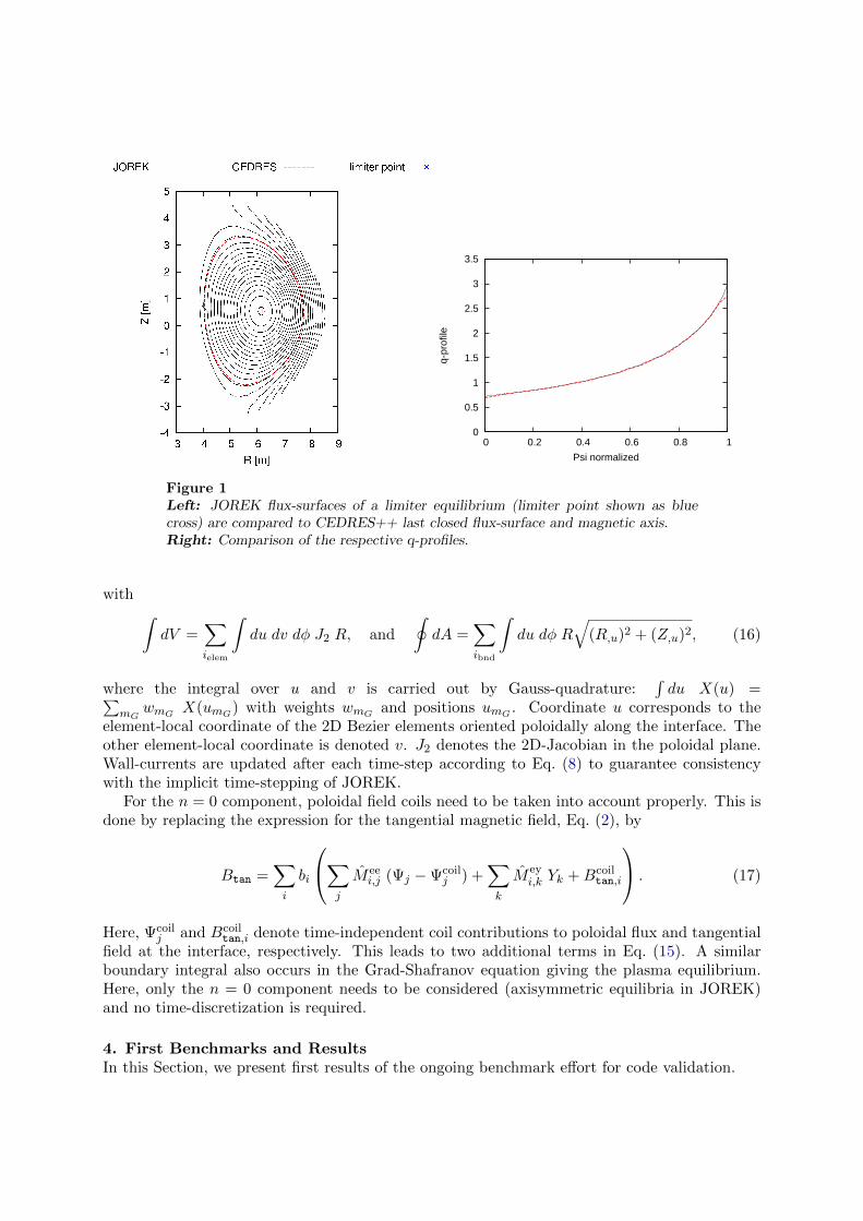
Figure 1Left: JOREK flux-surfaces of a limiter equilibrium (limiter point shown as bluecross) are compared to CEDRES++ last closed flux-surface and magnetic axis.Right: Comparison of the respective q-profiles.

with ∫dV =

∑ielem

∫du dv dφ J2 R, and

∮dA =

∑ibnd

∫du dφ R

√(R,u)2 + (Z,u)2, (16)

where the integral over u and v is carried out by Gauss-quadrature:∫du X(u) =∑

mGwmG X(umG) with weights wmG and positions umG . Coordinate u corresponds to the

element-local coordinate of the 2D Bezier elements oriented poloidally along the interface. Theother element-local coordinate is denoted v. J2 denotes the 2D-Jacobian in the poloidal plane.Wall-currents are updated after each time-step according to Eq. (8) to guarantee consistencywith the implicit time-stepping of JOREK.

For the n = 0 component, poloidal field coils need to be taken into account properly. This isdone by replacing the expression for the tangential magnetic field, Eq. (2), by

Btan =∑i

bi

∑j

M eei,j (Ψj −Ψcoil

j ) +∑k

M eyi,k Yk +Bcoil

tan,i

. (17)

Here, Ψcoilj and Bcoil

tan,i denote time-independent coil contributions to poloidal flux and tangentialfield at the interface, respectively. This leads to two additional terms in Eq. (15). A similarboundary integral also occurs in the Grad-Shafranov equation giving the plasma equilibrium.Here, only the n = 0 component needs to be considered (axisymmetric equilibria in JOREK)and no time-discretization is required.

4. First Benchmarks and ResultsIn this Section, we present first results of the ongoing benchmark effort for code validation.

0.01 0.1 1rwall [m] - 1

102

103

gro

wth

rat

e [s

-1]

CASTORCASTOR + STARWALL_CJOREK + STARWALL_J

ηJorek=1.e-5

ηJorek=1.e-6

ηJorek=1.e-7

Figure 2Left: Linear growth-rates of a tearing-mode in a circular plasma with concentricideal wall are compared between CASTOR using its own vacuum field module,CASTOR coupled with STARWALL, and JOREK coupled with STARWALL. Verygood agreement is observed for a variety of different plasma resistivities and plasma-wall distances.Right: The current potential distribution (arbitrary units) reflecting the 2/1 tearingmode structure is plotted during the linear phase (ηJorek = 1 · 10−6, rw = 1.2).

4.1. Free-boundary equilibriumComputing a free-boundary equilibrium with JOREK and comparing it to the results ofanother equilibrium solver allows to check some parts specific for n = 0 like poloidal field-coil contributions (see Sec. 3.2). We are considering an ITER-like limiter plasma. As seenfrom Figure 1, flux surfaces and q-profile of the JOREK equilibrium agree very well with theequilibrium computed by the CEDRES++ code [9]. Slightly different discretizations of thepoloidal field coils might be responsible for small remaining differences.

4.2. Tearing ModeA 2/1 tearing mode in a circular plasma with major radius R = 10, minor radius a = 1 anduniform plasma resistivity surrounded by an ideally conducting wall is considered. Figure 2shows excellent agreement between JOREK and the linear CASTOR code [10]. Repeatingthe simulation for a resistive wall with zero resistivity is physically identical, of course, butnumerically treated in a different way. The exact agreement we get here proves consistency.

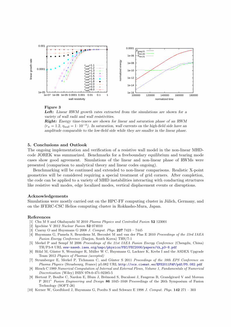
4.3. Resistive Wall ModeIn this Section, results for 2/1 resistive wall modes (RWMs) in a circular plasma with minorradius a = 1 and major radius R = 10 surrounded by a resistive wall are presented. The leftpart of Figure 3 shows linear growth rates obtained for different wall radii rw as a function of thewall resistivity. Clearly, the modes cannot be stabilized beyond a certain wall distance from theplasma even at very low wall resistivities. The right part of the Figure shows energy time-tracesduring the linear and saturation phase of a typical simulation.

1e-05

0.0001

0.001

1e-07 1e-06 1e-05 0.0001 0.001 0.01 0.1 1

linea

r gr

owth

rat

e

wall resistivity

rwall=1.1rwall=1.2rwall=1.3rwall=1.4rwall=1.5rwall=1.6rwall=1.8rwall=2.0rwall=4.0rwall=8.0

1e-16

1e-14

1e-12

1e-10

1e-08

1e-06

0.0001

100000 120000 140000 160000 180000

norm

aliz

ed e

nerg

y

normalized time

Emag,01Ekin,00Ekin,01

Figure 3Left: Linear RWM growth rates extracted from the simulations are shown for avariety of wall radii and wall resistivities.Right: Energy time-traces are shown for linear and saturation phase of an RWM(rw = 1.2, ηwall = 1 · 10−4). In saturation, wall currents on the high-field side have anamplitude comparable to the low-field side while they are smaller in the linear phase.

5. Conclusions and OutlookThe ongoing implementation and verification of a resistive wall model in the non-linear MHD-code JOREK was summarized. Benchmarks for a freeboundary equilibrium and tearing modecases show good agreement. Simulations of the linear and non-linear phase of RWMs werepresented (comparison to analytical theory and linear codes ongoing).

Benchmarking will be continued and extended to non-linear comparisons. Realistic X-pointgeometries will be considered requiring a special treatment of grid corners. After completion,the code can be applied to a variety of MHD instabilities interacting with conducting structureslike resistive wall modes, edge localized modes, vertical displacement events or disruptions.

AcknowledgementsSimulations were mostly carried out on the HPC-FF computing cluster in Julich, Germany, andon the IFERC-CSC Helios computing cluster in Rokkasho-Mura, Japan.

References[1] Chu M S and Okabayashi M 2010 Plasma Physics and Controlled Fusion 52 123001[2] Igochine V 2012 Nuclear Fusion 52 074010[3] Czarny O and Huysmans G 2008 J. Comput. Phys. 227 7423 – 7445[4] Huysmans G, Pamela S, Beurskens M, Becoulet M and van der Plas E 2010 Proceedings of the 23rd IAEA

Fusion Energy Conference (Daejon, South Korea) THS/7-1[5] Merkel P and Sempf M 2006 Proceedings of the 21st IAEA Fusion Energy Conference (Chengdu, China)

TH/P3-8 URL www-naweb.iaea.org/napc/physics/FEC/FEC2006/papers/th_p3-8.pdf

[6] Holzl M, Gunter S, Wenninger R, Muller W C, Huysmans G, Lackner K, Krebs I and the ASDEX UpgradeTeam 2012 Physics of Plasmas (accepted)

[7] Strumberger E, Merkel P, Tichmann C, and Gunter S 2011 Proceedings of the 38th EPS Conference onPlasma Physics (Strasbourg, France) p5.082 URL http://ocs.ciemat.es/EPS2011PAP/pdf/P5.082.pdf

[8] Hirsch C 1989 Numerical Computation of Internal and External Flows, Volume 1, Fundamentals of NumericalDiscretization (Wiley) ISBN 978-0-471-92385-5

[9] Hertout P, Boulbe C, Nardon E, Blum J, Bremond S, Bucalossi J, Faugeras B, Grandgirard V and MoreauP 2011” Fusion Engineering and Design 86 1045–1048 Proceedings of the 26th Symposium of FusionTechnology (SOFT-26)

[10] Kerner W, Goedbloed J, Huysmans G, Poedts S and Schwarz E 1998 J. Comput. Phys. 142 271 – 303

Appendix A. Relation between ideal and resistive response matricesBetween the ideal and resistive response-matrices, the relation

M idi,j ≡ M ee

i,j −∑k

M eyi,k M

yek,j (A.1)

must hold which becomes obvious when letting ηw → 0 and inserting Eq. (3) into Eq. (2). Also,the no-wall response can easily be identified as

Mnwi,j ≡ M ee

i,j (A.2)

when letting Yk → 0. Eqs. (A.1) and (A.2) can be used to cross-check some parts of theimplementation as both forms of the wall-treatment with eliminated wall-currents (Eq. (1)) andexplicitly treated wall-currents (Eqs. (2) and (3)) are implemented in JOREK.

Appendix B. Magnetic field tangential to the interfaceThe magnetic field in the JOREK reduced-MHD model is given by

B =F0

Reφ +

1

R∇Ψ× eφ. (B.1)

Its component tangential to the boundary of the JOREK computational domain (in the poloidalplane) can be determined from

Btan = (B× n) · eφ, (B.2)

where n denotes the unit normal vector of the interface and eφ the normalized toroidal basisvector. Inserting Eq. (B.1) and using vector identities, this can be written in the form

Btan = − 1

Reφ · [n× (∇Ψ× eφ)]

= − 1

Reφ ·

(n · eφ)︸ ︷︷ ︸≡0

∇Ψ− (n · ∇Ψ)eφ

=

1

Rn · ∇Ψ,

(B.3)

which can be identified in the boundary integral of Eq. (14) and replaced by the STARWALLresponse.