coupling dynamic models of climate and vegetation › refs › entclim › f › fo024.pdfclimate...

Global Change Biology (1998) 4, 561–579

Coupling dynamic models of climate and vegetation

J O N A T H A N A . F O L E Y, * S A M U E L L E V I S , * I . C O L I N P R E N T I C E 2 , † , D AV I D P O L L A R D ‡and S T A R L E Y L . T H O M P S O N §*Climate, People, and Environment Program (CPEP), Institute for Environmental Studies, University of Wisconsin, 1225 WestDayton Street, Madison, WI 53706, USA, †Global Systems Group, Department of Plant Ecology, The Ecology Building, LundUniversity, S-223 62 Lund, Sweden, ‡Earth System Science Center, Penn State University, University Park, PA 16802, USA,§Climate and Global Dynamics Division, National Center for Atmospheric Research (NCAR), PO Box 3000, Boulder, CO80307, USA

Abstract

Numerous studies have underscored the importance of terrestrial ecosystems as anintegral component of the Earth’s climate system. This realization has already led toefforts to link simple equilibrium vegetation models with Atmospheric General Circula-tion Models through iterative coupling procedures. While these linked models havepointed to several possible climate–vegetation feedback mechanisms, they have beenlimited by two shortcomings: (i) they only consider the equilibrium response ofvegetation to shifting climatic conditions and therefore cannot be used to exploretransient interactions between climate and vegetation; and (ii) the representations ofvegetation processes and land-atmosphere exchange processes are still treated by twoseparate models and, as a result, may contain physical or ecological inconsistencies.

Here we present, as a proof concept, a more tightly integrated framework for simulatingglobal climate and vegetation interactions. The prototype coupled model consists of theGENESIS (version 2) Atmospheric General Circulation Model and the IBIS (version 1)Dynamic Global Vegetation Model. The two models are directly coupled through acommon treatment of land surface and ecophysiological processes, which is used tocalculate the energy, water, carbon, and momentum fluxes between vegetation, soils,and the atmosphere. On one side of the interface, GENESIS simulates the physics andgeneral circulation of the atmosphere. On the other side, IBIS predicts transient changesin the vegetation structure through changes in the carbon balance and competitionamong plants within terrestrial ecosystems.

As an initial test of this modelling framework, we perform a 30 year simulation inwhich the coupled model is supplied with modern CO2 concentrations, observed oceantemperatures, and modern insolation. In this exploratory study, we run the GENESISatmospheric model at relatively coarse horizontal resolution (4.5° latitude by 7.5°longitude) and IBIS at moderate resolution (2° latitude by 2° longitude). We initializethe models with globally uniform climatic conditions and the modern distribution ofpotential vegetation cover. While the simulation does not fully reach equilibrium bythe end of the run, several general features of the coupled model behaviour emerge.We compare the results of the coupled model against the observed patterns of modernclimate. The model correctly simulates the basic zonal distribution of temperature andprecipitation, but several important regional biases remain. In particular, there is asignificant warm bias in the high northern latitudes, and cooler than observed conditionsover the Himalayas, central South America, and north-central Africa. In terms ofprecipitation, the model simulates drier than observed conditions in much of SouthAmerica, equatorial Africa and Indonesia, with wetter than observed conditions innorthern Africa and China.

Comparing the model results against observed patterns of vegetation cover showsthat the general placement of forests and grasslands is roughly captured by the model.In addition, the model simulates a roughly correct separation of evergreen and deciduousforests in the tropical, temperate and boreal zones. However, the general patterns of

© 1998 Blackwell Science Ltd. 561

562 J . A . F O L E Y et al.

global vegetation cover are only approximately correct: there are still significant regionalbiases in the simulation. In particular, forest cover is not simulated correctly in largeportions of central Canada and southern South America, and grasslands extend too farinto northern Africa.

These preliminary results demonstrate the feasibility of coupling climate models withfully dynamic representations of the terrestrial biosphere. Continued development offully coupled climate-vegetation models will facilitate the exploration of a broad rangeof global change issues, including the potential role of vegetation feedbacks within theclimate system, and the impact of climate variability and transient climate change onthe terrestrial biosphere.

Keywords: biosphere–atmosphere interactions, climate–vegetation feedback, coupled models

Introduction

The Earth’s physical climate system and biosphere coexistwithin a thin spherical shell, extending from the deepoceans to the upper atmosphere, that is driven by energyfrom the sun. The resulting interactions among the atmo-sphere, oceans, and terrestrial ecosystems give rise to thebiogeochemical, hydrological, and climate systems thatsupport life on this planet. During the last few centuries,both the terrestrial biosphere and physical climate systemhave been undergoing fundamental changes in responseto human activity. It is therefore of paramount importanceto improve our understanding of global-scale climaticand biospheric processes.

The Earth’s climate is, in part, controlled by the fluxesof energy, water, and momentum across the lower bound-ary of the atmosphere. Over the oceans, the exchange ofenergy and water with the atmosphere depends primarilyon the sea-surface temperature. Fluxes over land, on theother hand, are controlled by a more complex set ofattributes, including the state of the vegetation cover andsoils. Changes in vegetation, whether driven by climateor human activities, can substantially alter the physicalcharacteristics of the land surface, potentially leading tolarge feedbacks on the atmosphere. In fact, a numberof recent studies have suggested that feedbacks fromchanging global vegetation patterns may have played animportant role in determining climatic conditions duringthe recent geological past:d Possible role of vegetation feedbacks in initiating glaciations.Gallimore & Kutzbach (1996) and de Noblet et al. (1996)have indicated how changes in the position of the borealforest – tundra boundary (and the associated differencesin surface albedo between dark evergreen forests andsnow-covered tundra), may be partially responsible forinitiating ice age conditions during the Quaternary.According to this hypothesis, orbital variations and lowerCO2 concentrations initiate a trend towards glacial condi-

Correspondence: J.A. Foley, fax 11/608 262 5964

© 1998 Blackwell Science Ltd., Global Change Biology, 4, 561–579

tions, which is strongly amplified through the expansionof highly reflective tundra into the darker boreal forests.Previous climate modelling studies, which neglected thepotential for vegetation feedbacks, generally failed toproduce the conditions necessary to initiate past glaci-ations.d Boreal forest feedbacks on early Holocene warming. Inanother set of palaeoclimate sensitivity studies, Foleyet al. (1994) and TEMPO Authors (1996) discussed howa poleward shift in the boreal forest – tundra boundaryduring the early and middle Holocene epoch (roughly6000–9000 years before present) may have strongly ampli-fied orbitally induced warming of the high northernlatitudes. Once again, the vegetation feedback mechanismacts to amplify an initial shift in climate through changesin surface albedo associated with tundra and boreal forestecosystems. This vegetation feedback mechanism, whichmay strongly amplify high-latitude warming, should befurther examined in terms of future climate changescenarios.d A ‘green sahara’ and the African monsoon of the earlyHolocene. Finally, Kutzbach et al. (1996) and Claussen &Gayler (1997) have evaluated how the orbitally enhancedmonsoon rains of northern Africa may have been ampli-fied through vegetation feedbacks. The geological recordindicates that the Sahara of the early and middle Holocenewas a much wetter and more productive environmentthan present, with extensive grasslands, savannas andlakes (e.g. COHMAP Authors 1988). Such changes in theland surface (and the associated changes in albedo,leaf area, rooting depth, soil moisture, and evapo-transpiration) may have enhanced the strength of theAfrican monsoon. The same mechanism (but acting inreverse) was suggested by Charney et al. (1975) to explainincreasing droughts in the Sahel in terms of anthropo-genic desertification.

These palaeoclimate sensitivity studies, which havebeen partially corroborated by geological evidence, pro-

C O U P L I N G D Y N A M I C M O D E L S O F C L I M A T E A N D V E G E T A T I O N 563

vide a very powerful motivation to further examineclimate and vegetation interactions. In particular, futureglobal change scenarios must be re-evaluated to considerthe potential for vegetation feedback mechanisms. Forexample, scenarios of CO2-induced global warming,already amplified in the high latitudes by snow and sea-ice feedbacks, may be substantially modified by long-term changes in the boreal forest and tundra boundaries.Furthermore, several AGCM simulations have indicatedthat continental interiors may become much drier inresponse to global warming conditions, but this resulthas not considered the potential feedbacks caused bychanges in vegetation cover. In addition, it is hypothes-ized that the physiological effects of increasing atmo-spheric CO2 concentrations could significantly influenceterrestrial vegetation by decreasing stomatal conductanceand increasing canopy leaf area (Field et al. 1995), whichmay also give rise to significant feedbacks on the atmo-sphere (Pollard & Thompson 1995; Friend & Cox 1995;Henderson-Sellers et al. 1995; Sellers et al. 1996; Betts et al.1997). Clearly, models used to simulate future climatemust be improved to consider changes in vegetationcover, and their consequent feedbacks on the atmosphere.

Linking climate and vegetation models

When considering the potential interactions betweenvegetation and the atmosphere, we may distinguishbetween: (i) the rapid biophysical processes of energy,water, carbon, and momentum exchange; and (ii) thelong–term interactions which arise from fundamentalchanges in the vegetation cover. For over a decade, manyAGCMs have used land surface parameterizations (e.g.BATS of Dickinson et al. 1986; SiB of Sellers et al. 1986)to represent the rapid biophysical exchanges of energy,momentum, and water between terrestrial ecosystemsand the atmosphere (Sellers et al. 1997). Until recentlythese land surface parameterizations have been operatedby fixing the geographical distribution of vegetation types(Fig. 1a). Typically, each land gridcell of the AGCM isassigned a single vegetation type (e.g. tropical rainforest,boreal forest, tundra, desert), which has an associated setof biophysical characteristics, including leaf area index,albedo, rooting depth, and roughness length. However,using fixed patterns of global vegetation within climatemodels severely limits their use in studies of globalenvironmental change.

During the last few years, a few preliminary attemptsat linking models of vegetation cover to AGCMs havebeen made. Henderson-Sellers (1993) pioneered this workby operating the CCM1-Oz AGCM in conjunction withthe Holdridge (1947) equilibrium vegetation scheme. Inthis study, the Holdridge scheme is applied annually toupdate the geographical distribution of vegetation types


within the climate model. More specifically, the twomodels are iteratively linked through an equilibriumasynchronous coupling procedure (Fig. 1b), where asingle year of the climate model simulation is used todrive changes in the equilibrium distribution of vegeta-tion types which, in turn, are fed back into the AGCMland surface package. In principle, this iterating cycle ofequilibrium climate and equilibrium vegetation simula-tions is repeated until the results of both models convergeto some final state. In this initial study, Henderson-Sellersfound that the coupled behaviour of the CCM1-Oz andHoldridge models was stable, with no particular trendsor instabilities in the climate-vegetation system. In addi-tion, she found only regional-scale differences in thesimulation of modern climate between simulations per-formed with and without interactive vegetation cover.

In another effort to link climate and equilibrium vegeta-tion models, Claussen (1994) performed several simula-tions with the ECHAM AGCM linked to the BIOMEequilibrium vegetation model of Prentice et al. (1992). LikeHenderson-Sellers, Claussen also employed an iterativeequilibrium asynchronous coupling procedure to link theclimate and equilibrium vegetation models. However,in Claussen’s study the BIOME model was driven bymultiyear averages of the climate simulation, rather thanthe single-year climate simulations used in Henderson-Sellers (1993). Claussen also investigated the sensitivityof the coupled climate-vegetation to the specification ofinitial conditions. In particular, he compared the resultsof two coupled simulations: one initialized with theobserved geographical distribution of vegetation types,and another initialized with tropical forests replaced withsubtropical deserts and subtropical deserts replaced withtropical forests. His results showed that the equilibriumclimate was affected by the initial vegetation conditionsto permit savannas to persist in the desert of south-western Sahara. These results suggest that the coupledclimate-vegetation system, like many other nonlinearsystems, may arrive at different equilibrium statesdepending on the choice of initial conditions.

A few other studies have applied asynchronouslylinked climate-vegetation models to issues of climatechange. For example, de Noblet et al. (1996) linked theBIOME equilibrium vegetation model to the LMD AGCMto examine how changes in the boreal forest and tundraboundary may have contributed to the initiation ofglaciations during the Quaternary. Claussen (1998),Claussen (1997), and Claussen & Gayler (1997) usedthe coupled ECHAM-BIOME model to investigate theinfluence of initial vegetation conditions on changes inthe African and Indian monsoon during the modern andmiddle Holocene eras. Finally, Betts et al. (1997) haveused coupled climate-vegetation models to investigate

564 J . A . F O L E Y et al.

Fig. 1 Methods of coupling climate andvegetation models.

the potential role of vegetation feedbacks on futureclimatic change.

These exploratory studies all underscore the impor-tance of incorporating representations of changing vegeta-tion cover within climate models. However, they leaveseveral important areas open for further model develop-ment. In particular, the current set of linked climate-vegetation models have two major limitations:(a) Most existing vegetation models simulate only theequilibrium response of vegetation cover to changes inclimate. Models, like BIOME and the Holdridge scheme,are unable to simulate transient changes in vegetationcover in response to shifting environmental conditions,such as changing climate and CO2 concentrations. There-fore, current vegetation models cannot address the time-


dependent nature of the atmosphere–biosphere responseto climate variability or future climatic change.(b) Vegetation models and AGCM land surface para-meterizations are not always physically consistent. Forexample, in the coupled ECHAM-BIOME model, thereare two independent treatments of the surface waterand energy balance: one for describing land–atmosphereexchange processes (in ECHAM) and another for estimat-ing the soil moisture requirements of plants (in BIOME).In ECHAM evapotranspiration is calculated on an 80minute timestep using a detailed aerodynamic fluxformulation, while BIOME calculates evapotranspirationonce a day using a modified Priestley–Taylor formulationlinked to a soil water balance model (Claussen, pers.comm.). An additional limitation of most equilibrium


vegetation models is that they do not explicitly considerstructural attributes of vegetation, like leaf area indexand vegetation height, which are often required by AGCMland surface parameterizations. Ideally, land surfacephysics, ecological processes, and vegetation structureshould be simulated within a single, physically consistentmodel (Foley 1995).

To address these issues, a new group of fully dynamicbiosphere models has recently emerged. These state-of-the-art models, often called Dynamic Global VegetationModels (DGVMs), are designed to provide a more integ-rated and physically consistent simulation of land surfacephysics, ecological processes, and vegetation structure.Most importantly, DGVMs are also capable of simulatingtransient changes in ecosystem processes and vegetationstructure (Steffen et al. 1992; Walker 1994). Some DGVMs,including the Integrated Biosphere Simulator (IBIS) ofFoley et al. (1996), are also designed to be incorporateddirectly within AGCMs, thus providing a more completelinkage between atmospheric and ecological processes(Fig. 1c). IBIS has already been used off-line of an AGCMto investigate global patterns of water balance, primaryproductivity, and vegetation dynamics (Foley et al. 1996),and the potential impact of increasing CO2 concentrationson the hydrology of the Amazon basin (Costa & Foley,1997). Here we present a new modelling framework forsimulating atmosphere–biosphere interactions. Specific-ally, we have directly coupled the GENESIS global climatemodel to the IBIS dynamic global vegetation model.

IBIS — a dynamic global vegetation model forclimate studies

IBIS (version 1) is designed around a hierarchical model-ling framework (Fig. 2), in which information flowsbetween various subsystems at appropriate frequencies.IBIS represents a number of land surface and ecosystemphenomena, including:d land surface and physiological processes, including photo-synthesis, respiration, and stomatal behaviour, as well asthe surface energy, water, and momentum balanced phenological behaviour of leaf display and plant activityin response to changing climatic conditionsd transient changes in carbon balance and vegetation structureresulting from changes in primary productivity, competi-tion, carbon allocation, carbon turnover, and mortality

Land surface processes and phenology

IBIS includes a land surface module which simulates theenergy, water, carbon, and momentum balance of the soil–vegetation–atmosphere interface. This module borrowsmost of its basic structure from LSX (Pollard & Thompson1995; Thompson & Pollard 1995a,b), which is the original


land-surface parameterization scheme of the GENESISclimate model. Here the land-surface module operateson a relatively short timestep (30 min), which is also thetimestep used by the AGCM to simulate atmosphericdynamics. The module represents two vegetation layers(i.e. ‘woody plants’ and ‘herbaceous plants’) and six soillayers to simulate soil temperature, soil water, and soilice content over a total depth of 4.25 m. Physical processesin the vertical soil column include heat diffusion, liquidwater transport, uptake of liquid water by roots fortranspiration, and the freezing and thawing of soil ice.

Physiologically based formulations of C3 and C4 photo-synthesis (Farquhar et al. 1980; Collatz et al. 1991, 1992),stomatal conductance (Leuning 1995) and respiration(Amthor 1984) are used to simulate canopy gas exchangeprocesses. This approach provides a mechanistic linkbetween the exchange of water and CO2 between vegeta-tion canopies and the atmosphere (Collatz et al. 1991;Sellers et al. 1992; Amthor 1994; Bonan 1995). Because ofthe nonlinear response of physiological parameters tovarying environmental conditions, leaf-level processesare scaled to the canopy by assuming that the verticalprofile of Rubisco capacity is nearly optimized withrespect to net canopy photosynthesis (Field 1983; Sellerset al. 1992; Haxeltine & Prentice 1997).

Currently, IBIS uses very simple temperature and pro-ductivity criteria to control leaf display in winter-decidu-ous and drought-deciduous trees. While these algorithmsreflect some basic control of climate on phenology, theycould be improved to consider more processes, includingthe relationships between growing degree day require-ments for budburst and chilling period length (e.g. Mur-ray et al. 1989).

Vegetation structure

While previous vegetation models have focused on equi-librium vegetation patterns (e.g. Holdridge 1947; Prenticeet al. 1992; Neilson & Marks 1994; Haxeltine & Prentice1996), recent efforts have produced more highly general-ized approaches to simulating vegetation dynamics in awide range of environmental conditions. For global-scaleapplications, IBIS uses a simplified representation ofvegetation dynamics where plant growth and competitionare characterized by the ability of plants to capture lightand water from common resource pools. For example,tall woody plants (trees and shrubs) intercept light first,and therefore shade herbaceous plants. However, herb-aceous plants are able to preferentially capture soil mois-ture as it infiltrates through the soil. In this way, the modelcan simulate some of the basic features of competitionbetween trees and herbaceous plants. Furthermore, com-petition among woody plants and among herbaceousplants is driven by differences in the annual carbon

566 J . A . F O L E Y et al.

Fig. 2 Overview of the IBIS dynamic global vegetation model. IBIS represents a number of ecosystem processes occurring at differenttimescales. Land surface physics and canopy physiological processes are simulated on a short timestep (30 min), while vegetationphenology and vegetation dynamics are simulated on longer timesteps (1 day and 1 year, respectively).

balance resulting from differences in allocation, pheno-logy, leaf form, and photosynthetic pathway. Unlike mostother ecosystem models, IBIS explicitly simulates lightand water availability as part of the physics of the landsurface package during each 30 minute timestep.

In IBIS the vegetation cover is represented as a combina-tion of nine plant functional types (7 trees and 2 herb-aceous plants) that are adapted from Prentice et al. (1992).Plant functional types are defined to resolve a fewimportant features: basic physiognomy (e.g. trees andgrasses), leaf habit (e.g. evergreen and deciduous), photo-synthetic pathway (C3 and C4), and leaf form (broad-leaf and needle-leaf) (Woodward & Cramer 1996). Inorder to determine which plant functional types maypotentially exist within each gridcell, the model uses aset of simple climatic constraints (i.e. winter temperaturelimits, growing degree days, and minimum chillingrequirements). In off-line simulations, IBIS uses long-term climatic means to determine the limits of each plantfunctional type. However, when coupled to an AGCM,IBIS uses a 5-year running mean of the monthly averageclimatic parameters.

While IBIS-1 correctly simulates the basic global-scalepatterns of ecosystem processes and vegetation cover(Foley et al. 1996), the current version of the model hasseveral limitations, including a lack of explicit disturbancemechanisms (e.g. fire and windthrow). This omission has


important consequences on the ability of the model todescribe savannas and mixed forests, whose compositionis strongly affected by disturbance frequency. We alsoexpect that the representation of vegetation dynamicscould be improved by including parameterizations ofother subgrid and landscape-scale processes (Walker1994).

GENESIS — a global climate model

The global climate model used here is version 2 of theGENESIS (Global ENvironmental and Ecological Simula-tion of Interactive Systems) AGCM, which was developedat the National Center for Atmospheric Research (NCAR)for the main purposes of performing greenhouse andpalaeoclimatic experiments. An earlier version of themodel (version 1.02) has been described in Thompson &Pollard (1995a,b) and Pollard & Thompson (1994, 1995).The primary improvements to the model physics inversion 2 are documented in Thompson & Pollard (1997),along with a discussion of the model’s present-day climateand polar ice-sheet mass balance. In addition, a fewpalaeoclimatic applications of version 2 are described inPollard & Thompson (1997a,b). For brevity, only the mostsalient features of the model are outlined below.

The atmospheric component of GENESIS is a 3Dspectral general circulation model, which is nominally


operated at T31 spectral horizontal resolution (µ 3.75°latitude by 3.75° longitude), with 18 vertical levels, andan overall timestep of 30 min. In this exploratory study,we use a coarser configuration of R15 spectral resolution(µ 4.5° latitude by 7.5° longitude) to save on computingexpenses. We expect the GENESIS model’s simulation ofmodern-day climate to degrade as the resolution becomescoarser. Yet, for the purposes of illustrating the generalbehaviour of a coupled climate–vegetation model, thisresolution should be sufficient.

Solar radiation is modelled using a delta-Eddingtontwo-stream approximation for clear and cloudy fractionsof each atmospheric layer, with cloud overlap assumedto be random between layers. The radiation code of themodel treats the separate effects of greenhouse tracegases (CO2, CH4, N2O, CFC11, and CFC12) explicitly,assuming globally uniform mixing ratios (Wang et al.1991). O3 is prescribed from 3D monthly average climato-logical fields (Wang et al. 1995). The radiative effectsof tropospheric aerosols are also included, assuming auniform aerosol column over all nonice land points, witha prescribed exponential decrease with height.

GENESIS uses prognostic 3D cloud water amounts toseparately predict stratus, convective, and anvil cirrusclouds (Senior & Mitchell 1993; Smith 1990). A semi-Lagrangian algorithm is employed to transport water,while convective plumes and background diffusion mixwater vertically. The model includes the processes ofevaporation, conversion to precipitation, cloud dropletaggregation, and turbulent deposition of lowest-layercloud particles onto the surface. The model physics alsoaccounts for both ice and liquid cloud particles, butneglects the latent heat of freezing.

While the atmospheric portion of GENESIS operatesat coarse (R15) to moderate (T31) resolutions, land andocean surfaces are represented at a much finer spatialresolution of 2° latitude by 2° longitude. For each landgridcell, the topography and fraction of surface waterare derived from the high-resolution U.S. Navy FNOCglobal elevation dataset (Cuming & Hawkins 1981; Kine-man 1985). While GENESIS has been previously coupledto a variety of ocean models, in this study we prescribemonthly mean ocean temperatures from climatologicaldata (Shea et al. 1992).

Results of the coupled simulation

In this simulation, the coupled GENESIS–IBIS model isrun 30 years and is initialized with globally uniform airtemperatures (15 °C), soil temperatures (15 °C), and soilmoisture (50% of available pore space). The model’svegetation cover is initialized from a modified version ofHaxeltine & Prentice’s (1996) potential vegetation map.In particular, the Haxeltine & Prentice (1996) map is


simplified to represent only 7 vegetation types, insteadof the original 18 (Table 1). For each vegetation type, aset of leaf area index and biomass parameters are assignedfollowing Table 1. To avoid artifacts of the initial vegeta-tion map (e.g. unrealistically sharp boundaries betweenvegetation types), the resultant distributions of LAI andbiomass are smoothed through a 3-cell by 3-cell spatialaveraging filter.

During the first 10 years of the coupled model simula-tion, the model maintains the initial characteristics of thevegetation cover, so that the atmospheric circulation willbe allowed to equilibrate without interactive vegetation.Starting in Year 11, the coupled model allows the vegeta-tion cover to change, directly responding to the simulatedclimate. Simultaneously, a 5-year running-mean ofmonthly temperatures and growing degree days is usedto broadly bound the distribution of plant types. Clearlythis way of applying climatic limits on the geographicaldistribution of plant types is not process-based, but ratheris a very rough approximation for how plant distributionsrespond to shifting climatic patterns. We plan to replacethis with a more mechanistic formulation in a futureversion of the model, when we have explicit representa-tions of these processes.

In this exercise we have not employed a ‘flux correction’procedure, which is very common in atmosphere–oceanmodelling (e.g. Meehl 1990). In most coupled atmo-sphere–ocean models, key variables at the atmosphere–ocean interface (i.e. sea surface temperature and salinity)are restored towards observed climatological values, soas to keep the coupled model from ‘drifting’ into a poorrepresentation of the current climate. The main drawbackof this procedure is that it lacks a physical basis. Further-more, it is unclear how one would restore a coupledatmosphere–biosphere model towards observations,because the system interface cannot easily be character-ized by only a few well-observed parameters. As a result,we have decided not to use a flux correction techniqueto correct for biases in the AGCM and DGVM simulations.Thus we retain the physical consistency which this coup-ling scheme achieves. As coupled climate–vegetationmodels become more commonly used, this issue mayneed to be re-examined.

Simulated climate

According to Thompson & Pollard (1997), the present-dayclimate in GENESIS version 2 is significantly improved inmany regions compared to the earlier results for version1.02. Most of the improvements apparently stem fromthe greater horizontal and vertical resolutions, the newprognostic cloud scheme, and adjustments to the convect-ive plume scheme. In particular, precipitation, high-latitude surface temperatures, and snow and sea-ice

568 J . A . F O L E Y et al.

Table 1 Initial vegetation types. The types of vegetation defined in the potential modern vegetation map used as initialization for thissimulation. These vegetation types directly correspond to the types used by Haxeltine & Prentice (1996). Each vegetation type isassigned an upper canopy and a lower canopy initial LAI. In every continental gridcell, this LAI is partitioned among the IBIS plantfunctional types (pfts) permitted to exist according to simple climatic requirements (Foley et al. 1996). The resultant LAI maps forindividual pfts are smoothed through a 3 by 3 low pass filter and converted into leaf carbon using specific leaf area values for eachpft. Initial root carbon is assumed to equal initial leaf carbon. Initial wood carbon is such that in forests it adds up to 10 kg-C m–2

Woody Herb. IBIS herbaceousTree biomass IBIS tree pfts Herb. biomass pfts(grasses)

Simplified H & P H & P types LAI (kg-C m–2) (%) LAI (kg-C m–2) (%)

1 EVERGREEN FOREST 2, 4, 6, 7, 8 6.0 10.0 75% evergreen 1.0 0.10 50% warm25% deciduous 50% cool

2 DECIDUOUS FOREST 1, 5, 9 6.0 10.0 25% evergreen 1.0 0.10 50% warm75% deciduous 50% cool

3 MIXED FOREST 3 6.0 10.0 50% evergreen 1.0 0.10 50% warm50% deciduous 50% cool

4 SAVANNA GRASSLAND 10, 11, 12, 13 0.5 0.8 50% evergreen 4.0 0.40 75% warm50% deciduous 25% cool

5 XERIC VEGETATION 14, 15 0.8 1.3 50% evergreen 0.2 0.02 50% warm50% deciduous 50% cool

6 TUNDRA 17 0.0 0.0 none 2.0 0.20 100% cool7 DESERT 16, 18 0.0 0.0 none 0.0 0.00 none

distributions are all more realistic. However, Thompson& Pollard (1997) operated GENESIS at T31 horizontalresolution, while we use the more economical R15 reso-lution. As a result, we expect to have a somewhat poorersimulation of the modern climate. To compare the climateof the coupled model to observations, we average theresults over the last five years (Years 26–30) of thesimulation.

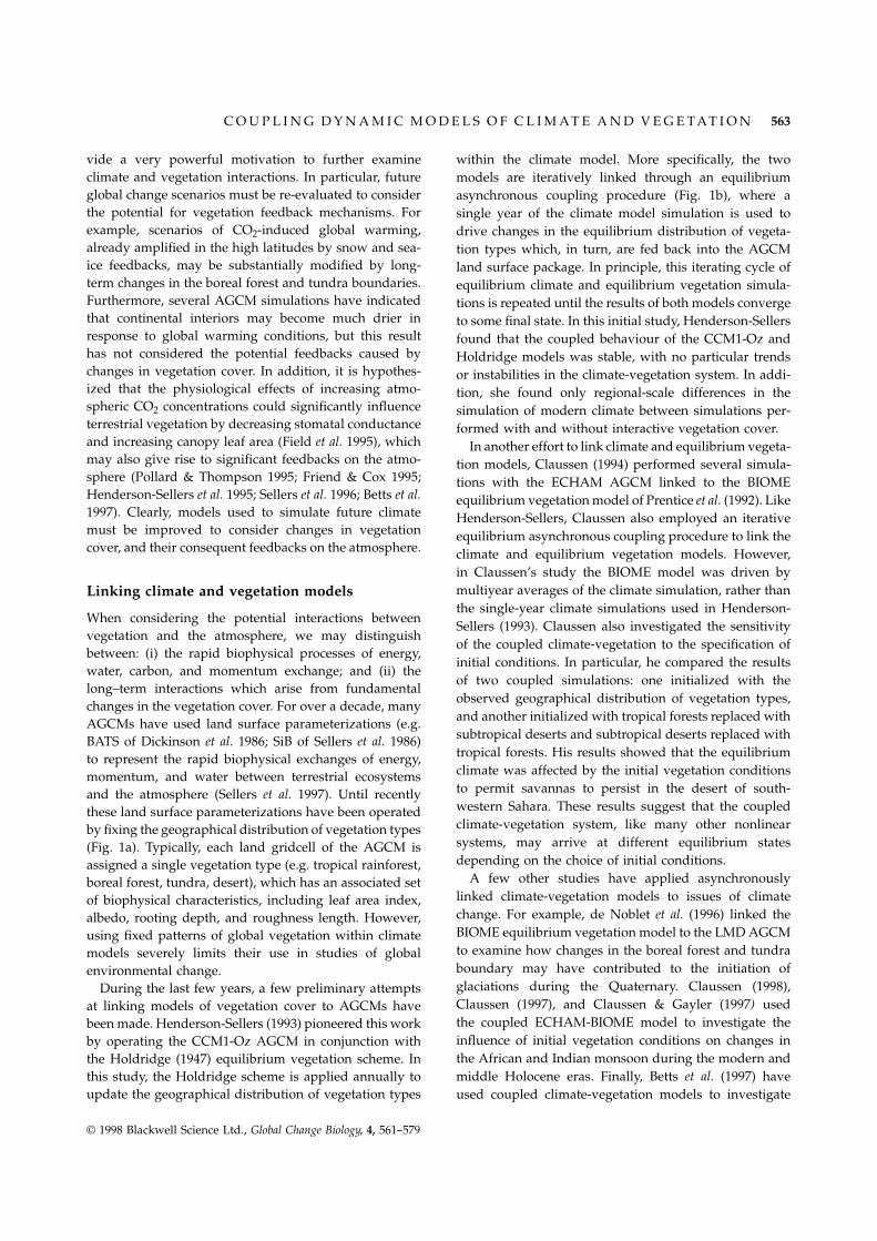
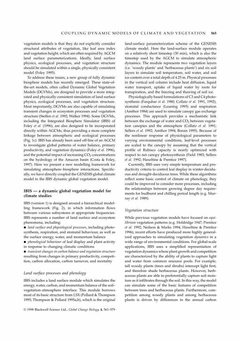
The general distribution of surface air temperatures(Fig. 3) appears to be well captured by the model;however, a significant warm bias is noticeable in the highnorthern latitudes. Comparing the simulated surface airtemperatures with observations of Legates & Willmott(1990, 1992) (Fig. 4), we see some significant regional-scale biases in the simulation. For example, there is alarge cold bias in the northern hemisphere over theHimalayan plateau and China, which we attribute toerroneous wintertime dynamical effects of the Himalayanplateau. Large areas of the northern continental interiorsare too warm, notably central Canada, Eastern Europe,and central Asia, which may have serious effects on thelocal vegetation. Despite these regional climatic biases,the zonal-average temperature fields (not shown) com-pare very favourably to observations and the results ofother coarse-resolution GCMs.

The global-average precipitation rate in the simulationis 1095 mm y–1, which is within the range of observedclimatologies (e.g. 1153 mm y–1, Legates & Willmott 1992).Over land, annual-average precipitation is 865 mm y–1

(compared to 806 mm y–1 and 864 mm y–1 accordingto Baumgartner & Reichel (1975) and UNESCO (1978),


Fig. 3 Initial vegetation cover of the coupled model. We initializethe coupled climate–vegetation model (see Table 1) with theobserved distribution of potential vegetation types (adaptedfrom Haxeltine & Prentice 1996).

respectively), and annual evapotranspiration is simulatedto be µ 75% of the precipitation (compared to 65% and61%, according to Baumgartner & Reichel and UNESCO,respectively). While the zonal mean patterns of precipita-


Fig. 4 Simulated patterns of surface air temperature. The general distribution of surface air temperatures is well captured by themodel; however, a significant warm bias is noticeable in the high northern latitudes. Surface fields from the atmosphere are passed tothe surface grid (2° latitude by 2° longitude), where they are used in the surface physics and ecosystem dynamics calculations.

tion (not shown) agree well with observations, regionalscale differences between observed and simulated (Fig. 5)precipitation may be large (Fig. 6). There are a few areaswhose annual rainfall is much less than observed, mostnotably the Amazon Basin and southern South America,central Africa and Indonesia, which may have seriouseffects on the vegetation cover. The model also tends toslightly underestimate rainfall over northern continentalinteriors between µ 40° and 60° N. The model simulateswetter than observed conditions in northern Africa andChina. Work is in progress to improve these shortcomings;however, the general patterns of simulated precipitationare reasonably realistic for medium- to low-resolutionAGCMs, and may be adequate for the initial explorationof vegetation–climate feedback mechanisms.


Simulated net primary productivity and vegetationcover

While this is a relatively long (30 year) simulation bymost AGCM standards, it is important to note that thevegetation component of the coupled model has not fullyreached equilibrium. By the end of the simulation, globalnet primary productivity (NPP) has roughly stabilized(Fig. 8a), but leaf area index (LAI) (Fig. 8b) and biomass(Fig. 8c) have not, particularly in regions which haveexperienced a large change in vegetation cover duringthe simulation. We expect, based on forest LAI andbiomass data, as well as our experience with IBIS offline,that LAI will equilibrate after another decade or two,while biomass will equilibrate after a few more decades

570 J . A . F O L E Y et al.

Fig. 5 Simulated minus observed patterns of surface air temperature. Here we see regional-scale biases in the temperature simulationplotted only over land. GENESIS produces a large cold bias over the Himalayan plateau and China, while large areas of the northerncontinental interiors are too warm, notably central Canada, Eastern Europe, and central Asia. Observed temperatures are taken fromthe Legates & Willmott (1990, 1992) climate dataset.

in the tropics and will continue to change for a centuryor more in slower-growing forests of cold climates.

Net primary productivity is often used as an index tocompare ecosystem activity, and its relationship to cli-mate. The global patterns of NPP (Fig. 9a) simulated bythe coupled model are strongly driven by the modelledclimate: areas of high NPP are in warm and moistclimates, while the least productive areas include subtrop-ical deserts, mountain ranges, and polar regions. In thissimulation, global total NPP is 83 Gt-C y–1, which isfairly high compared to other model-based estimates (e.g.Foley 1994). This value would have declined in a longersimulation due to the accumulation of respiring woodybiomass.

The simulated vegetation cover may be represented bythe geographical distributions of leaf area index (LAI)and biomass. The global distribution of total LAI (Fig. 9b)


shows the relative density of vegetation cover, which isstrongly determined by the modelled climate: areas ofhighest LAI include the rainforests of South America,Africa, and Asia, and forests of North America and EastAsia. Total vegetation biomass (Fig. 9c) follows this samebasic pattern, with high biomass in tropical and temperateforests, and low biomass in deserts and high-latitudeareas.

While some very basic geographical patterns of globalvegetation cover appear to be qualitatively captured bythe coupled model, there are still many areas that arepoorly simulated. For example, the forest and grasslandcover is underestimated in a large section of SouthAmerica as a result of the drier than observed conditionssimulated by GENESIS. A similar bias in the climatemodel (i.e. warmer than observed temperatures, lowerthan observed precipitation) results in very low produc-


Fig. 6 Simulated Patterns of Precipitation.

tivity and forest cover south-west of Canada’s HudsonBay. Conversely, anomalously wet conditions permitgrasslands to penetrate parts of the southern Sahara andArabian deserts.

We may also compare the geographical distributionsof LAI for individual plant types, to demonstrate thatmany basic patterns of vegetation geography are simu-lated fairly well by the coupled model (Figs 10 and 11).The model retains a clear separation of forests, grasslands,and tundra, with grasslands and tundra dominatingthe semiarid and high-latitude regions of the world.Grasslands are scattered throughout central Asia, centralNorth America, central Australia, and the semiaridregions of Africa and South America. Because of the lackof natural disturbance mechanisms, particularly fire, themodel does not simulate the large areas of savannavegetation in Africa and South America.

In the forested portions of the world, the model clearly


indicates a separation of evergreen-dominated anddeciduous-dominated forests (Fig. 10a and b). Forexample, in the high-latitudes, the model successfullysustains a boreal deciduous (i.e. Larix dominated) forestin eastern Siberia, and evergreen-dominated foreststhroughout the rest of the circumpolar boreal zone. Themid-latitude forests of Europe, eastern North America,and east Asia are a mixture of evergreen and deciduoustrees, but deciduous trees clearly dominate the core ofthe temperate forest regions (eastern North America,western Europe, and portions of east Asia). In the tropics,the model includes regions of drought deciduous forestsin the areas of seasonal rainfall, and tropical evergreenforests in the core of annual rainfall in the Amazon basin,central Africa, and Indonesia. In south-central Africa,however, tropical deciduous trees are shown to give wayto lush grasslands, because of cooler than observedtemperatures in the region.

572 J . A . F O L E Y et al.

Fig. 7 Simulated minus observed patterns of precipitation. While the zonal patterns of precipitation agree well with observations (notshown), regional-scale differences between observed and simulated precipitation (plotted only over land) may be large. The modelsimulates drier than observed conditions in much of South America, equatorial Africa and Indonesia, with wetter than observedconditions in northern Africa and China. The model also tends to slightly underestimate rainfall over northern continental interiorsbetween µ 40° to 60° N. Observed precipitation rates are taken from the Legates & Willmott (1990, 1992) climate dataset.

Fig. 8 Simulated trends of (a) Net Primary Production (NPP), (b) Average Leaf Area Index (LAI), and (c) average biomass. The trendin the global total NPP (a) appears to roughly stabilize by the end of the simulation, while the trends in the LAI (b) and especiallythe biomass (c) do not.



Fig. 9 Simulated patterns of (a) Net Primary Production (NPP),(b) Total Leaf Area Index (LAI), and (c) total biomass. Theresulting patterns of NPP (a) in the coupled model (averagedbetween years 26 and 30) are strongly driven by the simulatedclimate: areas of high NPP are in warm and moist climates,while the least productive areas include subtropical deserts,mountain ranges, and polar regions. The same applies to totalLAI (b) and total biomass (c).

Vegetation feedbacks on climate

To assess the potential feedbacks the interactive vegeta-tion cover may have on the climate, we compare twoperiods of simulation: one with fixed vegetation (Years6–10), and one with interactive vegetation (Years 26–30).

The interactive changes in vegetation cover result insignificant (at the 95% confidence level) temperaturechanges in several regions (Fig. 12). For example, thechanging vegetation cover causes cooling over thesouthern Sahara and Arabian deserts, mainly during thedrier seasons (boreal autumn, winter, and spring), whichcan be attributed to the northward expansion of grass-lands. In the early stages of the simulation, the modelplaces a stronger than observed monsoon over northern


Africa, permitting grasslands to penetrate northward. Theensuing changes in vegetation result in greater evapo-transpiration, which in part explains lower temperaturesduring the drier times of year. Furthermore, greateramounts of atmospheric moisture may cause additionalcloudiness, less solar radiation at the surface, and coolertemperatures. Conversely, a reduction in vegetation covercauses significant warming over south-central Africa inaustral summer, over much of south-eastern SouthAmerica in austral summer, and in central Asia duringboreal summer. Differences in relative humidity (notshown) also show a clear signal of the effects of interactivevegetation, with moister conditions over much of theSahara and Arabian deserts, and drier conditions incentral Asia.

574 J . A . F O L E Y et al.

Fig. 10 Simulated Leaf Area Index for (a) Evergreen Trees, (b)Deciduous Trees, and (c) Herbaceous Plants. The resultingpatterns of LAI at the end of the simulation (averaged betweenYears 26 and 30) result from the interactions between the climateand vegetation cover. These results show that the generalplacement of forests and grasslands is roughly captured by thecoupled model. The model also simulates a roughly correctseparation of evergreen and deciduous forests in the tropical,temperate, and boreal zones. However, the general patterns ofglobal vegetation cover are only approximately correct: thereare still significant regional biases in the simulation. In particular,forest cover is not simulated correctly in large portions of centralCanada and southern South America, and grasslands extend toofar into northern Africa.

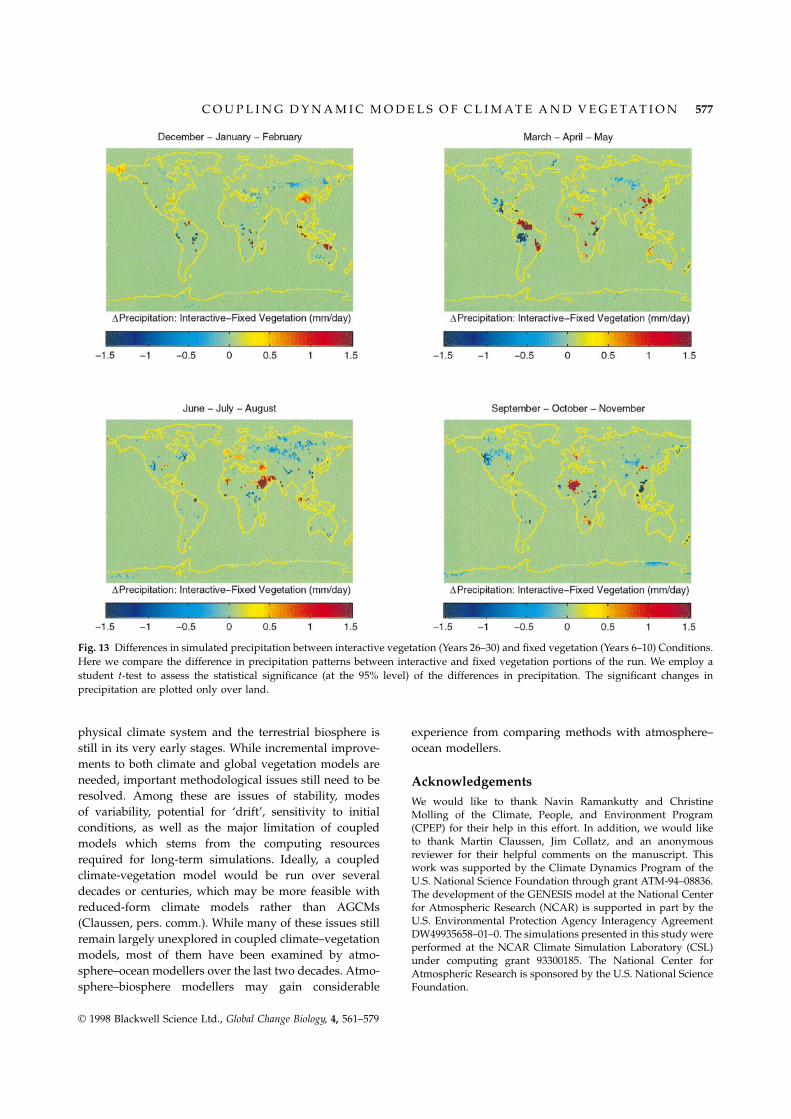
Changes in precipitation resulting from the interactivevegetation cover are not as clear at the 95% confidencelevel (Fig. 13). Most notably, we observe an increase inprecipitation over part of the Sahara late in the wetseason (boreal autumn) and the southern Arabian desertduring the wettest season (boreal summer). The effectsof interactive vegetation cover also cause significantincreases in snow cover at the southern edge of the borealforest and significant decreases in regions dominatedby tundra (not shown). It is important to note thatprecipitation displays greater interannual variability thantemperature and relative humidity, making it difficult fora t-test to capture the significance of the changes resultingfrom interactive vegetation.


Overall, the differences in climate resulting from inter-active changes in vegetation cover are relatively smallcompared to the intrinsic biases of the AGCM. The largestchanges in climate are associated with changes in theposition of desert/grassland and forest/tundra ecotones,which have already been implicated as centres of actionin previous climate–vegetation modelling studies (e.g.Claussen 1994; Foley et al. 1994).

Conclusions

Scenarios of future climate change must be re-evaluatedto consider the potential for vegetation feedbackmechanisms. In particular, the effects of several hypo-


Fig. 11. Simulated Leaf Area Index for each plant functional type.

thesized vegetation feedback mechanisms should beinvestigated, including: (a) changes in albedo resultingfrom shifting boreal forest and tundra boundaries, (b)changes in the extent of deserts and the resulting


changes in albedo and evapotranspiration, (c) increasesin mid-continental aridity, with the consequent changesin vegetation cover and soil moisture, and (d) changesin vegetation cover and evapotranspiration directly

576 J . A . F O L E Y et al.

Fig. 12 Differences in simulated temperature between interactive vegetation (Years 26–30) and Fixed Vegetation (Years 6–10) Conditions.To assess how the interactive vegetation cover may affect the overall climate of the model, we compare the surface air temperaturepatterns between interactive vegetation (Years 26–30) and fixed vegetation (Years 6–10) portions of the run. We employ a student t-test to assess the statistical significance (at the 95% level) of the differences in temperature. The significant changes in temperature areplotted only over land.

resulting from the physiological effects of increasedCO2 concentrations. Using coupled climate–vegetationmodels could help elucidate the role of vegetationfeedback mechanisms on future climate.

Previous studies, including Henderson-Sellers (1993)and Claussen (1994), have demonstrated the feasibilityof linking simple equilibrium vegetation models withatmospheric general circulation models. While theseexploratory efforts have highlighted the importance ofrepresenting vegetation cover within AGCMs, theyhave suffered from two limitations: (a) the equilibriumnature of current vegetation models, and (b) possibleinconsistencies between vegetation models and landsurface parameterizations. Ideally, AGCMs should bedirectly coupled to fully dynamic and integrated modelsof the biosphere, where land surface physics, ecological


processes, and vegetation dynamics would be simulatedwithin a single, physically consistent framework (Foley1995). Here we have taken the next logical step ofcoupling an AGCM with a fully dynamic and integratedglobal vegetation model.

In any coupled modelling exercise, it is important toexamine the variability of the system across a widevariety of timescales. Unfortunately, this initial simula-tion is not long enough for us to judge whether theclimate–vegetation system will remain stable aroundthe simulated mean conditions or it will oscillate witha discernible long-term trend. Longer simulations wouldalso be required to see if the coupled model exhibitsa ‘climate drift’, equivalent to what has been seen inmany coupled atmosphere–ocean models.

Modelling the dynamical interactions between the


Fig. 13 Differences in simulated precipitation between interactive vegetation (Years 26–30) and fixed vegetation (Years 6–10) Conditions.Here we compare the difference in precipitation patterns between interactive and fixed vegetation portions of the run. We employ astudent t-test to assess the statistical significance (at the 95% level) of the differences in precipitation. The significant changes inprecipitation are plotted only over land.

physical climate system and the terrestrial biosphere isstill in its very early stages. While incremental improve-ments to both climate and global vegetation models areneeded, important methodological issues still need to beresolved. Among these are issues of stability, modesof variability, potential for ‘drift’, sensitivity to initialconditions, as well as the major limitation of coupledmodels which stems from the computing resourcesrequired for long-term simulations. Ideally, a coupledclimate-vegetation model would be run over severaldecades or centuries, which may be more feasible withreduced-form climate models rather than AGCMs(Claussen, pers. comm.). While many of these issues stillremain largely unexplored in coupled climate–vegetationmodels, most of them have been examined by atmo-sphere–ocean modellers over the last two decades. Atmo-sphere–biosphere modellers may gain considerable


experience from comparing methods with atmosphere–ocean modellers.

AcknowledgementsWe would like to thank Navin Ramankutty and ChristineMolling of the Climate, People, and Environment Program(CPEP) for their help in this effort. In addition, we would liketo thank Martin Claussen, Jim Collatz, and an anonymousreviewer for their helpful comments on the manuscript. Thiswork was supported by the Climate Dynamics Program of theU.S. National Science Foundation through grant ATM-94–08836.The development of the GENESIS model at the National Centerfor Atmospheric Research (NCAR) is supported in part by theU.S. Environmental Protection Agency Interagency AgreementDW49935658–01–0. The simulations presented in this study wereperformed at the NCAR Climate Simulation Laboratory (CSL)under computing grant 93300185. The National Center forAtmospheric Research is sponsored by the U.S. National ScienceFoundation.

578 J . A . F O L E Y et al.

References

Amthor JS (1984) The role of maintenance respiration in plantgrowth. Plant, Cell and Environment, 7, 561–569.

Amthor JS (1994) Scaling CO2-photosynthesis relationships fromthe leaf to the canopy. Photosynthesis Research, 39, 321–350.

Baumgartner A, Reichel E (1975) The World Water Balance:Mean Annual Global Continental and Maritime Precipitation,Evaporation, and Runoff. Elsevier, New York, 179pp.

Betts RA, Cox PM, Lee SE, Woodward FI (1997) Contrastingphysiological and structural vegetation feedbacks in climatechange simulations. Nature, 387, 796–799.

Bonan GB (1995) Land-atmosphere CO2 exchange simulated bya land surface process model coupled to an atmosphericgeneral circulation model. Journal of Geophysical Research, 100,2817–2831.

Charney J, Stone PH, Quirk WJ (1975) Drought in the Sahara: Abiogeophysical mechanism. Science, 187, 434–435.

Claussen M (1994) Coupling global biome models with climatemodels. Climate Research, 4, 203–221.

Claussen M (1997) Modeling bio-geophysical feedback in theAfrican and Indian monsoon region. Climate Dynamics, 13,247–257.

Claussen M (1998) On multiple solutions of the atmosphere-vegetation system in present-day climate. Global ChangeBiology, this issue.

Claussen M, Gayler V (1997) The greening of Sahara during themid-Holocene: results of an interactive atmosphere–biomemodel. Global Ecology and Biogeography Letters, in press.

Cohmap (1988) Climatic changes of the last 18000 years:observations and model simulations. Science, 241, 1043–1052.

Collatz GJ, Ball JT.Grivet C, Berry JA (1991) Physiological andenvironmental regulation of stomatal conductance,photosynthesis and transpiration: a model that includes alaminar boundary layer. Agricultural And Forest Meteorology,54, 107–136.

Collatz GJ, Ribas-Carbo M, Berry JA (1992) Coupledphotosynthesis-stomatal conductance model for leaves of C4

plants. Australian Journal of Plant Physiology, 19, 519–538.Costa MH, Foley JA (1997) The water balance of the Amazon

basin dependence on vegetation cover and canopyconductance. Journal of Geophysical Research – Atmospheres,102, 23,973–23,989.

Cuming MJ, Hawkins BA (1981) TERDAT: The FNOC systemfor terrain data extraction and processing. Technical ReportM11 Project, M254 (2nd edn). Prepared for Fleet NumericalOceanography Center, Monterey: Meteorology InternationalInc.

Dickinson RE, Henderson-Sellers A, Kennedy PJ, Wilson MF(1986) Biosphere-Atmosphere Transfer Scheme (BATS) forthe NCAR CCM. NCAR Technical Note, NCAR/TN-275-STR, Boulder, CO, 69pp.

Farquhar GD, von Caemmerer S, Berry JA (1980) A biochemicalmodel of photosynthetic CO2 assimilation in leaves of C3

species. Planta, 149, 78–90.Field C (1983) Allocating leaf nitrogen for the maximization of

carbon gain: leaf age as a control on the allocation program.Oecologia, 56, 341–347.

Field CB, Jackson RB, Mooney HA (1995) Stomatal responses to


increased CO2 implications from the plant to the global scale.Plant, Cell And Environment, 18, 1214–1225.

Foley JA (1994) Net primary productivity in the terrestrialbiosphere: the application of a global model. Journal ofGeophysical Research, 99, 20773–20783.

Foley JA (1995) Numerical models of the terrestrial biosphere.Journal of Biogeography, 22, 837–842.

Foley JA, Kutzbach JE.Coe MT, Levis S (1994) Feedbacks betweenclimate and boreal forests during the Holocene epoch. Nature,371, 52–54.

Foley JA, Prentice CI.Ramankutty N.Levis S.Pollard D.Sitch S,Haxeltine A (1996) An integrated biosphere model of landsurface processes, terrestrial carbon balance, and vegetationdynamics. Global Biogeochemical Cycles, 10, 603–628.

Friend AD, Cox PM (1995) Modelling the effects of atmosphericCO2 on vegetation–atmosphere interactions. AgriculturalForest Meteorology, 73, 285–295.

Gallimore RG, Kutzbach JE (1996) Role of orbitally inducedchanges in tundra area in the onset of glaciation. Nature, 381,503–505.

Haxeltine A, Prentice IC (1996) BIOME3: An equilibriumterrestrial biosphere model based on ecophysiologicalconstraints, resource availability and competition amongplant functional types. Global Biogeochemical Cycles, 10, 693–709.

Haxeltine A, Prentice IC (1997) A general model for the lightuse efficiency of primary production. Functional Ecology, 10,551–561.

Henderson-Sellers A (1993) Continental vegetation as a dynamiccomponent of a global climate model: a preliminaryassessment. Climatic Change, 23, 337–377.

Henderson-Sellers A, Mcguffie K, Gross C (1995) Sensitivityof global climate model simulations to increased stomatalresistance and CO2 increases. Journal of Climate, 8, 1738–1756.

Holdridge LR (1947) Determination of world plant formationsfrom simple climatic data. Science, 105, 367–368.

Kineman J (1985) FNOC/NCAR global elevation, terrain, andsurface characteristics. Digital Dataset, 28 MB, Boulder:NOAA National Geophysical Data Center.

Kutzbach JE, Bonan G, Foley JA, Harrison SP (1996) Vegetationand soil feedbacks on the response of the African monsoonto orbital forcing in the early to middle Holocene. Nature,384, 623–626.

Legates DR, Willmott CJ (1990) Mean seasonal and spatialvariability in gauge-corrected, global precipitation. Int. J.Climatol., 111–127.

Legates DR, Willmott CJ (1992) A comparison of GCM simulatedand observed mean January and July precipitation.Paleogeography, Paleoclimatology, Paleoecology (Global andPlanetary Change Section), 97, 345–363.

Leuning R (1995) A critical appraisal of a combined stomatal-photosynthesis model for C3 plants. Plant, Cell andEnvironment, 18, 339–355.

Meehl GA (1990) Development of global coupled ocean-atmosphere general circulation models. Climate Dynamics, 5,19–33.

Murray MB, Cannell MGR, Smith I (1989) Date of budburst offifteen tree species in Britain following climatic warming.Journal of Applied Ecology, 26, 693–700.


Neilson RP, Marks D (1994) A global perspective of regionalvegetation and hydrologic sensitivities from climatic change.Journal of Vegetation Science, 5, 715–730.

de Noblet NI, Prentice IC, Joussaume S.Texier D.Botta A,Haxeltine A (1996) Possible role of atmosphere–biosphereinteractions in triggering the last glaciation. GeophysicalResearch Letters, 23, 3191–3194.

Pollard D, Thompson SL (1994) Sea-ice dynamics and CO2

sensitivity in a global climate model. Atmosphere-Ocean, 32,449–467.

Pollard D, Thompson SL (1995) Use of a land-surface-transferscheme (LSX) in a global climate model: the response todoubling stomatal resistance. Global and Planetary Change, 10,129–161.

Pollard D, Thompson SL (1997a) Climate and ice-sheet massbalance at the last glacial maximum from the GENESISversion 2 global climate model. Quaternary Science Reviews,in press.

Pollard D, Thompson SL (1997b) Driving a high-resolutiondynamic ice-sheet model with GCM climate: Ice-sheetinitiation at 116000 B.P. Annals of Glaciology, in press.

Prentice C, Cramer W, Harrison SP, Leemans R, Monserud RA,Solomon AM (1992) A global biome model based on plantphysiology and dominance, soil properties and climate.Journal of Biogeography, 19, 117–134.

Sellers PJ, Berry JA, Collatz GJ, Field CB, Hall FG (1992)Canopy reflectance, photosynthesis, and transpiration. III. Areanalysis using improved leaf models and a new canopyintegration scheme. Remote Sensing of the Environment, 42,187–216.

Sellers PJ, Bounoua L, Collatz GJ, Randall DA, Dazlich DA, LosSO, Berry JA, Fung I, Tucker CJ, Field CB, Jensen TG(1996) Comparison of radiative and physiological effects ofatmospheric CO2 on climate. Science, 271, 1402–1406.

Sellers PJ, Dickinson RE, Randall DA, Betts AK, Hall FG, BerryJA, Collatz GJ, Denning AS, Mooney HA, Nobre CA, SatoN, Field CB, Henderson-Sellers A (1997) Modeling theexchanges of energy, water, and carbon between continentsand the atmosphere. Science, 275, 502–509.

Sellers PJ, Mintz Y, Sud YC, Dalcher A (1986) A simple biosphere


model (SiB) for use within general circulation models. Journalof Atmospheric Science, 43, 505–531.

Senior CA, Mitchell JFB (1993) Carbon dioxide and climate:the impact of cloud parameterization. Journal of Climate, 6,393–418.

Shea DJ, Trenberth KE, Reynolds RW (1992) A Global MonthlySea Surface Temperature Climatology. Journal of Climate, 5,987–1001.

Smith RNB (1990) A scheme for predicting layer clouds andtheir water content in a general circulation model. QuarterlyJournal of the Royal Meteorological Society, 116, 435–460.

Steffen WL, Walker BH, Ingram JS, Koch GW (eds) (1992) Globalchanges and terrestrial ecosystems: The operational plan.Global Change Rep., 21, 95pp.. International Geosphere–Biosphere Programme, Stockholm.

Tempo (1996) Potential role of vegetation feedback in the climatesensitivity of high-latitude regions: A case study at 6000years B.P. Global Biogeochemical Cycles, 10, 727–736.

Thompson SL, Pollard D (1995a) A global climate model(GENESIS) with a land-surface transfer scheme (LSX). PartI: present climate simulation. Journal of Climate, 8, 732–761.

Thompson SL, Pollard D (1995b) A global climate model(GENESIS) with a land-surface transfer scheme (LSX). PartII: CO2 sensitivity. Journal of Climate, 8, 1104–1121.

Thompson SL, Pollard D (1997) Greenland Antarctic massbalances for present and doubled atmospheric CO2 from theGENESIS version 2 global climate model. Journal of Climate,10, 871–900.

Unesco (1978) World Water Balance and Water Resources of theEarth. Paris/Leningrad, 663pp.

Walker B (1994) Landscape to regional-scale responses ofterrestrial ecosystems to global change. Ambio, 23, 67–73.

Wang W-C, Liang X-Z.Dudek MP.Pollard D, Thompson SL (1995)Atmospheric ozone as a climate gas. Atmospheric Research,37, 247–256.

Wang W-C, Shi G-Y, Kiehl JT (1991) Incorporation of thermalradiative effect of CH4, N2O, CF2Cl2, and CFCl3 into theNCAR Community Climate Model. Journal of GeophysicalResearch, 96, 9097–9103.

Woodward FI, Cramer W (1996) Plant functional types andclimatic changes: Introduction. Journal of Vegetation Science,7, 306–308.

coupling dynamic models of climate and vegetation › refs › entclim › f › fo024.pdfclimate...

Documents