coupled fixed point theorems for generalized mizoguchi

RESEARCH Open Access

Coupled fixed point theorems for generalizedMizoguchi-Takahashi contractions withapplicationsLjubomir Ćirić1, Boško Damjanović2, Mohamed Jleli3 and Bessem Samet3*

* Correspondence: [email protected] of Mathematics, KingSaud University, Riyadh, SaudiArabiaFull list of author information isavailable at the end of the article

Abstract

We derive some new coupled fixed point theorems for nonlinear contractive mapsthat satisfied a generalized Mizoguchi-Takahashi’s condition in the setting of orderedmetric spaces. Presented theorems extends and generalize many well-known resultsin the literature. As an application, we give an existence and uniqueness theorem forthe solution to a two-point boundary value problem.2000 Mathematics Subject Classification: 54H25; 47H10.

Keywords: coupled fixed point, ordered metric space, mixed monotone mapping,generalized Mizoguchi-Takahashi’s contraction, two-point boundary value problem

1 IntroductionLet (X, d) be a metric space. Denote by P(X) the set of all nonempty subsets of X and

CB(X) the family of all nonempty closed and bounded subsets of X. A point x in X is a

fixed point of a multivalued map T : X ® P(X), if x Î Tx. Nadler [1] extended the

Banach contraction principle to multivalued mappings.

Theorem 1.1 (Nadler [1]) Let (X, d) be a complete metric space and let T : X ® CB

(X) be a multivalued map. Assume that there exists r Î [0,1) such that

H(Tx,Ty) ≤ rd(x, y)

for all x, y Î X, where H is the Hausdorff metric with respect to d. Then T has a fixed

point.

Reich [2] proved the following generalization of Nadler’s fixed point theorem.

Theorem 1.2 (Reich [2]) Let (X, d) be a complete metric space and T : X ® C(X) be

a multi-valued map with non empty compact values. Assume that

H(Tx,Ty) ≤ ϕ(d(x, y))d(x, y)

for all x, y Î X, where � is a function from [0, ∞) into [0,1) satisfying

lim sups→t+ϕ(s) < 1for all t >0. Then T has a fixed point.

Mizoguchi and Takahashi [3] proved the following generalization of Nadler’s fixed

point theorem for a weak contraction which is a partial answer of Problem 9 in Reich

[4].

Ćirić et al. Fixed Point Theory and Applications 2012, 2012:51http://www.fixedpointtheoryandapplications.com/content/2012/1/51

© 2012 Ćirić et al; licensee Springer. This is an Open Access article distributed under the terms of the Creative Commons AttributionLicense (http://creativecommons.org/licenses/by/2.0), which permits unrestricted use, distribution, and reproduction in any medium,provided the original work is properly cited.

mailto:[email protected]

mailto:[email protected]

http://creativecommons.org/licenses/by/2.0

Theorem 1.3 (Mizoguchi and Takahashi [3]) Let (X, d) be a complete metric space

and T : X ® CB(X) be a multivalued map. Assume that

H(Tx,Ty) ≤ ϕ(d(x, y))d(x, y)

for all x, y Î X, where � is a function from [0, ∞) into [0,1) satisfying

lim sups→t+ϕ(s) < 1for all t ≥ 0. Then T has a fixed point.

Suzuki [5] gave a very simple proof of Theorem 1.3.

Very recently, Amini-Harandi and O’Regan [6] obtained a nice generalization of

Mizoguchi and Takahashi’s fixed point theorem. Throughout the article, let Ψ be the

family of all functions ψ : [0, ∞) ® [0, ∞) satisfying the following conditions:

(a) ψ(s) = 0 ⇔ s = 0,

(b) ψ is nondecreasing,

(c) lim sups→0+s

ψ(s) < ∞.

We denote by F the set of all functions � : [0, ∞) ® [0,1) satisfying

lim supr→t+ϕ(r) < 1 for all t ≥ 0.

Theorem 1.4 (Amini-Harandi and O’Regan [6]) Let (X, d) be a complete metric

space and T : X ® CB(X) be a multivalued map. Assume that

ψ(H(Tx,Ty)) ≤ ϕ(ψ(d(x, y)))ψ(d(x, y))

for all x, y Î X, where ψ Î Ψ is lower semicontinuous and � Î F. Then T has a fixed

point.

The existence of fixed point in partially ordered sets has been investigated recently in

[7-27] and references therein.

Du [13] proved some coupled fixed point results for weakly contractive single-valued

maps that satisfy Mizoguchi-Takahashi’s condition in the setting of quasiordered

metric spaces. Before recalling the main results in [13], we need some definitions.

Definition 1.1 (Bhaskar and Lakshmikantham [11]) Let X be a nonempty set and A

: X × X ® X be a given map. We call an element (x, y) Î X × X a coupled fixed point

of A if x = A(x, y) and y = A(y, x).

Definition 1.2 (Bhaskar and Lakshmikantham [11]) Let (X, ≼) be a quasiordered

set and A : XX ® X a map. We say that A has the mixed monotone property on X if A

(x, y) is monotone nondecreasing in x Î X and is monotone nonincreasing in y Î X,

that is, for any x, y Î X,

x1, x2 ∈ X with x1 � x2 ⇒ A(x1, y) � A(x2, y),

y1, y2 ∈ X with y1 � y2 ⇒ A(x, y1) � A(x, y2).

Definition 1.3 (Du [13]) Let (X, d) be a metric space with a quasi-order ≼. A none-

mpty subset M of X is said to be

(i) sequentially ≼↑-complete if every ≼-nondecreasing Cauchy sequence in M

converges;

(ii) sequentially ≼↓-complete if every ≼-nonincreasing Cauchy sequence in M

converges;

(iii) sequentially ≼↕-complete if it is both ≼↑-complete and ≼↓-complete.


of 13

Theorem 1.5 (Du [13]) Let (X, d, ≼) be a sequentially ≼↕-complete metric space and

A : X × X ® X be a continuous map having the mixed monotone property on X.

Assume that there exists a function � Î F such that

d(A(x, y),A(u, v)) ≤ 12

ϕ(d(x, u) + d(y, v))(d(x, u) + d(y, v))

for all x ≽ u and y ≼ v. If there exist x0, y0 Î X such that x0 ≼ A (x0, y0) and y0 ≽ A

(y0, x0), then A has a coupled fixed point.

Theorem 1.6 (Du [13]) Let (X, d, ≼) be a sequentially ≼↕-complete metric space and

A : X × X ® X be a map having the mixed monotone property on X. Assume that

(i) any ≼-nondecreasing sequence (xn) with xn ® x implies xn ≼ x for all n,

(ii) any ≼-nonincreasing sequence (yn) with yn ® y implies ≽ for all n.

Assume also that there exists a function � Î F such that

d(A(x, y),A(u, v)) ≤ 12

ϕ(d(x, u) + d(y, v))(d(x, u) + d(y, v))

for all x ≽ u and y ≼ v. If there exist x0,y0 Î X such that x0 ≼ A(x0, y0) and y0 ≽ A(y0,

x0), then A has a coupled fixed point.

Very recently, Gordji and Ramezani [14] established a new fixed point theorem for a

self-map T : X ® X satisfying a generalized Mizoguchi-Takahashi’s condition in the

setting of ordered metric spaces. The main result in [14] is the following.

Theorem 1.7 (Gordji and Ramezani [14]) Let (X, d, ≼) be a complete ordered metric

space and T : X ® X an increasing mapping such that there exists an element x0 Î X

with x0 ≼ Tx0. Suppose that there exists a lower semicontinuous function ψ Î Ψ and �

Î F such that

ψ(d(Tx,Ty)) ≤ ϕ(ψ(d(x, y))ψ(d(x, y))

for all x, y Î X such that x and y are comparable. Assume that either T is continuous

or X is such that the following holds: any ≼-nondecreasing sequence (xn) with xn ® x

implies xn ≼ x for all n. Then T has a fixed point.

In this article, we present new coupled fixed point theorems for mixed monotone

mappings satisfying a generalized Mizoguchi-Takahashi’s condition in the setting of

ordered metric spaces. Presented theorems extend and generalize Du [[13], Theorems

2.8 and 2.10], Bhaskar and Lakshmikantham [[11], Theorems 2.1 and 2.2], Harjani et

al. [[15], Theorems 2 and 3], and other existing results in the literature. Moreover,

some applications to ordinary differential equations are presented.

2 Main resultsThrough this article, we will use the following notation: if (X, ≼) is an ordered set, we

endow the product set X × X with the order ≼ given by

(x, y), (u, v) ∈ X × X, (x, y) � (u, v) ⇔ x � u, y � v.

Our first result is the following.

Theorem 2.1 Let (X, d, ≼) be a sequentially ≼↕-complete metric space and A : X ×

X ® X be a map having the mixed monotone property on X. Suppose that there exist


of 13

ψ Î Ψ and � Î F such that for any (x, y),(u, v) Î X×X with (u, v) ≼(x, y),

ψ(d(A(x, y),A(u, v))) ≤ ϕ(ψ(max{d(x, u), d(y, v)}))ψ(max{d(x, u), d(y, v)}). (1)

Suppose also that either A is continuous or (X, d, ≼) has the following properties:

(i) any ≼-nondecreasing sequence (xn) with xn ® x implies xn ≼ x for each n,

(ii) any ≼-nonincreasing sequence (yn) with yn ® y implies yn ≽ y for each n.

If there exist x0,y0 Î X such that x0 ≼ A(x0, y0) and y0 ≽ A(y0, x0), then there exist a,

b Î X such that a = A(a, b) and b = A(b, a).

Proof. Define the sequences (xn) and (yn) in X by

xn+1 = A(xn, yn), yn+1 = A(yn, xn) for all n ≥ 0.

In order to make the proof more comprehensive we will divide it into several steps.

• Step 1. xn ≼ xn+1 and yn ≽ yn+1 for all n ≥ 0.

We use mathematical induction.

As x0 ≼ A(x0, y0) = x1 and y0 ≽ A(y0, x0) = y1, our claim is satisfied for n = 0.

Suppose that our claim holds for some fixed n ≥ 0. Then, since xn ≼ xn+1 and yn ≽yn+1, and as A has the mixed monotone property, we get

xn+1 = A(xn, yn) � A(xn+1, yn) � A(xn+1, yn+1) = xn+2

and

yn+1 = A(yn, xn) � A(yn+1, xn) � A(yn+1, xn+1) = yn+2.

This proves our claim.

• Step 2. limn®∞ ψ(max{d(xn+1,xn),d(yn+1,yn)}) = 0.

Since xn ≼ xn+1 and yn ≽ yn+1 (Step 1), we have (xn, yn) ≼ (xn+1,yn+1), and by (1), we

have

ψ(d(A(xn+1, yn+1),A(xn, yn)))

≤ ϕ(ψ(max{d(xn+1, xn), d(yn+1, yn)}))ψ(max{d(xn+1, xn), d(yn+1, yn)})≤ ψ(max{d(xn+1, xn), d(yn+1, yn)}).

(2)

Similarly, since (yn+1,xn+1) ≼ (yn, xn), by (1), we have

ψ(d(A(yn, xn),A(yn+1, xn+1)))

≤ ϕ(ψ(max{d(yn, yn+1), d(xn, xn+1)}))ψ(max{d(yn, yn+1), d(xn, xn+1)})≤ ψ(max{d(yn, yn+1), d(xn, xn+1)}).

(3)

From (2) and (3), we get

max{ψ(d(xn+2, xn+1),ψ(d(yn+2, yn+1))} ≤ ψ(max{d(xn+1, xn), d(yn+1, yn)}).

Since ψ is nondecreasing, this implies that

ψ(max

{d(xn+2, xn+1)d(yn+2, yn+1)

}) ≤ ψ(max

{d(xn+1, xn), d(yn+1, yn)

})(4)

for all n ≥ 0. Now, (4) means that (ψ(max{d(xn+1,xn),d(yn+1,yn)})) is a non increasing

sequence. On the other hand, this sequence is bounded below; thus there exists μ ≥ 0

such that


of 13

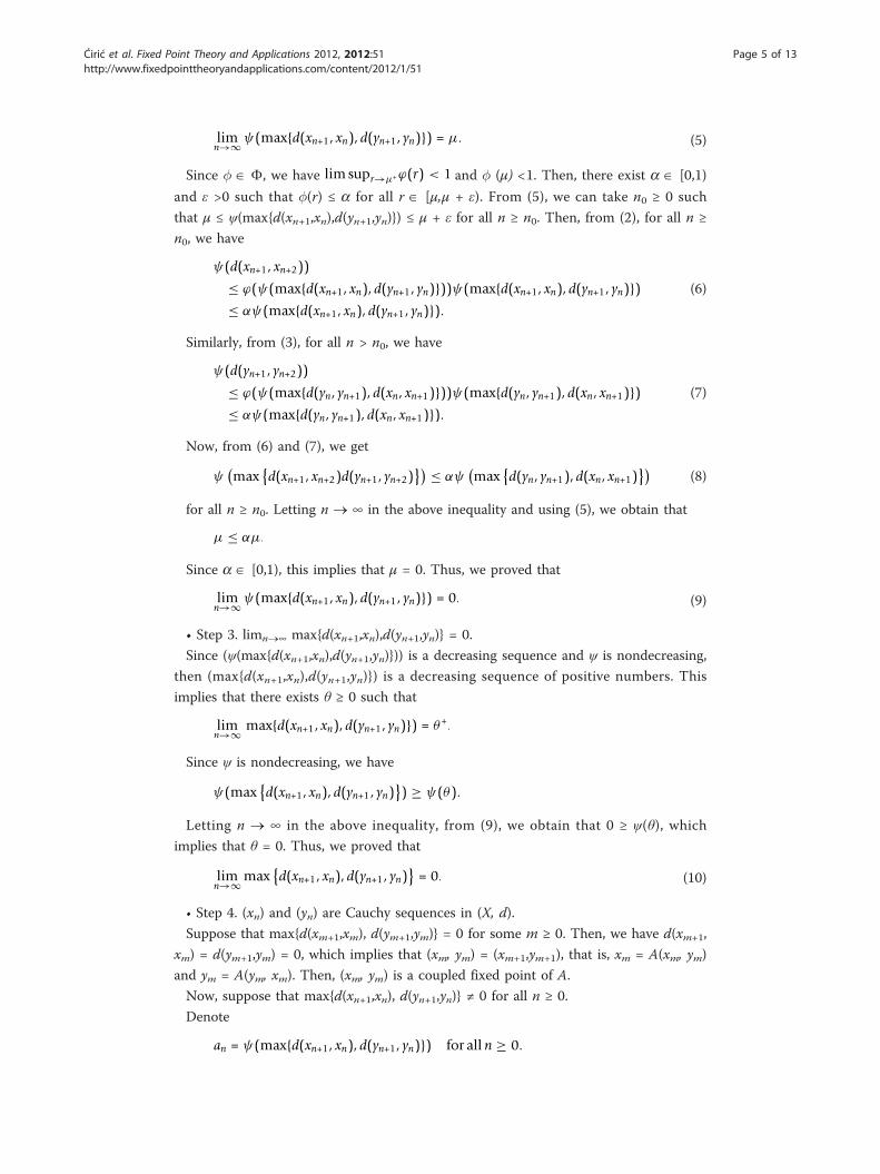
limn→∞ ψ(max{d(xn+1, xn), d(yn+1, yn)}) = μ. (5)

Since � Î F, we have lim supr→μ+ϕ(r) < 1 and � (μ) <1. Then, there exist a Î [0,1)

and ε >0 such that �(r) ≤ a for all r Î [μ,μ + ε). From (5), we can take n0 ≥ 0 such

that μ ≤ ψ(max{d(xn+1,xn),d(yn+1,yn)}) ≤ μ + ε for all n ≥ n0. Then, from (2), for all n ≥

n0, we have

ψ(d(xn+1, xn+2))

≤ ϕ(ψ(max{d(xn+1, xn), d(yn+1, yn)}))ψ(max{d(xn+1, xn), d(yn+1, yn)})≤ αψ(max{d(xn+1, xn), d(yn+1, yn)}).

(6)

Similarly, from (3), for all n > n0, we have

ψ(d(yn+1, yn+2))

≤ ϕ(ψ(max{d(yn, yn+1), d(xn, xn+1)}))ψ(max{d(yn, yn+1), d(xn, xn+1)})≤ αψ(max{d(yn, yn+1), d(xn, xn+1)}).

(7)

Now, from (6) and (7), we get

ψ(max

{d(xn+1, xn+2)d(yn+1, yn+2)

}) ≤ αψ(max

{d(yn, yn+1), d(xn, xn+1)

})(8)

for all n ≥ n0. Letting n ® ∞ in the above inequality and using (5), we obtain that

μ ≤ αμ.

Since a Î [0,1), this implies that μ = 0. Thus, we proved that

limn→∞ ψ(max{d(xn+1, xn), d(yn+1, yn)}) = 0. (9)

• Step 3. limn®∞ max{d(xn+1,xn),d(yn+1,yn)} = 0.

Since (ψ(max{d(xn+1,xn),d(yn+1,yn)})) is a decreasing sequence and ψ is nondecreasing,

then (max{d(xn+1,xn),d(yn+1,yn)}) is a decreasing sequence of positive numbers. This

implies that there exists θ ≥ 0 such that

limn→∞ max{d(xn+1, xn), d(yn+1, yn)}) = θ+.

Since ψ is nondecreasing, we have

ψ(max{d(xn+1, xn), d(yn+1, yn)

}) ≥ ψ(θ).

Letting n ® ∞ in the above inequality, from (9), we obtain that 0 ≥ ψ(θ), which

implies that θ = 0. Thus, we proved that

limn→∞max

{d(xn+1, xn), d(yn+1, yn)

}= 0. (10)

• Step 4. (xn) and (yn) are Cauchy sequences in (X, d).

Suppose that max{d(xm+1,xm), d(ym+1,ym)} = 0 for some m ≥ 0. Then, we have d(xm+1,

xm) = d(ym+1,ym) = 0, which implies that (xm, ym) = (xm+1,ym+1), that is, xm = A(xm, ym)

and ym = A(ym, xm). Then, (xm, ym) is a coupled fixed point of A.

Now, suppose that max{d(xn+1,xn), d(yn+1,yn)} ≠ 0 for all n ≥ 0.

Denote

an = ψ(max{d(xn+1, xn), d(yn+1, yn)}) for all n ≥ 0.


of 13

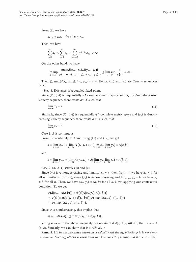
From (8), we have

an+1 ≤ αan for all n ≥ n0.

Then, we have

∞∑n=0

an ≤n0∑n=0

an +∞∑

n=n0+1

αn−n0an0 < ∞.

On the other hand, we have

lim supn→∞

max{d(xn+1, xn), d(yn+1, yn)}ψ(max{d(xn+1, xn), d(yn+1, yn)}) ≤ lim sup

s→0+

s

ψ(s)< ∞.

Then ∑n max{d(xn, xn+1),d(yn, yn+1)} < ∞. Hence, (xn) and (yn) are Cauchy sequences

in X.

• Step 5. Existence of a coupled fixed point.

Since (X, d, ≼) is sequentially ≼↕-complete metric space and (xn) is ≼-nondecreasingCauchy sequence, there exists aÎ X such that

limn→∞ xn = a. (11)

Similarly, since (X, d, ≼) is sequentially ≼↕-complete metric space and (yn) is ≼-noin-creasing Cauchy sequence, there exists b Î X such that

limn→∞ yn = b. (12)

Case 1. A is continuous.

From the continuity of A and using (11) and (12), we get

a = limn→∞ xn+1 = lim

n→∞A(xn, yn

)= A( lim

n→∞ xn, limn→∞ yn) = A(a, b)

and

b = limn→∞ yn+1 = lim

n→∞A(yn, xn

)= A( lim

n→∞ yn, limn→∞ xn) = A(b, a).

Case 2. (X, d, ≼) satisfies (i) and (ii).

Since (xn) is ≼-nondecreasing and limn®∞ xn = a, then from (i), we have xn ≼ a for

all n. Similarly, from (ii), since (yn) is ≼-nonincreasing and limn®∞ yn = b, we have yn≽ b for all n. Then, we have (xn, yn) ≼ (a, b) for all n. Now, applying our contractive

condition (1), we get

ψ(d(xn+1,A(a, b))) = ψ(d(A(xn, yn),A(a, b)))

≤ ϕ(ψ(max{d(xn, a), d(yn, b)}))ψ(max{d(xn, a), d(yn, b)})≤ ψ(max{d(xn, a), d(yn, b)}).

Since ψ is nondecreasing, this implies that

d(xn+1,A(a, b)) ≤ max{d(xn, a), d(yn, b)}.

letting n ® ∞ in the above inequality, we obtain that d(a, A(a, b)) ≤ 0, that is, a = A

(a, b). Similarly, we can show that b = A(b, a). □Remark 2.1 In our presented theorems we don’t need the hypothesis: ψ is lower semi-

continuous. Such hypothesis is considered in Theorem 1.7 of Gordji and Ramezani [14].


of 13

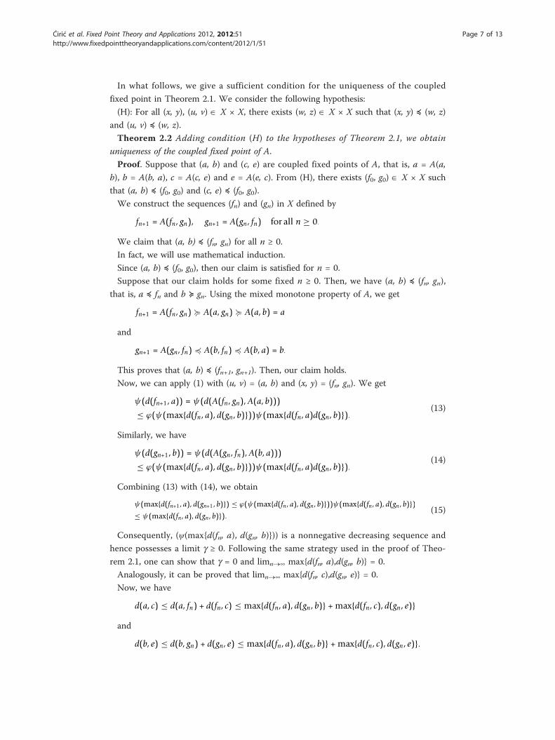
In what follows, we give a sufficient condition for the uniqueness of the coupled

fixed point in Theorem 2.1. We consider the following hypothesis:

(H): For all (x, y), (u, v) Î X × X, there exists (w, z) Î X × X such that (x, y) ≼ (w, z)

and (u, v) ≼ (w, z).

Theorem 2.2 Adding condition (H) to the hypotheses of Theorem 2.1, we obtain

uniqueness of the coupled fixed point of A.

Proof. Suppose that (a, b) and (c, e) are coupled fixed points of A, that is, a = A(a,

b), b = A(b, a), c = A(c, e) and e = A(e, c). From (H), there exists (f0, g0) Î X × X such

that (a, b) ≼ (f0, g0) and (c, e) ≼ (f0, g0).

We construct the sequences (fn) and (gn) in X defined by

fn+1 = A(fn, gn), gn+1 = A(gn, fn) for all n ≥ 0.

We claim that (a, b) ≼ (fn, gn) for all n ≥ 0.

In fact, we will use mathematical induction.

Since (a, b) ≼ (f0, g0), then our claim is satisfied for n = 0.

Suppose that our claim holds for some fixed n ≥ 0. Then, we have (a, b) ≼ (fn, gn),

that is, a ≼ fn and b ≽ gn. Using the mixed monotone property of A, we get

fn+1 = A(fn, gn) � A(a, gn) � A(a, b) = a

and

gn+1 = A(gn, fn) � A(b, fn) � A(b, a) = b.

This proves that (a, b) ≼ (fn+1, gn+1). Then, our claim holds.

Now, we can apply (1) with (u, v) = (a, b) and (x, y) = (fn, gn). We get

ψ(d(fn+1, a)) = ψ(d(A(fn, gn),A(a, b)))

≤ ϕ(ψ(max{d(fn, a), d(gn, b)}))ψ(max{d(fn, a)d(gn, b)}).(13)

Similarly, we have

ψ(d(gn+1, b)) = ψ(d(A(gn, fn),A(b, a)))

≤ ϕ(ψ(max{d(fn, a), d(gn, b)}))ψ(max{d(fn, a)d(gn, b)}).(14)

Combining (13) with (14), we obtain

ψ(max{d(fn+1, a), d(gn+1, b)}) ≤ ϕ(ψ(max{d(fn, a), d(gn, b)}))ψ(max{d(fn, a), d(gn, b)})≤ ψ(max{d(fn, a), d(gn, b)}). (15)

Consequently, (ψ(max{d(fn, a), d(gn, b)})) is a nonnegative decreasing sequence and

hence possesses a limit g ≥ 0. Following the same strategy used in the proof of Theo-

rem 2.1, one can show that g = 0 and limn®∞ max{d(fn, a),d(gn, b)} = 0.

Analogously, it can be proved that limn®∞ max{d(fn, c),d(gn, e)} = 0.

Now, we have

d(a, c) ≤ d(a, fn) + d(fn, c) ≤ max{d(fn, a), d(gn, b)} + max{d(fn, c), d(gn, e)}

and

d(b, e) ≤ d(b, gn) + d(gn, e) ≤ max{d(fn, a), d(gn, b)} + max{d(fn, c), d(gn, e)}.


of 13

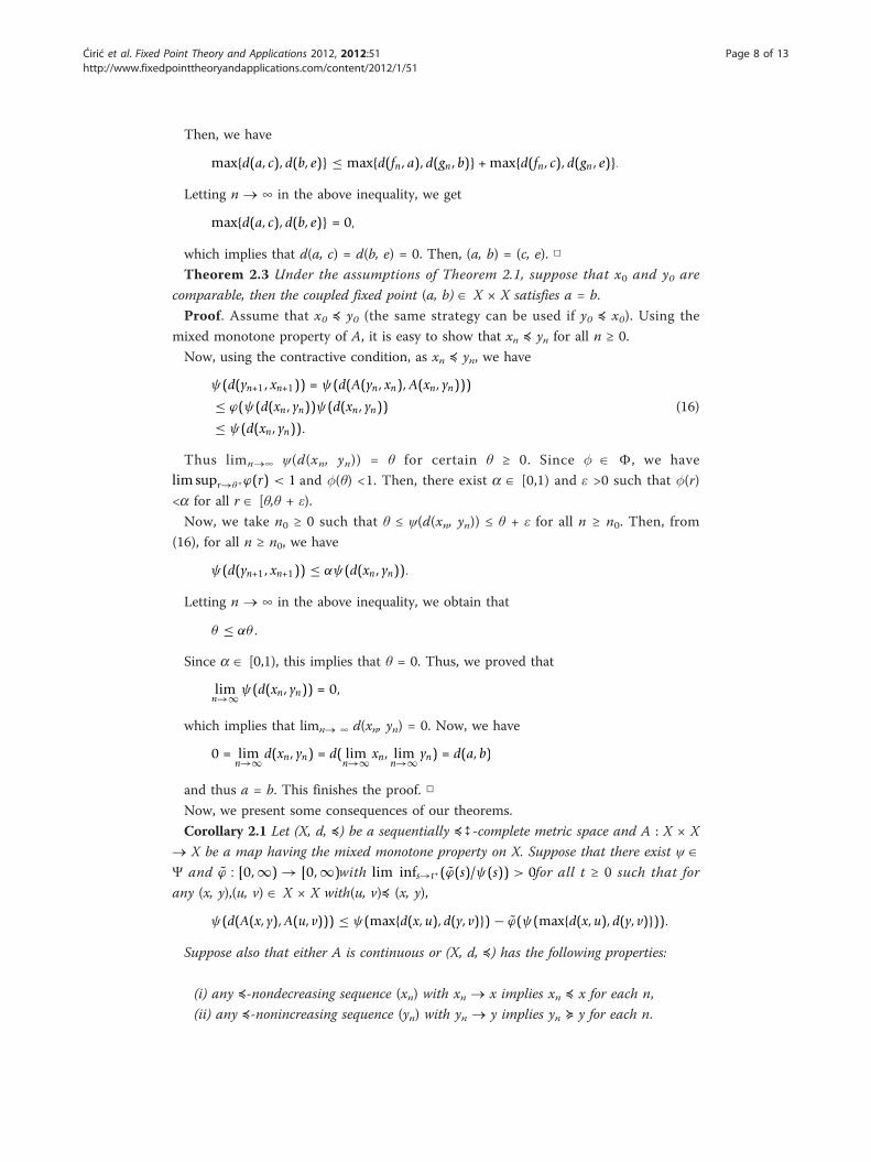
Then, we have

max{d(a, c), d(b, e)} ≤ max{d(fn, a), d(gn, b)} + max{d(fn, c), d(gn , e)}.

Letting n ® ∞ in the above inequality, we get

max{d(a, c), d(b, e)} = 0,

which implies that d(a, c) = d(b, e) = 0. Then, (a, b) = (c, e). □Theorem 2.3 Under the assumptions of Theorem 2.1, suppose that x0 and y0 are

comparable, then the coupled fixed point (a, b) Î X × X satisfies a = b.

Proof. Assume that x0 ≼ y0 (the same strategy can be used if y0 ≼ x0). Using the

mixed monotone property of A, it is easy to show that xn ≼ yn for all n ≥ 0.

Now, using the contractive condition, as xn ≼ yn, we have

ψ(d(yn+1, xn+1)) = ψ(d(A(yn, xn),A(xn, yn)))

≤ ϕ(ψ(d(xn, yn))ψ(d(xn, yn))

≤ ψ(d(xn, yn)).

(16)

Thus limn®∞ ψ(d(xn, yn)) = θ for certain θ ≥ 0. Since � Î F, we have

lim supr→θ+ϕ(r) < 1 and �(θ) <1. Then, there exist a Î [0,1) and ε >0 such that �(r)

<a for all r Î [θ,θ + ε).

Now, we take n0 ≥ 0 such that θ ≤ ψ(d(xn, yn)) ≤ θ + ε for all n ≥ n0. Then, from

(16), for all n ≥ n0, we have

ψ(d(yn+1, xn+1)) ≤ αψ(d(xn, yn)).

Letting n ® ∞ in the above inequality, we obtain that

θ ≤ αθ .

Since a Î [0,1), this implies that θ = 0. Thus, we proved that

limn→∞ ψ(d(xn, yn)) = 0,

which implies that limn® ∞ d(xn, yn) = 0. Now, we have

0 = limn→∞ d(xn, yn) = d( lim

n→∞ xn, limn→∞ yn) = d(a, b)

and thus a = b. This finishes the proof. □Now, we present some consequences of our theorems.

Corollary 2.1 Let (X, d, ≼) be a sequentially ≼↕-complete metric space and A : X × X

® X be a map having the mixed monotone property on X. Suppose that there exist ψ ÎΨ and ϕ̃ : [0,∞) → [0,∞)with lim infs→t+ (ϕ̃(s)/ψ(s)) > 0for all t ≥ 0 such that for

any (x, y),(u, v) Î X × X with(u, v)≼ (x, y),

ψ(d(A(x, y),A(u, v))) ≤ ψ(max{d(x, u), d(y, v)}) − ϕ̃(ψ(max{d(x, u), d(y, v)})).





of 13

If there exist x0, y0 Î X such that x0 ≼ A (x0, y0) and y0 ≽ A(y0, x0), then there exist a,


Proof. It follows immediately from Theorem 2.1 by considering ϕ(s) = 1 − ϕ̃(s)/ψ(s).

□Remark 2.2 Corollary 2.1 is an extension of Harjani et al. [[15], Theorems 2 and 3].


® X be a map having the mixed monotone property on X. Suppose that there exists a

nondecreasing function � : [0, ∞) ® [0, 1) such that for any (x, y), (u, v) Î X × X with

(u, v) ≼ (x, y),

d(A(x, y),A(u, v)) ≤ ϕ(2max{d(x, u), d(y, v)})max{d(x, u), d(y, v)}.




If there exist x0, y0 Î X such that x0 ≼ A(x0, y0) and y0 ≽ A(y0, x0), then there exist a,


Proof. It follows from Theorem 2.1 by considering ψ(s) = 2s □Remark 2.3 If � is nondecreasing, Corollary 2.2 generalizes Du [[13], Theorems 1.5

and 1.6].


® X be a map having the mixed monotone property on X. Suppose that there exists k Î[0, 1) such that for any (x, y),(u, v) Î X × X with (u, v) ≼ (x, y),

d(A(x, y),A(u, v)) ≤ kmax{d(x, u), d(y, v)}.




If there exist x0, y0 Î X such that x0 ≼ A(x0, y0) and y0 ≽ A(y0, x0), then there exist a,


Proof. It follows immediately from Corollary 2.2 by considering �(s) = k □Remark 2.4 Corollary 2.3 is a generalization of Bhaskar and Lakshmikantham [[11],

Theorems 2.1 and 2.2].

3 An applicationIn this section, we apply our main results to study the existence and uniqueness of

solution to the two-point boundary value problem⎧⎨⎩ −d2x

dt2(t) = f (t, x(t), x(t)), t ∈ [0, 1]

x(0) = x(1) = 0,(17)

where f : [0, 1] × ℝ × ℝ ® ℝ is a continuous function.

Previously we considered the space X = C(I, ℝ)(I = [0, 1]) of continuous functions

defined on I. Obviously, this space with the metric given by


of 13

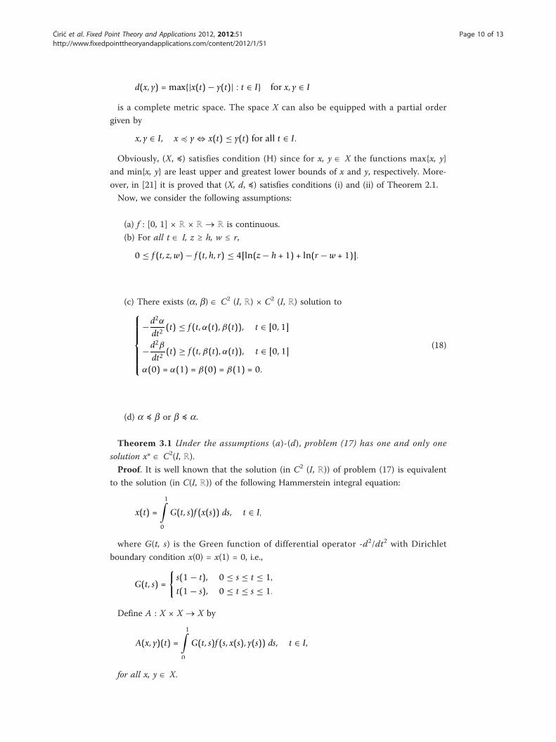
d(x, y) = max{|x(t) − y(t)| : t ∈ I} for x, y ∈ I

is a complete metric space. The space X can also be equipped with a partial order

given by

x, y ∈ I, x � y ⇔ x(t) ≤ y(t) for all t ∈ I.

Obviously, (X, ≼) satisfies condition (H) since for x, y Î X the functions max{x, y}

and min{x, y} are least upper and greatest lower bounds of x and y, respectively. More-

over, in [21] it is proved that (X, d, ≼) satisfies conditions (i) and (ii) of Theorem 2.1.

Now, we consider the following assumptions:

(a) f : [0, 1] × ℝ × ℝ ® ℝ is continuous.

(b) For all t Î I, z ≥ h, w ≤ r,

0 ≤ f (t, z,w) − f (t, h, r) ≤ 4[ln(z − h + 1) + ln(r − w + 1)].

(c) There exists (a, b) Î C2 (I, ℝ) × C2 (I, ℝ) solution to⎧⎪⎪⎪⎪⎪⎨⎪⎪⎪⎪⎪⎩

−d2αdt2

(t) ≤ f (t,α(t),β(t)), t ∈ [0, 1]

−d2βdt2

(t) ≥ f (t,β(t),α(t)), t ∈ [0, 1]

α(0) = α(1) = β(0) = β(1) = 0.

(18)

(d) a ≼ b or b ≼ a.

Theorem 3.1 Under the assumptions (a)-(d), problem (17) has one and only one

solution x* Î C2(I, ℝ).

Proof. It is well known that the solution (in C2 (I, ℝ)) of problem (17) is equivalent

to the solution (in C(I, ℝ)) of the following Hammerstein integral equation:

x(t) =

1∫0

G(t, s)f (x(s)) ds, t ∈ I,

where G(t, s) is the Green function of differential operator -d2/dt2 with Dirichlet

boundary condition x(0) = x(1) = 0, i.e.,

G(t, s) =

{s(1 − t), 0 ≤ s ≤ t ≤ 1,

t(1 − s), 0 ≤ t ≤ s ≤ 1.

Define A : X × X ® X by

A(x, y)(t) =

1∫0

G(t, s)f (s, x(s), y(s)) ds, t ∈ I,

for all x, y Î X.


of 13

From (b), it is clear that A has the mixed monotone property with respect to the par-

tial order ≼ in X.

Let x, y, u, v Î X such that x ≽ u and y ≼ υ. From (b), we have

d(A(x, y),A(u, v)) = supt∈I

|A(x, y)(t) − A(u, v)(t)|

= supt∈I

1∫0

G(t, s)[f (s, x(s), y(s)) − f (s, u(s), v(s))

]ds

≤ supt∈I

1∫0

4G(t, s)[ln(x(s) − u(s) + 1) + ln(v(s) − y(s) + 1)] ds

≤ (ln(d(x, u) + 1) + ln(d(y, v) + 1)) supt∈I

1∫0

4G(t, s) ds

≤⎛⎝sup

t∈I

1∫0

8G(t, s) ds

⎞⎠ ln (max{d(x, u), d(y, v)} + 1)

On the other hand, for all t Î I, we have

1∫0

G(t, s) ds =12t(1 − t),

which implies that

supt∈I

1∫0

G(t, s) ds =18.

Then, we get

d(A(x, y),A(u, v)) ≤ ln (max{d(x, u), d(y, v)} + 1).

This implies that

ln(d(A(x, y),A(u, v)) + 1

) ≤ ln(ln

(max{d(x, u), d(y, v)} + 1

)+ 1

)=ln

(ln

(max{d(x, u), d(y, v)} + 1

)+ 1

)ln

(max{d(x, u), d(y, v)} + 1

) ln(max{d(x, u), d(y, v)} + 1

).

Thus, the contractive condition (1) of Theorem (2.1) is satisfied with ψ(t) = ln(t + 1)

and �(t) = ψ(t)/t.

Now, let (a, b) Î C2 (I, ℝ) × C2 (I, ℝ) be a solution to (18). We will show that a ≼ A

(a, b) and b ≽ A(b, a). Indeed,

−α′′(s) ≤ f (s,α(s),β(s)), s ∈ [0, 1].

Multiplying by G(t, s), we get

1∫0

−α′′(s)G(t, s) ds ≤ A(α,β)(t), t ∈ [0, 1].


of 13

Then, for all t Î [0, 1], we have

−(1 − t)

1∫0

sα′′(s) ds − t

1∫t

(1 − s)α′′(s) ds ≤ A(α,β)(t).

Using an integration by parts, and since a(0) = a(1) = 0, for all t Î [0, 1], we get

−(1 − t)(tα′(t) − α(t)) − t(−(1 − t)α′(t) − α(t)) ≤ A(α,β)(t).

Thus, we have

α(t) ≤ A(α,β)(t), t ∈ [0, 1].

This implies that a ≼ A(a, b). Similarly, one can show that b ≽ A(b, a).Now, applying our Theorems 2.1 and 2.2, we deduce the existence of a unique (x, y)

Î X2 solution to x = A(x, y) and y = A(y, x). Moreover, from (d), and using Theorem

2.3, we get x = y. Thus, we proved that x* = x = y Î C2([0, 1], ℝ) is the unique solu-

tion to (17). □

AcknowledgementsL. Ćirić and B. Damjanović were supported by Grant No. 174025 of the Ministry of Science, Technology andDevelopment, Republic of Serbia.M. Jleli extends his appreciation to the Deanship of Scientific Research at King Saud University for funding the workthrough the research group project No RGP-VPP-087.

Author details1Faculty of Mechanical Engineering, University in Belgrade, Kraljice Marije 16, 11 000 Belgrade, Serbia 2Faculty ofAgriculture, University in Belgrade, Nemanjina 6, Belgrade, Serbia 3Department of Mathematics, King Saud University,Riyadh, Saudi Arabia

Authors’ contributionsAll authors contributed equally and significantly in writing this article. All authors read and approved the finalmanuscript.

Competing interestsThe authors declare that they have no competing interests.

Received: 27 October 2011 Accepted: 26 March 2012 Published: 26 March 2012

References1. Nadler, SB Jr: Multi-valued contraction mappings. Pacific J Math. 30, 475–488 (1969)2. Reich, S: Fixed points of contractive functions. Boll Un Mat Ital. 5, 26–42 (1972)3. Mizoguchi, N, Takahashi, W: Fixed point theorems for multivalued mappings on complete metric spaces. J Math Anal

Appl. 141, 177–188 (1989)4. Reich, S: Some problems and results in fixed point theory, in Topological Methods in Nonlinear Functional Analysis

(Toronto, Ont., 1982). In Contemp Math, vol. 21, pp. 179–187.American Mathematical Society, Providence, RI, USA (1983)5. Suzuki, T: Mizoguchi-Takahashi’s fixed point theorem is a real generalization of Nadler’s. J Math Anal Appl.

340(1):752–755 (2008)6. Amini-Harandi, A, O’Regan, D: Fixed point theorems for set-valued contraction type maps in metric spaces. Fixed Point

Theory Appl 2010, 7 (2010). Article ID 3901837. Agarwal, RP, El-Gebeily, MA, O’Regan, D: Generalized contractions in partially ordered metric spaces. Appl Anal.

87(1):109–116 (2008)8. Altun, I, Simsek, H: Some fixed point theorems on ordered metric spaces and application. Fixed Point Theory Appl

2010, 17 (2010). Article ID 6214929. Beg, I, Butt, AR: Fixed point for set-valued mappings satisfying an implicit relation in partially ordered metric spaces.

Nonlinear Anal. 71, 3699–3704 (2009)10. Berinde, V, Borcut, M: Tripled fixed point theorems for contractive type mappings in partially ordered metric spaces.

Nonlinear Anal. 74, 4889–4897 (2011)11. Bhaskar, TG, Lakshmikantham, V: Fixed point theorems in partially ordered metric spaces and applications. Nonlinear

Anal. 65(7):1379–1393 (2006)12. Ćirić, LjB, Cakić, N, Rajović, M, Ume, JS: Monotone generalized nonlinear contractions in partially ordered metric spaces.

Fixed Point Theory Appl 2008, 11 (2008). Article ID 13129413. Du, W-S: Coupled fixed point theorems for nonlinear contractions satisfied Mizoguchi-Takahashi’s condition in

quasiordered metric spaces. Fixed Point Theory Appl 2010, 9 (2010). Article ID 876372


of 13

14. Gordji, ME, Ramezani, M: A generalization of Mizoguchi and Takahashi’s theorem for single-valued mappings in partiallyordered metric spaces. Nonlinear Anal. 74, 4544–4549 (2011)

15. Harjani, J, López, B, Sadarangani, K: Fixed point theorems for mixed monotone operators and applications to integralequations. Nonlinear Anal. 74, 1749–1760 (2011)

16. Harjani, J, Sadarangani, K: Generalized contractions in partially ordered metric spaces and applications to ordinarydifferential equations. Nonlinear Anal. 72(3-4):1188–1197 (2010)

17. Jachymski, J: Equivalent conditions for generalized contractions on (ordered) metric spaces. Nonlinear Anal. 74, 768–774(2011)

18. Lakshmikantham, V, Ćirić, LjB: Coupled fixed point theorems for nonlinear contractions in partially ordered metricspaces. Nonlinear Anal. 70, 4341–4349 (2009)

19. Luong, NV, Thuan, NX: Coupled fixed points in partially ordered metric spaces and application. Nonlinear Anal. 74,983–992 (2011)

20. Nashine, HK, Samet, B, Kim, JK: Fixed point results for contractions involving generalized altering distances in orderedmetric spaces. Fixed Point Theory Appl. 2011, 5 (2011)

21. Nieto, JJ, López, RR: Contractive mapping theorems in partially ordered sets and applications to ordinary differentialequations. Order. 22, 223–239 (2005)

22. O’Regan, D, Petrusel, A: Fixed point theorems for generalized contractions in ordered metric spaces. J Math Anal Appl.341, 1241–1252 (2008)

23. Ran, ACM, Reurings, MCB: A fixed point theorem in partially ordered sets and some application to matrix equations.Proc Am Math Soc. 132, 1435–1443 (2004)

24. Samet, B: Coupled fixed point theorems for a generalized Meir-Keeler contraction in partially ordered metric spaces.Nonlinear Anal. 72, 4508–4517 (2010)

25. Samet, B, Vetro, C: Coupled fixed point theorems for multi-valued nonlinear contraction mappings in partially orderedmetric spaces. Nonlinear Anal. 74, 4260–4268 (2011)

26. Samet, B, Vetro, C, Vetro, P: Fixed point theorems for α - ψ-contractive type mappings. Nonlinear Anal. 75, 2154–2165(2012)

27. Turinici, M: Abstract comparison principles and multivariable Gronwall-Bellman inequalities. J Math Anal Appl. 117,100–127 (1986)

doi:10.1186/1687-1812-2012-51Cite this article as: Ćirić et al.: Coupled fixed point theorems for generalized Mizoguchi-Takahashi contractionswith applications. Fixed Point Theory and Applications 2012 2012:51.

Submit your manuscript to a journal and benefi t from:

7 Convenient online submission

7 Rigorous peer review

7 Immediate publication on acceptance

7 Open access: articles freely available online

7 High visibility within the fi eld

7 Retaining the copyright to your article

Submit your next manuscript at 7 springeropen.com


of 13

http://www.springeropen.com/

http://www.springeropen.com/

coupled fixed point theorems for generalized mizoguchi

Documents