coupled electromagnetic thermal analysis of ybco...

EUCAS 2015 preprint 2A-LS-P-04.14. Submitted to IEEE Trans. Appl. Supercond. for possible publication. S-P-04.14 1

Coupled Electromagnetic-Thermal Analysis of YBCO Bulk Magnets for the Excitation System of

Low-Speed Electric Generators J. Arnaud and P.J. Costa Branco

Abstract— This paper examines the use of YBCO HTS bulk

magnets when operating in the magnetic environment of low-

speed synchronous generators. A coupled electrothermal Comsol

model of bulk YBCOs is first developed, tested and

experimentally verified. Joule losses in the HTS magnet are then

studied when under AC magnetic fields with frequency and

amplitude ranges usually found in those generators. The YBCO

capability in maintaining its magnetization level when subjected

to those conditions was also analyzed since the objective is to

replace the permanent magnets currently used.

The conditions for which superconductivity is lost are studied

considering now the magnet submerged in liquid nitrogen. Using

the model developed, it was possible to observe temperature rise

effects in the superconductor and how temperature influences all

its parameters.

Index Terms— Superconducting generators, high temperature

superconductors, YBCO, HTS modelling,

I. INTRODUCTION UPERCONDUCTING power converters have been researchedsince the 1950s for applications where a high efficiency

and power density is required. The first approach was replacing copper coils by superconducting ones because they were able to carry large electric current densities without significant Joule losses. Initially, low critical temperature coils were used to generate the excitation field of synchronous machines, but it did not support large variations of external magnetic fields. The appearing of AC superconducting wires however allowed fully superconducting synchronous machines [1]. Another approach has been using conventional iron-core machines with the insertion of high temperature superconductors (HTSs). In reluctance synchronous machines, for example, the rotor moves towards a position favoring a value of maximum magnetic flux. Electromagnetic torque produced by these machines is proportional to the difference of d and q axis inductances. It is possible to augment this difference by placing a ferromagnetic material in one axis and a bulk HTS operating as a magnetic shield in the other axis, therefore increasing the torque as proposed in [2-3].

Recently, many innovative structures using HTSs have been presented for their property of large current density transport

This work was supported by FCT, through IDMEC, under LAETA, project UID/EMS/50022/2013.

J. Arnaud is with the Electrical and Computers Engineering Department, Instituto Superior Técnico, Universidade de Lisboa, Portugal.

P.J. Costa Branco is with LAETA, IDMEC, Instituto Superior Técnico, Universidade de Lisboa, Lisboa, Portugal.: (e-mail: [email protected]). Corresponding author.

and/or quantum levitation. An example which exploits the magnetic behavior of bulk HTSs is the hysteresis machine, which develops its electromagnetic torque using their hysteresis characteristic [4]. Another usual approach consists in using HTS coils that have the main advantage of larger current densities, ranging from 10 to 1000 times that of copper. They also allow obtaining larger air-gap magnetic fields without any active iron, tolerating higher armature loading and, when replacing all or even part of copper coils, they generally increases machine efficiency.

Electromechanical power converters using HTS bulks have gained significant attention recently [5-6]. By exploiting their flux trapping and/or flux shielding capabilities, different electrical machines design can be achieved. Trapping large fields in HTS bulks using the novel pulsed-field magnetization technique [4] [7-10] has opened the appearing of HTS bulk magnets that can trap nearly 2T at 77K. This allows surpassing neodymium permanent magnets (NdFeB) field in about 40% and the use of HTS bulk magnets as the excitation system of electrical machines. However, the liquid nitrogen cooling system (including the cryostat) can minimize the advantages of using this type of HTS electrical machine. Problems such as transporting the cryogenic coolant to the superconductors, determining the cryostat location (either in the rotor and/or in a fixed stator, or even surrounding the whole machine), and determining the core material (air-core vs iron-core machines or hybrid topologies) are all open topics that show it is not yet evident which design is more acceptable.

HTS machines are still in development. Recently, a 1 MW HTS synchronous motor has been developed in China [5]. Also, projects for synchronous generators for wind power generation have been conducted such as a 12 MW LTS generator [11] and a 10 MW salient-pole HTS generator [1]. Superconducting linear generators were also constructed in the last few years using not only HTS coils but also HTS bulks [2-3].

This paper includes the study, modeling and analysis of the process of magnetization in bulk HTSs, verification of the YBCO capability in maintaining its magnetization level when subjected to time-variant magnetic fields, including also an analysis of the advantages and disadvantages of using YBCO magnets in low-speed synchronous generators. Expected accomplishments include a coupled electrothermal Comsol model for simulation of bulk superconductors when submerged in liquid nitrogen, the determination of a set of

S

IEEE/CSC & ESAS SUPERCONDUCTIVITY NEWS FORUM (global edition), January 2016.

2

parameters and their characteristics to describe the behavior of YBCO bulk superconductors in a magnetic field confinement (in our case a synchronous generator),.

II. ELECTROMAGNETIC AND THERMAL HTS MODELING

A. Electromagnetic modelling It was based in the 2D H-formulation model presented in [2]. The magnetic field is applied along the x-y plane, so the current density and electric field will only have a component in z-direction. By applying Ampère’s Law, and assuming that Maxwell’s addition (the electric field derivative) is in this case negligible (quasi-static regime), the current density and the electric field in the superconductor in z-direction can be obtained by (1) and (2), respectively. 𝐽𝑠𝑐_𝑧 =

𝜕𝐻𝑦

𝜕𝑥−

𝜕𝐻𝑥

𝜕𝑦 𝑒𝑧⃗⃗ ⃗ (1)

𝐸𝑠𝑐_𝑧 = 𝐸0 (

𝜕𝐻𝑦

𝜕𝑥−

𝜕𝐻𝑥𝜕𝑦

𝐽𝑐(𝐵))

𝑛

𝑒𝑧⃗⃗ ⃗ (2)

Substituting (1-2) in Faraday’s Law gives (3) where 𝜇𝑟 isconsidered to be equal to 1.

{𝜕(𝐸𝑠𝑐_𝑧) 𝜕𝑦⁄ = −𝜇0𝜇𝑟

𝜕𝐻𝑥

𝜕𝑡

−𝜕(𝐸𝑠𝑐_𝑧) 𝜕𝑥⁄ = −𝜇0𝜇𝑟𝜕𝐻𝑦

𝜕𝑡

(3)

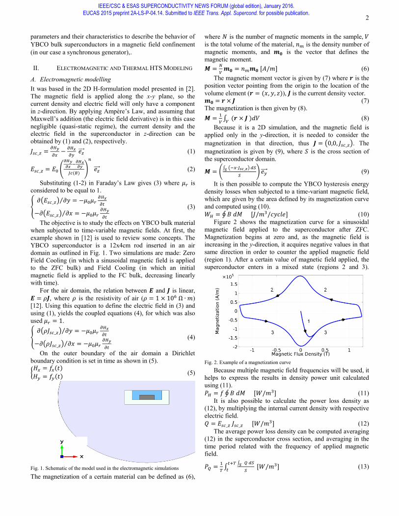
The objective is to study the effects on YBCO bulk material when subjected to time-variable magnetic fields. At first, the example shown in [12] is used to review some concepts. The YBCO superconductor is a 12x4cm rod inserted in an air domain as outlined in Fig. 1. Two simulations are made: Zero Field Cooling (in which a sinusoidal magnetic field is applied to the ZFC bulk) and Field Cooling (in which an initial magnetic field is applied to the FC bulk, decreasing linearly with time).

For the air domain, the relation between 𝑬 and 𝑱 is linear, 𝑬 = 𝜌𝑱, where 𝜌 is the resistivity of air (𝜌 = 1 × 106 Ω ∙ 𝑚)[12]. Using this equation to define the electric field in (3) and using (1), yields the coupled equations (4), for which was also used 𝜇𝑟 = 1.

{𝜕(𝜌𝐽𝑠𝑐_𝑧) 𝜕𝑦⁄ = −𝜇0𝜇𝑟

𝜕𝐻𝑥

𝜕𝑡

−𝜕(𝜌𝐽𝑠𝑐_𝑧) 𝜕𝑥⁄ = −𝜇0𝜇𝑟𝜕𝐻𝑦

𝜕𝑡

(4)

On the outer boundary of the air domain a Dirichlet boundary condition is set in time as shown in (5).

{𝐻𝑥 = 𝑓𝑥(𝑡)

𝐻𝑦 = 𝑓𝑦(𝑡)(5)

The magnetization of a certain material can be defined as (6),

where 𝑁 is the number of magnetic moments in the sample, 𝑉 is the total volume of the material, 𝑛𝑚 is the density number ofmagnetic moments, and 𝒎𝟎 is the vector that defines themagnetic moment. 𝑴 =

𝑁

𝑉𝒎𝟎 = 𝑛𝑚𝒎𝟎 [𝐴/𝑚] (6)

The magnetic moment vector is given by (7) where 𝒓 is the position vector pointing from the origin to the location of the volume element (𝒓 = (𝑥, 𝑦, 𝑧)), 𝑱 is the current density vector. 𝒎𝟎 = 𝒓 × 𝑱 (7) The magnetization is then given by (8). 𝑴 =

1

𝑉∫ (𝒓 × 𝑱 )𝑑𝑉𝑉

(8) Because it is a 2D simulation, and the magnetic field is

applied only in the y-direction, it is needed to consider the magnetization in that direction, thus 𝑱 = (0,0, 𝐽𝑠𝑐_𝑧). Themagnetization is given by (9), where 𝑆 is the cross section of the superconductor domain.

𝑴 = (∫ (−𝑥∙𝐽𝑠𝑐_𝑧) 𝑑𝑆𝑆

𝑆) 𝑒𝑦⃗⃗⃗⃗ (9)

It is then possible to compute the YBCO hysteresis energy density losses when subjected to a time-variant magnetic field, which are given by the area defined by its magnetization curve and computed using (10). 𝑊𝐻 = ∮𝐵 𝑑𝑀 [𝐽/𝑚3/𝑐𝑦𝑐𝑙𝑒] (10)

Figure 2 shows the magnetization curve for a sinusoidal magnetic field applied to the superconductor after ZFC. Magnetization begins at zero and, as the magnetic field is increasing in the y-direction, it acquires negative values in that same direction in order to counter the applied magnetic field (region 1). After a certain value of magnetic field applied, the superconductor enters in a mixed state (regions 2 and 3).

Because multiple magnetic field frequencies will be used, it helps to express the results in density power unit calculated using (11). 𝑃𝐻 = 𝑓 ∮𝐵 𝑑𝑀 [𝑊/𝑚3] (11)

It is also possible to calculate the power loss density as (12), by multiplying the internal current density with respective electric field. 𝑄 = 𝐸𝑠𝑐_𝑧 𝐽𝑠𝑐_𝑧 [𝑊/𝑚3] (12)

The average power loss density can be computed averaging (12) in the superconductor cross section, and averaging in the time period related with the frequency of applied magnetic field.

𝑃𝑄 =1

𝑇∫

∫ 𝑄𝑆 𝑑𝑆

𝑆

𝑡+𝑇

𝑡 [𝑊/𝑚3] (13)

Fig. 2. Example of a magnetization curve

Fig. 1. Schematic of the model used in the electromagnetic simulations

SUPERCONDUCTOR

AIR

IEEE/CSC & ESAS SUPERCONDUCTIVITY NEWS FORUM (global edition), January 2016.EUCAS 2015 preprint 2A-LS-P-04.14. Submitted to IEEE Trans. Appl. Supercond. for possible publication.

3

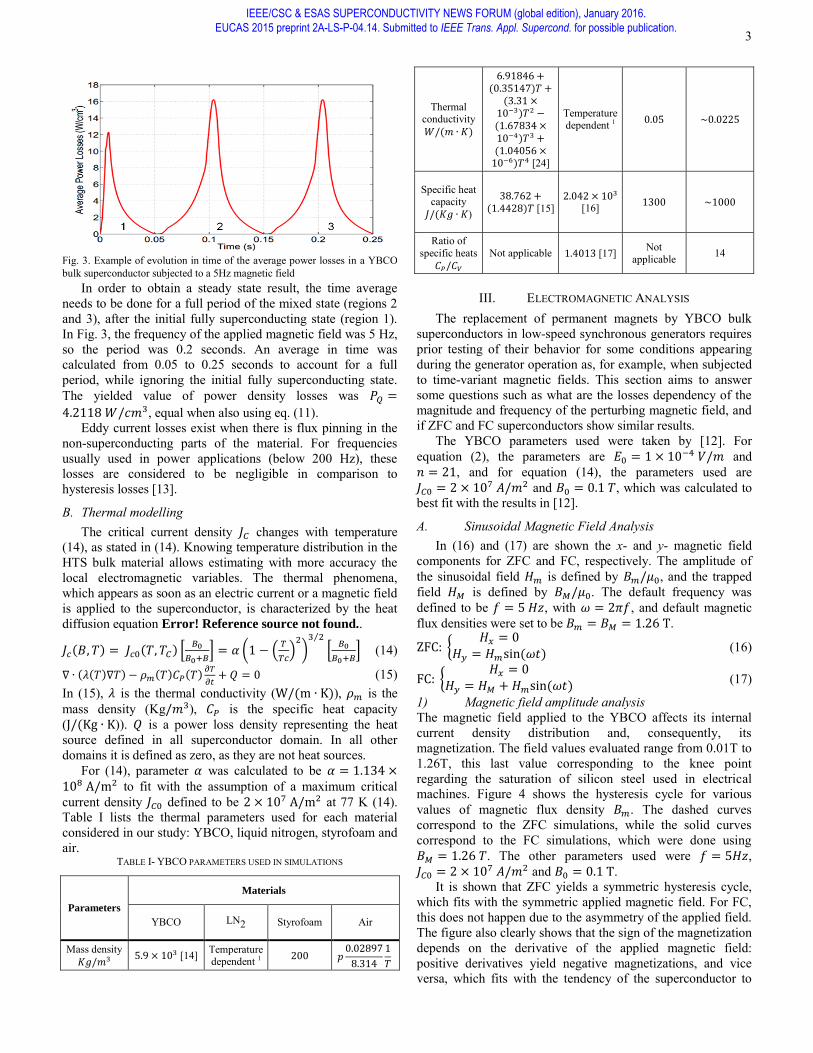
In order to obtain a steady state result, the time average needs to be done for a full period of the mixed state (regions 2 and 3), after the initial fully superconducting state (region 1). In Fig. 3, the frequency of the applied magnetic field was 5 Hz, so the period was 0.2 seconds. An average in time was calculated from 0.05 to 0.25 seconds to account for a full period, while ignoring the initial fully superconducting state. The yielded value of power density losses was 𝑃𝑄 =

4.2118 𝑊/𝑐𝑚3, equal when also using eq. (11).Eddy current losses exist when there is flux pinning in the

non-superconducting parts of the material. For frequencies usually used in power applications (below 200 Hz), these losses are considered to be negligible in comparison to hysteresis losses [13].

B. Thermal modelling The critical current density 𝐽𝐶 changes with temperature

(14), as stated in (14). Knowing temperature distribution in the HTS bulk material allows estimating with more accuracy the local electromagnetic variables. The thermal phenomena, which appears as soon as an electric current or a magnetic field is applied to the superconductor, is characterized by the heat diffusion equation Error! Reference source not found..

𝐽𝑐(𝐵, 𝑇) = 𝐽𝑐0(𝑇, 𝑇𝐶) [𝐵0

𝐵0+𝐵] = 𝛼 (1 − (

𝑇

𝑇𝑐)2

)3 2⁄

[𝐵0

𝐵0+𝐵] (14)

∇ ∙ (𝜆(𝑇)∇𝑇) − 𝜌𝑚(𝑇)𝐶𝑃(𝑇)𝜕𝑇

𝜕𝑡+ 𝑄 = 0 (15)

In (15), 𝜆 is the thermal conductivity (W/(m ∙ K)), 𝜌𝑚 is themass density (Kg/𝑚3), 𝐶𝑃 is the specific heat capacity(J/(Kg ∙ K)). 𝑄 is a power loss density representing the heat source defined in all superconductor domain. In all other domains it is defined as zero, as they are not heat sources.

For (14), parameter 𝛼 was calculated to be 𝛼 = 1.134 ×108 A/m2 to fit with the assumption of a maximum criticalcurrent density 𝐽𝐶0 defined to be 2 × 107 A/m2 at 77 K (14).Table I lists the thermal parameters used for each material considered in our study: YBCO, liquid nitrogen, styrofoam and air.

TABLE I- YBCO PARAMETERS USED IN SIMULATIONS

Parameters

Materials

YBCO LN2 Styrofoam Air

Mass density 𝐾𝑔/𝑚3 5.9 × 103 [14] Temperature

dependent 1 200 𝑝0.02897

8.314

1

𝑇

Thermal conductivity 𝑊/(𝑚 ∙ 𝐾)

6.91846 +(0.35147)𝑇 +

(3.31 ×10−3)𝑇2 −(1.67834 ×10−4)𝑇3 +(1.04056 ×10−6)𝑇4 [24]

Temperature dependent 1 0.05 ~0.0225

Specific heat capacity

𝐽/(𝐾𝑔 ∙ 𝐾)

38.762 +(1.4428)𝑇 [15]

2.042 × 103 [16] 1300 ~1000

Ratio of specific heats

𝐶𝑃/𝐶𝑉

Not applicable 1.4013 [17] Not applicable 14

III. ELECTROMAGNETIC ANALYSIS

The replacement of permanent magnets by YBCO bulk superconductors in low-speed synchronous generators requires prior testing of their behavior for some conditions appearing during the generator operation as, for example, when subjected to time-variant magnetic fields. This section aims to answer some questions such as what are the losses dependency of the magnitude and frequency of the perturbing magnetic field, and if ZFC and FC superconductors show similar results.

The YBCO parameters used were taken by [12]. For equation (2), the parameters are 𝐸0 = 1 × 10−4 𝑉/𝑚 and𝑛 = 21, and for equation (14), the parameters used are 𝐽𝐶0 = 2 × 107 𝐴/𝑚2 and 𝐵0 = 0.1 𝑇, which was calculated tobest fit with the results in [12].

A. Sinusoidal Magnetic Field Analysis In (16) and (17) are shown the x- and y- magnetic field

components for ZFC and FC, respectively. The amplitude of the sinusoidal field 𝐻𝑚 is defined by 𝐵𝑚/𝜇0, and the trappedfield 𝐻𝑀 is defined by 𝐵𝑀/𝜇0. The default frequency wasdefined to be 𝑓 = 5 𝐻𝑧, with 𝜔 = 2𝜋𝑓, and default magnetic flux densities were set to be 𝐵𝑚 = 𝐵𝑀 = 1.26 T.

ZFC: {𝐻𝑥 = 0

𝐻𝑦 = 𝐻𝑚sin (𝜔𝑡) (16)

FC: {𝐻𝑥 = 0

𝐻𝑦 = 𝐻𝑀 + 𝐻𝑚sin (𝜔𝑡) (17)

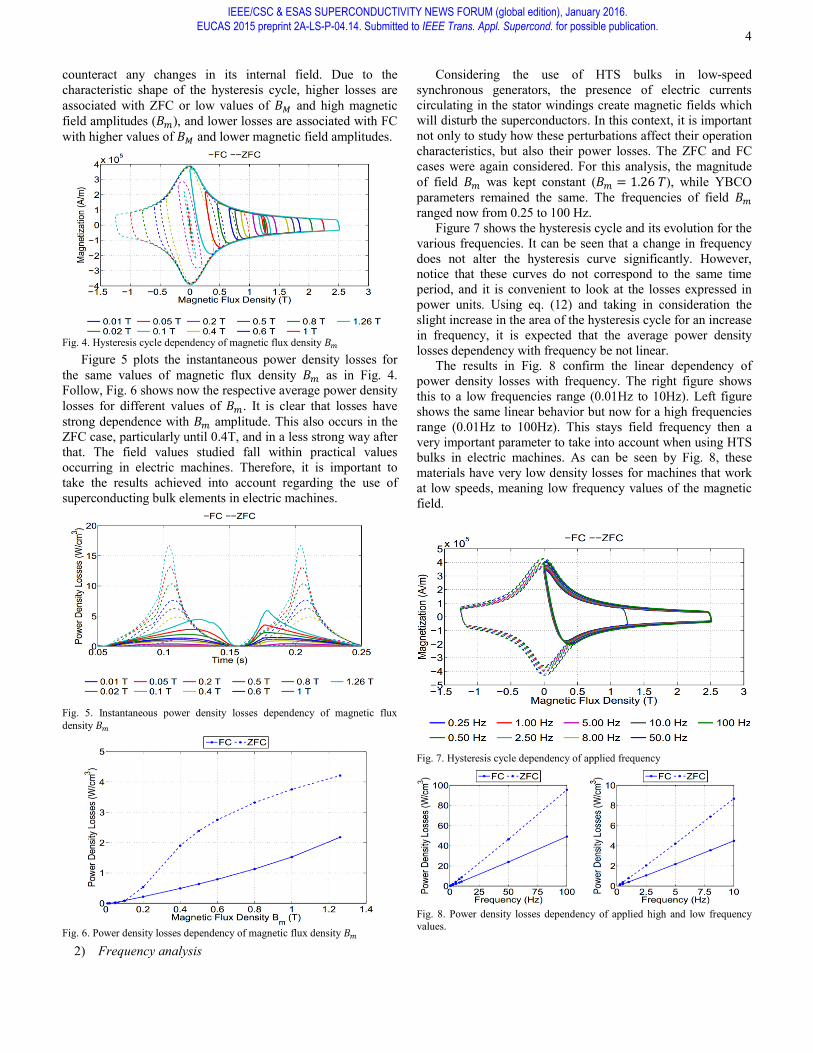
1) Magnetic field amplitude analysis The magnetic field applied to the YBCO affects its internal current density distribution and, consequently, its magnetization. The field values evaluated range from 0.01T to 1.26T, this last value corresponding to the knee point regarding the saturation of silicon steel used in electrical machines. Figure 4 shows the hysteresis cycle for various values of magnetic flux density 𝐵𝑚. The dashed curvescorrespond to the ZFC simulations, while the solid curves correspond to the FC simulations, which were done using 𝐵𝑀 = 1.26 𝑇. The other parameters used were 𝑓 = 5𝐻𝑧,𝐽𝐶0 = 2 × 107 𝐴/𝑚2 and 𝐵0 = 0.1 T.

It is shown that ZFC yields a symmetric hysteresis cycle, which fits with the symmetric applied magnetic field. For FC, this does not happen due to the asymmetry of the applied field. The figure also clearly shows that the sign of the magnetization depends on the derivative of the applied magnetic field: positive derivatives yield negative magnetizations, and vice versa, which fits with the tendency of the superconductor to

Fig. 3. Example of evolution in time of the average power losses in a YBCO bulk superconductor subjected to a 5Hz magnetic field


4

counteract any changes in its internal field. Due to the characteristic shape of the hysteresis cycle, higher losses are associated with ZFC or low values of 𝐵𝑀 and high magneticfield amplitudes (𝐵𝑚), and lower losses are associated with FCwith higher values of 𝐵𝑀 and lower magnetic field amplitudes.

Figure 5 plots the instantaneous power density losses for the same values of magnetic flux density 𝐵𝑚 as in Fig. 4.Follow, Fig. 6 shows now the respective average power density losses for different values of 𝐵𝑚. It is clear that losses havestrong dependence with 𝐵𝑚 amplitude. This also occurs in theZFC case, particularly until 0.4T, and in a less strong way after that. The field values studied fall within practical values occurring in electric machines. Therefore, it is important to take the results achieved into account regarding the use of superconducting bulk elements in electric machines.

2) Frequency analysis

Considering the use of HTS bulks in low-speed synchronous generators, the presence of electric currents circulating in the stator windings create magnetic fields which will disturb the superconductors. In this context, it is important not only to study how these perturbations affect their operation characteristics, but also their power losses. The ZFC and FC cases were again considered. For this analysis, the magnitude of field 𝐵𝑚 was kept constant (𝐵𝑚 = 1.26 𝑇), while YBCOparameters remained the same. The frequencies of field 𝐵𝑚

ranged now from 0.25 to 100 Hz. Figure 7 shows the hysteresis cycle and its evolution for the

various frequencies. It can be seen that a change in frequency does not alter the hysteresis curve significantly. However, notice that these curves do not correspond to the same time period, and it is convenient to look at the losses expressed in power units. Using eq. (12) and taking in consideration the slight increase in the area of the hysteresis cycle for an increase in frequency, it is expected that the average power density losses dependency with frequency be not linear.

The results in Fig. 8 confirm the linear dependency of power density losses with frequency. The right figure shows this to a low frequencies range (0.01Hz to 10Hz). Left figure shows the same linear behavior but now for a high frequencies range (0.01Hz to 100Hz). This stays field frequency then a very important parameter to take into account when using HTS bulks in electric machines. As can be seen by Fig. 8, these materials have very low density losses for machines that work at low speeds, meaning low frequency values of the magnetic field.

Fig. 7. Hysteresis cycle dependency of applied frequency

Fig. 6. Power density losses dependency of magnetic flux density 𝐵𝑚

Fig. 5. Instantaneous power density losses dependency of magnetic flux density 𝐵𝑚

Fig. 4. Hysteresis cycle dependency of magnetic flux density 𝐵𝑚

Fig. 8. Power density losses dependency of applied high and low frequency values.


5

B. Field Cooling Transient Analysis for Trapped Field This section studies some transient tests with the objective

of magnetizing the superconductor by looking at the value of the magnetic flux density trapped, and examining which parameters will be more important to increase its value.

An external field is applied, decreasing linearly from an initial value 𝐻𝑀0, defined by 𝐵𝑀0/𝜇0, to zero during aspecified time interval 𝑃. The Dirichlet boundary condition is set up as (18).

{𝐻𝑥 = 0

𝐻𝑦 = 𝐻𝑀0 −𝐻𝑀

𝑃𝑡, (0 ≤ 𝑡 ≤ 𝑃)

(18)

Some cases were studied: the initial applied magnetic flux density 𝐵𝑀0, the slope of applied field (by varying 𝑃), themaximum critical current density 𝐽𝐶0, parameter 𝐵0, thegeometric dimensions of the superconductor (specifically its width), and a long term analysis was also simulated where it is verified the influence of a small amplitude sinusoidal field applied after removing the initial field (like a small field perturbation). However, due to space restrictions, only the most significant one are presented. Simulation parameters used were 𝐵𝑀0 = 0.05 𝑇, 𝑃 = 0.05 𝑠, 𝐽

𝐶0= 2 × 107𝐴/𝑚2

and 𝐵0 = 0.1 𝑇.1) The initial applied field 𝐵𝑀0 analysis

The evolution of the trapped magnetic flux density is plotted in Fig. 9. It shows the maximum 𝐵 value in the upper boundary of the superconductor. Results indicate that the 𝐵𝑀0

value does not significantly affect the maximum trapped field for 𝐵𝑀0 values higher than 0.25 T. For lower values, thetrapped field stayed approximately constant and equal to applied field 𝐵𝑀0.

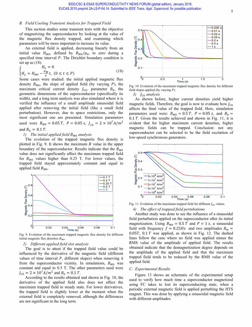
2) Different applied field slot analysisThe goal is to attest if the trapped field value could be

influenced by the derivative of the magnetic field (different values of time interval 𝑃, different slopes) when removing it from the superconductor vicinity. In simulations, 𝐵𝑀0 wasconstant and equal to 0.5 T. The other parameters used were 𝐽𝐶0 = 2 × 107𝐴/𝑚2 and 𝐵0 = 0.1 𝑇.

According to the results obtained and shown in Fig. 10, the derivative of the applied field also does not affect the maximum trapped field in steady state. For lower derivatives, the trapped field is slightly lower at the moment when the external field is completely removed, although the differences are not significant in the long term.

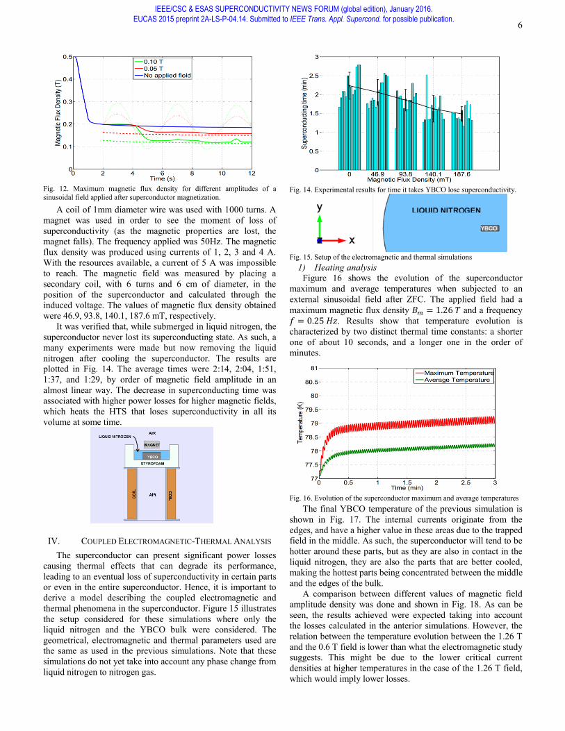
3) 𝐽𝐶0 analysisAs shown before, higher current densities yield higher

magnetic fields. Therefore, the goal is now to evaluate how 𝐽𝐶0

affects the final value of the trapped field. Here, simulation parameters used were: 𝐵𝑀0 = 0.5 𝑇, 𝑃 = 0.05 𝑠, and 𝐵0 =0.1 𝑇. Given the results achieved and shown in Fig. 11, it is evident that for higher maximum current densities, higher magnetic fields can be trapped. Conclusion: not any superconductor can be selected to be the field excitation of low-speed synchronous generators.

4) The effect of trapped field pertubationsAnother study was done to see the influence of a sinusoidal

field perturbation applied on the superconductor after its initial magnetization. Using 𝐵𝑀0 = 0.5 𝑇 and 𝑃 = 1 𝑠, a sinusoidalfield with frequency 𝑓 = 0.25𝐻𝑧 and two amplitudes 𝐵𝑚 =0.05𝑇, 0.1 𝑇 was applied, as shown in Fig. 12. The dashed lines follow the case where no field was applied minus the RMS value of the amplitude of applied field. The results obtained indicate that the demagnetization degree depends on the amplitude of the applied field and that the maximum trapped field tends to be reduced by the RMS value of the applied field.

C. Experimental Results Figure 13 shows an schematic of the experimental setup

used to verify how much time a superconductor magnetized using FC takes to lost its superconducting state, when a periodic external magnetic field is applied perturbing the HTS magnet. This was done by applying a sinusoidal magnetic field with different amplitudes.

Fig. 9. Evolution of the maximum trapped magnetic flux density for different initial magnetic flux densities 𝐵𝑀0.

Fig. 10. Evolution of the maximum trapped magnetic flux density for different field slopes applied (by varying 𝑃).

Fig. 11. Evolution of the maximum trapped field for different 𝐽𝐶0 values.


6

A coil of 1mm diameter wire was used with 1000 turns. A magnet was used in order to see the moment of loss of superconductivity (as the magnetic properties are lost, the magnet falls). The frequency applied was 50Hz. The magnetic flux density was produced using currents of 1, 2, 3 and 4 A. With the resources available, a current of 5 A was impossible to reach. The magnetic field was measured by placing a secondary coil, with 6 turns and 6 cm of diameter, in the position of the superconductor and calculated through the induced voltage. The values of magnetic flux density obtained were 46.9, 93.8, 140.1, 187.6 mT, respectively.

It was verified that, while submerged in liquid nitrogen, the superconductor never lost its superconducting state. As such, a many experiments were made but now removing the liquid nitrogen after cooling the superconductor. The results are plotted in Fig. 14. The average times were 2:14, 2:04, 1:51, 1:37, and 1:29, by order of magnetic field amplitude in an almost linear way. The decrease in superconducting time was associated with higher power losses for higher magnetic fields, which heats the HTS that loses superconductivity in all its volume at some time.

IV. COUPLED ELECTROMAGNETIC-THERMAL ANALYSIS

The superconductor can present significant power losses causing thermal effects that can degrade its performance, leading to an eventual loss of superconductivity in certain parts or even in the entire superconductor. Hence, it is important to derive a model describing the coupled electromagnetic and thermal phenomena in the superconductor. Figure 15 illustrates the setup considered for these simulations where only the liquid nitrogen and the YBCO bulk were considered. The geometrical, electromagnetic and thermal parameters used are the same as used in the previous simulations. Note that these simulations do not yet take into account any phase change from liquid nitrogen to nitrogen gas.

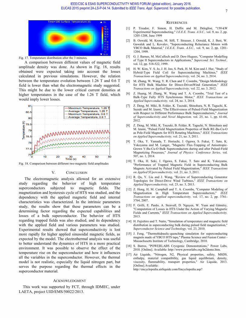
1) Heating analysisFigure 16 shows the evolution of the superconductor

maximum and average temperatures when subjected to an external sinusoidal field after ZFC. The applied field had a maximum magnetic flux density 𝐵𝑚 = 1.26 𝑇 and a frequency𝑓 = 0.25 𝐻𝑧. Results show that temperature evolution is characterized by two distinct thermal time constants: a shorter one of about 10 seconds, and a longer one in the order of minutes.

The final YBCO temperature of the previous simulation is shown in Fig. 17. The internal currents originate from the edges, and have a higher value in these areas due to the trapped field in the middle. As such, the superconductor will tend to be hotter around these parts, but as they are also in contact in the liquid nitrogen, they are also the parts that are better cooled, making the hottest parts being concentrated between the middle and the edges of the bulk.

A comparison between different values of magnetic field amplitude density was done and shown in Fig. 18. As can be seen, the results achieved were expected taking into account the losses calculated in the anterior simulations. However, the relation between the temperature evolution between the 1.26 T and the 0.6 T field is lower than what the electromagnetic study suggests. This might be due to the lower critical current densities at higher temperatures in the case of the 1.26 T field, which would imply lower losses.

Fig. 12. Maximum magnetic flux density for different amplitudes of a sinusoidal field applied after superconductor magnetization.

Fig. 13. Schematic of the lab experiment

Fig. 14. Experimental results for time it takes YBCO lose superconductivity.

Fig. 15. Setup of the electromagnetic and thermal simulations

Fig. 16. Evolution of the superconductor maximum and average temperatures


7

A comparison between different values of magnetic field amplitude density was done. As shown in Fig. 18, results obtained were expected taking into account the losses calculated in previous simulations. However, the relation between the temperature evolution between 1.26 T and 0.6 T field is lower than what the electromagnetic study suggested. This might be due to the lower critical current densities at higher temperatures in the case of the 1.26 T field, which would imply lower losses.

V. CONCLUSION The electromagnetic analysis allowed for an extensive

study regarding the behavior of high temperature superconductors subjected to magnetic fields. The magnetization and hysteresis cycle of HTS was studied, and the dependency with the applied magnetic field and internal characteristics was characterized. In the intrinsic parameters study, the results show that these parameters can be a determining factor regarding the expected capabilities and losses of a bulk superconductor. The behavior of HTS regarding trapped fields was also studied, and its dependency with the applied field and various parameters was studied. Experimental results showed that superconductivity is lost more rapidly for higher applied sinusoidal magnetic fields, as expected by the model. The electrothermal analysis was useful to better understand the dynamics of HTS in a more practical environment. It was possible to observe the effect of the temperature rise on the superconductor and how it influences all the variables in the superconductor. However, the thermal model is not realistic, especially the liquid nitrogen part, but serves the purpose regarding the thermal effects in the superconductor material.

ACKNOWLEDGMENT This work was supported by FCT, through IDMEC, under

LAETA, project UID/EMS/50022/2013.

REFERENCES [1] P. Tixador, F. Simon, H. Daffix and M. Deleglise, "150-kW

Experimental Superconducting," I.E.E.E. Trans. A.S.C., vol. 9, no. 2, pp. 1205-1208, June 1999

[2] B. Oswald, M. Krone, M. Söll, T. Strasser, J. Oswald, K. J. Best, W. Gawalek and L. Kovalev, "Superconducting Reluctance Motors with YBCO Bulk Material," I.E.E.E. Trans. A.S.C., vol. 9, no. 2, pp. 1201-1204, 1999.

[3] G. J. Barnes, M. McCulloch and D. Dew-Hugues, "Computer Modelling of Type II Superconductors in Applications," Supercond. Sci. Technol., vol. 12, pp. 518-522, 1999.

[4] H. W. Kim, Y. S. Jo, J. H. Joo, S. Park, H. M. Kim and J. Hur, "Study of Hybrid-Type Field Coil for Superconducting Machines," IEEE Transactions on Applied Superconductivity, vol. 24, no. 3, 2014.

[5] M. Zhang, W. Wang, Y. R. Chen and T. Coombs, "Design Methodology for HTS Bulk Machine for Direct-DrivenWind Generation," IEEE Transactions on Applied Superconductivity, vol. 22, no. 3, 2012.

[6] Z. Huang, M. Zhang, W. Wang and T. A. Coombs, "Trial Test of a Bulk-Type Fully HTS Synchronous Motor," IEEE Transactions on Applied Superconductivity, vol. 24, no. 3, 2014.

[7] Z. Deng, M. Miki, B. Felder, K. Tsuzuki, Shinohara, N, R. Taguchi, K. Suzuki and M. Izumi, "The Effectiveness of Pulsed-Field Magnetization with Respect to Different Performance Bulk Superconductors," Journal of Superconductivity and Novel Magnetism, vol. 25, no. 1, pp. 61-66, 2012.

[8] Z. Deng, M. Miki, K. Tsuzuki, B. Felder, R. Taguchi, N. Shinohara and M. Izumi, "Pulsed Field Magnetization Properties of Bulk RE-Ba-Cu-O as Pole-Field Magnets for HTS Rotating Machines," IEEE Transactions on Applied Superconductivity, vol. 21, no. 3, 2011.

[9] T. Oka, Y. Yamada, T. Horiuchi, J. Ogawa, S. Fukui, T. Sato, K. Yokoyama and M. Langer, "Magnetic Flux-Trapping of Anisotropic-Grown Y-Ba-Cu-O Bulk Superconductors during and after Pulsed-Field Magnetizing Processes," Journal of Physics: Conference Series, vol. 507, no. 1, 2014.

[10] T. Oka, H. Seki, J. Ogawa, S. Fukui, T. Sato and K. Yokoyama, "Performance of Trapped Magnetic Field in Superconducting Bulk Magnets Activated by Pulsed Field Magnetization," IEEE Transactions on Applied SUperconductivity, vol. 21, no. 3, 2011.

[11] R. Qu, Y. Liu and J. Wang, "Review of Superconducting Generator Topologies for Direct-Drive Wind Turbines," IEEE Transactions on Applied Superconductivity, vol. 23, no. 3, 2013.

[12] Z. Hong, H. M. Campbell and T. A. Coombs, "Computer Modeling of Magnetisation in High Temperature Superconductors," IEEE Transactions on applied superconductivity, vol. 17, no. 2, pp. 3761-3764, 2007.

[13] F. Grilli, E. Pardo, A. Stenvall, D. Nguyen, W. Yuan and Gömöry, "Computation of Losses in HTS Under the Action of Varying Magnetic Fields and Currents," IEEE Transactions on Applied Superconductivity, 2013.

[14] H. Fujishiro and T. Naito, "Simulation of temperature and magnetic field distribution in superconducting bulk during pulsed field magnetization," Superconductor Science and Technology, vol. 23, 2010.

[15] J. Feng, "Thermohidraulic-quenching simulation for superconducting magnets made of YBCO HTS tape," Plasma Science and Fusion Center - Massachusetts Institute of Technology, Cambridge, 2010.

[16] S. Barros, "POWERLABS Cryogenic Demonstrations," Power Labs, 2010. [Online]. Available: http://www.powerlabs.org/ln2demo.htm.

[17] Air Liquide, "Nitrogen, N2, Physical properties, safety, MSDS, enthalpy, material compatibility, gas liquid equilibrium, density, viscosity, flammability, transport properties," Air Liquide, 2013. [Online].Available: http://encyclopedia.airliquide.com/Encyclopedia.asp?

Fig. 17. Temperature distribution after the 3 minutes.

Fig. 18. Comparison between different two magnetic field amplitudes


coupled electromagnetic thermal analysis of ybco...

Documents