country risk: an empirical approach to estimate the

197

COUNTRY RISK: AN EMPIRICAL APPROACHTO ESTIMATE THE PROBABILITY OFDEFAULT IN EMERGENT MARKETS

Gonzalo Carmargo Cárdenas yMayko Camargo Cárdenas

Julio, 2001

DOCUMENTO DE TRABAJO 197http://www.pucp.edu.pe/economia/pdf/DDD197.pdf

brought to you by COREView metadata, citation and similar papers at core.ac.uk

provided by Research Papers in Economics

https://core.ac.uk/display/6251105?utm_source=pdf&utm_medium=banner&utm_campaign=pdf-decoration-v1

2

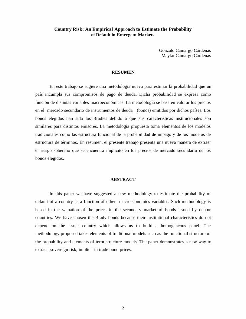
Country Risk: An Empirical Approach to Estimate the Probabilityof Default in Emergent Markets

Gonzalo Camargo CárdenasMayko Camargo Cárdenas

RESUMEN

En este trabajo se sugiere una metodología nueva para estimar la probabilidad que un

país incumpla sus compromisos de pago de deuda. Dicha probabilidad se expresa como

función de distintas variables macroeconómicas. La metodología se basa en valorar los precios

en el mercado secundario de instrumentos de deuda (bonos) emitidos por dichos países. Los

bonos elegidos han sido los Bradies debido a que sus características institucionales son

similares para distintos emisores. La metodología propuesta toma elementos de los modelos

tradicionales como las estructura funcional de la probabilidad de impago y de los modelos de

estructura de términos. En resumen, el presente trabajo presenta una nueva manera de extraer

el riesgo soberano que se encuentra implícito en los precios de mercado secundario de los

bonos elegidos.

ABSTRACT

In this paper we have suggested a new methodology to estimate the probability of

default of a country as a function of other macroeconomics variables. Such methodology is

based in the valuation of the prices in the secondary market of bonds issued by debtor

countries. We have chosen the Brady bonds because their institutional characteristics do not

depend on the issuer country which allows us to build a homogeneous panel. The

methodology proposed takes elements of traditional models such as the functional structure of

the probability and elements of term structure models. The paper demonstrates a new way to

extract sovereign risk, implicit in trade bond prices.

3

Country Risk: An Empirical Approach to Estimate the Probabilityof Default in Emergent Markets1

Gonzalo Camargo CárdenasMayko Camargo Cárdenas

The main purpose of this paper is to propose a new methodology that allows the

estimation of the probability of default of a country and to recognize the variables that

determine its evolution in time. The paper demonstrates a new way to extract sovereign

risk, implicit in trade bond prices.

In order to do so, we present the preliminary research on this field, some of which

will be empirically checked with the methodology suggested in this work. We have been

specially careful to stand out the significant variables used in determining the probability

of default of a country.

Most of papers in sovereign risk try to built a theoretical model to determine the

payment availability of a country and then evaluate it empirically (Kharas (1984), Taffler

and Abasi (1984) and Dym (1991); while other authors like Di Mauro and Massola

(1989), Evans and Cumby (1993), Favero and others (1996) try to determine empirically

the variables that explain the probability of default of a country. These works make

methodological suggestions on the estimation of the probability issue.

In Chart 1, we show the most relevant research on this field and the significant

variables that explains the probability of default

1 An earlier version of this paper was the thesis of CEMFI post graduate course of one of the

authors. We are very grateful to Manuel Arellano, Enrique Sentana, Samuel Bentolilla, MiguelSebastian, Manuel Balmaceda, Rafael Repullo and others by their helpful comments. Theopinions and conclusion are of the authors’ entire responsibility. Other previous version won thesecond place in the Research Contest for Young Economist 2000 that was organized by theCentral Reserve Bank of Peru. Any remaining mistakes is our own responsibility.

4

Chart 1. Country-Risk: Research and Conclusions

MODEL Explanatory Variable.*Frank and Cline (1971)Discriminant.

Debt service, debt amortization/external debt.

Feder y Just (1977)Logit

Debt serv. ; import./reserves; income per-capita; capitalinflow/debt service

Mayo y Barret (1978)Logit

External debt/exports; reserves/import.; imports /GDP;I.M.F Reserves/imports; inflation.

Feder, Just y Ross (1981)Logit

Debt service; GDP per-cap/GDP per-cap in EE.UU.;reserves/imports; exports/GDP; trade inflows/debt service

Taffler y Abasi (1984)Discriminante

External debt/exports; inflation; domestic capital/GDP.

Cline (1984)Logit

Debt service; import/reserv.; amortization/ext. debt; currentaccount deficit./export.; growth rate of income per-cap.;global credit abundance

Kharas (1984)Probit

Debt serv./GDP.; import./GDP.; debt/export.; serv.Debt/export.; GDP per cap.; GDP growth

Mc Fadden y otros (1985)Probit

Reserv./GDP.; import./GDP; debt/export.; serv.debt/export.; GDP. per-cap.; GDP growth

Di Mauro y Mazzola(1989)VAR

Export growth; GDP growth; public expense growth.; CPI;reserv./import; LIBOR.

*In this column we show the variables with significant coefficients that the differentauthors found in order to explain the probability of default of the countries.

In the following pages we introduce the methodology used for the estimation of the

probability of default and the variables that determine it. Afterwards we will use this

methodology to evaluate some of the models presented previously. Finally, we will show

the most important results of the estimations.

1. METHODOLOGY

The model proposed intends to estimate the probability of default as a function of

macroeconomic variables (economic fundamentals). To do so, we will build a valuation

model of bonds issued by developing countries. In this way we can use the information

contained in the prices of the secondary market of sovereign bonds. We will suppose that

the default probability (sovereign risk) is implicit in traded bond prices.

5

We have chosen the par and discount Brady bonds for the econometric estimation.

One of the reasons we have made this choice is the similar institutional characteristics

among the countries that have been able to issue this type of bonds. On the other hand,

these bonds are considered among the most liquid instruments of developing countries,

just like the “C” bonds of Brazil.

It is important to remember that the principal of Brady bonds is fully collateralized

by U.S. Treasury securities, which means that in case of default before the deadline, the

creditor will execute the complete collateral.

Another characteristic of this type of bonds (discount type) is the immediate

renewal of the collateral of the coupons 2(rolling interest collateral), which means that if

the debtor pays the coupon the collateral is automatically “rolled over” to protect the next

interest payments and so on until the bond maturity or default.

Being risky bonds, the market valuation of this instrument and its price depends on

the probability of default and other factors. Therefore, if we denote the price as a function

of the probability of default, we will be able to build a model for that probability.

The strategy to build that model has two steps. In the first one, we make a

valuation model of Brady bonds. As we previously state, the price of a bond is the present

value of the expected stream of cash flows arising from the interest collateral and the

coupon payments, discounted at an interest rate. Anyway, as the Brady bonds come from

countries with certain levels of risk, there is always the chance that the country decide not

to pay a specific coupon. On the other hand, in par and discount Brady bonds, the interest

payments and the principal are typically guaranteed with a collateral. All these

characteristics must be included in the valuation model of such bonds.

After the valuation of the Brady bonds, we get the bonds’ price as a function of the

probability of default of each coupon and the expected values of its guaranties. In this

second part of the analysis, we use a probability model that permits the expression of such

6

probability of default as a function of observable variables in each country. In this way,

the observed prices in the secondary market of the Brady bonds are related with

macroeconomic variables that reflects the economic performance of the countries.

At this point we are going to establish the notation we are using in this work.

Being the probability valuated at the moment t that the country i does not pay at any

instant between the present moment and the maturity of the coupon j, denoted by Prob ti (t,

t+j).

Let the implicit forward rate valued at time t from instant t+a to t+b be denoted by

f(t:a,b). The spot rate at time t, from time t to t+s will be denoted by r(t; t +s) or rt t s, + . for

abbreviating.

The coupon that the country i owes, calculated to the rates in force in t and that

must be paid at the moment j will be noted by Ct t ji, + and the principal in t that must be

paid at the maturity of the bonds, will be expressed as Pr .in ti

To build the risk-free rate yield curve we have used the U.S. Treasury’s coupon

zero curve. The sequence of interest rate applicable every week for different terms:

{r;(t;t+s)} where s=1 month, …30 years, is obtained at weekly frequencies from

Bloomberg3. The term structure for the necessary coupon dates is then constructed using

the method of Nelson-Siegel (1987)4.

The estimation of the coupon zero curve and the spot rates for each day of the

period considered allows us to compute the entire structure of forward rates. In t, with

discrete compounding, the structure of forward rates is:

2 The collateral of the interest in Brady bonds is the cash invested in bonds of the USA Treasury or

other approved instruments (with categories above AA)3 Bloomberg is the name of an electronic data base that offers financial information in real time. Is

one of the most used instruments in the market analysis because it provides information of almostevery aspect of a country.

4 For more information about the estimation of the term structure it is recommended to seeappendix 1.

7

(1) 1);(1);(1

),:( −++++

=attrbttr

batf

The structure of forward rates is necessary in order to compute the rolling interest

collateral (essential feature of discount Brady bonds); when a coupon is paid the collateral

automatically “rolls over” to protect the 12, 14, or 18 months of interest payments, all the

way up to maturity or default. Therefore, the value of the coupon collateral that dues at j

time, valued at that moment at interest rates applicable at E It t ji( )+ is obtained according

to:

(2) E IC

f t j j it t ji t j

i

i( )

( ( ; , ))++=

+ +∑ 1

where the summation is taken over the number of periods for which the interest payments

are collateralized.

It has been mentioned that the discount Brady bonds have floating coupons equal

to the Libor rate to six months plus a premium. To compute the expected coupons at t, the

paper relies on weekly data on the swap curve at maturities of 1,2 and 6 months, and 1, 2,

3, 4, 5, 7, 10, 17 , 20, and 30 years. This information was obtained from Bloomberg

(Izvorski, 1998). We have used the cubic spline interpolation to complete the swap

structure across the remaining dates and maturities (Izvosrki, 1998)

1.1 First Stage in the construction of the model: Valuation of the Brady Bonds

In order to explain the deduction of the valuation model, we are going to use the

intuition in a very simple case. Suppose that the country i has issued one bond with

maturity two periods from now and that at the end of each period pays one coupon. For

making it easier, lets assume that the payments of the coupons have Brady type’ collateral,

and that there is no principal to pay, meaning that the only risk that the creditors has is

referred to the payment of the interests. If there is a situation of no payment of the first

coupon, the creditors will execute the collateral and the process stops.

8

The payment structure of this type of instruments is as follows:

Payments at the end of t+1:

++

+

+

)1,(Pr w/p)(

)1,(Pr-1 w/p

1

1

ttobIE

ttobC

ttt

tt

The payments to the creditors at the end of the period t+2 if the debtor pays in t+1

are:

Payments at the end of t+2:

++++

+

+

)2,1(Pr w/p)(

)2,1(Pr-1 w/p

2

2

ttobIE

ttobC

ttt

tt .

Therefore, assuming a perfect market and risk neutrality, the present value of such

instrument should be:

(3)P

C ob E I obr

C ob ob E I ob obr

ti t t t

i t t t t ti t t

t t

t t ti t t t

i t t t t ti t t t

i t t

t t

=−

++

− − −+

+ + + + +

+

+ + + + + + + + +

+

, ( , ) ( , )

( ; )

, ( , ) ( , ) ( , ). ( , )

( ; )

( Pr ) ( ).Pr( )

( Pr )( Pr ). ( ).Pr ( Pr )( )

1 1 1 1

1

2 1 2 1 1 1 2 1

2 2

11

1 1 11

The same argument can be used to multi-period bonds with a principal different to

zero. So, if the present value of a bond is the present value of the expected stream of cash

flows arising from the interest collateral and the coupon payments discounted at the

riskless rate, it is proved under risk neutrality, that the price of a bond issued by the

country i at the instant t can be express in the following desegregated way:

(4)

NNtt

it

NNtt

NttitNtNti

tNttNttitNtt

NNtt

NttitNtNti

tNttNttitNtt

tt

ttittti

tttttittt

tt

ttittttti

tttit

rin

robobIEobC

robobIEobC

robobIEobC

robIEobC

P

)1(Pr

)1()Pr1(Pr).().Pr1(

)1()Pr1(Pr).().Pr1(

. . .)1(

)Pr1(Pr).().Pr1()1(

Pr).()Pr1(

),();(

)1,().,1(),(,

1))1(;(

))2(,()).1(),2((1))1(,(1,

2)2;(

)1,().2,1(2)2,(2,

)1;(

)1,(1)1,(1,

++

−++−+++++

−−+

−+−+−+−++−+−+

+

+++++++

+

+++++

+++

−−

++−−

+++−−

++−

=

9

Remember that the discount and par Brady bonds have a maturity of about 30

years and that they pay semi-annual coupons. So, the expression (4) can be written in a

compact way, as:

(5)

NNtt

it

N

jjjt

jtjtitjtti

ti

jttjttit

ijtti

t

rin

robobIEobC

P

)1(Pr

)1()(Pr)Pr1).(()Pr1(

);(

1 );(

),1(.))1(,(),(,

+

=

+−+−+++++

+

+∑ +−−

=

where

• 11( ),+ +rt t j

j discount factor in force in t for j periods to come

• Pr( )

:,

inr

i

t t NN1+ +

value in t of the principal which expires N periods to come

In the equation (5), as Evans and Cumby suggest (1993), we incorporate the

possibility that the market assign different default probabilities at t for the different

coupons of the same bond. However, many models that have tried to estimate the default

probability (Izvorski, 1998; Bierman and Hass 1975) suppose that:

(6) Pr Prob t t j ob t t jti

ti ( , + ( - )) = ( , + ); j 1 ∀

The papers that assume a constant probability of default for different periods

solve the valuation equation like (5), with a numeric algorithm just like the one of

Newton-Rapshon5.

In the estimation we will test the nule hypothesis: the default probabilities for dates

t>s viewed from date s are no constant. It is the way to evaluate if the suggested situation

of constant probabilities does verify or not.

5 For more information about non linear models we recommend Greene (1990), Amemiya (1983)

and Quandt (1983).

10

In order to get the model to be estimated we use the following proposition:

Proposition 1: Deduction of Default Probabilities: The equation (5) can be expressed as

(7)

PC

r

E I C

r

E I

rob t t j

inr

ti t t j

i

t t jj

j

N

t t ji

t t ji

t t jj

t t ji

t t jj

j

N

ti

ti

t t NN

=+

+

−

+

−

+

+

++

+

+=

+ +

+

+ +

+ ++

=

+

∑

∑

,

,

,

,

( )

, ( )

,

( )

( )

( )

( )

( ).Pr ( , ))

Pr( )

1

1 1

1

1

1

11

1

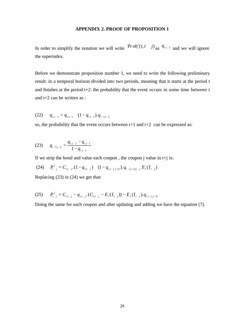
Proof: See appendix 2

If we change variables, the equation (7) can be written as

(8) P A F ob t t jti

ti

t t ji

ti

j

N

= + ++=

∑ , . Pr ( , )1

where:

• AC

rti t t j

i

t t jj

=+

+

+

,

,( )1

• FE I C

r

E I

rt t ji t t j

it t ji

t t jj

t t ji

t t jj,

,

,

( )

, ( )

( )

( )

( )

( )++ +

+

+ +

+ ++=

−

+

−

+

1 1

1

11

Finally, if we add an error term to the equation (8) we obtain the model to estimate

(9) P A F ob t t j eti

ti

t t ji

ti

ti

j

N

= + + ++=

∑ , .Pr ( , )1

being the error term a “white noise”6

6 This error term pretends to gather the stochastic perturbations on which the market prices of the

Brady bonds are attached. This contributes to explain the observed prices in the market.

11

1.2 Second Stage: A Model for Default Probabilities

After building an expression of the prices of the Brady bonds related to the

probabilities of default for different maturities, we will try to build a model for such

probabilities where we can introduce variables in equation (9) that reflects the economic

behavior of a country or economic fundamentals.

It is a well known practice in risk-country literature to assume that a country

announces a default at the moment t+j when a variable Z* (which represents the

availability or payment capacity) reaches a critical value K. That is why in order to

estimate the risk of default j in forward periods it is necessary an expression for

).(Pr **tjt

it ZKZob =+ But *

tZ is an unobservable variable. So, to express such probability

in observable variables ( ),X t it will be assumed that:

(10) )).((),(Pr.)(Pr * jtXFjttobXKZob it

ittjt

it ++′=+==+ δβ

where F(.) is the accumulated distribution function of the logistical distribution and δ is

the parameter that intends to take in the effect of the different maturities of the coupons

over the probability of default valuated in t.

In accordance to this, the equation (10) can be expressed as:

(11) Pr ( , )exp( . ( ))

exp( . ( ))ob t t j

X t jX t jt

i ti

ti+ =

′ + ++ ′ + +

β δβ δ1

Replacing (11) in (10) the valuation model to estimate will be:

(12)iti

t

iti

Nttit

iti

Ntt

it

iti

ttit

iti

ttit

it

eNtX

NtXF

NXNtX

F

tX

tXF

tX

tXFAP

+++′+

++′+

−+′+−++′

+

+++′+

++′+

++′+++′

+=

+−+

++

)).(exp(1)).(exp(

))1.(exp(1))1.(exp(

....

...))2.(exp(1

))2.(exp(

))1.(exp(1

))1.(exp(

,)1(,

2,1,

δβδβ

δβδβ

δβδβ

δβδβ

12

In a more compact way, (12) it can be written as follows:

(13) P A FX t j

X t jet

iti

t t ji

j

Nti

ti t

i= +′ + +

+ ′ + +++

=∑ , .

exp( . ( ))exp( . ( ))1 1

β δβ δ

where

• β is a vector of kx1 dimensions.

• X tiis the vector of explaining variables related to the country i.

It must be said that such vector of explaining variables is as follows:

[ ]X C D Z Wti i

ti

t= ,

C : constant expression (common for every country)

Di : vector of specific dummies for each country

Zti : vector of specific variables for each country that varies on time.

Wt : vector of common variables for every country that varies on time.

The selection of variables that are part of the vector X ti has been made with the

results of previous empirical researches and the available data of each variable for the

countries in the panel.

To simplify the notation, the model presented in (13) will be expressed as

(14) it

it

it ejtXhP +++′= )).(( δβ

The estimation of the data has been made with ordinary non linear least squares

and the econometric programs used has been TSP and Math Lab.

13

The enlargement of the theory of non linear models to the panel data estimation is

not difficult, the main difference in this case is that the individual specific effects cannot

be eliminated by taking first differences. It is going to be necessary to incorporate

dummies in order to capture these effects.

Afterwards we show the results with the Gauss-Newton’ estimation algorithm. The

results obtained with the Newton Rapshon algorithm were similar, which proves the

robustness of the model to the type of process used and the probable existence of one

unique global maximum.

The estimations have been made for two types of Brady bonds: par (which coupons

are fixed when the bonds are issued) and the discount bonds (that have coupons attached

to a floating rate which is generally the Libor rate plus a premium, in most cases this is

81.25 basic points). In every case, the results have been similar. All the Bradies used in the

estimation have been issued in the 90’s, with semi-annual coupons and expiration dates

after the year 2010.

We have used monthly data for the valuation and the period considered goes from

June 1996 to December 1998. We have chosen this period because it was the only one

with available data to build a balanced panel. The data frequency have been determined by

the availability of the macroeconomic series of the countries, which at best is a monthly

frequency.

We have daily information since 1990 about the countries that issued Brady bonds

at the start of the program, but there are plenty of peculiarities. For example: In a lot of

cases we can observe that the price stays the same during several months or even years.

This can be due to the fact that the bond did not quote prices during that period. It also

happens that the price data of a bond suddenly disappears in one moment until it shows

again, several months later.

These problems with quotations has been the main criteria to determine the sample

of countries, which finally includes Argentina, Brazil, Jordan, Nigeria, Russia, Ecuador,

Peru and Venezuela. With this sample we were able to build a balanced panel. All of these

14

countries have between 12, 14 or 18 months of guaranteed coupons on very liquid

instruments of the USA Treasury. The amounts issued varies considerably depending on

the issuer country and the type of instrument used7.

We have used the daily price list of the Brady bonds (discount and par bonds) that

appears in Bloomberg. We have used in the estimation -like it is common in this kind of

research (Izvorski (1998)-, the bid prices. The monthly data of prices was built taking the

weighted average of the daily quotations within a month. The reason we have used this

method instead of taking the quotation of the last day of the month is because we try to

avoid taking atypical values associated with the last quotation.

In order to obtain the macroeconomic series we have used several sources. The

information about Latin America countries comes from Latindat, a data base built by the

Economics Studies Office of the Bilbao Vizcaya Argentaria Bank that includes almost all

of the most important economic series of Latin America countries.

For the rest of the countries, the most used source has been the cd-rom of

International Statistics prepared by the International Monetary Fund (IMF-Stat). We have

also checked the bulletins and Internet websites of each Central Bank. The data on

external debt and its services come from the data base of the International Payment Bank

in Basilea (BIS). The data about the interest rates curves (spot, forward and swap) is from

Bloomberg.

The period considered for all the estimations goes from June, 1996 to December,

1998. The panel has nine countries which makes a total of 279 observations.

7 For more information about the characteristics of the Brady bonds we recommend Merril Lynch

(1995) or Bloomberg.

15

2. RESULTS OF THE ESTIMATIONS

As we say in the introduction of the paper, the main purpose of this paper is to

propose a new methodology that using the market information allows the estimation of

the probability of default of a country and to recognize the variables that determine its

evolution. The variables of the vector Xti have been chosen from the conclusions of other

models .

We will first show the results of the estimation for the Tafler & Abbassi (1984) and

Kharas (1984) models. After that we will show the estimations results of the Dym (1994)

model. This is the model with most success in predicting the value of the dependent

variable (market prices of Brady Bonds) and have the highest levels of overall and

individual significance.

We have used two different specifications for each model. The difference between

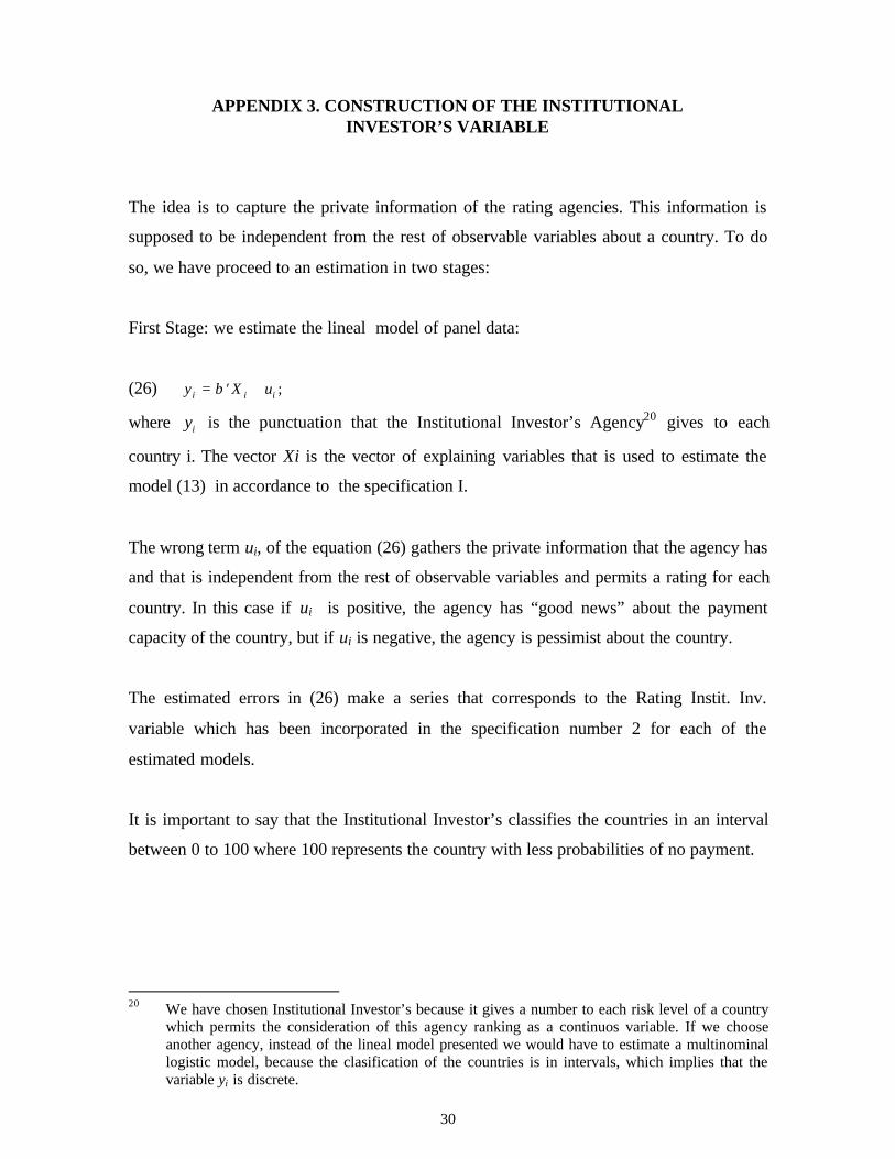
them is that one includes the Institutional Investor's Rating variable. With this variable we

try to get the private information that Ranking Agencies have about the payment capacity

of one specific country (the methodology that we have used to build this variable is shown

in the appendix 3).

All the results correspond to the Brady discount bonds estimation. The results of

the estimation for Par Bonds were similar. Before showing the results we must remember

that the first derivative of the default probability regarding a exogenous variable is:

(15)∂

∂β β β

Pr ( , ). ( ).( ( ))

ob t t jK

F X F Xt

kk t t

+= ′ − ′1

16

The sign of the estimated coefficients have the following interpretation:

(16) if

<⇒<

>⇒>

0),0(Pr

0

0),0(Pr

0

k

kk

Xjob

Xjob

∂∂

∂∂

β

So, if the associated coefficient of a exogenous variable has a positive sign, it

means that the increase of the level of this variable has positive effects in the default

probability and therefore it is an indicator that the external vulnerability of such economy

increases. The increment of default risk damages the perception of the market about the

debtor and therefore reduces the bond prices issued by the debtor.

Chart 2. Results of the estimation of Taffler and Abbasi (1984) Model8

Variables Specif. 1 Specif. 2Fin. Debt/Export 0.025

(0.05)1.001(0.07)

Inflation 0.108*(0.051)

0.077*(0.041)

Domest. Capital /GDP. -2.309**(0.093)

-1.579**(0.198)

Rating. Institutional Inv --- -1.661(0.978)

Constant Term -2.158**(0.236)

-2.663**(0.437)

∂ 0.1579**(0.0373)

0.1623**(0.0497)

-2*Ln. obs

101.54279

105.98279

** Significant at 99%. *Significant at 95%. In othercases no significantL: log of likelihood function

We have not shown in chart 2 the coefficients that corresponds to the variables

with specific effect of each country (country dummies). It must be said that all of them are

positive and significant for a confidence level of 99%.

8 The standard errors are robust to heteroskedasticity and first order autocorrelation.

17

The goodness of fit for the Taffler and Abassi model is due to the constant term,

the specific effects of each country and the ratio domestic capital/GDP. The reason why

the ratio Financ. Debt/export has not significance, can be due to the fact that both

variables are not completely independent, but present significant correlation within each

country.

The comparison with the results of the original model is not possible in this case

because we have chosen a different country sample for each different period.

The parameter “∂“ is significant and has a positive sign, which means that the

market punishes longer maturities terms. The presence of this variable can contribute to

the better adjust of the model because it allows to make a polynomial of exponential

functions with order equal to the logest maturity.

Chart 3. Results of the estimation of Kharas Model (1984) 9

Variable Specif. 1 Specif 2.Debt Serv./GDP 0.026*

(0.014)0.081*(0.042)

Import./GDP 0.066(0.041)

0.072(1.284)

GDO. Per cápita -0.0072(0.014)

-0.015(0.012)

GDP Growth -0.0083*(0.041)

-0.0041*(0.002)

Rating. Institutional Inv ---- -0.0134**(0.0014)

Constante -2.370**(0.072)

-2.572**(0.077)

∂ 0.125**(0.035)

0.189**(0.042)

-2*Ln. obs

256.32279

289.65279

** Significant at 99%. *Significant at 95%. In othercases no significantL: log of likelihood function

9 The standard errors are robust to heteroskedasticity and first order autocorrelation.

18

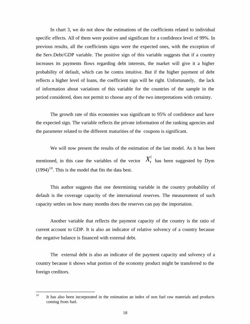
In chart 3, we do not show the estimations of the coefficients related to individual

specific effects. All of them were positive and significant for a confidence level of 99%. In

previous results, all the coefficients signs were the expected ones, with the exception of

the Serv.Debt/GDP variable. The positive sign of this variable suggests that if a country

increases its payments flows regarding debt interests, the market will give it a higher

probability of default, which can be contra intuitive. But if the higher payment of debt

reflects a higher level of loans, the coefficient sign will be right. Unfortunately, the lack

of information about variations of this variable for the countries of the sample in the

period considered, does not permit to choose any of the two interpretations with certainty.

The growth rate of this economies was significant to 95% of confidence and have

the expected sign. The variable reflects the private information of the ranking agencies and

the parameter related to the different maturities of the coupons is significant.

We will now present the results of the estimation of the last model. As it has been

mentioned, in this case the variables of the vector Xti has been suggested by Dym

(1994)10. This is the model that fits the data best.

This author suggests that one determining variable in the country probability of

default is the coverage capacity of the international reserves. The measurement of such

capacity settles on how many months does the reserves can pay the importation.

Another variable that reflects the payment capacity of the country is the ratio of

current account to GDP. It is also an indicator of relative solvency of a country because

the negative balance is financed with external debt.

The external debt is also an indicator of the payment capacity and solvency of a

country because it shows what portion of the economy product might be transferred to the

foreign creditors.

10 It has also been incorporated in the estimation an index of non fuel raw materials and products

coming from fuel.

19

Another solvency indicator is the portion of the GDP that is public deficit or

surplus because the negative balances will turn into more debts.

The inflation rate is usually used as an indicator of long term perspectives and the

stability of an economy.

In order to evaluate the effects of the higher global credit availability on the

market perception of the payment capacity of a country, we have considered the rate of

growth of the world GDP.

The graphs of the probability of default in a four-year-term for each country, after

using the Dym model (1994) under specification 2, can be seen in the appendix 6.

The coefficients’ signs in the reserves/importation variables and growth of the

world GDP11, indicates that the increment in these variables reduces the probability of

default. This result coincides with the theory. The opposite happens with the coefficient

of the financial debt/GDP variable. The negative value of this variable indicates that the

more debts a country have, the risk of no payment decreases. But this variable is not

significant in either of the two specifications (maybe the addition of debt stock with

international organisms and governments may increase its significance).

11 The presence of this variable intends to show the presence of the “flight to quality”

phenomenom.

20

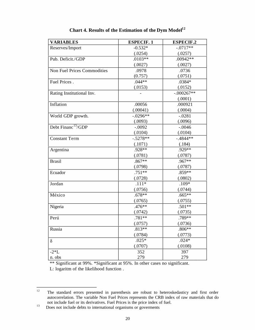
Chart 4. Results of the Estimation of the Dym Model12

VARIABLES ESPECIF. 1 ESPECIF.2Reserves/Import -0.532*

(.0254)-.0717**(.0257)

Pub. Deficit./GDP .0103**(.0027)

.00942**(.0027)

Non Fuel Prices Commodities .0978(0.757)

.0736(.0751)

Fuel Prices . .044**(.0153)

.0384*(.0152)

Rating Institutional Inv. - -.000267**(.0001)

Inflation .00056(.00041)

.000921(.0004)

World GDP growth. -.0296**(.0093)

-.0281(.0096)

Debt Financ13/GDP -.0092(.0104)

-.0046(.0104)

Constant Term -.5278**(.1071)

-.4844**(.184)

Argentina .928**(.0781)

.929**(.0787)

Brasil .867**(.0798)

.967**(.0787)

Ecuador .751**(.0728)

.859**(.0802)

Jordan .111*(.0756)

.109*(.0744)

México .678**(.0765)

.665**(.0755)

Nigeria .476**(.0742)

.501**(.0735)

Perú .781**(.0757)

.789**(.0736)

Russia .813**(.0784)

.806**(.0773)

δ .025*(.0707)

.024*(.0108)

-2*Ln. obs

352279

397279

** Significant at 99%. *Significant at 95%. In other cases no significant.L: logaritm of the likelihood function .

12 The standard errors presented in parenthesis are robust to heteroskedasticy and first order

autocorrelation. The variable Non Fuel Prices represents the CRB index of raw materials that donot include fuel or its derivatives. Fuel Prices is the price index of fuel.

13 Does not include debts to international organisms or goverments

21

The Institutional Rating Inv variable, has also a negative estimated coefficient,

which means that the “good-news” of an agency regarding a country, reduces its

probability of no payment (this explanation is valid because a higher punctuation in the

agency’s ranking means less chances of no payment). So, we can say that the Institutional

Agency Investors’ opinion contributes to make a market evaluation about the payment

capacity of a country.

The coefficient of the inflation and public deficit/GDP variables is significant and

positive, which means that if any of the variables values increases the same will occur

with the estimated probability default. This result is consistent with the relation between

these variables and the risk of a country.

The value of the coefficient of fuel prices is positive, maybe because we have

included in the sample exporter and importer countries nets of fuel. In order to separate

this two kind of countries, we multiply these variables by a dummy that takes the numeric

value of one when we dealt with an exporter country of fuel. Unfortunately, this variable

did not allowed the model convergence.

The price index of raw materials other than fuel has a positive value, but has a

insignificant coefficient. In this chart, we do not present the valuation of the coefficient

related to current account because it has no significance in any of the cases.

It is important to say that the parameter δ is significant and takes positive values

which means that the probability of no payment varies proportionally with the maturity of

the bond. This is the evidence against the assumption of keeping constant the probability

of default for different maturities. This conclusion coincides with the results of Evans and

Cumby (1993).

The dummies that gather the unobservable heterogeneity of each country are all

significant on the 95% of confidence.

As seen in chart 4 we have included in addition to the variables proposed on the

model by Dym (1991), the prices of fuel and other commodities different from fuel. Even

22

when these variables may me related to the inflation on each of the counties of the chart,

their inclusion will only affect the steadiness of the estimated parameters (Green, 1990).

In order to evaluate if the specification of this model is correct, in other words if

the dummy variables that collects the specific effects of each country must be included in

the equation, we have used the Wald’s specification test for non linear models, getting the

following results:

Non restricted: ;)).(( it

it

it ejtXhP +++′= δβ where: X t

i = [ C Di Zti Wt ]

and

Restricted Model: ;)).(( it

it

it ejtXhP +++′= δβ where: X t

i = [ C Zti Wt ]

The Wald´s statistic is obtained valuating the model without the restrictions on the

coefficients (unrestricted model) that specify the nule hypothesis.

(17) Ho(1) :β Di = 0

where

β Di : are the coefficients related to each dummie of the vector .iD

This test evaluates if the coefficients of the unrestricted estimation satisfy the

restrictions that specify the nule hypothesis.14

14 The Wald’s statistics for models of the type . ,)( eXhy +′= β where β is a kx1 vector of

estimated parameters, and restrictions of the type . H go : ( )β = 0 where g is a vector qx1 of

restrictions over β , can be expressed as W ng bg

Vg

g b= ′ −( ) (( ) ( )

) ( )∂ β

∂β∂ β

∂β1 where n is the

number of observations, b is the vector of estimated parameters under the no restricted model

and V is the covariance’s matrix estimated of b, that is obtained from V nS h h= −2 1( ) ,∂∂β

∂∂β

where S u un k

2 = ′−

being u the vector of residuals from the non restricted model.

23

Formally, under the nule hypothesis, the asymptotic distribution of the Wald’s

statistic is a χ2(q) where q is the number of restrictions of Ho.

With the same purpose we have used the test of likelihood ratio.15

In both cases the nule hypothesis is rejected. So, it can be said that the model

presented in chart 4 must include the dummy variables that gathers the specific effects of

the countries.

In spite of its versatility one of the disadvantages of this type of models is the lack

of steadiness. To evaluate if the estimators obtained in the model (13) come from the same

population independently of the sample size, the total period has been divided into two sub

samples and it is contrasted the following nule hypothesis:

(18) Ho I II( ):2 0β β− =

where the unrestricted model is:

(19)

+++′=+++′=

II sample sub for the ;)).((

I sample sub for the ;)).((it

itII

it

it

itI

it

ejtXhP

ejtXhP

δβδβ

and the restricted model is:

(20) sample entire for the ;)).(( it

it

it ejtXhP +++′= δβ

The first sub sample goes from June 1996 to august 1997 and the second sub

sample goes from September 1997 to December 1998. In this way we have two identical

periods.

15 For the sample of n observations, assuming that the errors are normally distributed, the likelihood

ratio is: RV L L= −2(ln ln *), where L* is the value taken by the likelihood function under the

restricted model. The statistic RV is distributed as a χ2(q), being q the number of restrictions.

24

In order to evaluate the nule hypothesis (Ho(2)) for each of the specifications of

the model (13) presented in chart 4, it has been used the test of the likelihood ratio. The

results of this test are:

Chart 5. Results of the Parameters Stability Test

q LR Statistic. Critical Value (95% conf.)Specification 1 16 35.98 26.3Specification 2 17 39.16 27.6

As observed in chart 5, the nule hypothesis (Ho(2)) of overall equality of the

coefficients estimated on both sub samples is rejected at 95% . So, the estimations of this

model are not firm to the size of the sample16. This conclusion however is non unexpected

because the model is very complex and so it is very sensitive to the data and variables of

the estimation.

To explain the results, in chart 6 we show how the probability of no payment

estimated in December 1998 to a horizon of four years, varies if the explicative variables

increases 25%.

Chart 6. Country Rankings and Sensitivity of the Estimated Probabilities.

Countries17 Res/Imp PubDef/GDP Inflat %Risk./Jord*Russia -0.10 0.41 0.49 1.021Nigeria -0.60 0.09 0.07 0.665Venezuela -0.30 0.003 0.17 0.659Ecuador -0.16 -0.0218 0.25 0.459Brasil -0.42 0.09 0.01 0.376México -0.02 -0.002 0.11 0.361Perú -0.52 0.26 0.03 0.193Argentina -0.51 0.42 0.004 0.156Jordan -0.563 -0.01 0.003 -*Reference to the higher probability of default (n %) of the country compared to theone of Jordan.

16 Even though the suggested hyphotesis is rejected, the estimated coefficients for each sample,

coincide in sign and significance with the estimations of the restricted model.17 Ordenados de país con probabilidad de moratoria más alta hacia país con menor probabilidad de

moratoria. Las cifras del cuadro están en términos porcentuales.18 El dato negativo se refiere al efecto sobre la probabilidad de un incremento de 25% en el superávit

fiscal.

25

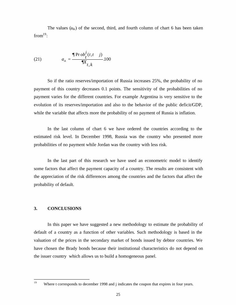
The values (aik) of the second, third, and fourth column of chart 6 has been taken

from19:

(21) aobt

i t t j

Xt kik =

+∂

∂

Pr ( , )

,.100

So if the ratio reserves/importation of Russia increases 25%, the probability of no

payment of this country decreases 0.1 points. The sensitivity of the probabilities of no

payment varies for the different countries. For example Argentina is very sensitive to the

evolution of its reserves/importation and also to the behavior of the public deficit/GDP,

while the variable that affects more the probability of no payment of Russia is inflation.

In the last column of chart 6 we have ordered the countries according to the

estimated risk level. In December 1998, Russia was the country who presented more

probabilities of no payment while Jordan was the country with less risk.

In the last part of this research we have used an econometric model to identify

some factors that affect the payment capacity of a country. The results are consistent with

the appreciation of the risk differences among the countries and the factors that affect the

probability of default.

3. CONCLUSIONS

In this paper we have suggested a new methodology to estimate the probability of

default of a country as a function of other variables. Such methodology is based in the

valuation of the prices in the secondary market of bonds issued by debtor countries. We

have chosen the Brady bonds because their institutional characteristics do not depend on

the issuer country which allows us to build a homogeneous panel.

19 Where t corresponds to december 1998 and j indicates the coupon that expires in four years.

26

The methodology proposed takes elements of traditional models such as the

functional structure of the probability and elements of term structure models, because it

uses the theory of rate expectations and the curves coupon zero.

Traditional logit and probit models explain the probability of default only if an

issuer has announced a default in the past at least one time. The difference of the model

suggested in this paper is that the methodology used allows the valuation of the

probabilities of default even when such fact has not been observed ever in the past. The

only requirement is that a secondary market of the instruments to valuate exists.

The logit and probit models cannot distinguish risk levels for different moments in

time. However, the method suggested allows the comparison of probabilities of default

estimated at the present time for different maturities. It also makes it possible to build a

structure curve of probabilities for different maturities and to make a continuos ranking of

probabilities.

The methodology used in this document related to the discriminate analysis models

has the advantage to enable the addition of qualitative variables that reflects aspects such

as the reputation or social/political situation of the country in the valuation of the

probabilities of default.

The suppositions on which the valuation is based are the same required in term

structure models. However in this case it has not been necessary to discompose the

spreads in order to find a value for the probability of default and then, in a second stage set

up a model that explains such probability. Instead, the estimated coefficients have been

directly obtained from the information included in the market prices.

From the empiric exercises made we can observe that some variables that were

important in other research to explain the probability of default, are no more important

when they are contrasted with the methodology used in this paper. However, the

comparison with such works is not possible because the periods considered and the

number of countries are different.

27

From the models evaluated, the one that fits the data best is the Dym model (1994).

In this case the significant variables directly related with the payment capacity of a

country are the public deficit and the inflation. The fuel price is also significant and affects

directly the probability of default. However, in this case the conclusions are not so clear as

in the previous variables because in the sample we have mixed the countries that import

and export fuel.

Among the variables which increment reduces the probability of default of a

country, we can find the reserves on importation and the growth of the world GDP. In the

other hand, if the private information of the Institutional Investor’s agency is positive

about the economy (“good news”), then the estimated probability of default must be

reduced.

Also important in the determination of the probabilities of default of a country are

the specific characteristics of the country. These variables were significant in all cases.

In the other hand, being the parameter ∂ significant, the model rejects the

hypothesis that the probability of default valuated at t can be constant for different

horizons.

One of the problems with this methodology is that because of its complexity the

model is not robust to the sample size and the number of variables chosen. However, in

the exercises the signs and significance of the estimated coefficients mostly do not change.

In this work we have intended to apply a new methodology to estimate the

probability of default of a country and to understand the way in which the evolution of

some of its macroeconomical variables determine its payment capacity, and therefore the

risk levels that the market gives to such country. The target has been to enrich the debate

about a standard way to evaluate the country risk.

28

APPENDIX 1. CONSTRUCTION OF THE TERM STRUCTURE CURVE

The information available about the structure of the interest rates of the USA Treasury

goes from June 1, 1996 to December 31, 1998. We got daily data for maturities of 30, 60

and 90 days and for maturities of 1, 2, 3, 5, 10, 12 and 30 years.

In order to build a structure of rates for all the terms it has been used the methodology

suggested by Nelson and Siegel (1987). In accordance to this the parameter vector to

estimate is: β β β β τ= ( , , , )0 1 2 1

The “forward” interest rate instantaneous for the term τ can be written as:

f 0 0 11

21 1

( , ) exp expτ β β βττ

βττ

ττ

= + −

+ −

The rate spot (yield of the coupon zero bond) is:

r( , ) ( ) exp expτ β β β βττ

ττ

βττ

= + + − −

− −

0 1 2

1

12

1

1

The parameter vector β , has been calculated daily. The estimation has been made using

non lineal least squares. For more information about the estimation of curves rates it is

recommended to see the works of Soledad Nuñez (1995) and Bobadilla (1999).

29

APPENDIX 2. PROOF OF PROPOSITION 1

In order to simplify the notation we will write Pr ( , )ob t t jti + as q t t, +1 and we will ignore

the superindex.

Before we demonstrate proposition number 1, we need to write the following preliminary

result: in a temporal horizon divided into two periods, meaning that it starts at the period t

and finishes at the period t+2. the probability that the event occurs in some time between t

and t+2 can be written as :

(22) q q q qt t t t t t t t, , , ,( ).+ + + + += + −2 1 1 1 21

so, the probability that the event occurs between t+1 and t+2 can be expressed as:

(23) qq q

qt tt t t t

t t+ +

+ +

+

=−

−1 22 1

11,, ,

,

If we strip the bond and value each coupon , the coupon j value in t+j is:

(24) P C q q q E It jj

t t j t t j t t j t j t j t t j+ + + + − + − + += − + −, , , ( ) ( ), ..( ) ( ). ( )1 1 1 1

Replacing (23) in (24) we get that:

(25) P C q C E I E I qt jj

t t j t t j t t j t t j t t j t t j+ + + + + + + −= − − −, , , , ( ).( ( )) ( ). 1

Doing the same for each coupon and after updating and adding we have the equation (7).

30

APPENDIX 3. CONSTRUCTION OF THE INSTITUTIONALINVESTOR’S VARIABLE

The idea is to capture the private information of the rating agencies. This information is

supposed to be independent from the rest of observable variables about a country. To do

so, we have proceed to an estimation in two stages:

First Stage: we estimate the lineal model of panel data:

(26) ;iii uXy +′= β

where yi is the punctuation that the Institutional Investor’s Agency20 gives to each

country i. The vector Xi is the vector of explaining variables that is used to estimate the

model (13) in accordance to the specification I.

The wrong term ui, of the equation (26) gathers the private information that the agency has

and that is independent from the rest of observable variables and permits a rating for each

country. In this case if ui is positive, the agency has “good news” about the payment

capacity of the country, but if ui is negative, the agency is pessimist about the country.

The estimated errors in (26) make a series that corresponds to the Rating Instit. Inv.

variable which has been incorporated in the specification number 2 for each of the

estimated models.

It is important to say that the Institutional Investor’s classifies the countries in an interval

between 0 to 100 where 100 represents the country with less probabilities of no payment.

20 We have chosen Institutional Investor’s because it gives a number to each risk level of a country

which permits the consideration of this agency ranking as a continuos variable. If we chooseanother agency, instead of the lineal model presented we would have to estimate a multinominallogistic model, because the clasification of the countries is in intervals, which implies that thevariable yi is discrete.

31

APPENDIX 4. ESTIMATED PROBABILITIES OF DEFAULT

The graphs of estimated default probabilities for a maturity of four years are shown in the

next pages.

Brazil

0 .00

0 .02

0 .04

0 .06

0 .08

0 .10

0 .12

0 .14

j u n - 9 6 a g o - 9 6 o c t - 9 6 d i c - 9 6 f e b - 9 7 a b r - 9 7 j u n - 9 7 a g o - 9 7 o c t - 9 7 d i c - 9 7 f e b - 9 8 a b r - 9 8 j u n - 9 8 a g o - 9 8 o c t - 9 8 d i c - 9 8

Ecuador

0 . 0 0

0 . 0 5

0 . 1 0

0 . 1 5

0 . 2 0

0 . 2 5


32

Jordan

0 . 0 0

0 . 0 2

0 . 0 4

0 . 0 6

0 . 0 8

0 . 1 0

0 . 1 2


Mexico

0 .00

0 .02

0 .04

0 .06

0 .08

0 .10

0 .12

0 .14


33

Niger

0 . 0 0

0 . 0 5

0 . 1 0

0 . 1 5

0 . 2 0

0 . 2 5


Peru

0 . 0 0

0 . 0 1

0 . 0 2

0 . 0 3

0 . 0 4

0 . 0 5

0 . 0 6

0 . 0 7

0 . 0 8

0 . 0 9


34

Russia

0 . 0 0

0 . 0 5

0 . 1 0

0 . 1 5

0 . 2 0

0 . 2 5


Venezuela

0 . 0 0

0 . 0 5

0 . 1 0

0 . 1 5

0 . 2 0

0 . 2 5

0 . 3 0


35

APPENDIX 5: CHARACTERISTICS OF BRADY BONDS USED IN THEESTIMATION

Chart 7: Summary of Discount Bradies

Country: Emission Date Emission amount/1 Day Month ReductionArgentina 31-Mar-93 4.300 15 4 0.35

Brazil 15-Abr-94 7.300 15 4 0.35Ecuador 28-Feb-95 1.435 15 4 0.45Jordan 24-May-94 0.157 30 3 0.45Mexico 28-Mar-90 11.764 30 3 0.35Niger 15-Abr-95 2.569 15 4 0.30Peru 16-Jun-95 1.365 30 3 0.35

Russia 22-Feb-95 3.265 15 3 0.30Venezuela 31-Mar-90 1.226 18 4 0.30

1/US$ billion dollarsDay: Number of day within the month, when the first coupon must bepaid.Month: number of the month of the maturity of the first coupon in the year. The nextcoupon maturity is six months laterReduction: It means the reduction over the originaldebtSource: Merril Lynch (1995), Bloomberg.

36

REFERENCES

Altman E.1989 “Measuring Corporate Bond Mortality and Performance”. Journal of Finance,

No. 44.

Amemiya T.1985 Advanced Econometrics. Cambridge, Mass. Harvard University Press.

Bierman, H. y Hass H.1975 “An Analytic Method of Bond Risk Differentials.” Journal of Financial and

Quantitative Analysis. December, 757-773.

Black, F. y Cox, J.C1976 “Valuing Corporate Securities: Some Effects of Bond Identidure Provisions”,

Journal of Finance, 31, 351-367.

Black, F. y Scholes, M.J1973 “The Pricing of Options and Corporate Liabilities”, Journal of Political

Economy, 81, No. 3, 637-654.

Bobadilla, G.1999 “Choosing the Right Error in Term Structure Models”. Tesina del CEMFI, No.

9904. CEMFI.

Cohen, D.1993 “A Valuation Formula for LCD Debt”, Journal of International Economics, 34,

167-180p.

Cohen, H., Kehoe, T.1998 “Self-Fulfilling Debt Crises”. Federal Reserve Bank of Minneapolis. Research

Department Staff Report 211.

Corcuera S. y García, J.C.1998 “El uso de las Mixturas de Distribuciones Gaussianas en Finanzas: Aplicación

en la Medición de Riesgo de Mercado y en la Valoración de Cobertura deOpciones Financieras”. Argentaria.

Cox, J. y Ross, S.1976 “The Valuation of Options for Alternative Stochastic Processes”, Journal of

Financial Economics, No. 3, 145-166.

Creditanstalt1997 The CA Country Model. Creditanstalt Economics Department.

Das, Sanjiv R.1998 Poisson-Gaussian Processes and the Bond Markets, National Bureau of

Economic Research. NBER Working Paper No. 6631.

37

Di Mauro, F. y Massola, F.1989 LDC´s Repayment Probems: A Probit Analysis. Temi di Discussione No. 116.

Banc di Italia, Roma. Mayo.

Duffie Gregory.1995 Estimating the Price of Default Risk. Federal Reserve Board. Washington,

September.

Dym, S.1994 “Identifying and Measuring the Risk of Developing Country Bonds”. The

Journal of Portfolio Management. Winter, 1994.

Evans, M. y Cumby, R1993 “Measuring Current and Anticipated Future Credit Quality: Estimate from

Brady Bonds”. New York University Salomon Center. Leonard N. SternSchool of Business. Working Paper Series S-93-94.

Favero, C., Giavazzi, F., Spaventa L.1996 “High Yields: The Spread on German Interest Rates”. Centre for Economic

Policy and Research (CEPR), Discussion Paper Serie No.1330.

Feder,G. y Just R.1977 A Study of Debt Servicing Capacity Applying Logit Analysis, Journal of

Development Economics 4, No. 1

Feder,G., Just R. y Ross, K.1981 Projecting Debt Service Capacity of Developing Countries. Journal of

Financial and Quantitative Analysis.

Fons, J.1994 “Using Defaults Rates to Model the Term Structure of Credit Risk”. Financial

and Analysts Journal, Setiembre-Octubre. pp. 25-32

Frank, C.R y Cline, W.R.1971 Measurement of Debt-Servicing Capacity: An Application of Discriminant

Analysis; Journal of International Economics. Vol 15.

Friedman, A.1975 “Stochastic Differential Equations and Applications” Vol 1, Academic Press,

New York.

Greene, W.1990 Econometric Analysis. 2da. ed. Macmillan Publishing Company. New York.

Hall, B.1996 Time Series Processor Version 4.3. User´s Manual.

38

Hamilton J.1991 “A Quasi-Bayesian Approach to Estimating Parameters for Mixture of Normal

Distributions”. Journal of Business Economic and Statistics. Vol 9, No. 1, 27-39.

Hernandez-Trillo, Fausto.1995 A Model Based Estimation of the Probability of Default in Sovereign Credit

Markets. Journal of Development Economics. Vol 4. 163-179.

Izvorski, Y1998 “Brady Bonds and Default Probabilities”. International Monetary Fund.

Research Department. WP/98/16

Kharas, Homi1984 “The Long Run Credit Worthiness of Developing Countries: Theory and

Practice”. Quarterly Journal of Economics. Vol. XCIX, No.3, 1984.

Keeming P.1994 Country Risk Analysis: Pre-Course Reading. CCF: 9th Inter Alpha Banking

School, 29 September.

Literman R. Y Iben T.1989 “Corporate Bond Valuation and the Term Structure of Credit Spreads”.

Journal of Portfolio Management. Pp 52-64.

Longstaff F., Schwartz E.1995 “A Simple Approach to Valuing Risky Fixed and Floating Rate Debt”. The

Journal of Finance. Vol. L, No.3. July, 1995.

Mayo, C. y Barret, F.1978 Country Risk: An Empirical Investigation. Journal of International Banking

and Finance.

Mc Fadden, D.; Eckaus,R; Feder, G; Hajivassilou, V. y O´Connell, S.1985 Is There a Life After Debt? An Econometric Analysis of the Credit Worthiness

Of Developing Countries. En: Smith, W y Cuddington, J. eds. InternationalDebt and the Developing Countries. (The World Bank Washington).

Merton R.C1975 “Option Pricing When Underlying Stock Returns Are Discontinous”. M.I.T.

Working Paper No. 787-75. (M.I.T., Cambridge, Mass).

Merril Lynch1995 “The 1995 Guide to Brady Bonds”. New York, N.Y.

Moody´s Investor Service1995 Sovereign Risk: Bank and Deposits vs. Bonds. October, New York.

39

Muñoz Rafael.1988 “Spreads y Gasto Fiscal: Una Aplicación a la Unión Europea”. Tesina -

CEMFI.

Nelson, C.R. and Siegel, A.F.1987 “Parsimonious Modelling of Yield Curves”. Journal of Business, 60, 473-489.

Núñez, S.1995 “Estimación de la Estructura Temporal de los Tipos de Interés en España:

Elección Entre Métodos Alternativos”. Working Paper, No. 9522, Banco deEspaña.

Pettis, Michael.1994 “Debt to Exports Ratios and Default Probabilities: The Implied Put Option On

Cashflows”. Columbia Journal of World Business. Summer 1994. Vol. 29.No.2.

Quandt, R.1983 “Computational Problems and Methods”. En Z. Griliches y M. Intriligator, eds.

Handbook of Econometrics. Amsterdam, North-Holland.

Saunders Anthony1997 Financial Institutions Management: A Modern Perspective. Irwin McGraw-

Hill,

Taffler R. y Abbasi M.1984 “Default and Renegotiations: An Approach to LDCs Debt”. Journal of

Quantitatives Methods, Vol. 2. No. 21

Vasicek O.1977 “An Equilibrium Characterization of the Term Structure”, Journal of Financial

Economics, 5, 177-188.

Wynn, R1989 Sovereign-Risk Quantification Methodologies: A Critique. En: Growth and

External Debt Management. Editado por H.W. Singer, Sharma Soumitra. MacMillan Press, 1989. Hong Kong.

country risk: an empirical approach to estimate the

Documents