countercyclical prudential tools in an estimated dsge model · we find that dp seems to outperform...
TRANSCRIPT

Prêmio Banco Central de Economia e Finanças
Jorge Luis Ponce MorenoCarlos Eduardo Serafín Frache DerregibusJavier García-Cicco
[email protected]@[email protected]
Brasília • 2016
Countercyclical prudential tools in an estimated DSGE model
Estabilidade Financeira • 3º lugar
Countercyclical prudential tools in an estimatedDSGE model∗
Serafín Frache1, Javier García-Cicco2 and Jorge Ponce †1
1Banco Central del Uruguay and dECON-UdelaR2Banco Central de Chile and Universidad Católica Argentina
August 7, 2017
Abstract
We develop a DSGE model for a small, open economy with a bank-ing sector and endogenous default. The model is used to perform a re-alistic assessment of two macroprudential tools: countercyclical capitalbuffers (CCB) and dynamic provisions (DP). The model is estimatedwith data for Uruguay, where dynamic provisioning is in place sinceearly 2000s. In general, while both tools force banks to build buffers,we find that DP seems to outperform the CCB in terms of smooth-ing the cycle. We also find that the source of the shock affecting thefinancial system matters to discuss the relative performance of bothtools. In particular, given a positive external shock the ratio of creditto GDP decreases, which discourages its use as an indicator variableto activate countercyclical regulation.
JEL classification numbers: G21, G28.Keywords: Banking regulation, minimum capital requirement, counter-
cyclical capital buffer, reserve requirement, (countercyclical or dynamic) loanloss provision, endogenous default, Basel III, DSGE, Uruguay.
∗The views in this paper are those of the authors and not necessarily of the institutionsto which they are affiliated.†Corresponding author: [email protected]
1
1 Introduction
In the wake of the global financial crisis of 2008-2009 it has become clear theimportance of systemic risk and the need for a macroprudential perspectiveto financial regulation. In this spirit, new prudential regulation has been es-tablished, being of particular importance Basel III, which strengthens bankcapital and liquidity requirements. Among other things, Basel III increasesminimum capital requirements, introduce more stringent liquidity regula-tion and introduces a counter-cyclical capital buffer. This last measure isintended to build capital buffers in booms, which may be used to (partially)absorb loses during a downturn, hence prudentially attending the cyclicaland endogenous raise in systemic risk during upturns. The implementationand efficiency of these regulations has been a topic of vivid debate amongpolicymakers and academics.
Regarding the implementation of countercyclical capital buffers, the de-bate is particularly relevant in jurisdictions where other macroprudentialinstruments developed to mitigate the prociclicallity of the financial sys-tem are currently in place. For example, Spain and several Latin Americancountries have been using dynamic loan loss provisions as a countercyclicalregulatory rule for several years.1 Under dynamic provisioning a fund is ac-cumulated in periods where the expected losses are lower than the long-run,or through-the-cycle, level. Dynamic provisions are not released in periodswith low default rates, but they are used to cover losses in a downturn.2
The aim of this paper is to perform a realistic assessment of the coun-tercylical regulation promulgated in Basel III, and to compare its relativeperformance with other macroprudential policies already used in many coun-tries, i.e. dynamic loan loss provisions. To do so, we develop a DSGE modelfor a small and open economy. Borrowers (called entrepreneurs) are modeledas in Bernanke et al. (1999), and can default on their loans. Banks use de-posits and own capital to lend to entrepreneurs and also to buy governmentbonds. Additionally, the banking sector is subject to prudential regulation.
1Recently, Spain stops using dynamic loan loss provisions in order to implement acountercyclical capital buffer.
2For the case of Spain, Jiménez et al. (Forth.) find that dynamic provisioning smoothscredit supply cycles and, in bad times, supports firm performance. In a formal model,Gómez and Ponce (2015) study the effectiveness of countercyclical capital buffers anddynamic provisioning to provide the correct incentives to bank managers and concludethat both of them are adequate policy tools.
2

The model is estimated with data for Uruguay, a country that has beenrunning a dynamic provisioning system since 2001. Finally, we perform sim-ulations of the key macroeconomic variables and of the banking sector underdifferent regulations in order to compare the results. More precisely, we com-pare the dynamics of this modeled economy with financial frictions when itis affected by external and domestic shocks under alternative macropruden-tial regulations: countercyclical capital buffers with alternative indicators ofthe financial cycle (i.e. GDP and credit) and different rules for loan lossprovisioning (i.e. static and dynamic).
We model the banking sector to account for different regulatory poli-cies and commonly observed facts in banking. In particular, banks usuallymaintain more capital than the minimum that is required by regulation (seeAllen and Rai, 1996; Peura and Jokivuolle, 2004; Barth et al., 2006; Bergeret al., 2008).3 Rather than strictly complying with capital regulation, banksexhibit their own target levels of capital. Depending on the extent of theircapital buffer, banks will adjust their capital and risk taking to reach theirtarget levels (Milne and Whalley, 2001; Ayuso et al., 2004; Lindquist, 2004;VanHoose, 2008; Jokipii and Milne, 2008, 2011; Stolz and Wedow, 2011).Our model allows bankers to maintain capital above the minimum require-ments. Moreover, we model countercyclical (dynamic) loan loss provisionsby introducing the possibility of accumulating a loan loss provision reservefund when some selected variable grow more than the historical average,thus linking provisioning to the credit and business cycles. This allows us tostudy the performance of different provisioning rules and assessing the rel-ative efficiency of countercyclical loan loss provisioning and countercyclicalcapital buffers.4
We perform a series of simulations for different regulatory policies in orderto assess their performance. In particular, we focus on countercyclical capitalrequirements and on dynamic provisions. We analyze the dynamic of real andbanking variables under different specifications of the countercyclical rules,and for alternative calibrations of their governing parameters. For simplicity,we analyze two positive shocks: a reduction in the country premium (an
3For example, in the particular case of Uruguay banks hold on average between 2005and 2015 a capital buffer equivalent to 0.6 times the minimum capital requirement.
4The banking sector model also includes liquidity or reserve requirements regulation,although we do not analyze the role of this instrument as a potential macroprudentialtool. For an analysis of this alternative see, for instance, Glocker and Towbin (2012).
3

aggregate, external shock) and a reduction on the risk of entrepreneurs (anidiosyncratic, domestic shock). Together these two shocks explain most ofthe variance of bank capital, credit growth and entrepreneurs’ default. Ourgoal is to assess the buffering capacity of both tools and their effects on realand financial variables.
The results suggest that both countercyclical capital buffers and dynamicprovisions are effective in generating buffers than may cover future losses.However, their impact on activity and other real variables is different. Coun-tercyclical capital requirements do not have major real effects. Dynamic pro-visions may, however, have a countercyclical impact on activity and otherreal variables. The intuition for this difference is as follows. While capitalbuffers force banks to increase capital during booms, banks can in principlereduce assets by either lending less to entrepreneurs or lowering its hold-ings of other assets (e.g. government bonds). In the estimated model, banksmainly choose the second alternative, and therefore different degrees of coun-terciclicality in the capital-buffer rule have little impact on the real side ofthe economy. In contrast, loan loss provisions, by affecting directly the lend-ing decisions by banks, can have a larger impact in smoothing the businesscycle.
Our results are in line with those by Agénor and Zilberman (2015) whofind that a dynamic provisioning regime can be highly effective in mitigat-ing procyclicality of the financial system, and that combined with a creditgap-augmented Taylor rule it may be highly effective to mitigate real andfinancial volatility associated with financial shocks. A similar result can befound in Agénor and Pereira da Silva (2017). Our modeling choice, however,allows us to also assess the relative efficiency of other prudential tools likethe countercyclical capital buffer. Moreover, our results are based on an es-timated version of the model rather than on a generic parametrization as inthese other papers.
The analysis also highlights that the source of the shock driving the boomis relevant in analyzing this policy instrument. First, we find under exter-nal shocks the dynamics of the credit-to-GDP ratio is actually procyclical,making this variable unreliable as an indicator to determine how to changecapital requirements in a prudential fashion. Second, the source of the shockis relevant to calibrate the size of the dynamic provisioning (the same cali-bration may be too countercyclical if the shock is domestic rather than if it is
4

external). Finally, the cycle-smoothing abilities of both policy tools dependon the source of the shock as well. Overall, it seems prudent to have bothpolicy tools available on the set of regulatory instruments.
The rest of the paper is organized as follows. In Section 2 we presentthe model. Section 3 is devoted to the estimation results. In Section 4 wepresent the results of the counterfactual simulation of regulatory policies.Finally, in Section 5 we offer some concluding remarks.
2 The model
Our model builds extensively on the one proposed by Basal et al. (2016)for the case of Uruguay, which essentialy is a small-open economy DSGEmodel for monetary policy analysis in the New-Keynesian tradition. We usea simplified version of their macroeconomic setup, which is characterized byan small-ope and dollarized economy, and further extend it by introducingthe possibility of endogenous default of the entrepreneurs à la Bernanke et al.(1999), a banking system and financial regulations.
2.1 Households
There is a continuous of mass 1 of households. Households derive utility fromthe consumption of final goods (ct) and offer working hours (ht). We assumenominal rigidities in wages, which are modeled as in Basal et al. (2016).In addition to that, households derive utility from the financial assets theyown. More precisely, households demand money (Md
t , in pesos) and deposits(Dt, in dollars). In order to account for the high level of dollarization of theUruguayan financial system we assume that deposits are denominated in USDollars.5 The instantaneous utility function of households is
vt
[u(ct, ht) + νt
(Mat )1−σM − 1
1− σM
], (1)
where, Mat =
[(1− oM )
1ηM
(StDtPt
) ηM−1
ηM + o1ηM
M
(Mdt
Pt
) ηM−1
ηM
] ηMηM−1
.
Households also access to local bonds in pesos, Bt, and internationalbonds in dollars, B∗t . The households’ budget constraint related to financial
5Although this is clearly a simplification, around 80 percent of bank deposits in Uruguayare denominated in foreign currency.
5

assets is
Bt+StB∗t +Mt+StDt+... = Rt−1Bt−1+StR
∗t−1B
∗t−1+Mt−1+StR
Dt−1Dt−1+...,
(2)where Pt is domestic prices and St is the nominal exchange rate.
2.2 Entrepreneurs
There is a continuous of risk neutral entrepreneurs that manage the stock ofcapital. In each period t, entrepreneurs start withKt−1 units of capital whichthey invest on a linear and stochastic production technology, i.e. ex post eachentrepreneur may have a different productivity level. After this idiosyncraticshock is realized, entrepreneurs rent productive capital to firms. At theend of the period, entrepreneurs obtain income from the rented capital, sellthe part of capital that is not depreciated to capital good producers, andacquire new capital which is financed with their net worth (Nt) and loansfrom banks (Lt). We assume that bank loans are nominated in US dollarswhile the income obtained by entrepreneurs is denominated in pesos, so thatentrepreneurs bear all currency mismatch risk.6
The price of capital at the end of period t is Qt, so that QtKt = Nt+LtSt.The ex-post income of entrepreneurs is given by
[RKt+1 + (1− δ)Qt+1]ωt+1Kt = ωt+1Ret+1QtKt, (3)
where Ret+1 =[RKt+1 + (1− δ)Qt+1]
Qtand ωt is an exogenous shock to the
entrepreneurs risk with cumulative distribution function Ft(ωt+1), density6Chui et al. (2016) argue that the recent increase in borrowing from global markets
by non-financial companies operating in emerging market economies has not been closelymatched with the currency of their earnings. Their measures show that, as a consequence,currency mismatches of the non-financial sector are larger and show a bigger rise that theaggregate in emerging market economies. Using data for non-financial firms in Uruguayfor the period 2008-2011 we compute an indicator of its absolute currency mismatch withthe same methodology that Tobal (2013) and find a figure almost three times larger (14.4percent) than the indicator for banks. Tobal (2013) finds that the banking sector ofUruguay is second among the seventeen Latin American and the Caribbean countries inthe sample when ranked by the absolute value of its currency mismatch; its FX assetsminus FX liabilities in absolute terms averages 5.24 percent of foreign currency liabilities.Moreover, most of the counties (11) have below-average indicators of currency mismatch:the median is 11.07 percent while the average is 16.3 percent. Nevertheless, the Uruguayanbanking sector is highly dollarized: approximately 80 percent of its assets and liabilitiesare denominated in US dollars. In order to account for these features and keep the modelsimple, we assume that the banking sector is fully dollarized (see Section 2.3).
6

function ft(ωt+1), standard deviation σω,t and such that E(ωt) = 1.We assume that state verification is costly: ωt is private information of
the entrepreneur and may be observed by third parties at a monitoring cost µ.Hence, for each possible state of the world in period t+ 1 entrepreneurs mayfulfill their financial obligations, i.e. paying back the nominal interest ratestipulated in the loan contract, or default. In the latter case the entrepreneurgets nothing and the bank gets a fraction (1− µ) of the value of the firm.
Following Bernanke et al. (1999), the optimal debt contract specifies aninterest rate on the loan RLt and a threshold value ωt+1 such that:
• If ωt+1 ≥ ωt+1 the entrepreneurs pays RLt LtSt+1 to the bank (RLtis the ex-ante interest rate stipulated in the loan contract) and gets(ωt+1 − ωt+1)Ret+1QtKt.
• If ωt+1 < ωt+1 the entrepreneur defaults and gets nothing, while thebank recovers (1− µ)ωt+1R
et+1QtKt.7
Hence, the non-contingent interest rate on the bank loan satisfies
RLt Lt =ωt+1R
et+1QtKt
St+1. (4)
In equilibrium, the ex-post interest rate (RLt+1) received by banks satisfies
RLt+1Lt = [1− Ft(ωt+1)]RLt Lt + (1− µ)
(∫ ωt+1
0ωft(ω)dω
)Ret+1QtKt
St+1, (5)
and determines the participation of banks. Using the expresion for RLt , theprevious expression can be written as follows
RLt+1Lt = gt(ωt+1)Ret+1QtKt
St+1, (6)
where gt(ωt+1) ≡ ωt+1[1 − Ft(ωt+1)] + (1 − µ)∫ ωt+1
0 ωft(ω)dω. Finally,defining the leverage of the entrepreneur as levt ≡ QtKt
Ntand using StLt =
QtKt −Nt, the participation constraint of banks becomes
RLt+1(levt − 1) = gt(ωt+1)Ret+1
πSt+1
levt. (7)
7In this model, default is endogenous and due to ill fortune, but it is not strategic likein Goodhart et al. (2006).
7

The expected income for the entrepreneur is given by
Et{Ret+1QtKtht(ωt+1)
}, (8)
where8
ht(ωt+1) ≡∫ ∞ωt+1
ωft(ω)dω − ωt+1[1− Ft(ωt+1)]. (9)
Equation (8) can be rewritten in terms of leverage, so that the problemof the entrepreneur is to chose a state contingent ωt+1 and a value of levtto maximize (8) subject to (7) holding state by state. The solution impliesa difference between the expected return on capital and the expected returnobtained by banks: a external finance premium Et{Ret+1}/Et{RLt+1}, whichis an increasing function of entrepreneurs’ leverage.
The evolution of entrepreneur’s net worth is given by
Nt = ϑ {RetQt−1Kt−1ht−1(ωt)}+ ιePtAt−1, (10)
where ϑ is the fraction of entrepreneurs that continue the next period andιePtAt−1 is the injection of net worth of new entrants.
At equilibrium, the default rate is given by
deft = Ft−1(ωt). (11)
Finally, we need a functional form for Ft−1(ωt). We follow Bernanke et al.(1999) and assume that ln(ωt) ∼ N(−.5σ2
ω,t−1, σ2ω,t−1) (so that E(ωet ) = 1).
Under this assumption, we can define
aux1t ≡
ln(ωt) + .5σ2ω,t−1
σω,t−1. (12)
The time-varying dispersion of the idiosyncratic productivity represents arisk shock that directly affect the default rate.9
Letting Φ(·) be the standard normal c.d.f. and φ(·) its p.d.f., we canwrite,10
deft = Φ(aux1t ). (13)
8Notice that g(ωt+1) + h(ωt+1) = 1− υt+1, where υt+1 ≡ µ∫ ωt+1
0ωf(ω)dω.
9Christiano et al. (2014) identify these shocks as a relevant business- and financial-cycledriver in the U.S.
10See, for instance, the appendix of Devereux et al. (2006), from were it is possible to
8

2.3 Banks
There is a competitive banking sector that lends to entrepreneurs financedby deposits and bank capital. At the end of period t banks have capital (N b
t ).The balance sheet of a bank imposes the following constraint (in flows)
Lt +Bbt + LLPt = (1− τt)Dt +N b
t , (14)
where Lt are new loans, Bbt are other bank assets (for simplicity, we assume
that these are government bonds), LLPt is the flow of new provisions forloan losses, τt is reserve requirement and Dt are deposits.
At the end of period t, banks hold a stock of provisions for loan losses(LLRt). This fund is part of the dynamic or countercyclical provisioningscheme. Under countercyclical provisioning a fund is accumulated in periodswhere the expected losses are lower than the long-run, or through-the-cycle,level (see the accumulation rules in Section 2.4). The fund is not releasedin periods with low default rates, but they are used to cover losses in adownturn. Hence, the fund LLRt and the new flow of provisions (LLPt) isused to cover (maybe only partially) losses due to loan default. Since banks’losses in t+1 are equal to (RLt −RLt+1)Lt, then the utilization of the loan-lossprovision is such that
LLUt+1 = min{
(RLt − RLt+1)Lt, LLRt + LLPt
}, (15)
and the stock of provisions for loan losses evolves according to
LLRt+1 = LLRt + LLPt − LLUt+1. (16)
write
gt−1(ωt) = ωt[1− Φ(aux1t )] + (1− µ)Φ(aux1
t − σω,t−1),
g′t−1(ωt) = [1− Φ(aux1t )]− ωtφ(aux1
t )1
σω,t−1
1
ωt+ (1− µ)φ(aux1
t − σω,t−1)1
σω,t−1
1
ωt
= [1− Φ(aux1t )]− µφ(aux1
t ),
ht−1(ωt) = 1− Φ(aux1t − σω,t−1)− ωt[1− Φ(aux1
t )],
h′t−1(ωet ) = −φ(aux1t − σω,t−1)
1
σω,t−1
1
ωt− [1− Φ(aux1
t )] + ωtφ(aux1t )
1
σω,t−1
1
ωt
= −[1− Φ(aux1t )],
deft = Φ(aux1t ).
9

The banks objective is to choose Lt, Bbt and Dt to maximize
Et
{r∗t,t+1
[N bt+1 − PENt+1
]}− COSTt, (17)
where r∗t,t+1 is the stochastic discount factor,
N bt+1 = RLt+1Lt +Bb
tR∗t ξt + LLUt+1 − (RDt − τt)Dt (18)
is the income left after all contracts are settled in t+1, PENt+1 is a penaltyfor holding a ratio of capital different from the target level and COSTt areoperational costs. For simplicity, we assume that the cost function is
COSTt =stAt−1
(SLL2t +Bb
t2), (19)
where st is an exogenous process, which capture imperfect substitutabilitybetween alternative investment opportunities for banks, and At−1 is bankassests. Maximization is subject to the balance-sheet constraint (14), takingN bt , LLRt and the discount factor as given. Bank assets in t+ 1 are
Abt+1 = RLt+1Lt +BbtR∗t ξt + LLUt+1 + τtDt. (20)
The introduction of a penalty for ending with a ratio of bank capitalwhich is different from the target level, PENt+1, deserves further explana-tion. First, banks are limited by minimum capital adequacy ratios, which aremodeled by the parameter γRt . A series of papers, however, have shown thatbanks hold buffers of capital indicating that capital standards are in generalnot binding (see Allen and Rai, 1996; Peura and Jokivuolle, 2004; Barthet al., 2006; Berger et al., 2008). Rather than strictly complying with cap-ital regulation, banks exhibit their own target levels of capital. Dependingon the extent of their capital buffer, banks will adjust their capital and risktaking to reach their target levels (Milne and Whalley, 2001; Ayuso et al.,2004; Lindquist, 2004; VanHoose, 2008; Jokipii and Milne, 2008, 2011; Stolzand Wedow, 2011). Hence, we assume that banks target a ratio of capital toassets γt and pay a penalty when the actual ratio is different from the target
10

level. The penalty for deviating from the target capital-to-assets ratio is,11
PENt+1 =φD2
(N bt+1
Abt+1
− γt
)2
N bt+1. (21)
Second, several papers provide evidence on the determinants of capitalbuffers and the target level of bank capital. Fonseca and Gonzalez (2009)show that capital buffers are related to the cost of deposits and the level ofcompetition, although the relations vary across countries depending on reg-ulation, supervision, and institutions. Lindquist (2004) finds support for thehypothesis that capital buffers serve as an insurance against failure to meetthe capital requirements. In addition to that, bank capital is costly, so thattoo large buffers are not profitable. Hence, in determining the target γt weassume that banks consider the minimum capital-to-assets requirement (γRt )and target other buffers. In particular we assume that banks are willing tomaintain a capital-to-asset ratio above the minimum requirement because ofprecautionary reasons and in order to avoid frequent supervisory interven-tion. We model this kind of buffers has a constant factor γ0. In addition tothat, the forecast of higher than normal default rates in the next period mayprovide incentives to keep more capital today. Together, these buffers maybe associated to Lindquist’s insurance against failure to meet the capitalrequirements hypothesis. In order to account for the effect of competitionon capital buffers (as found by Fonseca and Gonzalez, 2009) we assume thatthe expectation of a rapid increase in credit may provide incentives to keepmore capital today in order not to fall short and better compete tomorrow.We capture these features in a simple way by modeling the target ratio ofbank capital to assets as
γt = γRt + γ0 + αd(E{deft+1} − defss) + αl(E{∆Lt+1} −∆Lss). (22)
Finally, we assume that only a fraction ϑB of banks continue from oneperiod to the other. Moreover, new banks enter each period with a capitalinjection ιBt . Hence, at the end of period t+ 1 the level of bank capital is
N bt+1 = ϑB
[N bt+1 − PENt+1 − COSTt
]+ ιBt . (23)
11This quadratic penalty is used, for instance, by Gerali et al. (2010) and Darracq-Parièset al. (2011).
11

2.4 Bank regulation
Bank regulation affects the behavior of banks through minimum capital re-quirements (γRt ), reserve requirements (τt) and loan loss provisions (LLPt).
In addition to a plain minimum capital requirement (γRt = γR0 ), we con-sider two versions of counter-cyclical capital requirements depending on thetrigger variable. When the feedback is to credit growth (∆lt), then thecounter-cyclical capital requirement is
γRt = γR0 + αRl (∆lt −∆lss),
where the subscript ss refers to steady state levels. When the trigger variableis GDP growth (∆yt), then the requirement is
γRt = γR0 + αRy (∆yt −∆yss).
Regarding loan loss provisioning, we consider two specifications followingBouvatier and Lepetit (2012). First, we model the traditional provisionsystem for expected losses as
LLPt = l0defjLt,
where l0 is the coverage ratio: the proportion of default loans that wouldbe covered by loan loss provisions. We consider different rules according toj ∈ {t, t + 1}, i.e. by considering the current or the next period expecteddefault respectively. Second, we consider a forward-looking (commonly calledstatistical, countercyclical or dynamic) provision system. Under this systemmore provisioning is required when the actual level of default is lower than thenormal (or steady-state) level so that the stock of provisions for loan losses(LLRt) increases (see Equation 16). We consider the following dynamicprovisioning rule
LLPt = [defj + l1(defss − defj)]l0Lt,
where l1 weights the relative importance of the dynamic provisioning com-ponent.
12

2.5 Other features and shocks
Other features of the model may be summarized as follows. Productionof home goods is achieved by using capital and labor. Consumption andinvestment is composed of home and imported goods. There is an endow-ment of commodities, habits in consumption, investment adjustment costs,sticky prices and wages and delayed pass-trough. Monetary policy follows astandard interest rate rule and there is Ricardian fiscal policy.
There are the following macroeconomic shocks. Domestic shocks: trendin productivity, stationary productivity, consumption, investment, gover-ment expenditures, production of commodities and demand for liquidity.External shocks: interest rate, country premium, deviations from uncoveredinterest parity, foreign output and inflation, and price of commodities.
2.6 Equilibrium
In this model, real variables quantities contain a unit root due to the pres-ences of a stochastic productivity trend At, and nominal variables containand additional trend due to long-run inflation. We need to transform thevariables to have a stationary version of the model. All prices are thenexpressed in relative terms, and real quantities are de-trended by the pro-ductivity trend. To do this, with one exception, lowercase variables denotethe uppercase variable divided by At−1 (e.g. ct ≡ Ct
At−1). The only exception
is the Lagrange multiplier Λt that is multiplied by At−1 (i.e. λt ≡ ΛtAt−1);it decreases along the balanced growth path.
The rational expectations equilibrium of the stationary version of themodel model is the set of sequences
{λt, ct, ht, hdt , wt, wt,mcWt , fWt ,∆Wt , it, kt, r
Kt , qt, yt, y
Ct , y
Ft , y
Ht , x
Ft , x
Ht ,
xH∗t , Rt, ξt, πt, rert, pHt , p
Ht , p
Ft , p
Ft , p
Yt , π
St ,mc
Ht , f
Ht ,∆
Ht ,mc
Ft , f
Ft ,∆
Ft , b∗t ,
mt, tbt,mdt ,m
at , dt, R
et , R
Dt , R
Lt , R
Lt , nt, lt, levt, rpt, ωt, deft,mont, R
Dt , n
Bt ,
nBt , abt , sprt, pent, llrt, llut, costt}∞t=0,
which total 63 variables. The definition of vatiables and the conditions thatneed to be satisfied at equilibrium are detailed in the Appendix.
13

The exogenous processes are
log (xt/xss) = ρx log (xt−1/xss) + εxt , ρx ∈ [0, 1), xss > 0,
for x = {v, u, z, a, ζ, R∗, π∗, pCo∗, yCo, y∗, g, πT , σω, s, γ, τ, llp}, where the εxtare assumed to be normal and identically distributed shocks.
Finally, notice that here we are assuming that γt, τt and llpt are ex-ogenous processes. Alternatively, they can be determined by some policyrule.
3 Data and estimation
The model is estimated using quarterly data for Uruguay in the period2005Q1 to 2015Q4. Uruguay is a small, open economy, with a highly dollar-ized financial sector. In terms of regulation, a dynamic loan loss provisionsystem has been working in Uruguay since early 2000s.
The same data but for the period 2008-2015 is used to calibrate thetarget levels of financial parameters. The first years of the sample were notconsidered because of the inestability on the ratios after the banking crisisof 2002. Financial targets, in US dollars, correspond to the following values:
• Quarterly Default rate: 1.3% (default/loans)
• Quarterly active rate: 2.4% (loans interest/ loans)
• Quarterly passive rate: 0.3% (deposit interest/ deposits)
• Loans share: 48% (loans/(loans+bonds))
• Capital adequacy ratio: 8.49% (capital / assets)
• Minimum capital requirement: 4.88% (minimum capital / assets)
• Provisions coverage ratio: 6.73% (provisions / loans)
We use a Bayesian approach to estimate the model parameters. As ob-servables we use the following macroeconomic variables: growth of output,consumption, investment, inflation, monetary policy rate, nominal deprecia-tion, foreign interest rate, country premium, inflation and ouput of commer-cial partners; and of the following financial variables: real growth of credit,
14

deposits, bank’s capital, default rate, interest rate spread, regulatory and to-tal capital buffer. The estimated values of selected parameters of the modelare presented in Table 1.
Table 1: Estimation of selected parametersParam. Description Estimationµ Monitoring costs 0.03υ Survival rate of entrepreneurs 0.90φB Elasticity of bank penalty function 150γDEF Banks capital default component 0.08γL Banks capital credit component 0.09ρσω Persistence entrepreneurs’ shock 0.74εσω Std. dev. entrepreneurs’ shock 0.10ργ0 Exogenous capital rule persistence 0.98ργreg Banks capital buffer persistence 0.97εγ0 Exogenous capital rule std. dev. 0.34εγreg Banks capital buffer std. dev. 0.27
The goodness of fit of the estimated parameters may be evaluated bycomparing the standard deviation of variables on the data versus that impliedby the model. This comparison is in Table 2. Overall, the goodness of fitof the model is adequate, although the model implies and unconditionalvolatility that is somehow larger than in the data.
Table 2: Goodness of fit (standard deviation in percent)Variable Data BaseGDP growth 1.41 1.85Cons. growth 1.49 2.15Inv. growth 4.66 2.23Country premium 0.28 0.79R 0.83 1.00Default 0.31 2.54Bank’s capital growth 5.36 6.66Credit growth 7.28 6.75Deposits growth 3.15 7.37Required buffer capital growth 17.61 11.22Bank’s buffer capital growth 7.66 19.01
15
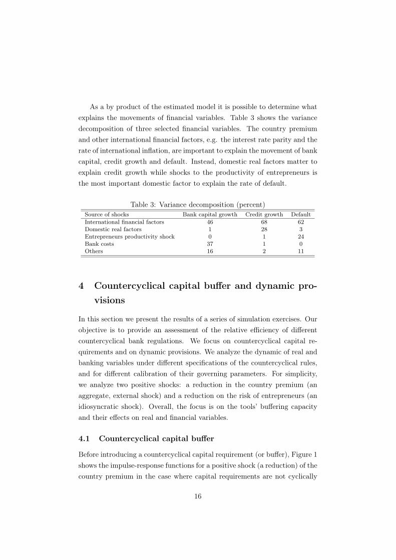
As a by product of the estimated model it is possible to determine whatexplains the movements of financial variables. Table 3 shows the variancedecomposition of three selected financial variables. The country premiumand other international financial factors, e.g. the interest rate parity and therate of international inflation, are important to explain the movement of bankcapital, credit growth and default. Instead, domestic real factors matter toexplain credit growth while shocks to the productivity of entrepreneurs isthe most important domestic factor to explain the rate of default.
Table 3: Variance decomposition (percent)Source of shocks Bank capital growth Credit growth DefaultInternational financial factors 46 68 62Domestic real factors 1 28 3Entrepreneurs productivity shock 0 1 24Bank costs 37 1 0Others 16 2 11
4 Countercyclical capital buffer and dynamic pro-visions
In this section we present the results of a series of simulation exercises. Ourobjective is to provide an assessment of the relative efficiency of differentcountercyclical bank regulations. We focus on countercyclical capital re-quirements and on dynamic provisions. We analyze the dynamic of real andbanking variables under different specifications of the countercyclical rules,and for different calibration of their governing parameters. For simplicity,we analyze two positive shocks: a reduction in the country premium (anaggregate, external shock) and a reduction on the risk of entrepreneurs (anidiosyncratic shock). Overall, the focus is on the tools’ buffering capacityand their effects on real and financial variables.
4.1 Countercyclical capital buffer
Before introducing a countercyclical capital requirement (or buffer), Figure 1shows the impulse-response functions for a positive shock (a reduction) of thecountry premium in the case where capital requirements are not cyclically
16

adjusted (notice that γREG does not change with the shock). The shock isexpansionary. Gross Domestic Product (GDP), consumption (C) and invest-ment (I) raise after the shock, which shows to have persistent effects. Thereduction in country risk affects the entrepreneurs relative cost of funding,reducing their leverage (leve) which determines a lower default rate (def).Bank credit (l) also expands but more slowly than GDP, which determinesthat during the 10 first quarters after the shock the ratio of credit to GDPfalls. Interestingly, if based on this ratio, a cyclically-adjusted bank capi-tal requirement would be procyclical rather than countercyclical! Indeed,the shock reduces the bank capital to asset ratio (N b/A) because banks arewilling to maintain a lower buffer above the minimum capital requirement(γBUFFER). This implies that, although bank capital (nb) increases, it doesless than bank assets.
Figure 1: Impulse-response functions: country risk premium shock
In Figure 2 we show the impulse-response functions for the same un-expected, positive shock to country premium when capital requirementsfollow a countercyclical rule based on the dynamic of real credit growth:γRt = γR0 + αRl (∆Lt −∆Lss), for three values of the parameter αRl . A firstobservation is that the introduction of this rule effectively raises the bankcapital requirement (γREG) during the period in which bank credit is expand-ing due to the positive external shock (15 quarters approximately). Second,
17

this impacts positively on bank capital, so that the ratio of bank capitalto bank assets fall less during the boom than without a cyclically-adjustedcapital requirement. Although there is no major effects on the capital buffer(γBUFFER) that banks are willing to maintain, the higher minimum capi-tal requirements implies an overall higher level of bank capital. Third, thehigher capital requirements due to the countercyclical capital rule do nothave major effects on real variables such as activity, consumption or in-vestment. Fourth, it does not have major effects on the dynamic of creditneither.
Figure 3 shows the results when the countercyclical capital rule is linkedto the dynamics of real GDP growth: γRt = γR0 +αRy (∆Yt−∆Yss). This caseshares the qualitative conclusions from the real credit growth rule: capitalrequirements raises in response to the shock implying higher bank capital-ization than in the benchmark case without major real effects. However,the raise in capital requirements takes place in a shorter period of time be-cause the growth rate of GDP is higher than that of credit over the first fourquarters after the shock. Moreover, on the more stringent calibrations ofthe countercyclical rule (αRy = 2.0) the ratio of bank capital to bank assetsraises instead of falling as in the benchmark case. This implies a higher cap-italization of the banking system. However, it is important to notice thathigher capital requirement (γREG) over a shorther period of time implies amore volatile desired capital buffer (γBUFFER).
We now turn the analysis to the case of an idiosyncratic, positive shock tothe riskiness of entrepreneurs (i.e. a reduction on the standard deviation σωof their distribution of risk). Figure 4 shows impulse and response functionsto this shock for the benchmark case with plain capital requirements, as wellas for the countercyclical capital requirement linked to real credit growth.The decrease on entrepreneurs’ riskiness has direct impact on the rate ofdefault, which in turn raises bank credit with a positive impact on activityand other real variables. Differently than in the case of a shock to countryrisk, in this case the ratio of credit to GDP increases. Overall, banks usetheir capital buffers to fund new loans, and just raises new capital after 5-10quarters, so that the ratio of bank capital to bank assets decreases.
The countercyclical capital requirement linked to real credit growth (γRt =
γR0 + αRl (∆Lt −∆Lss)) is effective to buffer bank capital during the periodin which the idiosyncratic shock persists. Indeed, in all calibrations of the
18
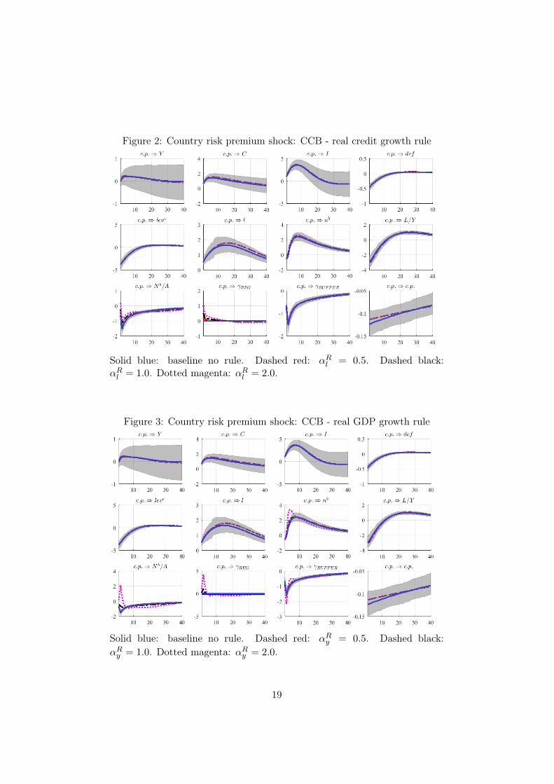
Figure 2: Country risk premium shock: CCB - real credit growth rule
Solid blue: baseline no rule. Dashed red: αRl = 0.5. Dashed black:αRl = 1.0. Dotted magenta: αRl = 2.0.
Figure 3: Country risk premium shock: CCB - real GDP growth rule
Solid blue: baseline no rule. Dashed red: αRy = 0.5. Dashed black:αRy = 1.0. Dotted magenta: αRy = 2.0.
19

Figure 4: Entrepreneurs risk premium shock: CCB - real credit growth rule
Solid blue: baseline no rule. Dashed red: αRl = 0.5. Dashed black:αRl = 1.0. Dotted magenta: αRl = 2.0.
rule the level of bank capital (nb) increases instead of staying constant overthe first quarters after the shock. However, there are not major effects onreal variables nor on bank credit.
Similar conclusions are reached when the countercyclical capital require-ment is linked to real GDP growth (see Figure 5). However, this rule is moresensitive than the former one to the calibration of the governing parameter.Indeed, by setting αRl = 2.0 bank capital rises to a point that allows anincrease of credit over the benchmark case, then adding more procyclicalityto the ratio of credit to GDP. Moreover, in this case the regulatory capi-tal requirement (γREG) and the in-excess desired level of capital by banks(γBUFFER) increase volatility with respect to the benchmark case.
4.2 Dynamic provisions
In this section we analyze the dynamics impulsed by the same shocks thatwere analyzed in the previous section but considering now a dynamic provi-sion rule for loan losses (i.e. LLPt = l0deftLt+l1(defss−deft)l0Lt) instead ofa countercyclical capital requirement. As in the previous section, we considerexpansionary shocks and focus the assessment on the buffering capacity of
20

Figure 5: Entrepreneurs risk premium shock: CCB - real GDP growth rule
Solid blue: baseline no rule. Dashed red: αRy = 0.5. Dashed black:αRy = 1.0. Dotted magenta: αRy = 2.0.
the regulatory tools.Figure 6 shows in solid blue lines the benchmark case were loan loss
provisions are static (i.e. LLPt = l0deftLt). The unexpected reduction inthe country risk premium translate into lower entrepreneurs’ leverage anddefault rates. In turn, given the static nature of the provision rule, currentperiod loan loss provisions (LLPt) fall, which adds procyclicality to finan-cial variables like, for example, bank credit. The introduction of a dynamiccomponent to the loan loss provision rule is effective to mitigate this procycli-cality. Moreover, loan loss provisions become countercyclical if the weightof the dynamic component on the rule is high enough. In this case, bankcapital (N b) and the ratio of bank capital to total assets (N b/A) are similarto those in the benchmark case. Nevertheless, the provision fund (LLRt)accumulates a buffer that may be used when the cycle reverts.
Differently than in the case of a countercyclical capital requirement, dy-namic loan loss provisions do have a countercyclical effect on real variables.This happens because the dynamic provision rule smooths the dynamics ofbank credit. During the boom, the provision rate increases, then it taxes theprovision of new credit, which in turn moderates credit expansion. After ap-
21

proximately twelve quarters, when the effect of the shock on entrepreneurs’default is over, the provision rate falls, then impulsing bank credit. In turn,this effects channels to real variables: the procyclicality of activity, consump-tion and investment falls. Interestingly, while the static provision rule makesactivity to fall below the steady-state level after several periods, the dynamicprovision rule reduces this risk.
Figure 6: Country risk premium shock: static vs. dynamic provisions
Solid blue: static provisions (l1 = 0). Dashed red: 1 = 0.5. Dashed black:1 = 1.0. Dotted magenta: 1 = 1.5.
Figure 7 shows the effects of an unexpected shock to the entrepreneurs’risk premium. Overall, the qualitative results of the country risk premiumshock case hold for the case of the shock to entrepreneurs’ risk premium.In particular, dynamic loan loss provisions are effective to mitigate the pro-cyclicality introduced by the shock and to build a reserve fund that maybe used to absorb future losses. Moreover, in this case dynamic provisionsachieve almost the stabilization of banks’ leverage (the inverse of the ratioN b/A) by moderating bank credit and slightly raising bank capital over thebenchmark with only static provisions.
The qualitative results from Figures 6 and 7 hold if we consider that thedynamic provision rule is linked to expected default, i.e. E(deft+1), insteadof current default, i.e. deft (see the Appendix).
22

Figure 7: Entrepreneurs risk premium shock: static vs. dynamic provisions
Solid blue: static provisions (l1 = 0). Dashed red: 1 = 0.5. Dashed black:1 = 1.0. Dotted magenta: 1 = 1.5.
5 Final remarks
With the aim of performing a realistic assessment of the countercyclical regu-lation promulgated in Basel III, and to compare its relative performance withother macroprudential policies already used in many countries, i.e. dynamicloan loss provisions, we develop a DSGE model for a small and open econ-omy. In the model, entrepreneurs’ default is endogenous particular attentionis put to the modeling of the banking sector and its prudential regulation.
The model is estimated using quarterly data for Uruguay in the period2005Q1 to 2015Q4. Uruguay has been using dynamic loan loss provisionssince 2001. Hence, this data provides a nice counterfactual for a realisticestimation of the proposed DSGE model.
The results suggest that both countercyclical capital buffers and dynamicprovisions are effective in generating buffers than may cover future losses.However, countercyclical capital requirements do not have major real effectswhile dynamic provisions may have. When the economy faces a positive,external shock, a countercyclical capital rule based on real GDP growth hasa quicker and stronger effect in buffering bank capital than a rule basedon real credit growth. In this case, the ratio of credit to GDP decreases,
23

which discourages the use of this variable to guide the buffering decision.In terms of smoothing the cycles, dynamic provisions seems to outperformcountercyclical capital requirements under external financial shocks.
Finally, the source of the shock matters to select the indicator variablefor the countercyclical capital requirement (credit to GDP does not seem ad-equate under external shocks), to calibrate the size of the dynamic provision-ing (the same calibration may be too countercyclical if the shock is domesticthan if it is external), and to select the policy tool (dynamic provisions seemsto outperform countercyclical capital requirements under external financialshocks). Hence, it seems prudent to have both policy tools available on theset of regulatory instruments.
24

Appendix
A Definition of variables
Table A.1: Exogenous processesv Households’ preference shocku Investment shockz Temporary TFP shocka Permanent TFP shockζ Country premium shockR∗ Foreign interest rateπ∗ Foreign inflation ratepCo∗ Commodities priceyCo Commodities endowmenty∗ Foreign GDPg Fiscal expendituresσω Std. dev. of entrepreneurs’ risk shocks Costs of banks’ assets substitutionγ Banks’ capital to assets ratioτ Banks’ reserve requirement
25

Table A.2: Selected endogenous variablesc Consumption mcH Home goods marginal costh Labor supply (hours) mcF Foreign goods marginal costhd Labor demand (hours) ∆H Hours dispersionw Wage ∆W Wage dispersionw Adjusters’ optimal wage ∆F Foreign good dispersion
mcW Labor marginal costs m ImportsrK Rent capital rate b∗ Banks bonds holdingsi Investment tb Trade balancek Entrepreneurs’ capital md Money demandπS Currency depreciation ma Households’ financial assetsq Price of entrepreneurs’ capital d Bank depositsy GDP Re Entrepreneurs’ returnyC Domestic absorption RD Deposits interest rateyF Foreign good supply RL Loans interest ratexF Foreign good demand yH Home composite goods supplyxH Domestic home good demand l Bank loansxH∗ Home good exports lev Entrepreneurs’ leverageR Monetary policy rate rp Entrepreneurs’ risk premiumξ Country premium ω Optimal thresholdπ Inflation rate def Default raterer Real exchange rate pH Home good pricepH Adjusters’ optimal home good price nB Predetermined banks’ capitalpF Foreign good price nB Banks’ capitalpF Adjusters’ optimal foreign good price ab Banks’ assetspY GDP deflator spr Spread on banks’ interest ratespen Banks’ capital penalty llr Loan loss reserve fundllu Loan loss utilization cost Banks’ costsλ Lagrange multiplier
26

B Equilibrium conditions
Given initial values and exogenous sequences
{vt, ut, zt, at, ζt, R∗t , π∗t , pCo∗t , yCot , y∗t , gt, πTt , σω,t, st, γt, τt}∞t=0,
the following conditions are satisfied at the equilibrium:
Households:
λt =
(ct − ς
ct−1
at−1
)−1
− βςEt{vt+1
vt(ct+1at − ςct)−1
}, (E.1)
wtmcWt = κ
hφtλt, (E.2)
λt =β
atRtEt
{vt+1
vt
λt+1
πt+1
}, (E.3)
λt =β
atR∗t ξtEt
{vt+1
vt
πSt+1λt+1
πt+1
}, (E.4)
fWt = mcWt w−εWt hdt+βθWEt
{vt+1
vt
λt+1
λt
(πϑWt (πTt+1)1−ϑW
πt+1
)−εW (wtwt+1
)−εW ( wtwt+1
)−1−εWfWt+1
}.
(E.5)
fWt = w1−εWt hdt
(εW − 1
εW
)+βθWEt
{vt+1
vt
λt+1
λt
(πϑWt (πTt+1)1−ϑW
πt+1
)1−εW (wtwt+1
)1−εW ( wtwt+1
)−εWfWt
}.
(E.6)
1 = (1− θW )w1−εWt + θW
(wt−1
wt
πϑWt−1(πTt )1−ϑW
πt
)1−εW
. (E.7)
∆Wt = (1− θW )w
−εW
t + θW
(wt−1
wt
πϑWt−1(πTt )1−ϑW
πt
)−εW∆Wt−1. (E.8)
ht = hdt∆Wt . (E.9)
mat =
[(1− oM )
1ηM (rertdt)
ηM−1ηM + o
1ηM
M
(mdt
) ηM−1ηM
] ηMηM−1
(E.10)
λt(1−R−1t ) = νt (ma
t )−1+ 1
ηM o
1ηM
M
(mdt
) −1ηM (E.11)
λt
(1− RDt
R∗t ξt
)= νt (ma
t )−1+ 1
ηM (1− oM )
1ηM
(rertdt)−1ηM (E.12)
Aggregate Consumption:
yCt =
[(1− o)
1η
(xHt
) η−1η
+ o1η(xFt
) η−1η
] ηη−1
, (E.13)
xFt = o(pFt
)−ηyCt , (E.14)
xHt = (1− o)(pHt
)−ηyCt , (E.15)
27

Home goods:
mcHt =1
αα (1− α)1−α(rKt )αw1−α
t
pHt zta1−αt
, (E.16)
kt−1
hdt= at−1
α
1− αwtrKt
, (E.17)
yHt ∆Ht = zt
(kt−1
at−1
)α(ath
dt )
1−α, (E.18)
fHt =(pHt
)−εHyHt mc
Ht +βθHEt
{vt+1
vt
λt+1
λt
(πϑHt (πTt+1)1−ϑH
πt+1
)−εH (pHtpHt+1
)−εH ( pHtpHt+1
)−1−εHfHt+1
},
(E.19)
fHt =(pHt
)1−εHyHt
(εH − 1
εH
)+βθHEt
{vt+1
vt
λt+1
λt
(πϑHt (πTt+1)1−ϑH
πt+1
)1−εH (pHtpHt+1
)1−εH ( pHtpHt+1
)−εHfHt+1
},
(E.20)
1 = θH
(pHt−1
pHt
πϑHt−1(πTt )1−ϑH
πt
)1−εH
+ (1− θH)(pHt
)1−εH, (E.21)
∆Ht = (1− θH)
(pHt
)−εH+ θH
(pHt−1
pHt
πϑHt−1(πTt )1−ϑH
πt
)−εH∆Ht−1, (E.22)
Import Agents:
1 = θF
(pFt−1
pFt
πϑFt−1(πTt )1−ϑF
πt
)1−εF
+ (1− θF )(pFt
)1−εF. (E.23)
∆Ft = (1− θF )
(pFt
)−εF+ θF
(pFt−1
pFt
πϑFt−1(πTt )1−ϑF
πt
)−εF∆Ft−1. (E.24)
mcFt = rert/pFt . (E.25)
fFt =(pFt
)−εFyFt mc
Ft +βθFEt
{vt+1
vt
λt+1
λt
(πϑFt π1−ϑF
πt+1
)−εF (pFtpFt+1
)−εF ( pFtpFt+1
)−1−εFfFt+1
}.
(E.26)
fFt =(pFt
)1−εFyFt
(εF − 1
εF
)+βθFEt
{vt+1
vt
λt+1
λt
(πϑFt (πTt+1)1−ϑF
πt+1
)1−εF (pFtpFt+1
)1−εF ( pFtpFt+1
)−εFfFt+1
}.
(E.27)mt = yFt ∆F
t . (E.28)
Investment:
kt = (1− δ)kt−1
at−1+
[1− γ
2
(itit−1
at−1 − a)2]utit, (E.29)
1
qt=
[1− γ
2
(itit−1
at−1 − a)2
− γ(
itit−1
at−1 − a)
itit−1
at−1
]ut
+β
atγEt
{vt+1
vt
λt+1
λt
qt+1
qt
(it+1
itat − a
)(it+1
itat
)2
ut+1
}. (E.30)
28

Entrepreneurs:Retπt
=rKt + qt(1− δ)
qt−1. (E.31)
RLt lt−1rert−1πSt = gt−1(ωt)R
etqt−1kt−1, (E.32)
qtkt = nt + ltrert, (E.33)
levt =qtktnt
, (E.34)
Et
{Ret+1
[ht(ωt+1)− h′t(ωt+1)gt(ωt+1)
g′t(ωt+1)
]}= Et
{h′t(ωt+1)
g′t(ωt+1)RLt+1π
St+1
}, (E.35)
rpt = Et {Ret+1} /Et{RLt πSt+1}, (E.36)
nt = ϑ
{Ret
qt−1
πt
kt−1
at−1ht−1(ωt)
}+ ιe, (E.37)
RLt−1lt−1rert−1πSt = ωtR
etqt−1kt−1, (E.38)
deft = Φ
(ln(ωt) + .5σ2
ω,t−1
σω,t−1
), (E.39)
mont = [1− ht−1(ωt)− gt−1(ωt)]Retqt−1kt−1. (E.40)
Banks:
lt + b+ llpt = (1− τt)dt + nbt , (E.41)
at−1nbt = RLt lt−1 + bt−1R
∗t ξt + llut − (RDt−1 − τt−1)dt−1, (E.42)
at−1llut = min{
(RLt−1 − RLt )lt−1, llrt−1 + llpt−1
}, (E.43)
at−1abt = RLt lt−1 + bt−1R
∗t ξt + at−1llut + τt−1dt−1, (E.44)
llrt =(llrt−1 + llpt−1)
at−1− llut, (E.45)
Et
{β
at
vt+1
vt
λt+1πSt+1
λtπt+1
[∂nbt+1
∂Lt− ∂pent+1
∂Lt
]}= stS
LLt, (E.46)
Et
{β
at
vt+1
vt
λt+1πSt+1
λtπt+1
[∂nbt+1
∂Bt− ∂pent+1
∂Bt
]}= stBt. (E.47)
RDt =RDt − τt1− τt
, (E.48)
pent =φD2
(nbtabt− γt−1
)2
nbt , (E.49)
nbt =ϑB
πt
[nbt − pent − costt−1
]+ ιBnb, (E.50)
sprt = RLt /RDt , (E.51)
costt = st(SLl2t + b2t ). (E.52)
Rest of the world:
xH∗t = o∗(pHtrert
)−η∗y∗t , (E.53)
29

ξt = ξ exp
[−ψ
(rertb
∗t − rer × b∗
rer × b∗
)+ζt − ζζ
], (E.54)
Policy:
RtR
=
(Rt−1
R
)ρR [( πtπTt
)απ (yty
)αy (πStπS
)απS]1−ρR
exp(εRt ), (E.55)
Aggregation and Market clearing:
yHt = xHt + xH∗t , (E.56)
yCt = ct + it + gt +mont, (E.57)
rertrert−1
=πSt π
∗t
πt. (E.58)
yt = ct + it + gt + xH∗t + yCot −mt, (E.59)
tbt = pHt xH∗t + rertp
Co∗t yCot − rertmt, (E.60)
rertb∗t = rert
b∗t−1
at−1π∗tR∗t−1ξt−1 + tbt − (1− χ)rertp
Co∗t yCot , (E.61)
pYt yt = ct + it + gt + tbt. (E.62)
yFt = xFt . (E.63)
30

C Extra figures
Figure C.1: Dynamic provisions with country risk premium shock: currentvs. expected default
10 20 30 40-0.2
0
0.2
0.4c.p. ⇒ Y
10 20 30 400.5
1
1.5
2c.p. ⇒ C
10 20 30 40-2
0
2
4c.p. ⇒ I
10 20 30 40-0.5
0
0.5c.p. ⇒ def
10 20 30 40-4
-2
0
2c.p. ⇒ leve
10 20 30 400
1
2c.p. ⇒ L
10 20 30 40-2
0
2
4c.p. ⇒ N b
10 20 30 40-4
-2
0
2c.p. ⇒ L/PIB
10 20 30 40-1.5
-1
-0.5
0c.p. ⇒ N b/A
10 20 30 40-0.4
-0.2
0
0.2c.p. ⇒ LLP
10 20 30 400
0.5
1
1.5c.p. ⇒ LLR
10 20 30 40-0.12
-0.1
-0.08c.p. ⇒ c.p.
Solid blue: current default (j = t). Dashed red: expected default (j = t+1).Both l1 = 0.5.
31

Figure C.2: Dynamic provisions with entrepreneurs risk premium shock:current vs. expected default
10 20 30 40-0.05
0
0.05
0.1σω ⇒ Y
10 20 30 400
0.01
0.02σω ⇒ C
10 20 30 40-0.1
0
0.1
0.2σω ⇒ I
10 20 30 40-1
-0.5
0
0.5σω ⇒ def
10 20 30 40-0.2
0
0.2σω ⇒ leve
10 20 30 400
0.1
0.2
0.3σω ⇒ L
10 20 30 400
0.02
0.04σω ⇒ N b
10 20 30 40-0.1
0
0.1
0.2σω ⇒ L/PIB
10 20 30 40-0.15
-0.1
-0.05
0σω ⇒ N b/A
10 20 30 40-1
-0.5
0
0.5σω ⇒ LLP
10 20 30 400
1
2σω ⇒ LLR
10 20 30 40-15
-10
-5
0σω ⇒ σω
Solid blue: current default (j = t). Dashed red: expected default (j = t+1).Both l1 = 0.5.
32

References
Agénor, P.-R., Pereira da Silva, L., 2017. Cyclically adjusted provisions andfinancial stability. Journal of Financial Stability 28, 143–162.
Agénor, P.-R., Zilberman, R., 2015. Loan loss provisioning rules, procyclical-ity, and financial volatility. Journal of Banking and Finance 61, 301–315.
Allen, L., Rai, A., 1996. Bank charter values and capital levels: An inter-national comparison. Journal of Economics and Business 48 (3), 269 –284.
Ayuso, J., Perez, D., Saurina, J., 2004. Are capital buffers pro-cyclical?evidence from spanish panel data. Journal of Financial Intermediation13 (2), 249–264.
Barth, J., Caprio, G., Levine, R., 2006. Rethinking Bank Regulation: TillAngels Govern. Cambridge University Press.
Basal, J., Carballo, P., Cuitiño, F., Frache, S., Licandro, G., Mourelle, J.,Rodríguez, H., Rodriguez, V., Vicente, L., 2016. Un modelo estocástico deequilibrio general para la economía uruguaya. Documento de trabajo delBCU.
Berger, A., DeYoung, R., Flannery, M., Oztekin, O., 2008. How do largebanking organizations manage their capital ratios? Journal of FinancialServices Research 34 (2), 123–149.
Bernanke, B., Gertler, M., Gilchrist, S., 1999. The financial accelerator ina quantitative business cycle framework. In: Taylor, J., Woodford, M.(Eds.), Handbook of Macroeconomics. Elsevier, Ch. 21, pp. 1341–1393.
Bouvatier, V., Lepetit, L., 2012. Provisioning rules and bank lending: Atheoretical model. Journal of Financial Stability 8, 25–31.
Christiano, L., Motto, R., Rostagno, M., 2014. Risk shocks. American Eco-nomic Review 104 (1), 27–65.
Chui, M., Kuruc, E., Turner, P., 2016. A new dimension to currency mis-matches in the emerging markets: non-financial companies. BIS Workingpaper 550.
33

Darracq-Pariès, M., Kok-Sørensen, C., Rodriguez-Palenzuela, D., 2011.Macroeconomic propagation under different regulatory regimes: Evidencefrom an estimated dsge model for the euro area. International Journal ofCentral Banking 7 (4), 49–113.
Fonseca, A., Gonzalez, F., 2009. How bank capital buffers vary across coun-tries: The influence of cost of deposits, market power and bank regulation.Journal of Banking and Finance.
Gerali, A., Neri, S., Sessa, L., Signoretti, F., 2010. Credit and banking in adsge model of the euro area. Journal of Money, Credit and Banking 42 (1),107–141.
Glocker, C., Towbin, P., 2012. Reserve requirements for price and finan-cial stability: When are they effective? International Journal of CentralBanking 8 (1), 65–114.
Gómez, F., Ponce, J., 2015. Regulation and bankers’ incentives. BCU Work-ing Paper 5.2015.
Goodhart, C., Sunirand, P., Tsomocos, D., 2006. A model to analyse financialfragility. Economic Theory 27, 107–142.
Jiménez, G., Ongena, S., Peydró, J.-L., Saurina, J., Forth. Macroprudentialpolicy, countercyclical bank capital buffers, and credit supply: Evidencefrom the spanish dynamic provisioning experiments. Journal of PoliticalEconomy.
Jokipii, T., Milne, A., 2008. The cyclical behaviour of european bank capitalbuffers. Journal of Banking & Finance 32 (8), 1440–1451.
Jokipii, T., Milne, A., 2011. Bank capital buffer and risk adjustment deci-sions. Journal of Financial Stability 7 (3), 165–178.
Lindquist, K.-G., 2004. Banks buffer capital: how important is risk. Journalof International Money and Finance 23 (3), 493–513.
Milne, A., Whalley, E., 2001. Bank capital regulation and incentives forrisk-taking. Cass business School Research Paper.
Peura, S., Jokivuolle, E., 2004. Simulation based stress tests of banks’ regu-latory capital adequacy. Journal of Banking & Finance 28 (8), 1801–1824.
34
Stolz, S., Wedow, M., 2011. Banks’ regulatory capital buffer and the busi-ness cycle: evidence for german savings and cooperative banks. Journal ofFinancial Stability 7, 98–110.
Tobal, M., 2013. Currency mismatch: New database and indicators for latinamerica and the caribbean. CEMLA Research paper.
VanHoose, D., 2008. Bank capital regulation, economic stability, and mone-tary policy: What does the academic literature tell us? Atlantic EconomicJournal 36 (1), 1–14.
35
