could indonesian sfas 50 and 55 (revised 2006) reduce ... · 4 pedoman akuntansi perbankan...
TRANSCRIPT

1
Could Indonesian SFAS 50 and 55 (Revised 2006) Reduce
Earnings Management of Commercial Banks in Indonesia?
Yossi Diantimala
Ph.D Student of Faculty of Economic and Business of University of Gadjah Mada
Lecturer of University of Syiah Kuala
Zaki Baridwan
Professor of Faculty of Economic and Business of University of Gadjah Mada
Abstract
This paper aims to examine the ability of accounting standard statements to reduce
earnings management of commercial banks in Indonesia. The specific purposes of this
research are to examine, first, income smoothing behavior of bank managers through the
allowance for impairment loss, second, the impact of the implementation of Indonesian SFAS
50 and 55 (revision 2006) on reducing income smoothing of reported earnings of commercial
banks in Indonesia, and third, income smoothing behavior of commercial banks in quarterly
earnings.
The sample used in this research is 28 publicly commercial banks in Indonesia for the
periods 2008:I until 2011:IV. Overall, there are 448 bank-quarter observations and 112 bank-
annual observations. Unlike prior studies that rely primarily on time-series models or cross
sectional models, we focus on the specification of panel time series cross-sectional models of
the allowance for impairment loss and earnings before tax and allowance using quarterly and
annual data. In addition, we examine differences in the power of current accrual models in
detecting earnings management across audited and unaudited quarters. T-test of fixed effects
model of panel data is used to test hypothesis 1 and t-test two sample means is used to test
hypothesis 2. The results show that commercial bank managers manage their reported
earnings through the allowance for impairment loss. The implementation of SFAS 50 and 55
(revised 2006) is not significant to reduce the level of earnings management.
Keywords: Indonesian SFAS 50 and 55 (Revised 2006), IAS 32 and 39, earnings
management, the allowance for impairment loss, loan loss provision, and earnings before tax
and allowance.
Introduction
The accounting literatures stated that business firm’s managers, including bank
managers, manage their reported earnings for many different purposes. The best devices for
managers to manage earnings are through accrual accounts (Healy and Wahlen, 1999). In
2
addition, financial reporting standards require that bank managers estimate loan loss
provisions (hereafter, LLP) to reflect changes in expected future loan losses. A loan loss
provision is an allowance formed to anticipate loan losses in the future. This allowance is a
non-cash expense to anticipate a possible loss in value of loan outstanding, therefore, it is the
biggest accrual of a commercial bank.
Technically, the LLP1 is the amount expensed on the income statement. The way bank
managers justify their allowance for loan and losses as accrual, may largely affect their
reported earnings. The amount of Allowance for loan loss estimated by managers may
increase or decrease the amount of reported earnings. Higher the allowance, the earnings is
getting smaller. Otherwise, smaller the allowance, the earnings is getting higher.
Indonesian SFAS (we call PSAK) 50 and 55 regulate how a bank should treat the LLP.
The old accounting standards2 for commercial banks in Indonesia allowed banks to use their
judgment in determining the amount of the allowance for impairment loss. Consequently,
banks have substantial flexibility in determining lower or higher allowance for impairment
losses for this period in order to accommodate their motivations. Nevertheless, at present, all
commercial banks must adjust their allowance for impairment loss computation to Indonesian
statements of financial accounting standards (Indonesian SFAS) 50 and 55 (revised 2006).
The implementation of the new SFAS3 might cause earnings management through allowance
for impairment loss becoming more difficult for banks managers. Banks do not have
flexibility in determining the amount of loan loss provisions because, according to the SFAS,
1 For Indonesian banks, the term of LLP is allowance for impairment losses. 2 PSAK 50, “Accounting for Investments in Certain Securities,” and 55 (Revised 1999), “Accounting for
Derivatives and Hedging Activities.” 3 The statements have been in operative since January 1st 2009. But, since almost all banks were not ready to
implement the PSAK 50 and 55 (revision 2006) yet, the effective date was delayed until January 1st 2010.
3
loan are impaired when objective evidence demonstrates that a loss event has occurred after
the initial recognition of the asset, and that the loss event has an impact on the future cash
flow on the asset which can be estimated reliably. The impairment of loan is calculated
individually based on the probability of a loan to become loss4. On one side, a good quality
loan will reduce the impairment, whereas a bad quality loan will increase the impairment.
Therefore, it would effectively limit the ability of bank managers to use their judgment in
determining the amount of the allowance.
Regarding bank managers’ behavior to smooth income, there are three issues that are
still debated today that motivate this study. First, it is about the role of LLP as a tool for
managers to manage their reported earnings. Ma (1988), Kanagaretnam et al. (2003),
Anandarajana et al. (2003, 2007); Eng and Nabar (2007); and Pinho and Martins (2009) find
that bank managers use loan loss provisions to smooth their income. Conversely, Wetmore
and Brick (1994), Beatty et al. (1995), and Ahmed et al. (1999) find no association
between loan loss provision and earnings management by the banks in their sample. These
contradicting results motivate us to empirically examine managers’ devices to manage their
reported earnings.
Second, it is about the impact of changes in accounting standards on income
smoothing. SFAS 50 and 55 (revised 2006) are accounting standards which have been
converged to IFRS, specifically, IAS 32 and 395. Therefore, commercial banks in Indonesia
have implemented internationally accounting standards. The arguments about the ability of
IFRS to reduce earnings management are mixed. One argument asserts that IFRS provides
4 Pedoman Akuntansi Perbankan Indonesia (PAPI) 2008 (accounting guideline for Indonesian commercial banks
published by Central Bank of Indonesia). 5 IAS 32 Financial instruments: presentation and IAS 39 Financial instruments: recognition and measurement.
4
more opportunities for managers to use accruals to manipulate earnings, particularly in
emerging economies such as in China (Zhou et al., 2009) and India (Rudra and Bhattacharjee,
2012). In both countries, firms adopting IFRS appear to be more likely to smooth earnings
compared with firms that do not. In contrast, in developed countries, firms adopting IFRS are
less likely to smooth their income (Barth et al., 2005). These contradicting arguments provide
a strong basis for us to empirically examine the impact of new accounting standards, or
changes in accounting standards, on the earnings management behavior of firms.
The third motivation is about the pattern of quarterly earnings and annual earnings as
an indicator of earnings management. The empirical evidences demonstrate that series of
quarterly earnings is useful in predicting future annual earnings (Hopwood, et al., 1982),
therefore, it is resonable enough to claim that bank managers have incentive to maintain the
stability of quarterly earnings. However, the evidence on the quarterly patterns in earnings
distributions is somewhat conflicting. While Kerstein and Rai (2007) and Jacob and
Jorgensen (2007) find that the effort to minimize the variation in earnings is strongest in the
fourth quarter, Brown and Pinello (2007), however, find that the effort of management to
manage their income has been started in interim quarters in order to avoid small negative
analyst forecast errors. The first two studies examine small profit firms while Brown and
Pinello (2007) examine firms that avoid missing analyst forecast targets. Differences in the
incentives and opportunities may be caused by differences in bank performance. Poor-
performing banks tend to increase earnings in the fourth quarter to meet the level of required
accounting earnings, while banks that perform well during the interim period will reduce
earnings in the fourth quarter to form a reserve in the future (Das et al., 2009).

5
Based on the phenomena and motivations above, this research is aimed to examine the
ability of SFAS (PSAK) 50 and 55 (revision 2006) to reduce earnings management. The
specific purpose of this research is to examine, first, income smoothing behavior of bank
managers through the allowance for impairment loss, second, the impact of the
implementation of Indonesian SFAS 50 and 55 (revision 2006) on reducing income
smoothing of reported earnings of commercial banks in Indonesia, and third, income
smoothing behavior of commercial banks in quarterly earnings.
By applying Indonesian SFAS 50 and 55 (revised 2006) which has been converged to
IAS 32 and IAS 39, commercial banks in Indonesia must use the “fair value” method in
estimating the amount of loan loss provisions or allowance for impairment loss. Since all
Indonesian firms formally adopted IFRS on January 1, 2012, this study provides preliminary
research for future researches on the impact of IFRS with fair value method on earnings
management practice, firm value, and business decision making in Indonesia. This study is
also give a significant contribution for standard setter, the capital market supervisory agency
(BAPEPAM), and investors concerning the ability of accounting standards to reduce earnings
management.
Additionally, this study has a considerable contribution for methodological approach.
Unlike prior studies that rely primarily on time-series or cross sectional models, this study
concentrates on the specification of panel time series cross-sectional models of the allowance
for impairment loss, and earnings before tax and allowance using quarterly and annual data.
Furthermore, we examine differences in the power of current accrual models in detecting
earnings management across audited and unaudited quarterly earnings. The considerations of
using panel data over conventional cross sectional or time series data set are, first, it allows us

6
to test and relax the assumptions that are implicit in cross sectional analysis (Maddala and
Lahiri, 2009: 583). Second, panel data usually give us a large number of data point, increasing
the degree of freedom and reducing the problem of collinearity among explanatory variables,
hence improving the efficiency of econometrics estimates to get more precise estimates. More
importantly, panel data allow us to analyze a number of important economic questions that
cannot be addressed using cross sectional or time series data set (Hsiao, 2003:3).
The last contribution is this study employ both annual and quarterly earnings to
examine whether the pattern of quarterly earnings can potentially serve as an indicator of
earnings management (Das et al., 2009). The evidence on the quarterly patterns in earnings
distributions is somewhat conflicting. Therefore, the result of this study can be an empirical
support on the relationship between quarterly earnings and income smoothing in accounting
literature.
The Related Theory and Hypothesis Development
Agency Theory and Income Smoothing Hypothesis
The issue of earnings management is always interesting to study because the issue is
related to the behavior of managers who take advantage of their position as supreme
regulators of firm policies. This behavior is always against the wishes of owners who also
want to benefit from the entity that is managed by managers. Therefore, regulatory bodies
such as standard setters and capital market supervisors are always trying to balance the
interest of both parties, a manager of a firm as an agent and the owner of the firm as the
principal, by issuing new accounting standards or strengthening the existing standards in order
to achieve certain social objectives.
7
Different interest of principal, agent, and regulator are described in agency theory.
This theory is used as the basis for the development of this study. In his paper, Liang (2004)
develops earnings management model which illustrates the interaction among managers,
shareholders, and regulatory bodies, specifically standard setters, in an equilibrium condition
and in the labor market. He calls them self-interested economic agents. Based on this model,
he concludes that when selecting the optimal accounting standards, the regulator may face a
conflict between the two objectives of reducing agency costs and increasing the valuation
information content in the accounting report. In short, the equilibrium earnings management
reflects various economic trade-offs.
The behavior of managers to meet their objectives can also be viewed from the
income-smoothing hypothesis. Management seeks to reduce the variability in the trend of
reported earnings with subjective accounting judgments. Such reductions are achieved by
shifting certain revenue or expense items so that year-to-year earnings are less variable. The
rationale for income smoothing can be traced to internal and external factors of a firm such as
compensation motives, accounting standards and accounting considerations, market demands,
and regulatory demands (Greenawalt and Sinkey,1988). These factors drive owner and
managers to position reported earnings. Greenawalt and Sinkey (1988) used income
smoothing hypothesis to explain the income smoothing behavior of bank managers.
According to Greenawalt and Sinkey (1988), in banking, the analysis of the provision for loan
losses (an expense) and of its corresponding balance-sheet entry, the allowance for loan losses
(also called the bad-debt reserve) is important because (1) the former affects both the amount
and the timing of reported earnings and (2) the latter reflects management's judgment of
future loan losses, a crude measure of loan quality. The perfect nature of loan-loss estimates

8
as a smoothing device is the judgment of bank manager in determining the allowance for loan
loss and in estimating the current amount of loans that will not be collected.
Loan Loss Provision and income Smoothing
Income smoothing is the most interesting earnings management pattern (Scott, 2009:
405). The investigations of the role of loan loss provision as the best device for managers to
manage their earnings give contradicting results. Ma’s study (1988) determines whether U.S.
commercial banks utilize loan loss provision (LLP) as a device to smooth reported earnings.
He concluded that LLP, together with loan charge-offs, were used by banks for income
smoothing. Bhat (1996) examines the income smoothing hypothesis for large banks in Texas
that reported their earnings over the period 1981-1991. He analyzes whether banks use loan-
loss provisions to manipulate earnings. His empirical result suggests that banks with close
relationships between their loan-loss provisions and their earnings before loan-loss provisions
but after taxes do tend to smooth earnings. Kanagaretnam et al. (2003) investigate the
predictions of the Fudenberg-Tirole model by examining whether bank managers smooth
income through LLP. Their empirical analysis is based on 4,166 bank-quarter observations.
The sample consists of US bank holding companies for the period 1987 to 2000. Quarterly
information is obtained from the Call Reports filed by bank holding companies with the
Federal Reserve Banks. Their result shows that banks’ managers use LLP to smooth their
income.
Parallel to the studies above, Anandarajana et al. (2007) demonstrate that banks in
Australia use loan loss provisions to manage earnings. Further, listed commercial banks
engage more aggressively in earnings management using loan loss provisions (LLPs) than
9
other banks. They also find that earnings management behavior was more pronounced after
implementation of the Basel Accord, and Anandarajana et al. (2003) find that Spanish banks
more aggressively engage in earnings management through LLP since Basel I was introduced.
Relatedly, Bornemann et al. (2010) investigate income smoothing behavior of German banks
for the period 1995 through 2009 and conclude that bank managers can potentially avoid
reporting small declines in earnings by underestimating the reserve to provision to avoid
negative net income and reduce the volatility of net income over time.
On the contrary, Wetmore and Brick (1994) study factors that might be associated
with income smoothing by banks, and find no evidence that loan loss provision is used as a
tool for earnings management. Beatty et al. (1995) considers whether 752 domestic US banks
for the period 1987 (1986 year-end) through 1990 (1989 year-end) alter timing and magnitude
of transactions and accruals to achieve earnings management, but find no association between
loan loss provision and earnings management. Ahmed et al. (1999), the only study to use data
that include the period after the change in capital adequacy regulations, investigate 113 US
bank holding companies for the period 1986-1995, also find no evidence that banks used loan
loss provision to manage earnings. Their finding of no association was unexpected, since the
capital adequacy regulation eliminated the costs of earnings management.
Evidence of income smoothing behavior through loan loss provisions of Asian banks
is represented by Eng and Nabar’s (2007) study. They examine the behavior of loan loss
accounting disclosure of banks in Hong Kong, Malaysia, and Singapore from 1993 through
2000. They also examine whether Asian bank investors view unexpected loan loss provision
to be positive or negative. They focus on banks in Hong Kong, Malaysia, and Singapore, as
these countries follow the Anglo-Saxon accounting model, and therefore share similarities in

10
their accounting principles. These three countries were British colonies, and their accounting
systems were initially based on the UK model. Their results indicate that unexpected loan loss
provisions are positively related to bank stock returns and future cash flows. These results
suggest that Asian bank managers use loan loss provision to smooth income and Asian bank
investors reacted to these provisions in a fashion similar to that documented by Wahlen
(1994) for US banks.
In the case of commercial banks in Indonesia, allowance for impairment loss is the
term used to illustrate loan loss provision. The meaning and accounting procedures of the
allowance for impairment loss is equal to loan loss provision.
H1: Managers of Indonesian banks smooth their income through allowance for impairment
losses.
The SFAS 50 and 55 (revised 2006)
The SFAS 50 (revised 2006) deals with presentation and disclosures of financial
instruments and the SFAS 55 (revised 2006) copes with recognition and measurement of
financial instruments. The crucial rule in both SFAS is that credit, as well as bank assets is
classified as loan and receivables. Loan and receivables are initially recognized at fair value
plus transaction costs and subsequently measured at amortized cost using the effective interest
rate method. In the case of impairment, the impairment loss is reported as deduction from the
carrying value of the financial assets classified as loans and receivables recognized in the
income statements as allowance for impairment losses. At each balance sheet date, the bank
assesses whether there is objective evidence that loans which are not carried at fair value
through income statement are impaired. Loans are impaired when objective evidence

11
demonstrates that a loss event has occurred after the initial recognition of the assets, and that
the loss event has an impact on the future cash flows of the assets which can be estimated
reliably.
The bank considers evidence of impairment for loans measured at amortized cost
individually and collectively. All individual loans are assessed for specific impairment. All
individual loans measured at amortized cost found not to be specifically impaired are then
collectively assessed for any impairment that has been incurred but not yet identified. Loans
that are not individually significant are collectively assessed for impairment by grouping
together such financial assets with similar risk characteristic. Collective allowance6 for loans
classified as current, special mention, substandard, doubtful and loss are calculated after
deducting the value of allowable collateral in accordance with Bank Indonesia regulations.
The calculation of allowance for impairment losses is based on carrying amount (amortized
cost)7.
Impairment losses on financial assets carried at amortized cost are measured as the
difference between the carrying amount of the financial assets and the present value of
estimated future cash flows discounted at the financial assets’ original effective interest rate.
6 In assessing collective impairment, the bank applies Bank Indonesia Circular Letter No. 11/33/DPNP dated
December 8th 2009, “The Amendment to the Bank Indonesia Circular Letter No. 11/4/DNDP dated January
27th 2009 on the Implementation of Accounting and Reporting Guidelines for Indonesian Banking Industry”.
The Bank Indonesia Circular Letter contains the amendment to PAPI 2008 regarding the transitional provision
on estimation of collective impairment of loans for eligible banks.
In accordance with the Appendix to the Bank Indonesia Circular letter No. 11/33/DNDP dated December 8th
2009, the allowance for collective impairment losses of loans refers to the general allowance and specific
allowance in accordance with the Bank Indonesia regulations regarding the assessment of commercial banks’
assets quality as follows:
1. Current: minimum of allowance for impairment losses 1%.
2. Special Mention: minimum of allowance for impairment losses 5%. 3. Substandard: minimum of allowance for impairment losses 15%.
4. Doubtful: minimum of allowance for impairment losses 50%.
5. Loss: minimum of allowance for impairment losses 100%.
7 All statements in this phrase are summarized from PAPI (2008).

12
Calculating the present value of estimated future cash flows of financial assets with collateral
reflects the cash flows that can be generated from the acquisition of collateral, minus the cost
for obtaining and selling the collateral, regardless of whether the takeover is likely to happen
or not. Losses are recognized in the income statement and reflected in an allowance account,
namely allowance for impairment loss, against financial assets carried at amortized cost.
Interest on the impaired financial assets continues to be recognized using the rate of interest
used to discount the future cash flows for the purpose of measuring the impairment loss.
When a subsequent event causes the amount of impairment loss to decrease, the impairment
loss is reversed through the income statement8.
Accounting Standards and Income Smoothing
SFAS 50 and 55 (revised 2006) are accounting standard statements which have been
converged to IFRS, specifically, IAS 32 and 399. The main objective of the Indonesian
standard setters to converge the statements is to tighten accounting standards in order to
restrict or to reduce earnings management and to provide more relevant information to the
capital market. This is reasonable because the prior accounting standard provide a chance for
managers or auditors to judge the amount to be reported. By tightening the standards,
managers’ or auditors’ judgment can be limited by requiring evident measurement and by
proving better rules or exhaustive guidance (Ewert and Wagenhofer, 2005). However, there
are also arguments that IFRS provides more opportunities for managers to use accruals to
manipulate earnings, particularly in emerging economy such as in China (Zhou et al., 2009)
and India (Rudra and Bhattacharjee, 2012). These firms adopting IFRS appear to be more
8 All statements in this phrase are summarized from PAPI (2008). 9 IAS 32 Financial instruments: presentation and IAS 39 Financial instruments: recognition and measurement.

13
likely to smooth earnings compared with firms that do not. In contrast, in developed countries,
firms adopting IFRS are less likely to smooth income (Barth et al., 2005).
These conflicting results are caused by the timing of IFRS adoption of sample firms.
Rudra and Bhattacharjee (2012) use firms adopting IFRS earlier than firms in Barth’s et al.
study. The tendency to manage earnings occurred in the early adoption of new standard
statements. Firms which have to adopt new standards use the timing of adoption and the
choice of transition method to manage their earnings (Gujarathi and Hoskin, 1992; Smith and
Rajaee, 1995).
This conflict is reinforced by studies of Stefanescu (2006) and Oosterbosch (2009).
Stefanescu (2006) investigate the impact of new accounting standards, SFAS 144
“Accounting for the Impairment or Disposal of Long-Lived Assets” (FASB 2001) on
income smoothing through the timing of asset sales. She finds that income smoothing
behavior through the timing of asset sales is lessened in the post-SFAS 144 reporting regime.
Oosterbosch (2009) examines first whether the level of earnings management by banks
through loan loss provisioning has decreased since the IFRS-adoption, and second, whether
loan loss disclosure requirements are negatively related to banks’ income smoothing. He uses
a sample of European banks and a single-stage regression that models the non-discretionary
part of LLPs and tests for income smoothing. The results show that the level of earnings
management has indeed decreased since IFRS adoption. However, evidence suggested that
detailed disclosure requirements regarding loan loss accounting do not motivate bank
managers from using LLPs to their discretion for income smoothing. On the contrary, by
examining the impact of SFAS 133 (1998) and SFAS 138, Accounting for Derivative
Instruments and Hedging Activities, on income smoothing behavior of commercial banks,
14
Kilic et al. (2010) conclude that hedge accounting helps banks avoid earnings volatility and
smooth their earnings by allowing them to change the timing of recognition of gains and
losses on either the hedged item or the hedging derivative and recognize off-setting gains and
losses concurrently in earnings.
A number of empirical researches also confirm the ability of new accounting
standards or changes in accounting standard statements in reducing earnings management
(Gujarathi and Hoskin, 1992; Demski, 2004; Ewert and Wagenhofer, 2005; Stefanescu, 2006;
Oosterbosch, 2009; Kilic et al., 2010). By doing a rational expectation equilibrium model,
Ewert and Wagenhofer (2005) find that tighter accounting standards induce high earnings
quality as measured by variability of reported earnings and high market price reaction.
Therefore, accounting earnings management is less effective. Even though there is a change in
the level of earnings management if accounting standards are tightened, tighter accounting
standards do not always reduce earnings management. Rudra and Bhattacharjee (2012) also
examine the ability of the adoption of new accounting standards in reducing earnings
management in India firms. Difference with Ewert and Wagenhofer (2005), Rudra and
Bhattacharjee use a multiple regression model with a sample of 67 private sector companies
exclusive of the banking and financial sector. They conclude that new accounting standards
did not succeed in reducing earnings management of banks.
H2: the implementation of SFAS 50 and 55 (revised 2006) reduce the level of income
smoothing through allowance for impairment loss.
15
Quarterly Earnings and Income Smoothing
The evidence on the quarterly patterns in earnings distributions is somewhat
conflicting. In subsequent time periods, series of quarterly earnings is useful in predicting
future annual earnings (Hopwood, et al., 1982), therefore, it is resonable enough to claim that
bank managers have incentive to maintain the stability of quarterly earnings in order to
smooth their annual earnings. While Kerstein and Rai (2007) and Jacob and Jorgensen (2007)
find that the effort to minimize the variation in earnings is strongest in the fourth quarter,
Brown and Pinello (2007), however, find that the effort of management to manage their
income has been started in interim quarters in order to avoid small negative analyst forecast
errors. This result is in line with Dhaliwal et al. (2004) that conclude that firms manage their
tax expense from the third to the fourth quarter to meet or to beat their targeted earnings.
Differences in the incentives and opportunities may be caused by differences in bank
performance. Poor-performing banks tend to increase earnings in the fourth quarter to meet
the level of required accounting earnings, while banks that perform well during the interim
period will reduce earnings in the fourth quarter to form a reserve in the future (Das et al.,
2009).
H3: Managers smooth their quarterly reported income
Research Method
Sample and Data
The sample consists of all commercial banks in Indonesia for the period 2008:I-
2011:IV. There are thirty commercial banks10
listed in Indonesian Stock Exchange, but this
10 The name of commercial banks can be found in enclosed 1.
16
study acquires 28 commercial banks caused by incomplete data of 2 banks. This represents a
balanced panel study of the data sets that combine time series (T) and cross section (N)
analyses and has a total number of 448 bank-quarter observations and 224 bank-annual
observations.
The data used in this research is secondary data, namely, quarterly and annually
allowance for impairment losses (AIL), loan amount (LOAN), non-performing loan (NPL),
earnings before taxes and provision (EBTP), and total assets. The data is collected from
banks’ financial reports which can be found in their websites or from the website of
Indonesian Stock Exchange. Commercial banks in Indonesia are required to file annual and
quarter consolidated balance sheets and income statements along with other information either
in their own website or in the website of Indonesian Stock Exchange or in both.
To get the impact of the implementation of SFAS 50 and 55 (revised 2006) on income
smoothing behavior of banks managers, this study compares the allowance for impairment
losses before and after the implementations of SFAS 50 and 55 (revised 2006). The periods
before the implementation are 2008:I-2009:IV, and the periods after the implementation are
2010:I-2011:IV. Therefore, the data set contains 224 panel data observations for the periods
before the implementations of SFAS 50 and 55 (revised 2006) and 224 panel data
observations for the period after the implementations of SFAS 50 and 55 (revised 2006).
Overall, there are 448 panel data observations.
To test whether managers use the allowance for impairment loss to smooth income,
we apply the association between earnings before taxes and allowance (EBTA) to the
allowance for impairment loss (AIL). The empirical research methods demonstrate that
17
profitable banks use loan loss provision to manage earnings (Collins et al., 1995). To smooth
income, banks increase the level of LLP when EBTP is high and reduce the level of LLP
when EBTP is low. Consequently, a positive coefficient on EBTP reflects smoothing via LLP
(Kilic et al., 2010; Anandarajana et al., 2007; Alali and Jaggi, 2011). To control the
relationship between EBTP and LLP, we use control variable non performing loan in current
period (NPL), and loan in current period (LOAN). As used by Kim and Kross (1998),
Kanagaretnam et al. (2003), Pinho and Martins (2009), Kilic et al. (2010), and Alali and Jaggi
(2011). Following Alali and Jaggi (2011), we include bank size (SIZE) as an additional
control variable. The relationship between bank size (SIZE) and the allowance for impairment
loss are expected to negatively affect the allowance for impairment loss. Figure 1 below
presents the research model that we tested in this study. In figure 1 we illustrate that the
expected sign of earnings before tax and allowance, loan, and non performing loan is positive,
but the expected sign of firm size is negative. The indicator for income smoothing is the
association between earnings before tax and allowance and allowance for impairment loss. If
the relation is positive significant, it means that managers smooth their reported earnings
through allowance for impairment loss.
The estimated equation for that purpose is:
AILit = β0 + β1EBTAit + β2LOANit + β3NPLit - β4SIZE + εit (1)
i = 1, 2, …….. 28, t = 1, 2, …….. 16
where AILit is the allowance for impairment loss for the ith
firm in the tth period, EBTAit is
earnings before tax and provision for the ith
firm in the tth period, LOANit is loan amount for
the ith
firm in the tth period, NPLit is non performing loan for the i
th firm in the t
th period, and

18
SIZEit is firm size for the ith
firm in the tth period, β0 is constant, and β1–β4 is the coefficient of
independent variables, and εit is error term.
Figure 1. Research Model
( + )
( + )
( + )
( - )
Test of the Model Selection in Panel Data Processing
Regression Model of Panel Data
In general, regression model of panel data is as follows:
yit = αi + β'xit + uit , i = 1, 2, ….. t = 1, 2,…. (1)
where yit is dependent variable for the ith
firm in the tth period. αi is constant which captures
firm’s specific inputs assumed to be constant over time.
In the analysis of panel data model, we know three different approaches, they are,
pooled least square or pooled OLS model, the fixed effects least squares dummy variable
(LSDV) model, and the random effects model (REM) (Gujarati and Porter, 2009:593;
Maddala and Lahiri, 2009:583). To obtain an appropriate model for our problem - OLS,
LSDV, or REM - we have to test one by one of all models with Chow Test and Hausman Test.
Earnings before tax and
allowance (EBTA)
Loan offered by banks
(LOAN)
Non performing loan (NPL
Bank size measured by total
assets
Allowance for Impairment
Loss

19
Research Method to Test the Hypothesis
Our first research hypothesis focuses on whether income smoothing is a driving
influence on the allowance for impairment loss. To test whether managers use the allowance
for impairment loss to smooth income, we use the t-test of the appropriate model (OLS,
LSDV, or REM). We also use the t-test of quarterly panel observations to test the relation
between quarterly earnings before tax and allowance and allowance for impairment loss (to
test hypothesis 3). If the relation is positive significant, banks mangers smooth their reporting
earnings through their quarterly report.
To test hypothesis 2, we use the paired sample t test to compare the allowance for
impairment loss before the implementation of SFAS 50 and 55 (revised 2006) and after the
implementation of SFAS 50 and 55 (revised 2006). The periods before the implementation are
2008:Q1 – 2009:Q4, 2008 – 2009, and 2008:Q1-Q3 – 2009: Q1-Q3 for quarterly earnings.
Results and Analysis
Descriptive Statistics
Our empirical analysis is based on 448 bank-quarter observations and 112 bank-annual
observations. The sample consists of commercial banks in Indonesia for the period 2008 to
2011. The descriptive statistics for our sample banks are presented in Table 1 below. In panel
A, we present the mean, standard deviation, maximum and minimum of bank-quarter
observations of variables used in our analysis. The sample mean of the allowance for
impairment loss is Rp447,479.19 million, ranging from Rp6,559,276.00 million to zero.
Banks in our sample were profitable during the period examined as indicated by the mean

20
earnings before tax and allowance of Rp1,640,040.60 million, ranging from Rp24,547,538.00
million to losses Rp621,408 million. In panel B, we present the mean, standard deviation, and
the maximum and minimum of bank-annual observations. Based on the panel, we know that
the maximum and minimum value of AIL and EBTA in quarter data and annual data of banks
are equal.
Table 1. Descriptive Statistics
Panel A. Descriptive Statistics of Bank-Quarter Observations
N Minimum Maximum Mean Std. Deviation
AIL 448 .00 6559276.00 447479.19 973243.25
EBTA 448 -621408.00 24547538.00 1640040.60 3295188.60
LOAN 448 181513.00 311000000.00 39100264.39 56967813.04
NPL 448 .00 42.96 3.46 4.99
SIZE 448 1002846.00 552000000.00 70613037.88 104322129.05
Panel B. Descriptive Statistics of Bank-Annual Observations
N Minimum Maximum Mean Std. Deviation
AIL 112 .00 6559276.00 722493.2946 1342392.50582
EBTA 112 -621408.00 24547538.00 2696456.3411 4804769.29815
LOAN 112 677415.00 311093306.00 45178851.8304 65975760.97583
NPL 112 .35 37.59 3.4255 5.19409
SIZE 112 1259880.00 551891704.00 77114950.5804 116080221.92839
Notes: AIL is the allowance for impairment loss, EBTA is earnings before tax and allowance, LOAN is total loan, NPL is non performing loans, and SIZE is total assets to measure bank size.
Result of Model Testing
This study uses panel data. To determine an appropriate model, we must perform
Chow test and Hausman test. The first is the Chow test, which decides whether the model is
either pooled least square (OLS) or fixed effect least-square dummy variable model (FEM). If
the probability of Chow test is less than the significant level, 5%, the model must be fixed
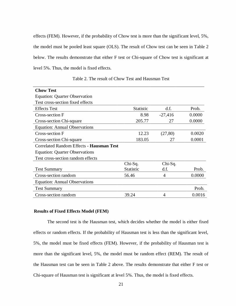
21
effects (FEM). However, if the probability of Chow test is more than the significant level, 5%,
the model must be pooled least square (OLS). The result of Chow test can be seen in Table 2
below. The results demonstrate that either F test or Chi-square of Chow test is significant at
level 5%. Thus, the model is fixed effects.
Table 2. The result of Chow Test and Hausman Test
Chow Test
Equation: Quarter Observation
Test cross-section fixed effects
Effects Test Statistic d.f. Prob.
Cross-section F
8.98 -27,416 0.0000
Cross-section Chi-square 205.77 27 0.0000
Equation: Annual Observations
Cross-section F 12.23 (27,80) 0.0020
Cross-section Chi-square 183.05 27 0.0001
Correlated Random Effects - Hausman Test
Equation: Quarter Observations
Test cross-section random effects
Test Summary
Chi-Sq.
Statistic
Chi-Sq.
d.f. Prob.
Cross-section random 56.46 4 0.0000
Equation: Annual Observations
Test Summary
Prob.
Cross-section random 39.24 4 0.0016
Results of Fixed Effects Model (FEM)
The second test is the Hausman test, which decides whether the model is either fixed
effects or random effects. If the probability of Hausman test is less than the significant level,
5%, the model must be fixed effects (FEM). However, if the probability of Hausman test is
more than the significant level, 5%, the model must be random effect (REM). The result of
the Hausman test can be seen in Table 2 above. The results demonstrate that either F test or
Chi-square of Hausman test is significant at level 5%. Thus, the model is fixed effects.

22
The fixed effects model is the appropriate model for this study. The result of
regression of both quarterly observations and annual observations can be seen in Table 3
below. Sign of the coefficient of earnings before tax and allowance (EBTA), loan provided by
banks to consumer (LOAN), non performing loan (NPL) is positive, but sign of the
coefficient of total assets of banks to measure bank size (SIZE) is negative. Every sign is
proper with the sign illustrated by the theory above (Anandarajana et al., 2007; Kilic et al.,
2010; Alali and Jaggi, 2011).
Based on panel A of Table 3, we can observe quarter data of AIL, EBTA, LOAN,
NPL, and SIZE. Any increase of 117.25% earnings before tax and allowance (EBTA) would
increase the allowance for impairment loss (AIL) by 1%, and every increase of 48.97% non
performing loan (NPL) would increase the AIL by 1%. The increase is significant at level of
5%. Nevertheless, an increase of 2.99% LOAN and a decrease in 18.25% total assets (SIZE)
are not significant at 5%. In panel B we can see annual data of AIL, EBTA, LOAN, NPL, and
SIZE. Any increase of 134.15% EBTA, 419.45% LOAN, and 96.79% NPL would increase
the AIL by 1%, and every decrease of 430.31% SIZE would increase the AIL by 1%. The rise
and decline are significant at 5%. Both quarter and annual observations provide the same sign
for SIZE, that is, negative. This result is in line with theory.
Both panel A and panel B illustrate that the effect of annual earnings before tax and
allowance for impairment loss (134.15%) is bigger than the effect of quarter earnings before
tax and allowance for impairment loss (117.25%). The impact of annual non performing loan
on allowance for impairment loss (96.79%) is also bigger than the impact of quarter non
performing loan on allowance for impairment loss (48.97%).
Table 3. The Result of Panel Least Square Method

23
Panel A. Quarterly Observations
AIL = -0.73 + 1.17EBTA + 0.03LOAN + 0.49NPL - 0.18SIZE
C Log EBTA Log LOAN Log NPL Log SIZE
Coefficient -0.730 1.170 0.030 0.490 -0.180
Std. Error 1.490 0.080 0.090 0.140 0.230
t-Statistic -0.490 15.29** 0.330 3.47** -0.810
Prob. 0.630 0.000 0.740 0.001 0.420
F-Statistic 71.86**
Panel B. Annual
Observations
AIL = -1.288 + 1.341EBTA + 4.195LOAN + 0.968NPL - 4.303SIZE
Coefficient -1.288 1.341 4.195 0.968 -4.303
Std. Error 3.228 0.353 1.400 0.344 1.422
t-Statistic -0.399 3.796** 2.996** 2.813** -3.025
Prob. 0.691 0.000 0.004 0.006 0.003
F-Statistic 15.647** Note: ** Significant at level 5%. Dependent Variable: Log AIL; AIL is the allowance for impairment
loss, EBTA is earnings before tax and allowance, LOAN is total loan, NPL is non performing loans,
and SIZE is total assets to measure bank size.
Results of Classical Assumption Tests
Autocorrelation Test and Test for Heteroskedasticity
To detect serial correlation in least square regression, we use Durbin-Watson d Test.
The Durbin Watson Statistics of both quarter (1.572493) and annual (3.224810) observation
exhibit that there is statistically significant no autocorrelation. To identify heteroskedasticity
problem, we use Glejser’s test. Glejser’s test is conducted by regressing independent variables
to the absolute value of their residuals (Gujarati, 2004). If the effect of all independent
variables (EBTA, LOAN, NPL, SIZE) on their residuals (RESID_QT and RESID_AN) is not
statistically significant at level 5%, there is no heteroskedasticity problem. The result of
regression is shown in Table 4 below. Based on the Table 4 it can be seen that all independent

24
variables (EBTA, LOAN, NPL, and SIZE) of both quarter and annual data statistically do not
affect their residual. This means that there is no heteroscedasticity problem.
Table 4. Heteroscedasticity Test
Panel A. Quarterly Observations
C Log EBTA Log LOAN Log NPL Log SIZE
Coeffcient 0.000 0.000 0.000 0.000 0.000
Std. Error 1.491 0.077 0.090 0.141 0.227
t-Statistic 0.000* 0.000* 0.000* 0.000* 0.000*
Prob. 1.000 1.000 1.000 1.000 1.000
Panel B. Annual
Observations
Coeffcient 0.000 0.000 0.000 0.000 0.000
Std. Error 3.228 0.353 1.400 0.344 1.422
t-Statistic 0.000* 0.000* 0.000* 0.000* 0.000*
Prob. 1.000 1.000 1.000 1.000 1.000 Note: * Not significant at level 5%. Dependent Variable for quarterly observations: RESID_QT and for annual observations: RESID_AN; method: Panel Least Squares; sample: 2008Q1-2011Q4; periods
include: 16; cross section include: 28; total observations for quarterly observations: 448 and for annual
observations: 112.
Hypothesis Test
To test whether managers use the allowance for impairment loss to smooth income,
we use the association between earnings before taxes and allowance (EBTA) and the
allowance for impairment loss (AIL). The empirical research methods demonstrate that to
smooth income, banks increase the level of LLP or AIL when EBTP or EBTA is high and
reduce the level of LLP when EBTP is low. Consequently, a positive coefficient on EBTP
reflects smoothing via LLP (Anandarajana et al., 2007; Kilic et al., 2010; Alali and Jaggi,
2011).

25
The results are exposed in Table 3 above. The correlation between allowance for
impairment loss (AIL) and earnings before tax and allowance (EBTA) of quarter and annual
AIL and EBTA is statistically positive significant (β1=1.172465, prob.= 0.0000; and
β1=1.341460, prob.= 0.0003, respectively). This suggests that banks increase the level of the
allowance when earnings before tax and allowance are high. In addition, banks decrease the
level of the allowance when earnings before tax and allowance are low. This result supports
the empirical conclusions that bank managers use loan loss provision to smooth their income
(Bhat, 1996; Anandarajana et al., 2003, 2007; Kanagaretnam et al., 2007, Borneman, 2010;
Kilic et al., 2010; Alali and Jaggi, 2011). This result supports H1.
The Results of Quarterly Panel Data Regression
Table 5. The Results of Quarterly Panel Data Regression
Variable Coefficient Std. Error t-Statistic Prob.
C -1.501097 0.522268 -2.874186 0.0043
Log EBTA 1.204359 0.085574 14.07393 0.0000
Log LOAN 0.084771 0.089434 0.947863 0.3439
Log NPL 0.439797 0.111004 3.961996 0.0001
Log SIZE -0.148592 0.133083 -1.116534 0.2651
R-squared 0.835034 Mean dependent var 4.599653
Adjusted R-squared 0.822304 S.D. dependent var 1.158450
F-statistic 65.59341 Durbin-Watson stat 1.346425
Prob(F-statistic) 0.000000
Note: Dependent Variable: allowance for impairment loss (AIL); method: Panel Least Squares;
sample: 2008Q1-Q3 – 2011Q1-Q3; periods include: 12; cross section include: 28; total observations:
336.
To identify income smoothing behavior of banks managers in quarterly earnings, we
conduct t-test of quarterly panel data regression of periods: 2008:Q1-Q3 – 20011:Q1-Q3. The
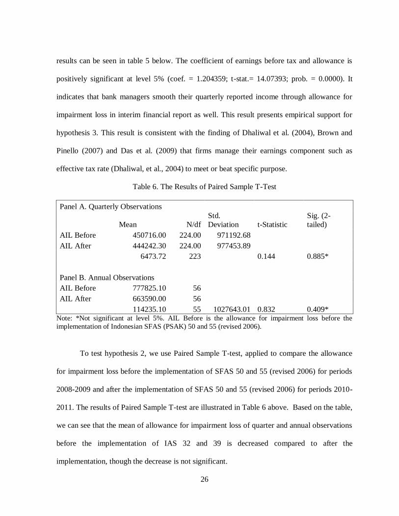
26
results can be seen in table 5 below. The coefficient of earnings before tax and allowance is
positively significant at level 5% (coef. = 1.204359; t-stat.= 14.07393; prob. = 0.0000). It
indicates that bank managers smooth their quarterly reported income through allowance for
impairment loss in interim financial report as well. This result presents empirical support for
hypothesis 3. This result is consistent with the finding of Dhaliwal et al. (2004), Brown and
Pinello (2007) and Das et al. (2009) that firms manage their earnings component such as
effective tax rate (Dhaliwal, et al., 2004) to meet or beat specific purpose.
Table 6. The Results of Paired Sample T-Test
Panel A. Quarterly Observations
Mean N/df
Std.
Deviation t-Statistic
Sig. (2-
tailed)
AIL Before 450716.00 224.00 971192.68
AIL After 444242.30 224.00 977453.89
6473.72 223
0.144 0.885*
Panel B. Annual Observations
AIL Before 777825.10 56
AIL After 663590.00 56
114235.10 55 1027643.01 0.832 0.409* Note: *Not significant at level 5%. AIL Before is the allowance for impairment loss before the
implementation of Indonesian SFAS (PSAK) 50 and 55 (revised 2006).
To test hypothesis 2, we use Paired Sample T-test, applied to compare the allowance
for impairment loss before the implementation of SFAS 50 and 55 (revised 2006) for periods
2008-2009 and after the implementation of SFAS 50 and 55 (revised 2006) for periods 2010-
2011. The results of Paired Sample T-test are illustrated in Table 6 above. Based on the table,
we can see that the mean of allowance for impairment loss of quarter and annual observations
before the implementation of IAS 32 and 39 is decreased compared to after the
implementation, though the decrease is not significant.

27
This insignificant result is caused by several factors. First, commercial banks are
obligated to adopt SFAS 50 and 55 (revised 2006) on January 1st 2010. While the Indonesian
Central Bank permits one year postponement to implement these SFASs, there are several
banks postponed implementing these SFASs until January 1st 2011. We can not release the
banks that not ready yet to apply the SFASs from our sample because banks do not explicitly
affirm this condition in their financial report. Second, research periods used to compare the
effect of the SFASs on earnings management, 2008:I – 2009:IV compared to 2009:I –
2011:IV, are too short, so the effect is not visible yet. The implementation of new accounting
standard statement does not immediately change firms’ financial position. It takes time for
firms to adjust their accounting practice to new accounting standard statements. Perhaps, if
the periods of study were extended until 2015, the significance level would appear. Based on
these results we conclude that this study reject H2.
Conclusion
In this paper we examine earnings management behavior of commercial banks in
Indonesia for periods 2008-2011. We also investigate the ability of new accounting standards
to reduce earnings management of commercial banks in Indonesia. By applying panel time
series cross sectional model, we conclude that commercial bank managers use the allowance
for impairment loss to smooth their earnings, and they also smooth not only their annual
earnings but also quarterly reported earnings. This study also indicate that the implementation
of SFAS 50 and 55 (revised 2006) or IAS 32 and 39 is not significant to reduce the level of
earnings management of public commercial banks in Indonesia.

28
References
Ahmed, A. S., C. Takeda, and S. Thomas, 1999, Bank loan loss provisions: a reexamination
of capital management, earnings management and signaling effects, Journal of
Accounting and Economics 28, 1–25.
Alali, Fatima., and Bikki Jaggi. 2011. Earnings versus Capital Ratios Management: Role of
Bank Types and SFAS 114. Review of Quantitative Finance Accounting 36: 105-132
Anandarajana, Asokan., Iftekhar Hasan, Cornelia McCarthyc. 2007. Use of loan loss
provisions for capital, earnings management and signaling by Australian banks.
Accounting and Finance, 47, p.357–379.
Baltagi, Badi H., 2001. Econometric Analysis of Panel Data. Second Edition. John Willey and
Sons.
Barth, M.E., W.R. Landsman, and M. Lang. 2005. International Accounting Standard and
Accounting Quality. Working paper, Stanford University and University of North
Carolina.
Beatty, Anne L., S. Chamberlain, and J. Magliolo, 1995, Managing financial reports of
commercial banks: the influence of taxes, regulatory capital, and earnings, Journal of
Accounting Research 33, 231–262.
Beatty, Anne L. Bin Ke, and Kathy R. Petroni. 2002. Earnings Management to Avoid
Earnings Declines across Publicly and Privately Held Banks. The Accounting Review,
Vol. 77, No. 3 (Jul., 2002), pp. 547-570.
Bhat, V., 1996, Banks and income smoothing: an empirical analysis, Applied Financial
Economics 6, 505–510.
Bornemann, Sven, Susanne Homölle, Carsten Hubensack, Thomas Kick, and Andreas
Pfingsten. 2009. Determinants for using visible reserves in German banks – an
empirical study. Discussion Paper of Deutsche Bundesbank, Series 2: Banking and
Financial Studies, No 11.
Brewer, Elijah. Liquidity ratios weakened at district banks in 1977. 1980. Economic
Perspective of Federal Reserve Bank of Chicago.
Brown,. and A.S. Pinello, 2007, To What Extent Does the Financial Reporting Process Curb
Earnings Surprise Games? Journal of Accounting Research. Vol 45 (5).
Chang, Ruey-Dang., Wen-Hua Shen., and Chun-Ju Fang. 2008. Discretionary Loan Loss
Provisions And Earnings Management For The Banking Industry. International
Business & Economics Research Journal. Volume 7, Number 3.

29
Clair, Robert T., 1992. Loan Growth and Loan Quality: Some Preliminary Evidence from
Texas Banks. Economic Review - Third Quarter 1992.
Collins, J., D. Shackelford, and J. Wahlen, 1995, Bank differences in the coordination of
regulatory capital, earnings and taxes. Journal of Accounting Research 33, 263–292
Das, Somnath, Pervin K. Shroff, and Haiwen Zhang. 2009. Quarterly Eamings Patterns and
Eamings Management. Contemporary Accounting Research Vol. 26 No. 3. pp. 797-
831.
Degeorge, Francois, Jayendu Patel, Richard Zeckhauser. 1999. Earnings Management to
Exceed Thresholds. The Journal of Business, Vol. 72, No. 1, pp. 1-33.
Demski, J. S. 2004. Endogenous Expectations. The Accounting Review 79. Pp. 513-539.
Dhaliwal, D., C. Gleason, and L. Mills. 2004. Last chance earnings management: Using the
tax expense to meet analysts' forecasts. Contemporary Accounting Research 21 (2). Pp.
431-59.
Eng, Li Li., Sandeep Nabar. 2007. Loan Loss Provisions by Banks in Hong Kong, Malaysia,
and Singapore. Journal of International Financial Management and Accounting, Vol
18, No. 1.
Ewert, Ralf., Alfred Wagenhofer. 2005. Economic Effects of Tightening Accounting
Standards to Restrict Earnings Management. The Accounting Review. Vol. 80. No. 4.
Pp. 1101-1124.
Fonseca, Ana Rosa and Gonzales Fransisco. 2008. Cross-country determinants of bank
income smoothing by managing loan-loss provisions. Journal of Banking & Finance;
Feb2008, Vol. 32 Issue 2, p217-228, 12p.
Fudenberg, Drew, and Jean Tirole. 1995. A theory of income and dividend smoothing based
on incumbency rents. Journal of Political Economy 103, no. 1: 75-93.
Greenawalt, M., and J. Sinkey Jr, 1988, Bank loan loss provisions and the income smoothing
hypothesis: an empirical analysis, 1976–84, Journal of Financial Services Research 1,
301–318.
Gujarati, D., 2004. Basic Econometric. Mc-Grawhill, New York.
Gujarati, Damodar N., and Dawn C. Porter. 2009. Basic Econometrics. Fifth Edition.
McGraw – Hill/Irwin.

30
Gujarathi, Mahendra R. and Robert E. Hoskin. 1992. Evidence of Earnings Management by
the Early Adopters of SFAS 96. Accounting Horizons. Vol. 6. Issue 4. pp. 18-31.
Hasan, Iftekhar, and Larry D. Wall. 2003. Determinants of the loan loss allowance: some
cross-country comparisons. Bank of Finland Discussion Papers.
Hsiao, Cheng. 2003. Analysis of Panel Data. Second Edition. Cambridge University Press.
Haw, In-Mu., Daqing Qi, Donghui Wu, Woody Wu., 2005. Market Consequences of Earnings
Management in Response to Security Regulations in China. Contemporary Accounting
Research Vol. 22 No. 1. pp. 95-140.
Healy, Paul M. 1985. The effect of bonus schemes on accounting decisions. Journal of
Accounting and Economics 7: 85-107.
Healy, Paul M., and James M. Wahlen. 1999. A Review of the Earnings Management
Literature and Its Implications for Standard Setting. Accounting Horizons, Vol. 13 No.
4. pp. 365-383.
Hopwood, W.S., J.C. Mckeown, and P. Newbold. 1982. The Additional Information Content
of Quarterly Earnings Reports: Intertemporal Disaggregation. Journal of Accounting
Research, Vol. 20. No. 2. Pt. I.
Kanagaretnam, Kinidaran Giri, Robert Mathieu, Gerald J. Lobo. 2003. Managerial Incentives
for Income Smoothing Through Bank Loan Loss Provision. Review of Quantitative
Finance and Accounting. Vol. 20 January 2003.
Kanagaretnam, K., G. Lobo, and D. Yang. 2004. Joint tests of signaling and income
smoothing through Bank Loan Loss Provisions. Contemporary Accounting Research
21 (4): 843-884.
Kilic, Emre., Gerald J. Lobo, Tharindra Ranasinghe, K. (Shiva) Sivaramakrishnan. 2010. The
Impact of SFAS 133 on Income Smoothing by Banks through Loan Loss Provisions.
Working Paper, C. T. Bauer College of Business University of Houston.
Kim, M., and W. Kross, 1998, The impact of the 1989 change in bank capital standards on
loan loss provisions and loan write-offs. Journal of Accounting and Economics 25,
69–100.
Kwag, Seung-Woog, and Kenneth Small. 2007. The Impact of Regulation Fair Disclosure on
Earnings Management and Analyst Forecast Bias. Journal of Economics and Finance.
Vol. 31, No. 1. Spring 2007. 87.

31
Liang, Pierre Jinghong. 2004. Equilibrium Earnings Management, Incentive Contracts, and
Accounting Standards. Contemporary Accounting Research Vol. 21 No. 3 pp. 685-717.
Liu, C., and S. Ryan, 1995, The effect of bank loan portfolio composition on the market
reaction to and anticipation of loan loss provisions, Journal of Accounting Research
33, 77–94.
Liu, C., and S. Ryan. 2006. Income smoothing over the business cycle: Changes in banks'
coordinated management of provisions for loan losses and loan charge-offs from the
pre-1990 bust to the 1990s boom. The Accounting Review 81 (2): 421-441.
Liu, C., S. Ryan, and J. Wahlen, 1997, Differential valuation implications of loan loss
provisions across banks and fiscal agents, The Accounting Review 72, 133–146.
Lobo, Gerald J., Dong-Hoon Yang. 2001. Bank Manager’ Heterogeneous Decisions on
Discretionary Loan Loss Provisions. Review of Quantitative Finance and Accounting.
16:223-250.
Ma, C. K., 1988, Loan loss reserve and income smoothing: the experience in the U.S. banking
industry, Journal of Business Finance and Accounting 15, 487–497.
Maddala, G.S., and Kajal Lahiri. 2009. Introduction to Econometrics. Fourth Edition. John
Wiley and Sons Ltd.
Montgomery, L., 1998, Recent developments affecting depository institutions, FDIC Banking
Review 11, 26–34.
Moyer, S. E., 1990, Capital adequacy ratio regulations and accounting choices in commercial
banks, Journal of Accounting and Economics 13, 123–154.
Oosterbosch, Renick van. 2009. Earnings Management in the Banking Industry: The
consequences of IFRS implementation on discretionary use of loan loss provisions.
Master thesis of the master Accounting Auditing & Control at Erasmus University
Rotterdam.
Pinho, Paulo Soares de., and Nuno Carvalho Martins. 2009. Determinants of Portuguese
Bank’s Provisioning Policies: Discretionary Behavior of Generic and Specific
Allowances. Journal of Money, Investment and Banking ISSN 1450-288X Issue 10
(2009) © EuroJournals Publishing, Inc.
Rivard, Richard, Eugenebland, and Gay B. Hatfieldmorris. 2003. Income Smoothing
Behavior of U.S Banks under Revised International Capital Requirements. IAER 9 No.
4.
32
Smith, James A. and Zabihollah Razaee. 1995. Earnings Management by the Early Adopters
of SFAS No. 106. International Advance in Economic Research. Vol 1. No. 4.
Stefanescu, Monica. 2006. The Effect of SFAS 144 on Managers’ Income Smoothing
Behavior. Working Paper, Smeal College of Business, the Pennsylvania State
University.
Wahlen, J. 1994. The nature of information in commercial bank loan loss disclosures. The
Accounting Review 69 (3): 455-478.
Wetmore, J. L., and J. R. Brick, 1994, Loan loss provisions of commercial banks and
adequate disclosure: a note, Journal of Economics and Business 46, 299–305.
Zhou, Haiyan., Yan Xiong., and Gouranga Ganguli. 2009. Does the Adoption of International
Financial Reporting Standards Restrain Earnings Management? Evidence from an
Emerging Market. Academy of Accounting & Financial Studies Journal. Supplement,
Vol. 13, p43-56, 14p, 6.
Moses, O. Douglas. 1987. Income Smoothing and Incentives: Empirical Tests Using
Accounting Changes. The Accounting Review. Vol. 62. No.2. pp. 358-377.
Rudra, Titas, and CA. Dipanjan Bhattacharjee. 2012. Does IFRS Influence Earnings
Management? Evidence from India. Journal of Management Research Vol. 4, No. 1:
E7.