cost functions in optical burst-switched networksdoras.dcu.ie/17996/1/bartlomiej_klusek.pdf · cost...
TRANSCRIPT
Cost functions in Optical
Burst-Switched networks
Bartlomiej Klusek
under the supervision of
Dr John Murphy and Dr Liam Barry
A thesis submitted m June 2006 for the degree of Doctor of Philosophy m
the School of Electronic Engineering, Dublin City University
I hereby certify that this material, which
I now submit for assessment on the pro
gramme of study leading to the award
of Doctor of Philosophy is entirely my
own work and has not been taken from
the work of others save and to the ex
tent that such work has been cited and ac
knowledged within the text of my work
Signed 5
ID No 50162616
11th of June, 2006

To Ahqa
Abstract
Optical Burst Switching (OBS) is a new paradigm for an all-optical In
ternet It combines the best features of Optical Circuit Switching (OCS)
and Optical Packet Switching (OPS) while avoidmg the mam prob
lems associated with those networks Namely, it offers good granular
ity, but its hardware requirements are lower than those of OPS
In a backbone network, low loss ratio is of particular importance Also,
to meet varying user requirements, it should support multiple classes
of service In Optical Burst-Switched networks both these goals are
closely related to the way bursts are arranged in channels Unlike the
case of circuit switching, scheduling decisions affect the loss probabil
ity of future bursts
This thesis proposes the idea of a cost function The cost function is
used to ]udge the quality of a burst arrangement and estimate the
probability that this burst will interfere with future bursts Two ap
plications of the cost fu n c tio n are proposed A scheduling algorithm
uses the value of the cost function to optimize the alignment of the
new burst with other bursts in a channel, thus minimising the loss ra
tio A cost-based burst droppmg algorithm, that can be used as a part
of a Quality of Service scheme, drops only those bursts, for which the
cost function value indicates that are most likely to cause a contention
Simulation results, performed using a custom-made OBS extension to
the ns-2 simulator, show that the cost-based algorithms improve net
work performance
IV
List of publications
• Bartlomiej Klusek, John Murphy and Liam Barry, "Cost-based burst drop
ping strategy m Optical Burst Switching networks", In Proceedings of IEEE
7th International Conference on Transparent Optical Netwoiks, July 2005
• Bartlomiej Klusek, John Murphy and Liam Barry, "New Fiber Delay Lme
Usage Strategy in Optical Burst Switching Node," in Proceedings oflASTED
Networks and Communication Systems, Apr 2005
• Bartlomiej Klusek, John Murphy and Liam Barry, "Traffic sources for Optical
Burst Switching simulations," in Proceedings ofSPIE OPTO Ireland, Apr 2005
• Bartlomiej Klusek, John Murphy and Philip Perry, "Cost-based wavelength
allocation algorithms m optical burst switching networks," in Proceedings of
Asia-Pacific Optical Communications, Nov 2004
• Dawid Nowak and Bartlomiej Klusek, "Analysis of Waveband Connect
ing Probability in Hybrid Optical Networks," in Proceedings of 2nd IFIP-TC6
International Conference on Optical Communications and Networks, Oct 2003
• Dawid Nowak, Bartlomiej Klusek, and Tommy Curran, "New Method for
Calculating Probability of Waveband Connection in All Optical Networks,"
in Proceedings oflEI/IEE Telecommunications System Research Symposium, May
2003
• Bartlomiej Klusek, Dawid Nowak, and Tommy Curran, "Wavelength As
signment Algorithms m an OBS Node," in Proceedings oflEI/IEE Telecommu
nications System Research Symposium, May 2003
Contents
1 Introduction 1
11 Thesis contribution 4
1 2 Thesis overview 5
2 Optical Burst Switching 72 1 Burst switching protocols 8
2 11 Just-In-Time (JIT) 8
2 1 2 Horizon 10
2 1 3 Just-Enough-Time (JET) 10
2 2 Burst assembly 11
2 21 Time and size - based algorithms 12
2 2 2 Adaptive algorithms 14
2 2 3 Composite burst assembly 15
2 2 4 Predictive burst assembly 15
2 3 Node architecture 17
2 31 Broadcast-and-Select (BAS) 19
2 3 2 Tune-and-Select (TAS) 20
2 3 3 Wavelength grating router (WGR) based node 21
2 4 Scheduling algorithms 22
2 5 Time Sliced Optical Burst Switching (TSOBS) 23
2 6 OBS testbeds 23
2 7 Summary 26
VI
Contents
3 Scheduling algorithms and Quality of Service 273 1 Scheduling algorithms 27
3 1 1 Legacy scheduling algorithms 29
3 1 2 Per-burst schedulmg algorithms 29
3 1 3 Batch scheduling algorithms 34
3 1 4 Burst rescheduling algorithms 36
3 2 Quality of service 38
3 21 Offset-based QoS 38
3 2 2 Composite burst assembly 39
3 2 3 Intentional burst dropping 40
3 2 4 Assured Horizon 41
3 2 5 Preferred wavelength sets 42
3 2 6 Preemptive wavelength reservation protocol (PWRP) 42
3 2 7 Probabilistic Preemptive scheme (PP) 43
3 2 8 Partially Preemptive Burst Scheduling with Proportional Dif
ferentiation 44
3 2 9 DiffServ over Optical Burst Switching (DS-OBS) 45
3 3 Summary 46
4 Cost functions 47
41 Motivation 47
4 2 Definition 48
4 3 Cost function formulas 48
4 4 Applications of a cost function 56
4 41 Scheduling algorithms 56
4 4 2 FDL management 58
4 4 3 Quality of Service - selective burst dropping 59
4 5 Summary 60
V ll
Contents
5 Simulator 625 1 Existing OBS simulation programs 62
5 2 Stand-alone simulator vs extension to an existing simulator 63
5 3 Ns-2 simulator 63
5 4 OBS extension to ns-2 simulator 64
5 41 OBS object 64
5 4 2 OBSCoreNode 65
5 4 3 OBSEdgeNode 65
5 4 4 OpticalLink 66
5 4 5 BurstAssembler 66
5 4 6 BurstLogger 67
5 5 Traffic sources 69
5 51 BurstAssembler/Exponential 69
5 5 2 BurstAssembler/Generator 70
5 5 3 BurstAssembler/EnvelopeGenera tor 71
5 5 4 Generators class 72
5 6 Scheduling algorithms 73
5 7 Burst dropping 74
5 8 Simulator validation 75
5 9 Routing 76
5 91 IP routmg 76
5 9 2 OBS routing 77
5 10 Example simulations 77
5 10 1 Network with burst assemblers 78
5 10 2 Network with burst generators 82
5 11 Summary 87
6 Results and discussion of cost-based scheduling 8861 Introduction 88
V lll
Contents
6 2 Single node scenario 91
6 21 Basic simulation 91
6 2 2 Effects of traffic type 98
6 2 3 Effects of offset time range 103
6 2 4 Effects of FDL length 106
6 25 Effects of FDL bank size 110
6 3 Network examples 113
6 31 Ring network 113
6 3 2 US network 116
6 3 3 Pan-European network 122
6 4 Summary 128
7 Results and discussion of cost-based burst dropping 13071 Introduction 130
7 2 Single node 132
7 21 Basic simulation 132
7 2 2 Effect of traffic type 133
7 2 3 Effect of offset time range 135
7 3 Network examples 136
7 31 Ring network 136
7 3 2 Random networks 138
7 4 Summary 142
8 Conclusions 1438 1 Future work 146
Bibliography 147
A Simulation scripts 159A 1 Cost-based scheduling 159
IX
Contents
A 2 Burst dropping 165
A 3 Burst dropping, complex topologies 171
List of Figures
1 1 Evolution of optical networks 2
2 1 Just-In-Time (JIT) protocol 9
2 2 Just-Enough-Time (JET) protocol 10
2 3 Structure of a burst assembler 11
2 4 Predictive burst assembly 16
2 5 Architecture of a WDM node 18
2 6 Architecture of a generic OBS node 18
2 7 2D MEMS switch 19
2 8 Broadcast-And-Select (BAS) node architecture 20
2 9 Tune-And-Select (TAS) node architecture 21
2 10 Wavelength grating router based node 22
211 ATDnefOptical Time Slot Interchanger 24
2 12 ATDnet OBS testbed configuration 25
3 1 Different scheduling algorithms 28
3 2 Horizon scheduling algorithm 30
3 3 Last Available Unused Channel with Void Filling (LAUC-VF) 31
3 4 Minimum Ending Void (Min-EV) 32
3 5 Overlapping bursts arrived 33
3 6 Reduced overlap 33
3 7 Waitmg-Queumg-Scheduling algorithm 35
3 8 Burst rescheduling 37
3 9 Tail dropping technique 40
XI
LIST OF FIGURES
3 10 PWRP algorithm 43
311 Probabilistic Preemptive scheme 44
312 Classification of scheduling algorithms 46
41 A single-channel OBS system 49
4 2 Burst transmission process 50
4 3 Contention range m the first period 52
4 4 Contention range in the second period 53
4 5 Graphical representation of contention probability 54
4 6 Cost-based scheduling 58
4 7 Structure of a generic burst dropper 59
5 1 Structure of an OBSCoreNode 64
5 2 Structure of an OBSEdgeNode 66
5 3 Structure of an OpticdLink 66
5 4 An envelope generator 72
5 5 Measured and calculated burst loss ratios 76
5 6 PseudoLinks withing an OBS network 77
5 7 Example network topology 78
5 8 Network with burst assemblers 82
6 1 Example loss vs FDL price graph 90
6 2 Example FDL usage histograms 90
6 3 Smgle-node network topology 92
6 4 Traffic loss vs FDL price, 0 5 link load 93
6 5 Traffic loss vs FDL price, 0 75 lmk load 93
6 6 Traffic loss vs FDL price, 0 93 link load 94
6 7 FDL usage histograms, linear FDL pricing, 0 5 link load 95
6 8 FDL usage histograms, linear FDL pricing, 0 75 lmk load 95
6 9 FDL usage histograms, linear FDL pricing, 0 93 lmk load 96
xu
LIST OF FIGURES
6 10 Burst loss probability for the cost-based algorithm and LAUC-VF
as a function of link load 97
6 11 FDL usage histograms for the cost-based algorithm and LAUC-VF 97
6 12 Traffic loss vs FDL price, 0 5 lmk load, variable burst length 98
6 13 Traffic loss vs FDL price, 0 75 lmk load, variable burst length 99
6 14 Traffic loss vs FDL price, 0 93 lmk load, variable burst length 99
6 15 Burst loss probability as a function of lmk load, variable burst length 100
6 16 Traffic loss vs FDL price, 0 5 lmk load, assembled traffic 101
617 Traffic loss vs FDL price, 0 75 lmk load, assembled traffic 102
618 Traffic loss vs FDL price, 0 9 lmk load, assembled traffic 102
6 19 Burst loss probability as a function of lmk load, assembled traffic 103
6 20 Burst loss probability as a function of lmk load, offset time range
equal to one burst length 104
6 21 Burst loss probability as a function of lmk load, offset time range
equal to three burst lengths 104
6 22 Burst loss probability as a function of lmk load, offset time range
equal to six burst lengths 105
6 23 Burst loss probability as a function of lmk load, offset time range
equal to fifteen burst lengths 105
6 24 Burst loss probability as a function of offset time range, lmk
load 0 75 106
6 25 Burst loss vs FDL price, 0 75 link load, FDL length 0 1 of burst
length 107
6 26 Burst loss vs FDL price, 0 75 lmk load, FDL length 0 3 of burst
length 108
6 27 Burst loss vs FDL price, 0 75 link load, FDL length equal to burst
length 108
6 28 Burst loss vs FDL price, 0 75 lmk load, FDL length equal to three
burst lengths 109
x i u
LIST OF FIGURES
6 29 Burst loss vs FDL length, 0 75 link load 109
6 30 Burst loss vs link load, different FDL lengths 110
6 31 Burst loss vs FDL bank size, 0 75 link load 112
6 32 FDL usage histograms, 10 FDL channels, 0 75 link load 112
6 33 FDL usage histograms, 40 FDL channels, 0 75 link load 113
6 34 The ring network topology 114
6 35 Burst loss vs FDL bank size, 0 72 link load, ring network 115
6 36 FDL usage histograms, 9 FDL channels, ring network 115
6 37 US network topology 116
6 38 Burst loss probability m subsequent iterations, US network 118
6 39 FDL usage histograms, US network, cost-based algorithm,
iteration 1 119
6 40 FDL usage histograms, US network, cost-based algorithm,
iteration 2 119
6 41 FDL usage histograms, US network, cost-based algorithm,
iteration 3 120
6 42 FDL usage histograms, US network, cost-based algorithm,
iteration 4 120
6 43 FDL usage histograms, US network, cost-based algorithm,
iteration 5 121
6 44 Burst loss vs network load, US network 121
6 45 Pan-European network topology 123
6 46 Burst loss probability in subsequent iterations, European network 123
6 47 FDL usage histograms, European network, cost-based algorithm,
iteration 1 126
6 48 FDL usage histograms, European network, cost-based algorithm,
iteration 2 126
6 49 FDL usage histograms, European network, cost-based algorithm,
iteration 3 127
xiv
LIST OF FIGURES
6 50 FDL usage histograms, European network, cost-based algorithm,
iteration 4 127
6 51 Burst loss probability as a function of load, European network 128
7 1 Example low priority vs high priority loss ratio diagrams 131
7 2 Burst droppmg in a single link 132
7 3 Low priority vs high priority loss ratio, 0 7 link load 133
7 4 Low priority vs high priority loss ratio, 0 8 link load 134
7 5 Low priority vs high priority loss ratio, 0 9 link load 134
7 6 Low priority vs high priority loss ratio, 0 8 lmk load, variable
burst length 135
7 7 Low priority vs high priority loss ratio, 0 8 lmk load, assembled
traffic 136
7 8 Low priority vs high priority loss ratio, 0 8 lmk load, offset time
range 1 burst length 137
7 9 Low priority vs high priority loss ratio, 0 8 link load, offset time
range 5 burst lengths 137
7 10 Low priority vs high priority loss ratio, 0 8 link load, offset time
range 15 burst lengths 138
7 11 Low priority vs high priority loss ratio, 0 7 lmk load, rmg network 139
7 12 Low priority vs high priority loss ratio, 0 9 link load, rmg network 139
7 13 Low priority vs high priority loss ratio, random network 0 140
7 14 Low priority vs high priority loss ratio, random network 1 141
7 15 Low priority vs high priority loss ratio, random network 2 141
xv
List of acronyms
AAP Adaptive Assembly Period
ABR Aggressive Burst Rescheduling Algorithm
ATM Asynchronous Transfer Mode
AWGM Arrayed Waveguide Grating Multiplexer
BAS Broadcast- And-Select
BORA Burst Overlap Reduction Algorithm
DARPA Defense Advanced Research Projects Agency
DIA Defense Intelligence Agency
D-PWS Dynamic Preferred Wavelength Sets
DS-OBS DiffServ over OBS
DWDM Dense Wavelength Division Multiplexing
FAP Fixed Assembly Period
FDL Fiber Delay Line
GMPLS Generalized Multiprotocol Label Switching
IETF Internet Engineering Task Force
IP Internet Protocol
JET J ust-Enough-Time
JIT Just-In-Time
JITPAC Just-m-Time Protocol Acceleration Circuit
LAUC-VF Last Available Unused Channel with Void Filling
LTS Laboratory for Telecommunications Science (NSA)
Min-EV Mmimum Ending Void
Mm-SV Minimum Starting Void
xvi
List of acronyms
MSSIS Maximum Stable-Set Interval Schedulmg Algorithm
NRL Naval Research Laboratory
OBS Optical Burst Switching
OCS Optical Circuit Switching
ODBR On-Demand Burst Rescheduling Algorithm
OEO Optical-Electrical-Optical
OPS Optical Packet Switching
OTSI Optical Time Slot Interchanger
OWns Optical WDM Network Simulator
PLC Planar Lightwave Circuit
PP Probabilistic Preemptive scheme
PWA Priority-based Wavelength Assignment
PWRP Preemptive Wavelength Reservation Protocol
QoS Quality of Service
SDH Synchronous Digital Hierarchy
SOA Semiconductor Optical Amplifier
SONET Synchronous Optical Network
TAG Tell-And-Go
TAS Tune-And-Select
TCP Transmission Control Protocol
TSOBS Time Sliced OBS
VoIP Voice over IP
WDM Wavelength Division Multiplexing
WGR Wavelength grating router
WSQ Waitmg-Queuing-Schedulmg
x v n
Chapter 1
Introduction
The history of optical communication is probably as long as history of humanity
and possibly longer. When two humans (or apes) needed to exchange some infor
mation while being out of earshot of each other, they gestured. By doing so, they
formed a primitive light-based communication circuit. Their source of light was
almost certainly the sun. It was modulated by the transmitting person's hands,
propagated in the free space and was finally received by the other person's eye.
Millenia later, the development of laser and optical fiber became the enabling
technology for high-speed telecommunications. Without it, the information soci
ety of today would not be possible.
The first widely deployed optical networks were based on optical point-to-
point links and electronic routers, with all multiplexing being done in the electri
cal domain. This SONET/SDH based architecture was inherited from telephony
networks, and is well suited for its original purposes, i.e. carrying voice traffic.
Rapid expansion of the Internet brought several important changes, however.
The most obvious one is an ever-increasing demand for bandwidth. According
to [1J, for 18 years the data traffic doubled every twelve months. Since 1997,
the rate of increase has increased, and today's networks have to cope with traffic
doubling every six months.
The bandwidth offered by an optical fiber is enormous, several orders of mag
nitude bigger than this of twisted pair or coaxial cable. Although not even close
to utilizing the theoretical capabilities, the introduction of wavelength division mul
tiplexing (WDM) made it apparent that the limiting factor would be not the trans
mission, but switching. The clcctronic routers arc the bottlenecks of ftrbt gen
1
Chapter 1 Introduction
o ( Packct Switching
o CBurst Switching
( Meshed networks
cRing networks
( Point-to Point WDM links
time
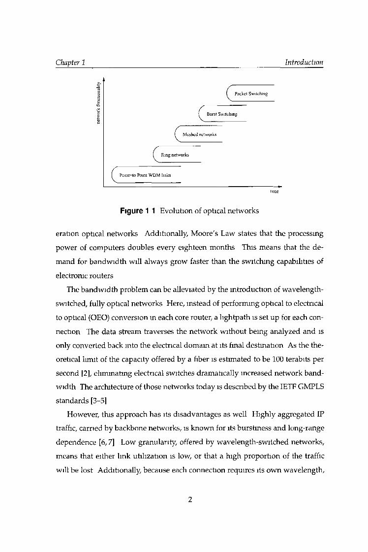
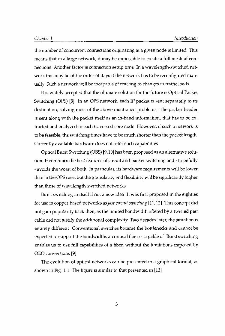
Figure 1 1 Evolution of optical networks
eration optical networks Additionally, Moore's Law states that the processing
power of computers doubles every eighteen months This means that the de
mand for bandwidth will always grow faster than the switchmg capabilities of
electronic routers
The bandwidth problem can be alleviated by the introduction of wavelength-
switched, fully optical networks Here, instead of performmg optical to electrical
to optical (OEO) conversion in each core router, a lightpath is set up for each con
nection The data stream traverses the network without being analyzed and is
only converted back mto the electrical domam at its final destmation As the the
oretical limit of the capacity offered by a fiber is estimated to be 100 terabits per
second [2], eliminating electrical switches dramatically increased network band
width The architecture of those networks today is described by the IETF GMPLS
standards [3-5]
However, this approach has its disadvantages as well Highly aggregated IP
traffic, carried by backbone networks, is known for its burstmess and long-range
dependence [6,7] Low granularity, offered by wavelength-switched networks,
means that either link utilization is low, or that a high proportion of the traffic
will be lost Additionally, because each connection requires its own wavelength,
2
Chapter 1 Introduction
the number of concurrent connections originating at a given node is limited This
means that in a large network, it may be impossible to create a full mesh of con
nections Another factor is connection setup time In a wavelength-switched net
work this may be of the order of days if the network has to be reconfigured man
ually Such a network will be mcapable of reactmg to changes m traffic loads
It is widely accepted that the ultimate solution for the future is Optical Packet
Switchmg (OPS) [8] In an OPS network, each IP packet is sent separately to its
destination, solvmg most of the above mentioned problems The packer header
is sent along with the packet itself as an m-band information, that has to be ex
tracted and analyzed m each traversed core node However, if such a network is
to be feasible, the switching times have to be much shorter than the packet length
Currently available hardware does not offer such capabilities
Optical Burst Switching (OBS) [9,10] has been proposed as an alternative solu
tion It combines the best features of circuit and packet switchmg and - hopefully
- avoids the worst of both In particular, its hardware requirements will be lower
than m the OPS case, but the granularity and flexibility will be significantly higher
than those of wavelength-switched networks
Burst switchmg in itself if not a new idea It was first proposed m the eighties
for use m copper-based networks as fast circuit switching [11,12] This concept did
not gam popularity back then, as the limited bandwidth offered by a twisted pair
cable did not justify the additional complexity Two decades later, the situation is
entirely different Conventional switches became the bottlenecks and cannot be
expected to support the band widths an optical fiber is capable of Burst switchmg
enables us to use full capabilities of a fiber, without the limitations imposed by
OEO conversions [9]
The evolution of optical networks can be presented m a graphical format, as
shown in Fig 11 The figure is similar to that presented in [13]
3
Chapter 1 Introduction
1.1 Thesis contribution
In Optical Burst Switching networks the arrangement of bursts within a channel
is an important issue Manipulating it can affect the overall burst loss probability
Unfortunately, the 'quality' of burst arrangement is diffcult to describe in a
numerical way This thesis attempts to achieve this goal and describe its applica
tions
• Cost function The mam contribution of this thesis is the idea of a cost func
tion Cost function value is expected to be an indicator of how likely is a
given burst to cause contention m future Therefore, cost function can be
used to judge how well a burst is aligned with other bursts in a channel and
to asses suitability of a particular channel for a particular burst
• Soft decision making Most schedulmg algorithms and contention resolution
mechanisms use hard decisions This thesis demonstrates that the decision
whether to use a certain resource or not can be made m a soft way, based on
the value of a cost function
• Fiber Delay Line (FDL) usage algorithm FDLs can be used to reduce the burst
loss ratio This thesis shows how the idea of a cost function can be used to
design a schedulmg algorithm in a FDL-equipped node Use of the addi
tional information, provided by a cost function, allows us to prevent con
tention, instead of resolving it Also, the cost-based algorithm allows us to
match the needs of the node with the size of the available FDL-bank m an
optimal way In effect, the overall burst loss ratio is minimized
• An early dropping algorithm A cost-based burst dropping algorithm is pre
sented This algorithm can be used as a part of Quality of Service scheme,
and allows us to ensure good QoS parameters for high-priority classes while
dropping a minimal amount of low-prionty traffic Alternatively, for a given
4
Chapter 1 Introduction
amount of low-pnority traffic to be dropped, the burst loss ratio m the high-
pnonty class can be minimized
• Simulation tool The last contribution is an OBS extension to the ns-2 simu
lator The efficient and robust underlymg ns-2 engine and its two-language
architecture, coupled with an extensive set of OBS classes created a power
ful simulation tool
1.2 Thesis overview
The rest of this thesis is organized as follows
• Chapter 2 This chapter introduces the basic idea of Optical Burst Switch
ing In particular, it discusses the burst switching and burst assembly algo
rithms
• Chapter 3 In the first part of this chapter schedulmg algorithms used m
Optical Burst Switching are presented The significance of optimal burst
schedulmg is emphasized and several existing schedulmg algorithms are
described The rest of this chapter deal withs ensuring Quality of Service
(QoS) in Optical Burst Switching networks
• Chapter 4 This chapter describes the idea of a cost function along with theo
retical analysis, its proposed formula and possible applications
• Chapter 5 All the simulations described m this thesis were performed using
a custom-built OBS extension to the ns-2 simulator This chapter describes
this extension, its mternal architecture and usage
• Chapter 6 The performance of cost-based schedulmg algorithm m Optical
Burst-Switched networks was tested m several simulations Results of these
simulations are presented and discussed here
5

• Chapter 7 In this chapter the simulation results concerning the cost-based
burst droppmg algorithm are presented and discussed This and two previ
ous chapters form the core of this thesis
• Chapter 8 In this chapter final conclusions are presented
Chapter 1 Introduction
6
Chapter 2
Optical Burst Switching
For a fully transparent optical network to work efficiently without ultra-fast hard
ware, the basic data unit has to be significantly larger that IP packets. Thus, in
coming packets are assembled into bigger entities, called bursts, at the edge node.
While it is usually assumed that bursts will consist of IP packets, an OBS net
work can carry any type of data. For example, ATM cells can be assembled into
bursts. Even analog data can be carried by an OBS network. For simplicity, in the
rest of this thesis, only IP packets will be considered.
An important feature of OBS networks is that control information is separated
from the payload. The control packet is sent ahead of the actual data, using a
different channel. When received by a core node it it converted to the electrical
domain, analyzed and sent to the next node. At each stage a routing decision is
made (if necessary) and a connection is set up. The data burst is then sent by the
edge node without waiting for any acknowledgment. This one-way reservation
protocol is similar to tell-and-go (TAG) [14,15]. Several dedicated OBS protocols
have been designed; their details will be discussed later in this chapter.
The time difference between sending the control packet and the data burst
is called offset time. It is necessary to allow the intermediate nodes to receive
the control packet, prepare a lightpath for the incoming burst and transmit the
control packet to the next node. It is possible to eliminate offset time if at each
node data bursts are delayed in a Fiber Delay Line (FDL) while the control packet
is being analyzed and the connection is being set up.
The data burst traverses the entire network in optical domain. Only at the
destination node is it converted to the electrical domain. It is then disassembled,
7
Chapter 2 Optical Burst Switching
and all the IP packets are sent to their respective destinations On the other hand,
the control packet has to be converted to electrical domain at each core node
However, as it is significantly smaller than the data burst, it can be transmitted at
a much lower bitrate, allowing use of relatively cheap hardware
2.1 Burst switching protocols
In circuit-switched networks, the path is only considered complete after the ini
tiating station has received positive acknowledgment, and no data can be sent
before this happens The resultmg delay is of little consequence, if the average
length of connection is much greater than the required set-up time
Optical bursts, while larger than packets, are still relatively small, and waitmg
for a positive acknowledgment would be inefficient Therefore, other switchmg
protocols had to be developed
2 1.1 Just-In-Time (JIT)
The idea of Just-In-Time switchmg was proposed by Mills in his HIGHBALL
project [16] He used the analogy of trains leaving a station, without setting all
the switches across the country at this moment Instead, the switches are set as
the train approaches This idea can be adapted to optical burst switchmg [17]
When a burst is ready to be sent, the originating node sends the control packet
with a SETUP message first As it traverses the network, at each core node band
width is reserved for the incoming burst Depending on the version of the proto
col, the reservation starts either immediately after the control packet is received
(explicit setup), or at the expected arrival time of burst (estimated setup) The lat
ter option is more efficient, but also more complicated After the burst has been
transmitted, the originating node sends a RELEASE message, lettmg the down
stream nodes know that the transmission has ended and the lightpath can be torn
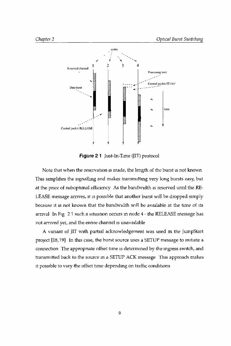
down The reservation process is shown in Fig 2 1
8
Chapter 2 Optical Burst Switching
nodes
A
Reserved channel
Data burst
Control packet RELEASE
Processing time
Control packct SETUP
time
Figure 2 1 Just-In-Time (JIT) protocol
Note that when the reservation is made, the length of the burst is not known
This simplifies the signalling and makes transmitting very long bursts easy, but
at the price of suboptimal efficiency As the bandwidth is reserved until the RE
LEASE message arrives, it is possible that another burst will be dropped simply
because it is not known that the bandwidth will be available at the time of its
arrival In Fig 2 1 such a situation occurs m node 4 - the RELEASE message has
not arrived yet, and the entire channel is unavailable
A variant of JIT with partial acknowledgement was used m the JumpStart
project [18,19] In this case, the burst source uses a SETUP message to initiate a
connection The appropriate offset time is determmed by the ingress switch, and
transmitted back to the source in a SETUP ACK message This approach makes
it possible to vary the offset time depending on traffic conditions
9
Chapter 2 Optical Burst Switching
nodes
2 3 4
Control Packet
Data b u rs t
I I I
Processing time
Itime
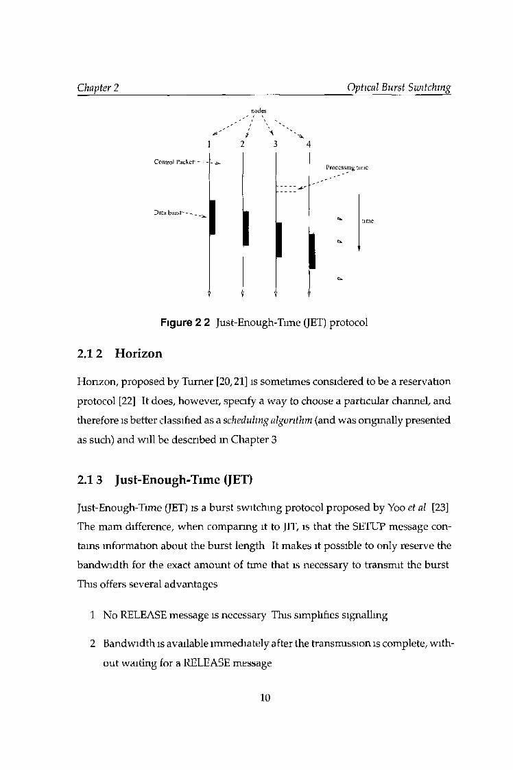
Figure 2 2 Just-Enough-Time (JET) protocol
2.12 Horizon
Horizon, proposed by Turner [20,21] is sometimes considered to be a reservation
protocol [22] It does, however, specify a way to choose a particular channel, and
therefore is better classified as a scheduling algorithm (and was originally presented
as such) and will be described in Chapter 3
2.1 3 Just-Enough-Time (JET)
Just-Enough-Time (JET) is a burst switchmg protocol proposed by Yoo et al [23]
The mam difference, when comparing it to JIT, is that the SETUP message con-
tams information about the burst length It makes it possible to only reserve the
bandwidth for the exact amount of time that is necessary to transmit the burst
This offers several advantages
1 No RELEASE message is necessary This simplifies signalling
2 Bandwidth is available immediately after the transmission is complete, with
out waiting for a RELEASE message
10
Chapter 2 Optical Burst Switching
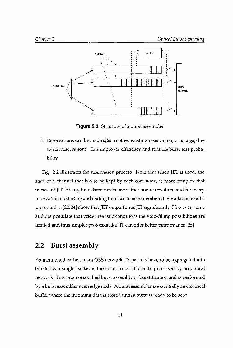
Figure 2 3 Structure of a burst assembler
3 Reservations can be made after another existing reservation, or in a gap be
tween reservations This improves efficiency and reduces burst loss proba
bility
Fig 2 2 illustrates the reservation process Note that when JET is used, the
state of a channel that has to be kept by each core node, is more complex that
m case of JIT At any time there can be more that one reservation, and for every
reservation its startmg and endmg time has to be remembered Simulation results
presented m [22,24] show that JET outperforms JIT significantly However, some
authors postulate that under realistic conditions the void-filling possibilities are
limited and thus simpler protocols like JIT can offer better performance [25]
2.2 Burst assembly
As mentioned earlier, m an OBS network, IP packets have to be aggregated into
bursts, as a smgle packet is too small to be efficiently processed by an optical
network This process is called burst assembly or burstification and is performed
by a burst assembler at an edge node A burst assembler is essentially an electrical
buffer where the incoming data is stored until a burst is ready to be sent
11
Chapter 2 Optical Burst Switching
Data packets grouped within a burst need to have at least one common char
acteristic - destination This means that m each node, there has to be at least one
assembler for each other edge node There may be more assemblers than that if,
for example, packets belongmg to different classes have to be separated from each
other or if it is desirable to group packets accordmg to any other characteristic
It has been postulated [26] that the assembly process can reduce the self-
similarity of aggregated IP traffic However, subsequent research [27,28] suggests
that it is not the case
A structure of a generic burst assembler is shown m Fig 2 3 Incoming IP
packets are first directed to an appropriate queue accordmg to their characteris
tics At a certain time all packets from a given queue are transmitted together as
a burst, the queue is emptied and the assembly process is repeated
Burst assembly has to balance the need for large bursts (to lower overhead)
and low delay There may also be other considerations, for example it can be
used as a part of a Quality of Service scheme The rest of this section will show
how different assembly algorithms achieve those goals
2.2.1 Time and size - based algorithms
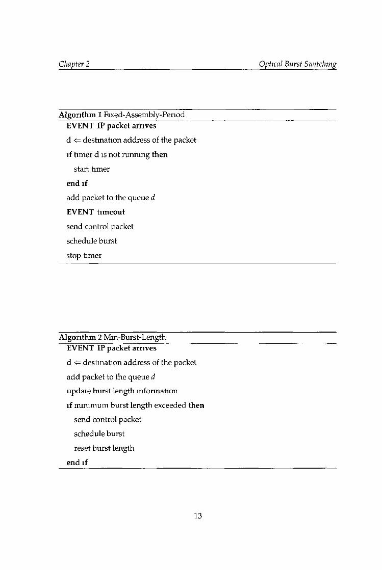
The Fixed-Assembly-Period (FAP) [29] algorithm, as its name implies, stores the
incoming packets for a certain, pre-determined time At the timeout, the burst
is sent, regardless of its size This means that bursts are generated at regular
intervals, and may result m sending very large bursts if at a given time the load
is high Round-robm burst assembly, proposed by Tachibana et al is a variant of
the FAP algorithm [30] Similar algorithm has also been proposed m [31]
Mm-BurstLength [29] is an alternative algorithm, based on size threshold
IP packets are buffered until the size of the burst exceeds some pre-determmed
value In this case, the burst size is almost constant, and interarrival time variable
One possible disadvantage of this approach is that, for low loads, the assembly
delay may be excessively high A similar algorithm has been proposed m [32]
12
Chapter 2 Optical Burst Switching
Algorithm 1 Fixed-Assembly-Period EVENT IP packet arrives
d <= destination address of the packet
if timer d is not running then
start timer
end if
add packet to the queue d
EVENT timeout
send control packet
schedule burst
stop timer
Algorithm 2 Mm-Burst- Length EVENT IP packet arrives
d <= destination address of the packet
add packet to the queue d
update burst length information
if minimum burst length exceeded then
send control packet
schedule burst
reset burst length
end if
13
Chapter 2 Optical Burst Switching
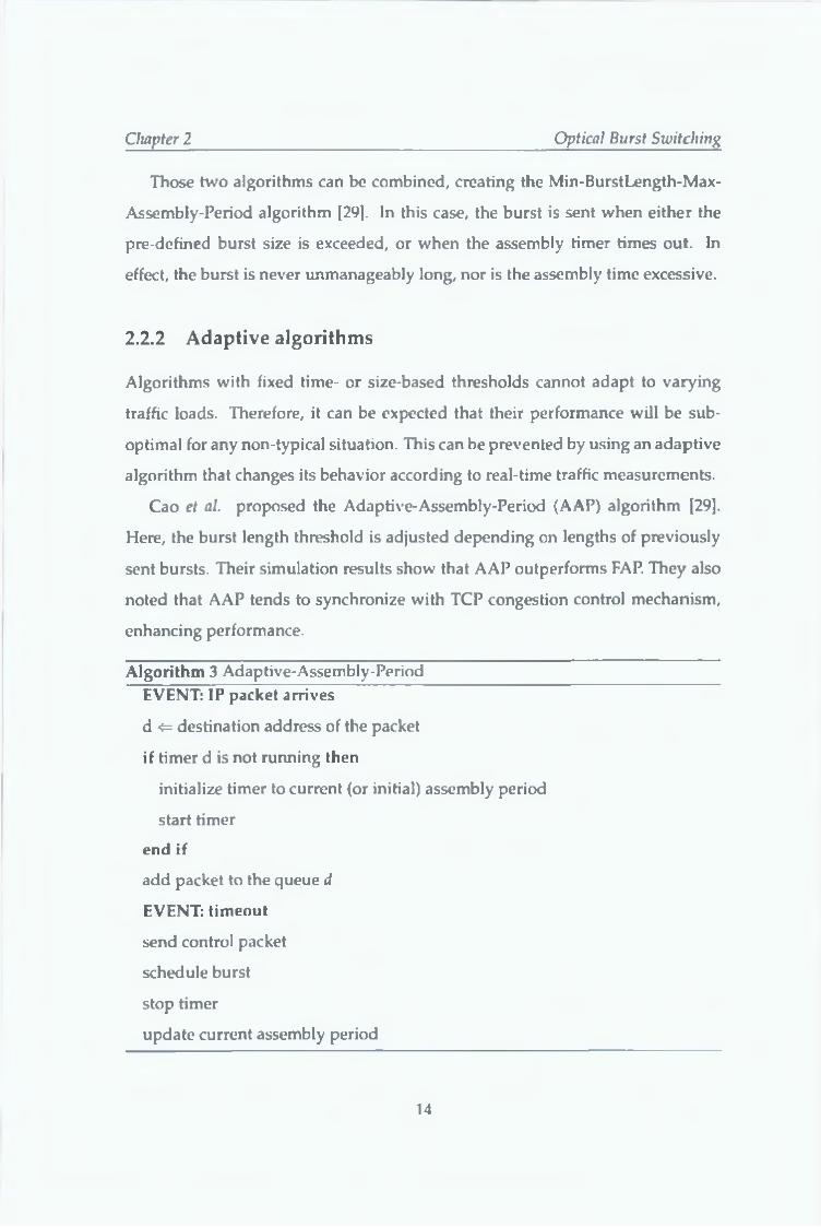
Those two algorithms can be combined, creating the Min-BurstLength-Max-
Assembly-Period algorithm [29]. In this case, the burst is sent when either the
pre-defined burst size is exceeded, or when the assembly timer times out. In
effect, the burst is never unmanageably long, nor is the assembly time excessive.
2.2.2 Adaptive algorithms
Algorithms with fixed time- or size-based thresholds cannot adapt to varying
traffic loads. Therefore, it can be expected that their performance will be sub-
optimal for any non-typical situation. This can be prevented by using an adaptive
algorithm that changes its behavior according to real-time traffic measurements.
Cao el a l proposed the Adaptive-Assembly-Period (AAP) algorithm [29].
Here, the burst length threshold is adjusted depending on lengths of previously
sent bursts. Their simulation results show that AAP outperforms FAP. They also
noted that AAP tends to synchronize with TCP congestion control mechanism,
enhancing performance.
A lg o rith m 3 Adaptive-Assembly-Period EVENT: IP p ack e t arrives
d <= destination address of the packet
if timer d is not running th e n
initialize timer to current (or initial) assembly period
start timer
e n d if
add packet to the queue d
EVENT: tim e o u t
send control packet
schedule burst
stop timer
update current assembly period
14
Chapter 2 Optical Burst Switching
Another, hysteresis-based adaptive assembly algorithm has been proposed by
S Oh et al in [33] Here, the maximum burst size is adjusted m steps, depending
on sizes of previous bursts Also, to avoid excessive assembly times in case of low
load, a timer is used
2.2.3 Composite burst assembly
Burst assembly algorithm may constitute a part of Quality of Service scheme VM
Vokkarane et al proposed the idea of composite burst assembly [34], where packets
belonging to different QoS classes are placed into the same burst They are ar
ranged in such a way, that the low priority packets are grouped in the tail of the
burst Alternatively, if there are more than two classes, the packets are arranged
m order of decreasing priority Later, the policies used withm the network make
the tail more likely to be dropped Details of this and other QoS schemes will be
discussed in Chapter 3
2 2 4 Predictive burst assembly
There are three mam sources of delay in Optical Burst-Switched networks queu
ing delay, offset time and propagation delay Of these, the propagation delay
cannot be changed, but it is possible to manipulate the other two
Typically the sequence of events is as follows IP packets start arriving at
the edge node where they are stored until burst assembly is completed Then,
a control packet is sent with a reservation request Processing the packet and
setting up the route takes a certain time, and while this is bemg done the burst
waits in a buffer at the edge node Finally, after some pre-determmed offset time,
the burst is sent
It is possible to improve this mechamsm if we take into account the fact that
IP traffic can be fairly accurately predicted, at least m a short timescale Then
the size of burst and the time of its assembly bemg finished can be guessed with
15
Chapter 2 Optical Burst Switching
IP pack«»
control packet sent after the butsl assembly ts complete
no prediction
data burst
prediction
control packci vent before the bun* assembly ts complete
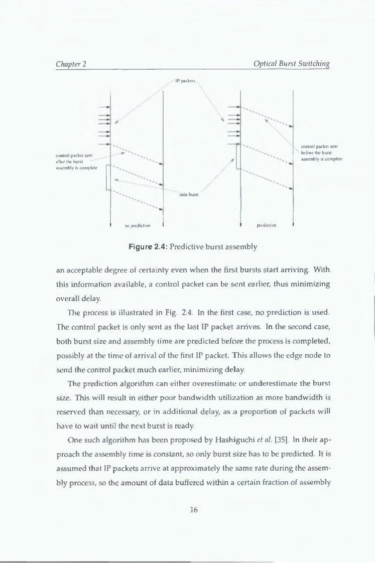
Figure 2.4: Predictive burst assembly
an acceptable degree of certainty even when the first bursts start arriving. With
this information available, a control packet can be s<?nt earlier, thus minimizing
overall delay.
The process is illustrated in Fig. 2.4. In the first case, no prediction is used.
The control packet is only sent as the last IP packet arrives. In the second case,
both burst size and assembly time are predicted before the process is completed,
possibly at the time of arrival of the first IP packet. This allows the edge node to
send the control packet much earlier, minimizing delay.
The prediction algorithm can either overestimate or underestimate the burst
size. This will result in either poor bandwidth utilization as more bandwidth is
reserved than necessary, or in additional delay, as a proportion of packets will
have to wait until the next burst is ready.
One such algorithm has been proposed by Hashiguchi et al. [351. In their ap
proach the assembly time is constant, so only burst size has to be predicted. It is
assumed that IP packets arrive at approximately the same rate during the assem
bly process, so the amount of data buffered within a certain fraction of assembly
16
Chapter 2 Optical Burst Switching
time can be used to estimate the total burst length
It has been proposed that a linear predictor can be used to predict network
traffic [36-38] Morato et al used this technique in burst assembly [39] and found
that it reduces end-to-end delay while maintaining low bandwidth waste
2.3 Node architecture
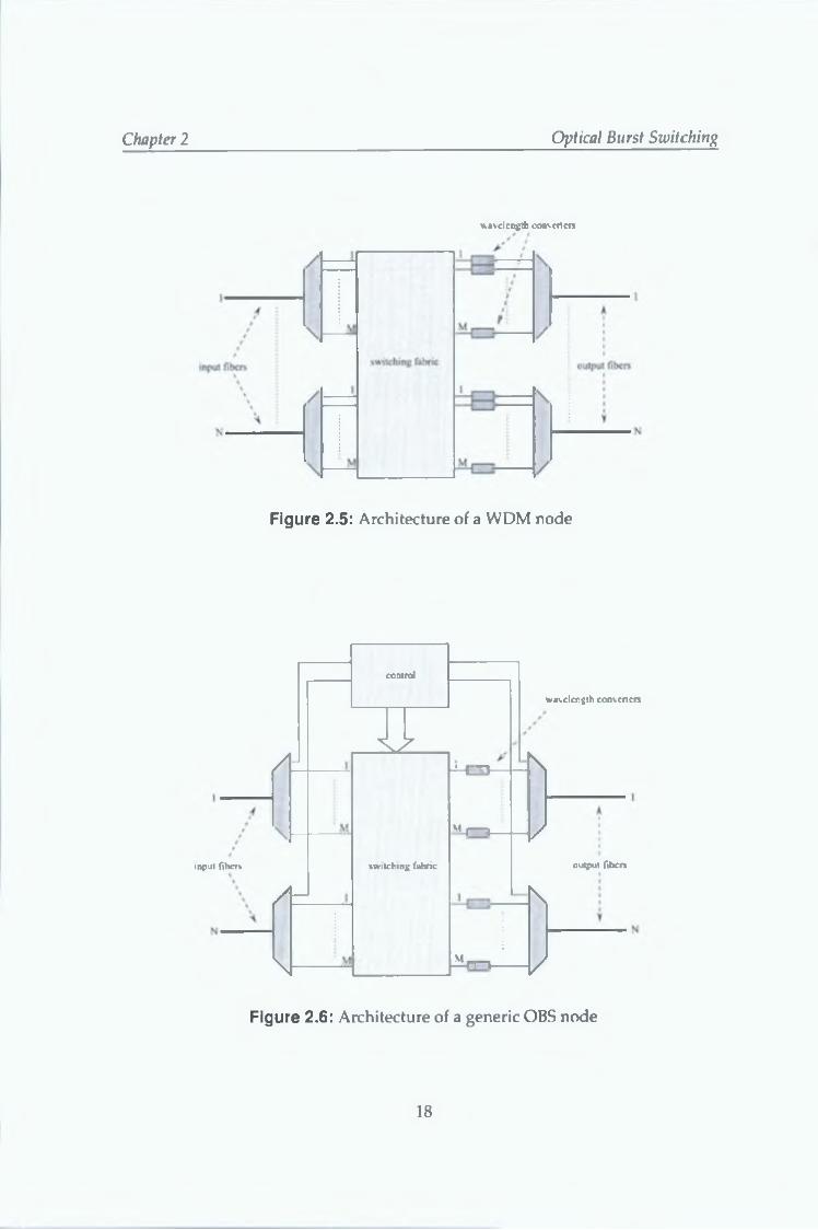
A WDM node should be capable of switching any wavelength from any input
port to any wavelength in any output port A typical example of such a node
is presented m Fig 2 5 The incoming signal is first split into individual wave
lengths and then fed into the switching matrix Then, after being routed to the
appropriate output port, each wavelength is - if necessary - converted to another
channel and sent to an output fiber
OBS network characteristics place additional requirements on a node that is
to be used in such a network First of all, information incoming in a control chan
nel needs to be extracted and analyzed, and then sent again to an appropriate
downstream node A node capable of performmg this function is presented in
Fig 2 6
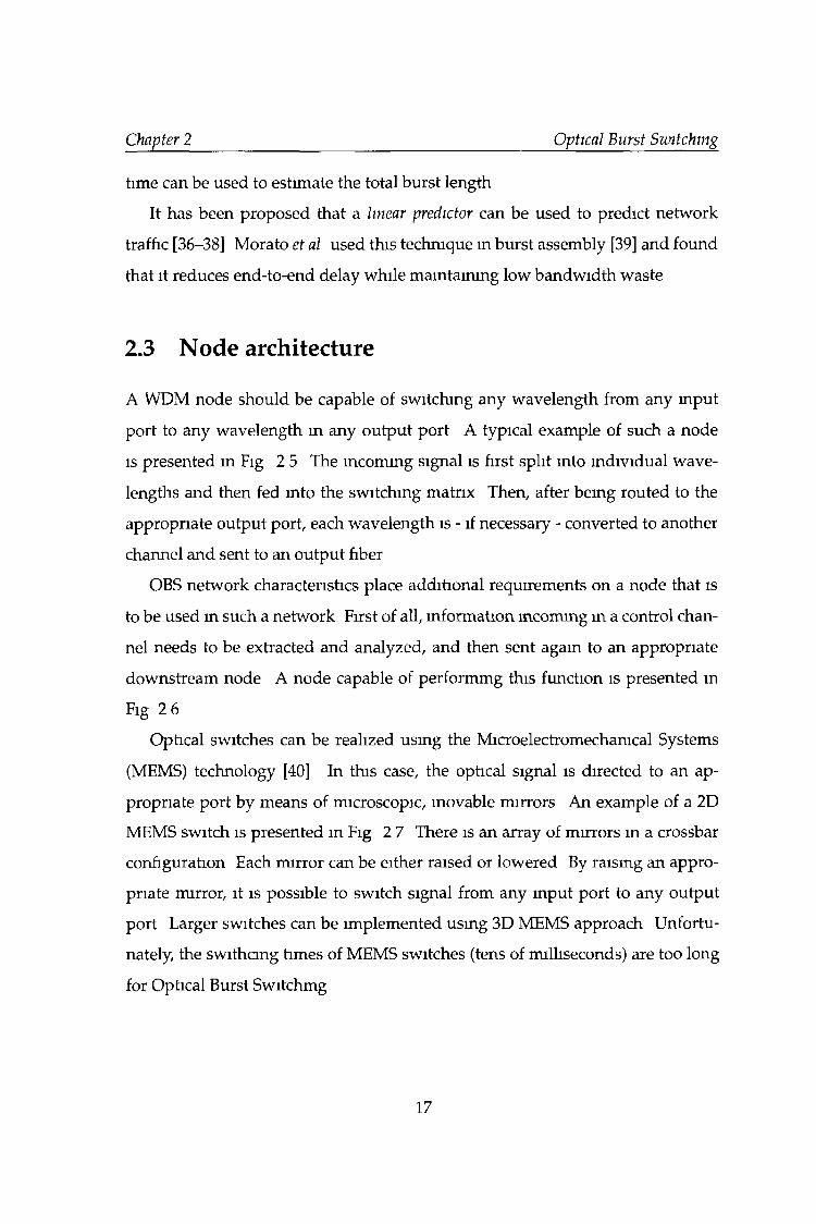
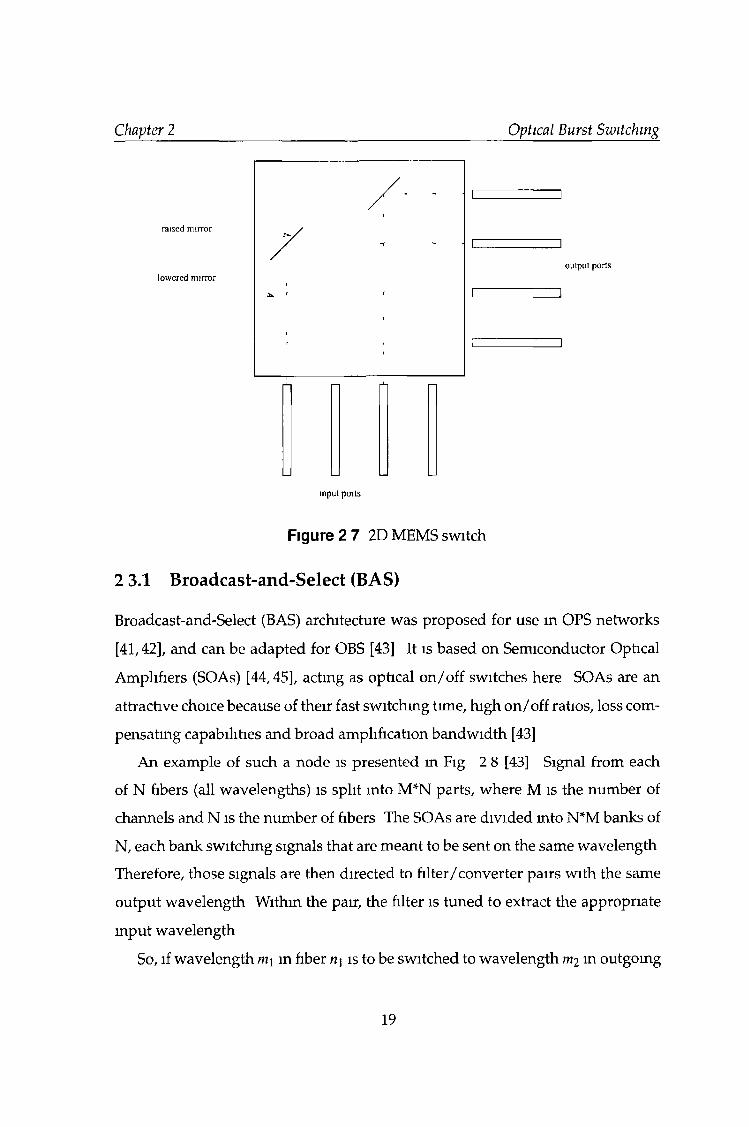
Optical switches can be realized using the Microelectromecharucal Systems
(MEMS) technology [40] In this case, the optical signal is directed to an ap
propriate port by means of microscopic, movable mirrors An example of a 2D
MEMS switch is presented in Fig 2 7 There is an array of mirrors in a crossbar
configuration Each mirror can be either raised or lowered By raising an appro
priate mirror, it is possible to switch signal from any input port to any output
port Larger switches can be implemented using 3D MEMS approach Unfortu
nately, the swithcmg times of MEMS switches (tens of milliseconds) are too long
for Optical Burst Switchmg
17
Chapter 2 Optica! Burst Switching
wavelength conveners
Figure 2.5: Architecture of a WDM node
/
inpul fibers
/
\
control
H
switching fabric
-M _=>
s,-i— \-
wavclcngth conveners
\
M. ,— r v-
/
\
output fibers
/
Figure 2.6: Architecture of a generic OBS node
18
Chapter 2 Optical Burst Switching
raised mirror
lowered mirror
input ports
Figure 2 7 2D MEMS switch
2 3.1 Broadcast-and-Select (BAS)
Broadcast-and-Select (BAS) architecture was proposed for use in OPS networks
[41,42], and can be adapted for OBS [43] It is based on Semiconductor Optical
Amplifiers (SOAs) [44,45], acting as optical on/off switches here SO As are an
attractive choice because of their fast switching time, high on/off ratios, loss com
pensating capabilities and broad amplification bandwidth [43]
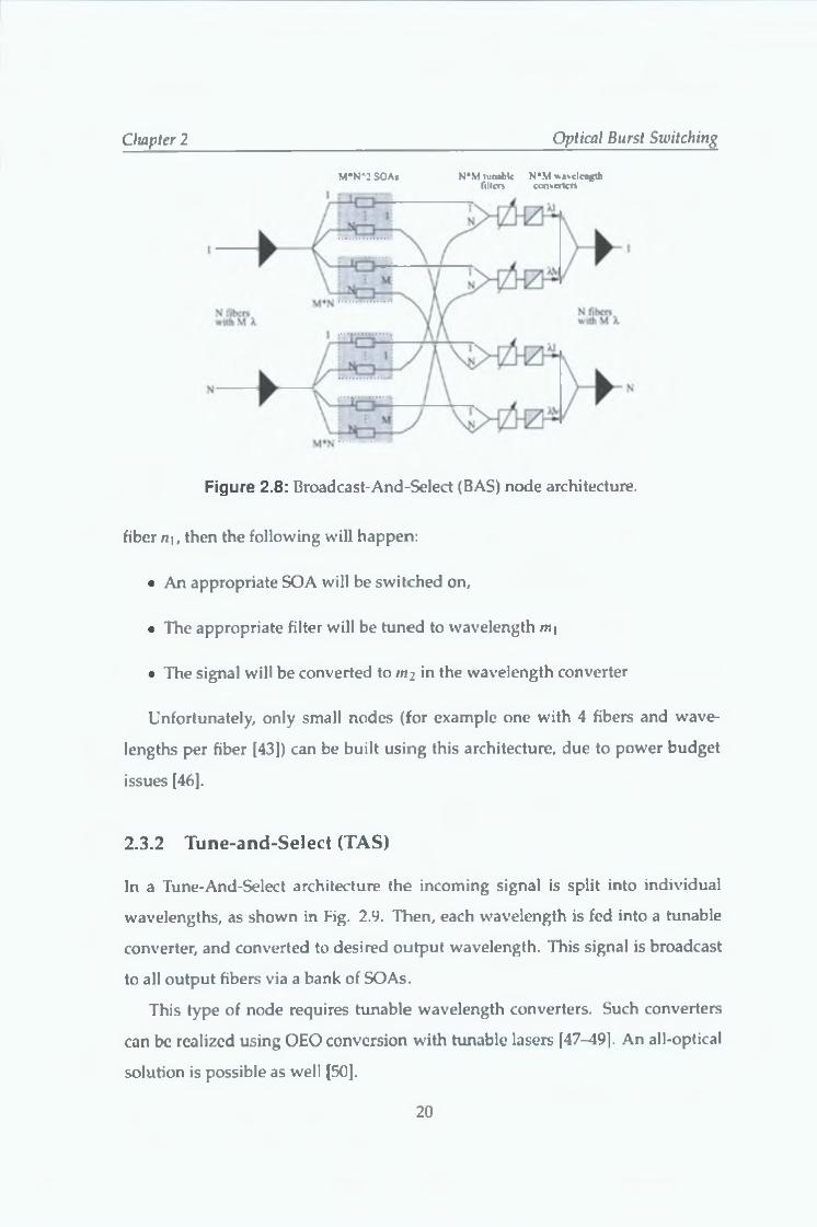
An example of such a node is presented m Fig 2 8 [43] Signal from each
of N fibers (all wavelengths) is split into M*N parts, where M is the number of
channels and N is the number of fibers The SOAs are divided mto N*M banks of
N, each bank switching signals that are meant to be sent on the same wavelength
Therefore, those signals are then directed to filter/converter pairs with the same
output wavelength Within the pair, the filter is tuned to extract the appropriate
m put wavelength
So, if wavelength m\ in fiber n\ is to be switched to wavelength m2 in outgoing
19
Chapiter 2 Optical Burst Switching
M*N*2 SOA* N*M tunable N*M wavelengthfilters converters
Figure 2.8: Broadcast-And-Select (BAS) node architecture,
fiber n\, then the following will happen:
• An appropriate SOA will be switched on,
• The appropriate filter will be tuned to wavelength mi
• The signal will be converted to m2 in the wavelength converter
Unfortunately, only small nodes (for example one with 4 fibers and wave
lengths per fiber [43]) can be built using this architecture, due to power budget
issues [46].
2.3.2 Tune-and-Select (TAS)
In a Tune-And-Select architecture the incoming signal is split into individual
wavelengths, as shown in Fig. 2.9. Then, each wavelength is fed into a tunable
converter, and converted to desired output wavelength. This signal is broadcast
to all output fibers via a bank of SO As.
This type of node requires tunable wavelength converters. Such converters
can be realized using OEO conversion with tunable lasers [47-49]. An all-optical
solution is possible as well [50].
2 0
Chapter 2 Optical Burst Switching
M*N tunable M*NA2 SOAswavclcn^ht converters
Figure 2 9 Tune-And-Select (TAS) node architecture
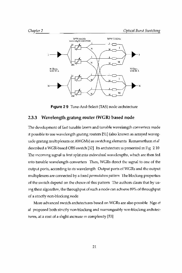
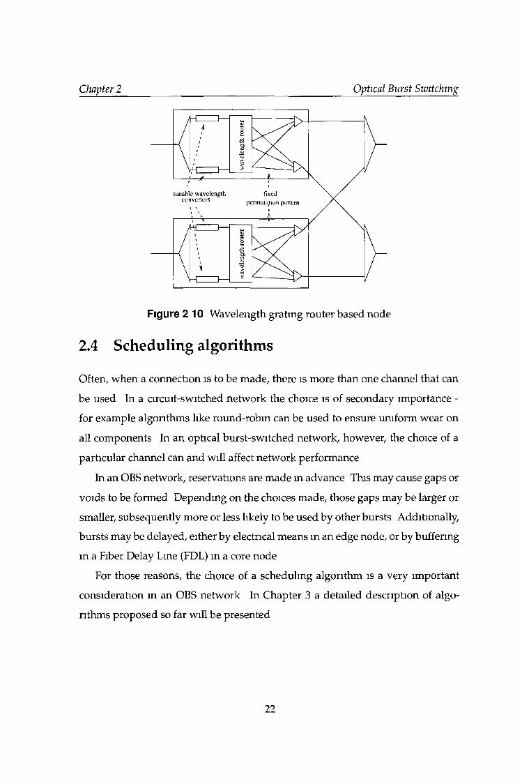
2.3.3 Wavelength grating router (WGR) based node
The development of fast tunable lasers and tunable wavelength converters made
it possible to use wavelength grating routers [51] (also known as arrayed waveg
uide grating multiplexers or AWGMs) as switching elements Ramamirtham et al
described a WGR-based OBS switch [52] Its architecture is presented m Fig 2 10
The incoming signal is first split into individual wavelengths, which are then fed
into tunable wavelength converters Then, WGRs direct the signal to one of the
output ports, according to its wavelength Output ports of WGRs and the output
multiplexers are connected by a fixed permutation pattern The blocking properties
of the switch depend on the choice of this pattern The authors claim that by us
ing their algorithm, the throughput of such a node can achieve 89% of throughput
of a strictly non-blockmg node
More advanced switch architectures based on WGRs are also possible Ngo et
al proposed both strictly non-blocking and rearrangeably non-blockmg architec
tures, at a cost of a slight increase in complexity [53]
21
Chapter 2 Optical Burst Switching
Figure 2 10 Wavelength grating router based node
2.4 Scheduling algorithms
Often, when a connection is to be made, there is more than one channel that can
be used In a circuit-switched network the choice is of secondary importance -
for example algorithms like round-robin can be used to ensure uniform wear on
all components In an optical burst-switched network, however, the choice of a
particular channel can and will affect network performance
In an OBS network, reservations are made in advance This may cause gaps or
voids to be formed Depending on the choices made, those gaps may be larger or
smaller, subsequently more or less likely to be used by other bursts Additionally,
bursts may be delayed, either by electrical means m an edge node, or by buffering
in a Fiber Delay Lme (FDL) in a core node
For those reasons, the choice of a scheduling algorithm is a very important
consideration in an OBS network In Chapter 3 a detailed description of algo
rithms proposed so far will be presented
22
Chapter 2 Optical Burst Switching
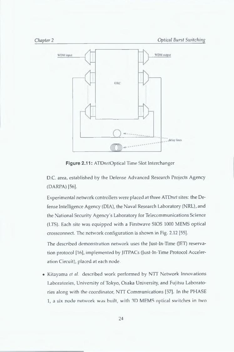
2.5 Time Sliced Optical Burst Switching (TSOBS)
In an OBS node, a burst arriving on wavelength n might need to be converted
to wavelength m in case of a contention. This operation is done by a wavelength
converter. Unfortunately, those devices are considered to be the largest single cost
component of an optical node. Therefore it was proposed by Ramamirtham et
al. to replace wavelength conversion with switching in time domain [54]. In
their approach, each wavelength carries a structure of time slots of equal length.
A sequence of slots in consecutive frames is called a channel. A control packet
carries information about the incoming burst:
• its arrival time,
• its channel (i.e. slot number),
• its length (i.e. number of slots).
A key building block of TSOBS router is an Optical Time Slot Interchanger (OTSI).
It is capable of delaying the contents of time slots by different amounts of time,
thus changing their relative positions. The structure of an OTSI is shown in Fig
2.11.
The authors claim that their solution offers good statistical multiplexing per
formance without the need for costly wavelength converters.
2.6 OBS testbeds
Presently, there are no functioning large-scale OBS networks. However, several
laboratory testbeds have been implemented:
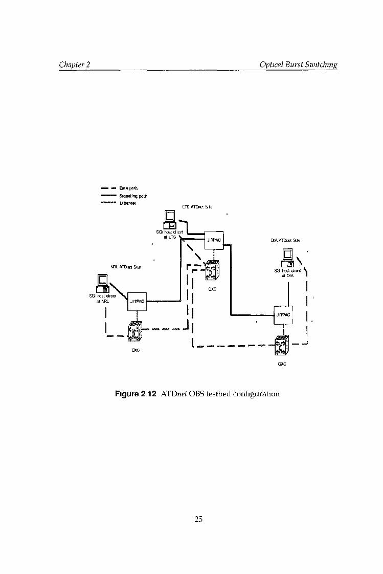
• Baldine et al. described an OBS demonstration network overlaying the Ad
vanced Technology Demonstration Network (ATDnef) all-optical testbed
[55]. ATDwcf is high performance networking testbed in the Washington
23
Chapter 2 Optical Burst Switching
Figure 2.11: ATDncf Optical Time Slot Interchanger
D.C. area, established by the Defense Advanced Research Projects Agency
(DARPA) (56).
Experimental network controllers were placed at three AJDnet sites: the De
fense Intelligence Agency (DIA), the Naval Research Laboratory (NRL), and
the National Security Agency's Laboratory for Telecommunications Science
(LTS). Each site was equipped with a Firstwave SIOS 1000 MEMS optical
crossconnect. The network configuration is shown in Fig. 2.12 [55].
The described demonstration network uses the Just-In-Time OFT) reserva
tion protocol [16], implemented by JITPACs (Just-In-Time Protocol Acceler
ation Circuit), placed at each node.
• Kitayama et al. described work performed by NTT Network Innovations
Laboratories, University of Tokyo, Osaka University, and Fujitsu Laborato
ries along with the coordinator, NTT Communications [57]. In the PHASE
1, a six node network was built, with 3D MFMS optical switches in two
24
Chapter 2 Optical Burst Switching
—»* — Data path
— Signaling path Ethernet
ITS ATDnet Site
oxc
Figure 2 12 ATDnet OBS testbed configuration
25
Chapter 2 Optical Burst Switching
nodes, and planar lightwave circuit (PLC) switches in four nodes The over
all switching tune was 30 ms and the network throughput of 0 87 was ob
tained
• Sim et al built an OBS testbed, consisting of one core node and three edge
nodes [58] The architectures of both types of nodes were discussed, along
with the format of data burst and control packet The switching time of 3ms
was achieved using thermo-optic switches
2.7 Summary
In this chapter the fundamentals of Optical Burst-Switched networks were intro
duced In particular the evolution of optical networks and motivation for optical
burst switching were discussed The basic OBS protocol (JIT and JET) were de
scribed along wit their respective advantages and disadvantages The following
sections dealt with burst assembly algorithms and OBS node architecture Fi
nally, an OBS variant called Time Sliced Optical Burst Switching was introduced
and several existing OBS testbeds were described
26
Chapter 3
Scheduling algorithms and Quality
of Service
The first part of this chapter explains the importance of scheduling m Optical
Burst-Switched networks and describes m detail several scheduling algorithms
Distinction is made between legacy scheduling algorithms and dedicated OBS al
gorithms The latter are further divided into per-burst algorithms and batch or
group scheduling algorithms Additionally, a rescheduling algorithm is described
The second part of this chapter deals with Quality of Service provisioning
m Optical Burst-Switched networks Starting with the popular offset-based QoS
scheme, several other approaches are described, including composite burst assem
bly and intentional burst dropping
3.1 Scheduling algorithms
The scheduling decision is of a particular importance in Optical Burst Switching
networks This is because reservations are made m advance The control packet,
carrying information about the data burst arrives ahead of it Therefore, when a
reservation request arrives with a relatively small offset time, it is possible that
there are other existing reservations m the future In other words, there may be
available voids or gaps Creation of large gaps is considered undesirable, as their
bandwidth is likely to be wasted
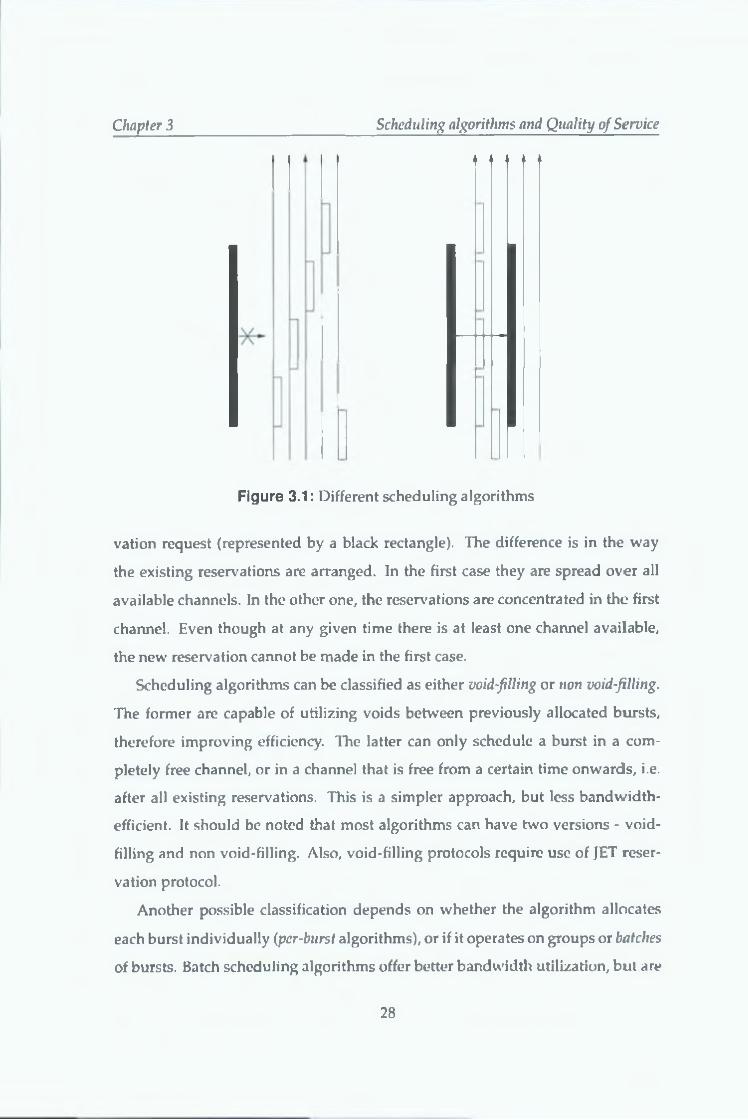
Fig 3 1 shows two examples of burst scheduling In both cases there are five
existing reservations (represented by unfilled rectangles) and one incoming reser-
27
C h a p te r 3 Scheduling algorithms and Quality of Service
Figure 3.1: Different scheduling algorithms
vation request (represented by a black rectangle). The difference is in the way
the existing reservations are arranged. In the first case they are spread over all
available channels. In the other one, the reservations are concentrated in the first
channel. Even though at any given time there is at least one channel available,
the new reservation cannot be made in the first case.
Scheduling algorithms can be classified as either void-filling or non void-filling.
The former are capable of utilizing voids between previously allocated bursts,
therefore improving efficiency. The latter can only schedule a burst in a com
pletely free channel, or in a channel that is free from a certain time onwards, i.e.
after all existing reservations. This is a simpler approach, but less bandwidth-
efficient. It should be noted that most algorithms can have two versions - void-
filling and non void-filling. Also, void-filling protocols require use of JET reser
vation protocol.
Another possible classification depends on whether the algorithm allocates
each burst individually (per-burst algorithms), or if it operates on groups or batches
of bursts. Batch scheduling algorithms offer better bandwidth utilization, but are
28
Chapter 3 Scheduling algorithms and Quality of Service
usually more complex and introduce additional delay
3 1.1 Legacy scheduling algorithms
Certain well-known algorithms, for example those used m traditional telephony
can be used m burst-switched networks While not necessarily optimal for optical
burst switching, their behavior is well-studied and they are generally uncompli
cated
• First Fit - the channels are checked in some pre-determined order, most
likely from the lowest numbered one to the highest one The new burst
is allocated in the first available channel
• Most Used - the average load m each channel is measured m a certain time
wmdow The connection attempts are made m order of decreasing channel
load
• Random - connection attempts are made m a random order
• Round Robm - the channels are checked in a pre-determined order, but the
starting pomt changes with each attempt
Of the algorithms listed above, First Fit and Most Used tend to concentrate
traffic m a certain set of channels This results m a better performance than in
the case of Random and Round Robm, which use all wavelength channels evenly
[59]
3 1 2 Per-burst scheduling algorithms
Per-burst scheduling algorithms schedule one burst at a time, takmg mto account
only existing reservations The decision is made as soon as possible and a control
packet is sent to the downstream node immediately afterwards This approach
mtroduces mmimal delay, but is less bandwidth-efficient than batch scheduling,
discussed later m this chapter
29
Chapter 3 Scheduling algorithms and Quality of Service
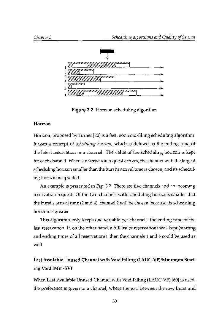
Figure 3 2 Horizon scheduling algorithm
Horizon
Horizon, proposed by Turner [20] is a fast, non void-filling schedulmg algorithm
It uses a concept of scheduling horizon, which is defmed as the ending time of
the latest reservation m a channel The value of the schedulmg horizon is kept
for each channel When a reservation request arrives, the channel with the largest
schedulmg horizon smaller than the burst's arrival time is chosen, and its schedul
mg horizon is updated
An example is presented m Fig 3 2 There are five channels and an incoming
reservation request Of the two channels with schedulmg horizons smaller that
the burst's arrival time (2 and 4), channel 2 will be chosen, because its schedulmg
horizon is greater
This algorithm only keeps one variable per channel - the ending time of the
last reservation If, on the other hand, a full list of reservations was kept (startmg
and ending times of all reservations), then the channels 1 and 5 could be used as
well
Last Available Unused Channel with Void Filling (LAUC-VF)/Minimum Start
mg Void (Mm-SV)
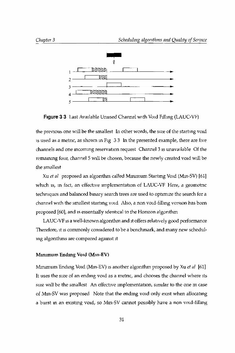
When Last Available Unused Channel with Void Filling (LAUC-VF) [60] is used,
the preference is given to a channel, where the gap between the new burst and
30
Chapter 3 Scheduling algorithms and Quality of Service
Figure 3 3 Last Available Unused Channel with Void Filling (LAUC-VF)
the previous one will be the smallest In other words, the size of the starting void
is used as a metric, as shown m Fig 3 3 In the presented example, there are five
channels and one incoming reservation request Channel 3 is unavailable Of the
remaining four, channel 5 will be chosen, because the newly created void will be
the smallest
Xu et al proposed an algorithm called Minimum Starting Void (Min-SV) [61]
which is, in fact, an effective implementation of LAUC-VF Here, a geometric
techniques and balanced binary search trees are used to optimize the search for a
channel with the smallest startmg void Also, a non void-filling version has been
proposed [60], and is essentially identical to the Horizon algorithm
LAUC-VF is a well-known algorithm and it offers relatively good performance
Therefore, it is commonly considered to be a benchmark, and many new schedul
ing algorithms are compared agamst it
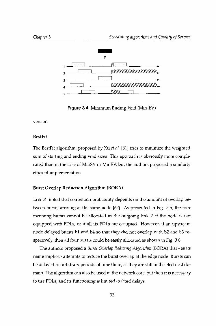
Minimum Ending Void (Mm-EV)
Minimum Ending Void (Mm-EV) is another algorithm proposed by Xu et al [61]
It uses the size of an endmg void as a metric, and chooses the channel where its
size will be the smallest An effective implementation, similar to the one m case
of Mm-SV was proposed Note that the endmg void only exist when allocating
a burst in an existmg void, so Mm-SV cannot possibly have a non void-fillmg
31
Chapter 3 Scheduling algorithms and Quality of Service
Figure 3 4 Minimum Ending Void (Min-EV)
version
BestFit
The BestFit algorithm, proposed by Xu et al [61] tries to minimize the weighted
sum of starting and endmg void sizes This approach is obviously more compli
cated than m the case of MinSV or MmEV, but the authors proposed a similarly
efficient implementation
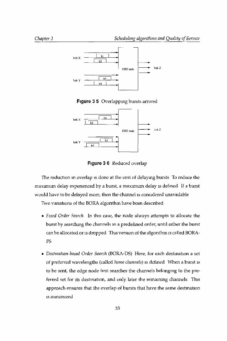
Burst Overlap Reduction Algorithm (BORA)
Li et al noted that contention probability depends on the amount of overlap be
tween bursts arrivmg at the same node [62] As presented m Fig 3 5, the four
mcommg bursts cannot be allocated m the outgoing link Z if the node is not
equipped with FDLs, or if all its FDLs are occupied However, if an upstream
node delayed bursts b l and b4 so that they did not overlap with b2 and b3 re
spectively, then all four bursts could be easily allocated as shown in Fig 3 6
The authors proposed a Burst Overlap Reducing Algol ithm (BORA) that - as its
name implies - attempts to reduce the burst overlap at the edge node Bursts can
be delayed for arbitrary periods of time there, as they are still m the electrical do
main The algorithm can also be used m the network core, but then it is necessary
to use FDLs, and its functioning is limited to fixed delays
32
Chapter 3 Scheduling algorithms and Quality of Service
Figure 3 5 Overlapping bursts arrived
Figure 3 6 Reduced overlap
The reduction in overlap is done at the cost of delaying bursts To reduce the
maximum delay experienced by a burst, a maximum delay is defined If a burst
would have to be delayed more, then the channel is considered unavailable
Two variations of the BORA algorithm have been described
• Fixed Order Search In this case, the node always attempts to allocate the
burst by searchmg the channels m a predefined order, until either the burst
can be allocated or is dropped This version of the algorithm is called BORA-
FS
• Destination-based Order Search (BORA-DS) Here, for each destination a set
of preferred wavelengths (called home channels) is defmed When a burst is
to be sent, the edge node first searches the channels belonging to the pre
ferred set for its destination, and only later the remaining channels This
approach ensures that the overlap of bursts that have the same destination
is m inim ized
33
Chapter 3 Scheduling algorithms and Quality of Service
Additionally, both versions can be either void filling or non-void filling The
authors provided simulation results proving that both BORA-FS-VF and BORA-
DS-VF overperform LAUC-VF m terms of burst loss probability The difference
is particularly big (two orders of magmtude) for small loads
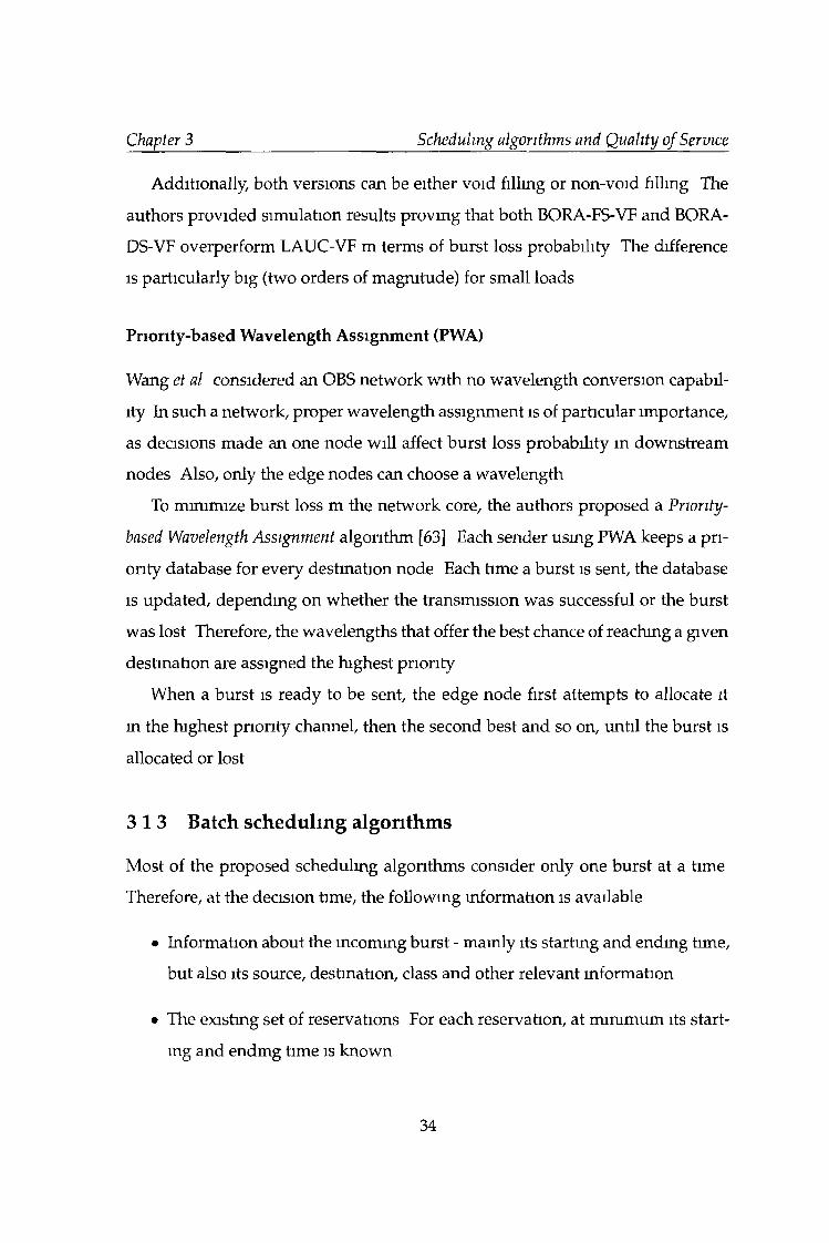
Priority-based Wavelength Assignment (PWA)
Wang et al considered an OBS network with no wavelength conversion capabil
ity In such a network, proper wavelength assignment is of particular importance,
as decisions made an one node will affect burst loss probability in downstream
nodes Also, only the edge nodes can choose a wavelength
To minimize burst loss m the network core, the authors proposed a Priority-
based Wavelength Assignment algorithm [63] Each sender using PWA keeps a pri
ority database for every destination node Each time a burst is sent, the database
is updated, depending on whether the transmission was successful or the burst
was lost Therefore, the wavelengths that offer the best chance of reaching a given
destination are assigned the highest priority
When a burst is ready to be sent, the edge node first attempts to allocate it
m the highest priority channel, then the second best and so on, until the burst is
allocated or lost
3 1 3 Batch scheduling algorithms
Most of the proposed scheduling algorithms consider only one burst at a time
Therefore, at the decision time, the following information is available
• Information about the incoming burst - mainly its starting and endmg time,
but also its source, destination, class and other relevant information
• The existmg set of reservations For each reservation, at minimum its start
ing and endmg time is known
34
Chapter 3 Scheduling algorithms and Quality o f Service
________________________________________________________________I 1 f lm ll I______
________________________________________ I I_____________________________
____________________________ I 1 M u t t f t I_________________________________________________________________________ _
__________ I 4 d itv . Q . 1--------------------------------------____________________________I < r l u t 1 I_________________________________________________________________________
1 f t r i m D 1________________________________________________________________________________________
Figure 3.7: Waiting-Queuing-Scheduling algorithm.
Unfortunately, as the decision is made without any delay, no information is
available about future reservation requests. This results in a suboptimal alloca
tion of bursts. An alternative approach is called batch scheduling. Here, after a
control packet is received, it is delayed before the decision is made. During this
delay, other control packets are received and likewise delayed. In effect, when the
burst is about to be scheduled, the following information can be utilized:
• Information about the burst itself.
• The existing set of reservations.
• Information about bursts that will be scheduled during a period of time
equal to the scheduling delay
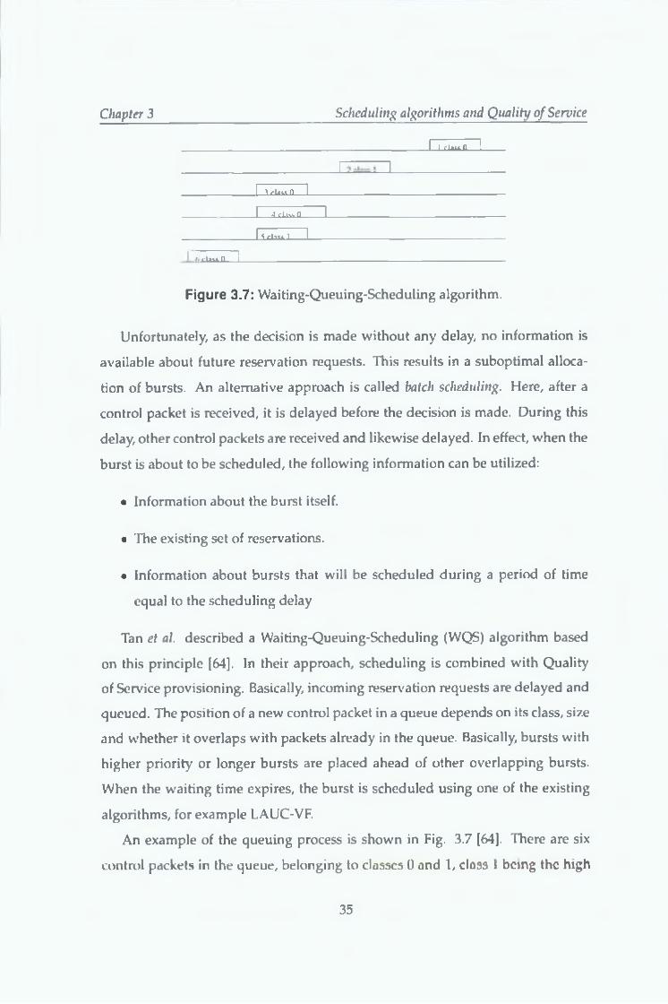
Tan et al. described a Waiting-Queuing-Scheduling (WQS) algorithm based
on this principle [64]. In their approach, scheduling is combined with Quality
of Service provisioning. Basically, incoming reservation requests are delayed and
queued. The position of a new control packet in a queue depends on its class, size
and whether it overlaps with packets already in the queue. Basically, bursts with
higher priority or longer bursts are placed ahead of other overlapping bursts.
When the waiting time expires, the burst is scheduled using one of the existing
algorithms, for example LAUC-VF.
An example of the queuing process is shown in Fig. 3.7 [64]. There are six
control packets in the queue, belonging to classes 0 and 1, class 1 being the high
35
Chapter 3 Scheduling algorithms and Quality of Service
priority class Control packets 3,4 and 5 overlap Packet 5 belongs to class 1, so it
will be scheduled first, and packet 4 will be the next one, because of its size
It has been demonstrated that this approach can offer low loss ratio m high
priority class and also decrease the total burst loss ratio It supports unlimited
number of traffic classes Its drawbacks include the necessity of using larger offset
times due to the additional delay experienced by control packets
Charcranoon et al proposed a Maximum Stable-Set Interval Scheduling Algo
rithm (MSSIS) [65] Here, mcommg reservation requests are briefly delayed, and
then graph theory is used to schedule them Presented simulation results show
that this approach offers about 5% improvement over traditional immediate reser
vation Another batch scheduling algorithm has been described in [66]
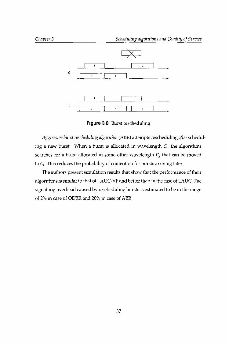
3.1 4 Burst rescheduling algorithms
Once a burst has been scheduled, the possibilities of modifying the reservation
are very limited In particular, changing its arrival time would require usmg
FDLs On the other hand, movmg an existing reservation to another wavelength
(reschedulmg) is easier, and only notifying downstream nodes of the change will
be necessary This may make it possible to schedule a burst that would other
wise be dropped Consider the situation presented m Fig 3 8 a) There are two
channels, four existing reservations and one mcommg reservation request Unfor
tunately, it is not possible to make the reservation But if reservation 3 is resched
uled m the other channel, as presented m Fig 3 8 b), the first channel becomes
available for the new burst
Tan et al proposed two algorithms usmg the idea of rescheduling existing
reservations in order to accommodate new bursts [67] On-demand burst reschedul-
ing algorithm (ODBR) first attempts to schedule the new burst without modifying
existmg reservations Only when it fails, it tries reschedulmg m order to accom
modate the new burst All the wavelengths are tested one by one, and the one
where the newly created void would be the smallest is chosen
36
Chapter 3 Scheduling algorithms and Quality of Service
Figure 3 8 Burst rescheduling
Aggressive burst rescheduling algorithm (ABR) attempts reschedulmg after schedul
ing a new burst When a burst is allocated m wavelength Clf the algorithms
searches for a burst allocated in some other wavelength Cj that can be moved
to Ci This reduces the probability of contention for bursts arriving later
The authors present simulation results that show that the performance of their
algorithms is similar to that of LAUC-VF and better than m the case of LAUC The
signalling overhead caused by reschedulmg bursts is estimated to be in the range
of 2% m case of ODBR and 20% in case of ABR
37
Chapter 3 Scheduling algorithms and Quality of Service
3.2 Quality of service
Quality of Service provisioning is still an important issue m the Internet as many
services, like Voice over IP (VoIP) require certain bandwidth or delay guarantees
On the other hand, bulk data transfers are insensitive to delay and fairly insensi
tive to loss ratio Much effort has been devoted to providmg QoS in the Internet
Unfortunately, most of the proposed schemes are buffer-based In the optical do
main, signal can only be delayed for a short periods in Fiber Delay Lines (FDLs)
This makes those QoS schemes impractical m optical networks
Providmg QoS in OBS networks requires fmdmg new schemes, that either
do not require buffering, or can be used with the limited buffering capability of
FDLs In this chapter several such schemes are described, their areas of applica
tion and potential weaknesses are identified
3 21 Offset-based QoS
In OBS networks, bandwidth is reserved in advance The control packed is fol
lowed by the data packet after a certain period of time, called offset time It has
been noted [9] that loss probability experienced by bursts with larger offset time
is lower than in case of bursts with smaller offset time The logical explanation
of this effect is that if the offset time is relatively large, then bandwidth will be
reserved before other bursts have a chance to make a reservation
Consequently, one of the most widely proposed solutions was to use addi
tional offset time to provide QoS guarantees to certam classes of bursts [68-70]
In this scheme, bursts belonging to high priority classes use larger offset time
than strictly necessary, achievmg a certam degree of isolation from lower-pnority
bursts Yoo et al [70] demonstrated that when burst lengths are exponentially dis
tributed, then usmg additional offset time equal to five times the average burst
length ensures over 99% of class isolation Alternatively, offset time can be ad
justed to achieve desired loss probabilities by usmg a heuristic formula proposed
38
Chapter 3 Scheduling algorithms and Quality o f Service
by So et al. [71]. A detailed analytical model of an offset-based QoS scheme has
been prosented in [72].
A big advantage of this approach is that it exploits effects that are natural
in Optical Burst Switching networks. Therefore, its added functionality resides
at the edge and no modifications in the core of the network are required. The
scheme can support multiple classes of service with good class isolation.
However, there are some disadvantages as well:
• A burst selecting effect has been observed [68]. Offset based QoS scheme
creates significant amount of voids. Due to their presence, loss probability
will be higher in case of longer bursts. This in turn means that the loss
probability alone becomes an unreliable metric of network performance.
• To ensure sufficient class isolation, the additional offset time has to be on
the order of several mean burst lengths [68]. The increase is even bigger if
multiple classes are to be supported. The resulting end-to-end delay in high
priority class may be unacceptable.
• In a complex network, any link may carry aggregated traffic, with bursts
destined to several different edge nodes. As the hop distances to their re
spective destinations are unlikely to be identical, their offset times will vary
as well. This makes it difficult to ensure that traffic classes are isolated in
the entire network.
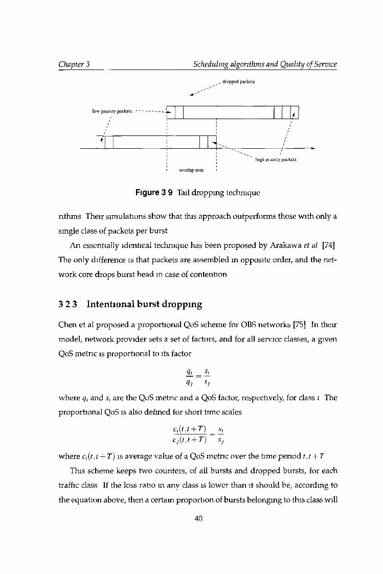
3.2.2 Composite burst assembly
Vokkarane et al. proposed an interesting QoS scheme [34,73], where IP packets
belonging to different classes are assembled into one burst. However, the high
priority packets are placed in the head of the burst, and the low priority pack
ets in its tail. During a contention, only the tail of contending burst is dropped,
as shown in Fig 3.9. Authors proposed several composite burst assembly algo-
39
Chapter 3 Scheduling algorithms and Quality of Service
, dropped packcts
low priority packets
overlap area
high priority packets
Figure 3 9 Tail dropping technique
nthm s Their simulations show that this approach outperforms those with only a
single class of packets per burst
An essentially identical technique has been proposed by Arakawa et al [74]
The only difference is that packets are assembled in opposite order, and the net
work core drops burst head m case of contention
3 2 3 Intentional burst dropping
Chen et al proposed a proportional QoS scheme for OBS networks [75] In their
model, network provider sets a set of factors, and for all service classes, a given
QoS metric is proportional to its factor
Qj ~ s j
where qt and st are the QoS metric and a QoS factor, respectively, for class i The
proportional QoS is also defined for short time scales
ct(t,t + T) = ^C j ( t , t + T) Sj
where , t + T) is average value of a QoS metric over the time period t,t + T
This scheme keeps two counters, of all bursts and dropped bursts, for each
traffic class If the loss ratio in any class is lower than it should be, accordmg to
the equation above, then a certain proportion of bursts belongmg to this class will
40
Chapter 3 Scheduling algorithms and Quality of Service
be intentionally dropped Those counters are periodically reset to make sure that
the most recent history is taken into account
Another QoS scheme utilizing intentional burst dropping was proposed by
Zhang et al [76-78] In this case, the technique is called an early drop scheme and
is used to provide absolute QoS guarantees An early dropping probability is calcu
lated for each class, based on measured loss ratio m the immediate higher class
This mechanism is similar to random early detection (RED), except that conges
tion is detected by measuring loss ratio instead of queue size
Zhou et al suggested that intentional burst dropping can also be used to en
sure fairness m Optical Burst-Switched networks [79]
3 2.4 Assured Horizon
Dolzer proposed a QoS framework called Assured Horizon [31,80] Its functional
ity is split between network edge and network core
• Edge node Incoming packets are classified accordmg to their class and as
sembled separately A fixed-time assembly algorithm is used On timeout,
the assembler checks if the queue size does not exceed its predefined maxi
mum value If not, then the burst is marked as compliant (C) and sent mto
the network Otherwise, the remaining packets will either wait until the
next burst is generated, or, if their total length exceeds a certain threshold,
they will be assembled into separated burst and marked as non-compliant
(NC)
• Core node Each node m the network core is preceded by a burst dropper
When m a regular state, the dropper does not drop any bursts However,
when the number of allocated wavelengths in the node exceeds a certain
threshold, the dropper switches to a congestion state and drops all bursts
marked as NC
41
Chapter 3 Scheduling algorithms and Quality of Service
Simulations prove that this QoS scheme offers service differentiation that can be
adjusted m a wide range, comparable to electrical solutions
3 2 5 Preferred wavelength sets
Wan et al [81] proposed an Optical Burst-Switched network based on dynamic
wavelength routing Their proposal differs from a "standard" OBS network in that
it contains a control node - a central entity that serves as an intermediary in all
reservation requests In other words, the control in the network is centralized
Another difference is that the edge node waits for an acknowledgment before
sendmg data
The authors proposed a Quality of Service scheme based on wavelength quo
tas - dynamic preferred wavelength sets (D-PWS) Basically, for each QoS class, a
floor level and ceiling level of wavelength quota are defmed No traffic class can
be assigned more wavelengths at once than defined by its ceiling level, but at the
same time, the minimum set of wavelengths is guaranteed by the floor level
The authors compare their scheme with a scheme using static preferred wave
length sets (S-PWS) and find that D-PWS can guarantee QoS effectively, and offers
better network utilization than S-PWS
3.2 6 Preemptive wavelength reservation protocol (PWRP)
Liao et al proposed an algorithm called PWRP, capable of providing proportional
QoS for an arbitrary number of traffic classes [82] Each node keeps an usage profile
for each traffic class A class is considered to be in pi ofile if it does not exceed a
predefmed usage limit If a given class is out of profile, then its reservations can
be preempted A simplified diagram of the algorithm is presented m Fig 3 10
If the burst being preempted is already being transmitted, then the node will
send a termination signal, so that downstream nodes learn about the preemp
tion However, if the transmission has not started yet, then no signal will be sent,
42
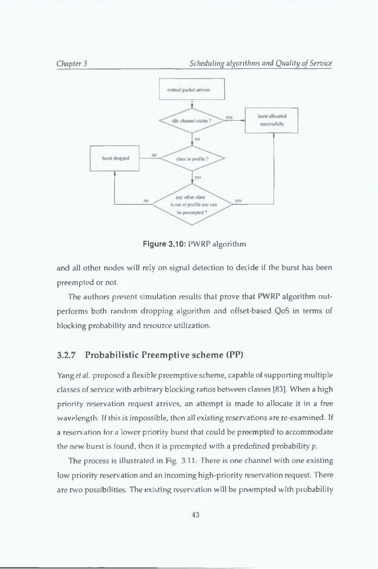
Chapter 3 Scheduling algorithms and Quality of Service
Figure 3.10: PWRP algorithm
and all other nodes will rely on signal detection to decide if the burst has been
preempted or not.
The authors present simulation results that prove that PWRP algorithm out
performs both random dropping algorithm and offset-based QoS in terms of
blocking probability and resource utilization.
3.2.7 Probabilistic Preemptive scheme (PP)
Yang et al. proposed a flexible preemptive scheme, capable of supporting multiple
classes of service with arbitrary blocking ratios between classes [83]. When a high
priority reservation request arrives, an attempt is made to allocate it in a free
wavelength. If this is impossible, then all existing reservations are re-examined. If
a reservation for a lower priority burst that could be preempted to accommodate
the new burst is found, then it is preempted with a predefined probability p.
The process is illustrated in Fig. 3.11. There is one channel with one existing
low priority reservation and an incoming high-priority reservation request. There
are two possibilities. The existing reservation will be preempted with probability
43
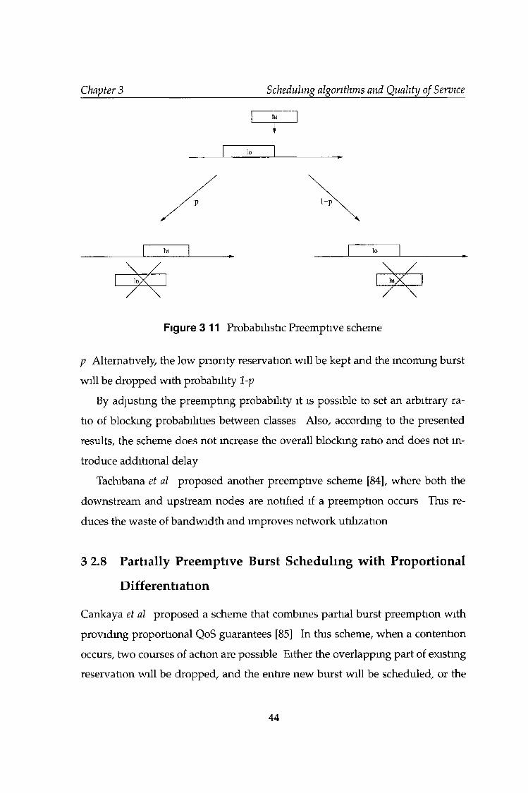
Chapter 3 Scheduling algorithms and Quality of Service
hi
Tlo
Figure 3 11 Probabilistic Preemptive scheme
p Alternatively, the low priority reservation will be kept and the incoming burst
will be dropped with probability 1-p
By adjusting the preempting probability it is possible to set an arbitrary ra
tio of blocking probabilities between classes Also, according to the presented
results, the scheme does not increase the overall blocking ratio and does not in
troduce additional delay
Tachibana et al proposed another preemptive scheme [84], where both the
downstream and upstream nodes are notified if a preemption occurs This re
duces the waste of bandwidth and improves network utilization
3 2.8 Partially Preemptive Burst Scheduling with Proportional
Differentiation
Cankaya et al proposed a scheme that combines partial burst preemption with
providing proportional QoS guarantees [85] In this scheme, when a contention
occurs, two courses of action are possible Either the overlapping part of existing
reservation will be dropped, and the entire new burst will be scheduled, or the
44
Chapter 3 Scheduling algorithms and Quality of Service
existing reservation will be left untouched and only the non-overlapping part
of the new burst will be scheduled The exact choice depends on whether the
contending bursts conform to their usage profiles The usage profiles are defined
identically as m Section 3 2 3
This QoS scheme not only provides service differentiation, but also, accord
ing to presented simulation results, improves overall burst loss probability and
utilization
3 2.9 DiffServ over Optical Burst Switching (DS-OBS)
Blake et at presented a framework for supporting IETF DiffServ [86] in Optical
Burst-Switched networks [87] In their approach an OBS edge node is combined
with a DiffServ edge router and is responsible for
• Traffic classifymg,
• DiffServ traffic conditioning,
• Burst assembly,
• Offset Management,
• Burst and control packet generation
The authors proposed a burst assembly algorithm that supports the DiffServ
services and adapts its parameters according to traffic conditions
In a core node, arriving control packets are first buffered in multiple queues,
accordmg to their class and destination Instead of scheduling them on a first
come - first served basis, the node performs priority scheduling, thus providing
differentiated service Consequentially, differentiated service is achieved for the
data bursts as well The authors claim, based on their simulation results, that
this scheme not only provides QoS differentiation, but also enhances the whole
network performance
45
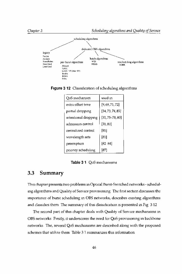
Chapter 3 Scheduling algorithms and Quality of Service
scheduling algorithms
dedicated OBS algorithms
per-burst algorithmsiioruonLAUCLA U C -VF (Mm -SV)BcstPitBORAPWA
batch algorithms WQS MSSIS
rescheduling algorithms ODBR
Figure 3 12 Classification of scheduling algorithms
QoS mechanism used in
extra offset time [9,69,71,72]
partial droppmg [34,73,74,85]
intentional dropping [31,75-78,80]
admission control [31,80]
centralized control [81]
wavelength sets [81]
preemption [82-84]
priority scheduling [87]
Table 3 1 QoS mechanisms
3.3 Sum m ary
This chapter presents two problems in Optical Burst-Switched networks - schedul
ing algorithms and Quality of Service provisioning The first section discusses the
importance of burst schedulmg m OBS networks, describes existing algorithms
and classifies them The summary of this classification is presented in Fig 3 12
The second part of this chapter deals with Quality of Service mechanisms in
OBS networks Firstly, it underscores the need for QoS provisioning in backbone
networks The, several QoS mechanisms are described along with the proposed
schemes that utilize them Table 3 1 summarizes this information
46
Chapter 4
Cost functions
In this chapter the idea of a cost function is described Firstly, the motivation is
presented, along with a formal definition of a cost function, theoretical analysis
and a proposed formula Then several possible applications of cost functions are
presented, m particular
• scheduling algorithms,
• FDL management,
• Quality of Service - intentional burst droppmg
4.1 M otivation
In Optical Burst Switched networks reservations are made in advance This, due
to differing offset times, leads to the creation of gaps or voids In other words, the
available bandwidth is being fragmented, resulting m lower bandwidth utilisa
tion and higher loss ratio Because of that, the alignment of bursts m a channel is
of a great importance
Many existing scheduling algorithms use some sort of metric to judge the suit
ability of a particular channel for a particular burst However, the decision is al
ways hard, 1 e the metric is only used to choose the best channel and is not used
elsewhere In particular, while a certain algorithm may decide that channel m is
better that channel n, it does not try to estimate the magnitude of the difference
It can be reasonably expected that the network performance can be improved
in two ways
47
Chapter 4 Cost functions
• A better type of metric (a cost function) can be designed,
• Its value can be used not only for burst scheduling, but also for other pur
poses
As will be shown in this and the following chapters, the cost function achieves
both of those goals
4.2 Definition
When any burst is allocated m any channel, it makes its bandwidth unavailable
for other bursts By doing so, it increases the probability of contention for future
bursts PB{Bm\Bn) > PB(Bm\'Bfl), for m > n, where PB{Bm\Bn) - blocking probability
for burst m, if burst n was allocated and Pg (Bm | ) - blockmg probability for burst
m, if burst n was not allocated
The cost function C() is defined as a value that is an indicator of the probabil
ity of future contention, caused by allocating a particular burst in a particular
channel C(Bn) ~ PB(Bx\Bn)
4.3 Cost function form ulas
The state of a channel can be described by a set of reservations Each reservation
consists of its starting time and ending tame If we denote the starting time of the
l-th reservation by S, and its ending time by El then the state of the entire channel
can be represented by vectors S = [Si,52, ,Sn]and E =[E\,Ei, ,En] where n is
the number of reservations The newly arriving burst is described by its starting
and ending times, S and E, respectively
The cost function is defined m relation to the channel state, the new burst and
possibly other variables
C = f(S ,E ,S ,E , )
48
( 4 1 )
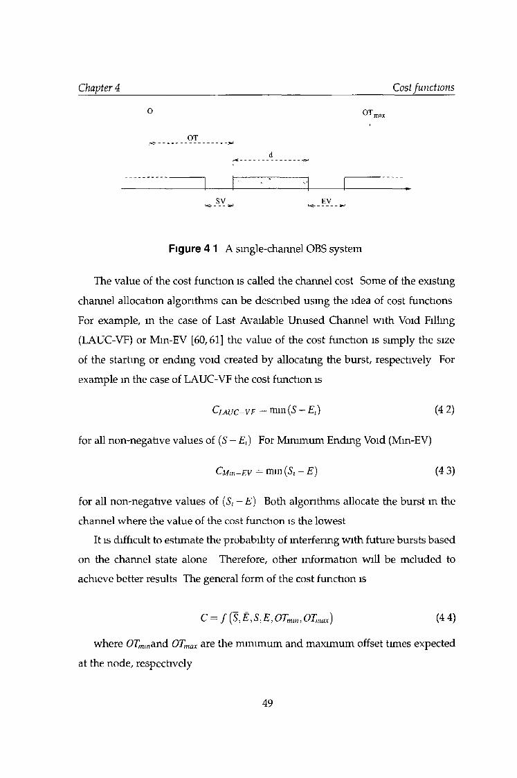
Chapter 4 Cost functions
OT,
OT
sv EVL<------
Figure 4 1 A single-channel OBS system
The value of the cost function is called the channel cost Some of the existing
channel allocation algorithms can be described usmg the idea of cost functions
For example, in the case of Last Available Unused Channel with Void Filling
(LAUC-VF) or Min-EV [60,61] the value of the cost function is simply the size
of the starting or ending void created by allocating the burst, respectively For
example in the case of LAUC-VF the cost function is
C l a u c - v f = mm (S - Et) (4 2)
for all non-negative values of ( S - E t) For Minimum Endmg Void (Min-EV)
Cmiu- ev — nun (St ~ E ) (4 3)
for all non-negative values of (St - E) Both algorithms allocate the burst m the
channel where the value of the cost function is the lowest
It is difficult to estimate the probability of interfering with future bursts based
on the channel state alone Therefore, other information will be mcluded to
achieve better results The general form of the cost function is
c = f ( S , £ 1s ,E ,o r mm,a r max) (44)
where OTmmand OTmax are the minimum and maximum offset times expected
at the node, respectively
49
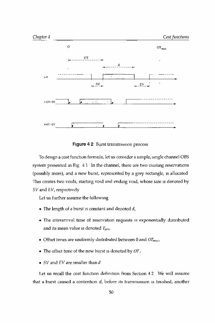
Chapter 4 Cost functions
OT,
OT
t=0
sv---- EVi<_------
t=OT-SV k____
t>OT~SV
Figure 4 2 Burst transmission process
To design a cost function formula, let us consider a simple, single channel OBS
system presented in Fig 4 1 In the channel, there are two existing reservations
(possibly more), and a new burst, represented by a grey rectangle, is allocated
This creates two voids, startmg void and ending void, whose size is denoted by
SV and EV, respectively
Let us further assume the following
• The length of a burst is constant and denoted d,
• The interarrival time of reservation requests is exponentially distributed
and its mean value is denoted Tarr,
• Offset times are uniformly distributed between 0 and OTmax,
• The offset time of the new burst is denoted by OT,
• SV and EV are smaller than d
Let us recall the cost function definition from Section 4 2 We will assume
that a burst caused a contention if, before its transmission is finished, another
50
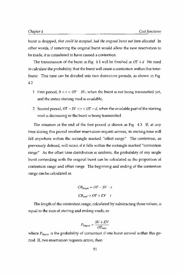
Chapter 4 Cost functions
burst is dropped, that could be accepted, had the original burst not been allocated In
other words, if removing the original burst would allow the new reservation to
be made, it is considered to have caused a contention
The transmission of the burst in Fig 4 1 will be finished in O T + d We need
to calculate the probability that the burst will cause a contention within this time
frame This time can be divided into two distinctive periods, as shown in Fig
42
1 First period, 0 < t < OT - S V , when the burst is not being transmitted yet,
and the entire starting void is available,
2 Second period, O T - SV < t < O T +d, when the available part of the starting
void is decreasing or the burst is being transmitted
The situation at the end of the first period is shown in Fig 4 3 If, at any
time during this period another reservation request arrives, its starting time will
fall anywhere within the rectangle marked "offset range" The contention, as
previously defined, will occur, if it falls within the rectangle marked "contention
range" As the offset time distribution is uniform, the probability of any single
burst contending with the original burst can be calculated as the proportion of
contention range and offset range The beginning and endmg of the contention
range can be calculated as
CRbtgm = OT — SV — t
CRend — OT + EV — t
The length of the contention range, calculated by substracting those values, is
equal to the sum of starting and ending voids, so
SV + EVM burst fyp
maxwhere P\ burst is the probability of contention if one burst arrived within this pe
riod If, two reservation requests arrive, then
51
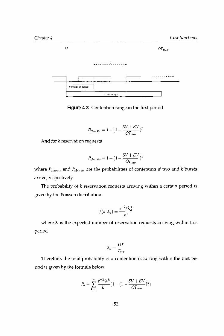
Chapter 4 Cost functions
o OT,
contention range
offset range
Figure 4 3 Contention range in the first period
And for k reservation requests
Pkbursts — 1 (1
OTn
SV + E V )k OTmax
where Pibursts and Pkbursts are the probabilities of contention if two and k bursts
arrive, respectively
The probability of k reservation requests arriving within a certain period is
given by the Poisson distribution
f ( k K ) = — ^
where X is the expected number of reservation requests arriving within this
period
Xa —OT
Therefore, the total probability of a contention occurring within the first pe
riod is given by the formula below
k- 1
SV + EV k OTmay ’ ’
52
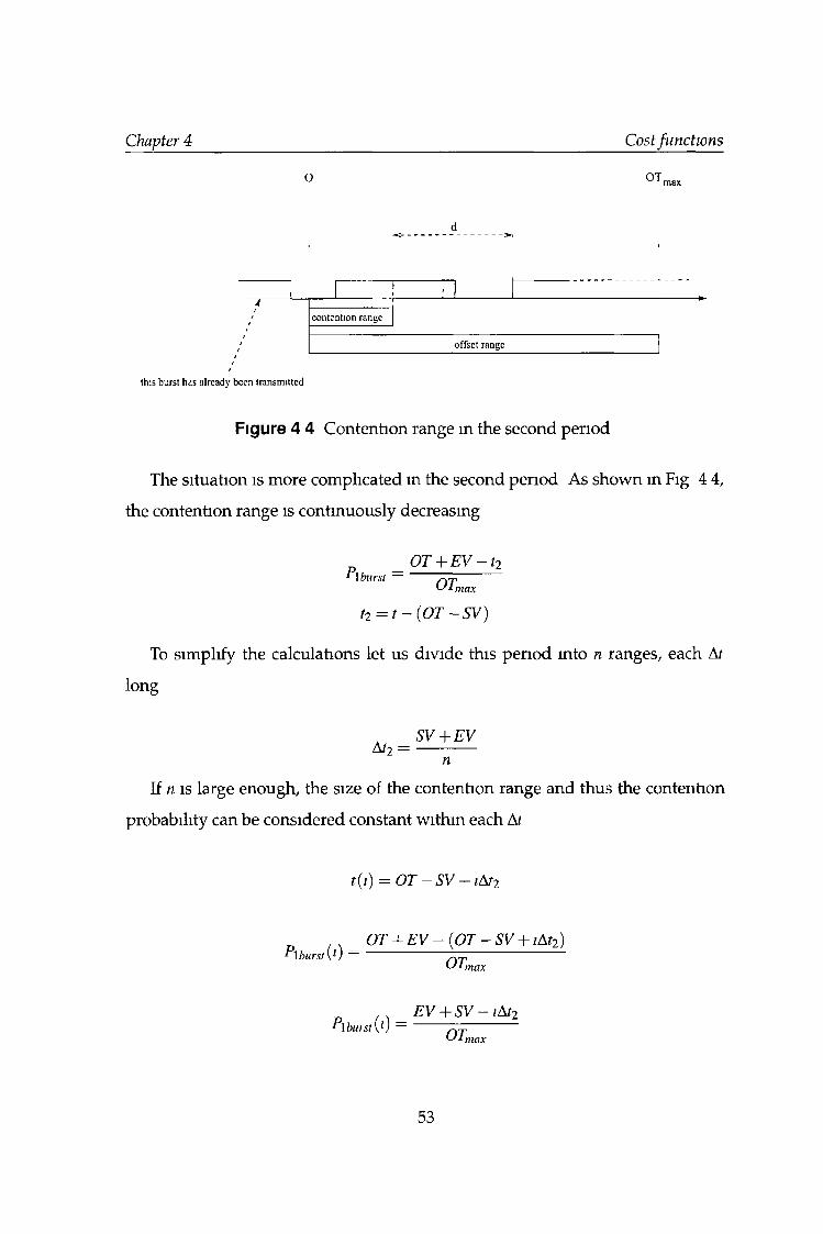
Chapter 4 Cost functions
o OT.
4///t///
contention range
offset range
this burst has already been transmitted
Figure 4 4 Contention range in the second period
The situation is more complicated m the second period As shown in Fig 4 4,
the contention range is continuously decreasing
burstOT + E V -Î2
OTmax
t2 = t-{or-sv)To simplify the calculations let us divide this period into n ranges, each At
long
àt2 —SV + E V
If n is large enough, the size of the contention range and thus the contention
probability can be considered constant within each At
t(i) = OT — SV + iAt2
OT + EV — (OT — SV + iAt2)P \burs t( l ) —
P\ bu>st(l) —
OT)nax
EV + S V - iA t2O T m n r
53
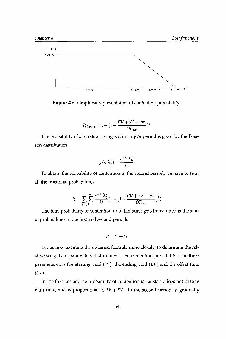
Chapter 4 Cost functions
Figure 4 5 Graphical representation of contention probability
kburstsEV + S V - iA t2 k
OTmax
The probability of k bursts arriving within any At period is given by the Pois
son distribution
f (k Xb)k'
To obtain the probability of contention in the second period, we have to sum
all the fractional probabilities
h * EV + S V -iA r2
1=0 k = \ K max
The total probability of contention until the burst gets transmitted is the sum
of probabilities in the first and second periods
P = P a + P b
Let us now examine the obtained formula more closely, to determme the rel
ative weights of parameters that influence the contention probability The three
parameters are the starting void (5V), the ending void (EV) and the offset time
(OT)
In the first period, the probability of contention is constant, does not change
with time, and is proportional to SV + EV In the second period, it gradually
54

Chapter 4 Cost functions
decreases to 0, as shown in Fig 4 5 The total probability of contention is repre
sented by the area under the curve This area can be expressed as a function of
SV, EV and OT Then, in order to determine the relative weights of starting and
ending voids, the obtained formula is differentiated with respest to S and EV
dP = OT — SVdSVdP
= OT + EVdEV
It is apparent that, for very small offset times, the influence of the starting
void decreases to 0 (the starting void cannot be smaller than the offset time, so
O T - S V ^ 0) This leads us to the conclusion that for small offset time the endmg
void will be more important than the startmg void, and for large offset times the
difference will be negligible
For example, the size of the startmg void does not matter if the burst arrived
with the smallest possible offset time No other burst will be allocated in this gap
anyway Therefore, the proposed cost function first calculates the channel price
according to LAUC-VF and Min-EV, then applies appropriate weights to those
results and chooses the smaller value
„ ( C lA U C ~ V F C m ih -E V \ (AC = nun --------------, --------------- (4 5)\ O T - O T mir; O T max~ O T ) V '
This formula reflects the relative weights of SV and EV, depending on the off
set time However it does nor approximate the previously derived probabilities
in a strict sense
The average value of the cost function as presented above depends on the
average void size which, in turn, depends on the link load In some cost func
tion applications (m particular the intentional burst droppmg, described later in
this chapter) it is desirable to reduce the dependence of the average cost function
value on the load This can be achieved by multiplying the void sizes by the link
load
55
Chapter 4 Cost functions
~ ( C lA U C -V F C miti-E V \ T tA~ nUn \ O T — 0 T mm ’ 0 T max — O T ) ,mk
where Liinit is the link load at a given time, as a fraction of maximum link load
4.4 A pplications of a cost function
A cost function gives us the knowledge about the quality of the alignment of a
given burst with other bursts It can be seen as an imaginary cost of using a par
ticular channel for this burst This section explams how this information can be
used to improve the performance of OBS networks A cost-based scheduling al
gorithm will be presented in Section 4 41 and in Section 4 4 2 it will be explained
how a cost function can be used to match the size of an FDL bank with the needs
of a node Finally, in Section 4 4 3 a cost-based burst dropping algorithm will be
presented
4.4 1 Scheduling algorithms
Let us imagine an OBS node Certam sets of resources will be contained within
this node Examples of such resources are
• outgoing links,
• wavelength converters,
• Fiber Delay Lmes
When a reservation request for an incoming burst arrives at the node, it will
use some or all of those resources For example, the burst may be forwarded on
the same wavelength, it may also be converted to another wavelength an d /o r
delayed m an FDL Frequently, there is more than one way of handling a burst A
contention may be resolved by wavelength change, buffering or both
56
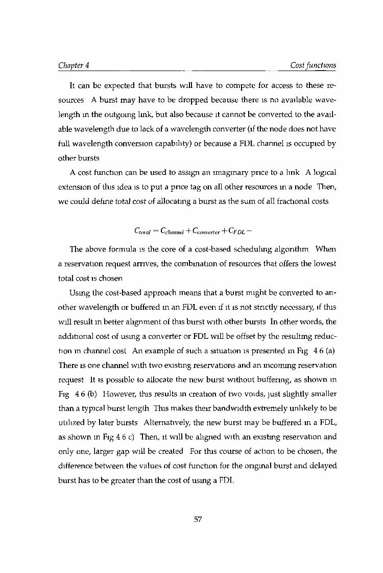
Chapter 4 Cost functions
It can be expected that bursts will have to compete for access to these re
sources A burst may have to be dropped because there is no available wave
length m the outgoing link, but also because it cannot be converted to the avail
able wavelength due to lack of a wavelength converter (if the node does not have
full wavelength conversion capability) or because a FDL channel is occupied by
other bursts
A cost function can be used to assign an imaginary price to a link A logical
extension of this idea is to put a price tag on all other resources in a node Then,
we could define total cost of allocating a burst as the sum of all fractional costs
Ctotal = Cchannel “t" Cconverter 4" C f d L
The above formula is the core of a cost-based scheduling algorithm When
a reservation request arrives, the combination of resources that offers the lowest
total cost is chosen
Using the cost-based approach means that a burst might be converted to an
other wavelength or buffered in an FDL even if it is not strictly necessary, if this
will result in better alignment of this burst with other bursts In other words, the
additional cost of using a converter or FDL will be offset by the resultmg reduc
tion m channel cost An example of such a situation is presented in Fig 4 6 (a)
There is one channel with two existing reservations and an incoming reservation
request It is possible to allocate the new burst without buffering, as shown in
Fig 4 6 (b) However, this results in creation of two voids, just slightly smaller
than a typical burst length This makes their bandwidth extremely unlikely to be
utilized by later bursts Alternatively, the new burst may be buffered in a FDL,
as shown in Fig 4 6 c) Then, it will be aligned with an existing reservation and
only one, larger gap will be created For this course of action to be chosen, the
difference between the values of cost function for the original burst and delayed
burst has to be greater than the cost of usmg a FDL
57
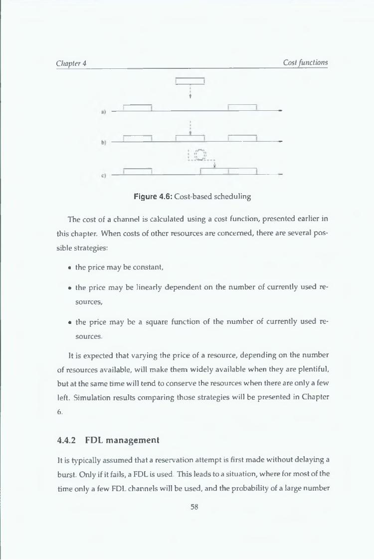
Chapter 4 Cost functions
♦
Figure 4.6: Cost-based scheduling
The cost of a channel is calculated using a cost function, presented earlier in
this chapter. When costs of other resources are concerned, there are several pos
sible strategies:
• the price may be constant,
• the price may be linearly dependent on the number of currently used re
sources,
• the price may be a square function of the number of currently used re
sources.
It is expected that varying the price of a resource, depending on the number
of resources available, will make them widely available when they are plentiful,
but at the same time will tend to conserve the resources when there are only a few
left. Simulation results comparing those strategies will be presented in Chapter
6 .
4.4.2 FDL m anagem ent
It is typically assumed that a reservation attempt is first made without delaying a
burst. Only if it fails, a FDL is used. This leads to a situation, where for most of the
time only a few FDL channels will be used, and the probability of a large number
58
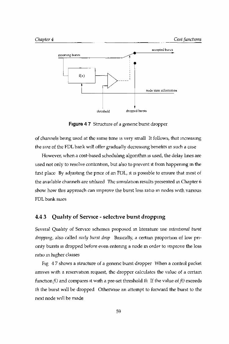
Chapter 4 Cost functions
accepted bursts
Figure 4 7 Structure of a generic burst dropper
of channels being used at the same time is very small It follows, that increasing
the size of the FDL bank will offer gradually decreasing benefits in such a case
However, when a cost-based schedulmg algorithm is used, the delay lines are
used not only to resolve contention, but also to prevent it from happening m the
first place By adjusting the price of an FDL, it is possible to ensure that most of
the available channels are utilized The simulation results presented m Chapter 6
show how this approach can improve the burst loss ratio m nodes with various
FDL bank sizes
4.4 3 Q uality of Service - selective b u rs t d ropp ing
Several Quality of Service schemes proposed m literature use intentional burst
dropping, also called early burst drop Basically, a certam proportion of low pri
ority bursts is dropped before even entering a node in order to improve the loss
ratio m higher classes
Fig 4 7 shows a structure of a generic burst dropper When a control packet
arrives with a reservation request, the dropper calculates the value of a certain
functionf() and compares it with a pre-set threshold th If the value o f/0 exceeds
th the burst will be dropped Otherwise an attempt to forward the burst to the
next node will be made
59
Chapter 4 Cost functions
Burst dropper can be
• Random, when the value of function/0 is obtained from a random number
generator [76-79],
• Deterministic, if for example f(SEQ) = SEQ mod 20, where SEQ - sequence
number of incoming burst, or if all bursts belonging to a certam class are
dropped [31,80],
• Cost-based, if f() is a cost function
The value of a cost function reflects the amount of resources within a node
that are needed to forward the burst It is also an indicator of the probability
that acceptmg this burst will cause contention in the future Therefore, droppmg
only those bursts with cost function values above a certam threshold can be ex
pected to offer better performance than droppmg the same percentage of bursts
randomly
4.5 Sum m ary
In this chapter the idea of a cost function was presented Cost function is an in
dicator of the probability of the future contention caused by allocating a certam
burst Therefore, its value can be considered to be an imaginary cost of usmg the
channel
Several applications of a cost function have been proposed
• Scheduling algorithms - the value of a cost function along with the cost of
other resources (like FDLs) is considered to be the total cost of allocating a
burst, and the lowest-priced combmation is chosen,
• FDL management - when a cost-based scheduling algorithm is used, it is
possible to effectively utilize FDL banks of arbitrary, especially large sizes,
60

• Quality of Service - if a QoS scheme uses intentional burst dropping, then a
cost-based algorithm, where only those bursts with the cost function value
above a certam threshold are dropped, offers better overall performance
than a random one
Chapter 4 Cost functions
61
Chapter 5
Simulator
Several analytical models of Optical Burst-Switched networks have been pre
sented (e g [72,88,89]) However m many cases such analysis is difficult or im
possible Therefore, it was necessary to develop a suitable simulator to test the
ideas presented in this thesis This chapter describes the structure of this simula
tor, discusses the choices that had to be made and provides its short usage manual
and a few example scripts
5.1 Existing OBS sim ulation program s
Optical Burst Switching is a rather new paradigm, and there are relatively few
simulators available The non-commercial tools include
• Optical WDM Network Simulator (OWns) has been developed by B Wen
et al at the University of Maryland DAWN lab [90] It is a WDM extension
to the ns-2 simulator Its later versions allow to simulate OBS networks as
well
• OBS-ns simulator, developed at WINE laboratory (Information and Com
munications University, Taejeon, Korea) is based on the OWns simulator
• Also, many stand-alone simulators are mentioned in the literature [91,92],
but are not made publicly available
62
Chapter 5 Simulator
5.2 Stand-alone sim ulator vs. extension to an existing
sim ulator
When a simulation program with desired capabilities does not exist, it is neces
sary to develop a new simulator. The first choice that has to be made is whether to
develop one from scratch or extend/m odify an existing simulator. The answer is
non-obvious and depends on particular circumstances and desired characteristics
of the final program.
If a completely new simulator is written, it is likely to be well-suited for the
intended purpose and fast. Unfortunately, it will also be rather inflexible, and
any serious changes to it will require much effort. Also, this approach might be
time-consuming, as the entire simulator core has to be developed from scratch.
Extending an existing simulator has many advantages. First of all, the simu
lator core and user interface are already in place. Their functionality is likely to
have already been validated. Also, in case of OBS simulator, it is useful to have a
TCP/IP-capable simulator in place. However, a significant amount of time may
be needed to get to know the simulator's internals in order to extend it.
Keeping all of the above in mind, 1 decided to extend the well-known ms-2
simulator. This extension will be described in Section 5.4.
5.3 Ns-2 sim ulator
Ns-2 is a discrete event network simulator [93]. It is mainly intended as a tool
to investigate TCP/IP based wired and wireless networks. A wide range of TCP
variants, routing protocols and traffic sources are supported.
Ns-2 uses a tivo language concept [94]. OTcl scripting language is used as a
frontend to C++ based simulator core. This solution offers the best features of an
interpreted language (ease of development and modification, interactivity) with
those of a compiled language (speed, efficiency).
63
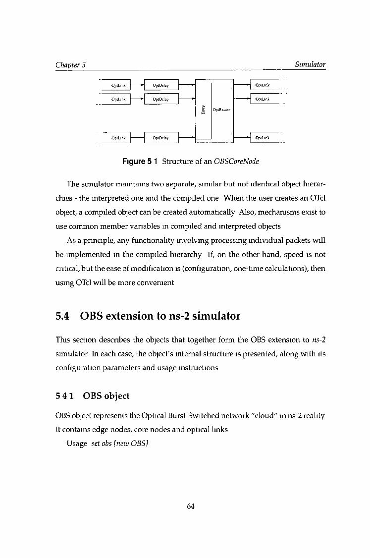
Chapter 5 Simulator
Figure 5 1 Structure of an OBSCoreNode
The simulator maintains two separate, similar but not identical object hierar
chies - the interpreted one and the compiled one When the user creates an OTcl
object, a compiled object can be created automatically Also, mechamsms exist to
use common member variables in compiled and interpreted objects
As a principle, any functionality involving processmg individual packets will
be implemented in the compiled hierarchy If, on the other hand, speed is not
critical, but the ease of modification is (configuration, one-time calculations), then
using OTcl will be more convenient
5.4 OBS extension to ns-2 sim ulator
This section describes the objects that together form the OBS extension to ns-2
simulator In each case, the object's internal structure is presented, along with its
configuration parameters and usage instructions
5 4 1 OBS object
OBS object represents the Optical Burst-Switched network "cloud" m ns-2 reality
It contains edge nodes, core nodes and optical lmks
Usage set obs [new OBS]
64
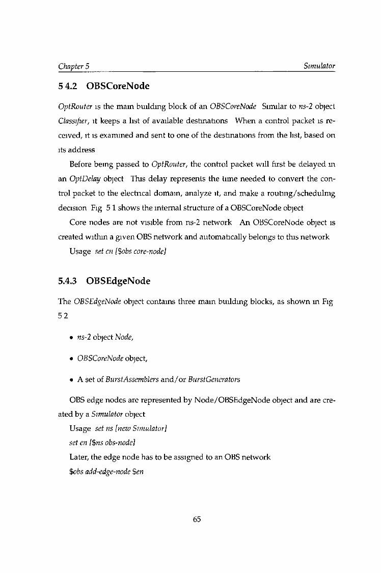
Chapter 5 Simulator
5 4.2 OBSCoreNode
OptRouter is the mam building block of an OBSCoreNode Similar to ns-2 object
Classifier, it keeps a list of available destinations When a control packet is re
ceived, it is examined and sent to one of the destinations from the list, based on
its address
Before bemg passed to OptRouter, the control packet will first be delayed in
an OptDelay object This delay represents the time needed to convert the con
trol packet to the electrical domain, analyze it, and make a routing/schedulm g
decision Fig 5 1 shows the internal structure of a OBSCoreNode object
Core nodes are not visible from ns-2 network An OBSCoreNode object is
created within a given OBS network and automatically belongs to this network
Usage set cn [$obs cor e-node]
5.4.3 OBSEdgeNode
The OBSEdgeNode object contains three mam building blocks, as shown in Fig
52
• ns-2 object Node,
• OBSCoreNode object,
• A set of BurstAssemblers an d /o r BurstGenerators
OBS edge nodes are represented by Node/OBSEdgeNode object and are cre
ated by a Simulator object
Usage set ns [new Simulator]
set en [$ns obs-node]
Later, the edge node has to be assigned to an OBS network
$obs add-edge-node $en
65
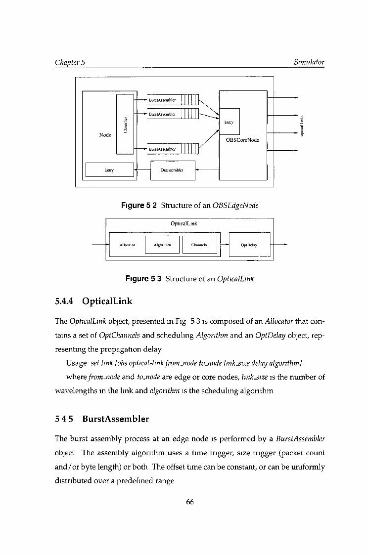
Chapter 5 Simulator
Figure 5 2 Structure of an OBSEdgeNode
OpticalLink
Allocator Algorithm Channels OptDclay
Figure 5 3 Structure of an OpticalLink
5.4.4 O pticalL ink
The OpticalLink object, presented in Fig 5 3 is composed of an Allocator that con
tains a set of OptChannels and scheduling Algorithm and an OptDelay object, rep
resenting the propagation delay
Usage set link [obs optical-hnkfromjiode tojiode hnksize delay algorithm]
where from -node and tojiode are edge or core nodes, link s ize is the number of
wavelengths in the link and algorithm is the scheduling algorithm
5 4 5 B urstA ssem bler
The burst assembly process at an edge node is performed by a BurstAssembler
object The assembly algorithm uses a time trigger, size trigger (packet count
an d /o r byte length) or both The offset time can be constant, or can be uniformly
distributed over a predefined range
66
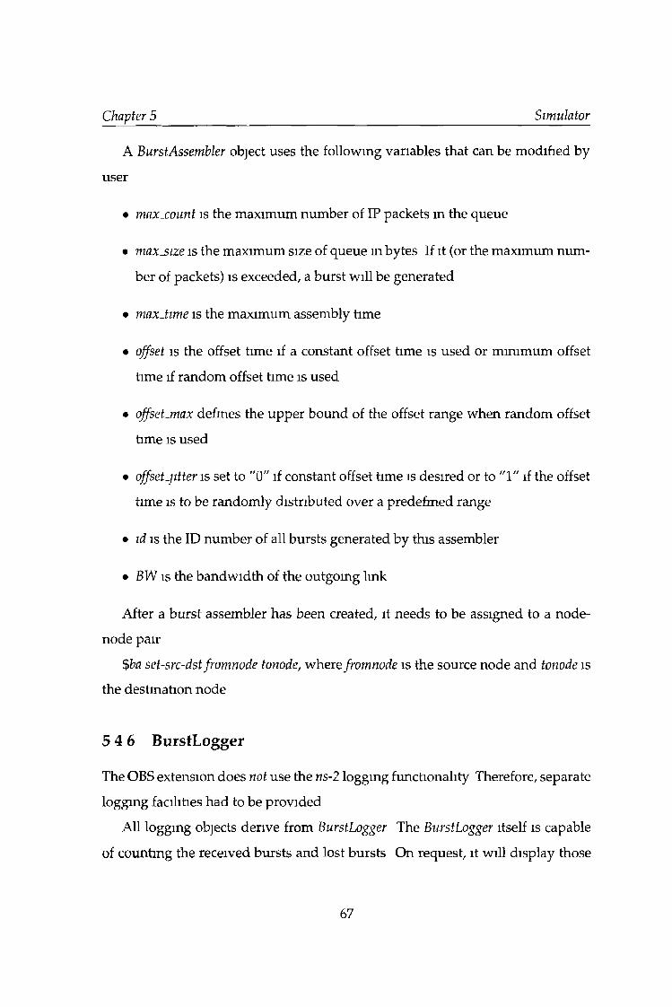
Chapter 5 Simulator
A BurstAssembler object uses the following variables that can be modified by
user
• maxxount is the maximum number of IP packets in the queue
• max size is the maximum size of queue m bytes If it (or the maximum num
ber of packets) is exceeded, a burst will be generated
• max.time is the maximum assembly time
• offset is the offset time if a constant offset time is used or mmimum offset
time if random offset time is used
• offset-max defmes the upper bound of the offset range when random offset
time is used
• off set.jitter is set to "0" if constant offset time is desired or to "1" if the offset
time is to be randomly distributed over a predefmed range
• id is the ID number of all bursts generated by this assembler
• BW is the bandwidth of the outgoing link
After a burst assembler has been created, it needs to be assigned to a node
node pair
$ba set-src-dst fromnode tonode, where fromnode is the source node and tonode is
the destination node
5 4 6 BurstLogger
The OBS extension does not use the ns-2 logging functionality Therefore, separate
logging facilities had to be provided
All logging objects derive from BurstLogger The BurstLogger itself is capable
of counting the received bursts and lost bursts On request, it will display those
67
Chapter 5 Simulator
number along with the loss ratio, or write them to a specified file It can also filter
the incoming bursts accordmg to their source, destination, and ID
Each BurstLogger implements the following commands
• $bl set’src source .address - only bursts with this source address will be taken
mto account,
• $bl set-dst destination jxddress - only bursts with this destination address will
be taken mto account,
• $bl set-id burst JD - only bursts with this ID will be taken mto account,
-1 is considered to be a wildcard and will match any source address, destina
tion address and burst ID For example, if src = 10, d s t = - 1 and ID — —1, then
all bursts with a source address of 10 will be logged, regardless of their ID and
destination address
Other logging objects are
• BurstLogger[Distribution calculates the distribution of burst length as the
function of mterarnval time and vice versa
• BurstLogger[LossDistnbution in addition to measuring the burst loss ratio,
measures the loss distribution, e g the loss probability as a function of burst
length
• BurstLogger/Time averages the traffic m a desired mterval and writes the re
sults to a file
• BurstLogger/Traffic calculates the total load within the simulation time
• BurstLogger/Trace logs every received burst to a file
A BurstLogger or any of its subclasses can be added to the following network
components, each of which implements an add-logger command
68
Chapter 5 Simulator
• OpticalLink A BurstLogger will track traffic characteristics and loss ratio in
this particular link
• BurstAssembler and its derivative objects A BurstLogger added to a BurstAssem-
bler can be used to analyze traffic characteristics However, no loss ratio will
be reported as no bursts can be lost within a burst assembler
• OBSEdgeNode A BurstLogger can be used to analyze the traffic received by
an edge node
An arbitrary number of BurstLoggers can be added to a network component
This is useful when different classes of bursts have to be tracked separately
5.5 Traffic sources
Using ns-2 based IP traffic sources and burst assembly can be very realistic How
ever, as each burst may contain hundreds of packets, this approach is also time
consuming Therefore, m many cases it is beneficial to use a burst generator in
stead of a burst assembler As long as statistical properties of generated traffic
match those of assembled traffic, the simulations will yield proper results m much
shorter time
The OBS extension to ns-2 provides several objects that can be used to generate
burst traffic Each of those objects extends the BurstAssembler class shares much of
its functionality In particular the offset, offset jnax and offset .jitter variables need
to be set Also, the set-src-dst procedure needs to be called
All burst generator objects also define procedures start and stop, used to start
and stop the generation process, respectively
5 5.1 B urstA ssem bler/Exponential
Burst Assembler/Exponential generates traffic where both burst length and mterar-
nval time are exponentially distributed This type of traffic is characteristic for
69
Chapter 5 Simulator
telephony networks and therefore well-studied Although it does not perfectly
approximate the properties of assembled IP traffic, many authors use it in their
simulations [9,23,88] Also, it is useful for simulator validation as it can be rela
tively easily studied analytically
In addition to those inherited from BurstAssembler this generator defines the
following variables
• avlength is the average length of a burst in seconds
• load is the desired load m Erlangs
• const length is set to "0" if the burst length is to be exponentially distributed
or to "1" if it is to be constant
5.5.2 B urstA ssem bler/G enerator
By analyzing the functioning of a burst assembler it can be noted than the burst
length and its assembly time are, m fact, dependent For example, if the assembly
time is shorter than the maximum value, then it it obvious that it was the length
trigger that caused the burst to be generated, and the burst will be of the maxi
mum length Conversely, maximum burst size implies that the particular burst
generation was triggered by exceeding the maximum assembly time
Those dependencies can be described by correlated or conditional distribu
tions Conditional distribution is a function of two arguments, the first one be
ing the value of the previously generated assembly time or burst length It can
be viewed as a set of distributions - the previously generated value determmes
which distribution is to be used next [95]
The conditional distributions to use with this generator can be obtained by
usmg IP traffic assembled using a desired algorithm and BurstLogger[Distribution
The following methods are available
• load-aA-disti ibut ions file jriame
70
Chapter 5 Simulator
• load-l-a-distributions filejtam e
Also, the member variable correlated can be set to "0" if burst lengths and as
sembly times are to be generated independent of each other, or to if condi
tional distributions are to be used.
5.5.3 B urstA ssem bler/EnvelopeG enerator
In some simulations, it is desirable to use traffic that exhibits self-similarity and
long-range dependence. Using an appropriate IP traffic source and assembling
its traffic is not always suitable, mainly for performance reasons. The burst gen
eration itself would consume significant part of sim ulator's time.
Envelope generator, is a new type of burst generator that can efficiently generate
long-range dependent traffic. It exploits the fact that the process of assembling
IP packets into bursts is similar to calculating bandwidth within the assembly
window. Therefore, if the bandwidth at any time can be known, the process of
generating and assembling IP packets can be skipped altogether.
In this traffic source, a set of Pareto-distributed on /off sources is used. No IP
packets are generated, however. Instead, the state of each source is used to calcu
late bandwidth envelope. Immediately after a burst is generated, the envelope is
sampled, and its value is used to decide when the next burst will be generated,
and what will its length be. In effect, much less simulator events are necessary to
generate a burst.
The generation process is presented in Fig. 5.4. There are three on/off sources.
The rectangles on the corresponding axes represent IP packets that would nor
mally be generated. In an envelope generator, however, the sources only report
their state when pooled. This information is then used to calculate bandwidth
envelope, shown below. Its value determines the size of the next burst and the
simulated assembly time. The same principle can be used to generate a different
type of traffic - for example, exponentially distributed on/off sources can be used.
71
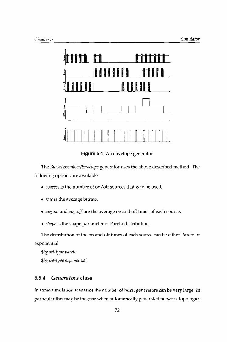
Chapter 5 Simulator
Hill rtttnr
Figure 5 4 An envelope generator
The Bui stAssembler[Envelope generator uses the above described method The
following options are available
• sources is the number of on/off sources that is to be used,
• rate is the average bitrate,
• avgxn and avgjoff are the average on and off times of each source,
• shape is the shape parameter of Pareto distribution
The distribution of the on and off times of each source can be either Pareto or
exponential
set-type pareto
$bg set-type exponential
5.5 4 Generators class
In some simulation scenarios the number of burst generators can be very large In
particular this may be the case when automatically generated network topologies
72
Chapter 5 Simulator
are used This makes starting and stopping each burst generator individually dif
ficult and impractical Generatois is a helper object used to simplify management
of many burst generators
The class Generators defines the following methods
• add~generator adds a generator to the object,
• start starts all generators,
• stop stops all generators
5.6 Scheduling algorithm s
When creating an OpticalLink, the user has to specify the scheduling algorithm
that is to be used The OBS simulator offers the following scheduling algorithms
• Algorithm /FirstFit,
• Algorithm/RoundRobin,
• Algorithm/MostUsed,
• Algonthm/LeastUsed,
• Algorithm/Random,
• Algorithm /LAUC-VF,
• Algorithm /Mm-EV,
• Algorithm /GapFilling
All of the above algorithms except GapFilling are described in detail in Chapter
3 They also do not require any additional configuration
GapFilling is a cost-based algorithm, using as a metric either one of the cost
functions proposed in Chapter 4 It defines the following variables which need to
be set before creating the link
73
Chapter 5 Simulator
• miri-offset is the minimum offset that is expected at the node,
• maxjoffset is the maximum offset expected at the node,
• fdLpnce is the base price of an FDL, if FDLs are used
5.7 Burst dropping
A burst dropping technique, described in Section 3 2 3 and Section 4 4 2 can be
implemented by using a BurstDropper object There are two types of a burst drop
per available
• BurstDropper/Random discards bursts m a random fashion,
• BurstDropper/Cost drops a burst when its cost function value exceeds a cer
tain threshold
A BurstDropper can be configured to only drop certam bursts This is done
using the same syntax as in case of a BurstLogger
• set-src
• set-dst
• set-id
The default value of source, destination and ID are -1, which means that all
bursts can be dropped
The proportion of dropped bursts is determined by setting the variable thresh
old In case of a random dropper it can be set to any value between 0 (no burst
is dropped) to 1 (all bursts are dropped) When a cost-based dropper is used, the
burst will be dropped if the value of a cost function exceeds the threshold value
74
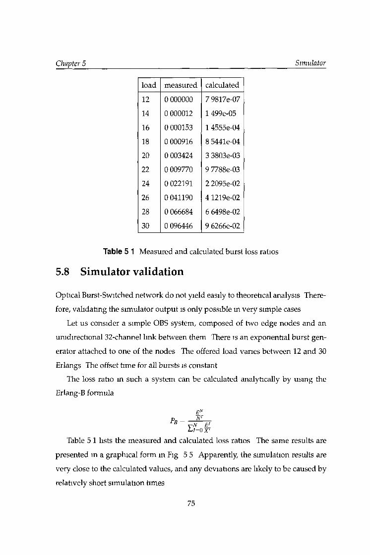
Chapter 5 Simulator
load measured calculated
12 0 000000 7 9817e-07
14 0 000012 1 499e-05
16 0 000153 1 4555e-04
18 0 000916 8 5441e-04
20 0 003424 3 3803e-03
22 0 009770 9 7788e-03
24 0 022191 2 2095e-02
26 0 041190 4 1219e-02
28 0 066684 6 6498e-02
30 0 096446 9 6266e-02
Table 5 1 Measured and calculated burst loss ratios
5.8 Sim ulator validation
Optical Burst-Switched network do not yield easily to theoretical analysis There
fore, validating the simulator output is only possible m very simple cases
Let us consider a simple OBS system, composed of two edge nodes and an
unidirectional 32-channel link between them There is an exponential burst gen
erator attached to one of the nodes The offered load varies between 12 and 30
Erlangs The offset time for all bursts is constant
The loss ratio in such a system can be calculated analytically by using the
Erlang-B formula
FNP = w Pb v n e '
L i =o x '
Table 5 1 lists the measured and calculated loss ratios The same results are
presented m a graphical form in Fig 5 5 Apparently, the simulation results are
very close to the calculated values, and any deviations are likely to be caused by
relatively short simulation times
75

Chapter 5 Simulator
Figure 5 5 Measured and calculated burst loss ratios
5.9 Routing
The problem of routing m the OBS extension can be divided into two parts
Firstly, whatever routmg scheme is supported by the IP part of the network has
to be supported Then, routmg functionality has to be provided withmg the OBS
network
5.9 1 IP routing
In ns-2 simulator, routing tables are calculated based on connection tables This
capability needs to be preserved, so that IP nodes can communicate usmg the
OBS network In order to achieve that, a PsendoLink is created between each pair
of edge nodes within a given OBS network A PseudoLink is seen by ns-2 as an
ordinary link, and thus will be used when populating the routing tables, but does
not provide any connection capabilities The entry pomt of a PseudoLink relays all
IP packets to an appropriate BurstAssembler
Fig 5 6 shows how PseudoLinks "connect" OBS edge nodes Note that this is
independent on the actual topology of the OBS network
76
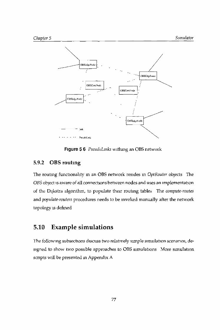
Chapter 5 Simulator
link
PscudoLink
Figure 5 6 PseudoLinks withing an OBS network
5.9.2 OBS rou ting
The routing functionality in an OBS network resides in OptRouter objects The
OBS object is aware of all connections between nodes and uses an implementation
of the Dijkstra algorithm, to populate their routing tables The compute-routes
and populate-routers procedures needs to be mvoked manually after the network
topology is defmed
5.10 Example sim ulations
The following subsections discuss two relatively simple simulation scenarios, de
signed to show two possible approaches to OBS simulations More simulation
scripts will be presented m Appendix A
77
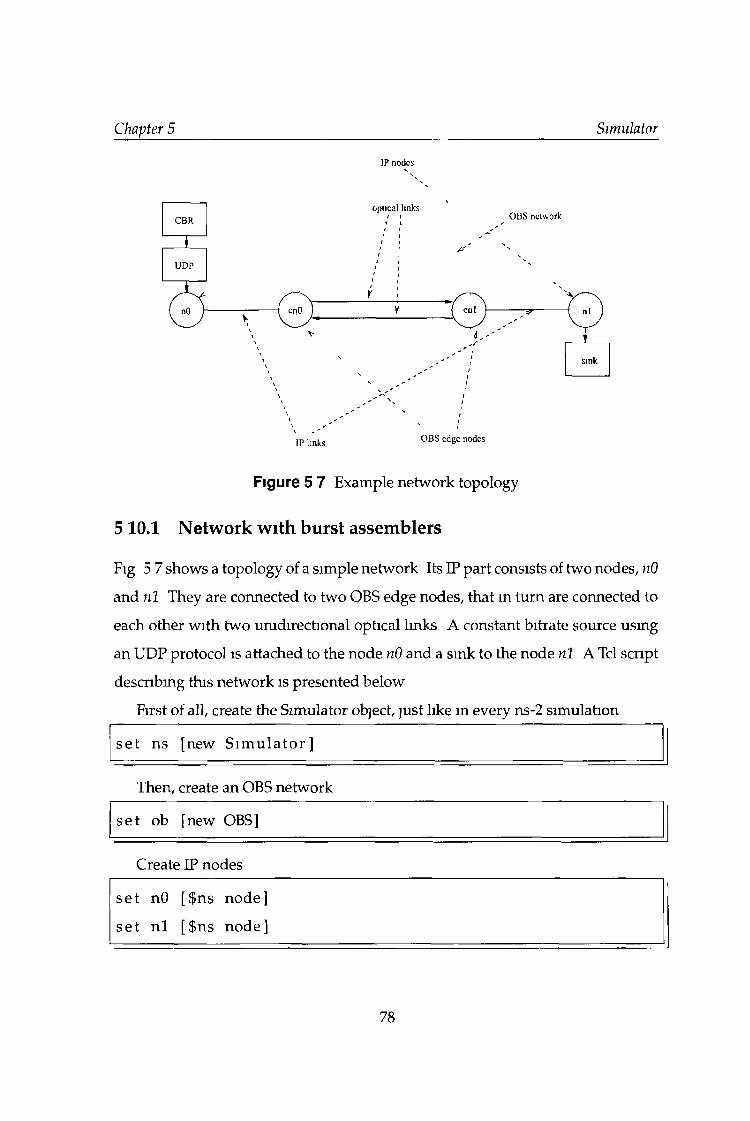
Chapter 5 Simulator
IP nodes
IP links OBS edge nodes
Figure 5 7 Example network topology
5 10.1 N etw ork w ith b u rs t assem blers
Fig 5 7 shows a topology of a simple network Its IP part consists of two nodes, nO
and n l They are connected to two OBS edge nodes, that in turn are connected to
each other with two unidirectional optical links A constant bitrate source using
an UDP protocol is attached to the node nO and a sink to the node n l A Tel script
describing this network is presented below
First of all, create the Simulator object, just like in every ns-2 simulation
s e t ns [new S im u la to r]
Then, create an OBS network
s e t ob [new OBS]
Create IP nodes
s e t nO [$ns node]
s e t n l [$ns node]
78
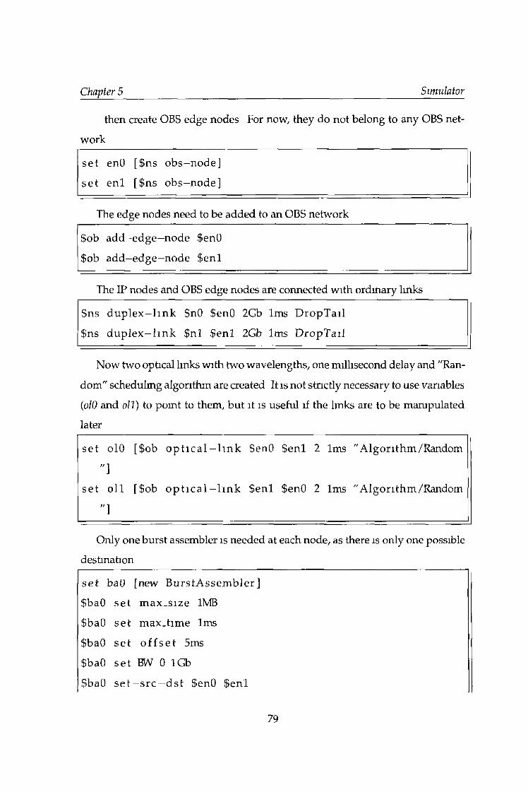
Chapter 5 Simulator
then create OBS edge nodes For now, they do not belong to any OBS net
work
s e t enO [$ns o b s-n o d e ]
s e t e n l [$ns obs—node]
The edge nodes need to be added to an OBS network
$ob a d d -e d g e -n o d e $enO
$ob ad d -e d g e -n o d e $ en l
The IP nodes and OBS edge nodes are connected with ordinary links
$ns d u p le x - l in k $n0 $enO 2Gb 1ms D ro p T ail
$ns d u p le x - h n k $n l $ en l 2Gb 1ms D ropT ail
Now two optical links with two wavelengths, one millisecond delay and "Ran
dom" schedulmg algorithm are created It is not strictly necessary to use variables
(olO and oil) to point to them, but it is useful if the lmks are to be manipulated
later
s e t olO [$ob o p t i c a l - l i n k $enO $ en l 2 1ms "A lgorithm /R andom
" ]
s e t o i l [$ob o p t i c a l - h n k $ en l $enO 2 1ms "A lgorithm /R andom
" ]
Only one burst assembler is needed at each node, as there is only one possible
destination
s e t baO [new B u rs tA sse m b le r]
$baO s e t m a x .s iz e 1MB
$baO s e t m ax .tim e 1ms
$baO s e t o f f s e t 5ms
$baO s e t BW 0 1Gb
$baO s e t - s r c - d s t $enO $ en l
79
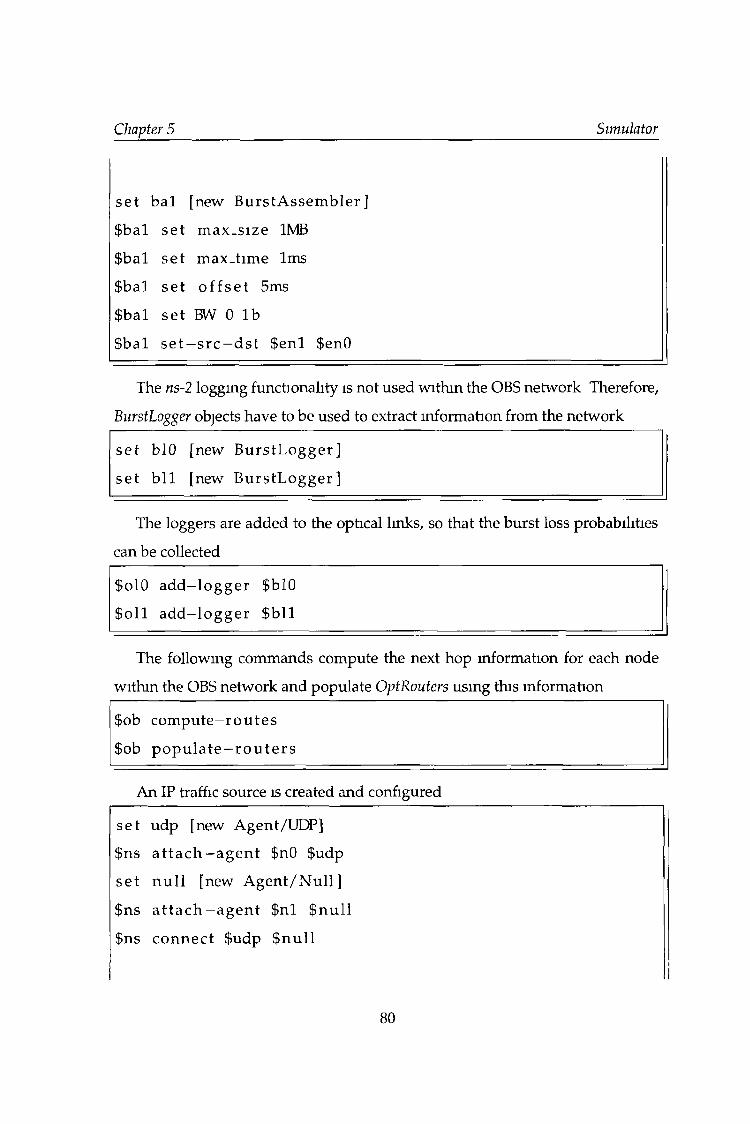
Chapter 5 Simulator
s e t b a l [new B u rs tA sse m b le r]
$ b a l s e t m a x .s iz e 1MB
$b a l s e t m ax-tim e 1ms
$b a l s e t o f f s e t 5ms
$ b a l s e t BW 0 lb
$b a l s e t - s r c - d s t $ en l $enO
The ns-2 logging functionality is not used within the OBS network Therefore,
BurstLogger objects have to be used to extract information from the network
s e t blO [new B u rs tL o g g e r]
s e t b l l [new B u rs tL o g g e r]
The loggers are added to the optical links, so that the burst loss probabilities
can be collected
o o a d d - lo g g e r $b 10
$ o ll a d d - lo g g e r $ b l l
The following commands compute the next hop information for each node
within the OBS network and populate OptRouters using this information
$ob com pute—ro u te s
$ob p o p u l a t e - r o u t e r s
An IP traffic source is created and configured
s e t udp [new Agent/UDP]
$ns a t t a c h - a g e n t $n0 $udp
s e t n u l l [new A g e n t / N u l l ]
$ns a t t a c h - a g e n t $n l $ n u l l
$ns c o n n e c t $udp $ n u l l
80
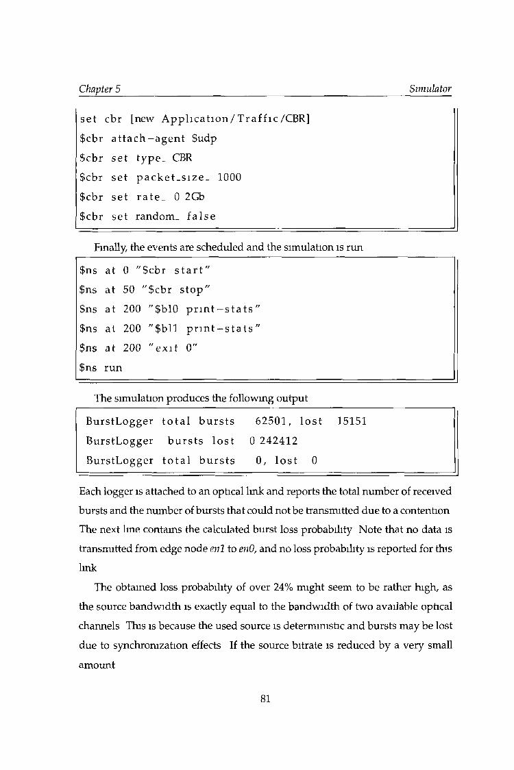
Chapter 5 Simulator
s e t cbr [new A p p l i c a t i o n / T r a f f i c / C B R ]
$cbr a t t a c h - a g e n t $udp
$cbr s e t type_ CBR
$cbr s e t p a c k e t _ s i z e _ 1000
$cbr s e t r a t e _ 0 2Gb
$cbr s e t random _ f a l s e
Finally, the events are scheduled and the simulation is run
$ns a t 0 "$cb r s t a r t "
$ns a t 50 " $ cb r s to p "
$ns a t 200 "$b l0 p r i n t - s t a t s "
$ns a t 200 " $ b l l p r i n t - s t a t s "
$ns a t 200 " e x i t 0"
$ns run
The simulation produces the following output
B urs tL ogger t o t a l b u r s t s 62501, l o s t 15151
B urs tL ogger b u r s t s l o s t 0 242412
B urs tL ogger t o t a l b u r s t s 0, l o s t 0
Each logger is attached to an optical link and reports the total number of received
bursts and the number of bursts that could not be transmitted due to a contention
The next lme contains the calculated burst loss probability Note that no data is
transmitted from edge node enl to enO, and no loss probability is reported for this
link
The obtained loss probability of over 24% might seem to be rather high, as
the source bandwidth is exactly equal to the bandwidth of two available optical
channels This is because the used source is deterministic and bursts may be lost
due to synchronization effects If the source bitrate is reduced by a very small
amount
81
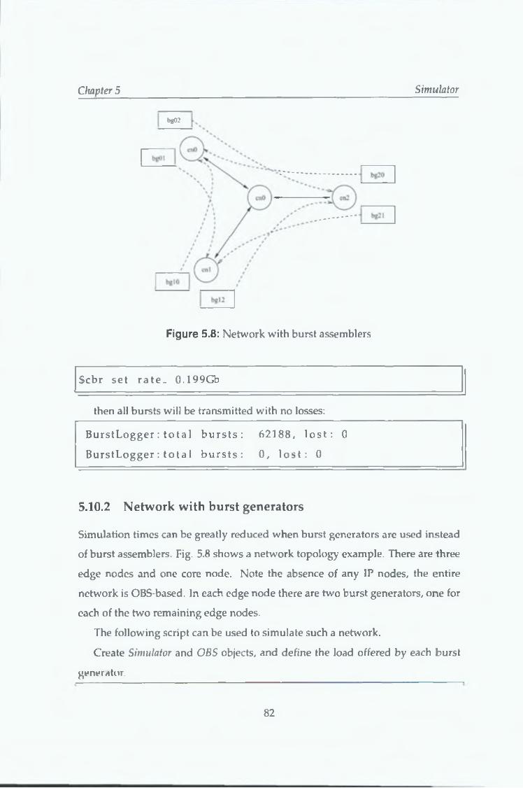
Chapter 5 Simulator
bg02
Figure 5.8: Network with burst assemblers
$cbr se t r a t e . 0.199Gb
then all bursts will be transmitted with no losses:
B u r s tL o g g e r : t o t a 1 b u r s t s : 62188, l o s t : 0
B u r s tL o g g e r : t o t a 1 b u r s t s : 0 , l o s t : 0
5.10.2 N etw ork w ith b u rst generators
Simulation times can be greatly reduced when burst generators arc used instead
of burst assemblers. Fig. 5.8 shows a network topology example. There are three
edge nodes and one core node. Note the absence of any IP nodes, the entire
network is OBS-based. In each edge node there are two burst generators, one for
each of the two remaining edge nodes.
The following script can be used to simulate such a network.
Create Simulator and OBS objects, and define the load offered by each burst
generator.
82
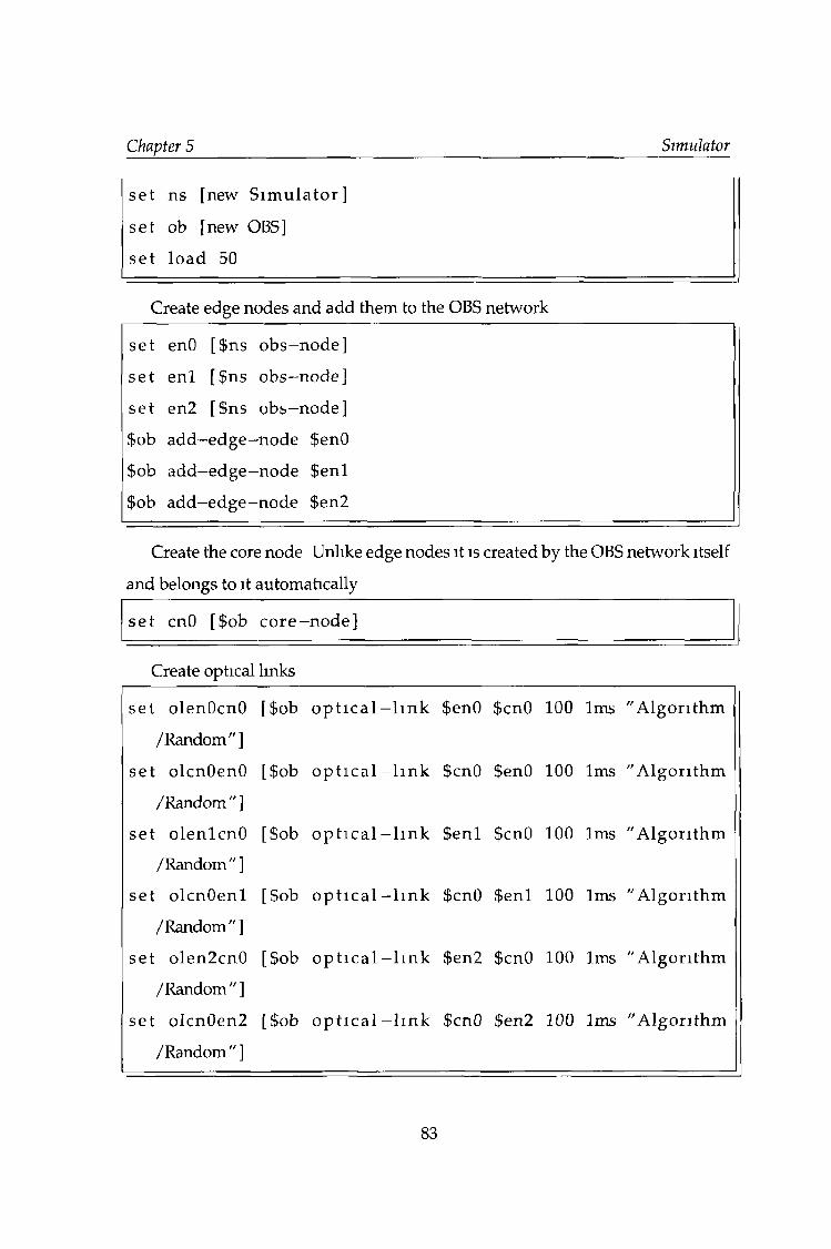
Chapter 5 Simulator
s e t ns [new S im u la to r ]
s e t ob [new OBS]
s e t load 50
Create edge nodes and add them to the OBS network
s e t enO [$ns o b s-n o d e ]
s e t en l [$ns obs—node]
se t en2 [$ns o b s-n o d e ]
$ob add--ed g e-n o d e $en0
$ob add--ed g e-n o d e $en l
$ob add--ed ge-node $en2
Create the core node Unlike edge nodes it is created by the OBS network itself
and belongs to it automatically
s e t cnO [$ob c o r e —node]
Create optical Imks
s e t olenOcnO
/Random "]
[$ob o p t i c a l - l i n k $en0 $cn0 100 1ms "A lg o r i th m
se t olcnOenO
/Random "]
[$ob o p t i c a l - l i n k $cn0 $en0 100 1ms "A lg o r i th m
se t o lenlcnO
/Random"]
[$ob o p t i c a l - l i n k $enl $cn0 100 1ms "A lg o r i th m
s e t o lcnOenl
/Random "]
[$ob o p t i c a l - l i n k $cn0 $ en l 100 1ms "A lg o r i th m
se t o len2cn0
/Random "]
[$ob o p t i c a l - l i n k $en2 $cn0 100 1ms "A lg o r i th m
s e t o lcn0en2
/Random "]
[$ob o p t i c a l —l i n k $cnO $en2 100 1ms "A lgor i thm
83
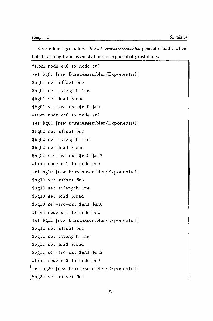
Chapter 5 Simulator
Create burst generators BurstAssembler/Exponential generates traffic where
both burst length and assembly time are exponentially distributed
#from node enO to node en l
s e t bgOl [new B u r s t A s s e m b l e r / E x p o n e n t i a l ]
$bg01 s e t o f f s e t Sms
$bg01 s e t a v l e n g th 1ms
$bg01 s e t load $ load
$bg01 s e t - s r c - d s t $enO $enl
#from node enO to node en2
s e t bg02 [new B u r s t A s s e m b l e r / E x p o n e n t i a l ]
$bg02 s e t o f f s e t 5ms
$bg02 s e t a v l e n g t h 1ms
$bg02 s e t load $ load
$bg02 s e t —s r c —d s t $enO $en2
#from node en l to node enO
s e t bglO [new B u r s t A s s e m b l e r / E x p o n e n t i a l ]
$bglO s e t o f f s e t Sms
$bglO se t a v l e n g t h 1ms
$bglO s e t load $ load
$bglO s e t —s r c —d s t $en l $enO
#from node en l to node en2
s e t b g l2 [new B u r s tA s s e m b l e r / E x p o n e n t i a l ]
$bgl2 s e t o f f s e t Sms
$bgl2 s e t a v l e n g t h 1ms
$bgl2 s e t load $ load
$bgl2 s e t - s r c - d s t $enl $en2
#from node en2 to node enO
s e t bg20 [new B u r s t A s s e m b l e r / E x p o n e n t i a l ]
$bg20 s e t o f f s e t 5ms
84
Chapter 5 Simulator
$bg20 s e t a v l e n g t h 1ms
$bg20 s e t lo ad $ load
$bg20 s e t - s r c - d s t $en2 $enO
#from node en2 to node e n l
s e t bg21 [new Burs t A s s e m b l e r / E x p o n e n t i a l ]
$bg21 s e t o f f s e t Sms
$bg21 s e t a v l e n g th 1ms
$bg21 s e t load $ load
$bg21 s e t - s r c - d s t $en2 $en l
There are six burst generators, and starting/stopping each of them separately
would be rather inconvenient Therefore, a Generatoi s helper object is used
s e t g e n e r a t o r s [new G e n e r a t o r s ]
$ g e n e r a t o r s a d d - g e n e r a t o r $bg01
$ g e n e r a t o r s a d d - g e n e r a t o r $bg01
$ g e n e r a t o r s add—g e n e r a t o r $bglO
$ g e n e r a t o r s a d d - g e n e r a t o r $bgl2
$ g e n e r a t o r s a d d - g e n e r a t o r $bg20
$ g e n e r a t o r s a d d - g e n e r a t o r $bg21
In this simulation, only the total traffic loss will be investigated In order to do
so, only two burst loggers are necessary one attached to all burst generators and
one attached to all nodes A BurstLogger/Traffic object will, among others, report
the total traffic transmitted by a generator or received by a node
s e t b l_ o u t [new B u r s t L o g g e r / T r a f f i c ]
s e t b l _ m [new B u r s t L o g g e r / T r a f f i c ]
#add l o g g e r to g e n e r a t o r s
$bg01 a d d - l o g g e r $ b l_ o u t
$bg02 a d d - l o g g e r $ b l_ o u t
$bglO a d d - l o g g e r $ b l_ o u t
85
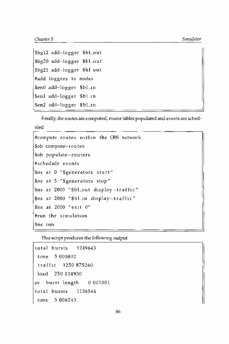
Chapter 5 Simulator
$bgl2 a d d - l o g g e r $ b l_ o u t
$bg20 a d d - l o g g e r $ b l_ o u t
$bg21 a d d - l o g g e r $ b l_ o u t
#add lo g g e r s to nodes
$enO a d d - l o g g e r $ b l_ in
$en l a d d - l o g g e r $ b l_ in
$en2 a d d - l o g g e r $ b l_ in
Finally, the routes are computed, router tables populated and events are sched
uled
#com pute r o u t e s w i t h i n the OBS ne tw ork
$ob compute—r o u t e s
$ob p o p u l a t e - r o u t e r s
# s c h e d u le e v e n ts
$ns a t 0 " $ g e n e r a t o r s s t a r t "
$ns a t 5 " $ g e n e r a t o r s s to p "
$ns a t 2000 " $ b l_ o u t d i s p l a y - t r a f f i c "
$ns at 2000 " $ b l _ i n d i s p l a y — t r a f f i c "
$ns at 2000 " e x i t 0"
#run the s i m u l a t i o n
$ns run
This script produces the following output
t o t a l b u r s t s 1249643
t ime 5 000802
t r a f f i c 1250 875260
lo ad 250 134930
av b u r s t l e n g t h 0 001001
t o t a l b u r s t s 1136544
t ime 5 006243
86
Chapter 5 Simulator
t r a f f i c 1137 429390
load 227 202172
av b u r s t l e n g t h 0 001001
This allows us to calculate the total loss in terms of both burst loss probability
(9 05%) and traffic loss (9 3%) The difference between those probabilities is a
result of a burst selecting effect, described in Chapter 3 2
5.11 Sum m ary
In this chapter, the OBS extension to the ns-2 simulator has been introduced The
building blocks of the OBS simulator have been described m detail, along with
their usage and configuration options Then, several helper objects were dis
cussed Finally, a simple simulation scenario was used to validate the simula
tor output, and two example simulation scripts were presented and described in
detail
87
Chapter 6
Results and discussion of
cost-based scheduling
The performance of the cost-based scheduling algorithm described in Chapter 4
was tested in a series of simulations Several different network topologies and
traffic types were considered In the following section the simulation procedure
is first introduced, then the performance of the cost-based algorithm and its de
pendence on several parameters is tested m a simple, single-node scenario Then,
the results for three more complex network topologies are presented
6.1 Introduction
The cost-based scheduling algorithm used m all simulations m this chapter con
siders two types of resources outgoing channels and FDL channels In other
words, when a reservation is to be made, a lowest-priced outgomg channel is
found first Then, a lowest priced channel is found agam, for a burst delayed m
a FDL, and the cost of using a FDL is added The cost of using a FDL channel is
either constant (constant strategy), or it is a function of the number of occupied
FDL channels (linear strategy) Finally, the lower of those two values is chosen
Obviously, the initial price of using a FDL channel is an important parameter
and its choice will affect the network performance Fig 6 1 shows how the burst
loss probability is expected to change when the FDL price is adjusted At first
(poin t"A"), when the price is low, the algorithm will tend to use most of the FDL
channels to improve the alignment of bursts within a channel However, when
88
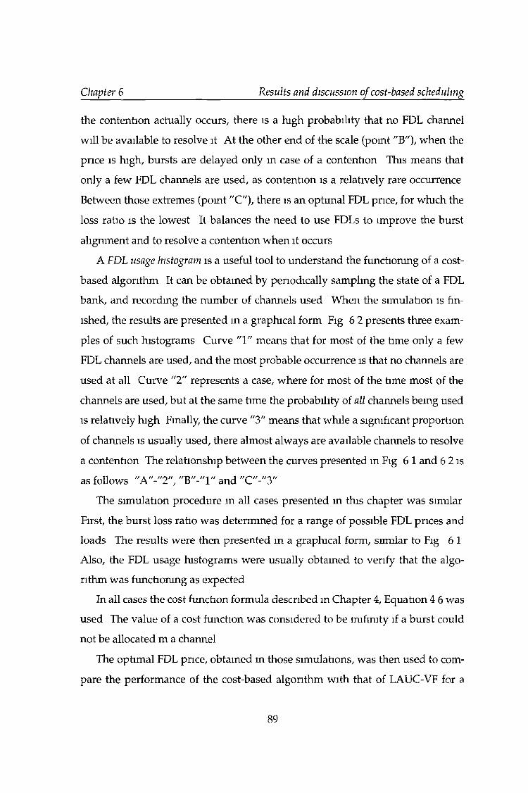
Chapter 6 Results and discussion of cost-based scheduling
the contention actually occurs, there is a high probability that no FDL channel
will be available to resolve it At the other end of the scale (point "B"), when the
price is high, bursts are delayed only in case of a contention This means that
only a few FDL channels are used, as contention is a relatively rare occurrence
Between those extremes (point "C"), there is an optimal FDL price, for which the
loss ratio is the lowest It balances the need to use FDLs to improve the burst
alignment and to resolve a contention when it occurs
A FDL usage histogram is a useful tool to understand the functioning of a cost-
based algorithm It can be obtained by periodically sampling the state of a FDL
bank, and recording the number of channels used When the simulation is fin
ished, the results are presented m a graphical form Fig 6 2 presents three exam
ples of such histograms Curve "1" means that for most of the time only a few
FDL channels are used, and the most probable occurrence is that no channels are
used at all Curve "2" represents a case, where for most of the time most of the
channels are used, but at the same time the probability of all channels being used
is relatively high Finally, the curve "3" means that while a significant proportion
of channels is usually used, there almost always are available channels to resolve
a contention The relationship between the curves presented in Fig 6 1 and 6 2 is
as follows "A"-"2", "B"-"l" and "C"-"3"
The simulation procedure in all cases presented in this chapter was similar
First, the burst loss ratio was determined for a range of possible FDL prices and
loads The results were then presented m a graphical form, similar to Fig 6 1
Also, the FDL usage histograms were usually obtained to verify that the algo
rithm was functioning as expected
In all cases the cost function formula described in Chapter 4, Equation 4 6 was
used The value of a cost function was considered to be mifmity if a burst could
not be allocated m a channel
The optimal FDL price, obtained m those simulations, was then used to com
pare the performance of the cost-based algorithm with that of LAUC-VF for a
89
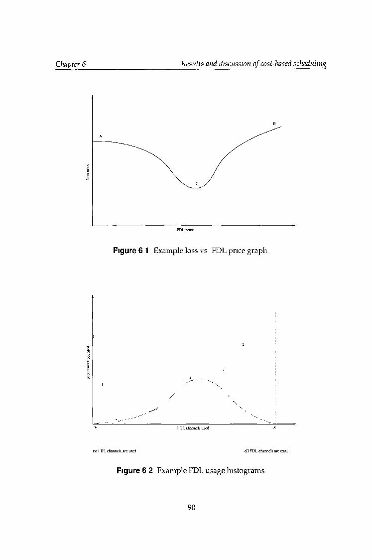
occu
renc
es
coun
ted
loss
ratio
Chapter 6 Results and discussion of cost-based scheduling
Figure 6 1 Example loss vs FDL price graph
-‘i.
l-DL channcis used
no FDL channels arc used all FDL channcis arc used
Figure 6 2 Example FDL usage histograms
90
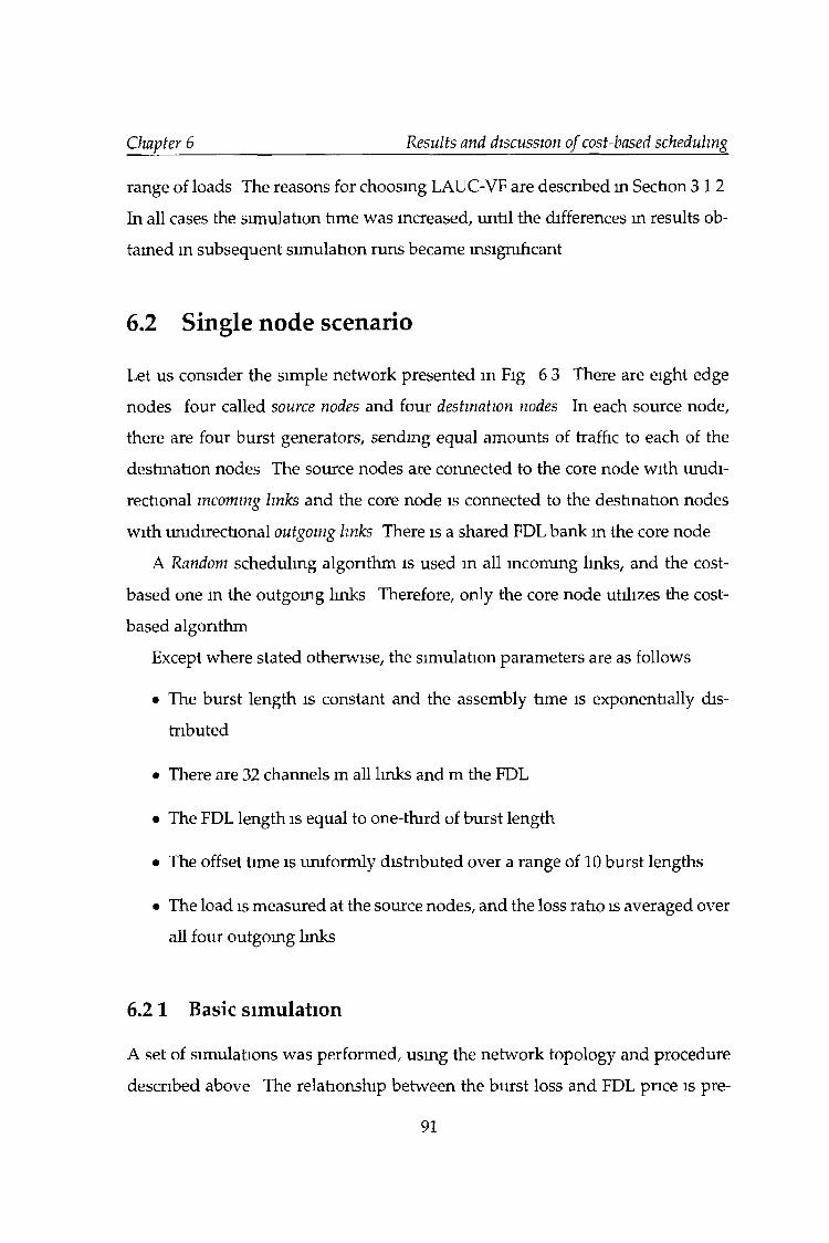
Chapter 6 Results and discussion of cost-based scheduling
range of loads The reasons for choosing LAUC-VF are described in Section 3 1 2
In all cases the simulation time was increased, until the differences in results ob
tained m subsequent simulation runs became insignificant
6.2 Single node scenario
Let us consider the simple network presented m Fig 6 3 There are eight edge
nodes four called source nodes and four destination nodes In each source node,
there are four burst generators, sending equal amounts of traffic to each of the
destination nodes The source nodes are connected to the core node with unidi
rectional incoming links and the core node is connected to the destination nodes
with unidirectional outgoing links There is a shared FDL bank in the core node
A Random scheduling algorithm is used in all incoming links, and the cost-
based one in the outgoing links Therefore, only the core node utilizes the cost-
based algorithm
Except where stated otherwise, the simulation parameters are as follows
• The burst length is constant and the assembly time is exponentially dis
tributed
• There are 32 channels m all links and m the FDL
• The FDL length is equal to one-third of burst length
• The offset time is uniformly distributed over a range of 10 burst lengths
• The load is measured at the source nodes, and the loss ratio is averaged over
all four outgomg links
6.2 1 Basic simulation
A set of simulations was performed, using the network topology and procedure
described above The relationship between the burst loss and FDL price is pre-
91
Chapter 6 Results and discussion of cost-based scheduling
Figure 6 3 Single-node network topology
sented in Fig 6 4-6 6
It is apparent that the loss ratio is relatively high when the cost of using a
FDL is zero, then it drops markedly and finally rises agam This effect can be
explained as follows when the FDL price is very low, a burst will be delayed
every time when it will result m a better alignment with other bursts However,
this will also result m most of the FDL channels being occupied for most of the
time This is not an optimal solution, because when a contention occurs there will
be no way to resolve it
At the other end of the range, when the FDL price is very high, a burst will
only be delayed when it is impossible to allocate it otherwise Unfortunately, as
no bursts will be delayed in order to improve their alignment with other bursts,
the probability of contention will be quite high Also, this approach results in a
majority of FDL channels being unused for most of the time
Consequently, between those extremes, there is a certain FDL cost for which
the traffic loss is the lowest An examination of the results presented m Fig 6 4-6 6
leads to the following conclusions
• Both strategies offer similar minimum loss ratio,
92
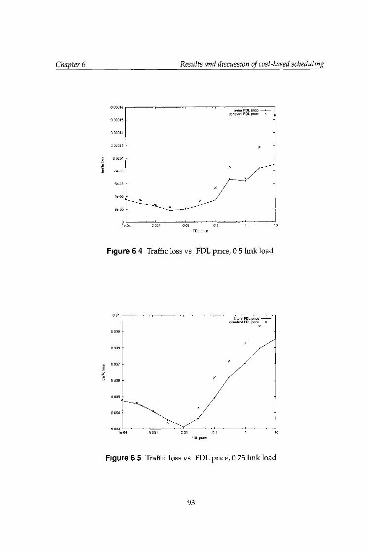
Chapter 6 Results and discussion of cost-based scheduling
Figure 6 4 Traffic loss vs FDL price, 0 5 link load
FDL price
Figure 6 5 Traffic loss vs FDL price, 0 75 link load
93
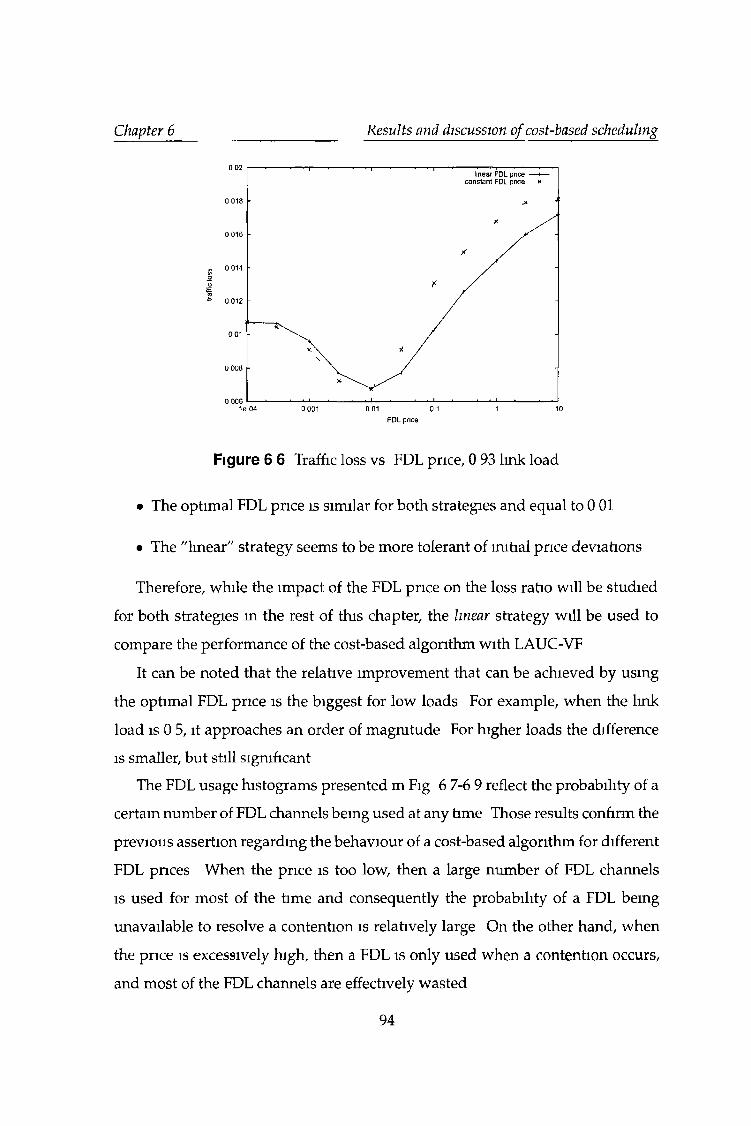
Chapter 6 Results and discussion of cost-based scheduling
FDL price
Figure 6 6 Traffic loss vs FDL price, 0 93 link load
• The optimal FDL price is similar for both strategies and equal to 0 01
• The "linear" strategy seems to be more tolerant of initial price deviations
Therefore, while the impact of the FDL price on the loss ratio will be studied
for both strategies in the rest of this chapter, the linear strategy will be used to
compare the performance of the cost-based algorithm with LAUC-VF
It can be noted that the relative improvement that can be achieved by using
the optimal FDL price is the biggest for low loads For example, when the link
load is 0 5, it approaches an order of magnitude For higher loads the difference
is smaller, but still significant
The FDL usage histograms presented m Fig 6 7-6 9 reflect the probability of a
certam number of FDL channels bemg used at any time Those results confirm the
previous assertion regarding the behaviour of a cost-based algorithm for different
FDL prices When the price is too low, then a large number of FDL channels
is used for most of the time and consequently the probability of a FDL bemg
unavailable to resolve a contention is relatively large On the other hand, when
the price is excessively high, then a FDL is only used when a contention occurs,
and most of the FDL channels are effectively wasted
94
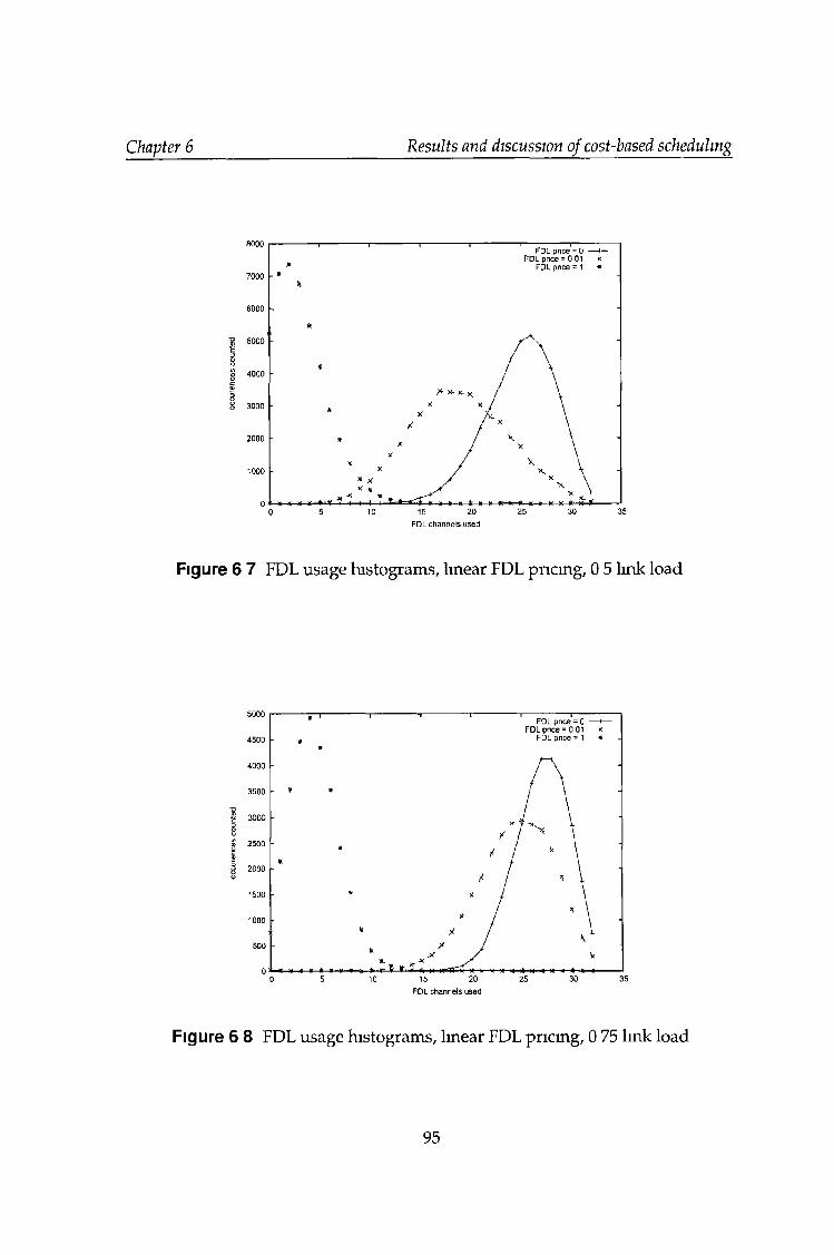
Chapter 6 Results and discussion of cost-based scheduling
FDL channels used
Figure 6 7 FDL usage histograms, linear FDL pricing, 0 5 link load
FDL channels used
Figure 6 8 FDL usage histograms, linear FDL pncmg, 0 75 link load
95
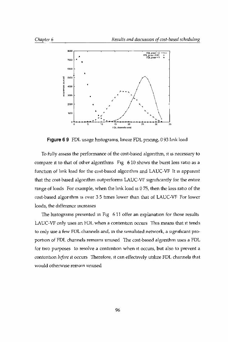
Chapter 6 Results and discussion of cost-based scheduling
FDL channels used
Figure 6 9 FDL usage histograms, linear FDL pricing, 0 93 link load
To fully assess the performance of the cost-based algorithm, it is necessary to
compare it to that of other algorithms Fig 6 10 shows the burst loss ratio as a
function of link load for the cost-based algorithm and LAUC-VF It is apparent
that the cost-based algorithm outperforms LAUC-VF significantly for the entire
range of loads For example, when the link load is 0 75, then the loss ratio of the
cost-based algorithm is over 3 5 times lower than that of LAUC-VF For lower
loads, the difference increases
The histograms presented m Fig 6 11 offer an explanation for those results
LAUC-VF only uses an FDL when a contention occurs This means that it tends
to only use a few FDL channels and, in the simulated network, a significant pro
portion of FDL channels remains unused The cost-based algorithm uses a FDL
for two purposes to resolve a contention when it occurs, but also to prevent a
contention before it occurs Therefore, it can effectively utilize FDL channels that
would otherwise remam unused
96
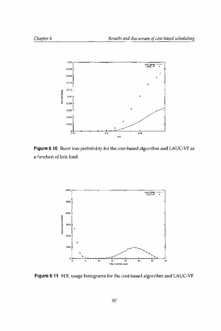
Chapter 6 Results and discussion of cost-based scheduling
load
Figure 610 Burst loss probability for the cost-based algorithm and LAUC-VF as
a function of link load
FDL channels used
Figure 6 11 FDL usage histograms for the cost-based algorithm and LAUC-VF
97
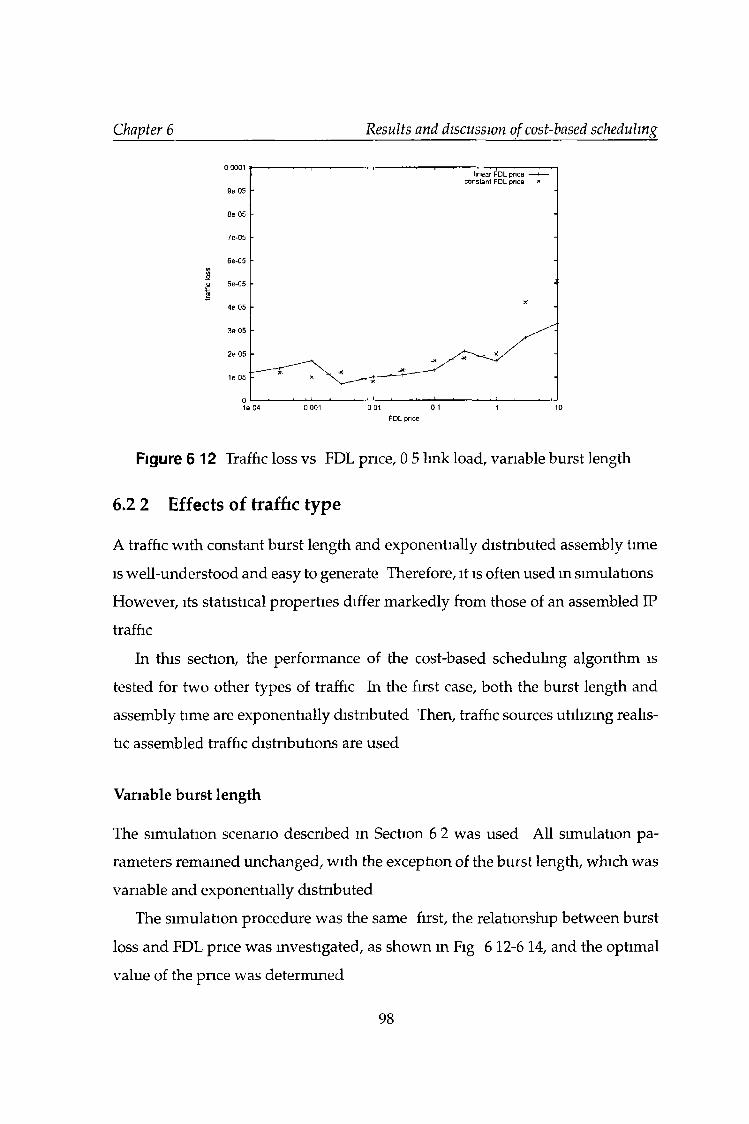
Chapter 6 Results and discussion of cost-based scheduling
FDL price
Figure 612 Traffic loss vs FDL price, 0 5 link load, variable burst length
6.2 2 Effects of traffic type
A traffic with constant burst length and exponentially distributed assembly time
is well-understood and easy to generate Therefore, it is often used m simulations
However, its statistical properties differ markedly from those of an assembled IP
traffic
In this section, the performance of the cost-based scheduling algorithm is
tested for two other types of traffic In the first case, both the burst length and
assembly time are exponentially distributed Then, traffic sources utilizing realis
tic assembled traffic distributions are used
Variable burst length
The simulation scenario described in Section 6 2 was used All simulation pa
rameters remained unchanged, with the exception of the burst length, which was
variable and exponentially distributed
The simulation procedure was the same first, the relationship between burst
loss and FDL price was investigated, as shown in Fig 6 12-6 14, and the optimal
value of the price was determined
98
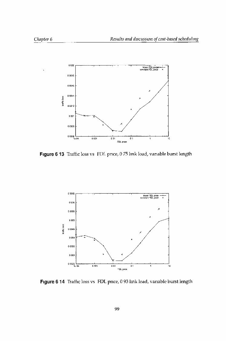
Chapter 6 Results and discussion of cost-based scheduling
FDL price
Figure 613 Traffic loss vs FDL price, 0 75 link load, variable burst length
FDL price
Figure 614 Traffic loss vs FDL price, 0 93 link load, variable burst length
99
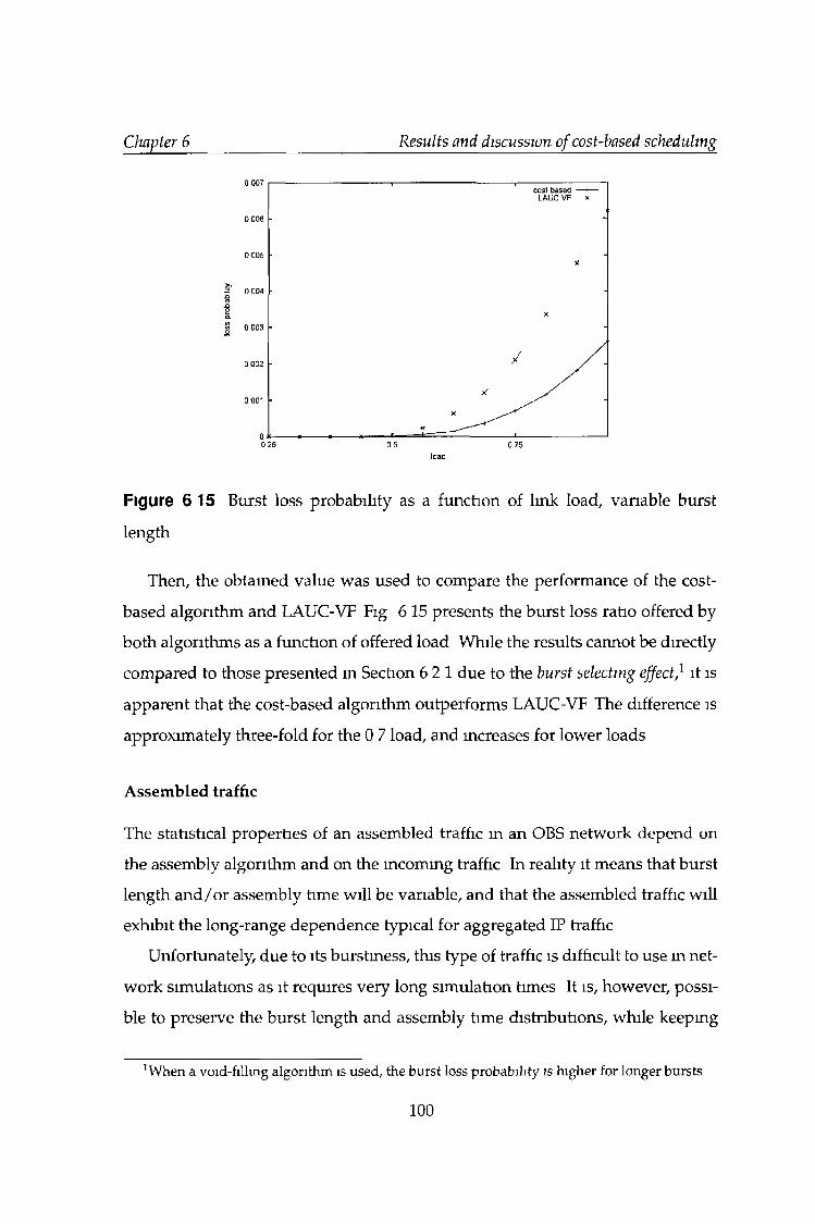
Chapter 6 Results and discussion of cost-based scheduling
load
Figure 615 Burst loss probability as a function of link load, variable burst
length
Then, the obtained value was used to compare the performance of the cost-
based algorithm and LAUC-VF Fig 6 15 presents the burst loss ratio offered by
both algorithms as a function of offered load While the results cannot be directly
compared to those presented m Section 6 21 due to the burst selecting effect} it is
apparent that the cost-based algorithm outperforms LAUC-VF The difference is
approximately three-fold for the 0 7 load, and mcreases for lower loads
A ssem bled traffic
The statistical properties of an assembled traffic m an OBS network depend on
the assembly algorithm and on the incoming traffic In reality it means that burst
length an d /o r assembly time will be variable, and that the assembled traffic will
exhibit the long-range dependence typical for aggregated IP traffic
Unfortunately, due to its burstiness, this type of traffic is difficult to use in net
work simulations as it requires very long simulation times It is, however, possi
ble to preserve the burst length and assembly time distributions, while keeping
1W hen a void-filling algorithm is used, the burst loss probability is higher for longer bursts
100
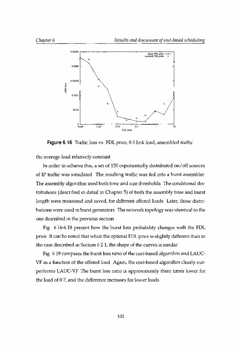
Chapter 6 Results and discussion of cost-based scheduling
FDL price
Figure 616 Traffic loss vs FDL price, 0 5 link load, assembled traffic
the average load relatively constant
In order to achieve this, a set of 150 exponentially distributed on/off sources
of IP traffic was simulated The resulting traffic was fed into a burst assembler
The assembly algorithm used both time and size thresholds The conditional dis
tributions (described m detail in Chapter 5) of both the assembly time and burst
length were measured and saved, for different offered loads Later, those distri
butions were used in burst generators The network topology was identical to the
one described in the previous section
Fig 6 16-6 18 present how the burst loss probability changes with the FDL
price It can be noted that while the optimal FDL price is slightly different than m
the case described in Section 6 21, the shape of the curves is similar
Fig 6 19 compares the burst loss ratio of the cost-based algorithm and LAUC-
VF as a function of the offered load Again, the cost-based algorithm clearly out
performs LAUC-VF The burst loss ratio is approximately three times lower for
the load of 0 7, and the difference mcreases for lower loads
101
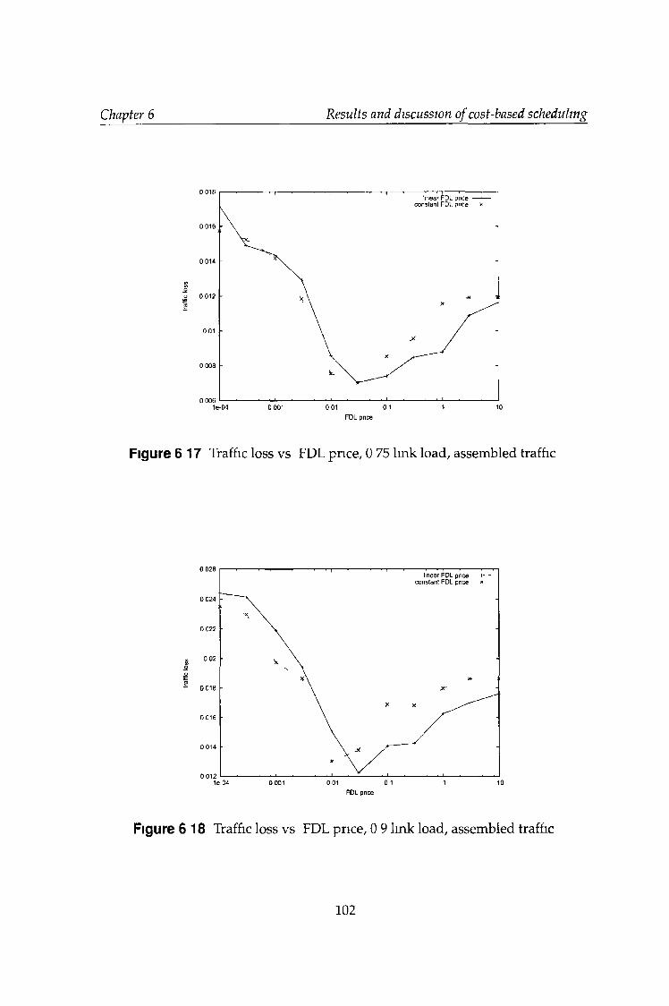
Chapter 6 Results and discussion of cost-based scheduling
FDL price
Figure 6 17 Traffic loss vs FDL price, 0 75 link load, assembled traffic
FDL price
Figure 6 18 Traffic loss vs FDL price, 0 9 link load, assembled traffic
102
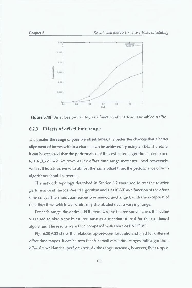
Chapter 6 Results and discussion o f cost-based scheduling
bad
Figure 6.19: Burst loss probability as a function of link load, assembled traffic.
6.2.3 Effects of offset tim e range
The greater the range of possible offset times, the better the chances that a better
alignment of bursts within a channel can be achieved by using a FDL. Therefore,
it can be expected that the performance of the cost-based algorithm as compared
to LAUC-VF will improve as the offset time range increases. And conversely,
when all bursts arrive with almost the same offset time, the performance of both
algorithms should converge.
The network topology described in Section 6.2 was used to test the relative
performance of the cost-based algorithm and LAUC-VF as a function of the offset
time range. The simulation scenario remained unchanged, with the exception of
the offset time, which was uniformly distributed over a varying range.
For each range, the optimal FDL price was first determined. Then, this value
was used to obtain the burst loss ratio as a function of load for the cost-based
algorithm. The results were then compared with those of LAUC-VF.
Fig. 6.20-6.23 show the relationship between loss ratio and load for different
offset time ranges. It can be seen that for small offset time ranges both algorithms
offer almost identical performance. As the range increases, however, their respec-
103
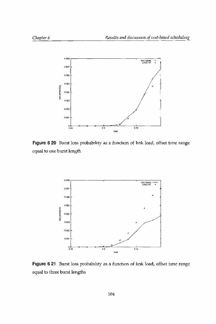
Chapter 6 Results and discussion of cost-based scheduling
load
Figure 6 20 Burst loss probability as a function of link load, offset time range
equal to one burst length
load
Figure 6 21 Burst loss probability as a function of link load, offset tune range
equal to three burst lengths
104
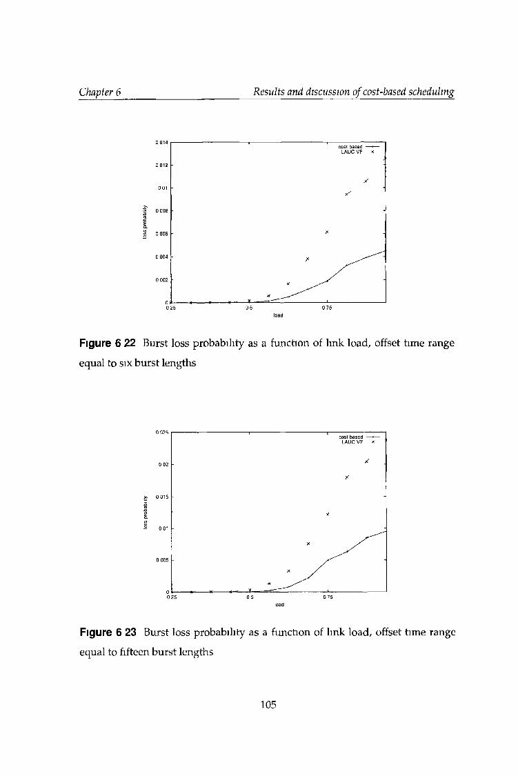
Chapter 6 Results and discussion of cost-based scheduling
load
Figure 6 22 Burst loss probability as a function of link load, offset time range
equal to six burst lengths
load
Figure 6 23 Burst loss probability as a function of link load, offset time range
equal to fifteen burst lengths
105
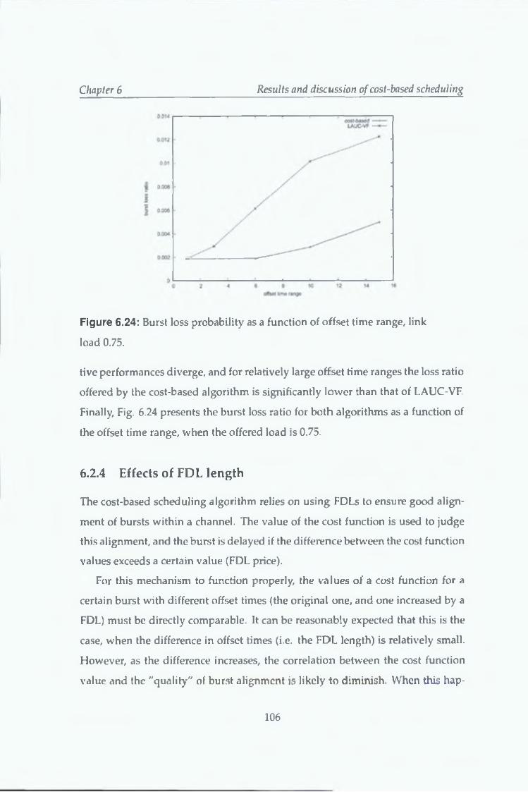
Chapter 6 Results and discussion o f cost-based scheduling
Figure 6.24: Burst loss probability as a function of offset time range, link
load 0.75.
tive performances diverge, and for relatively large offset time ranges the loss ratio
offered by the cost-based algorithm is significantly lower than that of LAUC-VF.
Finally, Fig. 6.24 presents the burst loss ratio for both algorithms as a function of
the offset time range, when the offered load is 0.75.
6.2.4 Effects of FDL length
The cost-based scheduling algorithm relies on using FDLs to ensure good align
ment of bursts within a channel. The value of the cost function is used to judge
this alignment, and the burst is delayed if the difference between the cost function
values exceeds a certain value (FDL price).
For this mechanism to function properly, the values of a cost function for a
certain burst with different offset times (the original one, and one increased by a
FDL) must be directly comparable. It can be reasonably expected that this is the
case, when the difference in offset times (i.e. the FDL length) is relatively small.
However, as the difference increases, the correlation between the cost function
value and the "quality" of burst alignment is likely to diminish. When this hap-
10 6
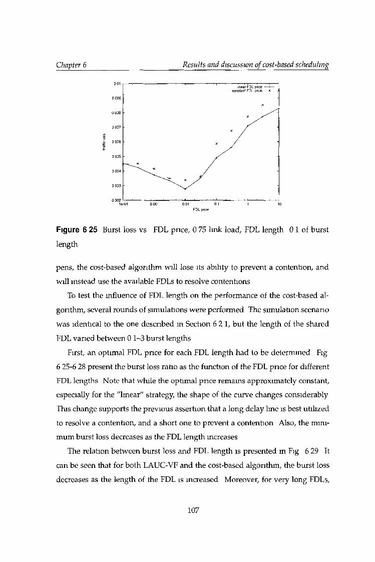
Chapter 6 Results and discussion of cost-based scheduling
FDL price
Figure 6 25 Burst loss vs FDL price, 0 75 link load, FDL length 0 1 of burst
length
pens, the cost-based algorithm will lose its ability to prevent a contention, and
will instead use the available FDLs to resolve contentions
To test the influence of FDL length on the performance of the cost-based al
gorithm, several rounds of simulations were performed The simulation scenario
was identical to the one described in Section 6 21, but the length of the shared
FDL varied between 0 1-3 burst lengths
First, an optimal FDL price for each FDL length had to be determined Fig
6 25-6 28 present the burst loss ratio as the function of the FDL price for different
FDL lengths Note that while the optimal price remains approximately constant,
especially for the "linear" strategy, the shape of the curve changes considerably
This change supports the previous assertion that a long delay line is best utilized
to resolve a contention, and a short one to prevent a contention Also, the mini
mum burst loss decreases as the FDL length increases
The relation between burst loss and FDL length is presented m Fig 6 29 It
can be seen that for both LAUC-VF and the cost-based algorithm, the burst loss
decreases as the length of the FDL is increased Moreover, for very long FDLs,
107
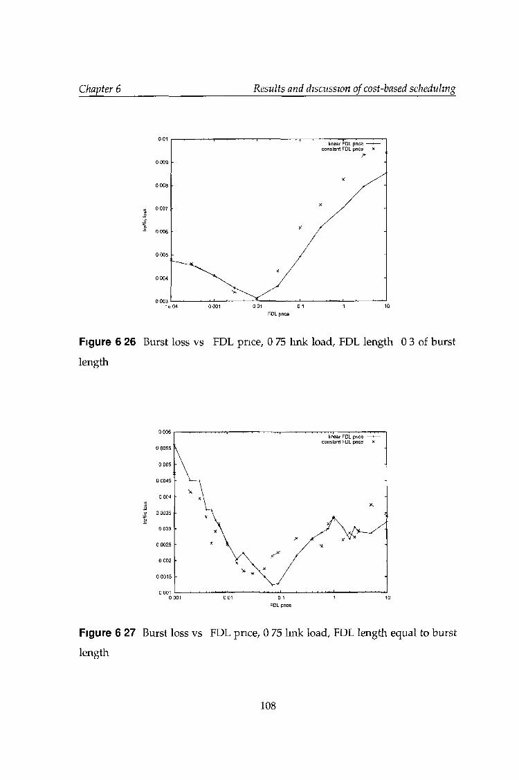
Chapter 6 Results and discussion of cost-based scheduling
FDL price
Figure 6 26 Burst loss vs FDL price, 0 75 link load, FDL length 0 3 of burst
length
FDL price
Figure 6 27 Burst loss vs FDL price, 0 75 link load, FDL length equal to burst
length
108
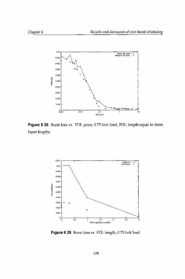
Chapter 6 Results and discussion of cost-based scheduling
FDL price
Figure 6 28 Burst loss vs FDL price, 0 75 link load, FDL length equal to three
burst lengths
Figure 6 29 Burst loss vs FDL length, 0 75 link load
109
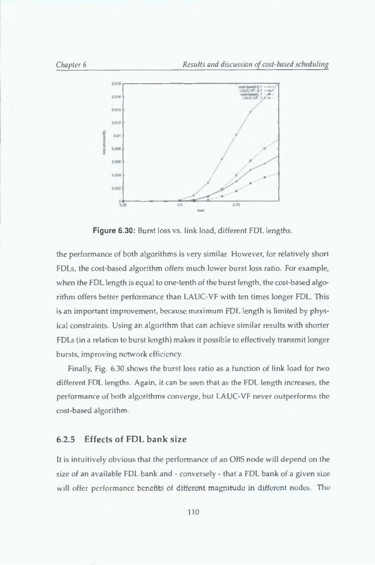
Chapiter 6 Results and discussion of cost-based scheduling
toad
Figure 6.30: Burst loss vs. link load, different FDL lengths.
the performance of both algorithms is very similar. However, for relatively short
FDLs, the cost-based algorithm offers much lower burst loss ratio. For example,
when the FDL length is equal to one-tenth of the burst length, the cost-based algo
rithm offers better performance than LAUC-VF with ten times longer FDL. This
is an important improvement, because maximum FDL length is limited by phys
ical constraints. Using an algorithm that can achieve similar results with shorter
FDLs (in a relation to burst length) makes it possible to effectively transmit longer
bursts, improving network efficiency.
Finally, Fig. 6.30 shows the burst loss ratio as a function of link load for two
different FDL lengths. Again, it can be seen that as the FDL length increases, the
performance of both algorithms converge, but LAUC-VF never outperforms the
cost-based algorithm.
6.2.5 Effects of FDL b ank size
It is intuitively obvious that the performance of an OBS node will depend on the
size of an available FDL bank and - conversely - that a FDL bank of a given size
will offer performance benefits of different magnitude in different nodes. The
110
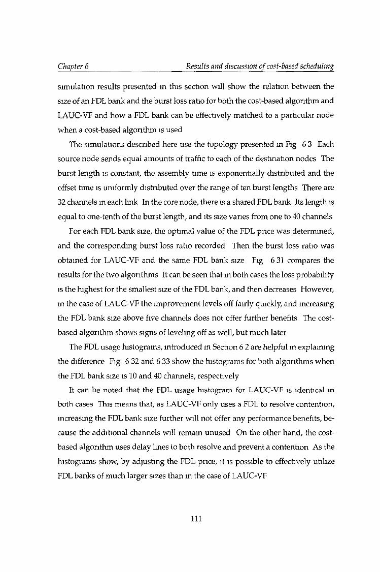
Chapter 6 Results and discussion of cost-based scheduling
simulation results presented in this section will show the relation between the
size of an FDL bank and the burst loss ratio for both the cost-based algorithm and
LAUC-VF and how a FDL bank can be effectively matched to a particular node
when a cost-based algorithm is used
The simulations described here use the topology presented in Fig 6 3 Each
source node sends equal amounts of traffic to each of the destination nodes The
burst length is constant, the assembly time is exponentially distributed and the
offset time is uniformly distributed over the range of ten burst lengths There are
32 channels m each lmk In the core node, there is a shared FDL bank Its length is
equal to one-tenth of the burst length, and its size varies from one to 40 channels
For each FDL bank size, the optimal value of the FDL price was determined,
and the corresponding burst loss ratio recorded Then the burst loss ratio was
obtained for LAUC-VF and the same FDL bank size Fig 6 31 compares the
results for the two algorithms It can be seen that in both cases the loss probability
is the highest for the smallest size of the FDL bank, and then decreases However,
in the case of LAUC-VF the improvement levels off fairly quickly, and increasing
the FDL bank size above five channels does not offer further benefits The cost-
based algorithm shows signs of leveling off as well, but much later
The FDL usage histograms, introduced m Section 6 2 are helpful in explaining
the difference Fig 6 32 and 6 33 show the histograms for both algorithms when
the FDL bank size is 10 and 40 channels, respectively
It can be noted that the FDL usage histogram for LAUC-VF is identical in
both cases This means that, as LAUC-VF only uses a FDL to resolve contention,
increasing the FDL bank size further will not offer any performance benefits, be
cause the additional channels will remam unused On the other hand, the cost-
based algorithm uses delay lmes to both resolve and prevent a contention As the
histograms show, by adjusting the FDL price, it is possible to effectively utilize
FDL banks of much larger sizes than m the case of LAUC-VF
111
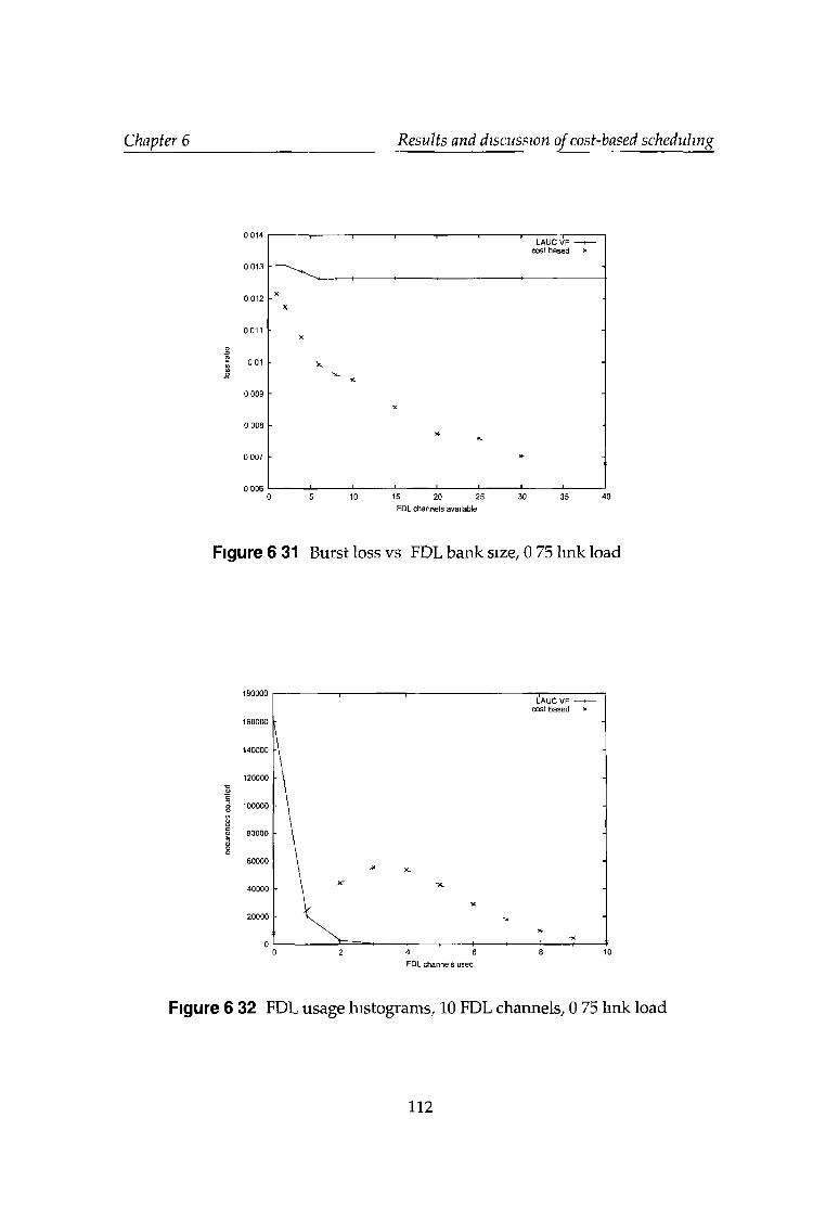
Chapter 6 Results and discussion of cost-based scheduling
FDL channels available
Figure 6 31 Burst loss vs FDL bank size, 0 75 link load
FDL channels used
Figure 6 32 FDL usage histograms, 10 FDL channels, 0 75 link load
112
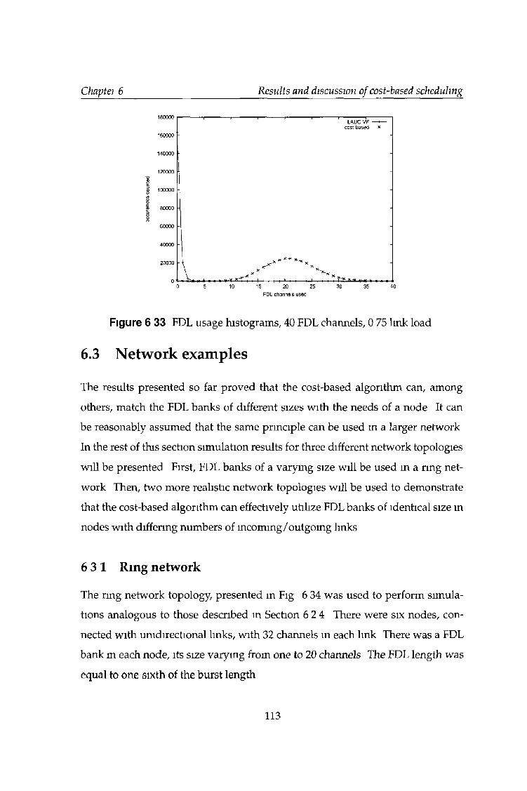
Chaptei 6 Results and discussion of cost-based scheduling
180000
160000
140000
120000T 3 £Cg 100000(0 ID O
® 80000 D 8 o
60000
40000
20000
00 5 10 15 20 25 30 35 40
FDL channels used
Figure 6 33 FDL usage histograms, 40 FDL channels, 0 75 link load
6.3 Network examples
The results presented so far proved that the cost-based algorithm can, among
others, match the FDL banks of different sizes with the needs of a node It can
be reasonably assumed that the same principle can be used in a larger network
In the rest of this section simulation results for three different network topologies
will be presented First, FDL banks of a varying size will be used m a ring net
work Then, two more realistic network topologies will be used to demonstrate
that the cost-based algorithm can effectively utilize FDL banks of identical size in
nodes with differing numbers of incoming/outgomg links
6 3 1 R ing netw ork
The ring network topology, presented in Fig 6 34 was used to perform simula
tions analogous to those described m Section 6 2 4 There were six nodes, con
nected with unidirectional links, with 32 channels in each link There was a FDL
bank m each node, its size varying from one to 20 channels The FDL length was
equal to one-sixth of the burst length
113
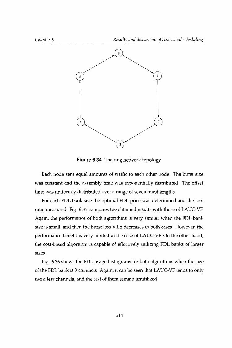
Chapter 6 Results and discussion of cost-based scheduling
Figure 6 34 The ring network topology
Each node sent equal amounts of traffic to each other node The burst size
was constant and the assembly time was exponentially distributed The offset
time was uniformly distributed over a range of seven burst lengths
For each FDL bank size the optimal FDL price was determmed and the loss
ratio measured Fig 6 35 compares the obtamed results with those of LAUC-VF
Again, the performance of both algorithms is very similar when the FDL bank
size is small, and then the burst loss ratio decreases in both cases However, the
performance benefit is very limited in the case of LAUC-VF On the other hand,
the cost-based algorithm is capable of effectively utilizing FDL banks of larger
sizes
Fig 6 36 shows the FDL usage histograms for both algorithms when the size
of the FDL bank is 9 channels Again, it can be seen that LAUC-VF tends to only
use a few channels, and the rest of them remam unutilized
114
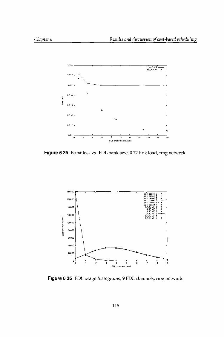
Chapter 6 Results and discussion of cost-based scheduling
FDL channels available
Figure 6 35 Burst loss vs FDL bank size, 0 72 link load, ring network
4 5FDL channels used
Figure 6 36 FDL usage histograms, 9 FDL channels, ring network
115
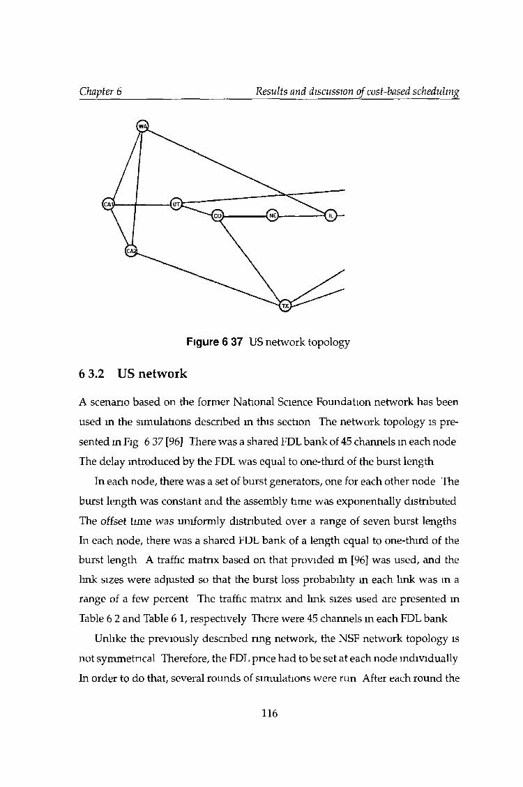
Chapter 6 Results and discussion of cost-based scheduling
Figure 6 37 US network topology
6 3.2 US netw ork
A scenario based on the former National Science Foundation network has been
used in the simulations described in this section The network topology is pre
sented m Fig 6 37 [96] There was a shared FDL bank of 45 channels in each node
The delay introduced by the FDL was equal to one-third of the burst length
In each node, there was a set of burst generators, one for each other node The
burst length was constant and the assembly time was exponentially distributed
The offset fame was uniformly distributed over a range of seven burst lengths
In each node, there was a shared FDL bank of a length equal to one-third of the
burst length A traffic matrix based on that provided m [96] was used, and the
link sizes were adjusted so that the burst loss probability in each link was in a
range of a few percent The traffic matrix and link sizes used are presented m
Table 6 2 and Table 6 1, respectively There were 45 channels m each FDL bank
Unlike the previously described ring network, the NSF network topology is
not symmetrical Therefore, the FDL price had to be set at each node individually
In order to do that, several rounds of simulations were run After each round the
116
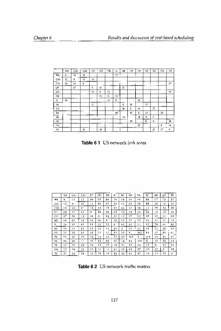
Chapter 6 Results and discussion of cost-based scheduling
WA CAI CA2 UT CO NE IL MI NY PA NJ DC CA TX
WA X 12 19 27
CAI 12 X 13 16
CA2 20 14 X 27
UT 17 X 16 20
CO 16 X 13 15
NE 11 X 13
IL 26 11 X 40
MI 21 X 33 12
NY 30 X 45 27
PA 40 47 X 17 33
NJ 13 18 X 7
DC 29 8 X 28
GA 27 X 19
TX 31 20 27 17 X
Table 6 1 US network link sizes
WA CAI CA2 UT c o NE IL MI NY PA NJ DC GA TX
WA X 12 1 3 0 8 0 7 0 6 26 1 4 21 16 0 6 1 7 13 21
CAI 1 2 X 2 6 1 1 0 9 0 7 3 2 1 7 2 5 2 0 0 8 2 0 1 6 2 6
CA2 13 2 6 X 1 5 1 3 10 4 7 2 4 3 7 2 8 1 1 2 9 2 3 3 8
UT 0 8 11 15 X 0 8 0 6 2 3 1 3 1 8 1 4 0 6 15 12 2 0
c o 0 7 0 9 1 3 0 8 X 0 6 22 12 1 7 13 0 5 15 11 2 0
NE 0 6 0 7 1 0 0 6 0 6 X 2 2 13 1 7 13 0 5 1 7 ] 1 1 9
IL 2 6 3 2 4 7 2 3 22 2 2 X 6 3 91 7 2 2 7 7 4 61 8 6
MI 14 17 2 4 1 3 1 2 1 3 6 3 X 5 5 4 3 1 6 51 3 5 4 2
NY 21 2 5 3 7 18 17 17 91 55 X 162 8 4 5 7 8 4 61
PA 1 6 2 0 2 8 14 1 3 13 7 2 4 3 162 X 11 8 4 4 9 7 4 7
NJ 0 6 0 8 1 1 0 6 0 5 0 5 2 7 1 6 8 4 11 8 X 17 1 3 0 1 8
DC 17 2 0 2 9 15 1 5 1 7 7 4 51 5 7 4 4 1 7 X 3 7 51
GA 1 3 16 2 3 1 2 11 1 1 61 3 5 8 4 9 7 3 0 3 7 X 3 9
TX 21 2 6 3 8 2 0 20 19 8 6 4 2 61 4 7 1 8 51 3 9 X
Table 6 2 US network traffic matrix
117
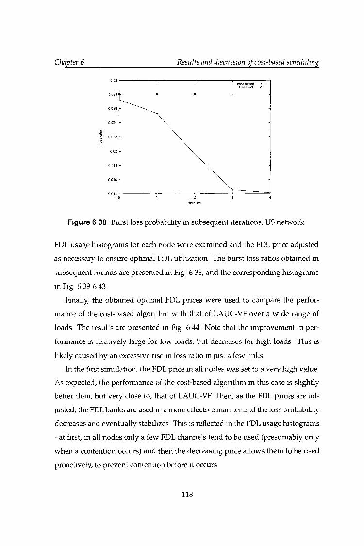
Chapter 6 Results and discussion of cost-based scheduling
Figure 6 38 Burst loss probability in subsequent iterations, US network
FDL usage histograms for each node were examined and the FDL price adjusted
as necessary to ensure optimal FDL utilization The burst loss ratios obtained m
subsequent rounds are presented in Fig 6 38, and the corresponding histograms
in Fig 6 39-6 43
Finally, the obtamed optimal FDL prices were used to compare the perfor
mance of the cost-based algorithm with that of LAUC-VF over a wide range of
loads The results are presented m Fig 6 44 Note that the improvement in per
formance is relatively large for low loads, but decreases for high loads This is
likely caused by an excessive rise in loss ratio m just a few links
In the first simulation, the FDL price m all nodes was set to a very high value
As expected, the performance of the cost-based algorithm m this case is slightly
better than, but very close to, that of LAUC-VF Then, as the FDL prices are ad
justed, the FDL banks are used in a more effective manner and the loss probability
decreases and eventually stabilizes This is reflected m the FDL usage histograms
- at first, m all nodes only a few FDL channels tend to be used (presumably only
when a contention occurs) and then the decreasing price allows them to be used
proactively, to prevent contention before it occurs
118
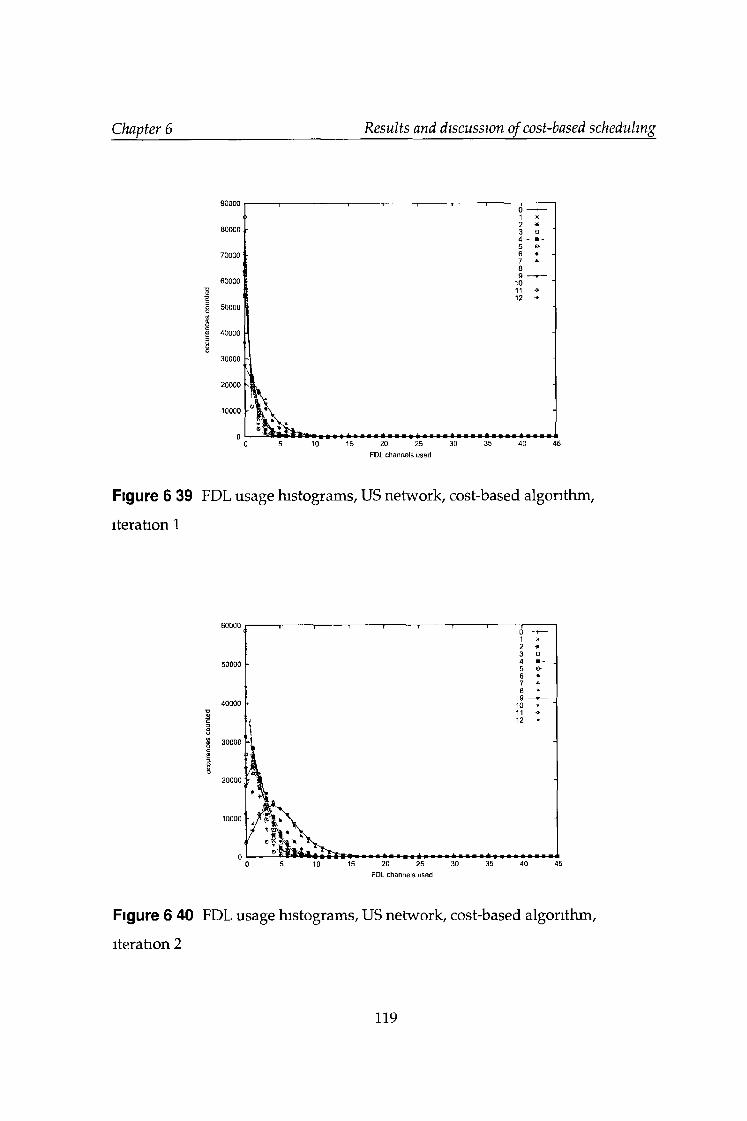
Chapter 6 Results and discussion of cost-based scheduling
Figure 6 39 FDL usage histograms, US network, cost-based algorithm,
iteration 1
FDL channels used
Figure 6 40 FDL usage histograms, US network, cost-based algorithm,
iteration 2
119
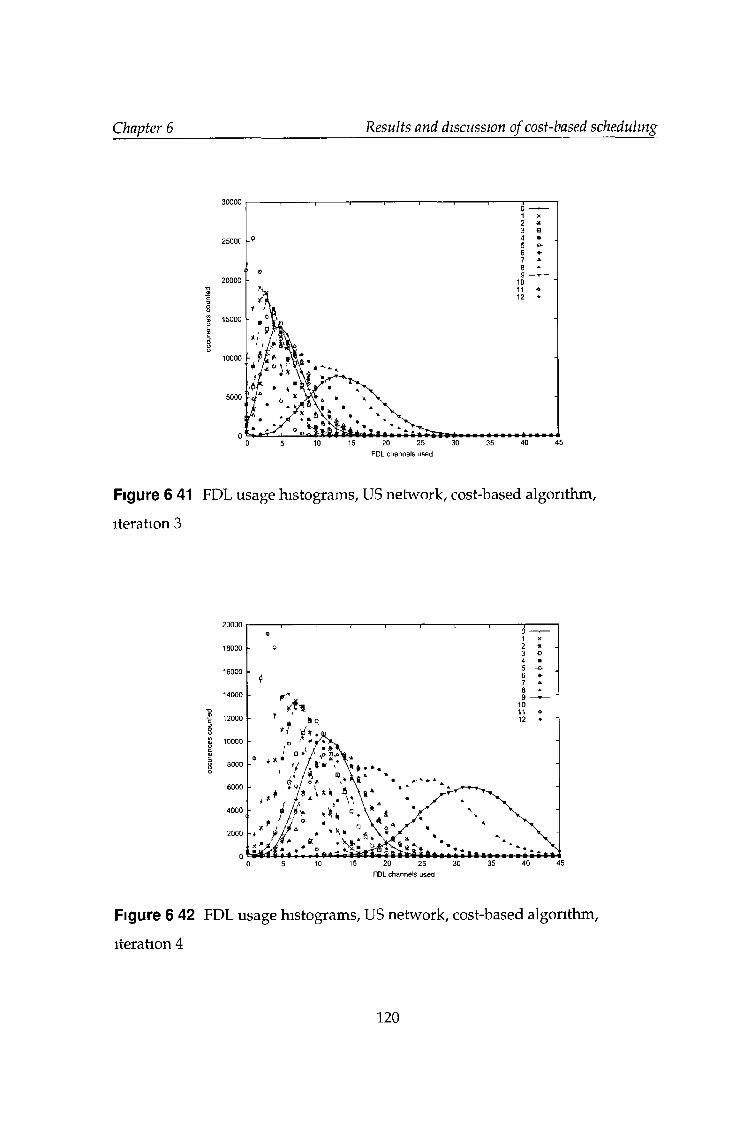
Chapter 6 Results and discussion of cost-based scheduling
Figure 6 41 FDL usage histograms, US network, cost-based algorithm,
iteration 3
Figure 6 42 FDL usage histograms, US network, cost-based algorithm,
iteration 4
120
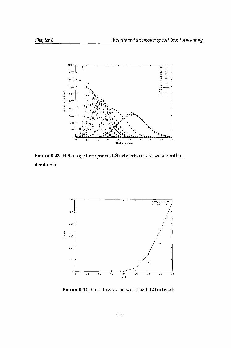
Chapter 6 Results and discussion of cost-based scheduling
FDL channels used
Figure 6 43 FDL usage histograms, US network, cost-based algorithm,
iteration 5
load
Figure 6 44 Burst loss vs network load, US network
121
Chapter 6 Results and discussion of cost-based scheduling
A few important observations can be made
• The nodes m the described network are very different in terms of handled
load, and number of outgoing links/channels Therefore, as the number of
FDL channels is identical in all nodes, m some cases care must be taken to
ensure that no bursts are lost because an FDL channel is unavailable m case
of contention, and m some cases it is not an issue, even when the FDL price
is set to 0
• The total loss ratio is averaged across the entire network In some links the
cost-based algorithm offers much better performance than LAUC-VF and
m some the performance of both algorithms is very similar (for example
if the link is overloaded) Therefore, the total measured performance gam
of the cost-based algorithm is lower than m the case of a single node and
symmetrical network simulations
6 3.3 Pan-European netw ork
Simulations analogous to those described m the previous section were performed
usmg a more complex network, shown in Fig 6 45 [96] It is a pan-European
network, defined m the COST 266 project [96-98]
There were 75 channels m each FDL bank, and its length was equal to one-
third of the burst length The offset time was uniformly distributed over the range
of seven burst lengths The simulation procedure was identical to that previously
described A traffic matrix based on the one provided m [96] was used and the
link sizes were adjusted to obtain loss ratios m the range of one percent in all
links
Fig 6 46 shows the burst loss ratios obtained in successive rounds of simu
lations and Fig 6 47-6 50 the correspondmg FDL usage histograms Finally, Fig
122
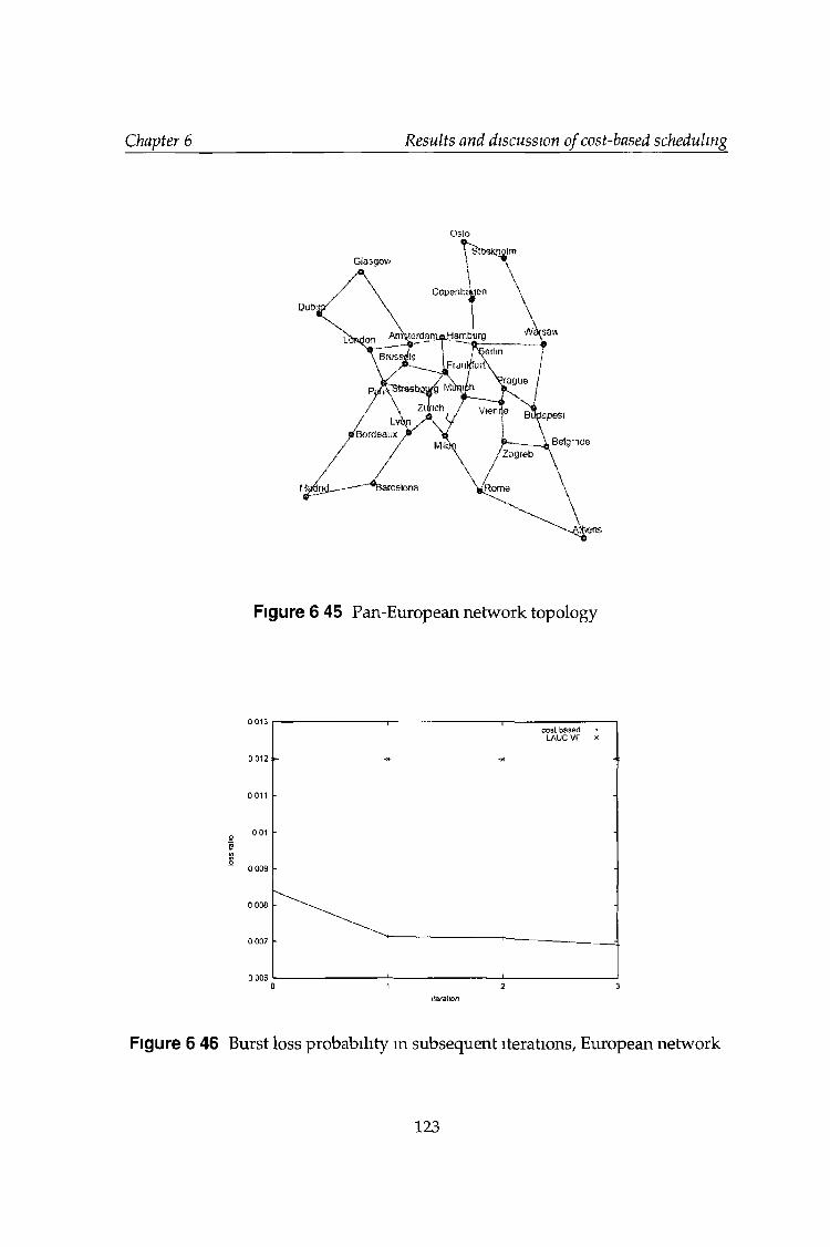
Chapter 6 Results and discussion of cost-based scheduling
Oslo
Figure 6 45 Pan-European network topology
ileralion
Figure 6 46 Burst loss probability in subsequent iterations, European network
123
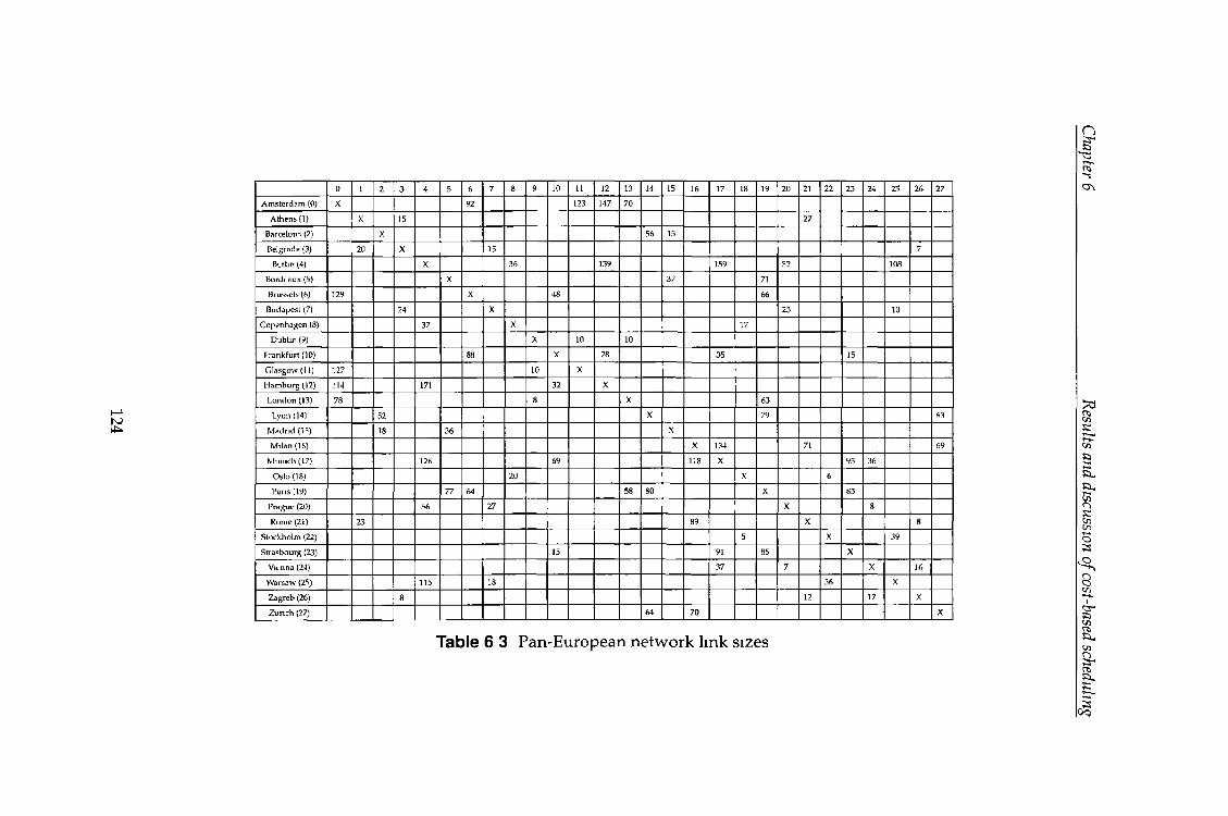
0 ! 2 3 4 5 6 7 8 9 10 11 12 13 14 15 16 17 18 19 20 21 22 23 24 25 26 27
Am sterdam (0) X 92 123 147 70
Athene (1) X 15 27
Barcelom (2) X 56 15
Belgrade (3) 20 X 15 7
Berlin (4) X 36 139 159 52 108
Bordeaux (5) X 37 71
Brussels (6) 129 X 48 66
Budapest (7) 24 X 25 10
Copenhagen (8) 37 X 17
Dublin (9) X 10 10
Frankfurt (10) 88 X 28 35 15
Glasgow (11) 127 10 X
Ham burg (12) 114 171 32 X
London (13) 78 8 X 63
Lyon (14) 52 X 79 63
M adrid ( l 1̂) 18 36 X
Milan (16) X 134 71 69
M unich (17) 126 69 118 X 95 36
Oslo (18) 20 X 6
Pans (19) 77 64 58 80 X 85
Prague (20) 56 27 X 8
Rome (21) 23 89 X 8
Stockholm (22) 5 X 39
Strasbourg (23) 15 91 85 X
Vienna (24) 37 7 X 16
W arsaw (2^) 115 18 36 X
Zagreb (26) 8 12 17 X
Zunch (27) 64 70 X
Table 6 3 Pan-European netw ork link sizes
Chapter 6
Results and discussion
of cost-based
scheduling
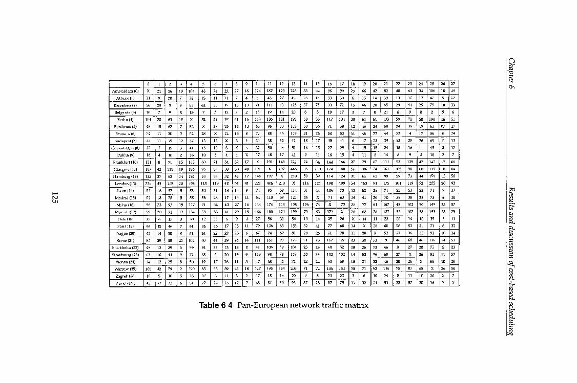
0 1 2 3 4 5 6 7 8 9 1U 11 12 13 14 15 16 17 18 19 20 21 22 23 24 25 26 27
A m sterdam (0) X 21 56 10 104 48 74 22 27 16 124 187 123 226 53 52 96 99 2d 66 42 82 48 63 34 106 10 45
A thens (1) 21 X 20 7 28 15 11 11 7 4 8 43 27 45 16 18 33 30 6 15 14 39 13 16 12 42 5 12
Barcelona (2) 56 20 X 9 63 62 30 19 15 10 71 111 63 125 57 75 93 72 15 46 30 85 29 44 25 79 10 33
B elgnde (3) 10 7 9 X 15 7 5 12 3 2 15 19 14 20 8 8 19 17 3 7 8 21 6 9 8 2 5 6
Berlin (4) 104 28 63 15 X 52 52 37 41 16 143 186 181 198 58 58 117 134 30 61 61 103 59 72 50 190 16 51
Bordeaux (5) 48 15 62 7 52 X 28 15 13 10 60 96 53 113 50 56 71 58 12 46 24 60 24 38 19 63 07 27
Brussels (6) 74 11 30 5 52 28 X 12 13 8 71 88 56 119 31 28 54 53 11 46 22 44 22 4 17 56 6 24
Budapest (7) 22 11 19 12 37 15 12 X 8 4 34 38 32 42 18 17 40 41 6 17 23 39 13 20 26 69 11 13
Copenhagen (8) 27 7 15 3 41 13 13 8 X 4 32 50 4t 51 14 15 27 29 9 15 15 24 18 16 11 45 3 12
Dublin (9) 16 4 10 2 16 10 8 4 4 X 17 48 17 41 9 11 16 15 4 11 6 14 8 9 5 18 2 7
F rankfurt (10) 124 8 71 15 143 60 71 34 32 17 X 191 148 221 74 64 144 166 27 79 67 111 53 129 47 147 17 68
Glasgow (11) 187 43 111 19 186 96 88 38 50 48 191 X 197 446 95 110 174 180 56 106 74 161 105 98 68 195 18 84
H am burg (12) 123 27 63 14 181 53 56 32 45 17 148 197 X 210 59 59 114 124 31 6? 62 99 59 73 44 159 15 50
London (13) 226 45 125 20 198 113 119 42 51 41 221 446 210 X 114 121 198 199 54 153 81 175 104 119 72 205 20 93
L>on (14) 53 16 57 8 58 50 31 18 14 9 74 95 59 114 X 44 106 73 13 52 28 71 25 53 22 71 9 37
M adrid (15) 52 18 75 8 58 56 28 17 15 11 64 110 59 121 44 X 74 63 14 41 26 70 28 38 22 72 8 28
M ihn(16) 96 33 93 19 117 71 54 40 27 16 144 174 114 198 106 74 X 173 25 77 61 167 48 102 50 14^ 23 87
M unich (17) 99 30 72 17 134 58 53 41 29 15 166 180 124 199 73 63 173 X 26 68 78 127 52 102 58 153 23 75
Oslo (18) 25 6 15 3 30 12 11 6 9 4 27 56 31 54 13 14 25 26 X 14 11 23 20 14 10 35 3 11
Paris (19) 66 15 46 7 61 46 46 17 15 11 79 106 65 153 52 41 77 68 14 X 28 60 26 52 21 71 6 32
Prague (21)) 42 14 30 8 61 24 22 23 15 6 67 74 62 81 28 26 61 78 11 28 X 52 23 36 32 92 10 24
Rome (21) 82 39 85 21 103 60 44 39 24 14 111 161 99 175 71 70 167 127 23 60 52 X 46 68 46 136 24 53
Stockholm (22) 48 13 29 6 ^9 24 22 13 18 8 53 105 59 104 25 28 48 52 20 26 23 46 X 27 20 75 5 23
Strasbourg (23) 63 16 44 9 72 38 4 20 16 9 129 98 73 119 53 38 102 102 14 52 36 68 27 X 26 82 11 57
Vienna (24) 34 12 25 8 SO 19 17 26 11 5 47 68 44 72 22 22 50 58 10 21 32 46 20 26 X 68 10 20
W arsaw (25) 106 42 79 2 190 63 56 69 45 18 147 195 159 205 71 72 145 153 35 71 92 136 75 82 68 X 26 56
Zagreb (26) 10 5 10 5 16 07 6 11 3 2 17 18 lo 20 9 8 23 23 3 6 10 24 5 11 10 26 X 7
7 u n c h (27) 45 12 33 6 51 27 24 13 12 7 68 84 50 93 37 28 87 75 11 32 24 53 23 57 20 56 7 X
Table 6 4 Pan-European network traffic matrix
Chapter 6 Results
and discussion
of cost-based
scheduling
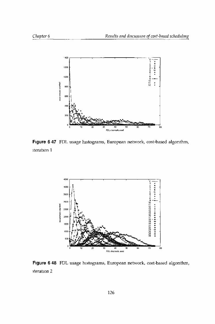
Chapter 6 Results and discussion of cost-based scheduling
Figure 6 47 FDL usage histograms, European network, cost-based algorithm,
iteration 1
30 40 50FDL channels used
Figure 6 48 FDL usage histograms, European network, cost-based algorithm,
iteration 2
126
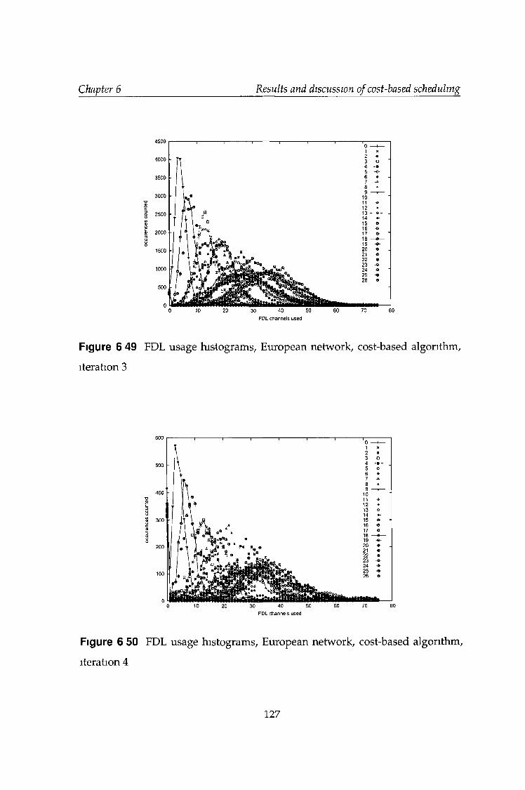
Chapter 6
Figure 6 49
iteration 3
Figure 6 50
iteration 4
Results and discussion of cost-based scheduling
FDL channels used
FDL usage histograms, European network, cost-based algorithm,
FDL channels used
FDL usage histograms, European network, cost-based algorithm,
127
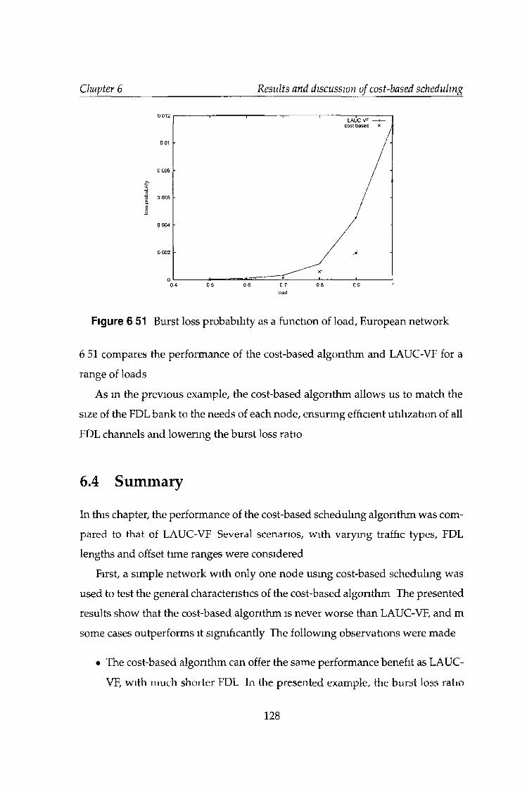
Chapter 6 Results and discussion of cost-based scheduling
Figure 6 51 Burst loss probability as a function of load, European network
6 51 compares the performance of the cost-based algorithm and LAUC-VF for a
range of loads
As m the previous example, the cost-based algorithm allows us to match the
size of the FDL bank to the needs of each node, ensuring efficient utilization of all
FDL channels and lowering the burst loss ratio
6.4 Summary
In this chapter, the performance of the cost-based schedulmg algorithm was com
pared to that of LAUC-VF Several scenarios, with varying traffic types, FDL
lengths and offset time ranges were considered
First, a simple network with only one node using cost-based schedulmg was
used to test the general characteristics of the cost-based algorithm The presented
results show that the cost-based algorithm is never worse than LAUC-VF, and m
some cases outperforms it significantly The following observations were made
• The cost-based algorithm can offer the same performance benefit as LAUC-
VF, with much shorter FDL In the presented example, the burst loss ratio
128
Chapter 6 Results and discussion of cost-based scheduling
of the cost-based algorithm with a FDL length equal to one-tenth of the
burst length was actually lower than that of LAUC-VF with ten times longer
FDL For very long FDLs the performance of both algorithms becomes very
similar However, the cost-based algorithm is never worse
• The cost-base algorithm consistently outperformed LAUC-VF, regardless of
the traffic type
• The relative performance of the cost-based algorithm is the best when the
range of possible offset times is relatively large
• The cost-based algorithm can effectively utilize FDL banks of much larger
sizes than LAUC-VF, and even though the algorithms converge for smaller
banks, is never worse
An idea of a FDL usage histogram was mtroduced, and those histograms were
used to explam the relationship between the initial FDL price and burst loss ratio,
and the relative performance of the cost-based algorithm as compared to LAUC-
VF
In the next part of this chapter, the capability of the cost-based algorithm to
match the needs of a node with its available FDL bank was tested m more com
plex scenarios The first simulation mvolved a ring network of six nodes As the
network was symmetrical, identical initial FDL price could be used in all nodes
The results were similar to those obtamed for a smgle node - again, the cost-based
algorithm offered improved performance, especially for large FDL bank sizes
Finally, two realistic network topologies were simulated a US NFS network,
and a COST 266 pan-European network In this case the FDL prices had to be
adjusted m each node individually, based on the FDL usage histograms The
simulations were performed in rounds, until no further improvement could be
achieved In both networks, the cost-based algorithm offered better performance
than LAUC-VF The difference, while not as big as m previous simulations, was
still significant
129
Chapter 7
Results and discussion of
cost-based burst dropping
A cost-based intentional burst dropping technique was introduced in Section
4 4 3 In this chapter simulations comparing its performance with that of random
burst dropping technique will be presented
7.1 Introduction
Let us consider a case with two traffic classes high and low priority class When
no bursts are intentionally dropped, then the loss ratio in both classes will be
identical However, discarding a certain proportion of low priority bursts will
improve the loss ratio in the high priority class Fig 7 1 presents such a case At
the starting point, the loss probability m both traffic classes is equal to PO The loss
ratio m the high priority class can then be decreased, but at a price of mcreasmg
the loss ratio experienced by the low priority class Fig 7 1 shows curves illus
trating this trade-off for two algorithms, denoted (a) and (b) Decreasmg the loss
ratio m the high priority class to PI requires mcreasmg the loss ratio m the low
priority class to either Pia or P\b, depending on the algorithm used Obviously, it
is desirable to use an algorithm where this additional increase is the smallest In
other words, the more concave the curve, the better the burst dropping algorithm
A random droppmg algorithm discards bursts blindly, without trying to as
sess the probability that a given burst will interfere with other bursts The cost-
based algorithm, on the other hand, uses the cost function to only drop those
130
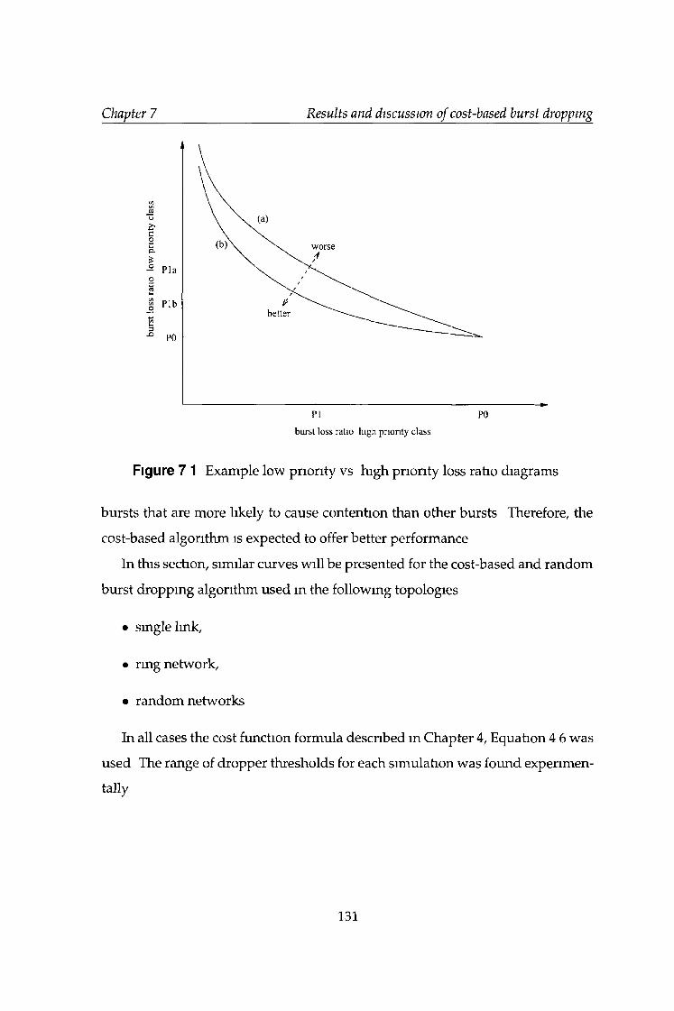
Chapter 7 Results and discussion of cost-based burst dropping
burst loss ratio high priority class
Figure 7 1 Example low priority vs high priority loss ratio diagrams
bursts that are more likely to cause contention than other bursts Therefore, the
cost-based algorithm is expected to offer better performance
In this section, similar curves will be presented for the cost-based and random
burst dropping algorithm used m the following topologies
• smgle lmk,
• ring network,
• random networks
In all cases the cost function formula described m Chapter 4, Equation 4 6 was
used The range of dropper thresholds for each simulation was found expenmen-
tally
131
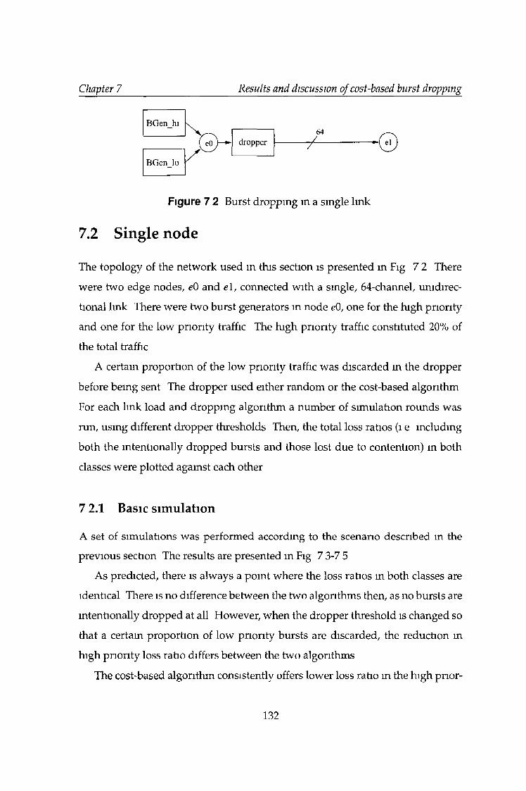
Chapter 7 Results and discussion of cost-based burst dropping
Figure 7 2 Burst dropping m a single link
7.2 Single node
The topology of the network used in this section is presented in Fig 7 2 There
were two edge nodes, eO and e l, connected with a single, 64-channel, unidirec
tional link There were two burst generators m node eO, one for the high priority
and one for the low priority traffic The high priority traffic constituted 20% of
the total traffic
A certain proportion of the low priority traffic was discarded in the dropper
before being sent The dropper used either random or the cost-based algorithm
For each link load and dropping algorithm a number of simulation rounds was
run, using different dropper thresholds Then, the total loss ratios (i e including
both the intentionally dropped bursts and those lost due to contention) in both
classes were plotted agamst each other
7 2.1 Basic sim ulation
A set of simulations was performed according to the scenario described in the
previous section The results are presented in Fig 7 3-7 5
As predicted, there is always a pomt where the loss ratios m both classes are
identical There is no difference between the two algorithms then, as no bursts are
intentionally dropped at all However, when the dropper threshold is changed so
that a certain proportion of low priority bursts are discarded, the reduction in
high priority loss ratio differs between the two algorithms
The cost-based algorithm consistently offers lower loss ratio m the high pnor-
132
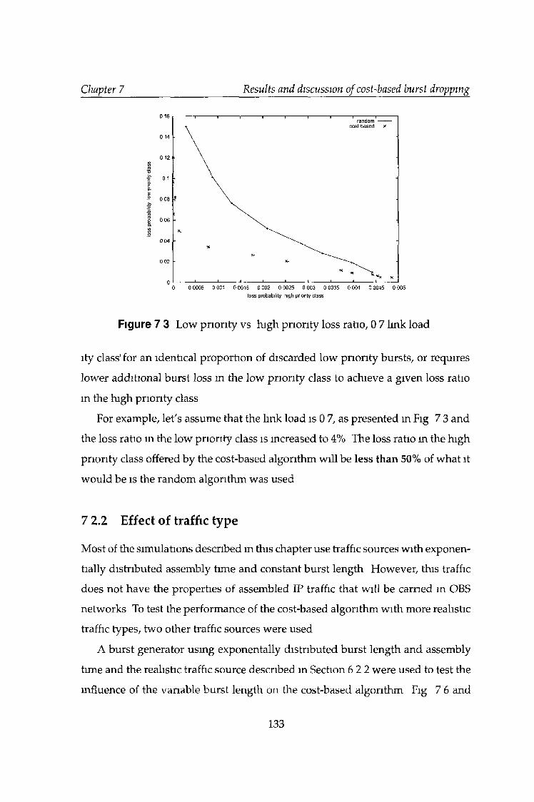
Chapter 7 Results and discussion of cost-based burst dropping
loss probability high priority class
Figure 7 3 Low priority vs high priority loss ratio, 0 7 link load
lty class' for an identical proportion of discarded low priority bursts, or requires
lower additional burst loss in the low priority class to achieve a given loss ratio
in the high priority class
For example, let's assume that the link load is 0 7, as presented in Fig 7 3 and
the loss ratio in the low priority class is increased to 4% The loss ratio in the high
priority class offered by the cost-based algorithm will be less than 50% of what it
would be is the random algorithm was used
7 2.2 Effect of traffic type
Most of the simulations described m this chapter use traffic sources with exponen
tially distributed assembly time and constant burst length However, this traffic
does not have the properties of assembled IP traffic that will be carried in OBS
networks To test the performance of the cost-based algorithm with more realistic
traffic types, two other traffic sources were used
A burst generator using exponentally distributed burst length and assembly
time and the realistic traffic source described in Section 6 2 2 were used to test the
influence of the variable burst length on the cost-based algorithm Fig 7 6 and
133
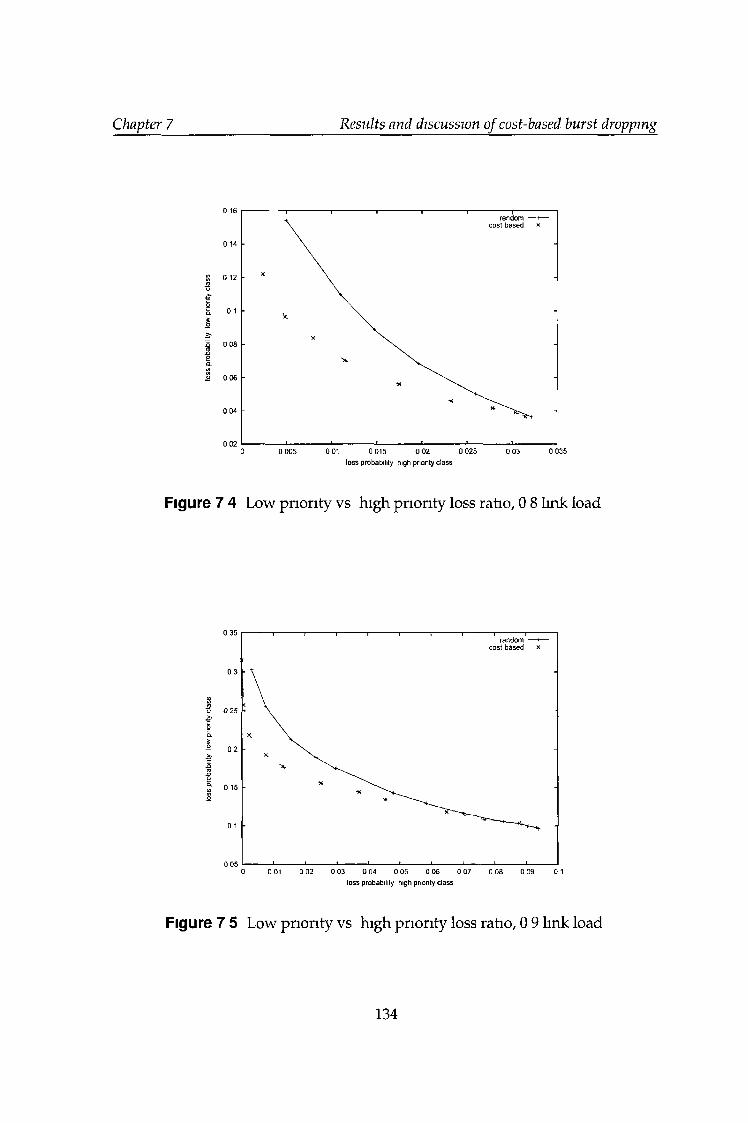
Chapter 7 Results and discussion of cost-based burst dropping
loss probability high priority class
Figure 7 4 Low priority vs high priority loss ratio, 0 8 link load
loss probability high priority class
Figure 7 5 Low priority vs high priority loss ratio, 0 9 link load
134
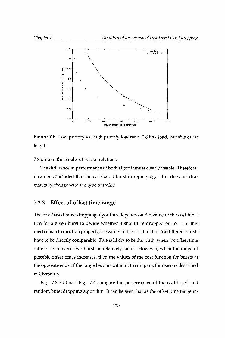
Chapter 7 Results and discussion of cost-based burst dropping
loss probability high priority class
Figure 7 6 Low priority vs high priority loss ratio, 0 8 link load, variable burst
length
7 7 present the results of this simulations
The difference in performance of both algorithms is clearly visible Therefore,
it can be concluded that the cost-based burst droppmg algorithm does not dra
matically change with the type of traffic
7 2 3 Effect of offset tim e range
The cost-based burst droppmg algorithm depends on the value of the cost func
tion for a given burst to decide whether it should be dropped or not For this
mechamsm to function properly, the values of the cost function for different bursts
have to be directly comparable This is likely to be the truth, when the offset time
difference between two bursts is relatively small However, when the range of
possible offset times increases, then the values of the cost function for bursts at
the opposite ends of the range become difficult to compare, for reasons described
m Chapter 4
Fig 7 8-7 10 and Fig 7 4 compare the performance of the cost-based and
random burst dropping algorithm It can be seen that as the offset time range m-
135
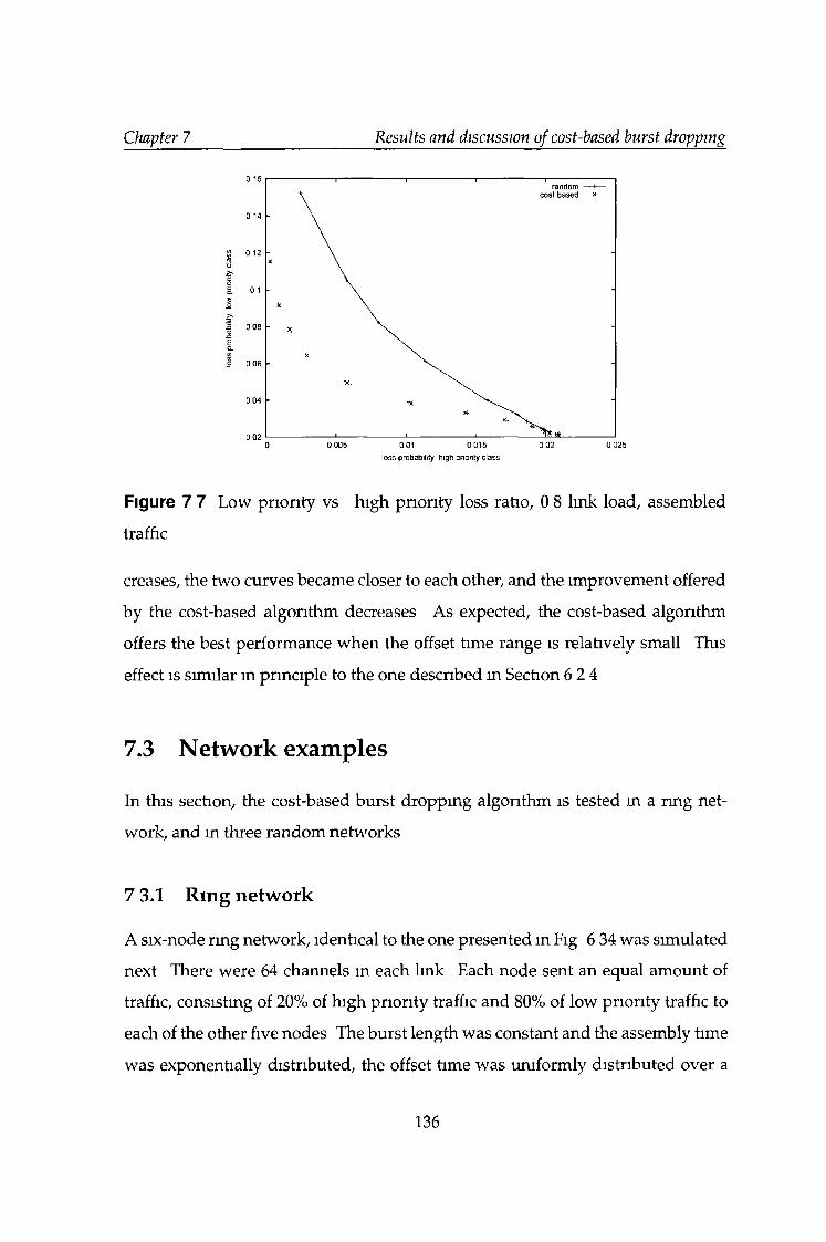
Chapter 7 Results and discussion of cost-based burst dropping
loss probability high prionty class
Figure 7 7 Low priority vs high priority loss ratio, 0 8 link load, assembled
traffic
creases, the two curves became closer to each other, and the improvement offered
by the cost-based algorithm decreases As expected, the cost-based algorithm
offers the best performance when the offset time range is relatively small This
effect is similar m principle to the one described in Section 6 2 4
7.3 Network examples
In this section, the cost-based burst dropping algorithm is tested m a ring net
work, and m three random networks
7 3.1 R ing netw ork
A six-node rmg network, identical to the one presented in Fig 6 34 was simulated
next There were 64 channels in each lmk Each node sent an equal amount of
traffic, consistmg of 20% of high priority traffic and 80% of low priority traffic to
each of the other five nodes The burst length was constant and the assembly time
was exponentially distributed, the offset time was uniformly distributed over a
136
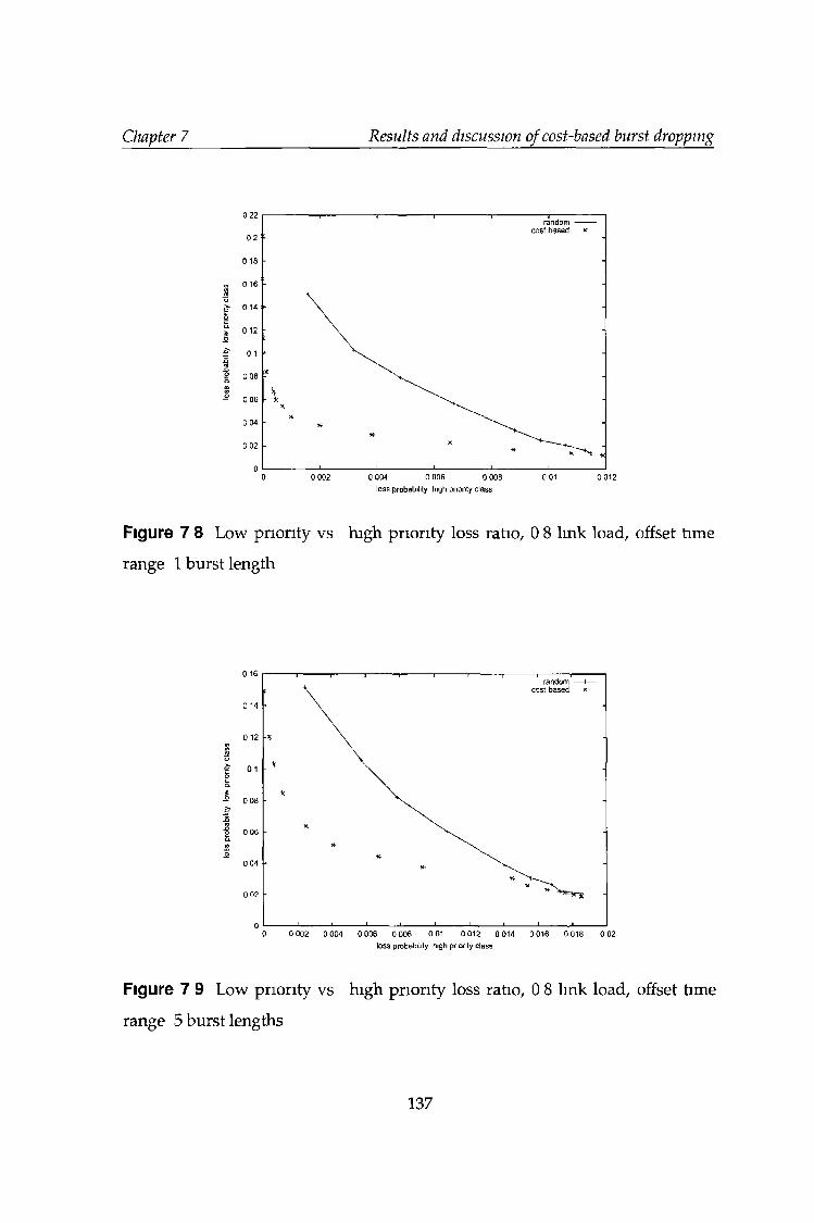
Chapter 7 Results and discussion of cost-based burst dropping
less probability high priority class
Figure 7 8 Low priority vs high priority loss ratio, 0 8 link load, offset time
range 1 burst length
loss probability high priority class
Figure 7 9 Low priority vs high priority loss ratio, 0 8 link load, offset time
range 5 burst lengths
137
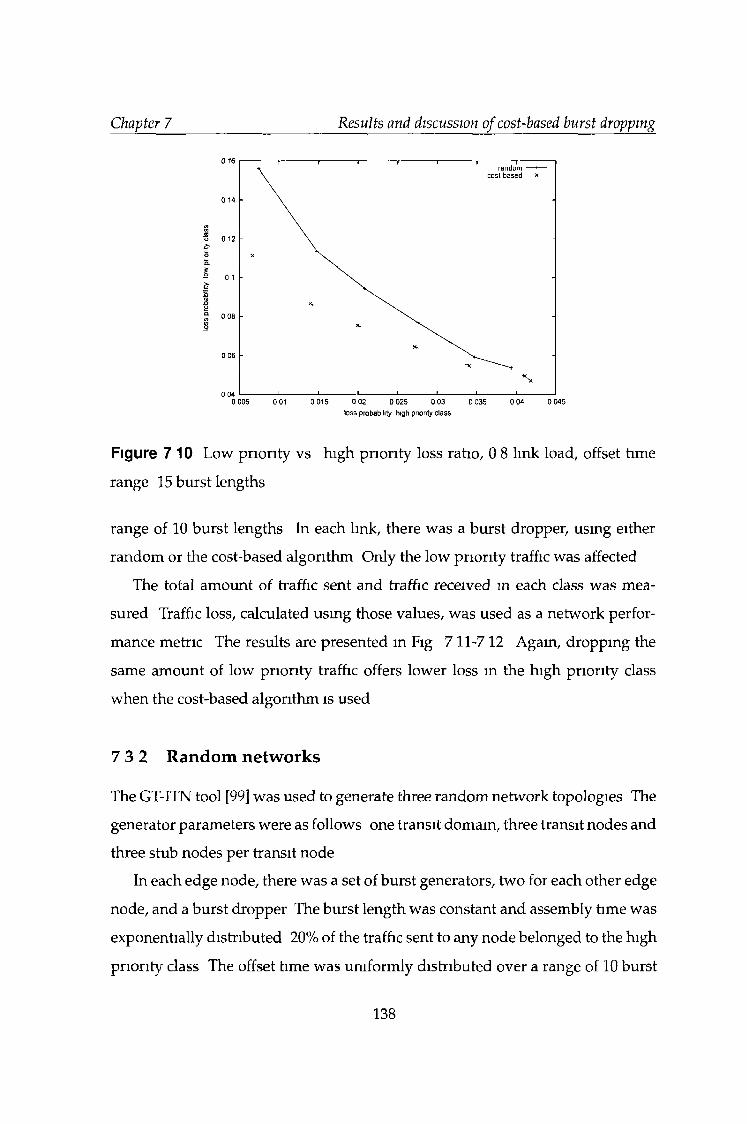
Chapter 7 Results and discussion of cost-based burst dropping
toss probability high priority class
Figure 710 Low priority vs high priority loss ratio, 0 8 link load, offset time
range 15 burst lengths
range of 10 burst lengths In each link, there was a burst dropper, usmg either
random or the cost-based algorithm Only the low priority traffic was affected
The total amount of traffic sent and traffic received in each class was mea
sured Traffic loss, calculated usmg those values, was used as a network perfor
mance metric The results are presented in Fig 7 11-7 12 Again, dropping the
same amount of low priority traffic offers lower loss m the high priority class
when the cost-based algorithm is used
7 3 2 Random ne tw orks
The GT-ITN tool [99] was used to generate three random network topologies The
generator parameters were as follows one transit domain, three transit nodes and
three stub nodes per transit node
In each edge node, there was a set of burst generators, two for each other edge
node, and a burst dropper The burst length was constant and assembly time was
exponentially distributed 20% of the traffic sent to any node belonged to the high
priority class The offset time was uniformly distributed over a range of 10 burst
138
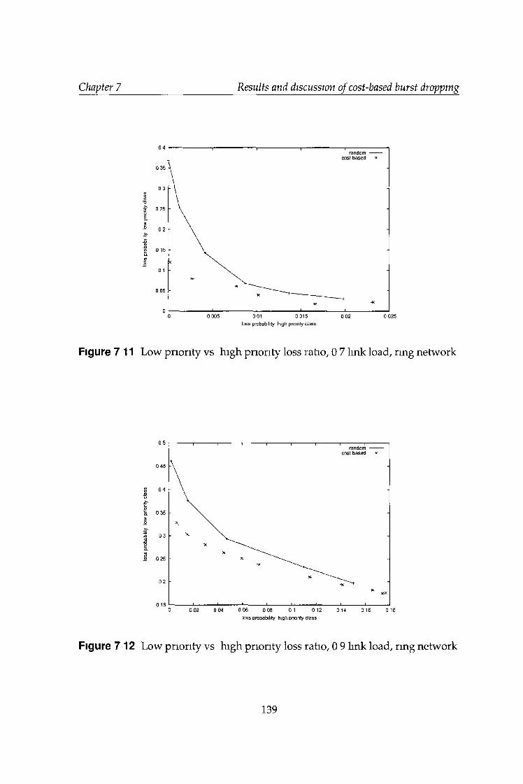
Chapter 7 Results and discussion of cost-based burst dropping
loss probability high priority class
Figure 7 11 Low priority vs high priority loss ratio, 0 7 link load, ring network
loss probability high priority class
Figure 712 Low priority vs high priority loss ratio, 0 9 link load, ring network
139
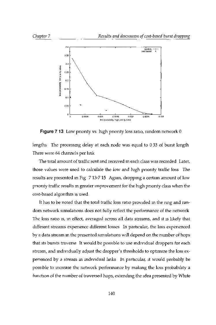
Chapter 7 Results and discussion of cost-based burst dropping
loss probability high priority class
Figure 7 13 Low priority vs high priority loss ratio, random network 0
lengths The processmg delay at each node was equal to 0 33 of burst length
There were 64 channels per lmk
The total amount of traffic sent and received m each class was recorded Later,
those values were used to calculate the low and high priority traffic loss The
results are presented in Fig 7 13-7 15 Again, droppmg a certain amount of low
priority traffic results m greater improvement for the high priority class when the
cost-based algorithm is used
It has to be noted that the total traffic loss ratio provided m the rmg and ran
dom network simulations does not fully reflect the performance of the network
The loss ratio is, in effect, averaged across all data streams, and it is likely that
different streams experience different losses In particular, the loss experienced
by a data stream in the presented simulations will depend on the number of hops
that its bursts traverse It would be possible to use individual droppers for each
stream, and individually adjust the dropper's thresholds to optimize the loss ex
perienced by a stream in individual links In particular, it would probably be
possible to increase the network performance by makmg the loss probability a
function of the number of traversed hops, extending the idea presented by White
140
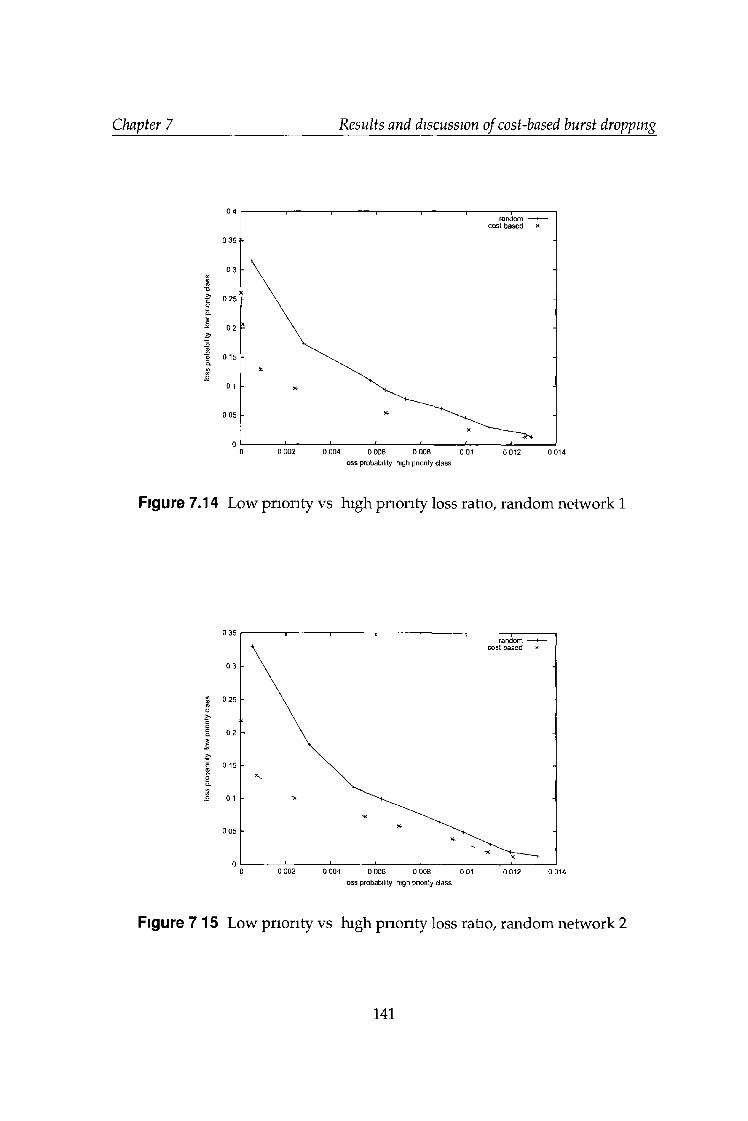
Chapter 7 Results and discussion of cost-based burst dropping
loss probability high priority class
Figure 7.14 Low priority vs high priority loss ratio, random network 1
loss probability high pnonty class
Figure 715 Low priority vs high priority loss ratio, random network 2
141
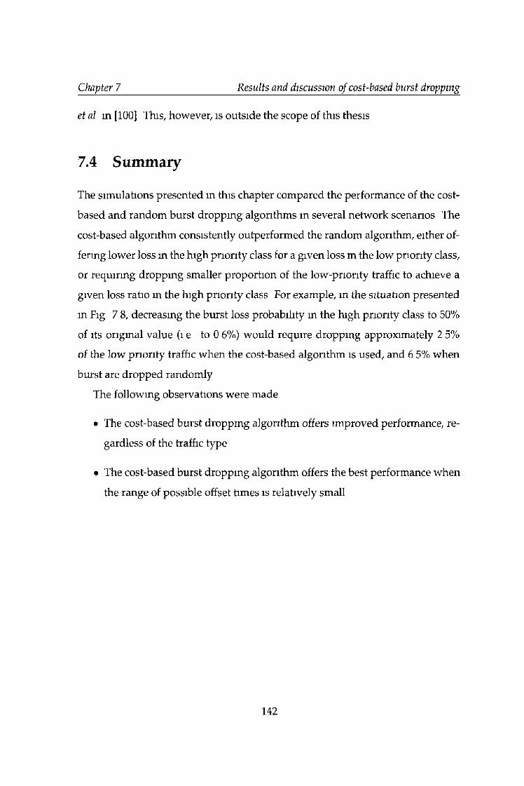
Chapter 7 Results and discussion of cost-based burst dropping
et al in [100] This, however, is outside the scope of this thesis
7.4 Summary
The simulations presented in this chapter compared the performance of the cost-
based and random burst dropping algorithms m several network scenarios The
cost-based algorithm consistently outperformed the random algorithm, either of
fering lower loss in the high priority class for a given loss m the low priority class,
or requiring dropping smaller proportion of the low-priority traffic to achieve a
given loss ratio m the high priority class For example, in the situation presented
in Fig 7 8, decreasing the burst loss probability in the high priority class to 50%
of its original value (i e to 0 6%) would require dropping approximately 2 5%
of the low priority traffic when the cost-based algorithm is used, and 6 5% when
burst are dropped randomly
The following observations were made
• The cost-based burst dropping algorithm offers improved performance, re
gardless of the traffic type
• The cost-based burst dropping algorithm offers the best performance when
the range of possible offset times is relatively small
142
Chapter 8
Conclusions
Optical Burst Switching (OBS) is a promising new paradigm, filling the gap be
tween optical circuit switching (OCS) and optical packet switching (OPS). A burst-
switched network can fully utilize the enormous bandwidth of an optical fibre,
while offering higher granularity than OCS networks. At the same time, the hard
ware requirements of an OBS network are lower than in the case of OPS. This
makes them an attractive choice for the future Internet.
In Optical Burst-Switched networks reservations are made in advance. This
makes the alignment of bursts within channels a very important issue. Depend
ing on this alignment, the available bandwidth may become more or less frag
mented, resulting in higher or lower loss probability for future bursts. In this
thesis a way of judging this alignment in a numerical way is presented, along
with its possible applications.
A cost function value can be used to predict the probability that allocating a
burst will cause a future burst to be dropped due lo a contention. This thesis
provided a formal definition of a cost function. Then a theoretical analysis of
the probability of a given burst causing a contention was presented, and a cost
function formula based on it was proposed.
The idea of a cost function was used to design a scheduling algorithm. Schedul
ing a burst requires using some of the resources available in the node. Those re
sources may include outgoing links, fiber delay lines or wavelength converters.
By assigning a virtual price to each of those resources a lowest-priced combina
tion can be then chosen.
The simulation results presented in this thesis were obtained using an OBS
143
Chapter 8 Conclusions
extension to the well-known ns-2 simulator The robust and efficient underlying
ns-2 simulation engine coupled with an extensive set of OBS classes provided a
powerful simulation tool, capable of simulating an OBS network as a part of IP
network, or on its own, for better efficiency
Presented simulation results prove that the cost-based algorithm can offer im
proved performance when compared with LAUC-VF Depending on the simula
tion parameters, the difference can reach an order of magnitude, especially for
low loads In the situation presented in Fig 6 19, when the link load is equal
to 0 5, the loss probability offered by the cost-based algorithm is over ten times
smaller than that of LAUC-VF (0 0021% vs 0 0332%) In some cases the perfor
mance of both algorithms becomes similar, but the cost-based algorithm is never
worse
The performance of the cost-based scheduling algorithm as a function of FDL
length was studied next It was found that the performance of both LAUC-VF and
the cost-based algorithm improves as a function of FDL length, and converges for
very long FDLs However, the difference is very significant for shorter delay lines
As demonstrated m Fig 6 30, the cost-based algorithms usmg a relatively short
FDL (one-tenth of the burst length) outperforms LAUC-VF with ten times longer
FDL
Later, it was demonstrated that by assigning an appropriate initial FDL price,
FDL banks of varying sizes can be effectively utilized by a node This was done
first by varymg the size of an FDL bank m a smgle node or a rmg network In
both cases, the performance of LAUC-VF improved only until the size of the FDL
bank reached approximately 5 channels and then levelled off The cost-based
algorithm, on the other hand, was capable of utilizing additional FDL channels,
For a large FDL bank, the loss ratio of LAUC-VF was approximately twice as big
as that of the cost-based algorithm, as shown m Fig 6 31 (1 3% vs 0 7%) and 6 35
(2% vs 11%)
Then, FDL banks of identical size were used m two larger networks The first
144
Chapter 8 Conclusions
topology was based on the formes National Science Foundation network, and
the other one on the pan-European network defined m the COST 266 project In
both cases, by adjustmg the FDL price in each node individually, it was possible
to achieve lower burst loss ratio than m the case of LAUC-VF, especially for low
loads For example, the overall loss ratio in the pan-European network for a load
of 0 5 times the base load, was more than six times larger when LAUC-VF was
used The difference decreased for higher loads, likely due to overloading of a
few links in the network
Several Quality of Service (QoS) schemes use the idea of early or mtentional
burst dropping m low priority classes to reduce loss probability experienced by
high priority bursts A cost-based burst dropping algorithm that only drops
bursts when the value of the cost function exceeds a certain threshold was pro
posed As the cost function value reflects the probability that a given burst will
cause a contention, this algorithm offers better performance than a random one
Simulation results were presented for several scenanos
First, a single-link topology was used to mvestigate the effects of traffic type
and offset time range on the performance of the cost-based burst dropping algo
rithm It was found that the impact of the traffic type was not very significant,
and that the performance of the cost-based algorithm improved when the range
of possible offset times was relatively small For example, when the range of pos
sible offset times was equal to one burst length, increasing the burst loss ratio m
the low priority class from original 1 2% to 4% resulted m approximately 0 8%
loss ratio m the high priority class when bursts were dropped randomly, and less
than 0 2% when the cost-based burst dropping algorithm was used
Then, the cost-based burst droppmg algorithm was tested m a rmg network
and three random networks Again, its performance was better than m the case of
random burst droppmg In one of the random networks, decreasing the burst loss
in the high priority class to nearly zero required droppmg approximately 10% of
low priority bursts using the cost-based burst droppmg algorithm To achieve
145
Chapter 8 Conclusions
the same effect by random burst droppmg it was necessary to drop 35% of low
priority bursts (Fig 7 13)
In conclusion, the cost-based algorithms offer improved performance com
pared to standard solutions Depending on the network parameters, the differ
ence may be very significant, and the cost-based algorithms are never worse, even
in unfavorable conditions
8.1 Future work
The proposed cost function formulas only consider the alignment of bursts within
one channel In particular, the state of other channels and burst destinations are
not taken mto account Using this information it is reasonable to expected a signif
icant performance benefit, as the resulting algorithm could tend to group bursts
with the same destination address m one channel, or reduce their overlap It
would be particularly interesting to investigate the performance of such an algo
rithm in a non-void filling system
All the simulations presented m this thesis used fixed-length FDLs It may be
possible to use several FDLs of varying length, or to use contmuous delays (at
the network edge) In the latter case, the cost of delaying a burst would probably
depend on the amount of memory used, and the duration of its use
Finally, the idea of cost-based scheduling can be used m any system, where
resources have to be reserved in advance Systems where reservations can be
delayed at a certain cost are particularly suitable For example, if a large amount
of experimental data has to be processed, the data can be stored, but the available
disk space may be limited A cost-based algorithm could balance the need to use
the CPU time m an efficient manner and to minimize delay
146
Bibliography
[1] LG Roberts Beyond Moore's law Internet growth trends IEEE Computer,
vol 33, no l , p 117,2000
[2] Scientists at Lucent Technologies' Bell Labs calcu
late theoretical limits of fiber optic communications,
http / / www lucent com/ press /0601 /010628 bla html, retrieved on 02
Dec 2005
[3] T Battestilli and H Perros Optical Burst Switching A Survey Technical
report, Technical report TR-2002-10, NC State University, Computer Science
Department, July 2002
[4] Generalized Multi-Protocol Label Switching (GMPLS) Architecture
rfc3945
[5] Generalized Multi-Protocol Label Switching (GMPLS) Signaling Functional
Description rfc3471
[6] Will E Leland and Murad S Taqq and Walter Willinger and Daniel V Wil
son On the self-similar nature of Ethernet traffic In Proceedings of ACM
SIGCOMM, San Francisco, California, 1993
[7] J Beran and R Sherman and M S Taqqu and W Willinger Long-Range
Dependence in Variable-Bit-Rate Video Traffic IEEE Transactions on Com
munications, vol 43, no 213/4, pp 1566-1579,1995
147
Bibliography
[8] L Xu, H Perros, and G Rouskas Techniques for Optical Packet Switching
and Optical Burst Switching IEEE Communications, Jan 2001
[9] C Qiao and M Yoo Optical burst switching (OBS) - a new paradigm for an
Optical Internet Journal of High Speed Networks, vol 8, no 1, pp 69-84,1999
[10] T Battestilli and H Perros An introduction to optical burst switching,
IEEE Communications Optical Magazine, S10S15, Vol 41,2003
[11] S R Amstutz Burst switching-An introduction IEEE Communications
Magazine, vol 21, no 8, pp 36-42,1983
[12] S R Amstutz Burst switching-An update IEEE Communications Magazine,
vol 21, no 6, pp 50-57,1989
[13] C Gauger, K Dolzer,J Spath, S Bodamer Service Differentiation in Optical
Burst Switching Networks ITG Fachtagung Photonische Netze pp 124-132,
2001
[14] E A Varvangos and V Sharma The Ready-to-Go Virtual Circuit Proto
col A Loss-Free Protocol for Multigigabit Networks Using FIFO Buffers
IEEE/ACM Transactions on Networking, vol 5, no 5, October 1997
[15] I Widjaja Performance Analysis of Burst Admission Control Protocols
IEEE Proceedings on Communications, vol 142, no 1, pp 7-14, Feb 1995
[16] Mills, DL, C G Boncelet, JG Elias, PA Schragger, A W Jackson and A
Thyagarajan Fmal report on the Highball Project In Electrical Engineeing
Department Report 95-4-1, University of Delaware, April 1995
[17] J Y Wei and R I McFarland Jr Just-in-time signaling for WDM optical
burst switching networks IEEE Journal of Lightwave Technology, vol 18, pp
2091
[18] The JumpStart project http / /jum pstart anr mcnc org
148
Bibliography
[19] I Baldine, H Perros, G Rouskas and D S Stevenson JumpStart A Just-in-
Time Signaling Architecture for WDM Burst-Switched Networks In IEEE
Communications, 40(2), pp 82-89, 2002
[20] J S Turner Terabit burst switching Journal of High Speed Networks, vol 8,
pp 3-16,1999
[21] J Turner Terabit burst switching progress report (9/98-12/98) Technical
report, Washington University at St Louis Technical Report, 1998
[22] J Teng, G Rouskas A Comparison of the JIT, }ET, and Horizon Wavelength
Reservation schemes on a single OBS node In The First International Work
shop on Optical Burst Switching, Dallas, Texas, Oct 2003
[23] M Yoo and C Qiao Just-enough-time(JET) a high speed protocol for
bursty traffic m optical networks IEEE/LEOS Technologies for a Global In
formation Infrastructure, 1997
[24] K Dolzer and C Gauger and J Spth and S Bodamer Evaluation of Reser
vation Mechanisms for Optical Burst Switching
[25] J Teng, G Rouskas A Detailed Analysis and Performance Comparison of
Wavelength Reservation Schemes for Optical Burst Switched Networks
Photonic Network Communications, vol 9, no 3, pp 311-335, May 2005
[26] A Ge, F Callegati, L S Tamil On optical burst switching and self-similar
traffic IEEE Communications Letters, vol 4 no 3, 2000
[27] G Hu, K Dolzer, C M Gauger Does burst assembly really reduce the self-
similarity? In Proceedings of Optical Fiber Communication Conference (OFC
2003)
[28] X Yu, Y Chen and C Qiao A Study of Traffic Statistics of Assembled Burst
Traffic m Optical Burst Switched Networks In Proceedings ofOpticomm 2002
149
Bibliography
[29] X Cao and J Li and Y Chen and C Qiao Assembling TCP/IP Packets in
Optical Burst Switched Networks In Proceeding of IEEE Globecom, 2002
[30] T Tachibana, T Ajima and S Kasahara Round-Robin Burst Assembly and
Constant Transmission Scheduling for Optical Burst Switchmg Networks
In Proceedings of IEEE GLOBECOM 2003
[31] Klaus Dolzer Assured Horizon - A new Combmed Framework for Burst
Assembly and Reservation m Optical Burst Switched Networks In Proceed
ings of the European Conference on Networks and Optical Communications (NOC
2002)
[32] VM Vokkarane,K Haridoss, and J P Jue Threshold-Based Burst Assembly
Policies for QoS Support in Optical Burst-Switched Networks In Proceed
ings of SPIE OptiComm 2002
[33] S Oh, H Ha Hong, M Kang A Data Burst Assembly Algorithm m Optical
Burst Switchmg Networks ETRI Journal, vol 24, no 4pp 311-322, Aug 2002
[34] V Vokkarane and Q Zhang and J Jue and B Chen Generalized Burst
Assembly and Schedulmg Techniques for QoS Support m Optical Burst-
Switched Networks In Proceedings of IEEE Globecom 2002
[35] T Hashiguchi, X Wang, H Monkawa and T Aoyama Burst Assembly
Mechanism with Delay Reduction for OBS Networks In Proceedings of
COIN/ACOFT 2003
[36] S A N Ostnng and H Sinsena The influence of long-range dependence
on traffic prediction In Proceedings of ICC 2001
[37] A Sang and San-qi Li A predictability analysis of network traffic In Pro
ceedings oflNFOCOM 2000
[38] A Adas Supporting real time VBR video using dynamic reservation based
on linear prediction In Proceedings of IEEE INFOCOM 96
150
Bibliography
[39] D Morato, J Aracil,L Angel Diez,M Izal and Eduardo Magana On linear
prediction of Internet traffic for packet and burst switching networks In
Proceedings oflCCCN 2001, October
[40] T W Yeow, E Law and A Goldenberg MEMS Optical Switches IEEE Com
munications Magazine, pp 158-163,2001
[41] C Guillemot, M Renaud, P Gambim, C Janz, I Andonovic, R Bauknecht,
B Bostica, M Burzio, F Callegati, M Casom, D Chiarom, F Clerot, S L
Damelsen, F Dorgeuille, A Dupas, A Franzen, P B Hansen, D K Hunter,
A Kloch, R Krahenbuhl, B Lavigne, A Le Core, C Raffaelli, M Schilling,
J Simon and L Zucchelh Transparent Optical Packet Switchmg The Eu
ropean ACTS KEOPS Project Approach Journal of Lightwave Technology, vol
16, no 12, pp 2117-2134, Dec 1998
[42] D Chiarom, B Lavigne, A Jourdan, M Sotom, L Hamon, C Chauzat, J
Jacquinot, A Barosso, T Zami, F Dorgeuille, C Janz, J Emery, E Grard
and M Renaud Physical and Logical Validation of a Network Basen on
All-Optical Packet Switching Systems Journal of Lightwave Technology, vol
16, no 12, pp 2255-2264, Dec 1998
[43] H Buchta,E Patzak,J Samter, C Gauger Maximal and Effective Through
put of Optical Switchmg Nodes for Optical Burst Switchmg In Beitrge zur
4 ITG-Fachtagung Photomsche Netze, 2003
[44] M Renaud, M Bachmann, M Erman Semiconductor optical space
switches IEEE Journal of Selected Topics in Quantum Electronics, Vol 2, No 2,
June 1996, pp 277-288
[45] M J Potasek All-Optical Switchmg for High Bandwidth Optical Network
Optical Networks Magazine, Vol 3, No 6, November/December 2002, pp 30- 43
151
Bibliography
[46] H Feng, E Patzak, J Samter Size and Cascadability Limits of SOA based
Burst Switching Nodes In Proc ECOC 2002, September 2002, Copenhagen,
Denmark
[47] Kapil V Shrikhande, I M White, M S Rogge, F-T An, A Srivatsa, E S
Hu, S S-H Yam and Leonid G Kazovsky Performance Demonstration of
a Fast-Tunable Transmitter and Burst-Mode Packet Receiver for HORNET
In Proc OFC 2001, Paper ThG2
[48] M Kauer, M Girault,J Leuthold, J H onthaas,0 Pellegri, C Goullancourt,
M Zirngibl 16-Channel Digitally Tunable Packet Switchmg Transmitter
with Sub-Nanosecond Switching Time In IEEE Photonics Technology Letters,
vol 15, no 3, March 2003
[49] J E Simsarian, A Bhardwa], K Dreyer, J Gripp, O Lazmcka, K Sherman,
Y Su, C Webb, L Zhang and M Zirngibl A Widely Tunable Laser Trans
mitter with Fast, Accurate Switchmg Between All Channel Combinations
In Proc ECOC 2002, September 2002, Copenhagen, Denmark
[50] T Durhuus, B Mikkelsen, C Joergensen, S L Damelsen, and K E Stubk-
jaer All-Optical Wavelength Conversion by Semiconductor Optical Am
plifiers IEEE Journal of Lightwave Technology, Vol 14, No 6, June 1996, pp
942-954
[51] C Dragone An n n optical multiplexor using a planar arrangment of two
star couplers IEEE Photonic Technology Letters, vol 6, pp 812815,1991
[52] J Ramamirtham, J Turner and J Friedman Design of Wavelength Con
verting Switches for Optical Burst Switchmg IEEE Journal on Selected Areas
In Communications, vol 21, No 7,pp 1122-1132, September 2003
[53] H Q Ngo, D Pan and C Qiao Nonblocking WDM Switches Based on
Arrayed Waveguide Gratmg and Limited Wavelength Conversion In Pro
ceedings oflNFOCOM 2004
152
Bibliography
[54] J Ramamirtham, J Turner Time Sliced Optical Burst Switchmg In Proceed
ings of 1NF0C0M 2003
[55] I Baldme, M Cassada, A Bragg, G Karmous-Edwards, and D Steven
son Just-in-time optical burst switchmg implementation in the ATDnet
all-optical networking testbed In In Proceedings of Globecom 2003
[56] http / / www atd net
[57] K Kitayama, M Koga, H Monkawa , S Hara, M Kawai Optical Burst
Switchmg Network Testbed m Japan In Proc QFC2005, OWC3, Anaheim,
USA, March 2005
[58] Y Sun, T Hashiguchi, N Yoshida, X Wang, H Monkawa, and T Aoyama
Architecture and Design Issues of an Optical Burst Switched Network
Testbed In In Proceedings of 9th OptoElectromcs and Communications Con-
ference/3rd International Conference on Optical Internet (OECC/COIN2004),
pp 386-387, Yokohama, Japan, July 2004
[59] B Klusek, D Nowak, and T Curran Wavelength Assignment Algorithms
m an OBS Node In Proceedings oflEI/IEE Telecommunications System Research
Symposium, Dublin, May 2003
[60] Y X Vandenhoute, M Cankaya, H C Control architecture m optical burst-
switched WDM networks Selected Areas in Communications, IEEE Journal on
Optical Networks, vol 18, pp 1838-1851, Oct 2000
[61] J Xu, C Qiao, J Li and G Xu Efficient Burst Schedulmg Algorithms m
Optical Burst-Switched Networks Using Geometric Techniques IEEE Jour
nal on Selected Areas in Communications, vol 22, no 9, pp 1796-1811, Nov
2004
[62] J Li, C Qiao Schedule Burst Proactively for Optical Burst Switchmg
Networks In Proceedings of Globecom 2003
153
Bibliography
[63] X Wang, H Monkawa and T Aoyama Priority-based Wavelength Assign
ment Algorithm for Burst Switched WDM Optical Networks IEICE Trans
Communications, vol e86-b, no 5, pp 1508-1514, May 2003
[64] W Tan, YH Pan, D Xu, S Wang, L Li, Z Zhang A QoS-based batch
scheduling algorithm m optical burst switching WDM networks In In Pro
ceedings of International Conference on Communications, Circuits and Systems,
2004 ICCCAS 2004 2004
[65] S Charcranoon, T S El-Bawab, H C Cankaya, and Jong-Dug Shm Group-
Scheduling for Optical Burst Switched (OBS) Networks In Proceedings of
IEEE GLOBECOM 2003
[66] M H Phung, K C Chua, G Mohan, M Motani, TC Wong and PY Kong
On ordered scheduling for optical burst switchmg Computer Networks The
International Journal of Computer and Telecommunications Networking, vol 48,
pp 891-909, August 2005
[67] S K Tan, G Mohan and K C Chua Algorithms for burst rescheduling in
WDM optical burst switching networks Computer Networks The Interna
tional Journal of Computer and Telecommunications Netiuorking, vol 41, pp 41-
55,2003
[68] M Y ooandC Qiao A new optical burst switchmg protocol for supporting
quality of service In SPIE Proceedings, All Optical Networking Architecture,
Control and Management Issues, vol 3531, pp 396-405, Nov 1998
[69] Z Rosberg, H Vu, M Zukerman and J White Blocking Probabilities of
Optical Burst Switching Networks Based on Reduced Load Fixed Point Ap
proximations In Proceedings of IEEE Infocom 2003
[70] M Yoo and C Qiao Supportmg multiple classes of services in IP over
WDM networks In Proceedings of IEEE Globecom, pp 1023-1027,1999
154
Bibliography
[71] W -H So, H -C Lee, Y -C Kim and S -S Roh QoS Supporting Algorithms
for Optical Internet Based on Optical Burst Switching Photonic Network
Communications, vol 5 no 2,pp 147-162,2003
[72] N Barakat, E H Sargent Analytical Modeling of Offset-Induced Priority
in Multiclass OBS Networks IEEE TRANSACTIONS ON COMMUNICA
TIONS, 2005
[73] VM Vokkarane and J P Jue Prioritized Burst Segmentation and Compos
ite Burst-Assembly Techniques for QoS Support m Optical Burst-Switched
Networks IEEE Journal on Selected Areas in Communications, vol 21, no 7,
pp 1198-1209, Sep 2003
[74] Y Arakawa, M Sakuta and I Sasase QoS scheme with Burst Droppmg
in Optical Burst Switching In Proceedings of IEEE Pacific Rim Conference on
Communications, Computers and Signal processing (PACRIM' 03)
[75] Y Chen, M Hamdi, and D H K Tsang Providing Proportionally Differen
tiated Services over Optical Burst Switching Networks In In Proceedings of
IEEE GLOBECOM 2001, vol 3, pp 1510 -1514
[76] Q Zhang, VM Vokkarane, B Chen, and J P Jue Early Drop Scheme
for Providing Absolute QoS Differentiation m Optical Burst-Switched
Networks In Proceedings, IEEE HPSR 2003, Torino, Italy
[77] Q Zhang, VM Vokkarane, B Chen and J P Jue Early drop and wavelength
groupmg schemes for providmg absolute QoS differentiation m optical
burst-switched networks In Proc of IEEE Global Telecommunication Confer
ence (2003)
[78] Q Zhang, VM Vokkarane, J P Jue and B Chen Absolute QoS differentia
tion m Optical Burst-Switched Networks IEEE Journal on Selected Areas in
Communications, vol 22, no 9,pp 1781-1795, Nov 2004
155
Bibliography
[79] B Zhou, M Bassiouni, and G Li Improving fairness in optical-burst-
s witching networks Journal of Optical Networking, Optical Society of America,
2004
[80] Klaus Dolzer Mechanisms for Quality of Service Differetiation in Optical Burst
Switched Networks PhD thesis, 2003
[81] J Wan, Y Zhou, X Sun and M Zhang Guaranteemg quality of service in
optical burst switching networks based on dynamic wavelength routing
Optics Communications, 220(1-3) 85-95, 2003
[82] W Liao and C -H Loi Providing Service Differentiation for Optical-Burst-
Switched Networks Journal of Lightwave Technology, vol 22, pp 1651-1660,
2004
[83] L Yang, Y Jiang and S Jiang A Probabilistic Preemptive Scheme for Pro
viding Service Differentiation m OBS Networks In Proceedings of IEEE
GLOBECOM 2003
[84] T Tachibana, M Ueda, and S Kasahara A Preemptive Scheme with Two-
Way Release Message Transmission in Optical Burst Switching Networks
In Proceedings of IEEE GLOBECOM 2004
[85] H C Cankaya, S Charcranoon and T S El-Bawab A Preemptive Schedul
ing Technique for OBS Networks with Service Differentiation In Proceed
ings of IEEE GLOBECOM 2003
[86] S Blake, D Black and M Carlson An Architecture for Differentiated Ser
vices IETF RFC 2475, Oct 1998
[87] K Long, RS Tucker and C Wang A New Framework and Burst Assembly
for IP DiffServ over Optical Burst Switching Networks In Proceedings of
IEEE GLOBECOM 2003
156
Bibliography
[88] H L Vu and M Zukerman Blocking probability for priority classes in
optical burstswitching networks IEEE Communications Letters, vol 6 pp
214-216,, May 2002
[89] L Xu, H Perros and G Rouskas A queueing network model of an optical
burst switching node with large number of wavelengths ITC 2003, Elsevier
(2003) pp, 891-900
[90] B Wen, N M Bhide, RK Shenai, and K M Sivalmgam Optical Wavelength
Division Multiplexing (WDM) Network Simulator (OWns) Architecture
and Performance Studies SPIE Optical Networks Magazine, pp 1626, Sep/Oct
,2001
[91] S Kim, J S Choi, M Kang Providing absolute differentiated services for
optical burst switching networks loss differentiation IEEE Proceedings
Communications, vol 152, pp 439- 446,2005
[92] E Kozlovski and P Bayvel QoS Performance of WR-OBS Network Archi
tecture with Request Scheduling In Proceedings ofO ND M 2002, pp 101-116
[93] L Breslau, D Estrm, K Fall, S Floyd, J Heidemann, A Helmy, P Huang, S
McCanne, K Varadhan, Y Xu and H Yu Advances m Network Simulation
IEEE Computer, vol 33, no 5, pp 59-67, May 2000
[94] J Ousterhout Scrip ting Higher-level programming for the 21st century
IEEE Computer, vol 31, no 3, pp 23-30, March 1998
[95] B Klusek, J Murphy and L Barry Traffic sources for Optical Burst Switch
ing simulations In Proceedings of SPIE OPTO Ireland, Dublin, Apr 2005
[96] A Betker, C Gerlach, R Hlsermann, M Jger, M Barry, S Bodamer, J Spth,
C Gauger and M Kohn Reference Transport Network Scenarios In 5th
ITG Workshop on Photonic Networks, Leipzig, 2004
157
Bibliography
[97] S Bodamer and J Spth Effizienz von dynamischer optischer Vermittlung
m SDH/SONET-WDM-Transportnetzen ITG-Fachtagung Photonische Netze,
pp 41-48,2003
[98] S De Maesschalck, D Colie, I Lievens, M Pickavet, P Demeester, C Mauz,
M Jaeger, R Inkret, B Mikac and J Derkacz Pan-European Optical Trans
port Networks an Availability-based Comparison Photonic Network Com
munications, vol 5, no 3 pp 203-226,2003
[99] E W Zegura, K Calvert and S Bhattacharjee How to Model an Internet
work In Proceedings of IEEE Infocom '96, San Fiancisco, CA
[100] JA White, R S Tucker, and K Long Ment-based Schedulmg Algorithm
for Optical Burst Switching In Proceedings of COIN-PS 2002, Cheju Island,
Korea, July 2002
158
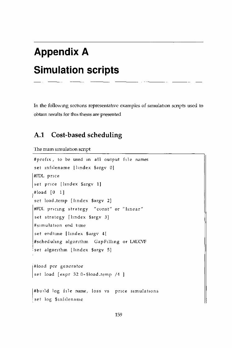
Appendix A
Simulation scripts
In the following sections representative examples of simulation scripts used to
obtain results for this thesis are presented
A.l Cost-based scheduling
The main simulation script
#pre f ix , to be used in a l l ou tpu t f i l e names
set m f i l e na m e [ l m d e x $argv 0]
#FDL pr ice
set p r i ce [ l m d e x $argv 1]
#load [0 1]
set load^temp [ l m d e x $argv 2]
#FDL p r i c i ng s t r a t e g y " co ns t " or " l i n e a r "
set s t r a t e g y [ l m d e x $argv 3]
#s i mu la t i on end t ime
set endt ime [ l m d e x $argv 4]
#s chedu l ing a lgor i t hm Ga pF i l l mg or LAUCVF
set a lgor i t hm [ l i ndex $argv 5]
#load per g en e r a t o r
set load [expr 32 0 * $load_temp /4 ]
#bu i l d log f i l e name, loss vs p r i ce s imu la t i on s
set log $ inf i l enamc
159
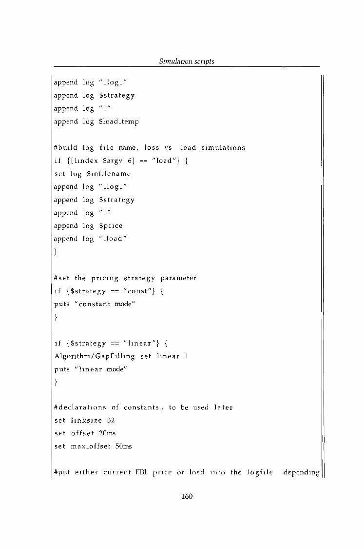
Simulation scripts
append log "_log_"
append log $ s t r a t eg y
append log
append log $load_temp
#bui ld log f i l e name, loss vs load s imu l a t i o ns
if { [ l i ndex $argv 6] == " load"} {
set log $ mf i l en ame
append log "_log_"
append log $ s t r a t eg y
append log
append log $pr ice
append log "_ load"
}
# s e t the p r i c in g s t r a t e g y parameter
if { $s t r a t eg y == "cons t "} {
put s " c o n s t a n t mode"
}
if { $ s t r a t e gy == " l i n e a r " } {
A l g o r i t hm / G ap F i l h n g set l i n e a r 1
puts " l i n e a r mode"
}
# d e c l a r a t i o n s of cons t an t s , to be used l a t e r
se t l i n k s i z e 32
set o f f s e t 20ms
set max-of f se t 50ms
#put e i t h e r c u r r e n t FDL pr i ce or load in to the l og f i l e depending
160
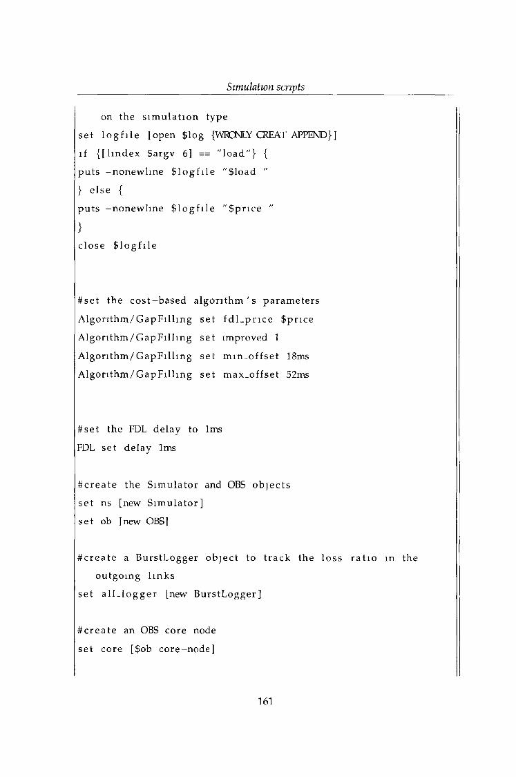
Simulation scripts
on the s i mu l a t i o n type
set l o g f i l e [open $log {VVFOsLY CREAT APPEND}]
if { [ l i ndex $argv 6] == " load"} {
puts —nonewline $ l o g f i l e "$load "
} e l se {
puts -nonewl ine $ l o g f i l e "$p r i ce "
}
close $ l o g f i l e
#se t the c os t - b a s e d a l g o r i t h m ' s paramete r s
A l g o r i t h m / Ga pF i l l m g set f d l . p r i c e $pr ice
A l g o n t h m / G a p F i l l i n g set improved 1
A l g o r i t h m / Ga pF i l l m g set mm _ o f f se t 18ms
A l g o r i t h m / Ga pF i l l mg set max . of f s e t 52ms
#se t the FDL delay to 1ms
FDL set delay 1ms
# c r e a t e the Simula tor and OBS ob jec t s
se t ns [new Simula to r ]
se t ob [new OBS]
# c r e a t e a Burs tLogger ob j ec t to t r ack the loss r a t i o m the
outgoing l i nks
set a l l - l o g g e r [new Burs tLogger]
# c r e a t e an OBS core node
set core [$ob core-node]
161
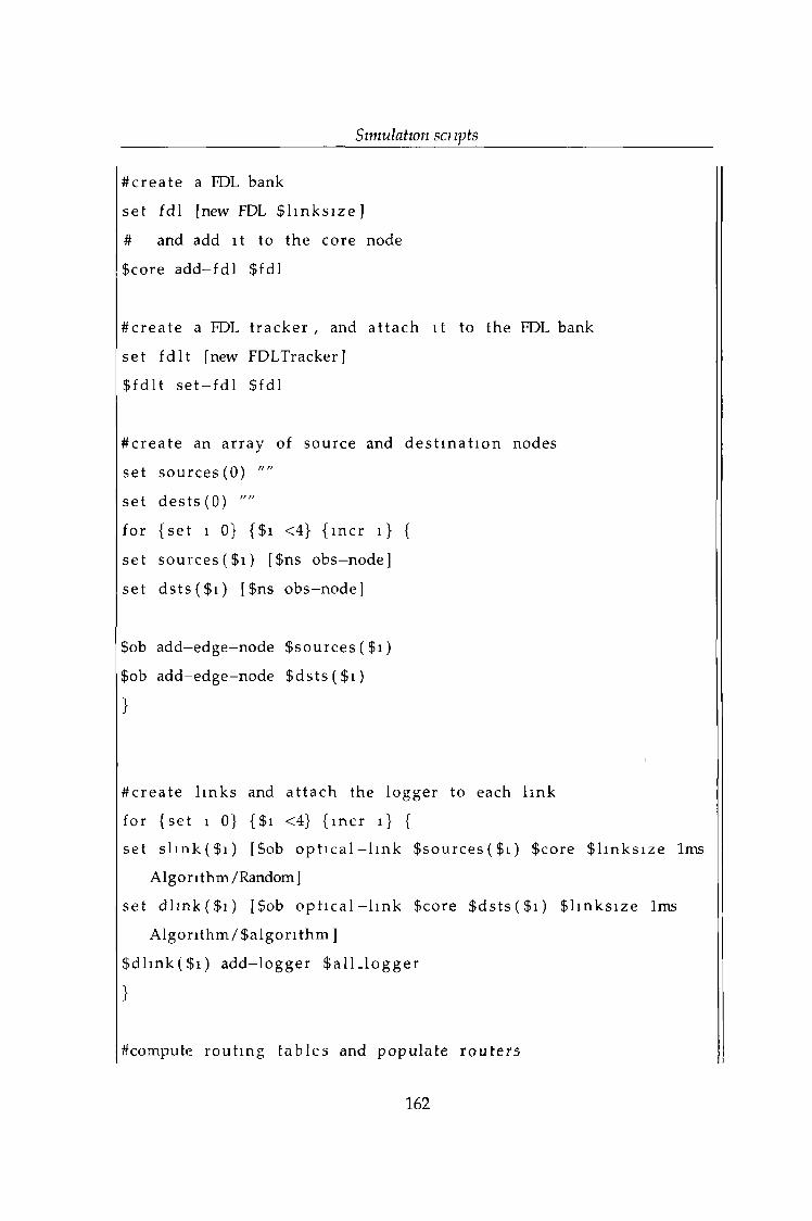
Simulation sci ipts
# c r e a t e a FDL bank
se t fdl [new FDL $ h n k s i z e ]
# and add i t to the core node
Score a d d - f d l $f d 1
# c r e a t e a FDL t r acke r , and a t t a c h i t to the FDL bank
set f d l t [new FDLTracker]
$ f d 11 s e t - f d l $f d 1
# c r ea t e an a r ray of source and d e s t i n a t i o n nodes
set s o u r c e s (0) ""
set des t s (O) ""
for {se t i 0} {$i <4} { inc r i } {
se t s o u r c e s ( $ i ) [$ns obs—node]
set d s t s ( $ i ) [$ns obs-node]
$ob add-edge-node $ s o u r c e s ( $ i )
$ob add-edge-node $ d s t s ( $ i )
}
1
# cr e a t e l i nks and a t t a c h the logger to each l ink
for {set i 0} {$i <4} { incr 1 } {
set s l m k ( $ i ) [$ob o p t i c a l —l ink $ s o u r c e s ( $ i ) Score $ l i n k s i z e 1ms
Algori thm/Random]
se t d h n k ( $ i ) [$ob o p t i c a l —l ink Score $ d s t s ( $ i ) S l i nk s i z e 1ms
A l g o n t h m / S a l g o n t h m ]
Sdl ink ( $ i ) a dd- l ogge r $ a l l _ l og ge r
}
^compute rou t i ng t a b l e s and popu la t e r o u t e r s
162
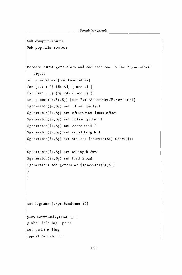
Simulation scripts
Sob compute—rou tes
$ob popula te —r o u t e r s
# c r e a t e b u r s t ge ne r a t o r s and add each one to the " g e n e ra t o r s
ob j ec t
set ge ne r a t o r s [new Genera tor s ]
for {se t 1 0} { $ 1 <4} { incr 1 } {
for {se t j 0} {$j <4} { incr j} {
set g ene r a t o r ( $i , $ j ) [new Bur s tAssembler /Exponen t i a l ]
Sgenera tor ( $i , $ j ) se t o f f s e t $ o f f se t
Sgenera tor ( $i , $ j ) se t o f f se t . max $max_offset
$gener a to r ( $i , $ j ) set o f f s e t - j i t t e r 1
$ g e n e r a t o r ( $i , $ j ) se t c o r r e l a t e d 0
$gene r a t o r ( $i , $j ) se t c ons t _ l eng t h 1
$gene r a t o r ( $i , $ j ) s e t - s r c - d s t $ s ou r c e s ( $ i ) $ d s t s ( $ j )
$gener a to r ( $i , $ j ) se t av length 3ms
$gener a to r ( $i , $ j ) set load $load
$gene r a t o r s a d d - g e n e r a t o r $gene r a t o r ( $ i , $ j )
}
}
set logt ime [expr $endt ime +1]
proc s ave -h i s tog r a ms {} {
g loba l f d l t log pr i ce
se t o u t f i l e $log
append o u t f i l e
163
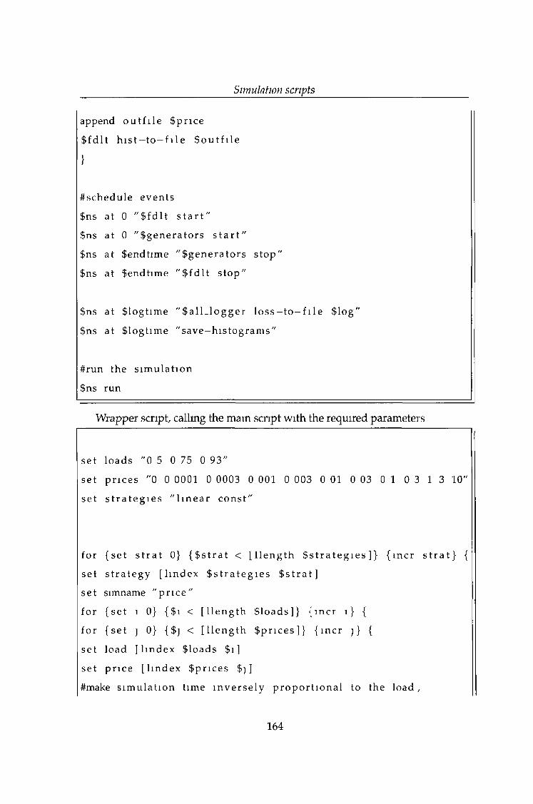
Simulation scripts
append o u t f i l e $pr i ce
$ fd 11 h i s t —t o—f i l e $ o u t f i l e
}
#schedule events
$ns at 0 " $ f d l t s t a r t "
$ns at 0 " Sgene ra tor s s t a r t "
$ns at $endt ime " $ g e n e r a t o r s s top"
$ns at $endt ime " $ f d l t s top"
$ns at $logt ime " $ a l l _ l o g g e r l o s s - t o - f i l e $log"
$ns at $logt ime " save—his tograms"
#run the s i mu l a t i on
$ns run
Wrapper script, calling the main script with the required parameters
set loads "0 5 0 75 0 93"
set pr i ce s "0 0 0001 0 0003 0 001 0 003 0 01 0 03 0 1 0 3 1 3 10"
set s t r a t e g i e s " l i n e a r cons t "
for {se t s t r a t 0} { $ s t r a t < [ l l e n g t h $ s t r a t e g i e s ]} { incr s t r a t } {
set s t r a t e g y [ l index $ s t r a t e g i e s $ s t r a t ]
set simname " p r i c e "
for {se t i 0} {$i < [ l l e n g t h $loads]} { incr 1 } {
for {se t ] 0} {$] < [ l l e n g t h $ pr i c e s ] } { incr j } {set load [ l i ndex $loads $i ]
set p r i ce [ l i ndex $pr i ces $) ]
#make s imu l a t i on t ime i n v e r s e l y p r o p o r t i o n a l to the load ,
164
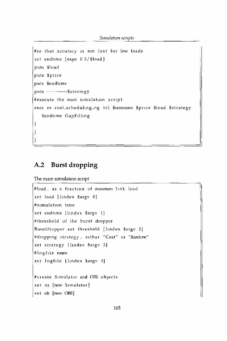
Simulation scripts
#so t ha t accuracy is not l o s t for low loads
set endt ime [expr 0 3 / $ l o a d ]
puts $load
puts $pr ice
put s $endt ime
puts -------------- $ s t r a t eg y
#execute the main s imu l a t i on s c r i p t
exec ns c os t _ s chedu l mg_ng t e l $simname $pr ice $load $ s t r a t eg y
$endt ime G a p F i l h n g
}
}
}
A.2 Burst dropping
The main simulation script
#load , as a f r a c t i o n of maximum l ink load
set load [ l i ndex $argv 0]
# s i mu la t i o n time
set endt ime [ l i ndex $argv 1]
# t h r e s h o l d of the b u r s t dropper
Burs tDropper set t h r e sh o l d [ l i ndex $argv 2]
#droppmg s t r a t e g y , e i t h e r "Cost" or "Random"
set s t r a t e g y [ l index $argv 3]
# 1 o g f 1 1 e name
set l o g f i l e [ l i ndex $argv 4]
# c r e a t e Simula tor and OBS ob jec t s
se t ns [new Simula tor ]
se t ob [new OBS]
165
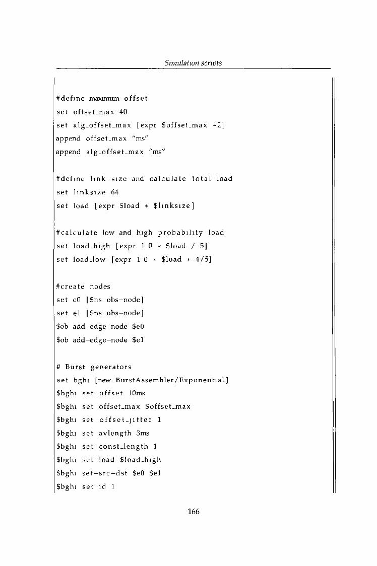
Simulation scripts
# d e f m e maximum o f f s e t
set o f f se t . max 40
set a lg_of fse t_max [expr $offset_max +2]
append o f f se t . max "ms"
append a lg_of fse t_max "ms"
# d e f m e l ink s ize and c a l c u l a t e t o t a l load
set h n k s i z e 64
set load [expr $load * $ h n k s i z e ]
# c a l c u l a t e low and high p r o b a b i l i t y load
set l o a d . h i gh [expr 1 0 * $load / 5]
se t load- low [expr 1 0 * $load * 4 /5]
# c r e a t e nodes
set eO [$ns obs-node]
set el [$ns obs-node]
$ob add-edge—node $e0
$ob add-edge-node $el
# Burst ge ne r a t o r s
set bghi [new Burs tAssembler / Exponent i a l ]
$bghi set o f f s e t 10ms
$bghi set o f f se t . max $offset_max
$bghi set of f se t _j i t t e r 1
$bghi set av l eng t h 3ms
$bghi set cons t _ l eng t h 1
$bghi set load $load_high
$bghi s e t - s r c —dst $e0 $el
$bghi set id 1
166

Simulation scripts
# low p r i o r i t y g e ne r a t o r
set bglo [new Bur s t Assembl e r / Exponen t i a l ]
$bglo set o f f s e t 10ms
$bglo set o f f se t . max $offset_max
$bglo set o f f s e t - ] i t t e r 1
$bglo set av l eng t h 3ms
$bglo set c ons t _ l eng t h 1
$bglo set load $load_low
$bglo s e t — s r c — dst $e0 $el
$bglo set id 2
#add ge ne r a t o r s to a " Gene r a t o r s " object , for e a s i e r management
set ge ne r a t o r s [new Genera to r s ]
$gene r a t o r s add—g e ne r a t o r $bghi
$ gene r a t o r s add—g e ne r a t o r $bglo
#c onf i gure the c os t - b a s e d a lgor i thm
A l g o r i t hm / G ap F i l h n g set l eve l 30
A l g o n t h m / G a p F i l h n g set m m . o f f s e t 9ms
Algo r i t hm/ GapF i l l i ng set max . o f f s e t $a lg_of fse t_max
A l g o r i t h m / Ga pF i lh n g set debug 0
# impor t an t — t ry to make the cost func t i on i ndependent on the
o f f s e t t ime
A l g o r i t hm / G ap F i l h n g set improved 1
# c r e a t e l ink
set l i nk [$ob o p t i c a l - h n k $e0 $el $ l i n k s i z e 1ms "Algor i thm/
GapFi l l i ng "]
# c r e a t e and conf igure dropper
set dropper [new B ur s t D r o p p e r / $ s t r a t e gy ]
167
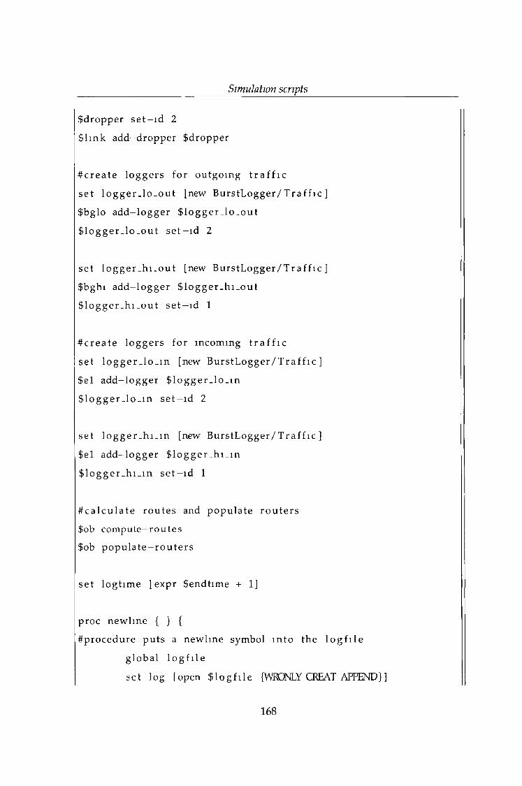
Simulation scripts
$dropper s e t - i d 2
$l ink add-dropper $dropper
# c r ea t e loggers for outgoing t r a f f i c
set logge r_ lo_ou t [new B u r s tL o g g e r / T r a f f i c ]
$bglo a dd - l ogge r $ l o g g e r . l o g o u t
$ logger_ lo_out s e t - i d 2
set l ogge r_h i_ou t [new Bu r s t Lo g ge r / T r a f f i c ]
$bghi add—logger $ l ogge r_h i_out
$ logger_h i_out s e t —id 1
# c r e a t e loggers for incoming t r a f f i c
set l o g g e r _ l o _ m [new B u rs t L o g g e r / T r a f f i c ]
$el a dd - l ogge r $ logger_ lo_ in
$ l o g ge r_ lo _m s e t —id 2
set l ogge r_h i_ in [new B u r s t L o g g e r / T r a f f i c ]
$el a dd- l ogge r $ logge r_h i_ in
$ l o g ge r_ h i _m s e t - i d 1
# c a l c u l a t e rou t e s and popula t e r o u t e r s
$ob compute—rou tes
$ob popula te —r o u t e r s
set logt ime [expr $endt ime + 1]
proc newl ine { } {
#procedure put s a newl ine symbol in to the l o g f i l e
g loba l l o g f i l e
set log [open $ l o g f i l e {WKQNLY CREAT APPEND}]
168
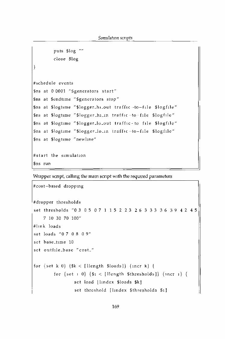
Simulation scripts
puts $log ""
c lose $log
}
#schedule events
$ns at 0 0001 " { g e n e r a t o r s s t a r t "
$ns at $endt ime " $ gene r a t o r s s top"
$ns at $logt ime " $ l ogge r _h i _ou t t r a f f i c —to —f i l e $ l o g f i l e "
$ns at $logt ime " $ l og ge r_ h i _m t r a f f i c —to —f i l e $ l o g f i l e "
$ns at $logt ime " S logger _lo_out t r a f f i c —t o—f i l e $ l o g f i l e "
$ns at $logt ime " $ l og ge r_ l o_ m t r a f f i c —to—f i l e $ l o g f i l e "
$ns at $logt ime "newl ine"
# s t a r t the s i mu l a t i on
$ns run
Wrapper script, calling the main script with the required parameters
# co s t—based dropping
#dropper t h r e s h o l d s
set t h r e s h o l d s "0 3 0 5 0 7 1 1 5 2 2 3 2 6 3 3 3 3 6 3 9 4 2 4 5
7 10 30 70 100"
# h n k loads
set loads "0 7 0 8 0 9"
set base_t ime 10
set o u t f i l e . b a s e " co s t_ "
for {se t k 0} {$k < [ l l e n g t h $ loads]} { incr k} {
for {se t i 0} {$i < [ l l e n g t h { t h r e sh o ld s ]} { incr 1 } {
set load [ l i nd ex $loads $k]
set t h r e sho l d [ l i ndex { t h r e sh o ld s Si ]
169
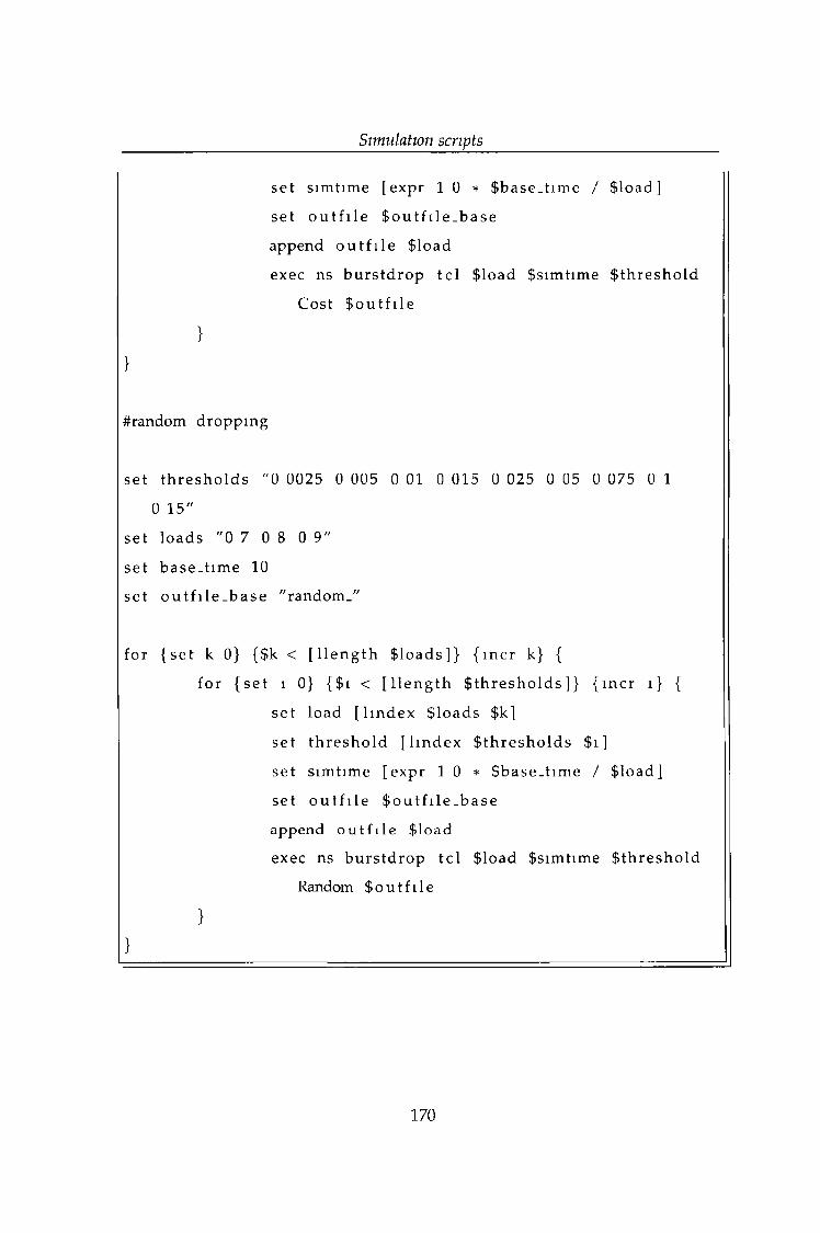
Simulation scripts
set s imtime [expr 1 0 * $base_t ime / $load]
set o u t f i l e $ o u t f i l e _b a s e
append o u t f i l e $load
exec ns bu r s t d r op te l $load $simtime $ th resho ld
Cost $ o u t f i l e
}
}
#random dropping
set t h r e s h o l d s "0 0025 0 005 0 01 0 015 0 025 0 05 0 075 0 1
0 1 5 "
set loads "0 7 0 8 0 9"
set base - t ime 10
set o u t f i l e - b a s e "random."
for {se t k 0} {$k < [ l l e n g t h $loads]} { incr k} {
for {se t i 0} {$i < [ l l e n g t h $ t h re sh o l ds ]} { incr 1 } {
set load [ l m d e x $loads $k]
set t h re sh o l d [ l i ndex $ t h r e s h o l ds $i]
se t s imtime [expr 1 0 * $base_t ime / $load]
set o u t f i l e $ o u t f i l e _b a s e
append o u t f i l e $load
exec ns bu r s t d r op t e l $load $simtime $ th r e s ho l d
Random $ o u t f i l e
}
}
170
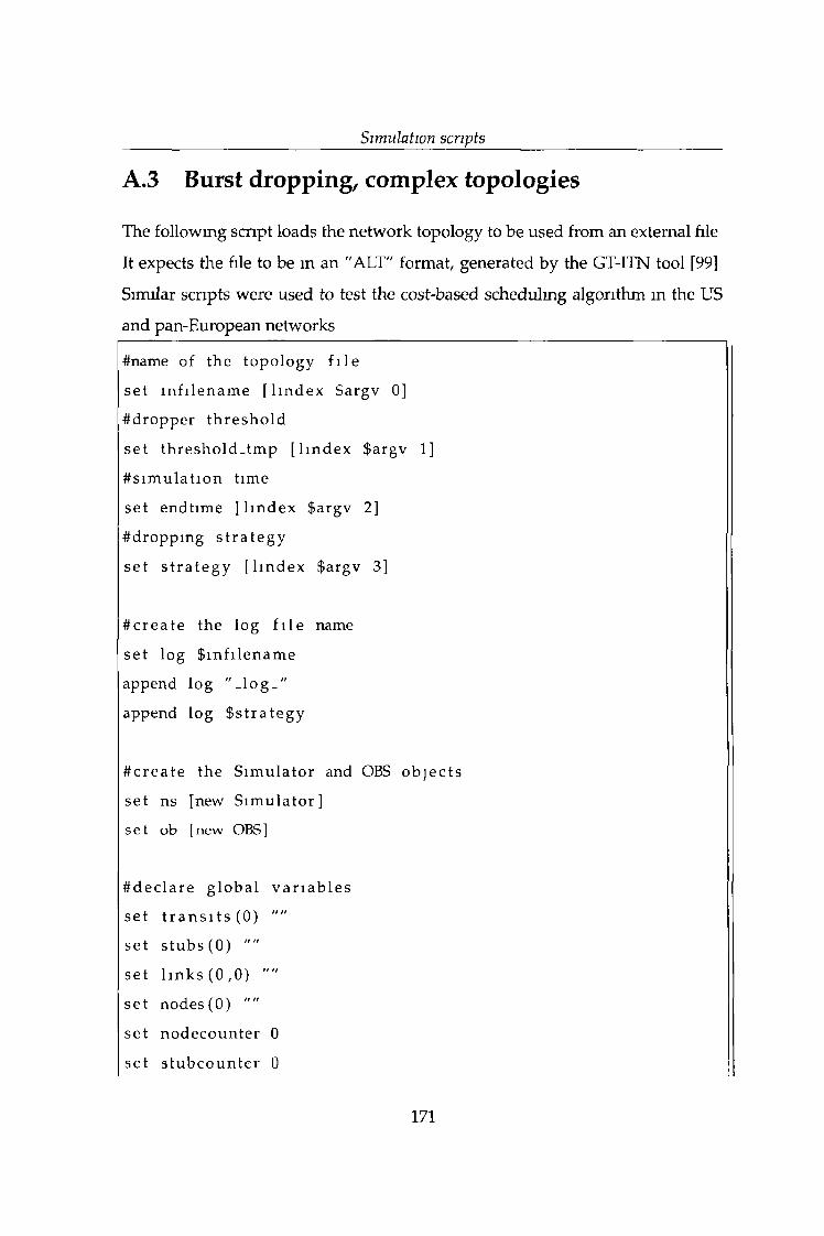
Simulation scripts
A.3 Burst dropping, complex topologies
The following script loads the network topology to be used from an external file
It expects the file to be in an "ALT" format, generated by the GT-ITN tool [99]
Similar scripts were used to test the cost-based scheduling algorithm in the US
and pan-European networks
#name of the topology f i l e
se t i n f i l ename [ l i ndex $argv 0]
#dropper t h r e sho l d
set t h r e sh o l d . t mp [ l i ndex $argv 1]
# s i mu la t i o n t ime
set endt ime [ l i ndex $argv 2]
#dr oppmg s t r a t e g y
set s t r a t e g y [ l i ndex $argv 3]
# c r e a t e the log f i l e name
set log $ mf i l ena me
append log "_log_"
append log $ s t r a t eg y
# c r ea t e the Simula tor and OBS objec t s
set ns [new Simula tor ]
set ob [new OBS]
#d ec l a r e g loba l v a r i a b l e s
set t r a n s i t s (0) ""
set s t u b s (0) ""
set l i nks (0 ,0 ) ""
set n o d es (0) ""
set nodecounter 0
set s t ub co u n t e r 0
171
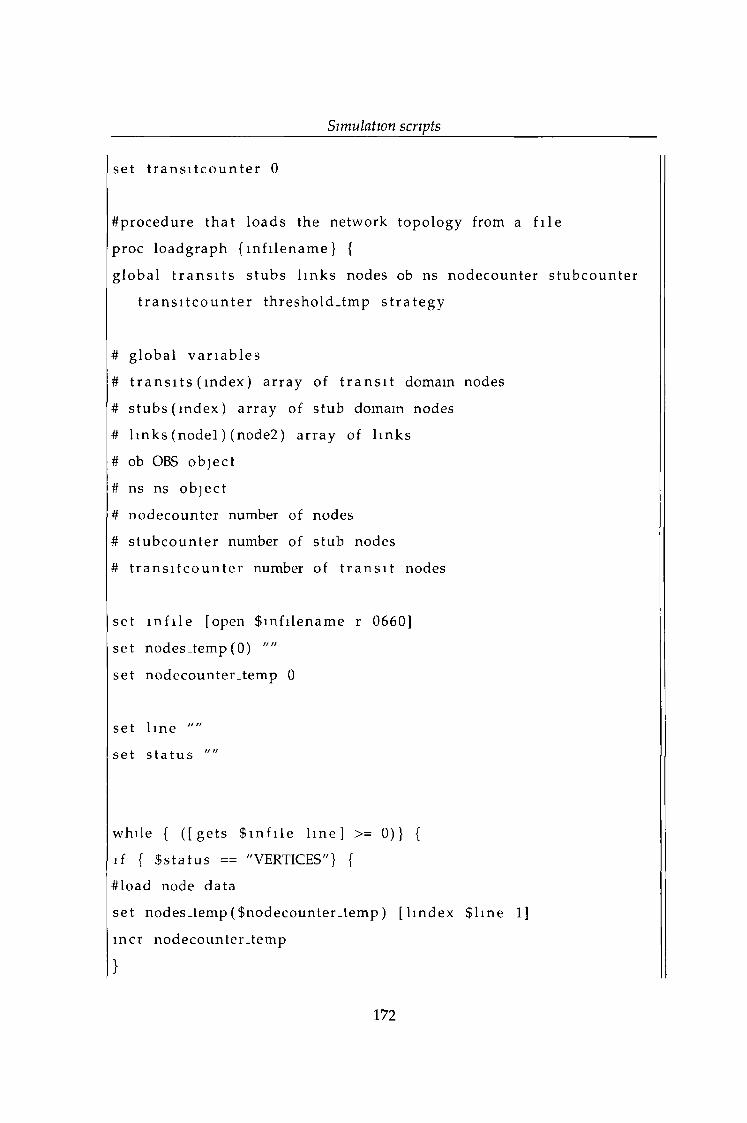
Simulation scripts
set t r a n s i t c o u n t e r 0
#procedure t ha t loads the network topology from a f i l e
proc l oadgraph { mf i l e na me } {
globa l t r a n s i t s s tubs l i nks nodes ob ns nodecounter s t ubcoun t e r
t r a n s i t c o u n t e r t h r e s ho ld . t m p s t r a t e g y
# globa l v a r i a b l e s
# t r a n s i t s ( i n d e x ) a r ray of t r a n s i t domain nodes
# s tubs ( index) a r ray of s tub domain nodes
# l i nks ( n o d e l ) (node2) a r ray of l i nks
# ob OBS object
# ns ns objec t
# nodecounter number of nodes
# s t ub co un t e r number of s tub nodes
# t r a n s i t c o u n t e r number of t r a n s i t nodes
set i n f i l e [open $ mf i l en a me r 0660]
set nodes_temp (0) ""
set nodecounter_temp 0
set l ine ""
set s t a t u s ""
whi le { ( [ g e t s $ m f i l e l i n e ] >= 0)} {
if { $ s t a t u s == "V E R T IC E S"} {
#load node data
set nodes_temp ( $nodecounter_temp ) [ l i ndex $ h n e 1]incr nodecounter_temp
}
172
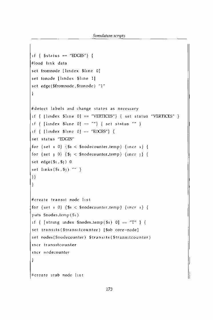
Simulation scripts
if { Ss t a tus == "EDGES"} {
#load l ink data
set fromnode [ h n d e x $ h n e 0]
set tonode [ h n d e x $ h n e 1]
set edge ( $fromnode, $ t onode ) "1"
}
# d e t e c t l a be l s and change s t a t e s as necessa ry
if { [ h n d e x $ h n e 0] == "VERTICES"} { set s t a t u s "VERTICES" }
if { [ h n d e x $ h n e 0] == ""} { se t s t a t u s "" }
if { [ h n d e x $ h n e 0] == "EDGES"} {
set s t a t u s "EDGES"
for {se t i 0} {$i < $nodecounter_temp} { incr 1 } {
for {se t ] 0} {$] < $nodecounter_temp} { incr j} {
set edge ( $i , $ j ) 0
set l i nks ( $i , $]) "" }
}}
}
# c r e a t e t r a n s i t node l i s t
for {set i 0} {$i < $nodecounter_temp} { m c r 1 } {
puts $nodes_temp ( $ i )
if { [ s t r i n g index $nodes_temp ( $ i ) 0] == "T" } {
set t r a n s i t s ( $ t r a n s i t c o u n t e r ) [$ob core—node]
set n od es ( $ nodecoun t e r ) $ t r a n s i t s ( $ t r a n s i t c o u n t e r )
incr t r a n s i t c o u n t e r
incr nodecounter
}
# crea t e s tub node l i s t
173
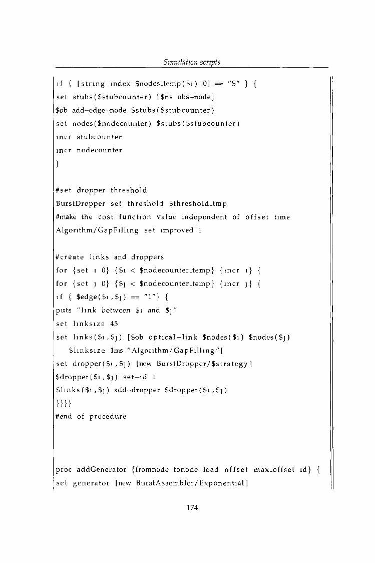
Simulation scripts
if { [ s t r i n g index $nodes_temp ( $ 1 ) 0] == "S" } {
set s tubs ( $s t ubcoun t e r ) [$ns obs-node]
$ob add-edge-node $ s t u b s ( $ s t u b c o u n t e r )
se t nodes ( $ nodecoun t e r ) $ s tubs ( $ s tub coun te r )
i ncr s tu bco un t e r
incr nodecounter
}
#se t dropper t h r e s ho l d
Burs tDropper set t h r e s h o l d $threshold_tmp
#make the cost func t i on value independent of o f f s e t t ime
A l g o r i t h m / G ap F i l h n g set improved 1
#c r ea t e l i nks and droppers
for {se t 1 0} {$i < $nodecounter_ temp} { incr 1 } {
for {set j 0} {$) < $nodecounter_temp} { incr j} {
if { $ e d g e ( $ i , $ j ) = "1"} {puts " l i n k between $i and $ j "
set h n k s i z e 45
set h n k s ( $ i , $ j ) [$ob o p t i c a l —l ink $nodes ( $ i ) $nodes ( $ j )
$ h n k s i z e 1ms " A l g o n t h m / G a p F i l l m g "]
set dropper ( $i , $)) [new B u r s t D r o p p e r / $ s t r a t e g y ]
$dropper ( $ i , $]) s e t - i d 1
$ l inks ( $i , $]) add-dropper $dropper ( $i , $ j )
} } }}
#end of procedure
proc addGenerator {fromnode tonode load o f f s e t max .of f se t id} {
set g en er a t o r [new Burs t Assembl e r / Exponen t i a l ]
174
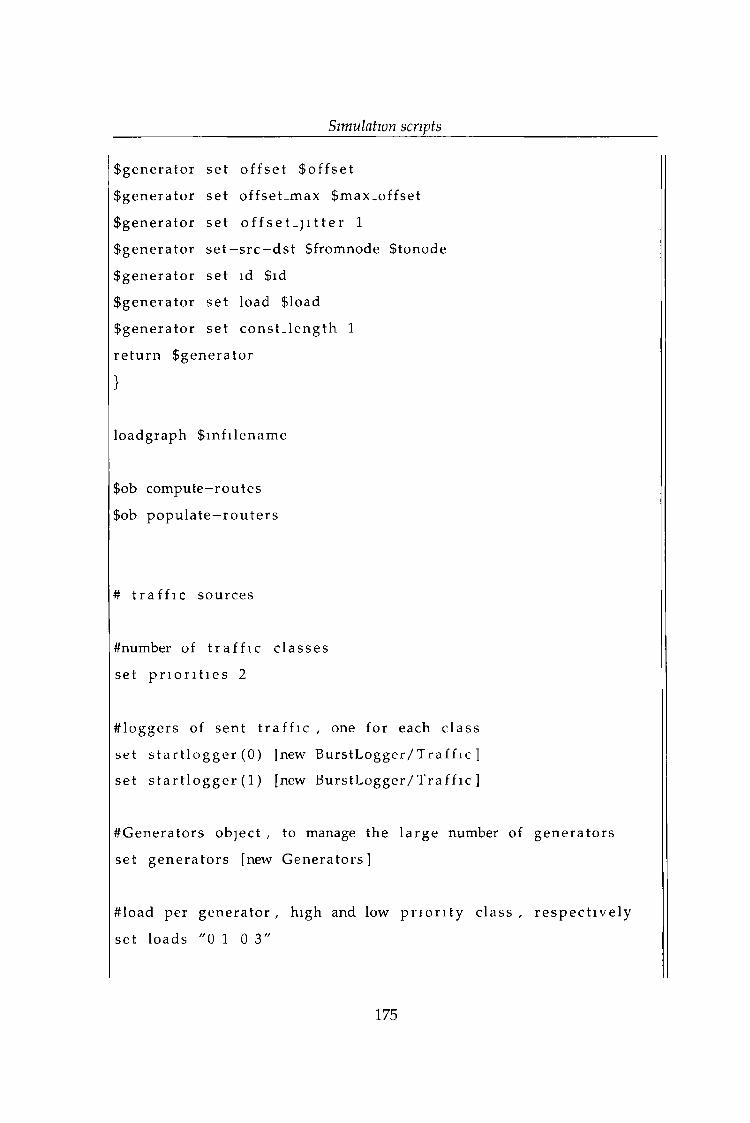
Simulation scripts
$gener a to r set o f f s e t $ o f f se t
$gener a to r set offset_max $max_offset
$gener a to r set of f se t - j 1 1 te r 1
$gener a to r s e t - s r c - d s t $fromnode $tonode
$gene r a t o r set id $id
$gene r a t o r s e t load $load
$gener a to r set c o n s t . l e n g t h 1
r e t u r n $gener a to r
}
loadgraph $ mf i l ena me
$ob compute - routes
$ob p o p u l a t e - r o u t e r s
# t r a f f i c sources
#number of t r a f f i c c l a s ses
set p r i o r i t i e s 2
# logge r s of sent t r a f f i c , one for each c l as s
set s t a r t l o g g e r (0) [new B u r s tL o g g e r /T r a f f i c ]
se t s t a r t l o g g e r (1) [new Bu r s t Lo g g e r / T r a f f i c ]
#Genera to r s object , to manage the l a rge number of
set ge ne r a t o r s [new Genera tor s ]
#load per genera tor , high and low p r i o r i t y c lass ,
se t loads "0 1 0 3"
ge ne r a t o r s
r e s p e c t i v e l y
175
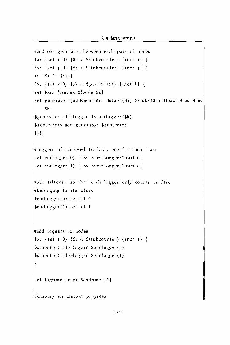
Simulation scripts
#add one gene r a t o r between each pa i r of nodes
for {set 1 0} { $ 1 < $ s t u b c o u n t e r } { incr 1 } {
for {se t j 0} {$] < $ s t u b c o u n t e r } { incr j } {
i f {$i »= $)} {
for {se t k 0} {$k < $ p r i o r i t i e s } { incr k} {
set load [ h n d e x $loads $k]
set g ene r a t o r [ addGenerator $ s t u b s ( $ i ) $ s t u b s ( $ j ) $load 30ms 50ms
$ k ]
$ gener a t o r add—logger $ s t a r t l o g g e r ( $k)
$ gene r a t o r s a d d - g e n e r a t o r Sgenera tor
} } }}
# logger s of rece ived t r a f f i c , one for each c l as s
set endlogger(O) [new B u r s t L o g g e r / T r a f f i c ]
se t e n d l o g g e r ( l ) [new B u r s t L o g g e r / T r a f f i c ]
# s e t f i l t e r s , so t h a t each logger only counts t r a f f i c
#be l ongmg to i t s c l ass
Sendlogger (0) s e t —id 0
$ en d l og ge r (1) s e t - i d 1
#add loggers to nodes
for {se t i 0} {$i < $ s t u b c o u n t e r } { incr 1 } {
$ s t u b s ( $ i ) ad d - l og ge r $ e n d l og g e r (0)
$ s t u b s ( $ i ) add—logger $ e n d l og g e r (1)
}
set logt ime [expr $endt ime +1]
# d i s p l a y s imu l a t i on p rogr es s
176
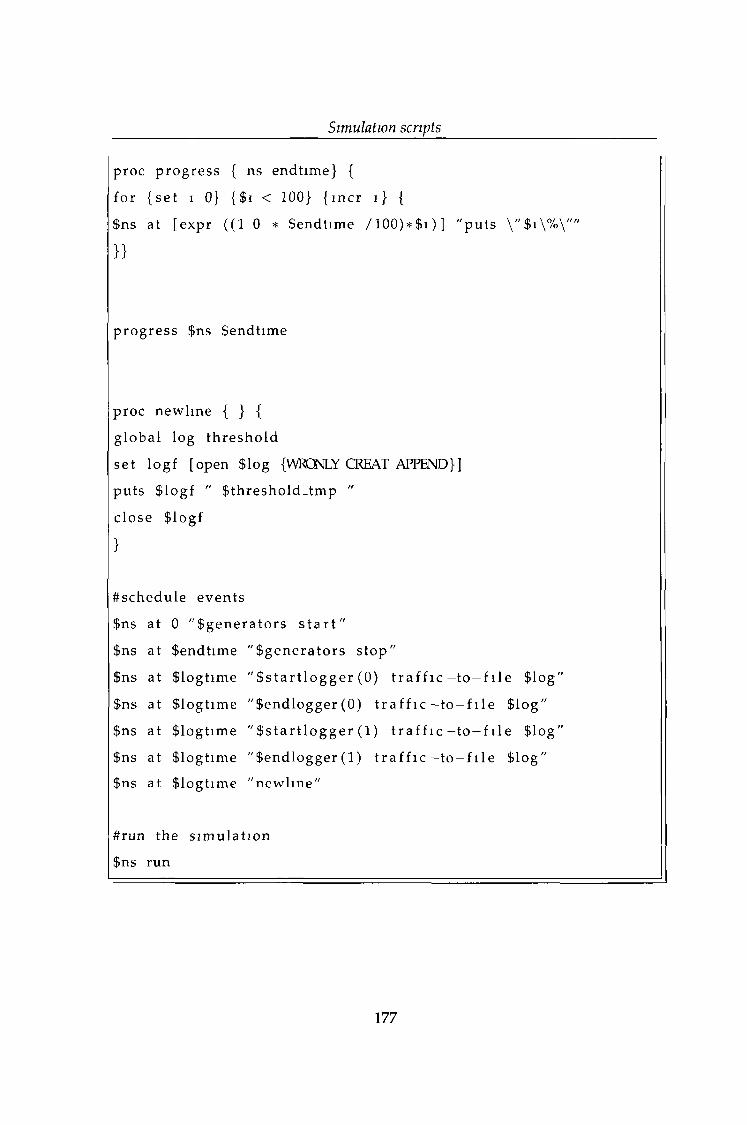
Simulation scripts
proc progress { ns endtime} {
for {set 1 0 } {$i < 100} {incr 1} {
$ns at [expr ( (1 0 * $endtime / 100)*$ i)] "puts
}}
progress $ns $endtime
proc newlme { } {
global log th resho ld
set logf [open $log {WKONLY CREAT APPEND}]
puts $logf " $threshold_tmp "
close $logf
}
#schedule events
$ns at 0 "$genera to rs s t a r t "
$ns at $endtime "$genera to rs stop"
$ns at $logtime " $ s ta r t lo g g e r (0 ) t r a f f i c - t o - f i l
$ns at $logtime "$endlogger (0 ) t r a f f i c —to—fi le
$ns at $logtime " $s t a r t l ogge r ( 1 ) t r a f f i c - t o - f i l
$ns at $logtime "$endlogger (1 ) t r a f f i c —to —fi le
$ns at $logtime "newlme"
#run the s im ulation
$ns run
e $log"
$log"
e Slog"
$log"
177