cost economies and market power in u.s. beef packingcost economies and market power. the...

Cost Economies and Market Powerin U.S. Beef Packing

Catherine J. Morrison Paul

Giannini Foundation Monograph Number 44

May 2000

DIVISION OF AGRICULTURE AND NATURAL RESOURCESCALIFORNIA AGRICULTURE EXPERIMENT STATION

OAKLAND, CALIFORNIA

Giannini Monograph Number 44 i

CONTENTS

CONTENTS

1 INTRODUCTION 1

2 OVERVIEW OF METHODOLOGICAL ISSUES 3

3 THE PRODUCTION STRUCTURE MODEL IN MORE DETAIL 7

4 EMPIRICAL IMPLEMENTATION OF THE MODEL 11

5 INDICATORS CONSTRUCTED FROM THE ESTIMATED MODEL 155.1 Cost Economy Measures . . . . . . . . . . . . . . . . . . . . . . . . . . . 155.2 Market Power Measures. . . . . . . . . . . . . . . . . . . . . . . . . . . . 18

6 FURTHER MEASUREMENT AND INTERPRETATION ISSUES 216.1 Linkages among cost economy and market power measures . . . . . . . . . 216.2 Sub- and combination-production structure measures . . . . . . . . . . . . 236.3 Additional cost and market structure measures . . . . . . . . . . . . . . . . 25

7 THE EMPIRICAL RESULTS 27

8 CONCLUDING REMARKS 33

TABLE S1 – SUMMARY STATISTICS 35

REFERENCES 37

A SUMMARY OF VARIABLES, MEASURES, TERMS AND EQUATIONSVariable definitions . . . . . . . . . . . . . . . . . . . . . . . . . . . . . . . . . 39Overview of constructed measures . . . . . . . . . . . . . . . . . . . . . . . . . 40

B DATA TABLES – VALUE, QUANTITY, PRICE AND RATIO MEASURESTable B1 – Categories and regions . . . . . . . . . . . . . . . . . . . . . . . . . 44

C ADDITIONAL MEASURES FOR CATEGORIES AND REGIONSTable C1 – Coefficient estimates . . . . . . . . . . . . . . . . . . . . . . . . . . 50Table C2 – Scale economies and price ratios . . . . . . . . . . . . . . . . . . . . 52Table C3 – Scope and labor demand elasticities . . . . . . . . . . . . . . . . . . 54Table C4 – Energy demand and shadow value elasticities . . . . . . . . . . . . . 56Table C5 – Input supply and cost economy elasticities. . . . . . . . . . . . . . . 58Table C6 – Markdown and markup elasticities . . . . . . . . . . . . . . . . . . . 60

D DATA SUPPLEMENT 62

Giannini Monograph Number 44 1

1. INTRODUCTION

Concerns about market power in the beef packing industry, and its impact on bothproducers of farm inputs (cattle) and consumers of beef products, have been raised in theUnited States for more than a century. As highlighted by Azzam and Schroeter [1997],in 1888, the US Senate adopted a resolution to “examine fully all the questions touchingthe meat products of the United States,” and especially to investigate whether “thereexists or has existed any combination of any kind…by reason of which the prices of beefand beef cattle have been so controlled or affected as to diminish the price paid theproducer without lessening the cost of meat to the consumer.” In the 1990s, theseconcerns have again come to the forefront due to dramatic increases in concentration inthis industry since the late 1970s.

Concentration levels dropped from their peak in 1888 when the “Big Fourslaughtered 89 percent of the cattle in Chicago and produced two-thirds of the country’sdressed beef supply,” to a low in 1977 “with 22 percent of cattle slaughter and 20 percentof fed steer and heifer slaughter controlled by the four largest packers” (Azzam andSchroeter, p. 26). Then, with the advent of new production processes, concentrationlevels again began to escalate. In particular, more fabrication was evident with a movetoward “boxed beef” production (individually packaged cuts rather than carcasses as theprimary output). Low capacity utilization levels also prevailed, due to falling demand forred meat products. These and other factors resulted in a wave of consolidation, where theshare of the top four packers rose to 82 percent in 1994.

The resulting perception, as in the late 1800s, is that this has reduced the welfare ofthe agricultural community through lower cattle prices to farmers than would have existedin a competitive environment. Some have also blamed the apparent lack of competitionin this industry for higher consumer prices for beef products than can be attributed just tothe strength of meat demand.

These concerns raised by observed market structure trends are based on the specter ofan “abuse of market power” in both output and input markets, including the potential forexcess markups of output prices and markdowns of input prices from those that wouldprevail under more competitive conditions. Allegations of lack of competition and abuseof market power have, however, been tempered somewhat by the recognition thatconsolidation could have potentially been caused by efficiency gains, supporting lowercost production and greater productivity than otherwise would be possible.

That is, the technological base could be such that cost efficiencies are captured bylarge producers (plants and firms) if cost economies exist in the industry. Sucheconomies could include utilization (short run), scale (long run), or size (differential inputcomposition) economies, scope economies, and multiplant economies. If these types ofcost economies are evident, lower costs allowed by large-scale, diversified, and jointoperations could potentially be passed on in the form of better market conditions for bothconsumers of final products and producers of primary inputs (cattle).

If such efficiencies or economies exist, however, the usual “test” for market powerbased on the deviation between price and marginal cost (for an output, or similarly theprice and shadow value for an input) may be misleading. Specifically, the impacts of costeconomies on the gap between marginal and average costs are important to recognize andmeasure for appropriate evaluation and interpretation of production (technological andmarket) structure, and its implications for consumer and farmer welfare.

Characterization of the cost structure is therefore a crucial part of the puzzle whenevaluating “the questions touching the meat products of the United States” (as stated inthe 1888 US Senate resolution) – especially, the causes and welfare consequences ofconcentration or market power. To pursue this characterization, in this study we haveused cost and revenue data from a USDA/GIPSA (Grain Inspection, Packers andStockyards Administration) survey of US beef packing plants to carry out a detailedanalysis of the production structure of these plants, with a particular focus on measures ofcost economies and market power.

The methodological approach is based on a cost function model of plants in thisindustry, with profit maximization over cattle purchases, and fabricated (boxed beef),slaughter (carcasses), hide, and byproduct output production incorporated. Various

2 Morrison Paul

technological and market structure characteristics have been recognized in the model toallow their impacts to be estimated. Cost economies from short-run, long-run, andinput-biased scale economies, as well as jointness deriving from output diversification(scope economies) and spillovers across plants (multiplant economies) are accommodatedand measured. Market power parameters for (fabricated) outputs and cattle inputs areestimated to facilitate evaluation of output price markups and input (cattle) pricemarkdowns due to monopoly and monopsony power. A cattle-price relationship isincluded to allow for conditions specifically related to the cattle market. Regional, firm,and monthly differences are taken into account as “fixed effects” through dummyvariables, as are differences in output and input structure (for example if plants sell onlyfabricated or only slaughter output).

Empirical findings about the crucial market power and cost economy characteristicsin the industry are very robust. Across various model specifications, virtually noevidence is found for monopsony behavior. The only indication of market power appearsin the output market for fabricated products, for which the average markup is about 9percent. Measured technological cost economies (of approximately 4 percent whenincreased throughput and thus capacity utilization are taken into account) also underlie orsupport any observed “market power” measured by a price-marginal cost ratio, in thesense that they cause marginal costs to be significantly lower than average costs.

These and other cost measures indicate that output increases may, on average, beaccomplished with a 4 to 8 percent smaller proportionate increase in costs in an existingplant (depending on whether the margin is evaluated before or after full adjustment ofcattle throughput levels). So, raising capacity utilization reduces marginal input costsappreciably. Further economies seem possible, on average, from increasing the size ofplant. Scope economies from joint production also contribute significantly to efficiency,especially when byproduct and hide output production is recognized, and, particularly, forlarger plants. Overall, larger and more diversified plants appear to be more efficient, aslong as high utilization levels are maintained.1

The conclusion that little substantive monopsony power exists is based in part onsmall perceived markdowns at existing utilization levels. However, when the potentialto take advantage of cost savings from increasing capacity utilization is accommodated,the resulting full price ratio measure indicates that a somewhat higher price is paid (onaverage for an incremental unit of cattle) than would be suggested by the shadow valuewithout such adjustment.

Finally, firm, monthly, regional, and categorical dummies are almost invariablystatistically significant. However, they are also small in terms of magnitude and impacton the overall patterns (especially monthly effects). Small multi-plant economies or firmeffects prevail for the three largest firms. Regional variation exists, especially whencompared to eastern plants, but cost patterns are, on average, similar across other regions(plants in the West and the Western Corn Belt produce at about 1.6 to 1.7 percent lowercosts, and in the Plains about 2.6 percent lower costs, than in the East). Clear structuraldifferences also appear for plants that use a lot of purchased or transferred “intermediate”beef compared to those that do not, and for plants that sell only slaughter or onlyfabricated output. 2 And plants that purchase larger quantities of intermediate meatproducts tend to produce more fabricated output, which contributes to cost efficiency.

1 “Long-run” scale economy measures suggest that the optimal size of the average plant would be slightlysmaller than is evident (average long-run marginal diseconomies of 2 percent are estimated). However, thelong-run estimates are less definitive than other measures, due to difficulties in measuring the true value ofthe physical capital input.2 However, much of this seems to be size-related; large plants are more likely to have joint production and toeither purchase or transfer intermediate beef products.


2. OVERVIEW OF METHODOLOGICAL ISSUES

Modeling and measuring cost economies (the cost-output relationship) andmonopsony/monopoly power (“markdowns”/“markups” of price paid/receivedbelow/above the marginal benefit/cost to the firm) in beef packing plants requires adetailed model of the technological structure in the industry. The first step towardconstructing a model that allows estimation of these aspects of the production structure isto develop a representation of input costs that incorporates cattle input supply conditionsand differing types of input and output jointness.

Various forms for this representation were utilized in preliminary investigation todetermine which specifications appeared most consistent with the data, and whether theresults generated were sensitive to the functional and behavioral assumptions. Althoughany empirical analysis requires a series of judgement calls about issues such as theconstruction of output and input data, the theoretical methodology, and the econometrictreatment, the substantive results presented in this study were very robust across a widevariety of alternative specifications.

An important initial issue was one of functional form. It is important to account forcattle as a primary input potentially subject to monopsony conditions, for joint(multiple) outputs, and for differential composition of both outputs and inputs acrossplants. This last matter raises the problem of zero values for arguments of the function,since many plants did not produce (use) at least one of the outputs (inputs).

In particular, many (particularly smaller) plants sell only slaughter or only fabricatedoutput. This heterogeneity causes problems using many standard functional forms suchas log-linear approximations. Such functions do not deal well with zero values and thecommon “fix” of including a very small number instead is not only arbitrary but cancause results to be sensitive to specification.

To accommodate this without generating further problems (such as the need tonormalize by an arbitrarily chosen input price to impose regularity conditions, as for aquadratic (Q) form), a variation on the generalized Leontief (GL) form was derived for theunderlying cost function. The resulting function embodies the advantages of both the GLfrom the square-root form in input prices (incorporating linear homogeneity), and the Qfrom the quadratic form for inputs and outputs specified in levels. So it naturally satisfiesthe required regularity conditions for a cost function, and deals with zero output values.

The relevance of a profit maximization assumption was also a question. However,preliminary estimation of cost patterns alone, using only the assumption of costminimization, resulted in estimates that were sensitive to specification, whereasincorporating profit maximizing conditions for the outputs (Ym) and the cattle input (C)stabilized the results and generated more reasonable implications.

These “netputs” (Ym and C) are represented as quantity levels in the cost functionused in the final analysis, so that the corresponding optimizing equations are pricingrelationships. Such equations are based on conventional pYm = MCm and pj = Z j profitmaximizing conditions, where pYm, p j are output m and input j prices, MCm is themarginal cost of output m and Zj is the shadow value of input j (the dual of the valuemarginal product VMPj). In this form, however, these optimizing conditions are basedon assuming perfect competition in the output and cattle input markets. To adapt theseequations to allow for the potential for market power, “wedges” between the prices andtheir marginal costs or values are incorporated.

In the output market, for example, this requires allowing for a deviation between pYm

and marginal revenue (MRm) if pYm depends on the production level of Ym (pYm =pYm(Ym)) rather than being exogenous to the plant. The associated deviation betweenprice and marginal revenue, and thus price and marginal cost (since MRm = MCm withprofit maximization), is embodied in the expression MRm = pYm + ∂pYm/∂YmcYm = MCm.The wedge ∂pYm/∂Ym•Ym arises from the reduction in pYm necessary to sell additional Ym

output when the plant faces a downward sloping demand curve. Estimation of thiswedge, and the resulting measurement of monopoly (output market) power, may beaccomplished simply by including a parameter representing this difference.

4 Morrison Paul

Similarly, monopsony power may be incorporated by recognizing that pC (the marketprice of cattle) is dependent on C (the quantity of cattle purchased) if increased demand forcattle by the plant drives up the associated price (pC = pC(C)). This dependence, in turn,drives a wedge between the price and marginal factor cost (MFCC) or shadow value of C;MFCC = pC + ∂pC/∂C•C = ZC. The resulting estimable indicator of input market power(∂pC/∂C≠0) must therefore be included in the optimization equation, either just as aparameter or through explicit recognition of the input supply function.

Although the representation of output market demand conditions was left in quite asimple form for this study, various determinants of the cattle price or supply relationshippC(C) were explicitly included in an expression that becomes part of the estimatingmodel. The overall results were very robust to different specifications of this function.The base relationship was assumed to be linear. In the final specification monthlydummies3, cattle procurement expenses, the number of cattle buyers, the amount ofovertime worked, a quality measure, and captive supplies (percentage by weight ofpacker-fed cattle) were included as indicators of plant-specific market conditions. Otherarguments and quadratic (cross and squared) terms provided little explanatory power andthus were deleted from the final specification.

The market power treatment also raised some estimation issues. Systems estimationprocedures must be used to take into account joint optimization over multiple outputsand inputs, recognizing cross-equation restrictions. However, incorporating potentialmarket power requires recognizing that the price/quantity decision is a joint one; themanager faces a demand function for an output or a supply function for an input, and thedecision of how much to produce/use jointly determines price and quantity. Thisendogeneity must be accommodated in the estimating method.

This may be accomplished in various ways. In general, however, when external orenvironmental conditions may affect these relationships – so there are questions aboutwhat is endogenous versus exogenous in these models, and what might thus be measuredwith some error – instrumental variable techniques (IV) seem the most justifiable. In asystems context this suggests the use of three stage least squares (THSLS).4 This is auseful method to accommodate both omitted market characteristics and possibleendogeneity or misspecification of effective output and input prices (especially in dynamicmodels), as well as endogeneity of both price and quantity in a particular market.

IV techniques allow the incorporation of market power for a variety of netputswithout necessitating explicit modeling of demand (output) or supply (input) conditionsin each market. This is useful since modeling output demand and input supplyconditions in multiple markets can increase the complexity of the model beyond thepotential of the data to identify market structure. However, utilizing IV techniquesrequires making decisions about what instruments to use and how to treat them.

The instruments used are measures of cattle buyers, sales costs, shifts, overtime payand fringes, and other plant characteristics that do not have a clear role in the estimatingequations but provide complementary information about the demand and supplystructure. Many of these may be thought of as proxies for unmeasured market conditions,such as the effort made to purchase cattle. Others simply represent plant-specificconditions. Little sensitivity was found from specification tests carried out to assess theeffects of adding or deleting particular instruments.

The treatment of capital in the model also required careful consideration. Theappropriate measure of the effective capital input was not obvious. The basis for (andthus the comparability of) existing responses in the survey was not clear; some plants didnot even report estimates of “replacement cost”. Regression estimates were, therefore,derived to link indicators of the effective capital level – maximum slaughter andfabricating rates, the number of slaughter and fabricating shifts, electricity use, and theamount of fabricated output – to an associated measure of available productive capital. 3 Monthly dummies were not, however, included in the cost equation, since cost conditions other than thosefor cattle are relatively independent of the time of the year.4 Generalized method of moments (GMM) techniques could alternatively be used. This is essentially anextension of THSLS that allows serial correlation to be taken into account. However, such time dependenceis not relevant here where the data are in a cross section or panel format. This lack of additional power ofthe GMM method was evident in preliminary investigation; the THSLS and GMM estimates were virtuallyidentical.


Various functional forms were tried in an attempt to “fit” the relationship as closely aspossible. Most of the resulting fitted values matched replacement estimates quite closely.For consistency, fitted values were used for all plants.

Two points should be made about this approximation. First, because capital for aplant does not vary with the time period, it becomes a control rather than an explanatoryvariable. Thus, capital is not as critical a part of the analysis as it would be for a timeseries dynamic model where the focus is long-term adjustment and attribution of capitalcosts. However, plant-level scale economies – the potential to increase cost efficiency byexpanding the size of plant (to the long run) rather than utilizing the existing plant – dodepend on these values. Results do differ slightly depending on the capital approximationused, despite other findings being relatively insensitive to specification. It should,therefore, be emphasized that the long-run results are not as definitive as other indicators.

Second, fixed effects from other factors may be important; an example is the potentialfor multi-plant economies or lower costs for plants associated with an “umbrella” firm.Fixed effects were initially handled with simple dummy variables, but, in the finalspecification, a cattle cross-term was incorporated, so that the cattle-pricing equation alsoincludes firm-specific dummies. The results were not very sensitive to this choice; as forother changes in specification, the fundamental emerging story remained the same.Analogous to the firm effects, regional dummies were incorporated in the costrelationship. And time (month) fixed effects were included in the cattle-pricingspecification, as this is where time effects would seem likely to have an impact. All ofthese additional terms representing fixed effects were statistically significant, but did notaffect the basic conclusions about cost economies and market power.

This summary of the issues addressed for construction of the model indicates thetypes of model variations used in preliminary analysis of the data to assess sensitivity ofthe results. Overall, the most general models seem more justifiable, and the primaryresults – the patterns of cost economy and markup/down estimates – are very consistentacross specifications. The final model used, its empirical implementation, the measuresconstructed, and the primary estimates underlying the conclusions about market powerand its linkage to cost efficiency, are elaborated in turn in the following four sections.


3. THE PRODUCTION STRUCTURE MODELIN MORE DETAIL

Representation of the cost structure of US beef packing plants is fundamental for thequestions addressed in this study. Various types of cost relationships can be modeledand measured using a detailed cost function. In particular, scale economies are reflectedby the slope of the average cost function, or equivalently, the deviation between marginaland average costs. Other types of cost economies are based on cost efficiencies fromtechnological or market “connectedness” or jointness – such as interactions amongoutputs (scope or specialization economies) or plants (multiplant economies). Evidenceof market power – although dependent on the demand (output) or supply (input) structurefacing the plant – ultimately is derived from comparing the average price of the outputreceived or input paid and its marginal cost or benefit, which, in turn, depend on the coststructure. For an output, the relevant measure is the marginal cost of producing anincremental unit of the output, and for an input it is the shadow value of an extra unit ofthe input.

These aspects of the cost structure may be directly represented through a costfunction specification. For our purposes, a restricted cost function is appropriate.Because capital costs are essentially fixed in the one-year period under evaluation, thefunction includes the capital stock (K) as a control or environmental variable. In a sense,this is a plant-specific effect, as it is constant for a given plant. However, because capitalintensity and output composition vary across plants, a full set of cross-effects with thecapital variable is allowed to accommodate differing capital patterns across plants.

The cost function is also dependent on the input prices faced by the firm, and on theoutputs produced. The general form for such a function, therefore, becomes G(Y,p,r),where Y is a vector of outputs produced, p is a vector of variable input prices, and r is avector of control variables including K.5 Cattle input (C) is also included in the r vectorfor the final reported model, as discussed below.

For this study the Y vector includes four outputs – slaughter and fabricated meatproducts (YS and YF), byproducts (YB) and hides (YH). The p vector includes the pricesof three inputs – labor (L); energy (E), an index of utility use and expenditures; andpurchased intermediate beef products (MB), where M indicates that this a “materials”input and B denotes “beef”. Labor is not divided into slaughter and fabricationcategories, as the output division effectively captures this difference. Thus potentialproblems of allocating labor across categories are alleviated. And discrepancies betweenhours paid and worked, as well as the linkage of labor input to its associated output, aresmoothed with the monthly (as compared to weekly) data used.

The remaining three inputs are treated as r vector components:

• First, capital (K) is a control variable, as discussed above, and thus is in the rvector.

• Second, “other” materials inputs (MO), largely packaging supplies, are reportedin dollar values rather than real quantities. Because the data are essentially aone-year cross-section, increases or inflation in prices of MO are not an issue.6

Also, the proportion of MO in total M input is only about 2 percent, so theirtreatment is not critical. Thus, these inputs are included in the r vector asvalues, but are recognized as part of variable or restricted costs, G.7

5It is worth emphasizing that representing “total” costs (including fixed capital costs) is not as critical in thiscross-sectional analysis as in more typical time series models as measurement of capital trends over time ormodeling the “long run” is not as much a focus. The main purpose of representing the long run is todistinguish size from scale economies – to determine whether potential economies are due to (possiblyexcessive) existing capacity, or may be increased by further capital expansion. Similarly, the typicalinclusion in this equation of a “t” variable designed to represent technical change over time is not relevant.An analogous role is played by the r variables that identify differences across plants.6 These other materials are likely to have a national market so regional differences would not be expected.7 Purchased hides are also included in this measure, since it was not possible to appropriately aggregate theminto the MB measure. Note that as an alternative specification, MO was included as part of the MB vector to

8 Morrison Paul

• Third, the cattle input (C), total chilled carcass weight, is included in the rvector as a level or quantity rather than as a price, reflecting its differential (andcritical) nature in a plant’s optimization process. C is by far the most importantinput (in terms of cost-share), fundamental to production. Increasing C directlyincreases capacity utilization, a fact important to model explicitly. Thesequential nature of the implied optimization process (as discussed furtherbelow) facilitates representing cattle pricing behavior in terms of an “inverseShephard’s lemma” optimization condition, pC = ZC = -∂G/∂C, adapted formarket power.8

Once the arguments of G(Y,p,r) are specified, a functional form must be chosen.Ideally a function that captures cross-effects among the various inputs and outputs withoutputting a priori restrictions on the shapes of isoquant curves, production functions, andproduction possibility frontiers is desirable for empirical implementation. There arevarious flexible functional forms that could be candidates.

For this study a combined generalized Leontief-Quadratic (GL-Q) function wasconstructed, based on the GL function developed in Morrison [1988]:

G(Y,p,r) = ΣiΣj α ij pi.5 pj

.5 + ΣiΣm δim pi Ym + ΣiΣk δik pi rk

+ Σipi (ΣmΣn γ mn Ym Yn + ΣmΣk γ mk Ym rk + ΣkΣl γ lk rk rl). (1)

This function accommodates a number of issues. As alluded to in the previous section,the GL has the advantage that the square-root form in the input prices naturally imposeslinear homogeneity in prices (the Σpi terms also are required to satisfy this regularitycondition). Thus, the normalization required for the quadratic function (and resultingasymmetry of the input demand functions) is bypassed. The GL-Q function retains thisadvantage.

However, if zero values for any output or input levels appear in the function and theyare also in square root form (as is common for the GL), optimization equations based ona derivative with respect to these arguments cannot be used (zeroes appear in thedenominator). Nor can a form based on logarithms, such as the translog, deal with zerovalues (besides commonly falling subject to problems with correct curvature of thefunction when input levels are included as arguments). The fact that a number of plantsin the study produce no fabricated or no slaughter output creates a potential problem forspecifying the output pricing equations. However, the quadratic form of the Ym variablesin the GL-Q avoids this difficulty. Also, unlike functional forms that treat outputasymmetrically, like a standard GL form with a single output, this function facilitatesincluding multiple outputs.

Once the cost function is specified, the next issue is how to allow for market power –in particular, monopsony behavior. (The construction of appropriate cost economy andmarket power measures from these functional relationships is discussed in section V.)Possible output market power may be allowed for as in the monopoly model developedin Morrison [1992]. This involves including a profit maximizing equation (MR = MC,where MR is marginal revenue and MC is marginal cost, ∂G/∂Y), and an inverse demandfunction p(Y) (to incorporate the output demand structure on which to base computationof MR = p(Y) + Y•∂p/∂Y)9 for one output. Extension to multiple outputs is analogous.

generate a measure of “all materials inputs except cattle.” This adaptation hardly affects the main estimatedresults, so distinguishing them is primarily due to its conceptual justification.8 This treatment seems empirically justified by the data because the resulting estimates are very robust andreasonable. Other specifications tried as alternatives, however, such as representing C input demand byincluding (a market power adapted) pC in the G(•) function, generated broadly analogous results aboutmonopsony and cost economies.9 Note that for oligopoly specifications the MR = p(Y) + Y ∂p/∂Y equality is often adapted to be MR = p(Y) +

λY ∂p/∂Y, where λ represents the degree of oligopoly (λ = 1 implies monopoly and λ = 0 competitiveness). In

this case, the market power for a representative plant is a combination of λ and ∂p/∂Y. Identifying these twoparts of the market structure typically proves problematic, particularly when the output demand side of the


A similar approach can be used in the case of monopsony, as the cost function isexpressed in terms of the level or quantity of C. If monopsony exists, and thus pC isdependent on C (pC = pC(C)), profit maximization in the C market implies that marginalfactor cost, MFCC = pC + C•∂pC/∂C, is equal to ZC = -∂G/∂C, or, to represent pricingbehavior more directly, pC = -C•∂pC/∂C -∂G/∂C. Such an equation may be included aspart of the optimization model to represent both cattle demand behavior and any kind ofpricing power. Then, as for monopoly in an output market, price and quantity aredetermined jointly, given the input supply (average sales price) function facing the plant.

This is a cost-side or dual version of the usual MFC = VMP (value of the marginalproduct) equality for profit maximization in an input market when market power exists.The marginal benefit of an additional unit of the input, VMP (or marginal revenueproduct with output market power), is represented by the dual cost-side value (themarginal shadow value of the C input, ZC). The marginal cost of an incremental changein C (MFCC) adapts the observed price per unit (average factor cost, pC) to a marginalvalue, derived from the sloped input supply function.

This approach to representing input-side market power – or monopsony behavior –allows direct representation of the differential between the observed input price and theprice under “competitive” conditions as the C•∂pC/∂C component of the pricingexpression pC = ZC - C •∂pC/∂C, or pC - ZC = C•∂pC/∂C. This deviation can be thought ofas representing the “markdown” of market price below the shadow value when expressedin ratio form pC/ZC = (ZC - C •∂pC/∂C)/ZC. This is analogous to the usual representationof the “markup” of output price over marginal cost pY/MC = (MC - Y•∂pY/∂Y)/MC.

Including market power in this manner requires generating an input supply C(pC)(and thus an inverse supply pC(C)) expression. This could be as simple as a linear formrelating pC and C, so that ∂pC/∂C is just a parameter that can be estimated directly withinthe pricing equation. Ideally, however, the input supply function can be represented as amore complex supply relationship with curvature of the function and the role of “shift”variables (other arguments) of the function being determined by the data.10

Such an (inverse) input supply or sales price relationship can be written as:

pC = αC + βC•C + βCNB•NB + βCP•PRC + βCOT•OT + βCCS•CS + βCQU•QU

+ βCCS2•C•CS + ΣiδM•DUMM (2)

where NB is the number of cattle buyers, PRC is expenditures on cattle procurement, OTis pay for overtime workers, CS is captive supplies (percentage by weight of packer-fedand marketing agreement cattle), QU is quality (percentage of steers and heifers),11 andDUMM are monthly dummies. Note that the arguments of this function are not standardinput supply determinants, but rather represent characteristics of the sales market. Thus,the interpretation of this equation should be in the context of an (average) sales pricerelationship, capturing the potential for plants to affect the price, given othercharacteristics of their market.

Including profit maximization and the potential for output market power followsanalogously; as suggested above, the pricing equations become pYm = -∂pYm/∂Ym•Ym +MCm, where MCm = ∂G/∂Ym. Specification of the (inverse) output demand functionspYm(Ym) is also necessary to identify ∂pYm/∂Ym, but this is not as important a part of theanalysis for the current application as for the input supply relationship. Because the market is not definitively modeled. In addition, answering questions about market power involves both of theseaspects of market structure, since if competitiveness exists pY = MC for each firm and for the industry overall.Thus, the simpler specification seems justified for this application.10 This extension appears to be important to facilitate understanding of the sales price relationships and increasethe robustness and explanatory power of the model, although the fundamental implications about monopsonyremained similar across various specifications tried. The final form includes only one cross-term, becauseadditional quadratic terms tended to be insignificant.11 For example, plants with more dairy cattle have lower percentages of steers and heifers, and thereforelower quality. Only one plant in the sample had a negligible percentage of steers and heifers; others variedbut the percentages were typically high. An alternate quality variable based on percentage of final productgraded choice was also constructed, that more effectively represents “quality” rather than “type” of cattle.This variable was problematic, however, as some plants reported no quality-grade information.

10 Morrison Paul

estimating system becomes increasingly complex (and arbitrary) as additional equationsrepresenting market conditions external to the production process are added, a simpledemand equation for the output markets – where ∂pYm/∂Ym is a single parameter – wasassumed for final estimation.

Variants of the model based on differing profit maximization assumptions, includingprofit maximization with no market power (∂pYm/∂Ym constrained to zero) and joint or“overall output” profit maximization (ΣmpYm = ΣmMCYm), were also estimated.Although the less restrictive joint optimization model generated somewhat differentimplications for long-run behavior, the models otherwise resulted in very similarconclusions, particularly for the crucial monopsony and cost economy implications. Thefinal specification included market power parameters in all output markets exceptbyproducts, YB, for which estimates were very volatile across plants. Market powerparameters for the hides, YH, and slaughter, YS, markets were retained in thecorresponding pricing equations for completeness, although they tended to be statisticallyand numerically insignificant.

We now turn to an overview of some of the issues involved for econometricallyimplementing this framework, and then of measures of cost economies and market power,along with their determinants and consequences, that can be generated from the model.


4. EMPIRICAL IMPLEMENTATION OF THE MODEL

The model specified in the preceding section was initially implemented by derivinginput demand equations from the cost function, and estimating these along with thefunction itself to represent the input cost structure. As the model was subsequentlyelaborated, dummy variables were added to represent firm- and region-specific effects, andto recognize differences for plants that demanded no MB input, or produced no YF or noYS output. Ultimately, profit maximization pricing equations for the YF and YS outputsand for C were appended to this system, with parameters capturing potential marketpower in these markets. Finally, the input supply relationship for cattle was explicitlyderived and incorporated in this system of equations. All estimations were carried outusing data at the monthly level of aggregation, to better represent the linkage betweeninputs and outputs, and hours paid and worked, than would be possible with weeklydata.

To summarize the final estimating system, we will begin with the cost function andthen characterize the other equations in turn. The general cost equation (1) was adaptedto include dummy variables (fixed effects) for the firms (DUMf) and regions (DUMr) as:

G(Y,p,r,DUM) = Σipi • C • (Σr δr DUMr + Σf δf DUMf)

+ ΣiΣj α ij pi.5 pj

.5 + ΣiΣm δim pi Ym + ΣiΣk δik pi rk

+ Σipi (ΣmΣn γ mn Ym Yn + ΣmΣk γ mk Ym rk + ΣkΣl γ lk rk rl). (3)

Note that the dummy variables are multiplied by a Σpi term to retain the property oflinear homogeneity in prices (and thus they appear in the labor (L), energy (E), andintermediate beef materials (MB) input demand equations), and by C (so they also appearin the cattle pricing equation).12

Although it is not necessary to estimate the cost function itself, including it in theestimating system typically increases the robustness of the results. Further, because firm-and region-specific characteristics would be expected to affect cost levels, the cost functionseems an appropriate vehicle to measure these effects. Therefore, this function becomesthe first in the system of estimating equations.

The next set of equations in the system are those for the “variable” inputs, L, E andMB. Each of these input levels is small relative to average levels of output and the cattleinput, but the cost proportion of the MB input varies dramatically depending on thestructure of production – from zero to quite a large component of costs. Thus, it is usefulto include two dummies in the MB demand function representing plants with differingstructures, one for plants with zero MB input and one for those with large MB levels,assuming the different production structures reflected by these variables act like fixedeffects.

The demand equations for these inputs were otherwise constructed according toShephard’s lemma, which shows that for an appropriately defined cost function vi =∂G/∂pi, where vi is the cost minimizing demand for variable input i (i = E, L, MB). Theresulting demand equations thus depend on all the arguments of G(•), have a specific formwhich satisfies all theoretically required regularity conditions, and contain appropriatecross-equation parameter restrictions to represent the interactions among input demands.

These three demand equations therefore have the form:

vi(Y,p,r,DUM) = C•(ΣrδrDUMr + ΣfδfDUMf) + Σj α ij (pj/pi).5 + Σm δim Ym

+ Σk δik rk + ΣmΣn γ mn Ym Yn + ΣmΣk γ mk Ym rk + ΣkΣl γ lk rk rl (4a)

for i = E,L, and 12 The primary results were not very sensitive to whether C was included as a multiplicative factor or not, sothis adaptation, although somewhat arbitrary, is also quite innocuous. It was retained as any additionalinformation contained in the C pricing equation seems desirable. Including the YF and YS output levels ascross effects was also tried, but did not substantively affect the results, and was left out of the finalspecification as these markets are really not the focus of the analysis.

12 Morrison Paul

MB(Y,p,r,DUM) = DUMMB0•δMB0 + DUMMBL•δMBL + C•(ΣrδrDUMr + ΣfδfDUMf)+ Σi α iMB (pi/pMB).5 + Σm δMBm Ym + Σk δMBk rk + ΣmΣn γ mn Ym Yn

+ ΣmΣk γ mk Ym rk + ΣkΣl γ lk rk rl (4b)

for MB, where DUMMB0 and DUMMBL are dummy variables for MB = 0 and MB large.Profit maximizing equations are also included in the system to represent output

supply and pricing decisions. If perfect competition existed, such equations would takethe form pYm = MCm = ∂G/∂Ym, as alluded to in the previous sections. However, sincethe potential for plants to take advantage of market power in the output market is ofinterest, the equations are adapted to take the wedge between marginal revenue and priceinto account. Because the YF and YS output levels, like MB, are sometimes equal to zero(some plants do no fabrication, others sell no slaughter output), dummy variables areincluded in the pricing equations. The resulting equations, based on the implicitassumption of linear output demand functions pYm(Ym) facing the plant, take the form:

pYm = -λYm•Ym + δYm0•DUMYm0 + Σi δim pi + Σi pi (Σn γ mn Yn + Σk γ mk rk) (5)

where m,n = F,S,H,B; DUMYm0 represents the Ym= 0 plants; λYm = ∂pYm/∂Ym, and λYB=0.

The final estimating equation in the system is founded on the input supply functionfor C, specified as (2) above, included for completeness of the cattle market representation.In addition, the derivative ∂pC/∂C is computed from (2) to include in the C pricingequation pC = -∂pC/∂C•C - ∂G/∂C = -∂pC/∂C•C + Z C, discussed in previous sections.Thus the equation has the form:

pC = -C•(βC + βCCS2•CS) - Σipi•(Σr δr DUMr + Σf δf DUMf) - Σi δiC pi

- Σipi (Σm γ mC Ym + Σl γ lC rl + 2•γ CC C). (6)

Note that the terms included in (6) depend on the form of (2). Other variablesinitially included in the input supply relationship (2), including a quadratic C-term, donot appear in (6) because when cross- or interaction-terms for the factors underlying thepC(C) relationship were included the associated coefficients were insignificant.Nevertheless, because equation (2) is included in the system of estimating equations,measures of the impacts of these shift variables on the position – if not the slope – of theaverage pC(C) function are still generated.

The resulting ten equations (2) through (6) – two for cattle input supply, three forinput demand (L,E,MB), four for output profit maximization (YF,YS,YB,YH), and the costfunction – comprise the final estimating system. When only the cost structure isestimated, the system reduces to equations (3) and (4). Because no simultaneity orendogeneity of left-hand variables is embodied in this smaller system, seeminglyunrelated regression (SUR) techniques may be used for estimation.

When equations (5), (6) and (2) are included, and potential market power isrecognized, endogeneity issues arise. The plant chooses both price and quantity of theoutput and input levels, as it faces output demand and input supply functions, rather thanjust price levels. Then, alternative estimation methods must be used.

One possibility would be to use full-information maximum likelihood (FIML)methods, but then the full demand and supply model for all inputs and outputs wouldhave to be included to complete the model. Thus the output demand functions wouldhave to be more explicitly specified, increasing the possibility of model misspecification.

Also, supplementary information about the differential structure of plants may becaptured in measures reported in the base survey, but would have no obvious role asarguments in the supply and demand equations. Such variables could potentially beincluded as instruments for instrumental variable (IV) estimation, increasing theestimates’ robustness and justifiability. Thus IV estimation is an attractive alternative.


Various types of IV estimation may be carried out. Since the model results in asystem of equations, however, three stage least squares (THSLS) or some variant of thistechnique, such as Generalized Method of Moments (GMM) is required. The primaryadvantage of GMM over THSLS is that it is somewhat more general in terms of thestochastic specification, thus allowing for serial correlation. But for a cross sectionanalysis serial correlation is not an issue, suggesting THSLS is appropriate, even thoughthe monthly estimates for each plant could have a time trend. As it turned out, the twomethods generated virtually identical estimates; the final reported estimates are based onTHSLS.

The main issue arising when using IV techniques is what to use for instruments.For this study, however, the results are so robust that the instruments do not appearfundamental to the final story. The instruments used in the final analysis were ratios ofC, YS, YF, and MB to total revenues, DMSEXP (distributing, merchandising and salesexpenses), TOTBUYCP (total compensation of cattle buyers), FRGCOSTS (cost of fringebenefits), CUSTMREV (revenue from custom cattle slaughter), and MILLS (explainedbelow). These variables provide additional information about the structure of productionand market characteristics facing a particular plant. DMSEXP is an indicator of outputdemand conditions, TOTBUYCP adds information on the intensity of effort devoted tocattle procurement, FRGCOSTS represents labor market conditions, and CUSTMREVreflects the specialty nature of production.

MILLS is an inverse Mills ratio commonly used as an indicator of sample selectiondifferences across a panel of observations. The notion is that this ratio helps representfactors underlying the decisions of some plants to do just fabrication or just slaughter, orto demand (or not) MB inputs. The MILLS measure was initially constructed and used asan argument in various combinations of equations, with some impact on the results, buta negligible effect on the overall conclusions. In the final estimation, the MILLS measurewas used as an instrument, to include any information represented by this ratio in asgeneral a form as possible. Again, this was not at all fundamental to the results, butseemed conceptually appropriate.13

A final econometric issue has to do with the construction of replacement capitalvalues for the plants that did not report them, and, for consistency, an evaluation of thenumbers that were reported in the survey. The effective capital stock available is relatedto a number of factors, a relationship conceptually similar to that underlying a hedonicmodel that relates characteristics to measures of the actual or effective quantity of a factor.Such measures can be used to refine existing estimates, as well as to predict the effectivelevel of a factor if there are data only on the characteristics.

There are a number of independent indicators of the effective capital stock level thatare “harder” data than are the estimates of replacement values, whose reporting basis isnot clear. For example, maximum slaughter or fabrication rates are important indicatorsof the capital base of a plant. The extent of fabrication will also be related to capitalservices, because plants that do more fabrication tend to require more capital per unit ofoutput. Electricity use, providing information on both the electricity required to “fire”equipment and to heat or cool structures, also seems to be an important indicator ofcapital stock. Another good indicator could be information on the number of shifts for aplant.

13 The sample selection issue is that this is essentially a two-step procedure; implicitly the plant or firmmanager decides whether or not to produce/demand these outputs/inputs, and then decides on the optimallevel. Because the output decisions are, however, modeled as a price determination procedure rather thaninput supply decision, the most critical decision to worry about here is that over MB. The inverse Mills ratio orMILLS, was initially used in an attempt to capture this. Typically in a single equation model with a zero-oneleft hand variable, this sample selection issue is accommodated by doing a PROBIT estimation, obtaining aninverse Mills ratio, which is then used as an argument of the second-stage procedure – or the decision of howmuch output/input to supply/demand. In our more complex estimation process the model is not a zero-one butzero-positive value model for MB, so TOBIT estimation was initially used on the cost function to obtain aMILLS estimate, and then estimation using this as an argument or instrument proceeded over thoseobservations where MB ≠ 0. The theory for accomplishing this is not well developed for a model ascomplicated as that used for this study. Thus various treatments of the estimated MILLS measure were used todetermine sensitivity to different specifications, and to attempt to “tie down” the results affected by the zerovalues as effectively as possible.

14 Morrison Paul

These variables were used as arguments in regressions for the “replacement” value ofcapital, carried out in linear form, log form, and with various combinations of squared(quadratic) and cross-terms, for plants that did report a value for K. The final (“best” ormost close-fitting) specification was a linear regression of “replacement capital” onSLTR93 (maximum slaughter rate as of April 3, 1993), FAB93 (maximum fabricating rateas of April 3, 1993), NOSLSHFT (number of slaughter shifts worked), NOFBSHFT(number of fabrication shifts worked), QELEC (quantity of electricity purchased),FABTOTVA (total fabrication value), and squared values of SLTR93 and FAB93.

This relationship was estimated separately from the rest of the model, and the fittedcapital values substituted for K in the estimating equations. Although this hedonic-typeequation could be estimated as part of the system, this would increase the potential formisspecification. Independent estimation separates errors arising from the approximationof K from those associated with the stochastic nature of the estimating equations. Inaddition, the K variable is essentially only a plant-specific control variable. Thepossibility for convoluting the model with extraneous error, combined with the relativeunimportance of this variable in the estimation process (in terms of representing patternswithin an existing plant), supports the separate estimation of this relationship.

Two final comments should be made about the construction and interpretation ofestimates from what is essentially cross-section data. Cost structure estimation istypically based on time series data. Although using cross-section data simplifies themodel somewhat because changes in technology and long-run adjustment of capital arevirtually irrelevant, other problems arise as comparisons across plants provide onlyindirect measures of the effect of a particular plant’s changing its scale of operation. Thatis, rather than being based on observed changes, estimates must be imputed frominformation across plants, a procedure complicated by unobserved differences acrossplants.

These differences have been taken into account to the extent possible byincorporating fixed effects with capital stocks as control variables and plant-specificinstruments proxying demand and supply differentials that might cause technological andbehavioral variations. Interpretation of results for specific categories, however, should becarried out with some care because unmeasured causes of variation remain.

Also, it should be emphasized that the estimated measures are conceptualized interms of sequential optimization processes so only the “long-run” estimates provideimplications about expanding plant capacity. Imputation of the long run is essentiallybased on comparison across plants, given the cross-section nature of the data, whereas theestimates of “short-run” behavior may be better interpreted as internal optimization,based on observed within-plant behavior, given the existing capacity constraints.Without time series data, we cannot provide a more specific representation andinterpretation of the long run. We will defer further discussion of these issues until themeasures used for analysis are formalized in the next subsection.


5. INDICATORS CONSTRUCTED FROM THEESTIMATED MODEL

5.1. Cost Economy Measures

Measures of cost economies are fundamental for this study and may be representedthrough elasticities derived from the estimating equations developed in the previoussection. The central cost elasticity measure stemming from the model is the elasticity ofcost with respect to output, εTCY = ∂ln TC/∂ln Y, where TC is total (rather thanvariable) costs, as elaborated below. This measure summarizes the full cost-outputrelationship, and thus reflects all internal cost economies such as utilization, size, scale,and scope economies. Other exogenous factors that could affect costs become shiftvariables. Multi-plant economies may appear either way, depending on their role in theproduction process. If they vary across output levels they may be internal and thusappear directly in the εTCY expression; if fixed effects, they instead act as shift factors.

Two questions arise in the context of the cost economy and market power issuesaddressed in this study: (1) What type of adjustment or sequential optimization mightbe implied by such an elasticity, given that the function is specified only in terms of“variable” input prices, with both C and K inputs included as quantity levels?; and (2)How is “output” Y defined with multiple products? The first issue, in particular,requires elaboration. Because this model is conceptualized in terms of the endogeneity ofa sequence of decisions, what is assumed constant or restricted at each stage must beaddressed.

Note that cost economy measures based on the elasticity εTCY = ∂ln TC/∂ln Y aretypically interpreted as cost-side scale economies. However, scale economies are asomewhat restricted notion, suggesting proportional adjustment of inputs and long-runbehavior. They also bury the issue of how scope economies might be embodied in thismeasure with multiple outputs. That is, in simpler models, the cost economy measure εTCY reflects scale economiesby measuring the proportionate change in costs – and thus the use of each input –necessary to support a given proportionate output increase. If a 1 percent increase inoutput requires (in the long run) 1 percent increases in all inputs and thus in costs,constant returns to scale would be implied and εTCY = 1. If scale economies exist, thencosts do not increase proportionately to output, and εTCY < 1.

However, in this more comprehensive model, additional issues arise when definingand interpreting εTCY. First, if some input(s) such as capital are restricted or fixed in theshort run, the εTCY measure may reflect short-run behavior and thus utilization changes.Similarly, with sequential optimization (output increases stimulate second-order increasesin cattle demand, for example), this multiple-stage process must explicitly be built intothe εTCY measure. Second, if there are scale biases (output increases are supported byproportionately differential input changes), there may be a difference between size andscale economies.14 Economies may also arise due to output mix. Jointness inproduction and resulting scope economies (or, in reverse, economies of specialization)could mean the extent of cost economies differs depending on the composition of outputchanges. These types of technological economies are conceptually different from thestandard notion of long-run scale economies, and should be distinguished boththeoretically and empirically, but all will appear as part of the overall cost economymeasure εTCY. 14 This distinction will not be emphasized in this document, although it is often made in the agriculturaleconomics literature. Differences in adjustment across inputs could arise due to changes in technologicalefficiencies as scale (output) levels increase (isoquants are sloped differently as one moves out the isoquantmap, and thus optimal input composition changes). It might alternatively be the case that restrictions on someinputs impose constraints on adjustment, so that as output changes, the plant or firm is unable to moveimmediately along the scale expansion path but instead optimizes, given the restrictions. In the latter case, thedifferences may be conceptually equivalent to utilization changes due to short-run fixities. The importantissue, however, is to untangle these differing technological and adjustment factors underlying the evidence ofcost economies contained in the εTCY measure.

16 Morrison Paul

In addition, pecuniary economies (or diseconomies) may exist if input prices aredependent on the amount purchased (such as pC(C) here). In this case εTCY will dependon the marginal factor cost (MFCC) instead of pC. If, for example, monopsony powerexists, production of greater Y (and thus C) levels will only be possible at higher factorcosts, and the associated increase in cattle prices will appear in the εTCY measure.

More formally, we can trace through and identify the technical and market forcesunderlying the overall cost economy measure by carefully considering how they mightindividually be represented within our cost structure model. When basing analysis on arestricted cost function model, total costs (TC) are defined as TC = G(•) + Σk pk rk, wherethe rk represent any inputs included in the function as a quantity that is subject toadjustment, thus forming part of the definition of restricted costs. For our model,therefore, TC = G(•) + p C(C)C + pKK, for which a difference emerges between costeconomies measured at given levels of K and C, and those measured with adjustment ofthese factors recognized. However, if these inputs are close to their optimal levels, and,particularly, if input adjustment is explicitly included in the model structure, and therebyendogenous, the difference will be small, unless large discrete changes are approximated.

Specifically, in the “short run,” from the restricted cost function evaluated atobserved r levels, the cost economy elasticity (for the moment based on a single output,Y) becomes εS

TCY = ∂G/∂Y•(Y/TC), as only G(•) explicitly depends on Y. This measureis based on the existing levels of C and K, and thus is often motivated as reflectingmovement along a short-run cost curve, with “fixed inputs” constant. However, if aninput quantity level is included in the function due to a difference in the optimizationassumption rather than short-run fixity, the implication is not quite the same.

For the C input, in particular, the conceptual basis for including C as a quantity inthe cost function is that pricing behavior and a deviation from perfect competition, ratherthan input demand based on a given market price, is the appropriate assumption. Thisviolation of Shephard’s lemma does not, however, imply a time-oriented restriction orfixity; C input use is assumed in the empirical model to adjust at any point to givenmarket conditions. The estimates, therefore, reflect equilibrium in the C market,including recognition of the dependence of pC on C. The model represents thisequilibrium in terms of profit maximizing pricing behavior as a second stage of thecontemporaneous optimization process.

If, however, we wish to represent adjustment to a change in economic conditions,such as a change in Y for the cost elasticity εTCY, the direct measure based on G(•) isevaluated at the existing level of C rather than embodying the resulting optimization inthe C market. On the margin, the envelope condition suggests that there will be littledifference from that incorporating the full equilibrium response for this input (actually, nodifference if the model is truly continuous or evaluation of the function is at the fittedvalue of C). However, for a discrete change evaluated from observed C levels, the Cdemand (and thus pricing) response to the output change should be embodied in the costeconomy elasticity εS

TCY to reflect the full cost-output relationship.The resulting expression may be called an “intermediate run” elasticity, ε I

TCY (seePaul [1999a,d]), as it explicitly incorporates the underlying sequential optimization,although it does not imply a time lag in the adjustment process. This measure is thusthe most appropriate representation of potential cost economies for an existing plant, butthe distinction between the short (S) and intermediate (I) measures facilitatesinterpretation about adjustment processes and the impacts of utilization changes.

The intermediate (I) measure can be constructed in various ways, includingsubstituting the optimal fitted level for C derived from the pricing expression into G(•),or using a “combined” elasticity that directly appends the adjustment of C due to achange in output. 15 These approaches to the problem generally are very similarempirically (see Paul [1999a]), but the latter seems conceptually more appealing.

This method is based on the chain rule of differentiation. Since the desired level ofC depends on the output produced, the G(•) function may be written as G(•,Y,C(Y)),

15 If the expression for the desired C value from the optimal pricing equation is substituted in the second part ofthe εI

TCY measure the ∂TC/∂C derivative becomes zero and the I elasticity collapses to the S elasticity evaluatedat the fitted C levels.


where (•) represents all other arguments of the function. Thus, the cost elasticitybecomes: ε Ι

TCY = [ ∂TC/∂Y + ∂TC/∂C ∂C/∂Y](Y/TC), where the term ∂C/∂Y comesfrom solving the C pricing equation (6) for the implied desired level of C, and taking thederivative.

For this study the differences between the short and intermediate run measures aretypically small, so the implied endogeneity of C is effectively embodied in the model.Because the intermediate elasticity measures are conceptually more justifiable, they arepresented below in the summary results tables as the primary cost economy measures.The restricted short-run measures are presented in the appendix tables to aid ininterpretation.

A similar argument may be made for imputing a long-run elasticity taking capitaladjustment into account. In this case K is not considered an (immediately) endogenousvariable, so substantive subequilibrium could exist (K may be at a non-optimal level inthe short run, given output demands). Thus the short- (or intermediate-) and long-runelasticities would be likely to differ.

Accommodating capital adjustment to the implied long run is based on the notionthat at the desired long-run level of capital, the shadow value and price of capital areequilibrated. This implies that the cost economy measure incorporating long run Kadjustment may be constructed by solving the shadow value equation pK = ZK = -∂G/∂Kfor the desired level of K, and taking the derivative ∂K/∂Y to substitute into theexpression εL

TCY = [ ∂TC/∂Y + ∂TC/∂C ∂C/∂Y + ∂TC/∂K ∂K/∂Y](Y/TC) (see, forexample, Morrison [1985]).

As alluded to above, our imputation of the long run is not as justifiable as would bethe case if we had more appropriate data on capital and the price of capital, and time seriesdata for the plants. The user cost of capital, pK (discussed in the data supplement) for thiscomputation was simply assumed to be 0.185, based on the notion that the user priceshould be the investment price pI multiplied by r+δ, (where r is the rate of return toinvestment, δ is the percentage depreciation rate, and pI = 1 as there is no deflator for across-section). This qualification about the pK computation, combined with questionsabout the K data raised above, suggest that the resulting long-run measures should beviewed with some skepticism. However, these are not crucial estimates for the questionsaddressed in this study; the restricted cost notion suffices for most issues of interest.Further, the resulting long-run cost economy estimates εL

TCY presented in the AppendixC tables are generally quite reasonable, supporting their use at least to indicate thedirection of long-run change.

The second primary issue raised above about the cost economy measures has to dowith the multi-output nature of the model, that implies multiple “scale” measures.However, these may simply be combined as in Baumol, Panzar and Willig [1982](BPW) to generate an overall scale- (or in our case cost-) economy measure. Such ameasure is typically expressed as the (inverse of the) BPW measure SG = 1/S(Y) =ΣmYmTCm(Y)/TC(Y), where TCm = ∂TC/∂Ym.16 This can be rewritten moreanalogously to εTCY above as: εTCY = Σm ∂TC/∂Ym•(Ym/TC). Note, however, thatrefinements overviewed above about the overall εTCY measure now pertain to each of theεTCYm = ∂TC/∂Ym•(Ym/TC) measures. And that information on scope economies is alsoembodied in this εTCY measure since each ∂TC/∂Ym derivative includes cross-terms withother outputs.

That is, scope economies (SC) involve jointness of output production implied bythe cross-output terms in the cost function. Following Fernandez-Cornejo et al [1992](our static measure is analogous to their dynamic one), this measure may be written asSC = ([ΣmTC(Ym) - TC(Y)]/TC(Y)), where TC(Ym) is the minimum cost of producingoutput Ym. Because the difference between TC for each output separately and combined

16 This is written in terms of 1/S(Y) instead of S(Y) since BPW defined scale economies as the inverse of thecost-side scale measure, 1/εTCY, in order to more closely relate it to the usual expression for scale economies.Clearly, either is appropriate as long as the interpretation is adapted. Because we have expressed scaleeconomies in terms of costs, this orientation is retained here. Thus, if εTCY, our scale economy measure, fallsshort of one, scale economies are implied – costs (and therefore inputs) do not increase proportionately tooutput increases.

18 Morrison Paul

simply depends on the cross-cost parameters γ mn, this measure is ultimately dependenton the second derivatives ∂2TC/∂Ym∂Yn = ∂2G/∂Ym∂Yn.

Since ∂G/∂YF is, for example, the marginal cost of producing YF, the secondderivative ∂2G/∂YF∂YS essentially asks whether this marginal cost is less (or greater) ifproduction of slaughter output YS is being carried out in the same plant. In the first case,scope economies prevail (joint production is cheaper, due to some kind of“connectedness” of input use), and in the second case specialization economies areevident.

Finally, in addition to the various cost economy aspects contained in the εTCY

measures, exhibited cost efficiency may depend on multi-plant economies, represented byfixed effects. Although most of the firms in the GIPSA sample are single-plant firms, fiveare multi-plant, with three having more than two plants. This suggests that costeconomies may be derived from expanding the number of plants under the control of onefirm, implying jointness among plants or spillovers. This could involve increasing(input and output) market power or borrowing power (more control in financial markets)from consolidation, as well as the ability to spread overhead marketing and managementcosts across plants.

The measurement of firm effects or multi-plant economies is not well motivated inthe literature. Including these as fixed cost effects through the DUMf and DUMr variablesin equation (3) facilitates the characterization of such economies as a cost shift from beingassociated with a particular firm, or ∂G/∂DUMf. Given input price and cattle supplyconditions, if this measure is negative (positive), it suggests that costs for plantsconnected with that firm have lower (higher) costs.

5.2. Market Power Measures

The second group of other primary measures generated for this study are the market powerand, especially, monopsony measures. Formally, these measures are again based onelasticities with respect to output and input levels, but, in this case, they are with respectto functions representing market conditions in addition to costs.

For example, in the most familiar case of market power in an output market –monopoly – output price deviates from marginal cost and marginal revenue; monopolyoptimization is represented by MR = MC instead of pY = MC. As discussed above, thedifference between pY and MR is due to the “wedge” Y•∂pY/∂Y, from the definition ofMR as: ∂TR/∂Y = ∂pY(Y)Y/∂Y = pY + Y•∂pY/∂Y. Thus, the market power wedge canbe thought of as deriving only from the pY(Y) relationship, although it implicitly also isbased on MC and the cost function through the pY - MC distinction.

Since the MR = MC equality can be written as pY = -Y•∂pY/∂Y + MC = -Y•∂pY/∂Y+ ∂TC/∂Y, the impact of output market power can be modeled and measured as themarkup of price over marginal cost through the ratio PratY = p Y/MC = (-Y•∂pY/∂Y +∂TC/∂Y)/∂TC/∂Y (where “rat” denotes “ratio”). This measure embodies the sameinformation as a Lerner index. If it is statistically significant and exceeds one, marketpower may be inferred, with the deviation of the measure from one interpreted as apercentage markup.

Similar treatments can be developed for the cases of monopsony and multipleoutputs. First, for monopsony in the cattle market the relevant “markdown” measure, torepresent the amount a plant facing an upward sloping input supply function would holdthe price down below its true marginal benefit from the input, would be PratC = pC/ZC =pC/(-∂G/∂C). Because, analogous to the monopoly case, we have found that for the Cinput MFCC = pC + C•∂pC/∂C = ZC = -∂G/∂C, or pC = -C•∂pC/∂C - ∂G/∂C, this priceratio can be computed as (-C•∂pC/∂C - ∂G/∂C)/(-∂G/∂C). If this measure significantlyfalls short of one, markdowns are evident and monopsony power appears to exist. Themagnitude of the deviation indicates the percentage markdown from the price that couldfeasibly be paid on the margin, given the incremental benefit to the plant of additional Cinput.

Markup measures may also be constructed for multiple outputs. The marginal costof any particular output can be defined as MCm = ∂TC/∂Ym = ∂G/∂Ym, analogous to the


single output case. And the wedge from market power, Ym•∂pYm/∂Ym, may be derivedfrom the associated price relationships pYm(Ym). Combining this results in the output-specific markup or price ratio equations PratYm = pYm/MCm = (-Ym•∂pYm/∂Ym +∂TC/∂Ym)/∂TC/∂Ym.

Constructing an overall markup measure from these individual price ratios isanalogous the development of the BPW cost economy measure. Recall that the BPWmeasure is written ε Ι

TCY = Σm ∂TC I/∂Ym (Ym/TC), or Σm MCIm Ym/TC (including the “I”

superscript to explicitly recognize the C adjustment). Thus, a comparable price marginmeasure is PMratY = Σm pYm Y m/Σm MCI

m Y m when multiple outputs are taken intoaccount.

The output- and input-oriented market power measures, therefore, depend on the costelasticities with respect to Ym (MCm = ∂G/∂Ym) and C (ZC = -∂G/∂C),17 as well as theown elasticities of the (inverse) output demand and input supply functions (εpYmYm = ∂lnpYm/∂ln Ym = ∂pYm/∂Ym•(Ym/pYm), so εpYmYm•pYm = ∂pYm/∂Ym•Ym, and εpCC = ∂ln pC/∂lnC = ∂pC/∂C•(C/pC), so εpCC•pC = ∂pC/∂C•C). Once these relationships are estimated,market power measures may easily be computed based on the derivatives of the functions.

17 Similarly to other measures here, the cost elasticities embodied in the market power measures may also becomputed in terms of intermediate- and long-run marginal costs. However, since the markup or markdownmeasures more fundamentally depend on the output demand or input supply elasticities, this is unlikely tomake much difference.


6. FURTHER MEASUREMENT AND INTERPRETATIONISSUES

6.1. Linkages among cost economy and market power measures

An important point to emphasize about the cost economy and market power measuresdeveloped above is that they are all connected. For example, a standard Lerner index isnot fully appropriate when monopsony power exists, as the MC measure used forconstruction of the index embodies these pecuniary economies; MC depends on themarginal factor cost of the input subject to monopsony power (MFCC) rather than theobserved average price (pC). Similarly, any scale or scope economies will be incorporatedin the MC computation, causing marginal and average costs to differ, thereby convolutingthe implications of market power abuse or lack of competition. Standard market powermeasures may therefore potentially be misleading if these types of technological andmarket structure characteristics are not effectively modeled and measured.

The usual connotation of the term “market power” is that something is “wrong” –that firms or plants are taking advantage of a strong presence in the market to makeexcessive profits by charging high prices for their outputs or paying low prices for theirinputs. This is appropriate if the technological and market structure is such that the truenet benefit to the plant of a decision – such as whether to purchase an additional unit ofcattle – is represented by the marginal valuation, and this value is not passed on to (inthis case) the seller of the commodity. However, there may not be a problem – in termsof market power generating excessive profits – if the marginal cost-benefit deviation arisesfrom the cost structure of plants. In this case, the marginal deviation may arise frommarginal cost efficiencies allowed by technological processes, rather than an ability togenerate more revenue than is justified by the cost base due to a high market share.

To expand on this, first let us refine the notion of the net benefit from the purchase ofa unit of cattle or sale of a unit of product. Since the latter is usually more familiar, inthe context of a one-output model, we will initially use this scenario for motivation.

The inference of an abuse of market power in an output market typically is based onthe notion that price exceeds marginal cost (pY>MC). Since MC is the cost of producingthe incremental unit of a particular output, this suggests “excess” profits are being madeon that unit of production. This is true if the technology is such that constant returns toscale (with appropriate qualifications to generalize this notion for a more complex costmodel) prevail, so marginal and average costs are equal. If instead scale economies existso the average cost (AC) curve slopes down, MC must by definition fall short of AC.Therefore, for long-term survival in the market, price must cover average cost for evenzero economic profits to be made, so traditional market power measures may bemisleading in the context of an abuse of market power or excessive profitability. In fact, aprice-cost margin may be due to cost efficiencies allowed by the technological base, andthus could be beneficial overall.

This fairly standard argument, often attributed initially to Demsetz [1973], gainslayers of potential interpretability, but also associated increased complexity, when moreaspects of the cost structure are represented. Then, the interactions among, anddistinctions between, the various factors affecting cost economies must be carefullydisentangled for appropriate interpretation and use of the resulting market powermeasures.

As we have seen, for example, a deviation between MC and AC is particularly likelyto exist in the short run with some restricted inputs, as in the beef packing industry(incorporated in our model). In this case, increasing output may allow more efficient useof the fixed factor (say, capital plant and equipment), or better utilization of the existingcapacity. The most optimal or “economical” production decisions must then be made,recognizing this short-run fixity that affects the computation and interpretation of MC andthus of market power measures.

Some types of fixities extend to the long run, typically defined as the point where allfactors under control of the firm are at their optimal or “best” levels. In this case, cost

22 Morrison Paul

economies (deviations between MC and AC) may still exist due to more efficient use of,say, managerial inputs, even though the existing levels of these inputs are at their steadystate levels, given perceived output demand. This generates long-run scale economiesthat must be recognized when measuring and using standard market power measures.

A related issue is that cost economies and MC-AC discrepancies may also be due totechnological factors such as jointness or “lumpiness” of inputs. For example, if twopieces of machinery are complementary, so that they are more effectively used incombination, the firm may find it economical to purchase both pieces of machinery over awide range of output levels, even though they are in a sense “better used” at higher ones.Similarly, it may be the case that is it necessary to purchase a large piece of capitalmachinery to be cost effective, even though the machinery would be most efficient withhigh throughput. This discreteness or “lumpiness” of capital (and the technologyembodied in the capital) may also result in short- or even long-run cost economies, andthus requires careful adaptation and interpretation of market power measures based onmeasured MC.

These types of scale-based cost economies are further complicated by the otheraspects of cost economies we have discussed. For example, with multiple outputs anymeasure of marginal cost for one output is conditional on the level of other outputs, and,therefore, depends on their jointness – or scope economies. If measures of total costeconomies include economies of scope as well as scale, a full cost analysis is crucial, asare interpretation and application of the measures to market power issues, toindependently identify these components of cost economies.

Similarly, in the case of technological versus pecuniary (dis)economies, it must beexplicitly recognized that if when output and corresponding C input use expands, pC isaffected, then this distinction must be built directly into the model in order toindependently assess these special characteristics of the production structure. That is, thetotal cost measure ε I

TCY, characterized with pC(C) incorporated, will depend on MFCC, sothe difference between the measure evaluated at MFCC and at AFCC = pC should beidentified separately from other factors affecting MC as a pecuniary diseconomy effect. 18

These kinds of interpretational matters suggest the importance of untanglingtechnological and market structure characteristics for careful representation and analysis ofthe production structure issues addressed in this study. In particular, identifying thevarious types of technological and pecuniary economies embodied in the cost structure isthe purpose of a detailed cost analysis culminating in a decomposition of overall costeconomies. The bottom line, however, is that if such economies exist, output priceexceeding marginal cost or input price falling short of marginal factor cost does notnecessarily imply abuse of market power or excessive profitability. It may, in fact, reflectcost savings allowed by expanding the scale of production. Although marginal values arethe basis for profit maximization, average values determine the extent of profitability.

18 This also highlights the importance of representing the cost elasticities in terms of total costs. Althoughincluding capital costs, pKK, is not as important here as for more aggregated time series studies, appending thepC(C)C component of costs to the G(•) specification is crucial for appropriate interpretation of the resultingestimates.


6.2. Sub- and combination-production structure measures

Formally, constructing sub-measures to allow detailed evaluation of cost structurerelationships can be pursued by initially unraveling the components of the overall costeconomy measure εTCY = ∂ln TC/∂ln Y = ∂TC/∂Y•(Y/TC), and then evaluating theirimpact on output and input price and cost margins. First, consider the cost functionunderling the εTCY measure. Recall that total costs were defined as TC = G(Y,p,r) +pC(C)C + pKK. Cost economies reflected in the εTCY = ∂ln TC/∂ln Y measure, therefore,depend on the individual short-run changes, ∂G/∂Ym; interactions among the Ym

variables (scope economies); the “intermediate” adjustment of the C input necessary tosupport output increases, ∂C/∂Ym; adaptations in pC resulting from changes in C,∂pC/∂C; and finally the long-run adjustment of the capital stock to its “desired” levelcorresponding to the new output level, ∂K/∂Ym. Each of these impacts can be identifiedindependently by constructing these derivatives or the associated elasticities.

In particular, as developed in the previous section, the short-run measure εSTCY =

[∂G/∂Y](Y/TC) as defined does not capture C or K adjustment. Rather, theseadjustments are embodied in the combination long-run elasticity εL

TCY = [∂TC/∂Y +∂TC/∂C ∂C/∂Y + ∂TC/∂K ∂K/∂Y](Y/TC). The most appropriate representation ofcurrent potential cost economies is the intermediate elasticity, ε Ι

TCY = [∂TC/∂Y +∂TC/∂C ∂C/∂Y](Y/TC). The short and intermediate elasticities may, therefore, beconsidered partial in the sense that they identify particular aspects of the adjustmentprocess.

To distinguish separately the impacts of scale and scope economies contained inthese measures, the multiple-output cost economy elasticity may be written as εTCY = (Σm

∂TC/∂Ym•Ym)/TC. The scope economy measure is SCFSHB = -H(YF,YS,YH,YB)/TC,where H includes only the joint cost impacts of producing the four outputs, and thus onlythe cross-Y terms of the G(•) function, and the FSHB subscript indicates that it includescross-effects for all four outputs. Thus, for example, given the functional relationship forG(•) in (3), H(•) is Σipi (ΣmΣn γ mn Y m Y n), so SCFSHB = - Σipi ΣmΣn γ mn Y m Y n/TC.However, if the equation for εTCY is fully expanded, it will include the component 2•Σipi

ΣmΣn γ mn Ym Yn/TC. Thus, the impact of jointness across – as well as overall levels of –produced outputs is included in the cost economy measure as output compositionadjustments are embodied in Σm∂TC/∂Ym•Ym.

Because negative γ mn terms imply scope economies are present (complementaritybetween outputs implies that increasing one output shifts the marginal cost of the otherdown), εTCY is lower than only direct scale economies would suggest by Σipi ΣmΣn γ mn

Ym• Yn/TC. Thus, εTCY may be decomposed into a measure purged of jointness effects or“net” scale economies (εn

TCY), and one directly capturing economies of jointness or scope(SCFHSB), as εTCY = εn

TCY - SCFHSB. In reverse, the scale economy measure purged ofjointness can be represented as εn

TCY = εTCY + SC FHSB. Since SCFHSB > 0 if scopeeconomies exist, εn

TCY > εTCY, indicating fewer remaining economies when scopeeconomies are removed from the cost economy measure.19

The last impact contained in the full cost economy measure is the change in pC whenC demand changes – this begins to move us toward the connection of cost economieswith market power. The base cost economy measure ε Ι

TCY = [∂TC/∂Y + ∂TC/∂C∂C/∂Y](Y/TC) includes in the ∂TC/∂C portion the component ∂pC/∂C•C from thedefinition TC = G(Y,p,r) + pKK + pC(C)C. The cost economy measure is larger (fewereconomies) if monopsony power exists, for the MC measure recognizes the additionalpressure on the input market. That is, if MC is measured without this component(∂pC/∂C is set to zero), the pure cost measure, not including pecuniary (dis)economies,εC

TCY, is defined, and will typically indicate greater overall economies than the basemeasure.

Although the relationship between εCTCY and εTCY does not have a simple analytical

representation, their ratio is closely related to the PratC measure, since PratC = AFC/MFC

19 As clarified further in the results section, the appropriate εTCY for construction of these measures would be

εSTCY, since the scope economy measure is based on G(•).

24 Morrison Paul

= (ZC - ∂pC/∂C•C)/ZC, and εCTCY/εTCY = MCC/MC = MCrat = (MC - ∂pC/∂C•C•

∂C/∂Y)/MC (where MCC is the “pure” cost- or technological-based MC and MC is thefull marginal cost including the pC change). The relationship between MCrat and PratC

depends on the marginal valuation of C as compared to Y, adjusted for the pressure onthe input market when C changes either independently (the PratC measure) or as a resultof a change in output (the MC measure).

For most purposes the base εTCY measure, ε ITCY, remains the appropriate one for cost

analysis, as it represents all cost impacts arising from output increases. However, forinterpretational purposes it may be useful to distinguish input market effects from othercost effects; this is facilitated by decomposing ε I

TCY into ε ITCY = MCrat•εC

TCY ≈(1/PratC)•εC

TCY.This development of the role of PratC in the construction of cost economy measures

raises another concept – that of net market power. This notion is based on determiningthe overall potential for excessive profits, as compared to the possibility of lower costproduction from the various cost economies embodied in εTCY. Exploring this ideamoves us again into the more familiar realm of output markets and a specificrepresentation of marginal market power measures, as compared to profitability measuresbased on average or total costs and benefits.

To pursue this final refinement, consider the typical market power or markupmeasure for the output market (for a single output initially), PratY = pY/MC. Again, thenotion underlying this ratio is that if pY exceeds MC due to market power, inefficienciesexist because too little output is produced at too high a price, allowing the plant togenerate monopolist profits. However, this conclusion requires an implicit assumptionthat marginal costs are representative of average costs, since profitability depends on thecomparison of average revenue and costs.

We have seen a number of reasons why marginal and average cost could differ so thatεTCY = MC/AC would deviate from one. The combined impact of pricing behavior thatcauses pY/MC>1 and cost economies that allow additional output to be produced morecheaply (MC/AC<1), may be obtained by multiplying these two numbers together:εTCY•PMratY = (pY/MC)•(MC/AC) = pY/AC = PAratY (where superscript A denotes“average” and M, “marginal”). With multiple outputs, an analogous proceduremultiplying PMratY by ε Ι

TCY, results in PAratY = Σm pYmYm/TC (where Σm pYmYm = TR istotal revenue), or dividing TR and TC by Y, AR/AC.

Price margins may, in this sense, be “supported” by cost economies. Theeconomies embodied in the technology may allow lower prices on average than would bepossible at smaller output levels. In such a case pY/MC>1 does not necessarily implyinefficiencies or an abuse of market power, but could instead suggest cost efficiency.

Finally, the impact of market power in the input markets must be included. Inputmarkets are not as independent from cost economies as the output market is – input costsand economies incorporate the impacts of input price changes from supply conditions.As noted above, this impact may be decomposed from the technological economies usingthe relationship ε Ι

TCY = MCrat•εCTCY ≈ (1/PratC)•εC

TCY.The profitability measure representing separately the impacts of market power in the

output and input markets and technological cost economies may be written as PROF =PMratY•ε Ι

TCY = PratY•MCrat•εCTCY ≈ PratY•(1/PratC)•εC

TCY. This expression, in turn,suggests that the combination component PratY•Mcrat = PratT, or its approximationPratY•(1/PratC), may be considered a measure of “total” market power in all output andinput markets.

Each of the components of the PROF measure, along with their individualdecompositions (into individual output markets or scale versus size versus scopeeconomies, for example), has a specific interpretation and information to portray. In sum,however, only if PROF>1 is the combination of market power in the output and inputmarkets sufficient for excess profitability in the presence of cost economies.

Finally, note that cost effects not reflected by the MC measure, such as fixed effectsfrom multi-plant economies, will still show up in the denominator of the cost economymeasure (AC). Such economies increase εTCY, implying lower true cost economies, sosmaller markup measures would be consistent with excess profitability.


6.3. Additional cost and market structure measures

The cost economy and markup measures and their refinements, decompositions, andcombinations developed in the previous sections already suggest numerous indicatorsthat might be computed to facilitate a detailed assessment of an industry’s productionstructure. Associated complementary measures may provide additional useful insightsabout underlying output and input patterns.

In particular, measures of input-specific substitution patterns, scale effects, and otherfactors underlying the cost structure may be computed as elasticities. These indicatorscan be developed using the expressions for variable input demand behavior and the cattleshadow value. Also, elasticities of the pricing, cost economy, and markup/downmeasures may be constructed to directly address the impacts of exogenous changes onthem.

The variable input demand elasticities are the most straightforward and familiar.Recall that the demand equations for L,E,and MB, are constructed as vi = ∂G/∂pi.Because the G(•) function in (3) is a second-order or flexible approximation to theunderlying restricted cost function, the resulting vi(Y,p,r,DUM) equations depend on allthe arguments of G(•), allowing the elasticities with respect to any of these arguments tobe computed.

For example, the own-demand elasticity (price responsiveness of labor demand, say,to wage increases) is ε ipi = ∂ln vi/∂ln pi. Similarly, substitutability or complementarityamong the variable inputs may be represented by the cross-demand elasticities ε ipj =∂lnvi/∂ln p j. Input-specific scale effects may be constructed as elasticities with respect tocomponents of the Y vector; ε iYm = ∂ln vi/∂ln Ym.20 For example, ε iYm < εTCY suggeststhat an increase in input i smaller than the average increase over all inputs is needed tosupport an output increase – i.e., output Ym expansion is input vi-saving.

The impacts of changes in components of the r vector can also be computed aselasticities reflecting substitutability among the v and r inputs (with reversed signs fromthe price elasticities since they are based on quantity levels). For C and K, suchelasticities thus become: ε iC = ∂ln v i/∂ln C and ε iK = ∂ln v i/∂ln K.

Recall that we defined the shadow value of cattle, which provides information on theprice a plant would be willing to pay for additional cattle units, as ZC (Y,p,r,DUM) =−∂G/∂C. This cost elasticity again depends on all arguments of the G(•) function, so thatelasticities with respect to these arguments may be computed. Such elasticities indicate,for example, what the impact of an increase in demand for Ym would imply for cattlevaluation (ZC). In turn, an increase in ZC would stimulate greater cattle demand. Theseelasticities may be written as εZCYm = ∂ln ZC/∂ln Ym, εZCi = ∂ln ZC/∂ln pi, εZCK =∂lnZC/∂lnK, and εZCDf = ∂ln ZC/∂ln DUMf.

Cost-side elasticities do not, however, allow consideration of what might affect theinput supply side of the cattle-pricing problem. Rather, input supply impacts may becomputed using elasticities based on equation (2) – the input supply or sales price pC

equation, of the general form pC = pC(C,NB,PRC,OT,QU,CS,DUMM). Elasticities withrespect to arguments of this function may be constructed, as, for example, εpCCS =∂lnpC/∂ln CS, indicating how pC changes with a 1 percent change in the extent of captivesupplies.

Finally, because the functional representations of the εTCY, PratC and PratYm measuresare based on first order derivatives of the cost and output demand or input supply (price)functions, second-order elasticities may be computed to indicate the impact of exogenouschanges,21 for example, εTCY,Ym = ∂ln εTCY/∂ln Ym, εTCY,i = ∂ln εTCY/∂ln pi, and εTCY,K =

20 Note that there will be no input-specific scope elasticities because this would require a third-orderapproximation.21 The primary exogenous changes that may be evaluated stem from the cost function, as εTCY is purely a costelasticity, and the linear functions for the output demand and input supply equations preclude cross-effects fromthese equations appearing in the Prat measures. This is not an important issue, however, since when cross-effects were included they were invariably empirically insignificant. Also, the estimated price ratios are very

26 Morrison Paul

∂lnεTCY/∂ln K for the cost economy elasticities, εPRYm,Yn = ∂ln εPRYm/∂ln Yn, εPRYm,i =∂lnεPRYm/∂ln p i, and εPRYm,K = ∂ln εPRYm/∂ln K, for the markup elasticities PratYm = εPRYm,and εPRC,Ym = ∂ln εPRC/∂ln Ym, εPRC,i = ∂ln εPRC/∂ln pi, and εPRC,K = ∂ln εPRC/∂ln K, forthe markdown elasticities PratC = εPRC.

The measures discussed in this and the previous section provide a detailed picture ofproduction processes and pricing behavior for a plant. Although they comprise acomplicated and extensive set of indicators, each tells part of the story – from the mostbasic and crucial technological and behavioral characteristics to the more detailed linkagesunderlying these patterns. Since the goal in this study is to look for overall costeconomies and market power, indicators of these patterns are the primary focus in thediscussion of empirical results below. However, additional insights may be drawn fromthe more detailed set of measures developed in this section and reported in the appendix,allowing further evaluation and interpretation of the results.

constant, which suggests an impact on costs tends to be met with a corresponding change in price, leaving theprice ratio virtually unaffected.


7. THE EMPIRICAL RESULTS

The data patterns, summarized in the Appendix B tables and the Appendix D datasupplement, highlight both the differences and the similarities across plants in thisindustry. The widely varying production structures across plants are apparent from the“categories” dividing the total sample into plants selling only fabricated or onlyslaughter output, and those using no MB or a significant amount of that input. Also, thedata are divided into regions (West, Western Corn Belt and Plains)22, as well as aseparate category, the “Adapted” Plains, for the 13 largest slaughter/fabrication plants.23

Although important structural differences emerge (capital and labor costs for plantsthat do more fabrication tend to be higher, for example), the output-to-input ratios arequite similar across sub-groups, as are patterns of prices of both outputs and inputs.Distinct differences that emerge when comparing across plants, in some cases, seem tostem from data anomalies. The greatest inconsistencies have been purged by deleting oneplant in the sample that exhibited clear reporting differences, and using dummy variablesto accommodate two plants with other identifiable (but not fatal) discrepancies. Somevariation in the reporting procedures is still evident, but the stochastic structure of themodel seems sufficient to accommodate this noise and still generate representativeestimates of the industry’s production structure.

Using the discussion of cost economy and market power measures in previoussections as a foundation, the main results of the analysis can be summarized quitesuccinctly. Exploring the patterns further, both with respect to the breakdowns of thedata and to the broad set of measures complementary to the base estimates, can be veryinvolved. Although some of this is discussed here, we will mainly highlight the generalpatterns, leaving the perusal of additional reported estimates to those interested inparticular questions or comparisons.

The parameter estimates from the final model are presented in Appendix Table C1.The t-statistics for these estimates show that virtually all have extremely highsignificance levels. In fact, the coefficients are so statistically significant that estimates ofalmost all elasticities, even those with small magnitudes, are also statistically significant.The issue, therefore, becomes whether their magnitude is sufficient to suggest animportant impact.

Although numerous variations on the model and specification or sensitivity testswere carried out for this model, as overviewed in Section II, results stayed substantivelythe same, and the overall “story” resulting from the numbers is quite clear. The primaryresults are presented in summary Table S1, where the base cost economy and marketpower estimates are provided for categories and regions.

The most fundamental cost economy measure for our purposes is ε ITCY. The average

ε ITCY value across all plants is 0.960, indicating that a 1 percent increase in overall

production may be obtained with a 0.96 percent increase in costs, or a 4 percent costsavings on the marginal unit of output. Recall that this measure explicitly includesadjustment of the C input necessary for output changes, as well as all technological andpecuniary economies and diseconomies that might be faced by the plant.

Comparing this intermediate measure to the short run average εSTCY, presented in the

Appendix C supporting tables, shows that the εSTCY of 0.919 for the average plant falls

short of ε ITCY by 0.041, or by about the amount marginal costs increase from C input

adjustment. This difference can be thought of as the direct effect of increasing utilizationor throughput.

From the initial production point, the perceived cost economies are about 8 percent(from the cost economy measure of 0.919). Thus, if output demand is sufficiently strongto support a 1 percent increase in production, a plant will find it optimal to increasethroughput to the point where the extra valuation of cattle from increasing utilizationdrops to 4 percent. That is, ex post, evaluated at input and output levels after all

22 The regions are defined as East (PA), West (AZ, CA, UT, WA), Western Corn Belt or WCB (IL, WI, IAMN, MI), and Plains (CO, NE, TX, KS). To preserve confidentiality, data for the East, that has fewer than threeplants, are not presented.23 “Adapted” Plains includes five plants from EXCEL, five from IBP, and three from MONFORT.

28 Morrison Paul

adjustment takes place, apparent cost economies are lower. Potential scale (utilization)economies have been taken advantage of by increasing utilization through higher cattlepurchases.

We can disentangle the pecuniary diseconomies embodied in ε ITCY (due to market

power for cattle) from the technological economies reflected by the “pure” cost economymeasure εC

TCY = 0.947, reported in Appendix Table C2.24 Comparing this with ε ITCY

(0.960) indicates that cost economies net of cattle price changes exceed those with theseprice changes included by 0.013; pecuniary diseconomies reduce cost economies by about1.3%.

By contrast, εLTCY = 1.022 > ε I

TCY; long-run cost economies are less than economiesbased on utilization of the existing plant. In fact, on average there appear to be (small)diseconomies, suggesting optimal long-run decreases in plant size. Although differencesappear across categories, these diseconomies mostly seem to affect the largest plants andfirms. However, these long-run estimates are the least robust of the model, due to thestatistical insignificance of many K parameters (see Appendix Table C1), the difficultiesin measuring K and its user cost appropriately, and problems with imputing long-runbehavior from cross-section data. In particular, while variations in the K data do notreally affect the base cost economy and market power measures, they do cause the εL

TCY

measures, that are fundamentally based on the K and pK data, to vary. And, in fact, somealternative model specifications even suggest that scale economies persist in the long run.

It is also useful to separately distinguish scope economies from those accruing moredirectly to (short- or long-run) scale effects. The scope economy measure, including allcross-effects, is presented in Table S1 as SCFSHB = 0.030 on average. This indicates that3 percent of the total (short-run) 8 percent technological economies are due to scopeeconomies; the remaining scale economies account for 5 percent. This is also evidentfrom the εn

TCY = 0.949 measure in Table C2.25 Also, in Table C2, one can see from theSCFS measure that only 0.008 of the measured scope economies are due tocomplementarities between fabricated and slaughter output; the remainder has to do withthe cross effects between YH and YB.

The YF- and YS-specific components of the cost economy expression, reported inTable S1, depend in part on the shares of YF and YS in total production, but also provideinformation on the relative cost savings from each output. The respective estimates ofε I

TCYF = 0.626 and ε ITCYS = 0.231 can be compared to output shares (from Appendix

Table B1) of 0.662 for YF and 0.239 for YS. These numbers suggest that YF contributesmore to cost economies than YS, as the ε I

TCYF value is significantly less than thefabrication share; whereas there is much less difference between the elasticity and share forslaughter. That is, changes in YF contribute less to cost increases than to outputproduction, while changes in YS increase both closer to proportionately.

Completing the overall story of cost economies and market power requiresconsideration of the associated base markdown (monopsony) and markup (monopoly)measures PratC and PratYm in Table S1. An average value of 1.023 for PIratC indicates a2.3 percent premium (over the direct marginal benefit of the input) paid for an incrementalunit of cattle, rather than a markdown or discount implied by monopsony behavior. Thisfinding is consistent with the evidence above about the extra value of the marginal cattleinput associated with resulting increased utilization of the plant.

That is, the PIratC measure embodies the adjustment of output to take advantage ofshort-term cost (utilization) economies. When the “markdown” measure is evaluated atexisting output and input levels rather than imputing the marginal value of increasedthroughput in terms of utilization economies, PSratC = 0.987 (from table C2).26 Thisshort-run measure directly represents the difference between the MFC and AFC of anadditional unit of cattle, or the slope of the underlying input supply or pricing curve. Ifthe plant wishes to purchase another unit of cattle, the price will increase. Without the

24 This measure is directly comparable to εI

TCY in the sense that the computations used accommodate fulladjustment of cattle inputs to output changes.25 Note that the appropriate comparison here is with the εS

TCY measure, since both these indicators are evaluatedat observed output and input levels.26 This measure may also be computed for the “long run” with full capital adjustment, but the values are soclose to those for P IratC they are not separately presented.


increased utilization value, the price a plant is willing to pay on average for cattle input is1.3 percent below its directly measured marginal valuation or MFC.

However, the true marginal factor cost or shadow value of the cattle for the firm alsoinvolves the impact on the marginal cost of increasing output levels by raising cattleinput levels, or the utilization impact of increasing throughput. Once full adjustment andthus augmented utilization occurs, the plant is willing to pay more, rather than less, foradditional cattle. This is reflected in the “intermediate” PIratC value that incorporates theimpact on output production, and, thus, marginal costs of production, of increasing C.Price increases from the supply side are more than compensated for by the reducedmarginal production costs due to the cost structure.

On the output side, the output-specific markup ratios PratYF and PratYS are measuredas 1.099 and 1.005 on average, respectively.27 This indicates a nearly 10 percentpremium, on average, from sales of fabricated output. By contrast, markups for sales ofcarcasses or slaughter output are negligible; PratYS not only very closely approximatesone, but the “monopoly” coefficient is statistically insignificant (See Appendix TableC1). The estimated markup for YH (hides) is likewise insignificant, with the impliedPratYH slightly below one. The λYB parameter in the YB (byproducts) market was set tozero, as it was quite volatile across plants, suggesting too much variation in the sampleto generate reasonable estimates. Thus, the combined markup measure for all outputshardly differs from that for YF; PratY = 1.087 (from Table C2).28

Evaluated after full adjustment of output associated with throughput increases, thetotal market power impact including pricing for all outputs and cattle inputs is 6.2percent: P IratT = (1/ P IratC)•PratY ≈ MC Irat•PratY = 1.062 from Table C2, where the Isuperscripts indicate that this sequence of measures is based on the PIratC “monopsony”measure. This result could suggest that plants are obtaining a “bonus” over the cost ofproducing additional product and, thus, could possibly be generating excess profits.However, as shown in the previous section, to assess the potential for excessiveprofitability this greater-than-one measure must be compared with the evidence of costeconomies.

To pursue this comparison, recall that imputing profitability involves comparingmeasures of market power (representing discrepancies between output and input prices andtheir associated marginal costs or marginal factor costs) and those of underlying costeconomies (causing a deviation between marginal and average production costs). Ouroverall market power measure is PratI

T, that embodies all market power indicators and isbased on evaluation after full adjustment of C and the Ym. Thus, to assess potentialprofitability, it is appropriate to compare PratI

T to the εCTCY measure that reflects only

technological cost economies and incorporates full adjustment.The resulting PROF = PratI

T•εCTCY measure reported in Table C2 does slightly

exceed one on average (1.004), but by a negligible amount. PROF, therefore, does notindicate excessive profitability from any type of output or input market power for theaverage plant and month, although the measures do vary across a broad range (from 0.794to 1.376).29

A final cost consideration, before moving on to explore supporting measures for datasub-aggregates and for additional underlying indicators, pertains to firm- and plant-specific cost effects. As suggested by the values and ratios provided in Table B1, costrelationships do not appear to depend in any obvious manner on location or firmassociation.

Regional and firm-specific dummy variables are virtually always negative but tend tobe small. The percentage values (from elasticity computations) are actually quiteconsistent with the parameter values due to data scaling; regions other than the East tendto produce at 1.5 to 2.5 percent below overall average costs. 27 These measures differ negligibly with accommodation of C adjustment, so are not distinguished by S and Isuperscripts.28 It is worth noting that these results are not at all dependent on the characterization of market structure inthis study in terms of a “monopoly” framework. Alternative and more detailed oligopoly characterizationsgenerate very similar market power and profitability results, as documented in Paul [1999c].29 As for all the measures in this document, however, as emphasized earlier, variation in them across plantsshould be interpreted with caution as the parameter estimates are primarily indicative of average behavioracross plants.

30 Morrison Paul

In particular, plants in the Western Corn Belt and West have 1.6 to 1.7 percentlower costs than those in the East, while in the Plains these savings jump to 2.7 percent.Although these lower costs may seem inconsistent with the long-run elasticity valuesthat suggest optimal plant sizes may be too high in these regions, the elasticities aremarginal estimates, whereas the dummy variables are shifters indicating differences in costlevels. Plants associated with multi-plant firms also tend to have somewhat lower coststhan those with only one plant.

To pursue the notion of structural differences, we can compare the results for the costeconomy and pricing measures for the various categories and regions. Results presentedin Table S1 (and Appendix Tables C2-C6 for the additional associated measures), showlittle variation in cost economies when plants are separated out into specific categoriesversus values for the average plant.

Plants with no MB input have slightly lower cost economies, with an average ε ITCY

measure of 0.963, although the corresponding scope economies are also smaller as theseplants tend to have less variation in products – in particular less fabrication. Similarly,plants that do no fabricating exhibit fewer cost economies and much smaller scopeeconomies than the average, and have low marginal profitability due to limited potentialmarkup power.

By contrast, plants that specialize in fabrication seem to have reasonably highmarkup power and marginal profitability compared to the average plant overall. Andplants using a large amount of MB input exhibit slightly greater cost economies,primarily arising from fabricated output. The price paid for cattle in the “MB large”plants also appears slightly higher on the margin as compared to its shadow valuation(when the potential for utilization increases is accommodated), and scope economies aremore substantive.

These patterns may be due to the larger size of the “MB large” plants, particularlysince their slight estimated long-run diseconomies suggest that they may have expandedmore than is ultimately optimal (although, as noted above, the long-run measures are notas reliable). On balance, their PROF = 1.033 measure is higher than the overall average,suggesting that these plants, which tend to be more diversified, are also more profitable.

Among the regions, large scope economies and a relatively high PIratC value arecharacteristic of the Plains plants, and particularly those in the “Adapted Plains” (AP)region, that has the 13 largest slaughter/fabrication plants. This combination ofcharacteristics also means that these large plants are the most profitable.

In fact, the greatest overall cost economies, driven by both utilization and scopeeconomies, appear in the Plains plants, so that it is very important that these large plantsmaintain high utilization levels stay profitable. This is particularly evident from theεS

TCY measure that averages 0.862 for the AP plants, a result suggesting their ability andwillingness to pay more on the margin than otherwise would be optimal for cattle input.Although the short-run price paid for cattle is very close to the marginal benefit (PSratC =0.977 for the AP plants), when the potential for augmenting utilization by increasingcattle input is recognized, plants in these regions appear to pay a 4 percent premium tosupport high throughput, by contrast to the approximately 1 percent premium in otherregions.

Some of the price differential observed in the larger Plains plants could be connectedto other factors. Parameter estimates underlying the specification of the cattle input price(from equation (2)) provide indicators of pC determinants. They suggest that measuredprices are greater when cattle are of higher quality, when procurement costs are higher,and when there are more captive supplies (although at a declining rate given the cross-term with CS, βCCS2<0, that is small and only marginally significant).

This discussion highlights output compositional variations across differing types ofplants that make it difficult to determine the “optimal” size plant, in the sense of theminimum of the average cost curve (with or without capital adjustment).30 The reasonsfor the extensive variability are not possible to ascertain from the data, but the results

30 See Paul [1999b] for further discussion of the representation of the “optimal” plant from this frameworkand data. The definition of optimality (in terms of costs or profits, and with multiple outputs) becomes anissue. Also, an optimizing system of equations must be solved with multiple outputs, so existing outputcomposition patterns are built into the computations.


suggest that there could be efficiency-based motivations to expand plants’ scale ofoperations toward that characterized by the larger plants in the sample.

Overall, it appears that although significant structural differences exist, plants that aremore diversified (in terms of both outputs and inputs) and larger exhibit lower marginalcosts of expanding output relative to their average costs, and thus they enjoy both greatercost efficiency and profitability. These cost structure characteristics result from cost(utilization, scope, and scale) economies rather than from cattle input market power.Thus it appears that these plants are more likely both to be willing to pay a premium formarginal cattle units and to hold captive supplies, in order to support high utilizationlevels, despite some market power in the sense that higher cattle demand tends to driveprices up slightly.

The prevailing story for the industry overall seems generally consistent with thepatterns for the large Plains plants. On average plants appear willing to pay a highermarginal price than would be suggested by the direct marginal benefits of cattle inputs, inorder to take advantage of short-run cost economies by increasing utilization. That is, ifoutput expansion is supported by demand patterns, plants are willing to pay higher pricesfor cattle than is supported by the shadow value alone, that is computed without takinglower marginal production costs into account. It is in this sense that the cost structuremotivates more cattle use and higher input prices paid than would be the case if costeconomies did not prevail. This behavior is exhibited to varying degrees for the differenttypes of plants, but there is virtually no evidence of plants or firms taking advantage ofmarket power by forcing cattle input prices down. Forces of supply (cost or technology)and demand (for meat products) seem to be driving the market.

Additional elasticity estimates complementary to the primary cost economy andmarket power measures are presented in Tables C2-C6. These estimates allow furtheranalysis of production structure patterns and their determinants for the interested reader toperuse. Still some features of the Appendix C tables deserve specific comment.

First, input demand elasticities for L and E, in Tables C3 and C4, exhibit reasonablepatterns. For example εLYF > εLYS suggests that fabricated output requires a greaterincrease in labor input than does slaughter output. Also, the own-elasticities for laborand energy are negative, so demand for these inputs is apparently price responsive. Andinputs, generally, appear substitutable in the short run for producing a given amount ofoutput (all these elasticities represent short-run responses). However, values for the MB

elasticities are notably absent; they are too volatile to be meaningfully interpreted due tothe very large variations in MB use.31

Other interpretational issues arise for the ZC (shadow value) elasticities in Table C4.The εZCC elasticity is positive, whereas a variant of the notion of diminishing returnswould suggest that it should be negative (additional increments of the input reduce itsvalue at the margin). However, recall that these are “short-run” elasticities, indicatingthe variable input savings of increasing the cattle input. Higher cattle levels appear toaugment labor, energy and MB (variable input) savings on the margin, possibly becauseplants with higher C levels are less likely to be fabricated-output intensive. Anotherinterpretation might be that larger plants with greater relative cattle demand also value theinputs at the margin more highly due to utilization issues.

Another factor could be the substitutability of C and MB. The positive εZCpMB valueindicates that increasing the price of intermediate beef products, MB, tends to increase thecattle shadow value, suggesting substitutability between these inputs. This could reflecta pure substitution effect, i.e., that output may be produced with cattle or purchased (ortransferred) beef products, or it could indicate a compositional difference between plantsthat rely more on MB and those that use mostly C. Since larger plants seem not onlymore diversified in terms of outputs (tend to do more fabrication), but also in terms ofinputs (more MB use), it may be that these plants also are more cost effective.

31 As noted above, there are three clearly differentiable “categories” of MB use – no MB use, little MB use, andsignificant MB use. The elasticities of MB demand contain a measure of MB in the denominator, and as thisapproaches zero, the values blow up, causing great volatility in the estimates among those plants that report littleMB use. Although these estimates have not been presented, it is worth noting that the signs of their elasticities areappropriate. Own elasticities are negative, so increasing YF production stimulates large increases in MB (with thesame sign but lower magnitude for YS). Greater capital values also imply more MB use.

32 Morrison Paul

This discussion of the ZC input elasticities also facilitates interpretation of thenegative εZCYF and εZCYS elasticities that imply that increasing either kind of outputreduces the valuation of C on the margin, if only by a small amount. However, the(unreported) εMBYF and εMBYS elasticities tend to be large and positive – plants that expandoperations or, perhaps, plants that are larger and more diversified, apparently demandsignificantly greater amounts of MB than of C.

Table C5 contains estimates of the cattle input supply or pricing elasticities. Notefirst that the εpCC elasticities are positive, confirming that the input supply function has anupward slope – but the measures are not large, especially for smaller, more specializedplants. As highlighted above in the context of coefficient estimates, these elasticitiesshow that cattle prices are greater when procurement expenditures, captive supplies, andquality are higher.

Table C5 also reports estimates of the effects of exogenous factors on cost economies,reflecting a number of interesting patterns. First, increased C input use is consistent withhigher εTCY measures, implying reduced cost economies. Expanding the cattle input isvaluable in that it promotes increased throughput and reduces excess capacity. Similarly,increases in the use of intermediate beef products, MB, stimulates greater capacityutilization. Higher fabricated output levels, YF, also imply greater cost economies,suggesting more excess capacity but also more scope and scale economies for plantsexpanding fabricated output production.

“Comparative static” measures for the YF and C price ratio elasticities are presentedin Table C6. The determinants of the PratC measure include only cost-side exogenousvariables, because of the insignificance of cross-terms with other arguments of the pC

pricing equation that removes them from consideration. The magnitude of theseelasticities is invariably small; that is, nothing appears to substantively affect the pricingrelationship. Neither does the YF price ratio seem to be very susceptible to outsideforces, although there is a clear connection between greater YF production and highermarkups. Also, if the prices of variable inputs – especially intermediate beef products –increase, PratYF declines with the increase in production costs.


8. CONCLUDING REMARKS

The overall market power story in the US beef packing industry seems clearlyportrayed by the robust cost economy and market power indicators found in this study.The details of the underlying interactions are complex, but the estimates plainly indicatesignificant cost economies, and little if any depression of cattle prices or excessprofitability, in the industry. Although these conclusions clearly depend on the modelspecification, they remain robust to many variations in the model, data, and assumptions.

The overriding evidence of significant utilization, scope, and scale economies, andthe associated value of high throughput levels and cattle input demand, even with marketpressure on cattle prices, is quite consistent across plants whose production structuresvary widely. Although plants appear to affect cattle prices by incurring market pressurewhen cattle input demand increases, there is little evidence of market power in the sensethat plants seem to pay more on the margin for cattle units than would be directlyjustified by the associated marginal benefits. Utilization increases and corresponding costsavings, and thus market forces, motivate such economic behavior.

Larger and more diversified plants have the potential to take even greater advantage oftechnological economies (especially scope economies) than smaller plants. Someregional variation exists, with Plains plants exhibiting the lowest costs, and thus slightlyhigher profitability. These cost efficiencies are associated, however, with particularlysignificant utilization economies that require these large plants to achieve high utilizationor throughput levels to maintain cost efficiency and profitable operations. Firms withmore than one plant seem able to generate additional multiplant economies.

In sum, some plants in the US beef packing industry – especially those that arelarger, more diversified, are in the Plains states, and are associated with multi-plant firms– appear to receive slightly higher than “normal” (zero economic) profits. These profitsapparently stem from significant cost economies, implying that cost efficiencies are adriving force for consolidation and concentration in this industry. They do not, therefore,serve as evidence of market power abuse; but rather appear attributable to market forces ofsupply and demand, given the technological base in the industry.


TABLE S1: SUMMARY STATISTICS – CATEGORIESAND REGIONS

Mean St.Dev.

Min. Max. Mean St. Dev. Min. Max.

total Westε Ι

TCY 0.960 0.057 0.774 1.268 ε ΙTCY 0.950 0.046 0.800 1.014

ε ΙTCYF 0.626 0.334 0.000 1.094 ε Ι

TCYF 0.562 0.289 0.000 0.888ε Ι

TCYS 0.231 0.335 0.000 0.996 ε ΙTCYS 0.286 0.262 0.019 0.806

PratIC 1.023 0.020 0.949 1.163 PratI

C 1.010 0.011 0.984 1.064PratYF 1.099 0.090 1.000 1.395 PratYF 1.043 0.048 1.000 1.176PratYS 1.005 0.006 1.000 1.027 PratYS 1.004 0.003 1.001 1.012SCFSBH 0.030 0.027 0.001 0.116 SCFSBH 0.017 0.009 0.003 0.034

MB=0 WCBε Ι

TCY 0.963 0.049 0.857 1.157 ε ΙTCY 0.968 0.040 0.885 1.078

ε ΙTCYF 0.527 0.419 0.000 0.943 ε Ι

TCYF 0.474 0.405 0.000 0.927ε Ι

TCYS 0.331 0.410 0.000 0.996 ε ΙTCYS 0.390 0.400 0.000 0.980

PratIC 1.018 0.011 1.004 1.052 PratI


MB large Plainsε Ι

TCY 0.944 0.034 0.859 1.004 ε ΙTCY 0.955 0.067 0.774 1.268

ε ΙTCYF 0.806 0.061 0.671 0.888 ε Ι

TCYF 0.730 0.253 0.000 1.094ε Ι

TCYS 0.037 0.019 0.004 0.083 ε ΙTCYS 0.125 0.264 0.000 0.996

PratIC 1.030 0.013 1.014 1.069 PratI


YF=0 "Adapted" Plainsε Ι

TCY 0.973 0.054 0.885 1.086 ε ΙTCY 0.936 0.072 0.774 1.268

ε ΙTCYF 0.000 0.000 0.000 0.000 ε Ι

TCYF 0.803 0.055 0.671 1.094ε Ι

TCYS 0.861 0.063 0.739 0.996 ε ΙTCYS 0.035 0.017 0.009 0.095

PratIC 1.014 0.008 1.004 1.034 PratI


YS=0ε Ι

TCY 0.973 0.015 0.940 0.991ε Ι

TCYF 0.891 0.018 0.857 0.927ε Ι

TCYS 0.000 0.000 0.000 0.000PratI

C 1.016 0.011 1.004 1.042PratYF 1.085 0.061 1.015 1.215PratYS 1.000 0.000 1.000 1.000SCFSBH 0.013 0.011 0.002 0.038


REFERENCES

Azzam, A.M. and J.R. Schroeter. “Concentration in Beef Packing: Do Gains OutweighLosses?” Choices. (First Quarter 1997):26-28.

Baumol, W.J., J.C. Panzar, and R.D. Willig. Contestable Markets and the Theory ofIndustry Structure. (1982) New York: Harcourt Brace Jovanovich.

Demsetz, Harold. “Industry Structure, Market Rivalry, and Public Policy”, Journal ofLaw and Economics . 16 (1973):1-9.

Fernandez-Cornejo, C.M. Gempesaw II, J.G. Elterich, and S.E. Stefanou. “DynamicMeasures of Scope and Scale Economies: An Application to German Agriculture.”American Journal of Agricultural Economics . (May 1992):329-342.

Morrison, Catherine J. "Primal and Dual Measures of Economic Capacity Utilization:An Application to Productivity Measurement in the US Automobile Industry." Journalof Business and Economic Statistics. 3/4 (October 1985):312-324.

Morrison, Catherine J. "Quasi-Fixed Inputs in U.S. and Japanese Manufacturing: AGeneralized Leontief Restricted Cost Function Approach." The Review of Economics andStatistics . 70/2, (May 1988):275-287.

Morrison, Catherine J. "Unraveling the Productivity Growth Slowdown in the U.S.,Canada and Japan: The Effects of Subequilibrium, Scale Economies and Markups." TheReview of Economics and Statistics. 74/3 (August 1992):381-393.

Paul, Catherine J. Morrison. “Scale Economy Measures and Subequilibrium Impacts”,Journal of Productivity Analysis. 11 (February 1999a):55-66.

Paul, Catherine J. Morrison. “Cost Structure and Economies in US Beef Packing Plants:A Driving Force for Consolidation and Concentration?”, manuscript (July 1999b).

Paul, Catherine J. Morrison. “Market and Cost Structure in the US Beef PackingIndustry: A Plant-Level Analysis.” under revision for the American Journal ofAgricultural Economics (September 1999c).

Paul, Catherine J. Morrison. “Cost Economies and Market Power: The Case of the U.S.Meatpacking Industry”, under revision for The Review of Economics and Statistics(September 1999d).


A. SUMMARY OF VARIABLES, MEASURES,

TERMS AND EQUATIONS

40 Morrison Paul

Variable Definitions

Outputs :Four outputs, denoted Ym:

slaughter and fabricated meat products (YS and YF),byproducts (YB), andhides (YH).

Inputs:Three variable inputs – included as prices (p i) for arguments of cost function:

labor (L) (hours),energy (E) (indexed), andpurchased beef products (“beef and by-products purchased or transferred in”,MB, (lbs.), where M indicates that this a “materials” input, and B denotes“beef”).

Inputs in r vector – included as quantities:packaging, “other” materials inputs and purchased hides, MO (dollar value),“total chilled carcass weight” in lbs., C, as the cattle input, andcapital, K, (estimated dollar value based on reported “replacement” values).

Cattle Supply Determinants (in pricing equation):NB, NOBUYERS, the number of cattle buyersPRC, PROCEXP, expenditures on cattle procurementOT, HROTPAY, pay for overtime workersCS, captive supplies, percentage by weight of packer-fed cattleQU , quality, percentage of steers and heifers

Regions:West – AZ, CA, UT, WAWestern Corn Belt (WCB) – IL, WI, IA MN, MIPlains – CO, NE, TX, KS“Adapted” Plains – 13 largest slaughter/fabrication plants in the Plains

Overview of Constructed Measures (in order of appearance in thedocument)

The shadow value of the C input, ZC = - G/ C, would equal pC in equilibrium withperfect competition in these markets.

The marginal cost of output Ym is defined as MCm = G/ Ym.The marginal revenue of this output is defined as MRm = pYm(Ym) + Ym pYm/ Ym,

so pYm = - pYm/ Ym•Ym + MCm is the optimal Ym pricing equation.

The marginal factor cost for an input (C in this case) is MFC = pC + C pC/ C,which will equal the shadow value -∂G/∂C in equilibrium, so the optimal pricingequation becomes pC = C pC/ C - G/ C.

The “markdown” of input C price below the shadow value in ratio form is PratC =pC/ZC = pC/(- G/ C), analogous to the usual measurement of a “markup” of output priceover marginal cost as PratYm = pYm/MCm = pYm/( G/ Ym).

The general cost-side measure of cost economies (for one output) is TCY =lnTC/ ln Y , where TC = G( ) + pC(C)C + pKK. This includes all cost changes with

output expansion, such as scale and scope economies, and input price changes with Cadjustment.


Thus, in the “short run,” defined as the immediate perception of cost changeswithout adjusting C (requiring other substitutions), this becomes S

TCY = G/ Y(Y/TC);when the possibility of increasing throughput and thus raising capacity utilization is

recognized, this becomes TCY = [ TC/ Y+ TC/ C C/ Y](Y/TC) (this is the relevantcurrent measure of cost economies used in this document);

and when investment or disinvestment in K is included to recognize the possibilityof “long run” behavior, this is L

TCY = [ TC/ Y + TC/ C C/ Y + TC/ KK/ Y](Y/TC).

These measures are defined for each output, Ym, where m = S,F,B, and H.Total cost economies for changes in all outputs are defined as TCY =

mYmTCm(Y)/TC(Y) = m TC/ Ym (Ym/TC), where TCm = ∂TC/∂Ym.

S co pe e co no mi es a re d ef in ed a s: S C = ( [ m T C( Ym ) ] - T C( Y) /T C( Y) ) = i p i m n mn Ym Yn/TC.

Because the cost economy measure includes both scale and scope economies,economies “net” of scope economies can therefore be computed as: n

TCY = TCY +SCPFHS.

The pure cost measure not including pecuniary diseconomies, CTCY, is defined if the

marginal cost measure in the numerator of εTCY is constructed without recognizing theimpact on input prices (∂pC/∂C is set to zero).

The relationship between εCTCY and εTCY does not have a simple analytical

representation, but their ratio is closely related to PratC, since PratC = (ZC -∂pC/∂C•C)/ZC, and εC

TCY/εTCY = MCC/MC = MCrat = (MC - pC/ C C C/ Y)/MC).Thus, ε I

TCY can be decomposed into ε ITCY = MCrat•εC

TCY ≈ (1/PratC)•εCTCY, and

PratT = PratY MCrat, or its approximation PratY•(1/PratC), is considered a measure of“total” market power in all output and input markets.

In reverse, εTCY = ∂ln TC/∂ln Y = ∂TC/∂Y•(Y/TC) = MC/AC, and PratY = pY/MC(for one output) can be combined into TCY PMratY = pY/MC MC/AC = pY/AC=PAratY,where “M” denotes marginal and “A” average, implying profitability.

With multiple outputs, we have ε ΙTCY = Σm ∂TC I/∂Ym (Ym/TC) = Σm MCI

m Ym/TC,and PMratY = Σm pYm Ym/Σm MCI

m Ym, so PAratY = Σm pYm Ym/TC = AR/AC. (Note thatthis includes all costs including those for K, not just operating costs.)

Thus, finally, profitability (recognizing all scale economies and “markup” or“markdown” behavior) can be imputed by: PROF = PMratY TCY = PratY•MCrat•εC

TCY ≈PratY•(1/PratC)•εC

TCY.Elasticity measures are also computed to identify the substitution patterns underlying

the indicators of pricing behavior, cost economies, and profitability:The own-input-demand elasticity (price responsiveness of labor demand, say, to

wage increases) is ipi = ln vi/ ln pi.The cross-demand elasticities with other “variable inputs” are ipj = ln vi/ ln pj.Input-specific “scale” (cost economy) effects are be computed as elasticities with

respect to components of the Y vector; iYm = ln vi/ ln Ym.

Elasticities representing substitutability between the variable and r inputs (withreversed signs to the price elasticities since these are in terms of quantities), are iC =lnv i/ ln C and iK = ln vi/ ln K.

Elasticities computed for the C shadow value expression identify changes in cattledemand, since if ZC = -∂G/∂C = ZC(Y,p,r,DUM) is larger, optimal C is greater: ZCYm =ln ZC/ ln Ym, ZCi = ln ZC/ ln pi, ZCK = ln ZC/ ln K.

Elasticities of the cattle pricing “input supply” equation, pC = p C(C, NB, PROC,OT, CS, QU), are computed, for example, as pCNB = ln pC/ ln NB.

42 Morrison Paul

“Comparative Statics” elasticities, directly indicating the determinants of the costeconomy (ε I

TCY), “markdown” (PratC = εPRC) and “markup” (PratYm = εPRYm) measures aresecond-order elasticities:

TCY,Ym = ln TCY/ ln Ym, TCY,i = ln TCY/ ln pi, TCY,K = ln TCY/ ln K, TCY,Df

= ln TCY/ ln DUMf,PRC,Ym = ln PRC/ ln Ym, PRC,i = ln PRC/ ln pi, PRC,K = ln PRC/ ln K, PRC,Df

= ln PRC/ ln DUMf, andPRYm,Yn = ln PRYm/ ln Yn, PRYm,i = ln PRYm/ ln pi, PRYm,K = ln PRYm/ ln K,

PRYm,Df = ln PRYm / ln DUMf.


B. VALUE, QUANTITY, PRICE AND

RATIO MEASURES

44 Morrison Paul

TABLE B1: CATEGORIES AND REGIONS

VALUES, categories and regions

Mean St. Dev. Mean St. Dev.Total WestVY 57.746 40.496 VY 30.257 20.534VL 1.996 1.542 VL 1.066 0.739VE 0.193 0.136 VE 0.118 0.060VM 51.551 35.263 VM 26.834 18.811MO 1.244 2.074 MO 0.614 0.630K 48.4273 31.7304 K 25.545 13.2217

MB=0 Western Corn BeltVY 42.643 25.314 VY 34.023 25.363VL 1.360 1.069 VL 1.088 1.005VE 0.137 0.090 VE 0.121 0.098VM 37.846 20.889 VM 30.924 22.485MO 0.530 0.483 MO 0.472 0.475K 34.7115 22.1746 K 30.8202 21.4062

MB large PlainsVY 99.601 41.292 VY 81.357 39.460VL 3.687 1.506 VL 2.835 1.555VE 0.297 0.111 VE 0.263 0.140VM 88.728 35.569 VM 72.346 33.758MO 4.028 4.713 MO 1.837 2.673K 71.7865 33.31 K 65.2321 32.4135

YF=0 Adapted “plains”VY 25.798 12.269 VY 103.250 28.587VL 0.383 0.151 VL 3.652 1.105VE 0.066 0.030 VE 0.342 0.105VM 25.136 12.245 VM 91.061 24.378MO 0.092 0.044 MO 2.574 3.124K 23.4008 13.6861 K 85.6479 20.3835

YS=0VY 42.779 29.589VL 1.740 1.389VE 0.139 0.083VM 39.749 27.188MO 0.800 0.521K 26.5594 14.1974

VY = total output value, including F, S, H, B; VL = value of labor; VE=value ofenergy; VM = value of material inputs, including C and MB; MO, value of othermaterials and supplies; and K = value of capital stock services based on“replacement cost”, all in millions of dollars.

OUTPUT and INPUT LEVELS, categories Prices

Mean St. Dev Mean St. Dev.totalYF 27.977 23.906 pYF 1.470 0.285


YS 6.351 8.706 pYS 1.004 0.134YB 7.440 7.646 pYB 0.452 0.257YH 3.486 2.562 pYH 0.936 0.127L 1.842 1.412 pL 1.096 0.140E 0.176 0.126 pE 1.045 0.159C 38.948 24.970 pC 1.179 0.078MB 3.433 8.353 pMB 1.085 0.219

MB=0YF 18.684 18.611 pYF 1.400 0.353YS 7.635 10.584 pYS 1.013 0.113YB 5.902 7.042 pYB 0.461 0.323YH 2.647 1.533 pYH 0.899 0.071L 1.320 1.006 pL 1.024 0.114E 0.127 0.087 pE 1.029 0.136C 32.185 17.879 pC 1.164 0.081MB 0.000 0.000 pMB 1.000 0.000

MB largeYF 51.026 18.477 pYF 1.680 0.097YS 3.652 2.188 pYS 0.965 0.046YB 9.613 4.366 pYB 0.384 0.083YH 5.242 3.931 pYH 1.077 0.199L 3.326 1.365 pL 1.108 0.052E 0.262 0.079 pE 1.065 0.149C 48.167 18.706 pC 1.187 0.062MB 23.656 9.588 pMB 1.162 0.057

YF=0YF 0.000 0.000 pYF 1.000 0.000YS 20.690 9.944 pYS 1.114 0.055YB 2.566 1.560 pYB 0.489 0.240YH 1.715 0.819 pYH 0.930 0.072L 0.353 0.125 pL 1.067 0.084E 0.060 0.030 pE 1.059 0.109C 20.902 10.092 pC 1.193 0.059MB 0.000 0.000 pMB 1.000 0.000

YS=0YF 24.715 16.946 pYF 1.601 0.068YS 0.000 0.000 pYS 1.000 0.000YB 2.654 3.189 pYB 0.703 0.296YH 2.635 1.762 pYH 0.878 0.060L 1.678 1.189 pL 0.993 0.106E 0.140 0.096 pE 1.004 0.100C 32.298 21.277 pC 1.176 0.093MB 0.336 1.089 pMB 1.035 0.071

OUTPUT and INPUT LEVELS, regions Prices

WestYF 13.308 13.158 pYF 1.509 0.259YS 5.034 4.296 pYS 1.071 0.145YB 3.226 2.559 pYB 0.480 0.143YH 1.532 0.750 pYH 0.908 0.110L 1.039 0.765 pL 1.121 0.247E 0.102 0.056 pE 1.081 0.150

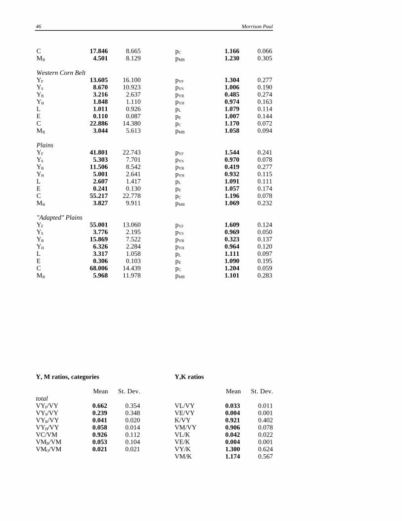
46 Morrison Paul

C 17.846 8.665 pC 1.166 0.066MB 4.501 8.129 pMB 1.230 0.305

Western Corn BeltYF 13.605 16.100 pYF 1.304 0.277YS 8.670 10.923 pYS 1.006 0.190YB 3.216 2.637 pYB 0.485 0.274YH 1.848 1.110 pYH 0.974 0.163L 1.011 0.926 pL 1.079 0.114E 0.110 0.087 pE 1.007 0.144C 22.886 14.380 pC 1.170 0.072MB 3.044 5.613 pMB 1.058 0.094

PlainsYF 41.801 22.743 pYF 1.544 0.241YS 5.303 7.701 pYS 0.970 0.078YB 11.506 8.542 pYB 0.419 0.277YH 5.001 2.641 pYH 0.932 0.115L 2.607 1.417 pL 1.091 0.111E 0.241 0.130 pE 1.057 0.174C 55.217 22.778 pC 1.196 0.078MB 3.827 9.911 pMB 1.069 0.232

"Adapted" PlainsYF 55.001 13.060 pYF 1.609 0.124YS 3.776 2.195 pYS 0.969 0.050YB 15.869 7.522 pYB 0.323 0.137YH 6.326 2.284 pYH 0.964 0.120L 3.317 1.058 pL 1.111 0.097E 0.306 0.103 pE 1.090 0.195C 68.006 14.439 pC 1.204 0.059MB 5.968 11.978 pMB 1.101 0.283

Y, M ratios, categories Y,K ratios

Mean St. Dev. Mean St. Dev.totalVYF/VY 0.662 0.354 VL/VY 0.033 0.011VYS/VY 0.239 0.348 VE/VY 0.004 0.001VYB/VY 0.041 0.020 K/VY 0.921 0.402VYH/VY 0.058 0.014 VM/VY 0.906 0.078VC/VM 0.926 0.112 VL/K 0.042 0.022VMB/VM 0.053 0.104 VE/K 0.004 0.001VMO/VM 0.021 0.021 VY/K 1.300 0.624

VM/K 1.174 0.567


MB=0VYF/VY 0.557 0.441 VL/VY 0.029 0.013VYS/VY 0.348 0.431 VE/VY 0.003 0.001VYB/VY 0.038 0.022 K/VY 0.868 0.434VYH/VY 0.057 0.007 VM/VY 0.913 0.091VC/VM 0.988 0.008 VL/K 0.044 0.034VMB/VM 0.000 0.000 VE/K 0.004 0.002VMO/VM 0.012 0.008 VY/K 1.528 0.939

VM/K 1.396 0.875

MB largeVYF/VY 0.878 0.030 VL/VY 0.037 0.003VYS/VY 0.034 0.017 VE/VY 0.003 0.001VYB/VY 0.035 0.004 K/VY 0.723 0.148VYH/VY 0.053 0.022 VM/VY 0.896 0.030VC/VM 0.650 0.068 VL/K 0.054 0.011VMB/VM 0.313 0.065 VE/K 0.004 0.001VMO/VM 0.037 0.029 VY/K 1.443 0.308

VM/K 1.293 0.279

YF=0VYF/VY 0.000 0.000 VL/VY 0.016 0.004VYS/VY 0.894 0.020 VE/VY 0.003 0.001VYB/VY 0.044 0.023 K/VY 0.859 0.306VYH/VY 0.062 0.007 VM/VY 0.971 0.066VC/VM 0.996 0.004 VL/K 0.020 0.008VMB/VM 0.000 0.000 VE/K 0.003 0.001VMO/VM 0.004 0.004 VY/K 1.300 0.430

VM/K 1.250 0.384

YS=0VYF/VY 0.929 0.013 VL/VY 0.039 0.007VYS/VY 0.000 0.000 VE/VY 0.004 0.002VYB/VY 0.015 0.015 K/VY 0.922 0.679VYH/VY 0.056 0.006 VM/VY 0.947 0.067VC/VM 0.968 0.027 VL/K 0.070 0.044VMB/VM 0.010 0.024 VE/K 0.005 0.002VMO/VM 0.023 0.013 VY/K 1.914 1.366

VM/K 1.791 1.245

Y, M ratios, regions Y,K ratios

WestVYF/VY 0.598 0.317 VL/VY 0.036 0.014VYS/VY 0.306 0.297 VE/VY 0.004 0.002VYB/VY 0.046 0.021 K/VY 0.955 0.472VYH/VY 0.051 0.012 VM/VY 0.870 0.049VC/VM 0.872 0.151 VL/K 0.041 0.014VMB/VM 0.109 0.145 VE/K 0.005 0.001VMO/VM 0.020 0.009 VY/K 1.292 0.534

VM/K 1.126 0.466

Western Corn BeltVYF/VY 0.494 0.423 VL/VY 0.030 0.012VYS/VY 0.410 0.415 VE/VY 0.003 0.002VYB/VY 0.039 0.024 K/VY 0.927 0.443VYH/VY 0.057 0.008 VM/VY 0.917 0.066

48 Morrison Paul

VC/VM 0.918 0.106 VL/K 0.037 0.019VMB/VM 0.069 0.102 VE/K 0.004 0.001VMO/VM 0.015 0.012 VY/K 1.300 0.534

VM/K 1.187 0.469

PlainsVYF/VY 0.775 0.271 VL/VY 0.034 0.008VYS/VY 0.125 0.265 VE/VY 0.003 0.001VYB/VY 0.041 0.017 K/VY 0.847 0.274VYH/VY 0.059 0.012 VM/VY 0.910 0.086VC/VM 0.941 0.102 VL/K 0.046 0.026VMB/VM 0.038 0.090 VE/K 0.004 0.001VMO/VM 0.021 0.017 VY/K 1.363 0.694

VM/K 1.234 0.639

"Adapted" PlainsVYF/VY 0.862 0.022 VL/VY 0.035 0.005VYS/VY 0.034 0.014 VE/VY 0.003 0.001VYB/VY 0.045 0.015 K/VY 0.854 0.166VYH/VY 0.059 0.014 VM/VY 0.887 0.076VC/VM 0.919 0.122 VL/K 0.043 0.010VMB/VM 0.056 0.108 VE/K 0.004 0.001VMO/VM 0.025 0.020 VY/K 1.220 0.265

VM/K 1.078 0.227


C. ADDITIONAL MEASURES FOR

CATEGORIES AND REGIONS

50 Morrison Paul

TABLE C1: COEFFICIENT ESTIMATES

estimate t-statistic

r1-0.0192 -8.267

r2-0.0185 -7.188

r3-0.0238 -10.419

f1-0.0207 -11.411

f2-0.0183 -9.790

f3-0.0133 -6.548

f40.0002 0.053

f5-0.0084 -3.915

LE-0.1442 -1.545

LMB1.1374 6.945

EMB-0.2848 -1.748

LL-0.8823 -6.852

EE0.5018 3.857

MBMB-0.3460 -0.762

LK-0.0827 -1.619

EK-0.1053 -2.065

MBK0.0522 0.463

LYF0.1091 12.032

EYF0.0757 8.048

MBYF1.1632 75.389

LYS0.0194 2.414

EYS0.0227 2.708

MBYS0.8708 60.713

LYB0.1018 12.807

EYB0.1310 16.166

MBYB0.2545 20.252

LYH0.0807 4.561

EYH0.1291 7.205

MBYH0.5584 22.544

LC-0.0011 -0.151

EC-0.0218 -2.875

MBC-0.9657 -77.758

LMO-0.8209 -6.105

EMO-0.9580 -7.120

MBMO-0.3841 -2.377

YFYF-0.0023 -6.925

YSYS0.0006 1.608

YBYB-0.0042 -10.787

YHYH-0.0160 -5.614

KK-0.0139 -1.326

CC-0.0014 -5.411

MOMO-0.0217 -1.106

YFYS-0.0010 -4.011

YFYH-0.0009 -3.958

YFYB-0.0003 -1.210

YSYB-0.0001 -0.317

estimate t-statistic

YSYH-0.0001 -0.499

YBYH-0.0013 -5.207

YFK0.0006 0.222

YSK-0.00001 -0.004

YHK0.0085 4.211

YBK0.0055 2.375

CYF0.0030 5.778

MOYF0.0073 2.876

CYS0.0011 2.198

MOYS0.0034 1.695

CYB0.0006 1.489

MOYB0.0053 2.570

CYH0.0039 6.521

MOYH0.0217 6.865

CK0.0026 1.296

MOK0.0811 2.104

CMO-0.0074 -3.690

MB00.1414 2.427

MBL0.2587 2.670

MBI+I241.0593 4.774

C0.0004 3.870

CCS2-0.0007 -1.970

CCS0.0973 6.042

CQU0.1205 10.441

C1.1981 44.644

CNB-0.0089 -6.417

CP0.6934 3.056

N-12.4480 -15.114

E0.9132 2.299

t1-0.1304 -5.483

t2-0.1542 -6.483

t3-0.1780 -7.486

t4-0.1740 -7.320

t5-0.1794 -7.550

t6-0.1654 -6.970

t7-0.1691 -7.126

t8-0.1357 -5.720

t9-0.1055 -4.444

t10-0.0850 -3.582

t11-0.0657 -2.760

YF-0.0046 -10.681

YF0-0.4771 -23.199

YS-0.0008 -0.591

YS00.0574 3.078


YH0.0032 0.254

regions: r1= WCB, r2= West, r3=Plains (East left out)months: t1=May, t2=JuneδMB0 is associated with a dummy for MB=0 plants, δMBL is for MB large plants

δYS0 is associated with a dummy for YS=0 plants, and similarly for δYF0 for YF=0 plants

δΝ and δE are dummy coefficients for two plants in the cost equation that were outliers

δMBI is associated with a dummy for a plant that was an MB outlier

δfi are associated with dummy variables for the firms

52 Morrison Paul

TABLE C2: SCALE ECONOMIES AND PRICE RATIOS –CATEGORIES AND REGIONS

CATEGORY

Mean St. Dev. Min. Max. Mean St. Dev. Min. Max.total totalεS

TCY 0.919 0.149 0.414 1.974 PSratC 0.987 0.009 0.958 1.002εL

TCY 1.022 0.076 0.806 1.418 MCIrat 0.978 0.019 0.860 1.053εC

TCY 0.947 0.060 0.732 1.245 PratY 1.087 0.075 1.005 1.343εn

TCY 0.949 0.147 0.460 2.081 PIratT 1.062 0.062 0.947 1.279SCFS 0.008 0.009 0.000 0.051 PROF 1.004 0.068 0.794 1.376

MB=0 MB=0εS

TCY 0.899 0.108 0.711 1.604 PSratC 0.988 0.007 0.971 0.997εL

TCY 1.002 0.055 0.891 1.253 MCIrat 0.982 0.010 0.951 0.996εC

TCY 0.952 0.055 0.827 1.179 PratY 1.065 0.059 1.006 1.233εn


MB large MB largeεS

TCY 0.868 0.074 0.690 0.990 PSratC 0.982 0.007 0.967 0.993εL

TCY 1.088 0.113 0.971 1.418 MCIrat 0.971 0.012 0.936 0.986εC

TCY 0.922 0.040 0.821 0.987 PratY 1.155 0.065 1.066 1.343εn


YF=0 YF=0εS

TCY 0.946 0.080 0.799 1.126 PSratC 0.993 0.003 0.986 0.997εL

TCY 0.982 0.056 0.891 1.098 MCIrat 0.987 0.008 0.967 0.996εC

TCY 0.972 0.056 0.881 1.089 PratY 1.013 0.006 1.006 1.024εn


YS=0 YS=0εS

TCY 0.899 0.064 0.772 1.017 PSratC 0.988 0.008 0.971 0.997εL

TCY 1.022 0.046 0.952 1.095 MCIrat 0.984 0.010 0.960 0.996εC

TCY 0.959 0.014 0.931 0.982 PratY 1.076 0.054 1.014 1.191εn


REGION

Mean St. Dev. Min. Max. Mean St. Dev. Min. Max.West WestεS

TCY 1.000 0.151 0.799 1.613 PSratC 0.996 0.004 0.985 1.002


εLTCY 0.976 0.059 0.806 1.067 MCIrat 0.990 0.010 0.939 1.016

εCTCY 0.946 0.042 0.812 1.026 PratY 1.037 0.042 1.005 1.155

εnTCY 1.017 0.151 0.802 1.628 PIratT 1.026 0.039 0.947 1.129

SCFS 0.008 0.007 0.000 0.026 PROF 0.972 0.061 0.794 1.082

WCB WCBεS

TCY 0.929 0.068 0.803 1.106 PSratC 0.992 0.005 0.978 0.998εL

TCY 0.991 0.047 0.891 1.095 MCIrat 0.986 0.009 0.960 0.997εC

TCY 0.961 0.041 0.881 1.081 PratY 1.045 0.045 1.006 1.161εn


Plains PlainsεS

TCY 0.888 0.176 0.414 1.974 PSratC 0.981 0.009 0.958 0.997εL

TCY 1.050 0.081 0.926 1.418 MCIrat 0.969 0.020 0.860 1.053εC

TCY 0.934 0.072 0.732 1.245 PratY 1.131 0.073 1.006 1.343εn


"Adapted" Plains "Adapted" PlainsεS

TCY 0.862 0.194 0.414 1.974 PSratC 0.977 0.008 0.958 0.997εL

TCY 1.062 0.093 0.961 1.418 MCIrat 0.961 0.021 0.860 1.053εC

TCY 0.909 0.073 0.732 1.245 PratY 1.170 0.052 1.077 1.343εn


54 Morrison Paul

TABLE C3: SCOPE AND LABOR ELASTICITIES –CATEGORIES AND REGIONS

Mean St. Dev. Min. Max. Mean St. Dev. Min. Max.total totalSCPFH 0.010 0.010 0.000 0.054 εLC -1.002 1.310 -6.524 0.725SCPFB 0.007 0.009 0.000 0.046 εLYF 0.927 0.611 -0.799 2.067SCPSB 0.000 0.000 0.000 0.002 εLYS 0.807 1.752 -0.100 8.541SCPSH 0.000 0.000 0.000 0.002 εLpL -0.665 0.718 -3.773 -0.076SCPBH 0.004 0.004 0.000 0.022 εLpE -0.095 0.103 -0.548 -0.012SCPFSB 0.015 0.015 0.000 0.065 εLpMB 0.760 0.820 0.088 4.312

εLK 0.153 0.441 -0.815 2.246

MB=0 MB=0SCPFH 0.007 0.007 0.000 0.025 εLC -1.437 1.472 -6.051 0.076SCPFB 0.005 0.008 0.000 0.032 εLYF 0.827 0.688 0.000 2.001SCPSB 0.000 0.001 0.000 0.002 εLYS 1.338 2.023 -0.018 8.289SCPSH 0.000 0.000 0.000 0.002 εLpL -0.894 0.932 -3.773 -0.112SCPBH 0.003 0.004 0.000 0.017 εLpE -0.132 0.137 -0.548 -0.016SCPFSB 0.007 0.010 0.000 0.042 εLpMB 1.025 1.069 0.129 4.312

εLK -0.020 0.273 -0.815 0.612

MB large MB largeSCPFH 0.018 0.012 0.007 0.054 εLC 0.083 0.249 -0.461 0.618SCPFB 0.010 0.005 0.003 0.024 εLYF 0.499 0.454 -0.799 1.096SCPSB 0.000 0.000 0.000 0.000 εLYS -0.021 0.017 -0.077 -0.001SCPSH 0.000 0.000 0.000 0.001 εLpL -0.181 0.073 -0.336 -0.076SCPBH 0.005 0.003 0.001 0.013 εLpE -0.024 0.008 -0.042 -0.012SCPFSB 0.025 0.012 0.004 0.052 εLpMB 0.205 0.081 0.088 0.378

εLK 0.605 0.785 -0.009 2.246

YF=0 YF=0SCPFH 0.000 0.000 0.000 0.000 εLC -2.978 1.636 -6.524 -0.986SCPFB 0.000 0.000 0.000 0.000 εLYF 0.000 0.000 0.000 0.000SCPSB 0.001 0.001 0.000 0.002 εLYS 3.834 1.973 1.245 8.541SCPSH 0.001 0.000 0.000 0.002 εLpL -1.606 0.758 -3.773 -0.797SCPBH 0.001 0.001 0.000 0.003 εLpE -0.239 0.109 -0.548 -0.105SCPFSB 0.001 0.001 0.000 0.002 εLpMB 1.845 0.866 0.918 4.312

εLK -0.227 0.137 -0.815 -0.024

YS=0 YS=0SCPFH 0.009 0.006 0.002 0.023 εLC -0.589 0.223 -1.065 -0.195SCPFB 0.003 0.003 0.000 0.010 εLYF 1.444 0.318 0.903 2.067SCPSB 0.000 0.000 0.000 0.000 εLYS 0.000 0.000 0.000 0.000SCPSH 0.000 0.000 0.000 0.000 εLpL -0.565 0.465 -1.723 -0.112SCPBH 0.001 0.002 0.000 0.005 εLpE -0.081 0.066 -0.224 -0.014SCPFSB 0.003 0.003 0.000 0.010 εLpMB 0.646 0.530 0.129 1.947

εLK -0.013 0.172 -0.378 0.250

REGION

Mean St. Dev. Min. Max. Mean St. Dev. Min. Max.West WestSCPFH 0.004 0.003 0.000 0.011 εLC -0.540 0.629 -2.010 0.227SCPFB 0.003 0.003 0.000 0.011 εLYF 0.860 0.491 0.000 1.686


SCPSB 0.000 0.000 0.000 0.002 εLYS 0.540 0.916 -0.020 2.822SCPSH 0.000 0.000 0.000 0.001 εLpL -0.934 0.676 -2.449 -0.191SCPBH 0.001 0.001 0.000 0.003 εLpE -0.130 0.102 -0.370 -0.025SCPFSB 0.011 0.007 0.001 0.027 εLpMB 1.064 0.777 0.216 2.818

εLK -0.060 0.150 -0.308 0.260

WCB WCBSCPFH 0.004 0.005 0.000 0.017 εLC -1.338 1.768 -6.524 0.200SCPFB 0.002 0.003 0.000 0.012 εLYF 0.724 0.660 0.000 1.864SCPSB 0.000 0.000 0.000 0.002 εLYS 1.471 2.261 -0.033 8.541SCPSH 0.000 0.001 0.000 0.002 εLpL -1.137 0.961 -3.773 -0.141SCPBH 0.001 0.001 0.000 0.005 εLpE -0.160 0.135 -0.548 -0.021SCPFSB 0.007 0.009 0.000 0.041 εLpMB 1.297 1.094 0.162 4.312

εLK -0.088 0.167 -0.426 0.320

Plains PlainsSCPFH 0.016 0.010 0.000 0.054 εLC -0.970 1.143 -5.867 0.725SCPFB 0.012 0.010 0.000 0.046 εLYF 1.048 0.582 -0.799 2.067SCPSB 0.000 0.000 0.000 0.002 εLYS 0.445 1.415 -0.100 7.092SCPSH 0.000 0.000 0.000 0.002 εLpL -0.352 0.393 -1.723 -0.076SCPBH 0.006 0.005 0.000 0.022 εLpE -0.052 0.059 -0.260 -0.012SCPFSB 0.022 0.016 0.000 0.065 εLpMB 0.403 0.451 0.088 1.972

εLK 0.350 0.511 -0.815 2.246

"Adapted" Plains "Adapted" PlainsSCPFH 0.021 0.007 0.012 0.054 εLC -0.558 0.443 -1.493 0.725SCPFB 0.017 0.008 0.006 0.046 εLYF 1.008 0.529 -0.799 1.811SCPSB 0.000 0.000 0.000 0.001 εLYS -0.016 0.020 -0.100 0.022SCPSH 0.000 0.000 0.000 0.001 εLpL -0.159 0.040 -0.242 -0.076SCPBH 0.009 0.004 0.002 0.022 εLpE -0.023 0.007 -0.055 -0.012SCPFSB 0.032 0.012 0.010 0.065 εLpMB 0.183 0.046 0.088 0.287

εLK 0.586 0.483 -0.111 2.246

56 Morrison Paul

TABLE C4: ENERGY AND C SHADOW VALUEELASTICITIES – CATEGORIES ANDREGIONS

Mean St. Dev. Min. Max. Mean St. Dev. Min. Max.total totalεEC -13.052 10.017 -64.605 5.287 εZCC 0.308 0.203 0.034 0.831εEYF 5.323 6.193 -26.563 21.917 εZCYF -0.246 0.217 -0.919 0.000εEYS 5.310 11.201 -1.385 55.813 εZCYS -0.019 0.025 -0.110 0.000εEpL 2.565 2.795 0.374 15.150 εZCpL 0.026 0.022 -0.049 0.093εEpE -0.873 0.947 -5.316 -0.130 εZCpE 0.044 0.022 -0.021 0.121εEpMB -1.692 1.853 -10.207 -0.244 εZCpMB 0.930 0.043 0.787 1.069εEK 1.576 5.463 -4.832 37.651 εZCK -0.030 0.020 -0.087 -0.002

MB=0 MB=0εEC -18.023 10.876 -50.512 -3.643 εZCC 0.252 0.148 0.056 0.634εEYF 6.416 6.531 -1.603 21.917 εZCYF -0.164 0.168 -0.603 0.000εEYS 9.159 13.346 -0.193 49.742 εZCYS -0.022 0.030 -0.108 0.000εEpL 3.331 3.619 0.591 15.150 εZCpL 0.032 0.017 -0.005 0.074εEpE -1.114 1.175 -4.944 -0.188 εZCpE 0.052 0.016 0.017 0.100εEpMB -2.217 2.445 -10.207 -0.403 εZCpMB 0.917 0.032 0.827 0.988εEK -0.294 2.566 -4.832 6.886 εZCK -0.022 0.015 -0.068 -0.003

MB large MB largeεEC -2.465 3.445 -9.799 5.287 εZCC 0.405 0.173 0.152 0.769εEYF -1.332 7.583 -26.563 7.430 εZCYF -0.472 0.195 -0.919 -0.195εEYS -0.254 0.295 -1.385 0.037 εZCYS -0.012 0.007 -0.025 0.000εEpL 0.941 0.309 0.470 1.514 εZCpL -0.007 0.018 -0.049 0.029εEpE -0.311 0.101 -0.499 -0.157 εZCpE 0.014 0.018 -0.021 0.050εEpMB -0.630 0.208 -1.015 -0.312 εZCpMB 0.993 0.036 0.924 1.069εEK 7.984 11.282 -0.524 37.651 εZCK -0.047 0.022 -0.087 -0.021

YF=0 YF=0εEC -26.358 11.531 -64.605 -8.227 εZCC 0.16 0.073 0.1 0.29εEYF 0.000 0.000 0.000 0.000 εZCYF 0.000 0.000 0.000 0.000εEYS 25.100 11.713 7.586 55.813 εZCYS -0.059 0.027 -0.110 -0.02εEpL 4.970 3.654 1.765 15.150 εZCpL 0.046 0.017 0.023 0.078εEpE -1.680 1.175 -4.944 -0.623 εZCpE 0.064 0.017 0.042 0.102εEpMB -3.290 2.480 -10.207 -1.142 εZCpMB 0.890 0.033 0.827 0.931εEK -2.126 0.910 -4.832 -0.691 εZCK -0.014 0.008 -0.024 -0.003

YS=0 YS=0εEC -13.916 7.313 -29.005 -4.115 εZCC 0.244 0.166 0.058 0.632εEYF 12.328 5.597 5.093 21.917 εZCYF -0.205 0.145 -0.523 -0.040εEYS 0.000 0.000 0.000 0.000 εZCYS 0.000 0.000 0.000 0.000εEpL 3.021 2.712 0.697 9.137 εZCpL 0.025 0.007 0.012 0.037εEpE -0.995 0.890 -2.982 -0.233 εZCpE 0.045 0.008 0.023 0.055εEpMB -2.026 1.822 -6.155 -0.463 εZCpMB 0.930 0.014 0.908 0.965εEK -0.293 2.173 -3.160 3.565 εZCK -0.016 0.009 -0.026 -0.007

REGION

Mean St. Dev. Min. Max. Mean St. Dev. Min. Max.West WestεEC -7.934 5.357 -24.221 -0.237 εZCC 0.14 0.07 0.0 0.309εEYF 4.837 4.349 -4.100 17.138 εZCYF -0.113 0.12 -0.423 0.00


εEYS 3.652 5.568 -0.238 23.337 εZCYS -0.015 0.013 -0.045 -0.002εEpL 3.314 2.448 1.091 14.099 εZCpL 0.015 0.015 -0.02 0.036εEpE -1.133 0.945 -5.316 -0.356 εZCpE 0.033 0.015 0.002 0.059εEpMB -2.181 1.511 -8.783 -0.735 εZCpMB 0.952 0.030 0.907 1.017εEK -0.742 1.498 -2.929 3.125 εZCK -0.015 0.008 -0.027 -0.005

WCB WCBεEC -14.812 13.322 -64.605 -1.249 εZCC 0.18 0.117 0.0 0.507εEYF 3.973 4.163 0.000 13.280 εZCYF -0.120 0.144 -0.498 0.000εEYS 10.249 14.176 -0.330 55.813 εZCYS -0.025 0.031 -0.110 0.00εEpL 4.345 4.022 0.681 15.150 εZCpL 0.025 0.022 -0.014 0.078εEpE -1.466 1.327 -4.944 -0.225 εZCpE 0.043 0.023 0.006 0.102εEpMB -2.880 2.698 -10.207 -0.456 εZCpMB 0.931 0.044 0.834 1.008εEK -1.154 1.626 -4.832 3.429 εZCK -0.019 0.014 -0.054 -0.002

Plains PlainsεEC -13.740 8.462 -49.765 5.287 εZCC 0.438 0.189 0.058 0.831εEYF 5.900 7.391 -26.563 21.917 εZCYF -0.368 0.212 -0.919 0.000εEYS 2.560 8.640 -1.385 49.742 εZCYS -0.016 0.022 -0.105 0.000εEpL 1.477 1.562 0.374 9.137 εZCpL 0.030 0.023 -0.049 0.093εEpE -0.504 0.521 -2.982 -0.130 εZCpE 0.048 0.022 -0.021 0.121εEpMB -0.973 1.042 -6.155 -0.244 εZCpMB 0.922 0.045 0.787 1.069εEK 3.838 6.622 -4.466 37.651 εZCK -0.041 0.021 -0.087 -0.007

"Adapted" Plains "Adapted" PlainsεEC -10.609 5.927 -30.078 5.287 εZCC 0.548 0.118 0.333 0.831εEYF 4.082 7.120 -26.563 18.302 εZCYF -0.490 0.136 -0.919 -0.277εEYS -0.164 0.287 -1.385 0.261 εZCYS -0.012 0.007 -0.041 -0.003εEpL 0.772 0.204 0.374 1.298 εZCpL 0.024 0.025 -0.049 0.093εEpE -0.265 0.082 -0.482 -0.130 εZCpE 0.043 0.023 -0.021 0.121εEpMB -0.506 0.128 -0.851 -0.244 εZCpMB 0.933 0.047 0.787 1.069εEK 6.347 7.092 -2.557 37.651 εZCK -0.055 0.012 -0.087 -0.035

58 Morrison Paul

TABLE C5: INPUT SUPPLY AND COST ECONOMYELASTICITIES – CATEGORIES ANDREGIONS

Mean St. Dev. Min. Max. Mean St. Dev. Min. Max.total totalεpCC 0.013 0.009 -0.002 0.039 εTCY,C 0.252 0.242 -0.127 1.538εpCNOB -0.023 0.034 -0.130 0.000 εTCY,YF -0.240 0.243 -1.251 0.143εpCPRC 0.010 0.015 -0.022 0.062 εTCY,YS 0.014 0.053 -0.126 0.201εpCQU 0.095 0.019 0.000 0.144 εTCY,pL 0.032 0.034 -0.085 0.125εpCCS 0.003 0.011 0.000 0.073 εTCY,pE 0.051 0.033 -0.067 0.143 εTCY,pMB 0.824 0.109 0.514 1.518 εTCY,K -0.021 0.037 -0.248 0.019

MB=0 MB=0εpCC 0.011 0.007 0.003 0.028 εTCY,C 0.154 0.192 -0.127 1.014εpCNOB -0.027 0.034 -0.103 0.000 εTCY,YF -0.131 0.170 -0.697 0.106εpCPRC 0.013 0.017 0.000 0.057 εTCY,YS 0.038 0.061 -0.021 0.201εpCQU 0.102 0.008 0.079 0.144 εTCY,pL 0.040 0.026 -0.039 0.098εpCCS 0.000 0.001 0.000 0.005 εTCY,pE 0.060 0.027 -0.029 0.134

εTCY,pMB 0.882 0.083 0.640 1.518 εTCY,K -0.008 0.010 -0.064 0.016

MB large MB largeεpCC 0.017 0.007 0.007 0.034 εTCY,C 0.340 0.163 0.121 0.769εpCNOB -0.022 0.046 -0.123 0.000 εTCY,YF -0.463 0.207 -1.018 -0.199εpCPRC 0.008 0.017 0.000 0.051 εTCY,YS -0.011 0.007 -0.028 -0.001εpCQU 0.093 0.015 0.029 0.112 εTCY,pL -0.006 0.025 -0.085 0.036εpCCS 0.000 0.000 0.000 0.001 εTCY,pE 0.013 0.028 -0.067 0.062 εTCY,pMB 0.682 0.077 0.514 0.872 εTCY,K -0.062 0.082 -0.248 -0.007

YF=0 YF=0εpCC 0.007 0.004 0.003 0.015 εTCY,C 0.028 0.081 -0.127 0.201εpCNOB -0.008 0.012 -0.032 0.000 εTCY,YF 0.000 0.000 0.000 0.000εpCPRC 0.005 0.007 0.000 0.030 εTCY,YS 0.104 0.051 -0.020 0.201εpCQU 0.098 0.006 0.079 0.109 εTCY,pL 0.060 0.025 0.015 0.098εpCCS 0.000 0.001 0.000 0.005 εTCY,pE 0.080 0.022 0.048 0.126 εTCY,pMB 0.839 0.052 0.640 1.033 εTCY,K -0.003 0.004 -0.009 0.016

YS=0 YS=0εpCC 0.011 0.007 0.003 0.028 εTCY,C 0.162 0.141 -0.124 0.523εpCNOB -0.037 0.026 -0.076 0.000 εTCY,YF -0.154 0.157 -0.515 0.143εpCPRC 0.014 0.011 0.000 0.037 εTCY,YS 0.000 0.000 0.000 0.000εpCQU 0.103 0.008 0.086 0.121 εTCY,pL 0.039 0.009 0.016 0.069εpCCS 0.000 0.000 0.000 0.000 εTCY,pE 0.065 0.019 0.026 0.107 εTCY,pMB 0.909 0.041 0.834 1.047 εTCY,K -0.013 0.010 -0.049 0.008

REGION

Mean St. Dev. Min. Max. Mean St. Dev. Min. Max.West WestεpCC 0.004 0.004 -0.002 0.013 εTCY,C 0.169 0.178 -0.127 0.873


εpCNOB -0.017 0.018 -0.055 0.000 εTCY,YF -0.139 0.129 -0.484 0.010εpCPRC 0.008 0.009 -0.022 0.023 εTCY,YS 0.009 0.061 -0.117 0.201εpCQU 0.101 0.008 0.083 0.116 εTCY,pL 0.023 0.022 -0.019 0.070εpCCS 0.017 0.025 0.000 0.073 εTCY,pE 0.047 0.019 0.003 0.077 εTCY,pMB 0.740 0.101 0.514 0.954 εTCY,K -0.010 0.009 -0.029 0.005

WCB WCBεpCC 0.008 0.005 0.002 0.022 εTCY,C 0.098 0.116 -0.100 0.447εpCNOB -0.031 0.039 -0.123 0.000 εTCY,YF -0.100 0.139 -0.522 0.073εpCPRC 0.012 0.014 0.000 0.051 εTCY,YS 0.042 0.061 -0.022 0.186εpCQU 0.095 0.016 0.019 0.121 εTCY,pL 0.036 0.029 -0.009 0.098εpCCS 0.000 0.001 0.000 0.005 εTCY,pE 0.056 0.030 0.008 0.126 εTCY,pMB 0.785 0.106 0.548 1.010 εTCY,K -0.008 0.008 -0.049 0.008

Plains PlainsεpCC 0.018 0.008 0.003 0.039 εTCY,C 0.377 0.250 -0.124 1.538εpCNOB -0.014 0.027 -0.086 0.000 εTCY,YF -0.363 0.258 -1.251 0.143εpCPRC 0.007 0.015 0.000 0.062 εTCY,YS -0.003 0.035 -0.126 0.172εpCQU 0.092 0.022 0.000 0.144 εTCY,pL 0.029 0.038 -0.085 0.125εpCCS 0.001 0.003 0.000 0.021 εTCY,pE 0.046 0.036 -0.067 0.134 εTCY,pMB 0.868 0.095 0.613 1.518 εTCY,K -0.028 0.047 -0.248 0.019

"Adapted" Plains "Adapted" PlainsεpCC 0.022 0.007 0.004 0.039 εTCY,C 0.500 0.206 0.092 1.538εpCNOB -0.012 0.028 -0.086 0.000 εTCY,YF -0.502 0.200 -1.251 -0.069εpCPRC 0.007 0.017 0.000 0.062 εTCY,YS -0.012 0.011 -0.066 0.005εpCQU 0.095 0.009 0.061 0.111 εTCY,pL 0.014 0.037 -0.085 0.125εpCCS 0.002 0.004 0.000 0.021 εTCY,pE 0.030 0.033 -0.067 0.116 εTCY,pMB 0.861 0.094 0.613 1.125 εTCY,K -0.038 0.056 -0.248 0.019

60 Morrison Paul

TABLE C6: C "MARKDOWN" AND YF "MARKUP"ELASTICITIES – CATEGORIES ANDREGIONS

Mean St.Dev.

Min. Max. Mean St.Dev.

Min. Max.

total totalεprCC -0.008 0.004 -0.014 0.002 εprYF,C -0.038 0.048 -0.242 0.000εprCYF -0.005 0.007 -0.031 0.000 εprYF,YF 0.132 0.133 0.000 0.667εprCYS 0.000 0.000 -0.002 0.000 εprYF,YS 0.001 0.003 0.000 0.020εprCpMB 0.000 0.001 -0.002 0.004 εprYF,pL -0.005 0.005 -0.036 0.016εprCpL 0.001 0.001 -0.001 0.005 εprYF,pE -0.002 0.004 -0.021 0.026εprCpE 0.013 0.009 -0.002 0.037 εprYF,pMB -0.078 0.069 -0.325 0.000εprCK -0.001 0.001 -0.003 0.000 εprYF,K -0.001 0.001 -0.004 0.000

MB=0 MB=0εprCC -0.008 0.003 -0.013 -0.003 εprYF,C -0.022 0.029 -0.120 0.000εprCYF -0.003 0.004 -0.016 0.000 εprYF,YF 0.085 0.093 0.000 0.358εprCYS 0.000 0.000 -0.001 0.000 εprYF,YS 0.000 0.000 0.000 0.002εprCpMB 0.000 0.000 0.000 0.001 εprYF,pL -0.004 0.004 -0.012 0.000εprCpL 0.001 0.000 0.000 0.002 εprYF,pE -0.002 0.002 -0.007 0.001εprCpE 0.011 0.007 0.003 0.028 εprYF,pMB -0.054 0.055 -0.194 0.000εprCK 0.000 0.000 -0.002 0.000 εprYF,K 0.000 0.001 -0.002 0.000

MB large MB largeεprCC -0.010 0.002 -0.012 -0.006 εprYF,C -0.070 0.056 -0.236 -0.010εprCYF -0.010 0.008 -0.031 -0.002 εprYF,YF 0.264 0.143 0.086 0.667εprCYS 0.000 0.000 -0.001 0.000 εprYF,YS 0.004 0.003 0.000 0.013εprCpMB 0.000 0.000 -0.002 0.001 εprYF,pL -0.003 0.005 -0.010 0.016εprCpL 0.000 0.000 -0.001 0.002 εprYF,pE 0.001 0.006 -0.006 0.026εprCpE 0.018 0.007 0.007 0.037 εprYF,pMB -0.152 0.062 -0.325 -0.065εprCK -0.001 0.001 -0.003 0.000 εprYF,K -0.002 0.001 -0.004 0.000

YF=0 YF=0εprCC -0.006 0.002 -0.010 -0.003 εprYF,C 0.000 0.000 0.000 0.000εprCYF 0.000 0.000 0.000 0.000 εprYF,YF 0.000 0.000 0.000 0.000εprCYS -0.001 0.000 -0.002 0.000 εprYF,YS 0.000 0.000 0.000 0.000εprCpMB 0.000 0.000 0.000 0.001 εprYF,pL 0.000 0.000 0.000 0.000εprCpL 0.001 0.000 0.000 0.001 εprYF,pE 0.000 0.000 0.000 0.000εprCpE 0.007 0.003 0.003 0.012 εprYF,pMB 0.000 0.000 0.000 0.000εprCK 0.000 0.000 0.000 0.000 εprYF,K 0.000 0.000 0.000 0.000

YS=0 YS=0εprCC -0.008 0.004 -0.013 -0.002 εprYF,C -0.025 0.029 -0.107 -0.001εprCYF -0.004 0.004 -0.016 0.000 εprYF,YF 0.104 0.083 0.016 0.297εprCYS 0.000 0.000 0.000 0.000 εprYF,YS 0.000 0.000 0.000 0.000εprCpMB 0.000 0.000 0.000 0.001 εprYF,pL -0.005 0.003 -0.012 -0.001εprCpL 0.001 0.000 0.000 0.002 εprYF,pE -0.003 0.002 -0.006 -0.001εprCpE 0.011 0.008 0.002 0.028 εprYF,pMB -0.067 0.046 -0.162 -0.013εprCK 0.000 0.000 -0.001 0.000 εprYF,K 0.000 0.000 -0.001 0.000

REGION

Mean St.Dev.

Min. Max. Mean St.Dev.

Min. Max.


West WestεprCC -0.004 0.003 -0.010 0.002 εprYF,C -0.007 0.011 -0.044 0.000εprCYF -0.001 0.001 -0.006 0.000 εprYF,YF 0.051 0.061 0.000 0.233εprCYS 0.000 0.000 0.000 0.000 εprYF,YS 0.000 0.000 0.000 0.002εprCpMB 0.000 0.000 0.000 0.000 εprYF,pL -0.002 0.001 -0.004 0.000εprCpL 0.000 0.000 0.000 0.000 εprYF,pE -0.001 0.001 -0.003 0.002εprCpE 0.004 0.004 -0.002 0.015 εprYF,pMB -0.037 0.041 -0.150 0.000εprCK 0.000 0.000 0.000 0.000 εprYF,K 0.000 0.000 -0.001 0.000

WCB WCBεprCC -0.006 0.003 -0.012 -0.002 εprYF,C -0.011 0.018 -0.080 0.000εprCYF -0.002 0.003 -0.011 0.000 εprYF,YF 0.058 0.074 0.000 0.269εprCYS 0.000 0.000 -0.002 0.000 εprYF,YS 0.001 0.001 0.000 0.007εprCpMB 0.000 0.000 0.000 0.001 εprYF,pL -0.002 0.002 -0.008 0.000εprCpL 0.000 0.000 0.000 0.001 εprYF,pE -0.001 0.001 -0.004 0.000εprCpE 0.008 0.005 0.002 0.022 εprYF,pMB -0.039 0.047 -0.157 0.000εprCK 0.000 0.000 -0.001 0.000 εprYF,K 0.000 0.000 -0.002 0.000

Plains PlainsεprCC -0.010 0.003 -0.014 -0.002 εprYF,C -0.065 0.052 -0.242 0.000εprCYF -0.009 0.007 -0.031 0.000 εprYF,YF 0.206 0.136 0.000 0.667εprCYS 0.000 0.000 -0.001 0.000 εprYF,YS 0.002 0.003 0.000 0.020εprCpMB 0.001 0.001 -0.002 0.004 εprYF,pL -0.007 0.006 -0.036 0.016εprCpL 0.001 0.001 -0.001 0.005 εprYF,pE -0.003 0.005 -0.021 0.026εprCpE 0.018 0.009 0.002 0.037 εprYF,pMB -0.117 0.067 -0.325 0.000εprCK -0.001 0.001 -0.003 0.000 εprYF,K -0.001 0.001 -0.004 0.000

"Adapted" Plains "Adapted" PlainsεprCC -0.010 0.003 -0.014 -0.002 εprYF,C -0.092 0.045 -0.242 -0.031εprCYF -0.012 0.007 -0.031 -0.001 εprYF,YF 0.279 0.107 0.121 0.667εprCYS 0.000 0.000 -0.001 0.000 εprYF,YS 0.004 0.003 0.001 0.020εprCpMB 0.001 0.001 -0.002 0.004 εprYF,pL -0.008 0.006 -0.036 0.016εprCpL 0.001 0.001 -0.001 0.005 εprYF,pE -0.003 0.006 -0.021 0.026εprCpE 0.022 0.007 0.003 0.037 εprYF,pMB -0.153 0.046 -0.325 -0.081εprCK -0.001 0.001 -0.003 0.000 εprYF,K -0.002 0.001 -0.004 -0.001

62 Morrison Paul

D. DATA SUPPLEMENT


The data used for this study are specified at the monthly level of time aggregation,allowing a more appropriate connection between output and input data than wouldweekly data. Monthly observations permit a more appropriate link between shipmentsand production (particularly for fabrication, which is often stored longer than carcasses).Monthly data also reduce concerns about outliers due to reporting “errors,” facilitateignoring the differences between hours paid and hours worked as discrepancies areminimized over a month, and allow the use of figures that were (explicitly or implicitly)allocated from monthly numbers in the “weekly” measures reported.

A few anomalies in the data should be raised. Only one firm submitted reports thatdiffered sufficiently from others, and appeared incomplete enough, to be omitted from thesample. Some other plants were outliers, although their differences seemed effectivelyrepresented through dummy fixed effects in the cost function. Among these outliers was aplant that appeared to underreport MB use (as was also true for some other plants from thesame firm, although not as dramatically), thus exhibiting very low costs. In constrast,one other plant had excessively high costs, possibly due to mis-reporting meat packingand other operations, as this is a highly diversified plant. Sensitivity tests for differingtreatments of these and other outlier plants indicated that they increased the volatility ofthe estimates, particularly if not recognized by fixed effects, but they did not alter thesubstantive conclusions about market power and cost economies.

Another issue was the “matchup” of the numbers, due to the incompatibility of thereporting for many of the initial and final months. The anomalies were quite easily seenfrom descriptive statistics (ratios of materials and labor payments to output for abeginning or ending month, for example); observations that were obviously mis-matchedwere deleted from the sample. Final results were reported primarily on observations “2-12,” leaving out the first month of reporting and, often, the final month.

Observation of the data identified clear divisions in the structure of the plants, inaddition to their obvious characterization by size. Plants that sold no fabricated output,or no slaughter output, would be expected to differ from plants that did not specialize inthis manner. Similarly, some plants purchased no (or very little) MB input, whileanother well-defined sub-sample used a large proportion of MB. This difference suggestedthe usefulness of generating results by production structure “category.” The differencealso highlighted the importance of recognizing zero (or nearly zero) input and outputvalues in the econometric model.

Initially, some separate estimation over sub-samples was attempted to deal withthese differences in output and input use among plants. However, estimation using sub-samples that included few plants encountered degrees of freedom problems and causedcomparability difficulties across different types of plants. Results from these trialestimations were close to those obtained when pooling the full sample with fixed effectsincluded. Thus, pooled estimation, with fixed effects (dummy variables) representingdiffering production structures and outliers, was used for the final reported results. The Kvalues also act as plant-specific controls.

Given these comments and qualifications, it is useful to look at Appendix Table B1,that presents summary statistics for the categories (total, plants with MB=0, MB large,YF=0, and YS=0 plants) and regions. The reported numbers present mean (average)values of the measures, their standard deviation (st. dev.), minimum over the sample(min.) and maximum (max.).

The first numbers presented are for total values of output (VY, including fabricated[YF], slaughter [YS], hides [YH] and byproduct [YB] sales), labor use (VL), energy (VE),“materials” input (VM, including cattle [C], purchased beef [MB], and “other” materialsand supplies [MO]), and the estimated value of capital stock services based on the“replacement cost” reported (K), all reported in millions of dollars.

The overall or “total” (average across all plants) measures mask the great sizedifferences across plants. An average plant produces over 55 million dollars worth ofoutput monthly, but many plants vary far from this average. Even though only “large”plants are included in this sample, substantial size variation remains, in addition to thestructural differences.

By far the greatest variable expenditure or opportunity cost is materials, includingcattle and intermediate beef purchases. In fact, 91 percent of the value of output is spent

64 Morrison Paul

on these inputs. Most of that is cattle, for MB averages only 5 percent of materials costs.This is evident in the Y, M, and C ratios.

The K measures indicate that the replacement value of plants is typically slightlyless than the value of output produced each month (although plants that produce morefabricated output also have greater capital costs per unit of output). Approximate capitalcosts per month may be computed from this. Assuming an interest rate of 8.5 percent(the Moody Baa bond yield in 1991), depreciation and maintenance of 10 percent, andallocating across months, we can compute an average monthly capital “user” cost ofabout 1.5 percent of the value of the capital stock K. This procedure for valuing capitalwas used for imputing the optimal level of capital for the estimated long-run elasticitiesreported. However, these somewhat rough estimates of the return to capital were notembodied in the econometric (“short-run”) model.

Plants that purchase or transfer significant amounts of beef (MB large) are the largestat nearly 100 million dollars worth of output per month on average. These large plantsare also associated with the largest firms – both in terms of capital and output value.Plants within any one firm, however, vary considerably in size.

The more specialized plants tend to be smaller than the average; plants with eitherYF=0 or YS=0 are significantly smaller than average (about half and one-third the value oftotal output, respectively). Also, the YF=0 plants use primarily materials inputs –reported labor and energy costs are minimal – and virtually all the “materials” inputs arecattle (C). Plants that do all fabricating (YS=0 plants), by contrast, have a clearly higherlabor to output ratio.

Regional differences are also evident. By far the largest plants are located in thePlains. Plants in the remaining three regions – the East, West and Western Corn Belt –produce less than half the output per plant than the average for the Plains, and typicallyless than one third of that from the “Adapted Plains” plants on average (as defined inAppendix A).

The output and input levels presented in the next section of Table B1 providesome indications of their composition. The numbers in these tables indicate that theplants that do no fabricating also use virtually no MB, and those that only producefabricated products use high levels of MB. That is, in general, the plants that use no MB

have a relatively high proportion of slaughter (YS) output, and those with high MB

demand levels produce a much greater proportion of YF output.Information about price levels is also presented in this section of Table B1.

Although these values provide some indication of deviations above and below a pricelevel of 1.0, it should be noted that “prices” for firms that produce or use no output orinput were assumed to face corresponding prices of 1.0. This assumption was made forestimation purposes; it makes no sense to assume that plants that purchase no MB face azero price for this input. Implicitly, the decision to produce/demand an output/input isassumed to be separate from that price – they face approximately the average price.

Although this is conceptually reasonable, it makes the interpretation of prices in thistable somewhat misleading as price measures for specialized plants will be biased towardone. Nevertheless, information may still be drawn from these numbers. First, prices aresurprisingly consistent across categories, firms, and regions in terms of the means,although considerable variation within these categories is indicated by the standarddeviations. But since these values are expressed in terms of pounds of product, variationlikely indicates differences in type of output.

Across regions, it seems plants in the Plains, especially the MB large plants, receivethe highest prices for YF. Even without referring to the econometric results, fabricationappears profitable for the large Plains plants and firms.

Also, prices of MB are highest, on average, for firms that use a significant amount ofthis input. Plants in the “Adapted Plains” category and, especially, those in the West,face relatively high prices for MB inputs. Also, plants that produce only fabricatedproducts exhibit slightly higher prices for cattle (C) input, as do the Plains and,particularly, the “Adapted Plains” plants.

The Y and M ratios presented in the third section of Table B1 highlight the outputand input composition patterns indicated by the value, quantity and price levels. Plantswith large MB purchases produce by far the most fabricated as opposed to slaughter


output, with YF comprising 87 percent of the value of output. In reverse, plants withMB=0 average 35 percent slaughter output in terms of value, compared to a 24 percentoverall average.

Plains plants, particularly the large ones, tend to produce both YS and YF withemphasis on fabrication; they purchase a significant amount of beef products, MB.Meanwhile, the small specialized plants mostly do their own slaughtering and eithermarket their product directly as slaughter output or use it for fabrication.

As might be expected, the YH to total output ratio is very constant, averaging around6 percent. The MO to total M ratio also is quite consistent at about 2 percent (althoughplants producing more YF have greater packaging and other materials costs).

Finally, consider the ratios of inputs to output and capital values – the Y,K ratios inTable B1. Note that plants with high MB levels tend to have low capital-to-outputratios, as do plants associated with most firms in the Plains region. These low K, Yratios are striking in that they are associated with the largest plants. This provides someindication that larger plants are more efficient in terms of output production – the verybasis for cost economies. Labor intensity is much more consistent across plants,although high for plants in the East, and low for plants with no sales of fabricatedproducts.

Overall, considerable variation, but also strong similarities appear in the data acrosscategories, firms, and regions. This suggests that estimation of input and output patternsin the industry may usefully be carried out by pooling these data, while recognizing thedifferences in structure that cause variations, such as specialization in particular types ofoutputs or inputs. The legitimacy of pooling these data, while recognizing between-plantdifferences, is validated by model results. Although dummy variables reflectingcategories, firms, and regions are statistically significant, they are not large in magnitude.And the results for various specifications and data sub-samples provided a very robuststory about production structure in this industry.

cost economies and market power in u.s. beef packingcost economies and market power. the...

Documents