Cost Characterizations of Supply Chain Delivery Performance

Alfred L. Guiffrida and Rakesh Nagi* Department of Industrial Engineering

342 Bell Hall University at Buffalo (SUNY)

Buffalo, New York 14260 USA

Abstract This paper addresses strategies for improving delivery performance in a serial supply chain when delivery performance is evaluated with respect to a delivery window. Contemporary management theories advocate the reduction of variance as a key step in improving the overall performance of a system. Models are developed that incorporate the variability found in the individual stages of the supply chain into a financial measure that serves as a benchmark for justifying the capital investment required to improve delivery performance within the supply chain to meet a targeted goal. Key Words: Improving Delivery Performance, Justifying Variance Reduction Paper Received January 2004 Revised October 2004 Accepted January 2005 *Corresponding Author: E-mail: nagi@buffalo.edu Phone: 716-645-2357 ext. 2103 Fax: 716-645-3302

Cost Characterizations of Supply Chain Delivery Performance

1. Introduction In the past three decades, the relationship between customers, manufacturers and suppliers has undergone numerous paradigmatic changes. Modern manufacturing paradigms such as the Just-In-Time (JIT) philosophy, Total Quality Management (TQM) and agile manufacturing, advocate the elimination of non-value adding activities in procurement, production and distribution. The progressive approach espoused by these paradigms is to view individual actions as part of an integrated series of business functions that span across the entire supply chain. The goals of supply chain management are to reduce uncertainty and risks in the supply chain, thereby positively affecting inventory levels, cycle time, processes, and ultimately, end-customer service levels (Chase et al., 1998). Effective supply chain administration requires a proactive management style focused on long-term continuous improvement of the supply chain. Performance measures that accurately reflect supply chain operations are required to support continuous improvement within a supply chain. Doing so requires the adoption of performance metrics that accurately measure the supply chain as a whole, and that focus on measuring performance in terms of cost and uncertainty. Several researchers have expressed concern regarding limitations in supply chain performance metrics (see for example, Gunasekaran et al., 2004). These concerns are three-fold. First, performance measures are not cost based. Ellram (2002) identified the lack of relevant performance measures as a key barrier to successful cost management in the supply chain. This view is also shared by Lancioni (2000), who observes that as the importance of supply chain management grows, it becomes even more imperative for firms to measure the cost performance of their supply chain systems. Lalonde and Pohlen (1996) identified a critical need in supply chain management for linking performance measurement with cost. Practicing managers in business would agree that cost analysis is important in the management, planning and control of their organizations. Because the metric of cost is easily understood and routinely welcomed by management, cost-based performance measures are attractive for use in supply chain management. Cost-based performance measures are compatible across various processes and stages of the supply chain. Cost-based measures also provide direct input into the capital budgeting processes used to justify investment in supply chain improvement initiatives. In a case study of five firms Ellram (2002) found: 1) cost consciousness is a way of life in the organizations studied, and 2) this philosophy was felt and experienced by all members of the corporation, from the chairman of the board, to the administrative staff, even to the workers on the manufacturing floor. Ballou et al. (2000) cite the ability to define and measure cost among channel members as the first step to analyze the supply chain for cost-saving opportunities.

1

Second, performance measures often ignore variability. Variability is inherent in nearly all manufacturing and distributions systems. Managing uncertainty is one of the most important and challenging problems to effective supply chain management (Blackhurst et al., 2004; Sabri and Beamon, 2000). Johnson and Davis (1998) expressed concern that current supply chain performance metrics measure attributes that customarily ignore the effects of variability. The reduction of variance is a critical aspect to a methodology designed to improve system performance (Johnson and Davis, 1998; Davis, 1993). Lastly, the adoption of performance metrics that accurately measure the supply chain as a whole, and that focus on measuring performance in terms of cost and uncertainty must be integrated into chain-wide continuous improvement activities. Walker and Alber (1999) note that supply chain performance measures continue to be strictly defined in terms that not only optimize local operations, but also reward the individual performance of chain members. Van Hoek (1998) concludes that current performance measures are designed for single members within the supply chain and do not reach across chain members. Cooper et al. (1997) identify that shortcomings in performance measurement limit improvement projects between supply chain members. Therefore, the performance measures used must be formulated to serve as integrating tools for fostering long term, continuous improvement between and within the various stages of the supply chain. Aspects of supply chain operation that are not measured in understandable performance metrics such as cost will clearly hinder cooperation between the various coalitions found within the supply chain structure. Performance analysis that is based on cost is not an end in itself. When used in combination with non-cost based measures, such as those found in the balanced score card methodology, cost-based measures, designed to measure processes linking various stages of the supply chain, will prove an effective performance measure for long term improvement in supply chain operations. Cost-based analysis should be viewed as an ongoing initiative incorporated into a framework that connects functional areas and organizations within the supply chain into a reward system for never-ending improvement. In this research we concentrate on one aspect of overall supply chain performance, delivery timeliness to the final customer in a serial supply chain that is operating under a centralized management structure. The objectives of this paper are as follows: 1) develop a cost-based performance metric for analyzing delivery performance within a supply chain, and ii) develop a framework for integrating delivery accuracy and reliability into the continuous improvement of supply chain operations. In satisfying the first research objective, a cost-based performance metric for evaluating delivery performance and reliability will be developed. Delivery lead time is defined to be the elapsed time from the receipt of an order by the supplier to the receipt of the product ordered by the customer. Delivery lead time is composed of a series of internal (manufacturing and processing) lead times and external (distribution and transportation)

2

lead times found at various stages of the supply chain. Variability in the internal and external components of delivery lead time is modeled at each stage of the supply chain, and the resultant lead time delivery distribution to the final customer is defined. The delivery performance measure designed in this research incorporates this uncertainty into a cost-based performance measure. Delivery within the supply chain is analyzed with regard to the customer’s specification of delivery timeliness as defined by an on-time delivery window. To fulfill the second research objective, a methodology is developed that justifies the critical need for organizations to invest capital into the improvement of delivery performance. The cost-based delivery performance measure developed herein is integrated into a framework that demonstrates the financial benefit of reducing variability in delivery performance within the context of a continuous improvement program. This paper is organized as follows. In Section 2, an analytical model based on the expected costs associated with untimely delivery is developed. In Section 3, propositions are introduced to analyze the delivery model in terms of its key structural components. In Section 4, Laplace transformations are used to incorporate the time value of money into the model framework to provide a minimum bound in the amount of investment required to improve delivery performance. 2. Modeling Delivery Performance In today’s competitive business environment, customers require dependable on-time delivery from their suppliers. In the short term, delivery deviations – the earliness and lateness from the targeted delivery date - must be analyzed, as both early and late deliveries are disruptive to supply chains. Early and late deliveries introduce waste in the form of excess cost into the supply chain; early deliveries contribute to excess inventory holding costs, while late deliveries may contribute to production stoppages costs and loss of goodwill. It is becoming more common for customers to penalize their suppliers for early as well as late deliveries (Schneiderman, 1996). Burt (1989) notes that reductions in early deliveries reduced inventory holding costs at Hewlett-Packard by $9 million. In the automotive industry Saturn levies fines of $500 per minute against suppliers who cause production line stoppages (Frame, 1992). Chrysler fines suppliers $32,000 per hour when an order is late (Russell and Taylor, 1998). When delivery is made on time, however, the costs incurred by the supplier are considered to be “normal costs” and no penalty cost is incurred. Grout (1996) formulates an analytical model wherein contractual incentives are used to enhance on time deliveries. To protect against untimely deliveries, supply chain managers often inflate inventory and production flow time buffers. Correcting untimely deliveries in this fashion represents a reactive management style that may introduce additional sources of variance into the supply chain, and further contribute to the to the bullwhip effect. In the long run, delivery performance is an important component in the overall continuous improvement of supply chain operations.

3

Recent empirical research has identified delivery performance as a key management concern among supply chain practitioners (Lockamy and McCormack, 2004; Vachon and Klassen, 2002; Verma and Pullman, 1998). Gunasekaran et al. (2001) presented a conceptual framework for defining delivery performance in supply chain management. Within the structure, delivery performance is classified as a strategic level supply chain performance measure. Delivery reliability is viewed as a tactical level supply chain performance measure. The framework advocates that to be effective supply chain management tools, delivery performance and delivery reliability need to be measured in financial (as well as non-financial) terms. Lockamy and Spencer (1998), and Monczka and Morgan (1994) note that evaluation models fail to address delivery performance cost measures in relation to continuous improvement efforts within supply chains. Hadavi (1996) identified that when costs associated with missed deliveries are not taken into account, it is more financially attractive for a manufacturer to hold more inventory in reserve. An analysis of 50 supplier evaluation models found in the open literature by Guiffrida (1999) identified a failure of the models to: 1) address early and late deliveries separately, 2) quantify delivery performance in financial terms, and 3) support supplier development and continuous improvement programs designed to improve delivery performance. The inability to translate delivery performance into financial terms hinders management’s ability to justify capital investment for continuous improvement programs, which are designed to improve delivery performance. Failure to quantify supplier delivery performance in financial terms presents both short-term and long-term difficulties. In the short term, the buyer-supplier relationship may be negatively impacted. According to New and Sweeney (1984), a norm value of “presumed” performance is established by default when delivery performance is not formally measured. This norm stays constant with time and is generally higher than the organization’s actual performance. Carr and Pearson (1999) demonstrate that supplier evaluation systems have a positive impact on the buyer-supplier relationship; buyer-supplier relationships ultimately have a positive impact on financial performance. In the long term, failure to measure supplier delivery performance in financial terms may impede the capital budgeting process, which is necessary in order to support the improvement of supplier operations within a supply chain. 2.1 Delivery Windows A delivery window is defined as the difference between the earliest acceptable delivery date and the latest acceptable delivery date. When an order is placed, the customer is typically given a fixed promise date. Under the concept of delivery windows, the customer supplies an earliest allowable delivery date and a latest allowable delivery date. Several researchers advocate the use of delivery windows in supply chain management and time-based manufacturing systems (see for example Jaruphongsa et al., 2004; Lee et al., 2001; Fawcett and Birou, 1993; Corbett, 1992). Johnson and Davis (1998) note that metrics based on delivery (order) windows capture the most important aspect of the

4

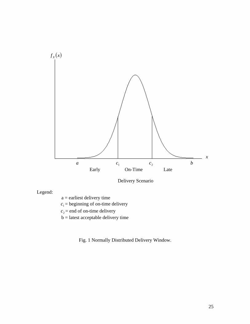
delivery process: reliability. They argue that modeling delivery reliability, e.g. variability, is the key to improving the delivery process. Within the delivery window, a delivery may be classified as early, on-time, or late. Figure 1 illustrates a delivery window for normally distributed delivery. Delivery lead time, X, is a random variable with probability density function ( )xf X . The on-time portion of the delivery window is defined by 12 cc − . Ideally, 012 =− cc . However, the extent to which may be measured in hours, days, or weeks depending on the industrial situation.

012 >− cc

<Insert Fig. 1 about here>

2.2 Model Development Consider a supply chain in operation over a time horizon of length T years, where a demand requirement for a single product of D units will be met with a constant delivery lot size Q. A single supplier provides a buyer with the delivery of a make-to-order product. Let X represent the delivery time for Q; the elapsed time from the receipt of an order by the supplier to the receipt of the delivery lot size by the buyer. Hence, the delivery time consists of the internal manufacturing lead-time(s) of the supplier, plus the external lead time associated with transporting the lot size from supplier to buyer. For a two-stage supply chain the expected penalty cost per period for untimely delivery, Y, is

(1) ( ) ( )dxxfcxKdxxfxcQHY X

b

cX

c

a∫∫ −+−=2

1

21 )()(

where Q = constant delivery lot size H = supplier’s inventory holding cost per unit per unit time K = penalty cost per time unit late (levied by the buyer). a, b, , = parameters defining the delivery window 1c 2c delivery lead time component at stage=iW ( )2,1=i = density function of delivery time X. ( )

21 WWX fxf += The individual lead time components at each stage of the supply chain are modeled using the normal distribution and independence between stages is assumed. Normality and independence among stages is often assumed in the literature (see for example Erlebacher and Singh, 1999; Tyworth and O’Neill, 1997). It is further assumed that delivery performance is stable enough so that the modal delivery time is within the on- time portion of the delivery window. For situations necessitating the need to truncate the normal density to prevent nonnegative delivery times or select other density functions defined for only positive values of the delivery time see Guiffrida (1999).

5

The penalty cost, K, is an opportunity cost due to lost production. Dion et al. (1991) reported that purchasing managers view the production disruptions caused by delivery stockouts to be more widespread and more costly than the lost sales that stockouts cause.

ence, K has been defined as an opportunity cost due to lost production as described by HFrame (1992), and Russell and Taylor (1998). Simplifying (1) and introducing ( )⋅φ and ( )⋅Φ as the standard normal density and umulative distribution functions respectively, yields the total expected penalty cost for

ally distributed delivery time

cnorm

( ) ( ) .1 22

211

1

⎥⎥⎦

⎤

⎢⎢⎣

⎡⎟⎟⎠

⎞⎜⎜⎝

⎛⎟⎟⎠

⎞⎜⎜⎝

⎛ −Φ−−−⎟⎟

⎠

⎞⎜⎜⎝

⎛ −+

⎥⎥⎦

⎤

⎢⎢⎣

⎡⎟⎟⎠

⎞⎜⎜⎝

⎛⎟⎟⎠

⎞⎜⎜⎝

⎛ −Φ−+⎟⎟

⎠

⎞⎜⎜⎝

⎛ −=

vc

cv

cvK

vc

cv

cvQHY

µµ

µφ

µµ

µφ (2)

an ill

e distribution. The ext section examines the dynamics of these three approaches on the expected penalty

ry distribution is normally distributed.

is

e

he potential problem associated with reducing the on-time portion of the elivery window, when no action is taken to alter the mean and variance of the delivery

roposition 1. For a fixed mean and variance, reducing the on-time portion of the window increases the expected penalty cost.

f. ith no loss of generality, let the on-time portion of the delivery window be defined such

that

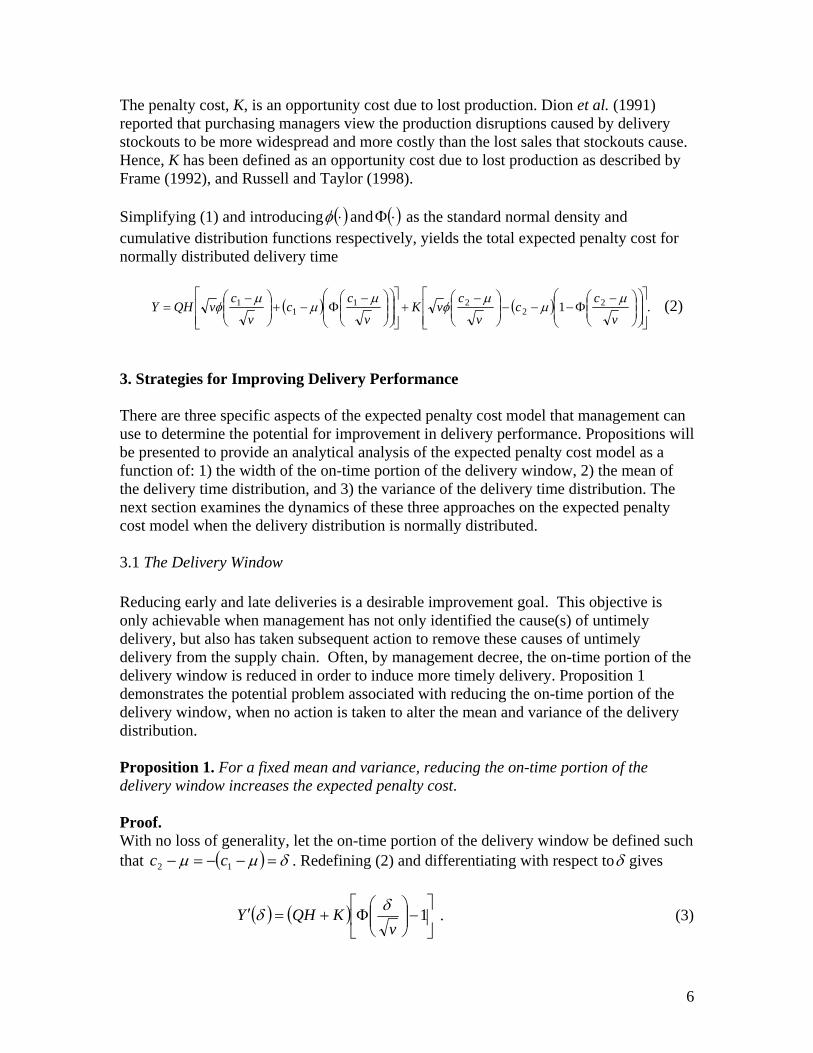
3. Strategies for Improving Delivery Performance

There are three specific aspects of the expected penalty cost model that management cuse to determine the potential for improvement in delivery performance. Propositions wbe presented to provide an analytical analysis of the expected penalty cost model as a function of: 1) the width of the on-time portion of the delivery window, 2) the mean of the delivery time distribution, and 3) the variance of the delivery timncost model when the delive 3.1 The Delivery Window Reducing early and late deliveries is a desirable improvement goal. This objectiveonly achievable when management has not only identified the cause(s) of untimely delivery, but also has taken subsequent action to remove these causes of untimely delivery from the supply chain. Often, by management decree, the on-time portion of thdelivery window is reduced in order to induce more timely delivery. Proposition 1 demonstrates tddistribution. Pdelivery ProoW

( ) δµµ =−−=− 12 cc . Redefining (2) and differentiating with respect toδ gives

( ) ( ) ⎥⎦

⎤⎢⎣

⎡−⎟⎟

⎠

⎞⎜⎜⎝

⎛Φ+=′ 1

vKQHY δδ . (3)

6

Examining (3), ( ) 0<′ δY for all 0≥δ . Hence, for a constant mean and variance, arbitrarily reducing the width of the on-time portion of delivery window will result in an

crease in the expected penalty cost.

r reducing the width of the on-time portion of the delivery window by

in For a constant mean and variance, the percentage increase in the expected penalty cost

αfo percent is

( ) ( )

( ) .100,

,,1×⎥⎦

⎤⎢⎣

⎡ −−=Ψ

vYvYvY

δδδα (4)

Remark 1. For 10 <<α , the maximum increase in the expected penalty cost for

ducing the width of the on-time portion of the delivery window is bounded by

re

( ) 11max − xxR

2exp 2

−<Ψx (5)

herew vx δ= and = Mill’s Ratio.

.2 Mean of the Delivery Distribution

very distribution when the delivery window and variability of delivery are held onstant.

the mean of the delivery distribution will decrease the total expected penalty cost when

xR 3 This section will outline an analysis of the expected penalty cost with respect to the mean of the delic Proposition 2. For a fixed delivery window and constant variance, reducing

( ) ( ).µµ lateearly YY ′>′

ess components of the xpected penalty cost with respect to the mean are, respectively

Proof. The first derivatives of the expected earliness and expected latene

( ) ⎥⎦

⎤⎢⎣

⎜⎝ vearly

⎡⎟⎟⎠

⎞⎜⎛ −

Φ−=′ cQHY µµ 1 and ( ) ⎥

⎦

⎤⎢⎣

⎡⎟⎟⎠

⎞⎜⎜⎝

⎛ −Φ−=′

vcKYlate

µµ 21 . (6)

n of the the total expected enalty cost when

Decreasing the mea delivery distribution leads to a decrease in

( ) 0<′ µY . This condition is achievable only when ( ) ( ).µµ lateearly YY ′>′ p Remark 1. For a fixed delivery window and constant variance, reducing the mean of the delivery distribution will increase the total expected penalty cost when

( ) ( ).µµ lateearly YY ′<′

7

Proof. Decreasing the mean of the delivery distribution leads to an increase in the total expected penalty cost when ( ) 0>′ µY . This condition is achievable only when

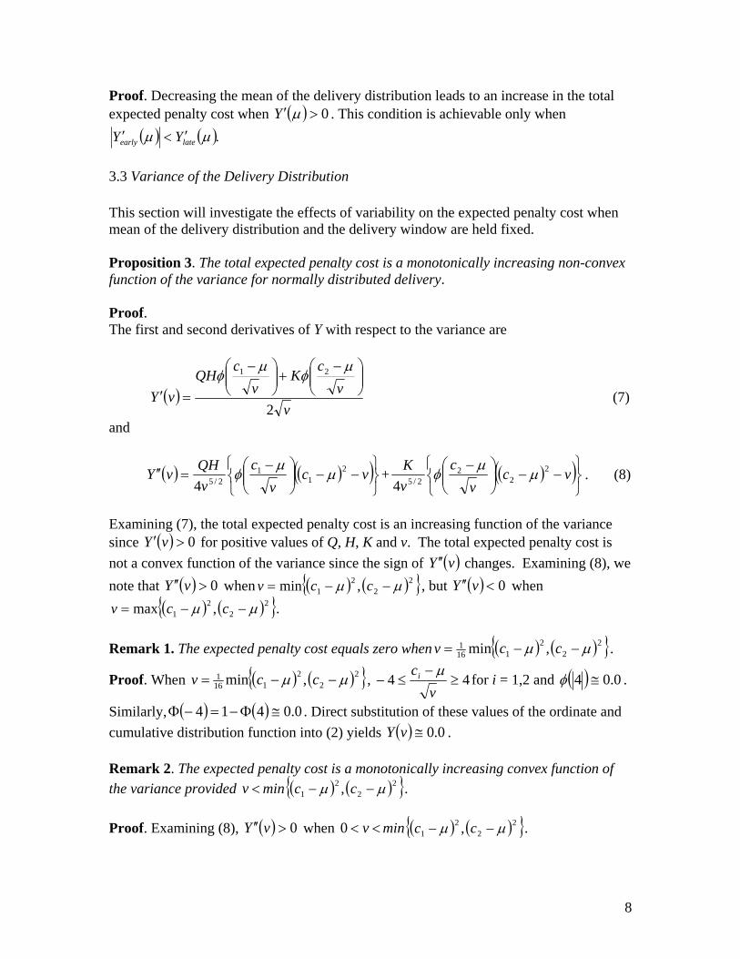
( ) ( ).µµ lateearly YY ′<′ 3.3 Variance of the Delivery Distribution This section will investigate the effects of variability on the expected penalty cost when mean of the delivery distribution and the delivery window are held fixed. Proposition 3. The total expected penalty cost is a monotonically increasing non-convex function of the variance for normally distributed delivery. Proof. The first and second derivatives of Y with respect to the variance are

( )v

vc

Kv

cQH

vY2

21⎟⎟⎠

⎞⎜⎜⎝

⎛ −+⎟⎟

⎠

⎞⎜⎜⎝

⎛ −

=′

µφ

µφ

(7)

and

( ) ( )( )⎭⎬⎫

⎩⎨⎧

−−⎟⎟⎠

⎞⎜⎜⎝

⎛ −=′′ vc

vc

vQHvY 2

11

2/54µ

µφ + ( )( )

⎭⎬⎫

⎩⎨⎧

−−⎟⎟⎠

⎞⎜⎜⎝

⎛ −vc

vc

vK 2

22

2/54µ

µφ . (8)

Examining (7), the total expected penalty cost is an increasing function of the variance since for positive values of Q, H, K and v. The total expected penalty cost is not a convex function of the variance since the sign of

( ) 0>′ vY( )vY ′′ changes. Examining (8), we

note that when( ) 0>′′ vY ( ) ( ) 22

21 ,min µµ −−= ccv , but ( ) 0<′′ vY when

( ) ( ) 22

21 ,max µµ −−= ccv .

Remark 1. The expected penalty cost equals zero when ( ) ( ) 2

22

1161 ,min µµ −−= ccv .

Proof. When ( ) ( ) 22

2116

1 ,min µµ −−= ccv , 44 ≥−

≤−v

ci µ for i = 1,2 and ( ) 0.04 ≅φ .

Similarly, . Direct substitution of these values of the ordinate and cumulative distribution function into (2) yields

( ) ( ) 0.0414 ≅Φ−=−Φ( ) 0.0≅vY .

Remark 2. The expected penalty cost is a monotonically increasing convex function of the variance provided min<v ( ) ( ) 2

22

1 , µµ −− cc . Proof. Examining (8), when ( ) 0>′′ vY << v0 min ( ) ( ) 2

22

1 , µµ −− cc .

8

3.4 Joint Optimization of the Expected Penalty Cost Based on the Mean and Variance of

elivery

l ea alty cost will be denoted by subscripts. he Hessian

D For notationa se derivatives of the expected pen

H matrix for ( )vY ,µT is defined as

⎢⎢⎢⎢⎢⎢⎢

⎣

⎡

⎪⎭

⎪⎬⎫

⎪⎩

⎪⎨⎧

⎟⎟⎠

⎞⎜⎜⎝

⎛ −⎟⎟⎠

⎞⎜⎜⎝

⎛ −+

⎪⎭

⎪⎬⎫

⎪⎩

⎪⎨⎧

⎟⎟⎠

⎞⎜⎜⎝

⎛ −⎟⎟⎠

⎞⎜⎜⎝

⎛ −

⎪⎭

⎪⎬⎫

⎪⎩

⎪⎨⎧

⎟⎟⎠

⎞⎜⎜⎝

⎛ −+

⎪⎭

⎪⎬⎫

⎪⎩

⎪⎨⎧

⎟⎟⎠

⎞⎜⎜⎝

⎛ −

=

vc

vcK

vc

vcQH

vc

vK

vc

vQH

Hµµ

φµµ

φ

µφµφ

2211

21

( )( ) ( )( )

⎥⎥⎥⎥⎥⎥⎥

⎦

⎤

⎪⎭

⎪⎬⎫

⎪⎩

⎪⎨⎧

−−⎟⎟⎠

⎞⎜⎜⎝

⎛ −+

⎪⎭

⎪⎬⎫

⎪⎩

⎪⎨⎧

−−⎟⎟⎠

⎞⎜⎜⎝

⎛ −

⎪⎭

⎪⎬⎫

⎪⎩

⎪⎨⎧

⎟⎟⎠

⎞⎜⎜⎝

⎛ −⎟⎟⎠

⎞⎜⎜⎝

⎛ −+

⎪⎭

⎪⎬⎫

⎪⎩

⎪⎨⎧

⎟⎟⎠

⎞⎜⎜⎝

⎛ −⎟⎟⎠

⎞⎜⎜⎝

⎛ −

vcv

cvKvc

vc

vQH

vc

vcK

vc

vcQH

22

22/5

21

12/5

2211

44µ

µφµ

µφ

µµφµµφ

.

The Hess ositive definite to satisfy the convexity uClearly,

ian must be p conditions for a minim m. 01 >= µµYH , however, the comp nature of licated ( )( ) ( )22 vvv YYYH µµµ −=

precludes a direct analysis

to determine if 0 . The convex lysi2 >H ity ana s can be mplified by introducing ( ) δµµ =−−=− 12 cc and analyzing ( )vY ,δsi .

a convex function of the width of the delivery

window and the variance of delivery when

Proposition 4. The expected penalty cost is

QHKv 2

KQH +>

δ .

roof. When the on-time portion of the delivery window is symmetric, the Hessian is

H =

P

( ) ( )

( ) ( ) ⎥⎥⎥⎥⎥⎥

⎦

⎤

⎢⎢⎢⎢⎢⎢

⎣

⎡

−⎟⎟⎠

⎞⎜⎜⎝

⎛+⎟⎟⎠

⎞⎜⎜⎝

⎛−

⎟⎟⎠

⎞⎜⎜⎝

⎛−⎟⎟⎠

⎞⎜⎜⎝

⎛+

vvv

KQHvv

QHK

vvQHK

vvKQH

22/52/3

2/32/1

42

2

δδφδφδ

δφδδφ

. (9)

rinciple minor is clearly positive. The second principle minor is positive

The first pprovided

QHKKQH

v 2+

>δ . (10)

Let

KQH

=η , then (10) isη

ηδ2

1+>

v. This constraint is illustrated for selected values of

η in Figure 2.

<Insert Fig. 2 about here>

9

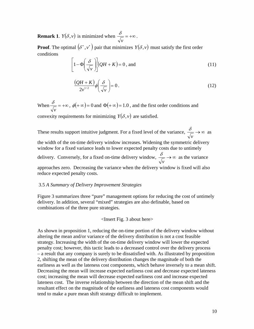
Remark 1. ( vY , )δ is minimized when +∞=vδ .

Proof. The optimal ( )∗∗ v,δ pair that minimizes ( )vY ,δ must satisfy the first order conditions

( ) 01 =+⎥⎦

⎤⎢⎣

⎡⎟⎟⎠

⎞⎜⎜⎝

⎛Φ− KQH

vδ , and (11)

( ) 02 2/1 =⎟⎟

⎠

⎞⎜⎜⎝

⎛+vv

KQH δφ . (12)

When +∞=vδ , ( ) 0=∞+φ and ( ) 0.1=∞+Φ , and the first order conditions and

convexity requirements for minimizing ( )vY ,δ are satisfied.

These results support intuitive judgment. For a fixed level of the variance, ∞→vδ as

the width of the on-time delivery window increases. Widening the symmetric delivery window for a fixed variance leads to lower expected penalty costs due to untimely

delivery. Conversely, for a fixed on-time delivery window, ∞→vδ as the variance

approaches zero. Decreasing the variance when the delivery window is fixed will also reduce expected penalty costs. 3.5 A Summary of Delivery Improvement Strategies Figure 3 summarizes three “pure” management options for reducing the cost of untimely delivery. In addition, several “mixed” strategies are also definable, based on combinations of the three pure strategies.

<Insert Fig. 3 about here> As shown in proposition 1, reducing the on-time portion of the delivery window without altering the mean and/or variance of the delivery distribution is not a cost feasible strategy. Increasing the width of the on-time delivery window will lower the expected penalty cost; however, this tactic leads to a decreased control over the delivery process – a result that any company is surely to be dissatisfied with. As illustrated by proposition 2, shifting the mean of the delivery distribution changes the magnitude of both the earliness as well as the lateness cost components, which behave inversely to a mean shift. Decreasing the mean will increase expected earliness cost and decrease expected lateness cost; increasing the mean will decrease expected earliness cost and increase expected lateness cost. The inverse relationship between the direction of the mean shift and the resultant effect on the magnitude of the earliness and lateness cost components would tend to make a pure mean shift strategy difficult to implement.

10

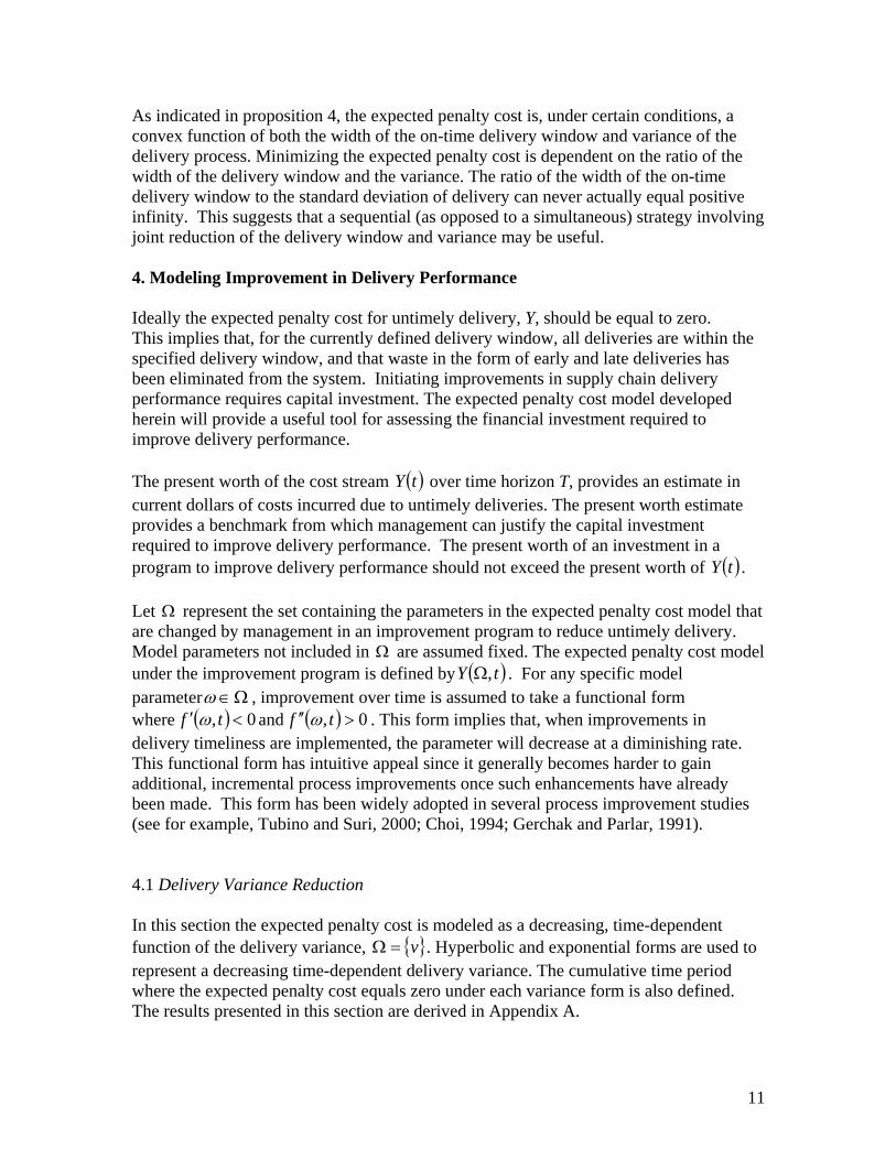
As indicated in proposition 4, the expected penalty cost is, under certain conditions, a convex function of both the width of the on-time delivery window and variance of the delivery process. Minimizing the expected penalty cost is dependent on the ratio of the width of the delivery window and the variance. The ratio of the width of the on-time delivery window to the standard deviation of delivery can never actually equal positive infinity. This suggests that a sequential (as opposed to a simultaneous) strategy involving joint reduction of the delivery window and variance may be useful. 4. Modeling Improvement in Delivery Performance Ideally the expected penalty cost for untimely delivery, Y, should be equal to zero. This implies that, for the currently defined delivery window, all deliveries are within the specified delivery window, and that waste in the form of early and late deliveries has been eliminated from the system. Initiating improvements in supply chain delivery performance requires capital investment. The expected penalty cost model developed herein will provide a useful tool for assessing the financial investment required to improve delivery performance. The present worth of the cost stream ( )tY over time horizon T, provides an estimate in current dollars of costs incurred due to untimely deliveries. The present worth estimate provides a benchmark from which management can justify the capital investment required to improve delivery performance. The present worth of an investment in a program to improve delivery performance should not exceed the present worth of ( )tY . Let Ω represent the set containing the parameters in the expected penalty cost model that are changed by management in an improvement program to reduce untimely delivery. Model parameters not included in Ω are assumed fixed. The expected penalty cost model under the improvement program is defined by ( )tY ,Ω . For any specific model parameter Ω∈ω , improvement over time is assumed to take a functional form where ( ) 0, <′ tf ω and ( ) 0, >′′ tf ω . This form implies that, when improvements in delivery timeliness are implemented, the parameter will decrease at a diminishing rate. This functional form has intuitive appeal since it generally becomes harder to gain additional, incremental process improvements once such enhancements have already been made. This form has been widely adopted in several process improvement studies (see for example, Tubino and Suri, 2000; Choi, 1994; Gerchak and Parlar, 1991). 4.1 Delivery Variance Reduction In this section the expected penalty cost is modeled as a decreasing, time-dependent function of the delivery variance, v=Ω . Hyperbolic and exponential forms are used to represent a decreasing time-dependent delivery variance. The cumulative time period where the expected penalty cost equals zero under each variance form is also defined. The results presented in this section are derived in Appendix A.

11

Hyperbolic Delivery Variance Reduction

Hyperbolic reduction in the variance of delivery is defined as ( ) tMtvf =, , where the parameter M represents the level of variance in the delivery distribution prior to the adoption of an improvement program to reduce delivery variance. The expected penalty cost under hyperbolic variance reduction is

( ) ( ) ( ) ( )( ) +⎥⎦

⎤⎢⎣

⎡Φ−+−= tzctk

tMQHtvY 11111exp2

, µπ

(13)

( ) ( ) ( )( )( )⎥⎦

⎤⎢⎣

⎡Φ−−−− tzctk

tMK 21221 1exp2

µπ

where: ( )

Mc

k ii 2

2

1µ−

= and ( ) ( )Mtctz ii µ−=1 for i = 1,2.

The cumulative time period when the expected penalty cost equals zero, , can be found by setting and solving for t. Let

∗t( ) 0, =tvf µµτ −−= 21 ,min cc . For hyperbolic

variance reduction 24⎟⎠⎞

⎜⎝⎛=∗

τMt .

Exponential Delivery Variance Reduction Exponential reduction in the variance of delivery is defined as ( ) rtPetvf −=, , where the parameters P and r represent the level of variance in the delivery distribution prior to the adoption of an improvement program to reduce delivery variance and the variance decay rate respectively. The expected penalty cost under exponential variance reduction is

( ) ( )( ) ( ) ( )( ) +⎥⎦

⎤⎢⎣

⎡Φ−++−= tzcekrtPQHtvY rt

1211221exp

2, µ

π (14)

( )( ) ( ) ( )( )( )⎥⎦

⎤⎢⎣

⎡Φ−−−+− tzcekrtPK rt

2222221 1exp

2µ

π

where: ( )P

ck i

i

2

2µ−

= and ( ) ( )Pectz

rt

ii µ−=2 for i = 1,2.

Under exponential variance reduction, the cumulative time period when the expected

penalty cost equals zero is ⎥⎥⎦

⎤

⎢⎢⎣

⎡⎟⎠

⎞⎜⎝

⎛−=∗

2

4ln1

Prt τ .

12

4.2 Delivery Window Reduction In this section the expected penalty cost is modeled as a decreasing function of the width of the on-time portion of the delivery window, µδ −==Ω ii c for i = 1,2. Hyperbolic and exponential forms are used to represent a decreasing on-time delivery window as a function of time. The results presented in this section are derived in Appendix B. Hyperbolic Delivery Window Reduction Hyperbolic reduction in the width of the on-time portion of the delivery window is

defined as ( )t

ctf i

iµ

δ−

=, for i = 1,2. The expected penalty cost under hyperbolic

delivery window reduction is

( ) +⎥⎥⎦

⎤

⎢⎢⎣

⎡⎟⎟⎠

⎞⎜⎜⎝

⎛Φ⎟⎠⎞

⎜⎝⎛+⎟⎟

⎠

⎞⎜⎜⎝

⎛−=

vttvtvQHtY 11

2

21

2exp

2, δδδ

πδ (15)

⎥⎥⎦

⎤

⎢⎢⎣

⎡⎟⎟⎠

⎞⎜⎜⎝

⎛⎟⎟⎠

⎞⎜⎜⎝

⎛Φ−⎟

⎠⎞

⎜⎝⎛−⎟⎟

⎠

⎞⎜⎜⎝

⎛−

vttvtvK 22

2

22 1

2exp

2δδδ

π.

Exponential Delivery Window Reduction Exponential reduction in the width of the on-time portion of the delivery window is defined for decay rate r as ( ) ( ) rt

ii ectf −−= µδ , for i = 1,2. The expected penalty cost under hyperbolic delivery window reduction is

( ) ( ) +⎥⎥⎦

⎤

⎢⎢⎣

⎡⎟⎟⎠

⎞⎜⎜⎝

⎛Φ+⎟⎟

⎠

⎞⎜⎜⎝

⎛−=

−−

−

ve

ev

evQHtYrt

rtrt

11

221

2exp

2,

δδ

δπ

δ (16)

( )⎥⎥⎦

⎤

⎢⎢⎣

⎡⎟⎟⎠

⎞⎜⎜⎝

⎛⎟⎟⎠

⎞⎜⎜⎝

⎛Φ−−⎟⎟

⎠

⎞⎜⎜⎝

⎛−

−−

−

vee

vevK

rtrt

rt2

2

222 12

exp2

δδ

δπ

.

4.3 Joint Reduction in Variance and Delivery Window In this section hyperbolic and exponential models are presented for joint reduction of the variance of delivery and the width of the on-time portion of the delivery window,

iv δ,=Ω for i = 1,2. Joint Hyperbolic Variance and Delivery Window Reduction An expression for joint hyperbolic reduction in the delivery variance and the width of the on-time portion of the delivery window is found by substituting the hyperbolic form into

13

(A-2) and (A-3). The expected penalty cost for joint hyperbolic reduction in delivery variance and width of the on-time portion of the delivery window is

( ) +⎥⎥⎦

⎤

⎢⎢⎣

⎡⎟⎟⎠

⎞⎜⎜⎝

⎛Φ⎟⎠⎞

⎜⎝⎛+⎟⎟

⎠

⎞⎜⎜⎝

⎛−=

MttMttMQHtvY 11

21

2exp

2,, δδδ

πδ (17)

⎥⎥⎦

⎤

⎢⎢⎣

⎡⎟⎟⎠

⎞⎜⎜⎝

⎛⎟⎟⎠

⎞⎜⎜⎝

⎛Φ−⎟

⎠⎞

⎜⎝⎛−⎟⎟

⎠

⎞⎜⎜⎝

⎛−

MttMttMK 22

22 1

2exp

2δδδ

π.

Joint Exponential Variance and Delivery Window Reduction An expression for joint exponential reduction in the delivery variance and the width of the on-time portion of the delivery window is found by substituting the exponential form into (A-4) and (A-5). The expected penalty cost for joint exponential reduction in delivery variance and width of the on-time portion of the delivery window is

( )( )

( )( )

+⎥⎥⎦

⎤

⎢⎢⎣

⎡⎟⎟⎠

⎞⎜⎜⎝

⎛Φ+

⎭⎬⎫

⎩⎨⎧ +−=

−−−

−

Pee

PtPrePQHtvY

rrttr

rrt 2/1

11

221

122

21

2exp

2,, δ

δδ

πδ (18)

( )

( )( )

⎥⎥⎦

⎤

⎢⎢⎣

⎡⎟⎟⎠

⎞⎜⎜⎝

⎛⎟⎟⎠

⎞⎜⎜⎝

⎛Φ−−

⎭⎬⎫

⎩⎨⎧ +−

−−−

−

Pee

PtPrePK

rrttr

rrt 2/2

21

222

122

21

12

exp2

δδ

δπ

where: = decay rate of variance, = decay rate of on-time window and 1r 2r µδ −= ii c for i = 1,2. 4.5 Financially Justifying Investment for Delivery Improvement The present worth of provides management with a benchmark for justifying capital investment for improving supply chain delivery performance. Under continuous compounding, the present worth of the continuous cost flow

( )tY

( )tY can be evaluated using Laplace transformations (Grubbström, 1967; Buck and Hill, 1975). The Laplace transformation maps the cost flow function that is continuous in the time domain to a present worth function continuous in the interest rate (s) domain. The Laplace transformation of the expected penalty cost for a continuous improvement program defined over a finite time horizon Tt ≤≤0 is

. (19) ( )[ ] ( ) dtetYtYL stT

−∫ Ω=Ω0

,,

An analysis of the present worth of ( )tY using (19) is presented for the case of time-dependent reduction in delivery variance, v=Ω . Expressions for ( )[ ]tvYL , under

14

hyperbolic and exponential forms of time-dependent variance reduction are derived in Appendix C.

5. Conclusions This paper addressed one aspect of supply chain planning by modeling delivery performance using a cost-based measure. A model has been presented that financially evaluates the effects of untimely delivery. The model provides a framework for modeling the continuous improvement of delivery performance with a serial supply chain. The model incorporates the time value of money into the evaluation process and provides a means for justifying the resources required for investing in a continuous improvement program for supplier delivery performance. The model has been demonstrated under hyperbolic and exponential functions of delivery variance. Other cases can be explored in a similar manner. There are several aspects of this research that could be expanded. An optimization model could be used to determine and allocate variance reduction throughout the component stages of the supply chain subject to an investment constraint. Second, other reproductive and non-reproductive density functions could be used to model the individual component times of the various stages in the supply chain. Lastly, the assumption of independence among the stages could be investigated.

15

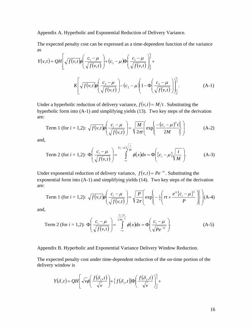
Appendix A. Hyperbolic and Exponential Reduction of Delivery Variance. The expected penalty cost can be expressed as a time-dependent function of the variance as

( ) ( )( )

( )( )

+⎥⎥⎦

⎤

⎢⎢⎣

⎡⎟⎟⎠

⎞⎜⎜⎝

⎛ −Φ−+⎟

⎟⎠

⎞⎜⎜⎝

⎛ −=

tvfcc

tvfctvfQHtvY

,,,, 1

11 µ

µµ

φ

( )( )

( )( ) ⎥

⎥⎦

⎤

⎢⎢⎣

⎡

⎟⎟

⎠

⎞

⎜⎜

⎝

⎛⎟⎟⎠

⎞⎜⎜⎝

⎛ −Φ−−−⎟

⎟⎠

⎞⎜⎜⎝

⎛ −

tvfcc

tvfctvfK

,1

,, 2

22 µ

µµ

φ . (A-1)

Under a hyperbolic reduction of delivery variance, ( ) tMtvf =, . Substituting the hyperbolic form into (A-1) and simplifying yields (13). Two key steps of the derivation are:

Term 1 (for i = 1,2): ( )( )

( )⎟⎟⎠

⎞⎜⎜⎝

⎛

⎪⎭

⎪⎬⎫

⎪⎩

⎪⎨⎧ −−

=⎟⎟⎠

⎞⎜⎜⎝

⎛ −M

tct

Mtvf

ctvf ii

2exp

2,,

2µπ

µφ (A-2)

and,

Term 2 (for i = 1,2): ( )

( ) ( )

∫−

∞−⎟⎟⎠

⎞⎜⎜⎝

⎛−Φ==⎟

⎟⎠

⎞⎜⎜⎝

⎛ −Φ

Mtc

ii

i

Mtcdxx

tvfc

µ

µφµ,

. (A-3)

Under exponential reduction of delivery variance, ( ) rtPetvf −=, . Substituting the exponential form into (A-1) and simplifying yields (14). Two key steps of the derivation are:

Term 1 (for i = 1,2): ( )( )

⎟⎟

⎠

⎞

⎜⎜

⎝

⎛

⎪⎭

⎪⎬⎫

⎪⎩

⎪⎨⎧

⎟⎟⎠

⎞⎜⎜⎝

⎛ −+−=⎟

⎟⎠

⎞⎜⎜⎝

⎛ −P

certP

tvfc

tvf irt

i2

21exp

2,,

µπ

µφ (A-4)

and,

Term 2 (for i = 1,2): ( )

( )∫−

−

∞−− ⎟⎟

⎠

⎞⎜⎜⎝

⎛ −Φ==⎟

⎟⎠

⎞⎜⎜⎝

⎛ −Φ

rti

Pe

c

rt

ii

Pe

cdxx

tvfc

µ

µφ

µ,

. (A-5)

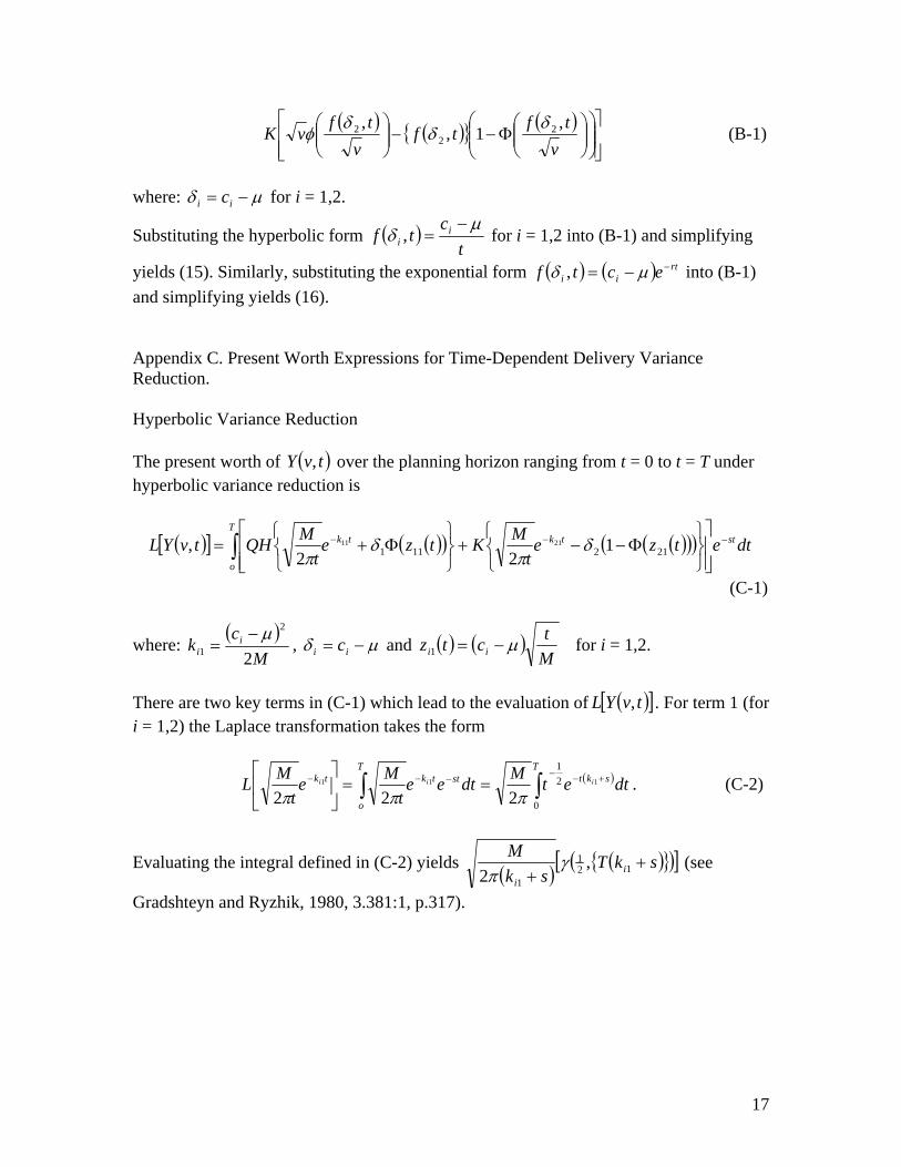
Appendix B. Hyperbolic and Exponential Variance Delivery Window Reduction. The expected penalty cost under time-dependent reduction of the on-time portion of the delivery window is

( ) ( ) ( ) ( )+⎥

⎦

⎤⎢⎣

⎡⎟⎟⎠

⎞⎜⎜⎝

⎛Φ+⎟⎟

⎠

⎞⎜⎜⎝

⎛=

vtftf

vtfvQHtY ,,,, 1

11 δ

δδ

φδ

16

( ) ( ) ( )⎥⎥⎦

⎤

⎢⎢⎣

⎡⎟⎟⎠

⎞⎜⎜⎝

⎛⎟⎟⎠

⎞⎜⎜⎝

⎛Φ−−⎟⎟

⎠

⎞⎜⎜⎝

⎛v

tftfv

tfvK ,1,, 22

2 δδ

δφ (B-1)

where: µδ −= ii c for i = 1,2.

Substituting the hyperbolic form ( )t

ctf i

iµ

δ−

=, for i = 1,2 into (B-1) and simplifying

yields (15). Similarly, substituting the exponential form ( ) ( ) rtii ectf −−= µδ , into (B-1)

and simplifying yields (16). Appendix C. Present Worth Expressions for Time-Dependent Delivery Variance Reduction. Hyperbolic Variance Reduction The present worth of over the planning horizon ranging from t = 0 to t = T under hyperbolic variance reduction is

( tvY , )

( )[ ] ( )( ) ( )( )( ) dtetzet

MKtzet

MQHtvYLT

o

sttktk∫ −−−

⎥⎥⎦

⎤

⎢⎢⎣

⎡

⎭⎬⎫

⎩⎨⎧

Φ−−+⎭⎬⎫

⎩⎨⎧

Φ+= 212111 122

, 2111 δπ

δπ

(C-1)

where: ( )

Mc

k ii 2

2

1µ−

= , µδ −= ii c and ( ) ( )Mtctz ii µ−=1 for i = 1,2.

There are two key terms in (C-1) which lead to the evaluation of ( )[ ]tvYL , . For term 1 (for i = 1,2) the Laplace transformation takes the form

( )dtetMdteet

Met

ML sktTT

o

sttktk iii +−−−−− ∫∫ ==⎥⎦

⎤⎢⎣

⎡111

0

21

222 πππ. (C-2)

Evaluating the integral defined in (C-2) yields ( ) ( ) ( )[ ]skTsk

Mi

i

++ 12

1

1

,2

γπ

(see

Gradshteyn and Ryzhik, 1980, 3.381:1, p.317).

17

For term 2 (for i = 1,2) the Laplace transform takes the form . The

Laplace identity

( )( ) dtetz stT

i−∫Φ

01

( )[ ] ( )[ xLxL s ]φ1=Φ for is used to evaluate term 2. To support the

nonnegative restriction of the identity let

0>x

( ) ( ) ( )duufduufzii zz

i ∫∫ −==Φ∞−

11

01 2

1 .

When i = 2, the Laplace identity can be applied directly. This yields 021 >z

( )( )[ ] ( )[ ]210

2121 1

21 zL

sdtetzL

Tst φ−=Φ− ∫ −

dtezs

dte stTT

st −− ∫∫ ⎟⎟⎠

⎞⎜⎜⎝

⎛−−=

0

221

0 2exp

21

21

π

( ) dteskts

dte stTT

st −− ∫∫ +−−=0

210

exp21

21

π

( )

⎭⎬⎫

⎩⎨⎧

++−−

−⎭⎬⎫

⎩⎨⎧ −

=−

21

21exp121

21

ksskt

sse st

π. (C-3)

When i = 1, and the nonnegative restriction in the Laplace identity can be maintained due to the symmetry defined by

012 <z( ) ( )1212 1 zz Φ−=−Φ . The result is identical

to that of (C-3) with used in place of . 11k 21k Using the key steps outlined above, the present worth of the expected penalty cost under hyperbolic delivery variance reduction is

( )[ ] ( ) ( )( ) ( )( )

+⎥⎥⎦

⎤

⎢⎢⎣

⎡⎟⎟⎠

⎞⎜⎜⎝

⎛⎟⎟⎠

⎞⎜⎜⎝

⎛+

−−

⎭⎬⎫

⎩⎨⎧ −

−+++

=+−−

111112

1

11

11121

21,

2,

kse

ssecskT

skMQHtvYL

skTsT

πµγ

π

( ) ( )( ) ( )

( )

⎥⎥⎦

⎤

⎢⎢⎣

⎡⎟⎟⎠

⎞⎜⎜⎝

⎛⎟⎟⎠

⎞⎜⎜⎝

⎛+

−−

⎭⎬⎫

⎩⎨⎧ −

−−++

+−−

212212

1

21

21121

21,

2 kse

ssecskT

skMK

skTsT

πµγ

π. (C-4)

Exponential Variance Reduction The present worth of over the planning horizon ranging from t = 0 to t = T under exponential variance reduction is

( tvY , )

18

( )[ ] ( )( ) ( )( ) +⎢⎢⎣

⎡

⎭⎬⎫

⎩⎨⎧

Φ++−= ∫T

rt tzekrtPQHtvYL0

1211221exp

2, δ

π

( )( ) ( )( )( ) dtetzekrtPK strt −

⎥⎥⎦

⎤

⎭⎬⎫

⎩⎨⎧

Φ−−+− 2222221 1exp

2δ

π (C-5)

where: ( )

Pc

k ii

2

2µ−

= , µδ −= ii c and ( ) ( )P

ectzrt

ii µ−=2 for i = 1,2.

There are two key terms in (C-5) which lead to the evaluation of ( )[ ]tvYL , . For term 1 (for i = 1,2) the Laplace transformation takes the form

( )( ) ( )( dteekrtPekrtPLT

o

strti

rti ∫ −+−=⎥

⎦

⎤⎢⎣

⎡+− 22

122

1 exp2

exp2 ππ

)

∫ −⎟⎠⎞

⎜⎝⎛ +−

=T

dtebrst rt

ieeP

0

2 2

2π (C-6)

where 2

22

ii

kb = . To evaluate (C-6) let , then rt

i ebu 2=rududt = and

r

i

t

bue

1

2⎟⎟⎠

⎞⎜⎜⎝

⎛= .

Under this substitution (C-6) can be written as

[ ] dueur

bPL ueb

b

rsr

s

i

rTi

i

−⎟⎠⎞

⎜⎝⎛ +−

⎟⎠⎞

⎜⎝⎛ +

∫⎥⎥⎥

⎦

⎤

⎢⎢⎢

⎣

⎡

=⋅2

2

232

1

2

2π

⎪⎭

⎪⎬⎫

⎪⎩

⎪⎨⎧

−⎥⎥⎥

⎦

⎤

⎢⎢⎢

⎣

⎡

= ∫ ∫∞ ∞

−⎟⎠⎞

⎜⎝⎛ +−

−⎟⎠⎞

⎜⎝⎛ +−

⎟⎠⎞

⎜⎝⎛ +

2 2

23

232

1

2

2i

rtib eb

urs

ursr

s

i dueudueur

bPπ

. (C-7)

Evaluating the integrals defined in (C-7) yields

[ ]⎭⎬⎫

⎩⎨⎧

⎟⎟⎠

⎞⎜⎜⎝

⎛

⎭⎬⎫

⎩⎨⎧ +−Γ−⎟⎟

⎠

⎞⎜⎜⎝

⎛

⎭⎬⎫

⎩⎨⎧ +−Γ

⎥⎥⎥

⎦

⎤

⎢⎢⎢

⎣

⎡

=⋅⎟⎠⎞

⎜⎝⎛ +

rTii

rs

i ebrsb

rs

rbPL 22

21

2 ,21,

21

2π (C-8)

(see Gradshteyn and Ryzhik, 1980, 3.381:3, p.317). The structure of the second term in (C-5) is similar to term 2 of the hyperbolic case and it follows directly from the steps outlined in (C-3) that for i = 1, 2

19

( )( )[ ] ( )[ ]20

221 1

21

i

Tst

i zLs

dtetzL φ−=Φ− ∫ −

( )∫ −−

−−⎭⎬⎫

⎩⎨⎧ −

=T

strti

st

dteebss

e

02exp

21

21

π. (C-9)

The integral in (C-9) can be evaluating using the substitutions defined in the evaluation of (C-6). This yields

[ ]⎭⎬⎫

⎩⎨⎧

⎟⎟⎠

⎞⎜⎜⎝

⎛

⎭⎬⎫

⎩⎨⎧ +−Γ−⎟⎟

⎠

⎞⎜⎜⎝

⎛

⎭⎬⎫

⎩⎨⎧ +−Γ

⎥⎥⎥

⎦

⎤

⎢⎢⎢

⎣

⎡

−⎭⎬⎫

⎩⎨⎧ −

=⋅⎟⎠⎞

⎜⎝⎛

−rT

ii

rs

isT

ebrsb

rs

rsb

seL 22

2 ,21,

21

221

π. (C-10)

Using the key steps outlined above, the present worth of the expected penalty cost under exponential delivery variance reduction is

( )[ ] +⎭⎬⎫

⎩⎨⎧

⎟⎟⎠

⎞⎜⎜⎝

⎛

⎭⎬⎫

⎩⎨⎧ +−Γ−⎟⎟

⎠

⎞⎜⎜⎝

⎛

⎭⎬⎫

⎩⎨⎧ +−Γ

⎥⎥⎥

⎦

⎤

⎢⎢⎢

⎣

⎡

⎢⎣

⎡=

⎟⎠⎞

⎜⎝⎛ +

rTrs

ebrsb

rs

rbPQHtvYL 1212

21

12 ,21,

21

2,

π

( )⎥⎥⎥⎥

⎦

⎤

⎟⎟⎟⎟

⎠

⎞

⎜⎜⎜⎜

⎝

⎛

⎭⎬⎫

⎩⎨⎧

⎟⎟⎠

⎞⎜⎜⎝

⎛

⎭⎬⎫

⎩⎨⎧ +−Γ−⎟⎟

⎠

⎞⎜⎜⎝

⎛

⎭⎬⎫

⎩⎨⎧ +−Γ

⎥⎥⎥

⎦

⎤

⎢⎢⎢

⎣

⎡

−⎭⎬⎫

⎩⎨⎧ −

−⎟⎠⎞

⎜⎝⎛

−rT

rs

sT

ebrsb

rs

rsb

sec 1212

121 ,

21,

21

221

πµ +

−⎭⎬⎫

⎩⎨⎧

⎟⎟⎠

⎞⎜⎜⎝

⎛

⎭⎬⎫

⎩⎨⎧ +−Γ−⎟⎟

⎠

⎞⎜⎜⎝

⎛

⎭⎬⎫

⎩⎨⎧ +−Γ

⎥⎥⎥

⎦

⎤

⎢⎢⎢

⎣

⎡

⎢⎣

⎡⎟⎠⎞

⎜⎝⎛ +

rTrs

ebrsb

rs

rbPK 2222

21

22 ,21,

21

2π

( )⎥⎥⎥⎥

⎦

⎤

⎟⎟⎟⎟

⎠

⎞

⎜⎜⎜⎜

⎝

⎛

⎭⎬⎫

⎩⎨⎧

⎟⎟⎠

⎞⎜⎜⎝

⎛

⎭⎬⎫

⎩⎨⎧ +−Γ−⎟⎟

⎠

⎞⎜⎜⎝

⎛

⎭⎬⎫

⎩⎨⎧ +−Γ

⎥⎥⎥

⎦

⎤

⎢⎢⎢

⎣

⎡

−⎭⎬⎫

⎩⎨⎧ −

−⎟⎠⎞

⎜⎝⎛

−rT

rs

sT

ebrsb

rs

rsb

sec 2222

222 ,

21,

21

221

πµ . (C-11)

20

References Ballou, R. H., Gilbert, S. M., Mukherjee, A., 2000. New managerial challenges from supply chain opportunities. Industrial Marketing Management, 29, 7-18. Blackhurst, J., Wu, T., O’Grady, P., 2004. Network-based approach to modeling uncertainty in a supply chain. International Journal of Production Research, 42(8), 1639- 1658. Buck, J. R., Hill, T. W., 1975. Additions to the Laplace transform methodology for economic analysis. The Engineering Economist, 20(3), 197-208. Burt, D. N., 1989. Managing suppliers up to speed. Harvard Business Review, July- August, 127-135. Chase, R. B., Aquilano, N. J., Jacobs, F. R., 1998. Production operations management, manufacturing and services, 8th Edition, Irwin/McGraw Hill, Boston. Carr, A., Pearson, J., 1999. Strategically managed buyer-supplier relationships and performance outcomes. Journal of Operations Management, 17(5), 497-519. Choi, J-W., 1994. Investment in the reduction of uncertainties in just-in-time purchasing systems. Naval Research Logistics, 41, 257-272. Cooper, M. C., Lambert, D. M., Pagh, J. D., 1997. Supply chain management: more than a new name for logistics, International Journal of Logistics Management, 8(1), 1-14. Corbett, L. M., 1992. Delivery windows – a new way on improving manufacturing flexibility and on-time delivery performance. Production and Inventory Management, 33(3), 74-79. Davis, T., 1993. Effective supply chain management. Sloan Management Review, 38(1), 35-46. Dion. P. A., Hasey, L. M., Dorin, P. C., Lundkin, J., 1991. Consequences of inventory stockouts. Industrial Marketing Management, 20(2), 23-27. Ellram, L. M., 2002. Strategic cost management in the supply chain: a purchasing and supply management perspective. CAPS Research. Erlebacher, S. J., Singh, M. R., 1999. Optimal variance structures and performance improvement of synchronous assembly lines. Operations Research, 47(4), 601-618.

21

Fawcett, S. E., Birou, L. M., 1993. Just-in-time sourcing techniques: current state of adoption and performance benefits. Production and Inventory Management Journal, 34(1), 18-24. Frame, P., 1992. Saturn to fine suppliers $500/minute for delays. Automotive News, December, 21, 36. Gerchak, Y., Parlar, M., 1991. Investing in reducing lead-time randomness in continuous review inventory models. Engineering Costs and Production Economics, 21(2), 191-197. Guiffrida, A. L., 1999. A cost-based model for evaluating vendor delivery performance. MS thesis, Department of Industrial Engineering, State University of New York at Buffalo. Gunasekaran, A. C., Patel, C., McGaughey, R. E., 2004. A framework for supply chain performance measurement. International Journal of Production Economics, 87(3), 333-347. Gunasekaran, A. C., Patel, C., Tirtiroglu, E., 2001. Performance measures and metrics in a supply chain environment. International Journal of Operations and Production Management, 21(1/2), 71-87. Gradshteyn, I. S., Ryzhik. I. M., 1980. Tables of integrals, series, and products. Academic Press, New York. Grout, J. R., 1996. A model of incentive contracts for just-in-time delivery. European Journal of Operational Research, 96, 139-147. Grubbström, R. W., 1967. On the application of the Laplace transform to certain economic problems. Management Science, 13(7), 558-567. Hadavi, K. C., 1996. Why do we miss delivery dates? Industrial Management, 38(5), 1-4. Jaruphongsa, W., Centinkaya, S., Lee, C-H., 2004. Warehouse space capacity and delivery time window considerations in dynamic lot-sizing for a simple supply chain. International Journal of Production Economics, 92(2), 169-180. Johnson, M. E., Davis, T., 1998. Improving supply chain performance by using order fulfillment metrics. National Productivity Review, 17(3), 3-16. Lalonde, B. J., Pohlen, T. L., 1996. Issues in supply chain costing. International Journal of Logistics Management, 7(1), 1-12.

22

Lancioni, R. A., 2000. New developments in supply chain management for the millennium. Industrial Marketing Management, 29, 1-6. Lee, C-H., Centinkaya, S., Wagelmans, A. P. M., 2001. A dynamic lot-sizing model with demand time windows. Management Science, 47(10), 1384-1395. Lockamy, A., McCormack, K., 2004. Linking SCOR planning practices to supply chain performance. International Journal of Operations and Production Management, 24(12), 1192-1218. Lockamy, A., Spencer, M. S., 1998. Performance measurement in a theory of constraints environment. International Journal of Production Research, 36(8), 2045-2060. Monczka, R. M., Morgan, J. P., 1994. Today’s measures just don’t make it. Purchasing, 116(6), 46-50. New, C. C., Sweeney, T. M., 1984. Delivery performance and throughput efficiency in UK manufacturing. International Journal of Physical Distribution and Materials Management, 14(7), 3-48. Russell, R., Taylor, B., 1998. Operations Management: Focusing on Quality and Competitiveness. Prentice-Hall. Sabri, E. H., Beamon, B. M., 2000. A multi-objective approach to simultaneous strategic and operational planning in supply chain design. Omega, 28(5), 581-590. Schneiderman, A. M., 1996. Metrics for the order fulfillment process (part 1). Journal of Cost Management, 10(2), 30-42. Tubino, F., Suri, R., 2000. What kind of “numbers” can a company expect after implementing quick response manufacturing?, Quick Response Manufacturing 2000 Conference Proceedings, R. Suri (Ed.), Society of Manufacturing Engineers Press, Dearbon, MI, 2000, 943-972. Tyworth, J. E., O’Neill, L., 1997. Robustness of the normal approximation of lead- time demand in a distribution setting, Naval Research Logistics, 44, 165-186. Van Hoek, R. I., 1998. Measuring the unmeasureable – measuring and improving performance in the supply chain, Supply Chain Management, 3(4), 187-192. Vachon, S., Klassen, R. D., 2002. An exploratory investigation of the effects of supply chain complexity on delivery performance. IEEE Transactions on Engineering Management, 49(2), 218-230.

23

Verma, R., Pullman, M. E., 1998. An analysis of the supplier certification process. Omega, International Journal of Management Science, 26(6), 739-750. Walker, T. W., Alber, K. L., 1999. Understanding supply chain management. APICS- the Performance Advantage, January 38-43.

24

( )xf X

x a b 1c 2c Early On-Time Late Delivery Scenario Legend: a = earliest delivery time = beginning of on-time delivery 1c = end of on-time delivery 2c b = latest acceptable delivery time

Fig. 1 Normally Distributed Delivery Window.

25

1.4

1.2

1.0 η

vδ

0.25 0.5 1.0 2.0 4.0 Legend:

K

QH=η

Q = delivery lot size H = inventory holding per unit per unit time K = production stoppage cost δ = width of on-time portion of delivery window v = variance of delivery distribution

Fig. 2. The Ratio of Delivery Window Width and Delivery Variance as a Function of Early and Late Delivery Cost.

26

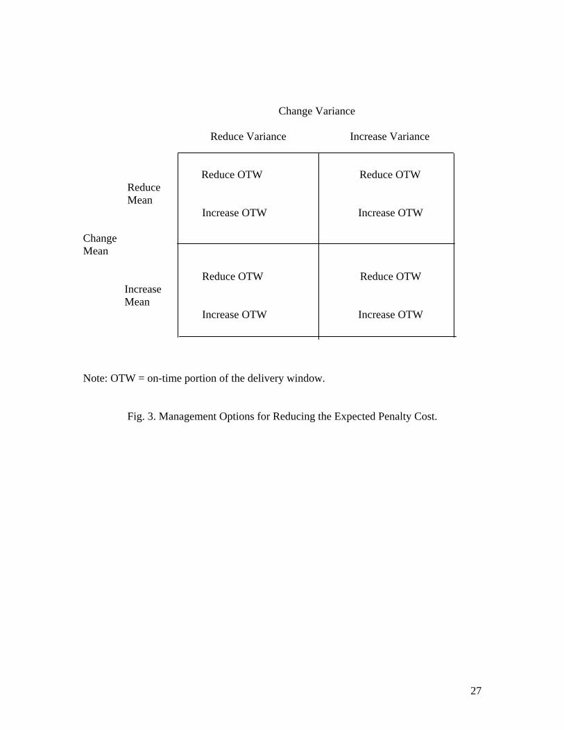
Change Variance Reduce Variance Increase Variance Reduce OTW Reduce OTW Reduce Mean Increase OTW Increase OTW Change Mean Reduce OTW Reduce OTW Increase Mean Increase OTW Increase OTW Note: OTW = on-time portion of the delivery window.

Fig. 3. Management Options for Reducing the Expected Penalty Cost.

27