cost assessment for pr19: a consultation on … cost modelling trust in water. ... (pr19) for water...

www.ofwat.gov.uk

March 2018

Cost assessment for PR19: a consultation oneconometric cost modelling

Trust in water

Cost assessment for PR19: a consultation on econometric cost modelling

1

About this document

This document is a consultation on a range of econometric cost assessment models for

the 2019 price review (PR19) for water and wastewater companies in England and

Wales.

In December 2017 we published our methodology for PR19. We set out in our

methodology that an important element of our approach to cost assessment is the

development of econometric models. We use econometric models to carry out a

comparative efficiency assessment of the sector. This assessment plays a key role in

setting an efficient level of expenditure for water companies.

This consultation includes models proposed by us as well as models proposed by water

companies.

We are seeking the views of all interested parties and welcome feedback on the

proposed models by 4 May 2018. Responses to this consultation will help us to select a

set of robust cost models for our efficiency assessment in PR19.

Alongside this consultation we publish a report we have commissioned from CEPA Ltd

on econometric models for wholesale water and wastewater controls. This consultation

includes some of the models proposed by CEPA.

https://www.ofwat.gov.uk/regulated-companies/price-review/2019-price-review-final-methodology/


2

Contents

1. Introduction ........................................................................................................................... 4

2. Approach to modelling .......................................................................................................... 8

3. Cost models for wholesale water activities .......................................................................... 13

4. Cost models for wholesale wastewater activities ................................................................. 18

5. Modelling for the residential retail controls .......................................................................... 22

6. Modelling for enhancement expenditure ............................................................................. 26


3

Responding to this consultation

The closing date for the consultation is 4 May 2018. Please email responses to

[email protected]. We will publish responses to this consultation on

our website at www.ofwat.gov.uk, unless you indicate that you would like your response

to remain unpublished.

We published a response spreadsheet, which allows respondents to rate and

provide a comment on each model in this consultation.

We would also welcome views on the level of aggregation for cost benchmarking,

in light of modelling results.

Information provided in response to this consultation, including personal information,

may be published or disclosed in accordance with access to information legislation –

primarily the Freedom of Information Act 2000 (FoIA), the Data Protection Act 1998 and

the Environmental Information Regulations 2004.

If you would like the information that you have provided to be treated as confidential,

please be aware that, under the FoIA, there is a statutory ‘Code of Practice’ with which

public authorities must comply and which deals, among other things, with obligations of

confidence. In view of this, it would be helpful if you could explain to us why you regard

the information you have provided as confidential. If we receive a request for disclosure

of the information we will take full account of your explanation, but we cannot give an

assurance that we can maintain confidentiality in all circumstances. An automatic

confidentiality disclaimer generated by your IT system will not, of itself, be regarded as

binding on Ofwat.

At a minimum, we would expect to publish the name of all organisations that provide a

written response, even where there are legitimate reasons that the contents of those

written responses remain confidential.

mailto:[email protected]

http://www.ofwat.gov.uk/


4

1. Introduction

Background

Cost assessment is the setting of an efficient baseline for totex (that is, total expenditure

of companies including both capital and operational expenditure) for each company for

the price control period.

In December 2017 we published Delivering W2020: Our final methodology for the 2019

price review. In chapter 9, securing cost efficiency, we discussed our approach to cost

assessment.

An important element of our approach to cost assessment is the use of comparative

assessment to identify companies that are efficient. The efficient companies provide

important information when setting efficient cost baselines for the sector.

Our main tool to carry out the comparative assessment is econometric modelling.

In PR19 we will set up to six different controls for the larger water companies1 in England

and Wales. The controls are

Water resources

Water network plus

Wastewater network plus

Bioresources

Residential retail

Business retail (where appropriate)

We said that for all controls, except the business retail controls2, we will develop

econometric models as a tool to assess cost efficiency.

Our econometric models will play an important role in our initial assessment of business

plans, and later, in setting efficient cost allowances in draft and final determinations.

Where appropriate we will incorporate information from other sectors on levels of

efficiency. A recent report by KPMG has found potential for significant efficiency gains

from the recent introduction of the totex and outcomes framework.3 A report by PWC

1 By which we mean companies holding appointments as water and/or sewerage undertakers. 2 The business retail controls will apply to only to companies whose areas are wholly or mainly in Wales, and those water companies whose areas are wholly or mainly in England who have not exited the business retail market by the time we set price controls. 3 See https://www.ofwat.gov.uk/wp-content/uploads/2018/03/Ofwat-totex-efficiency_workshop-pack_FINAL.pdf. The full report is due to be published in April 2018.

https://www.ofwat.gov.uk/publication/delivering-water-2020-final-methodology-2019-price-review/

https://www.ofwat.gov.uk/publication/delivering-water-2020-final-methodology-2019-price-review/

https://www.ofwat.gov.uk/wp-content/uploads/2018/03/Ofwat-totex-efficiency_workshop-pack_FINAL.pdf

https://www.ofwat.gov.uk/regulated-companies/vulnerability/debt-management-and-other-retail-costs-research-and-recommendations/




5

found significant scope to improve cost performance in bad debt and retail costs.4 In

PR19, we expect company business plans to show a step change in efficiency, relative

to past periods.

Purpose of this consultation

Developing good econometric models is a challenging task. It requires a deep

understanding of the sector – for example, of the factors that drive water companies’

costs – and expert data analysis and modelling skills.

During 2016 and 2017, we have been working with stakeholders, through our cost

assessment working group, to develop and refine our data and tools for cost

assessment. In July 2017, companies submitted data tables with cost, and relevant non-

cost information (eg “cost driver” information) on their wholesale water and wastewater

services in the preceding six years, 2011-12 to 2016-17. This data has been subject to

extensive quality assurance. Based on this data submission, and information from the

annual performance reports, we have been developing econometric cost models for

PR19.

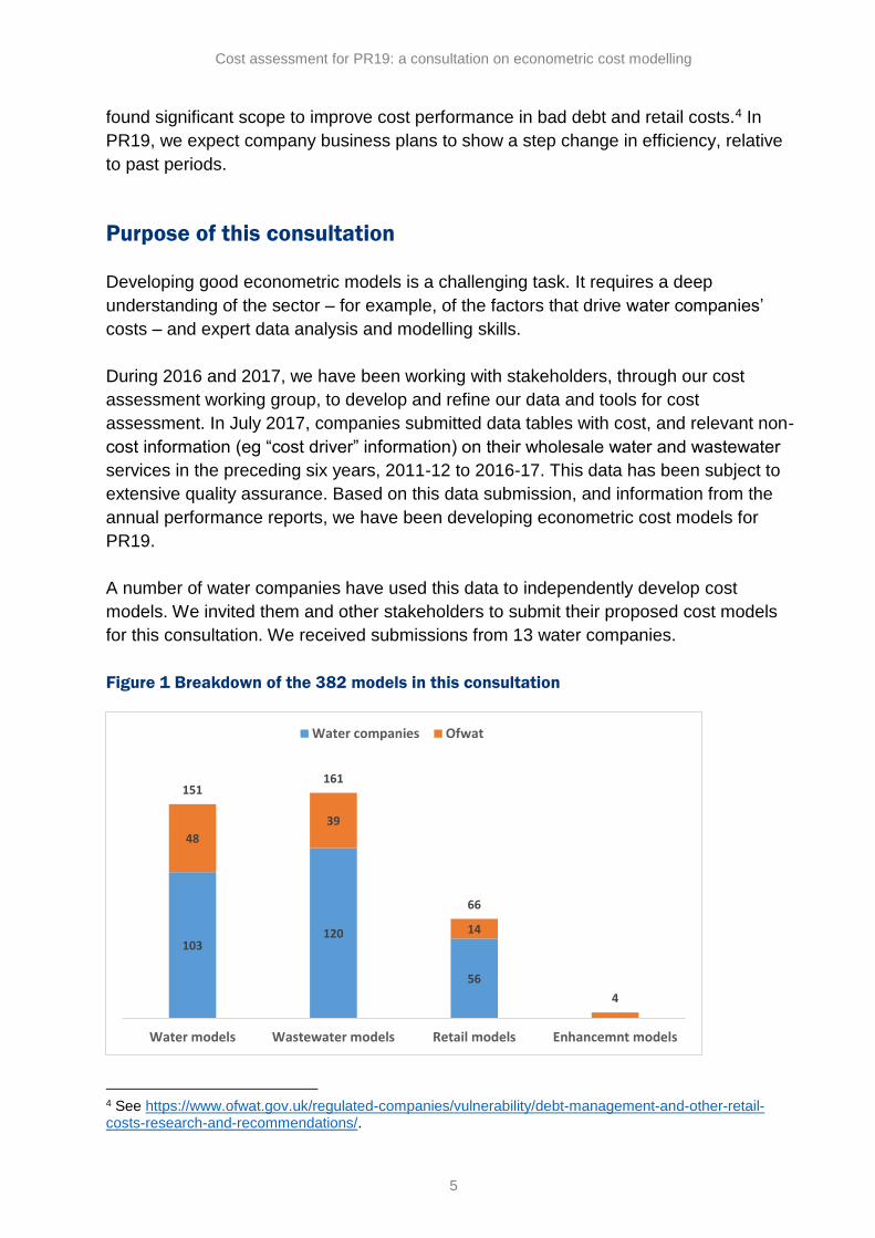
A number of water companies have used this data to independently develop cost

models. We invited them and other stakeholders to submit their proposed cost models

for this consultation. We received submissions from 13 water companies.

Figure 1 Breakdown of the 382 models in this consultation

4 See https://www.ofwat.gov.uk/regulated-companies/vulnerability/debt-management-and-other-retail-costs-research-and-recommendations/.

103120

56

48

39

14

151161

66

4

Water models Wastewater models Retail models Enhancemnt models

Water companies Ofwat




6

The purpose of this consultation is to draw on the knowledge and expertise of a wide set

of stakeholders. It brings together a large set of econometric cost models developed for

the various PR19 controls by us and, independently, by 13 water companies. The

consultation provides an opportunity for stakeholders to submit feedback on these

models.

The large pool of models and the stakeholder feedback will, in turn, help us select high

quality models for cost assessment. A high quality set of cost efficiency models is in the

interest of stakeholders and customers. The success of our models can have material

implications on customers’ bills. The higher the quality of our models, the more

confidence we can have in setting a stretching and appropriate efficiency challenge for

companies.

High quality models which reflect the underlying relationships of the business are also in

the interest of water companies, as they will be able to use them to scrutinise the

efficiency of their operation on an ongoing basis – not only for the purpose of price

controls.

Selection of models for PR19

Our final set of cost models for PR19 will be informed by responses to our consultation.

The final set of models need not be a subset of the models consulted on here. The final

set could include models that were developed based on further analysis and insight

following this consultation.

We will also re-assess the models in light of the 2017-18 data submission, due in July

2018, and data submitted in company business plans. This means that we will not

publish final cost models before companies submit their business plans on 3 September.

There have been a number of late revisions to the data, which have not yet been

incorporated to our data, and are therefore not reflected in modelling results. Once we

incorporate these revisions, the performance of some of the models may be affected. We

do not expect that the revisions will have a substantive impact on the models, but it will

impact on the exact value of the estimated coefficients.

Good quality data is critical to the development of effective cost assessment models. We

have written to companies to emphasise the importance of good data quality and that we

will take this into account in our assessment of business plans.


7

We remind companies that we do not consider that publication of our final cost models is

an essential input to development of company business plans – companies should focus

on developing efficient business plans that deliver for their customers. Companies’

business plans should not be driven by regulatory models of cost assessment.


8

2. Approach to modelling

We have developed and tested multiple models. Our emphasis is to develop models that

are consistent with engineering, operational and economic understanding of cost drivers.

We aim to develop models that are sensibly simple (without pursuing simplicity for its

own sake). We aim to capture only the main cost drivers in each model, to allow for a

robust and stable estimation of the underlying relationship. The models that we present

in this consultation are simpler and more intuitive than the models at PR14. None of the

coefficients has an unintuitive sign.

Our approach has taken into account learnings from PR14, industry feedback, and the

Competition and Markets Authority (CMA) reference on Bristol Water’s PR14 price

controls.

We have engaged CEPA to support us in the development of econometric models for the

wholesale controls. Their report and recommendations are published alongside this

consultation.

Model development and assessment criteria

Our approach to model development and assessment is as follows:

1. Use engineering, operational and economic understanding to specify an

econometric model, and form expectations about the relationship between cost

and cost drivers in the model.

2. Assess whether the estimated coefficients are of the right sign and of plausible

magnitude.

3. Consider if the estimated coefficients are robust. For example, are they stable

and consistent across different specifications? Are the estimated coefficients

statistically significant?

4. Assess the consequences of cost drivers under management controls, in

particular, the risk of any perverse incentive.

5. Consider the statistical validity of the model more widely – does the model

perform well in terms of statistical tests and diagnostics?

6. Consider the appropriate estimation method.

We discuss each in turn.


9

Models consistent with engineering, operational and economic rationale

Our emphasis is to develop models that make sense, with cost drivers that adhere to

engineering, operational or economic rationale.

The first step was to consider which factors drive costs at each area of modelling. The

models should include at least one scale (also called output or volume) driver and other

primary cost drivers. We generally avoid using highly correlated variables. This can

contribute to the risk of forecasting inaccuracy.

Estimated coefficients of the right sign and of plausible magnitude

After specifying a model for estimation, we use actual data from the water companies to

estimate the relationship. This relationship is provided by the estimated coefficients.

The estimated coefficients are the most important parameters to examine as we assess

econometric models. We check that the sign of the coefficient aligns with expectations,

and that its magnitude is plausible.5 These two checks are important as they assess

modelling results against a set of pre-conceived expectations. As such, they are not

dependent entirely on the data at hand. Considering these expectations guards against

including variables that appear to be related (statistically) but there is no clear reason for

their inclusion.

Estimated coefficients that are robust

We would then want to see that the relationship estimated by our model is robust. That

is, that the estimated coefficients are robust to changes in the sample and stable across

a range of model specifications.6 We will also want to check the statistical significance of

the estimated coefficients, that is, the degree of confidence that we have in their value,

based on the data at hand.

We do not consider that the common thresholds of statistical significance (eg 95%

significance) need to be strictly followed for our model selection. The size of the sample

has a large effect on statistical significance. With a relatively small sample we are careful

not to dismiss mechanistically variables that are not strictly statistically significant, so

long as the significance is still reasonable and the estimation seems robust.

These very high thresholds are common in academic literature, where they may be used

as an informal pre-requisite for publication. In commercial and regulatory application,

5 A precise magnitude is difficult to anticipate and can be subject to judgement and error, as variables often pick up the effect of other factors. 6 We would expect stability of an estimated coefficient as long as alternative models include the removal or addition of explanatory variable that are uncorrelated with the variable in question.


10

results that are not statistically significant are frequently used. Variables with lower

statistical significance can make a valid contribution to the model.

Nevertheless, most of the estimated coefficients in our models are statistically significant.

One more point on statistical significance. The fact that a variable is statistically

significant does not mean that the variable is important in the context of the model. That

is, statistical significance does not imply economic significance – the variables’ impact on

companies’ costs may be quite immaterial. In a small sample we may need to trade off

statistical significance with economic significance given that we cannot accommodate

many explanatory factors in the models. It may be appropriate to exclude a statistically

significant variable if it is not important for the purpose of predicting costs and setting

efficient baselines. Excluding such variable could help improve the estimation of other

variables in the model.

Cost drivers under management control

A model that includes explanatory factors that are under management control can

present issues that need to be considered.

From an estimation point of view the concern is termed ‘endogeneity’. A factor that is

under management control may reflect efficiency (management). If we regard at least

part of the residual in the model to be related to efficiency, it opens the possibility that

such factor is correlated with the residual, ie is endogenous, thus creating bias. The bias

will impact both the estimated coefficients and the error term. This can distort the

model’s forecasts, and the estimation of relative efficiencies, which are based on the

error.

From a regulatory point of view there is a potential concern that including factors that are

under management control in the model could send the wrong signal or create a

perverse incentive for the regulated companies. For example, the volume of water

abstracted is to some extent under management control. Management can reduce

leakage, promote demand side efficiency etc. A model that uses the volume of water

abstracted to explain variation in costs due to scale, will have a positive coefficient and

may be deemed to provide a perverse incentive – for two otherwise identical companies,

the model will imply higher costs for the company that is less water efficient (and

therefore abstracts more water).

We note that our approach of setting independent cost baselines for companies

mitigates the concern of perverse incentive (although not the concern over bias). In the

example above, if our baselines are based on our view of an efficient level of water

abstraction, a company would not be ‘rewarded’ for inefficient abstraction.


11

Most cost drivers are, to some degree, under management control, particularly in the

longer term. It is important to assess the degree of management control, the potential

materiality of bias and the risk presented by any perverse incentive. There may well be a

case for keeping factors under management control in the model, as replacing them with

alternative cost drivers may present a greater risk of inadequately reflecting the

underlying cost drivers.

Statistical validity of our model

While the estimated coefficients are the most important parameters when assessing

models, an econometric model needs to have some statistical validity.

When estimating an econometric model, we obtain a range of model diagnostics and

statistical tests. These are used to assess the model specification. Comparison of these

diagnostics across similar specifications can be useful, and they can provide useful

guidance as we develop models, but they should not alone drive our model selection.

The Reset test (described in the appendix) is used to assess whether a model with

quadratic terms is appropriate. The inclusion of a quadratic term, or an interaction term,

allows for a company specific relationship between the cost and the cost driver. A failure

of the reset test should prompt a search for a more flexible specification, but need not in

itself be grounds for dismissing a model.

None of these statistical diagnostics provides a mechanistic rule for the rejection or

acceptance of models. Our focus has not been on finding particular statistical

relationships. A strategy of searching for a model with a high R2 has the risk of finding a

model that fits the data well but is in fact incorrect. Rather than reflecting the true

underlying relationship, the model may have “capitalised on chance” and captured

accidental features of the data at hand. This is particularly relevant where we have

limited data.

Estimation method

Finally, we would consider if the estimation method is appropriate. With data that has two

dimensions, companies and time, we would typically consider a panel data estimation

method, such as the random effects (RE) model, as an alternative to the more common

ordinary least squares (OLS) method.

So far we have found that the two methods, RE and OLS provide similar results. In this

consultation we present the results from the simpler OLS method. We will revisit the

question of estimation method at a later stage. As we revisit this question, we will need

to consider the rationale and materiality of using more complex panel data methods,

against their additional complexity and reduced transparency.


12

Modelling enhancement expenditure

In our PR19 methodology we explained our intention to develop econometric models that

include base expenditure plus elements of enhancement. In particular, enhancement

activities that are driven by growth in demand or population may have an underlying

relationship with the same drivers of base expenditure and therefore may be suitable for

inclusion in a model with base expenditure. For ease of reference, we term models that

include base plus elements of enhancement expenditure as “botex plus”.

We have worked with CEPA to develop botex plus models. The CEPA report published

alongside this consultation includes results of botex plus models. However, in this

consultation we do not present botex plus models. This work is still in progress. As such,

we did not consider it helpful to add multiple models to a consultation that already has a

large number of models. We were encouraged to see company submission of botex plus

models with promising results.

Table 1 shows enhancement activities we are considering for inclusion in botex plus

models. Most of the activities in table 1 are driven by population and demand growth.

These activities are interlinked with each other and with base costs. A botex plus model

with these activities could capture these synergies and would be less susceptible to

inconsistent cost allocation between these interlinked activities.

Table 1. Enhancement costs that could be modelled with base costs

Wholesale water Wholesale wastewater

Expenditure in local network assets associated with new development and growth in water services.

Expenditure in local network assets associated with new development and growth in sewerage services.

Expenditure to enhance the balance of supply and demand

Expenditure to address growth at sewage treatment works (excluding sludge treatment)

Expenditure associated with metering (excluding metering to new connections)

Expenditure related to transferred private sewers and pumping stations

Expenditure to improve resilience Expenditure to improve resilience

Expenditure to reduce flooding risk for properties


13

3. Cost models for wholesale water activities

In this section we discuss modelling aimed at setting cost baselines for the two

wholesale water controls:

Water resources controls

Water network plus controls

Water models are presented in chapter 1 of appendix 1.

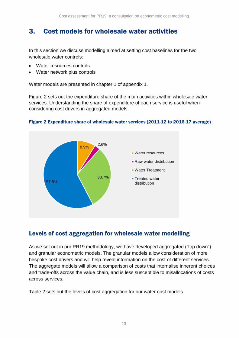
Figure 2 sets out the expenditure share of the main activities within wholesale water

services. Understanding the share of expenditure of each service is useful when

considering cost drivers in aggregated models.

Figure 2 Expenditure share of wholesale water services (2011-12 to 2016-17 average)

Levels of cost aggregation for wholesale water modelling

As we set out in our PR19 methodology, we have developed aggregated (“top down”)

and granular econometric models. The granular models allow consideration of more

bespoke cost drivers and will help reveal information on the cost of different services.

The aggregate models will allow a comparison of costs that internalise inherent choices

and trade-offs across the value chain, and is less susceptible to misallocations of costs

across services.

Table 2 sets out the levels of cost aggregation for our water cost models.

8.9%2.6%

30.7%57.8%

Water resources

Raw water distribution

Water Treatment

Treated waterdistribution


14

Table 2 Levels of aggregation for modelling in wholesale water

High level of aggregation Medium level of

aggregation

Low level of aggregation

Wholesale water Water resources plus

Water resources

Water network plus

Raw water transport

Water treatment

Treated water distribution

We think it is important to retain this range of options to estimate efficient costs for

different controls. For example, for water resources, we can use three types of models:

wholesale water models, water resources plus models and water resources models.

The middle level combines water resources, raw water transport and treatment. These

activities are closely linked as the water resources and treatment are often co-located on

the same operational site. This is often the case with borehole sites. The middle level

also avoids data allocation issues between the activities for costs such as power,

maintenance and land purchase.

The middle and high levels of aggregations will provide us with an estimate of efficient

costs at a more aggregated level than we need for our price controls. To use these

models to set efficient cost baselines for the PR19 controls, we will have to further split

the result. For example, using the wholesale water or wastewater models will require us

to split the results between the network plus and the water resources or bioresources

controls.

To do this split, we could use a company’s historical and forecast split between these

business units as a starting point. We welcome views on how this split can be done.

We are not presenting models for raw water transport. We have not obtained robust

enough models for this activity alone. At 2.6 percent of wholesale water costs, raw water

transport is the smallest ‘business unit’ in our accounting separation. Models based on

this data would be particularly susceptible to inconsistent allocation of costs by

companies.

Raw water transport data is included in models based on higher levels of aggregation,

such as water resources plus, network plus and wholesale water. If we use water

treatment and distribution models to set baselines for the water network plus controls, we

will consider an allowance for raw water transport separately, not on the basis of a

granular econometric model for this activity.


15

Figure 3 Breakdown of the 151 water models in this consultation

Costs excluded from our water models

The econometric models developed by Ofwat presented in this consultation cover base

costs7, which is operating costs plus capital maintenance costs. Our water models

exclude:

Abstraction charges/discharge consent

Business rates

Third party costs

Costs associated with the Traffic Management Act

Costs associated with statutory water softening

Enhancement capital expenditure (including infrastructure network reinforcement)

Pension deficit recovery payments

Atypical costs

We excluded costs associated with the Traffic Management Act, as these costs are

relevant only for a small number of companies. On this basis, we also excluded costs

associated with statutory water softening, as it affects only one company.

We excluded abstraction charges – charges levied by the Environment Agency for

abstraction licences from all levels of water models. While abstraction charges are linked

to the volume of water used by the company, we decided to exclude it from our models

for a number of reasons. Rebates made in 2014-15 and 2015-16 for the Environmental

Improvement Unit Charge (EIUC) and the fact that the EIUC is not under management

control and can vary drastically from company to company, mean that including

abstraction charges in the model can introduce a distortion. The rebates and the

7 Total base expenditure has become known as ‘botex’, analogous with totex, which stands for total expenditure.

144 7

40 382

108

8

8 12

16

10 1215

48 50

Waterresources

Watertreatment

WaterResources Plus

WaterDistribution

Network PlusWater

WholesaleWater



16

variation in EIUC are not necessarily related to underlying cost drivers for the company.

Further, a reform to abstraction charges due in the next period means that historical

levels of the charge may not be a good predictor of future levels.

Atypical costs can also present a distortion to modelling. These typically include

information on abstraction charge rebates and pension related items.

Our costs are gross of grants and contributions to have a better relationship between the

cost of the activity and the underlying drivers.

Cost drivers for wholesale water services

Table 3 sets out the main cost drivers that we considered at each part of the wholesale

water supply chain. We also discuss their expect effect on cost.

Table 3 Cost drivers of wholesale water services and expected effect on cost

Cost drivers Expected effect on cost

Water resources

All costs associated with the abstraction of raw water until it is delivered into the raw water distribution network.

Number of connected properties Measures of the scale of the business. Their correlation with cost is

strong and positive. When used as a primary scale variable in an econometric model the estimated coefficient would be positive. Volume of water abstracted

Average pumping head The larger the pumping head, the higher a cubic meter of water needs to be pumped and the higher the pumping costs. Average pumping head reflects topography and the volume of water pumped.

Number of sources This variable measures asset intensity. All else equal, a larger number of resources is expected to drive up water resources cost.

Proportion of water from boreholes

The source of water may affect pumping and maintenance costs. On average, we expect impounding reservoirs to have the lowest cost per unit of water. The other sources are more difficult to rank.

Proportion of water from rivers

Proportion of water from impounding reservoirs

Proportion of water from pumped storage reservoirs

Water treatment

All costs associated with the treatment of raw water at a water treatment works until it enters the treated water distribution network.

Number of connected properties Scale variables – see above

Volume of water treated


17

Distribution input

Proportion of water sourced from boreholes (including artificial recharge schemes and aquifer storage) The source of water affects the quality of raw water and the

complexity of treatment that has to be provided. On average boreholes can provide relatively high quality raw water which is cheapest to treat. River water is typically the most expensive to treat.

Proportion of water sourced from rivers

Proportion of water sourced from reservoirs (pumped storage and impounding)

Proportion of water treated at ‘complex’ water treatment works (eg at WTW types 3-6)

More complex water treatment works will typically have a higher cost of water treatment. The complexity reflects the quality of the water being received and/or the quality of the water requirements for the area supplied.

Average pumping head See above

Weighted average population density

A measure of population density at the company service area, constructed from ONS. The measures averages the density in each Lower Super Output Area (LSOA) and assigns higher weights to denser areas. For two companies of the same overall density (people/km2) this measure will tend to be larger for the company that has denser LSOAs.

For a water treatment business, the variable aims to capture the potential to use larger (and fewer) treatment works, with low unit treatment costs due to economies of scale.

Alongside a scale variable we expect a negative coefficient for this variable.

Treated water distribution

All costs associated with the distribution of treated water from the water treatment works to consumers.

Number of connected properties

Scale variables – see above Length of main

Distribution input

Average pumping head See above

Proportion of mains relined and renewed in the reporting year

A direct measure of activity, which will have a positive impact on maintenance costs.

Booster stations per km of mains

These variable are associated with network complexity. A more complex network will increase network costs.

Service reservoirs per km of mains

Water towers per km of mains

Proportion of new mains A measure of asset age. New assets are likely to require less maintenance. We expect a negative coefficient to this variable reflecting lower network costs.

Regional labour cost Regions with higher labour costs may incur higher costs to the extent that labour has to be sourced from, or operate in, the region.


18

4. Cost models for wholesale wastewater activities

In this section we present models aimed at setting cost baselines for wholesale

wastewater controls, which include

Bioresources controls

Wastewater network plus controls

Wastewater models are presented in chapter 2 of appendix 1.

Figure 4 sets out the expenditure share of the main activities within wholesale

wastewater services. Understanding the share of expenditure of each service is useful

when considering cost drivers in aggregated models.

Figure 4 Expenditure share of wholesale wastewater services (2011-12 to 2016-17

average)

Levels of cost aggregation for wholesale wastewater modelling

As we set out in our PR19 methodology, we have developed aggregated (“top down”)

and granular econometric models. Please refer to the discussion in the corresponding

section in chapter 3 for the rationale for this approach.

Table 4 sets out the levels of cost aggregation for our wastewater models.

35.2%

46.4%

18.3%

Sewage collection

Sewage treatment

Bioresources


19

Table 4 Levels of aggregation for modelling in wholesale wastewater

High level of aggregation Medium level of

aggregation

Low level of aggregation

Wholesale wastewater Wastewater network plus

Wastewater collection

Bioresources plus

Wastewater treatment

Bioresources

Figure 5 Breakdown of the 161 wastewater models in this consultation

Costs excluded from our wastewater models

The econometric models developed by Ofwat presented in this consultation cover base

costs, which is operating costs plus capital maintenance costs. Our wastewater models

exclude:

Business rates

Third party costs

Costs associated with the Traffic Management Act

Costs associated with the Industrial Emissions Directive

Enhancement capital expenditure (including infrastructure network reinforcement)

Pension deficit recovery payments

Atypical costs

We excluded costs associated with the Industrial Emissions Directive, as these were

incurred by a small number of companies, and historical levels of expenditure are

unlikely to be reflect the levels likely to be incurred in PR19.

34

7 7

3933

3

6

7

5

10

837

13

7

14

49

41

Bioresources SewageTreatment

BioresourcesPlus

SewageCollection

Network PlusWastewater

WholesaleWastewater



20

We discuss the reason for excluding these costs in the corresponding section in chapter

3.

Cost drivers for wholesale wastewater services

Table 5 sets out the main cost drivers that we considered at each part of the wholesale

wastewater supply chain. We also discuss their expect effect on cost.

Table 5 Cost drivers of wholesale wastewater services and expected effect on cost

Cost drivers Expected effect on cost

Sewage collection

All costs associated with collecting sewage from customers’ properties and transporting it to sewage treatment works.

Number of connected properties These are measures of the scale of the business. When used as a scale variable their correlation with cost is strong and positive.

We expect a positive sign to their coefficients.

Volume of wastewater

Sewer length

Number of connected properties per km of sewer

A measure of density. For equal sewer length, we expect this variable to be associated with higher costs, as there are more properties to collect sewage from.

Number of pumping stations per km of sewer

A measure of topography and asset intensity with an expected positive association with network costs.

Proportion of new sewers A measure of asset age. New assets are likely to require less maintenance.

We expect a negative coefficient to this variable reflecting lower network costs for higher proportions of new sewers.

Length of gravity sewer refurbished in the reporting year as a percentage of total sewer length

A direct measure of activity, which will increase maintenance costs if more sewers are refurbished.

Regional labour cost Regions with higher labour costs may incur higher costs to the extent that labour has to be sourced from, or operate in, the region. We note this may affect the cost of other services, not only distribution.

Sewage Treatment

All costs associated with operating and maintaining sewage treatment works to produce clean effluent for discharge to the environment and bioresources.

Load entering the sewage treatment works

A scale variable that accounts both for the volume and the strength of the sewage.

Volume of wastewater receiving treatment at sewage treatment works

An alternative scale variable that assumes that volume is a more significant driver of cost than sewage strength.

Number of connected properties A measure of scale expected to have a strong correlation with treatment costs.


21

Load treated in treatment works band sizes 1-3 as a percentage of total load

Larger treatment works typically have lower unit costs due to economies of scale. This variable captures sewage load treated in smaller works, which typically incur higher unit costs. We therefore expect a positive coefficient to this variable.

Load treated at sewage works with an ammonia consent equal to or below 1mg/l as a percentage of total load

Treatment costs will be affected by the effluent quality to which the wastewater needs to be treated. The tighter the consent the higher the cost of treatment.

We expect a positive sign to this coefficient.

Load from trade effluent customers as a percentage of total load

A proxy measure of treatment complexity. Trade effluent can have a higher COD/BOD ratio and be more difficult and, consequently, more expensive to treat compared to domestic sewage.

We expect a positive sign to this coefficient.

Bioresources

All costs associated with transporting sludge from sewage treatment works to the sludge treatment centre, its treatment, recycling and disposal.

Total sludge produced Measures of scale expected to have a strong, positive correlation with bioresources costs. Number of connected properties

Sludge disposed via farmland as a percentage of total sludge disposed

We expect that recycling treated sludge to farmland is cheaper than alternative methods of disposal.

We expect this variable to be negatively correlated with costs and therefore have a negative coefficient.

Total measure of intersiting work done (all forms of transportation)

A higher total intersiting work results from transporting sludge to a central treatment centre rather than treating sludge on the site where it was produced. All else being equal, we expect this variable to be positively correlated with costs.

Intersiting works done by road (trucks and tankers) as a percentage of total intersiting works

Road transport is expected to be more expensive than pipe transport of sludge from sewage treatment works to sludge treatment centres.


22

5. Cost models for residential retail activities

PR14 was the first time that we set a separate price control for retail activities. We used

an average costs to serve (ACTS) approach – we calculated the average retail cost per

customer in the sector, and used it as an upper-bound benchmark (ie companies were

allowed the lower of their forecast expenditure and the ACTS). This approach did not rely

on econometric modelling.

In our PR19 methodology we said that we intend to use an econometric modelling

approach to set efficient totex baselines for residential retail services.

Residential retail models are presented in chapter 3 of appendix 1.

Expenditure categories in residential retail

Residential retail represents around 9% of companies’ total expenditure. Figure 6 sets

out the relative share of the different types of costs in the residential retail business.

Figure 6 Expenditure share of residential retail services

Levels of cost aggregation for residential retail modelling

As outlined in our PR19 methodology we have developed three types of models in

residential retail.

Table 6 Levels of aggregation for residential retail modelling

Aggregated model Disaggregated models

Total retail costs (“RTC”) Bad debt plus debt management costs (“RDC”)

Other retail costs (“ROC”)

26%

9%

36%

5%

17%

7%

Customer services

Debt management

Doubtful Debts


23

Our choice of disaggregated models was motivated by considerations such as common

cost drivers, data quality (in particular cost allocation issues), and the level of interaction

between activities. We received overall support for this approach in our consultation on

the draft PR19 methodology.

We consider, for example, that bad debt and debt management costs are closely

interlinked. An increase in bad debt levels is likely to trigger an increase in debt

management costs, which in turn is likely to reduce bad debt level, and so on. Modelling

bad debt and debt management costs together would account for the inherent

operational choices and interactions between them. And keeping them separate from

other retail costs could allow us to better capture the specific relationship between debt

related costs and their unique drivers, such as bill size and deprivation.

Nonetheless, the disaggregated models that we selected are not immune to cost

allocation issues and to potential trade-offs between them. For this reason we have also

developed total retail costs models.

Figure 7 Breakdown of the 68 residential retail models in this consultation

Data for retail modelling

For the models presented in this consultation we used data from tables 2C and 2F of the

annual performance reports. The data covers the four-year period from 2013-14 to 2016-

17. The first three years include data on 18 companies, and the last year includes data

on 17 companies due to the merger of South West Water and Bournemouth Water, a

total of 71 observations.

For our bad debt models, we have used external data as a proxy for the probability that a

customer defaults on paying a water bill. We have tested deprivation measures such as

income, unemployment, job seekers allowance and the index of multiple deprivation

21

13

22

6

4

4

25

17

26

RDC ROC RTC



24

(IMD) sourced from official government statistics. We have also tested data from Equifax

on credit arrears risk provided to us by United Utilities. These variables have been

constructed from customer data to predict the likelihood that a customer will not pay their

bills.

Specification of the dependent variable in our retail models

We specified the dependent variable in all our retail models as retail cost per connected

household rather than as total costs. We considered that comparison of expenditure per

connected household was more intuitive given that retail costs are driven primarily by the

number of customers.

Specifying the dependent variable as cost per household does not, by itself, impose

restrictions on our models. In particular, it does not impose the restriction that costs vary

in the same proportion to the number of households (this is known as “constant returns

to scale”). To allow for economies of scale we have included a variable that relates to the

number of connected households as an explanatory variable in some of our models. This

would allow the model to identify a potential relationships between the number of

households served and the company’s average expenditure per household.

Cost drivers for retail activities

Table 7 sets out candidate drivers of bad debt and debt management costs.

Table 7 Cost drivers of retail activities and expected effect on cost

Main cost drivers Expected effect on retail cost

Bad debt costs including debt management costs

Provision for bad debt and all costs associated with managing bad debt and collecting outstanding customer revenues.

Total number of household customers

This is a primary cost driver of bad debt costs and retail costs can mostly be explained by customer numbers.

In our models, where the cost is specified as cost per household, this variable captures economies of scale. As such, we expect the coefficient to be zero or slightly negative, reflecting no or small economies of scale.

Average bill size Represents the amount of revenue that is at risk of not being paid should a default happens. We expect the average bill to have a strong correlation with bad debt per household.

Higher bills may also mean that the customer is more likely to default.

The propensity of default on payment

Bad debt and debt management costs will be higher for customers with a higher propensity to default.


25

We use proxies to control for the propensity to default in an area. These proxies are based on deprivation measures (eg income) and measures of arrears risk.

Changes in household occupancy (transience)

High transience rates can result in reduced ability to recover unpaid bills.

Other retail costs

All costs associated with meter reading, billing and payment handling, vulnerable customer schemes, customer enquiries and complaints handling, other operating costs, depreciation and amortisation.

Other operating costs include the provision of offices, insurance premiums, and local authority rates.

Total number of household customers

See above

Proportion of dual customers (household who receive both water and wastewater services from the same retailer)

A household customer who receives both water and waste water retail services may drive higher other retail costs compared to a customer who receives only a single service from the same retailer.

For example dual service households may generate more customer enquiries which may drive customer service costs.

We expect this measure to be positively correlated with other retail costs and the coefficient to have a small positive sign.

Proportion of metered household customers

A household customer who receives a metered service may drive higher retail costs through meter reading activity (although this is a relatively small proportion of other retail costs).

Also metered customers may generate more customer enquiries, for example they may be more likely to contact the retailer to query the meter readings that appear on their bills.

We expect this measure to be positively correlated with other retail costs and the coefficient to have a small positive sign.

Density / sparsity of metered properties

The distribution of customers may affect meter reading activity eg travel time to read meters in remote areas, traffic congestion in urban areas.

Our models do not include density or sparsity measures as these measures have not performed well. This may be because the costs associated with meter reading represent only a small proportion of other retail costs.

Quality of retail service A company may incur additional cost to provide better quality service. Likewise, a company may incur additional costs as a result of providing poor service. Evidence suggests that there is no clear relationship between cost and service quality. The relationship is not necessarily continuous or linear.

We have tested but not included a quality of service measure in our retail models. The estimated effect of such measure was not robust or consistent in our modelling. Moreover, our wider framework rewards outcomes associated with good customer service via the C-Mex mechanism.

Regional labour cost Regions with higher labour costs may incur higher costs to the extent that labour has to be sourced from, or operate in, the region. In our PR19 methodology we said that we do not intend to account for variation in regional labour costs in our benchmarking analysis for retail. We consider that the impact of regional labour costs can be substantially mitigated in most retail activities, as most retail activities are not bound by location.


26

6. Cost models for enhancement activities

Enhancement expenditure refers to expenditure for the purpose of enhancing the

capacity or quality of service beyond existing levels. This expenditure is generally not

routine, and is typically more difficult to compare across companies.

In our PR19 methodology we said that we would draw on a number of approaches to

assess different areas of enhancement. Some elements of enhancement expenditure

can be included with base costs in our econometric models. Other elements will be

assessed through a separate benchmarking analysis or through expert engineering

analysis.

In this consultation we present econometric models we have developed to date to

assess individual areas of enhancement expenditure for PR19.

Enhancement models are presented in chapter 4 of appendix 1.

Our work to develop cost assessment tools for enhancement expenditure is still in

progress. The models that we present in this consultation are those that we have

developed so far. We aim to explore further areas for modelling, in particular in light of

data that companies are due to submit in July 2018 and in their business plans.

One of the challenges in developing a statistical model for enhancement is data

availability. Our initial criteria for data availability were a sufficient number of

observations across company-years (we set 40 observations as a minimum threshold),

and a reasonable spread of expenditure across companies. We considered that no

company should account for more than 60% of the industry’s cumulative expenditure in

the 6-year period ending to 2016-17.

We smoothed the data for both the expenditure and cost drivers by applying a three-year

moving average. The smoothing mitigates the impact of the lumpy nature of capex

enhancement expenditure as well as reporting misalignments between the expenditure

and the driver of the expenditure.

Table identifies the enhancement activities that we modelled together and relevant cost

drivers.

Table 8 Enhancement expenditure models and cost drivers

Enhancement activities Relevant cost drivers

Meeting lead standards Scale: water delivered (potable); population served; zonal population receiving water treated with orthophosphate; number of lead communication pipes.


27

Activity/system characteristics: number of lead pipes replaced; % of lead pipes on total communication pipes; % of lead communication pipes replaced in total communication pipes.

Quality: mean zonal compliance; DWI lead test failures as a percentage of total tests.

New developments, including the new connections element (communication pipes, meters)

Scale/Activity: total number of household and non-household new connections; population served; water delivered (potable).

Other: time trend; density index.

First time sewerage Scale: number of properties connectable by S101A schemes.

Activity/system characteristics: number of S101A schemes; average number of connectable properties per S101A scheme; average resident population per S101A scheme.

New development and growth; growth at sewage treatment works; reduce sewer flooding risk for properties

Scale: resident population; volume of wastewater treated; number of household and non-household properties billed for sewerage.

Activity/system characteristics: total number of sewage treatment works; number of sewage treatment works in size band 5 and above; % of sewage treatment works in size band 5 and above; load per sewage treatment work; % of load treated in size bands 5 and above.

Ofwat (The Water Services Regulation Authority) is a non-ministerialgovernment department. We regulate the water sector in England andWales. Our vision is to be a trusted and respected regulator, working atthe leading edge, challenging ourselves and others to build trust andconfidence in water.

OfwatCentre City Tower7 Hill StreetBirmingham B5 4UA

Phone: 0121 644 7500Fax: 0121 644 7533Website: www.ofwat.gov.ukEmail: [email protected]

Printed on 75% minimum de-inked post-consumerwaste paper.March 2018

ISBN 978-1-911588-30-6

© Crown copyright 2018

This publication is licensed under the terms of theOpen Government Licence v3.0 except whereotherwise stated. To view this licence, visitnationalarchives.gov.uk/doc/open-government-licence/version/3 or write to the Information PolicyTeam, The National Archives, Kew, London TW9 4DU,or email [email protected].

Where we have identified any third party copyrightinformation, you will need to obtain permission fromthe copyright holders concerned.

This document is also available from our website atwww.ofwat.gov.uk.

Any enquiries regarding this publication should be sentto us at [email protected].

cost assessment for pr19: a consultation on … cost modelling trust in water. ... (pr19) for water...

Documents