cosmological physics - assetsassets.cambridge.org/0521422701/sample/0521422701ws.pdf · special...
TRANSCRIPT

COSMOLOGICAL PHYSICS
J. A . PEACOCK

pub l i s h ed by th e pr e s s s ynd i ca t e o f th e un i v e r s i t y o f cambr i dg eThe Pitt Building, Trumpington Street, Cambridge, United Kingdom
cambr i dg e un i v e r s i t y pr e s sThe Edinburgh Building, Cambridge CB2 2RU, UK40 West 20th Street, New York, NY 10011–4211, USA10 Stamford Road, Oakleigh, VIC 3166, AustraliaRuiz de Alarcon 13, 28014 Madrid, SpainDock House, The Waterfront, Cape Town 8001, South Africa
http://www.cambridge.org
c© Cambridge University Press 1999
This book is in copyright. Subject to statutory exceptionand to the provisions of relevant collective licensing agreements,no reproduction of any part may take place withoutthe written permission of Cambridge University Press.
First published 1999Reprinted 1999 (with corrections), 2000, 2001 (with corrections), 2002, 2003 (with corrections)
Printed in the United Kingdom at the University Press, Cambridge
Typeface Monotype Times 9 12/12pt System TEX [UPH]
A catalogue record for this book is available from the British Library
Library of Congress Cataloguing in Publication dataPeacock, John A.
Cosmological physics / J.A. Peacock.p. cm.
Includes bibliographical references and index.ISBN 0 521 41072 X (hardcover)1. Cosmology. 2. Astrophysics. I. Title.
QB981.P37 1999523.1–dc21 98-29460 CIP
ISBN 0 521 41072 X hardbackISBN 0 521 42270 1 paperback

Contents
Preface ix
Part 1: Gravitation and relativity
1 Essentials of general relativity 3
1.1 The concepts of general relativity 3
1.2 The equation of motion 9
1.3 Tensors and relativity 11
1.4 The energy–momentum tensor 17
1.5 The field equations 19
1.6 Alternative theories of gravity 26
1.7 Relativity and differential geometry 28
2 Astrophysical relativity 35
2.1 Relativistic fluid mechanics 35
2.2 Weak fields 38
2.3 Gravitational radiation 42
2.4 The binary pulsar 49
2.5 Black holes 51
2.6 Accretion onto black holes 60
Part 2: Classical cosmology
3 The isotropic universe 65
3.1 The Robertson–Walker metric 65
3.2 Dynamics of the expansion 72
3.3 Common big bang misconceptions 86
3.4 Observations in cosmology 89
3.5 The anthropic principle 94
4 Gravitational lensing 101
4.1 Basics of light deflection 101
4.2 Simple lens models 105
4.3 General properties of thin lenses 109

vi Contents
4.4 Observations of gravitational lensing 113
4.5 Microlensing 116
4.6 Dark-matter mapping 121
5 The age and distance scales 127
5.1 The distance scale and the age of the universe 127
5.2 Methods for age determination 128
5.3 Large-scale distance measurements 134
5.4 The local distance scale 138
5.5 Direct distance determinations 141
5.6 Summary 145
Part 3: Basics of quantum fields
6 Quantum mechanics and relativity 151
6.1 Principles of quantum theory 151
6.2 The Dirac equation 158
6.3 Symmetries 164
6.4 Spinors and complex numbers 167
7 Quantum field theory 177
7.1 Quantum mechanics of light 177
7.2 Simple quantum electrodynamics 181
7.3 Lagrangians and fields 184
7.4 Interacting fields 189
7.5 Feynman diagrams 197
7.6 Renormalization 205
7.7 Path integrals 210
8 The standard model and beyond 215
8.1 Elementary particles and fields 215
8.2 Gauge symmetries and conservation laws 216
8.3 The weak interaction 220
8.4 Non-Abelian gauge symmetries 223
8.5 Spontaneous symmetry breaking 228
8.6 The electroweak model 232
8.7 Quantum chromodynamics 236
8.8 Beyond the standard model 245
8.9 Neutrino masses and mixing 251
8.10 Quantum gravity 256
8.11 Kaluza–Klein models 265
8.12 Supersymmetry and beyond 267
Contents vii
Part 4: The early universe
9 The hot big bang 273
9.1 Thermodynamics in the big bang 273
9.2 Relics of the big bang 282
9.3 The physics of recombination 284
9.4 The microwave background 288
9.5 Primordial nucleosynthesis 292
9.6 Baryogenesis 300
10 Topological defects 305
10.1 Phase transitions in cosmology 305
10.2 Classes of topological defect 306
10.3 Magnetic monopoles 310
10.4 Cosmic strings and structure formation 313
11 Inflationary cosmology 323
11.1 General arguments for inflation 323
11.2 An overview of inflation 325
11.3 Inflation field dynamics 328
11.4 Inflation models 335
11.5 Relic fluctuations from inflation 338
11.6 Conclusions 347
Part 5: Observational cosmology
12 Matter in the universe 353
12.1 Background radiation 353
12.2 Intervening absorbers 360
12.3 Evidence for dark matter 367
12.4 Baryonic dark matter 378
12.5 Nonbaryonic dark matter 381
13 Galaxies and their evolution 387
13.1 The galaxy population 387
13.2 Optical and infrared observations 394
13.3 Luminosity functions 399
13.4 Evolution of galaxy stellar populations 404
13.5 Galaxy counts and evolution 406
13.6 Galaxies at high redshift 412
14 Active galaxies 419
14.1 The population of active galaxies 419
14.2 Emission mechanisms 423
14.3 Extended radio sources 431
14.4 Beaming and unified schemes 437
14.5 Evolution of active galaxies 441

viii Contents
14.6 Black holes as central engines 447
14.7 Black hole masses and demographics 451
Part 6: Galaxy formation and clustering
15 Dynamics of structure formation 457
15.1 Overview 458
15.2 Dynamics of linear perturbations 460
15.3 The peculiar velocity field 469
15.4 Coupled perturbations 471
15.5 The full treatment 474
15.6 Transfer functions 477
15.7 N-body models 482
15.8 Nonlinear models 485
16 Cosmological density fields 495
16.1 Preamble 495
16.2 Fourier analysis of density fluctuations 496
16.3 Gaussian density fields 503
16.4 Nonlinear clustering evolution 509
16.5 Redshift-space effects 514
16.6 Low-dimensional density fields 517
16.7 Measuring the clustering spectrum 521
16.8 The observed clustering spectrum 526
16.9 Non-Gaussian density fields 536
16.10 Peculiar velocity fields 543
17 Galaxy formation 553
17.1 The sequence of galaxy formation 553
17.2 Hierarchies and the Press–Schechter approach 556
17.3 Cooling and the intergalactic medium 569
17.4 Chemical evolution of galaxies 575
17.5 Biased galaxy formation 578
18 Cosmic background fluctuations 587
18.1 Mechanisms for primary fluctuations 587
18.2 Characteristics of CMB anisotropies 597
18.3 Observations of CMB anisotropies 601
18.4 Conclusions and outlook 603
H ints for solution of the problems 613
Bibliography and references 647
Useful numbers and formulae 663
Index 671

1 Essentials of general relativity
1.1 The concepts of general relativity
special relativity To understand the issues involved in general relativity, it is
helpful to begin with a brief summary of the way space and time are treated in special
relativity. The latter theory is an elaboration of the intuitive point of view that the
properties of empty space should be the same throughout the universe. This is just a
generalization of everyday experience: the world in our vicinity looks much the same
whether we are stationary or in motion (leaving aside the inertial forces experienced by
accelerated observers, to which we will return shortly).
The immediate consequence of this assumption is that any process that depends
only on the properties of empty space must appear the same to all observers: the velocity
of light or gravitational radiation should be a constant. The development of special
relativity can of course proceed from the experimental constancy of c, as revealed by
the Michelson-Morley experiment, but it is worth noting that Einstein considered the
result of this experiment to be inevitable on intuitive grounds (see Pais 1982 for a
detailed account of the conceptual development of relativity). Despite the mathematical
complexity that can result, general relativity is at heart a highly intuitive theory; the way
in which our everyday experience can be generalized to deduce the large-scale structure
of the universe is one of the most magical parts of physics. The most important concepts
of the theory can be dealt with without requiring much mathematical sophistication, and
we begin with these physical fundamentals.
4-vectors From the constancy of c, it is simple to show that the only possible linear
transformation relating the coordinates measured by different observers is the Lorentz
transformation:
dx′ = γ(dx − v
cc dt)
c dt′ = γ(c dt − v
cdx).
(1.1)
Note that this is written in a form that makes it explicit that x and ct are treated in the
same way. To reflect this interchangeability of space and time, and the absence of any
preferred frame, we say that special relativity requires all true physical relations to be
written in terms of 4-vectors. An equation valid for one observer will then apply to all

4 1 Essentials of general relativity
others because the quantities on either side of the equation will transform in the same
way. We ensure that this is so by constructing physical 4-vectors out of the fundamental
interval
dxµ = (c dt, dx, dy, dz) µ = 0, 1, 2, 3, (1.2)
by manipulations with relativistic invariants such as rest mass m and proper time dτ,
where
(c dτ)2 = (c dt)2 − (dx2 + dy2 + dz2). (1.3)
Thus, defining the 4-momentum Pµ = mdxµ/dτ allows an immediate relativistic
generalization of conservation of mass and momentum, since the equation ∆Pµ = 0
reduces to these laws for an observer who sees a set of slowly moving particles. This
is a very powerful principle, as it allows us to reject ‘obviously wrong’ physical laws
at sight. For example, Newton’s second law F = mdu/dt is not a relation between the
spatial components of two 4-vectors. The obvious way to define 4-force is Fµ = dPµ/dτ,
but where does the 3-force F sit in Fµ? Force will still be defined as rate of change
of momentum, F = dP/dt; the required components of Fµ are γ(E,F), and the correct
relativistic force–acceleration relation is
F = md
dt(γu). (1.4)
Note again that the symbol m denotes the rest mass of the particle, which is one of
the invariant scalar quantities of special relativity. The whole ethos of special relativity
is that, in the frame in which a particle is at rest, its intrinsic properties such as mass
are always the same, independently of how fast it is moving. The general way in which
quantities are calculated in relativity is to evaluate them in the rest frame where things
are simple, and then to transform out into the lab frame.
general relativity Nothing that has been said so far seems to depend on whether
or not observers move at constant velocity. We have in fact already dealt with the main
principle of general relativity, which states that the only valid physical laws are those
that equate two quantities that transform in the same way under any arbitrary change
of coordinates.
Before getting too pleased with ourselves, we should ask how we are going to
construct general analogues of 4-vectors. Consider how the components of dxµ transform
under the adoption of a new set of coordinates x′µ, which are functions of xν:
dx′µ =∂x′µ∂xν
dxν . (1.5)
This apparently trivial equation (which assumes, as usual, the summation convention on
repeated indices) may be divided by dτ on either side to obtain a similar transformation
law for 4-velocity, Uµ; so Uµ is a general 4-vector. Things unfortunately go wrong at
the next level, when we try to differentiate this new equation to form the 4-acceleration
Aµ = dUµ/dτ:
A′µ =∂x′µ∂xν
Aν +∂2x′µ∂τ ∂xν
Uν. (1.6)

1.1 The concepts of general relativity 5
The second term on the right-hand side (rhs) is zero only when the transformation
coefficients are constants. This is so for the Lorentz transformation, but not in general.
The conclusion is therefore that Fµ = dPµ/dτ cannot be a general law of physics, since
dPµ/dτ is not a general 4-vector.
inertial frames and mach’s principle We have just deduced in a rather
cumbersome fashion the familiar fact that F = ma only applies in inertial frames
of reference. What exactly are these? There is a well-known circularity in Newtonian
mechanics, in that inertial frames are effectively defined as being those sets of observers
for whom F = ma applies. The circularity is only broken by supplying some independent
information about F – for example, the Lorentz force F = e(E + v∧B) in the case of a
charged particle. This leaves us in a rather unsatisfactory situation: F = ma is really only
a statement about cause and effect, so the existence of non-inertial frames comes down
to saying that there can be a motion with no apparent cause. Now, it is well known that
F = ma can be made to apply in all frames if certain ‘fictitious’ forces are allowed to
operate. In respectively uniformly accelerating and rotating frames, we would write
F = ma + mg
F = ma + mΩ∧(Ω∧r) − 2m(v∧Ω) + mΩ∧r.(1.7)
The fact that these ‘forces’ have simple expressions is tantalizing: it suggests that they
should have a direct explanation, rather than taking the Newtonian view that they arise
from an incorrect choice of reference frame. The relativist’s attitude will be that if our
physical laws are correct, they should account for what observers see from any arbitrary
point of view – however perverse.
The mystery of inertial frames is deepened by a fact of which Newton was well
aware, but did not explain: an inertial frame is one in which the bulk of matter in the
universe is at rest. This observation was taken up in 1872 by Ernst Mach. He argued
that since the acceleration of particles can only be measured relative to other matter in
the universe, the existence of inertia for a particle must depend on the existence of other
matter. This idea has become known as Mach’s principle, and was a strong influence on
Einstein in formulating general relativity. In fact, Mach’s ideas ended up very much in
conflict with Einstein’s eventual theory – most crucially, the rest mass of a particle is a
relativistic invariant, independent of the gravitational environment in which a particle
finds itself. However, controversy still arises in debating whether general relativity is
truly a ‘Machian’ theory – i.e. one in which the rest frame of the large-scale matter
distribution is inevitably an inertial frame (e.g. Raine & Heller 1981).
A hint at the answer to this question comes by returning to the expressions for
the inertial forces. The most satisfactory outcome would be to dispose of the notion
of inertial frames altogether, and to find a direct physical mechanism for generating
‘fictitious’ forces. Following this route in fact leads us to conclude that Newtonian
gravitation cannot be correct, and that the inertial forces can be effectively attributed to
gravitational radiation. Since we cannot at this stage give a correct relativistic argument,
consider the analogy with electromagnetism. At large distances, an accelerating charge
produces an electric field given by
E =e
4πε0rc2(r∧[a])∧ r, (1.8)
i.e. with components parallel to the retarded acceleration [a] and perpendicular to the
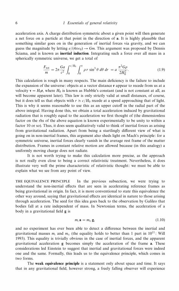
6 1 Essentials of general relativity
acceleration axis. A charge distribution symmetric about a given point will then generate
a net force on a particle at that point in the direction of a. It is highly plausible that
something similar goes on in the generation of inertial forces via gravity, and we can
guess the magnitude by letting e/(4πε0) → Gm. This argument was proposed by Dennis
Sciama, and is known as inertial induction. Integrating such a force over all mass in a
spherically symmetric universe, we get a total of
Ftot
m= 2π
Ga
c2
∫ c/H0
0
∫ π
0
ρ r sin3 θ dθ dr = aπ2Gρ
2H20
. (1.9)
This calculation is rough in many respects. The main deficiency is the failure to include
the expansion of the universe: objects at a vector distance r appear to recede from us at a
velocity v = H0r, where H0 is known as Hubble’s constant (and is not constant at all, as
will become apparent later). This law is only strictly valid at small distances, of course,
but it does tell us that objects with r c/H0 recede at a speed approaching that of light.
This is why it seems reasonable to use this as an upper cutoff in the radial part of the
above integral. Having done this, we obtain a total acceleration induced by gravitational
radiation that is roughly equal to the acceleration we first thought of (the dimensionless
factor on the rhs of the above equation is known experimentally to be unity to within a
factor 10 or so). Thus, it does seem qualitatively valid to think of inertial forces as arising
from gravitational radiation. Apart from being a startlingly different view of what is
going on in non-inertial frames, this argument also sheds light on Mach’s principle: for a
symmetric universe, inertial forces clearly vanish in the average rest frame of the matter
distribution. Frames in constant relative motion are allowed because (in this analogy) a
uniformly moving charge does not radiate.
It is not worth trying to make this calculation more precise, as the approach
is not really even close to being a correct relativistic treatment. Nevertheless, it does
illustrate very well the prime characteristic of relativistic thought: we must be able to
explain what we see from any point of view.
the equivalence principle In the previous subsection, we were trying to
understand the non-inertial effects that are seen in accelerating reference frames as
being gravitational in origin. In fact, it is more conventional to state this equivalence the
other way around, saying that gravitational effects are identical in nature to those arising
through acceleration. The seed for this idea goes back to the observation by Galileo that
bodies fall at a rate independent of mass. In Newtonian terms, the acceleration of a
body in a gravitational field g is
mI a = mG g, (1.10)
and no experiment has ever been able to detect a difference between the inertial and
gravitational masses mI and mG (the equality holds to better than 1 part in 1011: Will
1993). This equality is trivially obvious in the case of inertial forces, and the apparent
gravitational acceleration g becomes simply the acceleration of the frame a. These
considerations led Einstein to suggest that inertial and gravitational forces were indeed
one and the same. Formally, this leads us to the equivalence principle, which comes in
two forms.
The weak equivalence principle is a statement only about space and time. It says
that in any gravitational field, however strong, a freely falling observer will experience

1.1 The concepts of general relativity 7
no gravitational effects – with the important exception of tidal forces in non-uniform
fields. The spacetime will be that of special relativity (known as Minkowski spacetime).
The strong equivalence principle takes this a stage further and asserts that not
only is the spacetime as in special relativity, but all the laws of physics take the same
form in the freely falling frame as they would in the absence of gravity. This form of
the equivalence principle is crucial in that it will allow us to deduce the generally valid
laws governing physics once the special-relativistic forms are known. Note however that
it is less easy to design experiments that can test the strong equivalence principle (see
chapter 8 of Will 1993).
It may seem that we have actually returned to something like the Newtonian
viewpoint: gravitation is merely an artifact of looking at things from the ‘wrong’ point
of view. This is not really so; rather, the important aspects of gravitation are not so much
to do with first-order effects as second-order tidal forces: these cannot be transformed
away and are the true signature of gravitating mass. However, it is certainly true in one
sense to say that gravity is not a real force: the gravitational acceleration is not derived
from a 4-force Fµ and transforms differently.
gravitational time dilation Many of the important features of general relativity
can be obtained via rather simple arguments that use the equivalence principle. The
most famous of these is the thought experiment that leads to gravitational time dilation,
illustrated in figure 1.1. Consider an accelerating frame, which is conventionally a rocket
of height h, with a clock mounted on the roof that regularly disgorges photons towards
the floor. If the rocket accelerates upwards at g, the floor acquires a speed v = gh/c in
the time taken for a photon to travel from roof to floor. There will thus be a blueshift
in the frequency of received photons, given by ∆ν/ν = gh/c2, and it is easy to see that
the rate of reception of photons will increase by the same factor.
Now, since the rocket can be kept accelerating for as long as we like, and since
photons cannot be stockpiled anywhere, the conclusion of an observer on the floor of the
rocket is that in a real sense the clock on the roof is running fast. When the rocket stops
accelerating, the clock on the roof will have gained a time ∆t by comparison with an
identical clock kept on the floor. Finally, the equivalence principle can be brought in to
conclude that gravity must cause the same effect. Noting that ∆φ = gh is the difference
in potential between roof and floor, it is simple to generalize this to
∆t
t=
∆φ
c2. (1.11)
The same thought experiment can also be used to show that light must be deflected
in a gravitational field: consider a ray that crosses the rocket cabin horizontally when
stationary. This track will appear curved when the rocket accelerates.
The experimental demonstration of the gravitational redshift by Pound & Rebka
(1960) was one of the main pieces of evidence for the essential correctness of the above
reasoning, and provides a test (although not the most powerful one) of the equivalence
principle.
the twin paradox One of the neatest illustrations of gravitational time dilation is
in resolving the twin paradox. This involves twins A and B, each equipped with a clock.

8 1 Essentials of general relativity
cg
cg
Figure 1.1. Imagine you are in a box in free space far from any sourceof gravitation. If the box is made to accelerate ‘upwards’ and has a clockthat emits a photon every second mounted on its roof, it is easy to see thatyou will receive photons more rapidly once the box accelerates (imagineyourself running into the line of oncoming photons). Now, according tothe equivalence principle, the situation is exactly equivalent to the secondpicture in which the box sits at rest on the surface of the Earth. Since thereis nowhere for the excess photons to accumulate, the conclusion has to bethat clocks above us in a gravitational field run fast.
A remains on Earth, while B travels a distance d on a rocket at velocity v, fires the
engines briefly to reverse the rocket’s velocity, and returns. The standard analysis of this
situation in special relativity concludes, correctly, that A’s clock will indicate a longer
time for the journey than B’s:
tA = γ tB. (1.12)
The so-called paradox lies in the broken symmetry between the twins. There are various
resolutions of this puzzle, but these generally refuse to meet the problem head-on by
analysing things from B’s point of view. However, at least for small v, it is easy to do
this using the equivalence principle. There are three stages to consider:
(1) Outward trip. According to B, in special relativity A’s clock runs slow:
tA = γ−1tB [1 − v2/(2c2)](d/v).
(2) Return trip. Similarly, A’s clock runs slow, resulting in a total lag with respect to
B’s of (v2/c2)(d/v) = vd/c2.
1.2 The equation of motion 9
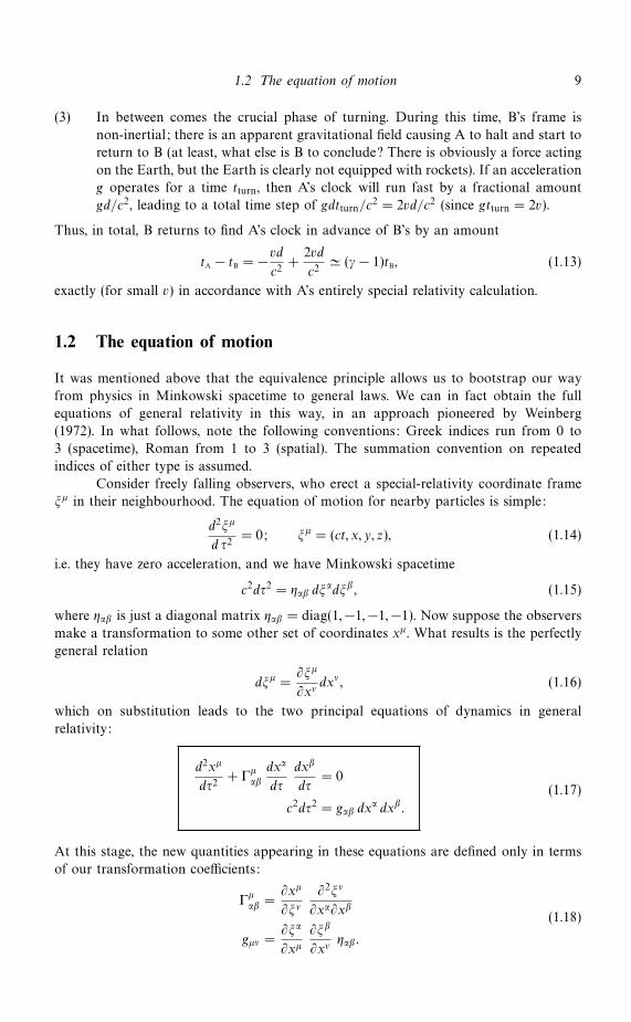
(3) In between comes the crucial phase of turning. During this time, B’s frame is
non-inertial; there is an apparent gravitational field causing A to halt and start to
return to B (at least, what else is B to conclude? There is obviously a force acting
on the Earth, but the Earth is clearly not equipped with rockets). If an acceleration
g operates for a time tturn, then A’s clock will run fast by a fractional amount
gd/c2, leading to a total time step of gdtturn/c2 = 2vd/c2 (since gtturn = 2v).
Thus, in total, B returns to find A’s clock in advance of B’s by an amount
tA − tB = − vd
c2+
2vd
c2 (γ − 1)tB, (1.13)
exactly (for small v) in accordance with A’s entirely special relativity calculation.
1.2 The equation of motion
It was mentioned above that the equivalence principle allows us to bootstrap our way
from physics in Minkowski spacetime to general laws. We can in fact obtain the full
equations of general relativity in this way, in an approach pioneered by Weinberg
(1972). In what follows, note the following conventions: Greek indices run from 0 to
3 (spacetime), Roman from 1 to 3 (spatial). The summation convention on repeated
indices of either type is assumed.
Consider freely falling observers, who erect a special-relativity coordinate frame
ξµ in their neighbourhood. The equation of motion for nearby particles is simple:
d2ξµ
d τ2= 0; ξµ = (ct, x, y, z), (1.14)
i.e. they have zero acceleration, and we have Minkowski spacetime
c2dτ2 = ηαβ dξαdξβ, (1.15)
where ηαβ is just a diagonal matrix ηαβ = diag(1,−1,−1,−1). Now suppose the observers
make a transformation to some other set of coordinates xµ. What results is the perfectly
general relation
dξµ =∂ξµ
∂xνdxν , (1.16)
which on substitution leads to the two principal equations of dynamics in general
relativity:
d2xµ
dτ2+ Γ
µαβ
dxα
dτ
dxβ
dτ= 0
c2dτ2 = gαβ dxα dxβ.
(1.17)
At this stage, the new quantities appearing in these equations are defined only in terms
of our transformation coefficients:
Γµαβ =
∂xµ
∂ξν∂2ξν
∂xα∂xβ
gµν =∂ξα
∂xµ∂ξβ
∂xνηαβ.
(1.18)

10 1 Essentials of general relativity
coordinate transformations What is the physical meaning of this analysis? We
have taken the special relativity equations for motion and the structure of spacetime
and looked at the effects of a general coordinate transformation. One example of such
a transformation is a Lorentz boost to some other inertial frame. However, this is not
very interesting since we know in advance that the equations retain their form in this
case (it is easy to show that Γµαβ = 0 and gµν = ηµν). A more general transformation
could be one to the frame of an accelerating observer, but the transformation might have
no direct physical interpretation at all. It is important to realize that general relativity
makes no distinction between coordinate transformations associated with motion of the
observer and a simple change of variable. For example, we might decide that henceforth
we will write down coordinates in the order (x, y, z, ct) rather than (ct, x, y, z) (as is
indeed the case in some formalisms). General relativity can cope with these changes
automatically. Indeed, this flexibility of the theory is something of a problem: it can
sometimes be hard to see when some feature of a problem is ‘real’, or just an artifact
of the coordinates adopted. People attempt to distinguish this second type of coordinate
change by distinguishing between ‘active’ and ‘passive’ Lorentz transformations; a more
common term for the latter class is gauge transformation. The term gauge will occur
often throughout this book: it always refers to some freedom within a theory that has no
observable consequence (e.g. the arbitrary value of ∇∇∇∇∇∇∇∇∇∇∇∇∇ · A, where A is the vector potential
in electrodynamics).
metric and connection The matrix gµν is known as the metric tensor. It expresses
(in the sense of special relativity) a notion of distance between spacetime points. Although
this is a feature of many spaces commonly used in physics, it is easy to think of cases
where such a measure does not exist (for example, in a plot of particle masses against
charges, there is no physical meaning to the distance between points). The fact that
spacetime is endowed with a metric is in fact something that has been deduced , as a
consequence of special relativity and the equivalence principle. Given a metric, Minkowski
spacetime appears as an inevitable special case: if the matrix gµν is symmetric, we know
that there must exist a coordinate transformation that makes the matrix diagonal:
ΛgΛ = diag(λ0, . . . , λ3), (1.19)
where Λ is the matrix of transformation coefficients, and λi are the eigenvalues of this
matrix.
The object gµν is called a tensor, since it occurs in an equation c2dτ2 = gµνdxµdxν
that must be valid in all frames. In order for this to be so, the components of the matrix
g must obey certain transformation relations under a change of coordinates. This is one
way of defining a tensor, an issue that is discussed in detail below.
So much for the metric tensor, what is the meaning of the coefficients Γµαβ?
These are known as components of the affine connection or as Christoffel symbols (and
are sometimes written in the alternative notation µαβ ). These quantities obviously
correspond roughly to the gravitational force – but what determines whether such a
force exists? The answer is that gravitational acceleration depends on spatial change in
the metric. For a simple example, consider gravitational time dilation in a weak field:
for events at the same spatial position, there must be a separation in proper time of
dτ dt
(1 +
∆φ
c2
). (1.20)

1.3 Tensors and relativity 11
This suggests that the gravitational acceleration should be obtained via
a = −c2
2∇∇∇∇∇∇∇∇∇∇∇∇∇g00. (1.21)
More generally, we can differentiate the equation for gµν to get
∂gµν
∂xλ= Γα
λµgαν + Γβλνgβµ. (1.22)
Using the symmetry of the Γ’s in their lower indices, and defining gµν to be the matrix
inverse to gµν , we can find an equation for the Γ’s directly in terms of the metric tensor:
Γαλµ = 1
2gαν
(∂gµν
∂xλ+
∂gλν
∂xµ− ∂gµλ
∂xν
). (1.23)
Thus, the metric tensor is the crucial object in general relativity: given it, we know both
the structure of spacetime and how particles will move.
1.3 Tensors and relativity
Before proceeding further, the above rather intuitive treatment should be set on a slightly
firmer mathematical foundation. There are a variety of possible approaches one can take,
which differ sufficiently that general relativity texts for physicists and mathematicians
sometimes scarcely seem to refer to the same subject. For now, we stick with a rather
old-fashioned approach, which has the virtue that it is likely to be familiar. Amends will
be made later.
covariant and contravariant components So far, tensors have been met in
their role as quantities that provide generally valid relations between different 4-vectors. If
such relations are to be physically useful, they must apply in different frames of reference,
and so the components of tensors have to change to compensate for the fact that the
components of 4-vectors alter under a coordinate transformation. The transformation law
for tensors is obtained from that for 4-vectors. For example, consider c2dτ2 = gαβdxαdxβ:
substitute for dxµ in terms of dx′α and require that the resulting equation must have the
form c2dτ2 = g′αβdx
′αdx′β . We then deduce the tensor transformation law
g′αβ =
∂xµ
∂x′α∂xν
∂x′β gµν , (1.24)
of which law our above definition of gµν in terms of ηαβ is an example.
Note that this transformation law looks rather like a generalization of that for a
single 4-vector (with one transformation coefficient per index), but with the important
difference that the coefficients are upside down in the tensor relation. For Cartesian
coordinates, this would make no difference:
∂xµ
∂x′α =∂x′α∂xµ
= cos θ, (1.25)
where θ is the angle of rotation between the two coordinate axes. In general, though,

12 1 Essentials of general relativity
the transformations are not the same. To illustrate this, consider a set of non-orthogonal
basis vectors ei: there are two ways to define the components of a vector a:
(1) a =∑
aiei
(2) ai = a · ei.(1.26)
These clearly differ in general if ei · ej = 0, and they are distinguished by writing an
index ‘upstairs’ on one and ‘downstairs’ on the other.
Something very similar goes on in general relativity. If we define a new vector
dxν ≡ gανdxα, (1.27)
then our metric is given by
c2dτ2 = dxνdxν . (1.28)
In special relativity, this would yield just xµ = (ct,−x,−y,−z). In general relativity, it
defines the relations between the contravariant components of a 4-vector Aµ and the
covariant components Aµ. These names reflect that the components transform either in
the same way as basis vectors (covariant) or oppositely (contravariant). The relevant
transformation laws are
A′µ =∂x′µ∂xν
Aν
A′µ =
∂xν
∂x′µ Aν .
(1.29)
This generalizes to any tensor, by multiplying by the appropriate factor for each index.
invariants To summarize the above arguments, one can only construct an invariant
quantity in general relativity (i.e. one that is the same for all observers) by contracting
vector or tensor indices in pairs: AµAµ is the invariant ‘size’ or norm of the vector Aµ.
However, AµAµ would not be a constant, since the effects of arbitrary coordinate changes
do not cancel out unless upstairs and downstairs indices contract with each other.
This sounds like a tedious complication, but it can be turned to advantage.
Suppose we are given an equation such as AµBµ = 1, and that Aµ is known to be a
4-vector. Clearly, the right-hand side of the equation is invariant, and so the only way
in which this can happen in general is if Bµ is also a 4-vector. This trick of deducing the
nature of quantities in a relativistic equation is called the principle of manifest covariance.
As an example, consider the coordinate derivative, for which there exists the common
shorthand
∂µ ≡ ∂
∂xµ. (1.30)
The index must be ‘downstairs’ since the derivative operates only on one coordinate:
∂µxν = δνµ = diag(1, 1, 1, 1). (1.31)
Thus, ∂µxµ = 4 is an invariant, justifying the use of a downstairs index for ∂µ. More
generally, the tensor δνµ must be an isotropic tensor (meaning one whose components are
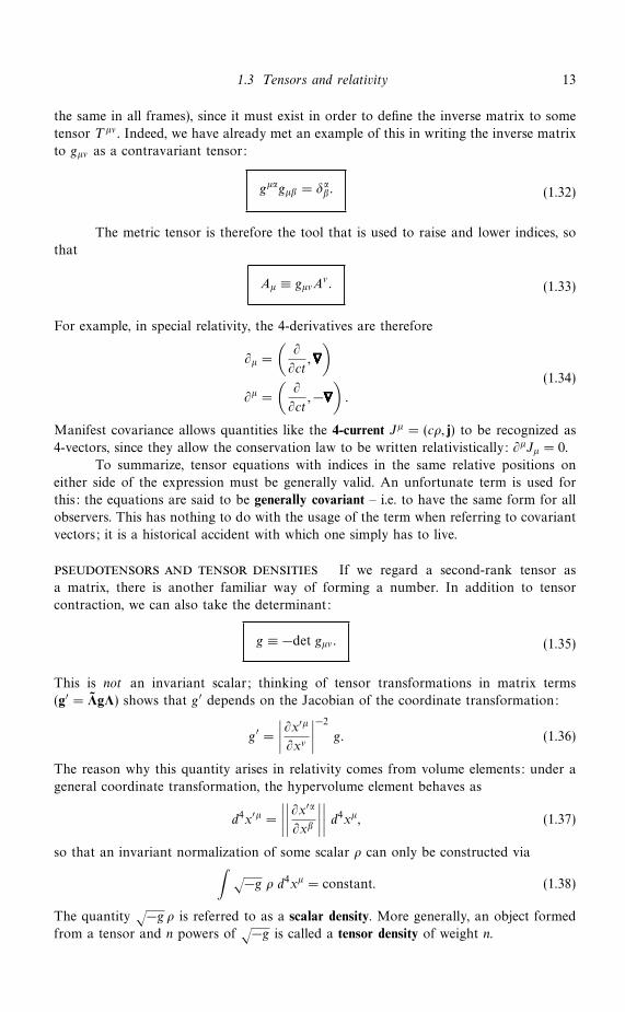
1.3 Tensors and relativity 13
the same in all frames), since it must exist in order to define the inverse matrix to some
tensor Tµν . Indeed, we have already met an example of this in writing the inverse matrix
to gµν as a contravariant tensor:
gµαgµβ = δαβ. (1.32)
The metric tensor is therefore the tool that is used to raise and lower indices, so
that
Aµ ≡ gµνAν . (1.33)
For example, in special relativity, the 4-derivatives are therefore
∂µ =
(∂
∂ct,∇∇∇∇∇∇∇∇∇∇∇∇∇)
∂µ =
(∂
∂ct,−∇∇∇∇∇∇∇∇∇∇∇∇∇
).
(1.34)
Manifest covariance allows quantities like the 4-current Jµ = (cρ, j) to be recognized as
4-vectors, since they allow the conservation law to be written relativistically: ∂µJµ = 0.
To summarize, tensor equations with indices in the same relative positions on
either side of the expression must be generally valid. An unfortunate term is used for
this: the equations are said to be generally covariant – i.e. to have the same form for all
observers. This has nothing to do with the usage of the term when referring to covariant
vectors; it is a historical accident with which one simply has to live.
pseudotensors and tensor densities If we regard a second-rank tensor as
a matrix, there is another familiar way of forming a number. In addition to tensor
contraction, we can also take the determinant:
g ≡ −det gµν . (1.35)
This is not an invariant scalar; thinking of tensor transformations in matrix terms
(g′ = ΛgΛ) shows that g′ depends on the Jacobian of the coordinate transformation:
g′ =
∣∣∣∣∂x′µ∂xν
∣∣∣∣−2
g. (1.36)
The reason why this quantity arises in relativity comes from volume elements: under a
general coordinate transformation, the hypervolume element behaves as
d4x′µ =
∣∣∣∣∣∣∣∣∂x′α∂xβ
∣∣∣∣∣∣∣∣ d4xµ, (1.37)
so that an invariant normalization of some scalar ρ can only be constructed via∫ √−g ρ d4xµ = constant. (1.38)
The quantity√−g ρ is referred to as a scalar density. More generally, an object formed
from a tensor and n powers of√−g is called a tensor density of weight n.

14 1 Essentials of general relativity
proper and improper transformations One important consequence of the
existence of tensor densities arises when considering coordinate transformations that
involve a spatial reflection. It is usual to distinguish between different classes of Lorentz
transformations according to the sign of their corresponding Jacobians: proper Lorentz
transformations have J > 0, whereas those with negative Jacobians are termed improper.
In special relativity, where g = −1 always, there are two possibilities: J = ±1. Thus, a
tensor density will in special relativity transform like a tensor if we restrict ourselves to
proper transformations. However, on spatial inversion, densities of odd weight will change
sign. Such quantities are referred to as pseudotensors (or, in special cases pseudovectors
or pseudoscalars). The most famous example of this is the totally antisymmetric Levi–
Civita pseudotensor εαβγδ , which has components +1 when αβγδ is an even permutation
of 0123, −1 for odd permutations and zero otherwise. One can show explicitly that
this frame-independent component definition produces a tensor density of weight −1
by applying the transformation law for such a quantity and verifying the invariance
of the components (not too hard since ε enters into the definition of the determinant).
Lowering indices with the metric tensor produces a covariant density of weight −1:
εαβγδ = gεαβγδ . (1.39)
In special relativity, εαβγδ is therefore of opposite sign to εαβγδ .
physics in general relativity So far, we have dealt with how to generalize
gravitational dynamics, but how are other parts of physics incorporated into general
relativity? A hint at the answer is obtained by looking again at the equation of motion
d2xµ/dτ2 + Γµαβ(dx
α/dτ)(dxβ/dτ) = 0. Remembering that d2xµ/dτ2 is not a general 4-
vector, this equation must have added two non-vectors in such a way that the ‘errors’ in
their transformation properties have cancelled to yield a covariant answer. We may say
that the addition of the term containing the affine connection has made the equation
gauge invariant. The term ‘gauge’ means that there are hidden degrees of freedom
(coordinate transformations in this case) that do not affect physical observables.
In fact, we have been dealing with a special case of
DAµ ≡ dAµ + ΓµαβA
αdxβ, (1.40)
which is known as the covariant derivative. The equation of motion under gravity is then
most simply expressed by saying that the covariant derivative of 4-velocity vanishes:
DUµ/dτ = 0. One can show directly from the definition of the affine connection that the
covariant derivative transforms as a 4-vector, but this is a rather messy exercise. It is
simpler to use manifest covariance: the form of DUµ was deduced by transforming the
relation dUµ/dτ = 0 from the local freely falling frame to a general frame. If DUµ/dτ
vanishes in all frames, it must be a general 4-vector. It is immediately clear how to
generalize other equations: simply replace ordinary derivatives by covariant ones. Thus,
in the presence of non-gravitational forces, the equation of motion for a particle would
become
mDUµ
dτ= Fµ. (1.41)
There is a frequently used notation to simplify such substitutions. Coordinate partial
1.3 Tensors and relativity 15
derivatives may be represented by indices following a comma, and covariant derivatives
by a semicolon:
Vµ,ν ≡ ∂Vµ
∂xν≡ ∂νV
µ
Vµ;ν ≡ DVµ
∂xν≡ Vµ
,ν + ΓµανV
α,
(1.42)
and the notation extends in an obvious way: Vµ;αβ ≡ D2Vµ/∂xα∂x
β . General relativity
thus introduces a simple ‘comma goes to semicolon’ rule for the bootstrapping of
special relativity laws to generally covariant ones. The meaning and origin of the
covariant derivative is discussed further below, where two generalizations are proved.
The analogous result for the derivatives of covariant vectors is
DAµ ≡ dAµ − ΓαµβAαdx
β (1.43)
(note the opposite sign and different index arrangements).
This procedure is not completely foolproof, unfortunately. A manifestly covariant
equation containing only covariant derivatives is clearly a possible generalization of the
corresponding special relativity law, but it may not be unique. For example, since the
Ricci tensor discussed below vanishes in special relativity, it can be introduced into
almost any equation without destroying the special relativity limit: Tµν;ν = R
µν;ν has the
same limit as Tµν;ν = 0. The best to be said here is that the more complex law is inelegant
and lacking in physical motivation; such more complex alternatives can only be ruled
out with certainty by experiment. According to the principle of minimal coupling we
leave out any such extra terms.
A more difficult case arises with equations containing more than one derivative:
partial derivatives commute, but covariant derivatives do not:
Vµ;αβ − V
µ;βα = R
µνβαV
ν , (1.44)
where Rµνβα is the Riemann curvature tensor discussed below. There is no general
solution to this problem, which is analogous to the ambiguity of operator orderings in
quantum mechanics encountered when going from a classical equation to a quantum
one. Sometimes the difficulty can be resolved by dealing with the derivatives one at a
time. For example, the natural generalization of Maxwell’s equations is clear in terms of
the field tensor:
Fµν;ν = −µ0J
µ
Fµν = Aµ;ν − Aν;µ,(1.45)
even though the combined equation for Aµ is ambiguous.
geodesics There is an important way of visualizing the meaning of the general
relativity equation of motion. In special relativity a free particle travels along a straight
line in space; in general relativity an analogous statement applies to the paths of particles
in spacetime. These are geodesics: paths whose ‘length’ in spacetime is stationary with
respect to small variations about them in the same way as small perturbations about a
straight line in space will increase its total length. This is familiar from special relativity,
where particles travel along paths of maximum proper time, as is easily shown by

16 1 Essentials of general relativity
considering a particle that propagates from event A to event B at constant velocity.
This motion is most simply viewed from the point of view of the rest frame of this
particle. Now consider another path, which corresponds to motion in the frame of the
first particle. Suppose the second particle reaches position x at time tC, and then returns
to the origin, both legs of the journey being at constant speed. The proper time for this
path is the sum of the proper times for each leg:
τ′ =√
(tC − tA)2 − x2 +√
(tB − tC)2 − x2 < tB − tA. (1.46)
An arbitrary path can be made out of excursions of this sort, so the unaccelerated
path has the maximum proper time. This is the special relativity ‘solution’ of the twin
paradox, although it is actually an evasion, since it refuses to analyse things from the
point of view of the accelerated observer. In any case, returning to general relativity,
the equivalence principle says that a general path is locally a trajectory in Minkowski
spacetime, so it is not surprising that the general path is also one in which the proper
time is stationary with respect to variations of the path.
A slightly more formal approach is to express the particle dynamics in terms of
an action principle and use the calculus of variations. Consider the equation
δ
∫L dp = 0, (1.47)
where p is any parameter describing the path of the particle (t, τ etc.), and δ represents
the effects of small variations of the path xµ(p). The function L is the Lagrangian and
Newtonian mechanics can be represented in this form with L = T −V , i.e. the difference
of kinetic and potential energies for the particle. The principal result of variational
calculus is obtained by assuming some arbitrary perturbation ∆xµ(p), expanding L in a
Taylor series and integrating by parts for a path with fixed endpoints. This produces the
Euler equation:
d
dp
(∂L
∂xµ
)− ∂L
∂xµ= 0, (1.48)
where xµ denotes dxµ/dp. In special relativity, this equation clearly yields the correct
equation of motion for p = t, L = ηµνUµUν , which suggests a manifestly covariant
generalization of the action principle:
δ
∫gµνUµUν dτ = 0. (1.49)
If this intuitive derivation does not appeal, one can show directly, as an exercise in
the calculus of variations, that this yields the correct equation of motion. Now, this
formulation of the equations of motion in terms of an action principle has a rather
peculiar aspect: the integrand is the Lagrangian, but it must be a constant because
it is the norm of the 4-velocity, which is always c2. Hence the geodesic equation says
that the total proper time for a particle to move under gravity between two points in
spacetime must be stationary (not necessarily a global maximum, because there may be
several possible paths). In short, particles in curved spacetimes do their best to travel in
straight lines locally, and it is only the global curvature of spacetime that produces the
appearance of a gravitational force.
1.4 The energy–momentum tensor 17
conformal transformations A related concept is that of making a conformal
transformation of the metric,
gαβ → f(xµ)gαβ. (1.50)
The name ‘conformal’ arises by analogy with complex number theory, since such a
transformation clearly preserves the ‘angle’ between two 4-vectors, AµBµ/√AµAµBµBµ.
The importance of conformal transformations lies in the structure of null geodesics:
clearly the condition dτ = 0 is not affected by a conformal transformation. The paths of
light rays are thus independent of these transformations; this result will be useful later
in discussing cosmological light propagation.
1.4 The energy–momentum tensor
The only ingredient now missing from a classical theory of relativistic gravitation is a
field equation: the presence of mass must determine the gravitational field. To obtain
some insight into how this can be achieved, it is helpful to consider first the weak-field
limit and the analogy with electromagnetism. The simplest limit of the theory is that of
a stationary particle in a stationary (i.e. time-independent) weak field. To first order in
the field we can replace τ by t, and the spatial part of the equation of motion is then
xi + c2Γi00 = 0, (1.51)
where Γi00 = gνi(0 + 0 − ∂g00/∂x
ν)/2. So, as we guessed before via a rough argument
from time-dilation considerations, the equation of motion in this limit is
x = −c2
2∇∇∇∇∇∇∇∇∇∇∇∇∇g00. (1.52)
the electromagnetic analogy For a moving particle, it is clear there will be
velocity-dependent forces. Before dealing with these in detail, suppose we guess that the
weak-field form of gravitation will look like electromagnetism, i.e. that we will end up
working with both a scalar potential φ and a vector potential A that together give a
velocity-dependent acceleration a = −∇∇∇∇∇∇∇∇∇∇∇∇∇φ−A+v∧(∇∇∇∇∇∇∇∇∇∇∇∇∇∧A). Making the usual e/4πε0 → Gm
substitution would suggest the field equation
∂ν∂νAµ ≡ Aµ =
4πG
c2Jµ, (1.53)
where is the d’Alembertian wave operator, Aµ = (φ/c,A) is the 4-potential and
Jµ = (ρc, j) is a quantity that resembles a 4-current, whose components are a mass
density and mass flux density. The solution to this equation is well known:
Aµ(r) =G
c2
∫[Jµ(x)]
|r − x| d3x, (1.54)
where the square brackets denote retarded values.
Now, in fact this analogy can be discarded immediately as a theory of gravitation
in the weak-field limit without any knowledge whatsoever of general relativity. The

18 1 Essentials of general relativity
problem lies in the vector Jµ: what would the meaning of such a quantity be? In
electromagnetism, it describes conservation of charge via
∂µJµ = ρ + ∇∇∇∇∇∇∇∇∇∇∇∇∇ · j = 0 (1.55)
(notice how neatly such a conservation law can be expressed in 4-vector form). When
dealing with mechanics, however, we have not one conserved quantity, but four: energy
and vector momentum. So, although Jµ is a perfectly good 4-vector mathematically,
it is not physically relevant for describing conservation laws involving mass. For
example, conservation laws involving Jµ predict that density will change under Lorentz
transformations as ρ → γρ, whereas the correct law is clearly ρ → γ2ρ (one power of γ
for change in number density, one for relativistic mass increase).
The electromagnetic analogy is nevertheless useful, as it suggests that the source
of gravitation might still be mass and momentum: what we need first is to find the object
that will correctly express conservation of 4-momentum. Informally, what is needed is a
way of writing four conservation laws for each component of Pµ. We can clearly write
four equations of the above type in matrix form:
∂νTµν = 0. (1.56)
Now, if this equation is to be covariant, Tµν must be a tensor and is known as the
energy–momentum tensor (or sometimes as the stress–energy tensor). The meanings of
its components in words are: T 00 = c2 × (mass density) = energy density; T 12 = x-
component of current of y-momentum etc. From these definitions, the tensor is readily
seen to be symmetric. Both momentum density and energy flux density are the product
of a mass density and a net velocity, so T 0µ = Tµ0. The spatial stress tensor T ij is also
symmetric because any small volume element would otherwise suffer infinite angular
acceleration: any asymmetric stress acting on a cube of side L gives a couple ∝ L3,
whereas the moment of inertia is ∝ L5.
For example, a cold fluid with density ρ0 in its rest frame only has one non-zero
component for the energy–momentum tensor: T 00 = c2ρ0. Carrying out the Lorentz
transformation, we conclude that the tensor’s components in another frame are
Tµν = c2ρ0
γ2 −γ2β 0 0
−γ2β γ2β2 0 0
0 0 0 0
0 0 0 0
. (1.57)
Thus, we obtain in one step quantities such as momentum density = γ2ρ0v, that would
be derived at a more basic level by transforming mass and number density separately.
perfect fluid This line of argument can be taken a little further to obtain a very
important result: the energy–momentum tensor for a perfect fluid. In matrix form, the
rest-frame Tµν is given by just diag(c2ρ, p, p, p) (using the fact that the meaning of
the pressure p is just the flux density of x-momentum in the x-direction etc.). We can
bypass the step of carrying out an explicit Lorentz transformation (which would be
rather cumbersome in this case) by the powerful technique of manifest covariance. The

1.5 The field equations 19
following expression is clearly a tensor and reduces to the above rest-frame answer in
special relativity:
Tµν = (ρ + p/c2)UµUν − pgµν; (1.58)
thus it must be the general expression for the energy–momentum tensor of a perfect
fluid. This is all that is needed in order to derive all the equations of relativistic fluid
mechanics (see chapter 2).
1.5 The field equations
Armed with the energy–momentum tensor, we can now return to the search for the
relativistic field equations. These cannot be derived in any rigorous sense; all that can
be done is to follow Einstein and start by thinking about the simplest form such an
equation might take. Our experience with an attempted electromagnetic analogy is again
helpful. Consider Maxwell’s equations: Aµ = µ0Jµ. The way in which each component
of the 4-current acts as a source in a wave equation for one component of the potential
can be generalized to matter if (at least in the weak-field limit) we are dealing with a
tensor potential φµν:
φµν = κTµν , (1.59)
where κ is some constant. The (0, 0) component of this equation will just be Poisson’s
equation for the Newtonian potential in the case of a stationary field. Since we have
already shown that −c2g00/2 may be identified with this potential, there is a strong
suspicion that φµν will be closely related to the metric tensor.
In general, we are looking for a covariant equation that reduces to the above in
special relativity. There are many possibilities, but the starting point is to find the simplest
alternative that does the job. The reasoning so far suggests that we are looking for a
tensor that contains second derivatives of the metric, so why not consider ∂2gµν/∂xα∂xβ?
There are six such creatures, corresponding to the distinct ways in which four indices
can be split into two pairs. As usual, such derivatives are not general tensors, and it is
not so easy to cure this problem. Normally, one would replace ordinary derivatives with
covariant ones and consider gµν ; αβ , but the covariant derivatives of the metric vanish
identically (see below), so this is no good. It is now not obvious that a tensor can be
constructed from second derivatives at all, but there is in fact one combination of the six
second-derivative matrices that does work (with the addition of appropriate Γ terms).
It is possible (although immensely tedious – see p. 133 of Weinberg 1972) to prove that
this is the unique choice for a tensor that is linear in second derivatives of the metric.
The tensor in question is the Riemann tensor:
Rµαβγ =
∂Γµαγ
∂xβ− ∂Γ
µαβ
∂xγ+ Γ
µσβΓ
σγα − Γµ
σγΓσβα. (1.60)
A discussion of the full significance of this tensor will be postponed briefly, but we
should note that it is reasonable that some such tensor must exist. The existence of a

20 1 Essentials of general relativity
general metric says that spacetime is curved in a way that is revealed by non-zero second
derivatives of gµν . There has to be some covariant description of this curvature, and this
is exactly what the Riemann tensor provides.
The Riemann tensor is fourth order, but may be contracted to the Ricci tensor
Rµν , or further to the curvature scalar R:
Rαβ = Rµαβµ, R = Rµ
µ = gµνRµν . (1.61)
Unfortunately, these definitions are not universally agreed, and different signs can arise
in the final equations according to which convention is adopted (see below). All authors,
however, agree on the definition of the Einstein tensor Gµν:
Gµν = Rµν − 12g
µνR. (1.62)
This tensor is what is needed, because it has zero covariant divergence [problem 1.6]:
Gµν;ν =
DGµν
∂xν=
∂Gµν
∂xν+ Γµ
ανGαν + Γν
ανGµα = 0. (1.63)
Since we know that Tµν also has zero covariant divergence by virtue of the conservation
laws it expresses, it therefore seems reasonable to guess that the two are proportional:
Gµν = −8πG
c4Tµν . (1.64)
These are Einstein’s gravitational field equations, where the correct constant of
proportionality has been inserted. This is obtained below by considering the weak-field
limit, where Einstein’s theory must go over to Newtonian gravity.
parallel transport and the riemann tensor First, however, we ought to
take a closer look at the meaning of the crucial Riemann tensor. This has considerable
significance in that it describes the degree of curvature of a space: it is the fact that the
Riemann tensor is non-zero in general that produces the general relativity interpretation
of gravitation as concerned with curved spacetime.
How do we tell whether a space is curved in general? Even the simple case of a
surface embedded in 3D space can be tricky. Most people would agree that the surface of
a sphere is a curved 2D space, but what about a cylinder? In the sense we are concerned
with here, the surface of a cylinder is not curved: it can be obtained from a flat plane
by bending the plane without folding or distorting it. In other words, the geodesics on
a cylinder are exactly those that would apply if the cylinder were unrolled to make a
plane; this is a hint of how to proceed in making a less intuitive assessment of curvature.
Gauss was the first to realize that curvature can be measured without the aid of
a higher-dimensional being, by making use of the intrinsic properties of a surface. This
is a familiar idea: the curvature of a sphere can be measured by examining a (small)
triangle whose sides are great circles, and using the relation
sum of interior angles = π + 4πarea of triangle
area of sphere. (1.65)
Very small triangles have a sum of angles equal to π, but triangles of size comparable to

1.5 The field equations 21
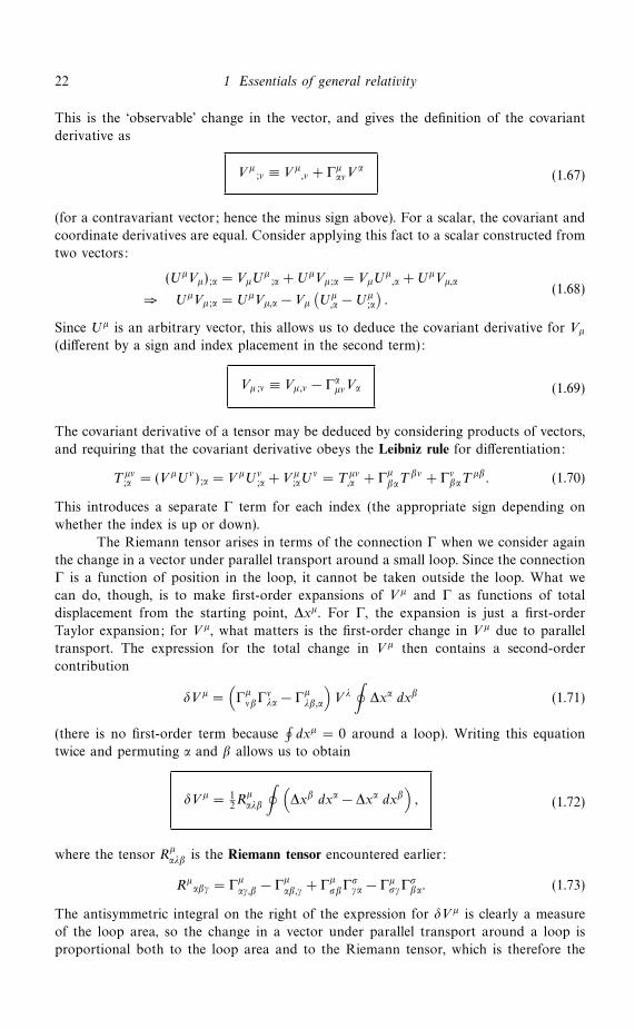
A
BC
Figure 1.2. This figure illustrates the parallel transport of a vectoraround the closed loop ABC on the surface of a sphere. For the case ofthe spherical triangle with all angles equal to 90, the vector rotates by 90in one loop. This failure of vectors to realign under parallel transport isthe fundamental signature of spatial curvature, and is used to define theaffine connection and the Riemann tensor.
the radius of the sphere sample the curvature of the space, and the angular sum starts
to differ from the Euclidean value.
To generalize this process, the concept of parallel transport is introduced. Here,
imagine an observer travelling along some path, carrying with them some vector that
is maintained parallel to itself as the observer moves. This is easy to imagine for small
displacements, where a locally flat tangent frame can be used to apply the Euclidean
concept of parallelism without difficulty. This is clearly a reversible process: a vector can
be carried a large distance and back again along the same path, and will return to its
original state. However, this need not be true in the case of a loop where the observer
returns to the starting point along a different path, as illustrated in figure 1.2. In general,
parallel transport around a loop will cause a change in a vector, and it is this that is the
intrinsic signature of a curved space. We can think of the effect of parallel transport as
producing a change in a vector proportional both to the vector itself (rotation), and to
the distance along the loop (to first order), so that the total change in going once round
a small loop can be written as
δVµ = −∮
Γµαβ V α dxβ. (1.66)
Why the minus sign? The reason for this is apparent when we consider the covariant
derivative of a vector. To differentiate involves taking the limit of [Vµ(x+δx)−Vµ(x)]/δx,
but the difference of Vµ at two different points is not meaningful in the face of general
coordinate transformations. A more sensible procedure is to compare the value of the
vector at the new point with the result of parallel-transporting it from the old point.
22 1 Essentials of general relativity
This is the ‘observable’ change in the vector, and gives the definition of the covariant
derivative as
Vµ;ν ≡ Vµ
,ν + ΓµανV
α(1.67)
(for a contravariant vector; hence the minus sign above). For a scalar, the covariant and
coordinate derivatives are equal. Consider applying this fact to a scalar constructed from
two vectors:
(UµVµ);α = VµUµ;α + UµVµ;α = VµU
µ,α + UµVµ,α
⇒ UµVµ;α = UµVµ,α − Vµ
(Uµ
,α − Uµ;α
).
(1.68)
Since Uµ is an arbitrary vector, this allows us to deduce the covariant derivative for Vµ
(different by a sign and index placement in the second term):
Vµ;ν ≡ Vµ,ν − ΓαµνVα (1.69)
The covariant derivative of a tensor may be deduced by considering products of vectors,
and requiring that the covariant derivative obeys the Leibniz rule for differentiation:
Tµν;α = (VµUν);α = VµUν
;α + Vµ;αU
ν = Tµν,α + Γ
µβαT
βν + ΓνβαT
µβ. (1.70)
This introduces a separate Γ term for each index (the appropriate sign depending on
whether the index is up or down).
The Riemann tensor arises in terms of the connection Γ when we consider again
the change in a vector under parallel transport around a small loop. Since the connection
Γ is a function of position in the loop, it cannot be taken outside the loop. What we
can do, though, is to make first-order expansions of Vµ and Γ as functions of total
displacement from the starting point, ∆xµ. For Γ, the expansion is just a first-order
Taylor expansion; for Vµ, what matters is the first-order change in Vµ due to parallel
transport. The expression for the total change in Vµ then contains a second-order
contribution
δVµ =(ΓµνβΓ
νλα − Γ
µλβ,α
)Vλ
∮∆xα dxβ (1.71)
(there is no first-order term because∮dxµ = 0 around a loop). Writing this equation
twice and permuting α and β allows us to obtain
δVµ = 12R
µαλβ
∮ (∆xβ dxα − ∆xα dxβ
), (1.72)
where the tensor Rµαλβ is the Riemann tensor encountered earlier:
Rµαβγ = Γ
µαγ,β − Γ
µαβ,γ + Γ
µσβΓ
σγα − Γµ
σγΓσβα. (1.73)
The antisymmetric integral on the right of the expression for δVµ is clearly a measure
of the loop area, so the change in a vector under parallel transport around a loop is
proportional both to the loop area and to the Riemann tensor, which is therefore the