COSMIC RAY MEASUREMENTS IN THE ATMOSPHERE

Y.I. Stozhkov, N.S. Svirzhevsky, and V.S. MakhmutovLebedev Physical Institute, Russian Academy of Sciences, Moscow, Russia

AbstractWe present the main characteristics of cosmic ray population in the atmosphereand its variability (11-and 22-year solar cycle variations, solar protonsoriginating from powerful solar flares, energetic electron precipitation duringgeomagnetic disturbances and Forbush decreases of cosmic rays). Theexperimental data were obtained from the long-term cosmic ray monitoring inthe atmosphere from 1957 to now. The relationship between cosmic ray fluxes,and atmospheric processes are also discussed.

1. METHOD OF REGULAR MEASUREMENTS OF COSMIC RAYS IN THE ATMOSPHERE

Regular cosmic ray measurements of cosmic rays are carried out with different instruments: ionizationchambers, meson telescopes, and neutron monitors on the ground. The idea of cosmic ray monitoring inthe atmosphere with radiosondes was suggested by Prof. S.N. Vernov in the middle of fifties and wasrealized by him and Prof. A.N. Charakhchyan in 1957. Now the cosmic ray monitoring cover a wide rangeof cosmic ray energy spectrum. It is schematically shown in Fig. 1.

1

2

3

4

5

7 8 9 1 0 1 1 1 2

lg E, eV

cosm

ic r

ay f

lux

GCR

SCR

nm

atm.

Fig. 1 Schematic view of galactic and solar cosmic ray spectra (GCR, SCR, thick and thin curves accordingly). Thedotted vertical lines show the minimal energy of primary particles, which are detected by radiosondes in theatmosphere (E>0.1 GeV, upper arrow labeled atm) and by neutron monitors on the ground level (E>1.5 GeV, arrowwith nm). The ground-based ionization chambers and meson telescopes record the primary particles with E>9 GeV.

The cosmic ray measurements in the atmosphere are made with standard radiosondes in which thecharged particle detectors are Geiger counter (hereafter counter) and telescope consisting of two countersand with 7 mm Al plate between them. Single counter records charged particles (electrons with energy

E>0.2 MeV, protons with E>5 MeV) and g-rays with E>0.02 MeV (efficiency <1 %). Telescope recordselectrons with E>5 MeV, protons with E>30 MeV and is not sensitive to g-rays. For the isotropic angulardistribution of particles in the upper hemisphere the geometrical factors of these detectors are 15.1 cm2

and 17.8 cm2 sr.

The long-term cosmic ray measurements in the atmosphere have been started at the several latitudeswith the different geomagnetic cutoff rigidities Rc in the middle of the last century and they are continuedtill now [1]. Every day or several times per week balloon flights have been made. Also several seaexpeditions had been organized where the measurements of cosmic ray fluxes in the atmosphere in a widerange of Rc had been made. Till now more than 70.000 balloon flights have been performed. In Table 1the sites and periods of observations are given. The cosmic ray fluxes are measured from the ground levelup to 30-35 km.

Table 1. The sites and periods of cosmic ray measurements in the atmosphere.

Site of observations Geographiccoordinates

Rc, GV Period of observations

Mirny, Antarctica 66∞33¢ S; 93∞00¢ 0.04 03.1963 - present time

Tixie 71∞33¢ N; 128∞54¢ 0.4 02.1978 – 09.1987

Murmansk region 68∞59¢ N; 33∞05¢ 0.6 07.1957 - present time

Norilsk 69∞00¢ N; 88∞00¢ 0.6 11.1974 – 06.1982

Moscow region 55∞28¢ N; 37∞19¢ 2.4 07.1957 - present time

Alma-Ata 43∞12¢ N; 76∞56¢ 6.7 03.1962 – 02.1992

Erevan 40∞10¢ N; 44∞30¢ 7.6 01.1976 – 06.1989

Sea expeditions 60∞ N - 60∞ S 0.1-17 1963-65; 1968-72; 1975-76; 1986-87

In the atmosphere the main part of charged particles is secondary ones except of altitudes h≥20 kmin polar regions where there are low energy primary protons. Below h<20 km cosmic rays mainly consistof secondary electrons and muons.

2. GALACTIC COSMIC RAYS

To study galactic cosmic ray flux variations in different energy intervals the magnetic field of the Earthand the atmosphere are used as separators of charged particles according to their rigidity and energy. Asan example in Fig. 2 the data obtained during the flights of radiosondes at Murmansk, Mirny, and Moscowon September 1997 are presented. During 1997 solar activity level was low and cosmic ray fluxes in theatmosphere were maximal ones.

In Fig. 3 and 4 the samples of data obtained at the northern and southern latitudes with the differentvalues of Rc during the Antarctic sea expedition of 1986-87 are shown [2]. The several radiosondelaunchings were made at the each latitude and averaged data are presented in these figures. One can see anoticeable dependence of cosmic ray fluxes on Rc. Also the atmospheric depth (or pressure) X wheremaximum fluxes of charged particles, Nm, are observed increases with the growth of Rc.

The examples of the time dependencies of charged particle fluxes (monthly averaged values)measured at the polar (northern and southern) and middle latitudes in the stratosphere and troposphere aregiven in Fig. 5 and 6. The period of observations covers ~19-23 solar activity cycles.

Fig. 2. The count rate of single counter vs. altitude in the atmosphere: at the northern polar latitude, Murmanskregion, Rc=0.6 GV (the radiosonde flights on 2 and 4 September 1997 - open circles and black points, accordingly);at Mirny in the Antarctic, Rc=0.04 GV (the flights on 3 and 8 September - open and black triangles, accordingly); atthe middle latitude, Moscow region, Rc=2.4 GV (the flight on 3 September - open squares).

Fig. 3. The cosmic ray fluxes vs. atmospheric pressure X measured at different latitudes of the northern hemisphere during the sea

expedition of 1986-1987. The values of Rc in GV are shown for each curve. The vertical bars show standard errors.

0

5

1 0

1 5

2 0

2 5

3 0

3 5

4 0

0 1000 2000 3000 4000

N, min-1

h, k

m

0.0

0.5

1.0

1.5

2.0

2.5

3.0

3.5

1 10 100 1000

X, g cm-2

N, c

m-2

s-1

0.6

2.4

north

6.7

10.713.7

5.3

Fig. 4. The cosmic ray fluxes vs. atmospheric pressure X measured at different latitudes of the southern hemisphere during the sea

expedition of 1986-1987. The values of Rc in GV are shown for each curve. The vertical bars show standard errors.

From Fig. 6 it is seen that the cosmic ray latitude effect between polar and middle latitudesdisappears in the troposphere that is the cosmic ray fluxes observed at these latitudes are equal.

Fig. 5. Time dependence of monthly averaged cosmic ray fluxes in the stratosphere at h=31 km (X=10 g/cm2) measured at the

northern and southern polar latitudes (Rc=0.6 and 0.04 GV, upper solid and dotted curves, accordingly) and at the middle latitude

(bottom gray curve, Rc=2.4 GV).

0.0

0.5

1.0

1.5

2.0

2.5

3.0

3.5

1 10 100 1000

X, g cm-2

N, c

m-2

s-1

0.04

1.7

2.4

south

3.4

5.47.3

1013.7

1.0

1.5

2.0

2.5

3.0

3.5

5 5 6 5 7 5 8 5 9 5

Year (after 1900)

N, c

m-2

s-1

Fig. 6. Time dependence of cosmic ray fluxes averaged per month in the troposphere at h=10.5 km (X=250 g/cm2) measured at

the northern polar latitudes (Rc=0.6 GV, solid curve) and at the middle latitude (dotted curve, Rc=2.4 GV).

At each atmospheric pressure level, X, g/cm2, only particles with the energy E>Ea (or rigidity R>Ra)where Ea is the atmospheric cutoff energy can contribute to the count rate of our detectors. Theatmospheric cutoff Ea or Ra is defined by the characteristics of nuclear interactions of primary cosmic rayswith air atoms. From the latitude measurements (at the different Rc) one can get the values of atmosphericcutoff as a function of X. In Fig. 7 the relationship of Ra. and X is presented.

0

2

4

6

8

1 0

1 0 100 1000

X, g/cm2

Ra, G

V

Fig. 7. The atmospheric cutoff Ra. vs. atmospheric pressure X. Open points were obtained from the sea expedition data and black

points – from the long-term data obtained at the stationary sites (see Table 1 and Fig, 3, 4). Solid curve is the approximation:

Ra.=0.04X0.8 where R is in GV and X is in g/cm2.

0.7

0.9

1.1

1.3

5 5 6 5 7 5 8 5 9 5

Year (after 1900)

N, c

m-2

s-1

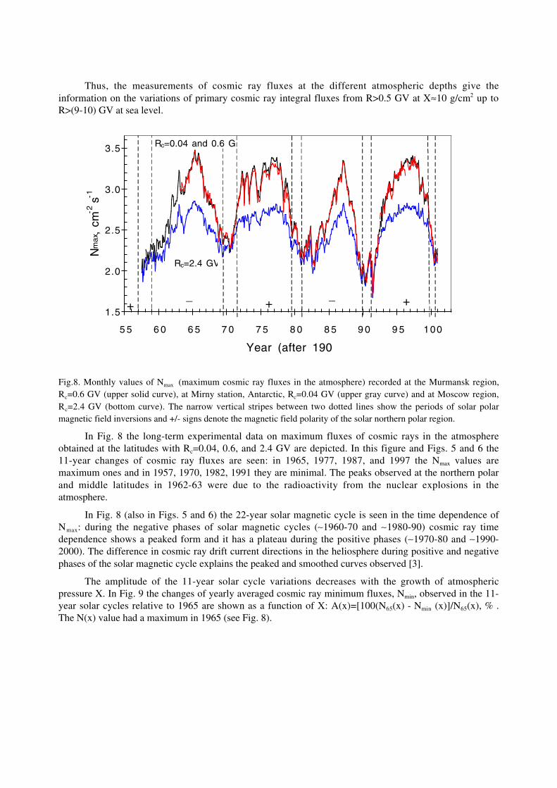
Thus, the measurements of cosmic ray fluxes at the different atmospheric depths give theinformation on the variations of primary cosmic ray integral fluxes from R>0.5 GV at Xª10 g/cm2 up toR>(9-10) GV at sea level.

Fig.8. Monthly values of Nmax (maximum cosmic ray fluxes in the atmosphere) recorded at the Murmansk region,Rc=0.6 GV (upper solid curve), at Mirny station, Antarctic, Rc=0.04 GV (upper gray curve) and at Moscow region,Rc=2.4 GV (bottom curve). The narrow vertical stripes between two dotted lines show the periods of solar polarmagnetic field inversions and +/- signs denote the magnetic field polarity of the solar northern polar region.

In Fig. 8 the long-term experimental data on maximum fluxes of cosmic rays in the atmosphereobtained at the latitudes with Rc=0.04, 0.6, and 2.4 GV are depicted. In this figure and Figs. 5 and 6 the11-year changes of cosmic ray fluxes are seen: in 1965, 1977, 1987, and 1997 the Nmax values aremaximum ones and in 1957, 1970, 1982, 1991 they are minimal. The peaks observed at the northern polarand middle latitudes in 1962-63 were due to the radioactivity from the nuclear explosions in theatmosphere.

In Fig. 8 (also in Figs. 5 and 6) the 22-year solar magnetic cycle is seen in the time dependence ofNmax: during the negative phases of solar magnetic cycles (~1960-70 and ~1980-90) cosmic ray timedependence shows a peaked form and it has a plateau during the positive phases (~1970-80 and ~1990-2000). The difference in cosmic ray drift current directions in the heliosphere during positive and negativephases of the solar magnetic cycle explains the peaked and smoothed curves observed [3].

The amplitude of the 11-year solar cycle variations decreases with the growth of atmosphericpressure X. In Fig. 9 the changes of yearly averaged cosmic ray minimum fluxes, Nmin, observed in the 11-year solar cycles relative to 1965 are shown as a function of X: A(x)=[100(N65(x) - Nmin (x)]/N65(x), % .The N(x) value had a maximum in 1965 (see Fig. 8).

1.5

2.0

2.5

3.0

3.5

5 5 6 0 6 5 7 0 7 5 8 0 8 5 9 0 9 5 100

Year (after 190

Nm

ax,

cm-2

s-1

Rc=2.4 GV

Rc=0.04 and 0.6 G

+ ++__

The value A decreases with the increase of X and at X>600 g/cm2 becomes about 3 %. In June-August, 1991 the absolute minimum cosmic ray fluxes were recorded for the whole period of theobservation from 1957 till present time (see squares in Fig.9)..

Fig. 9. The amplitude of 11-year cosmic ray changes relative to 1965 vs. atmospheric pressure X. The periodsconsidered (months and year) correspond to the minimum cosmic ray fluxes and are given in the insert of this Figure.Cosmic ray fluxes were averaged for these periods. The atmospheric cutoff Ra is shown by solid line.

Fig. 10. Time dependence of maximum cosmic ray flux in the polar atmosphere, Nmax (black curve) and solar activitylevel (gray curve) defined as h/j where h is sunspot number and j is sunspot average helio-altitude. The monthlyaveraged data smoothed with the period of T=3 months were used.

The values of cosmic ray fluxes N(x) in the heliosphere and, in turn, in the atmosphere are definedby solar activity level. The close relationship is observed between N(x) and solar activity parameter (h/j)where h is a sunspot group number, j is sunspot averaged helio-altitude [4]. This relationship isdemonstrated in Fig. 10. The correlation coefficient is R(Nmax, h/j) = –0.83±0.03.

0

10

20

30

40

50

60

0 200 400 600 800

X, g/cm2

A, %

0

1

2

3

4

5

6

7

8

9

Ra ,

(7-9).59(7-9).70(10-12).82(6-8).91

1.5

2

2.5

3

3.5

5 5 6 5 7 5 8 5 9 5

Year (after 190

Nm

ax,

cm-2

s-1

-0.1

0

0.1

0.2

0.3

0.4

0.5

0.6

0.7

0.8

0.9

sola

r ac

tivity

The galactic cosmic ray modulation in the heliosphere is produced by magnetic irregularities ofinterplanetary magnetic field (IMF). In turn, the value of IMF and its irregularity density are defined bysolar activity. The density of these irregularities increases with the growth of IMF strength. So, we canexpect a relationship between IMF strength and cosmic ray fluxes in the heliosphere as well as in theatmosphere. This relationship is given in Fig. 11. The correlation coefficient R(Nmax, IMF)= -0.71±0.04.

Fig.11. Time dependence of maximum cosmic ray flux in the polar atmosphere, Nmax (black curve) and IMF (graycurve). The monthly averaged data smoothed with the period of T=3 months were used. The data on IMF were takenfrom INTERNET: http://nssdc.gsfc.nasa.gov/omniweb/.

Fig. 12. Cosmic ray fluxes recorded in the atmosphere at Mirny in the Antarctic during the solar proton event on 9November 2000. Solid curve is a charged particle flux background produced by galactic cosmic rays in theatmosphere (GCR). Different symbols show the data obtained during the different flights of radiosondes (the dateand start time of launchings are given in the insert)..

1.5

2

2.5

3

3.5

5 5 6 5 7 5 8 5 9 5

Year (after 190

Nm

ax,

cm-2

s-1

4

5

6

7

8

9

1 0

1 1

IMF,

0

5

1 0

1 5

2 0

2 5

3 0

0.1 1.0 10.0 100.0

N, cm-2 s-1

h, k

m

GCR

0822 11.09.0

1053 11.09.0

1942 11.09.0

0326 11.10.0

Start time, UT, date

3. SOLAR COSMIC RAYS, PRECIPITATION, AND RADIOACTIVITY

Since the beginning of cosmic ray measurements in the atmosphere in 1957 several tens of solar protonevents were recorded (e.g. [5]). As a rule such events are observed in the polar atmosphere where Rc arerather low (see Table 1). During solar proton events total cosmic ray flux at high altitudes in theatmosphere increases in several (sometimes in tens) times. As example, the solar proton fluxes generatedby solar flare on November 9, 2000 and recorded in the Earth’s atmosphere are given in Fig. 12. Solarproton fluxes were observed in the atmosphere at h>17 km and their values increase with altitude.

Fig. 13. The energy spectra of solar protons on 9 November 2000. The start times of radiosonde launchings andexponents g of solar proton energy spectra I(>E)~E-g are given below: 1 –Date - 11.09.00, Start time (UT) - 8:22,g=7.2; 2 – Date - 11.09.00, Start time (UT) - 10:53, g=5.8; 3 – Date - 11.09.00, Start time (UT) - 13:36, g=7.8; 4 –Date – 11.10.00, Start time (UT) - 19:42, g=4.9.

From these data the fluxes and energy spectra of solar flare particles in the energy range of E=100-500 MeV were obtained. They are depicted in Fig. 13. In this solar proton event the particles with E>500MeV were not observed and this event was not recorded by neutron monitors. We note that the observedsolar proton “soft” energy spectra could be due to the additional acceleration of particles in theinterplanetary space by shock waves as it was happened in the past during the solar proton events inAugust 1972 [6].

Fig. 14. The time dependences of yearly number of the solar proton events recorded in the atmosphere (black pointsand right axes) and yearly sunspot number (open points and left axes).

0.1

1

1 0

100

100 1000

E, MeV

J(>E

), cm

-2 s

-1 s

r-1

1

2

3

4

0

5 0

100

150

200

1955 1965 1975 1985 1995

Year

suns

pot n

umbe

r

0

2

4

6

8

1 0

sola

r pr

oton

eve

nt n

umbe

r

For the 45-year period of cosmic ray monitoring in the atmosphere 105 solar proton events wererecorded. In Fig. 14 the time dependence of the yearly number of these events and solar activity level(sunspot number) are shown. It is seen that the solar proton events mainly occur during the ascending anddescending phases of solar activity.

0

5

1 0

1 5

2 0

2 5

3 0

3 5

0 1 2 3 4

N, cm-2 s-1

h, k

m

1250 05.03.0

0930 05.05.0

Start time UT Date

0

5

1 0

1 5

2 0

2 5

3 0

3 5

0 1 2 3

N, cm-2 s-1h,

km

1250 05.03.0

0930 05.05.0

Start time UT Date

Fig. 15. Precipitation of high energy electrons into the northern polar atmosphere recorded by single counter on 5March 2000 (left panel, black points). The background from galactic cosmic rays is shown by open points. Thetelescope recorded galactic cosmic ray background only (right panel). The inserts show the dates of radiosondeflights and launching times.

During the geomagnetic disturbed periods in the polar atmosphere at high altitudes high-energyelectron precipitation events are detected [7, 8, 9]. Our northern polar station in Murmansk region is nearthe polar oval (McIlwain’s parameter L=5.6) where the precipitations are observed rather often. In Fig. 15the example of precipitation detected on November 2000 is shown. The counter records secondary g-raysproduced by precipitating electrons in the atmosphere..

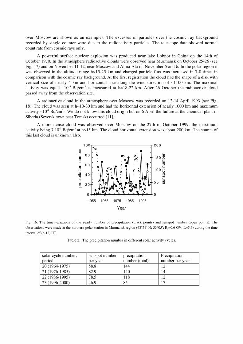
But at the same time the telescope records only the background from galactic cosmic rays and itallows to separate precipitation from solar proton events. It is significant that g-rays recorded in theatmosphere at h=25-35 km are produced by the precipitating electrons with E>several MeV. The timedependence of the yearly precipitation number and the sunspot number are given in Fig. 16. Into theprecipitation data the corrections for patrol efficiency were introduced. The data obtained show that theprecipitation take place most often during the descending phase of solar activity (remind that solar protonevents are observed most often during the ascending and descending solar activity phases, see Fig. 14).This fact was established earlier in other papers [10]. The total number of precipitation recorded at thestation in Murmansk region during 1957-2000 equals 549 events. For almost the same period (1963-2000)at the Antarctic station Mirny (66∞33 ¢ S; 93∞00¢; Rc=0.04 GV; Lª11) 10 precipitation events wererecorded only.

In Table 2 the yearly precipitation numbers for 20 - 23rd solar cycles are given. The last line in thisTable includes the ascending phase of 23rd solar activity cycle only.

The regular monitoring of charged particle fluxes in the atmosphere provides the prompt control ofradiation conditions and allows to detect radiation clouds from nuclear explosions or nuclear plantfailures. In Fig. 17 and 18 the observations of radioactive clouds in the polar northern atmosphere and

over Moscow are shown as an examples. The excesses of particles over the cosmic ray backgroundrecorded by single counter were due to the radioactivity particles. The telescope data showed normalcount rate from cosmic rays only.

A powerful surface nuclear explosion was produced near lake Lobnor in China on the 14th ofOctober 1970. In the atmosphere radioactive clouds were observed near Murmansk on October 25-26 (seeFig. 17) and on November 11-12, near Moscow and Alma-Ata on November 5 and 6. In the polar region itwas observed in the altitude range hª15-25 km and charged particle flux was increased in 7-8 times incomparison with the cosmic ray background. At the first registration the cloud had the shape of a disk withvertical size of nearly 4 km and horizontal size along the wind direction of ~1100 km. The maximalactivity was equal ~10-3 Bq/cm3 as measured at hª18-22 km. After 26 October the radioactive cloudpassed away from the observation site.

A radioactive cloud in the atmosphere over Moscow was recorded on 12-14 April 1993 (see Fig.18). The cloud was seen at hª10-30 km and had the horizontal extension of nearly 1000 km and maximumactivity ~10-4 Bq/cm3. We do not know this cloud origin but on 6 April the failure at the chemical plant inSiberia (Seversk town near Tomsk) occurred [11].

A more dense cloud was observed over Moscow on the 27th of October 1999, the maximumactivity being 7◊10-3 Bq/cm3 at h>15 km. The cloud horizontal extension was about 200 km. The source ofthis last cloud is unknown also.

Fig. 16. The time variations of the yearly number of precipitation (black points) and sunspot number (open points). The

observations were made at the northern polar station in Murmansk region (68∞59¢ N; 33∞05¢; Rc=0.6 GV; L=5.6) during the time

interval of (6-12) UT.

Table 2. The precipitation number in different solar activity cycles.

solar cycle number,period

sunspot numberper year

precipitationnumber (total)

Precipitationnumber per year

20 (1964-1975) 58.8 144 1221 (1976-1985) 82.9 140 1422 (1986-1995) 78.5 118 1223 (1996-2000) 46.9 85 17

0

2 0

4 0

6 0

8 0

100

1955 1965 1975 1985 1995

Year

prec

ipita

tion

num

ber

0

5 0

100

150

200

suns

pot

num

ber

Fig. 17. Charged particle fluxes in the northern polar atmosphere detected by single counter. At h>15 km the excessof flux over the cosmic ray background (solid gray line) is due to radioactive cloud particles produced by the nuclearexplosion in China on 14 October 1970. In the insert the legend on the balloon start time is given.

Fig. 18. The count rate of single counter vs. altitude in the atmosphere over Moscow on 12-14 April 1993:æbackground from galactic cosmic rays; charge particle flux measurements on 13 April, launching local time 0830 LT(◊), on 13 April, 1430 LT (D); on 14 April, 0830 LT ( );.

4. COSMIC RAY FLUXES AND ATMOSPHERIC PROCESSES

If one compares the flux of solar electromagnetic radiation falling on the top of the atmosphere (Fsunª1010

erg m-2 s-1) with the flux of cosmic ray energy (FCRª102 erg m-2 s-1 for particles with energy E≥0.1 GeV)the evident conclusion could be made: the influence of charged cosmic ray particles on the processes inthe atmosphere is negligible in comparison with influence of the electromagnetic radiation coming fromthe Sun. However, let us imagine for a moment that cosmic rays stopped to intrude into the Earth’satmosphere. The ion production will be aborted and the global electric circuit will be destroyed. Theproduction of thundercloud electricity and lightning will be over. The cloud area will be decreased andprecipitation level will fall down.

0

5

1 0

1 5

2 0

2 5

3 0

0 5 1 0 1 5 2 0

N, cm-2

s-1

h, k

mbackground1602 LT 25 Oct. 1971802 LT 25 Oct. 1972207 LT 25 Oct. 1971157 LT 26 Oct. 197

0

10

20

30

40

0 1 2 3 4 5

N, cm-2 s-1

h, k

m

The cosmic rays with energy E=0.1-15 GeV carry about 60 % of all cosmic ray energy and theseparticles constitute about 95 % of all cosmic ray flux. These particles undergo the influence of thegeomagnetic field in such way that the fluxes of primary cosmic rays at polar latitudes is higher than theones at equatorial regions as much as ~30-35 times. In the atmosphere this difference is about 4 times.

Below some aspects of influence of charged particle fluxes on atmospheric processes areconsidered (see also [12]). In our analysis we use the experimental data of the long-term measurements ofcosmic ray fluxes at the different atmospheric depths (from the Earth’s surface up to 30-35 km) and at thedifferent latitudes.

4.1 The global electric circuit and ion production

It is well known that the Earth has a negative electric charge about 6¥105 C and the strength of electricfield produced by this charge near the Earth’s surface measured during fair-well weather equals Eª-130V/m (directed to the Earth’s surface). The value of average current flowing between equalizing layer to bein the ionosphere at the altitude hª55-80 km and the Earth’s surface is Iª10-12A/m2 [13, 14]. The light ionsprovide this current in the atmosphere. The ions are produced by cosmic particles (radioactivity of soilalso gives ions but only in the lower atmosphere at h< 3 km). If cosmic ray flux changes the ion densitythe air conductivity changes also. The lightning in thunderstorms and precipitation form another branch ofthe closed electric circuit charging the Earth by negative electricity and providing electric current from theEarth to the ionosphere. The sketch of global electric circuit is given in Fig. 19 (see, e.g. [16]).

Earth

h =60 kmIpRp

Ig

Im, Rm

Fig. 19. The sketch of the global electric circuit: h=60 km – equalizing layer; Ip, Rp and Im, Rm – atmospheric electriccurrents and resistances in the atmosphere at polar and middle latitudes, accordingly; Ig – current of thunderstormsand precipitation charging the Earth by negative electricity.

The equation describing the relation between ion production rate, q, and their recombination in theatmosphere under quasi-state conditions is usually taken in the form

q(h)=a(h) [n(h)]2, (1)

where n is ion concentration, a is recombination coefficient, h is atmospheric altitude [17]. Using theexperimental data on cosmic ray fluxes and ion concentrations in the atmosphere one can test the validityof this equation. In Fig. 20 the ion concentrations, n, and the charged particle fluxes, N, measured atseveral latitudes vs. altitude are presented [18]. From the experimental data on ion concentration n andcosmic ray flux N one can get that the ion production rate q is proportional to charged particle flux:q(h)=msN(h), where m and s are the number of air particles per cm3 and ionization cross-section. Thevalues of m and s are the same for different latitudes and depends on the altitude only. It isn’t true for thecase of polar latitudes and h>20 km where s is increased. At h<20 km the value of s equals 2*1018 cm2

within 10-15 % for all latitudes.

0

10

20

30

0 1 2 3

n, 103 cm-3

h, k

m17.3 5.3

30.6

0

10

20

30

0 1 2

N, cm-2 s-1

h, k

m

17.3 5.6 3.4 0.04

Fig. 20. Ion concentration n (left panel) and cosmic ray flux N (right panel) as a functions of altitude h in theatmosphere at the latitudes with the geomagnetic cutoff rigidities Rc=17.3, 5.6, 5.3, 3.0, 3.4, 0.6 and 0.04 GV.Horizontal bars show the standard errors.

Let us consider the measurements of n and N performed at two different latitudes. According to theexpression (1), we can construct the following ratio:

[q1(h)/q2(h)]=[a(h) n2(h)]1/[a(h) n2(h)]2, (2)

where the subscripts 1 and 2 correspond to the latitudes with different geomagnetic cutoff rigidities Rc1 andRc2. Substituting msN(h) instead of q and taking (ms)1= (ms)2 and a1ªa2 (these suggestions are fulfilledin the atmosphere rather well) one can get

[N1(h)/N2(h)]=[n1(h)/n2(h)]2. (3)

0.0

0.2

0.4

0.6

0.8

5 10 15 20 25 30

h, km

Rat

io

1

2

3

Fig. 21. The ratio of cosmic ray fluxes (curve 1), ion concentrations (curve 2) and squared ion concentrations (curve3) as a function of altitude. These values were calculated from the experimental data obtained at the equatorial(Rc=17.3 GV) and middle (Rc=3.3 GV) latitudes (see Fig.20) without any normalization of the data. The standarderrors are given by vertical bars.

In Fig. 21 the ratios of charged particle fluxes (curve 1-open points), ion concentrations (curve 2-dark points), and squared ion concentrations (curve 3-crosses) obtained from the experimental datapresented in Fig. 20 are given. The data obtained in the equatorial (Rc=17.3 GV) and middle latitudes(Rc=3.3 GV) were used.

It is seen that the ratio of cosmic ray fluxes (curve 1) coincides with ion concentration one (curve 2)and differs significantly from squared ion concentration ratio (curve 3). The details of such considerationare given in [18]. Thus, from this analysis the important conclusion must be made that the ion balance inthe atmosphere under quiet conditions is described by linear equation (not quadratic one)

q(h)=b(h) n(h), (4)

where b(h) is the linear recombination coefficient. From the available experimental data on cosmic rays inthe atmosphere and light ion concentrations the value of b(h) and q(h) can be calculated for any site of theEarth and any level of solar activity.

The ion production rate q can be written as

q(h)=N(h) s(h) r(h)/M, (5)

where N(h) is cosmic ray flux at the altitude h, s is the ionization cross-section in air, r(h) is the airdensity and M is the average mass of air atom. The relationship between atmospheric electric current J,electric field strength E and conductivity l is

J=l(h) E(h)=n(h) k(h) E(h), (6)

where k(h) is the mobility of light ions at the altitude h. Thus, using the expressions 4, 5 and 6 one canfind

J=N(h) s(h) r(h) k(h) E(h)/[M b(h)]. (7)

0.8

1.2

1.6

2

1 9 6 5 1 9 7 0 1 9 7 5 1 9 8 0 1 9 8 5Year

J, 1

0-12 A

m-2

0.54

0.58

0.62

0.66

N, c

m-2

s-1

J

N

Fig. 22. The yearly average values of atmospheric electric current J(h) (from [19]) and cosmic ray flux N(h) at hª8km in the polar region.

On the right side of this equation all values are constant except cosmic ray flux N(h) and electricfield strength E(h). If one supposes that E(h) is constant or weakly changes in the periods of fair-wellweather then there is the linear relationship of cosmic ray flux N(h) and atmospheric electric current J(h).Such conclusion is confirmed by the experimental data showed in Fig.22. The data on J(h) were takenfrom [19]. The correlation coefficient between J(h) and N(h) is positive and equals r(J, N)= +0.77±0.10.The correlation of atmospheric electric current and solar activity level (sunspot number W) is low,r(J,W)=-0.32±0.22.

4.2 Thundercloud electricity and lightning production

In 1920 Wilson put forward fascinating idea suggested that thunderstorms act as a global generator ofelectric current maintaining the Earth’s electric charge [20]. Since the experimental evidences supportingthis hypothesis were obtained (see references in [14]). However, the mechanisms of thunderstormelectricity production (separation of negative and positive charges in thundercloud) and lightninggeneration are not clear till present time, although there are a number of hypotheses on the thundercloudelectricity origin (see, e.g., [21-23]). Cosmic rays could be responsible for the thunderstorm electrification[24].

Secondary charged particle fluxes generated in the atmosphere by primary cosmic rays are the onlysource of positive and negative ion production in the atmosphere at h>(2-3) km. The problem consists inthe spatial separation of negative and positive ions in the process of thundercloud formation. Thethunderclouds are formed from ascending wet air mass when the fronts of cold and warm air meet eachother. The air masses contain heavy ions (charged aerosols) because light ions produced by cosmic raysadhere to neutral heavy particles. As it is known from the observations the concentration of aerosols has amaximum in the low atmosphere near the Earth’s surface and its value is ~2¥104 cm-3. The half of theseparticles carries out the positive or negative electric charges [25]. Ascending air mass picks up theaerosols. During ascending air mass is cooled and processes of condensation of water molecules onneutral and charged aerosols take place. The condensation rate depends essentially on the charge presenceand its sign. Namely, negative charged aerosols grow faster than positive ones as much as ~104 times [26,27]. The rapid growth of aerosols with negative charge makes them heavy and their lift with the rising airmass is stopped at the low altitudes. At the same time aerosols with positive charge continue to rise withascending wet air mass and stop their rising at higher altitudes than negative charged aerosols. In this waythe spatial separation of electric charges inside the cloud occurs (in detail see [24]).

Inside the thundercloud the strength of electric field can grow up to Eª3 kV/cm and the distancebetween separated positive and negative charges is roughly estimated as Dhª3-4 km. The high value of Eis observed under thundercloud also. But the observed values of E are much less than the puncture voltageat the altitudes where thunderclouds exist (hª2-7 km). At hª3 km the value of puncture voltage is 15-30kV/cm [28]. In [29] Ermakov put forward the idea that in such electric fields the discharges (lightning) areproduced by extensive air showers arising from high energy cosmic ray particles with e =1014-10 15 eV.These high-energy cosmic rays interact with nuclei of ambient air and give rise to many thousands ofcharged secondaries. Along ionized tracks of these secondary particles in a strong electric field theavalanches develop and propagate. The high energy cosmic ray particle flux is enough to explain thenumber of lightning observed. As cosmic rays hit the Earth’s atmosphere accidentally in all directions thelightning arise by chance also. There is another mechanism of lightning production suggested by Gurevich[30, 31] in which relativistic electron is accelerated in the electric field of thundercloud and producesavalanche.

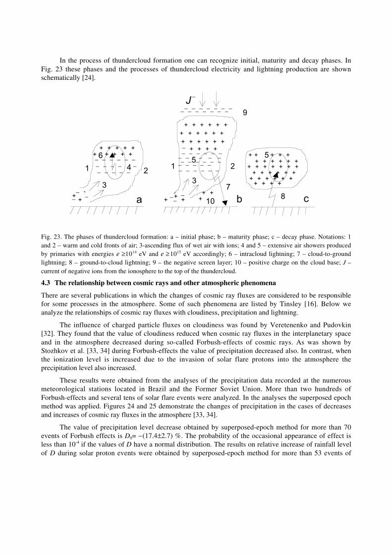
In the process of thundercloud formation one can recognize initial, maturity and decay phases. InFig. 23 these phases and the processes of thundercloud electricity and lightning production are shownschematically [24].

_ _ _ _ _ _ _ _ _ _ _ _ _ _

_ _ _ _ _ __ _ _ _ _ _

+ + + + + ++ + + + +

+ + + + + +

_ _ _ _ _

+ + + +

+

_

1 12 2

3 3

+ + + + + + + + + + +

+ + + + + + ++ + + + + +

+ + + + + ++ + + +

+ _+_+

_ + ++

++

__+_

+ + + + +_ _ _ _ _ __ _ _ _ _

9

a b c87

55

4 _ _ _ _ _ __ _ _ _ _

10

6

J_

+ + + + + _ _ _ _ _

Fig. 23. The phases of thundercloud formation: a – initial phase; b – maturity phase; c – decay phase. Notations: 1and 2 – warm and cold fronts of air; 3-ascending flux of wet air with ions; 4 and 5 – extensive air showers producedby primaries with energies e ≥1014 eV and e ≥1015 eV accordingly; 6 – intracloud lightning; 7 – cloud-to-groundlightning; 8 – ground-to-cloud lightning; 9 – the negative screen layer; 10 – positive charge on the cloud base; J –current of negative ions from the ionosphere to the top of the thundercloud.

4.3 The relationship between cosmic rays and other atmospheric phenomena

There are several publications in which the changes of cosmic ray fluxes are considered to be responsiblefor some processes in the atmosphere. Some of such phenomena are listed by Tinsley [16]. Below weanalyze the relationships of cosmic ray fluxes with cloudiness, precipitation and lightning.

The influence of charged particle fluxes on cloudiness was found by Veretenenko and Pudovkin[32]. They found that the value of cloudiness reduced when cosmic ray fluxes in the interplanetary spaceand in the atmosphere decreased during so-called Forbush-effects of cosmic rays. As was shown byStozhkov et al. [33, 34] during Forbush-effects the value of precipitation decreased also. In contrast, whenthe ionization level is increased due to the invasion of solar flare protons into the atmosphere theprecipitation level also increased.

These results were obtained from the analyses of the precipitation data recorded at the numerousmeteorological stations located in Brazil and the Former Soviet Union. More than two hundreds ofForbush-effects and several tens of solar flare events were analyzed. In the analyses the superposed epochmethod was applied. Figures 24 and 25 demonstrate the changes of precipitation in the cases of decreasesand increases of cosmic ray fluxes in the atmosphere [33, 34].

The value of precipitation level decrease obtained by superposed-epoch method for more than 70events of Forbush effects is D0= -(17.4±2.7) %. The probability of the occasional appearance of effect isless than 10-4 if the values of D have a normal distribution. The results on relative increase of rainfall levelof D during solar proton events were obtained by superposed-epoch method for more than 53 events of

solar proton enhancements. The amplitude of positive increase is D0=(13.3±5.3) %. The probability ofeffect appearance by chance is less than 10-2.

-20

-15

-10

-5

0

5

1 0

-35 -25 -15 -5 5 1 5 2 5 3 5

D, %

Days

Fig. 24. The changes of the daily precipitation level, D, %, relative to mean value evaluated from precipitation dataduring 1 month before (-30 to –1 days) and 1 month after (1 to 30 days) Forbush decrease event. The day “0”correspond to the Forbush decrease main phase. The precipitation data used in the analyses were obtained in theFormer Soviet Union and Brazil.

-15

-10

-5

0

5

10

15

-30 -20 -10 0 10 20 30Day

D, %

Fig. 25. The changes of the daily precipitation level, D, %, relative to mean value evaluated from precipitation dataduring 1 month before and 1 month after solar proton events recorded by ground-based neutron monitors (“0”-day).

The link of cosmic ray intensity and global cloud coverage was found by Svensmark and Friis-Christensen [35]. Their results demonstrate the relationship between charged particle fluxes on the Earth’s

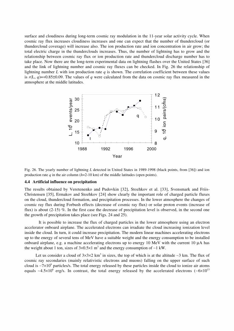
surface and cloudiness during long-term cosmic ray modulation in the 11-year solar activity cycle. Whencosmic ray flux increases cloudiness increases and one can expect that the number of thundercloud (orthundercloud coverage) will increase also. The ion production rate and ion concentration in air grow; thetotal electric charge in the thunderclouds increases. Thus, the number of lightning has to grow and therelationship between cosmic ray flux or ion production rate and thundercloud discharge number has totake place. Now there are the long-term experimental data on lightning flashes over the United States [36]and the link of lightning number and cosmic ray fluxes can be checked. In Fig. 26 the relationship oflightning number L with ion production rate q is shown. The correlation coefficient between these valuesis r(L, q)=+0.85±0.09. The values of q were calculated from the data on cosmic ray flux measured in theatmosphere at the middle latitudes.

10

15

20

25

30

1988 1992 1996 2000

Year

L, 1

06 e

ven

ts/y

ea

r

8

9

10

11

12

q, 1

06 ion

pai

rs/(

cm2 s

)

L

q

Fig. 26. The yearly number of lightning L detected in United States in 1989-1998 (black points, from [36]) and ionproduction rate q in the air column (h=2-10 km) of the middle latitudes (open points).

4.4 Artificial influence on precipitation

The results obtained by Veretenenko and Pudovkin [32], Stozhkov et al. [33], Svensmark and Friis-Christensen [35], Ermakov and Stozhkov [24] show clearly the important role of charged particle fluxeson the cloud, thundercloud formation, and precipitation processes. In the lower atmosphere the changes ofcosmic ray flux during Forbush effects (decrease of cosmic ray flux) or solar proton events (increase offlux) is about (2-15) %. In the first case the decrease of precipitation level is observed, in the second onethe growth of precipitation takes place (see Figs. 24 and 25).

It is possible to increase the flux of charged particles in the lower atmosphere using an electronaccelerator onboard airplane. The accelerated electrons can irradiate the cloud increasing ionization levelinside the cloud. In turn, it could increase precipitation. The modern linear machines accelerating electronsup to the energy of several tens of MeV have a suitable weight and the energy consumption to be installedonboard airplane, e.g. a machine accelerating electrons up to energy 10 MeV with the current 10 mA hasthe weight about 1 ton, sizes of 3¥0.5¥1 m3 and the energy consumption of ~1 kW.

Let us consider a cloud of 3¥3¥2 km3 in sizes, the top of which is at the altitude ~3 km. The flux ofcosmic ray secondaries (mainly relativistic electrons and muons) falling on the upper surface of suchcloud is ~7¥109 particles/s. The total energy released by these particles inside the cloud to ionize air atomsequals ~4.5¥106 erg/s. In contrast, the total energy released by the accelerated electrons (~6¥1013

electrons/s) is ~109 erg/s. Thus, the accelerator with the parameters given above could increase theionization inside the cloud in 10-100 times in comparison with the natural background produced bycosmic rays.

In comparison with the methods of artificial influence on the clouds used in practice [37, 38] theirradiation of clouds by accelerated particles is safe because the accelerated electrons and their secondarieswill be absorbed in ambient air because of its energy losses. The proposed method could be useful tostruggle with droughts and downpours causing floods.

5. CONCLUSION

We present the main characteristics of cosmic ray population in the atmosphere and its variability. Theexperimental data were obtained from the long-term cosmic ray monitoring in the atmosphere from 1957to now. The main features of cosmic ray variability are the following:

• 11-and 22-year solar cycle variations;

• solar proton events originating from powerful solar flares;

• energetic electron precipitation during geomagnetic disturbances and Forbush decreases of cosmicrays;

The cosmic ray monitoring in the atmosphere allows to detect radioactive clouds producing bynuclear explosions or failures at atomic plants.

Cosmic ray particle fluxes play important role in many atmospheric processes and only now thisrole begins to be elucidated. The thundercloud electricity and lightning production, cloud formation,influence on the value of global cloudiness and precipitation on the short (days) and long (11-year solaractivity cycle) time scales, operation of global electric circuit and long-scale global climate changesdepend on the values of cosmic ray flux.

ACKNOWLEDGEMENTS

We are very grateful to our colleagues who made hard work to get the experimental data on the long-termcosmic ray variations in the atmosphere. This work is partly supported by Russian Foundation for BasicResearch (grants No. 01-02-31005 and No. 99-02-18222).

REFERENCES

[1] A.N. Charakhchyan, G.A. Bazilevskaya, Y.I. Stozhkov, and T.N. Charakchyan, Cosmic rays inthe atmosphere and in space near the Earth during 19 and 20 solar activity cycles, Tr. Fis. Inst. imP.N. Lebedeva, Russian Akad. Nauk, Nauka, 83 (1976) 3 (in Russian).

[2] A.E. Golenkov , A.K. Svirzhevskaya, N.S. Svirzhevsky, and Y.I. Stozhkov, Cosmic ray latitudesurvey in the stratosphere during the 1987 solar minimum, Conf. Pap., Int. Cosmic Ray Conf.,XXIst, 7 (1990) 14.

[3] H. Moraal, Observations of the eleven-year cosmic-ray modulation cycle, Space Sci. Rev., 19(1999) 845.

[4] Y.I. Stozhkov and T.N. Charakhchyan, On the role of the heliolatitudes of the sunspots in the 11-year galactic cosmic ray modulation, Acta Physics Academial Sciantiarum Hungaricae, (Suppl.2), 29 (1970).

[5] G.A. Bazilevskaya, M.B. Krainev, Yu.I. Stozhkov , A.K. Svirzhevskay, and N.S. Svirzhevsky,Long-term Soviet program for the measurement of ionizing radiation in the atmosphere, Journ.Geomag. and Geoelectr., 43 (1991) 893.

[6] G.A. Bazilevskaya., A.N. Charakhchyan, Y.I. Stozhkov, and T.N. Charakhchyan, The energyspectrum and the conditions of propagation in the interplanetary space for solar protons during thecosmic ray events on August 4 to 9, 1972, Conf. Pap., Int. Cosmic Ray Conf., XIIIrd, Denver,USA, 2 (1973).

[7] V.S Makhmutov, G.A. Bazilevskaya, A.I. Podgorny, Y.I. Stozhkov, and N.S. Svirzhevsky, Theprecipitation of electrons into the Earth's atmosphere during 1994, Proc. 24 ICRC, Italy, Rome, 4(1995) 1114.

[8] G.A. Bazilevskaya and V.S. Makhmutov, The electron precipitation into the atmosphereaccording to cosmic ray experiment in the stratosphere, Izv. AN SSSR, Ser. Fiz., 63 (1999) 1670(in Russian).

[9] V.S. Makhmutov, G.A. Bazilevskaya, M.B. Krainev, Characteristics of energetic electronrecipitation into the Earth's polar atmosphere and geomagnetic conditions, Adv. Space. Res.,(2001) (in press).

[10] G.D. Reeves, Relativistic electrons and magnetic storms: 1992-1995, Geoph. Res. Lett., 25 (1998)1817.

[11] G.A. Bazilevskaya, A.K. Svirzhevskay, N.S. Svirzhevsky, Y.I. Stozhkov, Radioactive cloud inthe atmosphere at Moscow site on 12-14 April 1993, Kratkie soobsheniya po fizike, Moscow,Lebedev Instituite, 7-8 (1994) 36 (in Russian).

[12] Y.I. Stozhkov, V.I. Ermakov, and P.E. Pokrevsky, Cosmic rays and atmospheric processes, Izv.Russian Akad. Nauk, ser. fiz., 65 (2001) 406 (in Russian).

[13] J. Alan Chalmers, Atmospheric Electricity, Pergamon press (1967).

[14] R. Reiter, Phenomena in Atmosphere and Environmental Electricity, Amsterdam, Elsvier (1992).

[15] R. Markson, Solar modulation of atmospheric electrification and possible implications for theSun-Weather relationship, Nature, 273 (1978) 103.

[16] Brain A. Tinsley, Correlations of atmospheric dynamics with solar wind-induced changes of air-earth current density into cloud tops, Journ. Geophys. Res., 101 (1996) 29,701.

[17] L.B. Loeb, Basic Processes of Gaseous electronics, New-York (1960).

[18] V.I. Ermakov, G.A. Bazilevskaya, P.E. Pokrevsky, and Y.I. Stozhkov. Ion balance equation inthe atmosphere, Journ. Geoph. Res., 102 (1997) 23,413.

[19] R.G. Roble, On solar-terrestrial relationships in the atmospheric electricity, Journ. Geoph. Res.,90 (1985) 6000.

[20] C.T. Wilson, The maintenance of the Earth's electric charge, Observatory, 45 (1922).

[21] E.R. Williams, Electricity of thunderclouds, Scientific American, 1 (1989) 34.

[22] M.B. Baker and J.G. Dash, Mechanism of charge transfer between colliding ice particle inthunderstorms, Journ. Geoph. Res., 99 (1994) 10,621.

[23] V. Brooks, C.P.R. Saunders, An experimental investigation of the inductive mechanism ofthundercloud electrification, Journ. Geoph. Res., 99 (1994) 10,627.

[24] V.I. Ermakov and Y.I. Stozhkov, New mechanism of thundercloud electricity and lightningproduction, Proc. 11-th Intern. Conf. Atmospher. Elect., Alabama, USA (1999) 242.

[25] P.N. Tverscoi, , Course of meteorology, Leningrad, Gidrometeoizdat, (1962) (in Russian).

[26] A.I. Rusanov and V.L. Kusmin, On the influence of electric field on the surface tension of thepolar liquid, Kolloidnyi Journal, 39 (1977) 388 (in Russian).

[27] A.I. Rusanov, To thermodynamics of nucleation on charged centers, Doklady Academii Nauk,USSR, 238 (1978) 831 (in Russian).

[28] J.M. Meek and J. Craggs, Electrical Breakdown of Gases, Oxford, the Claredon Press (1953).

[29] Ermakov , Molnii-sledy chastiz sverchvysokich energii, Nayka I zhizn, Moskva, Prosveshenie(1993) 92 (in Russian).

[30] A.V. Gurevich , G.M. Molikh, and R.A. Roussel-Dupre, Runaway mechanism of air breakdownand preconditioning during a thunderstorm, Phys. Lett., A, 165 (1992) 463.

[31] A.V. Gurevich, K.P. Zubin, R.A. Roussel-Dupre, Lightning initiation by simultaneous effect ofrunaway breakdown and cosmic ray showers, Phys. Lett., A, 254 (1999) 79.

[32] S.V. Veretenenko and M.I. Pudovkin, Effects of forbush-decreases in cloudiness variations,Geomagn. and Aeronomy, 34 (1994) 38 (in Russian).

[33] Y.I. Stozhkov , J. Zullo, Jr., I.M. Martin, G.Q. Pellegrino, H.S. Pinto, P.C. Bezerra, G.A.Bazilevskaya, V.S. Machmutov, N.S. Svirzevskii, A. Turtelli, Jr., Rainfalls during greatForbush-decreases, Nuovo Cimento, 18C (1995) 335.

[34] Y.I. Stozhkov , P.E. Pokrevsky, J. Zullo, Jr., I.M. Martin, V.P. Ohlopkov, G.Q. Pellegrino,H.S. Pinto, P.C. Bezerra, A. Turtelli, Jr., Influence of charged particle fluxes on precipitation,Geomagn. and Aeronomy, 36 (1996) 211 (in Russian).

[35] H. Svensmark and E. Friis-Christensen, Variation of cosmic ray flux and global coverage - amissing link in solar-climate relationships, Journ. Atmospheric and Solar-Terrest. Physics, 59(1997) 1225.

[36] R.E. Orville, G.R. Huffines, Lightning ground flash measurements over contiguous United States:a ten-year summary 1989-1998, Proc. 11th Intern. Conf. Atmospher. Electr., Alabama, USA,(1999) 412.

[37] L.G. Kachurin, Fisicheskie osnovy vosdeistviya na atmosfernye processy, Gidrometeoisdat,Leningrad (1990) (in Russian).

[38] New Scientist, New method of production artificial precipitation, 151 (1996) 10.