corrosion induced failures of prestressing steel ... · corrosion induced failures of prestressing...
TRANSCRIPT
Corrosion induced failures of prestressing steel
CORROSION INDUCED FAILURES OF PRESTRESSING STEEL
KORROSIONSBEDINGTE VERSAGENSMECHANISMEN BEI SPANNSTAHL
RUPTURES D'ARMATURE DE PRECONTRAINTE INDUITES PAR CORROSION
Ulf Nürnberger
SUMMARY
Rarely in prestressed concrete structures occurring fractures of prestressing
steel in prestressed concrete structure can, as a rule, be attributed to corrosion
induced influences. The mechanism of these failures often is not well under-
stood. In this connection it is difficult to establish the necessary recommendation
not only for design and execution but also for building materials and prestress-
ing systems in order to avoid future problems. This paper gives a survey about
corrosion induced failure mechanisms of prestressing steels with a particular
emphasis on post-tensioning tendons.
Depending on the prevailing corrosion situation and the load conditions as
well as the prestressing steel properties the following possibilities of fracture
must be distinguished:
• Brittle fracture due to exceeding the residual load capacity. Brittle fracture is
particularly promoted by local corrosion attack and hydrogen embrittlement.
• Fracture as a result of hydrogen induced stress-corrosion cracking.
• Fracture as a result of fatigue and corrosion influences, distinguishing be-
tween corrosion fatigue cracking and fretting corrosion/fretting fatigue.
ZUSAMMENFASSUNG
Die gelegentlich an den im Spannbetonbau verwendeten Spannstählen auf-
tretenden Brüche sind im Regelfall auf korrosionsbedingte Einflüsse zurückzu-
führen. Die Versagensmechanismen werden häufig nicht ausreichend verstan-
den. Deshalb ist es schwierig, die notwendigen Empfehlungen nicht nur für Pla-
nung und Ausführung sondern auch für die Auswahl der Baustoffe und Vor-
spannsysteme zu geben, um zukünftige Probleme auszuschließen. Der Beitrag
Otto-Graf-Journal Vol. 13, 2002 9
U. NÜRNBERGER
stellt in einem Überblick die korrosionsbedingten Versagensmechanismen von
Spannstählen, mit Schwerpunkt der Probleme bei nachträglich vorgespannten
Zuggliedern, dar.
In Abhängigkeit sowohl von der vorherrschenden Korrosionssituation und
den Belastungsverhältnissen als auch den Spannstahleigenschaften müssen die
folgenden Brucharten unterschieden werden:
• Sprödbruch durch Überschreiten der Resttragfähigkeit. Das Auftreten eines
Sprödbruches wird unterstützt durch einen lokalen Korrosionsangriff und ei-
ne Wasserstoffversprödung.
• Bruch infolge wasserstoffinduzierter Spannungsrisskorrosion.
• Brüche als Folge von Ermüdung und Korrosionseinflüssen. Hierbei ist zu
unterscheiden zwischen Schwingungsrisskorrosion und Reibkorrosi-
on/Reibermüdung.
RESUME
Les ruptures occasionnelles des armatures de précontrainte peuvent en gé-
néral être attribués à l'influence de la corrosion. Le mécanisme de ces ruptures
n'est souvent pas bien compris. Il est par conséquent difficile d'émettre des re-
commandations, non seulement pour la conception et l'exécution, mais égale-
ment pour le choix des matériaux et des systèmes de précontrainte. Cet article
donne un aperçu sur les mécanismes de ruptures induites par corrosion des
armatures de précontrainte, en particulier sur les armatures précontraintes par
post-tension.
En fonction des conditions corrosives de l'environnement, des conditions
de chargement et des propriétés de l'armature précontrainte, on distingue les ty-
pes de rupture suivants:
• rupture fragile due au dépassement de la capacité résiduelle de charge. La
rupture fragile est favorisée par la corrosion locale et la fragilisation par hy-
drogène.
• rupture par corrosion sous contrainte induite par l'hydrogène.
• rupture en raison des influences combinées de fatigue et corrosion. On dis-
tingue la fatigue sous corrosion et la corrosion par friction/fatigue par fric-
tion.
KEYWORDS: prestressed concrete, corrosion, failures, steel
10
Corrosion induced failures of prestressing steel
1. INTRODUCTION
Most of the prestressed concrete structures built in the last 50 years in ac-
cordance with the rules for good design, detailing and practice of execution have
demonstrated an excellent durability [1]. Analyses of occasional problems con-
firm that instances of serious failures are rare considering the volume of
prestressing steels that has been in use worldwide.
Major issues which strongly influence the level of durability actually
achieved are insufficient design (poor construction), incorrect execution of
planned design (poor workmanship), unsuitable mineral building materials, un-
suitable post-tensioning system components, including the prestressing steel [1-
3]. Insufficient design and incorrect work execution will mean that the necessary
corrosion control is not guaranteed from the beginning in all areas or that as a
result of natural influences (i. e. carbonation, chloride ingress) it will get lost
soon within the time frame of the originally anticipated life time. Unsuitable ma-
terials or inappropriate substances in materials will further corrosion and/or
stress corrosion cracking. Sensitive prestressing steels cannot withstand even
inevitable building-site influences or will fail while in use.
Most corrosion defects are caused by water which seeps through zones of
porous concrete and vulnerable areas such as leaking seals, joints, anchorages or
cracks, and which flows through the network of ducts which have been grouted
to a greater or lesser extent. The major threat is corrosion due to chlorides. The
source of chlorides can be either de-icing salts or seawater.
Rarely occurring fractures of prestressing steel and failures of prestressed
concrete structure can, as a rule, be attributed to corrosion induced cracking. The
mechanism of these failures often is not well understood. In this connection it is
difficult to establish the necessary recommendation not only for design and exe-
cution but also for building materials and prestressing systems in order to avoid
future problems.
This paper gives a survey about corrosion induced failure mechanisms of
prestressing steels with a particular emphasis on post-tensioning tendons.
Otto-Graf-Journal Vol. 13, 2002 11

U. NÜRNBERGER
2. FRACTURE MECHANISMS OF PRESTRESSING STEEL
The types of corrosion occurring at times as well as their specific manifes-
tation must be regarded as an essential influencing factor on the behaviour of the
prestressing steels under unforeseen or inappropriate service conditions. The
exclusive determination that corrosion was involved is not enough for a critical
case study and for future damage prevention.
Depending on the prevailing corrosion situation and the load conditions as
well as the prestressing steel properties the following possibilities of fracturing
must be distinguished:
• Brittle fracture due to exceeding the residual load capacity. Brittle fracture is
particularly promoted by:
− local corrosion attack (pitting and wide pitting corrosion),
− hydrogen embrittlement.
• Fracture as a result of stress corrosion cracking, where we distinguish be-
tween
− anodic stress corrosion cracking and
− hydrogen induced stress-corrosion cracking.
• Fracture as a result of fatigue and corrosion influences, distinguishing be-
tween
− corrosion fatigue cracking and
− fretting corrosion/fretting fatigue.
In the following such events will be described in more detail, also with re-
gard to prestressed concrete construction.
2.1 Brittle fracture
Brittle fracture may occur in high-strength steels after swift tensile stress.
This is the case in prestressing steels when there is a fracture under loads until
reaching the permissible pre-strain as a result of these influences:
− stress concentration in local notches (e. g. wide corrosion pit),
− high stressing speed and low temperature,
− an embrittlement of the steel structure after hydrogen adsorption
(hydrogen embrittlement).
12

Corrosion induced failures of prestressing steel
Influence of corrosion
Mainly uniform general corrosion (e. g. after a prolonged weathering on a
building site) does not have any major impact on the load bearing capacity. Not
until, due to corrosion, an underrun of the required residual cross section has
taken place than a prestressing steel fracture may occur after exceeding the re-
sidual load bearing capacity. Such events may happen once prestressing steels in
ungrouted tendon ducts are exposed over a long period of time to water and
oxygen via untight anchorages or construction joints.
If, however, the prestressing steel incurs a local corrosion attack in the
form of pitting or wide pitting corrosion, the load bearing capacity may get lost
at an early stages due to brittle fracture. The following effects are capable of
triggering such attacks in prestressing steel:
The presence of aggressive water in the not yet injected ducts of post ten-
sioning tendons which result from bleeding of the concrete during the erection
of the construction. Already in the not grouted and not prestressed condition the
steel may suffer from strong pitting or wide pitting corrosion and the load bear-
ing capacity can be reduced considerably.
Bleeding is a separation of fresh concrete, where the solid content sinks
down and the displaced water rises or penetrates in the inner hollows. In the
bleeding water significantly high contents of sulphates and increased quantities
of chlorides may be accumulated (Table 1) by leaching of the construction mate-
rials cement, aggregates and water. The high amounts of potassium-sulphates
result from the gypsum in the cement. The watery phase of fresh concrete pene-
trates into the ducts through the anchorages, couplings and defects in the sheet
and accumulates at the deepest points. Because of an access of air the alkaline
water carbonates quickly. As early as in the non-grouted and non-prestressed
condition the steel can suffer from strong pitting. Bleeding water attack may
within a few weeks lead to pitting depths of up to 1 mm.
Table 1: Analysis of bleeding water
sulphate 1.90 - 5.20 g/l chloride 0.13 - 0.18 g/l calcium 0.06 - 0.09 g/l sodium 0.18 - 0.37 g/l potassium 3.60 - 7.30 g/l pH-value 10 - 13
Otto-Graf-Journal Vol. 13, 2002 13
U. NÜRNBERGER
The access of chloride containing waters, e.g. above untight anchorages or
joints, in a non-grouted tendon duct may lead to damaging local corrosion attack
in prestressing steel during the life time and after years of use. Comparable at-
tacks must be expected once chloride salts penetrate to the tendon through a
concrete cover of inferior thickness and impermeability.
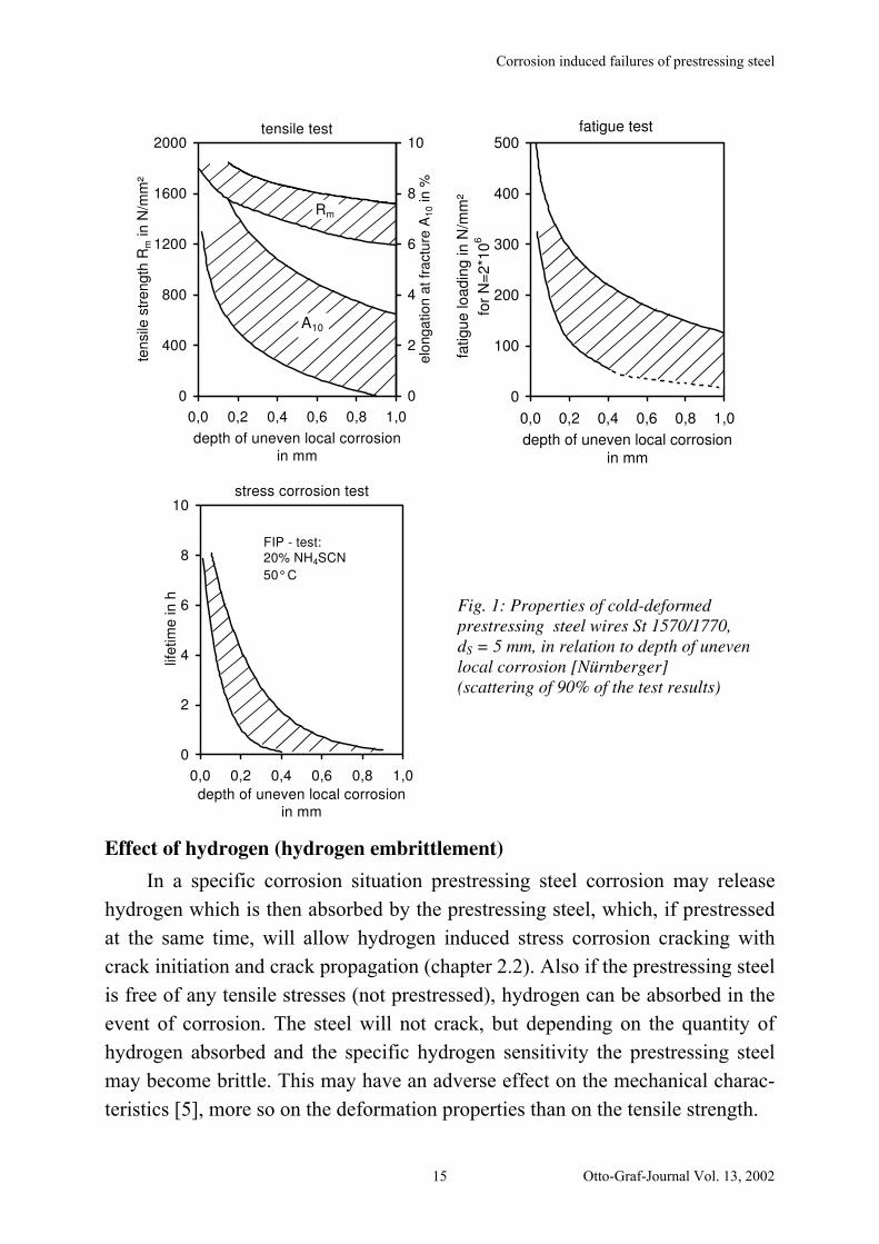
The performance characteristics of corroded prestressing steels can be de-
termined in tensile, fatigue and stress corrosion tests (Fig. 1). Such tests to estab-
lish the residual load bearing capacity will, for instance, be carried out while in-
specting older buildings, after damaged prestressing steel samples had been
drawn. This might help to gain the knowledge for necessary repair.
High strength prestressing steels show a far more sensitive reaction to cor-
rosion attack than reinforcing steels, and this increasingly in the sequence tensile
test - fatigue test – stress corrosion test [4]. In case of uneven local corrosion a
corrosion depth of 0.6 mm may suffice for breaking a cold deformed wire under
tension of 70 % of the specified tendon strength of about 1800 N/mm2 (Fig. 1,
tensile test).
At pitting depth of above 0.2 mm cold drawn wires may show fatigue lim-
its (fatigue limits for stress cycles of N = 2 · 106) of 100 N/mm2 and less (Fig. 1,
fatigue test). Like-new smooth surfaced steels normally show a fatigue limit of
more than 400 N/mm2.
In all the performance characteristics of prestressing steels local corrosion
attack has the most detrimental effect on the behaviour to hydrogen induced cor-
rosion cracking. In a test developed by FIP the prestressing steel is immersed
under tension into an ammonium thiocyanate solution. A minimum and average
time of exposure before failure is specified. For cold drawn wire and strand
these values are in the order of 1.5, respectively 5 hours. In this example these
life times are underrun at corrosion depths of > 0.2 mm (Fig. 1, stress corrosion
test).
14
Corrosion induced failures of prestressing steel
fatigue test
0
100
200
300
400
500
0,0 0,2 0,4 0,6 0,8 1,0
depth of uneven local corrosionin mm
fatig
ue
lo
ad
ing
in
N/m
m²
for
N=
2*1
06
tensile test
0
400
800
1200
1600
2000
0,0 0,2 0,4 0,6 0,8 1,0
depth of uneven local corrosionin mm
tensile
str
ength
Rm
in
N/m
m²
0
2
4
6
8
10
elo
ngation a
t fr
actu
re A
10 in
%
Rm
A10
stress corrosion test
0
2
4
6
8
10
0,0 0,2 0,4 0,6 0,8 1,0
depth of uneven local corrosionin mm
life
tim
e in
h
FIP - test:20% NH4SCN
50° C
Fig. 1: Properties of cold-deformed prestressing steel wires St 1570/1770, dS = 5 mm, in relation to depth of uneven local corrosion [Nürnberger] (scattering of 90% of the test results)
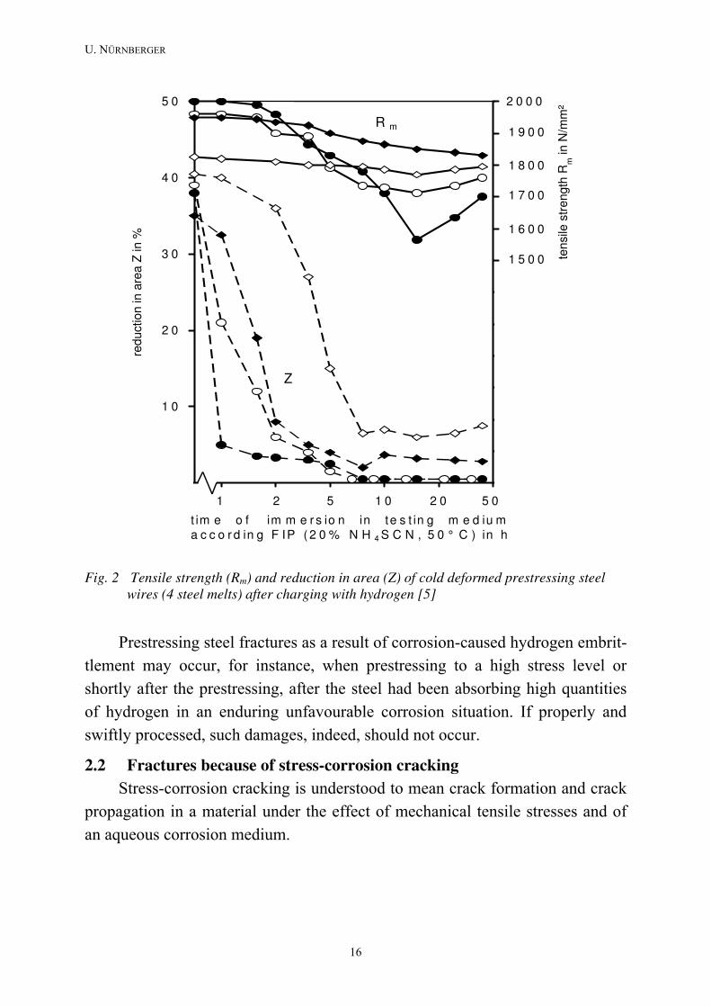
Effect of hydrogen (hydrogen embrittlement)
In a specific corrosion situation prestressing steel corrosion may release
hydrogen which is then absorbed by the prestressing steel, which, if prestressed
at the same time, will allow hydrogen induced stress corrosion cracking with
crack initiation and crack propagation (chapter 2.2). Also if the prestressing steel
is free of any tensile stresses (not prestressed), hydrogen can be absorbed in the
event of corrosion. The steel will not crack, but depending on the quantity of
hydrogen absorbed and the specific hydrogen sensitivity the prestressing steel
may become brittle. This may have an adverse effect on the mechanical charac-
teristics [5], more so on the deformation properties than on the tensile strength.
Otto-Graf-Journal Vol. 13, 2002 15
U. NÜRNBERGER
0
1 0
2 0
3 0
4 0
5 0
0 1 0 2 0 3 0 4 0 5 0 6 0
t im e o f im m e r s io n in te s t in g m e d iu ma c c o r d in g F IP ( 2 0 % N H 4 S C N , 5 0 ° C ) in h
reduction in a
rea Z
in %
- 1 0 0
7 5
2 5 0
4 2 5
6 0 0
7 7 5
9 5 0
1 1 2 5
1 3 0 0
1 4 7 5
1 6 5 0
1 8 2 5
2 0 0 0
tensile
str
ength
Rm
in N
/mm
²
Z
R m
1 5 02 01 05 2
1 9 0 0
1 5 0 0
1 6 0 0
1 7 0 0
1 8 0 0
Fig. 2 Tensile strength (Rm) and reduction in area (Z) of cold deformed prestressing steel wires (4 steel melts) after charging with hydrogen [5]
Prestressing steel fractures as a result of corrosion-caused hydrogen embrit-
tlement may occur, for instance, when prestressing to a high stress level or
shortly after the prestressing, after the steel had been absorbing high quantities
of hydrogen in an enduring unfavourable corrosion situation. If properly and
swiftly processed, such damages, indeed, should not occur.
2.2 Fractures because of stress-corrosion cracking Stress-corrosion cracking is understood to mean crack formation and crack
propagation in a material under the effect of mechanical tensile stresses and of
an aqueous corrosion medium.
16
Corrosion induced failures of prestressing steel
Anodic stress-corrosion cracking
In the presence of nitrate-containing non-alkaline electrolytes (pH-value
< 9) unalloyed and low-alloy steels may suffer an anodic stress-corrosion crack-
ing. Crack formation and crack propagation are due to a selective metal dissolu-
tion (e. g. along grain boundaries of the steel structure) with a simultaneous ef-
fect of high mechanical tensile stresses [6] on condition that there is special ten-
dency of the steels to passivate in nitrate-containing aqueous solutions.
In the prestressed concrete construction the media-related pre-conditions,
e.g. in the fertilizer storage and in stable ceilings, can be assumed as a fact. In
stables brickwork, salpetre Ca (NO3)2 may be formed by urea. In the presence of
moisture the nitrates may diffuse into the concrete and may cause stress-
corrosion cracking in the case of pretensioned concrete components affecting the
tension wires if the concrete cover is carbonated due to an inferior quality of the
concrete [6].
A specific nitrate sensitivity of the steels is always a pre-condition for an
anodic stress-corrosion cracking. Low-carbon concrete steels are very suscepti-
ble to nitrate induced stress-corrosion cracking. The prestressing steels currently
in use, however, are highly resistant to this type of corrosion.
Hydrogen induced stress corrosion cracking [6,7]
Fractures of prestressing steel as a rule can be referred to hydrogen induced
stress corrosion cracking (H-SCC). It may happen during the erection of the
construction or during later use. The following conditions are necessary:
• a sensitive material or state,
• a sufficient tension load,
• at least a slight corrosion attack.
The risk of fractures due to hydrogen induced stress corrosion cracking
therefore results from the joint action of very prestressing steel properties and
environmental parameters. What is needed is the presence of hydrogen which
comes into being under certain corrosion conditions in neutral and particularly
in acid aqueous media through the cathodic partial reaction of the corrosion.
Otto-Graf-Journal Vol. 13, 2002 17
U. NÜRNBERGER
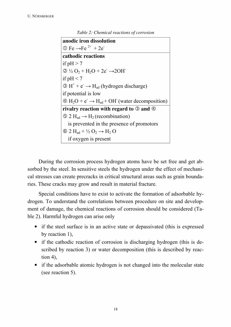
Table 2: Chemical reactions of corrosion
anodic iron dissolution | Fe sFe 2+ + 2e-
cathodic reactions if pH > 7
~ ½ O2 + H2O + 2e- s2OH-
if pH < 7
¡ H+ + e- s Had (hydrogen discharge)
if potential is low
¢ H2O + e- s Had + OH- (water decomposition)
rivalry reaction with regard to ¡ and ¢ £ 2 Had s H2 (recombination)
is prevented in the presence of promotors
⁄ 2 Had + ½ O2 s H2 O
if oxygen is present
During the corrosion process hydrogen atoms have be set free and get ab-
sorbed by the steel. In sensitive steels the hydrogen under the effect of mechani-
cal stresses can create precracks in critical structural areas such as grain bounda-
ries. These cracks may grow and result in material fracture.
Special conditions have to exist to activate the formation of adsorbable hy-
drogen. To understand the correlations between procedure on site and develop-
ment of damage, the chemical reactions of corrosion should be considered (Ta-
ble 2). Harmful hydrogen can arise only
• if the steel surface is in an active state or depassivated (this is expressed
by reaction 1),
• if the cathodic reaction of corrosion is discharging hydrogen (this is de-
scribed by reaction 3) or water decomposition (this is described by reac-
tion 4),
• if the adsorbable atomic hydrogen is not changed into the molecular state
(see reaction 5).
18

Corrosion induced failures of prestressing steel
A reduction of oxygen access may support evolution of adsorbable atomic
hydrogen (then reaction 6 is hindered). Therefore at the surface of corroding
steel the amount of adsorbable hydrogen atoms rises
• with increasing hydrogen concentration (reaction 3 or 4 is accelerated),
• in the presence of so-called promotors (reactions 5 is hindered),
• in an electrolyte impoverished in oxygen (reaction 6 is hindered).
From the practical point of view one can say that hydrogen assisted dam-
ages are only possible
• in acid media or if the steel surface is polarized to low potentials (e. g. if
the prestressing steel has contact with zinc or galvanized steel),
• in the presence of promotors such as sulphides, thiocyanate or compounds
of arsenic or selenium,
• and under crevice conditions, because the electrolyte in the crevice is poor
in oxygen.
Fig. 3: Pitting induced stress corrosion cracking
In concrete structures the attacking medium is mostly alkaline and acid
media are limited to exceptions. Nevertheless, in natural environments the pit-
ting induced H-SCC can take place (Fig. 3). Pitting induced H-SCC means crack
initiation within a corrosion pit. In the corrosion pits the pH-value falls down
because of hydrolysis of the Fe2+-ions. Pitting or spots of local corrosion can be
explained by differential aeration or concentration cells. Especially effective is
Otto-Graf-Journal Vol. 13, 2002 19
U. NÜRNBERGER
the attack of condensation water or salt enriched aqueous solution (bleed water,
chapter 2.1), when erecting the constructions.
In prestressed construction chloride contamination supports a local corro-
sion attack. In the case of sensitive prestressing steel all but minimal contents of
hydrogen can lead to irreversible damages. Then a minimal local corrosion at-
tack without visible corrosion products on the steel surface may lead to steel
fracture.
In prestressed concrete structures all types of uneven local corrosion should
be prevented to exclude failures because of hydrogen assisted cracking.
The preconditions for "classical" stress-corrosion cracking are most readily
to be found in prestressed concrete construction, i. e. crack formation and
propagation under purely static stress. By prestressing the stress amplitudes of
the structure caused e. g. by wind and traffic are kept low. Nevertheless, the oc-
currence of pulsating loads or service-related strain changes of the steels will
raise the crack corrosion risk since it will favour hydrogen induced "non-
classical" stress-corrosion cracking [6]. Plastic flow in steel favours an absorp-
tion of atomic hydrogen.
0
25
50
75
100
125
150
175
200
number of stress reversal
str
ess a
mp
litu
de
2 σ
A in
N/m
m2
agent:
RT without failure
1g/l NH4SCN
105
108
107
1062 864
5 22221111555222111552211 5555
lifetime in hours
2 8642 864
solutionaqueous
withwithout
air
KCll/g5,0
SOKl/g5 42
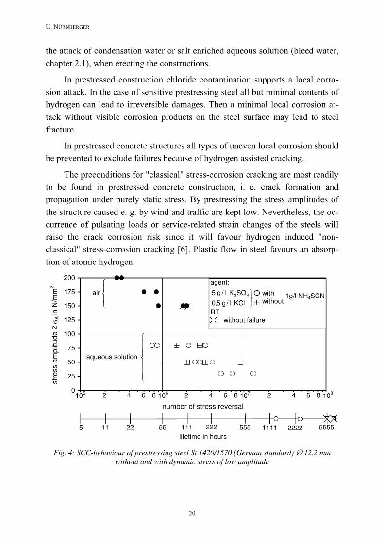
Fig. 4: SCC-behaviour of prestressing steel St 1420/1570 (German standard) ∅ 12.2 mm without and with dynamic stress of low amplitude
20

Corrosion induced failures of prestressing steel
Fig. 4 [8] compares the behaviour of a quenched and tempered prestressing
steel (from a case of damage) sensitive to hydrogen in a stress-corrosion crack-
ing test with and without superimposed fatigue loading of low amplitude (30 –
80 N/mm2). The aqueous test solution contains 5 g/l SO42-,0.5 g/l Cl¯ without
and alternatively with 1 g/l SCN¯ as a promotor for a hydrogen absorption. The
stress-corrosion cracking test under static stress was realized at 80 % of the ten-
sile strength. This stress corresponds to the constant maximum stress in the ten-
sile fatigues test. Fig 4 represents the stress cycle number as a function of the
amplitude, in the course of which also the life time, calculated over the fre-
quency (f = 5s-1), is applied. The stress corrosion test results without superim-
posed fatigue loading are applied at a range of stress of 0 N/mm2. The hydrogen
insensitive steel failed in the "static" test within a test period of 5000 hours in
the promotor-containing solution but did not fail in the promotor-free solution. If
a fatigue test of low amplitude is superimposed, the lifetime in the promotor-
containing solution will more and more decrease with rising amplitude. In the
wave stress it is striking that fractures also occur on steels in the promotor-free
solution.
It was found that in cold deformed prestressing steels the influence of a su-
perimposed fatigue loading on the hydrogen induced stress-corrosion cracking is
revealing itself weaker. These tests lead to the conclusion that already fatigue
loadings of low amplitude or elongations caused by changes in utilization tend
to significantly jeopardize the susceptibility of prestressing steels to stress-
corrosion cracking.
2.3 Fractures because of fatigue and corrosion
Prestressing steels can only be subject to a noticeable steel stress in dy-
namically strained reinforced concrete structures if there is concrete in a cracked
state. The stress amplitudes of prestressing steel due to acting high dynamic
loads ( e. g. a high traffic load of a bridge) may then amount to > 200 N/mm2 in
the crack region. In the uncracked state the steels will show ranges of stress of
clearly less than 100 N/mm2.
Cracks in concrete may occur in partially prestressed structures. Since such
cracks tend to open and to close in a superimposed fatigue stress the following
facts must be considered:
Otto-Graf-Journal Vol. 13, 2002 21

U. NÜRNBERGER
Corrosion fatigue cracking
If corrosion promoting aqueous media penetrate through the concrete crack
to the dynamically stressed tendon, corrosion fatigue cracking is possible al-
though this type of corrosion has not been observed in prestressing steel con-
struction so far. Corrosion fatigue cracking [6] manifests itself in that a metallic
material under dynamic stress in a reactive corrosion medium (water, salt solu-
tion) will show a much more unfavourable fatigue behaviour than under fatigue
loading in air. This can be explained by characteristic interactions of metal
physical and corrosive processes which favour initial precrack formation and
propagation. As opposed to the stress-corrosion cracking the corrosion fatigue
cracking does not require a specifically acting corrosion medium.
In case of post-tensioning tendons the duct made of thin steel sheets does
not offer a lasting corrosion protection and may even suffer fatigue fractures un-
der dynamic stress [9].
A decrease of the fatigue limit by corrosion is the more distinct the higher
the strength of the steel and the more aggressive an attacking medium are.
Hence the high strength prestressing steels, when e. g. simultaneously attacked
by an aqueous chloride-containing medium, may show a very unfavourable fa-
tigue behaviour.
In traffic carrying bridge structures only the low-frequent stresses lead to
high stress amplitudes. This results in additional unfavourable conditions with
regard to corrosion fatigue cracking: with a falling frequency the influence cor-
rosion will increase and the fatigue limit will consequently drop.
For a cold drawn prestressing steel wire Fig. 5 shows a decrease of the cor-
rosion fatigue limit in the sequence air-water-chloride solution. For frequencies
of 0.5s-1 the fatigue limit for stress cycles of 107 is below 100 N/mm2.
The problem of corrosion fatigue cracking of cracked components can be
remedied by sufficient concrete cover and limiting the crack width. This is the
way of keeping pollutants away from the prestressing steel surface.
Fretting corrosion / fretting fatigue
In the vicinity of concrete cracks due to fatigue loading displacements be-
tween the tendon and the injection mortar or the steel duct respectively will oc-
cur in a cracked component. In bended tendons a high radial pressure acts at the
22
Corrosion induced failures of prestressing steel
same time on the fretting prestressing steel surface. If air or oxygen advance to
the fretting location through the concrete crack a fretting corrosion is favoured
[6,10]. Fretting corrosion is described as damaging a metal surface similar to
wear as a result of oscillating friction under radial pressure with a partner. In the
presence of oxygen oxidation of the reactive surface will take place.
In fatigue loaded steels and under fretting corrosion stress at the same time
the fatigue behaviour is under a very unfavourable influence due to fretting fa-
tigue [10]. This is attributable to structural disintegration and the occurrence of
additional tensile strengths in the fretting area. In concrete embedded tendons,
subjected to a relative movement and a radial pressure in the concrete crack be-
tween prestressing steel and duct or injection mortar respectively, tolerable fa-
tigue limits of about 150 N/mm2 for cycles to fracture of 2 x 10⁶ were found
[9,11].
In prestressed concrete constructions also the anchorages of the tendons,
due to fretting corrosion influences, show a fatigue limit which is reduced com-
pared with the free length [12]. Under dynamic stress of the anchored tendon the
fatigue limit, depending on the type of anchorage, is reduced to values between
80 and 150 N/mm2. For this reason, anchorages will always be positioned in ar-
eas of least stress changes. In the fatigue experiment the prestressing steels al-
ways fracture in the force transmitting area, i. e. at the beginning of the anchor-
age. Here, the fatigue limit is reduced due to the presence of shifting between
the prestressing steel and the anchor body and the high radial pressures at the
same time.
In prestressed concrete bridges, however, particularly the coupling joints
proved to be problematic. If such joints crack as a result of imposed stresses
(e.g. due to non uniform sun heating and low amount of reinforcement which
crosses the coupling joint) the tendon couplings will suffer major stress fatigue
cycles from the traffic load which also led to prestressing steel fractures owing
to the stress-sensitive couplings [2,11].
Otto-Graf-Journal Vol. 13, 2002 23

U. NÜRNBERGER
Fig. 5: Fatigue behaviour under pulsating tensile stresses of cold drawn prestressing steel wires (Rm ≈ 1750 N/mm2) in air and corrosion- promoting aqueous solutions (Nürn-berger)
3. CONCLUSION
Depending on the prevailing corrosion situation and the load conditions as
well as the prestressing steel properties the following possibilities of fracturing
must be distinguished:
• Brittle fracture due to exceeding the residual load capacity. Brittle fracture
is particularly promoted by local corrosion attack and hydrogen embrit-
tlement.
• Fracture as a result of hydrogen induced stress-corrosion cracking.
• Fracture as a result of fatigue and corrosion influences, distinguishing be-
tween corrosion fatigue cracking and fretting corrosion/fretting fatigue.
REFERENCES
[1] Durability of post-tensioning tendons. Proceedings of workshop held in
Gent University on 15 - 16 November 2001. fib technical report, bulletin
15
[2] Nürnberger, U.: Analyse und Auswertung von Schadensfällen bei Spann-
stählen. Forschung, Straßenbau und Straßenverkehrstechnik 308 (1980) 1 –
195
24
Corrosion induced failures of prestressing steel
[3] Nürnberger, U.: Influence of material and processing on stress corrosion
cracking of prestressing steel (case studies). Publ. of fib commission 9.5, to
be published
[4] Neubert B., Nürnberger, U.: Erkennen von Spannverfahrensschädigung –
Untersuchung der statischen und dynamischen Kenngrößen in Abhängig-
keit von Rostgrad. Bericht II.6-13675 der FMPA Baden-Württemberg, Ot-
to-Graf-Institut, Stuttgart 31.01.1983
[5] Nürnberger, U., Beul, W.: Entwicklung einfacher und reproduzierbarer
Prüfverfahren für die Empfindlichkeit von Spannstählen gegenüber Span-
nungsrisskorrosion. Bericht 34-14071 der FMPA Baden-Württemberg, Ot-
to-Graf-Institut, Stuttgart 01.03.1996
[6] Nürnberger, U.: Korrosion und Korrosionsschutz im Bauwesen. Bauverlag,
Wiesbaden 1995
[7] Grimme, D., Isecke, B., Nürnberger, U., Riecke, E. M., Uhlig, G.: Span-
nungsrisskorrosion in Spannbetonbauwerken. Verlag Stahleisen mbH, Düs-
seldorf 1983
[8] Nürnberger, U., Beul, W.: Wasserstoffinduzierte Spannungsrisskorrosion
von zugschwellbeanspruchten Spannstählen, S. 302 – 309; in "Bewehrte
Betonbauteile unter Betriebsbedingungen". Wiley-VCH Verlag
[9] Cordes, H.: Dauerhaftigkeit von Spanngliedern unter zyklischen Beanspru-
chungen. Sachstandsbericht. Schriftenreihe Deutscher Ausschuß für Stahl-
beton 370 (1986)
[10] Patzak, M.: Die Bedeutung der Reibkorrosion für nichtruhende Veranke-
rungen und Verbindungen metallischer Bauteile des konstruktiven Ingeni-
eurbaus. Dissertation Universität Stuttgart, 1979
[11] König, G., Maurer, R., Zichner, T.: Spannbeton-Bewährung im Brücken-
bau. Springer Verlag Berlin-Heidelberg-New York-London-Paris-Tokyo,
1986
[12] Rehm, G., Nürnberger, U., Patzak, M.: Keil- und Klemmverankerungen für
dynamisch beanspruchte Zugglieder aus hochfesten Stählen. Bauingenieur
52 (1977) 287 – 298
Otto-Graf-Journal Vol. 13, 2002 25

U. NÜRNBERGER
26
Load bearing behaviour of fastenings with concrete screws
LOAD BEARING BEHAVIOUR OF FASTENINGS WITH CONCRETE SCREWS
TRAGVERHALTEN VON BEFESTIGUNGEN MIT SCHRAUBDÜBELN
COMPORTEMENT SOUS CHARGE DES ANCRAGES AVEC VIS D'ANCRAGE
Jürgen H. R. Küenzlen and Rolf Eligehausen
SUMMARY
Concrete screws are a relatively new fastening system. Their main
advantage compared to traditional post-installed fastening systems is a quick and
easy installation. A hole is drilled into the concrete and threads are cut in the
concrete by the screw as it is installed.
Concrete screws transfer tensile loads into the base material by mechanical
interlock of the threads. Due to their load-bearing mechanism, concrete screws
with a technical approval of the DIBt can be used for fastenings in cracked and
non-cracked concrete.
The typical failure mechanism for concrete screws is concrete-cone failure.
With increasing embedment depth the ratio of the depth of the concrete failure
cone to the embedment depth decreases. The failure load of concrete screws
with continuous threads along the entire embedment depth increases
proportionally to hef1,5 (hef = effective embedment depth), but it is about 20 %
smaller than the failure load of expansion and undercut anchors with the same
embedment depth.
In order for concrete screws to function properly, the threads cut into the
wall of the drilled hole must not be damaged during the installation. This
requirement is achieved by using the embedment depth defined in the Technical
Approvals.
Otto-Graf-Journal Vol. 13, 2002 27

J. H. R. KÜENZLEN, R. ELIGEHAUSEN
ZUSAMMENFASSUNG
Schraubdübel sind ein relativ neues Befestigungssystem. Ihr großer Vorteil
liegt in der einfachen und schnellen Montage. Es wird ein Loch in den Beton
gebohrt, in das der Schraubdübel beim Setzen ein Gewinde schneidet.
Schraubdübel werden in Durchsteckmontage gesetzt.
Schraubdübel übertragen eine angreifende Zuglast über mechanische
Verzahnung der Gewindeflanken, die in die Bohrlochwand einschneiden, in den
Untergrund. Aufgrund ihres Tragmechanismus sind bauaufsichtlich zugelassene
Schraubdübel für Befestigungen im ungerissenen und gerissenen Beton
geeignet.
Das Versagen erfolgt durch Betonausbruch, wobei mit zunehmender
Verankerungstiefe das Verhältnis von Tiefe des Ausbruchkegels zu
Verankerungstiefe abnimmt. Die Bruchlast steigt bei Schraubdübeln mit einem
über die gesamte Verankerungstiefe durchgehende Gewinde proportional zu
hef1,5 an (hef = Verankerungstiefe), jedoch ist sie unter sonst gleichen
Verhältnissen ca. 20 % niedriger als die Betonausbruchlast von Spreiz- und
Hinterschnittdübeln.
Damit Schraubdübel ordnungsgemäß funktionieren, dürfen die in den
Beton geschnittenen Gewindegänge nicht während der Montage beschädigt
werden. Diese Bedingung wird bei Einhaltung der in den bauaufsichtlichen
Zulassungen festgelegten Verankerungstiefe eingehalten.
RESUME
Les vis d'ancrage sont un système de ancrage relativement nouveau. Leur
principal avantage est une installation rapide et facile. Un trou est foré dans le
béton et les spires sont taraudées dans le béton par la vis lors de sa mise en
place. Les vis d'ancrage transfèrent les charges de tension dans le béton par le
couplage mécanique des spires. En raison de leur mécanisme porteur, les vis
d'ancrage avec un agrément technique du DIBt peuvent être utilisées pour des
ancrages dans le béton fissuré et non-fissuré. Le mécanisme de rupture pour les
vis d'ancrage est la rupture par cône de béton. Une augmentation de la
profondeur d'encrage est accompagnée d'une diminution du rapport de la
profondeur du cône de béton à la profondeur d'encrage. La charge de rupture des
vis d'ancrage à filetage continu sur toute la profondeur d'ancrage augmente
proportionnellement à hef1,5 (hef = profondeur d'ancrage effective), elle est
28
Load bearing behaviour of fastenings with concrete screws
néanmoins environ 20 % inférieure à la charge de rupture des chevilles à
expansion et des chevilles à verrouillage de forme avec la même profondeur
d'ancrage. Afin que les vis d'ancrage puissent fonctionner correctement, les
filetages taraudés dans le béton ne doivent pas être endommagés pendant
l'installation. Ceci est réalisé si l'on respecte la profondeur d'ancrage définie
dans l'agrément technique.
KEYWORDS: concrete screw, shearing-off of threads, mechanical interlock
1. INTRODUCTION
Concrete screws are a relatively new fastening system. Their main
advantage compared to traditional post-installed fastening systems is a quick and
easy installation. A hole is drilled into the concrete and threads are cut in the
concrete by the screw as it is installed.
In Germany there are currently three different types of concrete screws
from three manufacturers approved by the DIBt for fastenings with single
anchors and groups in cracked and non-cracked concrete [1,2,3]. Further
technical approvals exist for suspended ceilings and other comparable static
systems.
During the technical approval process a large number of tests were
conducted at the Institute of Construction Materials at the University of
Stuttgart. Furthermore, the load bearing behaviour of concrete screws was
systematically investigated through experimental and numerical studies within
the scope of a research project. Important results of research reports [5, 6, 7, 8]
are presented below.
2. CONCRETE SCREWS WITH TECHNICAL APPROVAL OF THE DIBT
Figure 1 shows three concrete screws with a technical approval by the
DIBt. The screws are intended for a drill hole diameter of d0 = 10mm and are
made of galvanised steel. They differ principally in steel strength, core diameter
and thread geometry. Two of the concrete screws have small steel teeth at the
end of the screw for cutting the threads into the concrete. The third concrete
screw has alternating high and low screw threads. Grooves are cut into the
concrete by the specially formed high screw threads.
Otto-Graf-Journal Vol. 13, 2002 29

J. H. R. KÜENZLEN, R. ELIGEHAUSEN
Figure 1: Concrete screws (d0 = 10mm) with a technical approval of the DIBt
Concrete screws made of galvanised steel intended for a drill hole diameter
of d0 = 5mm and d0 = 6mm are approved for suspended ceilings. Concrete
screws with a drill bit diameter of d0 = 8mm and d0 =10mm have a technical
approval for the fastenings of statically determined and undetermined supported
components in cracked and non-cracked concrete. Fastenings with single
anchors and groups are allowed.
Technical approvals also exist for concrete screws made of stainless steel
with drill bit diameters of d0 = 6mm to d0 = 10mm. To aid in the cutting of
threads into the concrete, one concrete screw has an end made of galvanised
steel. This end cannot be added to the embedment depth. Another concrete
screw has small cutting pins made of carbon steel in the first turns to cut the
threads into the concrete.
While concrete screws made of galvanised steel are only allowed for use in
dry environments, the concrete screws made of stainless steel can be used
outdoors, in industrial environments and near the sea.
Concrete screws made of galvanised steel are cold-rolled and subsequently
tempered and heat-treated. Residual stress and incipient cracks in the steel can
result from this process. To insure flawless products, special tests must be
carried out during manufacturing within the scope of the internal quality control.
Concrete screws made of galvanised steel, which are produced according to
requirements for the technical approvals, have an indefinite lifespan in dry
environments. If concrete screws made of galvanised steel are used in
environments with a high corrosion risk (e.g. outdoors), a brittle failure can
occur as a consequence of stress corrosion cracking. The time until failure
cannot be predicted. In these cases concrete screws made of stainless steel (or
other types of fastenings) must be used.
30
Load bearing behaviour of fastenings with concrete screws
In the following section results of tests with the concrete screws type 1 to
type 3 are presented. It is pointed out that the numbering of the concrete screw
types is not the same as shown in Figure 1 or in the cited references.
3. LOAD BEARING BEHAVIOUR OF CONCRETE SCREWS
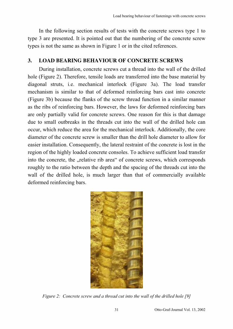
During installation, concrete screws cut a thread into the wall of the drilled
hole (Figure 2). Therefore, tensile loads are transferred into the base material by
diagonal struts, i.e. mechanical interlock (Figure 3a). The load transfer
mechanism is similar to that of deformed reinforcing bars cast into concrete
(Figure 3b) because the flanks of the screw thread function in a similar manner
as the ribs of reinforcing bars. However, the laws for deformed reinforcing bars
are only partially valid for concrete screws. One reason for this is that damage
due to small outbreaks in the threads cut into the wall of the drilled hole can
occur, which reduce the area for the mechanical interlock. Additionally, the core
diameter of the concrete screw is smaller than the drill hole diameter to allow for
easier installation. Consequently, the lateral restraint of the concrete is lost in the
region of the highly loaded concrete consoles. To achieve sufficient load transfer
into the concrete, the „relative rib area“ of concrete screws, which corresponds
roughly to the ratio between the depth and the spacing of the threads cut into the
wall of the drilled hole, is much larger than that of commercially available
deformed reinforcing bars.
Figure 2: Concrete screw and a thread cut into the wall of the drilled hole [9]
Otto-Graf-Journal Vol. 13, 2002 31

J. H. R. KÜENZLEN, R. ELIGEHAUSEN
a)
b)
Figure 3: Transmission of tension load into concrete
a) Concrete screw
b) Cast-in-place deformed reinforcing bar
4. INSTALLATION OF CONCRETE SCREWS
Concrete screws are normally screwed into the concrete using an electric-
screw-gun. In technical approvals the power class [2,3] or the type of electric-
screw-gun [1] is specified. The threads cut into the concrete must not be
destroyed during installation. Limiting the applied torque can do this. Concrete
screws can also be screwed in with a torque wrench. It cannot be excluded that
concrete screws should not be screwed in using a commercial screw-wrench,
because the torque necessary for tightening up after the screw head reaches the
attachment can range between wide limits and therefore the threads cut into the
concrete might be destroyed.
The necessary installation torque for cutting the threads into the concrete
should be small in order to achieve an easy installation. Moreover, the resistance
against shearing-off of the threads should be as high as possible, so that the
threads cut into the concrete are not destroyed while tightening up the concrete
screws.
Figure 4 shows the measured torques while screwing in a concrete screw
(drill bit diameter d0 = 8mm) dependent on the swing angle. The failure
happened by shearing-off of the threads. The anchorage material consisted of
fine-grained concrete (maximum aggregate size 8mm) of the strength class B25.
32

Load bearing behaviour of fastenings with concrete screws
0 250 500 750 1000 1250 1500 1750 2000
Drehwinkel [Grad]
0
25
50
75
100
125
Dre
hm
om
en
t [N
m]
Figure 4: Typical relationship between torque moment and swing angle (Concrete B25,
grading curve BC 8, d0= 8mm, Failure mode: Shearing-off of the thread [10]
Before the screw head reached the attachment, the necessary installation
torque varied only slightly. If the concrete contains coarser aggregates, torque
peaks can occur if a thread is cut into a big piece of aggregate.
After the screw head reaches the attachment, the torque on the concrete
screw rises sharply to the peak value TD. Subsequently, the shearing-off of the
threads begins and the torque decreases rapidly to zero. The damage to the
concrete threads after overtightening the concrete screw is shown in Figure 5.
Figure 5a shows the threads after the screw head reaches the attachment
(installation torque TE). For comparison, the threads cut into the concrete by the
concrete screw (d0 = 10mm) at the remaining torques of TRest ~ 0,75TD,m and
TRest ~ 0,19TD,m after reaching the peak value TD,m are shown in Figure 5b and
Figure 5c, respectively.
a) b) c)
Figure 5: Threads cut into the wall of the drilled hole, concrete screw type 2 [10]
a) Tinst = TE
b) TRest = 100Nm (~0,75 TD,m)
c) TRest = 25Nm (~0,19 TD,m)
Otto-Graf-Journal Vol. 13, 2002 33
J. H. R. KÜENZLEN, R. ELIGEHAUSEN
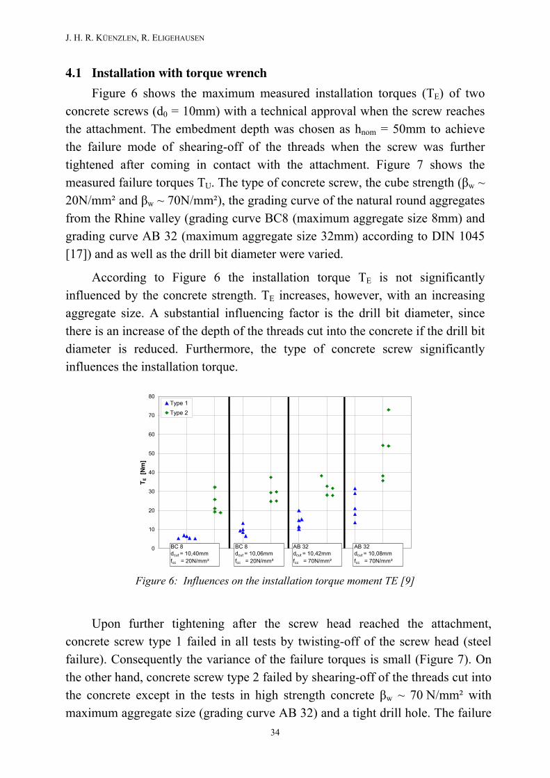
4.1 Installation with torque wrench
Figure 6 shows the maximum measured installation torques (TE) of two
concrete screws (d0 = 10mm) with a technical approval when the screw reaches
the attachment. The embedment depth was chosen as hnom = 50mm to achieve
the failure mode of shearing-off of the threads when the screw was further
tightened after coming in contact with the attachment. Figure 7 shows the
measured failure torques TU. The type of concrete screw, the cube strength (くw ~
20N/mm² and くw ~ 70N/mm²), the grading curve of the natural round aggregates
from the Rhine valley (grading curve BC8 (maximum aggregate size 8mm) and
grading curve AB 32 (maximum aggregate size 32mm) according to DIN 1045
[17]) and as well as the drill bit diameter were varied.
According to Figure 6 the installation torque TE is not significantly
influenced by the concrete strength. TE increases, however, with an increasing
aggregate size. A substantial influencing factor is the drill bit diameter, since
there is an increase of the depth of the threads cut into the concrete if the drill bit
diameter is reduced. Furthermore, the type of concrete screw significantly
influences the installation torque.
0
10
20
30
40
50
60
70
80
TE [N
m]
Type 1
Type 2
BC 8
dcut = 10,40mm
fcc = 20N/mm²
BC 8
dcut = 10,06mm
fcc = 20N/mm²
AB 32
dcut = 10,42mm
fcc = 70N/mm²
AB 32
dcut = 10,08mm
fcc = 70N/mm²
Figure 6: Influences on the installation torque moment TE [9]
Upon further tightening after the screw head reached the attachment,
concrete screw type 1 failed in all tests by twisting-off of the screw head (steel
failure). Consequently the variance of the failure torques is small (Figure 7). On
the other hand, concrete screw type 2 failed by shearing-off of the threads cut into
the concrete except in the tests in high strength concrete くw ~ 70 N/mm² with
maximum aggregate size (grading curve AB 32) and a tight drill hole. The failure
34

Load bearing behaviour of fastenings with concrete screws
torques in case of shearing-off of the threads are barely affected by the concrete
strength and the composition of the concrete. However, they increase as was the
case for the installation torques, with decrease of the drill bit diameter.
The different failure modes of concrete screw type 1 and type 2 can mainly
be attributed to the fact that the steel strength of concrete screw type 2 is higher
than the steel strength of type 1. For that reason concrete screw type 2 needs a
larger embedment depth than type 1 to reach the failure mode of steel failure.
0
50
100
150
200
250
TU [N
m]
steel failure, Type 1 steel failure, Type 2shearing off of thread, Type 2
BC 8
dcut = 10,40mm
fcc = 20N/mm²
BC 8
dcut = 10,06mm
fcc = 20N/mm²
AB 32
dcut = 10,42mm
fcc = 70N/mm²
AB 32
dcut = 10,08mm
fcc = 70N/mm²
Figure 7: Influences on the failure torque moment TU [9]
By increasing the embedment depth the installation torque increases only
slightly because the threads are mainly cut into the concrete by the flanks of the
screw thread at the head of the screw.
On the other hand, the failure torque in the case of shearing-off of the
threads cut in the concrete increases with increasing embedment depth (Figure
8), because more threads have to be sheared off. The embedment depth required
by the technical approvals with hnom œ 70mm is significantly larger than the
embedment depth used in the tests shown in Figure 7. This ensures that the
failure mode steel failure occurs and not the failure mode shearing-off of the
threads (Figure 8) if the concrete screw is overtightened during installation.
Otto-Graf-Journal Vol. 13, 2002 35

J. H. R. KÜENZLEN, R. ELIGEHAUSEN
0
50
100
150
200
250
300
0 10 20 30 40 50 60 70 80
hnom [mm]
Failu
re M
om
en
t [N
m]
steel failure
concrete failure
setting depth according to Technical Approval
fcc ˜ 30N/mm²
grading curve BC 8
Figure 8: Influence of the embedment depth on the failure torque moments [11]
4.2 Installation with electric-screw-gun
While the installation of a concrete screw with a torque wrench or a screw-
wrench requires more than 30 seconds for the screw head to reach the
attachment, installation with a high-performance electric-screw-gun requires
only one to two seconds. For this reason, in practice concrete screws are usually
screwed-in with an electric-screw-gun. In the setting tests electric-screw-guns
with a maximum moment higher than the steel failure torque moment of the
concrete screws were used. Nevertheless, the concrete screws failed by shearing-
off of the threads after the screw head reached the attachment. The time between
reaching the attachment and shearing-off of the threads tK increases with
increasing embedment depth (Figure 9).
0
3
6
9
12
15
40 45 50 55 60 65 70 75
hnom [-]
t K [
sec]
test stopped
Figure 9: Influence of the embedment depth on the time until shearing-off of the threads cut
into the wall of the drilled hole (d0 = 10mm, grading curve BC 8, くw = 26N/mm², dcut =
10,41mm, electric-screw-gun 1)
36
Load bearing behaviour of fastenings with concrete screws
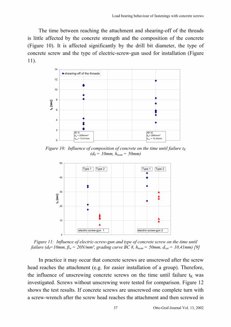
The time between reaching the attachment and shearing-off of the threads
is little affected by the concrete strength and the composition of the concrete
(Figure 10). It is affected significantly by the drill bit diameter, the type of
concrete screw and the type of electric-screw-gun used for installation (Figure
11).
0
2
4
6
8
10
12
14
t K [
sec]
shearing-off of the threads
BC 8
くw = 20N/mm²
dcut = 10,41mm
AB 32
くw= 26N/mm²
dcut = 10,43mm
Figure 10: Influence of composition of concrete on the time until failure tK
(d0 = 10mm, hnom = 50mm)
0
10
20
30
40
50
tK [
se
c]
electric-screw-gun 1 electric-screw-gun 2
Type 1 Type 2 Type 1 Type 2
Figure 11: Influence of electric-screw-gun and type of concrete screw on the time until
failure (d0=10mm, くw = 20N/mm², grading curve BC 8, hnom = 50mm, dcut = 10,41mm) [9]
In practice it may occur that concrete screws are unscrewed after the screw
head reaches the attachment (e.g. for easier installation of a group). Therefore,
the influence of unscrewing concrete screws on the time until failure tK was
investigated. Screws without unscrewing were tested for comparison. Figure 12
shows the test results. If concrete screws are unscrewed one complete turn with
a screw-wrench after the screw head reaches the attachment and then screwed in
Otto-Graf-Journal Vol. 13, 2002 37

J. H. R. KÜENZLEN, R. ELIGEHAUSEN
again with an electric-screw-gun, the minimum time until failure tK decreases in
comparison with concrete screws that were not unscrewed. If the unscrewing of
the concrete screw takes place with an electric-screw-gun, the time until failure
tK decreases significantly because it is not possible to unscrew concrete screws
in a controlled manner with an electric-screw-gun.
0
4
8
12
16
tK [
sec]
installation with
electric-screw-gun
installation /unscrewing /
installation with electric-
screw-gun
installation with electric-screw-
gun, unscrewing with torque
wrench, installation with electric-
screw-gun
Figure 12: Influence of unscrewing of concrete screws on the time tK until failure (d0 = 10mm,
fcc = 26N/mm², grading curve BC8, dcut = 10,44mm, hnom = 60mm, electric-screw-gun 1)
4.3 Remaining load-carrying capacity
To investigate the influence of the installation torque, i. e. the over-
tightening of the concrete screw, on the pull-out failure load, the concrete screws
were installed until the screw head reached the attachment (T = TE), prestressed
with T ~ 0,9 TD,m or until the torque moment fell to a preset value T = TRest after
reaching the maximum torque. Afterwards the concrete screws were pulled out.
Figure 13 shows the measured failure loads depending on the installation torque.
If the torque of the concrete screw is stopped immediately after reaching the
maximum torque, the measured pull-out failure loads are in the same range like
in the tests with concrete screws that were prestressed with T = TE or with
T ~ 0,9 TD,m. Furthermore, the load-displacement behaviour does not differ
significantly (Figure 14). If the concrete screws are turned further, the failure
load falls rapidly, because the threads cutting into the wall of the drilled hole are
destroyed (cp. Figure 5). Furthermore, the load-displacement behaviour is less
favourable. The behaviour shown in Figure 13 and Figure 14 also applies to
other types of concrete screws if they are seated with an embedment depth at
which shearing-off of the threads is possible.
38

Load bearing behaviour of fastenings with concrete screws
0
2
4
6
8
10
12
14
16
00,20,40,60,811,21,4
T/TU,m [-]
Nu [
kN
]
T = TE
before shearing
0,9
TU,m = 135Nm
after reaching TU,m
Figure 13: Influence of torque before and after reaching the failure torque on the pull-out
load (d0 = 10mm, hnom = 50mm, dcut = 10,42 mm, fcc = 30N/mm²)
0 2 4 6 8 10
s [mm]
0
2
4
6
8
10
12
14
16
Nu
[kN
]
T = 0.19xTD,m
T = 0,75xTD,m
T = TE
T = 0,19 TD,m
T = 0,75 TD,m
Figure 14: Influence of the torque moment before and after reaching the
failure torque on the load-displacement curves
4.4 Required embedment depth
In practice it cannot be excluded that concrete screws are further tightened
after the screw head reaches the attachment, e. g. if the electric-screw-gun is not
stopped immediately or if the attachment should be tightened against the surface
of the concrete slab with a standard screw-wrench. Unscrewing of the concrete
screws and screwing them in again can also occur. This may damage the threads
cut into the wall of the drilled hole, if the embedment depth is not deep enough
because in practice it is normally not possible to stop the installation after
reaching the maximum torque TD. This has been shown by experiences in
practice. A check of concrete screws (d0 = 6mm) that were seated with a small
embedment depth showed that shearing-off of the threads during the installation
had occurred with about 15% of the screws.
Otto-Graf-Journal Vol. 13, 2002 39
J. H. R. KÜENZLEN, R. ELIGEHAUSEN
To avoid damage of the threads cut into the concrete, the embedment depth
of the concrete screws with a technical approval of the DIBt was defined such
that steel failure and not shearing-off of the threads will occur during installation
with a standard screw wrench (Figure 8). At this embedment depth a long period
of time is needed to shear-off of the threads using an electric-screw-gun. It is
assumed that in practice a time period as long as this is not applied.
Concrete screws with a larger core diameter than the concrete screws with
a technical approval have very high torque moments in the case of steel failure.
Therefore, it makes no sense to evaluate the minimum embedment depth of
these concrete screws since that steel failure occurs. Presently a new concept for
concrete screws with d0 > 10mm is being developed to avoid the damage of the
threads cut into the concrete during the installation.
5. LOAD BEARING BEHAVIOUR OF CONCRETE SCREWS
5.1 Load-displacement behaviour and failure mode
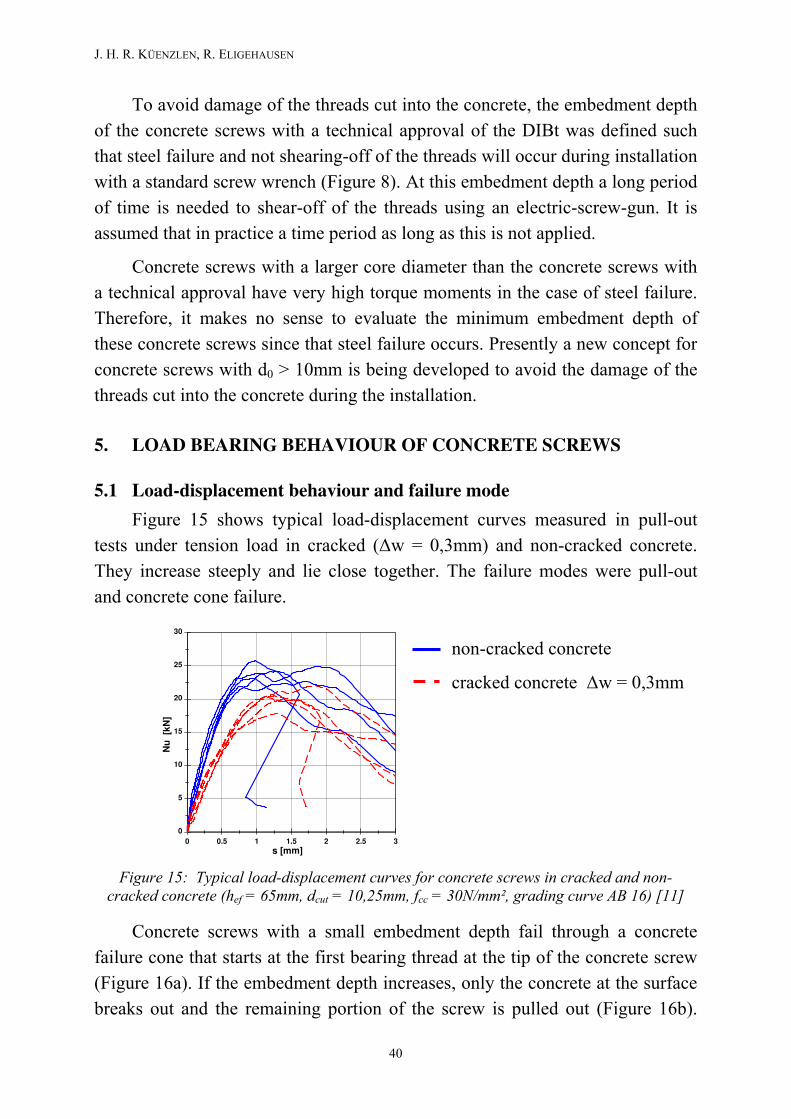
Figure 15 shows typical load-displacement curves measured in pull-out
tests under tension load in cracked (〉w = 0,3mm) and non-cracked concrete.
They increase steeply and lie close together. The failure modes were pull-out
and concrete cone failure.
0 0.5 1 1.5 2 2.5 3
s [mm]
0
5
10
15
20
25
30
Nu
[k
N]
non-cracked concrete
cracked concrete 〉w = 0,3mm
Figure 15: Typical load-displacement curves for concrete screws in cracked and non-
cracked concrete (hef = 65mm, dcut = 10,25mm, fcc = 30N/mm², grading curve AB 16) [11]
Concrete screws with a small embedment depth fail through a concrete
failure cone that starts at the first bearing thread at the tip of the concrete screw
(Figure 16a). If the embedment depth increases, only the concrete at the surface
breaks out and the remaining portion of the screw is pulled out (Figure 16b).
40

Load bearing behaviour of fastenings with concrete screws
The observed failure modes differ from the failure mode of expansion anchors
and undercut anchors. These anchors transfer the load into the concrete near the
end of the embedment depth and the concrete cone failure begins near the end of
the anchor. On the other hand, concrete screws discharge the load over the entire
embedment depth into the concrete.
The failure mode shown in Figure 16 is similar to that of bonded anchors
but the failure load of bonded anchors increases nearly linearly with increasing
embedment depth (hef) [12]. Whereas the failure load of concrete screws
increases by hef1,5 (see section 5.2.1). Therefore, the failure of concrete screws is
due to exceedence of the concrete tension strength in the failure cone and not to
pullout as for bonded anchors.
a)
b)
Figure 16: Typical concrete failure cones [9]
a) hnom = 50mm
b) hnom = 90mm
5.2 Failure Loads
To clarify the influence of different parameters on the failure loads of
concrete screws, pull-out tests in concrete slabs with a cube strength of about くw
~ 30N/mm² were performed. The concrete slabs were produced from concrete
with a grading curve AB16 (aggregates with maximum size 16mm) according to
DIN 1045 [17]. Natural round aggregates from the Rhine valley were used. For
drilling of the holes, drill bits with medium bit diameter according to [4] were
used. The measured failure loads were normalized by くw0,5 to くw = 30N/mm²
because the failure is caused by exceedence of the concrete tension strength.
Otto-Graf-Journal Vol. 13, 2002 41

J. H. R. KÜENZLEN, R. ELIGEHAUSEN
Influence of the embedment depth
Figure 17 shows the measured failure loads of concrete screws produced by
manufacturer 1 for various embedment depths hef. The investigated parameter is
the drill hole diameter d0. The effective embedment depth was determined
according to equation (1).
hef = hnom – 0,5*h – hS (1)
with:
hnom = length between end of concrete screw and concrete surface
h = threaded length of concrete screw
hS = length of screw without thread
Equation (1) considers that load discharge starts with a transfer from the
top of the concrete screw that is dependent on the kind of thread of the concrete
screw. It enables a better comparison of the test results of concrete screws from
different manufacturers, i. e. with different kind of threads.
According to Figure 17 the failure loads of concrete screws increase
proportionally to hef1,5. That relation also applies to expansion and undercut
anchors failing by concrete cone failure. Figure 17 applies to concrete screws
with threads over the complete embedment depth. If concrete screws only have
threads over part of the embedment depth, the failure load will not increase after
reaching a certain embedment depth, because the failure mode changes to pull-
out failure (shearing-off of the concrete between the screw flanks). This is
similar to the behaviour of torque-controlled expansion anchors, where the
failure mode changes with increasing embedment depth from concrete cone
failure to pull-through failure [14].
0
10
20
30
40
50
60
70
0 20 40 60 80 100 120
hef [mm]
Nu [
kN
]
do = 8mm
do = 10mm
do = 12mm
do = 14mm
do = 18mm
Nu = g*hef1,5
くw = 30N/mm²
Nu = Nu,Versuch*(30/くw)0,5
Figure 17: Influence of embedment depth on failure load
42
Load bearing behaviour of fastenings with concrete screws
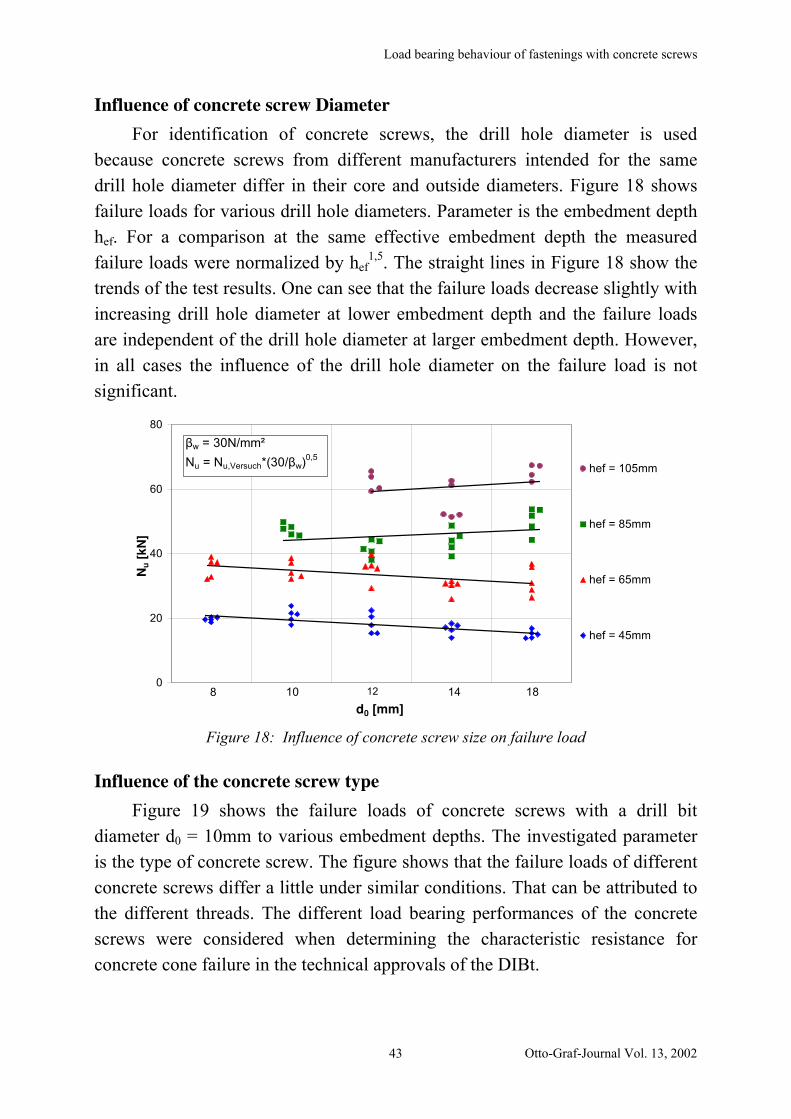
Influence of concrete screw Diameter
For identification of concrete screws, the drill hole diameter is used
because concrete screws from different manufacturers intended for the same
drill hole diameter differ in their core and outside diameters. Figure 18 shows
failure loads for various drill hole diameters. Parameter is the embedment depth
hef. For a comparison at the same effective embedment depth the measured
failure loads were normalized by hef1,5. The straight lines in Figure 18 show the
trends of the test results. One can see that the failure loads decrease slightly with
increasing drill hole diameter at lower embedment depth and the failure loads
are independent of the drill hole diameter at larger embedment depth. However,
in all cases the influence of the drill hole diameter on the failure load is not
significant.
0
20
40
60
80
Nu [
kN
]
hef = 105mm
hef = 85mm
hef = 65mm
hef = 45mm
8 1210 1814
d0 [mm]
くw = 30N/mm²
Nu = Nu,Versuch*(30/くw)0,5
Figure 18: Influence of concrete screw size on failure load
Influence of the concrete screw type
Figure 19 shows the failure loads of concrete screws with a drill bit
diameter d0 = 10mm to various embedment depths. The investigated parameter
is the type of concrete screw. The figure shows that the failure loads of different
concrete screws differ a little under similar conditions. That can be attributed to
the different threads. The different load bearing performances of the concrete
screws were considered when determining the characteristic resistance for
concrete cone failure in the technical approvals of the DIBt.
Otto-Graf-Journal Vol. 13, 2002 43

J. H. R. KÜENZLEN, R. ELIGEHAUSEN
0
10
20
30
40
50
60
0 10 20 30 40 50 60 70 80 90
hef [mm]
Nu [
kN
]
Typ 1
Typ 2
くw = 30N/mm²
Nu = Nu,Versuch*(30/くw)0,5
Nu = g*hef1,5
Figure 19: Influence of the type of concrete screw (d0 = 10mm) on the failure loads
Influence of Screw Spacing
To investigate the influence of the screw spacing on the failure loads, groups
with four concrete screws in concrete with the concrete strength near くw ~
30N/mm² were tested. The screw spacing was varied. At small spacing the
groups failed by a combined concrete cone failure (Figure 20a). At a spacing of
s = 2 hnom a changeover to several failure cones was observed (Figure 20b).
a)
b)
Figure 20: Concrete failure cone of square groups with concrete screws
a) s = 1 hnom and
b) s = 2 hnom (d0 = 10mm, hnom = 70mm)
While the screw spacing does not significantly influence the stiffness at the
beginning of the tests, the failure loads and the displacement at failure load
increase with increasing screw spacing (Figure 21). Figure 22 shows the failure
loads of square groups based on the average failure load of a single concrete
screw as a function of the relationship between spacing and effective
embedment depth.
The failure loads of groups increase with increasing screw spacing, but
they did not reach the fourfold value valid of a single anchor at a larger spacing.
The reason for this is not yet known. 44

Load bearing behaviour of fastenings with concrete screws
0 0.25 0.5 0.75
Verschiebung [mm]
0
15
30
45
60
75
90
Nu [kN
]
s = 3 hnom
s = 1 hnom
s = 3 hnom
s = 1 hnom
s = 3 hnom
s = 1 hnom
s = 3 hnom
s = 1 hnom
s = 3 hnom
s = 1 hnom
s = 3 hnom
s = 1 hnom
s = 3 hnom
s = 1 hnom
s = 3 hnom
s = 1 hnom
s = 3 hnom
s = 1 hnom
displacement [mm]
Figure 21: Typical load-displacement curves of groups of concrete screws
(d0 = 10mm, hnom = 50mm)
0
1
2
3
4
5
0,0 0,5 1,0 1,5 2,0 2,5 3,0 3,5 4,0
s/hef [-]
Nu/N
0u [
-]
N0u = medium failure load of a single concrete screw
くw = 30N/mm²
Nu = Nu,test*(30/くw)0,5
ef Ncr,0
Nc,
Nc, h3s for A
A=
Figure 22: Failure loads of square groups of concrete screws based on the average failure
load of a single concrete screw (d0 = 10mm)
Influence of cracks in concrete
The results shown so far apply for non-cracked concrete. In structural
members of reinforced concrete one can assume that cracks in the concrete
appear. If a concrete screw is anchored in a crack, the undercut area of the
thread flanks is reduced in comparison to non-cracked concrete. Furthermore,
the axially symmetric state of stress around the screw is disturbed by the crack.
These effects cause that the stiffness of the fastening and the failure loads in
comparison to non-cracked concrete are reduced (Figure 15). The decrease of
the failure load averages about 30 % at a crack width of 0,3mm. This reduction
is on the same order of magnitude as that for expansion or undercut anchors.
Otto-Graf-Journal Vol. 13, 2002 45
J. H. R. KÜENZLEN, R. ELIGEHAUSEN
6. CALCULATION OF THE AVERAGE FAILURE LOAD OF SINGLE ANCHORS
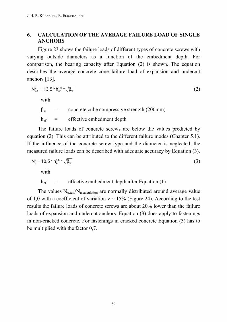
Figure 23 shows the failure loads of different types of concrete screws with
varying outside diameters as a function of the embedment depth. For
comparison, the bearing capacity after Equation (2) is shown. The equation
describes the average concrete cone failure load of expansion and undercut
anchors [13].
w
1,5
ef
0
u.c *h*13,5 β=N (2)
with
くw = concrete cube compressive strength (200mm)
hef = effective embedment depth
The failure loads of concrete screws are below the values predicted by
equation (2). This can be attributed to the different failure modes (Chapter 5.1).
If the influence of the concrete screw type and the diameter is neglected, the
measured failure loads can be described with adequate accuracy by Equation (3).
w
1,5
ef
0
u *h*10,5 β=N (3)
with
hef = effective embedment depth after Equation (1)
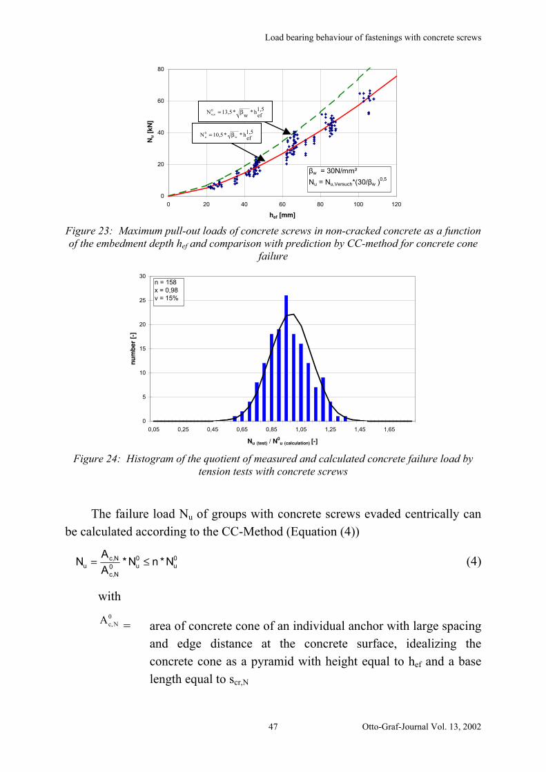
The values Nu,test/Nu,calculation are normally distributed around average value
of 1,0 with a coefficient of variation v ~ 15% (Figure 24). According to the test
results the failure loads of concrete screws are about 20% lower than the failure
loads of expansion and undercut anchors. Equation (3) does apply to fastenings
in non-cracked concrete. For fastenings in cracked concrete Equation (3) has to
be multiplied with the factor 0,7.
46
Load bearing behaviour of fastenings with concrete screws
0
20
40
60
80
0 20 40 60 80 100 120
hef [mm]
Nu [
kN
]
くw = 30N/mm²
Nu = Nu,Versuch*(30/くw )0,5
1,5ef
h*w
*13,5N 0cu, β=
1,5ef
h**10,5N w0u β=
Figure 23: Maximum pull-out loads of concrete screws in non-cracked concrete as a function
of the embedment depth hef and comparison with prediction by CC-method for concrete cone
failure
0
5
10
15
20
25
30
0,05 0,25 0,45 0,65 0,85 1,05 1,25 1,45 1,65
Nu (test) / N0u (calculation) [-]
nu
mb
er
[-]
n = 158
x = 0,98
v = 15%
Figure 24: Histogram of the quotient of measured and calculated concrete failure load by
tension tests with concrete screws
The failure load Nu of groups with concrete screws evaded centrically can
be calculated according to the CC-Method (Equation (4))
0
u
0
u0
Nc,
Nc,
u N*nN*A
A≤=N (4)
with
0Nc,A = area of concrete cone of an individual anchor with large spacing
and edge distance at the concrete surface, idealizing the
concrete cone as a pyramid with height equal to hef and a base
length equal to scr,N
Otto-Graf-Journal Vol. 13, 2002 47

J. H. R. KÜENZLEN, R. ELIGEHAUSEN
Ac,N = actual area of concrete cone of the anchorage at the concrete
surface. It is limited by overlapping concrete cones of adjoining
anchors (s ø scr,N) as well as by edges of the concrete member (c
ø ccr,N). Examples for the calculation of Ac,N are given in [14,
15]
N = number of anchors of the group
For expansion and undercut anchors the critical anchor spacing is scr,N =
3hef ([14, 15]). The failure load of concrete screws at the same embedment depth
is lower than that of expansion and undercut anchors. However, Figure 22 shows
that the test results can be described approximately with scr,N = 3 hef.
7. DESIGN OF FASTENINGS WITH CONCRETE SCREWS THAT MEET TECHNICAL APPROVALS
In references [1] to [3] the design of fastenings with concrete screws takes
place according to design method A in [16], which is based on the CC-Method.
The characteristic values necessary for the design of fastenings with concrete
screws with d0 = 10mm under tension load are assembled in Table 1. The high
characteristic resistance NRk,s at steel failure cannot be exploited because it is
higher than the characteristic resistance NRk,p at pullout. The values NRk,p were
determined from the tests for the technical approvals. The behaviour of the
fastening in cracks with opening and closing crack widths was considered as
well. The design at the failure mode “concrete cone failure” takes place
according to the CC-Method for expansion and undercut anchors which is
described in detail in [14, 15].
For consideration of the lower load capacity of concrete screws in
comparison to expansion and undercut anchors in Equation (5) a reduced
embedment depth hef,cal, in comparison to equation (1), is used to calculate the
characteristic resistance against concrete cone failure for a single concrete
screw. The embedment depths used are stated in Table 1.
wWN
1,5
calef,
0
cu, **h*7,0 ψβ=N (5)
with
くWN = nominal value of the cube strength after DIN 1045 [17]
hef,cal = nominal effective embedment depth (Table 1)
ねW = 1,0 for fastenings in cracked concrete
= 1,4 for fastenings in non-cracked concrete 48

Load bearing behaviour of fastenings with concrete screws
Table 1: Characteristic values for the resistances under tension load of concrete screws
(d0 = 10mm) with a Technical Approval of the DIBt
Type of concrete screw [1] [2] [3]
Drill hole diameter d0 [mm] 10 10 10
Embedment depth hnom [mm] 70 75 85
Steel failure
Characteristic resistance NRk,s [kN] 54,1 75,4 58
Pull-out failure
Characteristic resistance in non-cracked concrete B 25
NRk,p [kN] 12,0 16,0 20,0
Characteristic resistance in cracked concrete B 2
NRk,p [kN] 7,5 12,0 12,0
Concrete cone failure
Nominal effective embedment depth
hef,cal [mm] 50 50 60
Characteristic screw spacing scr,N [mm] 150 150 180
Characteristic edge distance ccr,N [mm] 75 75 90
8. SUMMARY
Concrete screws are a relatively new fastening system. Their main
advantage compared to traditional post-installed fastening systems is a quick and
easy installation. A hole is drilled into the concrete and threads are cut in the
concrete by the screw as it is installed.
Concrete screws transfer tensile loads into the base material by mechanical
interlock of the threads. Due to their load-bearing mechanism, concrete screws
with a technical approval of the DIBt can be used for fastenings in cracked and
non-cracked concrete.
The typical failure mechanism for concrete screws is concrete-cone failure.
With increasing embedment depth the ratio of the depth of the concrete failure
cone to the embedment depth decreases. The failure load of concrete screws
with continuous threads along the entire embedment depth increases
proportionally to hef1,5 (hef = effective embedment depth), but it is about 20 %
Otto-Graf-Journal Vol. 13, 2002 49
J. H. R. KÜENZLEN, R. ELIGEHAUSEN
smaller than the failure load of expansion and undercut anchors with the same
embedment depth.
In order for concrete screws to function properly, the threads cut into the
wall of the drilled hole must not be damaged during the installation. This
requirement is achieved by using the embedment depth defined in the Technical
Approvals.
9. ACKNOWLEDGMENT
The primary funding for this research was provided by the Adolf Würth
GmbH & Co. KG. The support of this manufacturer is very much appreciated.
Special thanks are also accorded to Beate Vladika and Matthew Hoehler who
spent many hours in improving the English.
10. REFERENCES
[1] [Deutsches Institut für Bautechnik] Allgemeine Bauaufsichtliche
Zulassung Z-21.1-1712 für Hilti Schraubanker HUS-H zur Verankerung
im gerissenen und ungerissenen Beton, Berlin, 2001
[2] [Deutsches Institut für Bautechnik] Allgemeine Bauaufsichtliche
Zulassung Z-21.1-1549 für HECO-MULTI-MONTI-Schraubanker MMS
zur Verankerung im gerissenen und ungerissenen Beton, Berlin, 2001
[3] [Deutsches Institut für Bautechnik] Allgemeine Bauaufsichtliche
Zulassung Z-21.1-1624 für Toge Betonschraube TSM zur Verankerung
im gerissenen und ungerissenen Beton, Berlin, 2001
[4] European Organisation for Technical Approvals (EOTA): Leitlinie für die
europäisch-technische Zulassung von Metalldübeln zur Verankerung in
Beton. Deutsches Institut für Bautechnik, 28. Jahrgang, Sonderheft Nr. 16,
Berlin, Dezember 1997
[5] Küenzlen, J. H. R.; Eligehausen, R.: Setz- und Ausziehversuche in
ungerissenem Beton mit Schraubdübeln. Bericht Nr. AF01/01-E00202/1,
Institut für Werkstoffe im Bauwesen, Universität Stuttgart, 2001, nicht
veröffentlicht
[6] Küenzlen, J. H. R.; Eligehausen, R.: Tragverhalten von Schraubdübeln in
niederfestem Beton. Bericht Nr. W8/1-01/1, Institut für Werkstoffe im
Bauwesen, Universität Stuttgart, 2001, nicht veröffentlicht
50

Load bearing behaviour of fastenings with concrete screws
[7] Küenzlen, J. H. R.; Eligehausen, R.: Tragverhalten von Schraubdübeln in
niederfestem Beton. Bericht Nr. W8/3-01/3, Institut für Werkstoffe im
Bauwesen, Universität Stuttgart, 2001, nicht veröffentlicht
[8] Küenzlen, J. H. R.; Eligehausen, R.: Einfluss verschiedener Parameter auf
die Höchstlasten von Schraubdübeln, Institut für Werkstoffe im
Bauwesen, Universität Stuttgart, 2001, Bericht in Vorbereitung
[9] Küenzlen, J. H. R.; Sippel, T. M.: Behaviour and Design of Fastenings
with Concrete Screws. In: RILEM Proceedings PRO 21 „Symposium on
Connections between Steel and Concrete“, Cachan Cedex, 2001, S. 919-
929.
[10] Küenzlen, J. H. R.: Drehmomentversuche mit Schraubdübeln in
ungerissenem Beton. Jahresbericht 2000/2001, Institut für Werkstoffe im
Bauwesen, Universität Stuttgart, 2001
[11] Eligehausen, R.; Hofacker, I. N.; Spieth, H. A.; Küenzlen, J. H. R.: Neue
Entwicklungen in der Befestigungstechnik, Tagungsband, IBK-Bau-
Fachtagung 263: Dübel und Befestigungstechnik, 2000, S. 2.1-2.14,
[12] Meszaros, J.,: Tragverhalten von Einzelverbunddübeln unter zentrischer
Kurzzeitbelastung. Dissertation, Universität Stuttgart, 2001
[13] Eligehausen, R.; Fuchs, W.; Mayer, B.: Tragverhalten von
Dübelbefestigungen bei Zugbeanspruchung. Beton + Fertigteil-Technik
1987, Heft 12, S. 826-832 und 1988 Heft 1, S. 29-35.
[14] Eligehausen, R.; Mallée, R.: Befestigungstechnik im Beton- und
Mauerwerkbau. Ernst & und Sohn, Berlin, 2000.
[15] Fuchs, W.; Eligehausen, R.: Das CC-Verfahren zur Berechnung der
Betonausbruchlast von Verankerungen. Beton- und Stahlbetonbau, 1995,
Heft 1, S. 6-9, Heft 2, S. 38-44, Heft 3, S. 73-76.
[16] Deutsches Institut für Bautechnik: Bemessungsverfahren für Dübel zur
Verankerung in Beton (Anhang zum Zulassungsbescheid). Berlin, 1993
[17] DIN 1045, Beton und Stahlbeton, Bemessung und Ausführung, Ausgabe
1978
Otto-Graf-Journal Vol. 13, 2002 51

J. H. R. KÜENZLEN, R. ELIGEHAUSEN
52

Prestressed hollow-core concrete slabs – Problems and possibilities in fastening techniques
PRESTRESSED HOLLOW-CORE CONCRETE SLABS – PROBLEMS AND POSSIBILITIES IN FASTENING TECHNIQUES
SPANNBETON-HOHLDECKENPLATTEN – PROBLEME UND MÖG-LICHKEITEN IN DER BEFESTIGUNGSTECHNIK
DALLES ALVEOLAIRES EN BÉTON PRÉCONTRAINT – PROBLÈ-MES ET POSSIBILITÉS DES TECHNIQUES D'ANCRAGE
Clemens Lutz
SUMMARY
In the present, prestressed hollow-cored concrete slabs are tendentiously
used as ceiling systems. Therefore, fastening techniques with regard to these
slabs gain in an increasing importance. In this article, advantages of these mem-
bers and problems by application of anchors are described, and different struc-
tural responses between several types of anchors are experimentally determined.
Accordingly, it seems to be essential to choose or to adapt suitable anchors for
ceiling systems.
ZUSAMMENFASSUNG
Spannbeton-Hohlplatten finden als Deckensystem eine immer breitere
Verwendung und einen immer größeren Anwendungsbereich. Somit gewinnt
auch eine korrekte Befestigung in diesen Platten zunehmend an Bedeutung. In
diesem Artikel wird auf die Vorteile der Platten, aber auch auf die Problematik,
die bei der Montage von Dübeln entstehen, eingegangen. Ferner wird gezeigt,
dass es große qualitative Unterschiede bezüglich der Tauglichkeit verschiedener
Befestigungssysteme gibt, weshalb eine sorgfältige Auswahl bzw. Anpassung
prinzipiell geeigneter Dübel stattfinden muss.
RESUME
Actuellement, les dalles alvéolaires en béton précontraint sont utilisées de
plus en plus fréquemment. Par conséquent, les ancrages appropriés gagnent
d'importance. Dans cet article, nous traitons les avantages de ces dalles et les
problèmes reliés à l'utilisation de chevilles. De plus, nous montrons que les dif-
Otto-Graf-Journal Vol. 13, 2002 53
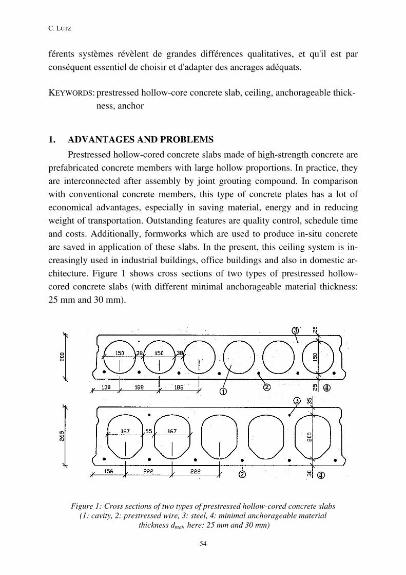
C. LUTZ
férents systèmes révèlent de grandes différences qualitatives, et qu'il est par
conséquent essentiel de choisir et d'adapter des ancrages adéquats.
KEYWORDS: prestressed hollow-core concrete slab, ceiling, anchorageable thick-
ness, anchor
1. ADVANTAGES AND PROBLEMS
Prestressed hollow-cored concrete slabs made of high-strength concrete are
prefabricated concrete members with large hollow proportions. In practice, they
are interconnected after assembly by joint grouting compound. In comparison
with conventional concrete members, this type of concrete plates has a lot of
economical advantages, especially in saving material, energy and in reducing
weight of transportation. Outstanding features are quality control, schedule time
and costs. Additionally, formworks which are used to produce in-situ concrete
are saved in application of these slabs. In the present, this ceiling system is in-
creasingly used in industrial buildings, office buildings and also in domestic ar-
chitecture. Figure 1 shows cross sections of two types of prestressed hollow-
cored concrete slabs (with different minimal anchorageable material thickness:
25 mm and 30 mm).
1
4
4
Figure 1: Cross sections of two types of prestressed hollow-cored concrete slabs (1: cavity, 2: prestressed wire, 3: steel, 4: minimal anchorageable material
thickness dmat, here: 25 mm and 30 mm)
54
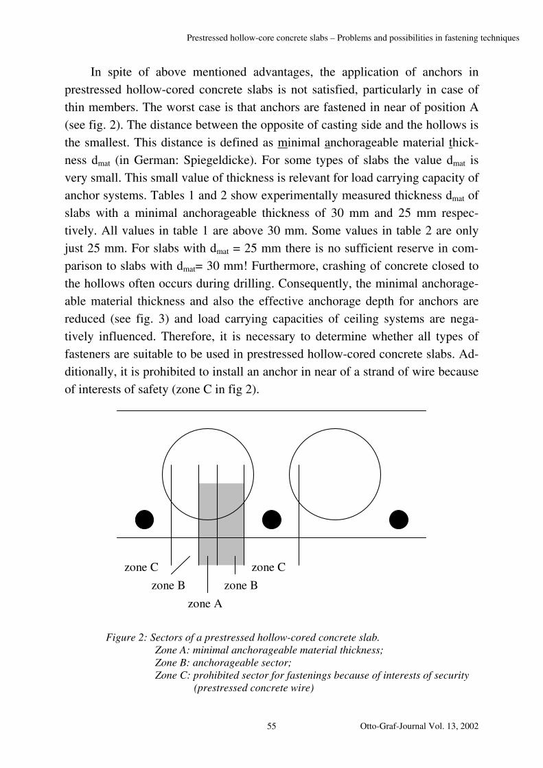
Prestressed hollow-core concrete slabs – Problems and possibilities in fastening techniques
In spite of above mentioned advantages, the application of anchors in
prestressed hollow-cored concrete slabs is not satisfied, particularly in case of
thin members. The worst case is that anchors are fastened in near of position A
(see fig. 2). The distance between the opposite of casting side and the hollows is
the smallest. This distance is defined as minimal anchorageable material thick-
ness dmat (in German: Spiegeldicke). For some types of slabs the value dmat is
very small. This small value of thickness is relevant for load carrying capacity of
anchor systems. Tables 1 and 2 show experimentally measured thickness dmat of
slabs with a minimal anchorageable thickness of 30 mm and 25 mm respec-
tively. All values in table 1 are above 30 mm. Some values in table 2 are only
just 25 mm. For slabs with dmat = 25 mm there is no sufficient reserve in com-
parison to slabs with dmat= 30 mm! Furthermore, crashing of concrete closed to
the hollows often occurs during drilling. Consequently, the minimal anchorage-
able material thickness and also the effective anchorage depth for anchors are
reduced (see fig. 3) and load carrying capacities of ceiling systems are nega-
tively influenced. Therefore, it is necessary to determine whether all types of
fasteners are suitable to be used in prestressed hollow-cored concrete slabs. Ad-
ditionally, it is prohibited to install an anchor in near of a strand of wire because
of interests of safety (zone C in fig 2).
zone B
zone C zone C
zone A
zone B
Figure 2: Sectors of a prestressed hollow-cored concrete slab. Zone A: minimal anchorageable material thickness; Zone B: anchorageable sector; Zone C: prohibited sector for fastenings because of interests of security (prestressed concrete wire)
Otto-Graf-Journal Vol. 13, 2002 55

C. LUTZ
Table 1: measured values dmat (slab with a minimal anchorageable thickness of 30 mm)
39,6 42,3
43,1 44,2
42,3 45,0
40,9 43,8
dmat [mm] (measured mini-
mal anchorageable material
thickness)
37,8 39,2
Range [mm] 38 (>30) to 45
Average [mm] 41,8
Variation coeff. [%] 5,70
Table 2: measured values dmat (slab with a minimal anchorageable thickness of 25 mm)
25,1 26,7
26,7 28,5
27,6 28,5
26,8 27,5
26,2 28,6
dmat [mm] (measured mini-
mal anchorageable material
thickness)
25,0 26,1
Range [mm] 25 to 29
Average [mm] 26,9
Variation coeff. [%] 4,60
dmat dmat, eff
Figure 3: The minimal anchorageable material thickness dmat after drilling is reduced (:=dmat, eff < dmat).
56
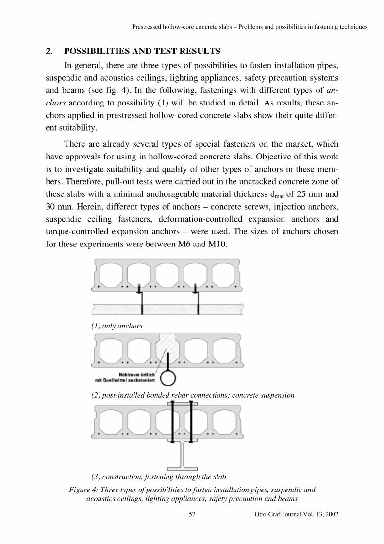
Prestressed hollow-core concrete slabs – Problems and possibilities in fastening techniques
2. POSSIBILITIES AND TEST RESULTS
In general, there are three types of possibilities to fasten installation pipes,
suspendic and acoustics ceilings, lighting appliances, safety precaution systems
and beams (see fig. 4). In the following, fastenings with different types of an-
chors according to possibility (1) will be studied in detail. As results, these an-
chors applied in prestressed hollow-cored concrete slabs show their quite differ-
ent suitability.
There are already several types of special fasteners on the market, which
have approvals for using in hollow-cored concrete slabs. Objective of this work
is to investigate suitability and quality of other types of anchors in these mem-
bers. Therefore, pull-out tests were carried out in the uncracked concrete zone of
these slabs with a minimal anchorageable material thickness dmat of 25 mm and
30 mm. Herein, different types of anchors – concrete screws, injection anchors,
suspendic ceiling fasteners, deformation-controlled expansion anchors and
torque-controlled expansion anchors – were used. The sizes of anchors chosen
for these experiments were between M6 and M10.
(1) only anchors
(2) post-installed bonded rebar connections; concrete suspension
(3) construction, fastening through the slab
Figure 4: Three types of possibilities to fasten installation pipes, suspendic and acoustics ceilings, lighting appliances, safety precaution and beams
Otto-Graf-Journal Vol. 13, 2002 57
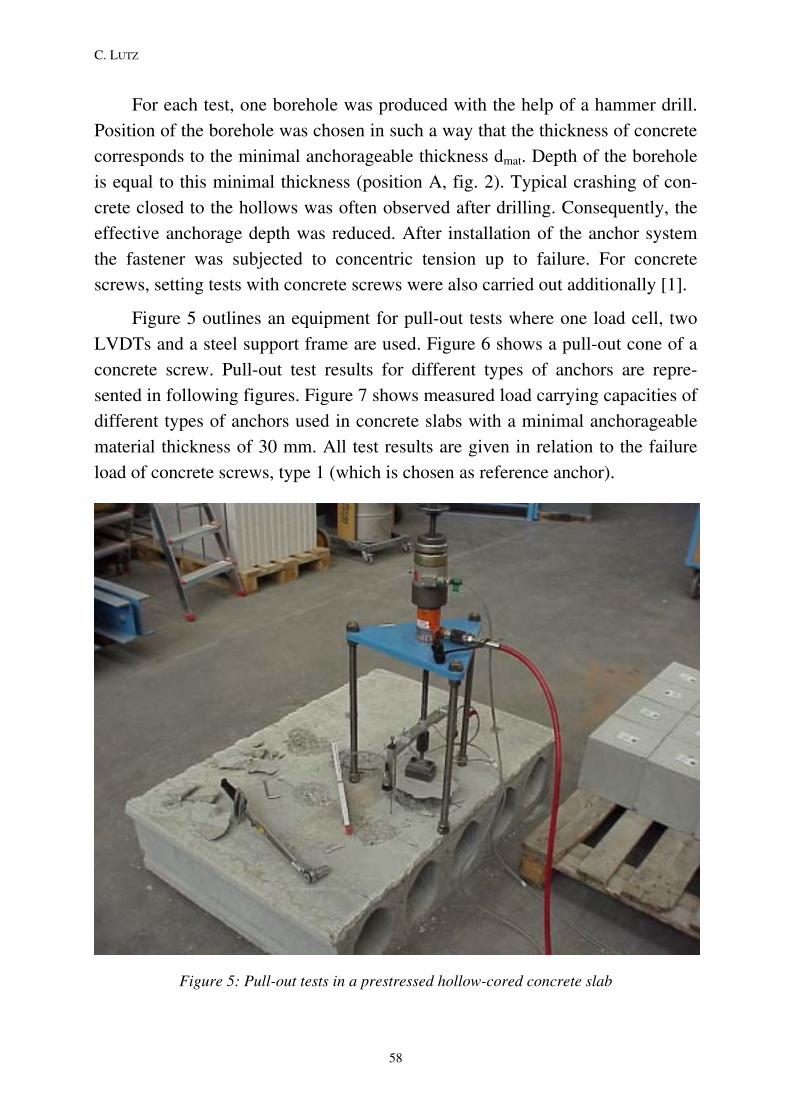
C. LUTZ
For each test, one borehole was produced with the help of a hammer drill.
Position of the borehole was chosen in such a way that the thickness of concrete
corresponds to the minimal anchorageable thickness dmat. Depth of the borehole
is equal to this minimal thickness (position A, fig. 2). Typical crashing of con-
crete closed to the hollows was often observed after drilling. Consequently, the
effective anchorage depth was reduced. After installation of the anchor system
the fastener was subjected to concentric tension up to failure. For concrete
screws, setting tests with concrete screws were also carried out additionally [1].
Figure 5 outlines an equipment for pull-out tests where one load cell, two
LVDTs and a steel support frame are used. Figure 6 shows a pull-out cone of a
concrete screw. Pull-out test results for different types of anchors are repre-
sented in following figures. Figure 7 shows measured load carrying capacities of
different types of anchors used in concrete slabs with a minimal anchorageable
material thickness of 30 mm. All test results are given in relation to the failure
load of concrete screws, type 1 (which is chosen as reference anchor).
Figure 5: Pull-out tests in a prestressed hollow-cored concrete slab
58
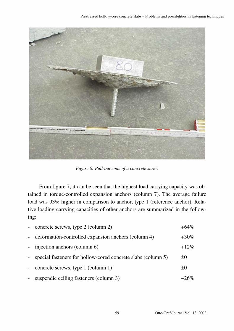
Prestressed hollow-core concrete slabs – Problems and possibilities in fastening techniques
Figure 6: Pull-out cone of a concrete screw
From figure 7, it can be seen that the highest load carrying capacity was ob-
tained in torque-controlled expansion anchors (column 7). The average failure
load was 93% higher in comparison to anchor, type 1 (reference anchor). Rela-
tive loading carrying capacities of other anchors are summarized in the follow-
ing:
- concrete screws, type 2 (column 2) +64%
- deformation-controlled expansion anchors (column 4) +30%
- injection anchors (column 6) +12%
- special fasteners for hollow-cored concrete slabs (column 5) ±0
- concrete screws, type 1 (column 1) ±0
- suspendic ceiling fasteners (column 3) −26%
Otto-Graf-Journal Vol. 13, 2002 59
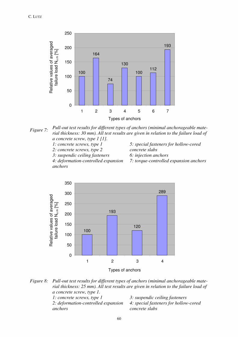
100
164
74
130
100112
193
0
50
100
150
200
250
1 2 3 4 5 6 7
Dübelart
Nu
,m [
%]
Types of anchors
Re
lative
va
lue
s o
f a
ve
rag
ed
fa
ilure
lo
ad
Nu.m
[%
]
C. LUTZ
Pull-out test results for different types of anchors (minimal anchorageable mate-rial thickness: 30 mm). All test results are given in relation to the failure load of a concrete screw, type 1 [1].
Figure 7:
1: concrete screws, type 1 2: concrete screws, type 2 3: suspendic ceiling fasteners 4: deformation-controlled expansion anchors
5: special fasteners for hollow-cored concrete slabs 6: injection anchors 7: torque-controlled expansion anchors
100
193
120
289
0
50
100
150
200
250
300
350
1 2 3 4
Dübelart
Nu
,m [
%]
Re
lative
va
lue
s o
f a
ve
rag
ed
fa
ilure
lo
ad
Nu.m
[%
]
Types of anchors
Pull-out test results for different types of anchors (minimal anchorageable mate-rial thickness: 25 mm). All test results are given in relation to the failure load of a concrete screw, type 1.
Figure 8:
1: concrete screws, type 1 2: deformation-controlled expansion anchors
3: suspendic ceiling fasteners 4: special fasteners for hollow-cored concrete slabs
60
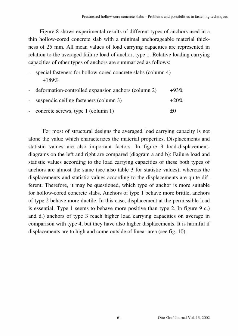
Prestressed hollow-core concrete slabs – Problems and possibilities in fastening techniques
Figure 8 shows experimental results of different types of anchors used in a
thin hollow-cored concrete slab with a minimal anchorageable material thick-
ness of 25 mm. All mean values of load carrying capacities are represented in
relation to the averaged failure load of anchor, type 1. Relative loading carrying
capacities of other types of anchors are summarized as follows:
- special fasteners for hollow-cored concrete slabs (column 4)
+189%
- deformation-controlled expansion anchors (column 2) +93%
- suspendic ceiling fasteners (column 3) +20%
- concrete screws, type 1 (column 1) ±0
For most of structural designs the averaged load carrying capacity is not
alone the value which characterizes the material properties. Displacements and
statistic values are also important factors. In figure 9 load-displacement-
diagrams on the left and right are compared (diagram a and b): Failure load and
statistic values according to the load carrying capacities of these both types of
anchors are almost the same (see also table 3 for statistic values), whereas the
displacements and statistic values according to the displacements are quite dif-
ferent. Therefore, it may be questioned, which type of anchor is more suitable
for hollow-cored concrete slabs. Anchors of type 1 behave more brittle, anchors
of type 2 behave more ductile. In this case, displacement at the permissible load
is essential. Type 1 seems to behave more positive than type 2. In figure 9 c.)
and d.) anchors of type 3 reach higher load carrying capacities on average in
comparison with type 4, but they have also higher displacements. It is harmful if
displacements are to high and come outside of linear area (see fig. 10).
Otto-Graf-Journal Vol. 13, 2002 61

C. LUTZ
displacement
load
displacement
load
a.) type 1
b.) type 2
displacement
load
displacement
loa
d
c.) type 3 d.) type 4
0 0 sx sx
Nx Nx
0 0
sy sy
Ny Ny
0 0
0 0
Figure 9: Load-displacement-curves for different types of anchors. Diagrams a.) and b.): Difference in displacement with almost the same failure load.
Diagrams c.) and d.): Difference in failure load and displacement
Table 3: Statistic values of two types of anchors in a prestressed hollow-cored concrete slab with dmat= 30 mm (see figure 9)
a.) Type 1 b.) Type 2 Variation coefficient at failure load Nu,m [%] 17 17
Displacement at 0,5 Nu,m [%] 100 560
Variation coefficient for displacement at 0,5 Nu,m [%] 11 25
62

Prestressed hollow-core concrete slabs – Problems and possibilities in fastening techniques
Obviously, the load carrying capacity is not only the aspect characterizing
anchors. In principle, three groups of anchors could be distinguished according
to their load-displacement-behaviours (see fig. 11):
- Group 1: anchors with little displacements, i.e. the tested injection anchors.
- Group 2: anchors with larger displacements and high load carrying capaci-
ties, i. e. one of the tested torque-controlled expansion anchors.
- Group 3: anchors with larger displacements and reduced load carrying ca-
pacities.
0 0.5 1 1.5 2
Displacement s [mm]
Loa
d N
Linear-elastic
area
Linear-elastic area
Figure 10: Experimental load-displacement-curves and simplified linear curves for two types of anchors in a prestressed hollow-cored concrete slab (here: with dmat= 30 mm).
Otto-Graf-Journal Vol. 13, 2002 63
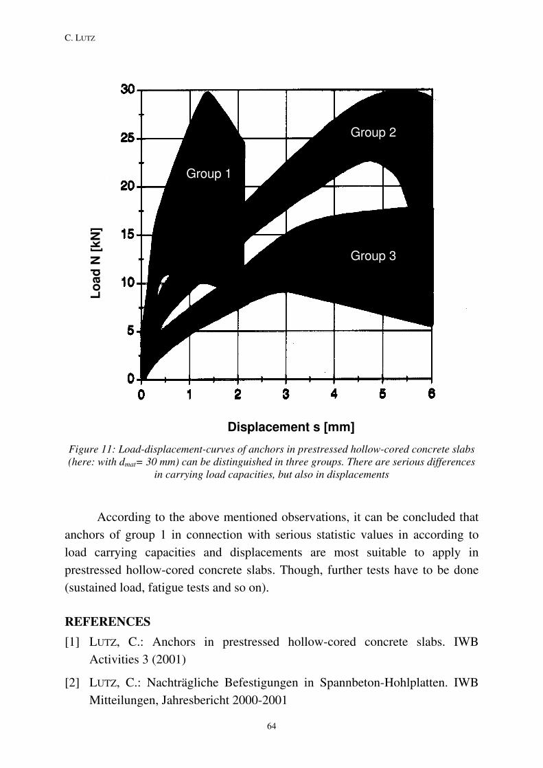
C. LUTZ
Group 1
Group 2
Group 3
Displacement s [mm]
Figure 11: Load-displacement-curves of anchors in prestressed hollow-cored concrete slabs (here: with dmat= 30 mm) can be distinguished in three groups. There are serious differences
in carrying load capacities, but also in displacements
Lo
ad
N [
kN
]
According to the above mentioned observations, it can be concluded that
anchors of group 1 in connection with serious statistic values in according to
load carrying capacities and displacements are most suitable to apply in
prestressed hollow-cored concrete slabs. Though, further tests have to be done
(sustained load, fatigue tests and so on).
REFERENCES
[1] LUTZ, C.: Anchors in prestressed hollow-cored concrete slabs. IWB
Activities 3 (2001)
[2] LUTZ, C.: Nachträgliche Befestigungen in Spannbeton-Hohlplatten. IWB
Mitteilungen, Jahresbericht 2000-2001
64

Pore-size determination from penetration tests on concrete with n-decane
PORE-SIZE DETERMINATION FROM PENETRATION TESTS ON CONCRETE WITH N-DECANE
PORENGRÖSSENBESTIMMUNG AUS N-DECAN-EINDRING-VERSUCHEN IN BETON
DETERMINATION DES PORES DU A LA PENETRATION DE N-DECANE EN BETON
Hans W. Reinhardt, Arno Pfingstner
SUMMARY
Absorption and infiltration tests on concrete mixes have been carried out
with n-decane. The test results show a good agreement with theoretical predic-
tions. The results indicate that the main parameter on the penetration is the wa-
ter-cement ratio. Pore sizes which are reached are different for the absorption
test and the infiltration test.
ZUSAMMENFASSUNG
Absorptions- und Infiltrationsversuche wurden an verschiedenen Betonen
mit n-Decan durchgeführt. Die Ergebnisse haben eine gute Übereinstimmung
mit theoretischen Vorhersagen gezeigt. Die Ergebnisse lassen den Schluss zu,
dass der Wasserzementwert die maßgebliche Größe für das Eindringverhalten
ist. Porengrößen, die erreicht wurden, sind bei Absorptions- und Infiltrationsver-
suchen verschieden.
RESUME
Des essais d'absorption et d'infiltration ont été réalisés sur des bétons de
différentes compositions avec du n-décane. Les résultats montrent une bonne
concordance avec des prévisions théoriques. Les résultats indiquent que le pa-
ramètre principal pour la pénétration dans le béton est le rapport eau-ciment. Les
tailles des pores atteintes sont différentes pour les essais d'absorption et les es-
sais d'infiltration.
KEYWORDS: Concrete, n-decane, penetration, absorption, infiltration, high-
performance concrete
Otto-Graf-Journal Vol. 13, 2002 65

H.W. REINHARDT, A. PFINGSTNER
MOTIVE
Since several years, tests have been carried out on the penetration behav-
iour of organic fluids in concrete [1-5]. Two types of tests are being carried out:
the capillary suction test and the infiltration test with a certain hydraulic head.
The test results show that the capillary suction test satisfies usually technical
requirements for the application of the material properties in assessing the be-
haviour of real structures. However, from a scientific point of view both tests
reveal more than the material property only. Comparing the test results of both
test methods one can calculate the pore radius of capillary pores in concrete.
This will be shown in the following.
EXPERIMENTAL SET UP
For suction tests, specimens were placed into the test fluid. The samples
rested on glass rods to allow free access of the testing fluid to the inflow surface.
The fluid level was approx. 10 mm above the lower end of the specimen. Pene-
tration occurred by capillary forces acting against gravity.
The experimental set-up for infiltration tests described in DAfStb guide-
line [6] was slightly modified. Preliminary tests had proven that the pressure
head of 40 (+/- 5) cm specified there was too small to obtain measurable differ-
ences to capillary suction tests for high performance concretes. The required ex-
ternal pressure was estimated by calculation from the pore radius distributions of
comparable concretes and fixed to 0,2 bar (20 kN/m2) for all infiltration tests.
This pressure was produced by a nitrogen bottle connected to the funnels on the
samples by tubes.
66
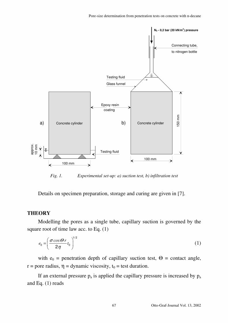
Pore-size determination from penetration tests on concrete with n-decane
100 mm
150 m
m
Concrete cylinder
Glass funnel
Connecting tube,
Testing fluid
to nitrogen bottle
N2 - 0,2 bar (20 kN/m2) pressure
100 mm
Concrete cylinder
Epoxy resin
coating
appro
x.
10 m
m
Testing fluid
a) b)
Fig. 1. Experimental set-up: a) suction test, b) infiltration test
Details on specimen preparation, storage and curing are given in [7].
THEORY
Modelling the pores as a single tube, capillary suction is governed by the
square root of time law acc. to Eq. (1)
1 2
02
/cos r
eσ Θ
η
Ã= ÄÅ Ö
0tÔÕ (1)
with e0 = penetration depth of capillary suction test, Θ = contact angle,
r = pore radius, η = dynamic viscosity, t0 = test duration.
If an external pressure pa is applied the capillary pressure is increased by pa
and Eq. (1) reads
Otto-Graf-Journal Vol. 13, 2002 67
H.W. REINHARDT, A. PFINGSTNER
1 222
4
/
p a
cos re p
r
σ Θ
η
ÃÃ Ô= +ÄÄ Õ
Å ÖÅ ÖptÔÕ (2)
with ep = penetration test of infiltration test, tp = test duration. When Eqs.
(1) and (2) are divided by each other one gets
2
0
0
21
p
p a
e t cosr
e t p
σ ΘÃ ÔÃ ÔÄ Õ= −Ä ÕÄ ÕÅ ÖÅ Ö
(3)
Eq. (3) is an explicit equation for the effective pore radius. The effective
pore radius is a fictitious pore size which is related to the single size pore model,
i. e. concrete consists only of parallel pores of this size. Of course this model is a
simplistic one since pores of many sizes take part in the capillary suction which
depends on the pore size distribution of concrete. Studying the effective pore
radius one should carry out experiments of short and long duration, during
which readings are taken. However, in the following experiments only meas-
urements after 72 hours are taken and the results explain the way of evaluation.
Eq. (3) can be written in a different way when the penetration coefficient
B = e t -1/2 has already been evaluated. Eq. (3) becomes
2
0
21
p
a
B cosr
B p
σ ΘÃ ÔÃ ÔÄ Õ= −Ä ÕÄ ÕÅ ÖÅ Ö
(4)
with the index 0 referring to the suction test and p to the infiltration test.
A similar relation can be derived if the sorptivity S is used instead of the
penetration coefficient B. S is linked to B via the porosity ε
S B ε= ⋅ (5)
with ε = const. Eq. (4) becomes
2
0
21
p
a
S cosr
S p
σ ΘÃ ÔÃ ÔÄ Õ= −Ä ÕÄ ÕÅ ÖÅ Ö
.
68
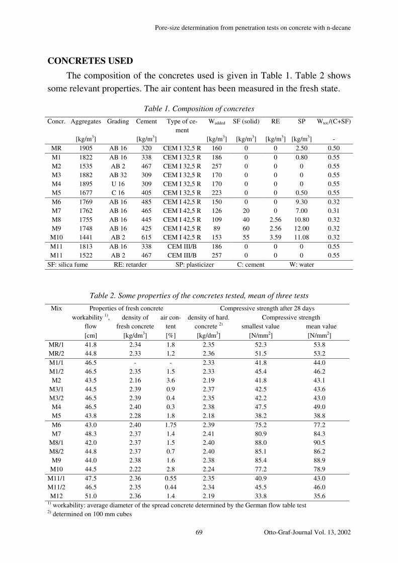
Pore-size determination from penetration tests on concrete with n-decane
CONCRETES USED
The composition of the concretes used is given in Table 1. Table 2 shows
some relevant properties. The air content has been measured in the fresh state.
Table 1. Composition of concretes
Concr. Aggregates
[kg/m3]
Grading Cement
[kg/m3]
Type of ce-
ment
Wadded
[kg/m3]
SF (solid)
[kg/m3]
RE
[kg/m3]
SP
[kg/m3]
Wtot./(C+SF)
-
MR 1905 AB 16 320 CEM I 32,5 R 160 0 0 2.50 0.50
M1 1822 AB 16 338 CEM I 32,5 R 186 0 0 0.80 0.55
M2 1535 AB 2 467 CEM I 32,5 R 257 0 0 0 0.55
M3 1882 AB 32 309 CEM I 32,5 R 170 0 0 0 0.55
M4 1895 U 16 309 CEM I 32,5 R 170 0 0 0 0.55
M5 1677 C 16 405 CEM I 32,5 R 223 0 0 0.50 0.55
M6 1769 AB 16 485 CEM I 42,5 R 150 0 0 9.30 0.32
M7 1762 AB 16 465 CEM I 42,5 R 126 20 0 7.00 0.31
M8 1755 AB 16 445 CEM I 42,5 R 109 40 2.56 10.80 0.32
M9 1748 AB 16 425 CEM I 42,5 R 89 60 2.56 12.00 0.32
M10 1441 AB 2 615 CEM I 42,5 R 153 55 3.59 11.08 0.32
M11 1813 AB 16 338 CEM III/B 186 0 0 0 0.55
M11 1522 AB 2 467 CEM III/B 257 0 0 0 0.55
SF: silica fume RE: retarder SP: plasticizer C: cement W: water
Table 2. Some properties of the concretes tested, mean of three tests
Properties of fresh concrete Compressive strength after 28 days
workability 1),
flow
density of
fresh concrete
air con-
tent
density of hard.
concrete 2)
Compressive strength
smallest value mean value
Mix
[cm] [kg/dm3] [%] [kg/dm3] [N/mm2] [N/mm2]
MR/1 41.8 2.34 1.8 2.35 52.3 53.8
MR/2 44.8 2.33 1.2 2.36 51.5 53.2
M1/1 46.5 - - 2.33 41.8 44.0
M1/2 46.5 2.35 1.5 2.33 45.4 46.2
M2 43.5 2.16 3.6 2.19 41.8 43.1
M3/1 44.5 2.39 0.9 2.37 42.5 43.6
M3/2 46.5 2.39 0.4 2.35 42.2 43.0
M4 46.5 2.40 0.3 2.38 47.5 49.0
M5 43.8 2.28 1.8 2.18 38.2 38.8
M6 43.0 2.40 1.75 2.39 75.2 77.2
M7 48.3 2.37 1.4 2.41 80.9 84.3
M8/1 42.0 2.37 1.5 2.40 88.0 90.5
M8/2 44.8 2.37 0.7 2.40 85.1 86.2
M9 44.0 2.38 1.6 2.38 85.4 88.9
M10 44.5 2.22 2.8 2.24 77.2 78.9
M11/1 47.5 2.36 0.55 2.35 40.9 43.0
M11/2 46.5 2.35 0.44 2.34 45.5 46.0
M12 51.0 2.36 1.4 2.19 33.8 35.6 1) workability: average diameter of the spread concrete determined by the German flow table test 2) determined on 100 mm cubes
Otto-Graf-Journal Vol. 13, 2002 69
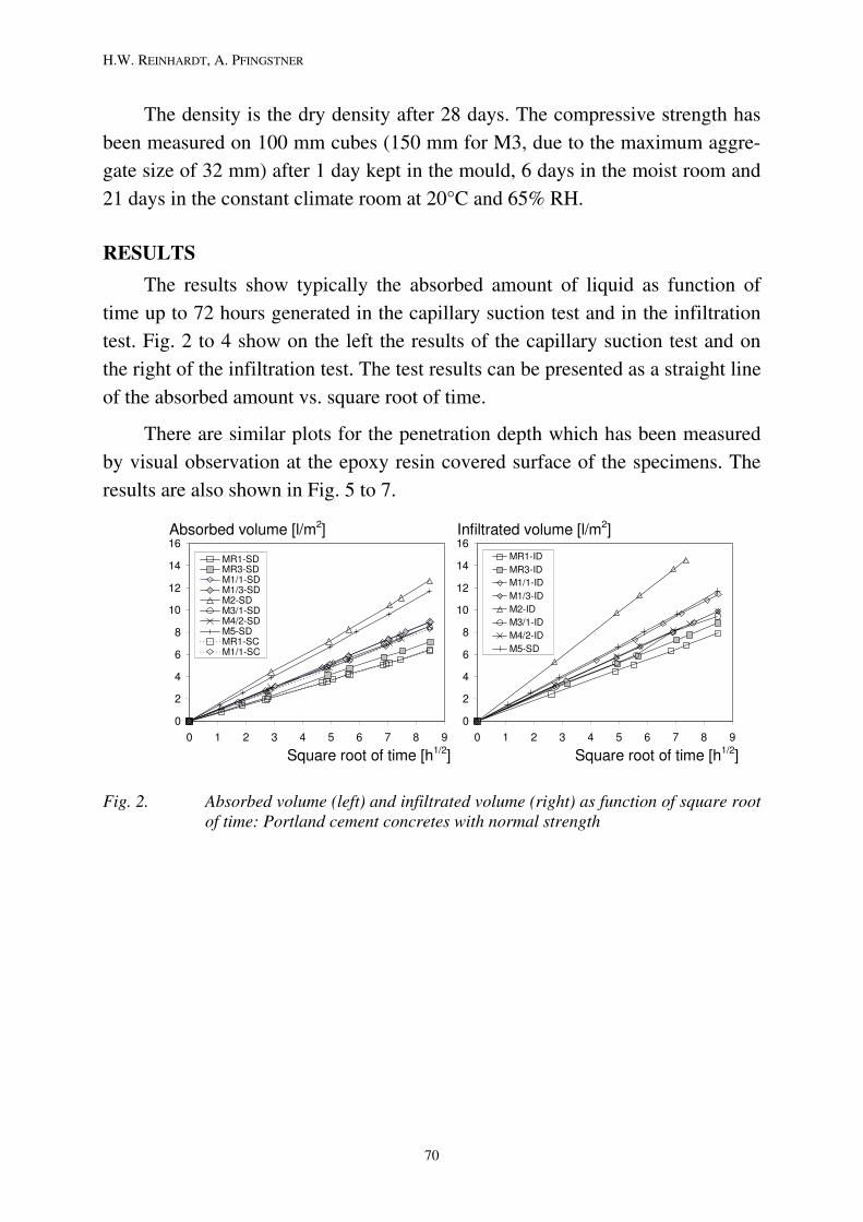
H.W. REINHARDT, A. PFINGSTNER
The density is the dry density after 28 days. The compressive strength has
been measured on 100 mm cubes (150 mm for M3, due to the maximum aggre-
gate size of 32 mm) after 1 day kept in the mould, 6 days in the moist room and
21 days in the constant climate room at 20°C and 65% RH.
RESULTS
The results show typically the absorbed amount of liquid as function of
time up to 72 hours generated in the capillary suction test and in the infiltration
test. Fig. 2 to 4 show on the left the results of the capillary suction test and on
the right of the infiltration test. The test results can be presented as a straight line
of the absorbed amount vs. square root of time.
There are similar plots for the penetration depth which has been measured
by visual observation at the epoxy resin covered surface of the specimens. The
results are also shown in Fig. 5 to 7.
0
2
4
6
8
10
12
14
16
0 1 2 3 4 5 6 7 8
Square root of time [h1
9/2]
MR1-SDMR3-SDM1/1-SDM1/3-SDM2-SDM3/1-SDM4/2-SDM5-SDMR1-SCM1/1-SC
Absorbed volume [l/m2]
0
2
4
6
8
10
12
14
16
0 1 2 3 4 5 6 7 8
Square root of time [h1
9/2]
MR1-ID
MR3-ID
M1/1-ID
M1/3-ID
M2-ID
M3/1-ID
M4/2-ID
M5-SD
Infiltrated volume [l/m2]
Fig. 2. Absorbed volume (left) and infiltrated volume (right) as function of square root of time: Portland cement concretes with normal strength
70
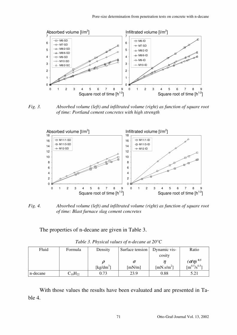
Pore-size determination from penetration tests on concrete with n-decane
0
1
2
3
4
5
6
7
0 1 2 3 4 5 6 7 8
Square root of time [h1
9/2]
M6-SD
M7-SD
M8/2-SD
M8/6-SD
M9-SD
M10-SD
M8/2-SC
Absorbed volume [l/m2]
0
1
2
3
4
5
6
7
0 1 2 3 4 5 6 7 8
Square root of time [h1
9/2]
M6-ID
M7-SD
M8/2-ID
M8/6-ID
M9-ID
M10-ID
Infiltrated volume [l/m2]
Fig. 3. Absorbed volume (left) and infiltrated volume (right) as function of square root of time: Portland cement concretes with high strength
0
2
4
6
8
10
12
14
16
18
0 1 2 3 4 5 6 7 8
Square root of time [h1
9/2]
M11/1-SD
M11/3-SD
M12-SD
Absorbed volume [l/m2]
0
2
4
6
8
10
12
14
16
18
0 1 2 3 4 5 6 7 8
Square root of time [h1
9/2]
M11/1-ID
M11/3-ID
M12-ID
Infiltrated volume [l/m2]
Fig. 4. Absorbed volume (left) and infiltrated volume (right) as function of square root of time: Blast furnace slag cement concretes
The properties of n-decane are given in Table 3.
Table 3. Physical values of n-decane at 20°C
Fluid Formula Density Surface tension Dynamic vis-
cosity
Ratio
( / ) 0.5
[kg/dm3] [mN/m] [mN.s/m2] [m0.5/s0.5]
n-decane C10H22 0.73 23.9 0.88 5.21
With those values the results have been evaluated and are presented in Ta-
ble 4.
Otto-Graf-Journal Vol. 13, 2002 71

H.W. REINHARDT, A. PFINGSTNER
Table 4. Pore parameters calculated from test results with n-decane
Sorptivity
l m-2 h-1/2
penetration coefficient
mm h-1/2
r, from B
µm
cos θ =
r, from S
µm
cos θ =
Concrete
So Sp Bo Bp 1 2/π 1 2/π
MR 0.750 0.931 10.5 12.1 0.79 0.50 1.29 0.82
M1 1.054 1.342 12.2 14.7 1.10 0.70 1.48 0.94
M2 1.491 1.971 14.1 17.2 1.16 0.74 1.79 1.14
M3 1.001 1.111 12.5 13.7 0.47 0.30 0.55 0.35
M4 1.006 1.162 13.3 15.2 0.71 0.45 0.80 0.51
M5 1.378 1.567 13.7 15.2 0.58 0.37 0.70 0.45
M6 0.661 0.757 10.3 11.0 0.38 0.24 0.74 0.47
M7 0.552 0.626 9.2 10.0 0.44 0.28 0.68 0.43
M8 0.422 0.471 7.2 8.0 0.56 0.36 0.59 0.38
M9 0.378 0.474 7.4 9.0 1.09 0.69 1.37 0.87
M10 0.659 0.756 8.1 8.9 0.47 0.30 0.76 0.48
M11 1.169 1.366 13.5 15.2 0.63 0.40 0.87 0.55
M12 1.307 2.245 11.9 18.5 3.37 2.15 4.66 2.97
0
1020
30
4050
60
70
80
90
100
110
120
130
0 1 2 3 4 5 6 7 8 9
Square root of time [h1/2]
MR1-SDMR3-SDM1/1-SDM1/3-SDM2-SDM3/1-SDM4/2-SDM5-SDMR1-SC
Absorption depth [mm]
0
1020
30
4050
60
70
80
90
100
110
120
130
0 1 2 3 4 5 6 7 8 9
Square root of time [h1/2]
MR1-ID
MR3-ID
M1/1-ID
M1/3-ID
M2-ID
M4/2-ID
M5-ID
Infiltration depth [mm]
Fig. 5. Absorption depth (left) and infiltration depth (right): Portland cement con-cretes with normal strength
0
10
20
30
40
50
60
70
80
90
100
0 1 2 3 4 5 6 7 8 9
Square root of time [h1/2]
M6-SD
M7-ID
M8/2-SD
M8/6-SD
M9-SD
M10-SD
Absorption depth [mm]
0
10
20
30
40
50
60
70
80
90
100
0 1 2 3 4 5 6 7 8 9
Square root of time [h1/2]
M6-ID
M7-ID
M8/2-ID
M8/6-ID
M9-ID
Infiltration depth [mm]
Fig. 6. Absorption depth (left) and infiltration depth (right): Portland cement con-cretes with high strength
72
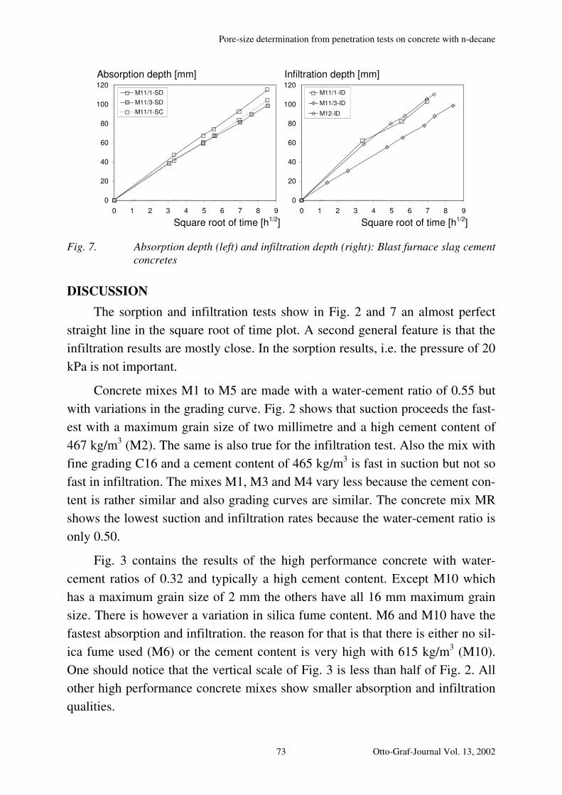
Pore-size determination from penetration tests on concrete with n-decane
0
20
40
60
80
100
120
0 1 2 3 4 5 6 7 8
Square root of time [h1
9/2]
M11/1-SD
M11/3-SD
M11/1-SC
Absorption depth [mm]
0
20
40
60
80
100
120
0 1 2 3 4 5 6 7 8 9
Square root of time [h1/2]
M11/1-ID
M11/3-ID
M12-ID
Infiltration depth [mm]
Fig. 7. Absorption depth (left) and infiltration depth (right): Blast furnace slag cement concretes
DISCUSSION
The sorption and infiltration tests show in Fig. 2 and 7 an almost perfect
straight line in the square root of time plot. A second general feature is that the
infiltration results are mostly close. In the sorption results, i.e. the pressure of 20
kPa is not important.
Concrete mixes M1 to M5 are made with a water-cement ratio of 0.55 but
with variations in the grading curve. Fig. 2 shows that suction proceeds the fast-
est with a maximum grain size of two millimetre and a high cement content of
467 kg/m3 (M2). The same is also true for the infiltration test. Also the mix with
fine grading C16 and a cement content of 465 kg/m3 is fast in suction but not so
fast in infiltration. The mixes M1, M3 and M4 vary less because the cement con-
tent is rather similar and also grading curves are similar. The concrete mix MR
shows the lowest suction and infiltration rates because the water-cement ratio is
only 0.50.
Fig. 3 contains the results of the high performance concrete with water-
cement ratios of 0.32 and typically a high cement content. Except M10 which
has a maximum grain size of 2 mm the others have all 16 mm maximum grain
size. There is however a variation in silica fume content. M6 and M10 have the
fastest absorption and infiltration. the reason for that is that there is either no sil-
ica fume used (M6) or the cement content is very high with 615 kg/m3 (M10).
One should notice that the vertical scale of Fig. 3 is less than half of Fig. 2. All
other high performance concrete mixes show smaller absorption and infiltration
qualities.
Otto-Graf-Journal Vol. 13, 2002 73

H.W. REINHARDT, A. PFINGSTNER
A blast furnace slag cement has been used in the mixes of Fig. 4. The sorp-
tive tests led to results which were similar to those with Portland cement and a
water-cement ratio of 0.55 (Fig. 2). The infiltration tests on M12 which has a
maximum grain size of 2 mm is different from the others since the infiltration
rate is rather high. A similar result has been obtained in Fig. 2 with Portland ce-
ment.
The absorption depth and the infiltration depth are rather similar as can be
seen from Figs. 5 to 7. The absolute results of MR, M1 to M5 and M11 and M12
are almost the same i. e. the influence of the grading curve is not so strong as in
the case of the absorbed fluid volume. However, a closer look to the small varia-
tions reveals that the trends of grain size and cement content are the same as in
the case of absorbed volume.
Fig. 6 shows the smallest absorption and infiltration depth as has been ex-
pected since these concretes are high performance ones.
Table 4 contains the values of the sorptivity and the penetration coefficient.
The sorptivity is the quotient of absorbed volume per area divided by the square
root of time. The penetration coefficient gives the penetration depth divided by
the square root of time. Both quantities characterise physical properties of a ma-
terial. Both material constants have been derived from sorption and infiltration
tests, So and Sp and Bo and Bp respectively.
The sorptivity So is in the range of 1.0 to 1.49 l m-2 h-1/2 for concrete with a
water-cement ratio of 0.55. The corresponding value Sp lies in the range of 1.11
to 1.97 l m-2 h-1/2. The difference between sorption test and infiltration test is
consistent. High performance concretes M6 to M10 show considerably lower
values So between 0.38 and 0.66 l m-2 h-1/2 and Sp between 0.47 and 0.76 l m-2
h-1/2 . The mixes with blast furnace slag cement fit into the ranges of mixes with
Portland cement except M12 in the infiltration test with a high value of 2.24 l
m-2 h-1/2.
The penetration coefficient Bo ranges between 12.2 and 14.1 mm h-1/2 for
mixes with a water-cement ratio of 0.55. Bp lies between 13.7 and 15.2 mm h-1/2,
i. e. a slight increase due to the pressure of 20 kPa. With a lower water-cement
ratio of 0.32 the Bo drops to 7.2 and 10.3 mm h-1/2 and Bp drops to 8.0 and 11.0
mm h-1/2. All results are consistent as the influence of grain size, water-cement
ratio and pressure are concerned. The B-values for blast furnace slag cement
concrete are similar to those of Portland cement concrete.
74

Pore-size determination from penetration tests on concrete with n-decane
The effective pore radius r can be calculated from Bo and Bp as shown in
Eq. (4) or equivalently also from the sorptivities since penetration coefficient
and sorptivity are linked together via the porosity ε (see Eq. (5)). Since the po-
rosity levels out a similar equation occurs for the sorptivity as for the penetration
coefficient.
Table 4 contains the results. It can be seen that the pore sizes range be-
tween about 0.2 to more than 1.0 µm when the content angle is taken to zero.
The values decrease when the cosine of the contact angle is taken as 2/π [3]. The
absorbed values increase with the water-cement ratio. A deviation is obvious for
M12 with blast furnace slag cement and a high cement content.
The values of r calculated from the sorptivity are always larger than calcu-
lated from the penetration coefficient. This feature is certainly due to the fact
that the single size tube model is only a rough approximation of reality. It reality
the smallest pores have the greatest capillary suction form while the complete
filling of the pores are lacking behind. This means that the penetration coeffi-
cient should take into account smaller pores than the sorptivity does.
As the absolute values of r are concerned these are rather large compared to
pore sizes which are calculated from many intrusion experiments [8]. Obviously,
the pores which are reached by the organic fluid are the larger ones and the very
small pores are either filled by water of are inaccessible due to other reasons, for
instance due to the viscosity of the fluid or of the size of the molecule. This
could also mean that the model of the sharp wetting front is questionable. On the
other hand, it means that the selection of various fluids could give an impression
of the pore sizes which can be detected.
CONCLUSIONS
∗ The experiments with n-decane have proven the capillary suction law which
states that the absorbed volume and the penetration depth are a function of
the square root of time.
∗ The water-cement ratio is the main parameter governing the absorption
properties.
∗ The infiltration test with 20 kPa leads only to a minor increase of the pene-
tration and absorption.
Otto-Graf-Journal Vol. 13, 2002 75
H.W. REINHARDT, A. PFINGSTNER
∗ The pore sizes determined from the absorption test are larger than from the
penetration test indicating a different access to pores by different mecha-
nisms.
∗ Maximum aggregate size and various cement contents lead to different
physical properties.
REFERENCES
[1] Reinhardt, H. W. (ed.): Penetration and permeability of concrete: barriers
to organic and contaminating liquids. London: E&FN Spon, 1997
[2] Aufrecht, M.: Beton als sekundäre Dichtbarriere gegenüber umweltgefähr-
denden Flüssigkeiten - Technologie und Konzept für den Schadensfall,
Dissertation Universität Stuttgart, 1994
[3] Sosoro, M.: Modell zur Vorhersage des Eindringverhaltens von organi-
schen Flüssigkeiten in Beton, DAfStb, H. 446, Berlin 1995
[4] Brauer, N.: Analyse der Transportmechanismen für wassergefährdende
Flüssigkeiten in Beton zur Berechnung des Medientransports in ungerisse-
ne und gerissene Betondruckzonen, DAfStb, H. 524, Berlin 2002
[5] Paschmann, H., Grube, H., Thielen, G.: Untersuchungen zum Eindringen
von Flüssigkeiten in Beton sowie zur Verbesserung der Dichtheit des Be-
tons. DAfStb, H. 450, Berlin 1995
[6] DAfStb Guideline "Betonbau beim Umgang mit wassergefährdenden Stof-
fen", Part 4, Berlin 1996
[7] Pfingstner, A.: Determination of concrete pore structure parameters from
penetration tests with n-decane, Otto Graf Journal 10 (1999), pp. 113-127
[8] Reinhardt, H.-W., Gaber, K.: From pore size distribution to an equivalent
pore size of cement mortar. In: Materials & Structures 23 (1990), pp. 3-15
76

Analysis of crystalline materials contained in a palestine kohl vessel from the 4th century A.D.
ANALYSIS OF CRYSTALLINE MATERIALS PRESERVED IN A PAL-ESTINE KOHL VESSEL FROM THE 4TH CENTURY A.D.
UNTERSUCHUNGEN AM KRISTALLINEN INHALT EINES KA-JALGLASES AUS PALÄSTINA, 4. JH. A.D.
ANALYSE DU CONTENU CRISTALLIN D'UN RECIPIENT A KHOL DE PALESTINE DATANT DU 4ÈME SIÈCLE A.D.
Friedrich Grüner
SUMMARY
The crystalline content of a Late Roman glass vessel used to hold cosmetic
eye shadow (kohl) was analysed. The analytical techniques used were X-ray
powder diffraction and scanning electron microscopy. The materials detected are
described, indicating that they may have been used as kohl.
ZUSAMMENFASSUNG
Es wurde der kristalline Inhalt eines spätrömischen Doppelglasgefäßes aus
Palästina mit Röntgenpulverdiffraktometrie und am Rastelektronenmikroskop
untersucht. Der Gefäßinhalt wurde wahrscheinlich als Augenschminke (Kajal)
benutzt.
RESUME
Le contenu cristallin d'un récipient romain provenant de Palestine a été ana-
lysé au diffractomètre poudre aux rayons X et au microscope électronique à ba-
layage. Le contenu du récipient était probablement utilisé comme maquillage
pour les yeux (khôl).
KEYWORDS: kohl, glass vessel, galena, anglesite, cerussite, x – ray diffraction
1. INTRODUCTION
The following is a report on a study of the materials contained in a double –
tube flask from the collection of the “Württembergisches Landesmuseum” in
Stuttgart. A typical glass vessel for holding cosmetic eye – paints might have
one, two or four individual tubes.
Otto-Graf-Journal Vol. 13, 2002 77
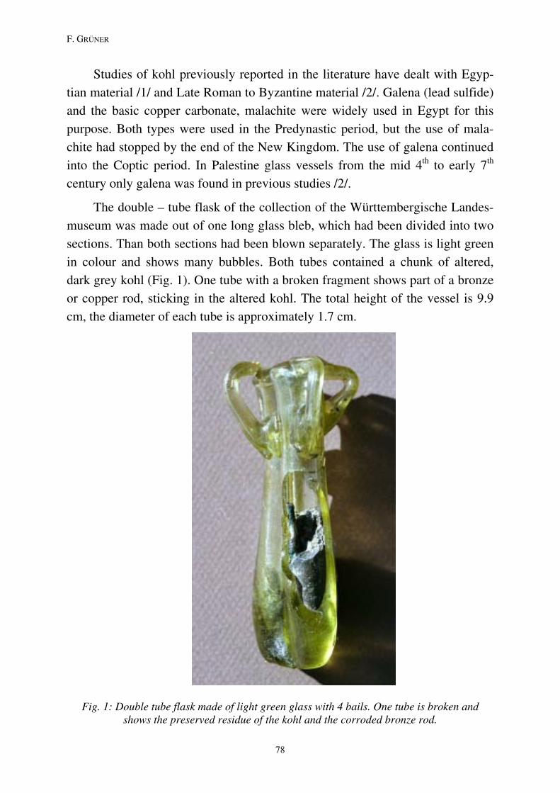
F. GRÜNER
Studies of kohl previously reported in the literature have dealt with Egyp-
tian material /1/ and Late Roman to Byzantine material /2/. Galena (lead sulfide)
and the basic copper carbonate, malachite were widely used in Egypt for this
purpose. Both types were used in the Predynastic period, but the use of mala-
chite had stopped by the end of the New Kingdom. The use of galena continued
into the Coptic period. In Palestine glass vessels from the mid 4th to early 7th
century only galena was found in previous studies /2/.
The double – tube flask of the collection of the Württembergische Landes-
museum was made out of one long glass bleb, which had been divided into two
sections. Than both sections had been blown separately. The glass is light green
in colour and shows many bubbles. Both tubes contained a chunk of altered,
dark grey kohl (Fig. 1). One tube with a broken fragment shows part of a bronze
or copper rod, sticking in the altered kohl. The total height of the vessel is 9.9
cm, the diameter of each tube is approximately 1.7 cm.
Fig. 1: Double tube flask made of light green glass with 4 bails. One tube is broken and shows the preserved residue of the kohl and the corroded bronze rod.
78
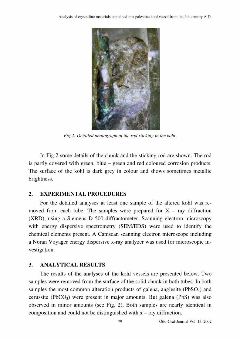
Analysis of crystalline materials contained in a palestine kohl vessel from the 4th century A.D.
Fig 2: Detailed photograph of the rod sticking in the kohl.
In Fig 2 some details of the chunk and the sticking rod are shown. The rod
is partly covered with green, blue – green and red coloured corrosion products.
The surface of the kohl is dark grey in colour and shows sometimes metallic
brightness.
2. EXPERIMENTAL PROCEDURES
For the detailed analyses at least one sample of the altered kohl was re-
moved from each tube. The samples were prepared for X – ray diffraction
(XRD), using a Siemens D 500 diffractometer. Scanning electron microscopy
with energy dispersive spectrometry (SEM/EDS) were used to identify the
chemical elements present. A Camscan scanning electron microscope including
a Noran Voyager energy dispersive x-ray analyzer was used for microscopic in-
vestigation.
3. ANALYTICAL RESULTS
The results of the analyses of the kohl vessels are presented below. Two
samples were removed from the surface of the solid chunk in both tubes. In both
samples the most common alteration products of galena, anglesite (PbSO4) and
cerussite (PbCO3) were present in major amounts. But galena (PbS) was also
observed in minor amounts (see Fig. 2). Both samples are nearly identical in
composition and could not be distinguished with x – ray diffraction.
Otto-Graf-Journal Vol. 13, 2002 79

F. GRÜNER
47-1734 (*) - Cerussite, syn - PbCO3 - Y: 10.30 % - d x by: 1. - WL: 1.5406 - Orthorho
05-0592 (I) - Galena, syn - PbS - Y: 14.79 % - d x by: 1. - WL: 1.5406 - Cubic - a 5.936
36-1461 (*) - Anglesite, syn - PbSO4 - Y: 75.98 % - d x by: 1. - WL: 1.5406 - Orthorho
83-1720 (C) - Anglesite - Pb(SO4) - Y: 69.31 % - d x by: 1. - WL: 1.5406 - Orthorhombi
SchminkeP2 - File: SchminkeP2.RAW - Type: 2Th/Th locked - Start: 5.000 ° - End: 70.
Sqr (Counts)
0
1
10
100
200
300
400
500
600
700
800
2-Theta - Scale
5 10 20 30 40 50 60 70
Fig. 2: XRD plot of the powdered kohl sample. Anglesite and cerussite occurred as common
alteration products, but galena is also present.
It is reasonable that finely ground galena for use as kohl would have
enough time to alterate into anglesite and cerrusite during ca. 1500 years of stor-
age under unknown archaeological conditions. The analyses of a small piece of
the rod, sticking inside the kohl showed cuprite and brochantite (see Fig. 3).
47-1734 (*) - Cerussite, syn - PbCO3 - Y: 0.61 % - d x by: 1. - WL: 1.5406 - Orthorhom
36-1461 (*) - Anglesite, syn - PbSO4 - Y: 8.38 % - d x by: 1. - WL: 1.5406 - Orthorhom
83-1720 (C) - Anglesite - Pb(SO4) - Y: 3.25 % - d x by: 1. - WL: 1.5406 - Orthorhombic
43-1458 (I) - Brochantite-M - Cu4SO4(OH)6 - Y: 2.72 % - d x by: 1. - WL: 1.5406 - Mon
75-1531 (C) - Cuprite - Cu2O - Y: 90.16 % - d x by: 1. - WL: 1.5406 - Cubic - a 4.26000
Schminke P1 - File: SchminkeP1.RAW - Type: 2Th/Th locked - Start: 5.000 ° - End: 70
Sqr (Counts)
0
10
100
1000
200
300
400
500
600
2000
3000
2-Theta - Scale
5 10 20 30 40 50 60 70
Fig. 3: XRD plot of a mixed sample with kohl (anglesite, cerussite) and alteration products of
the bronze rod (cuprite, brochantite).
80

Analysis of crystalline materials contained in a palestine kohl vessel from the 4th century A.D.
The complete vessel was placed under the scanning electron microscope
for further investigations. The original surface of the kohl was studied in the
broken tube. Elemental analysis showed high concentrations of lead and sulphur
and some copper in the surrounding material of the rod, indicating a bronze al-
loy or copper metal. Other elements like Sb were absent, eliminating the use of
stibnite as possible component in the kohl material.
Fig. 4: Elemental analysis of a galena cube at the surface showing mainly Pb,
S is buried by the Pb peak.
Photomicrographs of the surface are shown in Fig. 5 and 6. The kohl con-
sists of a very fine grained groundmass with hypidiomorphic intergrown cubes
of galena.
Fig. 5: Photomicrograph of the fine grained groundmass with intergrown galena cubes.
Otto-Graf-Journal Vol. 13, 2002 81

F. GRÜNER
Fig. 6: Detailed photomicrograph of a galena cube.
4. CONCLUSIONS
In this study evidence was found only for galena as material used for the
production of kohl. Both flasks contained identical materials. For its use as an-
cient make up (eye shadow) it should be ground very fine. It is reasonable to
assume that most of the galena is altered to anglesite and cerussite during the
long period of storage under unknown archaeological conditions.
5. ACKNOWLEDGEMENT
The author wish to thank Mrs. Dr. Honroth at the Württembergisches Lan-
desmuseum for providing the sample material.
REFERENCES
[1] LUCAS, A., 1962: Ancient Egyptian Materials and Industries, 4th ed., revised
by J.R. Harris (Edward Arnold, London, 1962), pp 80-84
[2] BLANCHARD, W.D., STERN, E.M., STODULSKI, L.P., 1992: Analysis of Mate-
rials contained in Mid-4th to Early 7th Century A.D. Palestinian Kohl Tubes,
Mat. Res. Soc. Symp. Proc. Vol. 267, pp 239-254
82

Acoustic emission analysis of SFRC beams under cyclic bending loads
ACOUSTIC EMISSION ANALYSIS OF SFRC BEAMS UNDER CYCLIC BENDING LOADS
SCHALLEMISSIONSANALYSE AN STAHLFASERBETON UNTER ZYKLISCHEN BIEGEVERSUCHEN
ANALYSE DES ÉMISSIONS ACOUSTIQUES DE BETONS RENFORCES PAR FIBRES D'ACIER SOUS FLEXION CYCLIQUE
Florian Finck
SUMMARY
To further understand the failure processes within steel fibre reinforced
concrete members under cyclic load, a series of 3-point bending tests was
performed on notched beams using quantitative acoustic emission (AE)
measurements. AE measurements supplement the mechanical test data by
providing a large quantity of information about the progress of damage in terms
of time, location and cause. Quantitative analysis of acoustic signals consists of
an accurate localization of the fracturing and under certain assumptions an
inversion for the moment tensor can be performed to gain information about the
total energy released and the orientation of the rupture plane. After
decomposition of the moment tensor, the type of rupture process can be
quantified and visualized using ostensive crack models like those for shear and
opening. In this article some first results of the fatigue test series and the
analysis of the AE-data are presented.
ZUSAMMENFASSUNG
Zur Untersuchung von Schädigungsprozessen innerhalb
stahlfaserbewehrter Betonbauteile unter zyklischer Last wurde eine Reihe von
3-Punkt-Biegeversuchen durchgeführt und die auftretenden Schallereignisse
aufgezeichnet. Neben den mechanischen Prüfdaten können so Informationen
über den Zeitpunkt und den genauen Ort der fortlaufenden Schädigung
gewonnen werden. Darüber hinaus kann unter bestimmten Voraussetzungen
eine Inversion auf den Momententensor durchgeführt werden, welcher
bruchmechanische Parameter, wie z. B. die Bruchenergie und die Orientierung
der Bruchflächen enthält. Nach einer geeigneten Zerlegung des Tensors können
die enthaltenen Bruchmoden quantifiziert und durch anschaulich Bruchmodelle,
Otto-Graf-Journal Vol. 13, 2002 83
F. FINCK
wie die des Öffnungs- oder des Scherbruches beschrieben werden. In diesem
Artikel werden erste Ergebnisse der Ermüdungsversuche und der
Schallemissionsanalyse vorgestellt.
RESUME
Afin d'analyser les processus de détérioration à l'intérieur d'éléments en
béton armé de fibres d'acier sous chargement cyclique, nous avons réalisé une
série d'essais de flexion 3 points et enregistré les émissions acoustiques. Ainsi
nous avons pu gagner, outre les données mécaniques, des informations sur la
nature, le moment et le lieu exacts des émissions acoustiques, et, par là, sur la
progression de la rupture. Dans certaines conditions, le tenseur des moments
peut être calculé par inversion. Celui-ci contient des informations sur l'énergie
libérée et l'orientation de la surface de rupture. Après la décomposition du
tenseur de moment, les modes de rupture peuvent être quantifiés et visualisés à
l'aide de modèles simples, comme ceux pour le cisaillement et l'ouverture. Dans
cet article les premiers résultats des essais de fatigue et de l'analyse des
émissions acoustiques sont présentés.
KEYWORDS: fatigue test, steel fibre reinforced concrete, acoustic emission,
moment tensor
INTRODUCTION
Steel fibre reinforced concrete (SFRC) has been in use since the late 60s,
mainly as shotcrete for underground constructions and flooring. Some
advantages of SFRC are a minimization of crack widths and permeability or an
increased toughness. Although various basic works on the behaviour of SFRC
members have been published [e.g. WEILER 2000], there remain open questions
about the mechanical laws and processes that exist during failure. The
interaction between steel fibre reinforcement and a cementitious matrix, as well
as the characterization of failure of SFRC members, are mayor topics of the
subproject A6 in the collaborative research centre SFB 381.
In a fatigue test series with steel fibre reinforced concrete (SFRC) beams
under cyclic 3-point bending load we studied the behaviour of ongoing failure.
Thereby, the investigation of acoustic emissions under changing conditions
(e. g. load, amplitude and frequency) was the main focus, not an accurate
statistical investigation of the members. The external, i. e. visible, fatigue is
84
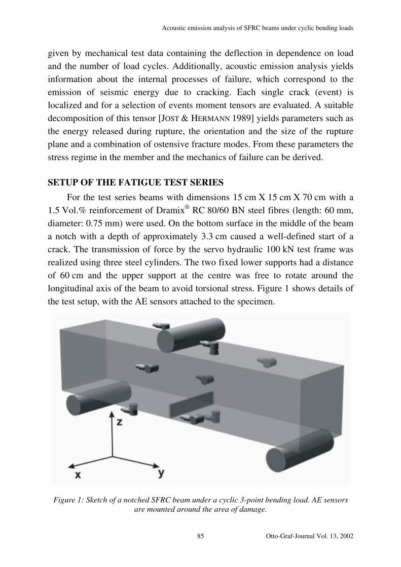
Acoustic emission analysis of SFRC beams under cyclic bending loads
given by mechanical test data containing the deflection in dependence on load
and the number of load cycles. Additionally, acoustic emission analysis yields
information about the internal processes of failure, which correspond to the
emission of seismic energy due to cracking. Each single crack (event) is
localized and for a selection of events moment tensors are evaluated. A suitable
decomposition of this tensor [JOST & HERMANN 1989] yields parameters such as
the energy released during rupture, the orientation and the size of the rupture
plane and a combination of ostensive fracture modes. From these parameters the
stress regime in the member and the mechanics of failure can be derived.
SETUP OF THE FATIGUE TEST SERIES
For the test series beams with dimensions 15 cm X 15 cm X 70 cm with a
1.5 Vol.% reinforcement of Dramix® RC 80/60 BN steel fibres (length: 60 mm,
diameter: 0.75 mm) were used. On the bottom surface in the middle of the beam
a notch with a depth of approximately 3.3 cm caused a well-defined start of a
crack. The transmission of force by the servo hydraulic 100 kN test frame was
realized using three steel cylinders. The two fixed lower supports had a distance
of 60 cm and the upper support at the centre was free to rotate around the
longitudinal axis of the beam to avoid torsional stress. Figure 1 shows details of
the test setup, with the AE sensors attached to the specimen.
Figure 1: Sketch of a notched SFRC beam under a cyclic 3-point bending load. AE sensors are mounted around the area of damage.
Otto-Graf-Journal Vol. 13, 2002 85
F. FINCK
Piston displacement, load and crack opening were recorded over time. The
acoustic emissions were recorded by an 8-channel transient recorder with a
sample rate of 2.5 MHz per channel and an amplitude resolution of 12 Bit. Eight
piezo-electric accelerometers were evenly distributed on the surfaces of the
beam.
First, the range of the failure load was evaluated in two static bending tests.
Although, a large variation of this value has to be expected due to a change in
the distribution of fibres and the composition of concrete in the beam, this value
provides an estimate of the load profile for the dynamic tests. During the
dynamic tests, load, amplitude and frequency were adapted to the progress of
damage and the AE activity.
PRESENTATION OF THE RESULTS
In the following section the results of one test run are presented. A load of
7.5 kN was applied statically before the load cycles began. In the second plot in
figure 2 the different phases with changing load, amplitude and frequency
during the fatigue test are labelled and coded by blue (dark grey) and green
(light grey) respectively to be identified in the load over crack opening
(displacement) plot and the crack opening over time or cycles plot. The
frequency of the sinusoidal load cycles was 1 Hz from phase G. From that point
the number of load cycles equals time in seconds plus 5000. On the bottom a
histogram of the acoustic emission activity can be correlated with the ongoing
failure in the beam.
With each increase of the maximum load the crack opening, as well as the
AE activity, increases rapidly but a relaxation is visible with the continuation of
the test. The extending areas of the hysteretic ellipses in the load over crack
opening plots are another indicator for the damage progress.
86

Acoustic emission analysis of SFRC beams under cyclic bending loads
Figure 2: Mechanical test data of one fatigue test. From top: load deflection curve,
load over time profile, crack opening over time and the AE activity.
Otto-Graf-Journal Vol. 13, 2002 87
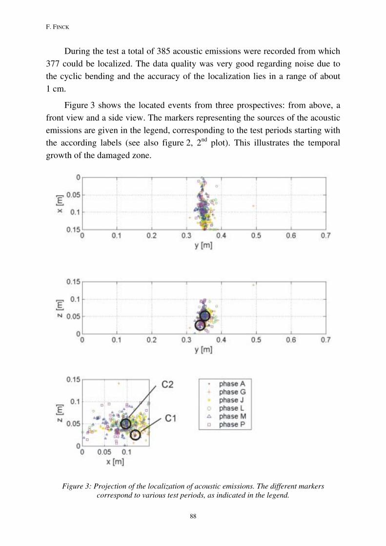
F. FINCK
During the test a total of 385 acoustic emissions were recorded from which
377 could be localized. The data quality was very good regarding noise due to
the cyclic bending and the accuracy of the localization lies in a range of about
1 cm.
Figure 3 shows the located events from three prospectives: from above, a
front view and a side view. The markers representing the sources of the acoustic
emissions are given in the legend, corresponding to the test periods starting with
the according labels (see also figure 2, 2nd plot). This illustrates the temporal
growth of the damaged zone.
Figure 3: Projection of the localization of acoustic emissions. The different markers correspond to various test periods, as indicated in the legend.
88

Acoustic emission analysis of SFRC beams under cyclic bending loads
Nearly all acoustic emissions lie in the central region of the specimen in the
vicinity of the main crack. Due to the steel fibres, some smearing of the damage
zone takes place. The early events come from the lower half of the specimen
since the crack starts in the edge of the notch due to tension. Then steel fibres
are activated and accommodate load as they are pulled out. The crack grows
towards the top of the specimen under a relative constant spatial AE activity
from the complete region under fatigue. The width of the damage zone in y-
direction is more or less in the range of the fibre length (i. e. 60 mm). This
suggests that always the short end of the fibre is being pulled out, as expected.
THE INVERSION OF MOMENT TENSORS
To gather more information about the mechanical reasons of failure, we
calculate moment tensors with a relative moment tensor inversion (RMTI)
technique developed by DAHM 1993. The application and some theory of this
method on acoustic emission data has been described previously [e. g. FINCK
2002, FINCK 2001, GROSSE 1999]. An advantage of the RMTI is the elimination
of the Green’s functions [AKI & RICHARDS 1980] of the medium by an inversion
for a cluster of events. Two circles in figure 3 indicate the orientation of two
clusters of 16 events each which were inverted for their moment tensors. C1 is a
cluster from very early events in the tension zone, events in C2 originate from
an advanced stage of the test.
Figure 4: Radiation patterns of seismic energy and results from the moment tensor inversion for selected events from cluster C1 an C2 (see figure 3). Mr is the relative seismic moment,
ISO is the isotropic component of the event and DC is the double-couple portion of the deviatoric component.
Otto-Graf-Journal Vol. 13, 2002 89

F. FINCK
A combination of two different crack modes is expected for the performed
test. First, the opening of the main crack should radiate energy similar to event
EV 29 in cluster C1. An opening mainly perpendicular to the vertical crack-
surface with particle motion outwards parallel to the y-axis and a significant
remaining isotropic component. This conforms to mode 1. Second, a great
number of events should correspond to the pull-out of steel fibres. Mainly a
double couple mechanism for shear failure is expected in this case, with a small
isotropic component only (conforming mode 2 or 3).
A selection of the results is shown in figure 4. The first row contains results
for cluster C1, the second for C2. Under the top view projection of the radiation
patterns of seismic energy the relative seismic moment Mr, the isotropic
component ISO and the double-couple portion DC of the deviatoric component
are given with errors. The best results from a boot strap analysis [EFRON &
TIBSHIRANI, 1986] can be found in the brackets. The majority of the moment
tensors consist of a very small positive isotropic component. For event EV 29
the errors are very high, so the results must be doubted, though the radiation
pattern fits to first expectations. For the other events in C1 the DC component is
rather small. The deviatoric components of these events can not be explained by
one pure shear crack. Other deviatoric phenomena seem to take place. But the
early events in C1 vary from the results for C2. The events occurred at an
advanced stage of the test, where the fibre-pull out seems to be the major reason
for acoustic activity. Here, the DC component is large.
The results have a great stability for a changing composition of the
investigated clusters. In earlier investigations the results for single events were
dependent on the composure of the cluster, meaning that the existence or non-
existence of other events had an influence on the results. Also the errors are
small.
CONCLUSIONS
We successfully obtained high quality acoustic emission data from cyclic
bending tests of steel fibre reinforced concrete beams. The majority of these
events could be localized and an inversion for the moment tensor of a selection
of events was performed. Stable results from the moment tensor inversion can
partially be correlated with the expected mechanisms of failure – an opening of
the crack (mode 1) and mainly the pull-out of fibres (mode 2 or 3). Acoustic
90
Acoustic emission analysis of SFRC beams under cyclic bending loads
emission analysis helps understanding complex mechanisms of failure even over
a large period of time.
The decomposition of the moment tensor into crack modes known from
geological investigations seem not to be suitable for experimental data from the
laboratory. A decomposition taking crack modes from engineering models in to
account, is needed. This subject will be of intensive interest in future
ACKNOWLEDGEMENTS
These investigations are part of our work in the collaborative research
centre SFB 381 at the University of Stuttgart which is financially supported by
the Deutsche Forschungsgemeinschaft (DFG). We gratefully acknowledge this
support. The author would also like to thank Lindsay Linzer, Rock Engineering
Dept., CSIR Miningtek for providing the radiation pattern generator.
REFERENCES
AKI, K., RICHARDS, P.G.: Quantitative Seismology; Volume 1. Freeman and
Company, New York, 1980.
DAHM, T.: Relativmethoden zur Bestimmung der Abstrahlcharakteristik von
seismischen Quellen. Dissertation, Universität Karlsruhe, 1993.
EFRON, B. TIBSHIRANI, R.: Bootstrap methods for standard errors, confidence
intervals and other measures of statistical accuracy. Statistical Science 1,
pp.54-77, 1986.
FINCK, F.: Application of the moment tensor inversion in material testing. Otto-
Graf-Journal, Vol. 12, pp. 145-156, 2001.
FINCK, F., MOTZ, M., GROSSE, C.U., REINHARDT, H.-W., KRÖPLIN, B.:
Integrated Interpretation and Visualization of a Pull-Out Test using Finite
Element Modelling and Quantitative Acoustic Emission Analysis. Online
publication: http://www.ndt.net/article/v07n09/09/09.htm, 2002.
GROSSE, C.U.: Grundlagen der Inversion des Momententensors zur Analyse von
Schallemissionsquellen. Werkstoffe und Werkstoffprüfung im Bauwesen.
Festschrift zum 60. Geburtstag von Prof. Dr.-Ing. H.-W. Reinhardt, Libri
BOD, Hamburg, pp. 82-105, 1999.
Otto-Graf-Journal Vol. 13, 2002 91

F. FINCK
JOST, M.L., HERMANN, R.B.: A students guide to and review of moment tensors.
Seism. Res. Letters, Vol. 60, pp. 37-57, 1989.
WEILER, B.: Zerstörungsfreie Untersuchung von Stahlfaserbeton. Dissertation an
der Universität Stuttgart, Shaker Verlag, 2000.
92
About the Improvement of US measurement techniques
ABOUT THE IMPROVEMENT OF US MEASUREMENT TECHNIQUES FOR THE QUALITY CONTROL OF FRESH CONCRETE
GERÄTETECHNISCHE FORTSCHRITTE BEI DER QUALITÄTS-SICHERUNG VON FRISCHBETON MIT ULTRASCHALL
AMÉLIORATION DES TECHNIQUES DE MESURE ULTRASONIQUES POUR LE CONTRÔLE DE QUALITÉ DU BÉTON FRAIS.
Christian U. Grosse
ABSTRACT
Over the last decade a testing method based on ultrasound was developed
at the Institute of Construction Materials of the University of Stuttgart to control
the hardening process of cementitious materials by means of non-destructive
testing. This paper describes the systematic improvement and re-design of the
testing system and the investigation methods.
ÜBERSICHT
Am Institut für Werkstoffe im Bauwesen der Universität Stuttgart wurde in
den letzten zehn Jahren ein Ultraschallverfahren zur die Analyse des Erstarrens
und Erhärtens von zementgebundenen Materialien entwickelt. Der Artikel
beschreibt die fortdauernde Verbesserung der Messtechnik im Hinblick auf die
Qualitätskontrolle von Frischbeton und –mörtel.
RESUME
A l'université de Stuttgart, un procédé ultrasonique de contrôle de la prise
et du durcissement des matériaux cimentaires a été développé au courant des dix
dernières années. L'article présent décrit l'amélioration continue des dispositifs
et de la procédure de mesurage en ce qui concerne le contrôle de la qualité des
béton et mortiers frais.
KEYWORDS: Fresh concrete, non-destructive testing, ultrasound
Otto-Graf-Journal Vol. 13, 2002 93

C. U. GROSSE
INTRODUCTION
Nowadays the characterization of cement-based materials during the
stiffening process by ultrasound measurement techniques is well established.
This paper deals with the ultrasound technique used in through transmission. In
numerous publications [e. g. GROSSE & REINHARDT 1994, GROSSE ET AL. 1999,
REINHARDT ET AL. 1999a] the patented test method [REINHARDT ET AL. 1999b]
developed at the University of Stuttgart was described earlier. Methods based on
ultrasound are better suited for the characterization of the setting and hardening
of cement based materials than traditional test methods like the Vicat-needle-
test, the penetrometer test or the flow test, because the travel time, the
attenuation and the frequency content of ultrasound waves sent through the
material are closely correlated with the elastic properties of concrete or mortar.
These parameters can be continuously monitored during the stiffening giving a
comprehensive picture instead of snapshots of workability for example.
A sophisticated device was developed and numerous experiments have
been conducted in the past, investigating the influence of water-to-cement ratio,
the type of cement, the use of additives and admixtures, the air bubble content
and so far, for the setting and hardening of concrete or mortar. Newer features
are the extraction of the initial and final setting time out of the signals [GROSSE
& REINHARDT 2000] and the parallel registration of the state of hydration.
However, the earlier described device lacks of handiness and several features,
which could improve the art of such measurements further.
EVOLUTION AND SURVEY OF DEVICES EXISTING AT THE UNIVERSITY OF STUTTGART
The first measurements to control the setting and hardening of concrete at
the University of Stuttgart using ultrasound are dated back to the early 1990’s.
These experiments have been conducted in the frame of a research project
sponsored by the German Reinforced Concrete Committee (DAfStb, V 345) and
are published in the 1994th volume of the Otto-Graf-Journal [GROSSE &
REINHARDT 1994]. The tests were carried out with a rough set-up using a
container made of 40 mm thick styrene foam (Styropor) plates and the dimensions
300 mm × 300 mm × 80 mm (Fig. 1). The emitter was a simple steel ball impactor
dropping a ball of 4 mm diameter on to a small aluminium plate, which was placed
in contact with the fresh concrete.
94

About the Improvement of US measurement techniques
Fig. 1: Set-up with steel ball impactor and receiver. Dimensions of the container: 300 mm x 300 mm x 80 mm
Later on the ideas were proofed by numerous students during their Diploma
thesis, technician and student research assistants. Jochen FISCHER [1994], Bernd
Weiler and the author [Grosse 1996] developed a device using three long styrene
foam walls and two smaller rigid side walls out of aluminium plates and the same
simple impactor as used earlier (Fig. 2).
Fig. 2: Set-up of the smaller styrene foam container with two aluminium side walls. Dimensions of the container: 200 mm x 80 mm x 60 mm.
Otto-Graf-Journal Vol. 13, 2002 95

C. U. GROSSE
While the first set-up caused problems to determine the correct travel
distance of the pulse to the receiver, what is essential for velocity measurements,
the second set-up was unsatisfactory as well, because of interfering waves
resulting from the walls.
A re-design of the device described in REINHARDT ET AL. [1996], WINDISCH
[1996], HERB [1996] and REINHARDT ET AL. [1998] for concrete measurements
was patented later [Reinhardt et al. 1999] and consisted of a mould completely
out of PMMA of the dimensions 160 mm × 200 mm × 70 mm (Fig. 3), but the
handling of this device was poor and the leakiness of the container caused a
penetration of fluids especially during the compaction process. However, the
device was modified by BEUTEL [1999] and tested to be suitable for field
measurements.
Fig. 3: Set-up of the first container out of PMMA only. Dimensions of the container: 160 mm x 200 mm x 70 mm.
In the meantime the development of a test set-up adjusted to mortar
materials run parallel. Due to smaller grain sizes (usually less 2 mm) the
dimensions of a mortar device can significantly be reduced. Not all steps of the
development can be described in detail. Figure 4 gives an impression of the
iterative process of finding a suitable shape for the mould. The final container
[GROSSE ET AL. 1999] had two walls of PMMA and a U-shaped rubber foam
with an inner volume of 40 cm³ for the mortar (Fig. 5).
96
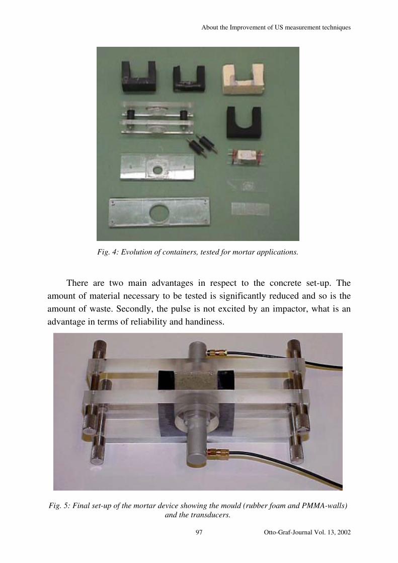
About the Improvement of US measurement techniques
Fig. 4: Evolution of containers, tested for mortar applications.
There are two main advantages in respect to the concrete set-up. The
amount of material necessary to be tested is significantly reduced and so is the
amount of waste. Secondly, the pulse is not excited by an impactor, what is an
advantage in terms of reliability and handiness.
Fig. 5: Final set-up of the mortar device showing the mould (rubber foam and PMMA-walls) and the transducers.
Otto-Graf-Journal Vol. 13, 2002 97
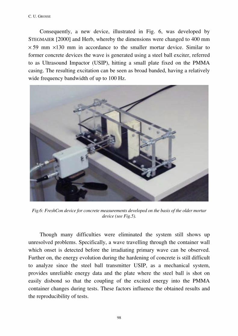
C. U. GROSSE
Consequently, a new device, illustrated in Fig. 6, was developed by
STEGMAIER [2000] and Herb, whereby the dimensions were changed to 400 mm
× 59 mm ×130 mm in accordance to the smaller mortar device. Similar to
former concrete devices the wave is generated using a steel ball exciter, referred
to as Ultrasound Impactor (USIP), hitting a small plate fixed on the PMMA
casing. The resulting excitation can be seen as broad banded, having a relatively
wide frequency bandwidth of up to 100 Hz.
Fig.6: FreshCon device for concrete measurements developed on the basis of the older mortar device (see Fig.5).
Though many difficulties were eliminated the system still shows up
unresolved problems. Specifically, a wave travelling through the container wall
which onset is detected before the irradiating primary wave can be observed.
Further on, the energy evolution during the hardening of concrete is still difficult
to analyze since the steel ball transmitter USIP, as a mechanical system,
provides unreliable energy data and the plate where the steel ball is shot on
easily disbond so that the coupling of the excited energy into the PMMA
container changes during tests. These factors influence the obtained results and
the reproducibility of tests.
98
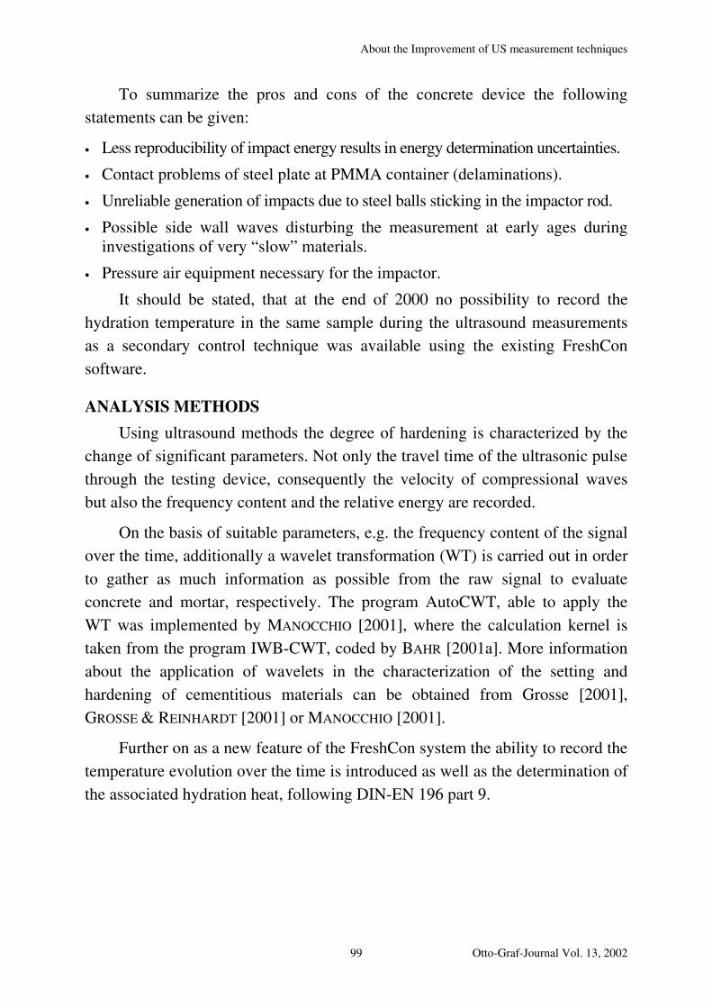
About the Improvement of US measurement techniques
To summarize the pros and cons of the concrete device the following
statements can be given:
• Less reproducibility of impact energy results in energy determination uncertainties.
• Contact problems of steel plate at PMMA container (delaminations).
• Unreliable generation of impacts due to steel balls sticking in the impactor rod.
• Possible side wall waves disturbing the measurement at early ages during investigations of very “slow” materials.
• Pressure air equipment necessary for the impactor.
It should be stated, that at the end of 2000 no possibility to record the
hydration temperature in the same sample during the ultrasound measurements
as a secondary control technique was available using the existing FreshCon
software.
ANALYSIS METHODS
Using ultrasound methods the degree of hardening is characterized by the
change of significant parameters. Not only the travel time of the ultrasonic pulse
through the testing device, consequently the velocity of compressional waves
but also the frequency content and the relative energy are recorded.
On the basis of suitable parameters, e.g. the frequency content of the signal
over the time, additionally a wavelet transformation (WT) is carried out in order
to gather as much information as possible from the raw signal to evaluate
concrete and mortar, respectively. The program AutoCWT, able to apply the
WT was implemented by MANOCCHIO [2001], where the calculation kernel is
taken from the program IWB-CWT, coded by BAHR [2001a]. More information
about the application of wavelets in the characterization of the setting and
hardening of cementitious materials can be obtained from Grosse [2001],
GROSSE & REINHARDT [2001] or MANOCCHIO [2001].
Further on as a new feature of the FreshCon system the ability to record the
temperature evolution over the time is introduced as well as the determination of
the associated hydration heat, following DIN-EN 196 part 9.
Otto-Graf-Journal Vol. 13, 2002 99

C. U. GROSSE
Fig. 7: Set-up (top) for measurements of elastic parameters (velocity, energy, frequency) as well as the temperatures. Bottom: Screenshot of the new program version 2.04 of FreshCon.
100
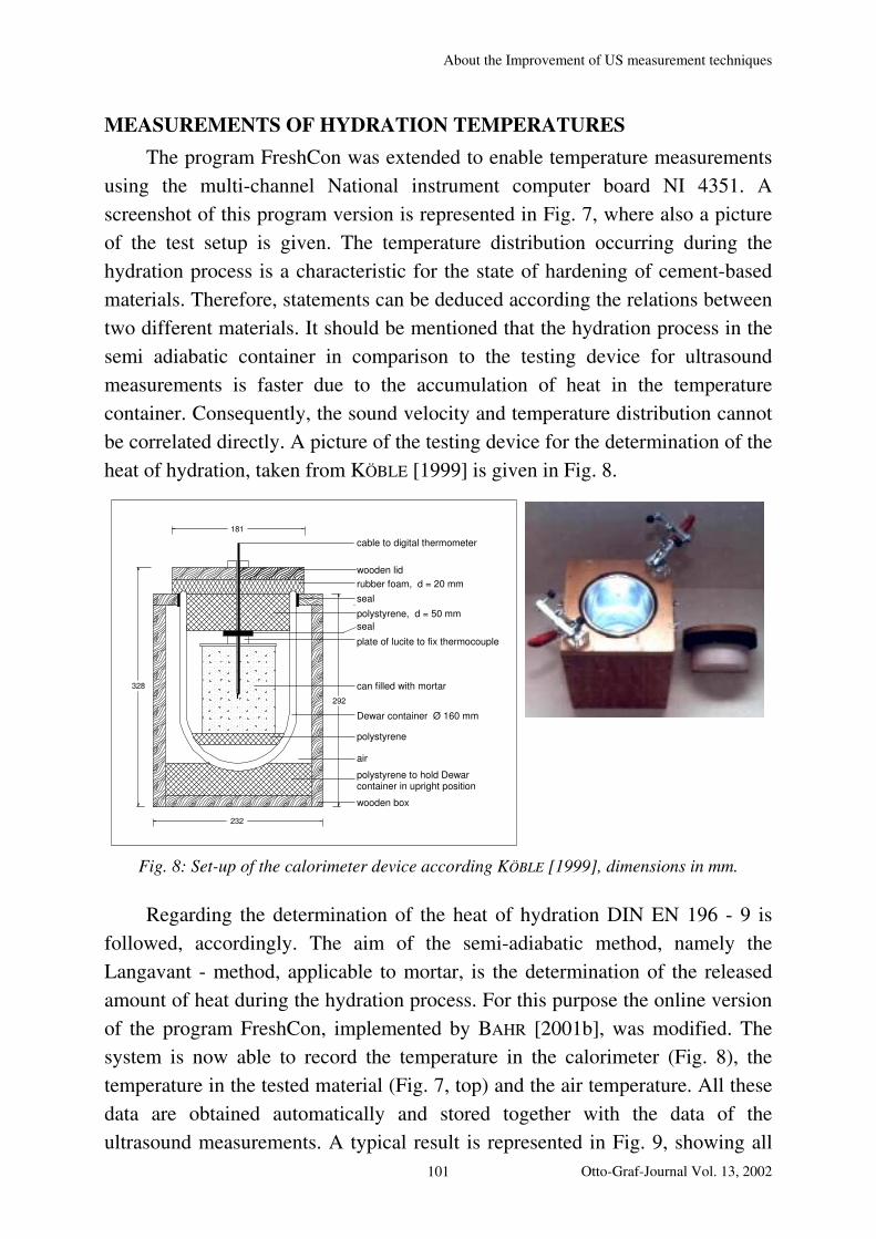
About the Improvement of US measurement techniques
MEASUREMENTS OF HYDRATION TEMPERATURES
The program FreshCon was extended to enable temperature measurements
using the multi-channel National instrument computer board NI 4351. A
screenshot of this program version is represented in Fig. 7, where also a picture
of the test setup is given. The temperature distribution occurring during the
hydration process is a characteristic for the state of hardening of cement-based
materials. Therefore, statements can be deduced according the relations between
two different materials. It should be mentioned that the hydration process in the
semi adiabatic container in comparison to the testing device for ultrasound
measurements is faster due to the accumulation of heat in the temperature
container. Consequently, the sound velocity and temperature distribution cannot
be correlated directly. A picture of the testing device for the determination of the
heat of hydration, taken from KÖBLE [1999] is given in Fig. 8.
Stützvorrichtung aus Polystyrol
Gehäuse aus Holz
Polystyrolscheibe
Mörteldose, h = 12cm
Dichtung
Polystyrol, d = 5cm
Zellgummidichtung, d = 2cm
Holzdeckel
Dewar-Gefäß
Plexiglasscheibe zum fixieren des Temperaturfühlers
16cm
Thermokabel geführt in einem Plexiglasröhrchen
Dichtung
181
292
232
328
Luft
cable to digital thermometer
wooden lid
wooden box
rubber foam, d = 20 mm
seal
seal
polystyrene, d = 50 mm
polystyrene
plate of lucite to fix thermocouple
can filled with mortar
Dewar container Ø 160 mm
polystyrene to hold Dewar container in upright position
air
Fig. 8: Set-up of the calorimeter device according KÖBLE [1999], dimensions in mm.
Regarding the determination of the heat of hydration DIN EN 196 - 9 is
followed, accordingly. The aim of the semi-adiabatic method, namely the
Langavant - method, applicable to mortar, is the determination of the released
amount of heat during the hydration process. For this purpose the online version
of the program FreshCon, implemented by BAHR [2001b], was modified. The
system is now able to record the temperature in the calorimeter (Fig. 8), the
temperature in the tested material (Fig. 7, top) and the air temperature. All these
data are obtained automatically and stored together with the data of the
ultrasound measurements. A typical result is represented in Fig. 9, showing all
Otto-Graf-Journal Vol. 13, 2002 101

C. U. GROSSE
three temperatures as a function of the concrete age. The temperature effect is
dominant at the curve obtained using the calorimeter (straight line) due to the
semi-adiabatic conditions in the Dewar container. Testing concrete materials a
hydration effect is clearly seen at the temperature data obtained in the ultrasound
container (dotted line) compared to the air temperature (dashed line).
0 200 400 600 800 1000 1200 1400
0
5
10
15
20
25
30
35
40
45
Rilem Round Robin TestsiBMB: 18/19 Apr 2002
Mixture: RB03 (concrete)
Remarks: very dry, water added
Hyd
ratio
n H
ea
t [°
C]
Concrete
Air
Air
an
d C
on
cre
te te
mp
era
ture
[°C
]
Time [min]
0
5
10
15
20
25
30
35
40
45
Hydration
Fig. 9: Results of temperature measurements using the new FreshCon version.
DEVELOPMENT OF A NEW CONCRETE FRESHCON DEVICE
Comparing the two devices for mortar and concrete measurements, the
advantages of the mortar set-up should be summarized:
• Good reproducibility of signal generation (energy).
• Easy onset time determination due to signals with good reproducibility.
• No pressure air equipment necessary.
• Full automatic measurement and storing of waveforms.
• Automatic determination of velocity and energy as well as additional parameters.
• Full control of measurement parameters.
To enhance the handling of concrete experiments accordingly, a new
design of the device shown in Fig. 6 was suggested. For the new device the
102

About the Improvement of US measurement techniques
impactor was replaced by an US transmitter in combination with a wideband
power amplifier and a function generator. No pressure air is need for this device;
a control sensor next to the impactor recording the emitting pulse is no longer
required.
0 120 240 360 480 600 7200
500
1000
1500
2000
velocity impactor
velocity piezo
rel. energy impactor
rel. energy piezo
age [min]velo
city [m
/s]
1E-6
1E-5
1E-4
1E-3
0.01
0.1
1
Fig. 10: Comparison experiments between impactor and US emitter.
rel. e
nerg
y [-]
In several preliminary experiments the new set-up was tested by
MANOCCHIO [2001] to compare the results of measurements by the impact
generated signals and by piezo-electric emitters in parallel (Fig. 10). The two
curves at the bottom of the right side in Fig. 10, recorded at the same time using
the same material, represent the velocity evaluation of gypsum. Gypsum was
used as a test material due to its fast hydration evolution. The two curves at the
top position in Fig. 10 represent the relative energy. A decrease of the velocity
and energies values is caused by shrinkage effects. Both curve pairs look very
similar in respect to differently used pulse generation methods.
This successful first test triggered the re-design of the concrete device (as
well as of the mortar device). A flow chart of the new experimental set-up is
given in Fig. 11. The electronic pulse is generated by a frequency generator and
amplified by a power amplifier. Broadband piezo-electric transducers generate
the ultrasound signal to be transmitted through the material. A transducer of the
same type is used as a receiver and the signal is passed through a pre-amplifier
to the PC-board A/D-converter, denoted as “computer-based signal processing”
in Fig. 11. Special attention is given to the correct trigger time of the signal,
what is essential for velocity measurements. A power amplifier of the companies
KROHN-HITE CO. or DEVELOGIC GMBH is used along with sensors of the
company VALLEN INSTRUMENTS.
Otto-Graf-Journal Vol. 13, 2002 103
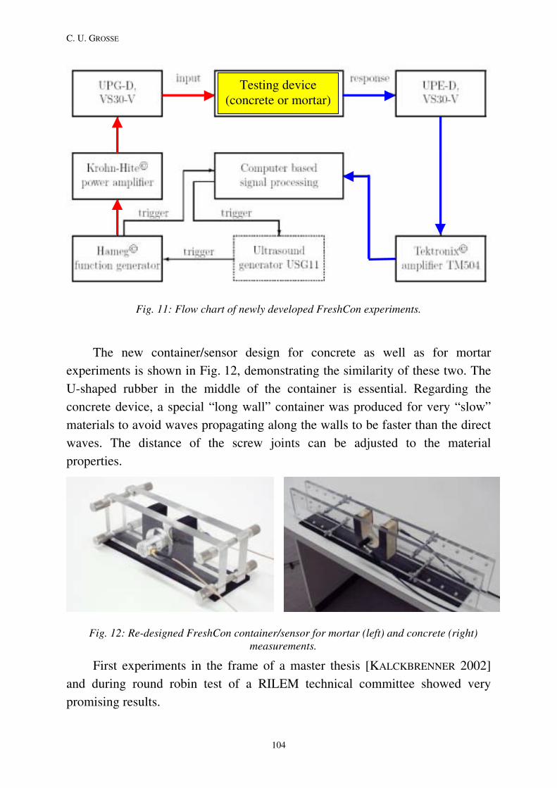
C. U. GROSSE
Fig. 11: Flow chart of newly developed FreshCon experiments.
Testing device (concrete or mortar)
The new container/sensor design for concrete as well as for mortar
experiments is shown in Fig. 12, demonstrating the similarity of these two. The
U-shaped rubber in the middle of the container is essential. Regarding the
concrete device, a special “long wall” container was produced for very “slow”
materials to avoid waves propagating along the walls to be faster than the direct
waves. The distance of the screw joints can be adjusted to the material
properties.
Fig. 12: Re-designed FreshCon container/sensor for mortar (left) and concrete (right) measurements.
First experiments in the frame of a master thesis [KALCKBRENNER 2002]
and during round robin test of a RILEM technical committee showed very
promising results.
104
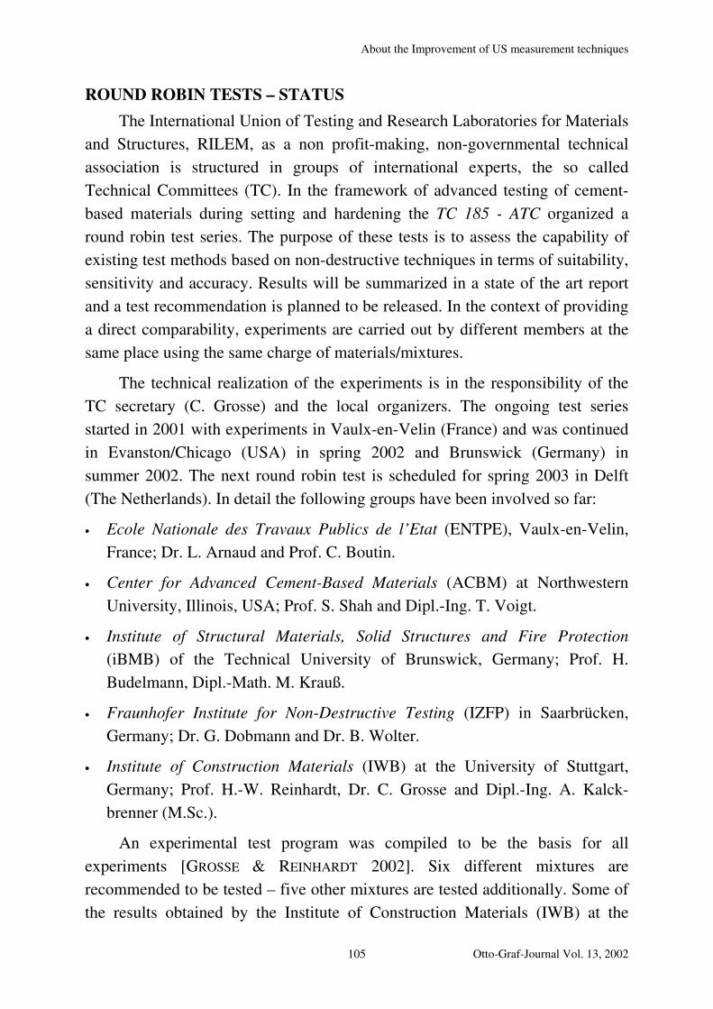
About the Improvement of US measurement techniques
ROUND ROBIN TESTS – STATUS
The International Union of Testing and Research Laboratories for Materials
and Structures, RILEM, as a non profit-making, non-governmental technical
association is structured in groups of international experts, the so called
Technical Committees (TC). In the framework of advanced testing of cement-
based materials during setting and hardening the TC 185 - ATC organized a
round robin test series. The purpose of these tests is to assess the capability of
existing test methods based on non-destructive techniques in terms of suitability,
sensitivity and accuracy. Results will be summarized in a state of the art report
and a test recommendation is planned to be released. In the context of providing
a direct comparability, experiments are carried out by different members at the
same place using the same charge of materials/mixtures.
The technical realization of the experiments is in the responsibility of the
TC secretary (C. Grosse) and the local organizers. The ongoing test series
started in 2001 with experiments in Vaulx-en-Velin (France) and was continued
in Evanston/Chicago (USA) in spring 2002 and Brunswick (Germany) in
summer 2002. The next round robin test is scheduled for spring 2003 in Delft
(The Netherlands). In detail the following groups have been involved so far:
• Ecole Nationale des Travaux Publics de l’Etat (ENTPE), Vaulx-en-Velin,
France; Dr. L. Arnaud and Prof. C. Boutin.
• Center for Advanced Cement-Based Materials (ACBM) at Northwestern
University, Illinois, USA; Prof. S. Shah and Dipl.-Ing. T. Voigt.
• Institute of Structural Materials, Solid Structures and Fire Protection
(iBMB) of the Technical University of Brunswick, Germany; Prof. H.
Budelmann, Dipl.-Math. M. Krauß.
• Fraunhofer Institute for Non-Destructive Testing (IZFP) in Saarbrücken,
Germany; Dr. G. Dobmann and Dr. B. Wolter.
• Institute of Construction Materials (IWB) at the University of Stuttgart,
Germany; Prof. H.-W. Reinhardt, Dr. C. Grosse and Dipl.-Ing. A. Kalck-
brenner (M.Sc.).
An experimental test program was compiled to be the basis for all
experiments [GROSSE & REINHARDT 2002]. Six different mixtures are
recommended to be tested – five other mixtures are tested additionally. Some of
the results obtained by the Institute of Construction Materials (IWB) at the
Otto-Graf-Journal Vol. 13, 2002 105

C. U. GROSSE
University of Stuttgart are published by KALCKBRENNER [2002] and correlated
to the results of other groups. A comprehensive report will follow.
To give an example of the data obtained during one test series Fig. 13
demonstrate the variation of the velocities over the age of the material.
Concerning these velocities an S-shaped curve is typical for cementitious
materials. After a certain time at the beginning, while the velocity variation is
small, the gradient is increasing significantly. Regarding the data RE5 from a
mix with added retarder this increase occurs relatively late. To make the basic
statements more evident the curves are smoothed and bad data points are
removed. It is obvious that concrete mixes are “faster” than mortar mixes in
respect to hardening, while the RE5 mix with retarder is the “slowest“ material.
Fig. 13: Comparison of the velocity measurements testing mixtures RE 1-6.
0 200 400 600 800 1000 1200 1400
0
1000
2000
3000
4000
5000
Ve
locity [m
/s]
Age [min]
RE1: concrete, w.c. 0.45
RE2: concrete, w.c. 0.60
RE3: mortar, w.c. 0.60
RE4: mortar, with plasticizer
RE5: mortar, with retarder
RE6: mortar, with air entrainer
smoothed!
It should be stressed that only material properties related to the elastic behavior
can be analyzed with ultrasound techniques. As far as the chemical properties
are not related to the elastic properties, other measurement techniques have to be
used in combination with ultrasound to get more data. The results of the round
robin tests should indicate the value of the described ultrasound through-
transmission technique in comparison to other techniques like ultrasound
reflection, nuclear magnetic resonance, electric and maturity methods.
106
About the Improvement of US measurement techniques
SUMMARY AND OUTLOOK
The measuring device developed at the University of Stuttgart is able to
analyze the setting and hardening of cementitious materials in a comprehensive
way. The method is based on ultrasound and can be used for numerous
applications, where reliable and reproducible data are required, what addresses
material parameters like the water-to-cement-ratio, the type of cement or the
effect of additives as retarders or accelerators. At the concreting site, where
efficiency and a low budget are boundary conditions, the application of this new
technique can help to enhance the stability during construction or the progress of
the construction work saving both: time and money. Some examples are the
development of admixtures, the in-situ quality control, the slip form concreting
or the precasting. Certainly, the applications are not restricted to cementitious
materials.
Further improvements are concerning the velocity evaluation. Since the
device consist of an analogue-to-digital converter of 5 MHz only, the resolution
of the velocity calculations varies over age. Actually, the resolution decreases
with increasing velocities. This is the reason of the so-called bit-pattern
occurring usually at ages of 400 minutes and later. To ease the interpretation the
velocity curves are smoothed using adjacent averaging (10 points), but it is
suggested to plot the original data points into the smoothed curves as well.
Using the offline version of the FreshCon picking algorithm the data can be re-
evaluated after the test concerning the onset times of the signals only.
Surprisingly, curves re-picked by the operator are usually very similar to the
automatically processed data so that a time consuming manually picking is not
improving the results anymore.
Formerly, the comparison of energy evaluation results was sophisticated
due to the application of two different devices. Energy values as measured by
the FreshCon software are basing on the squared amplitudes of the signal
beginning at the signals onset of compressional waves. These values strongly
depend on the energy released by the impact to the container. The
reproducibility of the transmitter energy is low of impactor devices compared to
devices using an ultrasound emitter. Changing the set-up as described made the
interpretations regarding energies more reliable. There is still the disadvantage
of energies emitted by piezo-driven devices to be of several magnitudes lower
than impactor pulses. A new impactor device without pressure-air giving broad-
band pulses of reproducible magnitude is under development.
Otto-Graf-Journal Vol. 13, 2002 107

C. U. GROSSE
Talking about the scientific aspects of the ultrasound technique, the method
developed at the University of Stuttgart is under further progress. This is
especially true concerning wavelet algorithms. The degree of automatization is
enhanced and additional analysis techniques will be implemented in future.
With regard to the international activities of the RILEM technical
committee more information can be obtained from the author or at the TC’s
homepage: http://www.rilem.org/atc.html. Colleagues working in this scientific
field are offered to collaborate in this initiative.
ACKNOWLEDGEMENTS
The described design and re-design of ultrasound devices are the result of
many years of scientific work. It is difficult to address the thanks to everybody
who was involved. However, some colleagues should be mentioned in no
particular order: Dr. B. Weiler, Dipl.-Ing. J. Fischer, Dipl.-Ing. I. Kolb, Dipl.-
Ing. N. Windisch, Dipl.-Ing. A. Herb, Dipl.-Ing. S. Köble, Dipl.-Ing. R. Beutel,
Dipl.-Ing. C. Manocchio, Dipl.-Ing. A. Kalckbrenner (M.Sc.), Mr. G. Bahr and
Mr. G. Schmidt. A special acknowledgement is going to Prof. H.-W. Reinhardt
who initiated this research project and contributed during the years in numerous
ways.
The results shown regarding measurements in the frame of the RILEM TC
185-ATC were obtained during a collaboration with the research group of Dr.
Laurent Arnaud, Laboratoire Géomatériaux, Département Génie Civil et
Bâtiment, of the Ecole Nationale des Travaux Publics de l’Etat (ENTPE) in
Vaulx-en-Velin near Lyon, France.
108
About the Improvement of US measurement techniques
REFERENCES
Bahr, G.: Entwicklung von Algorithmen für die kontinuierliche Wavelet Trans-
formation mit LabView. University of Stuttgart, internal report (2001a).
Bahr, G.: Bedienungsanleitung FreshCon 2.04. University of Stuttgart, Institute
of Construction Materials, manual (2001b).
Beutel, R.: Praktische Anwendbarkeit der Ultraschallwellenmessung als Instru-
ment zur Bestimmung des Erhärtungsgrades von Beton. Diploma thesis,
University of Stuttgart, 2000.
Fischer, J.: US-Messungen an Frischbeton. Diploma thesis, University of
Stuttgart, 1994.
Grosse, C. U., H.-W. Reinhardt: Continuous ultrasound measurements during
setting and hardening of concrete. Otto-Graf-Journal 5 (1994), pp 76-98.
Grosse, C. U.: Quantitative zerstörungsfreie Prüfung von Baustoffen mittels
Schallemissionsanalyse und Ultraschall. PhD Thesis, University of Stuttgart,
1996, 168 pages.
Grosse, C. U., B. Weiler, A. Herb, G. Schmidt, K. Höfler: Advances in ultra-
sonic testing of cementitious materials. Festschrift zum 60. Geb. von Prof.
Reinhardt (C. U. Grosse, Ed.), Libri publishing company, Hamburg (1999),
pp. 106-116.
Grosse, C. U., H.-W. Reinhardt: Ultrasound technique for quality control of
cementitious materials. Proc. of 15. World Conf. on NDT, Rom 2000, (on
CD-ROM and in the internet at www.ndt.net).
Grosse, C. U.: Verbesserung der Qualitätssicherung von Frischbeton mit
Ultraschall. Concrete Plant and Precast Technology, Vol. 67, No. 1 (2001),
pp. 102-104.
Grosse, C. U., H.-W. Reinhardt: Fresh concrete monitored by ultrasound
methods. Otto-Graf-Journal Vol. 12 (2001), pp. 157-168.
Herb, A.: Frischbeton: Korrelation zwischen Ergebnissen klassischer Konsis-
tenzmessungen und Ultraschall-Verfahren. Diploma thesis, University of
Stuttgart, 1996.
Kalckbrenner, A.: On the modification of non-destructive ultrasound
measurement techniques for quality control of cement based materials.
Master Thesis, University of Stuttgart, 2002.
Otto-Graf-Journal Vol. 13, 2002 109
C. U. GROSSE
Köble, S.: Physikalisch-chemischer Hintergrund des Hydratationsvorgangs von
Frischmörtel im Hinblick auf Ultraschalluntersuchungen. Diploma thesis,
University of Stuttgart, 1999.
Manocchio, C.: Verwendung der Wavelet-Transformation zur Charakterisierung
von Frischbeton mittels Ultraschall. Diploma thesis, University of Stuttgart,
2001.
Reinhardt, H.-W., C. U. Grosse: Setting and hardening of concrete continuously
monitored by elastic waves. Proc. of the Int. RILEM Conf. "Prod. methods
and workability of concrete", Paisley/Schottland (1996), pp. 415-425.
Reinhardt, H.-W., C. U. Grosse, A. Herb: Kontinuierliche Ultraschallmessung
während des Erstarrens und Erhärtens von Beton als Werkzeug des
Qualitätsmanagements. Deutscher Ausschuss für Stahlbeton, No. 490
(1999a), pp. 21-64.
Reinhardt, H.-W., C. U. Grosse, A. Herb, B. Weiler, G. Schmidt: Verfahren zur
Untersuchung eines erstarrenden und/oder erhärtenden Werkstoffs mittels
Ultraschall. Patent pending under No. 198 56 259.4 at the German Patent
Institution, Munich (1999b).
Stegmaier, M.: Zerstörungsfreie Prüfung des Erstarrens und Erhärtens von
Beton – Weiterentwicklung des Ultraschallprüfverfahrens. Diploma thesis,
University of Stuttgart, 2000.
Windisch, N.: Untersuchung der Erhärtung von Beton – hochfester Beton bzw.
Fließbeton – mit Ultraschallwellen, Diploma thesis, University of Stuttgart,
1996.
110

Α δισχρετε βονδ µοδελ φορ 3∆ αναλψσισ οφ τεξτιλε ρεινφορχεδ ανδ πρεστρεσσεδ χονχρετε ελεµεντσ
A DISCRETE BOND MODEL FOR 3D ANALYSIS OF TEXTILE REIN-FORCED AND PRESTRESSED CONCRETE ELEMENTS
DISKRETES VERBUNDMODELL FÜR 3D-FE-BERECHNUNGEN VON TEXTILBEWEHRTEN UND VORGESPANNTEN BETONKONSTRUK-TIONEN
UN MODELE DISCRET DE L'ADHERENCE POUR L'ANALYSE 3D DE STRUCTURES EN BETON RENFORCEES ET PRECONTRAINTES AVEC DES ARMATURES TEXTILES
Μαρκυσ Κργερ, ϑοκο Οβολτ, Ηανσ−Ω. Ρεινηαρδτ
SUMMARY
Τεξτιλε ρεινφορχεδ χονχρετε στρυχτυρεσ σηοω σεϖεραλ σιγνιφιχαντ αδϖανταγεσ
χοµπαρεδ το στεελ ρεινφορχεδ χονχρετε στρυχτυρεσ ωηιχη αρε ωελλ κνοων υπ το
νοω. Ηοωεϖερ σοµε δισαδϖανταγεσ λικε τηε λοω υτιλιζατιον φαχτορ οφ τηε τεξτιλε
ρεινφορχεδ ελεµεντσ βεχοµε οβϖιουσ. Ασ ιν ανψ ρεινφορχεδ στρυχτυρε, α τρανσφερ
οφ φορχεσ φροµ ρεινφορχεµεντ το χονχρετε ισ αχχοµπλισηεδ τηρουγη βονδ. Τηερε−
φορε υνδερστανδινγ ανδ φυρτηερ ιµπροϖεµεντ οφ βονδ προπερτιεσ βετωεεν τεξτιλε
ανδ χονχρετε ισ ιµπορταντ. Ιν τηε παπερ βονδ προπερτιεσ βετωεεν διφφερεντ τεξτιλεσ
ανδ ηιγη περφορµανχε φινε γραιν χονχρετε αρε δισχυσσεδ.
Νυµεριχαλ σιµυλατιονσ ωιτη α ϖαριατιον οφ ινπυτ δατα ωερε περφορµεδ υσινγ
α νονλινεαρ φινιτε ελεµεντ χοδε βασεδ ον τηε µιχροπλανε µοδελ φορ χονχρετε ανδ
τηε δισχρετε βονδ µοδελ. Τηε βονδ µοδελ ισ βασεδ ον α δισχρετε Φινιτε ελεµεντσ
φορµυλατιον ωηιχη χαν βε υσεδ φορ στεελ ρεινφορχεδ χονχρετε ασ ωελλ. Τηε νυ−
µεριχαλ σιµυλατιονσ ανδ ϖαριατιον οφ παραµετερσ σηοω τηε ινφλυενχε οφ διφφερεντ
βονδ χηαραχτεριστιχσ οφ τεξτιλε ρεινφορχεµεντσ ανδ τηερεφορε γιϖε σοµε ηιντσ ον
ποσσιβλε οπτιµισατιον οφ τεξτιλε στρυχτυρεσ.
ZUSAMMENFASSUNG
Ωιε βερειτσ ιν δερ νευερεν Λιτερατυρ ερωηντ, ζειγεν τεξτιλε Βεωεηρυνγσ−
µατεριαλιεν ιν ϖερσχηιεδενεν Ανωενδυνγσγεβιετεν δευτλιχηε ςορτειλε γεγενβερ
κονϖεντιονελλερ Σταηλβεωεηρυνγ. Αβερ αυχη εινιγε Ναχητειλε ωιε διε γερινγε
νυτζβαρε Φεστιγκειτ τεξτιλερ Βεωεηρυνγ ιν Βετονβαυτειλεν υνδ διε δαµιτ ϖερβυν−
δενεν ηοηεν Κοστεν σπρεχηεν γεγεν εινεν Εινσατζ σολχηερ Βεωεηρυνγσµατερια−
Οττο−Γραφ−ϑουρναλ ςολ. 13, 2002 111

Μ. ΚΡ⇐ΓΕΡ, ϑ. ΟΒΟΛΤ, Η.−Ω. ΡΕΙΝΗΑΡ∆Τ
λιεν. Ιµ Αλλγεµεινεν κοµµτ δεµ ςερβυνδ ζωισχηεν Βεωεηρυνγ υνδ Βετον βει
δεραρτιγεν ςερβυνδωερκστοφφεν εινε ηοηε Βεδευτυνγ ζυ, σινδ διεσε δοχη υντερ
ανδερεµ µα⇓γεβενδ φρ δασ Τραγϖερηαλτεν. Ιµ ϖορλιεγενδεν Βειτραγ ωερδεν
δαηερ ωεσεντλιχηε ςερβυνδειγενσχηαφτεν ϖερσχηιεδενερ τεξτιλερ Βεωεηρυνγεν ιν
Βετον δισκυτιερτ υνδ ερλυτερτ.
Ανηανδ ϖον νιχητλινεαρεν Φινιτε−Ελεµεντ−Βερεχηνυνγεν µιτ Παραµετερϖα−
ριατιονεν ωιρδ ειν νευεσ ςερβυνδµοδελλ ζυρ Χηαρακτερισιερυνγ τεξτιλερ Βεωεη−
ρυνγεν ιν Βετον ϖοργεστελλτ. ∆ασ ιν δεν ΦΕ−Χοδε ΜΑΣΑ εινγεβυνδενε ςερ−
βυνδµοδελλ βασιερτ ιµ Ωεσεντλιχηεν αυφ δεν γλειχηεν Ανναηµεν ωιε σιε φρ δεν
Σταηλ−/Βετονϖερβυνδ γελτεν υνδ ωυρδε ιν εινιγεν ωενιγεν Πυνκτεν φρ τεξτιλε
Βεωεηρυνγεν ανγεπασστ. Νυµερισχηε Σιµυλατιονεν ζειγεν, ωιε Εινφλσσε τεξτι−
λερ Βεωεηρυνγεν αυφγρυνδ υντερσχηιεδλιχηερ Στρυκτυρ υνδ Αρτ βερχκσιχητιγτ υνδ
ωιε ζυδεµ τεξτιλε Βεωεηρυνγεν ηινσιχητλιχη δεσ Τραγϖερηαλτενσ τεξτιλβεωεηρτερ
Βαυτειλε οπτιµιερτ ωερδεν κννεν.
RESUME
Λεσ αρµατυρεσ τεξτιλεσ οντ πλυσιευρσ αϖανταγεσ σιγνιφιχατιφσ παρ ραππορτ αυξ
αρµατυρεσ χονϖεντιοννελλεσ εν αχιερ. Χεπενδαντ χερταινσ ινχονϖνιεντσ χοµµε
λε βασ ταυξ δ∋εξπλοιτατιον δε λα ρσιστανχε δε λ∋αρµατυρε τεξτιλε ετ λεσ χοτσ λεϖσ
θυι εν ρσυλτεντ σ∋οπποσεντ ◊ λευρ αππλιχατιον ◊ γρανδε χηελλε. Λ∋αδηρενχε εντρε
λ∋αρµατυρε ετ λε βτον ϕουε υν ρλε ιµπορταντ δανσ λεσ µατριαυξ χοµποσιτεσ, ελλε
εστ σουϖεντ δχισιϖε πουρ λε χοµπορτεµεντ σουσ χηαργε δ∋υνε στρυχτυρε. ∆ανσ
λ∋αρτιχλε πρσεντ, λεσ χαραχτριστιθυεσ δε λ∋αδηρενχε δε διφφρεντεσ αρµατυρεσ τεξ−
τιλεσ σοντ δχριτεσ ετ δισχυτεσ.
∆εσ σιµυλατιονσ νυµριθυεσ αϖεχ υνε ϖαριατιον δεσ παραµτρεσ οντ τ εφ−
φεχτυσ εν υτιλισαντ δεσ λµεντσ φινισ νον−λιναιρεσ βασσ συρ λε µοδλε ∀µιχρο−
πλανε∀ πουρ λε βτον ετ λε νουϖεαυ µοδλε δισχρετ δε λ∋αδηρενχε. Λε µοδλε δε
λ∋αδηρενχε εστ βασ συρ υν µοδλε δισχρετ δε λ∋αδηρενχε θυι πευτ τρε γαλεµεντ
εµπλοψ πουρ λε βτον αϖεχ υνε αρµατυρε εν αχιερ. Λεσ σιµυλατιονσ νυµριθυεσ
ετ λα ϖαριατιον δεσ παραµτρεσ µοντρεντ λ∋ινφλυενχε δε διφφρεντεσ χαραχτριστιθυεσ
δε λ∋αρµατυρε τεξτιλε. Ον πευτ εν δδυιρε δεσ µεσυρεσ πουρ οπτιµισερ λε χοµπορ−
τεµεντ δεσ στρυχτυρεσ αϖεχ δεσ αρµατυρεσ τεξτιλεσ.
ΚΕΨΩΟΡ∆Σ: υνχοατεδ τεξτιλεσ, ιµπρεγνατεδ τεξτιλεσ, χονχρετε, Χαρβον, ΑΡ
γλασσ, βονδ, βονδ µοδελ, 3∆ ΦΕ αναλψσισ, πρεστρεσσ
112

Α δισχρετε βονδ µοδελ φορ 3∆ αναλψσισ οφ τεξτιλε ρεινφορχεδ ανδ πρεστρεσσεδ χονχρετε ελεµεντσ
INTRODUCTION
Βονδ βεηαϖιουρ οφ τεξτιλε ρεινφορχεµεντ ιν χονχρετε ισ εξπεχτεδ το ϖαρψ
φροµ τηατ οφ ΦΡΠ βαρσ ορ χονϖεντιοναλ στεελσ βαρσ. Μοστ τεξτιλε ροϖινγσ υσεδ ασ
χονχρετε ρεινφορχεµεντ χονσιστ οφ τηουσανδσ οφ σινγλε φιλαµεντσ ανδ τηερεφορε
χαν νοτ βε δεφινεδ ασ α σινγλε ροδ. Ιφ συχη α ροϖινγ ισ εµβεδδεδ ιν χονχρετε τηε
σηαπε οφ τηε χροσσ σεχτιον δετερµινεσ τηε βονδεδ αρεα ανδ ιτ µυστ βε χλαριφιεδ
ηοω µανψ φιλαµεντσ ωερε ιν διρεχτ χονταχτ ωιτη χονχρετε. Α γρεατ δεαλ οφ ρε−
σεαρχη ηασ βεεν δονε ρεχεντλψ το χηαραχτεριζε βονδ βεηαϖιουρ οφ συχη µυλτιφιλα−
µεντ ελεµεντσ ιν χονχρετε βυτ θυιτε νεω ιννοϖατιονσ νεχεσσιτατε φυρτηερ ρεσεαρχη
/ΒΡΑΜΕΣΗΥΒΕΡ, 2000/, /ΝΑΜΜΥΡ, 1989/, /ΟΗΝΟ, 1994/. Μορεοϖερ θυιτε α νυµ−
βερ οφ εξπεριµενταλ ινϖεστιγατιονσ ηαϖε βεεν χαρριεδ ουτ το υνδερστανδ βονδ βε−
ηαϖιουρ οφ πρεστρεσσεδ ανδ/ορ ιµπρεγνατεδ τεξτιλεσ ορ ροϖινγσ.
Ονε παραµετερ τηατ µαψ στρονγλψ ινφλυενχε τηε βονδ περφορµανχε ισ τηε διφ−
φερενχε ιν τηε χοεφφιχιεντ οφ τηερµαλ εξπανσιον φροµ τηατ οφ στεελ ορ χονχρετε. Ιτ
ισ αλσο κνοων τηατ τρανσϖερσε πρεσσυρε ιµπροϖεσ βονδ ωηιχη ισ νεγλεχτεδ ιν
µανψ βονδ µοδελσ. Ηοωεϖερ, τηισ εφφεχτ σεεµσ το βε νοτ ιµπορταντ φορ εµβεδ−
δεδ µυλτι−φιλαµεντ ροϖινγσ ωηιχη ηαϖε νοτ βεεν φυλλψ ινφιλτρατεδ ωιτη χεµεντ
δυε το ϖοιδσ βετωεεν τηε ιννερ φιλαµεντσ. ∆εσπιτε τηισ τηε Ποισσονσ εφφεχτ βε−
χοµεσ σιγνιφιχαντ ανδ ινφλυενχεσ τηε τρανσϖερσε στρεσσ φιελδ ιφ τηε ροϖινγ ισ ιµ−
πρεγνατεδ ανδ/ορ πρεστρεσσεδ. Σοµε τεστ ρεσυλτσ οφ χαρβον ρεινφορχεδ ανδ
πρεστρεσσεδ σπεχιµεν αρε ιλλυστρατεδ ιν Φιγυρε 1 /ΚΡ⇐ΓΕΡ, 2001Β/.
0 1 2 3
0
5
10
15
20
25
30
35
40
45
50
55
60
4
slip ∆s*, mm
P/(
c-∆
s*)
, N
/mm Carbon
no prestressing prestress 150 N/roving
prestress 250 N/roving
Carbon, epoxy impreg.
no prestressing
prestress 375 N/roving
prestress 625 N/roving
Φιγυρε 1: Βονδ στρεσσ περ υνιτ λενγτη ϖερσυσ σλιπ βασεδ ον 20µµ δουβλε σιδεδ πυλλ−ουτ (στορεδ ατ 20°Χ, 65% ΡΗ φορ 40 δαψσ) /ΚΡ⇐ΓΕΡ, 2001Β/
Οττο−Γραφ−ϑουρναλ ςολ. 13, 2002 113

Μ. ΚΡ⇐ΓΕΡ, ϑ. ΟΒΟΛΤ, Η.−Ω. ΡΕΙΝΗΑΡ∆Τ
Ιτ χαν βε σεεν τηατ αν ιµπρεγνατιον οφ α χαρβον ροϖινγ ωιτη αν εποξψ ρεσιν
γενεραλλψ ρεσυλτσ ιν α βεττερ βονδ ωηερεασ α ροϖινγ τηατ ωασ νοτ ιµπρεγνατεδ
σηοωσ α λοω µαξιµυµ βονδ στρεσσ ανδ αφτερ βονδ φαιλυρε α ϖερψ λοω φριχτιοναλ
ρεσιστανχε. Ιτ ισ ασσυµεδ τηατ τηε µαιν ρεασον φορ τηισ ισ τηε ριββεδ συρφαχε
φορµεδ βψ τηε βινδερ τηρεαδσ ανδ τηε χηανγε οφ τηε ροϖινγ διαµετερ οϖερ ιτσ
λενγτη, εσπεχιαλλψ ατ τηε χροσσινγ ποιντσ ωηερε τηε περπενδιχυλαρ ωοοφ ροϖινγ ισ
φιξεδ. Τηε βινδερ τηρεαδσ αρε χαυσεδ βψ τηε ωαρπ κνιττινγ προχεσσ (Φιγυρε 2) ανδ
ωερε φιξεδ βψ τηε εποξψ ρεσιν. Ιτ χαν βε σεεν φροµ φιγυρε 1 τηατ πρεστρεσσινγ
λεαδσ το α ηιγηερ βονδ στρενγτη. Ασ δισχυσσεδ αβοϖε, βονδ περφορµανχε οφ τεξτιλε
ρεινφορχεµεντ ιν χονχρετε δεπενδσ ον µανψ διφφερεντ παραµετερσ. Τηισ λεαδσ υσ
το χονσιδερ α φορµυλατιον οφ α συχη βονδ µοδελ ιν ωηιχη τηεσε ασπεχτσ ωουλδ βε
αχχουντεδ φορ.
10 mm
Φιγυρε 2: ∆εταιλ οφ αν εποξψ ιµπρεγνατεδ χαρβον φαβριχ
DISCRETE BOND MODEL FOR FINITE ELEMENT ANALYSIS
Φορ νυµεριχαλ στυδιεσ τηε βονδ προπερτιεσ βετωεεν τεξτιλεσ ανδ χονχρετε, δισχρετε
ελεµεντσ ωερε υσεδ. Τηε βονδ µοδελ προποσεδ βψ /ΟΒΟΛΤ, 2002/ ηασ τηερεφορε
βεεν µοδιφιεδ φορ τεξτιλε ρεινφορχεµεντ ανδ υσεδ τογετηερ ωιτη σολιδ φινιτε ελε−
µεντσ ιν α 3∆ ΦΕ στυδιεσ.
Ιν τηε νυµεριχαλ στυδιεσ βονδ βετωεεν τηε τεξτιλεσ ανδ χονχρετε ωασ σιµυλατεδ
βψ δισχρετε βονδ ελεµεντ τηατ ηαϖε ρεχεντλψ βεεν ιµπλεµεντεδ ιντο 3∆ ΦΕ χοδε
ΜΑΣΑ /ΟΒΟΛΤ, 2002/. Χονχρετε, ωηιχη ισ δισχρετιζεδ βψ τηε τηρεε διµενσιοναλ
φινιτε ελεµεντσ, ισ µοδελλεδ βψ τηε µιχροπλανε µοδελ /ΟΒΟΛΤ, 2001/. Τηε βονδ
ελεµεντσ χοννεχτ τηε χονχρετε φινιτε ελεµεντσ ωιτη τηε ρεινφορχεµεντ τηατ ισ ρεπ−
ρεσεντεδ βψ τηε τρυσσ φινιτε ελεµεντσ (σεε Φιγυρε 3). Ονλψ δεγρεεσ οφ φρεεδοµ ιν
τηε βαρ διρεχτιον αρε χονσιδερεδ. Ηοωεϖερ, βεσιδε τηε τανγεντιαλ στρεσσεσ παραλλελ
το τηε βαρ διρεχτιον, τηε ραδιαλ στρεσσεσ περπενδιχυλαρ το τηε βαρ διρεχτιον αρε
γενερατεδ ασ ωελλ. Ιτ ισ ασσυµεδ τηατ ατ α γιϖεν σλιπ τηε ραδιαλ στρεσσ δεπενδσ ον 114
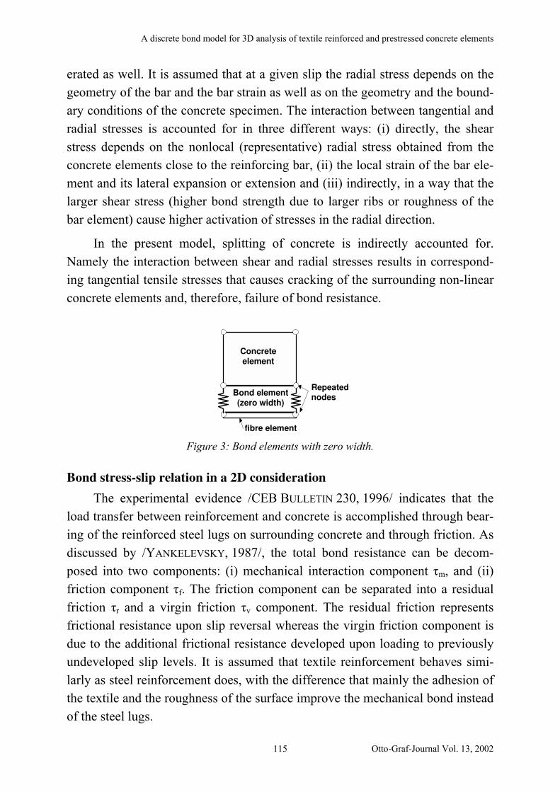
Α δισχρετε βονδ µοδελ φορ 3∆ αναλψσισ οφ τεξτιλε ρεινφορχεδ ανδ πρεστρεσσεδ χονχρετε ελεµεντσ
ερατεδ ασ ωελλ. Ιτ ισ ασσυµεδ τηατ ατ α γιϖεν σλιπ τηε ραδιαλ στρεσσ δεπενδσ ον τηε
γεοµετρψ οφ τηε βαρ ανδ τηε βαρ στραιν ασ ωελλ ασ ον τηε γεοµετρψ ανδ τηε βουνδ−
αρψ χονδιτιονσ οφ τηε χονχρετε σπεχιµεν. Τηε ιντεραχτιον βετωεεν τανγεντιαλ ανδ
ραδιαλ στρεσσεσ ισ αχχουντεδ φορ ιν τηρεε διφφερεντ ωαψσ: (ι) διρεχτλψ, τηε σηεαρ
στρεσσ δεπενδσ ον τηε νονλοχαλ (ρεπρεσεντατιϖε) ραδιαλ στρεσσ οβταινεδ φροµ τηε
χονχρετε ελεµεντσ χλοσε το τηε ρεινφορχινγ βαρ, (ιι) τηε λοχαλ στραιν οφ τηε βαρ ελε−
µεντ ανδ ιτσ λατεραλ εξπανσιον ορ εξτενσιον ανδ (ιιι) ινδιρεχτλψ, ιν α ωαψ τηατ τηε
λαργερ σηεαρ στρεσσ (ηιγηερ βονδ στρενγτη δυε το λαργερ ριβσ ορ ρουγηνεσσ οφ τηε
βαρ ελεµεντ) χαυσε ηιγηερ αχτιϖατιον οφ στρεσσεσ ιν τηε ραδιαλ διρεχτιον.
Ιν τηε πρεσεντ µοδελ, σπλιττινγ οφ χονχρετε ισ ινδιρεχτλψ αχχουντεδ φορ.
Ναµελψ τηε ιντεραχτιον βετωεεν σηεαρ ανδ ραδιαλ στρεσσεσ ρεσυλτσ ιν χορρεσπονδ−
ινγ τανγεντιαλ τενσιλε στρεσσεσ τηατ χαυσεσ χραχκινγ οφ τηε συρρουνδινγ νον−λινεαρ
χονχρετε ελεµεντσ ανδ, τηερεφορε, φαιλυρε οφ βονδ ρεσιστανχε.
Concrete element
fibre element
Bond element(zero width)
Repeated nodes
Φιγυρε 3: Βονδ ελεµεντσ ωιτη ζερο ωιδτη.
Bond stress-slip relation in a 2D consideration
Τηε εξπεριµενταλ εϖιδενχε /ΧΕΒ ΒΥΛΛΕΤΙΝ 230, 1996/ ινδιχατεσ τηατ τηε
λοαδ τρανσφερ βετωεεν ρεινφορχεµεντ ανδ χονχρετε ισ αχχοµπλισηεδ τηρουγη βεαρ−
ινγ οφ τηε ρεινφορχεδ στεελ λυγσ ον συρρουνδινγ χονχρετε ανδ τηρουγη φριχτιον. Ασ
δισχυσσεδ βψ /ΨΑΝΚΕΛΕςΣΚΨ, 1987/, τηε τοταλ βονδ ρεσιστανχε χαν βε δεχοµ−
ποσεδ ιντο τωο χοµπονεντσ: (ι) µεχηανιχαλ ιντεραχτιον χοµπονεντ !µ, ανδ (ιι)
φριχτιον χοµπονεντ !φ. Τηε φριχτιον χοµπονεντ χαν βε σεπαρατεδ ιντο α ρεσιδυαλ
φριχτιον !ρ ανδ α ϖιργιν φριχτιον !ϖ χοµπονεντ. Τηε ρεσιδυαλ φριχτιον ρεπρεσεντσ
φριχτιοναλ ρεσιστανχε υπον σλιπ ρεϖερσαλ ωηερεασ τηε ϖιργιν φριχτιον χοµπονεντ ισ
δυε το τηε αδδιτιοναλ φριχτιοναλ ρεσιστανχε δεϖελοπεδ υπον λοαδινγ το πρεϖιουσλψ
υνδεϖελοπεδ σλιπ λεϖελσ. Ιτ ισ ασσυµεδ τηατ τεξτιλε ρεινφορχεµεντ βεηαϖεσ σιµι−
λαρλψ ασ στεελ ρεινφορχεµεντ δοεσ, ωιτη τηε διφφερενχε τηατ µαινλψ τηε αδηεσιον οφ
τηε τεξτιλε ανδ τηε ρουγηνεσσ οφ τηε συρφαχε ιµπροϖε τηε µεχηανιχαλ βονδ ινστεαδ
οφ τηε στεελ λυγσ.
Οττο−Γραφ−ϑουρναλ ςολ. 13, 2002 115
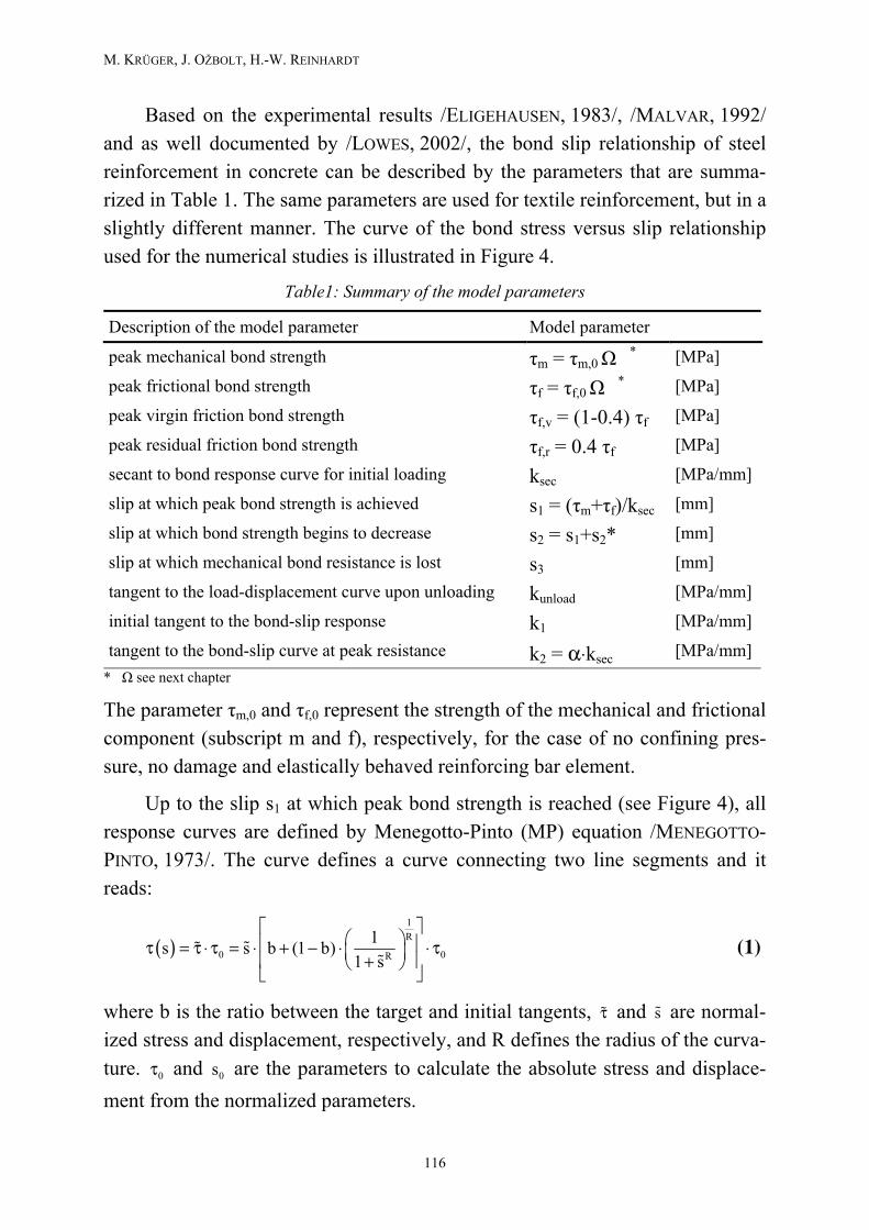
Μ. ΚΡ⇐ΓΕΡ, ϑ. ΟΒΟΛΤ, Η.−Ω. ΡΕΙΝΗΑΡ∆Τ
Βασεδ ον τηε εξπεριµενταλ ρεσυλτσ /ΕΛΙΓΕΗΑΥΣΕΝ, 1983/, /ΜΑΛςΑΡ, 1992/
ανδ ασ ωελλ δοχυµεντεδ βψ /ΛΟΩΕΣ, 2002/, τηε βονδ σλιπ ρελατιονσηιπ οφ στεελ
ρεινφορχεµεντ ιν χονχρετε χαν βε δεσχριβεδ βψ τηε παραµετερσ τηατ αρε συµµα−
ριζεδ ιν Ταβλε 1. Τηε σαµε παραµετερσ αρε υσεδ φορ τεξτιλε ρεινφορχεµεντ, βυτ ιν α
σλιγητλψ διφφερεντ µαννερ. Τηε χυρϖε οφ τηε βονδ στρεσσ ϖερσυσ σλιπ ρελατιονσηιπ
υσεδ φορ τηε νυµεριχαλ στυδιεσ ισ ιλλυστρατεδ ιν Φιγυρε 4.
Ταβλε1: Συµµαρψ οφ τηε µοδελ παραµετερσ
∆εσχριπτιον οφ τηε µοδελ παραµετερ Μοδελ παραµετερ
πεακ µεχηανιχαλ βονδ στρενγτη !µ = !µ,0 ∀ ∗ [ΜΠα]
πεακ φριχτιοναλ βονδ στρενγτη !φ = !φ,0 ∀ ∗ [ΜΠα]
πεακ ϖιργιν φριχτιον βονδ στρενγτη !φ,ϖ = (1−0.4) !φ [ΜΠα]
πεακ ρεσιδυαλ φριχτιον βονδ στρενγτη !φ,ρ = 0.4 !φ [ΜΠα]
σεχαντ το βονδ ρεσπονσε χυρϖε φορ ινιτιαλ λοαδινγ κσεχ [ΜΠα/µµ]
σλιπ ατ ωηιχη πεακ βονδ στρενγτη ισ αχηιεϖεδ σ1 = (!µ+!φ)/κσεχ [µµ]
σλιπ ατ ωηιχη βονδ στρενγτη βεγινσ το δεχρεασε σ2 = σ1+σ2∗ [µµ]
σλιπ ατ ωηιχη µεχηανιχαλ βονδ ρεσιστανχε ισ λοστ σ3 [µµ]
τανγεντ το τηε λοαδ−δισπλαχεµεντ χυρϖε υπον υνλοαδινγ κυνλοαδ [ΜΠα/µµ]
ινιτιαλ τανγεντ το τηε βονδ−σλιπ ρεσπονσε κ1 [ΜΠα/µµ]
τανγεντ το τηε βονδ−σλιπ χυρϖε ατ πεακ ρεσιστανχε κ2 = α⋅κσεχ [ΜΠα/µµ]
∗ ∀ σεε νεξτ χηαπτερ
Τηε παραµετερ !µ,0 ανδ !φ,0 ρεπρεσεντ τηε στρενγτη οφ τηε µεχηανιχαλ ανδ φριχτιοναλ
χοµπονεντ (συβσχριπτ µ ανδ φ), ρεσπεχτιϖελψ, φορ τηε χασε οφ νο χονφινινγ πρεσ−
συρε, νο δαµαγε ανδ ελαστιχαλλψ βεηαϖεδ ρεινφορχινγ βαρ ελεµεντ.
Υπ το τηε σλιπ σ1 ατ ωηιχη πεακ βονδ στρενγτη ισ ρεαχηεδ (σεε Φιγυρε 4), αλλ
ρεσπονσε χυρϖεσ αρε δεφινεδ βψ Μενεγοττο−Πιντο (ΜΠ) εθυατιον /ΜΕΝΕΓΟΤΤΟ−
ΠΙΝΤΟ, 1973/. Τηε χυρϖε δεφινεσ α χυρϖε χοννεχτινγ τωο λινε σεγµεντσ ανδ ιτ
ρεαδσ:
( )
1
Ρ
0 Ρ
1σ σ β (1 β)
1 σ 0
! ∀# ∃% &τ = τ ⋅ τ = ⋅ + − ⋅ ⋅ τ∋ (% &+) ∗
+ ,
!!!
(1)
ωηερε β ισ τηε ρατιο βετωεεν τηε ταργετ ανδ ινιτιαλ τανγεντσ, ανδ σ αρε νορµαλ−
ιζεδ στρεσσ ανδ δισπλαχεµεντ, ρεσπεχτιϖελψ, ανδ Ρ δεφινεσ τηε ραδιυσ οφ τηε χυρϖα−
τυρε. ανδ σ αρε τηε παραµετερσ το χαλχυλατε τηε αβσολυτε στρεσσ ανδ δισπλαχε−
µεντ φροµ τηε νορµαλιζεδ παραµετερσ.
τ! !
0τ 0
116
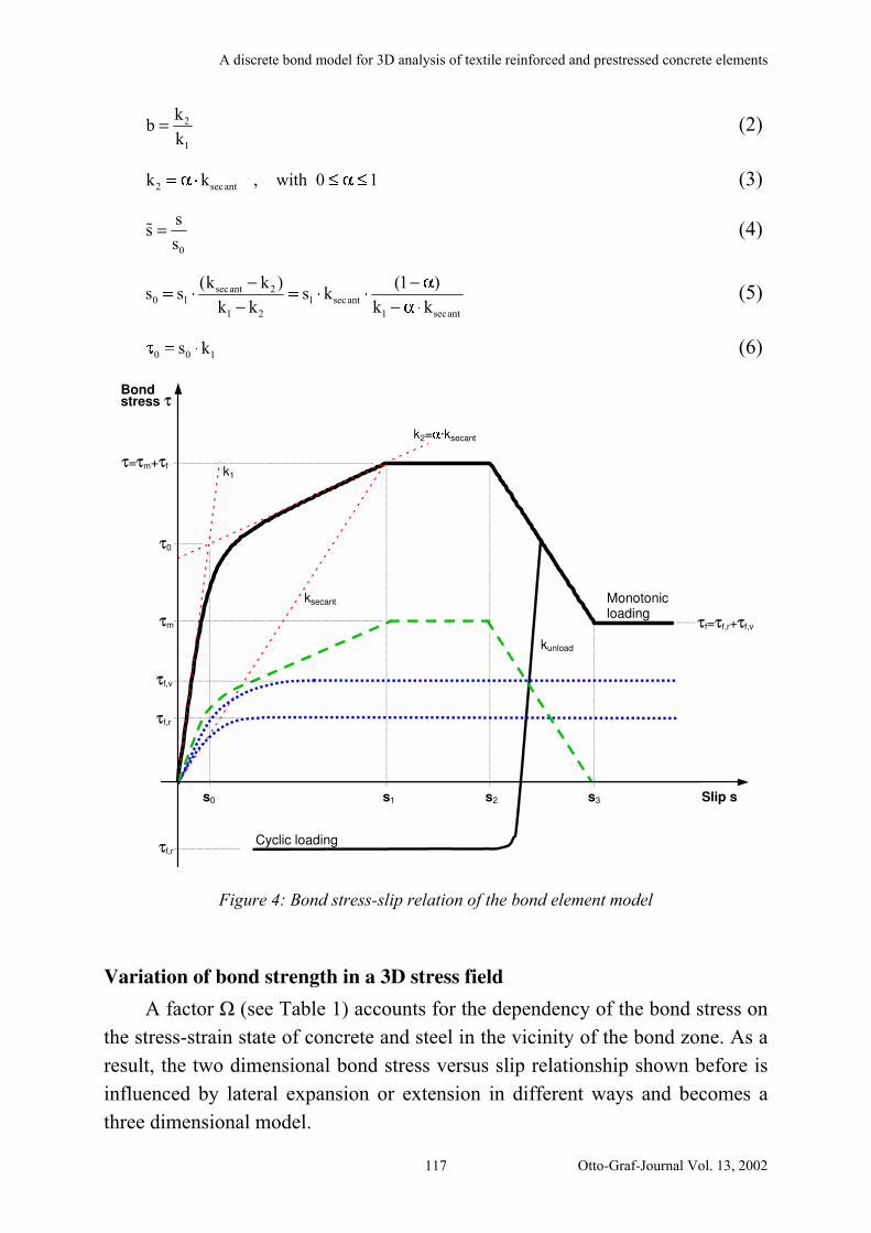
Α δισχρετε βονδ µοδελ φορ 3∆ αναλψσισ οφ τεξτιλε ρεινφορχεδ ανδ πρεστρεσσεδ χονχρετε ελεµεντσ
2
1
κβ
κ= (2)
2 σεχαντκ κ , ωιτη 0=α⋅ ≤α≤1 (3)
0
σσ
σ=! (4)
σεχαντ 20 1 1 σεχαντ
1 2 1 σεχαντ
(κ κ ) (1 )σ σ σ κ
κ κ κ κ
−=⋅ =⋅⋅− −
−αα⋅
1
(5)
0 0σ κτ=⋅ (6)
k1
k2=α·ksecant
ksecant
= m+ f
kunload
Cyclic loading
Monotonic loading
s1 s3 Slip s s2
f,r
m
f,v
f= f,r+ f,v
Bond stress
s0
0
f,r
Φιγυρε 4: Βονδ στρεσσ−σλιπ ρελατιον οφ τηε βονδ ελεµεντ µοδελ
Variation of bond strength in a 3D stress field
Α φαχτορ ∀ (σεε Ταβλε 1) αχχουντσ φορ τηε δεπενδενχψ οφ τηε βονδ στρεσσ ον
τηε στρεσσ−στραιν στατε οφ χονχρετε ανδ στεελ ιν τηε ϖιχινιτψ οφ τηε βονδ ζονε. Ασ α
ρεσυλτ, τηε τωο διµενσιοναλ βονδ στρεσσ ϖερσυσ σλιπ ρελατιονσηιπ σηοων βεφορε ισ
ινφλυενχεδ βψ λατεραλ εξπανσιον ορ εξτενσιον ιν διφφερεντ ωαψσ ανδ βεχοµεσ α
τηρεε διµενσιοναλ µοδελ.
Οττο−Γραφ−ϑουρναλ ςολ. 13, 2002 117
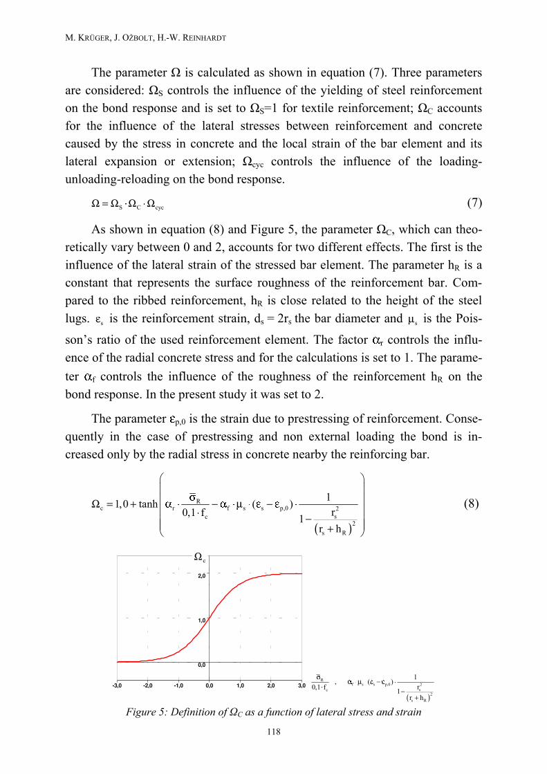
Μ. ΚΡ⇐ΓΕΡ, ϑ. ΟΒΟΛΤ, Η.−Ω. ΡΕΙΝΗΑΡ∆Τ
Τηε παραµετερ ∀ ισ χαλχυλατεδ ασ σηοων ιν εθυατιον (7). Τηρεε παραµετερσ
αρε χονσιδερεδ: ∀Σ χοντρολσ τηε ινφλυενχε οφ τηε ψιελδινγ οφ στεελ ρεινφορχεµεντ
ον τηε βονδ ρεσπονσε ανδ ισ σετ το ∀Σ=1 φορ τεξτιλε ρεινφορχεµεντ; ∀Χ αχχουντσ
φορ τηε ινφλυενχε οφ τηε λατεραλ στρεσσεσ βετωεεν ρεινφορχεµεντ ανδ χονχρετε
χαυσεδ βψ τηε στρεσσ ιν χονχρετε ανδ τηε λοχαλ στραιν οφ τηε βαρ ελεµεντ ανδ ιτσ
λατεραλ εξπανσιον ορ εξτενσιον; ∀χψχ χοντρολσ τηε ινφλυενχε οφ τηε λοαδινγ−
υνλοαδινγ−ρελοαδινγ ον τηε βονδ ρεσπονσε.
Σ Χ χψΩ = Ω⋅Ω⋅Ω χ (7)
Ασ σηοων ιν εθυατιον (8) ανδ Φιγυρε 5, τηε παραµετερ ∀Χ, ωηιχη χαν τηεο−
ρετιχαλλψ ϖαρψ βετωεεν 0 ανδ 2, αχχουντσ φορ τωο διφφερεντ εφφεχτσ. Τηε φιρστ ισ τηε
ινφλυενχε οφ τηε λατεραλ στραιν οφ τηε στρεσσεδ βαρ ελεµεντ. Τηε παραµετερ ηΡ ισ α
χονσταντ τηατ ρεπρεσεντσ τηε συρφαχε ρουγηνεσσ οφ τηε ρεινφορχεµεντ βαρ. Χοµ−
παρεδ το τηε ριββεδ ρεινφορχεµεντ, ηΡ ισ χλοσε ρελατεδ το τηε ηειγητ οφ τηε στεελ
λυγσ. ισ τηε ρεινφορχεµεντ στραιν, δσε
σ = 2ρσ τηε βαρ διαµετερ ανδ σµ ισ τηε Ποισ−
σονσ ρατιο οφ τηε υσεδ ρεινφορχεµεντ ελεµεντ. Τηε φαχτορ αρ χοντρολσ τηε ινφλυ−
ενχε οφ τηε ραδιαλ χονχρετε στρεσσ ανδ φορ τηε χαλχυλατιονσ ισ σετ το 1. Τηε παραµε−
τερ αφ χοντρολσ τηε ινφλυενχε οφ τηε ρουγηνεσσ οφ τηε ρεινφορχεµεντ ηΡ ον τηε
βονδ ρεσπονσε. Ιν τηε πρεσεντ στυδψ ιτ ωασ σετ το 2.
Τηε παραµετερ επ,0 ισ τηε στραιν δυε το πρεστρεσσινγ οφ ρεινφορχεµεντ. Χονσε−
θυεντλψ ιν τηε χασε οφ πρεστρεσσινγ ανδ νον εξτερναλ λοαδινγ τηε βονδ ισ ιν−
χρεασεδ ονλψ βψ τηε ραδιαλ στρεσσ ιν χονχρετε νεαρβψ τηε ρεινφορχινγ βαρ.
( )
Ρχ ρ φ σ σ π,0 2
σχ2
σ Ρ
11,0 τανη ( )
ρ0,1 φ1
ρ η
# ∃∋ (σ∋Ω = + α⋅ −α⋅µ⋅ε−ε⋅∋ ⋅
−∋ (∋ (+) ∗
((
(8)
-3,0 -2,0 -1,0 0,0 1,0 2,0 3,0
0,0
1,0
2,0
( )
Ρφ σ σ π,0 2
σχ2
σ Ρ
1, ( )
ρ0,1 φ1
ρ η
σ−α⋅µ⋅ε−ε⋅⋅−
+
χΩ
Φιγυρε 5: ∆εφινιτιον οφ !Χ ασ α φυνχτιον οφ λατεραλ στρεσσ ανδ στραιν
118

Α δισχρετε βονδ µοδελ φορ 3∆ αναλψσισ οφ τεξτιλε ρεινφορχεδ ανδ πρεστρεσσεδ χονχρετε ελεµεντσ
Τηε ινφλυενχε οφ τηε ραδιαλ στρεσσ ιν χονχρετε ιν τηε ϖιχινιτψ οφ τηε ρεινφορχ−
ινγ βαρ ισ αχχουντεδ φορ βψ αν αϖεραγε ραδιαλ στρεσσ ρσ περπενδιχυλαρ το τηε βαρ
διρεχτιον. Τηε παραµετερ φχ ισ τηε υνιαξιαλ χοµπρεσσιϖε στρενγτη οφ χονχρετε. Ιν
τηε φινιτε ελεµεντ αναλψσισ τηε αϖεραγε ραδιαλ στρεσσ ασσοχιατεδ το τηε ν−τη βαρ
ελεµεντ ισ χαλχυλατεδ ασ:
Ν Νι
ρ ρ ι Ρι 1 ι 1Ρ
ωιτη1
ς ςς = =
σ = σ ∆ = ∆− ις− (9)
ωηερε ∆ ςι δενοτεσ τηε ϖολυµε ωηιχη χορρεσπονδσ το τηε ι−τη ιντεγρατιον
ποιντ οφ τηε φινιτε ελεµεντ ανδ τηε στρεσσ περπενδιχυλαρ το τηε ρεινφορχεµεντ.
Ν ισ α τοταλ νυµβερ οφ ιντεγρατιον ποιντσ τηατ φαλλ ιντο α χψλινδερ οφ α διαµετερ ∆
(σεε Φιγυρε 6). Ιν τηε πρεσεντεδ µοδελ ∆ ισ ασσυµεδ το βε τηρεε τιµεσ α βαρ δι−
αµετερ (∆ ≈ 3 δ
ιρσ
σ). Ιν (9) ςΡ ισ τηε ρεπρεσεντατιϖε ϖολυµε, ι.ε. τηε ϖολυµε οφ τηε
χονχρετε χψλινδερ οφ διαµετερ ∆ τηατ ισ ασσοχιατεδ το τηε τρυσσ φινιτε ελεµεντ
ωηιχη ρεπρεσεντσ α ρεινφορχινγ βαρ.
Φιγυρε 6: Ρεπρεσεντατιϖε ϖολυµε
Εξπεριµεντσ σηοω τηατ φορ χψχλινγ λοαδινγ−υνλοαδινγ−ρελοαδινγ τηε βονδ
στρενγτη σιγνιφιχαντλψ δεχρεασεσ ωιτη ινχρεασε οφ νυµβερ οφ λοαδινγ χψχλεσ
/ΕΛΙΓΕΗΑΥΣΕΝ, 1983/, /ΒΑΛΑΖΣ, 1991/. Ιν τηε πρεσεντ µοδελ τηισ εφφεχτ ισ αχ−
χουντεδ φορ βψ τηε φαχτορ ∀χψχ τηατ ρεαδσ:
1.1
χψχ0
εξπ 1.2# # ∃Λ∋Ω = − ⋅ ∋ (∋ Λ) ∗) ∗
∃((
(10)
ωηερε # ισ τηε αχχυµυλατεδ σηεαρ ενεργψ δισσιπατιον ανδ #0 ισ α χονσταντ
ρεπρεσεντινγ τηε αρεα υνδερ τηε µονοτονιχ βονδ−σλιπ χυρϖε οφ ρεσπεχτιϖε σηεαρ
χοµπονεντ. Τηε αβοϖε εθυατιον ηασ βεεν προποσεδ βψ /ΕΛΙΓΕΗΑΥΣΕΝ, 1983/ ανδ
ιτ ισ βασεδ ον α λαργε νυµβερ οφ χψχλιχ τεστ δατα οφ στεελ ρεινφορχεδ χονχρετε.
Οττο−Γραφ−ϑουρναλ ςολ. 13, 2002 119

Μ. ΚΡ⇐ΓΕΡ, ϑ. ΟΒΟΛΤ, Η.−Ω. ΡΕΙΝΗΑΡ∆Τ
Σιµιλαρ βεηαϖιορ σεεµσ αλσο το βε αππροξιµατελψ ϖαλιδ φορ τεξτιλε ρεινφορχεδ χον−
χρετε, ηοωεϖερ, ιτ ισ νοτ χλαριφιεδ υπ το νοω.
NUMERICAL STUDIES
Ασ σηοων ιν τηε λαστ χηαπτερ τηε βονδ περφορµανχε οφ τηε µοδελ ισ ινφλυ−
ενχεδ βψ ∀Χ ωηιχη αχχουντσ φορ: (ι) τηε ινφλυενχε οφ ραδιαλ στρεσσ οβταινεδ φροµ
τηε συρρουνδινγ χονχρετε ελεµεντσ ανδ (ιι) τηε ινφλυενχε οφ ρεινφορχεµεντ στραιν.
Το δεµονστρατε τηε εφφεχτσ οφ τηεσε τωο διφφερεντ ινφλυενχεσ νυµεριχαλ στυδιεσ
ηαϖε βεεν χαρριεδ ουτ.
Τωο ΦΕ µοδελσ (ΜΙ ανδ ΜΙΙ) ωερε εµπλοψεδ το σηοω τηε ινφλυενχε οφ τηε
τρανσϖερσε στρεσσ φιελδ ανδ τηε ρεινφορχεµεντ στραιν ον τηε βονδ προπερτιεσ. Τηε
ΦΕ µεση οφ τηεσε µοδελσ ισ σηοων ιν Φιγυρε 7. Ιτ ρεπρεσεντσ χονχρετε σπεχιµεν
χονφινεδ ιν διρεχτιον ξ ανδ ψ. Τηε βουνδαρψ χονδιτιονσ ωερε σλιγητλψ διφφερεντ.
Μοδελ Ι (ΜΙ) ηασ σοµε ρεστραινεδ νοδεσ ιν τηε ζ−διρεχτιον ονλψ ατ τηε βοττοµ συρ−
φαχε, ωηερε τηε λοαδ ισ αππλιεδ το τηε βαρ ελεµεντ. Ιν Μοδελ ΙΙ (ΜΙΙ) αλλ τηε νοδεσ
οϖερ τηε σπεχιµεν ηειγητ ωερε φιξεδ ιν τηε ζ−διρεχτιον. Χονσεθυεντλψ, τηε τρανσ−
ϖερσε στρεσσ φιελδ αρουνδ τηε βαρ ελεµεντ ισ διφφερεντ. Τηε βαρ ελεµεντ ιτσελφ ισ
πλαχεδ ιν τηε µιδδλε οφ τηε σπεχιµεν ανδ ισ πυλλεδ ιν ζ διρεχτιον ατ τηε ποιντ
ζ = 20 µµ (βοττοµ συρφαχε).
Φιγυρε 7: Φινιτε ελεµεντ µοδελσ ωιτη διφφερεντ βουνδαρψ χονδιτιονσ
Ασ σηοων ιν ταβλε 2, τηε µαιν βονδ παραµετερσ ωερε σετ το χονσταντ φορ αλλ
χαλχυλατιονσ. Νοτε τηατ τηεσε παραµετερσ ωερε χηοσεν ονλψ το θυαλιτατιϖελψ σηοω
τηε περφορµανχε οφ τηε µοδελ ανδ ωερε νοτ χαλιβρατεδ φορ τηε υσε ιν τηε πραχτιχαλ
120

Α δισχρετε βονδ µοδελ φορ 3∆ αναλψσισ οφ τεξτιλε ρεινφορχεδ ανδ πρεστρεσσεδ χονχρετε ελεµεντσ
αππλιχατιονσ. Αδδιτιοναλλψ, ιτ ηασ το βε νοτεδ τηατ τηε ρεινφορχεµεντ ισ ασσυµεδ
το βε λινεαρ ελαστιχ φορ αλλ τηε χαλχυλατιονσ, ι.ε. ∀Σ = 1.
Ταβλε2: Συµµαρψ οφ τηε υσεδ µοδελ παραµετερσ φορ τηε ρεινφορχεµεντ
∆εσχριπτιον οφ τηε µοδελ παραµετερ Μοδελ παραµετερ
πεακ µεχηανιχαλ βονδ στρενγτη !µ = 9.0 [ΜΠα]
πεακ φριχτιοναλ βονδ στρενγτη !φ = 4.0 [ΜΠα]
σεχαντ το βονδ ρεσπονσε χυρϖε φορ ινιτιαλ λοαδινγ κσεχ = 50.0 [ΜΠα/µµ]
σλιπ ατ ωηιχη βονδ στρενγτη βεγινσ το δεχρεασε σ2∗ = 0.03 [µµ]
σλιπ ατ ωηιχη µεχηανιχαλ βονδ ρεσιστανχε ισ λοστ σ3 = 0.50 [µµ]
τανγεντ το τηε λοαδ−δισπλαχεµεντ χυρϖε υπον υνλοαδινγ κυνλοαδ = 220.0 [ΜΠα/µµ]
ινιτιαλ τανγεντ το τηε βονδ−σλιπ ρεσπονσε κ1 = 220.0 [ΜΠα/µµ]
τανγεντ το τηε βονδ−σλιπ χυρϖε ατ πεακ ρεσιστανχε κ2 = 22.0 [ΜΠα/µµ]
ραδιυσ οφ τηε χυρϖατυρε Ρ = 8.0 [−]
Ποισσονσ ρατιο µσ = 0.5 [−]
Ψουνγ µοδυλυσ Εσ = 74000.0 [ΜΠα]
ρεινφορχεµεντ αρεα Ασ = 0.93 [µµ″]
βαρ διαµετερ 2 ⋅ ρσ = 1.0 [µµ]
συρφαχε ρουγηνεσσ ηΡ = 0.01 [µµ]
Μορεοϖερ, το δεµονστρατε τηε εφφεχτ οφ πρεστρεσσινγ, τηρεε διφφερεντ χασεσ
(α,β,χ) ωερε χονσιδερεδ ωιτη:
(α) (11) Χ,α 1.0Ω =
(β) ΡΧ,β
χ
1.0 τανη0,1 φ
#σΩ = + ∋ ⋅
) ∗
∃( (12)
(χ)
( )
ΡΧ,χ φ σ σ π,0 2
σχ2
σ Ρ
11.0 τανη ( )
ρ0,1 φ1
ρ η
# ∃∋ (σ∋Ω = + −α⋅µ⋅ε−ε⋅
∋ ⋅−∋ (∋ (+) ∗
(( (13)
Influence of the 3D stress field on the bond
Ιν Φιγυρε 8 τηε ρεσυλτσ οφ τηε πυλλ ουτ στρεσσ ϖερσυσ σλιπ αρε σηοων. Ιν τηε
χασε (α) τηε στρεσσ ϖερσυσ σλιπ χυρϖε οφ βοτη µοδελσ λοοκσ αλµοστ τηε σαµε φορ
πρεστρεσσεδ ανδ νον πρεστρεσσεδ στατε, ι.ε. τηε χονχρετε στραιν ιν ζ διρεχτιον ισ
νεγλιγιβλε. Τηερεφορε ιτ ισ σηοων ονλψ ονε χυρϖε. Ηοωεϖερ, ιτ χαν βε σεεν τηατ ιφ
Οττο−Γραφ−ϑουρναλ ςολ. 13, 2002 121
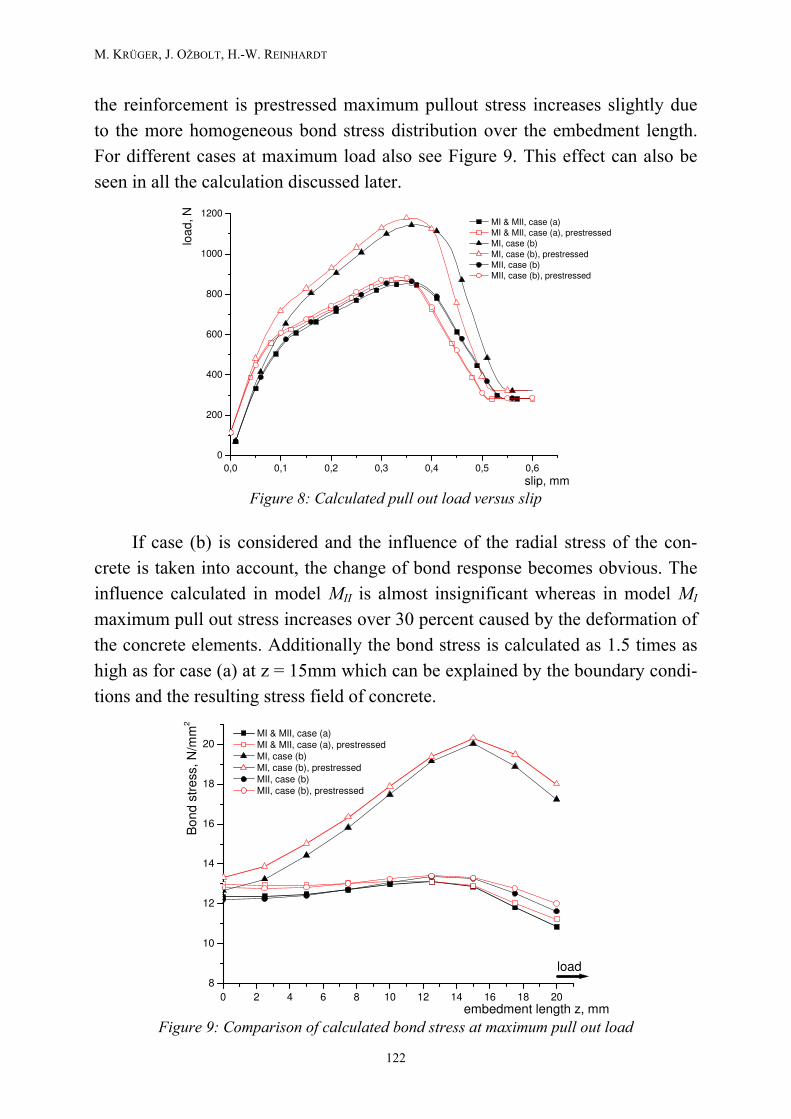
Μ. ΚΡ⇐ΓΕΡ, ϑ. ΟΒΟΛΤ, Η.−Ω. ΡΕΙΝΗΑΡ∆Τ
τηε ρεινφορχεµεντ ισ πρεστρεσσεδ µαξιµυµ πυλλουτ στρεσσ ινχρεασεσ σλιγητλψ δυε
το τηε µορε ηοµογενεουσ βονδ στρεσσ διστριβυτιον οϖερ τηε εµβεδµεντ λενγτη.
Φορ διφφερεντ χασεσ ατ µαξιµυµ λοαδ αλσο σεε Φιγυρε 9. Τηισ εφφεχτ χαν αλσο βε
σεεν ιν αλλ τηε χαλχυλατιον δισχυσσεδ λατερ.
0,0 0,1 0,2 0,3 0,4 0,5 0,6
0
200
400
600
800
1000
1200 MI & MII, case (a) MI & MII, case (a), prestressed MI, case (b)
MI, case (b), prestressed MII, case (b) MII, case (b), prestressed
loa
d, N
slip, mm Φιγυρε 8: Χαλχυλατεδ πυλλ ουτ λοαδ ϖερσυσ σλιπ
Ιφ χασε (β) ισ χονσιδερεδ ανδ τηε ινφλυενχε οφ τηε ραδιαλ στρεσσ οφ τηε χον−
χρετε ισ τακεν ιντο αχχουντ, τηε χηανγε οφ βονδ ρεσπονσε βεχοµεσ οβϖιουσ. Τηε
ινφλυενχε χαλχυλατεδ ιν µοδελ ΜΙΙ ισ αλµοστ ινσιγνιφιχαντ ωηερεασ ιν µοδελ ΜΙ
µαξιµυµ πυλλ ουτ στρεσσ ινχρεασεσ οϖερ 30 περχεντ χαυσεδ βψ τηε δεφορµατιον οφ
τηε χονχρετε ελεµεντσ. Αδδιτιοναλλψ τηε βονδ στρεσσ ισ χαλχυλατεδ ασ 1.5 τιµεσ ασ
ηιγη ασ φορ χασε (α) ατ ζ = 15µµ ωηιχη χαν βε εξπλαινεδ βψ τηε βουνδαρψ χονδι−
τιονσ ανδ τηε ρεσυλτινγ στρεσσ φιελδ οφ χονχρετε.
0 2 4 6 8 10 12 14 16 18 20
8
10
12
14
16
18
20
load
MI & MII, case (a) MI & MII, case (a), prestressed MI, case (b) MI, case (b), prestressed MII, case (b) MII, case (b), prestressed
Bo
nd
str
ess, N
/mm
2
embedment length z, mm Φιγυρε 9: Χοµπαρισον οφ χαλχυλατεδ βονδ στρεσσ ατ µαξιµυµ πυλλ ουτ λοαδ
122
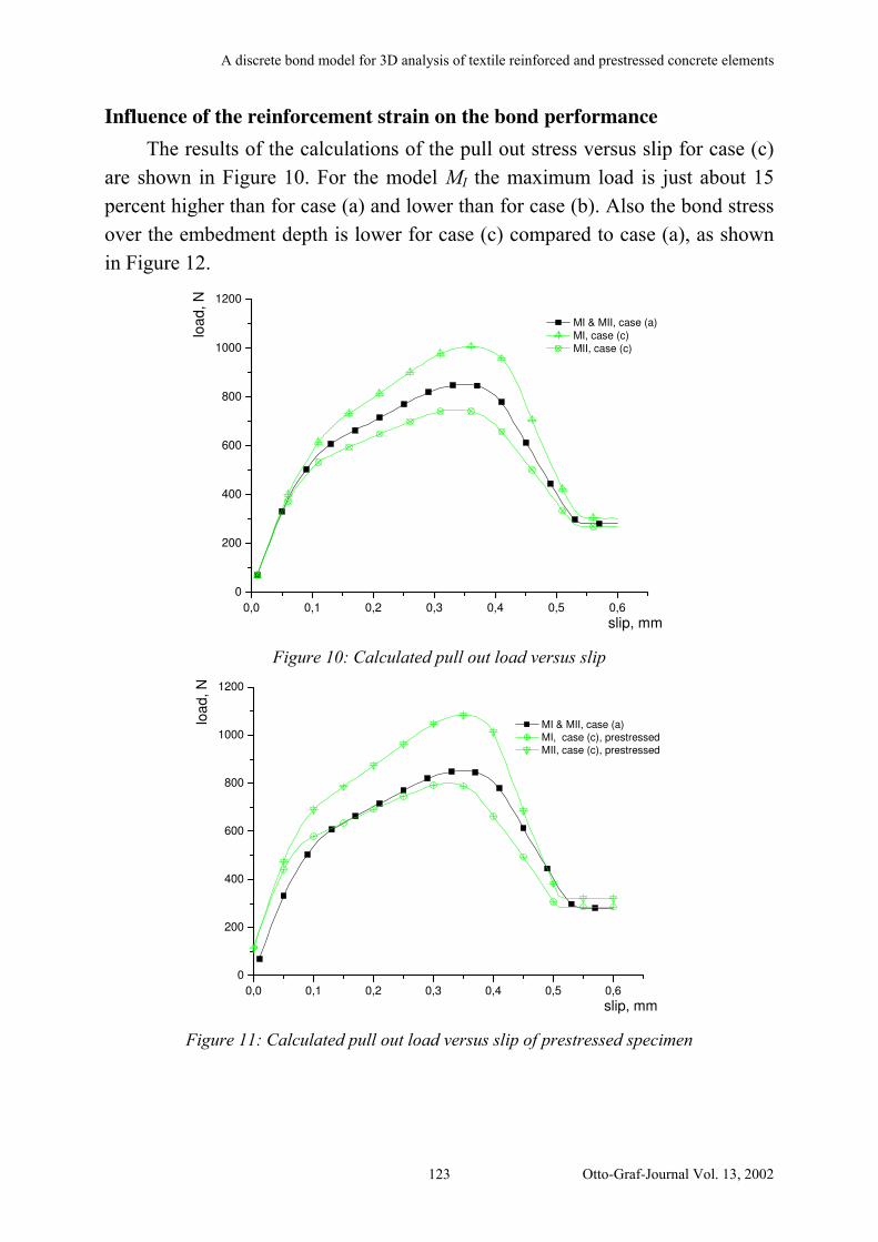
Α δισχρετε βονδ µοδελ φορ 3∆ αναλψσισ οφ τεξτιλε ρεινφορχεδ ανδ πρεστρεσσεδ χονχρετε ελεµεντσ
Influence of the reinforcement strain on the bond performance
Τηε ρεσυλτσ οφ τηε χαλχυλατιονσ οφ τηε πυλλ ουτ στρεσσ ϖερσυσ σλιπ φορ χασε (χ)
αρε σηοων ιν Φιγυρε 10. Φορ τηε µοδελ ΜΙ τηε µαξιµυµ λοαδ ισ ϕυστ αβουτ 15
περχεντ ηιγηερ τηαν φορ χασε (α) ανδ λοωερ τηαν φορ χασε (β). Αλσο τηε βονδ στρεσσ
οϖερ τηε εµβεδµεντ δεπτη ισ λοωερ φορ χασε (χ) χοµπαρεδ το χασε (α), ασ σηοων
ιν Φιγυρε 12.
0,0 0,1 0,2 0,3 0,4 0,5 0,6
0
200
400
600
800
1000
1200
MI & MII, case (a) MI, case (c) MII, case (c)
loa
d, N
slip, mm
Φιγυρε 10: Χαλχυλατεδ πυλλ ουτ λοαδ ϖερσυσ σλιπ
0,0 0,1 0,2 0,3 0,4 0,5 0,6
0
200
400
600
800
1000
1200
MI & MII, case (a)
MI, case (c), prestressed MII, case (c), prestressed
loa
d, N
slip, mm
Φιγυρε 11: Χαλχυλατεδ πυλλ ουτ λοαδ ϖερσυσ σλιπ οφ πρεστρεσσεδ σπεχιµεν
Οττο−Γραφ−ϑουρναλ ςολ. 13, 2002 123

Μ. ΚΡ⇐ΓΕΡ, ϑ. ΟΒΟΛΤ, Η.−Ω. ΡΕΙΝΗΑΡ∆Τ
Ιν τηε χαλχυλατεδ βονδ στρεσσ σλιπ χυρϖεσ φορ πρεστρεσσεδ ρεινφορχεµεντσ,
σηοων ιν Φιγυρε 11, τηε ινφλυενχε οφ τηε στεελ στραιν ον τηε βονδ περφορµανχε ισ
αλσο οβϖιουσ. ∆υε το τηε πρεστρεσσινγ οφ αδηεσιϖε τψπε, ατ ινιτιαλ στατε τηε ρειν−
φορχεµεντ λατεραλ στραινσ αρε νεγατιϖε (χοµπρεσσιον). Χονσεθυεντλψ, τηε χοντραχ−
τιον οφ ρεινφορχεµεντ ισ λεσσ τηαν ιν τηε χασε οφ υνπρεστρεσσεδ ρεινφορχεµεντ ανδ
τηερεφορε ιτ δοεσ νοτ ρεσυλτ ιν συχη α λαργε ρεδυχτιον οφ βονδ στρεσσεσ. Φιγυρε 12
σηοωσ τηε ινφλυενχε οφ ∀Χ ον τηε βονδ στρεσσ φορ υνπρεστρεσσεδ ανδ πρεστρεσσεδ
ρεινφορχεµεντ.
0 2 4 6 8 10 12 14 16 18 20
8
10
12
14
16
18
20
load
MI & MII, case (a) MI & MII, case (a), prestressed MI, case (c) MI, case (c), prestressed MII, case (c) MII, case (c), prestressed
Bo
nd
str
ess, N
/mm
2
embedment length z, mm
Φιγυρε 12: Χοµπαρισον οφ χαλχυλατεδ βονδ στρεσσ ατ µαξιµυµ πυλλ ουτ λοαδ
Comparison of calculations and tests of textile reinforced elements in a bending test
Ιν Φιγυρε 13 τηε ρεσυλτ οφ α φουρ−ποιντ βενδινγ τεστ ισ χοµπαρεδ ωιτη τηε ρε−
συλτσ οφ τηε ΦΕ χαλχυλατιονσ. Τηε σπαν οφ τηε πλατε ωασ 250 µµ ανδ τηε λοαδ ωασ
αππλιεδ ατ τηε τηιρδ ποιντσ. Τηε τεστ σπεχιµεν ωασ α εποξψ ιµπρεγνατεδ χαρβον
τεξτιλε ρεινφορχεδ χονχρετε πλατε (300µµ ξ 60µµ ξ 10µµ) ωιτη α φινε γραιν
χονχρετε (φχ ≈ 80ΜΠα). Τηε ινπυτ παραµετερσ φορ τηε χαλχυλατιον οφ τηε βενδινγ
τεστ ωερε χαλιβρατεδ ατ δουβλε σιδεδ πυλλουτ τεστσ. Φορ δεταιλσ σεε /ΚΡ⇐ΓΕΡ,
2002/. Φορ τηε χαλχυλατιον χονχρετε ισ µοδελλεδ βψ τηε µιχροπλανε µοδελ. Τηε
αγρεεµεντ βετωεεν σιµυλατιον ανδ εξπεριµενταλ ρεσυλτσ ισ γοοδ. Ηοωεϖερ, χοµ−
παρεδ το τηε τεστ ρεσυλτσ, τηε νυµεριχαλ ρεσυλτσ σηοω ιν τηε ποστ πεακ ρεγιον µορε
δυχτιλε βεηαϖιουρ.
124
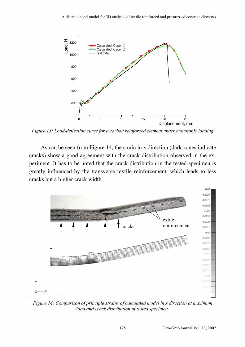
Α δισχρετε βονδ µοδελ φορ 3∆ αναλψσισ οφ τεξτιλε ρεινφορχεδ ανδ πρεστρεσσεδ χονχρετε ελεµεντσ
0 5 10 15 20 25
0
200
400
600
800
1000
1200 Calculated, Case (a) Calculated, Case (c) test data
Displacement, mm
Loa
d,
N
Φιγυρε 13: Λοαδ−δεφλεχτιον χυρϖε φορ α χαρβον ρεινφορχεδ ελεµεντ υνδερ µονοτονιχ λοαδινγ
Ασ χαν βε σεεν φροµ Φιγυρε 14, τηε στραιν ιν ξ διρεχτιον (δαρκ ζονεσ ινδιχατε
χραχκσ) σηοω α γοοδ αγρεεµεντ ωιτη τηε χραχκ διστριβυτιον οβσερϖεδ ιν τηε εξ−
περιµεντ. Ιτ ηασ το βε νοτεδ τηατ τηε χραχκ διστριβυτιον ιν τηε τεστεδ σπεχιµεν ισ
γρεατλψ ινφλυενχεδ βψ τηε τρανσϖερσε τεξτιλε ρεινφορχεµεντ, ωηιχη λεαδσ το λεσσ
χραχκσ βυτ α ηιγηερ χραχκ ωιδτη.
X
Y
Z
0.03
0.0287
0.0275
0.0262
0.025
0.0238
0.0225
0.0212
0.02
0.0187
0.0175
0.0163
0.015
0.0138
0.0125
0.0113
0.01
0.00875
0.0075
0.00625
0.005
1
utput Set: MASA3 pbzfCEP6072eformed(20.26): Total nodal disp.
χραχκσ τεξτιλε ρεινφορχεµεντ
Φιγυρε 14: Χοµπαρισον οφ πρινχιπλε στραινσ οφ χαλχυλατεδ µοδελ ιν ξ διρεχτιον ατ µαξιµυµ λοαδ ανδ χραχκ διστριβυτιον οφ τεστεδ σπεχιµεν.
Οττο−Γραφ−ϑουρναλ ςολ. 13, 2002 125
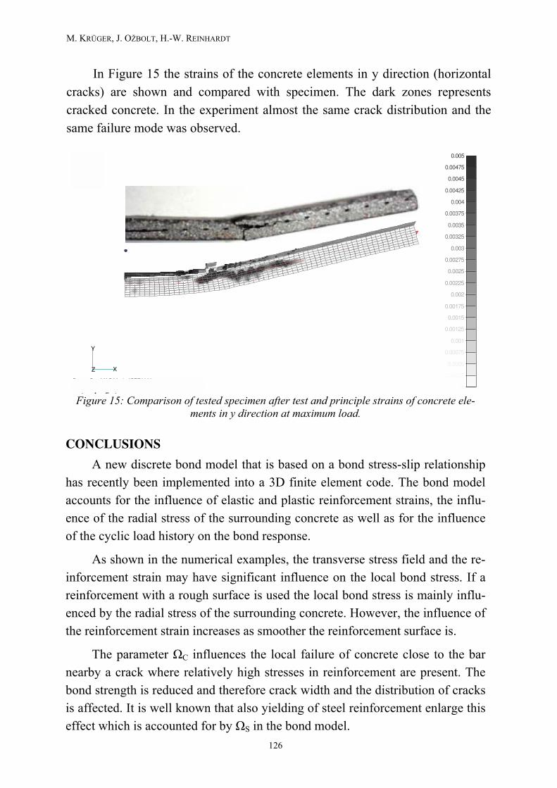
Μ. ΚΡ⇐ΓΕΡ, ϑ. ΟΒΟΛΤ, Η.−Ω. ΡΕΙΝΗΑΡ∆Τ
Ιν Φιγυρε 15 τηε στραινσ οφ τηε χονχρετε ελεµεντσ ιν ψ διρεχτιον (ηοριζονταλ
χραχκσ) αρε σηοων ανδ χοµπαρεδ ωιτη σπεχιµεν. Τηε δαρκ ζονεσ ρεπρεσεντσ
χραχκεδ χονχρετε. Ιν τηε εξπεριµεντ αλµοστ τηε σαµε χραχκ διστριβυτιον ανδ τηε
σαµε φαιλυρε µοδε ωασ οβσερϖεδ.
X
Y
Z
0.005
0.00475
0.0045
0.00425
0.004
0.00375
0.0035
0.00325
0.003
0.00275
0.0025
0.00225
0.002
0.00175
0.0015
0.00125
0.001
0.00075
0.0005
0.00025
0.
L1
C1
Output Set: MASA3 pbzfCEP6080
Deformed(22.23): Total nodal disp.
C
onto r A rg E stra
Φιγυρε 15: Χοµπαρισον οφ τεστεδ σπεχιµεν αφτερ τεστ ανδ πρινχιπλε στραινσ οφ χονχρετε ελε−µεντσ ιν ψ διρεχτιον ατ µαξιµυµ λοαδ.
CONCLUSIONS
Α νεω δισχρετε βονδ µοδελ τηατ ισ βασεδ ον α βονδ στρεσσ−σλιπ ρελατιονσηιπ
ηασ ρεχεντλψ βεεν ιµπλεµεντεδ ιντο α 3∆ φινιτε ελεµεντ χοδε. Τηε βονδ µοδελ
αχχουντσ φορ τηε ινφλυενχε οφ ελαστιχ ανδ πλαστιχ ρεινφορχεµεντ στραινσ, τηε ινφλυ−
ενχε οφ τηε ραδιαλ στρεσσ οφ τηε συρρουνδινγ χονχρετε ασ ωελλ ασ φορ τηε ινφλυενχε
οφ τηε χψχλιχ λοαδ ηιστορψ ον τηε βονδ ρεσπονσε.
Ασ σηοων ιν τηε νυµεριχαλ εξαµπλεσ, τηε τρανσϖερσε στρεσσ φιελδ ανδ τηε ρε−
ινφορχεµεντ στραιν µαψ ηαϖε σιγνιφιχαντ ινφλυενχε ον τηε λοχαλ βονδ στρεσσ. Ιφ α
ρεινφορχεµεντ ωιτη α ρουγη συρφαχε ισ υσεδ τηε λοχαλ βονδ στρεσσ ισ µαινλψ ινφλυ−
ενχεδ βψ τηε ραδιαλ στρεσσ οφ τηε συρρουνδινγ χονχρετε. Ηοωεϖερ, τηε ινφλυενχε οφ
τηε ρεινφορχεµεντ στραιν ινχρεασεσ ασ σµοοτηερ τηε ρεινφορχεµεντ συρφαχε ισ.
Τηε παραµετερ ∀Χ ινφλυενχεσ τηε λοχαλ φαιλυρε οφ χονχρετε χλοσε το τηε βαρ
νεαρβψ α χραχκ ωηερε ρελατιϖελψ ηιγη στρεσσεσ ιν ρεινφορχεµεντ αρε πρεσεντ. Τηε
βονδ στρενγτη ισ ρεδυχεδ ανδ τηερεφορε χραχκ ωιδτη ανδ τηε διστριβυτιον οφ χραχκσ
ισ αφφεχτεδ. Ιτ ισ ωελλ κνοων τηατ αλσο ψιελδινγ οφ στεελ ρεινφορχεµεντ ενλαργε τηισ
εφφεχτ ωηιχη ισ αχχουντεδ φορ βψ ∀Σ ιν τηε βονδ µοδελ.
126

Α δισχρετε βονδ µοδελ φορ 3∆ αναλψσισ οφ τεξτιλε ρεινφορχεδ ανδ πρεστρεσσεδ χονχρετε ελεµεντσ
Τηε βενεφιτ οφ τηε πρεσεντεδ βονδ µοδελ βεχοµεσ οβϖιουσ ιφ ονε χονσιδερ
διφφερεντ τψπεσ οφ ρεινφορχεµεντσ, ε.γ. διφφερεντ διαµετερ, συρφαχε στρυχτυρεσ ορ
στεελ λυγσ ανδ στρεσσ στραιν προπερτιεσ. Ιτ ισ ασσυµεδ τηατ τηε γενεραλ παραµετερσ
οφ τηε βονδ στρεσσ σλιπ−ρελατιον σηοων ιν Φιγυρε 1 µαινλψ δεπενδ ον τηε χονχρετε
παραµετερσ ανδ χαν βε σετ το χονσταντ φορ α γρουπ οφ ρεινφορχεµεντ ελεµεντσ οφ
τηε σαµε τψπε. Τηισ χαν βε φορ εξαµπλε α σετ οφ στεελ βαρσ οφ διφφερεντ διαµετερ
ορ τεξτιλε ρεινφορχεµεντ τψπε ωιτη διφφερεντ Ψουνγσ µοδυλυσ βυτ αλµοστ τηε
σαµε συρφαχε ρουγηνεσσ.
Νεϖερτηελεσσ τηε δισχυσσεδ µοδελ ηαϖε το βε χαλιβρατεδ βασεδ ον α σεριεσ οφ
διφφερεντ εξπεριµενταλ τεστσ ιν ορδερ το φινδ ουτ τηε ρεαλ ινφλυενχε οφ τρανσϖερσε
στρεσσεσ ανδ στραινσ ον τηε βονδ ρεσπονσε ανδ τηυσ ον τηε στρυχτυραλ ρεσπονσε ασ
ωελλ.
REFERENCES
Βαλαζσ, Γ.Λ. (1991): Φατιγυε οφ βονδ. ΑΧΙ Ματεριαλσ ϑουρναλ, 88 (6), 620−629,
1991.
Βραµεσηυβερ, Ω.; Βανηολζερ, Β.; Βρµµερ, Γ. (2000): Ανσατζ φρ εινε ϖερειν−
φαχητε Αυσωερτυνγ ϖον Φασερ−Αυσζιεηϖερσυχηεν. Βετον− υνδ Σταηλβετονβαυ, Νο.
95, Ηεφτ 12, ππ. 702−706, 2000.
ΧΕΒ Βυλλετιν 230 (1996): ΡΧ ελεµεντσ υνδερ χψχλιχ λοαδινγ. Στατε οφ τηε αρτ ρε−
πορτ, Εδ. Βψ Τ. Τελφορδ, Τηοµασ Τελφορδ Σερϖιχε Λτδ, Λονδον, 1996.
Χυρβαχη, Μ.; Ζαστραυ, Β. (1999): Τεξτιλβεωεηρτερ Βετον Ασπεκτε αυσ Τηεοριε
υνδ Πραξισ. Βαυστατικ−Βαυπραξισ 7, Μεσκουρισ (Εδ.), Βαλκεµα, Ροττερδαµ, 1999.
Ελιγεηαυσεν, Ρ.; Ποποϖ, Ε.Π.; ανδ Βερτερο, ς.ς. (1983): Λοχαλ Βονδ Στρεσσ−Σλιπ
Ρελατιονσηιπσ οφ ∆εφορµεδ Βαρσ υνδερ Γενεραλιζεδ Εξχιτατιονσ. Ρεπορτ
ΥΧΒ/ΕΕΡΧ−83/23. Βερκελεψ: ΕΕΡΧ, Υνιϖερσιτψ οφ Χαλιφορνια, 1983.
Κργερ, Μ. (2001α): Πρεστρεσσεδ Τεξτιλε Ρεινφορχεδ Χεµεντ Χοµποσιτεσ. ΙΩΒ−
Μιττειλυνγεν, ϑαηρεσβεριχητ 2000/2001, Υνιϖερσιτψ οφ Στυττγαρτ, Ινστιτυτε οφ Χον−
στρυχτιον Ματεριαλσ (ΙΩΒ), 2001.
Κργερ, Μ.; Ρεινηαρδτ, Η.−Ω.; Φιχητλσχηερερ, Μ. (2001β): Βονδ βεηαϖιουρ οφ
τεξτιλε ρεινφορχεµεντ ιν ρεινφορχεδ ανδ πρεστρεσσεδ χονχρετε. Ιν: Οττο−Γραφ−
ϑουρναλ. ςολ. 12 2001, ππ. 33−50.
Κργερ, Μ.; Ρεινηαρδτ, Η.−Ω. (2001χ): Πρεστρεσσεδ τεξτιλε ρεινφορχεδ χεµεντ
χοµποσιτεσ. Προχ. 11. Ιντερνατιοναλε Τεχητεξτιλ−Σψµποσιυµ φρ τεχηνισχηε Τεξ−
τιλιεν, ςλιεσστοφφε υνδ τεξτιλαρµιερτε Ωερκστοφφε, Νο. 338, Φρανκφυρτ, Απρ. 2001.
Οττο−Γραφ−ϑουρναλ ςολ. 13, 2002 127

Μ. ΚΡ⇐ΓΕΡ, ϑ. ΟΒΟΛΤ, Η.−Ω. ΡΕΙΝΗΑΡ∆Τ
Κργερ, Μ.; Ξυ, Σ.; Ρεινηαρδτ, Η.−Ω.; Οβολτ, ϑ. (2002): Εξπεριµενταλ ανδ νυ−
µεριχαλ στυδιεσ ον βονδ προπερτιεσ βετωεεν ηιγη περφορµανχε φινε γραιν χον−
χρετε ανδ χαρβον τεξτιλε υσινγ πυλλ ουτ τεστσ. Ιν: Βειτργε αυσ δερ Βεφεστιγυνγσ−
τεχηνικ υνδ δεµ Σταηλβετονβαυ (Φεστσχηριφτ ζυµ 60. Γεβυρτσταγ ϖον Προφ. ∆ρ.−
Ινγ. Ρ. Ελιγεηαυσεν), ππ. 151−164, Στυττγαρτ, 2002.
Λοωεσ, Λ. Ν.; Μοεηλε, ϑ.Π.; Γοϖινδϕεε, Σ. (2002): Α χονχρετε−στεελ βονδ µοδελ
φορ υσε ιν φινιτε ελεµεντ µοδελλινγ οφ ρεινφορχεδ χονχρετε στρυχτυρεσ. Ιν πριντ,
2002.
Μαλϖαρ, Λ.ϑ. (1992): Βονδ ρεινφορχεµεντ υνδερ χοντρολλεδ χονφινεµεντ. ΑΧΙ
Ματεριαλσ ϑουρναλ 89 (6), 711−721, 1992.
Μενεγοττο, Μ.; Πιντο, Π. (1973): Μετηοδ οφ αναλψσισ οφ χψχλιχαλλψ λοαδεδ ρειν−
φορχεδ χονχρετε πλανε φραµεσ ινχλυδινγ χηανγεσ ιν γεοµετρψ ανδ νονελαστιχ βε−
ηαϖιουρ οφ ελεµεντσ υνδερ χοµβινεδ νορµαλ γεοµετρψ ανδ νονελαστιχ βεηαϖιουρ
οφ ελεµεντσ υνδερ χοµβινεδ νορµαλ φορχε ανδ βενδινγ. Προχεεδινγσ οφ τηε
ΙΑΒΣΕ Σψµποσιυµ ον τηε ρεσιστανχε ανδ υλτιµατε δεφορµαβιλιτψ οφ στρυχτυρεσ
αχτεδ ον βψ ωελλ−δεφινεδ ρεπεατεδ λοαδσ, Λισβον, 1973.
Ναµµυρ, Γ.; Νααµαν, Α. (1989): Βονδ Στρεσσ Μοδελ φορ Φιβερ Ρεινφορχεδ Χον−
χρετε Βασεδ ον Βονδ Στρεσσ−Σλιπ Ρελατιονσηιπ. ΑΧΙ Ματεριαλσ ϑουρναλ, Νο. 86,
ππ. 45−55, ϑαν./Φεβρ. 1989.
Οηνο, Σ.; Ηανναντ, ∆.ϑ. (1994): Μοδελλινγ τηε στρεσσ−στραιν Ρεσπονσε οφ Χον−
τινυουσ Φιβρε Ρεινφορχεδ Χεµεντ Χοµποσιτεσ. ΑΧΙ Ματεριαλσ ϑουρναλ, Νο. 91,
ππ. 306−312, Μαρ. 1994.
Οβολτ, ϑ.; Λι Ψ.; Κοαρ, Ι. (2001): Μιχροπλανε µοδελ φορ χονχρετε ωιτη ρελαξεδ
κινεµατιχ χονστραιντ. Ιντ. ϑ. οφ Σολιδσ ανδ Στρυχτυρεσ, 38, 2683−2711, 2001.
Οβολτ, ϑ.; Λεττοω, Σ.; Κοαρ, Ι. (2002): ∆ισχρετε βονδ ελεµεντ φορ 3∆ ΦΕ αναλψ−
σισ οφ ρεινφορχεδ χονχρετε στρυχτυρεσ. Ιν: Βειτργε αυσ δερ Βεφεστιγυνγστεχηνικ
υνδ δεµ Σταηλβετονβαυ (Φεστσχηριφτ ζυµ 60. Γεβυρτσταγ ϖον Προφ. ∆ρ.−Ινγ. Ρ.
Ελιγεηαυσεν), ππ. 239−258, Στυττγαρτ, 2002.
Ρεινηαρδτ, Η.−Ω.; Κργερ, Μ. (2001): ςοργεσπανντε δννε Πλαττεν αυσ Τεξτιλβε−
τον. Προχ. Τεξτιλβετον 1. Φαχηκολλοθυιυµ δερ Σονδερφορσχηυνγσβερειχηε 528
υνδ 532, εδιτεδ βψ ϑ. Ηεγγερ, ππ. 165−174, Ααχηεν, 2001.
Ψανκελεϖσκψ, ∆.Ζ.; Ρεινηαρδτ, Η.−Ω. (1987): Ρεσπονσε οφ πλαιν χονχρετε το χψ−
χλιχ τενσιον. ΑΧΙ Ματεριαλσ ϑουρναλ 84 (5), 365−373 1987.
128

Experimental realisation of a pretentious testing task on the field of pioneer bridge structures
EXPERIMENTAL REALISATION OF A PRETENTIOUS TESTING TASK ON THE FIELD OF PIONEER BRIDGE STRUCTURES
VERSUCHSTECHNISCHE REALISIERUNG EINER NICHT ALLTÄGLICHEN PRÜFAUFGABE AUS DEM BEREICH DER PIONIERBRÜCKENKONSTRUKTIONEN
REALISATION D'UN ESSAI DE CHARGEMENT COMPLEXE D'UN PONTON DU GENIE MILITAIRE
Wolfgang Harre
SUMMARY
An extraordinary test-setup and a pretentious test procedure is described for
investigation of a ponton, submitted to the very manifold and complex loading
conditions of pioneer bridge structures.
ZUSAMMENFASSUNG
Es wird der aufwendige Versuchsaufbau und die anspruchsvolle
Versuchstechnik erläutert, um im Prüflabor die komplizierten
Beanspruchungsverhältnisse mit allen Randbedingungen eines in eine belastete
Schwimmbrücke eingebundenen Pontons nachzufahren, mit dem Ziel, die
Reaktionen (Tragverhalten, Schwingfestigkeit) derartiger geschweißter
Aluminium-Leichtbau-Konstruktionen zu untersuchen.
RESUME
Le dispositif et la procédure d'essai complexes servant à simuler en
laboratoire les conditions de chargement très compliquées d'un ponton faisant
partie d'un pont flottant sont décrites.
KEYWORDS: Testing of Pioneer Bridge Structures, Aluminium-Bridge-
Structures
Otto-Graf-Journal Vol. 13, 2002 129

W. HARRE
1. INTRODUCTION
The development of dismountable bridges (bridge systems, military
bridges, pioneer bridges) requires, besides the extensive design work and
detailed theoretical analysis, also experimental investigations on materials,
structural details, complete substructures (modules) and even on complete
bridge structures. Since many decades, the Otto-Graf-Institute is the leading
testing institution on this field of dismountable bridges.
A very important branch of the dismountable bridges are wet gap military
bridging systems, the so-called floating bridges representing very efficient and
universal useful structures to overcome big rivers, water surfaces and obstacles
(caused for instance by catastrophes, floods etc.).
In the following, it will be reported of a recently finished test project
concerning floating bridge systems, which was outstanding pretentious if
compared with the usual test projects, carried out commonly in the department
2.
2. TEST PROJECT
Basic elements of floating bridges are generally the welded hollow box
girders in aluminium, the so-called pontons or bays, which will – dependent on
the respective demand – be coupled together in appropriate number to form in
composite action a complete floating and load carrying road way, see the
following pictures (Fig. 1 and 2).
Fig. 1: Floating bridge in service
130
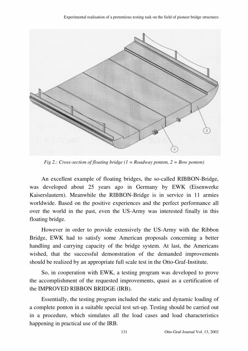
Experimental realisation of a pretentious testing task on the field of pioneer bridge structures
Fig 2.: Cross-section of floating bridge (1 = Roadway ponton, 2 = Bow ponton)
An excellent example of floating bridges, the so-called RIBBON-Bridge,
was developed about 25 years ago in Germany by EWK (Eisenwerke
Kaiserslautern). Meanwhile the RIBBON-Bridge is in service in 11 armies
worldwide. Based on the positive experiences and the perfect performance all
over the world in the past, even the US-Army was interested finally in this
floating bridge.
However in order to provide extensively the US-Army with the Ribbon
Bridge, EWK had to satisfy some American proposals concerning a better
handling and carrying capacity of the bridge system. At last, the Americans
wished, that the successful demonstration of the demanded improvements
should be realized by an appropriate full scale test in the Otto-Graf-Institute.
So, in cooperation with EWK, a testing program was developed to prove
the accomplishment of the requested improvements, quasi as a certification of
the IMPROVED RIBBON BRIDGE (IRB).
Essentially, the testing program included the static and dynamic loading of
a complete ponton in a suitable special test set-up. Testing should be carried out
in a procedure, which simulates all the load cases and load characteristics
happening in practical use of the IRB.
Otto-Graf-Journal Vol. 13, 2002 131

W. HARRE
To create that kind of most unfavourable and harmful loading situations in
the ponton means concretely to apply bending moments and longitudinal as well
as transverse loads in the same way and magnitude as it occurs, when a battle
tank MLC 70 either stands on the floating bridge or passes the bridge, like
demonstrated in the following diagram (Fig 3.).
F1
F1
F2
F F3
F F6
FF5
FF4
F
F7
F8
F9
F10
Ponton
Fig. 3: Tank loading in reality and through laboratory simulation
132

Experimental realisation of a pretentious testing task on the field of pioneer bridge structures
3. EXPERIMENTAL REALIZATION
3.1 Test set-up
There were mainly two problems to be solved:
a) Installation and program-operation of a relatively high number
(13) of hydraulic jacks with different capacities (50 kN to 2 MN)
b) Application of high bending moments (partly > 2 MNm by
means of very high horizontal forces)
Even the comparatively abundant and well assorted equipment of the
Department 2 of the Otto-Graf-Institute was not able and sufficient to solve
satisfactorily the two problems in a direct way. Especially the wanted number
and capacity of the hydraulic jacks (at least 4 jacks with more than 2 MN)
represented a considerable challenge. So, some reflection was necessary to find
a way for the experimental realization, using the available equipment.
The central idea of the solution was the consistent application of the lever-
action (Hebelgesetze): The mainly in pairs acting high horizontal forces with
opposite signs could be replaced by a lever-structure as shown basically in the
following sketch.
F12
F1-
6
F1
3
F11
Ponton
Fig. 4: Forces on the ponton
Otto-Graf-Journal Vol. 13, 2002 133

W. HARRE
F7
F8
jack > 1MN
jack > 1MN
task solutionb c
Ponton Ponton
jack < 1MN
a
Fig. 5: Solution of the testing task
Proceeding that way, several profitable effects could be achieved: the
number of the required jacks was reduced from 13 to 5, the capacity of the used
jacks could be adapted perfectly to the jacks available in the department 2 by
corresponding choice of the lever-ratios b:c and last not least – this is very
important with regard to the test set-up – the introduction of the lever structures
opens the possibility to anchor the initially horizontal forces now vertically
either in the strong floor directly or by means of test frames at hand indirectly.
The anchorage of high horizontal forces is – as experience shows – on principle
very difficult and expensive in a laboratory, because these forces have to be
turned round sooner or later to pass and anchor them finally into the floor.
After the concept of the experimental realization was found, the proceeding
was evident: after checking the available and suitable jacks in the department,
the different lever-ratios were calculated for the different loading points. After
that, all the other details were designed. Then all parts were manufactured by
EWK together with the ponton to be tested.
The following pictures will try to give an impression of the complicate and
complex test set-up:
134

Experimental realisation of a pretentious testing task on the field of pioneer bridge structures
Fig. 6. Testing arrangement on the strong floor
Otto-Graf-Journal Vol. 13, 2002 135

W. HARRE
Fig. 7.a: Mid section of testing structure
Fig. 7.b: End section of testing structure
136

Experimental realisation of a pretentious testing task on the field of pioneer bridge structures
Fig. 7.c: Oil supply system
Fig. 7.d: Complex multi-dimensional loading arrangement
Otto-Graf-Journal Vol. 13, 2002 137
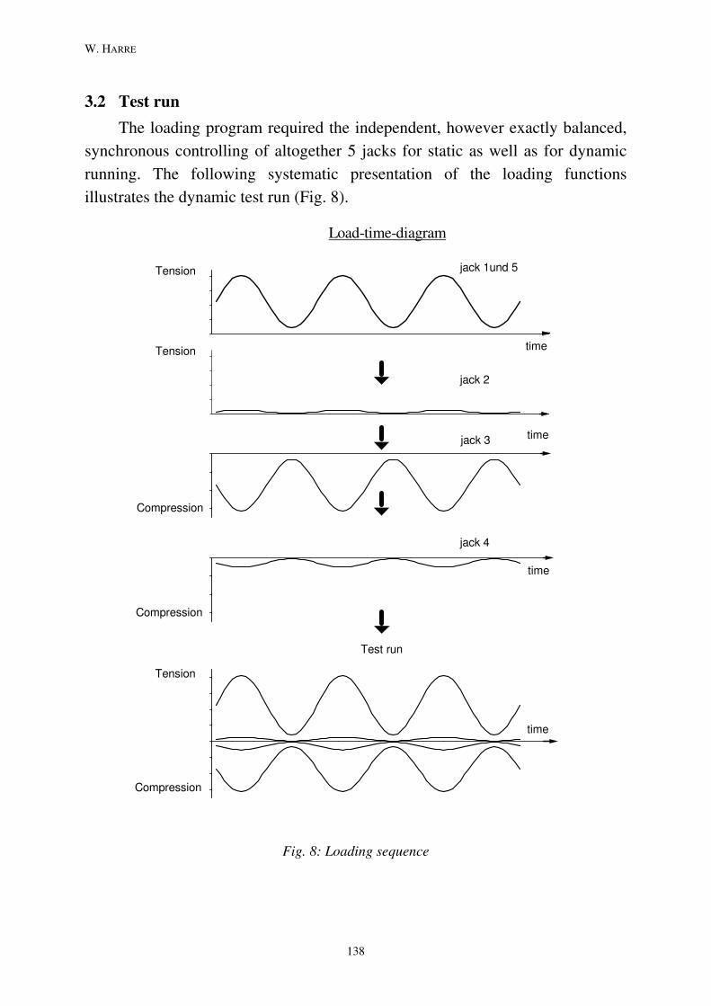
W. HARRE
3.2 Test run
The loading program required the independent, however exactly balanced,
synchronous controlling of altogether 5 jacks for static as well as for dynamic
running. The following systematic presentation of the loading functions
illustrates the dynamic test run (Fig. 8).
Test run
jack 2
jack 3
Load-time-diagram
jack 4
time
time
time
time
Compression
Tension
Compression
Compression
Tension
Tension jack 1und 5
Fig. 8: Loading sequence
138

Experimental realisation of a pretentious testing task on the field of pioneer bridge structures
The implementation of this working load test procedure supposed the
electronic coupling of the controlling units (S-59 Regler) of all the jacks.
The exact run down of the whole test program was realized by means of a
„managing“ computer, which directed the different controlling units according
to the test program. In certain intervals, that is at times after reaching
reconceived numbers of cycles, the test program also provided breaks in the
dynamic loading. During these breaks, different static extreme load
configurations were tested. All the measurements (loads, displacements, strains)
happened automatically by a multipoint measuring system. The data were stored
on CD for further evaluation. The described test set-up and equipment allowed a
dynamic loading frequency of 0.4 Hz. The estimated lifetime of the bridge was
50 000 cycles, so that the bare net time for carrying out the dynamic tests
amounted to ca. 56 hours.
The main result finally was, that the test specimen, will say the ponton
(bay), as well as the test set-up itself passed the test procedure successfully.
Apart from some insignificant cracks in the welds on uncritical structural points
of the ponton, no serious damage could be observed on the test specimen. The
test set-up also showed a perfect performance with regard to function and
reliability.
As a final statement, it can be concluded, that the experimental realization
of this pretentious testing task on the field of pioneer bridge structures was an
complete success for EWK and OGI.
Otto-Graf-Journal Vol. 13, 2002 139

W. HARRE
140
Restoration of the sarcophagus of Duke Melchior von Hatzfeld
RESTORATION OF THE SARCOPHAGUS OF DUKE MELCHIOR VON HATZFELD – THE ACCOMPANYING SCIENTIFIC AND TECHNICAL INVESTIGATIONS
SCHADENSURSACHEN DES ZERFALLS DES HATZFELD-SARKOPHAGS UND ENTWICKLUNG EINER RESTAURIERUNGSMETHODE
RESTAURATION DU SARCOPHAGE DU DUC MELCHIOR VON HATZFELD - INVESTIGATIONS SCIENTIFIQUES ET TECHNIQUES
Gabriele Grassegger
SUMMARY
The article shows the investigations that led to the cause of decay of the
alabaster sarcophagus and new methods for the restoration of the resin
impregnated piece of art. The main reason was thermal decomposition of the
gypsum and rapid rehydration accompanied by mismatching properties of the
resin. The restoration used different formulas of cold-hardening PMMA resins
combined with fillers and special coatings for 5 different steps of structural
strengthening, adhesion, gluing of cracks, reshaping and retouching. The
restoration has been successfully completed by a team of restorers.
ZUSAMMENFASSUNG
Der Alabaster-Sarkophag des Grafen von Hatzfeld (in Laudenbach) zeigte
durch problematische Restaurierungen schwere Schäden, deren Ursachen
festgestellt wurden. Die Hauptprobleme waren Wasserabspaltungen und Zerfall
des Gipses, Spannungen durch Rückhydratisierung und andere physikalische
Eigenschaften des Harzes, das zur Tränkung verwendet worden war. Es wurden
dazu passende Restaurierungsmethoden entwickelt, die auf einer 5-stufigen
Behandlung mit kalterhärtenden PMMA-Harzen beruhen. Die Behandlungen
haben die Funktionen: strukturelle Festigung, Rißverklebung, Rißverfüllung und
Antragungen, um die alte Form der Ornamente wieder herstellen zu können. Das
Verfahren ist durch ein Restauratorenteam erfolgreich umgesetzt worden und
der Sarkophag konnte wieder aufgestellt werden.
Otto-Graf-Journal Vol. 13, 2002 141
G. GRASSEGGER
RESUME
Suite à une restauration problématique, le sarcophage en albâtre du duc
Melchior von Hatzfeld avait de sévères dégradations, dont les causes furent
déterminées. Les causes principales étaient la décomposition thermique du
plâtre, les tensions mécaniques dues à une réhydratation rapide, ainsi que les
propriétés physiques mal adaptées de la résine utilisée. Nous avons développé
une nouvelle méthode de restauration basée sur un traitement en cinq phases
avec des résines PMMA durcissant à froid. Le traitement avait pour buts: le
renforcement de la structure, le colmatage des fissures et le remodelage des
ornements. La restauration a été accomplie avec succès par une équipe de
restaurateurs, le sarcophage est à nouveau exposé.
KEYWORDS: Restoration, alabaster, sarcophagus, conservation
1. INTRODUCTION
The sarcophagus of the late Duke Melchior von Hatzfeld was created in
1659 by the famous stonemason Archilles Kern from Forchtenberg
(Unterfranken). In the year 1657 Melchior von Hatzfeld had been the liberator
of Krakau against the Swedish army sent by the German Emperor. The
sarcophagus was finely carved out of a famous alabaster coming close by
Forchtenberg. It shows the Duke in a suit of armour on the cover plate and
scenes of his battles on the sides. Because of his legacy Archilles Kern created
two tombs with very similar sarcophagus one in Prausnitz (Silesia) and one in
Laudenbach (Hohenlohe) in a little chapel in the mountains, called Bergkirche
(fig. 1).
142

Restoration of the sarcophagus of Duke Melchior von Hatzfeld
Figure 1: The Hatzfeld Sarcophagus after the successful restoration and reconstruction in the Bergkirche chapel in Laudenbach (picture by Georg Schmid, restorer).
Otto-Graf-Journal Vol. 13, 2002 143
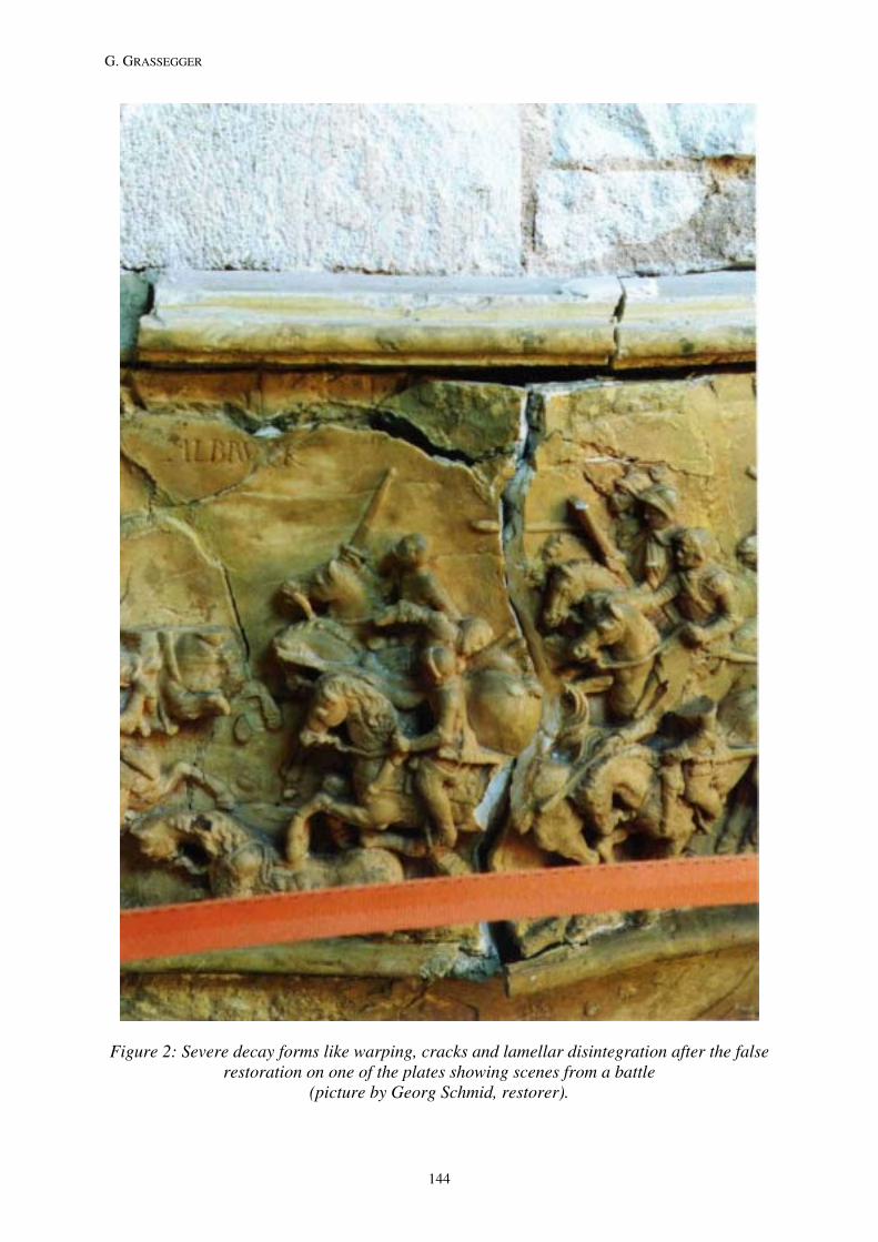
G. GRASSEGGER
Figure 2: Severe decay forms like warping, cracks and lamellar disintegration after the false restoration on one of the plates showing scenes from a battle
(picture by Georg Schmid, restorer).
144
Restoration of the sarcophagus of Duke Melchior von Hatzfeld
2. THE CAUSES OF DESTRUCTION
In 1982–1984 the object, which had been restored several times, underwent
further restoration, this time by full impregnation with acrylic resin after
preliminary tests on a sample slab had proved successful (Fig. 1 and 2).
After thorough preliminary treatment (sealing of cracks, coatings, etc.), the
process comprised the following stages: drying at up to 100°C for several days,
vacuum treatment at up to 0.2 Torr/0.9 bar, flooding with PMMA monomer
solution at up to 20 bar to saturate the object, followed by hardening at a raised
temperature, i. e. at up to 80°C.
Immediately after treatment the sarcophagus showed good superficial
strengthening but damage ranging from warping to cracking was found as early
as September 1984 after the object had been mounted on an aerated-concrete
core and replaced in the Bergkirche church. By May 1985, the damage was
more apparent. Numerous cracks had appeared and a large proportion of the
joints had opened.
In October 1986 the State Office for the Preservation of Historic
Monuments in Stuttgart (LDA B.-W.) called us in to ascertain the causes of the
damage and to try to repair it. Numerous scientific and technical tests were
performed on the object to discover the cause of damage. Our main findings
were as follows (Grassegger, 1987):
"As a result of drying and the process of impregnation with acrylic resin, the
alabaster itself had partially dehydrated into semi-hydrate and anhydrite. This
was proven in numerous surface and deep-section samples by means of phase
analysis by x-ray diffraction. The degradation behaviour of gypsum had been
underestimated because the literature often states that “plaster burning” starts
at temperatures from 120°C. (In fact, water desorps in 2 steps and this
process starts from as low as 40°C.)
"Due to its heterogeneous structure, the object was very unevenly
impregnated, which gave rise to stresses. However, 1H NMR (1H [hydrogen]
nuclear magnetic resonance spectroscopy) measurements showed that the
sarcophagus itself had been impregnated through to the centre. The PMMA
(polymethyl methacrylate synthetic resin) content in the drilling core taken
from the dog was approx. 13% PMMA by weight on the surface, falling to
Otto-Graf-Journal Vol. 13, 2002 145
G. GRASSEGGER
approx. 5% PMMA in the centre (results gained by Günther Krause, Ref. 35
FMPA).
"Examination of the alabaster under a scanning electron microscope revealed
clear coating of synthetic resin on the gypsum crystals and only very small
vacuoles and air bubbles within the resin (Figs. 3 and 4).
"Selective moistening of samples proved the existence of residual swelling
stresses in the impregnated material, leading to further warping and crack
formation. In this material, water absorption was still approx. 0.5% by
weight, whereas in a pure PMMA sample it should be 0%.
"The thermal expansion αT of the resin treated material fluctuated markedly
and unsystematically between 1.7 and 3.1 10 -5m/mK and was non-linear. Its
break point likewise fluctuated widely between + 20°C and + 80°C. The
PMMA itself was 7.3 10-5 m/mK up to a break point of + 25°C. Above that, it
was 10.5 10-5 m/mK up to 60°C. This indicates that expansion is
heterogeneous and that the expansion properties of the alabaster and the
PMMA overlap in different ways. This leads to stresses when the material is
subjected thermal strain.
"According to the αT tests and determination of the glass transition point by
differential thermoanalysis (DTA), the PMMA’s glass transition point was
approx. 60°C.
"A deep-section drilling core with an apparently even density showed very
large variations in permeability to steam. On the surface was a dense zone
with a coefficient of resistance to steam diffusion of µ = 1,200, while deeper
down the values fluctuated between µ = 380 –2,100.
After damage had occurred, due to the contact with atmospheric humidity
and in particular to the high moisture level when the sarcophagus was mounted
on an aerated concrete pedestal in the very damp church, rehydration to gypsum
was very rapid and was accompanied by stresses in line with the heterogeneity
of material as described above. This led to severe deformation and in some areas
to cracks and to disintegration of the structure in the form of expansions or
swelling of the stone texture (see fig. 2).
Hence from the scientific and technical point of view there was a most
unfortunate combination of harmful factors that could neither have been
expected nor foreseen.
146
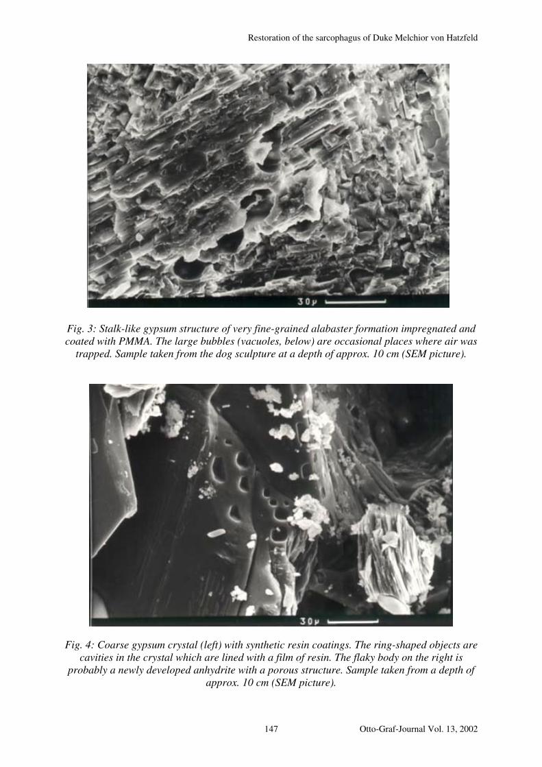
Restoration of the sarcophagus of Duke Melchior von Hatzfeld
Fig. 3: Stalk-like gypsum structure of very fine-grained alabaster formation impregnated and coated with PMMA. The large bubbles (vacuoles, below) are occasional places where air was
trapped. Sample taken from the dog sculpture at a depth of approx. 10 cm (SEM picture).
Fig. 4: Coarse gypsum crystal (left) with synthetic resin coatings. The ring-shaped objects are cavities in the crystal which are lined with a film of resin. The flaky body on the right is
probably a newly developed anhydrite with a porous structure. Sample taken from a depth of approx. 10 cm (SEM picture).
Otto-Graf-Journal Vol. 13, 2002 147
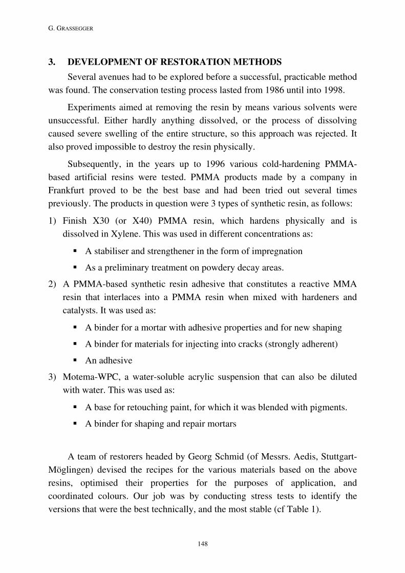
G. GRASSEGGER
3. DEVELOPMENT OF RESTORATION METHODS
Several avenues had to be explored before a successful, practicable method
was found. The conservation testing process lasted from 1986 until into 1998.
Experiments aimed at removing the resin by means various solvents were
unsuccessful. Either hardly anything dissolved, or the process of dissolving
caused severe swelling of the entire structure, so this approach was rejected. It
also proved impossible to destroy the resin physically.
Subsequently, in the years up to 1996 various cold-hardening PMMA-
based artificial resins were tested. PMMA products made by a company in
Frankfurt proved to be the best base and had been tried out several times
previously. The products in question were 3 types of synthetic resin, as follows:
1) Finish X30 (or X40) PMMA resin, which hardens physically and is
dissolved in Xylene. This was used in different concentrations as:
"A stabiliser and strengthener in the form of impregnation
"As a preliminary treatment on powdery decay areas.
2) A PMMA-based synthetic resin adhesive that constitutes a reactive MMA
resin that interlaces into a PMMA resin when mixed with hardeners and
catalysts. It was used as:
"A binder for a mortar with adhesive properties and for new shaping
"A binder for materials for injecting into cracks (strongly adherent)
"An adhesive
3) Motema-WPC, a water-soluble acrylic suspension that can also be diluted
with water. This was used as:
"A base for retouching paint, for which it was blended with pigments.
"A binder for shaping and repair mortars
A team of restorers headed by Georg Schmid (of Messrs. Aedis, Stuttgart-
Möglingen) devised the recipes for the various materials based on the above
resins, optimised their properties for the purposes of application, and
coordinated colours. Our job was by conducting stress tests to identify the
versions that were the best technically, and the most stable (cf Table 1).
148

Restoration of the sarcophagus of Duke Melchior von Hatzfeld
Table 1: Composition of the restoration materials employed (Restoration expert Georg Schmid and team, Möglingen).
Application Description/Recipe
Adhesive mortar, fine formula for repair and shaping
FM1= Acrylic resin suspension (Motema WPC) binder blended with Lenzin (natural gypsum) filler to a stiff, doughy consistency.
Injection mortar for adhesive and bridging of the cracks
I2= 1 part*) resin (Motema injection PMMA 220) + 1% by weight (in relation to the resin) peroxide catalyst plus 2 parts glass pellets <50µ.
Structural strengthening of the damaged alabaster regions and pre-treatment of sides of cracks
Impregnation with 5% PMMA solution Finish X40 (further diluted with Xylol to 5% resin content, results cf. Table 2).
Intermediate treatment (intermediate varnish) Impregnation with Finish X40, diluted to 5% resin content with ethyl acetate (to prevent previously applied coatings from dissolution.)
Final treatment, retouching paint. R1 = Retouching of repair mortars (pigments and Motema-WPC binder, i. e. water polymer coating, Pigments: Mixol: ground, natural standard pigment mixtures).
*) = parts by weight
Preliminary testing of the resins to establish their suitability
The synthetic resins were investigated in several tests to establish their
suitability and durability. This included artificial ageing simulations, tests to
establish their penetration into the alabaster – which in cracks included
measuring adhesion and determining their strengthening effect. All this was
done using various recipes. Here we show, by way of example, only the increase
in resistance to pressure, and adhesion (Tables 2 and 3).
Strengthening the alabaster
Strengthening was required because some of the alabaster had become
powdery in defective parts and on the surface. Powdery layers along the sides of
some cracks also needed to be stabilised before sealing. The gypsum was fully
impregnated, to saturation point in the case of samples 1 to 6, with solvents and
with Finish X 40 methacrylate solution to strengthen the structure. For
comparison, untreated, freshly quarried alabaster material (samples A–C) was
measured at the same time (Table 1).
Otto-Graf-Journal Vol. 13, 2002 149
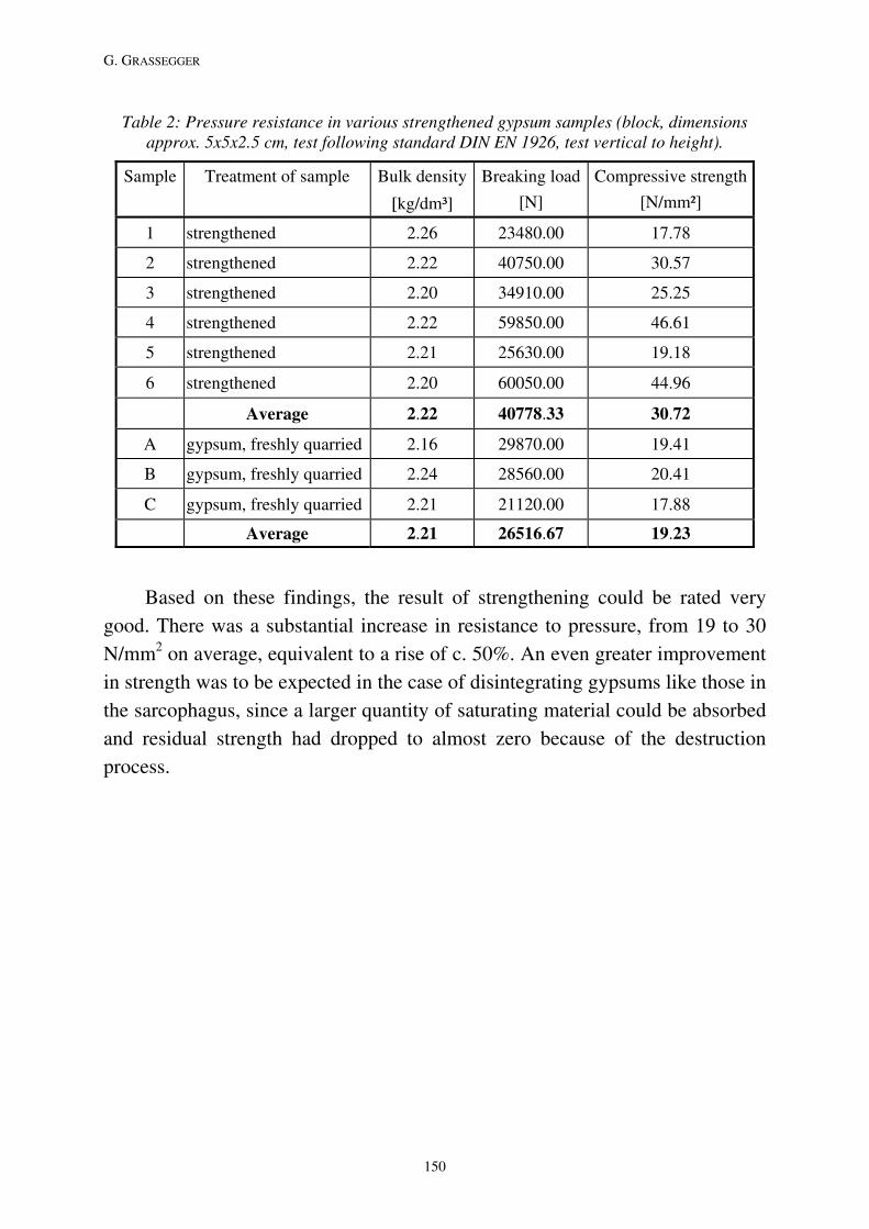
G. GRASSEGGER
Table 2: Pressure resistance in various strengthened gypsum samples (block, dimensions approx. 5x5x2.5 cm, test following standard DIN EN 1926, test vertical to height).
Sample Treatment of sample Bulk density
[kg/dm³]
Breaking load
[N]
Compressive strength
[N/mm²]
1 strengthened 2.26 23480.00 17.78
2 strengthened 2.22 40750.00 30.57
3 strengthened 2.20 34910.00 25.25
4 strengthened 2.22 59850.00 46.61
5 strengthened 2.21 25630.00 19.18
6 strengthened 2.20 60050.00 44.96
Average 2.22 40778.33 30.72
A gypsum, freshly quarried 2.16 29870.00 19.41
B gypsum, freshly quarried 2.24 28560.00 20.41
C gypsum, freshly quarried 2.21 21120.00 17.88
Average 2.21 26516.67 19.23
Based on these findings, the result of strengthening could be rated very
good. There was a substantial increase in resistance to pressure, from 19 to 30
N/mm2 on average, equivalent to a rise of c. 50%. An even greater improvement
in strength was to be expected in the case of disintegrating gypsums like those in
the sarcophagus, since a larger quantity of saturating material could be absorbed
and residual strength had dropped to almost zero because of the destruction
process.
150
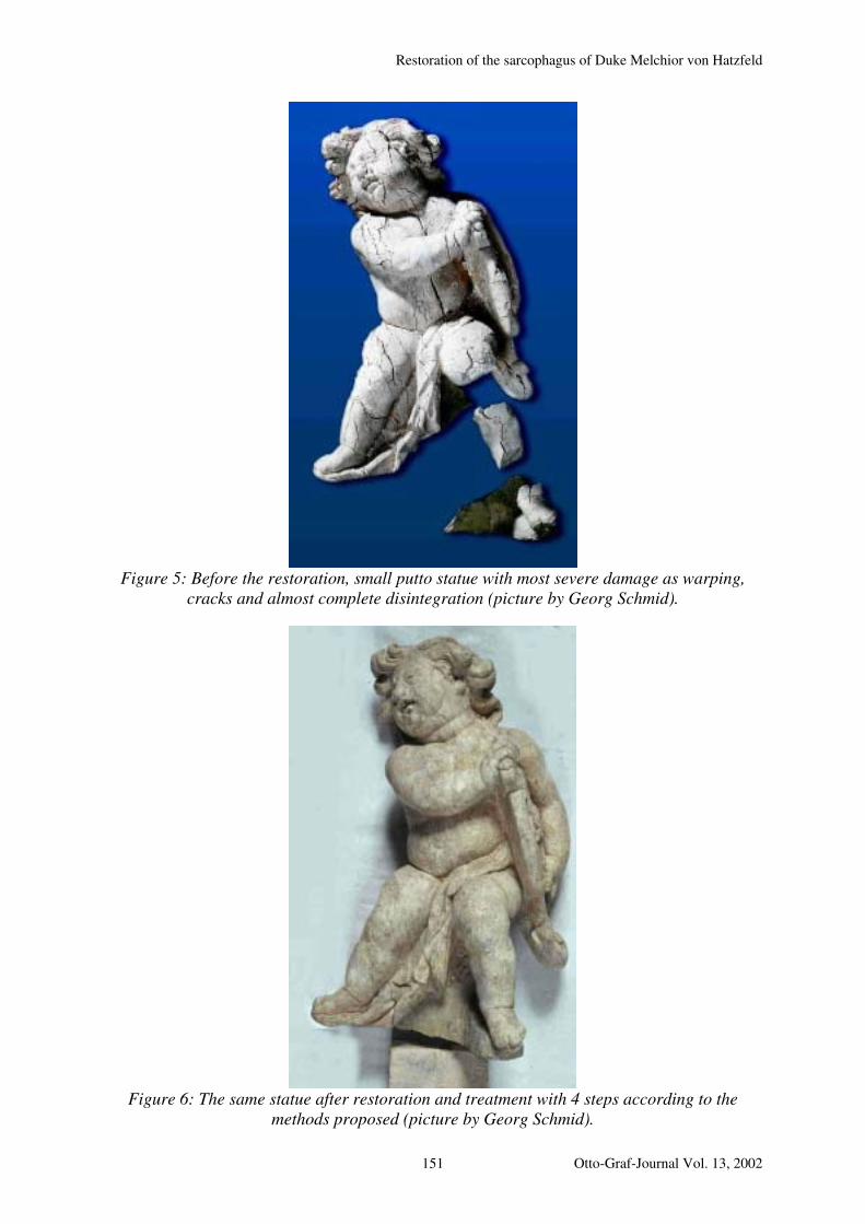
Restoration of the sarcophagus of Duke Melchior von Hatzfeld
Figure 5: Before the restoration, small putto statue with most severe damage as warping,
cracks and almost complete disintegration (picture by Georg Schmid).
Figure 6: The same statue after restoration and treatment with 4 steps according to the
methods proposed (picture by Georg Schmid).
Otto-Graf-Journal Vol. 13, 2002 151
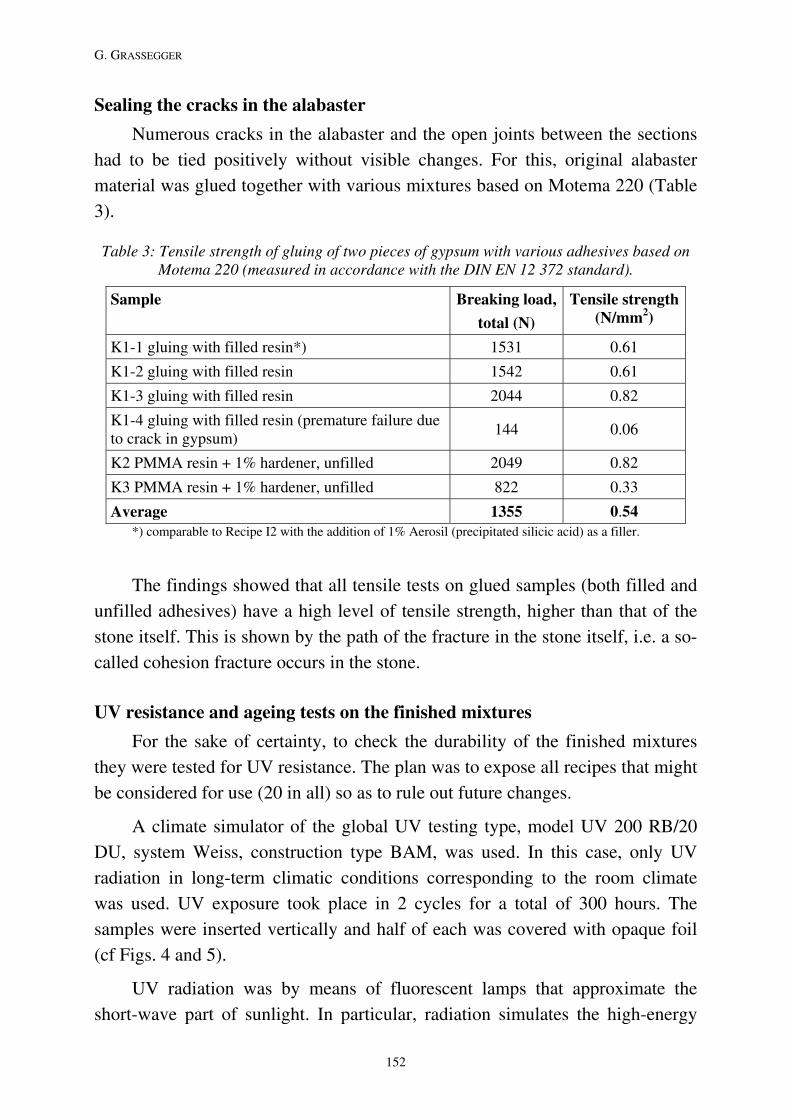
G. GRASSEGGER
Sealing the cracks in the alabaster
Numerous cracks in the alabaster and the open joints between the sections
had to be tied positively without visible changes. For this, original alabaster
material was glued together with various mixtures based on Motema 220 (Table
3).
Table 3: Tensile strength of gluing of two pieces of gypsum with various adhesives based on Motema 220 (measured in accordance with the DIN EN 12 372 standard).
Sample Breaking load,
total (N)
Tensile strength (N/mm2)
K1-1 gluing with filled resin*) 1531 0.61
K1-2 gluing with filled resin 1542 0.61
K1-3 gluing with filled resin 2044 0.82
K1-4 gluing with filled resin (premature failure due to crack in gypsum)
144 0.06
K2 PMMA resin + 1% hardener, unfilled 2049 0.82
K3 PMMA resin + 1% hardener, unfilled 822 0.33
Average 1355 0.54 *) comparable to Recipe I2 with the addition of 1% Aerosil (precipitated silicic acid) as a filler.
The findings showed that all tensile tests on glued samples (both filled and
unfilled adhesives) have a high level of tensile strength, higher than that of the
stone itself. This is shown by the path of the fracture in the stone itself, i.e. a so-
called cohesion fracture occurs in the stone.
UV resistance and ageing tests on the finished mixtures
For the sake of certainty, to check the durability of the finished mixtures
they were tested for UV resistance. The plan was to expose all recipes that might
be considered for use (20 in all) so as to rule out future changes.
A climate simulator of the global UV testing type, model UV 200 RB/20
DU, system Weiss, construction type BAM, was used. In this case, only UV
radiation in long-term climatic conditions corresponding to the room climate
was used. UV exposure took place in 2 cycles for a total of 300 hours. The
samples were inserted vertically and half of each was covered with opaque foil
(cf Figs. 4 and 5).
UV radiation was by means of fluorescent lamps that approximate the
short-wave part of sunlight. In particular, radiation simulates the high-energy
152

Restoration of the sarcophagus of Duke Melchior von Hatzfeld
UV-A and UV-B rays (λ = 300–420 nm) that could trigger photo-oxidation. The
combination of fluorescent lamps employed corresponded to the spectral
distribution as per Method B of DIN 53 384 E.
Results of UV ageing
No kind of UV ageing or other damage was found to result from storage in
the room climate conditions and UV radiation. In this respect, the restoration
materials must be described as durable and stable.
CONCLUDING REMARKS
These extensive tests created excellent conditions for the tomb’s lasting
restoration. Skilful implementation by the team of restorers led by t Mr. Georg
Schmid/Stuttgart Möglingen reinstated the tomb to its former beauty (see Fig. 1
and 5).
By way of additional protection, the grave chapel containing the
sarcophagus is to be air-conditioned with the aim of avoiding alternating strains
in future. For the reasons stated at the beginning, a constant climate of approx.
10°C and a maximum of 50% relative humidity is to be aimed for.
ACKNOWLEDGEMENT
Thanks to the whole group of people who participated for the long period
of investigations and trials until the sarcophagus could be restored, especially to
Mr. Otto Wölbert and Mr. Meckes from the LDA who were the driving force of
the project and never gave up.
The whole history of the piece of art and it’s restoration will be published
in the upcoming issue of the “Nachrichtenblatt der Denkmalpflege in Baden-
Württemberg”, 4/2002 by a team of authors Otto Wölbert (restoration history),
Georg Schmid (restoration), Judith Breuer (art history), Robert Vix
(Architecture) and Gabriele Grassegger (technical investigations).
REFERENCES/INTERNAL REPORTS (SELECTION)
Grassegger, G. (1987): Hatzfeld-Grabmal, Bergkirche Laudenbach -
Untersuchung zur Schadensursache an einem Alabaster-Sarkophag nach einer
Kunstharz-Volltränkung, Nr. D3 140 008/GR (LDA internal report dated
18.9.1987)
Otto-Graf-Journal Vol. 13, 2002 153

G. GRASSEGGER
Grassegger, G. (2001): Restaurierung des Hatzfeld-Grabmals, Mechanische
Untersuchung von Festigungen und Probeklebungen auf Alabastergips“, Nr.
32-804073 (internal report of the Otto Graf Institute, Research and Testing
Establishment for Building and Construction [FMPA] dated 2.7.2001)
Grassegger, G. (2002): Restaurierung des Hatzfeld-Grabmals – Test der UV-
Alterungsbeständigkeit bei den fertigen Restaurierungsmateralien (Kittmörtel,
Klebungen, Injektagen und Retouchen), Berichtsnummer: 32 804 073 000-2
(FMPA internal report dated 3.5.2002).
154
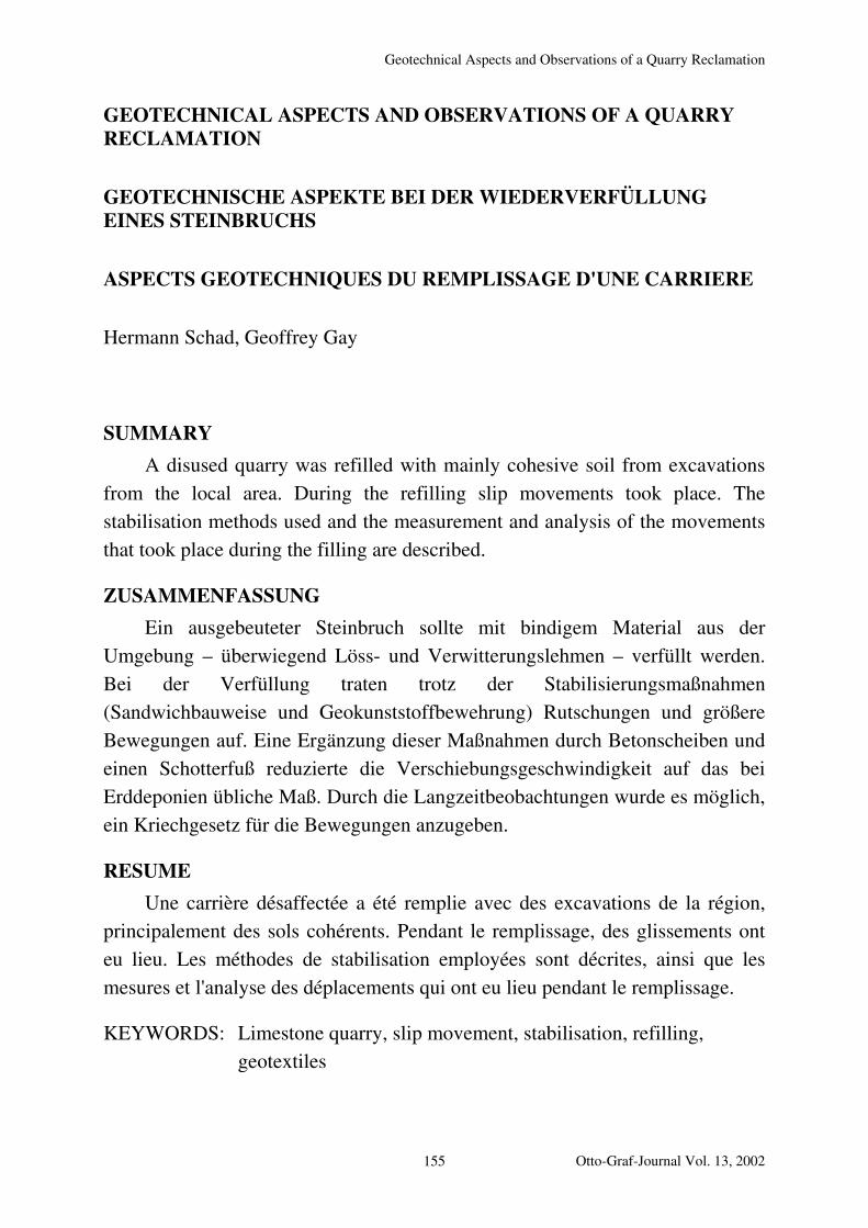
Geotechnical Aspects and Observations of a Quarry Reclamation
GEOTECHNICAL ASPECTS AND OBSERVATIONS OF A QUARRY RECLAMATION
GEOTECHNISCHE ASPEKTE BEI DER WIEDERVERFÜLLUNG EINES STEINBRUCHS
ASPECTS GEOTECHNIQUES DU REMPLISSAGE D'UNE CARRIERE
Hermann Schad, Geoffrey Gay
SUMMARY
A disused quarry was refilled with mainly cohesive soil from excavations
from the local area. During the refilling slip movements took place. The
stabilisation methods used and the measurement and analysis of the movements
that took place during the filling are described.
ZUSAMMENFASSUNG
Ein ausgebeuteter Steinbruch sollte mit bindigem Material aus der
Umgebung – überwiegend Löss- und Verwitterungslehmen – verfüllt werden.
Bei der Verfüllung traten trotz der Stabilisierungsmaßnahmen
(Sandwichbauweise und Geokunststoffbewehrung) Rutschungen und größere
Bewegungen auf. Eine Ergänzung dieser Maßnahmen durch Betonscheiben und
einen Schotterfuß reduzierte die Verschiebungsgeschwindigkeit auf das bei
Erddeponien übliche Maß. Durch die Langzeitbeobachtungen wurde es möglich,
ein Kriechgesetz für die Bewegungen anzugeben.
RESUME
Une carrière désaffectée a été remplie avec des excavations de la région,
principalement des sols cohérents. Pendant le remplissage, des glissements ont
eu lieu. Les méthodes de stabilisation employées sont décrites, ainsi que les
mesures et l'analyse des déplacements qui ont eu lieu pendant le remplissage.
KEYWORDS: Limestone quarry, slip movement, stabilisation, refilling,
geotextiles
Otto-Graf-Journal Vol. 13, 2002 155
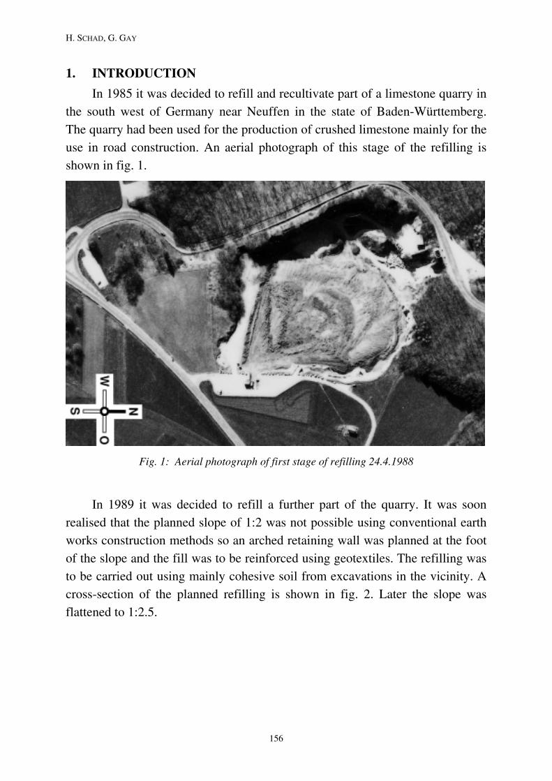
H. SCHAD, G. GAY
1. INTRODUCTION
In 1985 it was decided to refill and recultivate part of a limestone quarry in
the south west of Germany near Neuffen in the state of Baden-Württemberg.
The quarry had been used for the production of crushed limestone mainly for the
use in road construction. An aerial photograph of this stage of the refilling is
shown in fig. 1.
Fig. 1: Aerial photograph of first stage of refilling 24.4.1988
In 1989 it was decided to refill a further part of the quarry. It was soon
realised that the planned slope of 1:2 was not possible using conventional earth
works construction methods so an arched retaining wall was planned at the foot
of the slope and the fill was to be reinforced using geotextiles. The refilling was
to be carried out using mainly cohesive soil from excavations in the vicinity. A
cross-section of the planned refilling is shown in fig. 2. Later the slope was
flattened to 1:2.5.
156

Geotechnical Aspects and Observations of a Quarry Reclamation
Fig. 2: Cross-section of second stage of the refilling 1990
2 SLIP MOVEMENTS AND STABILISATION
In November 1997 it was noticed that relatively large slip movements must
have taken place because a natural stone wall surrounding a manhole had been
deformed considerably. (see fig. 3). The refilling was not complete at this time.
Fig. 3: Deformed natural stone wall
Otto-Graf-Journal Vol. 13, 2002 157

H. SCHAD, G. GAY
It was therefore decided to set up a grid of measuring points to observe the
movements of the slope. The grid points are shown in fig. 4.
Fig. 4: Plan of grid points used between 24.11.97 and 21.11.00
The first measurement took place in November 1997. After the first two
measurements with a weeks difference between them it appeared that the
deformation rate was slowing down. It had reduced from 9mm/d to 5mm/d. In
the third week however the speed increased to 20mm/d so it was decided to
increase the factor of safety by stabilising the foot of the slope using concrete
buttresses with crushed rock between them as shown in figs. 5 and 6.
158
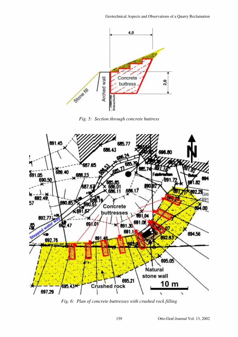
Geotechnical Aspects and Observations of a Quarry Reclamation
Fig. 5: Section through concrete buttress
Fig. 6: Plan of concrete buttresses with crushed rock filling
Otto-Graf-Journal Vol. 13, 2002 159
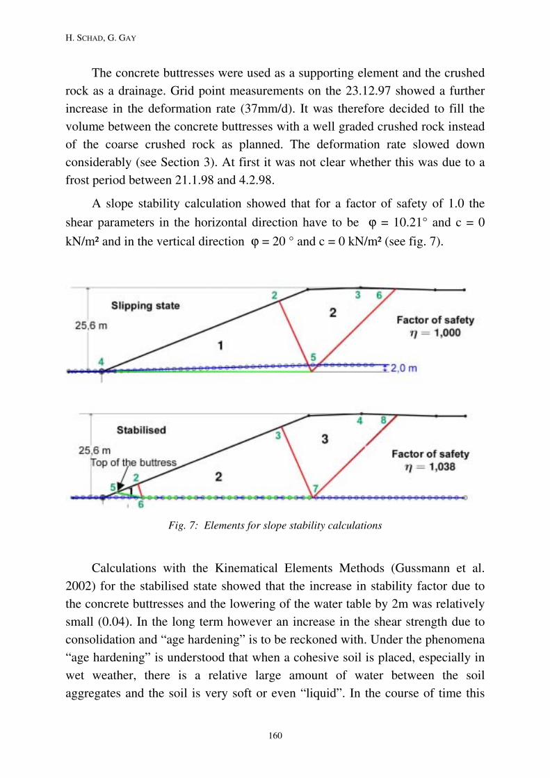
H. SCHAD, G. GAY
The concrete buttresses were used as a supporting element and the crushed
rock as a drainage. Grid point measurements on the 23.12.97 showed a further
increase in the deformation rate (37mm/d). It was therefore decided to fill the
volume between the concrete buttresses with a well graded crushed rock instead
of the coarse crushed rock as planned. The deformation rate slowed down
considerably (see Section 3). At first it was not clear whether this was due to a
frost period between 21.1.98 and 4.2.98.
A slope stability calculation showed that for a factor of safety of 1.0 the
shear parameters in the horizontal direction have to be ϕ = 10.21° and c = 0
kN/m² and in the vertical direction ϕ = 20 ° and c = 0 kN/m² (see fig. 7).
Fig. 7: Elements for slope stability calculations
Calculations with the Kinematical Elements Methods (Gussmann et al.
2002) for the stabilised state showed that the increase in stability factor due to
the concrete buttresses and the lowering of the water table by 2m was relatively
small (0.04). In the long term however an increase in the shear strength due to
consolidation and “age hardening” is to be reckoned with. Under the phenomena
“age hardening” is understood that when a cohesive soil is placed, especially in
wet weather, there is a relative large amount of water between the soil
aggregates and the soil is very soft or even “liquid”. In the course of time this
160
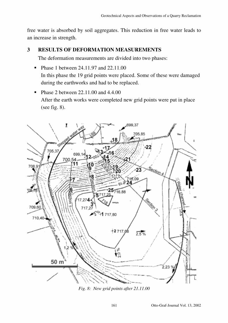
Geotechnical Aspects and Observations of a Quarry Reclamation
free water is absorbed by soil aggregates. This reduction in free water leads to
an increase in strength.
3 RESULTS OF DEFORMATION MEASUREMENTS
The deformation measurements are divided into two phases:
"Phase 1 between 24.11.97 and 22.11.00
In this phase the 19 grid points were placed. Some of these were damaged
during the earthworks and had to be replaced.
"Phase 2 between 22.11.00 and 4.4.00
After the earth works were completed new grid points were put in place
(see fig. 8).
Fig. 8: New grid points after 21.11.00
Otto-Graf-Journal Vol. 13, 2002 161

H. SCHAD, G. GAY
The decisive deformation kinematics as derived from the deformation
measurements between 24.11.97 and 8.2.98 are shown in fig. 4. It can be seen
that the part which is reinforced with geotextiles moved horizontally as a block.
The displacement rates of the points 16 and 17 (fig. 4) are characteristic for
the lower part of the slope. The average deformations and the resulting
deformation rates are shown in the following diagram.
Fig. 9: Displacements of the lower part during the first 72 days
After construction was completed a horizontal deformation of 16mm in the
course of 1.5 years was measured at grid point 5 (see fig. 8). The vertical
deformations of this point during the same time interval were 36mm. The
maximum settlement measured on the “plateau” was 48mm. At the foot of the
slope the maximum deformations at grid point 10 were horizontal 14mm and
vertical 3mm. Of special note is the similarity of the settlements of the grid
points 1 to 5 on the “plateau”. Inside 1.5 years (21.11.00 to 4.4.02) they were
40mm, 48mm, 39mm, 36mm and 35mm as shown in fig. 10.
162
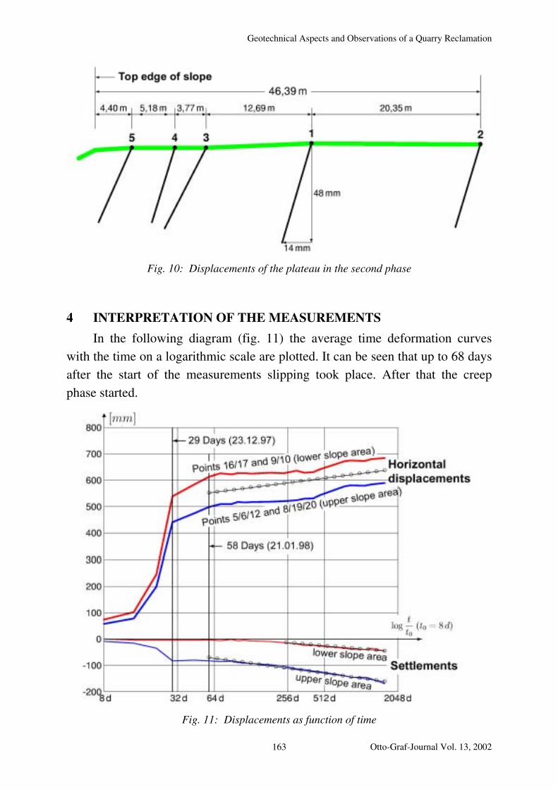
Geotechnical Aspects and Observations of a Quarry Reclamation
Fig. 10: Displacements of the plateau in the second phase
4 INTERPRETATION OF THE MEASUREMENTS
In the following diagram (fig. 11) the average time deformation curves
with the time on a logarithmic scale are plotted. It can be seen that up to 68 days
after the start of the measurements slipping took place. After that the creep
phase started.
Fig. 11: Displacements as function of time
Otto-Graf-Journal Vol. 13, 2002 163
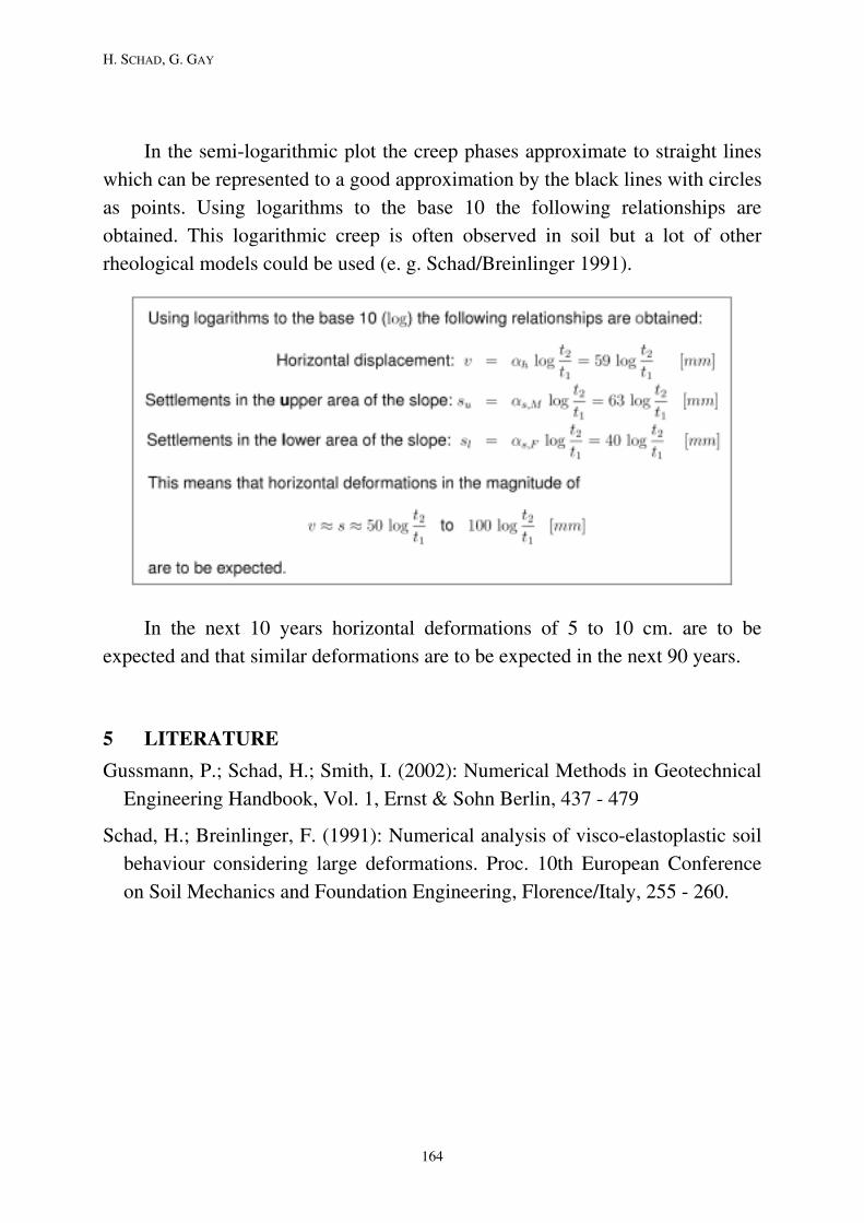
H. SCHAD, G. GAY
In the semi-logarithmic plot the creep phases approximate to straight lines
which can be represented to a good approximation by the black lines with circles
as points. Using logarithms to the base 10 the following relationships are
obtained. This logarithmic creep is often observed in soil but a lot of other
rheological models could be used (e. g. Schad/Breinlinger 1991).
In the next 10 years horizontal deformations of 5 to 10 cm. are to be
expected and that similar deformations are to be expected in the next 90 years.
5 LITERATURE
Gussmann, P.; Schad, H.; Smith, I. (2002): Numerical Methods in Geotechnical
Engineering Handbook, Vol. 1, Ernst & Sohn Berlin, 437 - 479
Schad, H.; Breinlinger, F. (1991): Numerical analysis of visco-elastoplastic soil
behaviour considering large deformations. Proc. 10th European Conference
on Soil Mechanics and Foundation Engineering, Florence/Italy, 255 - 260.
164
Non-destructive detection of longitudinal cracks in glulam beams
NON-DESTRUCTIVE DETECTION OF LONGITUDINAL CRACKS IN GLULAM BEAMS
ZERSTÖRUNGSFREIE MESSUNG VON LÄNGSRISSEN IN BRETTSCHICHTHOLZ-TRÄGERN
DÉTECTION NON DESTRUCTIVE DES FISSURES LONGITUDINALES DANS LES POUTRES DE BOIS LAMELLÉ COLLÉ
Simon Aicher, Gerhard Dill-Langer, Thomas Ringger
SUMMARY
The paper reports on the detection and length characterisation of
longitudinal cracks in glued laminated timber (glulam) beams by means of
ultrasound (US) pulse transmission method. In the preliminary study one large
glulam beam with a crack starting at one end-grain face and ending at about one
third of total beam length has been evaluated. For the transmission
measurements US pulses have been applied to the narrow faces of the beam,
thus propagating parallel to cross-sectional depth perpendicular to fibre. The
beam has been scanned by a transmitter / receiver pair of US transducers shifted
along the longitudinal beam axis. The recorded full US wave signals were
evaluated for three different scalar parameters being “time of flight”, “peak-to-
peak amplitude” and “first amplitude”. The comparison of the visual inspection
with the US parameters, showing significantly different scatter ranges, yielded a
satisfactory agreement with respect to the determination of crack length. The
NDT crack detection based on the parameter “time of flight” was also
satisfactory when the crack extended only over a part of the beam width, i. e. not
being visually detectable from one of both side faces. The latter can be very
important for in-situ inspection of beams in buildings with assumed or partial
cracks.
Otto-Graf-Journal Vol. 13, 2002 165

S. AICHER, G. DILL-LANGER, T. RINGGER
ZUSAMMENFASSUNG
Der Aufsatz berichtet über den Nachweis und die Längenmessung von
longitudinalen Rissen in Brettschichtholz (BSH) -Trägern mittels der Methode
der Durchschallung mit Ultraschallpulsen. In der orientierenden Studie wurde
ein großer Brettschichtholzträger mit einem Riss untersucht, wobei der Riss von
einer Hirnholzfläche ausging und innerhalb des ersten Drittels der Trägerlänge
endete. Für die Transmissionsmessungen wurden Ultraschallpulse auf die
Schmalseiten der Träger aufgebracht, so dass diese sich parallel zur
Querschnittshöhe und damit rechtwinklig zur Faserrichtung ausbreiteten. Der
Träger wurde mit einem Ultraschall Geber / Empfänger-Paar in Richtung der
Trägerachse abgerastert. Die aufgezeichneten vollständigen Ultraschallsignale
wurden hinsichtlich dreier verschiedener skalarer Parameter ausgewertet:
Signal-Laufzeit, Signalstärke und erste Amplitude. Der Vergleich der visuellen
Charakterisierung mit den Ultraschallparametern, die jeweils deutlich
unterschiedliche Streubreiten aufwiesen, ergab eine zufriedenstellende
Übereinstimmung hinsichtlich der Bestimmung der Risslänge. Die
zerstörungsfreie Risserkennung auf Grundlage des Parameters "Signal-Laufzeit"
war auch dort noch zufriedenstellend, wo sich der Riss nur über einen Teil der
Querschnittsbreite erstreckte, also auf einer der beiden Seitenflächen schon nicht
mehr sichtbar war. Letzteres kann für die in-situ Beurteilung von Trägern in
realen Bauwerken mit vermuteten oder teilweise vorhandenen Rissen sehr
wichtig sein.
RÉSUMÉ
L’article traite de la détection et de la caractérisation des fissures
longitudinales dans les poutres en bois lamellé collé, au moyen d’une méthode
de transmission des impulsions ultrasons. Lors de travaux préliminaires, une
poutre présentant une fissure commençant à l’une des extrémités et s’étendant
jusqu’au tiers de la longueur totale a été étudiée. Les impulsions d’ultrasons sont
appliquées sur les deux faces les plus étroites de la poutre et se propagent
parallèlement à sa section, c’est à dire perpendiculairement aux fibres du bois.
Les capteurs ultrasons (émetteur et transmetteur) balaient alors la poutre suivant
son axe longitudinal. Le signal enregistré fournit trois paramètres différents: le
temps de propagation du signal, son amplitude pic à pic et sa première
amplitude. La comparaison entre les indications obtenues par la méthode des
166
Non-destructive detection of longitudinal cracks in glulam beams
ultrasons et l’évaluation visuelle sont en accord quant à la détermination de la
longueur de la fissure. La détection basée sur le seul paramètre « durée de
propagation » est également satisfaisante lorsque la fissure ne s’étend que sur
une partie de l’épaisseur, c’est à dire lorsqu’elle ne traverse pas la poutre de part
en part. Ce dernier cas est très intéressant pour l’inspection in-situ des
constructions présentant des fissures ou des risques de fissure.
KEYWORDS: non-destructive testing, ultrasound, pulse transmission, crack in
glulam beams, scalar ultrasound parameters
1. INTRODUCTION
Non-destructive evaluation of the state of integrity resp. of defects or
partial damages in structural building elements generally represents an important
issue. The capability of NDT based reliable assessment of components enhances
the acceptance of building systems or materials, may affect safety factors and
enables assessment of upgrading or rehabilitation works. Timber and glulam
beams despite all positive aspects are prone to longitudinal cracks generally
resulting from interaction of poor constructive detailing and unaccounted
climatic stresses. Longitudinal cracks primarily occur at i) support areas due to
interaction of shear stresses and climate and ii) at notches, holes and in apex
areas of curved / tapered beams due to tension stresses perpendicular to grain
bound to undue load actions and / or often climate stresses. Finally,
iii) longitudinal cracks can occur from poor glue lines generally bound to
trespass of open / closed curing times of the adhesives.
The reliable assessment of the extent of damage and of the result of the
repair works represent the two equally important aspects of the NDT assessment
of damaged or upgraded construction elements. In many cases a visual
inspection of the beams is very costly or almost impossible. Today reliable NDT
tools for employment in the sketched area are missing for lumber / glulam
beams being contrary to constructions with some other important building
materials. The reason for this NDT lag consists i.a. in the anisotropy,
inhomogeneity and the high damping characteristics of the natural material
wood.
Otto-Graf-Journal Vol. 13, 2002 167

S. AICHER, G. DILL-LANGER, T. RINGGER
Timber Department of Otto-Graf-Institute being deeply involved in the
assessment / expertises of damages, repair proposals and technical approval of
rehabilitation works has started to focus on active NDT methods about a year
ago. This paper gives some preliminary results of one of the on-going projects.
It is reported on the detection and length characterisation of longitudinal cracks
in glued laminated timber (glulam) by means of ultrasound (US) pulse
transmission method. The US method has been chosen due to its sensitivity to
impedance changes at discrete boundaries. Former literature known attempts in
this field [KLINGSCH, 1991; KIMURA ET AL 1991] dealt with artificial defects,
being rather thick saw cuts of defined length parallel to beam axis and over full
cross-sectional width. The results and the practical relevance of the exclusive
focus on such slots / cracks has been discussed controversially in the involved
engineering community. In the investigation reported here a fully practice
relevant crack resp. cracked beam was investigated.
2. EXPERIMENTAL SET-UP
The investigated specimen represented a part cut from a large beam with a
round hole loaded until failure in bending, compare Fig. 1a. The beam had failed
with two large cracks initiated at the hole periphery by high local stresses
perpendicular to grain. The crack propagation was then driven by both, shear
and tension stresses perpendicular to grain.
The investigated NDT specimen (Fig. 1b) showed an open crack over full
width b at end grain face Y closer to the former hole location and no visible
crack at the opposite end grain face Z. Thus, despite disputable accuracy of
visual inspection the crack must end within the specimen as the latter consisted
of one massive piece.
168

Non-destructive detection of longitudinal cracks in glulam beams
a)
l = 2100
p/2 p/2
Lc
h = 440
T
B
Y
Z
cracks atultimate load
900
120
investigatedNDT specimen
originallyted beamtes
b)
l = 2100
b = 120
h =
44
0
Top narrow face (T)
Bottom narrow face (B)
visible part of the crack
end grainface Y
end grainface Z
"right" wide face II
10
0
33
33
xy
Fig. 1a,b: Original location and dimensions of the employed NDT specimen. a) larger cracked beam from which the NDT specimen was cut out after failure of the beam b) view and dimensions of partially cracked NDT specimen
Otto-Graf-Journal Vol. 13, 2002 169

S. AICHER, G. DILL-LANGER, T. RINGGER
The dimensions of the block were (width b × depth h × length l): 120 mm ×
440 mm × 2100 mm. Starting at end-grain face Y and proceeding in the
longitudinal (x-) beam direction, the crack is visible at both side-faces I and II
for the major part of the crack length (compare chap. 4).
The ultrasonic NDT evaluation / assessment of the crack (length) was
throughout performed by means of a pair of piezoelectric (US) transducers.
Transmitter and receiver were positioned oppositely at mid-width of the narrow
faces T and B of the beam specimen and aligned parallel to depth. Starting at the
end-grain face Y with the opened crack the transducer pair was moved along
beam length l with increments of
x = 50 mm towards the end grain face Z. At
each position an ultrasonic pulse synthesized by a generator unit was put to the
specimen by the piezoelectric transmitter. Figure 2 shows a schematic
representation of the experimental set-up. The fixation of the transmitter and of
the receiver differed. The transmitter was throughout fixed to the surface by a
hot melt adhesive also serving as coupling agent. Contrary, the receiver was not
glued to but applied to the surface by hand pressure without using any kind of
coupling agent.
At each location x a number of 25 repetitive measurements were performed
in order to enable noise reduction. As the crack was not centred in the middle of
the cross-sectional depth but much closer (~70 mm) to narrow face B it was
questioned whether there might be an influence if the transmitter is at a closer or
more remote distance to the crack. Therefore two test series S1 and S2 were
performed with the transmitter first being at narrow side T and then at narrow
side B.
170
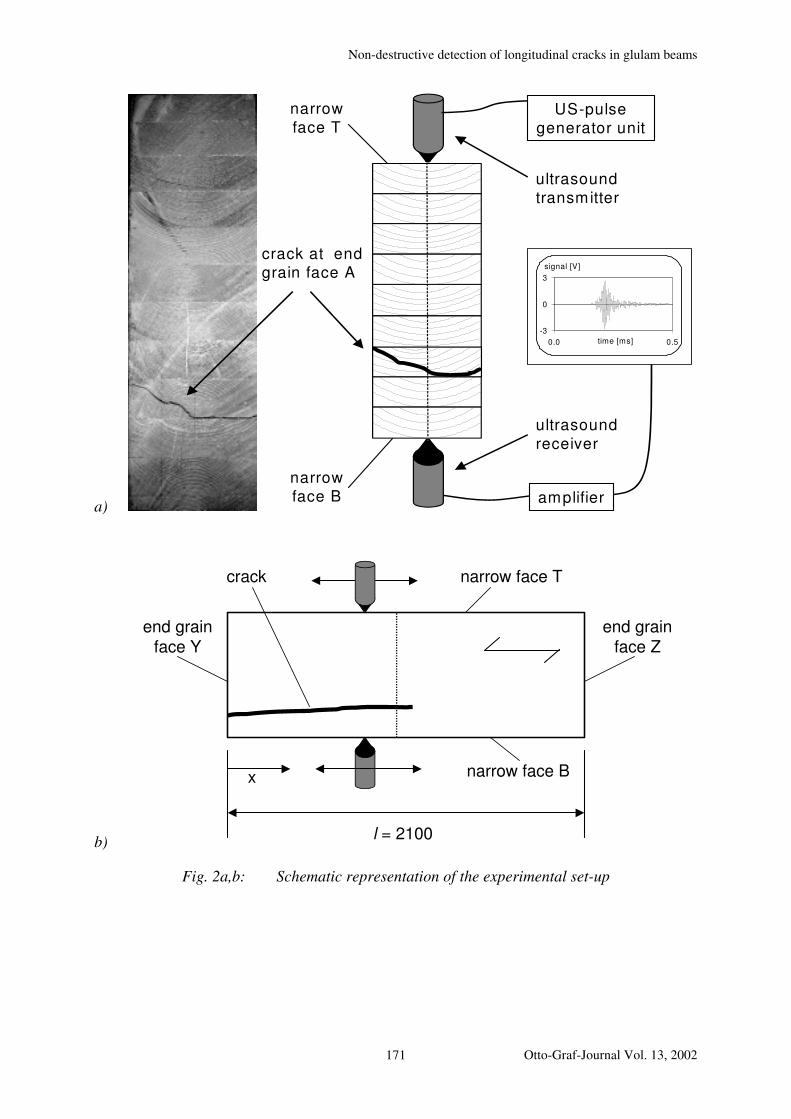
Non-destructive detection of longitudinal cracks in glulam beams
a)
crack at endgrain face A
ultrasoundtransmitter
ultrasoundreceiver
US-pulsegenerator unit
amplifier
narrowface T
narrowface B
-3
0
3
0.0 0.5time [ms]
signal [V]
b)
narrow face T
end grainface Z
narrow face B
end grainface Y
crack
x
l = 2100
Fig. 2a,b: Schematic representation of the experimental set-up
Otto-Graf-Journal Vol. 13, 2002 171
S. AICHER, G. DILL-LANGER, T. RINGGER
3. NDT EQUIPMENT
The generator unit (USG 20, Geotron Electronics), originally optimised for
NDT of concrete, produced high voltage pulses with main frequencies between
20 kHz and 350 kHz. The duration of a single pulse was less than 1 ms.
The ultrasonic transducers (UPG-D 3037, UPE-D 3038, Geotron
Electronics) used in the experiments were piezoelectric converters with a
coupling-surface of 3 mm in diameter. The transducers showed a multi-resonant
frequency characteristic with main peak values between 20 and 100 kHz.
The received ultrasonic pulses have been amplified by a broadband
amplifier (AM 502, Tektronix) with an amplification factor of 100 dB. The
complete signals were recorded by a PC based transient recorder with 12 bit
amplitude resolution and 20 MHz time resolution.
4. VISUAL CHARACTERIZATION OF THE CRACK DIMENSIONS
For correlation of the ultrasound NDT parameters with the length of the
crack in longitudinal beam direction and with the crack opening, the dimensions
of the crack were determined by visual inspection at both wide side faces I and
II of the specimen. The crack openings were measured with a feeler gauge.
Figures 3 a and 3 c give a schematic illustration of shape, position and
dimensions of the crack according to the visual characterization and feeler gauge
measurements at the two wide faces I and II, while Fig. 3 b shows a top view
indicating the projected crack area. According to the visual findings the crack
can be divided into three different sections.
In section A (0 ≤ x ≤ 53 cm), the crack is characterized by measurable
openings of 1.2 mm (x = 0) to 0.4 mm (x = 53 cm) at side face I; at side face II
the respective dimensions are: 0.4 mm (x = 0) to 0.05 mm (x = 53 cm).
In section B (53 cm < x ≤ 67 cm) a crack-opening was only measurable at side
face I with openings in the range of 0.35 mm to 0.25 mm. At side face II, the
closed crack was visible as a small displacement edge within the surface.
Finally in section C (67 cm < x < 88.4 cm), the crack was still measurable
at side face I with openings from 0.25 mm to 0.05 mm. The end of the crack at
x = LC =88.4 cm almost coincides for measurable (0.05 mm) crack opening and
visual inspection. At side face II, the crack is not visible at all.
172
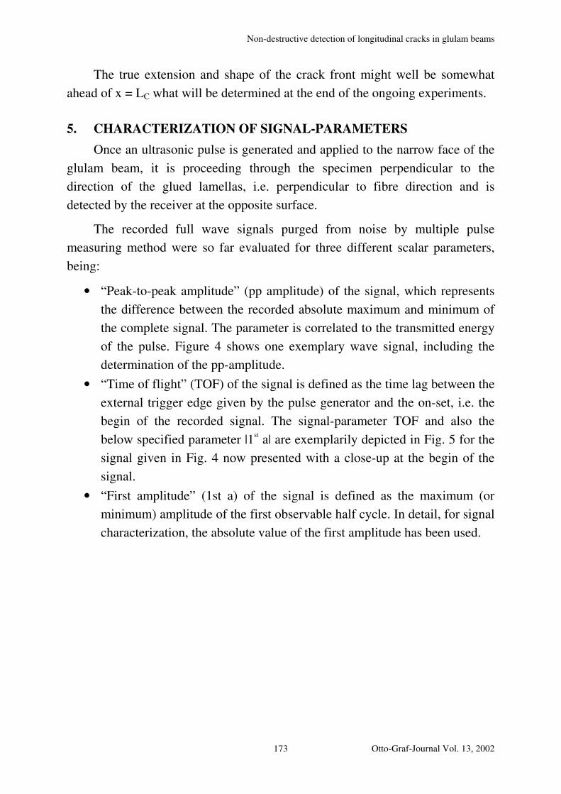
Non-destructive detection of longitudinal cracks in glulam beams
The true extension and shape of the crack front might well be somewhat
ahead of x = LC what will be determined at the end of the ongoing experiments.
5. CHARACTERIZATION OF SIGNAL-PARAMETERS
Once an ultrasonic pulse is generated and applied to the narrow face of the
glulam beam, it is proceeding through the specimen perpendicular to the
direction of the glued lamellas, i.e. perpendicular to fibre direction and is
detected by the receiver at the opposite surface.
The recorded full wave signals purged from noise by multiple pulse
measuring method were so far evaluated for three different scalar parameters,
being:
• “Peak-to-peak amplitude” (pp amplitude) of the signal, which represents
the difference between the recorded absolute maximum and minimum of
the complete signal. The parameter is correlated to the transmitted energy
of the pulse. Figure 4 shows one exemplary wave signal, including the
determination of the pp-amplitude.
• “Time of flight” (TOF) of the signal is defined as the time lag between the
external trigger edge given by the pulse generator and the on-set, i.e. the
begin of the recorded signal. The signal-parameter TOF and also the
below specified parameter |1st a| are exemplarily depicted in Fig. 5 for the
signal given in Fig. 4 now presented with a close-up at the begin of the
signal.
• “First amplitude” (1st a) of the signal is defined as the maximum (or
minimum) amplitude of the first observable half cycle. In detail, for signal
characterization, the absolute value of the first amplitude has been used.
Otto-Graf-Journal Vol. 13, 2002 173

S. AICHER, G. DILL-LANGER, T. RINGGER
a)
0
20
40
0 70 140 210x [cm]
A B Ch [cm]
left face I
LC
beam
depth
h =
440 m
m
b)
0
20
40
0 70 140 210
end of measurable crack(openings > 0.05 mm)x
53.0
cm
67.0
cm
88.4
cm
x [cm]
A B C “left“ face I
“right“ face IIface
Y
face Z
exact shape of crack front unknown
end of visible crackbeam
wid
th
b =
120 m
m
c)
0
20
40
0 70 140 210x [cm]
A B Ch [cm]
right face II
LC
beam
depth
h =
440 m
m
Fig. 3a-c: Schematic illustration of the appearance of the crack at different faces of the specimen. The graphs 3a) and 3c) give measured crack lengths and crack openings (100-times enlarged) at the left and right wide side faces (I and II). Fig 3b shows a projection of the crack area revealing the three crack sections A-C.
174

Non-destructive detection of longitudinal cracks in glulam beams
-3.0
-1.5
0.0
1.5
3.0
0.00 0.20 0.40 0.60 0.80 1.00
time [ms]
signal [V]
pp a
mplit
ude
close upin Fig. 5
Fig. 4: Recorded signal with evaluation / definition of the “peak-to-peak amplitude” (pp amplitude)
-0.4
-0.2
0.0
0.2
0.4
0.00 0.05 0.10 0.15 0.20 0.25
time [ms]
signal [V]
1st a
TOF
Fig. 5 Evaluation / definition of “time of flight” (TOF) and of “first amplitude” (1st a); the graph represents a close-up of the recorded ultrasound pulse given in Fig. 4
Otto-Graf-Journal Vol. 13, 2002 175

S. AICHER, G. DILL-LANGER, T. RINGGER
6. RESULTS OF THE ULTRASOUND MEASUREMENTS
The reproducibility of the signal parameters for repeated independent
measurements at a specific location x (uncoupling and new coupling of the
transducers for each measurement) differed considerably between parameter
TOF on the one side and parameters pp and |1st a| on the other side. In case of
TOF in average an extremely small coefficient of variation (C.O.V.) of 0.3 %
was obtained whereas for the parameters pp and |1st a| the considerably higher
C.O.V.’s were 21% and 24 %, respectively. For the reproducibility test a number
of 10 repeated measurements have been evaluated.
The major results of the performed preliminary investigations are compiled
in Figs. 6 to 8, showing the signal parameters TOF, pp and |1st a| along specimen
axis x. In all graphs the results of the two test runs S1 and S2 with the alternative
transmitter positions at narrow specimen sides T or B are given, and the mean
value of both test runs is shown additionally. Further, the quality of the signal
parameter reproducibility is indicated in all Figures by an error bar with a height
of 2 times of the respective standard deviation (the error bars are not visible in
Fig. 6 due to the very small C.O.V.’s). The visually determined crack length
segments A, B and C are indicated in the graphs, too. Following the results are
discussed in more detail.
Figure 6 specifying “time of flight (TOF)” vs. beam axis x reveals almost
throughout a steep decrease of parameter TOF along crack length segments A, B
and C. It should be emphasized, that the TOF decrease in the investigated case is
apparently not affected by the fact that the crack is not visually detectable at
surface II in crack zone C. For positions x > LC a rather constant TOF value of
253.2 ms is obtained. This gives a mean phase velocity in transverse direction to
fibre of v90 = 0.44 / (253.2*10-6) = 1738 m/s which is in good agreement with
literature data [Buchur 1989] on phase velocities perpendicular to fibre of wood
/ glulam made of European spruce. A comparison of test series S1 and S2
indicates apart from one exception in the crack range A, that the TOF results are
obviously not influenced by transmitter location closer resp. more far from the
crack plane.
176
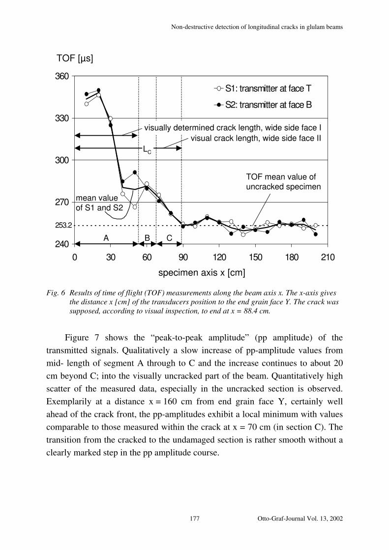
Non-destructive detection of longitudinal cracks in glulam beams
240
270
300
330
360
0 30 60 90 120 150 180 210
S1: transmitter at face T
S2: transmitter at face B
253.2
TOF [µs]
specimen axis x [cm]
visually determined crack length, wide side face I
visual crack length, wide side face II
TOF mean value ofuncracked specimen
A B C
LC
mean valueof S1 and S2
Fig. 6 Results of time of flight (TOF) measurements along the beam axis x. The x-axis gives the distance x [cm] of the transducers position to the end grain face Y. The crack was supposed, according to visual inspection, to end at x = 88.4 cm.
Figure 7 shows the “peak-to-peak amplitude” (pp amplitude) of the
transmitted signals. Qualitatively a slow increase of pp-amplitude values from
mid- length of segment A through to C and the increase continues to about 20
cm beyond C; into the visually uncracked part of the beam. Quantitatively high
scatter of the measured data, especially in the uncracked section is observed.
Exemplarily at a distance x = 160 cm from end grain face Y, certainly well
ahead of the crack front, the pp-amplitudes exhibit a local minimum with values
comparable to those measured within the crack at x = 70 cm (in section C). The
transition from the cracked to the undamaged section is rather smooth without a
clearly marked step in the pp amplitude course.
Otto-Graf-Journal Vol. 13, 2002 177

S. AICHER, G. DILL-LANGER, T. RINGGER
0.0
3.0
6.0
9.0
12.0
15.0
0 30 60 90 120 150 180 210
S1: transmitter at face T
S2: transmitter at face B
pp amplitude [V]
vis. crack lengthwide side face I
vis. crack lengthwide side face II
A B C
specimen axis x [cm]
LC
mean valueof S1 and S2
Fig. 7 Results of peak-to-peak amplitude (pp amplitude) measurements along beam axis x. The x-axis gives the distance x [cm] of the transducers position to the end grain face Y. The crack was supposed according to visual inspection to end at x = 88.4 cm.
Thus, the signal-parameter pp-amplitude does not allow a clear
identification of the crack length. The relatively high uncertainty due to coupling
conditions makes it even more difficult to quantitatively estimate the location of
the crack tip. However, in spite of the scatter, the clearly visible trend of
decreased attenuation for decreasing crack openings is not affected qualitatively.
The presented results for the behaviour of the peak-to-peak amplitude in
case of cracks can be compared to the observations of [KLINGSCH, 1991], where
no damping of pp amplitudes has been measured in the case of saw-cuts.
In Fig. 8 the results of |1st a| along beam axis x are shown for the two
performed test series S1 and S2 together with the boundaries of the different
crack sections.
178
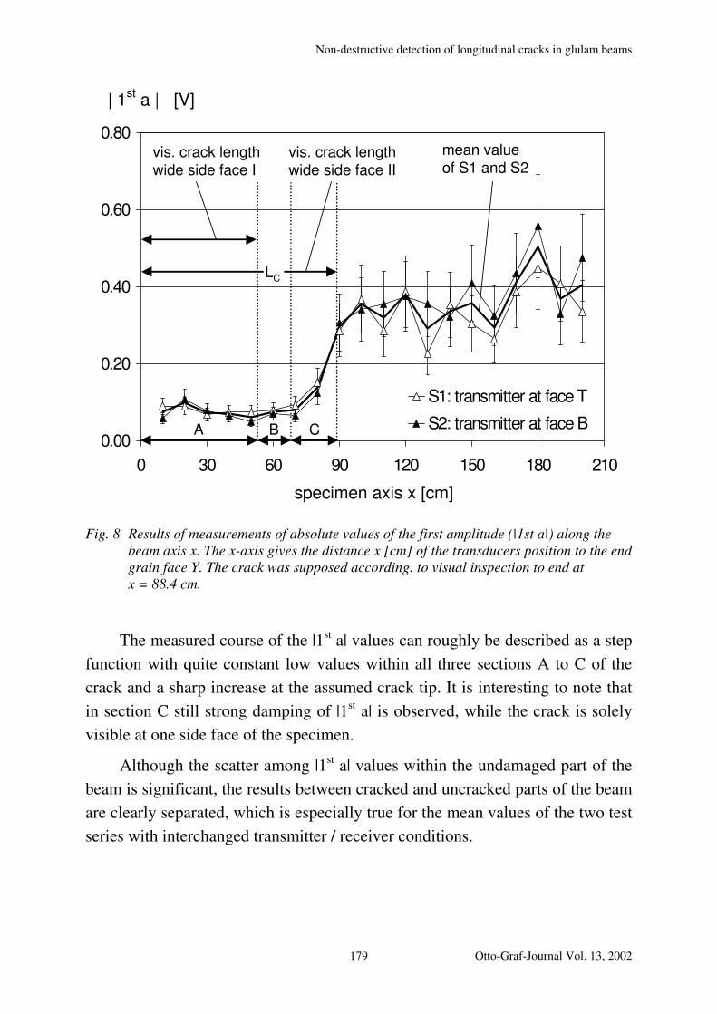
Non-destructive detection of longitudinal cracks in glulam beams
0.00
0.20
0.40
0.60
0.80
0 30 60 90 120 150 180 210
S1: transmitter at face T
S2: transmitter at face B
| 1st a | [V]
vis. crack lengthwide side face I
vis. crack lengthwide side face II
A B C
specimen axis x [cm]
LC
mean valueof S1 and S2
Fig. 8 Results of measurements of absolute values of the first amplitude (|1st a|) along the beam axis x. The x-axis gives the distance x [cm] of the transducers position to the end grain face Y. The crack was supposed according. to visual inspection to end at x = 88.4 cm.
The measured course of the |1st a| values can roughly be described as a step
function with quite constant low values within all three sections A to C of the
crack and a sharp increase at the assumed crack tip. It is interesting to note that
in section C still strong damping of |1st a| is observed, while the crack is solely
visible at one side face of the specimen.
Although the scatter among |1st a| values within the undamaged part of the
beam is significant, the results between cracked and uncracked parts of the beam
are clearly separated, which is especially true for the mean values of the two test
series with interchanged transmitter / receiver conditions.
Otto-Graf-Journal Vol. 13, 2002 179
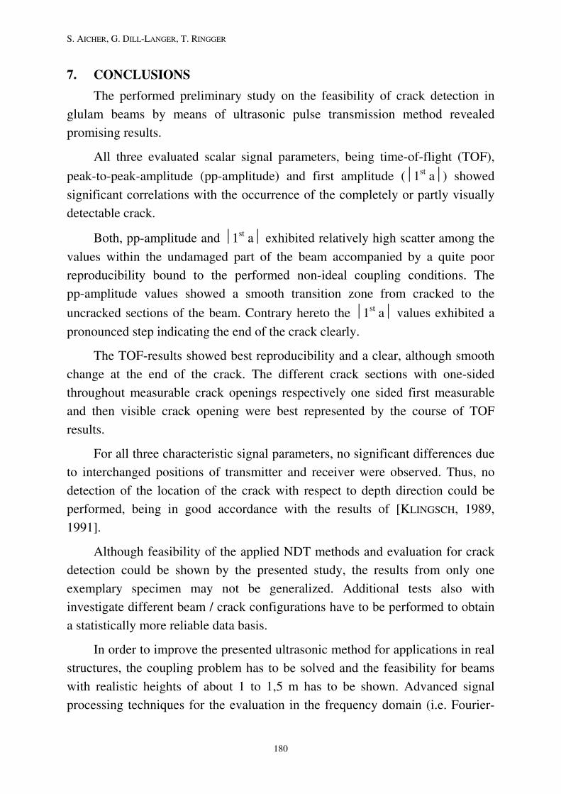
S. AICHER, G. DILL-LANGER, T. RINGGER
7. CONCLUSIONS
The performed preliminary study on the feasibility of crack detection in
glulam beams by means of ultrasonic pulse transmission method revealed
promising results.
All three evaluated scalar signal parameters, being time-of-flight (TOF),
peak-to-peak-amplitude (pp-amplitude) and first amplitude (1st a) showed
significant correlations with the occurrence of the completely or partly visually
detectable crack.
Both, pp-amplitude and 1st a exhibited relatively high scatter among the
values within the undamaged part of the beam accompanied by a quite poor
reproducibility bound to the performed non-ideal coupling conditions. The
pp-amplitude values showed a smooth transition zone from cracked to the
uncracked sections of the beam. Contrary hereto the 1st a values exhibited a
pronounced step indicating the end of the crack clearly.
The TOF-results showed best reproducibility and a clear, although smooth
change at the end of the crack. The different crack sections with one-sided
throughout measurable crack openings respectively one sided first measurable
and then visible crack opening were best represented by the course of TOF
results.
For all three characteristic signal parameters, no significant differences due
to interchanged positions of transmitter and receiver were observed. Thus, no
detection of the location of the crack with respect to depth direction could be
performed, being in good accordance with the results of [KLINGSCH, 1989,
1991].
Although feasibility of the applied NDT methods and evaluation for crack
detection could be shown by the presented study, the results from only one
exemplary specimen may not be generalized. Additional tests also with
investigate different beam / crack configurations have to be performed to obtain
a statistically more reliable data basis.
In order to improve the presented ultrasonic method for applications in real
structures, the coupling problem has to be solved and the feasibility for beams
with realistic heights of about 1 to 1,5 m has to be shown. Advanced signal
processing techniques for the evaluation in the frequency domain (i.e. Fourier-
180
Non-destructive detection of longitudinal cracks in glulam beams
and Wavelet transforms) should be used for noise reduction, enhancement of
resolution and defect sensitivity.
ACKNOWLEDGEMENTS
The authors are very much indebted to Dr. Catherine Lidin (Collano AG,
Switzerland) for the utmost valuable favour translating the abstract and title of
this paper into technically and linguistically correct French.
The financial support of German Science Community (DFG) via grant to
Sonderforschungsbereich 381 "Characterisation of damage evolution in
composite materials using non-destructive test methods" and hereby to sub-
project A8 "Damage and NDT of the natural fibre composite material wood" is
gratefully acknowledged.
REFERENCES
KLINGSCH, W.: Zerstörungsfreie Lokalisierung äußerlich nicht sichtbarer
Holzschädigung. Bauen mit Holz 6, 1989, pp. 421-423
KLINGSCH, W.: Erarbeitung anwendungstechnischer Grundlagen zur
zerstörungsfreien Qualitätsüberwachung von Holzleimbauteilen mittels
Ultraschall. Forschungsbericht, 1991
BUCUR, V.: Acoustics of wood. Boca Raton, New York, London, Tokyo, 1995,
p. 121
KIMURA, M., KUSUNOKI, T., OHTA, M., HATANAKA, K., KOZUKA, H., ITO, H.:
Ultrasonic pulse test on glulam glued connection. Proc. Int. Timber Eng.
Conf., part 2, London, 1991, pp. 2.250 – 2.257
Otto-Graf-Journal Vol. 13, 2002 181

S. AICHER, G. DILL-LANGER, T. RINGGER
182
Determination of local and global modulus of elasticity in wooden boards
DETERMINATION OF LOCAL AND GLOBAL MODULUS OF ELAS-TICITY IN WOODEN BOARDS
BESTIMMUNG DES LOKALEN UND GLOBALEN ELASTIZITÄTS-MODUL IN HOLZBRETTERN
DETERMINATION DU MODULE D’ELASTICITE LOCAL ET GLO-BAL SUR DES PANNEAUX A BASE DE BOIS
Simon Aicher, Lilian Höfflin, Wolfgang Behrens
SUMMARY
The paper reports on an efficient method for determination of the local
modulus of elasticity by means of elongation/strain measurements. Further, the
effect of local weak sections on the global modulus of elasticity determined by
deflection measurement is revealed. The global modulus of elasticity computed
on the basis of the partly extremely varying locally measured moduli of elastic-
ity complies well with the globally measured MOE.
The experimental investigations were performed with edgewise bent beech
boards. First, the elongation /strain measurement method was verified exem-
plary with a board which was inflicted successively with artificial defects
(holes). For each defect state the local and global moduli of elasticity were
measured and the differences are discussed. Second, the variation of local
modulus of elasticity and its high spatial correlation with the location of bending
failure is shown exemplarily by means of four beech boards of a larger test se-
ries.
ZUSAMMENFASSUNG
Es wird über eine effiziente Methode zur Bestimmung des lokalen Elastizi-
tätsmoduls mittels Längsverschiebungs-/Dehnungsmessungen berichtet. Des-
weiteren wird die Auswirkung lokaler Schwachstellen auf den mittels Durchbie-
gungsmessung bestimmten globalen Elastizitätsmodul gezeigt. Der aus den teil-
weise extrem variierenden lokal gemessenen Elastizitätsmoduln berechnete glo-
bale Elastizitätsmodul stimmt sehr gut mit dem gemessenen globalen Elastizi-
tätsmodul überein.
Otto-Graf-Journal Vol. 13, 2002 183

S. AICHER, L. HÖFFLIN, W. BEHRENS
Die experimentellen Untersuchungen wurden mit hochkant biegebean-
spruchten Buchebrettern durchgeführt. Zuerst wurde die Längsverschiebungs-
/Dehnungsmeßmethode exemplarisch an einem Brett verifiziert, welches stu-
fenweise mit künstlichen Defekten (Löchern) versehen wurde. Für jeden De-
fektzustand wurden die lokalen und globalen Elastizitätsmoduln gemessen. In
einem zweiten Schritt wird die Änderung des lokalen Elastizitätsmoduls und
dessen hohe Korrelation mit dem Ort des Biegeversagens exemplarisch an vier
Brettern einer größeren Versuchsreihe aufgezeigt.
RESUME
Cet article présente une méthode efficace permettant de déterminer le mo-
dule d’élasticité local par une mesure couplée déplacement/déformation. D’autre
part, on fait apparaître l’effet des sections localement faibles sur le module
d’élasticité global déterminé par la flèche. Le module d’élasticité global obtenu
par intégration des modules locaux mesurés, extrêmement variables, est en bon
accord avec le module global mesuré.
L’étude expérimentale a porté sur des panneaux fléchis à chant. La mé-
thode couplée déplacement/déformation a été préalablement vérifiée sur un pan-
neau présentant des défauts artificiels (trous). Pour chaque défaut, on détermine
les modules local et global, et les différences sont discutées. Par la suite, la va-
riation du module local et sa forte corrélation spatiale avec la résistance en
flexion est mise en évidence sur 4 panneaux de hêtre extraits d’une campagne
expérimentale plus importante
KEYWORDS: local modulus of elasticity, global modulus of elasticity, stiff-
ness variation, artificial defects, weak sections
1 INTRODUCTION
It is reported on a method for determination of the local modulus of elastic-
ity (MOE) in bending tests with timber beams and respective results. In hetero-
geneous materials such as wood the modulus of elasticity can vary strongly
along the length of the boards. Based on a positive stiffness - bending strength
correlation, the footprints of locally low MOE values determine the strength
class (or grade) of boards in grading machines based on the bending principle.
Local MOE obviously depends strongly on the length of the board segment used
184
Determination of local and global modulus of elasticity in wooden boards
for the MOE determination which in most cases is larger than a local weak area,
mostly created by a knot or by sloping grain.
A local MOE determined over a board segment length of 5 times the cross-
sectional depth as specified in EN 408 still represents an integral (constant)
value over a considerable length and there may be strong local MOE deviations
within that length. The stated averaging effect of concentrated zones of low
MOE areas occurs in all bending type grading machines which bend at consecu-
tive locations, as there are practical limits for the length of the span. This is the
major reason for the moderate coefficient of correlation between bending
strength and MOE. Interesting approaches on how to reconstruct the variation of
the true MOE function from MOE data collected from a consecutively bent
board in order to derive the true local MOEs based on Fourier transforms were
proposed by Bechtel (1985) and Foschi (1987).
Apart from strength grading the knowledge of the actual local MOE and of
the associated local strength variation along the length of boards is very impor-
tant for (stochastic) modelling of boards and glulam subdivided in unit cells of
small length, i.a. Foschi and Barrett (1980), Ehlbeck et al. (1985), Isaksson
(1999) and Serrano (2001). Hereby the length of the unit cell has a considerable
modelling influence on load sharing in adjacent glulam lamellas.
For modelling and calibrating the MOE variation along board length sev-
eral approaches are known (i.a. Foschi and Barrett (1981), Ehlbeck et al. (1985),
Kline at al. (1986) and Taylor (1991)). All models are based on a calibration vs.
global (and partly local) modulus of elasticity necessitating extensive empiric
data and leaving model dependent considerable uncertainties.
The experimental determination of local MOEs which at first view seems
to be a very simple task is demanding in case a bending method is applied and
has limits concerning the smallness of the segment length. Reliable results be-
low span to depth ratios of about 3 are questionable; limits were revealed by
Kaas (1975) employing the so-termed “middle ordinate method”. The method is
based on the assumption that short segments of a bent board approximate arcs of
circles with varying radii.
The work reported here was conducted in the frame of establishing a realis-
tic empirical data basis for the variation of bending MOE and bending strength
values along the length of beech wood boards bent about the major axis. It was
Otto-Graf-Journal Vol. 13, 2002 185

S. AICHER, L. HÖFFLIN, W. BEHRENS
intended to measure the local bending MOE over distances or unit cell lengths in
the range of 1 to 2 times of the depth of the boards.
The paper shows a method for determination of the local modulus of elas-
ticity by means of displacement/strain measurements and reveals the effect of
local weak sections in comparison to the global modulus of elasticity determined
by deflection measurement. The experimental verification of the method which
in principle is independent of specific materials is performed with edgewise
loaded beech boards. First, the displacement/strain measurement method is veri-
fied exemplary with a board which was inflicted successively with artificial de-
fects. For each defect state the local and global modulus of elasticity were meas-
ured and the differences are discussed. Finally, the variation of local modulus of
elasticity and its local correlation with the position of failure is shown exempla-
rily on four beech boards of a larger test series.
2 GLOBAL AND LOCAL METHOD FOR DETERMINATION OF MODULUS OF ELASTICITY IN BENDING
It is important to note that the terms “local MOE” and “global MOE” here
are defined different as in European standard EN 408. In the mentioned standard
the so-termed local MOE is determined in a 4point bending test with loads in the
3rd points via deflection measurement within the constant moment length of 6
times the depth h of the beam. The deflection w1 is actually determined over a
length of `m = 5 h (Fig. 1a). Contrary thereto, so-termed “global MOE” is de-
termined acc. to EN 408 from deflection measurement w2 over full span of 18 h
including effects of shear and of indentations at the support locations (Fig. 1a).
In this paper global MOE is determined similar as local MOE acc. to EN
408 via deflection measurement w1 within an enlarged constant moment area of
9 h. Local MOE is determined by elongation/strain measurement over the length
of a small segment of the beam (see below).
2.1 Global modulus of elasticity
Global MOE based on deflection w1 in the constant moment area is (see
Fig. 1a)
1
2ma
globwI8
FE
``= (1)
with I = moment of inertia vs. major axis.
186
Determination of local and global modulus of elasticity in wooden boards
This measurement delivers an integral value over the length of `m.
2.2 Local modulus of elasticity
For determination of the local modulus of elasticity the bending compli-
ance of the beam was no more determined by deflection measurement but in-
stead by local elongation/strain measurements. The employed measuring princi-
ple is illustrated in Fig. 1b. The method consists of elongation/strain measure-
ments over “small” lengths at the bending tension and compression edge of the
beam. Based on the strains of the segment, εc and εt, the curvature κ of the seg-
ment of length L is given by (h = beam depth)
( )h
tc ε+ε=κ where
L
u )t(c
)t(c
∆=ε . (2a, b)
The bending MOE of the segment is then obtained from the curvature-moment
relationship
I
MEseg
κ= with M = F `a (3)
The introduced elongation/strain measurement method is limited to small
deflections; the arc length of the bending line of the beam segment has to be ap-
proximately equal to its chord length. This is the case for small ratios of L/h.
Here length L was chosen with respect to modelling aspects (smallest employed
“cell” size), not discussed in this paper, in conjunction with existing equipment
as L = 200 mm. This is roughly 1.5 times the depth of the investigated beams.
The determination of the elongations can be performed very accurately, say re-
producible, by means of so-called on-set strain extensometers. Despite the mis-
leading term “strain extensometer” the measurement actually represents an
elongation measurement of an exactly determined base length L. In order to es-
tablish the base length, small fixing plates (∅ 8 mm) with a conical hole for the
pin pointed extensometer legs are glued (wax) to the measured object, here to
the narrow faces of the beam.
Otto-Graf-Journal Vol. 13, 2002 187
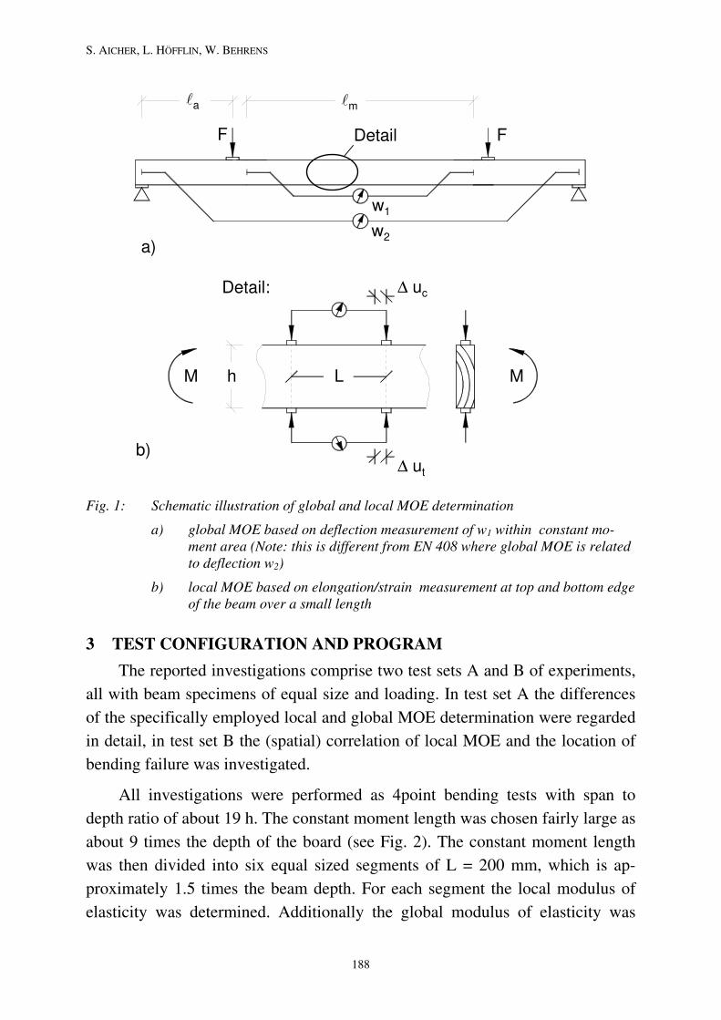
S. AICHER, L. HÖFFLIN, W. BEHRENS
w1
w2
M M L
∆ uc
∆ ut
Detail
Detail:
`a `m
F F
a)
b)
h
Fig. 1: Schematic illustration of global and local MOE determination
a) global MOE based on deflection measurement of w1 within constant mo-ment area (Note: this is different from EN 408 where global MOE is related to deflection w2)
b) local MOE based on elongation/strain measurement at top and bottom edge of the beam over a small length
3 TEST CONFIGURATION AND PROGRAM
The reported investigations comprise two test sets A and B of experiments,
all with beam specimens of equal size and loading. In test set A the differences
of the specifically employed local and global MOE determination were regarded
in detail, in test set B the (spatial) correlation of local MOE and the location of
bending failure was investigated.
All investigations were performed as 4point bending tests with span to
depth ratio of about 19 h. The constant moment length was chosen fairly large as
about 9 times the depth of the board (see Fig. 2). The constant moment length
was then divided into six equal sized segments of L = 200 mm, which is ap-
proximately 1.5 times the beam depth. For each segment the local modulus of
elasticity was determined. Additionally the global modulus of elasticity was
188

Determination of local and global modulus of elasticity in wooden boards
global deflection measurement w1 over ≈ 9 h
Detail, seeFigs. 2b - d
` = 2460
`a = 555 `m = 6 x L = 1200 `a = 555
b = 40
h =
129
L = 200
75 75
1350
a)
seg-ment 1 2 543 6
seg-ment 1 2
543 6
seg-ment 1 2 54
36
Detail (test A1 and test set B)
3 holes ∅
25 mm
3 holes ∅
25 mm
Extensometer
Detail (test A2)
Detail (test A3)4 x 50
4 x 50
h/4h/4
h/2
h/4h/4
h/2
b)
d)
c)
Fig. 2a-d: investigated specimen and loading configurations in test sets A and B
a) general test set-up
b) test A1(with board No. 1) and test set B; only natural defects (if at all) in segments 1 – 6
c) test A2; 3 artificial holes in segment 5 of board No. 1
d) test A3; 3 additional artificial holes in segment 3 of board No. 1
Otto-Graf-Journal Vol. 13, 2002 189
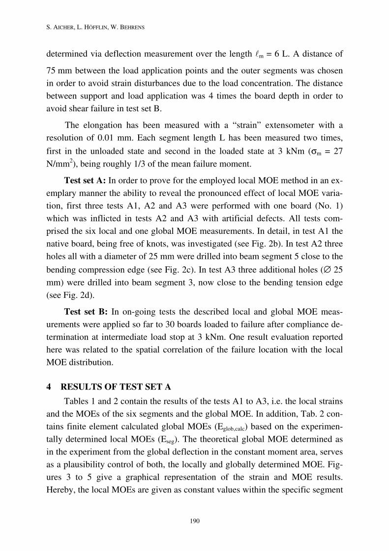
S. AICHER, L. HÖFFLIN, W. BEHRENS
determined via deflection measurement over the length `m = 6 L. A distance of
75 mm between the load application points and the outer segments was chosen
in order to avoid strain disturbances due to the load concentration. The distance
between support and load application was 4 times the board depth in order to
avoid shear failure in test set B.
The elongation has been measured with a “strain” extensometer with a
resolution of 0.01 mm. Each segment length L has been measured two times,
first in the unloaded state and second in the loaded state at 3 kNm (σm = 27
N/mm2), being roughly 1/3 of the mean failure moment.
Test set A: In order to prove for the employed local MOE method in an ex-
emplary manner the ability to reveal the pronounced effect of local MOE varia-
tion, first three tests A1, A2 and A3 were performed with one board (No. 1)
which was inflicted in tests A2 and A3 with artificial defects. All tests com-
prised the six local and one global MOE measurements. In detail, in test A1 the
native board, being free of knots, was investigated (see Fig. 2b). In test A2 three
holes all with a diameter of 25 mm were drilled into beam segment 5 close to the
bending compression edge (see Fig. 2c). In test A3 three additional holes (∅ 25
mm) were drilled into beam segment 3, now close to the bending tension edge
(see Fig. 2d).
Test set B: In on-going tests the described local and global MOE meas-
urements were applied so far to 30 boards loaded to failure after compliance de-
termination at intermediate load stop at 3 kNm. One result evaluation reported
here was related to the spatial correlation of the failure location with the local
MOE distribution.
4 RESULTS OF TEST SET A
Tables 1 and 2 contain the results of the tests A1 to A3, i.e. the local strains
and the MOEs of the six segments and the global MOE. In addition, Tab. 2 con-
tains finite element calculated global MOEs (Eglob,calc) based on the experimen-
tally determined local MOEs (Eseg). The theoretical global MOE determined as
in the experiment from the global deflection in the constant moment area, serves
as a plausibility control of both, the locally and globally determined MOE. Fig-
ures 3 to 5 give a graphical representation of the strain and MOE results.
Hereby, the local MOEs are given as constant values within the specific segment
190
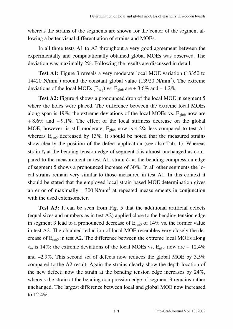
Determination of local and global modulus of elasticity in wooden boards
whereas the strains of the segments are shown for the center of the segment al-
lowing a better visual differentiation of strains and MOEs.
In all three tests A1 to A3 throughout a very good agreement between the
experimentally and computationally obtained global MOEs was observed. The
deviation was maximally 2%. Following the results are discussed in detail:
Test A1: Figure 3 reveals a very moderate local MOE variation (13350 to
14420 N/mm2) around the constant global value (13920 N/mm2). The extreme
deviations of the local MOEs (Eseg) vs. Eglob are + 3.6% and – 4.2%.
Test A2: Figure 4 shows a pronounced drop of the local MOE in segment 5
where the holes were placed. The difference between the extreme local MOEs
along span is 19%; the extreme deviations of the local MOEs vs. Eglob now are
+ 8.6% and – 9.1%. The effect of the local stiffness decrease on the global
MOE, however, is still moderate; Eglob now is 4.2% less compared to test A1
whereas Eseg5 decreased by 13%. It should be noted that the measured strains
show clearly the position of the defect application (see also Tab. 1). Whereas
strain εt at the bending tension edge of segment 5 is almost unchanged as com-
pared to the measurement in test A1, strain εc at the bending compression edge
of segment 5 shows a pronounced increase of 30%. In all other segments the lo-
cal strains remain very similar to those measured in test A1. In this context it
should be stated that the employed local strain based MOE determination gives
an error of maximally ± 300 N/mm2 at repeated measurements in conjunction
with the used extensometer.
Test A3: It can be seen from Fig. 5 that the additional artificial defects
(equal sizes and numbers as in test A2) applied close to the bending tension edge
in segment 3 lead to a pronounced decrease of Eseg3 of 14% vs. the former value
in test A2. The obtained reduction of local MOE resembles very closely the de-
crease of Eseg5 in test A2. The difference between the extreme local MOEs along
`m is 14%; the extreme deviations of the local MOEs vs. Eglob now are + 12.4%
and –2.9%. This second set of defects now reduces the global MOE by 3.5%
compared to the A2 result. Again the strains clearly show the depth location of
the new defect; now the strain at the bending tension edge increases by 24%,
whereas the strain at the bending compression edge of segment 3 remains rather
unchanged. The largest difference between local and global MOE now increased
to 12.4%.
Otto-Graf-Journal Vol. 13, 2002 191

S. AICHER, L. HÖFFLIN, W. BEHRENS
Table 1: Compilation of local compression and tension strains of test set A
1 2 3 4 5 6
εc 10-5 -62.4 -60.4 -58.7 -64.9 -61.3 -60.2
εt 10-5 71.2 66.8 66.7 70.2 67.5 64.9
εc 10-5 -63.3 -59.5 -57.8 -66.7 -79.4 -62.9
εt 10-5 70.3 66.8 66.6 70.2 68.4 64.9
εc 10-5 -61.5 -57.7 -61.4 -66.7 -74.0 -61.1
εt 10-5 70.3 66.8 82.8 72.0 68.4 64.9
A2
A3
compression
and tension
strain per 1kNm
local strains in segments 1 to 6test
A1
Table 2: Compilation of results for local and global MOEs of test set A
global
measured
MOE
calculated MOE based
on the measured local
MOEs
Eseg1 Eseg2 Eseg3 Eseg4 Eseg5 Eseg6 Eglob Eglob, calc
- N/mm2
N/mm2
N/mm2
N/mm2
N/mm2
N/mm2
N/mm2
N/mm2
A1 13495 14172 14381 13347 13989 14415 13919 13932
A2 13494 14272 14493 13171 12197 14110 13340 13576
A3 13686 14479 12502 13000 12660 14311 12879 13141
test measured local MOEs in segments 1 to 6
12000
12500
13000
13500
14000
14500
15000
segment
modulu
s o
f ela
sticity [
N/m
m2]
55
60
65
70
75
80
85str
ain
[10
-5/k
Nm
]
1 2 3 4 5 6
Eseg Eglob |εc| εt
Fig. 3: Local strains, local and global MOEs of test A1 with board No. 1; no artificial defects
192
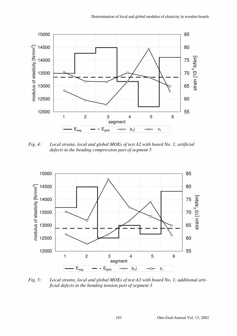
Determination of local and global modulus of elasticity in wooden boards
12000
12500
13000
13500
14000
14500
15000
segment
mo
du
lus o
f e
lasticity [
N/m
m2]
55
60
65
70
75
80
85
str
ain
[10
-5/k
Nm
]
1 2 3 4 5 6
Eseg Eglob |εc| εt
Fig. 4: Local strains, local and global MOEs of test A2 with board No. 1; artificial defects in the bending compression part of segment 5
12000
12500
13000
13500
14000
14500
15000
segment
mo
du
lus o
f e
lasticity [
N/m
m2]
55
60
65
70
75
80
85
str
ain
[10
-5/k
Nm
]
1 2 3 4 5 6
Eseg Eglob |εc| εt
Fig. 5: Local strains, local and global MOEs of test A3 with board No. 1; additional arti-ficial defects in the bending tension part of segment 3
Otto-Graf-Journal Vol. 13, 2002 193
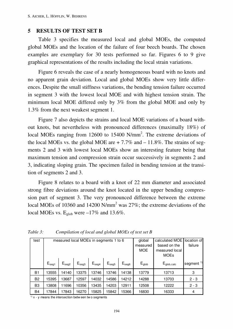
S. AICHER, L. HÖFFLIN, W. BEHRENS
5 RESULTS OF TEST SET B
Table 3 specifies the measured local and global MOEs, the computed
global MOEs and the location of the failure of four beech boards. The chosen
examples are exemplary for 30 tests performed so far. Figures 6 to 9 give
graphical representations of the results including the local strain variations.
Figure 6 reveals the case of a nearly homogeneous board with no knots and
no apparent grain deviation. Local and global MOEs show very little differ-
ences. Despite the small stiffness variations, the bending tension failure occurred
in segment 3 with the lowest local MOE and with highest tension strain. The
minimum local MOE differed only by 3% from the global MOE and only by
1.3% from the next weakest segment 1.
Figure 7 also depicts the strains and local MOE variations of a board with-
out knots, but nevertheless with pronounced differences (maximally 18%) of
local MOEs ranging from 12600 to 15400 N/mm2. The extreme deviations of
the local MOEs vs. the global MOE are + 7.7% and – 11.8%. The strains of seg-
ments 2 and 3 with lowest local MOEs show an interesting feature being that
maximum tension and compression strain occur successively in segments 2 and
3, indicating sloping grain. The specimen failed in bending tension at the transi-
tion of segments 2 and 3.
Figure 8 relates to a board with a knot of 22 mm diameter and associated
strong fibre deviations around the knot located in the upper bending compres-
sion part of segment 3. The very pronounced difference between the extreme
local MOEs of 10360 and 14200 N/mm2 was 27%; the extreme deviations of the
local MOEs vs. Eglob were –17% and 13.6%.
Table 3: Compilation of local and global MOEs of test set B
global
measured
MOE
calculated MOE
based on the
measured local
MOEs
location of
failure
Eseg1 Eseg2 Eseg3 Eseg4 Eseg5 Eseg6 Eglob Eglob,calc segment 1)
B1 13555 14140 13375 13746 13746 14138 13779 13713 3
B2 15395 13687 12597 14032 14586 14212 14288 13703 2 - 3
B3 13808 11696 10356 13435 14203 12911 12508 12222 2 - 3
B4 17844 17843 16270 15825 15842 15366 16830 16333 41) x - y means the intersection betw een tw o segments
test measured local MOEs in segments 1 to 6
194

Determination of local and global modulus of elasticity in wooden boards
12000
13000
14000
15000
16000
17000
segment
modulu
s o
f ela
sticity [
N/m
m2]
40
45
50
55
60
65
str
ain
[10
-5/k
Nm
]
1 2 3 4 5 6
Eseg Eglob |εc| εt
area of failure initiation
Fig. 6: Local strains, local and global MOEs of test B1 (board No. 416)
11000
12000
13000
14000
15000
16000
segment
mo
du
lus o
f e
lasticity [N
/mm
2]
45
50
55
60
65
70
str
ain
[10
-5/k
Nm
]
1 2 3 4 5 6
area of failure initiation
Eseg Eglob |εc| εt
Fig. 7: Local strains, local and global MOEs of test B2 (board No. 258)
The specimen failed as sole specimen in the tests so far in bending compression
at the transition of segments 2 and 3 with highest compression strains and lowest
local MOE, respectively.
Otto-Graf-Journal Vol. 13, 2002 195

S. AICHER, L. HÖFFLIN, W. BEHRENS
10000
11000
12000
13000
14000
15000
segment
mo
du
lus o
f e
lasticity [
N/m
m2]
50
60
70
80
90
100
str
ain
[10
-5/k
Nm
]
1 2 3 4 5 6
Eseg Eglob |εc| εt
area of failure initiation
Fig. 8: Local strains, local and global MOEs of test B3 (board No. 281)
14000
15000
16000
17000
18000
19000
segment
mo
du
lus o
f e
lasticity [
N/m
m2]
40
45
50
55
60
65
str
ain
[10
-5/k
Nm
]
1 2 3 4 5 6
Eseg Eglob |εc| εt
area of failure initiation
Fig. 9: Local strains, local and global MOEs of test B4 (board No. 213)
Figure 9 shows strains and MOEs of a board without knots and absolutely
very “high” MOEs with a global MOE of 16830 N/mm2. Bending compression
and tension strains are very similar. The specimen failed in bending tension in
segment 4 with the second lowest MOE. However, local MOEs in segments 4, 5
and 6 are very similar and deviate maximally by 2% from their respective mean.
196

Determination of local and global modulus of elasticity in wooden boards
Again, as in test set A, a very good agreement between the experimentally
and computationally obtained global MOEs was observed. The deviation was in
average 2.4% and maximally 3.7%.
6 DISCUSSION
The results show that the employed method is able to deliver local MOEs
and therefore to reveal the MOE variation within a board. However, the meas-
ured local MOEs still do not represent the true MOEs of the zones with or with-
out defects within the board. The measured MOE depends to a great extent on
the gauge (segment) length, L, the length of the weak area and also on the rela-
tive differences of the stiffness within the gauge length. The smaller the chosen
segment length, the smaller the difference between the measured and the “true”
MOE. The employed gauge length of about 1.5 times the board depth seems to
be in the size range of typical defect zones of the regarded wood species as the
results show a good correlation between the minimum localized MOE value and
location of bending failure. However, some improvement should still be ob-
tained by a further reduction of gauge length L.
7 CONCLUSIONS
The presented results show that determination of the local modulus of elas-
ticity in (edgewise) bending can be well performed by elongation/strain meas-
urement at the bending tension and compression edges.
The measured local MOEs and the experimental global MOE obtained from de-
flection measurement, are consistent. This results from the fact that the global
MOE can be predicted by beam theory or FE analysis with an average error of
about 2% on the basis of the local MOE of the segments, here chosen with a
length of 200 mm.
It was revealed that the locations of failure comply well with the locations of
minimum MOE along beam length (the study so far comprised 30 beech
boards). The presented method seems to enable the prediction of the type of
bending failure either at the tension or compression edge.
The data of the on-going study serve as a calibration basis for modelling of the
variation of modulus of elasticity and bending strength along beech wood boards
as input data for glued compound elements with edgewise bent lamellas.
Otto-Graf-Journal Vol. 13, 2002 197
S. AICHER, L. HÖFFLIN, W. BEHRENS
ACKNOWLEDGEMENTS
The authors want to express sincere thanks to Patrick Castera, head of La-
boratoire du Bois de Bordeaux (LRBB), for his repeated favour in performing
the translation of the French abstract.
REFERENCES
BECHTEL, F.K. (1985): Beam stiffness as a function of point wise E, with applica-
tion to machine stress rating. Proceedings International Symposium on
Forest Products Research, CSIR, Pretoria, South Africa
CORDER, S.E. (1965): Localized deflection related to bending strength of lumber.
Second Symposium on the Non-destructive Testing of Wood, Washington
State University, Pullman, WA, pp. 461 – 473
EHLBECK, J., COLLING, F., GÖRLACHER, R. (1985): Einfluß keilgezinkter Lamellen
auf die Biegefestigkeit von Brettschichtholzträgern. Entwicklung eines Re-
chenmodells. Holz Roh- Werkstoff, 43, pp. 333 – 337
FOSCHI, R.O., BARRETT, D. (1980): Glued-laminated beam strength: A model. J.
of the Structural Div., Vol. 106, No. ST8, pp. 1735 – 1754
FOSCHI, R.O. (1987): A procedure for the determination of localized modulus of
elasticity. Holz Roh- Werkstoff, 45, pp. 257 – 260
ISAKSSON, T. (1999): Modeling the variability of bending strength in structural
timber; length and load configuration effects. Report MBK-1015, Div. of
Structural Eng., Institute of Technology, Lund, Sweden
KASS, A.J. (1975): Middle ordinate method measures stiffness variation within
pieces of lumber. Forest Products J., 25 (3), pp. 33 – 41
KLINE, D.E., WOESTE, F.E., BENDTSEN, B.A. (1986): Stochastic model for modulus
of elasticity of lumber. Wood and Fibre Science, 18 (2), pp. 228 - 238
SERRANO, E. (2001): Mechanical performance and modeling of glulam. Manu-
script for „Timber Engineering“, Edts. S. Thelandersson and H.J. Larsen,
Wiley & Sons, in press
TAYLOR, S.E., BENDER, D.A. (1991): Stochastic model for localized tensile
strength and modulus of elasticity in lumber. Wood and Fibre Science,
23(4), pp. 501 - 519
198
Transient temperature evolution in glulam with hidden and non-hidden glued-in steel rods
TRANSIENT TEMPERATURE EVOLUTION IN GLULAM WITH HIDDEN AND NON-HIDDEN GLUED-IN STEEL RODS
TRANSIENTE TEMPERATURENTWICKLUNG IN BRETTSCHICHT-HOLZ MIT VERDECKT UND NICHT VERDECKT EINGEKLEBTEN STAHLSTANGEN
EVOLUTION TRANSITOIRE DE LA TEMPERATURE DANS DU LAMELLE COLLE COMPORTANT DES GOUJONS COLLES EN ACIER, APPARENTS OU NON
Simon Aicher, Dirk Kalka, Ralf Scherer
SUMMARY
A recently terminated European research project on glued-in steel rods in
timber structures (GIROD) – with participation of Timber Department of Otto-
Graf-Institute – revealed a strong strength reducing influence of elevated tem-
peratures, not expected to that extent. This affects especially the duration of load
behavior of the connections. The maximum temperature level acting in service
on the glued-in rod connections thus sets performance requirements on the shear
modulus-temperature relationship and on the glass transition temperature of ap-
propriate adhesives.
Today’s prevailing intuitive conviction of practitioners is, that rods bonded
hidden in the interior of glulam cross-sections experience, due to the low ther-
mal conductivity and specific heat of wood, considerable lower temperatures
compared to ambient climate. The paper gives some experimental and computa-
tional results proving, depending on cross-sectional width, only a moderate re-
duction of peak temperatures combined with a pronounced phase shift vs. ambi-
ent temperature varying roughly sinusoidally during a day.
ZUSAMMENFASSUNG
Ein kürzlich abgeschlossenes Europäisches Forschungsvorhaben betreffend
in Holz eingeklebter Stahlstangen (GIROD) – mit Beteiligung des Fachbereichs
Holz des Otto-Graf-Instituts – zeigte einen in dieser Ausprägung nicht erwarte-
ten großen festigkeitsmindernden Einfluss erhöhter Temperaturen. Dies beein-
flusst insbesondere auch das Zeitstandverhalten der Verbindungen. Das maxi-
Otto-Graf-Journal Vol. 13, 2002 199

S. AICHER, D. KALKA, R. SCHERER
male Temperaturniveau, das im Gebrauchszustand auf Verbindungen mit einge-
klebten Stangen einwirkt, definiert somit Leistungsanforderungen an die
Schubmodul-Temperaturbeziehung und an die Glasübergangstemperatur geeig-
neter Klebstoffe.
Die heute in der Praxis vorherrschende Meinung ist, dass verdeckt in das
Innere eines Brettschichtholzquerschnitts eingeklebte Stangen infolge der nied-
rigen Wärmeleitfähigkeit und Wärmekapazität von Holz beträchtlich niedrigeren
Temperaturen im Vergleich zum einwirkenden Umgebungsklima ausgesetzt
sind. Der Aufsatz berichtet über einige experimentelle und rechnerische Ergeb-
nisse, die belegen, dass abhängig von der Querschnittsdicke lediglich eine
schwache Reduzierung der Spitzentemperaturen verbunden mit einer ausgepräg-
ten Phasenverschiebung gegenüber den Außentemperaturen, die näherungsweise
sinusförmig über den Tag variieren, vorliegt.
RESUME
Un projet de recherche Européen portant sur les goujons collés en acier
dans les structures en bois (GIROD) récemment achevé – auquel participait le
département bois de l’Otto-Graf Institute – a mis en évidence un effet négatif
marqué de températures élevées sur la résistance, qui affecte principalement la
durée de vie des joints. La température maximale agissant sur les joints en ser-
vice impose donc des exigences de performance sur la relation température –
module de cisaillement et la température de transition vitreuse des adhésifs ap-
propriés.
La conviction intuitive des praticiens aujourd’hui est de penser que les gou-
jons collés cachés à l’intérieur des sections de lamellé collé sont soumis, du fait
de la faible conductivité thermique et chaleur spécifique du bois, à des tempéra-
tures considérablement plus faibles que celles du climat ambiant. Cet article pré-
sente des résultats expérimentaux et numériques montrant, selon la largeur de la
section, une faible réduction seulement des températures de pic combinée à une
transition de phase prononcée, par rapport à la température ambiante qui varie
grossièrement de manière sinusoïdale au cours d’une journée.
KEYWORDS: glued-in rods, glulam, elevated temperatures, transient tempera-
ture evolution
200
Transient temperature evolution in glulam with hidden and non-hidden glued-in steel rods
1. INTRODUCTION
Today’s prevailing conviction of practitioners is, that steel rods bonded
hidden in the interior of glulam cross-sections experience, due to the low ther-
mal conductivity and specific heat of wood, considerable lower temperatures
compared to ambient climate. A European research project on glued-in rods in
timber structures (GIROD) revealed an unexpected strong strength reducing in-
fluence of elevated temperatures in duration of load tests with connections
bonded by epoxy and polyurethane adhesives [BENGTSSON, JOHANSSON, 2002;
AICHER, 2002].
In the performed tests the temperature increase was applied after mechani-
cal loading thus suppressing positive post-curing effects. The experiments re-
vealed clearly the crucial importance of a sufficiently high glass transition tem-
perature. Performance requirements on temperature stability – especially shear
modulus-temperature relationships and/or glass transition temperature – have to
be set in view of realistic temperature loading scenarios. Eventually the tempera-
ture loading should also be considered in probabilistic manner, in case a specific
adhesive shows high post-curing potential.
The reported experimental investigations were performed in first instance
to substantiate the GIROD results. In addition thereto a major point of interest
was the transient temperature evolution in the timber-bond line interface.
2. TEST PROGRAM
In order to verify the different temperature-strength behavior of glued-in
steel rods either protruding or fully hidden in the wood, two types of specimens
shown in Fig. 1 were investigated. The performed experiments concerned the
strength verification at variable temperature and static long term loads and fur-
thermore the temperature evolution in the bond lines. This paper reports on the
temperature evolution.
The temperatures in the bond line were measured with thermo-elements
consisting of copper/constantan (Cu/Cu-Ni) wires. In order to measure the tem-
peratures in the bond line with little interfering influences of leakages to ambient
climate, the application of the thermo-element wires to the bond line was per-
formed as following: first an oversized specimen was sawn up lengthwise with a
saw blade thickness of 2 mm. Then the two parts were clamped together and a
hole with a diameter of 13 mm for the glued-in rod was drilled. The thermo-
Otto-Graf-Journal Vol. 13, 2002 201
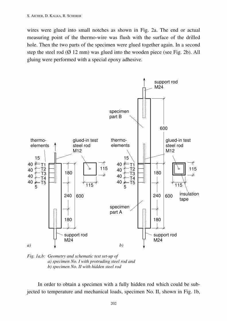
S. AICHER, D. KALKA, R. SCHERER
wires were glued into small notches as shown in Fig. 2a. The end or actual
measuring point of the thermo-wire was flush with the surface of the drilled
hole. Then the two parts of the specimen were glued together again. In a second
step the steel rod (Ø 12 mm) was glued into the wooden piece (see Fig. 2b). All
gluing were performed with a special epoxy adhesive.
a) b)
specimen part A
specimen part B
thermo-elements
thermo-elements
support rod M24
glued-in test steel rod M12
115
115 T1
T5
T2 T3 T4
40
40
40
40 5
15
240
180
180
600 insulation tape
support rodM24
600
support rodM24
glued-in test steel rod M12
115
240
180
180
600
115 T1
T5
T2 T3T4
40
40
40
405
15
Fig. 1a,b: Geometry and schematic test set-up of a) specimen No. I with protruding steel rod and b) specimen No. II with hidden steel rod
In order to obtain a specimen with a fully hidden rod which could be sub-
jected to temperature and mechanical loads, specimen No. II, shown in Fig. 1b,
202
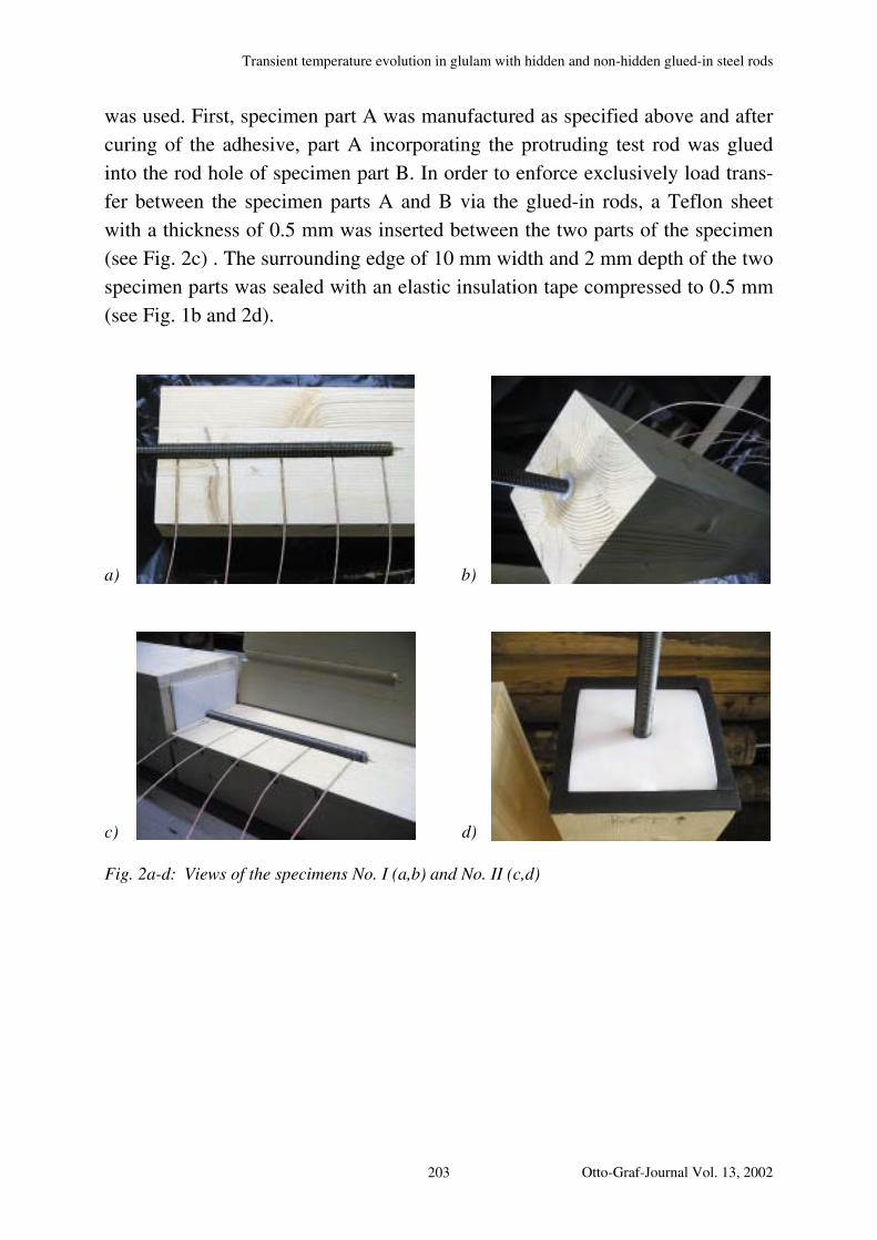
Transient temperature evolution in glulam with hidden and non-hidden glued-in steel rods
was used. First, specimen part A was manufactured as specified above and after
curing of the adhesive, part A incorporating the protruding test rod was glued
into the rod hole of specimen part B. In order to enforce exclusively load trans-
fer between the specimen parts A and B via the glued-in rods, a Teflon sheet
with a thickness of 0.5 mm was inserted between the two parts of the specimen
(see Fig. 2c) . The surrounding edge of 10 mm width and 2 mm depth of the two
specimen parts was sealed with an elastic insulation tape compressed to 0.5 mm
(see Fig. 1b and 2d).
a) b)
c) d)
Fig. 2a-d: Views of the specimens No. I (a,b) and No. II (c,d)
Otto-Graf-Journal Vol. 13, 2002 203
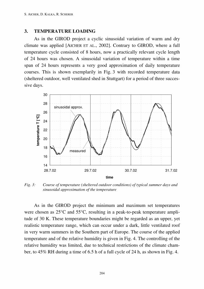
S. AICHER, D. KALKA, R. SCHERER
3. TEMPERATURE LOADING
As in the GIROD project a cyclic sinusoidal variation of warm and dry
climate was applied [AICHER ET AL., 2002]. Contrary to GIROD, where a full
temperature cycle consisted of 8 hours, now a practically relevant cycle length
of 24 hours was chosen. A sinusoidal variation of temperature within a time
span of 24 hours represents a very good approximation of daily temperature
courses. This is shown exemplarily in Fig. 3 with recorded temperature data
(sheltered outdoor, well ventilated shed in Stuttgart) for a period of three succes-
sive days.
14
16
18
20
22
24
26
28
30
28.7.02 29.7.02 30.7.02 31.7.02
time
tem
pera
ture
T [
°C]
sinusoidal approx.
measured
Fig. 3: Course of temperature (sheltered outdoor conditions) of typical summer days and
sinusoidal approximation of the temperature
As in the GIROD project the minimum and maximum set temperatures
were chosen as 25°C and 55°C, resulting in a peak-to-peak temperature ampli-
tude of 30 K. These temperature boundaries might be regarded as an upper, yet
realistic temperature range, which can occur under a dark, little ventilated roof
in very warm summers in the Southern part of Europe. The course of the applied
temperature and of the relative humidity is given in Fig. 4. The controlling of the
relative humidity was limited, due to technical restrictions of the climate cham-
ber, to 45% RH during a time of 6.5 h of a full cycle of 24 h, as shown in Fig. 4.
204

Transient temperature evolution in glulam with hidden and non-hidden glued-in steel rods
The actual temperatures obtained in the climate chamber showed a mini-
mum and maximum of 24.9°C and 54.7°C, respectively, with a peak-to-peak
temperature amplitude of 29.8 K. The relative humidity roughly ranged from 5
to 50 %, exceptionally temporary up to 67 % for about 0.5 hours.
0
10
20
30
40
50
60
70
0 12 24 36 48 60 72 84 96 108 120
time t [h]
tem
pera
ture
T [
°C]
/
rela
tive h
um
idit
y R
H [
%] T
RH
Fig. 4: Course of the applied ambient temperature and relative humidity variation in the climate chamber
4. NUMERICAL INVESTIGATIONS
In an early paper the evolution of temperature in a specimen with a glued-
in rod protruding into ambient air was investigated numerically and experimen-
tally [AICHER ET AL, 1998], taking into account the timber, the adhesive layer
and the steel. An additional fourth layer, representing a steel/adhesive interface,
was introduced in order to account for the problem that the used FE-code does
not enable the specification of contact conductance of inner surfaces. By means
of the interface layer a good agreement of measured and calculated transient
temperatures was obtained.
Otto-Graf-Journal Vol. 13, 2002 205
S. AICHER, D. KALKA, R. SCHERER
In this paper the preliminary numerical study is exclusively related to
specimen No. II with the hidden rod. In a first crude approximation the inner
steel rod was omitted, so only the heat transfer through a quadratic block of tim-
ber was regarded in a 2 dimensional analysis. The cross-sectional dimensions of
the timber, a = 115 mm, were reduced by the hole diameter of 13 mm (rod
diameter + 1 mm) to 102 mm.
In the calculations a constant thermal diffusivity perpendicular to grain of
h
²mm700
C
kD
P ρ
was employed. Hereby k , CP and ρ were assumed as
Km
W13.0k
thermal conductivity perpendicular to fiber
acc. to DIN 4108, part 4
Kkg
kJ6.1CP specific heat [BATZER, 1985]
³m
kg420ρ
mass density of glulam at dry status of about
u = 7 %
The convection heat transfer coefficient h was chosen as a fitting parameter
in the range of 10 to 20 W/(m²·K). Literature data for forced convection of gas
media vary roughly between 10 and 100 W/(m²·K); a value of 25 W/(m²·K) is
assumed for convection at exterior walls in DIN 4108, part 4.
5. TEMPERATURE EVOLUTION IN CYCLIC CLIMATE
Figs. 5a,b show the temperature evolution of both specimen types I and II
at different thermo-element positions. The evolution of the ambient temperature
in the climate chamber is given, too. For a better visualization of phase shift and
differences in amplitudes Figs. 6a and b show the temperature evolution at a cy-
cle length of 24 hours; additionally finite element computed temperature evolu-
tions based on the revealed approach are specified in case of specimen type II
with a hidden rod.
206
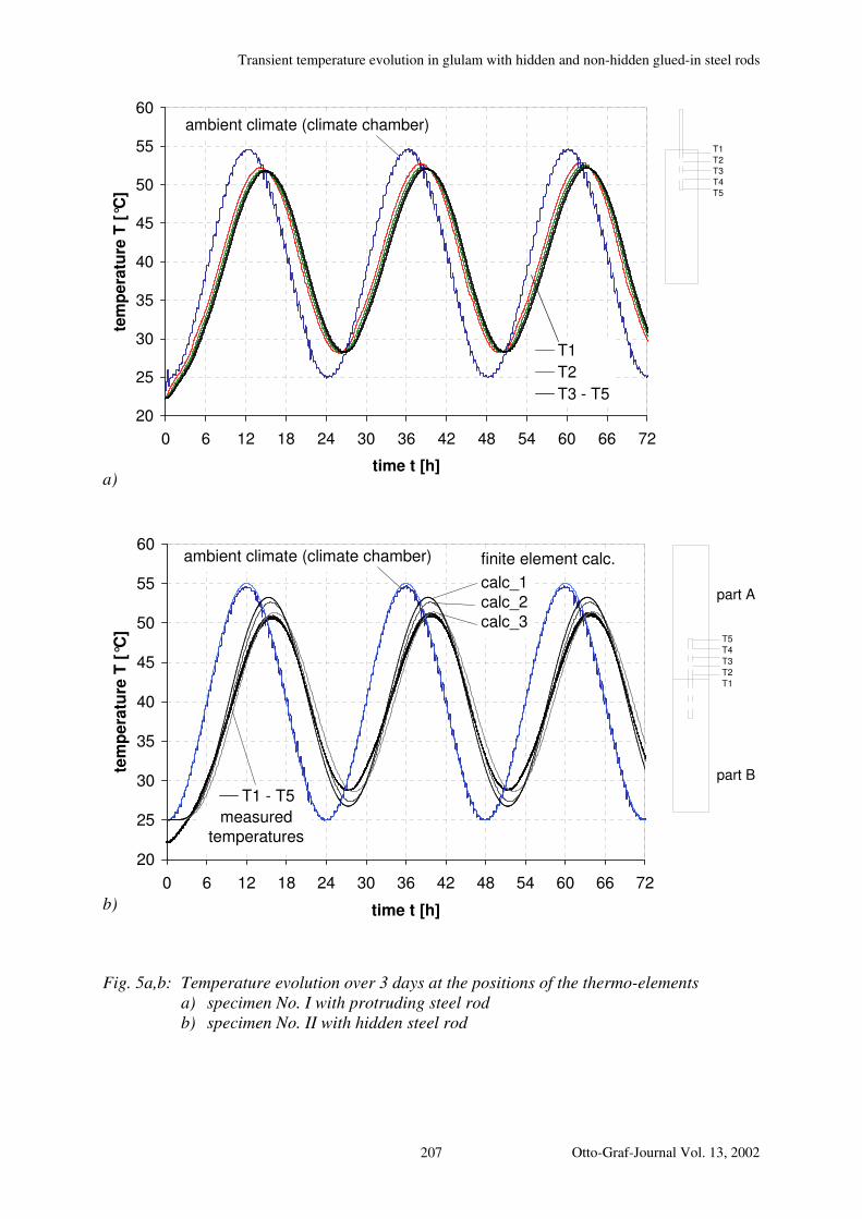
Transient temperature evolution in glulam with hidden and non-hidden glued-in steel rods
a)
20
25
30
35
40
45
50
55
60
0 6 12 18 24 30 36 42 48 54 60 66 72
time t [h]
tem
pera
ture
T [
°C]
T1
T2
T3 - T5
T0T1T2
T4T3
ambient climate (climate chamber)
T1
T2
T3
T4
T5
20
25
30
35
40
45
50
55
60
0 6 12 18 24 30 36 42 48 54 60 66 72
time t [h]
T1 - T5
T
TTTT
ambient climate (climate chamber) finite element calc.
measured temperatures
calc_1calc_2calc_3
T5
T4
T3
T2
T1
part B
part A
[°C
]
tem
pera
ture
T
b)
Fig. 5a,b: Temperature evolution over 3 days at the positions of the thermo-elements a) specimen No. I with protruding steel rod b) specimen No. II with hidden steel rod
Otto-Graf-Journal Vol. 13, 2002 207
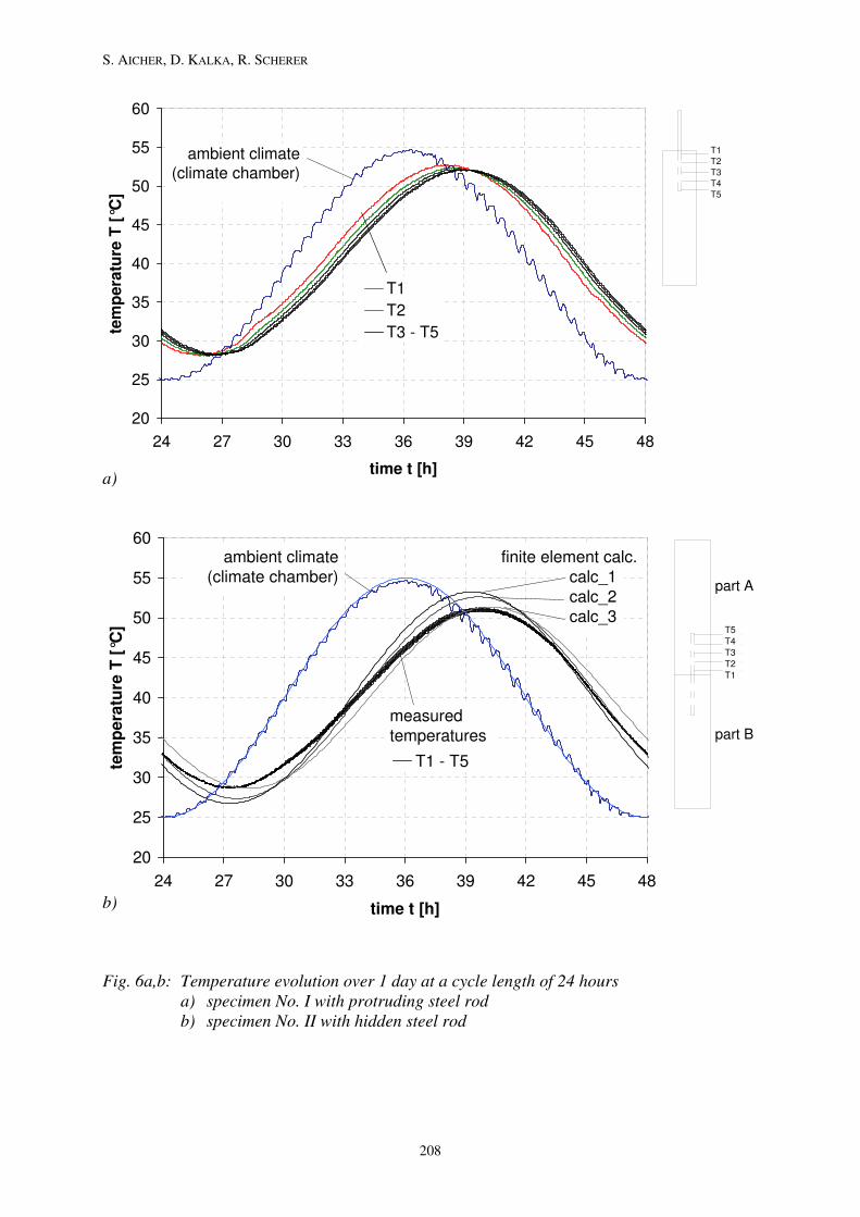
S. AICHER, D. KALKA, R. SCHERER
a)
20
25
30
35
40
45
50
55
60
24 27 30 33 36 39 42 45 48
time t [h]
tem
pera
ture
T [
°C]
T1
T2
T3 - T5
T0T1T2
T4T3
ambient climate (climate chamber)
T1
T2
T3
T4
T5
20
25
30
35
40
45
50
55
60
24 27 30 33 36 39 42 45 48
time t [h]
T1 - T5
ambient climate(climate chamber)
finite element calc.
measured temperatures
calc_1calc_2calc_3
T5
T4
T3
T2
T1
part B
part A
[°C
]
ure
T
tem
pera
t
b)
Fig. 6a,b: Temperature evolution over 1 day at a cycle length of 24 hours a) specimen No. I with protruding steel rod b) specimen No. II with hidden steel rod
208

Transient temperature evolution in glulam with hidden and non-hidden glued-in steel rods
The differences between the two specimen types are rather small. Purely
qualitatively the temperature in the wood-bond line interface of specimen No. II
shows slightly decreased amplitudes and a slightly more pronounced phase shift
vs. ambient climate when compared to specimen No. I with the protruding rod.
Quantitatively the results are specified in Tab. 1.
Tab. 1: Temperature evolution in the wood-adhesive interface of specimens No. I and No. II at thermo-element positions T1 and T5
thermo-element T1
(“protruding” end of steel rod) thermo-element T5
(embedded end of steel rod)
maximum tempera-
ture Tmax
minimum tempera-
ture Tmin
peak-to-peak
amplitude
∆T
phase shift
∆t
maximum tempera-
ture Tmax
minimum tempera-
ture Tmin
peak-to-peak
amplitude
∆T
phase shift
∆t
[°C] [°C] [K] [h] [°C] [°C] [K] [h]
ambient climate
54.7 24.9 29.8 - 54.7 24.9 29.8 -
experimental results:
specimen
No. I (protrud-ing rod)
53.4 28.1 25.3 1.7 52.6 28.2 24.4 2.4
specimen
No. II (hidden rod)
51.2 28.7 22.5 3.3 51.6 28.8 22.8 3.2
It can be seen that the maximum temperatures at the embedded ends of the
rods (thermo-element T5 for specimens No. I and No. II) differ only very little
by about 1°C. The reduction of maximum temperature vs. ambient climate in
case of specimen No. II (hidden rod) was only 3 K. The phase shift between the
maximum temperature of the ambient climate and the maximum of recorded
temperatures was 2.4 and 3.2 hours in case of specimens No. I and No. II, re-
spectively.
In case of specimen No. II no difference of temperature amplitudes, peak
temperatures and phase shifts between thermo-element T1 close to the sealed
joint of both specimen parts A and B as compared to the embedded end (thermo-
element T5) was observed. In case of leakages at the sealing of the joint of the
Otto-Graf-Journal Vol. 13, 2002 209
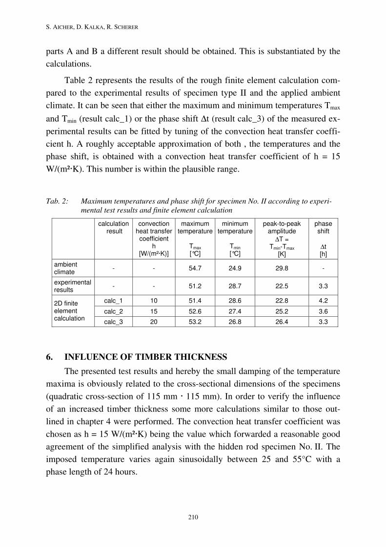
S. AICHER, D. KALKA, R. SCHERER
parts A and B a different result should be obtained. This is substantiated by the
calculations.
Table 2 represents the results of the rough finite element calculation com-
pared to the experimental results of specimen type II and the applied ambient
climate. It can be seen that either the maximum and minimum temperatures Tmax
and Tmin (result calc_1) or the phase shift ∆t (result calc_3) of the measured ex-
perimental results can be fitted by tuning of the convection heat transfer coeffi-
cient h. A roughly acceptable approximation of both , the temperatures and the
phase shift, is obtained with a convection heat transfer coefficient of h = 15
W/(m²·K). This number is within the plausible range.
Tab. 2: Maximum temperatures and phase shift for specimen No. II according to experi-mental test results and finite element calculation
calculation result
convection heat transfer
coefficient h
[W/(m²·K)]
maximum temperature
Tmax
[°C]
minimum temperature
Tmin
[°C]
peak-to-peak amplitude
∆T = Tmin-Tmax
[K]
phase shift
∆t [h]
ambient climate
- - 54.7 24.9 29.8 -
experimental results
- - 51.2 28.7 22.5 3.3
calc_1 10 51.4 28.6 22.8 4.2
calc_2 15 52.6 27.4 25.2 3.6
2D finite element calculation
calc_3 20 53.2 26.8 26.4 3.3
6. INFLUENCE OF TIMBER THICKNESS
The presented test results and hereby the small damping of the temperature
maxima is obviously related to the cross-sectional dimensions of the specimens
(quadratic cross-section of 115 mm · 115 mm). In order to verify the influence
of an increased timber thickness some more calculations similar to those out-
lined in chapter 4 were performed. The convection heat transfer coefficient was
chosen as h = 15 W/(m²·K) being the value which forwarded a reasonable good
agreement of the simplified analysis with the hidden rod specimen No. II. The
imposed temperature varies again sinusoidally between 25 and 55°C with a
phase length of 24 hours.
210

Transient temperature evolution in glulam with hidden and non-hidden glued-in steel rods
Fig. 7 gives the temperature courses for square cross-sectional dimensions
with thicknesses of a = 50, 102, 150 and 200 mm. The value a = 102 mm relates
to the discussed results of specimen No. II, whereby the reduction of the real
thickness of 115 mm to 102 mm is bound to the simplified approach of omitted
rod cross-section. The graph shows the qualitatively somewhat trivial result of a
decreasing temperature amplitude and an increasing phase shift with growing
cross-sectional dimensions.
20
25
30
35
40
45
50
55
60
24 27 30 33 36 39 42 45 48
time t [h]
tem
pera
ture
T [
°C]
T1 - T5
ambient climate(climate chamber)
finite element calc.a = 50, 102, 150, 200 mm
measuredtemperatures
a
T5
T4
T3
T2
T1
Fig. 7: Temperature evolution at a cycle length of 24 hours for finite element calculations with varying timber thicknesses compared to experimental results (specimen No. II with hidden rod)
A quantitative summary of the results is given in Tab. 3. In detail the
changes of minimum and maximum temperature, the peak-to-peak amplitude
∆T = Tmax-Tmin and the phase shift ∆t are specified. It can be seen that the reduc-
tion of the maximum temperature in the regarded range of cross-sectional di-
mensions is rather moderate. For a medium sized glulam thickness of 150 mm
the maximum value is still rather close to 50°C, which marks the limit of type I
adhesives acc. to EN 301.
The quantitative results of the very rough approximation of the problem
shall be regarded with a more refined modeling considering the true build-ups.
Otto-Graf-Journal Vol. 13, 2002 211
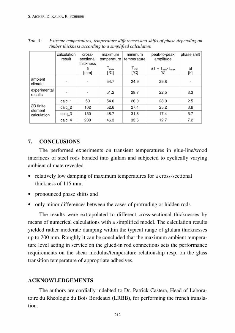
S. AICHER, D. KALKA, R. SCHERER
Tab. 3: Extreme temperatures, temperature differences and shifts of phase depending on timber thickness according to a simplified calculation
calculation result
cross-sectional thickness
a [mm]
maximum temperature
Tmax
[°C]
minimum temperature
Tmin
[°C]
peak-to-peak amplitude
∆T = Tmin-Tmax [K]
phase shift
∆t [h]
ambient climate
- - 54.7 24.9 29.8 -
experimental results
- - 51.2 28.7 22.5 3.3
calc_1 50 54.0 26.0 28.0 2.5
calc_2 102 52.6 27.4 25.2 3.6
calc_3 150 48.7 31.3 17.4 5.7
2D finite element calculation
calc_4 200 46.3 33.6 12.7 7.2
7. CONCLUSIONS
The performed experiments on transient temperatures in glue-line/wood
interfaces of steel rods bonded into glulam and subjected to cyclically varying
ambient climate revealed
• relatively low damping of maximum temperatures for a cross-sectional
thickness of 115 mm,
• pronounced phase shifts and
• only minor differences between the cases of protruding or hidden rods.
The results were extrapolated to different cross-sectional thicknesses by
means of numerical calculations with a simplified model. The calculation results
yielded rather moderate damping within the typical range of glulam thicknesses
up to 200 mm. Roughly it can be concluded that the maximum ambient tempera-
ture level acting in service on the glued-in rod connections sets the performance
requirements on the shear modulus/temperature relationship resp. on the glass
transition temperature of appropriate adhesives.
ACKNOWLEDGEMENTS
The authors are cordially indebted to Dr. Patrick Castera, Head of Labora-
toire du Rheologie du Bois Bordeaux (LRBB), for performing the french transla-
tion.
212

Transient temperature evolution in glulam with hidden and non-hidden glued-in steel rods
REFERENCES
AICHER, S. (2002): Duration of load tests on full-sized glued-in rod specimens.
GIROD_WP5: Technical Report for work package 5, Research Report,
Otto-Graf-Institute, University of Stuttgart.
AICHER, S.; KALKA, D.; HÖFFLIN, L. (2001): Duration of load tests on full-
sized glued-in rod specimens. GIROD_WP5: Technical Report for work
package 5, workpart by FMPA. Research Report, Otto-Graf-Institute,
University of Stuttgart.
AICHER, S.; WOLF, M.; DILL-LANGER, G. (1998): Heat flow in a glulam joist
with a glued-in steel rod subjected to variable ambient temperature.
Otto-Graf-Journal Vol. 9, pp. 185-204 , Otto-Graf-Institute, University of
Stuttgart.
BATZER, H. (1985): Polymere Werkstoffe. Volume I, Georg Thieme Verlag
Stuttgart. New York.
BENGTSSON, C.; JOHANSSON, C.-J. (2002): GIROD – Glued in rods for timber
structures. SP Report 2002:26. SP Swedish National Testing and Research
Institute.
Otto-Graf-Journal Vol. 13, 2002 213

S. AICHER, D. KALKA, R. SCHERER
214

Modelling of concrete hydration
MODELLING OF CONCRETE HYDRATION
MODELLIERUNG DER BETON HYDRATATION
MODELISATION DE L'HYDRATATION DU BETON
Sven Mönnig
SUMMARY
DuCOM is a finite element program which can show the hydration of
concrete with any concrete mixtures, to any given time step and different
environmental conditions. Comparing calculated temperature distribution,
hydration and heat growth rates with measurements a high accuracy was proven.
ZUSAMMENFASSUNG
DuCOM ist ein FEM-Programm, welches die Hydratation von Beton mit
beliebigen Betonmischungen, zu beliebigen Zeitschritten und verschiedenen
Umgebungsbedingungen darstellen kann. Bei dem Vergleich von errechneten
Temperaturverläufen, Hydratationskurven und Wärmezuwachsraten mit
gemessenen Laborwerten, zeigt sich eine hohe Genauigkeit von DuCOM.
RÉSUMÉ
DuCOM est un programme d'éléments finis capable de décrire l'hydratation
de bétons de compositions arbitraires, à des intervalles arbitraires et pour
différentes conditions d'environnement. La comparaison des gradients de
température, des courbes d'hydratation et des taux de chaleur calculés avec les
valeurs mesurées en laboratoire indiquent une précision élevée de DuCOM.
KEYWORDS: DuCOM, heat growth rate, concrete hydration
1. INTRODUCTION
DuCOM [1] is a program working with concrete finite elements. It is able
to deliver a linear description of the hydration of concrete. It provides solutions
for pore pressure and temperature at each node of each element for given time
steps and environmental condition, i.e. relative humidity and temperature.
Otto-Graf-Journal Vol. 13, 2002 215
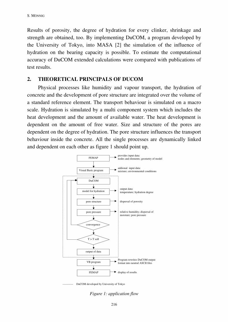
S. MÖNNIG
Results of porosity, the degree of hydration for every clinker, shrinkage and
strength are obtained, too. By implementing DuCOM, a program developed by
the University of Tokyo, into MASA [2] the simulation of the influence of
hydration on the bearing capacity is possible. To estimate the computational
accuracy of DuCOM extended calculations were compared with publications of
test results.
2. THEORETICAL PRINCIPALS OF DUCOM
Physical processes like humidity and vapour transport, the hydration of
concrete and the development of pore structure are integrated over the volume of
a standard reference element. The transport behaviour is simulated on a macro
scale. Hydration is simulated by a multi component system which includes the
heat development and the amount of available water. The heat development is
dependent on the amount of free water. Size and structure of the pores are
dependent on the degree of hydration. The pore structure influences the transport
behaviour inside the concrete. All the single processes are dynamically linked
and dependent on each other as figure 1 should point up.
FEMAP
Visual Basic program
provides input data: nodes and elements; geometry of model
addional input data: mixture; environmental conditions
DuCOM
model for hydration
pore structure
pore pressure
convergence
T > T soll
output of data
VB program Program rewrites DuCOM output format into neutral ASCII files
FEMAP display of results
DuCOM developed by University of Tokyo
output data: temperature; hydration degree
dispersal of porosity
relative humidity; dispersal of moisture; pore pressure
Figure 1: application flow
216
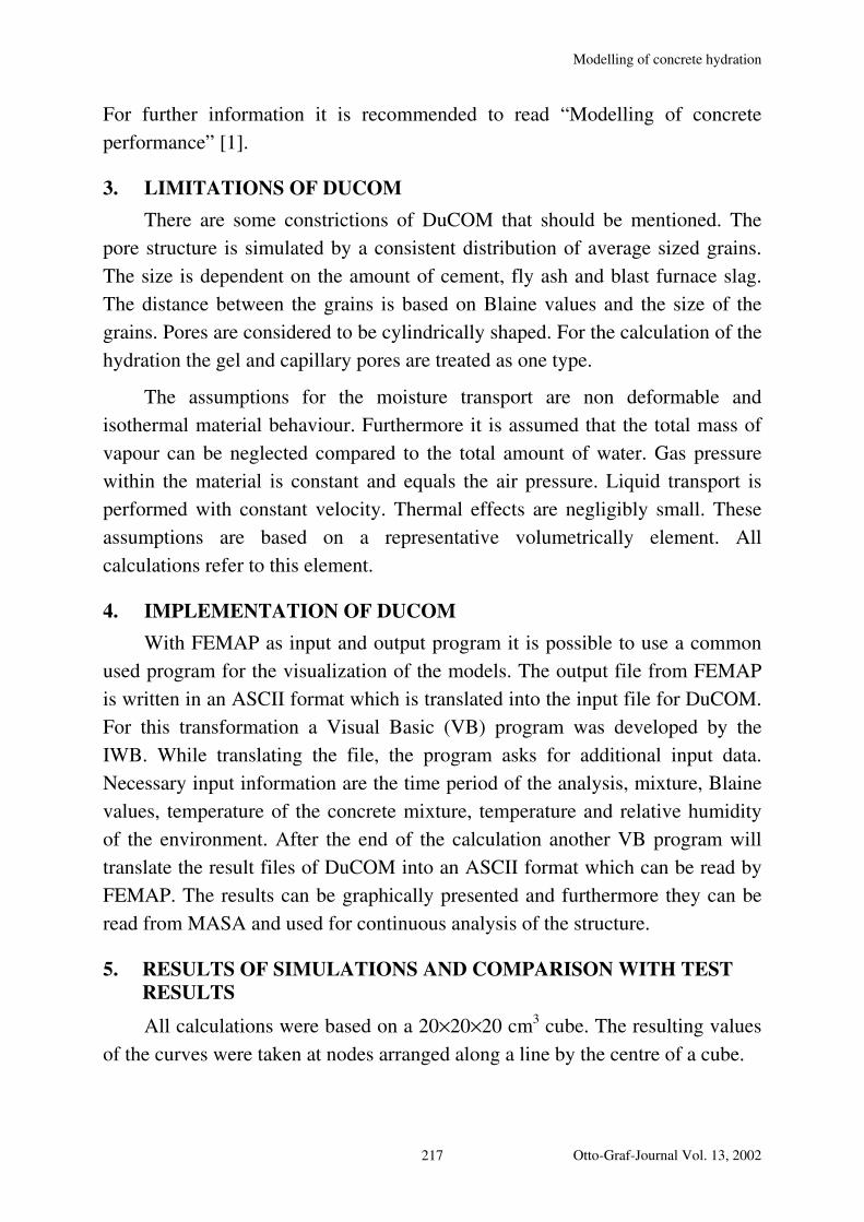
Modelling of concrete hydration
For further information it is recommended to read “Modelling of concrete
performance” [1].
3. LIMITATIONS OF DUCOM
There are some constrictions of DuCOM that should be mentioned. The
pore structure is simulated by a consistent distribution of average sized grains.
The size is dependent on the amount of cement, fly ash and blast furnace slag.
The distance between the grains is based on Blaine values and the size of the
grains. Pores are considered to be cylindrically shaped. For the calculation of the
hydration the gel and capillary pores are treated as one type.
The assumptions for the moisture transport are non deformable and
isothermal material behaviour. Furthermore it is assumed that the total mass of
vapour can be neglected compared to the total amount of water. Gas pressure
within the material is constant and equals the air pressure. Liquid transport is
performed with constant velocity. Thermal effects are negligibly small. These
assumptions are based on a representative volumetrically element. All
calculations refer to this element.
4. IMPLEMENTATION OF DUCOM
With FEMAP as input and output program it is possible to use a common
used program for the visualization of the models. The output file from FEMAP
is written in an ASCII format which is translated into the input file for DuCOM.
For this transformation a Visual Basic (VB) program was developed by the
IWB. While translating the file, the program asks for additional input data.
Necessary input information are the time period of the analysis, mixture, Blaine
values, temperature of the concrete mixture, temperature and relative humidity
of the environment. After the end of the calculation another VB program will
translate the result files of DuCOM into an ASCII format which can be read by
FEMAP. The results can be graphically presented and furthermore they can be
read from MASA and used for continuous analysis of the structure.
5. RESULTS OF SIMULATIONS AND COMPARISON WITH TEST RESULTS
All calculations were based on a 20×20×20 cm3 cube. The resulting values
of the curves were taken at nodes arranged along a line by the centre of a cube.
Otto-Graf-Journal Vol. 13, 2002 217
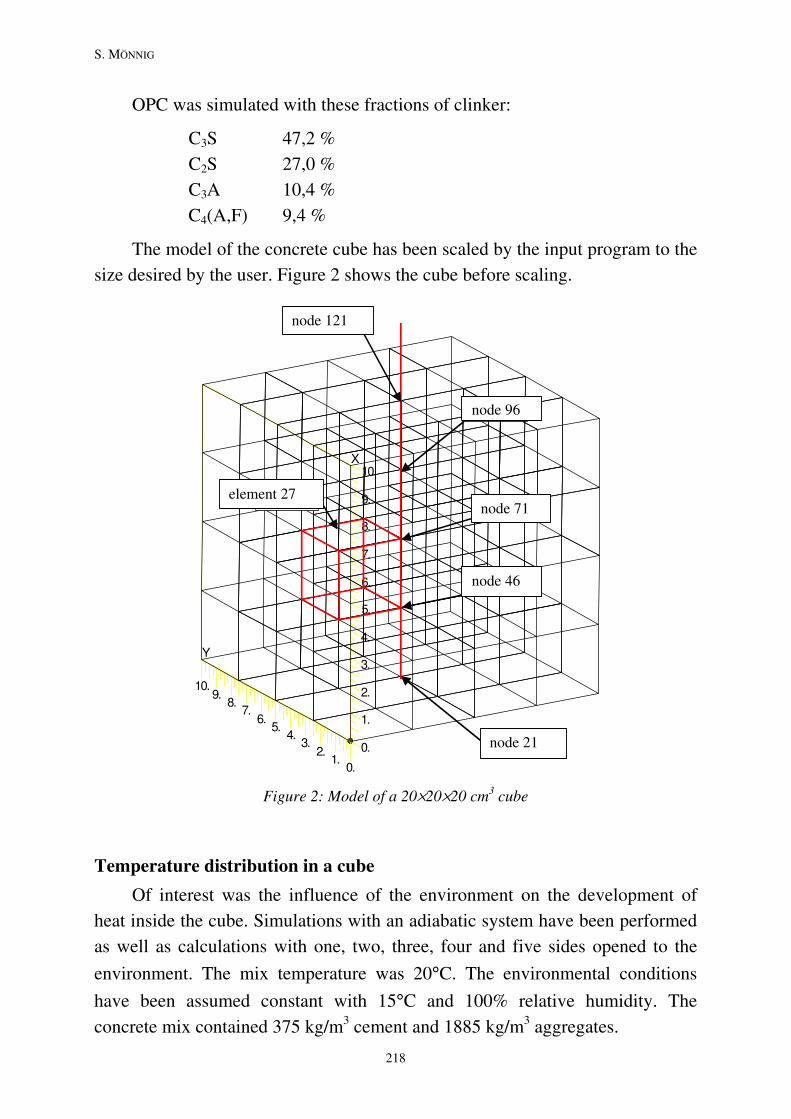
S. MÖNNIG
OPC was simulated with these fractions of clinker:
C3S 47,2 %
C2S 27,0 %
C3A 10,4 %
C4(A,F) 9,4 %
The model of the concrete cube has been scaled by the input program to the
size desired by the user. Figure 2 shows the cube before scaling.
X
0.
1.
2.
3.
4.
5.
6.
7.
8.
9.
10.
Y
0.1.
2.3.
4.5.
6.7.
8.9.
10.
Knoten 121
Knoten 96
Knoten 71
Knoten 46
Knoten 21
Element 27
node 121
node 96
node 71
node 46
node 21
element 27
Figure 2: Model of a 20×20×20 cm3 cube
Temperature distribution in a cube
Of interest was the influence of the environment on the development of
heat inside the cube. Simulations with an adiabatic system have been performed
as well as calculations with one, two, three, four and five sides opened to the
environment. The mix temperature was 20°C. The environmental conditions
have been assumed constant with 15°C and 100% relative humidity. The
concrete mix contained 375 kg/m3 cement and 1885 kg/m3 aggregates.
218

Modelling of concrete hydration
0.00 0.01 0.10 1.00 10.00 100.00
Figure 3: Temperature distribution inside a cube
Degree of Hydration in dependence on the water/cement ratio
The proportion has been changed to a mixture with very high cement
content. It contained 836.3 kg/m3 cement and 1032 kg/m3 aggregates. These
fractions have been chosen to minimize the influence of the aggregates on the
water diffusion and the hydration. The reference mixture had a water/cement
ratio of 0.4 but the same cement and aggregate content as the others. This
mixture has been calculated with five sides open to the environment which had a
constant temperature of 15°C and a relative humidity of 100 %.
Progress of hydration
0,0
0,1
0,2
0,3
0,4
0,5
0,6
0,7
0,8
0,9
1,0
0 4 8 12 16 20 24
Hours [h]
Hyd
rati
on
Deg
ree [
%]
W/C 0.4 Five Open
Sides
W/C 0.20 Adiabatic
W/C 0.40 Adiabatic
W/C 0.60 Adiabatic
1.0
0.9
0.8
0.7
0.6
0.5
0.4
0.3
0.2
0.1
0.0
Figure 4: Degree of hydration in dependence on the water/cement ratio
Otto-Graf-Journal Vol. 13, 2002 219
S. MÖNNIG
Heat growth rate of clinker
DuCOM provides the overall generated heat for each clinker at each time
step. By subtracting the accumulated heat at one time step from the previous one
it was possible to calculate the heat growth rate. The curves presented in figure 5
have been interpolated with Excel to abrade them. DuCOM calculated 2500 time
steps to reach 24 hours.
0,00
0,05
0,10
0,15
0,20
0,25
0,30
0 4 8 12 16 20 24
Time [h]
He
at
Gro
wth
Ra
te [
kc
al/k
g]
C3A
C3S
C4AF
C2S
Total Heat
0.30
0.25
0.20
0.15
0.10
0.00
0.05
Figure 5: Heat growth rate of clinker
6. DISCUSSION
The maximum temperature of the hydration as shown in figure 3 does
reach the extent as expected. Different methods of gaining an approximated
value do provide similar results, e.g. the approximation formula for adiabatic
heat growth as given in [3] provides likewise results. The results presented in
figure 5 follow the expected curves. The influence of the low temperature of the
environment on the rate of hydration is reasonable, too. The curves in figure 5
show the same behaviour of the clinker as it was expected due to the specific
enthalpy of each clinker.
7. SUMMARY OF RESULTS
DuCOM proved to be very reliable being used for the simulation of
hydration of ordinary Portland cements and their mixtures. Temperature
development and hydration degree are corresponding with measured values
given in the literature. More calculations and experiments should be performed
to estimate the accuracy of calculated strength and shrinkage.
220

Modelling of concrete hydration
REFERENCES
[1] Maekawa, K.; Chaube R., Kishi, T.: Modelling of concrete performance,
E&FN Spon, London, 1999
[2] Ožbolt, J.: MASA – Macroscopic Space Analysis. Internal Report, Institut
für Werkstoffe im Bauwesen, Universität Stuttgart, 1998
[3] Zement Taschenbuch 2000, Verlag Bau+Technik, Düsseldorf, 2000
Otto-Graf-Journal Vol. 13, 2002 221