correlations in quantum physics

November 5, 2012 9:31 WSPC/Guidelines-IJMPB S0217979213450173

International Journal of Modern Physics BVol. 27, Nos. 1–3 (2013) 1345017 (15 pages)c© World Scientific Publishing Company

DOI: 10.1142/S0217979213450173

CORRELATIONS IN QUANTUM PHYSICS

ROSS DORNER

Blackett Laboratory, Imperial College London, Prince Consort Road,

London SW7 2AZ, UK

Clarendon Laboratory, University of Oxford, Parks Road,

Oxford OX1 3PU, UK

VLATKO VEDRAL

Clarendon Laboratory, University of Oxford, Parks Road,

Oxford OX1 3PU, UK

Centre for Quantum Technologies, National University of Singapore,

3 Science Drive 2, 117543, Singapore

Department of Physics, National University of Singapore,

2 Science Drive 3, 117542, Singapore

Received 10 August 2012Accepted 15 August 2012

Published 8 November 2012

We provide a historical perspective of how the notion of correlations has evolved withinquantum physics. We begin by reviewing Shannon’s information theory and its first ap-plication in quantum physics, due to Everett, in explaining the information conveyedduring a quantum measurement. This naturally leads us to Lindblad’s information the-oretic analysis of quantum measurements and his emphasis of the difference between

the classical and quantum mutual information. After briefly summarizing the quantifi-cation of entanglement using these ideas, we arrive at the concept of quantum discord,which naturally captures the boundary between entanglement and classical correlations.Finally we discuss possible links between discord, which the generation of correlationsin thermodynamic transformations of coupled harmonic oscillators.

Keywords: Quantum correlations; quantum nonequilibrium thermodynamics.

1. Introduction

Correlations play a prominent role in many-body physics, statistical physics and

information technology. Here, however, we focus on another motivation for studying

correlations, namely that they offer the best way of understanding the key differ-

ences between quantum and classical physics. Quantum mechanics allows for the

full range of correlations between events. For instance, there is a maximal corre-

lation between earlier and later states of quantum systems undergoing a unitary

1345017-1

Int.

J. M

od. P

hys.

B 2

013.

27. D

ownl

oade

d fr

om w

ww

.wor

ldsc

ient

ific

.com

by M

AR

SHA

LL

UN

IVE

RSI

TY

on

08/2

0/13

. For

per

sona

l use

onl

y.

http://dx.doi.org/10.1142/S0217979213450173


R. Dorner & V. Vedral

evolution. At the other extreme are completely uncorrelated quantum events, such

as measuring a spin half particle successively in two complementary bases. All other

partial degrees of correlation, between maximal and zero, are also found in quantum

physics.

In this paper, we will recap how information theory can be used to quantify

correlations in general. We then show how this was applied by Everett and Lind-

blad to elucidate the quantum measurement process. This is followed by a brief

summary of the two main types of quantum correlation, entanglement and quan-

tum discord. Finally, the role of correlations is explored in the field of quantum

thermodynamics by investigating the link between correlations and the amount of

work in tranforming two couple harmonic oscillators.

2. Shannon’s Information Theory

Given two random variables, X with the set of possible outcomes xi and Y

with the set of possible outcomes yj, we define the joint probability distribution

P (X = xi, Y = yj) ≡ p(xi, yj) with corresponding marginal probability distribu-

tions P (A = ai) ≡ p(xi) =∑

j p(xi, yj) and P (Y = yj) ≡ p(yj) =∑

i p(xi, yj).

The degree of correlation between the random variable X and Y is encoded in

their joint probability distribution and best quantified within the framework of

Shannon’s information theory.1 We therefore begin our discussion by defining the

Shannon entropy of the random variable X , as

S(X) ≡ S(p(x)) = −∑

i

p(xi) ln p(xi) (1)

and analogously S(Y ) = −∑

j p(yj) ln p(yj). As is well known, the Shannon entropy

provides a measure of the uncertainty in a given random variable. By straightfor-

ward generalization of Eq. (1) we also define the uncertainty in the joint distribution

of X and Y is defined by

S(X,Y ) ≡ S(p(x, y)) = −∑

i,j

p(xi, yj) ln p(xi, yj) .

From this, we are able to define the Shannon mutual information,

IS(X : Y ) = S(p(x)) + S(p(y))− S(p(x, y)) . (2)

This quantity, being positive, provides an intuitive interpretation of correlation

between X and Y . Explicitly, it states that the sum of the uncertainties in p(x) and

p(y) alone is greater than the uncertainty in their joint distribution p(x, y). Next,

we introduce the Shannon relative entropy,

S(X‖Y ) ≡ S(p(x)‖p(y)) =∑

i,j

p(xi) lnp(xi)

p(yj),

allowing the Shannon mutual information Eq. (2) to be rewritten as

IS(A : B) = S(

p(x, y)‖p(x)× p(y))

.

1345017-2

Int.

J. M

od. P

hys.

B 2

013.

27. D

ownl

oade

d fr

om w

ww

.wor

ldsc

ient

ific

.com

by M

AR

SHA

LL

UN

IVE

RSI

TY

on

08/2

0/13

. For

per

sona

l use

onl

y.


Correlations in Quantum Physics

In this sense, the mutual information represents a distance between the joint prob-

ability distribution p(x, y) and the product of its marginals p(x)× p(y). As such, it

is intuitively clear that IS is a good measure of correlations, since it shows how far

a joint distribution is from the corresponding product distribution in which all the

correlations have been destroyed. We can also view the Shannon mtual information

from a third perspective. Suppose that we wish to know the probability of observing

the event yj given that the event xi has been observed. The relevant quantity is

the conditional probability, given by

P (Y = yj |X = xi) ≡ pxi(yj) =

p(xi, yj)

p(xi).

This motivates us to introduce the conditional entropy, SX(Y ), as

SX(Y ) = −∑

i

p(xi)∑

j

pxi(yj) ln pxi

(yj)

= −∑

i,j

p(xi, yj) ln pxi(yj) .

The conditional entropy tells us how uncertain we are about the value of Y once

we have learned the value of X . The Shannon mutual information Eq. (2) can now

be rewritten once more as

IS(X : Y ) = S(Y )− SX(Y ) = S(X)− SY (X) . (3)

Thus, as its name indicates, the Shannon mutual information measures the quantity

of information conveyed about the random variable X (Y ) through measurements

of the random variable Y (X). As this quantity is positive, it tells us that the

initial uncertainty in Y (X) can in no way be increased by making observations on

X (Y ). Note also that, unlike the Shannon relative entropy, the Shannon mutual

information is symmetric i.e., IS(X : Y ) = IS(Y : X).

Shannon’s original motivation for developing this framework was the practical

need of quantifying the channel capacity of classical communication channels. In this

scenario, X and Y represent the message sent down and received from the channel,

respectively. Given that process of measurement can be viewed as a communication

channel between the states of the system and the observer, it was only natural that

Everett would use Shannon’s information theory to characterize quantum measure-

ments within his relative state interpretation of quantum physics.2 The novelty of

Everett’s approach was the discussion of information in quantum measurements

without recourse to the Born projection postulate. Everett did not discriminate

between quantum and classical correlations, though he implicitly worked only with

classical correlations as we now understand them.

3. Everett’s View of Correlations

According to the relative state view of quantum physics, a quantum measure-

ment never gives conclusive results, but instead establishes correlations between

1345017-3

Int.

J. M

od. P

hys.

B 2

013.

27. D

ownl

oade

d fr

om w

ww

.wor

ldsc

ient

ific

.com

by M

AR

SHA

LL

UN

IVE

RSI

TY

on

08/2

0/13

. For

per

sona

l use

onl

y.



the system and the measuring device. As an example, consider a system consisting

of a single qubit. The typical Everettian style measurement takes initially uncorre-

lated states of the system and measuring device to the post-measurement, correlated

state

|ψAB〉 = α|0〉|m1〉+ β|1〉|m2〉 , (4)

where |0〉 and |1〉 are orthogonal states of the system, |m1〉 and |m2〉 are states of themeasuring device with overlap 〈b0|b1〉 = ǫ and |α|2+ |β|2 = 1. Intuitively, the degree

of correlation between the system and measurement device depends upon ǫ. This

intuition can be quantified within the framework of Shannon’s information theory

by first introducing one observable pertaining to the system X = x1|x1〉〈x1| +x2|x2〉〈x2|, and one observable pertaining to the measuring device Y = y1|y1〉〈y1|+y2|y2〉〈y2|. The outcomes of measurements of these observables give rise to the two

probability distributions, p(xi) = |〈ψAB |xi〉|2 and p(yj) = |〈ψAB |yj〉|2 as well as thejoint distribution p(xi, yj) = |〈ψAB|xi〉|yj〉|2. We can now quantify the uncertainty

in the observable X and Y via the Shannon entropy Eq. (1) and their correlation

via the Shannon mutual information Eq. (2). At this point, we make the important

remark that while Everett showed that Shannon’s information theory is capable of

quantifying some correlations in quantum theory, it does not tell us the whole story.

The correlation in post measurement quantum state itself Eq. (4), for instance, must

be quantified using the quantum generalization of Shannon’s information theory.

This will be the focus of Secs. 4–6.

Everett went on to establish the properties that must be possessed by any

“good” measure of correlations between two random variables. Namely, he proved

that if either or both of the variables undergo a local stochastic evolution, then the

amount of correlations between them cannot increase (in fact it usually decreases,

see also Ref. 3). As far as quantum measurements are concerned, this describes the

physically intuitive fact that correlations established during the quantum measure-

ments cannot be increased, i.e., the measurement cannot be made to yield more

information, by further processing the system and the apparatus separately. We

note however, that when local stochastic processes are correlated they virtually

become global, and therefore the correlations between the systems can increase as

well as decrease. A generalization of this logic is central to the theory of quanti-

fying quantum correlations under the paradigm of local operations and classical

communication (LOCC), which will return to in Sec. 5. Next, however, we discuss

another important step in the development of correlations in quantum physics, due

to Lindblad.

4. Lindblad’s Analysis of Quantum Measurements

Lindblad built on Everett’s initial work by generalizing his theory of quantum mea-

surements to encompass mixed states in contact with an environment.4 In doing

so, Lindblad employed the quantum versions of many quantities from Shannon’s

1345017-4

Int.

J. M

od. P

hys.

B 2

013.

27. D

ownl

oade

d fr

om w

ww

.wor

ldsc

ient

ific

.com

by M

AR

SHA

LL

UN

IVE

RSI

TY

on

08/2

0/13

. For

per

sona

l use

onl

y.



information theory. The formulation of classical probability theory that is most

naturally generalized to quantum states is provided by Kolmogorov,5 and an expo-

sition expressing similarities with von Neumann’s Hilbert Space formulation6 due

to Mackey7 (see also Ref. 8). For our purposes, however, it suffices to introduce the

relevant quantities ad hoc by straightforward analogy with their classical counter-

parts.

First, for a quantum system described by a density matrix ρ, we define its von

Neumann entropy as

SN (ρ) = −Tr[ρ ln ρ] . (5)

This can be considered as the proper quantum analogue of the Shannon entropy

Eq. (1).9–11 For an observable A of the system described by ρ, the Shannon entropy

S(A), describing the uncertainties in the values of the observables, is equal to the

von Neumann entropy SN (ρ) only when [A, ρ] = 0 i.e., A is a Schmidt observable.

Otherwise,

S(A) ≥ SN (ρ) .

The physical interpretation of this result is that there is more uncertainty in a

single observable than in the whole of the state, a fact which entirely contradicts

our expectations from the earlier, classical discussion.

The concept of mutual information Eq. (2) can also be easily extended to

quantum systems.12 For a bipartite state ρAB and corresponding reduced states

ρA = TrB[ρAB] and ρB = TrA[ρAB], we define the von Neumann mutual informa-

tion between the two subsystems as

IN (ρA : ρB; ρAB) = SN (ρA) + SN (ρB)− SN (ρAB) . (6)

Note that this quantity describes the correlation between the whole subsystems

rather than relating two observables only. Following the Shannon mutual informa-

tion, this quantity can be interpreted as a distance between two quantum states by

introducing the von Neumann relative entropy, (in fact, this quantity was first con-

sidered by Umegaki,13 but for consistency reasons we name it after von Neumann).

The von Neumann relative entropy between two quantum states σ and ρ is defined

as

SN (σ‖ρ) = Tr[σ(lnσ − ln ρ)] . (7)

The von Neumann mutual information Eq. (6) can now be understood as a distance

of the state ρAB to the uncorrelated state ρA ⊗ ρB,

IN (ρA : ρB ; ρAB) = SN (ρAB‖ρA ⊗ ρB) . (8)

Lindblad’s main contribution was to calculate and compare the classical and quan-

tum mutual information during a measurement. This analysis was motivated by

thermodynamical considerations. A question he considered is how much entropy is

generated during a quantum measurement. The entropy increase is fundamentally

1345017-5

Int.

J. M

od. P

hys.

B 2

013.

27. D

ownl

oade

d fr

om w

ww

.wor

ldsc

ient

ific

.com

by M

AR

SHA

LL

UN

IVE

RSI

TY

on

08/2

0/13

. For

per

sona

l use

onl

y.



linked with the irreversibility of the quantum measurement and the correlations

created between the system and an apparatus. We will return to the connection

between correlations and thermodynamics in Sec. 7.

We now discuss a relation concerning the entropies of two subsystems; the

Araki–Lieb inequality.14

SN (ρA) + SN (ρB) ≥ SN(ρ) ≥ |SN (ρA)− SN(ρB)| . (9)

This can be considered one of the most important results in the quantum theory of

correlations. Physically, Eq. (9) implies that there is more information (less uncer-

tainty) in an entangled state than if the two states are treated separately. On the

one hand, this arises naturally from considering the subsystems separately and ne-

glecting the correlations between them. However, to appreciate the extent to which

this is a counter-intuitive result, consider a two level atom interacting with a single

mode of an EM field, as in the Jaynes–Cummings model.15 If the overall state is

initially pure, and the whole system is isolated, then the entropies of the atom and

the field are equally uncertain at all the times. This observation is surprising given

that the atom has only two degrees of freedom and the field has infinitely many.

Crucially, however, the two level atom is only ever entangled with two dimensions

of the field.

5. Quantifying Entanglement

The global state of a composite system is entangled if it may not be written as a

product of the individual subsystems.16–18 This implies that though the global state

of the composite system may be known with certainty, the state of each individual

subsystem is uncertain, or, as Schrodinger put it, “The best possible knowledge of

a whole does not include the best possible knowledge of its parts”19 [c.f. Eq. (9)].

This reasoning can be quantified by considering the two qubit state

|ΨAB〉 = cosθ

2|0A0B〉+ sin

θ

2|1A1B〉 , (10)

which, following the above definition is entangled for 0 < θ < π. For pure bipartite

states, the amount of entanglement present is uniquely quantified by the von Neu-

mann entropy Eq. (5) of (either of) the subsystems.20 Though the von Neumann

entropy of the global state is zero, that of each of the reduced states is finite and

determined by θ,

SN (ρA) = SN (ρB) = − cos2θ

2ln cos2

θ

2− sin2

θ

2ln sin2

θ

2. (11)

The entanglement is thus the lack of information concerning the reduced states

of the subsystems in light of maximal information regarding the global state.

Conversely, the more entangled the global state is the less information we have

concerning the states of the subsystems.

For a separable state (θ = 0, π), the von Neumann entropy of the global and

reduced states are identically zero. Conversely, when cos(θ/2) = sin(θ/2) = 1/√2,

1345017-6

Int.

J. M

od. P

hys.

B 2

013.

27. D

ownl

oade

d fr

om w

ww

.wor

ldsc

ient

ific

.com

by M

AR

SHA

LL

UN

IVE

RSI

TY

on

08/2

0/13

. For

per

sona

l use

onl

y.



the state Eq. (10) is maximally entangled and its reduced states are maximally

mixed i.e., SN (ρA) = SN (ρB) = ln 2. It follows that the von Neumann mutual

information Eq. (6) of a maximally entangled state IN (ρA; ρB : ρAB) = 2 ln 2, is

twice the maximum possible value of the Shannon mutual information between two

random variables. Lindblad was the first to attribute this stronger-than-classical

correlation to entanglement, though this assertion is only accurate for pure bipartite

states and in general, entanglement does not encapsulate all forms of nonclassical

correlation. Note that for other values of 0 < θ < π, the state is entangled but the

von Neumann mutual information may not exceed the maximum possible Shanon

mutual information.

More generally, for finite dimensional N -partite states, entanglement presents

any form of correlation that cannot be captured by a separable state of the

form

σ =∑

i

p(i)π(i)1 ⊗ · · · ⊗ π

(i)N , (12)

where πn is the reduced density matrix of the Nth subsystem. Operationally speak-

ing, separable states are those that are preparable under the paradigm of LOCC,

while all other states are entangled.21,22 The entanglement in a quantum state can

thus be quantified by its distance to the closest separable state.20,23 This distance

can be expressed in a number of ways but the related details will not trouble us at

present (see e.g., Ref. 24). For infinite dimensional (continuous variable) systems,

the theory of entanglement for the physically relevant set of Gaussian states is also

well developed.25,26

Entanglement aside, there are other forms of correlation in quantum systems

with no counterpart in classical information theory. Just as with entanglement, the

degree of other quantum correlations in a given state may be measured by its closest

distance to other sets of states, which we briefly summarize here.27 First, the set of

classical states have the general form

χ =∑

k1,...,kN

p(k1, . . . , kN )|k1 · · · kN 〉〈k1 · · · kN | . (13)

This simply means that for a bipartite state of subsystem A spanned by the

orthogonal basis |ai〉, and a subsystem B spanned by the orthogonal basis

|bj〉, the state χ =∑

i,j p(ai, bj)|ai〉〈ai| ⊗ |bj〉〈bj | is classically correlated when

one or more of the associated joint probabilities do not factorize as p(ai, bj) =

p(ai)× p(bj).

The states containing zero correlations, either quantum or classical, are the

product states of the form

π = π1 ⊗ · · · ⊗ πN . (14)

Note that the product states are a subset of the classical states which in turn are

a subset of the separable states. The need to discriminate between separable states

1345017-7

Int.

J. M

od. P

hys.

B 2

013.

27. D

ownl

oade

d fr

om w

ww

.wor

ldsc

ient

ific

.com

by M

AR

SHA

LL

UN

IVE

RSI

TY

on

08/2

0/13

. For

per

sona

l use

onl

y.



and classically correlated states follows from the existence of more forms of cor-

relations than just entanglement and classical correlations. This point is discussed

further in the following section.

6. Quantifying Discord

Quantum discord describes all forms of correlations beyond those encapsulated by

classically correlated states. For a system of two qubits, A and B, the amount

discord they share can be quantified using an entropic measure by an extension of

Shannon’s original logic. The more correlated A and B are, the more we can learn

about one by measuring the other. Accordingly, the degree of correlation between A

and B is quantified by the reduction of entropy of A (B) when B (A) is measured.

Measurement of the state of subsystem A is described by a positive oper-

ator value measure (POVM) whose elements Ej satisfy the completeness rela-

tion∑

j Ej = 1. For each measurement outcome j, occurring with probability

pj = tr(EjρAB), the post-measurement state of B is ρ(j)B = trA(EjρAB)/pj . The

total classical correlations in the state ρAB are then simply the maximum over all

possible measurements performed on A of the quantity28–30

C(ρAB) = SN (ρB)−∑

j

pjSN (ρ(j)B ) . (15)

This quantity can be considered as one possible quantum generalization of the

classical mutual information Eq. (3). The classical mutual information can also be

defined by swapping the roles of A and B, but the subtleties related to the question

of symmetry of correlations in this context will not be relevant for our present

discussion. The quantum discord of ρAB is then defined as the difference between

the total correlation in the state, given by the von Neumann mutual information

Eq. (8), and the classical correlations31,32

D(B|A) = I(A : B)−maxEi

[C(ρAB)]

= minEi

[I(A : B)− C(ρAB)] , (16)

where, as previously mentioned, the maximization is performed over all possible

POVMs acting on A.

The discord is thus the difference between two forms of the mutual information

that are equivalent in classical information theory. Hence for classically correlated

states the discord is zero, as expected. The discrepancy between these two quan-

tities in quantum information theory arises from the role of measurement. While,

classically, measurement serves to reveal the objective property of the system, in

quantum mechanics the outcomes of measurement are basis dependent and effect

the state of the system.

More generally, following the discussion of Sec. 5, for a general N -partite state

the discord is quantified by its distance to the closest classically correlated state

1345017-8

Int.

J. M

od. P

hys.

B 2

013.

27. D

ownl

oade

d fr

om w

ww

.wor

ldsc

ient

ific

.com

by M

AR

SHA

LL

UN

IVE

RSI

TY

on

08/2

0/13

. For

per

sona

l use

onl

y.



Eq. (13). A theory of discord in continuous variable Gaussian states has also been

developed.33,34 Importantly, both entangled and separable states can have finite

discord. Consequently, the preparation of states with finite discord is possible under

LOCC. This relative ease with which discorded states can be prepared has led to

questions regarding their technological use. Beyond this, the recent level of interest

in discord has taught us to discriminate between different forms of correlations,

a distinction that has no counterpart in classical information. Discord has also

received much attention in attempts to quantify the “quantumness” of a physical

system or process. In Sec. 7 we give one such application in the context of quantum

nonequilibrium thermodynamics.

7. Correlations in Quantum Thermodynamics

We consider the generation of correlations in two coupled thermal harmonic os-

cillators subject to a sudden change of their harmonic coupling. Starting with a

classical Hamiltonian description, we derive the average irreversible work done dur-

ing the change by treating the time dependence of the coupling as a thermodynamic

transformation. Next, the quantum irreversible work is calculated from an analo-

gous quantized Hamiltonian and transformation. In both cases, we assume there is

initially zero harmonic coupling and each oscillator is prepared in a Gibbs state,

i.e., there is initially no correlation between the oscillators. The transformation of

the classical system leads to the generation of classical correlations only, while,

in the quantum case, both classical and nonclassical correlations are established

between the oscillators. We investigate if these more general forms of correlations

have a straightforward thermodynamic meaning by investigating how the Gaussian

discord scales with the difference between the quantum and classical irreversible

work. For a study of the entanglement properties of coupled thermal oscillators see

Refs. 35–38.

To begin, we consider two classical harmonic oscillators of identical mass m and

natural frequency ω with time-dependent coupling λ(t),

H(λ) =1

2m(p21 + p22) +

mω2

2(q21 + q22) +

mλ2(t)

2(q1 − q2)

2 , (17)

where q and p denote position and momentum, respectively. Initially, the system

is allowed to thermalize with a heat bath at temperature β ≡ 1/kBT , where kB is

Boltzmann’s constant. The partition function of the system is defined as,39

ZC(λ) :=1

h2

∫

dqdpe−βH(λ)

=

(

2π

βω

)21

√

1 + 2λ2/ω2.

where q ≡ (q1, q2), p ≡ (p1, p2) and h has dimensions of Planck’s constant, making

the partition function dimensionless.

1345017-9

Int.

J. M

od. P

hys.

B 2

013.

27. D

ownl

oade

d fr

om w

ww

.wor

ldsc

ient

ific

.com

by M

AR

SHA

LL

UN

IVE

RSI

TY

on

08/2

0/13

. For

per

sona

l use

onl

y.



The system is prepared by turning off the harmonic coupling (λ = 0) and

allowing the oscillators to re-thermalize before the contact with the heat bath is

removed. At t = 0 the system is therefore described by the Gibbs distribution,

℘(q,p) =e−βH(0)

ZC(0), (18)

where ZC(0) = (2π/hβω0)2 is the partition function in the presence of zero har-

monic coupling.

Next, the harmonic coupling is instantaneously switched to the new value λ =

λ0. In the presence of zero heat flow, the first law of thermodynamics asserts that

the work done on the system under this protocol is simply the change of internal

energy

WC = H(λ0)−H(0)

=mλ202

(q1 − q2)2 .

The average work, over many realizations of this protocol, is obtained by averaging

WC over the initial Gibbs distribution Eq. (18), thus

〈WC〉 =∫

dqdp℘(q,p)WC

=1

ZC(0)

∫

dqdp exp

[

−β(

1

2m(p2

1+p2

2)+mω

2

2(q2

1+q2

2))]

mλ202

(q1 − q2)2

=λ20βω2

. (19)

With a little extra effort we are able to calculate the average irreversible (or “dis-

sipated”) work,

〈W irrC 〉 = 〈WC〉 −∆FC , (20)

where the free energy change of the process is defined as

∆FC = − 1

βlnZC(λ0)

ZC(0)

=1

2βln

[

1 +2λ20ω2

]

,

completing the analysis of the classical system.

The treatment of the analogous quantum system begins with canonical quanti-

zation of the classical Hamiltonian Eq. (17), thus

H(λ) =1

2m(p21 + p22) +

mω2

2(q21 + q22) +

mλ2(t)

2(q1 − q2)

2 , (21)

where, now, the position and momentum operators obey the canonical commutation

relation [xj , pk] = δj,ki~, and ~ is the reduced Planck’s constant. The quantum

1345017-10

Int.

J. M

od. P

hys.

B 2

013.

27. D

ownl

oade

d fr

om w

ww

.wor

ldsc

ient

ific

.com

by M

AR

SHA

LL

UN

IVE

RSI

TY

on

08/2

0/13

. For

per

sona

l use

onl

y.



Hamiltonian Eq. (21) is diagonalized by application of the unitary operator (see

Ref. 40 for details)

T = exp

(

iπ

4~(q1p2 − p1q2)

)

. (22)

Imagining for a moment that x1,2 and p1,2 represent the quadratures of two modes of

the electromagnetic field, the operator T has the physical interpretation of mixing

the two modes at a 50 : 50 beam-splitter. Under this operation, the Hamiltonian

Eq. (21) becomes

H ′ = T HT † =1

2mp21 +

mω21

2q21 +

1

2mp21 +

mω22

2q22 , (23)

where the harmonic coupling is encoded in the renormalized frequencies ω1(λ) =

ω0

√

1− λ2/ω20 , ω2(λ) = ω0

√

1 + λ2/ω20 and ω0 =

√ω2 + λ2, thus ω1(0) = ω2(0) =

ω.

Finally, defining the creation and annihilation operators

ak(λ) :=

√

mωk

2~

(

qk +i

mωk

pk

)

,

a†k(λ) :=

√

mωk

2~

(

qk −i

mωk

pk

)

,

(24)

that obey the commutation relation [aj , a†k] = δj,k ∀λ, Eq. (23) can be rewritten as

H ′ = ~ω1

(

a†1a1 +1

2

)

+ ~ω2

(

a†2a2 +1

2

)

. (25)

Equations (23) and (25) have the familiar form of two uncoupled harmonic oscil-

lators with natural frequencies ω1 and ω2, respectively. Consequently the partition

function of the system at inverse temperature β is simply the product of the par-

tition functions for each individual oscillator i.e.,

ZQ(λ) := Tr e−βH = Tr e−βH′

=1

4csch

(

β~ω1

2

)

csch

(

β~ω2

2

)

,

where tr[·] denotes the trace over the two-mode Fock basis spanning the Hilbert

space of the Hamiltonian.

To proceed, we consider an identical protocol to that performed upon the clas-

sical system. Initially, the harmonic coupling is zero (λ = 0) and the system is

prepared in the corresponding Gibbs state at inverse temperature β,

ρG =1

ZQ(0)e−βH(0) , (26)

where the appropriate partition function is explicitly ZQ(0) = (1/4)csch2(β~ω/2).

Subjecting the oscillators to an identical thermodynamic transformation, taking

1345017-11

Int.

J. M

od. P

hys.

B 2

013.

27. D

ownl

oade

d fr

om w

ww

.wor

ldsc

ient

ific

.com

by M

AR

SHA

LL

UN

IVE

RSI

TY

on

08/2

0/13

. For

per

sona

l use

onl

y.



the harmonic coupling to the final value λ = λ0, we define the following object,

WQ = H(λ0)− H(0)

=mλ202

(q1 − q2)2

=~λ202ω

(a1(0) + a†1(0)− a2(0)− a†2(0))2 . (27)

Note that, in general thermodynamic transformations of quantum systems, it is not

possible to define a so-called “operator of work”.41 However for a sudden quench

of the harmonic coupling, Eq. (27) allows definition of the average work over many

realizations of the protocol as,

〈WQ〉 = tr[ρGWQ] ,

=1

ZQ(0)

~λ202ω

tr[e−β~ω(a†1(0)a1(0)+a

†2a2+1)(a†1(0)a1(0) + a†2a2 + 1)] ,

=~λ202ω

coth

(

β~ω

2

)

. (28)

Again, we are able to calculate the average irreversible work,

〈W irrQ 〉 = 〈WQ〉 −∆FQ , (29)

where the free energy change is,

∆FQ = − 1

βlnZQ(λ0)

ZQ(0)

= − 1

βln

csch(β~ω1(λ0)/2)csch(β~ω2(λ0)/2)

csch2(β~ω/2). (30)

The thermodynamic significance of the quantities, Eqs. (28)–(30) can be understood

as follows: For a quasistatic transformation, the irreversible work is zero and the

total work is given simply by the free energy change. The free energy change is thus

the energy required to transform between spectra of the initial and final Hamilto-

nian. For nonquasistatic processes, however, the average irreversible work is finite

and gives the energy expended in exciting the system during the transformation.

In the quantum regime kBT ≪ ~ω0 the expressions for the quantum and classical

irreversible work (Eqs. (29) and (20), respectively) differ. We thus define the average

excess quantum dissipated work as

Ω = 〈W dissQ 〉 − 〈W diss

C 〉 ,

=~λ2

2ω

(

cothβ~ω

2− 2

β~ω

)

+1

βln

csch(β~ω1(λ0)/2)csch(β~ω2(λ0)/2)

csch2(β~ω/2)

+1

2βln

[

1 +2λ20ω2

]

.

1345017-12

Int.

J. M

od. P

hys.

B 2

013.

27. D

ownl

oade

d fr

om w

ww

.wor

ldsc

ient

ific

.com

by M

AR

SHA

LL

UN

IVE

RSI

TY

on

08/2

0/13

. For

per

sona

l use

onl

y.



Clearly, Ω ≥ 0, with equality reached in the classical limit kBT ≫ ~ω0 or for a qua-

sistatic process. The average excess quantum dissipated work is thus the additional

energy expended in exciting a quantum system relative to its classical analogue

undergoing an identical transformation.

We investigate whether this quantity also encodes the fact that during the trans-

formation, the two components of the quantum system share more general forms

of correlations than are available to its classical analogue. As a starting point, fol-

lowing Refs. 33 and 34 we calculate the Gaussian discord induced by the sudden

switch on of the harmonic coupling. Explicitly, we consider the discord D gener-

ated in transforming an initial product of identical thermal states Eq. (26) accord-

ing to the unitary evolution U = e−iH(λ0) generated by the Hamiltonian Eq. (21)

i.e., D(UρGU†). Note that as the Hamiltonian is bilinear in the creation and anni-

hilation operators, it preserves the Gaussian character of the initial thermal states.

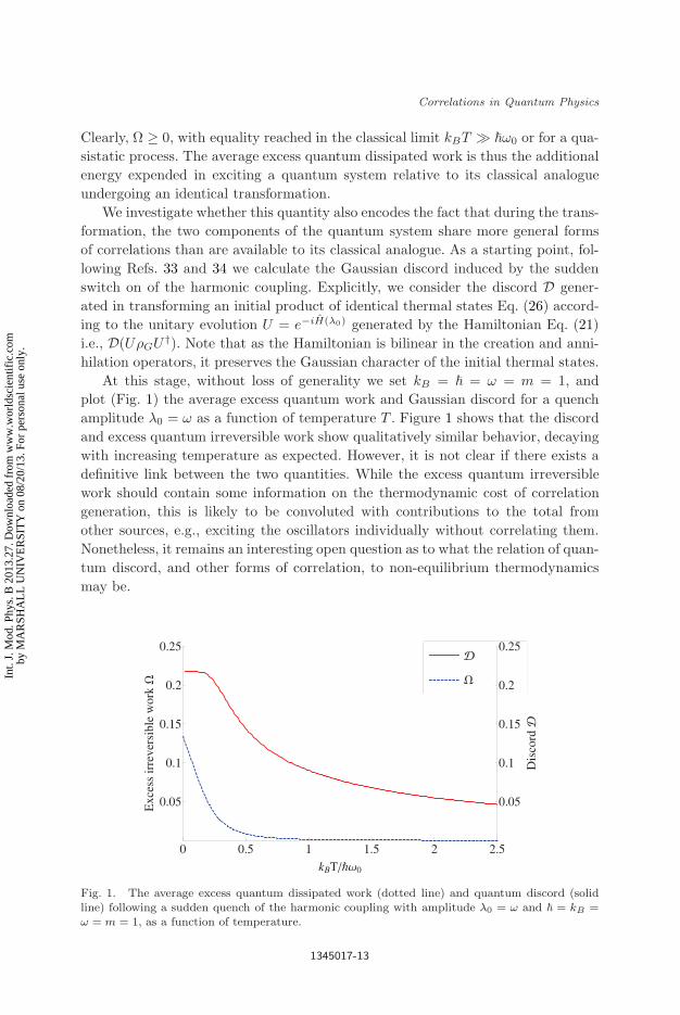
At this stage, without loss of generality we set kB = ~ = ω = m = 1, and

plot (Fig. 1) the average excess quantum work and Gaussian discord for a quench

amplitude λ0 = ω as a function of temperature T . Figure 1 shows that the discord

and excess quantum irreversible work show qualitatively similar behavior, decaying

with increasing temperature as expected. However, it is not clear if there exists a

definitive link between the two quantities. While the excess quantum irreversible

work should contain some information on the thermodynamic cost of correlation

generation, this is likely to be convoluted with contributions to the total from

other sources, e.g., exciting the oscillators individually without correlating them.

Nonetheless, it remains an interesting open question as to what the relation of quan-

tum discord, and other forms of correlation, to non-equilibrium thermodynamics

may be.

W

D

0 0.5 1 1.5 2 2.5

0.05

0.1

0.15

0.2

0.25

0.05

0.1

0.15

0.2

0.25

kBTÑΩ0

Excessirre

vers

ible

workW

Dis

cord

D

Fig. 1. The average excess quantum dissipated work (dotted line) and quantum discord (solidline) following a sudden quench of the harmonic coupling with amplitude λ0 = ω and ~ = kB =ω = m = 1, as a function of temperature.

1345017-13

Int.

J. M

od. P

hys.

B 2

013.

27. D

ownl

oade

d fr

om w

ww

.wor

ldsc

ient

ific

.com

by M

AR

SHA

LL

UN

IVE

RSI

TY

on

08/2

0/13

. For

per

sona

l use

onl

y.



Acknowledgments

The authors thank John Goold, Janet Anders, Kavan Modi, Myungshik Kim and

Marco Genoni for interesting and helpful discussions relating to the topic of this

work. RD is funded by the EPSRC. VV is a fellow of Wolfson College Oxford.

The authors acknowledge financial support from the Templeton Foundation, the

Leverhulme Trust, the National Research Foundation and the Ministry of Education

in Singapore.

References

1. C. Shannon, Bell Syst. Tech. J. 27, 379 (1948).2. H. Everett, On the foundations of quantum mechanics, Ph.D. thesis, Princeton Uni-

versity, Department of Physics (1957).3. O. Penrose, Rep. Prog. Phys. 42, 1937 (1979).4. G. Lindblad, Nonequilibrium Entropy and Irreversibility (Springer, Heidelburg, 1983).5. A. M. Kolmogorov, Foundations of the Theory of Probability (Chelsea, New York,

1950).6. J. von Neumann, Mathematical Foundations of Quantum Mechanics (Princeton Uni-

versity Press, New Jersey, 1955).7. G. W. Mackey, Mathematical Foundations of Quantum Mechanics (W. A. Benjamin,

New York, 1963).8. A. S. Holevo, Probabilistic and Statistical Aspects of Quantum Theory (North-Holland,

New York, 1982).9. M. Ohya and D. Petz, Quantum Entropy and Its Use (Springer-Verlag, Berlin, 1993).

10. R. S. Ingarden, A. Kossakowski and M. Ohya, Information Dynamics and Open Sys-

tems (Kluwer, Berlin, 1997).11. A. Wehrl, Rev. Mod. Phys. 50, 2 (1978).12. V. Vedral, Rev. Mod. Phys. 74, 197 (2002).13. H. Umegaki, Kodai Math. Sem. Rep. 14, 2 (1962).14. H. Araki and E. H. Lieb, Commun. Math. Phys. 18, 2 (1970).15. E. T. Jaynes and F. W. Cummings, Proc. IEEE. 51, 1 (1963).16. R. F. Werner, Lett. Math. Phys. 17, 359 (1989).17. R. F. Werner, Phys. Rev. A 40, 4277 (1989).18. R. Horodecki et al., Rev. Mod. Phys. 81, 865 (2009).19. E. Schrodinger, Naturwiss 23, 807 (1935).20. V. Vedral et al., Phys. Rev. Lett. 78, 2275 (1997).21. S. Popescu, Phys. Rev. Lett. 74, 2619 (1995).22. C. H. Bennett et al., Phys. Rev. Lett. 76, 722 (1996).23. V. Vedral and M. B. Plenio, Phys. Rev. A 57, 1619 (1998).24. L. Amico et al., Rev. Mod. Phys. 80, 1 (2008).25. J. Lee et al., J. Mod. Opt. 47, 12 (2000).26. J. Eisert and M. B. Plenio, Int. J. Quant. Inf. 1, 479 (2003).27. K. Modi et al., Phys. Rev. Lett. 104, 080501 (2010).28. L. Henderson and V. Vedral, J. Phys. A: Math. Gen. 34, 6899 (2001).29. V. Vedral, Phys. Rev. Lett. 90, 050401 (2003).30. L. Henderson and V. Vedral, Phys. Rev. Lett. 84, 2263 (2000).31. H. Ollivier and W. H. Zurek, Phys. Rev. Lett. 88, 017901 (2001).32. W. H. Zurek, Annalen der Physik (Leipzig) 9, 853 (2000).33. G. Adesso and A. Datta, Phys. Rev. Lett. 105, 030501 (2010).

1345017-14

Int.

J. M

od. P

hys.

B 2

013.

27. D

ownl

oade

d fr

om w

ww

.wor

ldsc

ient

ific

.com

by M

AR

SHA

LL

UN

IVE

RSI

TY

on

08/2

0/13

. For

per

sona

l use

onl

y.



34. P. Giorda and M. G. A. Paris, Phys. Rev. Lett. 105, 020503 (2010).35. F. Galve and E. Lutz, Phys. Rev. A 79, 032327 (2009).36. F. Galve, Phys. Rev. A 84, 012318 (2011).37. M. B. Plenio, J. Hartley and J. Eisert, New J. Phys. 6, 36 (2004).38. J. Eisert et al., Phys. Rev. Lett. 93, 190402 (2004).39. J. D. Walecka, Fundamentals of Statistical Mechanics: Manuscript and Notes of Felix

Bloch (Imperial College Press, UK, 2000).40. V. Sudhir et al., Phys. Rev. A 86, 012316 (2012).41. P. Talkner, E. Lutz and P. Hanggi, Phys. Rev. E 75, 5 (2007).

1345017-15

Int.

J. M

od. P

hys.

B 2

013.

27. D

ownl

oade

d fr

om w

ww

.wor

ldsc

ient

ific

.com

by M

AR

SHA

LL

UN

IVE

RSI

TY

on

08/2

0/13

. For

per

sona

l use

onl

y.

correlations in quantum physics

Documents