7.3

Correlation-Preserved Analysis with

Non-Gaussian Statistical Timing Quadratic Timing Model

Lizheng Zhang, Weijen Chen, Yuhen Hu, John A. Gubner, Charlie Chung-Ping Chen

{lizhengz,weijen} 8 cae.wisc.edu,{hu,gubner,chen} @ engr.wisc.edu ECE Department,University of Wisconsin, Madison, W153706-1691, USA

ABSTRACT Recent study shows that the existing first order canonical timing model is not sufficient to represent the dependency of the gate delay on the variation sources when processing and operational variations become more and more signifi- cant. Due to the nonlinearity of the mapping from variation sources to the gate/wire delay, the distribution of the de- lay is no longer Gaussian even if the variation sources are normalIy distributed.

A novel quadratic timing model is proposed to capture the nonlinearity of the dependency of gate/wire delays and arrival times on the variation sources. Systematic method- ology is also developed to evaluate the correlation and dis- tribution of the quadratic timing model. Based on these, a. novel statistical timing analysis algorithm is propose which retains the complete correlation information during timing analysis and has the same computation complexity as the algorithm based on the canonica1 timing model.

Tested 011 the ISCAS circuits, the proposed algorithm shows IOx accuracy improvement over thc existing first or- der algorithm while no significant extra runtime is needed.

Categories and Subject Descriptors B7.2 Hardware [INTEGRATED CIRCUITS]: Design Aids- Verification

Genera1 Terms Algorithms, Performance, Verification

1. INTRODUCTION The timing performance of deep-submicron micro-architecture

will be dominated by several factors. IC manufacturing p r e cess parameter variations will cause device and circuit pa- rameters to deviate from their designed value. Low supply voltagc for low-power applications will reduce noise margin, causing increased timing delay variations. Due to dense inte- gration and non-ideal on-chip power dissipation, rising tem-

Permission to make digital or hard copies of all or part of this work for personal or classroom use is granted without fee provided that copies are not made or distributed for profit or commercial advantage and that copies bear this notice and the full citation on the first page. To copy otherwise, to republish, to post on servers or to redistribute to lists, requires prior specific permission and/or a fee. DAC2005, June 13-1 7,2005, Anaheim, Califomia. USA.

perature of substrate may lead to hot spot, causing excessive timing variations. Classical worst case timing analysis pro- duces timing predictions that are often too pessimistic and grossly conservative. On the other hand, statistical timing analysis (STA) that characterizes timing delays as statistical random variables offers a better approach for more accurate and realistic timing prediction.

Existing STA methods can be categorized into two dis- tinct approaches: path based STA [l-41 and block based STA 15-111. The path based approach seeks to estimate timing statistically on selected critical paths. However, the task of selecting a subset of paths whose time constraints are statistically critical has a worst-case complexity that grows exponentially with respect to the circuit size. Hence it is not easily scalable to handle realistic circuits. The block based approach, on the other hand, champions the notion of pro- gressive computation. Specifically, each gate/wire is treated as a timing block and the timing analysis i s performed block by block in the forward direction in the circuit timing graph without looking back to the path history. As such, the com- putation complexity would grow linearly with respect to the circuit size.

However, to realize the fuIl benefit of block based STA, one must address a challenging issue that gate/wire delays in a circuit could be correlated since two delays might be affected by the same variation sources of global variations such as voltage supply uncertainties, gate channel length variations, wire geometry variations, ..., etc. In [6,7,10] the delay D is explicitly related with these global variations G, by the canonzml timing model

where R, called local variation, accounts the cumulative ef- fect of variation sources other than considered global varia- tions.

The canonical timing model (1) provides an elegant way to deal with the correlations( [lo]). Unfortunately, the nonlin- ear relationship between the gate/wire delay and the global variation sources can not be accurately approximated by the current linear canonical timing model. And even the global variations are often modeled as Gaussian random variables( [12,13]) , the gate/wire delays, in general, will not be Gaussian distributed random variables. This yields un- satisfactory results for deep-sub-micron IC circuit where rel- ative magnitudes of global variations are often larger, while more accurate STA is demanded.

To mitigate this deficiency, in this paper, we propose - - - - Copytight 2005 ACM 1-59593-058-2/05/oOo6 ... $5.00. a novel quadratic timing model that augments the linear

83

canonical timing model with second order terms:

D = m + CYR + PIG, + I’ijGiGj (2) i i , j

where Ti, are quadratic coefficients and m is a constant term which may be different from the mean value of the delay timing variable.

timing model delivered 4x accuracy improvement over a first order canonical model. Nevertheless, [ 141 does not address the important question of how to systematically develop a quadratic timing model to p e r f o m accurate STA of large scale circuits. The main objective of this paper is to de- velop such a practical, efficient solution to this question. To this aim, we have made a number of tangible contributions:

(1) A novel quadratic timing model is formulated for both gate/wire delay and signal arrival time to represent the cor- relation between them. Systematic methodology is also de- veloped to evaluate the correlations and to compute distri- butions for the quadratic timing model.

(2) A novel statistical timing algorithm is developed based on the quadratic timing niodel which successfully retains the complete correlation information among arrival times during timing analysis while has the same computation complexity as algorithms based on canonical timing model.

(3) A novel conditional linear M A X approximation method is proposed to deal with cases when MAX operator is signif- icantly non-linear. By assuming inputs to be Gaussian, we are able to detect the linearity of the MAX operator by just checking the skewness of the output. Linear approximation of MAX is only used when MAX is decided to be linear. If MAX is non-linear, the evaluation is delayed within a for- mat of M A X tuple until it becomes h e a r in the later timing steps.

The rest of the paper is organized as following: Section 2 presents the quadratic timing model for gate/wire delay and the arrival time; Section 3 introduces the mathemat- ics tools used for correlation and distribution evaluation for quadratic timing model; Section 4 describes the statistical timing algorithm based on the quadratic timing model; Sec- tion 5 presents the C/C++ implementation and tcsting re- sults; Section 6 gives the conclusions.

Preliminary work reported in [14] indicated that a quadratic

2. QUADRATIC MODEL OF TIMING VARI-

Since the time variables, either gate/wire delays or arrival times, are modeled as non-Gaussian random variables, the mean(p) and std(a), uscd for canonical delay cases, are not sufficient to characterize the distributions of the time ran- dom variables. For the interest of the timing analysis, we define a third parameter to assist the distribution charac- terization:

Definition 1. FOT a random time variable X , i t s equiv- alent two sigma value, abbreviated as ‘k2u”, is defined as:

P ( X < e%) = 97.7%

Except the special case of Gaussian random variable, e 2 ~ # p + 2u in general. Knowing this, we hereafter pay more attention to e 2 0 than the mean and std since it is e2u that really means performance of the considered circuit.

2.1 Quadratic Gate Delay Model It is generally accepted that the gate delay D, is a nonlin-

ear function of the global variation variables. We formulate the quadratic gate delay model by taking the second order Taylor expansion of D, with respect to the global variation variables (evaluated around the mean value of these global variations) :

D, E m , + r u ~ + ~ ~ + ~ I / + ... l3L L3V

In this equation, mg is a constant and L, V... are gIobal variations. The coefficients in this Taylor expansion can be andytically extracted from the Spice model of the gate delay. Hence, in the following discussion, we will assume these parameters are known in advance.

Assume that there are p global variation variables, one may define a p x 1 Gaussian variation vector

where “*” represents the transpose operation. 0 is a zero vector. The cowelation matrix (Eg = E{6,6;]) is a p x p matrix. Generally it is not a unit matrix I since these global variation random variables may be correlated among themselves.

Consolidate equations (2) and (3) into a compact quadratic form:

D, = m, + aR + P:S, + Sif,S, (4)

where the vector p, and matrix rs are only vectorized r ep resentation of the Taylor expansion coefficients in equation

.’/

(a) c.d.f. of Inverter Delay (b) p .d . f . of Inverter Delay

Figure 1: Distributions of Inverter Delay

To demonstrate the advantage of the quadratic gate de- lay model over the first order canonical model, the probabil- ity distribution of an inverter delay is estimated using the Monte Carlo method where the timing delay of each trial is evaluated using SPICE circuit simulator. Using the param- eters analytically extracted from the SPICE model, the de- lay distributions are also computed using both the quadratic timing model and the linear canonical timing model. Shown in figure l(b), the “true” distribution from Monte Carlo sim- ulation is significantly non-symmetric and non-Gaussian and can not be approximated by any canonical timing model.

84

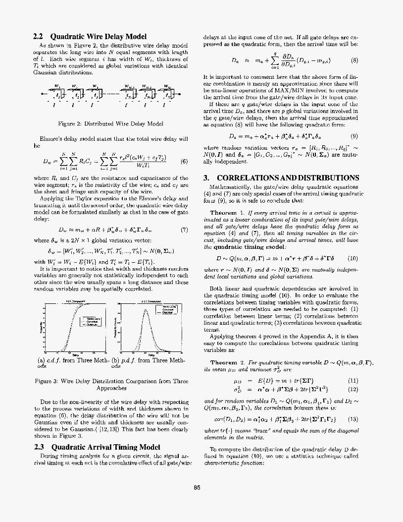
2.2 Quadratic Wire Delay Model As shown in Figure 2, the distributive wire delay model

separates the long wire into N equal segments with length of 1. Each wire segment i has width of Wi, thickness of T, which are considered as global variations with identical Gaussian distributions.

1 I I

Figure 2: Distributed Wire Delay Model

Elmore's delay model states that the total wire delay will be

where Ri and Cj are the resistance and capacitance of the wire segment; T, is the resistivity of the wire; cg and cf are the sheet and fringe unit capacity of the wire.

Applying the Taylor expansion to the Elmore's delay and truncating it until the second order, the quadratic wire delay model can be formulated similarly as that in the cme of gate delay:

where 6 , is a 2N x 1 global variation vector:

with W,! = Wi - E{Wi} and T,! = Ti - E(T,}. It is important to notice that width and thickness random

variables are generally not statistically independent to each other since the wire usually spans a long distance and these random variables may be spatially correlated.

P" ! :I- :[ j ,I 1

. m m - s - w (a) c.d.f . from Three Meth- ods

Figure 3: Wire Delay Distribution Comparison from Three Approaches

Due to the non-linearity of the wire delay with respecting to the process variations of width and thickness shown in equation (6), the delay distribution of the wire will riot be Gaussian even if the width and thickness are usually con- sidered to be Gaussian.( [12,13]) This fact has been clearly shown in Figure 3.

2.3 Quadratic Arrival Timing Model During timing analysis for a given circuit, the signal ar-

rival timing at each net is the cumulative effect of all gate/wire

delays at the input cone of the net. If all gate delays are ex- pressed as the quadratic form, then the arrival time will be:

It is important to comment here that the above form of lin- ear combination is merely an approximation since there will be non-linear operations of MAX/R/IIN involved to compute the arrival time from the gate/wire delays in i t s input cone.

If there are q gate/wire delays in the input cone of the arrival time D,, and there are p global variations involved in the q gate/wire delays, then the arrival time approximated as equation (8) will have the following quadratic form:

D, ma + a : ~ a + p;s, -t s:r,s, (9)

where random variation vectors ra = [ R I , Rz, ..., Rs]* N

N ( 0 , I ) and 6 a = [G1,G2,. . . ,GP]* N N ( O , C , ) are mutu- ally independent.

3. CORWLATIONS AND DISTIUBUTIONS Mathematically, the gate/wire delay quadratic equations

(4) and (7) are only special cases of the arrival timing quadratic form (9), so it is safe to conclude that:

Theorem 1. I f every arrival t ime in a circuit is appmx- imated as a linear combination of its input gate/wire delays, and all gate/wire delays have the quadratic delay f o r m as equation (4) and (7), then all timing variables in the cir- cuit, including gate/wire delays and arrival times, will have the quadratic timing model:

D - Q(m,a,p, r) = m + a * ~ + /3*S + &*I?& (10)

where T - N ( 0 , I ) and 6 -+ N ( 0 , X) are mutually indepen- dent local variations and global variations.

Both linear and quadratic dependencies are involved in the quadratic timing model (10). In order to evaluate the correlations between timing variables with quadratic forms, three types of correlation are needed to be computed: (I) correlation between linear terms; (2) correlations between linear and quadratic terms; (3) correlations between quadratic terms.

Applying theorem 4 proved in the Appendix A, it is then easy to compute the correlations between quadratic timing variables as:

Theorem 2. For quadratic timing variable D - &(mi a, p, r), its mean D D and variance & are

p D = ~ { ~ ) = m + t r { ~ r ) (11) = a*a + p * ~ p 3- z t T p 2 r 2 } (12)

and for random variables DI - Q ( T T L ~ , ~ I , & , ~ I ) and D2 - Q(m2, az, p2, Fz), the correlation between them is:

where t r ( . } means "trace" and equals the sum of the diagonal elements in the matrix.

To compute the distribution of the quadratic delay D de- fined in equation (lo), we use a statistics technique called characteristic function:

85

Theorem 3. If the mndom variable X has a chamcteris- t i c function of Cx(<), then the p.d. f . of the random variable X will be:

The formal proof of this theorem can be found in textbooks of probabilistic theory such as 1151.

For the quadratic timing variable D N Q(m, &,PI I?) de- fined in equation (lo), its exact characteristic function can be analytically derived as:

1 1 where is the determinant of matrix n = 1 - 2 j < E ~ r E ~ . So the p.d.f. of the quadratic time variable, f~(z), can then be computed from theorem 3.

4. STA WITH QUADRATIC TIMING MODEL In block based STA, the arrival time random variable

propagation involves two elemental operations: (1)ADD: When an input arrival time X propagates through

a gate delay Y , the output arrival time will be 2 = X + Y ; ( 2 ) M A X : When two arrival times X and Y merge in a

gate, a new arrival time of Z = m a x ( X , Y ) will be formu- lated before the gate delay is added.

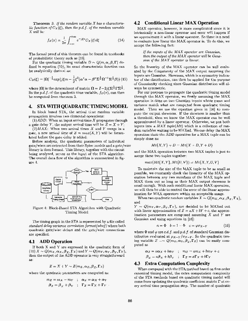
Before analysis, the quadratic parameters of individual gatelwires are extracted from their Spice models and a gate/wire library is then formed. This library, together with the circuit being analyzed, serves as the input of the STA algorithm. The overall data flow of the algorithm is summarized in fig- ure 4.

Figure 4: Block-Based STA Algorithm with Quadratic Timing Model

The timing graph in the STA is represented by a file called standard delay variance correlation format(sdvcf) where both quadratic gatelwire delays and the gate/wire connections are specified.

4.1 ADD Operation If both X and Y are expressed in the quadratic form of

(1O)X N Q(mx,ax,Px,rx)andYNQ(mY,(Xy,P=,rY), then the output of the ADD operator is very straightforward as:

z = x + Y z(mz,az,pz,rz) where the quadratic parameters are computed as:

m z = m x + m u ; a z = a x + f f u p z = p x + p y ; r z = r x + r y

4.2 Conditional Linear MAX Operation MAX operator, however, is more complicated since it is

intrinsically a non-linear operator and error will happen if we approximate it with a linear operator. So there is a need to evaluate how linear the MAX operator is. TO do this, we accept the following fact:

If the inputs of the M A X operator are Gaussim, then the output of the MAX operator wall be Gaus- sian i f the M A X operator is linear.

So the linearity of the MAX operator can be well evalu- ated by the Gaussianity of the MAX output assuming the inputs are Gaussian. Skewness, which is a symmetry indica- tor of the distribution, can then be applied for the purpose of Gaussianity checking since Gaussian distribution will al- ways be symmetric.

For our purpose to propagate the quadratic timing model through the MAX operator, we firstly assuming the MAX operation is done on two Gaussian inputs whose mean and variance match what are computed from quadratic timing model. Then we use the equation given in [16] to com- pute the output skewness. If the skewness is smaller than a threshold, then we know the MAX operator can be well approximated by a linear operator. Otherwise, we put both inputs into a M A X tuple(Mt) which is a collection of ran- dom variables waiting to be MAXed. We can delay the MAX operation since the ADD operation for a MAX tuple can be simply done as:

M t { X , Y ) + D = M t { X + D , Y + D }

and the MAX operation between two MAX tuples is just to merge these two tuples together:

m a z ( M t { X , Y } , Mt{U, V)) = M t { X , Y, U, V}

To maintain the size of the MAX tuple to be as small as possible, we constantly check the linearity of the MAX o p eration between any two members of the MAX tuple and MAX them out as long as their MAX output skewness is small enough. With such conditional linear MAX operation, we will then be able to control the error of the linear approx- imation for MAX operators within an acceptable range.

and Y - Q ( ~ Y , Q Y , ~ ~ , ~ Y ) , are decided to be MAXed out with linear approximation of 2 = aX + bY + c, the approx- imation parameters are computed assuming X and Y are Gaussian and using equations in [16]:

When two quadratic random variables X N &(mx, OX, Px, rx),

a = @ b = 1 - @ c = ( p u x - y (16) where 9 and 'p are c.d.f. and p.d.f. of standard Gaussian dis- tribution evaluated at p x - y l u x - y . So the quadratic tim- ing variable Z =- Q(mz,az,pz,rz) can be easily corn- puted a s

az = a a x + b a y ; mz = amx + b m y + c P z = a @ , + b P y ; r z = a r X + b r y

4.3 Extra Computation Complexity When compared with the STA method based on first order

canonical timing model, the extra computation complexity of the STA methods based on quadratic timing model will come from updating the quadratic coefficient matrix l? at ev- ery arrival time propagation step. The number of quadratic

86

Table 1: Distribution Parameters for ISCAS Circuits with three Approaches: (1)Monte Carlo(M.C.); (2)Canonical Model(CanoStat); (3)Quadratic Model(QuaclStat)

coefficients is limited by the number of considered global variations and is usually a constant. Updating matrix r will not, increase the computation complexity since it only involves moment computation of quadratic timing variables whichis not dependent on the circuit size.

So briefly, the computation complexity of STA based on quadratic timing model will be the same as its canonical timing niodel correspondence.

4.4 Application in Path Based STA Although we propose above a block based STA method

because path based STA will have potential difficulty to se- lect statistically critical paths in complex circuits, nothing prevents us applying the proposed quadratic timing model in path based STA.

As long as the statistically critical paths are correctly s e lected, the overall delay distribution of the circuit can be computed very straightforwardly. For the i th critical path cpi, its path delay will be Dcyi = CgEcpi D,. When all gate/wire delays are quadratically represented, the path d e lay will also have quadratic format as:

N Q( mg, a g : P,, r,) (17) $€CPi O E C P Z gEcpi g E c p i

So if there are R statistically critical paths, the overall delay distribution will be:

Dall = "(&l, D c p a , ..., Dcpn) (18)

where the MAX operation is token in the statistical sense.

5. SIMULATIONS AND DISCUSSIONS The proposed block based STA with quadratic timing

model has been implemented in C/C++ with the name of Quadstat and tested on the ISCAS'85 benchmark circuits. For comparison, we also implement the STA bayed on first order canonical timing model, named CunoStat, is also im- plemented and tested. Monte Carlo simulation with 10,000 repetitions is used as a comparison standard.

All ISACS circuits are re-mapped into a simple standard gate library with gates of not, nand$ nand3, LOT^, "3, zor,/mor. All these standard gates are implemented with Cadence took. Their quadratic timing model parameters arc extracted from their Spice model with the variations specified by the technology file.

5.1 Accuracy Improvement Timing results from both Quadstat and CunaStat are

shown in Table 1 and compared with that from Monte Carlo simulation.

The estimation error is also shown in the table from which it is clear that there is a significant accuracy improvement just by switching the delay model from canonical t o quadratic. Measured by the performance critical parameter of equiva- lent two sigma delay of the circuit, e2a, average lox accu- racy improvement is achieved: the average error of CanoStat is 24% while that of QuadStat is small as 2.3%.

. .

7p; , ,",\ I .I J , , , , , , , 1 " .

-ia&i= - - - '-

(b) c d f . of ISCAS c3540 Figure 5: Distribution Comparison of ISCAS c3540 from Three Approaches: (1)Monte Carlo; (2)Canonical Model;

(3)Quadratic Model

'r . m m m m w " w - # - *o U - -

w d . Y lprl

(a) p.d.f. of ISCAS c3540

To graphically illustrate the accuracy improvement, the delay distributions of ISCAS circuit c3540 are show in figure 5. It is clear that the accuracy improvement of the QuadStat is mostly due to the high probability region of the distribu- tion which is actually more critical for circuit performance. CanoStat will clearly underestimate the delay in the high probability region. This underestimation, in reality, will rc+ sult in optimistic design and excessive chip failure. This ex- ample clearly shows the necessary to use quadratic timing model when variations becomc large in nowadays technol- om. 5.2 Performance Comparison

The CPU time of the three approaches is shown in Table 2 where it is clear that tremendous time is save from Monte Carlo simulation by using either QuadStat and CanoStat. And also, it is clear that there is no significant running time difference between QuadStat and CanoStat which demon- strates the conclusion we made in section 4.3: NO extra computation is needed to switch fmm canonical STA meth- od$ to quadratic STA methods.

87

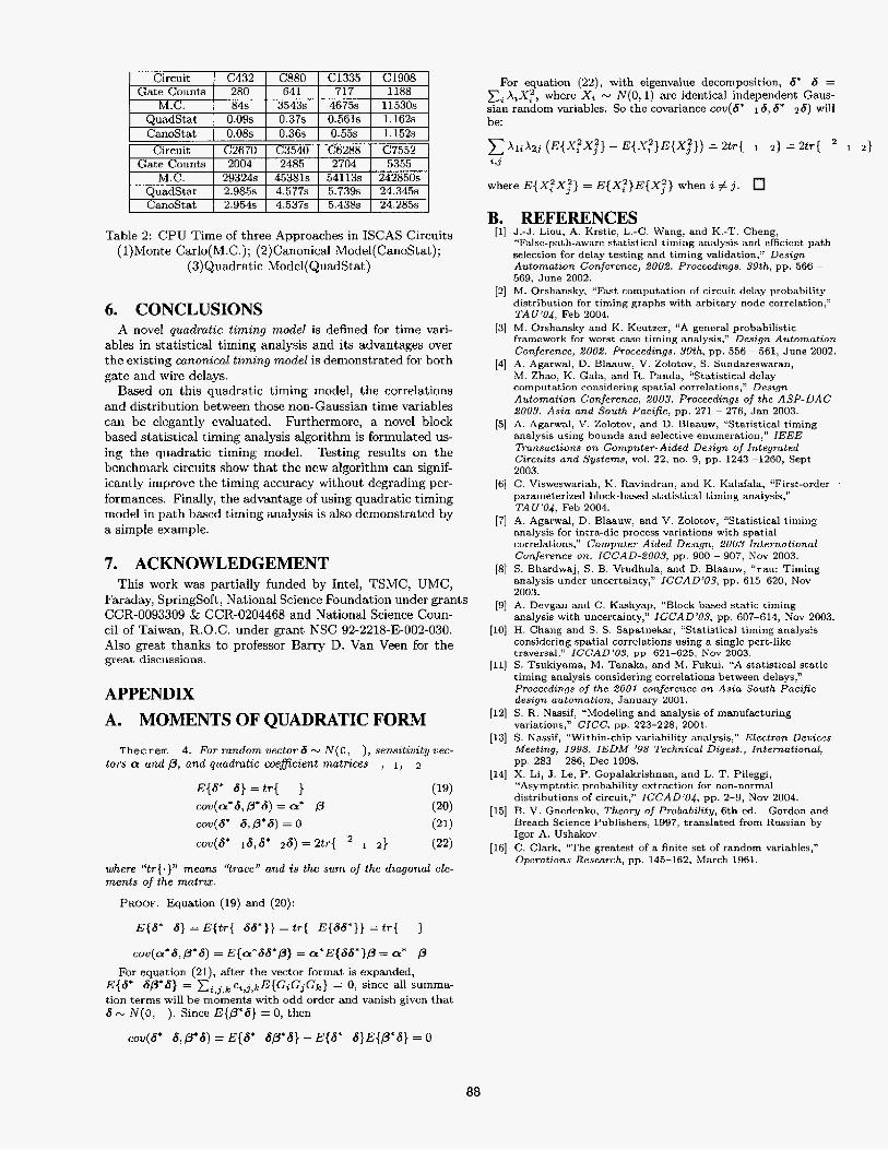
Circuit

M.C. 3543s 4675s 11530s QuadStat 0.09s 0.37s 0.561s 1.162s CanoStat 0.08s 0.36s 0.55s 1.152s Circuit C2670 C3540 C6288 C7552

M.C. 29324s 45381s 54113s 242850s QuadStat 2.985s 4.577s 5.739s 24.345s CanoStat 2.954s 4.537s 5.438s 24.285s

Table 2: CPU Time of three Approaches in ISCAS Circuits (1)Monte Carlo(M.C.); (2)Canonical Model(CanoStat);

(3)Quadratic Model(QuadStat)

6. CONCLUSIONS A novel quadmtic timing model is defined for time vari-

ables in statistical timing analysis and its advantages over the existing canonical timing model is demonstrated for both gate and wire delays.

Based on this quadratic timing model, the correlations and distribution between those non-Gaussian time variables can be elegantly evaluated. Furthermore, a novel block based statistical timing analysis algorithm is formulated us- ing the quadratic timing model. Testing results on the benchmark circuits show that the new algorithm can signif- icantly improve the timing accuracy without degrading per- formances. Finally, the advantage of using quadratic timing model in path based timing analysis is also demonstrated by a simpte example.

7. ACKNOWLEDGEMENT This work was partially funded by Intel, TSMC, UMC,

Faraday, Springsoft, National Science Foundation under grants CCR-0093309 & CCR-0204468 and National Science Coun- cil of Taiwan, R.O.C. under grant NSC 92-2218-E002-030. Also great thanks to professor Barry D. Van Veen for the great discussions.

APPENDIX A. MOMENTS OF QUADRATIC FORM

Theorem 4. For madom vector6 N N ( 0 , ), semztavrty vec- tors a and /3, and quadratzc coeficzent matnces , I , 2

E{S* 6) = t r { } (19) cou(ck*B,p*9) = a* p (20) cOv(a* 8,0*6) = 0 (21)

(22) cov(6* 16,6* 2 9 ) = 2tr{ 2 1 2)

where “tr{.}’’ means “tmce” and is the sum of the dzagonal ele- ments of the matrix.

PROOF. Equation (19) and (20):

E{6* 6) = E(tT{ 66’1) = tr{ E { S 6 * } ) = tr{ 3 c o v ( a * d , P ’ 6 ) = E{a*dd*/3} = a*E{66*)P = a*

For equation (Zl), after the vector format is expanded, P

E{&* S@*S} = Cr,j,A: C , , ~ , ~ E { G , G , G ~ } = 0, since all summa- tion terms will be moments with odd order and vanish given that 6 N N ( 0 . ). Since E { V S } = 0, then

COW(&* S,/3*6) = E{&* SP’S} -E{&* 6 } E { / 3 * 6 ) = 0

For equation (22), with eigenvalue decomposition, 6* 6 = E, X,Xp, where X, N N ( 0 , l ) are identical independent Gaus- sian random variables. So the covariance m ( 6 * IS,&* 2 6 ) will be:

x1~x23 ( E { X , ~ X , ~ } - E { x , ~ ) E { x , ~ ) ) = 2 t ~ { 2 ) = 2 t ~ { d. 1.3

where E{X:X:) = E(X~}E{X~} when z # 3,

REFERENCES J.4. Lou, A. Krstic, L.-C. Wang, and K.-T. Cheng, “False-path-aware statistical timing analysis and efficient path selection for delay testing and timing validation,” Design Automation Conference, 2002. Proceedings. Sgth, pp. 566 ~

569, June 2002. M. Orshansky, “Fast computation of circuit delay probability distribution for timing graphs with arbitary node correlation,” TA U’O4, Feb 2004. M . Orshansky and K. Keutzer, “A general probabilistic framework for worst case timing analysis,” Design Automation Conference, 200%. Proceedings. 39th, pp. 556 ~ 561, June 2002. A. Agarwal, D. Blaauw, V. Zolotov, S. Sundareswaran, M . Zhao, K. Gaia, and R. Panda, “Statistical delay computation considering spatial correlations,” Design Automation Conference, 2003. Proceedings of the ASP-DAC 2009. Asia a n d South Paczfk: pp. 271 - 276, Jan 2003. A. Agarwal, V. Zolotov, and D. Blaauw, “Statistical timing analysis using bounds and selective enumeration,” IEEE Transactions o n Computer- Aided Design of Integrated Corcurts and Systems, vol. 22, no. 9, pp. 1243 -1260, Sept 2003. C. Visweswariah, K. Ravindran, and K. Kalafala, “First-order parameterized block-based statistical timing anaiysis,” TA U’U& Feb 2004. A. Agarwal, D. Blaauw, and V. Zolotov, “Statistical timing analysis for intra-die process variations with spatial correlations,” Computer A i d e d Design, 2003 International Conference on. ICCAD-2003, pp. 900 - 907, Nov 2003. S. Bhardwaj, S. B. Vrudhula, and D. Blaauw, “Tau: Timing analysis under uncertainty,” ICCAD ’09, pp. 615-620, Nov 2003. A. Devgan and C. Kashyap, “Block-basad static timing analysis with uncertainty,” I C C A D ‘03, pp. 607-614, Nov 2003. H. Chang and S. S. Sapatnekar, L‘Statistical timing analysis considering spatial correlations using a single pert-like traversal,” ICCAD’OS, pp. 621-625, Nov 2003. S. Tsukiyama, M. Tanaka, and M. Fukui, “A statistical static timing analysis considering correlations between delays,” Proceedings of the 2001 conference on Asia South Pacific design automation, January 2001. S. R. Nassif, “Modeling and analysis of manufacturing variations,” CICC, pp. 223-228, 2001. S. Nassif, “Within-chip variability analysis,” Electmn Devices Meeting, 1998. IEDM ’98 Technical Digest., International, pp. 283 ~ 286, Dec 1998. X. Li, J. Le, P. Gopalakrishnan, and L. T. Pileggi, “Asymptotic probability extraction for non-normal distributions of circuit,” ICCAD’U4, pp, 2-9, Nov 2004. B. V. Gnedenko, Theory 01 Probability, 6th ed. Breach Science Publishers, 1997, translated from Russian by Igor A. Ushakov. C. Clark, “The greatest of a finite set of random variables,” Operations Research, pp. 145-162, March 1961.

Gordon and

88