correlation of pressure drop for two-phase, a thesis …
TRANSCRIPT

CORRELATION OF PRESSURE DROP FOR TWO-PHASE,
CONCURRENT FLOW IN PACKED BEDS
by
HANG-YEN FANG, B.S. IN CH.E.
A THESIS
IN
CHEMICAL ENGINEERING
Submitted to the Graduate Faculty of Texas Tech University in
Partial Fulfillment of the Requirements for
the Degree of
MASTER OF SCIENCE IN
CHEMICAL ENGINEERING
Approved
Accepted
December, 1981

ACKNOWLEDGMENTS
The author wishes to express his great appreciation
to the following people for their contributions to the
research which was the basis of this thesis:
Dr. L. D. Clements, Jr., chairman of the committee,
for his wise counsel, for his interest and enthusiasm, and
for his cooperation on every occasion.
Drs. S. R. Beck and S. Selim, committee members, for
their assistance and suggestions during the progress of
this work.
Mr. C. Y. Lee for his successful preparation.
My wife, Pi-Fei, first for her patient typing work,
but most of all, for her understanding and encouragement
during the course of this work.
ii
.- .. ··

TABLE OF CONTENTS
ACKNOitJLEDGMENT S . . . . . . . . . . . . . . . . . . . . . . . . . . . . . . . . . . . . . I I I I I I I I I I I I I I I I I I I I I I I I I I I I I I I I I I I I I
. . . . . . . . . . . . . . . . . . . . . . . . . . . . . . . . . . . . . LIST OF TABLES
LIST OF FIGURES
NOMENCLATURE I I I I I I I I I I I I I I I I I I I I I I I I I I I I I I I I I I I I I I I
CHAPTER I INTRODUCTION ..... o o o o o o o o o o o •• o o o • o • o • o •
Objectives . . . . . . . . . . . . . . . . . . . . . . . . . . . . CHAPTER II LITERATURE REVIEW
Liquid Holdup I I I I I I I I I I I I I I I I I I I I I I I I I
Pressure Drop in Single Phase Flow
page
ii
iv
v
Vll
l
5
6
7
in Packed Beds o • 0 ••• o • 0 o 0 0 o o 0 o o 0 o o 0 o • • 10
Two Phase Flow Pressure Drop a o • • • • • • 1 •
CHAPTER III THEORETICAL ANALYSIS I I I I I I I I I I I I I I I I I I
Energy Balance . . . . . . . . . . . . . . . . . . . . . . . ..__,
Model 0 I I I I I I I I I I I I I I I I I I I I I I I I I I I I I I I I
CHAPTER IV CORRELATION AND DISCUSSIONS
Data Characteristic . . . . . . . . . . . . . . . . . . . Correlation of Experimental Data
Result of Correlation a • • • • • • • • • • • • • • • •
Discussions . . . . . . . . . . . . . . . . . . . . . . . . . . . . CHAPTER V CONCLUSIONS AND SUGGESTIONS
Conclusions . . . . . . . . . . . . . . . . . . . . . . . . . . . Further Study Suggestions I I I I I I I I I I I I I
REFERENCES I I I I I I I I I I I I I I I I I I I I I I I I I I I I I I I I I I I I I I I I I
lll
18
39
39
41
52
52
56
67
70
81
81
81
83

LIST OF TABLES
page
Table I Comparison Between Countercurrent and Concurrent Operation II •• ~· Ill •••• II 2
Table II Holdup Correlations ~·· ....... I ••• I I •• I I 8
Table III Characteristics of Two-Phase Packed Bed Pressure Drop Data Used II .I ••••• Oil 53
Table IV Comparison of Correlations II. I ••• II •••• 71
iv

Figure
Figure
Figure
Figure
Figure
Figure
Figure
Figure
Figure
LIST OF FIGURES
page
1 Exponents for porosity function . . . . . . . . 12
2 Reynolds number vs. friction factor .... 13
3 fvvs. NRe/(1-E) ....................... 16
4 Comparison between Ergun's and Hick's equation . . . . . . . . . . . . . . . . . . . . . . . . . . . . . . . 17
5 Larkins' correlation ................... 23
6 Control surface for the momentum
7
8
9
exchange model of Turpin and Huntington . . . . . . . . . . . . . . . . . . . . . . . . . . . . . 26
The capillary model .................... 35
The capillary flow model I I I I I I I I a I I I I D I
The capillary saparation flow model .... 42
48
Figure 10 Log ( oLGE3DpReL Pu (L2 (1-E )2 )) vs.
Log(Rei/(1-E)) , GPuLPG in the range
Figure 11
Figure 12
Figure 13
170 to 200 ............................. 58
Log(oLGE3DpReL Pu(L2 (1-E) 2 ) vs.
Log(Rei/(1-E)), GPL/LPG in the range: 90 to 100 . . . . . . . . . . . . . . . . . . . . . . . . . . . . . . 59
Log(oLGE3DpReLPU(L2 (1-E) 2 ) vs.
Log(Rei/(1-E)), G PuL.PG in the range:
40 to 50 . . . . . . . . . . . . . . . . . . . . . . . . . . . . . . . 60
Log(oLGE3DpReLPU(L2 (1-E) 2 ) vs.
Log(Rei/(1-E)), G PUL PG in the range: 7 . 5 t 0 12 . 5 . . . . . . . . . . . . . . . . . . . . . . . . . . . . 61
v

Figure
Figure
Figure
Figure
Figure
Figure
Figure
14
15
16
17
18
19
20
Log(fTp/(Rei(l-E) 0 · 8 ) vs.
Spherical and cylindrical
Log(fTp/(Rei/l-E) 0•8 ) vs.
GPL Log (L p )
G packings
GPL Log (L p )
G
e I I I
page
63
Raschig ring packing .................. 64
fv vs. (G PL~G/LPG~L), @
Rei/ ( 1-E) less than 50 • • . . . . . . . . . . • . . • 66 @
Log((fTP-fv)/Fk) vs. Log(Rel/(1-E))
Spherical and cylindrical packings •... 68 @
Log((fTP-fv)/Fk) vs. Log(ReL/(1-E))
Raschig ring packing .................. 69
Distribution curve of error
Density distribution curves
vi
. . . . . . . . . . .
. . . . . . . . . . . 77
80

a v
Al'
Dp
D c
D e
* EuL
* EuG
fk
fv
fTP
G
* G
A2' A3
NOMENCLATURE
surface area per unit volume
coefficients of correlation groups
particle diameter
capillary diameter
equivalent diameter
- * 2 liquid Euler's number P atm'-L/(L )
gas Euler's number Patm ·~/(G*) 2
kinetic friction factor
viscous friction factor
friction factor for two phase flow 3 oLG .JL Dp ReL E
L2 (l-~)2
conversion factor, 32.17 poundals per pound
in English units
superficial gas flow rate in open column
(lb/ft 2 . hr)
average gas flowrate in packed bed (G/c)
liquid holdup
prediction holdup
true holdup
vii

1
* 1
n
F
F atm
* p
R
r c
s
t
u
dimensionless group * * * oF EuG.ReG
( ~ ) oZ 2
* * * oF Eu1 .Re1 ( ) *
dimensionless group oz 2
supercial liquid flow rate in open colu~n (lb/ft2 . hr)
average liquid flowrate in packed bed (1/E)
@ exponent of Re1/(l-E)
pressure
atmosphere pressure, 14.7 psi.
dimensionless group
radius
radius of capillary
F
Fatm
radius of the gas-liquid interface
DF G gas Reynolds number
gas Reynolds number at gas flowrate G/~
DF 1 liquid Reynolds number
u1
liquid Reynolds number at liquid flowrate 1/~
@ liquid Reynolds number at liquid velocity u
dimensionless interface radius, r 1/rc
the thickness of liquid along the wall of the
column
velocity viii

w
z
* z
Pm
E
velocity at the interface
velocity ( _b_ + p1
gas velocity
liquid velocity
* dimensionless gas velocity (uG/(G /PG)
* dimensionless liquid velocity (u1/(1 /P1 )
specific volume per unit mass
correlation group ( 1 PG ~1 )
G p1 UG
energy converted into heat by friction
shaft work done by the system
distance
dimensionless distance (Z/r ) c
gas density
liquid density
average two-phase density ( 1 + G --=--~~-) 1 + G
packing porosity p1 PG
gas viscosity
liquid viscosity
two phase energy loss per unit volume
liquid phase energy loss per unit volume in
open column
lX

X
gas phase energy loss per unit volume in open column
1
dimensionless group (o1/oG) 2
dimensionless radius (r/r ) c
X

CHAPTER I
INTRODUCTION
Two-phase flow of liquids and gases through catalyst
beds is becoming quite important to the chemical and
petroleum industry. In order to design the reaction
vessels, the ability to predict the pressure drops, heat
transfer, mass transfer, and reactor residence time is
required.
Commercial packed towers for gas-liquid contacting are
generally operated countercurrently with gas flowing
upwards and liquid flowing downwards. The capacity of
countercurrently flowing reactors is limited by flooding
when operated at very high gas and liquid flowrates. By
contrast, concurrent operations do not have hydrodynamic
capacity limits and are efficient when the chemical re
action is fast and a short contacting time is needed. In
absorption and stripping operations, concurrent gas-liquid
vessels can operate with only one equilibrium stage.
Table I shows a comparison of both countercurrent and
concurrent operation.
Concurrent, gas-liquid flow is most often found in a
special type of reactor, called a trickle bed reactor.
This device is one in which a liquid phase flows at a low
rate and a gas phase flows at low to high rates concurrently
1

Tab
le
I
Co
mp
aris
on
Bet
wee
n C
ou
nte
rcu
rren
t an
d
Co
ncu
rren
t O
pera
tio
n
eq
uil
ibri
um
stag
es
flo
od
ing
co
nta
ct
tim
e
CON
CURR
ENT
on
e,
the
sam
e as
batc
h re
acto
r
no
flo
od
ing
sho
rt
COU
NTE
RCU
RREN
T
mu
ltip
le
stag
es,
dep
end
s o
n h
eig
ht
flo
od
ing
o
ccu
rs at
hig
her
gas
and
li
qu
id
flo
w ra
tes
lon
g
l\)

J
downward through a fixed bed. The liquid "trickles" over
the catalyst particles. Trickle bed reactors are used
extensively in the petroleum industry for hydrodesulfuri
zation of heavy oil, hydrotreating and refining of lubricat
ing oils and waxes, and cracking of high boiling point
hydrocarbons (10). Liquid-phase oxidation of organic
pollutants in water may be accomplished with the liquid and
gas flowing concurrently through a packed catalytic reactor
(31). Absorption of so2 in caustic solution, absorption of
NHJ in H2so4 and H3
Po4 , absorption of H2S in caustic
solution, and stripping of so2 at low liquid rates and high
gas rates can be operated in downward, two-phase concurrent
flow to prevent flooding (2J). Hydrogenation of glucose to
sorbitol or the hydrogenation of alkyl anthraquinone to the
hydroquinone to yield the quinone and hydrogen peroxide by
oxidation are also examples of the application of concurrent,
two-phase flow (1).
Pressure drop in liquid-gas two-phase flow has been
investigated by several researchers. Each investigator has
his own model and correlation to predict the pressure drop,
but unfortunately, few correlations can fit all the experi
mental data readily available in the literature.
In this thesis, there are 1570 data points obtained by
Larkins(4), Weekman(25), Clements(27), and Halfacre(26).
Using these data a new model and correlation has been
developed. The pressure drop per unit length is assumed to

4
be the sum of the viscous pressure gradient plus the kinetic
pressure gradient. The viscous portion is obtained from a
capillary flow model and the kinetic portion is obtained
from a capillary separation flow model. The important
properties are the porosity of the packed bed, the viscosi
ties of liquid and gas, the densities of liquid and gas, the
diameter of the packing materials, and the flow rates of
both fluids.
Chapter II is a review of the literature relating to
pressure drop modeling and correlation of both single and
two-phase flow in packed beds.
Chapter III is the theoretical analysis for the non
foaming flow regime. In the viscous flow portion, a
capillary flow model is used to describe the packed bed flow
behavior. The liquid is assumed to flow along the walls of
the capillaries and gas flows in the center. In the kinetic
flow portion, a capillary separation flow model is presented.
For this model a small portion of the liquid flows along the
wall. In the center of the capillary, liquid and gas flow
separately. The mathematical models are presented to de
scribe flow phenomena in two-phase flows in packed beds.
Chapter IV presents the final correlation of the
experimental data from the literature. The plots of calcu
lated points against the parameters are presented, and the
coefficients of the pressure drop equations are obtained
from regression. The comparison between the experimental

5
data from the literature and the new pressure drop models
developed in this work is given in this chapter. The
comparison between this correlation and other investigator's
correlations is also presented. The assumptions used in
developing this correlation are discussed.
Chapter V concludes the correlation of two-phase flow
pressure drop through packed bed. The extension of the
correlation to two immiscible liquids is not recommended.
Objectives
1. Use flow models to describe the packed bed flow behavior.
2. Theoretical analysis of the models.
J. Correlation of the experimental data from the literature.
-4. Compare between present correlation and other corre
lations.

CHAPTER II
LITERATURE REVIEW
There are three areas of interest related to two-phase
downflow in packed beds. The first area of interest de
scribed is liquid holdup correlations for two phase flow
through packed beds. The amount of liquid held in the void
of the catalyst packed beds affects the space occupied by
each phase. The volume occupied by the fluid affects the
velocity of the fluid and influences the pressure drop.
The holdup prediction also affects the pressure drop pre
diction of both Larkins' (1,4), and Turpin's (15) corre-
lations. In their correlations the actual two phase
pressure drop is 0LG(actual) = 0LG(experimental) + PLhL + PG(l-hL) ... (2- 1 )
in which hL is the liquid holdup.
The second area of interest is single phase pressure
drop through packed beds. Larkins (1,4), Sato (16), Midoux
(8), Sweeney (13), and Clements (27) use the calculated
single phase flow pressure drop to correlate the two-phase
flow pressure drop. The porosity and the friction factor
relate to single phase flow pressure drop and are expanded
to two-phase flow situations in the correlations. The
third area of interest is the modelling and correlation of
two phase flow through packed beds. Because of the variety
6

of approaches, comparison between each investigator's
modelling and correlation is made.
Liquid Holdup
Liquid holdup is defined as the ratio of volume of
freely drainable liquid to the void volume of the bed.
Knowledge of liquid holdup behavior leads to a better
understanding of the mechanisms of mass transfer and
heat transfer, and the prediction of pressure drop. The
amount of liquid held in the void of the catalyst beds
affects the chemical reaction rate and the average liquid
residence time. Higher liquid holdups will leave less
space for gas to flow and will cause a higher pressure
drop per unit length in the bed. In general, the liquid
holdup decreases when the gas flow rate increases and the
liquid holdup increases when the liquid flow rate ln
creases. A decrease in the diameter of the packing
material will increase the specific area per unit volume
and cause higher liquid holdup. An increase in liquid
viscosity and surface tension also increases liquid
holdup.
A number of liquid holdup correlations have been
presented in the literature and are summarized in
Table II.
7

Eq
uati
on
s
Tab
le
II
Ho
ldu
p C
orr
ela
tio
ns
Lo
g h
L
2 =
-0
.36
3
+
0.1
68
L
og
X'
-0.0
43
(L
og x')
for
0.05
-.::
:::X
'<
100
x'
=
(
hL
= 0
.84
(
~PG L G
Pa
gc6
.Z
+
1
ReG
W
eG
ReL
hL
= 0
.40
a0
.33
~0.
22
1 )2
)-0
.03
4
x :
The
sa
me
as
Lark
ins
defi
ned
hL
= -
0.0
17
+
0
.13
2
(L/G
)0
·2 4 fo
r 1
.0 <
(L/G
)0
·2 4<
6.0
hL
= 0
.00
44
5
(Re
)0.7
6
L
Dev
elo
per
s &
Sy
stem
s
Ch
arp
en
tier
and
F
av
ier
(5)
3 mm
g
lass
sp
here
s,
1.8
x
6 an
d
1.4
x
5 mm
cy
lin
ders
air
, N
2,
co2
cycl
oh
exan
e,
gaso
lin
e,
petr
ole
um
eth
er
Cle
men
ts
(6)
3,
1.0
, 1
.6 m
m sp
here
air
-sil
ico
ne o
il
Sato
, H
iro
se,
Tak
ahas
hi
and
T
oda
(161
2
.6
to
24
.3
mm
gla
ss
sph
ere
s air
.... wate
r
Tu
rpin
an
d H
un
tin
gto
n
(15
) 8
.27
, 7
.64
mm
sph
ere
air
-wate
r
Hoc
hman
an
d E
ffro
n
(18
) 4
.8 m
m g
lass
sp
here
N
2,
met
han
ol
co

Tab
le II
(c
on
tin
ued
)
Eq
uati
on
s
hL
=
0.1
25
( Z
/'I' 1
• 1
) -0
• 31
2 ( a
v
Dp
/ E) 0
. 6
5
(Re
)1
.16
7
Z
-G
-
(Re
) 0
. 76
7 L
~ =
aw
( ~L
( Pw
)2
)1/3
aL
~w
PL
av
: p
ack
ing
geo
metr
ical
are
a
2 L
og 1
0
hL
=
-0.
774
+
0. 5
25
Log
10
X -
0.1
09
(Log
10
X )
for
0. 0
5 <
X
<
30
t.P
(t'!
Z)L
0.
5 t.P
)
(t.Z
)G
= (
Dev
elo
per
s &
Sy
stem
s
Sp
ecch
ia a
nd
D
ald
i (1
2)
6 mm
g
lass
sp
here
, 2
.7,
5.4
mm
gla
ss
cy
lin
der,
3
.2 m
m
cata
lyst
cy
lin
der
air
-wate
r an
d C
harp
en
tier
and
F
av
ier'
s
data
Lark
tns,
W
hit
e,
and
Je
ffre
y
(l)
3 mm
sp
here
s,
9.5
mm
sph
ere
s,
cy
lin
ders
an
d ra
sch
ig r
ing
s.
air
, w
ate
r,
eth
yle
ne
gly
co
l,
meth
ylc
ell
ulo
se
solu
tio
n
\()

Pressure Drop in Single Phase Flow
in Packed Beds
The Reynolds number and friction factor used to
describe flow through pipes have been modified to de-
scribe flow through a packed bed. Porosity of the bed
and diameter of packing materials are the prime factors
to describe the packing medium. Brownell and Katz (J),
Ergun (2), and Hicks (21) used Reynolds number, bed
porosity, and diameter of packing materials to correlate
the pressure drop for single phase flow through a packed
bed.
l. Brownell and Katz (1947) (J)
Brownell and Katz defined the modified Reynolds number
and modified friction factor as
Re =
f =
D u P
2g D f:lpEn c p
I I I I I I I I I I I 1 I I I I I I I I I I I I I I I I (2-2)
............................ (2-3)
in which D diameter of the particle for porous media p
u superficial velocity
E porosity of the beds, dimensionless
1 length over which f:lp is measured
) density
1.1. viscosity
10
11
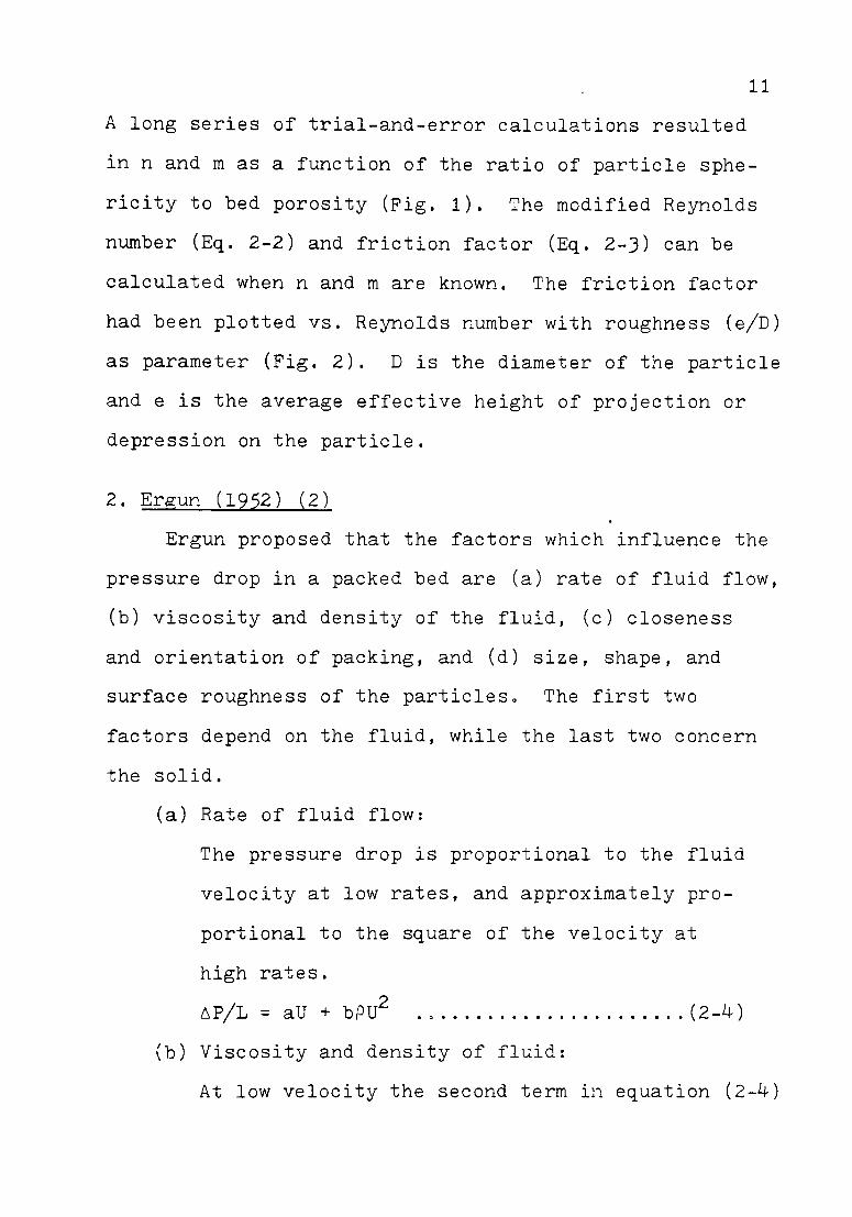
A long series of trial-and-error calculations resulted
in n and m as a function of the ratio of particle sphe
ricity to bed porosity (Fig. 1). The modified Reynolds
number (Eq. 2-2) and friction factor (Eq. 2-3) can be
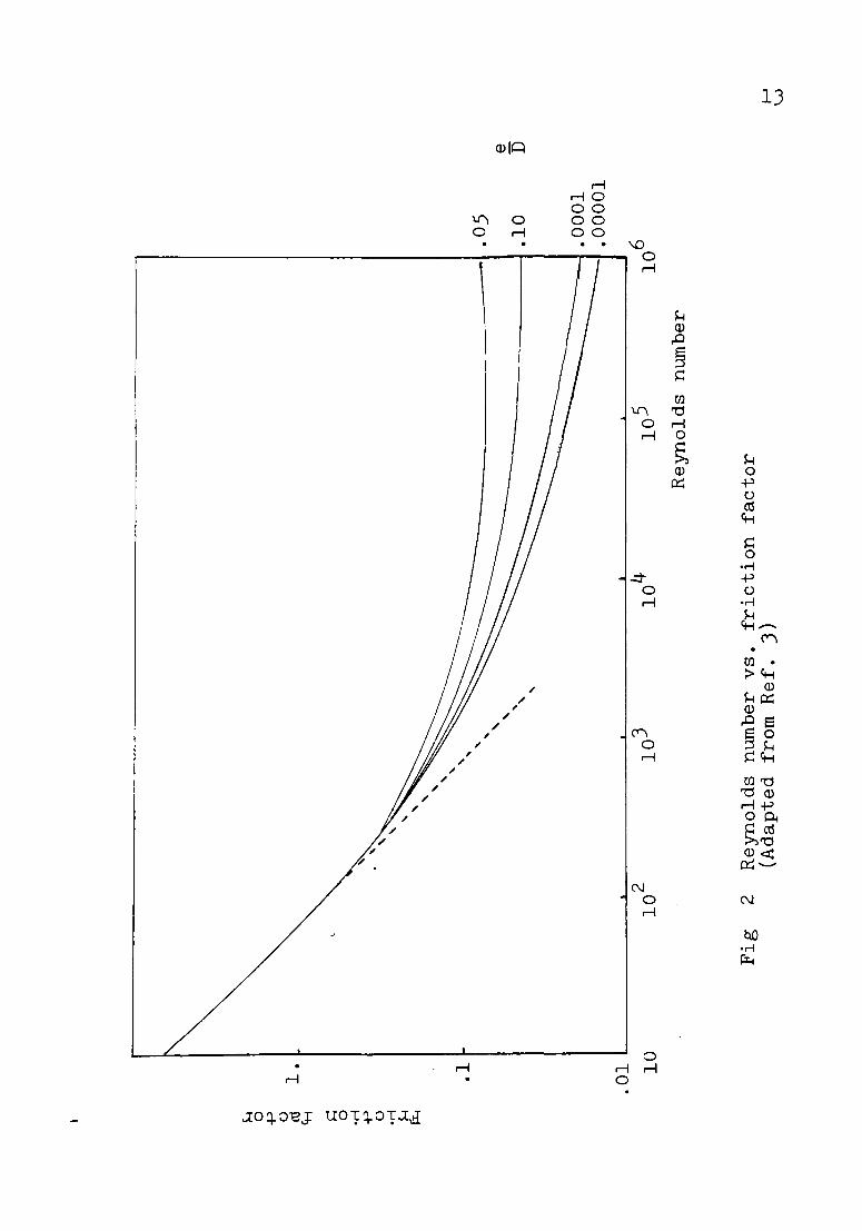
calculated when n and m are known. The friction factor
had been plotted vs. Reynolds number with roughness (e/D)
as parameter (Fig. 2). Dis the diameter of the particle
and e is the average effective height of projection or
depression on the particle.
2. Ergun (1952) (2)
Ergun proposed that the factors which influence the
pressure drop in a packed bed are (a) rate of fluid flow,
(b) viscosity and density of the fluid, (c) closeness
and orientation of packing, and (d) size, shape, and
surface roughness of the particles. The first two
factors depend on the fluid, while the last two concern
the solid.
(a) Rate of fluid flow:
The pressure drop is proportional to the fluid
velocity at low rates, and approximately pro-
portional to the square of the velocity at
high rates.
~P/L = aU + bPU2 ....................... (2-4)
(b) Viscosity and density of fluid:
At low velocity the second term 1n equation (2-4)

~
..p
•rl
[/) 0 H
0 Pi
H
0 'i-t
..p s:: Q
) s:: 0 Pi ~
rLI
30
20
10
5 4 3 2 1 o.
0.
5 1
.0
1.5
2
.0
2.5
3.0
3
.5
Fig
1
Ex
po
nen
ts
for
po
rosit
y fu
ncti
on
(A
dap
ted
fr
om
R
ef.
J)
sp
heri
cit
y
po
rosit
y
4.0
1--'
1\)
S--1 0 .p
() ro
1.
't-i ~
0 •rl
.p
()
·rl S--1
li-t
.1
' ' ' ' '
' ' ' ' ' ' '
' ' '
--------1
.05
------------~.10
.00
01
.0
00
01
.01~----------~----------~------------L------------L----------~
10
1
02
10
3
10
4 1
05
1
06
Rey
no
lds
nu
mb
er
Fig
2
Rey
no
lds
nu
mb
er v
s.
fric
tio
n fa
cto
r (A
dap
ted
fr
om
R
ef.
3)
e D
1--'
\....J

14
is not important and the first term is important,
which is a condition for viscous flow. In
viscous flow, the pressure drop is proportional
to viscosity. The pressure drop equation can
be rewritten:
.........••••.•.• (2-5)
(c) Closeness and orientation of packing:
Leva, et al. (31) stated that the pressure drop
was proportional to (l-E) 2/E3 at low flow rates
and to (l~E)/E3 at higher flow rates. With this,
the pressure
t-P/L = a"
drop equation 2
(1-E) ~u + b" E3
becomes:
1-E 2 p u I I I (2-6)
(d) Size, shape, and surface of the particles:
Ergun and Orning (32) proposed that the pressure
drop is proportional to the square of the
specific surface, Sv, in viscous flow and to the
specific surface at higher flow rates. The
pressure drop equation now becomes
t:-Pg /L = 2a~S 2u (l-E) 2/E3 + c v m
(13/8)GU s (l-E)/E3 ......... I (2-7) m v The particle diameter D = 6/S is substituted
p v
into equation(2-7) and the equation becomes
~Pg (l-E) 2 ~U (1-E)GU -~c =kl 3 m2+k2. 3 m ... (2-8)
1 E D - E D p p

15
Ergun concluded that the energy loss through a pack
ed bed can be separated into two parts, the viscous and
the kinetic energy loss. Viscous energy losses per unit
length are expressed by k1[ (1·-E )2/E3] [1-LU /D 2] and m p
kinetic energy losses are k2[(1-E)/E3] [GU /D ]. The m p friction factor f v' representing the ratio of pressure
drop to the viscous term takes the form
6-P D 2 E3 NRe f = p
kl + k2 (2-9) = v (l-E) 2 I I I I I I I
L 1-LU 1-E m Plot f vs. NRe/1-E from experimental data a solid line v
is obtained and the equation is
fv = 150 + 1.75 1-E ..................... (2-10)
Figure 3 is a logrithmic scale plot of the Ergun friction
factor.
3. Hicks (1970) (21)
Hicks proposed that the friction factor f of v
Ergun's equation is not a linear function of Reynolds
number. He suggested that in the range 300 < Re/(1-E) <
60, 000 the friction factor is ;,:ell represented by the
nonlinear relationship
f = 6.8 [Re/(l-E)]0 •8 v ' • • • • • • • • • • • • • • a • • • (2-11)
Parameters k1 and k2 of the linear Ergun equation
therefore vary with Reynolds number and are not truely
constant as is commonly accepted. Fig 4 is the compari-
son between Ergun's and Hicks' correlation.

16
..::t ...........
0 C\l 1""'1
' ct-; ~ (])
""' 0::: (]) \J)
.£ I s 1""'1 0
~ C"'1 ct-;
0 1""'1 '0
(])
~ Pi ro '0 <X:
...........
N (]) 0 0::: \J)
1""'1 ;;::: I 1""'1
rn :>
:> 0 ct-; 1""'1
C"'1
QD •r-i lit
1""'1 ..::t C"'1 N 0 0 0 1""'1 1""'1 1""'1
:> ct-;

N
"' .,-
.....
\1)
\1)
N
I P-
i rl
~
..........
. 0
;::::s
QD
:::t
P-i
<J
H
II :>
ct-i
50
00
00
10
00
0
50
00
10
00
~
A
Erg
un
's
Eq
uat
ion
,f'
/' "'
C!l
e•~
.. t·
'~C!) ~
/
/
:,A/
/
,·
" fl
" -
,e
" (-
]Hic
ks'
9G.4
E
qu
ati
on
C)
""\1
~,I(
J
~,
/
~
50
0
.. /-
+
10
0
.... 1
00
Fig
4
6
50
0
10
00
e W
entz
&
Tho
dos
(19
63
) e
Han
dle
y &
Heg
gs
(19
68
) •
Pec
k
& W
atk
ins
(19
56
) +
M
orco
m
(19
46
) Re
1-E
50
00
0
Co
mp
aris
on
b
etw
een
Erg
un
's
and
Hic
ks'
E
qu
ati
on
(A
dap
ted
fr
om
R
ef.
21
) f--
J --
...]

18
Two Phase Flow Pressure Drop
The manner of estimating pressure drop for two-phase
flow through packed bed can be separated into two major
approaches.
(a) Theoretical analysis but empirical correlation:
Larkins (1,4) considered each phase flow to be
through a section restricted by the presence of the
other phase. The two-phase flow pressure drop may
then be written in terms of the single-phase flow
pressure drop. Larkins used the parameter X defined
by Lockhart and Martinelli (29) to correlate the
pressure drop in two-phase flow through packed beds.
The solution is obtained by a theoretical analysis
but empirical means. Sato (16) and Midoux (8) used
the same parameter ;_ to correlate the two-phase flow
pressure drop.
Turpin and Huntington (15) used a momentum
exchange model (separated flow model) and assume that
each phase satisfied the conservation of momentum
separately and that the static pressures for each
phase are equal and constant at every cross section.
A "Z" group has been specificed as a function of
liquid Reynolds number and gas Reynolds number.
The friction factor is a cubic function of Ln (Z).
Hutton and Leung (7) presented a model in which
the two-phase flow pressure drop is a function of

19
gas flow rate in the restricted section of the bed,
and the liquid holdup is a function of liquid flow
rate and the pressure drop.
(b) Solving the modified flow model directly:
Sweeney (13) distinguished between the two
phases. He assumed that the liquid flows uniformly
over the packing surface, that both the liquid and
the gas phase are continuous, and that the pressure
drops through both phases are identical. The
fraction of void occupied by liquid is calculated by
trial and error and the two-phase flow pressure drop
is obtained by assuming single phase flow through
the void occupied by that phaseo
Clements (27) used a capillary model. The flow
in a packed bed is regarded as annular flow through
a bundle of capillary tubes. Surface tension is an
important factor in his model and the pressure drop
is a function of Weber number, liquid Reynolds
number, and gas Reynolds number.
1. Larkins (1959) (1,4)
Model:
During two-phase concurrent flow in a packed bed
each phase can be thought of as flowing in a bed
restricted by the other phase. The effective porosity
for one phase is reduced by the presence of the

20
second phase. The two-phase friction loss may then be
written in terms of the single-phase flow of liquid
in a restricted bed.
Assumptions:
1. The pressure drop for the gas is equal to that
of liquid phase and both pressure drops are
equal to the two-phase pressure drop.
2. hL is the liquid holdup, hGis the gas holdup,
E is the fraction void for the bed. Then
hL + hG = 1, and EhL and EhG are the effective
porosities for the liquid and gas respective-
ly.
The Reynolds number for the liquid may be defined as
••••••••••••••• 0 •• ( 2-12 )
The Fanning form of the friction factor is
J 2fL PL UL
(EhL)m D g p c
..................... (2-13)
The friction factor for the liquid may be expressed
in the general Blasius form as suggested for two phase
flow in pipes by Lockhart and Martinelli (29):
= [
Dll uL PL JJ ~L ( EhL)n
•.•..•...• (2-14)

21
Substitution of equation
~1 (Eh1)n = c 1 [____;;;;__-=--
Dp u1 p 1
2-14 for f 1 in 2-13 gives
3 2 PL u12 ] [---=--m~-] ..... ( 2-15)
( Eh1
) D g p c
~1 En 3 2 P1 u1
2
= c [ J [ J ns-m 1 Em D h1 •. (2-16) D u1 p1 p -p gc
The first two terms of equation 2-16 represent the
friction factor for the liquid flowing in the
unrestricted bed.
o - o h ns-m LG - 1 1 .................. (2-17)
The same procedure for the gas phase gives
oLG = oG (l-h1 )n's'-m' .................. (2-18)
Using equal exponents, that is, ns-m = n's'-m'
61 0.5
hG (s'n'-m')/2
h1 (m-sn)/2
X ( ) =[ J = = (sn-m)/2 -oG h1 (l-h1 )
............... (2-19)
The value of X can be calculated from an appropriate
single-phase correlation.
01G 1:. 2
Define ¢1 = ( o1
)
01G 1 2
and ¢G = ( oG
)
Further, it is observed that ¢1 , ¢G, and X are all
functions of the liquid saturation. Therefore, ¢1
and ¢G may be considered fQ~ctions of X alone.

22 1
0LG 2
.¢1 ( ) hL (sn-m)/2
Fl (X) .¢ G/x. . . ( 2 -2 0 ) = = = = 61 1
0LG 2
.¢G ( ) hG (s'n'-m')/2_F (X) - ¢ ..., .. (2-21) = = 6G - 2 - L'"
hL = F) (X) .............................. (2-22)
The value of .¢G becomes infinite as the gas rate goes
to zero and becomes unity as the liquid rate goes to
zero. In order to obtain a symmetric form for the
correlation, the definitions of .¢G and X may be
combined to obtain
= ........ (2-23)
Where F4 is a function which can be obtained from F1
or F2
•
So 6 LG is a function of X .
6 LG When log(o +6 )
1 G
is plotted against logX Fig. 5 results:
A curve fit gives the Larkins equation:
6LG Log 10 ( 6 +6 )
L G
Systems investigated:
0.416 = 2 ... (2-24)
[ (log10 X) + 0. 666]
Fluids used: water-air, methanol solution-air,
soap solution-air, ethylene glycol-
air, kerosene-natural gas, lube
oil-natural gas, lube oil-carbon
dioxide, hexane-carbon dioxide.

0 LG
oL+o
G
10
00
r-----
10
0
10
e A
ir-W
ater
a
Air
-Met
ho
cel
So
ln.
A A
ir-E
thy
len
e
Gly
col
oLG
0
.41
6
Log
lO(o
L+
oG)
(Lo
glO
X)2
+0
.66
6
h I
I ,,
l I
.AV
Y.,
1
I I ih
---
I 1 'o
X
Fig
5
Lark
ins'
co
rrela
tio
n
(Ad
apte
d
fro
m R
ef.
1,4
)
l\)
\.....
)

Packings used: J/8 in. Raschig rings, J/8 ln.
sphere, l/8 in. cylinders.
2. Sato (1973) (16)
The same model and assumptions as Larkins' corre-
24
lation have been proposed, but the symmetrical point is
%= 1.2 instead~= 1.0 as in Larkins' correlation. The
definition of 6LG is also different from what Larkins
used. Sato proposed that 6LG is the sum of static
pressure and the energy loss of elevation difference:
_.1_ + __Q_ + L + G
eeoo••••••••o•••(2-25)
·JL '2G
A curve fit glves the Sato's equation
System investigated:
Fluids used: air-water.
Packings used: 2.6 to 24 mm spheres.
J. Midoux, Favier and Charpentier (19?6) (8)
Correlations of pressure loss are proposed in terms
of the single-phase friction loss or frictional energy
for the liquid and the gas when each flows alone in the
bed. The parameters ¢Land z are defined as:
¢L = ( 6LG 6L
X ( 6L
= 6G
1 2
1 2
............................ (2-27)
) ............................ (2-28)

25 A curve fit glves .¢L as a function 0 f ~·~ .
.¢L = 1 + 1 + lol4 •••• 0 ••••••••••••••• (2-29) _, _, 0 0 54 I
/.
for 0.1 ~ X 80
The limiting cases are single phase flow of the liquid
phase and single phase flow of the gas phase,
G = 0, y_ = oo, .¢L = 1,
L = 0, " = 0, .¢L = 1/;','
Systems investigated:
Fluids used: water-air, cyclohexane-air, N2 ,
gasoline-N2 , He, co2 ,
petroleum ether-N2 , co2 ,
kerosene-air, N2 ,
desulfurized gas oil-C02 , air, He,
non-desulfurized gas oil-C02 , air, He.
Packings used: spherical catalyst 3 mm, glass sphere
3 mm, cylindrical catalyst 1.8 X 6 rnrn
and 1.4 X 5 mm.
4. Turpin and Huntington (1967) (15)
Model and assumption:
Momentum balances were written for each phase with
the assumption of a separated flow model. The total
pressure drop is expressed in terms of the sum of the
frictional pressure drop, the static pressure drop, and
the pressure drop due to acceleration of the fluids
(see figure 6).

gc(P+dP/2)dAL
DUE TO LIQUID PHASE AREA
CHANGE
/
g dF L C T
gc(P+dP/2)dAG
DUE TO GAS PHASE AREA CHANGE
--•• FORCE ----~-.~ MOMENTUM FLUX
Fig 6 Control surface for the momentum exchange model of Turpin and Huntington (Adapted from Ref. 15)
26

-(P - p ) = 2 1
For vertical flow e = 0, cos e = 1, and we can neglect
the acceleration term, so the equation becomes:
-(P2 - P1 ) = llPTPf + (1/A) (C 2AGL + PLALL + CJAGL2j2)
............ (2-31)
A area of flow
A the average area
Correlation:
The two-phase friction factor to be employed was
defined in the same manner as a single-phase friction
factor:
Where VGS is the velocity which the gas would have if it
were flowing in single-phase flow through the unpacked
conduit at the entering density PGl" D is the equivae
lent diameter which is four times the hydraulic radius
for the packed bed.
E
1-E ............... (2-.33)

28
For spherical particles: Vp/Sp = Dp/6, and
. . . . . . . . . . . . . . . . (2-34)
The results of a dimensional analysis of two-phase flow
with subsequent simplification shows the frictional
pressure gradient
~p
( 1 )TPf =
to be given
V2
GS PGl Ds gc
by:
•••••••oo(2-36)
Define z = N 1 · 167/N °·767 and use regresslon ReG ReC
methods to obtain
fTPf = 7.96 - 1.34 (Ln Z) - 0.0021 (Ln z) 2 +
0.0078 (Ln z) 3 . . . . . . . . . . . . . . . . (2-37)
0.2 ' 2 L 500
System investigated:
Fluids used air-water.
Packings used: 2,4, and 6 inches diameter columns
packed with tabular aluminum parti-
cles of 0.025 and 0.027 ft diameter.
5. Hutton and Leung (1974) (7)
Model and 2ssurnptions:
Assume both the liquid phase and the gas phase flow

29
continuously in the bed. Further assume that the liquid
holdup, h, in the column is dependent only on the liquid
rate, L, and the pressure gradient in the column,
(dP/dZ).
h = F1 (L, dP/dZ) ..................... (2-38)
The effects of gas flowrates on h are taken care of by
its effects on the pressure gradient. The pressure
gradient is assumed to be a function only of the gas
flowrate and holdup.
( dP ) dZ = F
2 (h,G) . . . . . . . . . . . . . ... (2-39)
The effect of liquid flowrate on ( dP ) is taken into dZ
consideration by its effect on holdup. The form of
equation (2-39) is taken as the same as the Ergun
equation for flow through packed beds using an effective
voidage available for gas flow defined as (1-c-h).
where c volume fraction occupied by solid
h liquid holdup per unit volume of column
Equation 2-39 can be written as
dP dZ = [
2 a GG v (
-G
~I a 0
·1
1 G v) J GG (l-c-h) 3
..•.•..•• (2-40)
Turpin and Huntington's experimental data were used in
developing this correlation.
6. Sweeney (196?) (13)
Model:
Assume two continuous phase are present 1n the bed.

JO The liquid phase flows uniformly over the packing surface
and both liquid and gas phase are continuous. The
pressure drops through both phases are identical.
Assumptions:
l. A pressure drop equation is available which
adequately predicts the frictional pressure drop
through the bed in terms of bed characteristics,
fluid properties, and fluid flow rates when
there is single phase flow in the system, that
lS, when the liquid or gas phase flows through
the bed in the absence of the other phase.
2. The pressure drop equation adequately predicts
the frictional pressure drop through the bed for
either phase when there is two-phase flow,
providing the presence of the other flowing
phase is taken into consideration.
Correlation:
From Ergun's equation for single phase flow:
4Pu2 6F = Ea + 4 a D~P J ............. (2-41)
gcD
The effective diameter and velocity are
D = 4 E (1-E) S
0 ' • • • • • • • • • • • • • • • • • • a • • • • (2-42)
-u = u
E . . . . . . . . . . . . . . . . . . . . . . . . (2-43)
Substitute (2-42) and (2-43) into (2-41) get
p~2 (l-E)S a~ (l-E)S0 oF= EJ 0 [~ + ] ••••• (2-44)
gc u )

Jl
Assume eL is the fraction of void volume occupied
by liquid, then
D = L
. . . . . . . . . . . . . . . . . . . . . .. (2-45)
. . . . . . . . . . . . . . . . . . . . . . . ( 2-46 )
Therefore, the frictional pressure drop through the
liquid phase is
PLuL2 (1-E)S 6' = 0 [~ +
LF eLJ EJgL
a.J.I.L(l-E)S --=---~0] • • • ( 2-47)
uL PL
Dividing by the value of oLF obtained for single
phase liquid flow from equation (2-41), one gets
6 , LF
6 LF =
1
e J L
........................ ( 2-48 )
Assume also a gas volume factor eG, so
. . . . . . . . . . . . . . . . . . . . . . . .. (2-49)
In this case, the velocity of the gas phase relative
to that of the liquid phase is - -UG UL
UG = 8GE 9LE
-UG y
eG E .......... (2-50) =
Where
y = 1 eGuL - ....................... (2-51) eLuG
Since the liquid is assumed to flow uniformly over
the surface of the packing, the number of packing
particles is the same as in single phase flow, but

32 the effective packing volume and surface area have
changed because of the presence of the uniform
liquid film.
Now define
and
(1-E)S z2 0
z = (1 +
so that
1 3
. . . . . . . . . . . . . . . . . . . . . . ( 2-52 )
) ..................... (2-53)
2 O.!J.G(l-E)S Z 0 J
uG p G y •• ( 2-54 )
Dividing by the value of oGF obtained for single
phase gas flow, one obtains
o'GF H =
6 eG 3
GF
Where $Y +
. . . . . . . . . . . . . . . . . . . . . . (2-55)
a.!J.G (1-E) s 0z2
H = yz2 [ uG PG J ... (2-56)
~ +
The total pressure drop through the liquid phase
is given by the combinations of friction loss and
fluid head terms for the liquid 0LF 6 'LT = 6 'LF- PL = 8G3
and, for the gas phase
phase:
. . . . . . . . . (2-57)
.33
6GFH 3
- p e G
G
. . . . . . . . .. (2-58)
It is assumed that the total pressure drop through
each phase is the same,
6 'LGT =
Since eL + eG = 1, therefore 1 1
0LF 3 6GFH 3 ( 6 1 LGT PL
) + ( 6 1 LGT ) = 1 .... (2-60) + + PG
To calculate the two-phase pressure drop, the following
procedure can be used:
1. Assume a value of eL
2. Calculate eG and H
J. Calculate a new value of eL from the relation
1 PL- PG 3
6 )]+1} ... (2-61) GF
4. Repeat steps 2 and 3 until a constant value of
eL is obtained.
5. Use equation (2-59) to calculate two-phase
pressure drop.
The modified form of equation (2-61) is assumed H = 1,
this form is to be preferred because of its simplicity. 1 1
3 + PL) J +
6GF [(6' + p )
LGT G J
3 = 1 •. ( 2-62)

34 System investigated:
Fluids used: N2co3 solution-air, CaC12
solution-air
and fluids used by Larkins et al.
Packings used: Berl saddles 1 in., lt in., tin.,
Intalox saddles 1 in., lt., tin.,
packings used by Larkins et alo
7. Clements (1980) (27,28)
Model:
Assume the packed bed may be treated as a bundle of
capillaries, each containing equal fractions of the
overall gas and liquid flows. The capillary dimensions
are function of the particle size, the bed void fraction,
and the particle shape; (Fig. 7)
Assumptions:
lo The frictional pressure drop contributions of
the liquid to the overall pressure drop are
negligible.
2. Neglect gravity effects in the liquid phase.
J. The overall pressure drop across the region of
interest is low enough that gas phase properties
may be taken as averages of entry and exit
values.
4. No slip at the gas-liquid interface.
5. At any point, Z, there is axial symmetry.
With these assumptions the liquid equation of motion is

35
...-... CX)
'0 C\l .,..; ::s t::r
.,..;
.
.....:l
('-
-r
r-1 C\l
H
Q)
~
'0 •
t 0 Ii-i s ~ ~ s
(/)
~ 0
ro
ro ~
eJ
r-1'+-i r-1 .,..; '0
()
P..Q)
~
ro~ () p..
'0
a> ro ..c:'O 8.::s .,..;
_L ::s t::r
.,..; .....:l
C'-
QD .,..; li-t

36
o UzL PL uzL ( o z ) =
-IJ.L o auZL r [ o r (r a r ) J · · · · · (2-63)
Let 3 = Z/L
-rr = r/R
uL= uzL/m/n(R2- ri2) PL
to get the dimensionless expression
l l o o UL R~ L [ ( -17- a.;) ( '7 o. -ry ) J . . . . ( 2- 64 )
Where 2 2 2 = ~ /[ nL(R - r 1 ) IlL]
For the gas phase
=
Therefore,
v1here
- (
aP
az
. . . . . . . . . . . . . . . . .. (2-66)
If we require that a equilibrium exist at every point 1n
the capillary between the pressure exerted by the gas
phase and the restoring surface force exerted by the
liquid phase.
P (Z)gas = [a/rr(Z)] liquid . . . . . . . . . . . .... (2-68)
Taking derivatives of this equation
aP =
- o o r 1 -~2 ( ) ····················· (2-69)
r 1 o 3

37
Substitution of equation (2-69) into (2-67)
a 1 1 a UG a ri a uG UG ( a l'j ) = -A a ! - ReG
-( ~1') a 1': ) •• (2-70) 'I] I
where
The liquid holdup is
Ho = (R2- ri2)/R2 .......................... (2-71)
So, a ri R2 a H a ~ - - 2r I ( a ~ 0
) . . . . . . . . . . . . . . . . . . (2-72)
And equation (2-70) becomes
1
we G
It is assumed that
ReGWeG
a H 0
a n J
1 1
p~G -Y!-o a uG
[ a1J (11 a Yl ) J ......... (2-73)
H = f ( 0 ReL ) . . . . . . . . . . . . . . . . . . . . . . . (2-74)
From the assumptions, the two-phase flow pressure drop
must equal to both gas and liquid single phase pressure
drop, therefore
- ( ~p 6P ~p I
~L )TP = - ( ~L )G = - ( ~L )L = (Wf P)TP ......... (2-75)
From the Blasius form of the friction factor
and from the Brownell and Katz friction factor
n/ 2 fG = 2~PG DPEG ~LuG . . . . . . . . . . . . . . . . . . . .. (2-77)

Eliminate fG
(Wf P)TP
from equation (2-76) and (2-77)
= CG [
= c [ G
IJ.G(EHG)m s pGuG
2
J [ J Dp PG 2(EHG)nDPgc
II -cffi S 2 ~G ~ J [ _PG;;;._.u...;;;.G __
DPPG 2EnDPgc
(ms-n) J HoG
38
= WfG (HoG)-x . . . . . . . . . . . . . . . . . . . . (2-78)
There ( 6P )LG/( 6L
From the silicone-air two phase flow experimental data
Clements and Schmidt (27) obtained the expression
( 6p ) /( ~p )G = 190 D ( 6L LG 6L UL P
. . . . . ... (2-80)
System investigated:
Fluids used : air-silicone oil.
Packings used: Sphere 1.6 mm, 3 mm.
Extrudate 0.8 mm.

CHAPTER III
THEORETICAL ANALYSIS
Energy Balance
The general energy balance in a flow system is
2 J VdP + ~u + ~z· + wf + w = o ......... (3-1)
gc s
where v is the specific volume per unit weight, u is the ~u
2 velocity, 2g lS the kinetic energy difference due to
c changes ln velocity, z is the vertical distance and ~z
indicates the potential energy difference, wf is the
energy converted into heat by friction, and W is shaft s
work done on the surrounding by the system. W lS zero s
for two-phase downward flow. The velocity difference is
usually small over the column.
( velocity = volume flow rate/cross section area,
volume flow rate = liquid mass flow rate
liquid density
+ gas mass flow rate
gas density
In the flow system liquid mass flow rate and gas mass
flow rate are constant either on the top or bottom
section. The density of liquid is constant, but the
gas density varies with pressure. So, if the column
is short, the pressure difference is small, and we may
gas density varies only slightly.
term is very small.)
39
Hence the

Equation (3-1) can be written as
J VdP + ~z· + wf = 0 . . . . . . . . . . . . . . . . . . . . . . Using specific volume V as the inverse of specific
density
1 v = Pm
Equation (3-2) becomes
. . . . . . . . . . . . . . . . . . . . . . . . . . . . . . . .
40
(3-2)
(3-3)
~ __ dP + ~z' + w f = o . . . . . . . . . . . . . . . . . . . . . . . . ( 3-4) m
Assume p is constant and integrate the first term, m
~P + ~z· + wf = o m
. . . . . . . . . . . . . . . . . . . . . . . . . . . . Divide by ~Z and rearrange
• 0 • • • • • • • • • • • • • • • • • • • • • • • • ••
Let ~Z'= -~Z (change sign because we want downward
direction to be positive)
. . . . . . . . . . . . . . . . . . . . . . ..
(3-5)
(3-6)
(3-7)
is the measured pressure drop per unit length over
the column.
~p + p - ~z m ••••••••••••••••••toot {3-8)
oLG is the total energy required to overcome friction
per unit length downward through the packed column.
Larkins ( l, 4), and Turpin ( 15) regard Pm as h P1 + ( 1-h) PG,
where h is the liquid holdup. Sato(l6) regards p as m
(L+G )/ (1/ P1 + G/ PG). In this correlation pm is equal to

41
(L+G )/(L/ .-·1 + G/ ... G), because the specific volume per unit
weight is
V = (~ + ~)/(L +G) __,L ~""G
and ~m is the inverse of V (Eq. 3-3).
Model
In this development, two models are considered. The
first one is the capillary flow model describing viscous
flow and the second one is a capillary seperation flow
model describing kinetic flow.
1. Viscous flow
Capillary flow model: (Fig 8)
Treat the packed column as a bundle of capillary
tubes. The liquid flows laminarly along the wall of the
capillary and the gas also flows laminarly through it in
the center.
The diameter (D ) of the capillary is assumed to be c
equal to the effective diameter, De' of the packing.
D = D = effective diameter c e = 4 wetting volume/ wetting area
= 4 E/(6(1-E)/Dp) 2 E
= 3 Dp ( 1-~ )
The equation of motion for both liquid phase and gas
phase is
~L (--a--(r a uzL)) r or a r
a P az .•..• (3-9)

/ 42
D c ' ' ~I '
Liquid Gas Liquid " " L G L
wall wall
' " ' " ' '
~ I v I
I
I
I v I
I
I
" I v I v ' ~ .. ...... w,... v
velocity profile
Fig 8 The capillary flow model

Assume the vertical velocity gradients are zero, although
gas density is different for the top and bottom section
and the velocity is also slightly different. The
equations become
~1 a a ---r- (-ar (r a
a P az
~G ( a (r a uzG)) = r ar a r
a P a---z
B. c. 1 r=r uz1=o c
B. c . 2 r=r I Uz1=uzG
B. c . J r=r I -r1=-rG
B. c. 4 r=O -r -o G-
............... (J-11)
··············· (J-12)
To solve equations (3-11) and (J-12)
define ~ r = r c
* * u - uzG/(G /PG) G-
* * u = uzrl (1 I P1) 1
* Z/rc z =
* G = mass flow rate of 2 gas lb/ft .hr
* of liquid lb/ft2 .hr 1 = mass flow rate ~~ ..
P/Patmosphere p =
The dimensionless forms of Equations (J-11) and (J-12)
are * aP ~ az
·············· (J-13)

44 * aP ~ az
............. (3-14)
B. C. 1 3=1
B. C. 2 * L i .. G UL = UG
PG PL ·n· *
B. C. 3 IlL L auL PLaT
= !lG G auG PG aT
B. C. 4 3=0
* * 2 EuL is the Euler's number of liquid, P atm PL/ (L )
* * 2 EuG is the Euler's number of gas, p atm PG/(G )
* * ReL is the Reynolds number of liquid, L De/IlL
* * ReG is the Reynolds number of gas, G Dc/!lG
* * * EuL ReL Define KL=
ap ---:'i' 2 az
* * * EuG ReG and K =
ap G * 2 az
Substitute KL and KG into Equations (3-13) and (3-14),
and integrate twice to get
* 1 32 UL = 4 KL + cl Ln 3 + c2 ............. (3-15)
and
* 32 3 u - 1 KG + C3 Ln + c4 G - 4 ............. (3-16)
Apply B. c. 4 to get c =0 3
Apply B. c. 3 to get c =0 1 Apply B. c • 1 to get C2=-iKL

45
Substitute c1 , c2 , c3 , and c4 into Equations (J-15) and
(J-16) to get
The
gas
U ~ = i K1 ( ~ 2
-1 ) . . . . . . . . . . . . . . . . . . . . . . . . . . ( J -1 7 )
conservation of mass equations for both liquid and
are . . * r
Liquid: 1 2 =! c u12'1"JT dr I I 1 1 1 1 I I I 1 I I I I I (J-19) - nr P1 c ri
Substitute UL into (J-19) and the equation becomes
t = ..................... {J-20)
Substitute (J-17) into (J-20) to get 1
t = J s i K1 ( ~ 2 -1 ) ~ d ~ . . . . . . . . . . . • ( J-21 )
Integrate (J-21) to get
2 KL
= -i
Solve (J-22) to get
2 -8 )t s = 1 - (~-KL
................. (J-22)
................... (3-23)
K1 is negative by previous definition, and S is
always less than 1.
* G 2 Gas: -- nr PG c
ri = !0
uG 2nr dr ................ (J-24)

46
Substitute uG into (J-24) and the equation becomes
* s 2 2 2 L PG t= /
0 [iKG~ -iKGS +iKL(S -1) * ]~ d~ ... (J-25)
G PL Integrate (J-25) to get
* 1 l 4 l 4 l L PG 2 2 2 =f6KG S - 8KG S + 8KL ( -lt- ) S ( S -1 ) ...... , ( J- 2 6 )
G PL
From the definitions of KL and KG the following
expression can be obtained
* f.l.G G PL
* ...................... ( 3-2 7)
f.l.L L PG
Substitute (J-27) into (J-26) to get
f.J.L is usually much greater than f.J.G' neglect the
smaller term to get
! = s4(- ftKG ) - ~KGS2 ~~ ............. (J-29)
Substitute s2 (J-2J) into (J-29), and neglect the
smaller term to get
1 KG l l ( - 8 ) t t = 2 K - IbKG + 8KG K
L L ............ (J-JO)
Define w=KG/KL and substitute into (J-JO) to get
t = ............. g.(J-31)
Solve (J-Jl) to get l.
-KL = 8 + 8/w + l6/w2 .•...........••.•.• (J-32)

47
From the preVlOUS definitions
* i}
* Eu1 Re
1 D iJ -KL=
aP ap c L i~
~ = - Re1 ooooo(3-33)
az 2 az (L~l-)2
so,
•o•••••••••••••••••(J-J4)
Substitute
* Re 1 = Rer/(1-E)
De=Dc= ~ DpE/(1-~)
* L = L/E
...... (3-35)
From this mathematical model, the two phase concurrent
flow pressure drop equation has the following form,
0 ...... (3-36)
1n the viscous flow portion. The coefficients A1 , A2 ,
and A3
are constants.
2. Kinetic flow
Capillary separation flow model: (Fig. 9)
In the turbulent flow region, the fluids are
considered to flow in a separation flow model, that 1s,
the liquid phase and the gas phase flow separately. In
the center of the capill~y tubes, the liquid and gas
flow at the same velocity u1 . Near the wall of the

A. Partial capillary separation flow D
velocity profile
~
L
J
*
R
~
c
Liquid
G*
1r Gas t Liquid
Gas I r1-~t
'
B. Total capillary separation flow
velocity profile
u II
Liquid
Gas
Liquid
Gas
, ,
L~ t * ~ G "
L ~
,
¥
u
ull=
II
Fig 9 The capillary separation flow model
48

49
capillary tubes, the liquid flows along the wall with
velocity u2 , and the thickness is t. When both the gas
and the liquid flowrates are too low, the amount of liquid
in the center is very small and this is the capillary flow
model. When both the liquid and the gas flowrates are
high enough, u2 is very small compared to u1 , and the
thickness near the wall is very small too. Under this
assumption, the liquid and the gas will flow at the same
velocity u".
Lerou, Glasser, and Luss(22) used this model to
describe the pulsing flow. Originally this model was
used to study the effect of axial dispersion. Here, the
pressure drop effect is of interest in this model.
For the partial separation model, assume the liquid
flows laminarly near the wall. The velocity profile
in a tube for laminar flow is
oF R2 1-( r )2] uz = - az 4u
1 [ R ........... (3-37)
at r=r 1 * *
u" _1_+ G uz = ul ~ =
PG PL so,
2 (u ) = - oF .JL [l-(Rr)2] ~ u" ....... (3-38)
z 1 az t.ru1
rearrange and multiply by L2P1 /L2P1
aF az =
u" 4u1
R2[1-(r1/R) 2J

2 ~ QLU" 2 =(4L _1 L )/[1-(rl/R) J
PLR RL
= 72(1-E) 2L2
E2
PLDpReL
50
1 ... (3-39)
G PL . LP ls much greater than 1 and r 1 is nearly equal to R,
G
so Equation (3-39) can be rewritten as
The thickness of the liquid, t, increases when the liquid
volumetric flowrate increases or the gas volumetric flow-
rate decreases. From this we can say that t is a
function of G 9r/L ~h.
Equation (3-40) becomes
Define
ap az
The Reynolds number of
D u"P " ReL = e L ~L
=
............ (3-41)
................ (J-42)
the liquid at the center is @
2 ReL
3 1-E ................. (J-43)
The pressure drop caused by gas friction lS small

51
compared to the pressure drop caused by liquid friction.
So, the gas term has been neglected. The pressure drop
ln a turbulent flow is proportional to the n-th power
of the Reynolds number, based on
Re@ _ oP ot:.R "nat..( L )n az eL 1-E
Combine (3-41) and (3-44) get
Taking
oP az =
boundary layer theory.
............... (J-44)
GPL LP ) ••••• ( 3-4 5)
G
= ( !::.ZP) . + ( ~zp) k. t. . .... ( 3-46) !::. VlSCOUS u lne lC
At laminar flow (6P) is very small compared t::.Z kinetic
to (~~)viscous and Equation (3-36) is equal to (~~)TP'
At turbulent flow,
t::.P to (AZ)k. t· and
u lne lC
(~2P) . is very small compared u VlSCOUS
Equation (3-45) is equal to (~~)TP"
In the transition zone, both (~~)viscous and (~~)kinetic
are important.
Combine (3-8), (3-36), and (3-45) get
The constants A1 , A2 , A3
and the function F will be
determined in Chapter IV.

CHAPTER IV
CORRELATION AND DISCUSSIONS
Data Characteristic
Experimental data from four investigators have been
used in developing this correlation. Larkins(4) collected
his data in 1959 for his Ph.D. dissertation and 555 data
points have been used from his data set. Clements(27) col
lected silicone oil-air data in 1975 for Chevron Research
Company and 279 data points are used from his report.
Halfacre(26) collected his data in 1978 for his Master's
thesis and there are 531 data points listed in his thesis.
Weekman(25) collected his data in 1963 for his Ph.D. dis
sertation and there are 183 data points used. Turpin(30)
collected some data in 1965 for his Ph.D. dissertation.
His data were not included because the calculated single
phase pressure drop from Ergun's equation is higher than
experimental two phase pressure drop.
In all, there are 1570 nonfoaming data points which
have been used in developing this correlation. Table III
shows the characteristic parameters of these data.
52

Tab
le
III
Ch
ara
cte
rist
ics
of
Tw
o-P
hase
P
ack
ed
Bed
P
ress
ure
D
rop
Dat
a U
sed
Dat
a S
ou
rce
Sy
stem
P
ack
ing
D
iam
eter
Vo
id
Am
ount
L
iqu
id
Liq
uid
S
et
ft
Fra
cti
on
o
f D
ata
Vis
co
sity
D
en
sity
cp
lb
/ft3
1 C
lem
ents
S
ilic
on
e-A
ir
Sp
her
e 0
.00
52
0
.38
8
42
1.3
9
53
.5
2 C
lem
ents
S
ilic
on
e-A
ir
Spfi~re: · ~
-0
.00
52
0
.38
8
45
4
.62
5
7.6
3 C
lem
ents
S
ilic
on
e-A
ir
Spflere~·
0. 0
096
0.3
18
8
7
4.6
2
57
.6
4 C
lem
ents
S
ilic
on
e-A
ir
Ex
tru
date
0
.00
34
0
.36
1
36
1.3
9
53
.5
5 C
lem
ents
S
ilic
on
e-A
ir
Ex
tru
date
0
.00
34
0
.36
1
69
4
.63
5
3.5
6 H
alf
acre
W
ater
-Air
S
ph
ere
0.0
2
0.3
7
93
0.8
9
62
.l2
7 H
alf
acre
W
ater
.IP
A(3
%)
Sp
her
e 0
.02
0
.37
Z
4 1
.0
61
.5
-Air
8 H
alf
acre
W
ater
.IP
A(4
%)
Sp
her
e 0
.02
0
.37
54
1
.05
6
1.4
-A
ir
9 H
alf
acre
W
ater
.IP
A(9
.5%
) S
ph
ere
0.0
2
0.3
7
39
1
.34
6
0.8
-A
ir
10
H
alf
acre
W
ater
.IP
A(l
l.5
%)
Sp
her
e 0
.02
0
.37
42
1
.46
6
0.8
-A
ir
11
H
alf
acre
W
ater
.IP
A(2
0%
) S
ph
ere
0.0
2
0.3
7
33
1.9
5
59
.9
-Air
\...
1\
\..U

Tab
le
III
(co
nti
nu
ed
)
Dat
a S
ou
rce
Sy
stem
P
ack
ing
D
iam
eter
Voi
d A
mou
nt
Liq
uid
L
iqu
id
Set
ft
Fra
cti
on
o
f D
ata
Vis
co
sity
Den
sity
cp
lb
/ft3
12
Half
acre
W
ater
.IP
A(4
8%
) S
ph
ere
0.0
2
0.3
7
42
2. 9
8 5
6.1
-A
ir
13
H
alf
acre
W
ater
.IP
A(4
%)
Sp
her
e 0
.01
0
.34
1
5
1.0
5
61
.4
-Air
14
H
alf
acre
W
ater
.IP
A(9
%)
Sp
her
e 0
.01
0
.34
27
1
.34
6
0.9
-A
ir
15
H
alf
acre
W
ater
.IP
A(l
9.5
%)
Sp
her
e 0
.01
0
.34
42
1
.94
6
1.4
-A
ir
16
H
alf
acre
W
ater
-Air
S
ph
ere
0.0
1
0.3
4
54
0.8
9
62
.12
17
H
alf
acre
W
ater
.IP
A(4
8%
) S
ph
ere
0.0
1
0.3
4
54
2. 9
8 5
6.1
-A
ir
18
H
alf
acre
W
ater
.IP
A(1
.5%
) S
ph
ere
0.01
1 0
.34
1
2
0.9
1
61
.7
-Air
19
W
eekm
an
Wat
er-A
ir
Sp
her
e 0
.02
12
0
.43
62
0
.9-1
.0
62
.4
20
Wee
kman
W
ate
r-A
ir
Sp
her
e 0
.01
55
0
.39
56
0
.9-1
.0
62
.4
21
Wee
kman
lr
J2.t
er-A
ir
Sp
her
e 0
.01
24
0
.37
8
65
0.9
-1.0
6
2.4
22
Lark
ins
Wat
er-A
ir
Ras
chig
0
.01
94
5
0.5
2
272
1.0
6
2.4
R
ing
\..
J\
+=-

Tab
le
Data
S
ou
rce
Sy
stem
P
ack
ing
S
et
23
L
ark
ins
Meth
ocel
So
lu-
Rasc
hig
ti
on
-
Air
R
ing
24
L
ark
ins
Eth
yle
ne
Gly
co
l R
asc
hig
-A
ir
Rin
g
25
L
ark
ins
Eth
yle
ne
Gly
co
l S
ph
ere
-A
ir
26
L
ark
ins
Wate
r-A
ir
Sp
here
27
L
ark
ins
Wate
r-A
ir
Cy
lin
der
28
L
ark
ins
Meth
ocel
So
luti
on
Cy
lin
der
-Air
29
L
ark
ins
So
ap S
olu
tio
n
Cy
lin
der
-Air
IPA
:
Iso
pro
py
l A
lco
ho
l
III
(co
nti
nu
ed
)
Dia
mete
r V
oid
A
mo
un
t L
iqu
id
Liq
uid
ft
Fra
cti
on
o
f D
ata
V
isco
sit
y D
en
sity
cp
lb
/ft3
0.0
19
45
0
.52
5
4
12
.0-1
4.0
6
2.4
0.0
19
45
0
.52
6
5
12
.0-1
7.0
6
9.5
0.0
31
25
0
.36
2
62
1
2.0
-17
.0
69
.5
0.0
31
25
0
.36
2
. 4
4
0.8
-1.0
6
2.4
0.0
10
4
0.3
57
3
4
0.8
-1.0
6
2.4
0.0
10
4
0.3
57
1
2
2.0
-2.9
6
2.4
0.0
10
4
0.3
57
1
2
0.8
-1.0
6
2.4
\..n
\.
.n

56 Correlation of Experimental Data
It is the objective of this section to find out what
coefficients(A1 , A2 , A3
) are and what function F is in
equation(J-47). To achieve this, assumptions and preliminary
calculations must be made.
1. Assumption
1. No mass transfer between the liquid and gas phase,
so that the liquid flow rates and gas flow rates
remain constant.
2. No heat transfer from the surroundings and no heat
transfer between the two phases, so that throughout
the column the temperature is constant and liquid
temperature is the same as gas temperatureo
J. The gas density is assumed to be constant in the
column. The density is calculated at the average
pressure between two measured points.
4. The velocity along the column is constant for both
liquid and gas phases.
2. Preliminary calculation
lo Calculate the experimental average pressure
pav = (Ptop + pbottom)/2
2. Calculate the average gas density
:·hav = p avM/RT
J. Calculate the true pressure drop
0LG =-( ~~)observed+ (L+G)/(L/~L + GjpG)

57 3. Correlation
Equation(3-47) is the basic form of two phase flow
pressure drop. Define friction factor fTP as
fTP=6LGt:3 r-L DPReL/ (L 2 ( 1-E) 2) .............. ( 4-l)
combine (3-47) and (4-l) get 1 GP1 fTP=A1 + A2/w + A3/w2 + F(Re1@/(l-E), JGL) .. (4-2)
fTP= fv + fk ............................. (4-3)
fv: Viscous friction factor 1
= A1 + A2/w + A3/w~ fk: Kinetic friction factor
G~ = F (Re1@/(l-E), , ~)
:"G Kinetic portion:
In turbulent region fv is very small compared to fk.
fk is a function of Re1@ and G?1/JGL and we will empirically
determine what this function is in this section.
From equation (3-~)
- :~ e£ (Re1@/(l-~) )n .................. (3-43)
So, in turbulent flow region
fTP=fv + fk ~ fk o-: (Re1@/(l-~) )n .......• (4-4)
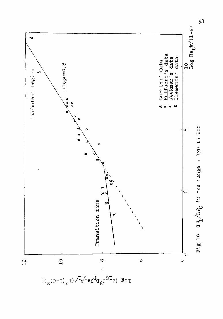
Fig. 10,11,12,13 are plots of the calculated results from
the data. The calculated values of Log(fTP) are shown
plotted against Log(Re1@/(l-~)) at constant volume ratio
( GP1/ PGL).
For higher values of Re1@/(l-E) the graph is linear and
the slope is 0.8. In fig. 10,11,12,13 the volu~e ratio is
different but the slope is the same. So, in turbulent flow
.........
.........
N ,....
.., \J
) I rl
....,.
C\J t--=
1 ....
,. "'-
-.. t--=1
0..
t--=1
Q)
~
~P-t
C'\
\J
) CJ H
<0
....
,. QO
0 t--=1
12
10
Tra
nsi
tio
n
zon
e 8
" "'
/
/ ;
; ,
/
·'
, 6
/
/
4 4
6
Fig
10
G
PL
/L P
G in
th
e
ran
ge
• •
A
n/
o
0
8
17
0
to
200
Tu
rbu
len
t re
gio
n
A
slo
pe=
0.8
A
Lark
ins
' d
ata
0
Half
acre
's
data
•
Wee
kman
' s
data
X
C
lem
en
ts'
data
·10
6
Log
ReL
@/(
1-E
)
\..n
(X)

,-..
. ,-
...
N ,-
...
\J) I
r1
....._..
N H
.._
_. "'-
.. H
0..
H
Q) ~
C'\
\J
) 0 H
c.O
.._
_. QD
0 H
12~----------------------------------
10
8
4
Tra
nsit
ion
zo
ne /
/
/ /
/
/
A o o~-·
0 ty
0
'/..
/,.,
,..
0 0
/ 0
Fig
ll
G P
L/L
Pa
in th
e
ran
ge
0 ll
0 0
90
to
11
0
Tu
rbu
len
t
slo
pe=
0.8
A
Lark
ins'
data
o
Half
acre
's
data
•
Wee
km
an's
d
ata
X
C
lem
en
ts'
data
Lo
g R
eL@
/(1
-E)
\.n
\.
()

,--.
.. ,-
-...
N ,.-
....
w I r-1
.........
N .....
:! .....
.... ~
a... .....
:! Q
) p:
; ~P-i
(Y
"'\ w 0 .....
:! cO
.....
.... b.O
0 .....:!
12~----------------------------------
Tu
rbu
len
t re
gio
n
10
0
• A
bP
A
o
. 0
__
,-0
Tra
nsi
tio
n
zon
e •
81-
~,
~ A
,,
p
d
" t
'I. ~
0 ~"
0 /
" /
/
/ /
6~
/ /
, /
A
Lark
ins'
d
ata
0
Half
acre
's
data
•
Wee
kman
's
data
t
Cle
men
ts'
data
I
4 4 6
8 10
@
L
og R
eL
/(1
-E)
Fig
1
2
G P
L/L
Pa
in th
e
ran
ge
. 40
to
50
~
. 0

,........
.,........
N
.,........
\1
) I rl
......_..
..
N ....
:! .....
._....
12
r---------------------------------------------
Tu
rbu
len
t
~
10
dA
A
A
Q ....
:! Q
)
p:::;P
-t j:
:l
(Y\ \1
) 0 ....:!
<0
.....
._....
till
0 ....:!
Tra
nsit
ion
zo
ne
8 4
l ~ A
•
A o
-- 9 .b
V4
/ 0
,. ..
/
6 /
/
/ ,
, /
/
A
A
AA
4
4 L
ark
ins'
data
o
Half
acre
's
data
•
Wee
km
an' s
d
ata
X
C
lem
en
ts'
data
4 I
4 6
Fig
1
3
G(J
L/ P
aL
in
the
ran
ge
8
?.5
to 1
2.5
10
L
og
ReL
@/(
1-E
) 0'.
f-
J

62 region the friction factor fk is a linear function of
(Re1@/(l-E)) 0 · 8 • This correlation matches with Hick's(21)
correlation for single phase pressure drop through a
spherical packed bed, the power of Re/(1-E) is also 0.8 for
turbulent flow. It is easy to see that for turbulent flow
Re1 @
0.8 GP1 f - ( ) Fk( (fL ) •• I I • e e e e I e • I I I I ( 4-5) k- 1-E 0
G
In Fig. 10,11,12,13 the transition point is at @ h @
Log(Re1 /(1-E)) about equal to 7, that is, Re1 /1-E ~ 1100.
The liquid flow is turbulent when Re1@ / (1-E) > 1100. When
Re1@/(l-E) ~1100 the flow is in transition zone or laminar
flow. To distinguish between the laminar flow and the @
transition zone is very difficult, because for Re1 /(1-E)
< 1100 two conditions can exist: (1) the liquid flow is
la~inar and the gas flow is turbulent (2) both the liquid
flow and the gas flow are laminar. In the first condition,
the flow is in the transition zone. In the second condition,
the flow is described by the capillary flow_model. an~ w~is
the important variable. It is very difficult to say at what @
value of Re1 /(1-E) the capillary flow will truly fit the
flow.
Fig. 14 and 15 are plots of Log(fk/(Re1@/(l-E)) 0 ' 8 ) vs.
Log(Gp1/pGL). Fig. 14 is a plot for both spherical and
cylindrical packings. Fig. 15 is a plot for Raschig ring
packings. Both curves are hyperbolic curves. For Raschig
ring packed beds, the geometry of the particle is less
smooth and it causes higher pressure drops. Accordi!}:g-to

5 .,
-...
I I<D .
0 .,
-...
.,-
...
\J.J
P,l I
4 8
8
G-i
"'- @ t--=
1 <
I)
IX:
1-- -- t:U
J 3
0 t--=1
2 1
'I. •
){
:>e ......._
. 0
0 0
• 0
0
0 0
o o
o o
• )(
oo
oo
o
• 0
0
0 1
2 3
Fig
1
4
Sp
heri
cal
and
cy
lin
dri
cal
pac
kin
gs
4
!J L
ark
ins'
d
ata
o
Half
acre
's
data
•
Wee
kman
's
data
t
Cle
men
ts'
data
0 0
0 0
0 0
• 0.
• oo
/
0 ;:.
..---
0
41 0 5
0
6
Lo
g
r('G
pL/L
PG)
~
I.....V

ct1 ~
+'I ct1 '0
00 ~
•rl ~
S-.1 ct1 H
( e·o< (3-T)/©'IaH)
dili~ ) ~0'1
'1.1\
C\l
0 ~
64
.,-.... ~
a.
~ o..H ~ ...........
QD 0 H

Larkins' (4) correlation, the friction factor is different
for different packing shapes when calculating the single
phase pressure drop. After regression, the best fits for
the curves in Fig. 14 and 15 are:
For spherical and cylindrical packings:
65
GPL 2 Log Fk= 1.60+0.109(Log(p L)-2.9) ................ (4-6)
G
Substitute into Re @
(4-5)
f = ( L )0.8 k 1-E
GPL 2 . Exp(l.60+0.109(Log(p L)-2.9) ) ... (4-7)
G
For Raschig ring packing:
GPL 2 Log Fk= 2.10+0.109(Log(p::y;)-2.9) ................ (4-8)
G
Substitute into R @
(4-5)
f = ( eL )0.8 k 1-E
GPL 2 • Exp(2.10+0.109(Log( p L)-2.9) ) ... (4-9)
G
Viscous portion
For the laminar flow region, w is the most important
group which influences the pressure drop. w is defined as _.1..
(LPGuL)/(PLGuG). Fig. 16 is a plot of fv vs. w 2 for
ReL@/(1-E) less than 50. Since there are no Raschig ring
packing low Reynolds number data, the viscous portion cannot
be correlated.
For spherical packings:
fv = fTP - fk ••................................. (4-10)
fTP is calculated from equation (4-1)
fk is calculated from equation (4-7)
The curve in Fig. 16 is hyperbolic. After regression, the
following equation was obtained.

f v
Th
is co
rrela
tio
n
10
00
L
-----
Th
eo
reti
cal
valu
e
'I.
500
30
0
--, __
_
0 0
o.s
Fig
16
@
R
eL /(
1-E
) le
ss
than
50
1.0
y.
,;
, ~
,.
,. ,
.... .,. - t C
lem
ents
' d
ata
1.5
1
( G P
Lf! c
/L p
Gil
L)
2
~
~

1 fv = 300 + 240/w + l20/(w2) It I 1 1 1 I I I I I I I I I It (4-11)
The theoretical value of fv for capillary model (3-35) is 1
fv(theoretical) = 72 + 72/w + l44/(w2) 00 0. ooo (4-12)
The theoretical value is smaller than the experimental
value, because in a packed bed there is no capillary tube
67
at all. The flowing path of fluids in a packed bed can not
be straight. In this case, the fact that the experimental
value of fv is higher than the theoretical value is not
surprising.
Result of Correlation
Fig. 17 and 18 are plots of Log((fTP-fv)/Fk) vs. @
Log(Re1 /(1-E)) for all data. fTP is defined in (4-l),
fv is calculated from (4-ll), and Fk is calculated from
(4-6) or (4-8). From Fig.l7 and 18, the pressure drop for
two phase flow in packed bed will be:
For spherical and cylindrical packings:
oLG= 12
(l-E)2
[(300 + 240/w + 120/(w!) + E3PLDPRe1
ReL@ 0 8 Gi 2 ( l-E) .. Exp(l.60+0.109(Log(;GL)-2.9) )J ... (4-13)
For Raschig ring packing:
L2 (l-E) 2 0LG= 3 [(fv(Raschig ring)
E p1 DpRe1
+
@ ReL 0.8 G? 2
( l-E ) . Exp(2.10+0ol09(Log(?G~)-2.9) )] ... (4-14)
f (R h" . ) cannot be determined in this correlation v asc 1g r1ng
for lack of experimental data. If we assume that

,.........
~
~
........
.... :>
't-t I P-1
E-
1 't-
t .....
.....
..........
QD
0 .....
:!
10
------------------------------------------------------------------~
8 6 4 2
)(
2
• o
t•••
o
•• •
••
A
Lo
g(
(fT
P-f
)/
Fk
)=0
.8
Lo
g( (R
eL@/
(1-f
:)~
~ 00•\•
iAo
4 °
v 0
••• o
. 0
00
. 0
0
"
• • ••
•o•
o!
•o
o,\
\o
o 0
·~
oflr
l' I•
•o
• o
o o
o.
• •
•o
A
.J~f"lo
laA
AA
•
10C
1l )(
lC •
•
.A4
AA
A o
0 11
"' K
x
'( •
• o
o A
!'.a
o o
". .
'.
-J(
J0C
¥W
cJO
C
• 1
lA4
66
0 .1
( 1t
lC
JtX
)Clt
'IC
lt)(
JC
)(O
A4
° A
)(
tx
--~t~A
lo
o .4
o A
'1.
)(
JCoJ
I A
A
A
• JC
JC
o
••l1
•4
""
~ 0
K
l(JC
.k
'l&y
.~ll
• •
-~,.,...,..,.
"""~-"
"' 'I.
.,. .,...
,. 'I..
4 6
8
!J. L
ark
ins'
data
o
Half
acre
's
data
•
Wee
krna
n' s
d
ata
X
Cle
men
ts'
data
10
L
og
(R
eL@
/(1
-E))
Fig
1
7
Sp
heri
cal
an
d C
yli
nd
rical
Pack
ing
s 0
'\
(X)

ctl .p ............ ctl 0 -"d ,.., IJ.)
I ,.., CJ) ......... ~ " •r-i @J
.X: .....:l ~ Q)
ctl 0:: .....:l .........
<l QD 0
.....:l
co
.............
............. \.L' '<I~
I ,.., .........
" @) .....:l
Q)
0:: ......... QD ~
QD ·r-i 0 .X:
.....:l 0 ctl
co P-!
0 II
QD ~
............. •r-i .X: 0::
li-4
" .............
QD •r-i
:> G-t
..c: 0
I P-i 8
CJ)
ctl 0:::
G-t ......... ......... co ,..,
QD 0
.....:l QD •r-i
C\l li-4
co

70
f (R h" . ) is equal to f ( ) the error l·s v asc lg rlng v sphere very
small for turbulent flow, because fv is very small compared @
to fk. When ReL /(1-E) > 500 the assumption is valid.
Equation (4-13) and (4-14) are valid for 2 < G,\/;GL- 600.
Discussions
l. Accuracy of this correlation
In this correlation the average error and absolute
error have been calculated.
l N average error = - ~
N l predicted value - experimental value
experimental value
absolute error= 1 ~, predicted value -experimental value N 1 I experimental value
For the data without Larkins' spherical packing data, the
average error is -0.837%, the absolute error is 21.67%.
The prediction value of Larkins' spherical packing data was
much higher than the experimental value. This will be
discussed later. If all the data were included, the average
error is 2.1% and the absolute error is 23.6%. The standard
deviation is 25.3%.
2. Comparison with correlations ln literature
The models and correlations in literature have been
described in Chapter II. Table IV is the comparison of all
correlations. We can see clearly from the table that the
new correlation developed here is generally better than the
other correlations. Fig. 19 is the error distribution
curve. 53% of the data are within 10% error, 69% of the
data are within 20% error, 82% of the data are within 30%

71
Table IV
Comparison of Correlations
A. Error (%)
~!~a(Table III) 1 2 3 4 5 6 Amount 42 45 87 36 69 of Data 93 This -12.50 -21.90 correlation -3.81 -7.80 10.50 17.90
Larkins -9.64 -4.64 14.46 19.69 33.30 -32 I 90
Sweeney -20.61 -15.11 -1.87 3. 90 22.90 -63.90
Clements -82.27 -73.89 -7L;,,6o -77.95 -78.10 -46.40
Turpin -11.46 -79.88 -80.40 -41.65 -85.10 47.90
Charpentier '?.28 12.06 54.54 34.80 56.50 -18.91
Hutton -51.72 -59.49 -22.78 36.60 -59.10 -56 I 96
Sa to 11.26 17.24 60.84 41.42 69.50 -13.32
Midoux -29.18 -24.58 1.17 -10.80 9.40 -46.16
B. Absolute Error (%)
This 12.50 21.90 15.10 11.20 13.30 19.10 correlation
Larkins 12.20 13.37 25.09 21.84 36.00 32.90
Sweeney 21.05 17.64 26.50 14.63 27.55 63.90
Clements 82a27 73.89 74.60 77.95 78.10 46a40
Turpin 11.46 79.88 80.40 44.19 85.10 52.60
Charpentier 13.27 17.62 54.54 41.49 57.50 20.16
Hutton 51.72 59,49 33.02 41.69 59.10 56.96
Sa to 13 I 92 18.06 60.84 44.87 69.50 16.72
!VIidoux 29.18 24.77 14.65 18.57 14.65 46.16

Table IV (continued) 72
A. Error (%)
Data(T bl Set a e III). 7 8 9 10 11 12 Amount 24 54 39 42 33 42 of Data This -28.80 -26.50 -11.80 -5.30 41.50 correlation -7.90
Larkins -49.70 52.60 -40.64 -40.85 -39.25 -8.35
Sweeney -67.60 -68.70 -62.79 -62.81 -60.84 -42.35
Clements -60 .10· -63.20 -54.22 -55.91 -50.78 -28.35
Turpin -22.0 -27.60 -27.?6 -31.90 -51.73 -52.03
Charpentier -37.83 -41.50 -27.47 -28.26 -25.72 9.89
Hutton -56.43 -60.10 -55.86 -59.90 -56.07 -49.17
Sa to -32.30 -36.50 -21.88 -23.66 -20.18 16.62
Midoux -59.09 -61.40 -52.10 -52.74 -51.08 -26.81
B. Absolute Error (%)
This 33.40 37.80 24.60 24.40 36.10 46.30 correlation Larkins 50.38 54.75 41.56 40.85 40.45 21.07
Sweeney 67.60 68.70 62.79 62.81 60.84 42.35
Clements 60.10 63.20 55.27 55.91 51.21 30.49
Turpin 26.47 34.65 28.41 31.90 51.73 52.03
Charpentier 41.42 43.30 32 I 99 30.12 38.98 29.47
Hutton 56.43 60.10 57.77 59.90 59.12 51.87
Sa to 41.13 43.10 34-.29 30.62 41.38 31.17
Midoux 59.09 61.40 52.10 52.74 51.08 27.04

Table IV (continued) 73
A, Error (%) .... - . - - .
Data Set (Table_ III) 13 14 - 15 16 17 18 Amount 15 27 42 54 54 12 of Data This -9.10 -18.80 4.80 5.60 26.30 14.70 correlation Larkins -35.85 -31.57 -12.34 -20.46 8.50 -14.49
Sweeney -49.70 -46.27 -29.87 -38.73 -9.63 41.67
Clements -79.53 -78.90 -75.78 -76.51 -71.40 -69.90
Turpin -3 9.12 -44.73 -48 . .55 29.10 -62.29 -14.74
Charpentier -20.43 -16.44 4.67 -4.09 28.82 4.44
Hutton -42.45 -48.60 -50.20 -49.07 -48.04 -34.94
Sa to -13.38 -11.07 9.50 1.64 36.59 11.61
Midoux -47.84 -45.36 -30.84 -36.62 -10.09 -31.48
B. Absolute Error (%)
This 31.80 30.50 16.00 20.00 26.60 44.40 correlation Larkins 39.53 34.22 15.91 22.65 16.32 29.02
Sweeney 49.70 46.27 29.87 38.87 12.55 41.67
Clements 79.52 78.90 75.78 76.51 71.40 69.90
Turpin 46.14 45.12 48.55 42.14 62.29 38.29
Charpentier 30.63 26.84 20.79 12.19 32.44 33.92
Hutton 44.33 49.81 50.74 49.07 48.04 34.94
Sa to 29.46 26.56 21.80 11.48 37.27 37.94
Midoux 47.84 45.36 30.84 36.62 13.88 33.07

74 Table IV (continued)
A. Error (%)
Data( Set Table. III.) 19. 20 21 22 23 24 Amount 62 56 65 272 54 65 of Data This -8.00 -20.20 -5.50 4.90 -1.20 6.40 correlation Larkins -70.)9. ,...64.91 ,.-57.10 -20.40 -20.55 ,...11.40
Sweeney ,...86.81 -81.32 ,...79.10 -28.40 -29.00 -23.16
Clements -53.27 -70.83 -70.54 -31.70 231.90 270.90
Turpin 29.50 5.73 22.53 -3.50 -83.10 -84.27
Charpentier -64.42 -57.40 -48.30 -6.34 -5.20 5.10
Hutton -76.59 -63.40 -62.60 -86.10 -78.50 -78.87
Sa to -60.46 -53.78 -43.60 8.01 4.94 16.87
Midoux -75.36 -71.46 -64.90 -31.20 -34.10 -26.10
B. Absolute Error (%)
This 13.90 22.10 15.30 18.30 17.60 29.50 correlation Larkins 70.39 64.91 57.10 21.20 26.80 18.08
Sweeney 86.61 81.32 79.10 28.60 33.77 26.06
Clements 53.27 70.83 70.54 49.60 231.90 270.90
Turpin 30.60 20.93 35.34 31.20 83.10 84.27
Charpentier 64.42 57.40 48.30 16.80 24.41 20.57
Hutton 76.59 63.40 62.60 86.10 78.50 78.87
Sa to 60.46 53.78 43.60 19.40 23.59 27.54
Midoux 75.36 71.46 64.90 31.20 35.10 26.30

Table IV (continued) ?5
A. Error(%)
Data(T bl Set a e III) 25 26 27 28 29 Amount 62 44 34 12 12 of Data This 54.10 26.50 -17.40 -40.40 -20.70 correlation Larkins 21.75 38.34 -13.24 -48.77 -35.55
Sweeney 7.76 27.80 -17.73 -54.94 -40.58
Clements 23.48 -70,36 -87.90 -86.70 -92.26
Turpin -83.02 -7.88 -33.08 -80.35 -38.13
Charpentier 44.83 64.20 5.20 -39.74 -23.73
Hutton -56.17 -46.16 -49.20 -79.16 -79.37
Sa to 59.88 81.20 13.87 -36.90 -15.16
Midoux 0.84 14.60 -29.58 -59.45 -46.23
B. Absolute Error (%)
This 64.10 30.80 23.20 40.90 48.90 correlation Larkins 40.00 44.46 18.11 48.77 41.96
Sweeney 40.10 39.90 20.90 54.94 44.67
Clements 47.70 70.36 87.90 86.70 92.26
Turpin 83.02 16.44 33.08 80.35 48.47
Charpentier 57.47 68.47 19.10 39.92 36.50
Hutton 64.70 61.06 49.30 79.37 79.37
Sa to 70.30 84.38 23.64 39.70 37.57
Midoux 27.45 26.13 29.90 59.45 49.37

Table IV (continued) 76
A, Error (%)
Data III) Total Set (Table without 25 1 26 total
Amount 1464 1570 of Data This
-0.837 2.10 correlation Larkins -17.15 -14.05
Sweeney -36.96 -33.38
Clements -36.84 -35.10
Turpin -25.90 -27.60
Charpentier 0.46 -3.10
Hutton -57.50 -57.20
Sa to 1.17 5. 73
Midoux -36.80 -33.90
B. Absolute Error (%)
This 21.67 23.60 correlation Larkins 31.20 31.97
Sweeney 42.89 42.70
Clements 77.90 76.50
Turpin 46.70 47.30
Charpentier 31.10 33.23
Hutton 61.20 61.40
s·ato 31.20 34.30
Midoux 37.20 36.80

PI
82%
o
f U
w
ith
in
~
69%
o
f ~within
153
%
of
wit
hin
the
data
±
30
% err
or
the
data
±
20
% err
or
the
data
±
10
% err
or
-30
Fig
1
9 D
istr
ibu
tio
n cu
rve
of
err
or
= x
% o
f th
e
data
w
ith
in ±y
%
err
or
are
a
betw
een
±
y
tota
l are
a Err
or
%
--..J
--..J

78
error for the new expression.
J. Discussion of friction factor in single phase
Larkins (4) suggested that the friction factor of
single phase flow through packed beds is 118.2/Re + 1.0.
Ergun (2) correlated the friction factor to be 150/Re+ 1.75.
If Ergun is correct then Larkins' sphere packing experiment
al data are too low. The two forms of friction factors will
be compared by using Larkins' equation to predict the two
phase flow pressure drop. For Cle~ents, Halfacre and
Weekman's data, Larkins' equation has -16% average error
and 35% absolute error when f = 150/Re + 1.75. While f =
118.2/Re + 1.0, the average error is -47.4% and the absolute
error is 47o9%. This indicates that f = 150/Re + 1.75 is
better.
4. Holdup
The holdup term is important in Larkins' (1,4) and
Turpin's (15) correlation. This section we will see how
the holdup prediction influences their correlations. Let
E be the error for the holdup equation chosen. Equation r
4-15 shows how errors in the holdup can cause errors in the
pressure drop calculation.
where
'(~ )pr ( ap ) + h az az exp pr =
(~ az )tr ( ap ) + az exp htr
h is the predicted holup pr
htr is the true holdup
PL + (1-h ) PG pr .... (4-15)'
J + ( l-htr) _;G 'L

79
Substitute hpr= htr(l + Er) and neglect the gas term to get
( ap ) az- pr
( ap ) az tr
= l + ( ap) + h o
--a2 exp tr' L I 0 0 I I I o o o I I I (4-16)
From equation (4-16), it is easy to understand that at
higher values of ( ap az )exp the holdup error has less effect
in the calculation. If ( ~~ ) = 0 the error is + Er. exp and PL = 62.4 lb/ftJ If (
ap )exp 0.1 psi., htr 0.4, = = az
~ ~ ) = l psi . the exp then the error is + o.6J E • If ( - r error is + 0.14 E • - r
For Clements and Larkins' data the experimental
pressure drop is more than l psi., this indicate that holdup
prediction has little effect on the correlation. For
Halfacre and Weekman's data, many pressure drop data are in
the range of 0.01 to l psi.a The accuracy of the prediction
of holdup influences Larkins and Turpin's correlation
significantly.
5. Gas density
In this correlation, the gas· density is assumed constant
throughout the column. It is almost true when the column is
short or the pressure drop is low. Fig 20 is the distribu-PG in
tion curve of ,JG av
of the data within 25%.
84% of the data within 10% and 99%
From this curve it is easy to
accept the assumption that gas density is constant.

f(x)
1.0
1
.1
Fig
f(x)=
-=
--::
......
l...!
;"--
L
1.2
P. 1
n
Pav
1.0
F(x
)
.84 1
.0
20
D
en
sity
dis
trib
uti
on
cu
rves
F(x
) am
ount
o
f P
in/P
av le
ss
than
x to
tal
data
1.1
1
.2
Pin
Pav
CX>
0

CHAPTER V
CONCLUSIONS AND SUGGESTIONS
Conclusions
1. The capillary flow model may be used as the basis for
correlation of viscous flow energy loss behavior. The
capillary separation flow model may be used as the basis
for correlation of kinetic flow energy loss behavior.
2. Correlation of the frictional pressure loss for downward
nonfoaming flow can be separated into viscous and
kinetic flow portion.
J. For viscous flow the friction factor is a function of G:--LuG
LPGuL function
For kinetic flow the friction factor is a @
of modified liquid Reynolds number ReL/1-E
and the volumetric flow ratio.
4. The density change from top to bottom which causes the
velocity of fluid at the top to be different from the
bottom may be neglected for operating pressures below
50 psia.
5. The pressure loss is independent of the two phase flow
pattern for nonfoaming flow.
6. This correlation is good for 2 < ..-_ 600.
Further Study Suggestions
1. For the capillary model when the liquid flowrate is high
and the gas flow rate is low, the surface tension is
81

82
important. For higher surface tensions the flow is still
laminar, while for lower surface tensions the flow will
change to turbulent flow. It is required to study how
the surface tension influence the pressure drop in the
high liquid volumetric flow rate region.
2. For Raschig ring packings, the laminar flow region
experimental data is lacking. To collect the experiment
al data in this region is necessary.
J. Correlation for foaming flow is necessary.

REFERENCES
(1) Larkins, R. P., and White, R. R., and Jeffrey, D. W., "Two-Phase Concurrent Flow in Packed Beds," AIChE J., z, 231-239 (1961).
(2) Ergun, S.: "Fluid Flow Through Packed Columns," Chern. Engr. Frog. 48, 89-94, (1952)
(3) Brownell, L. E., and Katz, D. L.: "Flow of Fluids Through Porous Media," Chern. Engr. Frog. ~' 537-601, ( 1947) .
(4) Larkins, R. P.: "Two-Phase Cocurrent Flow in Packed Beds," Ph. D. Thesis, University of Michigan, Ann Arbor, Michigan, (1959).
( 5) Charpentier, Jean-Claude and Fa vier, M.-: "Some IJiquid Holdup Experimental Data in Trickle-Bed Reactors for Foaming and Nonfoaming Hydrocarbons." AIChE J., 21 (6), 1213-1218, (1975). -
(6) Clements, L. D.: "Dynamic Liquid Holdup in Cocurrent GasLiquid Downflow in Packed Beds, "Vol. 1, pp. 69-78, TwoPhase Transport and Reactor Safety, T. N. Veziroglu and S. Kakac, eds., Hemisphere Publ. Corp., Washington, 1978.
(7) Hutton, B. E. T. and Leung, L. S.: "Cocurrent Gas-Liquid Flow in Packed Columns." Chern. Engr. Sci., 29, 1681-1684, (1974).
(8) Midoux, N., Favier, M., and Charpentier, Jean-Claude: "Flow Pattern, Pressure Loss, and Liquid Holdup Data in Gas-Liquid Downflow Packed Beds with Foaming and Nonfoaming Hydrocarbons." J. Chern. Engr. Japan, 9, 350-356(1976).
(9) Reiss, L. P.: "Cocurrent Gas-Liquid Contacting in Packed Columns." Ind. Engr. Chern. Process Design Devel., 6 (4), 426-499, (1967).
( 10) Satterfield, C. N.: "Trickle Bed Reactors." AIChE J. , 21 (2) 1 209-2271 (1975) •
(11) Satterfield, c. N. and Way, P. F.: "The Role of the Liquid Phase in the Performance of a Trickle Bed Reactor." A I c hE J . ' 18 ( 2 ) I 3 0 5-312 I ( 1 9 7 2 ) •
83

84 (12) Specchia, V. and Baldi, G.: "Pressure Drop and Liquid
Holdup for Two Phase Concurrent Flow in Packed Beds." Chem. Engr. Sci., 32, 515-523, (1977).
(13) Sweeney, D. E.: "A Correlation for Pressure Drop in Two-Phase Cocurrent Flow in Packed Beds." AIChE J., 12. ( 4 ) ' 6 6 3-6 6 9 ' ( 1 96 7 ) .
(14) Talmor, E.: "Two-Phase Downflow through Catalyst Beds." AIChE J., £1 (6), 868-878, (1977).
(15) Turpin, J. L. and Huntington, R. L.: "Prediction of Pressure Drop for Two-Phase, Two-Component Concurrent Flow in Packed Beds." AIChE J., U (6), 1196-1202, (1967).
(16) Sato, Y., T. Hirose, F. Takahashi, and M. Toda,: "Pressure Loss and Liquid Holdup in Packed Bed Reactor with Cocurrent Gas-Liquid Down Flow." J. Chem. Engr. Japan, 6, 315 (1973).
(17) Otake, T., Okada, K.: "Liquid Holdup in Packed TowersOperating Holdup without Gas Flow," Kagaku Kogaku., 11.1 176 (1953) I
(18) Hochman, J. M. , and E. Effron, : "Two-Phase C ocurrent Downflow in Packed Beds." Ind. Engr.Chem Fundamentals, 8, 63 (1969).
(19) Jesser, B. W., and J. C. Elgin,: "Studies of Liquid Holdup in Packed Towers." Trans. Am. Inst. Chem. Engrs. , l2 ' 2 7 7 ( 1 94 3 ) .
(20) Weekman, V. W. and Myers, J. E.: "Fluid-Flow Characteristics of Concurrent Gas-Liquid Flow in Packed Beds." AIChE J. , 10 ( 6) , ( 1964) •
(21) Hick, Richard E.: "Pressure Drop in Packed Beds of Spheres." Ind. Engr. Chem. Fundamentals, .2. (3), 499-501, (1970).
( 22) Lerou, Jan J. , Glasser, David, and Luss, Dan,: "Packed Bed Liquid Phase Dispersion in Pulsed Gas-Liquid Downflow." Ind. Engr. Chem. Fundamentals., 19, 71-75, ( 1980) .
(23) Charpentier, J. C.: "Recent Progress in Two Phase GasLiquid Mass Transfer in Packed Beds." Chem. Engr. J. 11' 161-181, (1976).

(24) Schidegger, Adrian E.: The Physics of Flow Through Porous Media. Third Edition, University of Toronto Press, pp 50-72, (1974)
85
(25) Weekman, J. R. Vern,: "Heat Transfer and Fluid Flow for Concurrent, Gas-Liquid Flow in Packed Beds." Ph. D. dissertation, Purdue University. (1963).
(26) Halfacre, Glen, :"Flow Patterns and Instabilities in Two-Phase Down Flow in Packed Beds." Master's Thesis, Texas Tech University, Lubbock, (1978).
(27) Clements, L. D., and Schmidt, P. C.: "Two-Phase Pressure Drop in Cocurrent Downflow in Packed Beds: Air-Silicone Oil Systems." AIChE J., 26 (2), 314-316, (1980).
( 28) Clements, L. D., and Schmidt, P. C. : "Dynamic Liquid Holdup in Two-Phase Downflow in Packed Beds: AirSilicone Oil System." AIChE J., 26 (2), 317-319, (1980).
( 2 9) Lockhart, R. W. , and Martinelli, R. C. , "Proposed Correlation of Data for Isothermal Two-Phase, TwoComponent Flow in Pipies," Chern. Engr. Frog. , !±.2_, 39, (1949) •
(30) Turpin, J. L.,: "Prediction of Pressure Drop for TwoPhase, Two-Component Concurrent Flow in Packed Beds." Ph. D. Dissertation, The University of Oklahoma Graduate College. (1965).
(31) Goto, S., and Smith, J. M.: "Trickle-Bed Reactor Performance." AIChE J., 21 (4), 706-713, (1975)
(32) Ergun S. and Orning, A. A.: "Fluid Flow Through I I II d Randomly Packed Columns and Fluidized Beds, In • and
Engr. Chern., 41, p. 1179, June, (1949)