correlation of opioid mortality with prescriptions and social determinants -a cross-sectional study...
TRANSCRIPT

ORIGINAL RESEARCH ARTICLE
Correlation of Opioid Mortality with Prescriptions and SocialDeterminants: A Cross-sectional Study of Medicare Enrollees
Christos A. Grigoras1,3 • Styliani Karanika1,2 • Elpida Velmahos1 •
Michail Alevizakos1 • Myrto-Eleni Flokas1 • Christos Kaspiris-Rousellis3 •
Ioannis-Nektarios Evaggelidis3 • Panagiotis Artelaris4 • Constantinos I. Siettos3 •
Eleftherios Mylonakis1
� Springer International Publishing AG, part of Springer Nature 2017
Abstract
Background The opioid epidemic is an escalating health
crisis. We evaluated the impact of opioid prescription rates
and socioeconomic determinants on opioid mortality rates,
and identified potential differences in prescription patterns
by categories of practitioners.
Methods We combined the 2013 and 2014 Medicare Part
D data and quantified the opioid prescription rate in a
county level cross-sectional study with data from 2710
counties, 468,614 unique prescribers and 46,665,037 ben-
eficiaries. We used the CDC WONDER database to obtain
opioid-related mortality data. Socioeconomic characteris-
tics for each county were acquired from the US Census
Bureau.
Results The average national opioid prescription rate was
3.86 claims per beneficiary that received a prescription for
opioids (95% CI 3.86–3.86). At a county level, overall
opioid prescription rates (p\0.001, Coeff = 0.27) and
especially those provided by emergency medicine
(p\0.001, Coeff = 0.21), family medicine physicians
(p = 0.11, Coeff = 0.008), internal medicine (p = 0.018,
Coeff = 0.1) and physician assistants (p = 0.021,
Coeff = 0.08) were associated with opioid-related mor-
tality. Demographic factors, such as proportion of white
(pwhite\0.001, Coeff = 0.22), black (pblack\0.001,
Coeff =- 0.19) and male population (pmale\0.001,
Coeff = 0.13) were associated with opioid prescription
rates, while poverty (p\0.001, Coeff = 0.41) and pro-
portion of white population (pwhite\0.001, Coeff = 0.27)
were risk factors for opioid-related mortality
(pmodel\0.001, R2 = 0.35). Notably, the impact of pre-
scribers in the upper quartile was associated with opioid
mortality (p\0.001, Coeff = 0.14) and was twice that of
the remaining 75% of prescribers together (p\0.001,
Coeff = 0.07) (pmodel = 0.03, R2 = 0.03).
Conclusions The prescription opioid rate, and especially
that by certain categories of prescribers, correlated with
opioid-related mortality. Interventions should prioritize
providers that have a disproportionate impact and those
that care for populations with socioeconomic factors that
place them at higher risk.
Christos A. Grigoras and Styliani Karanika contributed equally to this
work.
Electronic supplementary material The online version of thisarticle (https://doi.org/10.1007/s40265-017-0846-6) contains supple-mentary material, which is available to authorized users.
& Eleftherios Mylonakis
1 Medical Science, Program on Outcomes Research, Infectious
Diseases Division, Rhode Island Hospital, Warren Alpert
Medical School of Brown University, 593 Eddy Street, POB,
3rd Floor, Suite 328/330, Providence, Rhode Island 02903,
USA
2 General Internal Medicine Section, Boston Medical Center,
Boston University School of Medicine, Boston,
Massachussets, USA
3 School of Applied Mathematics and Physical Sciences,
National Technical University of Athens, Athens, Greece
4 Department of Geography, Harokopio University, Athens,
Greece
Drugs
https://doi.org/10.1007/s40265-017-0846-6
Key points for Decision Makers
Primary care providers prescribe most opioids.
Opioid prescription rate is associated with opioid-
related deaths (in total, as well as for each category
of opioids and heroin)
Particular specialties’ prescription rate is correlated
with the opioid-related deaths and practitioners that
prescribe more (super-prescribers) are associated
disproportionally with opioid-related deaths
Poverty level in the county strengthened the
correlation between opioid prescriptions and opioid-
related deaths
1 Introduction
More than 650,000 opioid prescriptions are dispensed daily
in the USA [1] and 78 people die daily from an opioid-
related overdose [2]. The mortality associated with the
most commonly prescribed opioids (natural/semisynthetic
opioids) represents more than one-third of total overdose
deaths [3, 4]. Over the last 15 years, opioid prescriptions
and deaths have been moving in parallel, and the experi-
ence from the USA and other countries indicates that
restrictions in the use of opioids can decrease mortality
[5, 6]. However, previous studies reported conflicting data
[7, 8] and the size and the fragmented nature of healthcare
in the USA create the need to develop local strategies and
to prioritize potential interventions to assure significant
impact in decrease of mortality.
The association between the opioid prescription rate by
different specialties and the opioid-related mortality has
not been reported and the impact of different socioeco-
nomic factors has not been documented. The aim of our
study was to co-analyze nationwide opioid prescription
Medicare part D data (down to individual practitioner) with
socioeconomic factors and opioid-related mortality, to
evaluate potential connections at a county level.
2 Methods
2.1 Opioid Prescription Data
To estimate the opioid prescription rate, we extracted
information on the number of claims, generic drug name,
number of Medicare beneficiaries to whom these claims
were prescribed, category and specialty of practitioner and
ZIP code of each healthcare provider, as reported in the
2013 and 2014 Medicare Part D Opioid Prescriber Sum-
mary Files [9]. This database contains annual information
for over 30 million patients (that is approximately 60% of
the beneficiaries enrolled in the Medicare program) [10].
The search results were classified based on drug class. The
first category contained all the claims containing the search
term ‘‘methadone’’, while the second included results
containing the search term ‘‘fentanyl OR meperidin’’. The
final prescription category contained any claim containing
the following search terms: ‘‘levorph OR morphone OR
opium OR oxycodo OR hydromorpho OR butorpha OR
oxymorphone OR codein OR morphine OR buprenorphine
OR nalbuphine OR tramadol OR tapentadol OR codone
OR pentazocine OR alfentanil OR remifentanil OR
sufentanil’’. Both chronic and acute care conditions, as well
as long- and short-acting formulations of opioid prescrip-
tions were included in our analysis. Physicians with less
than 11 opioid claims per class of drugs (667,294 physi-
cians) were excluded from our study.
We employed the 2010 ZIP Code Tabulation Area
(ZCTA) to County Relationship File [11] to assign the
opioid claims to the county enclosing each census tract. In
case a census tract was contained in more than one county,
we assigned the claims to the county that contained the
largest proportion of the census tract. Physicians with a
unique National Provider Identifier (NPI) were included in
the study. The opioid prescription rate was calculated as
the total number of opioid claims prescribed per the
number of beneficiaries that were prescribed these medi-
cations and 95% Poisson confidence intervals (CIs) were
estimated. Of note is that nurse practitioners and physician
assistants are considered independent prescribers in
Medicare, with their own NPI. The District of Columbia
was considered as a separate state in all analyses and only
data from practitioners with data available from both years
were included (113,233 physicians excluded).
Furthermore, we grouped physicians based on the dif-
ferences both in the mean and variance of prescription rates
across prescribers. In order to include the highest number
of prescribers, we utilized the most current Medicare Part
D dataset of 2014 that includes prescribers who were
excluded from our previous analysis due to lack of
reporting data for 2013. To examine the potential impact of
‘‘super-prescribers’’, we identified the physicians in the
fourth quartile of the opioid prescription rate of each
medical specialty. We then separately calculated the pre-
scription rate of all the super-prescribers and all the
remaining physicians in a county level and fitted a multi-
variable linear regression on the total opioid mortality with
the prescription rates of the two groups as independent
variables. This procedure was repeated for several values
C. A. Grigoras et al.

of the threshold of the classification as super-prescribers,
namely (80, 90, 95, 99%) and the results of the sensitivity
analysis were reported in the Supplementary Material.
2.2 Mortality Data
The opioid-related mortality data for each county and state
were extracted from the Multiple Cause of Death
1999–2014 dataset published by the Centers for Disease
Control and Prevention (CDC) WONDER Online Database
[2]. In the ICD-10 coding system, T40.1 encodes heroin-
related data, T40.2 natural (morphine, codeine, thebaine)
and semi-synthetic (oxycodone, hydrocodone, oxymor-
phone, hydromorphone, buprenorphine) opioid analgesic-
related data (except heroin), T40.3 encodes methadone-
related mortality data, and T40.4 synthetic (fentanyl,
meperidine) opioid analgesics, except methadone.
We also calculated the total opioid mortality rate as the
total opioid-related deaths, summing up all four mortality
ICD-10 codes, occurring during 2010–2014, divided by the
size of population residing in a county or state. We selected
to use aggregate mortality data per county over a 5-year
period in order to maximize the number of counties with
reported mortality rates. Counties with suppressed mor-
tality data were excluded from our analysis. Similarly, the
mortality rate per each opioid class was calculated as the
total deaths attributed to each opioid class occurring in the
2010–2014 time-period, divided by the size of population
residing in a county or state.
2.3 Socioeconomic Data
We obtained socioeconomic characteristics for each county
from the 2010–2014 American Community Survey (ACS)
5-year estimates dataset provided by the US Census Bureau
[12]. This dataset is considered to be the most current and
most reliable dataset containing information for all coun-
ties within the USA [13]. The following explanatory vari-
ables were included in our analysis: (1) percentage of
people living under the poverty line, (2) percentage of
Black, Hispanic or White population, (3) percentage of
males, (4) percentage of population aged C 65 years, (5)
population density, and (6) number of medicare-enrolled
opioid prescribing physicians per county population.
2.4 Statistical Analysis
Multivariable linear regression was implemented to predict
county opioid-related mortality based on the aggregate
opioid prescription rate per county, percentage of people
living under poverty line, gender and race distribution in
each county. Output of the regression analysis included the
p value of the model or variable, value of the coefficient of
a variable (Coeff) and the coefficient of determination (R2),
which indicates the proportion of variance in the dependent
variable that is predictable from the independent variable.
To allow comparisons between the effects of each variable,
each dependent and independent variable was rescaled to
have a mean of zero and standard deviation (SD) of 1. We
employed Belsley’s test to examine collinearity between
independent variables [13, 14]. We performed spatial
regression analyses to identify and control for any spatial
autocorrelation effect between our variables. Data pro-
cessing and statistical analyses were performed using
MATLAB 2016a (The MathWorks Inc., Natick, MA) and
GeoDa (version 1.10). Mortality and prescription rate
mappings were created using the Quantum Geographic
Information System (QGIS) [15].
3 Results
We analyzed 180,285,363 opioid prescriptions, provided
by practitioners with reported data in both 2013 and 2014
Medicare Part D datasets that were prescribed to
46,665,037 beneficiaries. The overall average annual opi-
oid prescription rate was 3.86 claims per beneficiary who
received a prescription for opioids (CI 3.86–3.86). Ver-
mont [6.62 opioid claims per beneficiary (CI 6.6–6.65)],
Montana [5.18 opioid claims per beneficiary (CI
5.17–5.20)] and Wyoming [5.14 opioid claims per benefi-
ciary (CI 5.11–5.16)] were the states with the highest total
opioid prescription rate, while the lowest total opioid pre-
scription rate was noted in New York [3.45 opioid claims
per beneficiary (CI 3.44–3.45)], Texas [3.42 opioid claims
per beneficiary (CI 3.42–3.42)] and Florida [3.37 opioid
claims per beneficiary (CI 3.36–3.37)] (Fig. 1, Table 1 and
eTable 1).
At a county level, 14% of the variance of the total
opioid-related prescription rate was associated with race
(% of white/black population) and gender (pmodel\0.001,
R2 = 0.14) and an increase of 1 SD in % of white, black or
male population resulted in a change of 0.22 SD
(p\0.001), - 0.19 SD (p\0.001) and 0.13 SD (p\0.001),
respectively, in the total opioid prescription rate. Notably,
while poverty was discarded from the stepwise selection
algorithm multivariable model, a single linear regression
yielded that an increase of 1 SD in poverty resulted in a
decrease of - 0.19 SD (p\0.001) in the opioid prescrip-
tion rate (pmodel\0.001, R2 = 0.04).
The CDC WONDER multiple cause of death database
provided the information that in 2010–2014, opioids were
associated with 9.72 deaths per 100,000 individuals (CI
9.53–9.83). Methadone was associated with 1.50 deaths/
100,000 people (CI 1.29–1.68), natural and semi-synthetic
opioid analogues 4.55 deaths/100,000 people (CI
Relation Between Opioid Prescriptions and Opioid Mortality

4.22–4.90), synthetic opioids (except methadone) 1.41
deaths/100,000 people (CI 1.21–1.60) and heroin 2.26
deaths/100,000 people (CI 1.8–2.40). In order to evaluate
for a potential association between opioid-related mortality
and opioid prescription rate, we used multivariable
regression models and took into consideration the effect of
the socioeconomic parameters noted above. At a county
level, mortality rate attributed to each class of opioids was
Fig. 1 Opioid prescription and mortality rates. Choropleth map presenting opioid prescription rates per state (2013 and 2014) in blue color
progression. Concentric circles represent opioid-related mortality rates per state (2010–2014)
Table 1 Opioid prescription rate in US states
State Opioid claims per beneficiary 95% confidence interval Physicians Beneficiaries Opioid claims
Top 5 opioid prescription states
Vermont 6.62 [6.60, 6.65] 463 41,742 276,439
Montana 5.18 [5.17, 5.20] 1062 114,390 593,024
Wyoming 5.14 [5.11, 5.16] 414 37,577 192,967
Alaska 4.89 [4.86, 4.92] 317 25,788 126,121
West Virginia 4.83 [4.83, 4.84] 1945 413,132 1,997,122
Bottom 5 opioid prescription states
Arizona 3.46 [3.46, 3.47] 5693 987,806 3,421,638
District of Columbia 3.45 [3.43, 3.48] 321 29,810 102,991
New York 3.45 [3.44, 3.45] 12,070 1,464,417 5,045,533
Texas 3.42 [3.42, 3.42] 18,861 3,766,162 12,889,203
Florida 3.37 [3.36, 3.37] 16,549 3,696,917 12,444,407
C. A. Grigoras et al.
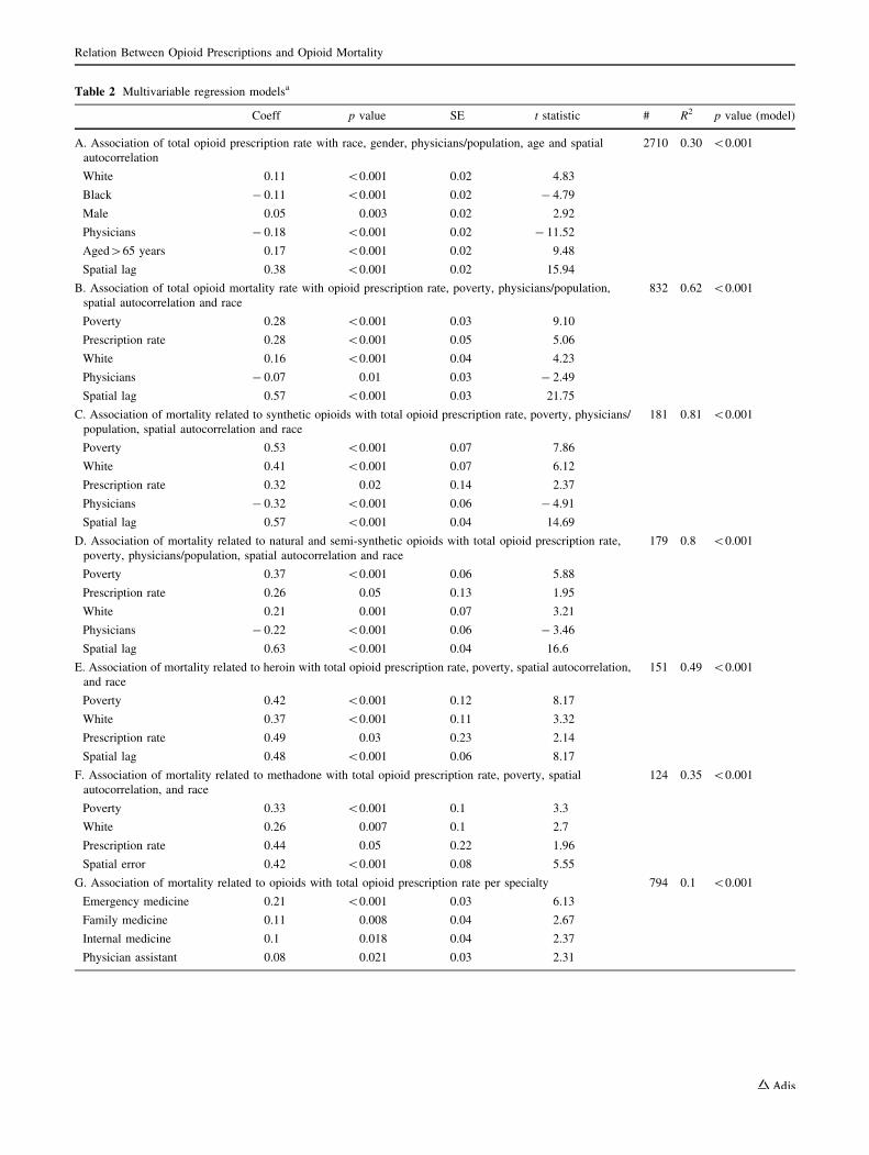
Table 2 Multivariable regression modelsa
Coeff p value SE t statistic # R2 p value (model)
A. Association of total opioid prescription rate with race, gender, physicians/population, age and spatial
autocorrelation
2710 0.30 \0.001
White 0.11 \0.001 0.02 4.83
Black - 0.11 \0.001 0.02 - 4.79
Male 0.05 0.003 0.02 2.92
Physicians - 0.18 \0.001 0.02 - 11.52
Aged[65 years 0.17 \0.001 0.02 9.48
Spatial lag 0.38 \0.001 0.02 15.94
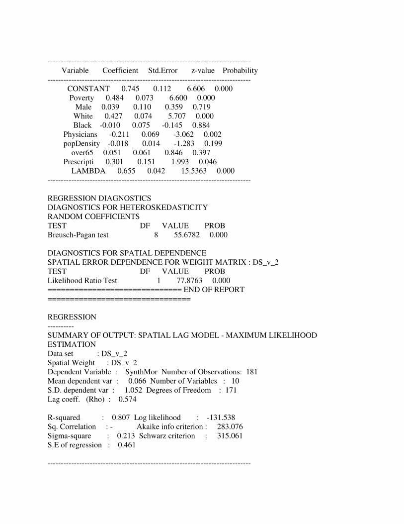
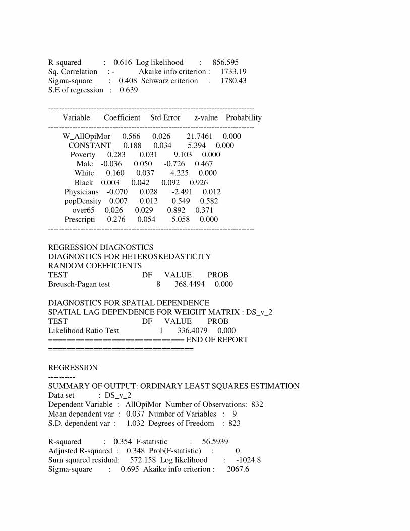
B. Association of total opioid mortality rate with opioid prescription rate, poverty, physicians/population,
spatial autocorrelation and race
832 0.62 \0.001
Poverty 0.28 \0.001 0.03 9.10
Prescription rate 0.28 \0.001 0.05 5.06
White 0.16 \0.001 0.04 4.23
Physicians - 0.07 0.01 0.03 - 2.49
Spatial lag 0.57 \0.001 0.03 21.75
C. Association of mortality related to synthetic opioids with total opioid prescription rate, poverty, physicians/
population, spatial autocorrelation and race
181 0.81 \0.001
Poverty 0.53 \0.001 0.07 7.86
White 0.41 \0.001 0.07 6.12
Prescription rate 0.32 0.02 0.14 2.37
Physicians - 0.32 \0.001 0.06 - 4.91
Spatial lag 0.57 \0.001 0.04 14.69
D. Association of mortality related to natural and semi-synthetic opioids with total opioid prescription rate,
poverty, physicians/population, spatial autocorrelation and race
179 0.8 \0.001
Poverty 0.37 \0.001 0.06 5.88
Prescription rate 0.26 0.05 0.13 1.95
White 0.21 0.001 0.07 3.21
Physicians - 0.22 \0.001 0.06 - 3.46
Spatial lag 0.63 \0.001 0.04 16.6
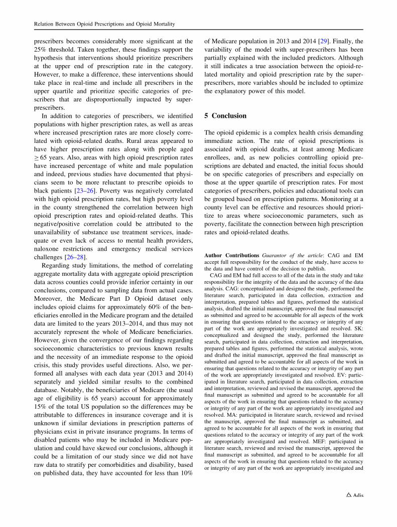
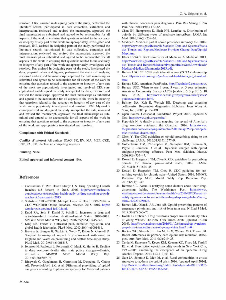
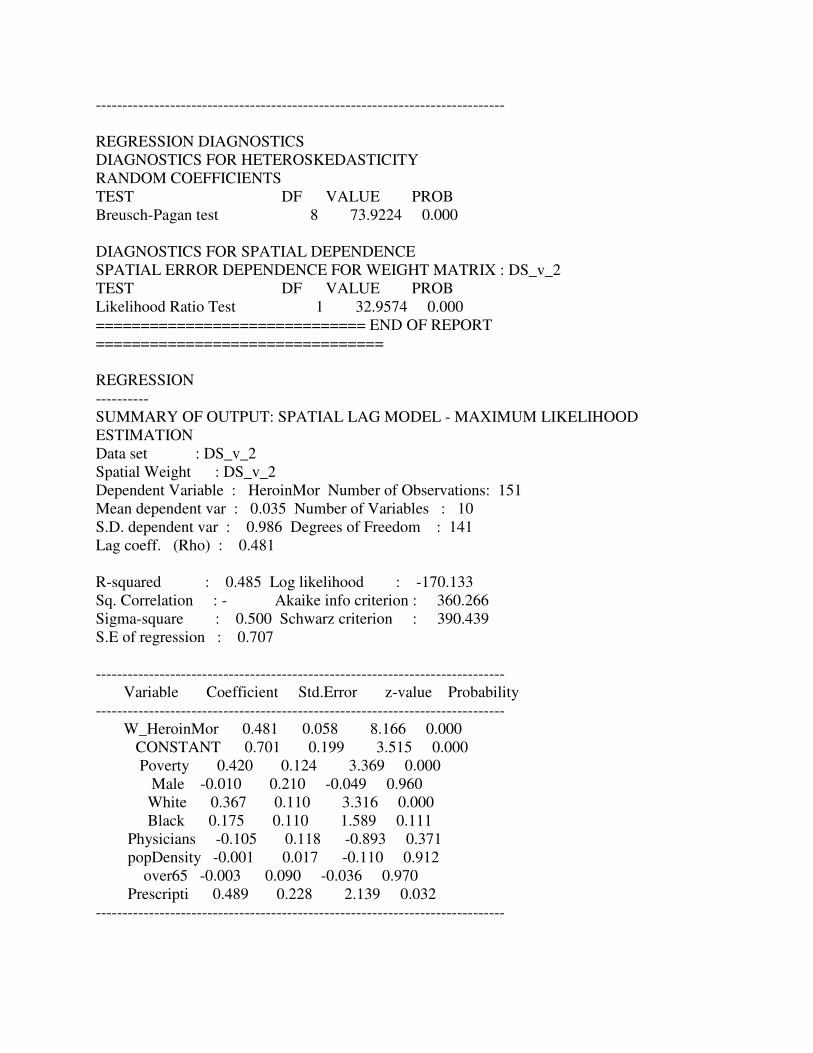
E. Association of mortality related to heroin with total opioid prescription rate, poverty, spatial autocorrelation,
and race
151 0.49 \0.001
Poverty 0.42 \0.001 0.12 8.17
White 0.37 \0.001 0.11 3.32
Prescription rate 0.49 0.03 0.23 2.14
Spatial lag 0.48 \0.001 0.06 8.17
F. Association of mortality related to methadone with total opioid prescription rate, poverty, spatial
autocorrelation, and race
124 0.35 \0.001
Poverty 0.33 \0.001 0.1 3.3
White 0.26 0.007 0.1 2.7
Prescription rate 0.44 0.05 0.22 1.96
Spatial error 0.42 \0.001 0.08 5.55
G. Association of mortality related to opioids with total opioid prescription rate per specialty 794 0.1 \0.001
Emergency medicine 0.21 \0.001 0.03 6.13
Family medicine 0.11 0.008 0.04 2.67
Internal medicine 0.1 0.018 0.04 2.37
Physician assistant 0.08 0.021 0.03 2.31
Relation Between Opioid Prescriptions and Opioid Mortality
linearly associated with the total opioid prescription rate and
35% of the variance of total opioid-related mortality was
correlated with opioid prescription rate (pmodel\0.001,
R2 = 0.35) (Table 2B). This correlation between opioid
prescription rate, poverty, % of white population and opioid
mortality was consistent with each opioid mortality category
[natural/semi-synthetic opioids (pmodel\0.001, R2 = 0.45)
(Table 2D), synthetic opioids (pmodel\0.001, R2 = 0.52)
(Table 2C), heroin (pmodel\0.001, R2 = 0.18) (Table 2E)
and methadone (pmodel\0.001, R2 = 0.35)] (Table 2F).
The correlation with poverty is particularly interesting,
especially since poverty was negatively correlated with the
opioid prescription rate. To further examine this correlation,
we compared the fitted single linear regression lines of the
total opioid mortality to the prescription rate in counties
above and below the median poverty level and found that
the impact of prescription rate in opioid mortality in
counties with high poverty (p\0.001, Coeff = 0.51) was
higher than in counties with lower poverty (p\0.001,
Coeff = 0.35). This finding indicates that, even though
poverty is negatively correlated with the opioid prescription
rate in areas with high poverty, high prescription rate is
closely correlated with high opioid-related mortality.
Then, we analyzed data on the prescription patterns
among 93 categories of prescribers and found that 10 cat-
egories accounted for 90.22% of all opioid claims.
Breaking down the opioid prescription per category, family
medicine practitioners ranked first, accounting for 31.15%
of all opioid claims reported, prescribing 5.32 opioid
claims per beneficiary who received an opioid prescription.
Internal medicine physicians prescribed 29.04% of all
opioid claims reported, with 5.11 opioid claims per bene-
ficiary, while nurse practitioners and physician assistants
were accountable for 6.64% of all opioid claims, pre-
scribing 3.81 and 2.74 opioid claims per beneficiary who
received an opioid prescription, respectively (Table 3A,
eFig. 1, and eTable 2). Because the top 10 medical cate-
gories accounted for 9 out of 10 of all opioid claims, we
fitted a multivariable linear regression model to examine
the impact of the opioid prescription rate of these cate-
gories in opioid-related mortality at a county level and we
found that overall opioid prescription rates provided by
emergency medicine, family medicine physicians, internal
medicine and physician assistants were positively associ-
ated with opioid-related mortality (Table 2A).
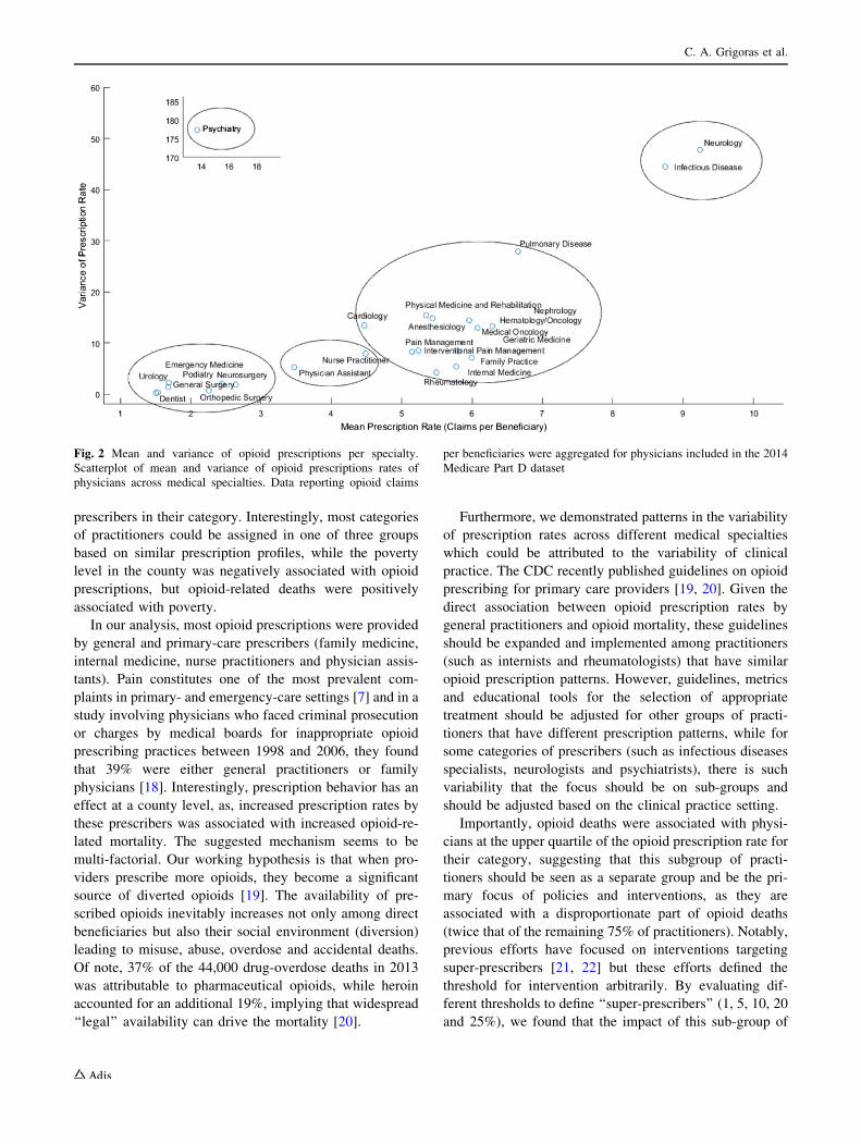
We included the top 25 opioid-prescribing medical spe-
cialties accounting for more than 98% of all opioid pre-
scriptions and estimated the mean and the variance of the
prescription rate of physicians for each medical specialty
and displayed them graphically (Fig. 2). Based on the dis-
tribution of the prescription rates, we identified five groups
of medical specialties with similar combinations of mean
prescription rates and variances, providing potential groups
of practitioners who, on average, have similar opioid pre-
scription patterns. The first category consisted mostly of
surgical specialties and emergency-medicine physicians,
while the second included advanced practice providers
(nurse practitioners and physician assistants). The third
group included mostly internal and family-medicine prac-
titioners and oncologists. Interestingly, in the last two
groups, that were considerably smaller with respect to the
number of specialties, we observed both higher variance and
mean prescription rates. More specifically, the fourth group
consisted of neurologists and infectious diseases practi-
tioners. This difference from the previous groups could be
attributed to the variability of clinical practice among the
specialists in the same field which reflects the patients’
characteristics. Even higher variability was detected in the
fifth category, which included the psychiatrists. These
findings indicate that regarding opioid policies, educational
tools and metrics, one size does not ‘‘fit all’’ and, while some
prescribers could be grouped, others should be highly dif-
ferentiated based on practice characteristics.
Interestingly, we found that a minority of prescribers
contributed most prescriptions, and that was particularly
characteristic of specific categories of practitioners. For
example, the top 25% of physician assistants prescribed
more than 55% of the opioids prescribed in this category,
while in other categories that are more closely associated
with the use of opioid agents (such as hematologists/on-
cologists) the contribution of these prescribers was more
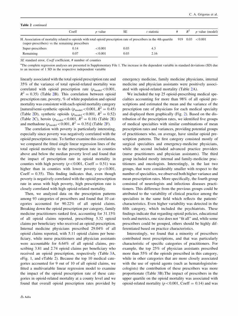
proportionate (Table 3B).The impact of prescribers in the
upper quartile on the opioid mortality was associated with
opioid-related mortality (p\0.001, Coeff = 0.14) and was
Table 2 continued
Coeff p value SE t statistic # R2 p value (model)
H. Association of mortality related to opioids with total opioid prescription rate of prescribers in the 4th quartile
(super-prescribers) vs the remaining prescribers
919 0.03 \0.001
Super-prescribers 0.14 \0.001 0.03 4.3
Remaining 0.07 \0.001 0.03 2.16
SE standard error, Coeff coefficient, # number of countiesaThe complete regression analyses are presented in Supplementary File 1. The increase in the dependent variable in standard deviations (SD) due
to an increase of 1 SD in the respective independent variable
C. A. Grigoras et al.

twice that of the remaining 75% of practitioners (p\0.001,
Coeff = 0.07) (pmodel = 0.03, R2 = 0.03) (Table 3B).
4 Discussion
The USA faces an opioid overdose epidemic [16, 17].
Using the Medicare Part D nationwide database, we found
that opioid prescription rates varied widely, and at a county
level, the opioid prescription rate was associated with
opioid-related mortality (in total, as well as for each cate-
gory of opioids and heroin). Most opioid prescriptions were
provided in the primary/general-care setting and were
related to the percent of white and male population in the
county. Moreover, opioid-related deaths were correlated
with the opioid prescription rate of specific categories of
practitioners and they were disproportionally associated
with prescribers who belonged to the upper quartile of
Table 3 Opioid prescription rate per medical specialty
A.
Specialty # of counties Opioid beneficiaries Opioid claims Claims per beneficiary Proportion of total
opioid claims (%)
Family practice 2826 10,549,952 56,158,035 5.32 31.15
Internal medicine 2238 10,237,738 52,354,379 5.11 29.04
Nurse practitioner 2418 3,146,818 11,976,790 3.81 6.64
Physician assistant 1954 3,333,374 9,136,242 2.74 5.07
Orthopedic surgery 1423 3,951,371 9,023,800 2.28 5.01
Interventional pain management 474 1,234,933 5,747,668 4.65 3.19
Anesthesiology 582 1,215,039 5,730,458 4.72 3.18
Emergency medicine 1814 3,847,040 5,132,330 1.33 2.85
Rheumatology 626 785,773 3,957,165 5.04 2.19
Pain management 399 723,269 3,435,111 4.75 1.91
General surgery 1659 1,333,230 2,052,799 1.54 1.14
Neurology 632 345,828 2,034,899 5.88 1.13
Dentist 2011 1,264,041 1,668,344 1.32 0.93
Hematology/oncology 708 286,779 1,436,653 5.01 0.8
Geriatric medicine 309 239,845 1,310,961 5.47 0.73
Urology 979 653,803 960,123 1.47 0.53
Neurosurgery 490 366,319 956,279 2.61 0.53
Oral surgery (dentists only) 754 676,883 814,350 1.2 0.45
Cardiology 448 160,787 622,956 3.87 0.35
Podiatry 934 276,597 605,814 2.19 0.34
B.
Specialty Proportion of total prescriptions
due to physicians in the
upper quartile (%)
Proportion of total prescriptions
due to physicians in the
lower quartile (%)
Mean of prescription
rate (claims/beneficiary)
Standard deviation
of prescription rate
Physician assistant 55.58 8.03 1.67 0.85
Cardiology 50.00 6.49 2.77 1.42
Nurse practitioner 48.03 5.31 2.79 1.50
Emergency medicine 42.27 8.53 0.99 0.01
Internal medicine 40.23 5.26 3.61 1.53
Family practice 38.56 7.71 3.88 1.47
Anesthesiology 38.52 10.03 3.73 1.34
Geriatric medicine 37.28 12.07 3.80 1.12
Pain management 35.76 13.59 3.88 1.22
Podiatry 35.19 12.69 1.68 0.45
The list contains the top 20 prescribing medical specialties, accountable for 97.16% of all opioid prescriptions. Combined data from Medicare
Part D datasets for 2013 and 2014
Relation Between Opioid Prescriptions and Opioid Mortality
prescribers in their category. Interestingly, most categories
of practitioners could be assigned in one of three groups
based on similar prescription profiles, while the poverty
level in the county was negatively associated with opioid
prescriptions, but opioid-related deaths were positively
associated with poverty.
In our analysis, most opioid prescriptions were provided
by general and primary-care prescribers (family medicine,
internal medicine, nurse practitioners and physician assis-
tants). Pain constitutes one of the most prevalent com-
plaints in primary- and emergency-care settings [7] and in a
study involving physicians who faced criminal prosecution
or charges by medical boards for inappropriate opioid
prescribing practices between 1998 and 2006, they found
that 39% were either general practitioners or family
physicians [18]. Interestingly, prescription behavior has an
effect at a county level, as, increased prescription rates by
these prescribers was associated with increased opioid-re-
lated mortality. The suggested mechanism seems to be
multi-factorial. Our working hypothesis is that when pro-
viders prescribe more opioids, they become a significant
source of diverted opioids [19]. The availability of pre-
scribed opioids inevitably increases not only among direct
beneficiaries but also their social environment (diversion)
leading to misuse, abuse, overdose and accidental deaths.
Of note, 37% of the 44,000 drug-overdose deaths in 2013
was attributable to pharmaceutical opioids, while heroin
accounted for an additional 19%, implying that widespread
‘‘legal’’ availability can drive the mortality [20].
Furthermore, we demonstrated patterns in the variability
of prescription rates across different medical specialties
which could be attributed to the variability of clinical
practice. The CDC recently published guidelines on opioid
prescribing for primary care providers [19, 20]. Given the
direct association between opioid prescription rates by
general practitioners and opioid mortality, these guidelines
should be expanded and implemented among practitioners
(such as internists and rheumatologists) that have similar
opioid prescription patterns. However, guidelines, metrics
and educational tools for the selection of appropriate
treatment should be adjusted for other groups of practi-
tioners that have different prescription patterns, while for
some categories of prescribers (such as infectious diseases
specialists, neurologists and psychiatrists), there is such
variability that the focus should be on sub-groups and
should be adjusted based on the clinical practice setting.
Importantly, opioid deaths were associated with physi-
cians at the upper quartile of the opioid prescription rate for
their category, suggesting that this subgroup of practi-
tioners should be seen as a separate group and be the pri-
mary focus of policies and interventions, as they are
associated with a disproportionate part of opioid deaths
(twice that of the remaining 75% of practitioners). Notably,
previous efforts have focused on interventions targeting
super-prescribers [21, 22] but these efforts defined the
threshold for intervention arbitrarily. By evaluating dif-
ferent thresholds to define ‘‘super-prescribers’’ (1, 5, 10, 20
and 25%), we found that the impact of this sub-group of
Fig. 2 Mean and variance of opioid prescriptions per specialty.
Scatterplot of mean and variance of opioid prescriptions rates of
physicians across medical specialties. Data reporting opioid claims
per beneficiaries were aggregated for physicians included in the 2014
Medicare Part D dataset
C. A. Grigoras et al.
prescribers becomes considerably more significant at the
25% threshold. Taken together, these findings support the
hypothesis that interventions should prioritize prescribers
at the upper end of prescription rate in the category.
However, to make a difference, these interventions should
take place in real-time and include all prescribers in the
upper quartile and prioritize specific categories of pre-
scribers that are disproportionally impacted by super-
prescribers.
In addition to categories of prescribers, we identified
populations with higher prescription rates, as well as areas
where increased prescription rates are more closely corre-
lated with opioid-related deaths. Rural areas appeared to
have higher prescription rates along with people aged
C 65 years. Also, areas with high opioid prescription rates
have increased percentage of white and male population
and indeed, previous studies have documented that physi-
cians seem to be more reluctant to prescribe opioids to
black patients [23–26]. Poverty was negatively correlated
with high opioid prescription rates, but high poverty level
in the county strengthened the correlation between high
opioid prescription rates and opioid-related deaths. This
negative/positive correlation could be attributed to the
unavailability of substance use treatment services, inade-
quate or even lack of access to mental health providers,
naloxone restrictions and emergency medical services
challenges [26–28].
Regarding study limitations, the method of correlating
aggregate mortality data with aggregate opioid prescription
data across counties could provide inferior certainty in our
conclusions, compared to sampling data from actual cases.
Moreover, the Medicare Part D Opioid dataset only
includes opioid claims for approximately 60% of the ben-
eficiaries enrolled in the Medicare program and the detailed
data are limited to the years 2013–2014, and thus may not
accurately represent the whole of Medicare beneficiaries.
However, given the convergence of our findings regarding
socioeconomic characteristics to previous known results
and the necessity of an immediate response to the opioid
crisis, this study provides useful directions. Also, we per-
formed all analyses with each data year (2013 and 2014)
separately and yielded similar results to the combined
database. Notably, the beneficiaries of Medicare (the usual
age of eligibility is 65 years) account for approximately
15% of the total US population so the differences may be
attributable to differences in insurance coverage and it is
unknown if similar deviations in prescription patterns of
physicians exist in private insurance programs. In terms of
disabled patients who may be included in Medicare pop-
ulation and could have skewed our conclusions, although it
could be a limitation of our study since we did not have
raw data to stratify per comorbidities and disability, based
on published data, they have accounted for less than 10%
of Medicare population in 2013 and 2014 [29]. Finally, the
variability of the model with super-prescribers has been
partially explained with the included predictors. Although
it still indicates a true association between the opioid-re-
lated mortality and opioid prescription rate by the super-
prescribers, more variables should be included to optimize
the explanatory power of this model.
5 Conclusion
The opioid epidemic is a complex health crisis demanding
immediate action. The rate of opioid prescriptions is
associated with opioid deaths, at least among Medicare
enrollees, and, as new policies controlling opioid pre-
scriptions are debated and enacted, the initial focus should
be on specific categories of prescribers and especially on
those at the upper quartile of prescription rates. For most
categories of prescribers, policies and educational tools can
be grouped based on prescription patterns. Monitoring at a
county level can be effective and resources should priori-
tize to areas where socioeconomic parameters, such as
poverty, facilitate the connection between high prescription
rates and opioid-related deaths.
Author Contributions Guarantor of the article: CAG and EM
accept full responsibility for the conduct of the study, have access to
the data and have control of the decision to publish.
CAG and EM had full access to all of the data in the study and take
responsibility for the integrity of the data and the accuracy of the data
analysis. CAG: conceptualized and designed the study, performed the
literature search, participated in data collection, extraction and
interpretation, prepared tables and figures, performed the statistical
analysis, drafted the initial manuscript, approved the final manuscript
as submitted and agreed to be accountable for all aspects of the work
in ensuring that questions related to the accuracy or integrity of any
part of the work are appropriately investigated and resolved. SK:
conceptualized and designed the study, performed the literature
search, participated in data collection, extraction and interpretation,
prepared tables and figures, performed the statistical analysis, wrote
and drafted the initial manuscript, approved the final manuscript as
submitted and agreed to be accountable for all aspects of the work in
ensuring that questions related to the accuracy or integrity of any part
of the work are appropriately investigated and resolved. EV: partic-
ipated in literature search, participated in data collection, extraction
and interpretation, reviewed and revised the manuscript, approved the
final manuscript as submitted and agreed to be accountable for all
aspects of the work in ensuring that questions related to the accuracy
or integrity of any part of the work are appropriately investigated and
resolved. MA: participated in literature search, reviewed and revised
the manuscript, approved the final manuscript as submitted, and
agreed to be accountable for all aspects of the work in ensuring that
questions related to the accuracy or integrity of any part of the work
are appropriately investigated and resolved. MEF: participated in
literature search, reviewed and revised the manuscript, approved the
final manuscript as submitted, and agreed to be accountable for all
aspects of the work in ensuring that questions related to the accuracy
or integrity of any part of the work are appropriately investigated and
Relation Between Opioid Prescriptions and Opioid Mortality
resolved. CKR: assisted in designing parts of the study, performed the
literature search, participated in data collection, extraction and
interpretation, reviewed and revised the manuscript, approved the
final manuscript as submitted and agreed to be accountable for all
aspects of the work in ensuring that questions related to the accuracy
or integrity of any part of the work are appropriately investigated and
resolved. INE: assisted in designing parts of the study, performed the
literature search, participated in data collection, extraction and
interpretation, reviewed and revised the manuscript, approved the
final manuscript as submitted and agreed to be accountable for all
aspects of the work in ensuring that questions related to the accuracy
or integrity of any part of the work are appropriately investigated and
resolved. PA: assisted in designing parts of the study, interpreted the
data, prepared tables and figures, performed the statistical analysis,
reviewed and revised the manuscript, approved the final manuscript as
submitted and agreed to be accountable for all aspects of the work in
ensuring that questions related to the accuracy or integrity of any part
of the work are appropriately investigated and resolved. CIS: con-
ceptualized and designed the study, interpreted the data, reviewed and
revised the manuscript, approved the final manuscript as submitted
and agreed to be accountable for all aspects of the work in ensuring
that questions related to the accuracy or integrity of any part of the
work are appropriately investigated and resolved. EM: Mylonakis
conceptualized and designed the study, interpreted the data, reviewed
and revised the manuscript, approved the final manuscript as sub-
mitted and agreed to be accountable for all aspects of the work in
ensuring that questions related to the accuracy or integrity of any part
of the work are appropriately investigated and resolved.
Compliance with Ethical Standards
Conflict of interest All authors [CAG, SK, EV, MA, MEF, CKR,
INE, PA, EM] declare no competing interests
Funding None.
Ethical approval and informed consent N/A.
References
1. Constantino T. IMS Health Study: U.S. Drug Spending Growth
Reaches 8.5 Percent in 2015. 2016. http://www.imshealth.
com/en/about-us/news/ims-health-study-us-drug-spending-growth-
reaches-8.5-percent-in-2015.
2. Statistics CfDCaPNCfH. Multiple Cause of Death 1999–2014 on
CDC WONDER Online Database, released 2015. 2016. http://
wonder.cdc.gov/mcd-icd10.html.
3. Rudd RA, Seth P, David F, Scholl L. Increases in drug and
opioid-involved overdose deaths—United States, 2010–2015.
MMWR Morb Mortal Wkly Rep. 2016;65(5051):1445–52.
4. King NB, Fraser V. Untreated pain, narcotics regulation, and
global health ideologies. PLoS Med. 2013;10(4):e1001411.
5. Hawton K, Bergen H, Simkin S, Wells C, Kapur N, Gunnell D.
Six-year follow-up of impact of co-proxamol withdrawal in
England and Wales on prescribing and deaths: time-series study.
PLoS Med. 2012;9(5):e1001213.
6. Johnson H, Paulozzi L, Porucznik C, Mack K, Herter B. Decline
in drug overdose deaths after state policy changes—Florida,
2010–2012. MMWR Morb Mortal Wkly Rep.
2014;63(26):569–74.
7. Ringwalt C, Gugelmann H, Garrettson M, Dasgupta N, Chung
AE, Proescholdbell SK, et al. Differential prescribing of opioid
analgesics according to physician specialty for Medicaid patients
with chronic noncancer pain diagnoses. Pain Res Manag J Can
Pain Soc. 2014;19(4):179–85.
8. Chen JH, Humphreys K, Shah NH, Lembke A. Distribution of
opioids by different types of medicare prescribers. JAMA Int
Med. 2016;176(2):259–61.
9. Medicare. Medicare part D opioid prescriber summary file. 2016.
https://www.cms.gov/Research-Statistics-Data-and-Systems/Statis
tics-Trends-and-Reports/Medicare-Provider-Charge-Data/Opioid
Map.html.
10. Klees BSWCJ. Brief summaries of Medicare & Medicaid 2013.
https://www.cms.gov/Research-Statistics-Data-and-Systems/Statis
tics-Trends-and-Reports/MedicareProgramRatesStats/Downloads/
MedicareMedicaidSummaries2013.pdf.
11. Bureau USC. 2010 ZIP code tabulation area (ZCTA) relationship
files. https://www.census.gov/geo/maps-data/data/zcta_rel_download.
html.
12. Bureau USC. American FactFinder. http://factfinder2.census.gov/.
13. Bureau USC. When to use 1-year, 3-year, or 5-year estimates
American Community Survey (ACS) [updated 6 Sep 2016, 18
July 2016]. http://www.census.gov/programs-surveys/acs/
guidance/estimates.html.
14. Belsley DA, Kuh E, Welsch RE. Detecting and assessing
collinearity. Regression diagnostics. Hoboken: John Wiley &
Sons, Inc.; 2005. p. 85–191.
15. Open Source Geospatial Foundation Project 2016. Updated 5
Nov. http://www.qgis.org/en/site/.
16. Popovich N. A deadly crisis: mapping the spread of America’s
drug overdose epidemic: the Guardian. 2016. https://www.
theguardian.com/society/ng-interactive/2016/may/25/opioid-epide
mic-overdose-deaths-map.
17. Olsen Y. The CDC guideline on opioid prescribing: rising to the
challenge. JAMA. 2016;315(15):1577–9.
18. Goldenbaum DM, Christopher M, Gallagher RM, Fishman S,
Payne R, Joranson D, et al. Physicians charged with opioid
analgesic-prescribing offenses. Pain Med (Malden, Mass.).
2008;9(6):737–47.
19. Dowell D, Haegerich TM, Chou R. CDc guideline for prescribing
opioids for chronic pain—united states, 2016. JAMA.
2016;315(15):1624–45.
20. Dowell D, Haegerich TM, Chou R. CDC guideline for pre-
scribing opioids for chronic pain—United States, 2016. MMWR
Recomm Rep Morb Mortal Wkly Rep Recomm Rep.
2016;65(1):1–49.
21. Bernstein L. Aetna is notifying some doctors about their drug-
dispensing habits. The Washington Post. https://www.
washingtonpost.com/news/to-your-health/wp/2016/08/03/aetna-is-
notifying-some-doctors-about-their-drug-dispensing-habits/?utm_
term=.52929125f028.
22. Barnett ML, Olenski AR, Jena AB. Opioid-prescribing patterns of
emergency physicians and risk of long-term use. N Engl J Med.
2017;376(7):663–73.
23. Kolata G, Cohen S. Drug overdoses proper rise in mortality rates
of young Whites. The New York Times. 2016. [updated 16 Jan
2016]. http://www.nytimes.com/2016/01/17/science/drug-overdoses-
propel-rise-in-mortality-rates-of-young-whites.html?_r=0.
24. Becker WC, Starrels JL, Heo M, Li X, Weiner MG, Turner BJ.
Racial differences in primary care opioid risk reduction strate-
gies. Ann Fam Med. 2011;9(3):219–25.
25. Cerda M, Ransome Y, Keyes KM, Koenen KC, Tracy M, Tardiff
KJ, et al. Prescription opioid mortality trends in New York City,
1990–2006: examining the emergence of an epidemic. Drug
Alcohol Depend. 2013;132(1–2):53–62.
26. Gale JA, Schmitz D, Meit M, et al. Rural communities in crisis:
strategies to address the opioid crisis 2016. [updated April 2016].http://www.ruralhealthweb.org/index.cfm?objectid=DB1783C2-
DB37-0073-AE5A339A5336A09E.
C. A. Grigoras et al.

27. Mack KA, Zhang K, Paulozzi L, Jones C. Prescription practices
involving opioid analgesics among Americans with Medicaid,
2010. J Health Care Poor Underserved. 2015;26(1):182–98.
28. CDC. Opioid painkiller prescribing 2016 [updated 1 July 2014].
http://www.cdc.gov/vitalsigns/opioid-prescribing/.
29. SERVICES USDOHAH. 2014 CMS statistics 2014. https://www.
cms.gov/Research-Statistics-Data-and-Systems/Statistics-Trends-
and-Reports/CMS-Statistics-Reference-Booklet/Downloads/CMS_
Stats_2014_final.pdf.
Relation Between Opioid Prescriptions and Opioid Mortality

Supplementary Material
Sensitivity Analysis of opioid mortality association with prescription rates of super-prescribers
Physicians identified as “super-prescribers” if they belonged in the 75th
percentile of prescription
rates and “remaining” otherwise.
Estimate
SE
tStat
pValue
(Intercept) -1.820e-16 0.032 -5.598e-15 0.999
Remaining 0.071 0.033 2.162 0.030
Super-Prescribers 0.143 0.033 4.301 1.877e-05
Number of observations: 919, Error degrees of freedom: 916, Root Mean Squared Error: 0.99, R-
squared: 0.03, Adjusted R-Squared: 0.03, F-statistic vs. constant model: 14.17, p-value = 0.
Physicians identified as super-prescribers if they belonged in the 80th
percentile of prescription
rates
Estimate
SE
tStat
pValue
(Intercept) 1.733e-15 0.032 5.283e-14 0.999
Remaining 0.068 0.033 2.037 0.041
Super-Prescribers 0.137 0.033 4.069 5.119e-05
Number of observations: 905, Error degrees of freedom: 902, Root Mean Squared Error: 0.99, R-
squared: 0.03, Adjusted R-Squared: 0.03, F-statistic vs. constant model: 12.83, p-value = 0.
Physicians identified as super-prescribers if they belonged in the 90th
percentile of prescription
rates

Estimate
SE
tStat
pValue
(Intercept) 7.028e-16 0.033 2.116e-14 0.999
Remaining 0.081 0.033 2.429 0.015
Super-Prescribers 0.139 0.033 4.169 3.352e-05
Number of observations: 882, Error degrees of freedom: 879, Root Mean Squared Error: 0.99, R-
squared: 0.03, Adjusted R-Squared: 0.03, F-statistic vs. constant model: 13.23, p-value = 0.
Physicians identified as super-prescribers if they belonged in the 95th
percentile of prescription
rates
Estimate
SE
tStat
pValue
(Intercept) 3.965e-16 0.034 1.154e-14 0.999
Remaining 0.121 0.034 3.517 0.000
Super-Prescribers 0.103 0.034 3.000 0.002
Number of observations: 826, Error degrees of freedom: 823, Root Mean Squared Error: 0.99, R-
squared: 0.03, Adjusted R-Squared: 0.02, F-statistic vs. constant model: 11.57, p-value = 0.
Physicians identified as super-prescribers if they belonged in the 99th
percentile of prescription
rates
Estimate
SE
tStat
pValue
(Intercept) -1.060e-15 0.041 -2.526e-14 0.999
Remaining 0.231 0.042 5.498 5.975e-08
Super-Prescribers 0.139 0.042 3.322 0.000

Number of observations: 528, Error degrees of freedom: 525, Root Mean Squared Error: 0.96, R-
squared: 0.07, Adjusted R-Squared: 0.07, F-statistic vs. constant model: 20.83, p-value = 0.
Spatial Regression Analyses
REGRESSION
----------
SUMMARY OF OUTPUT: SPATIAL ERROR MODEL - MAXIMUM LIKELIHOOD
ESTIMATION
Data set : DS_v_2
Spatial Weight : DS_v_2
Dependent Variable : Methadone Number of Observations: 124
Mean dependent var : -0.177 Number of Variables : 9
S.D. dependent var : 0.691 Degrees of Freedom : 115
Lag coeff. (Lambda) : 0.427
R-squared : 0.389 R-squared (BUSE) : -
Sq. Correlation : - Log likelihood : -104.454
Sigma-square : 0.292 Akaike info criterion : 226.908
S.E of regression : 0.540 Schwarz criterion : 252.291
-----------------------------------------------------------------------------
Variable Coefficient Std.Error z-value Probability
-----------------------------------------------------------------------------
CONSTANT 0.668 0.192 3.471 0.000
Poverty 0.329 0.100 3.297 0.000
Male 0.291 0.191 1.518 0.128
White 0.258 0.095 2.7027 0.006
Black 0.074 0.093 0.802 0.422
Physicians -0.030 0.101 -0.300 0.763
popDensity 0.005 0.015 0.351 0.725
over65 0.145 0.084 1.726 0.084
Prescripti 0.435 0.221 1.967 0.049
LAMBDA 0.427 0.077 5.548 0.000
-----------------------------------------------------------------------------
REGRESSION DIAGNOSTICS
DIAGNOSTICS FOR HETEROSKEDASTICITY
RANDOM COEFFICIENTS
TEST DF VALUE PROB
Breusch-Pagan test 8 108.5154 0.000

DIAGNOSTICS FOR SPATIAL DEPENDENCE
SPATIAL ERROR DEPENDENCE FOR WEIGHT MATRIX : DS_v_2
TEST DF VALUE PROB
Likelihood Ratio Test 1 22.1881 0.000
============================== END OF REPORT
================================
REGRESSION
----------
SUMMARY OF OUTPUT: SPATIAL LAG MODEL - MAXIMUM LIKELIHOOD
ESTIMATION
Data set : DS_v_2
Spatial Weight : DS_v_2
Dependent Variable : Methadone Number of Observations: 124
Mean dependent var : -0.177 Number of Variables : 10
S.D. dependent var : 0.691 Degrees of Freedom : 114
Lag coeff. (Rho) : 0.349
R-squared : 0.348 Log likelihood : -106.708
Sq. Correlation : - Akaike info criterion : 233.416
Sigma-square : 0.311 Schwarz criterion : 261.619
S.E of regression : 0.557
-----------------------------------------------------------------------------
Variable Coefficient Std.Error z-value Probability
-----------------------------------------------------------------------------
W_Methadone 0.349 0.078 4.473 0.000
CONSTANT 0.639 0.186 3.433 0.000
Poverty 0.261 0.109 2.391 0.016
Male 0.273 0.194 1.409 0.158
White 0.229 0.099 2.301 0.021
Black 0.139 0.092 1.495 0.134
Physicians -0.058 0.106 -0.553 0.580
popDensity 0.008 0.014 0.609 0.542
over65 0.179 0.078 2.2883 0.022
Prescripti 0.387 0.217 1.782 0.074
-----------------------------------------------------------------------------
REGRESSION DIAGNOSTICS
DIAGNOSTICS FOR HETEROSKEDASTICITY
RANDOM COEFFICIENTS
TEST DF VALUE PROB
Breusch-Pagan test 8 101.4547 0.000
DIAGNOSTICS FOR SPATIAL DEPENDENCE

SPATIAL LAG DEPENDENCE FOR WEIGHT MATRIX : DS_v_2
TEST DF VALUE PROB
Likelihood Ratio Test 1 17.6808 0.000
============================== END OF REPORT
================================
REGRESSION
----------
SUMMARY OF OUTPUT: ORDINARY LEAST SQUARES ESTIMATION
Data set : DS_v_2
Dependent Variable : Methadone Number of Observations: 124
Mean dependent var : -0.177 Number of Variables : 9
S.D. dependent var : 0.691 Degrees of Freedom : 115
R-squared : 0.210 F-statistic : 3.832
Adjusted R-squared : 0.155 Prob(F-statistic) : 0.000
Sum squared residual: 46.8095 Log likelihood : -115.548
Sigma-square : 0.407 Akaike info criterion : 249.097
S.E. of regression : 0.637 Schwarz criterion : 274.479
Sigma-square ML : 0.377
S.E of regression ML: 0.614
-----------------------------------------------------------------------------
Variable Coefficient Std.Error t-Statistic Probability
-----------------------------------------------------------------------------
CONSTANT 0.631 0.212 2.974 0.003
Poverty 0.231 0.124 1.856 0.065
Male 0.341 0.221 1.538 0.126
White 0.228 0.113 2.007 0.047
Black 0.170 0.106 1.608 0.110
Physicians 0.035 0.121 0.289 0.772
popDensity 0.009 0.016 0.563 0.574
over65 0.230 0.089 2.571 0.011
Prescripti 0.407 0.247 1.644 0.102
-----------------------------------------------------------------------------
REGRESSION DIAGNOSTICS
MULTICOLLINEARITY CONDITION NUMBER 9.672
TEST ON NORMALITY OF ERRORS
TEST DF VALUE PROB
Jarque-Bera 2 263.8651 0.000
DIAGNOSTICS FOR HETEROSKEDASTICITY
RANDOM COEFFICIENTS
TEST DF VALUE PROB
Breusch-Pagan test 8 95.6224 0.000

Koenker-Bassett test 8 23.7926 0.002
DIAGNOSTICS FOR SPATIAL DEPENDENCE
FOR WEIGHT MATRIX : DS_v_2
(row-standardized weights)
TEST MI/DF VALUE PROB
Moran's I (error) 0.3673 4.7648 0.000
Lagrange Multiplier (lag) 1 18.5596 0.000
Robust LM (lag) 1 0.0683 0.793
Lagrange Multiplier (error) 1 19.9929 0.000
Robust LM (error) 1 1.5016 0.220
Lagrange Multiplier (SARMA) 2 20.0612 0.000
============================== END OF REPORT
================================
REGRESSION
----------
SUMMARY OF OUTPUT: SPATIAL ERROR MODEL - MAXIMUM LIKELIHOOD
ESTIMATION
Data set : DS_v_2
Spatial Weight : DS_v_2
Dependent Variable : HeroinMor Number of Observations: 151
Mean dependent var : 0.035 Number of Variables : 9
S.D. dependent var : 0.986 Degrees of Freedom : 142
Lag coeff. (Lambda) : 0.488
R-squared : 0.463 R-squared (BUSE) : -
Sq. Correlation : - Log likelihood : -173.617
Sigma-square : 0.522 Akaike info criterion : 365.234
S.E of regression : 0.722 Schwarz criterion : 392.39
-----------------------------------------------------------------------------
Variable Coefficient Std.Error z-value Probability
-----------------------------------------------------------------------------
CONSTANT 0.547 0.206 2.651 0.008
Poverty 0.390 0.123 3.162 0.001
Male -0.002 0.218 -0.010 0.991
White 0.380 0.117 3.235 0.001
Black 0.108 0.118 0.910 0.362
Physicians -0.005 0.117 -0.043 0.965
popDensity -0.007 0.020 -0.339 0.734
over65 -0.028 0.102 -0.276 0.782
Prescripti 0.337 0.243 1.387 0.165
LAMBDA 0.488 0.062 7.800 0.000
-----------------------------------------------------------------------------
REGRESSION DIAGNOSTICS
DIAGNOSTICS FOR HETEROSKEDASTICITY
RANDOM COEFFICIENTS
TEST DF VALUE PROB
Breusch-Pagan test 8 73.9224 0.000
DIAGNOSTICS FOR SPATIAL DEPENDENCE
SPATIAL ERROR DEPENDENCE FOR WEIGHT MATRIX : DS_v_2
TEST DF VALUE PROB
Likelihood Ratio Test 1 32.9574 0.000
============================== END OF REPORT
================================
REGRESSION
----------
SUMMARY OF OUTPUT: SPATIAL LAG MODEL - MAXIMUM LIKELIHOOD
ESTIMATION
Data set : DS_v_2
Spatial Weight : DS_v_2
Dependent Variable : HeroinMor Number of Observations: 151
Mean dependent var : 0.035 Number of Variables : 10
S.D. dependent var : 0.986 Degrees of Freedom : 141
Lag coeff. (Rho) : 0.481
R-squared : 0.485 Log likelihood : -170.133
Sq. Correlation : - Akaike info criterion : 360.266
Sigma-square : 0.500 Schwarz criterion : 390.439
S.E of regression : 0.707
-----------------------------------------------------------------------------
Variable Coefficient Std.Error z-value Probability
-----------------------------------------------------------------------------
W_HeroinMor 0.481 0.058 8.166 0.000
CONSTANT 0.701 0.199 3.515 0.000
Poverty 0.420 0.124 3.369 0.000
Male -0.010 0.210 -0.049 0.960
White 0.367 0.110 3.316 0.000
Black 0.175 0.110 1.589 0.111
Physicians -0.105 0.118 -0.893 0.371
popDensity -0.001 0.017 -0.110 0.912
over65 -0.003 0.090 -0.036 0.970
Prescripti 0.489 0.228 2.139 0.032
-----------------------------------------------------------------------------
REGRESSION DIAGNOSTICS
DIAGNOSTICS FOR HETEROSKEDASTICITY
RANDOM COEFFICIENTS
TEST DF VALUE PROB
Breusch-Pagan test 8 78.6754 0.000
DIAGNOSTICS FOR SPATIAL DEPENDENCE
SPATIAL LAG DEPENDENCE FOR WEIGHT MATRIX : DS_v_2
TEST DF VALUE PROB
Likelihood Ratio Test 1 39.9257 0.000
============================== END OF REPORT
================================
REGRESSION
----------
SUMMARY OF OUTPUT: ORDINARY LEAST SQUARES ESTIMATION
Data set : DS_v_2
Dependent Variable : HeroinMor Number of Observations: 151
Mean dependent var : 0.035 Number of Variables : 9
S.D. dependent var : 0.986 Degrees of Freedom : 142
R-squared : 0.253 F-statistic : 6.017
Adjusted R-squared : 0.211 Prob(F-statistic) :1.187e-006
Sum squared residual: 109.643 Log likelihood : -190.096
Sigma-square : 0.772 Akaike info criterion : 398.192
S.E. of regression : 0.878 Schwarz criterion : 425.347
Sigma-square ML : 0.726
S.E of regression ML: 0.852
-----------------------------------------------------------------------------
Variable Coefficient Std.Error t-Statistic Probability
-----------------------------------------------------------------------------
CONSTANT 0.819 0.247 3.316 0.001
Poverty 0.545 0.154 3.536 0.000
Male -0.095 0.260 -0.364 0.715
White 0.594 0.135 4.373 0.000
Black 0.209 0.137 1.528 0.128
Physicians -0.186 0.146 -1.270 0.206
popDensity -0.009 0.022 -0.416 0.677
over65 -0.051 0.112 -0.457 0.648
Prescripti 0.451 0.283 1.590 0.114
-----------------------------------------------------------------------------
REGRESSION DIAGNOSTICS
MULTICOLLINEARITY CONDITION NUMBER 9.038
TEST ON NORMALITY OF ERRORS

TEST DF VALUE PROB
Jarque-Bera 2 159.9630 0.000
DIAGNOSTICS FOR HETEROSKEDASTICITY
RANDOM COEFFICIENTS
TEST DF VALUE PROB
Breusch-Pagan test 8 42.4868 0.000
Koenker-Bassett test 8 14.0637 0.080
DIAGNOSTICS FOR SPATIAL DEPENDENCE
FOR WEIGHT MATRIX : DS_v_2
(row-standardized weights)
TEST MI/DF VALUE PROB
Moran's I (error) 0.3874 5.3280 0.000
Lagrange Multiplier (lag) 1 32.9800 0.000
Robust LM (lag) 1 8.4345 0.003
Lagrange Multiplier (error) 1 25.4930 0.000
Robust LM (error) 1 0.9475 0.330
Lagrange Multiplier (SARMA) 2 33.9276 0.000
============================== END OF REPORT
================================
REGRESSION
----------
SUMMARY OF OUTPUT: SPATIAL ERROR MODEL - MAXIMUM LIKELIHOOD
ESTIMATION
Data set : DS_v_2
Spatial Weight : DS_v_2
Dependent Variable : OtherOpMo Number of Observations: 179
Mean dependent var : -0.119 Number of Variables : 9
S.D. dependent var : 1.007 Degrees of Freedom : 170
Lag coeff. (Lambda) : 0.700
R-squared : 0.782 R-squared (BUSE) : -
Sq. Correlation : - Log likelihood : -143.249
Sigma-square : 0.220 Akaike info criterion : 304.5
S.E of regression : 0.469 Schwarz criterion : 333.186
-----------------------------------------------------------------------------
Variable Coefficient Std.Error z-value Probability
-----------------------------------------------------------------------------
CONSTANT 0.264 0.110 2.390 0.016
Poverty 0.287 0.070 4.091 0.000
Male 0.042 0.114 0.368 0.712

White 0.206 0.072 2.869 0.004
Black -0.046 0.072 -0.637 0.523
Physicians -0.086 0.066 -1.298 0.194
popDensity -0.013 0.014 -0.953 0.340
over65 0.031 0.059 0.528 0.597
Prescripti 0.209 0.144 1.443 0.148
LAMBDA 0.700 0.037 18.7312 0.000
-----------------------------------------------------------------------------
REGRESSION DIAGNOSTICS
DIAGNOSTICS FOR HETEROSKEDASTICITY
RANDOM COEFFICIENTS
TEST DF VALUE PROB
Breusch-Pagan test 8 100.5837 0.000
DIAGNOSTICS FOR SPATIAL DEPENDENCE
SPATIAL ERROR DEPENDENCE FOR WEIGHT MATRIX : DS_v_2
TEST DF VALUE PROB
Likelihood Ratio Test 1 118.2458 0.000
============================== END OF REPORT
================================
REGRESSION
----------
SUMMARY OF OUTPUT: SPATIAL LAG MODEL - MAXIMUM LIKELIHOOD
ESTIMATION
Data set : DS_v_2
Spatial Weight : DS_v_2
Dependent Variable : OtherOpMo Number of Observations: 179
Mean dependent var : -0.119 Number of Variables : 10
S.D. dependent var : 1.007 Degrees of Freedom : 169
Lag coeff. (Rho) : 0.638
R-squared : 0.800 Log likelihood : -130.098
Sq. Correlation : - Akaike info criterion : 280.197
Sigma-square : 0.202 Schwarz criterion : 312.07
S.E of regression : 0.449
-----------------------------------------------------------------------------
Variable Coefficient Std.Error z-value Probability
-----------------------------------------------------------------------------
W_OtherOpMo 0.638 0.038 16.6045 0.000
CONSTANT 0.486 0.096 5.045 0.000
Poverty 0.379 0.064 5.882 0.000
Male 0.025 0.110 0.232 0.816
White 0.209 0.065 3.205 0.001

Black -0.028 0.066 -0.431 0.665
Physicians -0.219 0.063 -3.462 0.000
popDensity -0.011 0.011 -1.029 0.303
over65 0.055 0.048 1.155 0.247
Prescripti 0.258 0.132 1.946 0.051
-----------------------------------------------------------------------------
REGRESSION DIAGNOSTICS
DIAGNOSTICS FOR HETEROSKEDASTICITY
RANDOM COEFFICIENTS
TEST DF VALUE PROB
Breusch-Pagan test 8 79.7611 0.000
DIAGNOSTICS FOR SPATIAL DEPENDENCE
SPATIAL LAG DEPENDENCE FOR WEIGHT MATRIX : DS_v_2
TEST DF VALUE PROB
Likelihood Ratio Test 1 144.5490 0.000
============================== END OF REPORT
================================
REGRESSION
----------
SUMMARY OF OUTPUT: ORDINARY LEAST SQUARES ESTIMATION
Data set : DS_v_2
Dependent Variable : OtherOpMo Number of Observations: 179
Mean dependent var : -0.119 Number of Variables : 9
S.D. dependent var : 1.007 Degrees of Freedom : 170
R-squared : 0.446 F-statistic : 17.1419
Adjusted R-squared : 0.420 Prob(F-statistic) :1.492e-018
Sum squared residual: 100.55 Log likelihood : -202.373
Sigma-square : 0.591 Akaike info criterion : 422.746
S.E. of regression : 0.769 Schwarz criterion : 451.432
Sigma-square ML : 0.561
S.E of regression ML: 0.749
-----------------------------------------------------------------------------
Variable Coefficient Std.Error t-Statistic Probability
-----------------------------------------------------------------------------
CONSTANT 0.977 0.162 6.008 0.000
Poverty 0.835 0.106 7.878 0.000
Male -0.005 0.187 -0.026 0.978
White 0.337 0.110 3.044 0.002
Black -0.154 0.112 -1.371 0.171
Physicians -0.319 0.108 -2.951 0.003
popDensity -0.031 0.018 -1.696 0.091

over65 0.094 0.082 1.150 0.251
Prescripti 0.589 0.225 2.611 0.009
-----------------------------------------------------------------------------
REGRESSION DIAGNOSTICS
MULTICOLLINEARITY CONDITION NUMBER 8.209
TEST ON NORMALITY OF ERRORS
TEST DF VALUE PROB
Jarque-Bera 2 3704.5592 0.000
DIAGNOSTICS FOR HETEROSKEDASTICITY
RANDOM COEFFICIENTS
TEST DF VALUE PROB
Breusch-Pagan test 8 72.8554 0.000
Koenker-Bassett test 8 6.2825 0.615
DIAGNOSTICS FOR SPATIAL DEPENDENCE
FOR WEIGHT MATRIX : DS_v_2
(row-standardized weights)
TEST MI/DF VALUE PROB
Moran's I (error) 0.5609 8.2952 0.000
Lagrange Multiplier (lag) 1 107.7762 0.000
Robust LM (lag) 1 47.3559 0.000
Lagrange Multiplier (error) 1 63.9086 0.000
Robust LM (error) 1 3.4883 0.061
Lagrange Multiplier (SARMA) 2 111.2645 0.000
============================== END OF REPORT
================================
REGRESSION
----------
SUMMARY OF OUTPUT: SPATIAL ERROR MODEL - MAXIMUM LIKELIHOOD
ESTIMATION
Data set : DS_v_2
Spatial Weight : DS_v_2
Dependent Variable : SynthMor Number of Observations: 181
Mean dependent var : 0.066 Number of Variables : 9
S.D. dependent var : 1.052 Degrees of Freedom : 172
Lag coeff. (Lambda) : 0.655
R-squared : 0.782 R-squared (BUSE) : -
Sq. Correlation : - Log likelihood : -148.581
Sigma-square : 0.2413 Akaike info criterion : 315.163
S.E of regression : 0.491 Schwarz criterion : 343.95
-----------------------------------------------------------------------------
Variable Coefficient Std.Error z-value Probability
-----------------------------------------------------------------------------
CONSTANT 0.745 0.112 6.606 0.000
Poverty 0.484 0.073 6.600 0.000
Male 0.039 0.110 0.359 0.719
White 0.427 0.074 5.707 0.000
Black -0.010 0.075 -0.145 0.884
Physicians -0.211 0.069 -3.062 0.002
popDensity -0.018 0.014 -1.283 0.199
over65 0.051 0.061 0.846 0.397
Prescripti 0.301 0.151 1.993 0.046
LAMBDA 0.655 0.042 15.5363 0.000
-----------------------------------------------------------------------------
REGRESSION DIAGNOSTICS
DIAGNOSTICS FOR HETEROSKEDASTICITY
RANDOM COEFFICIENTS
TEST DF VALUE PROB
Breusch-Pagan test 8 55.6782 0.000
DIAGNOSTICS FOR SPATIAL DEPENDENCE
SPATIAL ERROR DEPENDENCE FOR WEIGHT MATRIX : DS_v_2
TEST DF VALUE PROB
Likelihood Ratio Test 1 77.8763 0.000
============================== END OF REPORT
================================
REGRESSION
----------
SUMMARY OF OUTPUT: SPATIAL LAG MODEL - MAXIMUM LIKELIHOOD
ESTIMATION
Data set : DS_v_2
Spatial Weight : DS_v_2
Dependent Variable : SynthMor Number of Observations: 181
Mean dependent var : 0.066 Number of Variables : 10
S.D. dependent var : 1.052 Degrees of Freedom : 171
Lag coeff. (Rho) : 0.574
R-squared : 0.807 Log likelihood : -131.538
Sq. Correlation : - Akaike info criterion : 283.076
Sigma-square : 0.213 Schwarz criterion : 315.061
S.E of regression : 0.461
-----------------------------------------------------------------------------

Variable Coefficient Std.Error z-value Probability
-----------------------------------------------------------------------------
W_SynthMor 0.574 0.039 14.6933 0.000
CONSTANT 0.847 0.097 8.649 0.000
Poverty 0.526 0.067 7.855 0.000
Male 0.095 0.103 0.923 0.355
White 0.413 0.067 6.119 0.000
Black 0.041 0.067 0.617 0.537
Physicians -0.317 0.064 -4.900 0.000
popDensity -0.012 0.011 -1.104 0.269
over65 0.081 0.048 1.6712 0.094
Prescripti 0.323 0.136 2.369 0.017
-----------------------------------------------------------------------------
REGRESSION DIAGNOSTICS
DIAGNOSTICS FOR HETEROSKEDASTICITY
RANDOM COEFFICIENTS
TEST DF VALUE PROB
Breusch-Pagan test 8 29.5392 0.000
DIAGNOSTICS FOR SPATIAL DEPENDENCE
SPATIAL LAG DEPENDENCE FOR WEIGHT MATRIX : DS_v_2
TEST DF VALUE PROB
Likelihood Ratio Test 1 111.9642 0.000
============================== END OF REPORT
================================
REGRESSION
----------
SUMMARY OF OUTPUT: ORDINARY LEAST SQUARES ESTIMATION
Data set : DS_v_2
Dependent Variable : SynthMor Number of Observations: 181
Mean dependent var : 0.066 Number of Variables : 9
S.D. dependent var : 1.052 Degrees of Freedom : 172
R-squared : 0.580 F-statistic : 29.743
Adjusted R-squared : 0.560 Prob(F-statistic) :8.289e-029
Sum squared residual: 84.1552 Log likelihood : -187.52
Sigma-square : 0.489 Akaike info criterion : 393.04
S.E. of regression : 0.699 Schwarz criterion : 421.826
Sigma-square ML : 0.464
S.E of regression ML: 0.681
-----------------------------------------------------------------------------
Variable Coefficient Std.Error t-Statistic Probability
-----------------------------------------------------------------------------

CONSTANT 1.287 0.142 9.007 0.000
Poverty 0.907 0.096 9.4173 0.000
Male -0.087 0.155 -0.564 0.572
White 0.616 0.100 6.145 0.000
Black -0.040 0.100 -0.397 0.691
Physicians -0.425 0.098 -4.340 0.000
popDensity -0.034 0.016 -2.045 0.042
over65 0.097 0.074 1.3201 0.188
Prescripti 0.591 0.205 2.8823 0.004
-----------------------------------------------------------------------------
REGRESSION DIAGNOSTICS
MULTICOLLINEARITY CONDITION NUMBER 8.102
TEST ON NORMALITY OF ERRORS
TEST DF VALUE PROB
Jarque-Bera 2 974.7218 0.000
DIAGNOSTICS FOR HETEROSKEDASTICITY
RANDOM COEFFICIENTS
TEST DF VALUE PROB
Breusch-Pagan test 8 70.4228 0.000
Koenker-Bassett test 8 11.2336 0.188
DIAGNOSTICS FOR SPATIAL DEPENDENCE
FOR WEIGHT MATRIX : DS_v_2
(row-standardized weights)
TEST MI/DF VALUE PROB
Moran's I (error) 0.4572 6.8760 0.000
Lagrange Multiplier (lag) 1 81.4796 0.000
Robust LM (lag) 1 39.0484 0.000
Lagrange Multiplier (error) 1 43.4210 0.000
Robust LM (error) 1 0.9898 0.319
Lagrange Multiplier (SARMA) 2 82.4694 0.000
============================== END OF REPORT
================================
REGRESSION
----------
SUMMARY OF OUTPUT: SPATIAL ERROR MODEL - MAXIMUM LIKELIHOOD
ESTIMATION
Data set : DS_v_2
Spatial Weight : DS_v_2
Dependent Variable : AllOpiMor Number of Observations: 832
Mean dependent var : 0.037 Number of Variables : 9

S.D. dependent var : 1.032 Degrees of Freedom : 823
Lag coeff. (Lambda) : 0.617
R-squared : 0.614 R-squared (BUSE) : -
Sq. Correlation : - Log likelihood : -870.182
Sigma-square : 0.410 Akaike info criterion : 1758.36
S.E of regression : 0.640 Schwarz criterion : 1800.88
-----------------------------------------------------------------------------
Variable Coefficient Std.Error z-value Probability
-----------------------------------------------------------------------------
CONSTANT 0.088 0.057 1.546 0.121
Poverty 0.339 0.037 9.006 0.000
Male -0.002 0.050 -0.050 0.959
White 0.227 0.053 4.261 0.000
Black -0.049 0.055 -0.880 0.378
Physicians -0.008 0.028 -0.292 0.769
popDensity 0.001 0.017 0.101 0.919
over65 0.041 0.035 1.159 0.246
Prescripti 0.277 0.059 4.646 0.000
LAMBDA 0.617 0.025 23.89 0.000
-----------------------------------------------------------------------------
REGRESSION DIAGNOSTICS
DIAGNOSTICS FOR HETEROSKEDASTICITY
RANDOM COEFFICIENTS
TEST DF VALUE PROB
Breusch-Pagan test 8 411.4742 0.000
DIAGNOSTICS FOR SPATIAL DEPENDENCE
SPATIAL ERROR DEPENDENCE FOR WEIGHT MATRIX : DS_v_2
TEST DF VALUE PROB
Likelihood Ratio Test 1 309.2338 0.000
============================== END OF REPORT
================================
REGRESSION
----------
SUMMARY OF OUTPUT: SPATIAL LAG MODEL - MAXIMUM LIKELIHOOD
ESTIMATION
Data set : DS_v_2
Spatial Weight : DS_v_2
Dependent Variable : AllOpiMor Number of Observations: 832
Mean dependent var : 0.037 Number of Variables : 10
S.D. dependent var : 1.032 Degrees of Freedom : 822
Lag coeff. (Rho) : 0.566
R-squared : 0.616 Log likelihood : -856.595
Sq. Correlation : - Akaike info criterion : 1733.19
Sigma-square : 0.408 Schwarz criterion : 1780.43
S.E of regression : 0.639
-----------------------------------------------------------------------------
Variable Coefficient Std.Error z-value Probability
-----------------------------------------------------------------------------
W_AllOpiMor 0.566 0.026 21.7461 0.000
CONSTANT 0.188 0.034 5.394 0.000
Poverty 0.283 0.031 9.103 0.000
Male -0.036 0.050 -0.726 0.467
White 0.160 0.037 4.225 0.000
Black 0.003 0.042 0.092 0.926
Physicians -0.070 0.028 -2.491 0.012
popDensity 0.007 0.012 0.549 0.582
over65 0.026 0.029 0.892 0.371
Prescripti 0.276 0.054 5.058 0.000
-----------------------------------------------------------------------------
REGRESSION DIAGNOSTICS
DIAGNOSTICS FOR HETEROSKEDASTICITY
RANDOM COEFFICIENTS
TEST DF VALUE PROB
Breusch-Pagan test 8 368.4494 0.000
DIAGNOSTICS FOR SPATIAL DEPENDENCE
SPATIAL LAG DEPENDENCE FOR WEIGHT MATRIX : DS_v_2
TEST DF VALUE PROB
Likelihood Ratio Test 1 336.4079 0.000
============================== END OF REPORT
================================
REGRESSION
----------
SUMMARY OF OUTPUT: ORDINARY LEAST SQUARES ESTIMATION
Data set : DS_v_2
Dependent Variable : AllOpiMor Number of Observations: 832
Mean dependent var : 0.037 Number of Variables : 9
S.D. dependent var : 1.032 Degrees of Freedom : 823
R-squared : 0.354 F-statistic : 56.5939
Adjusted R-squared : 0.348 Prob(F-statistic) : 0
Sum squared residual: 572.158 Log likelihood : -1024.8
Sigma-square : 0.695 Akaike info criterion : 2067.6

S.E. of regression : 0.833 Schwarz criterion : 2110.11
Sigma-square ML : 0.687
S.E of regression ML: 0.829
-----------------------------------------------------------------------------
Variable Coefficient Std.Error t-Statistic Probability
-----------------------------------------------------------------------------
CONSTANT 0.326 0.045 7.192 0.000
Poverty 0.542 0.038 14.0568 0.000
Male -0.120 0.066 -1.820 0.068
White 0.272 0.048 5.620 0.000
Black -0.083 0.054 -1.519 0.129
Physicians -0.068 0.036 -1.856 0.063
popDensity -0.000 0.016 -0.015 0.987
over65 -0.006 0.037 -0.182 0.854
Prescripti 0.484 0.070 6.834 0.000
-----------------------------------------------------------------------------
REGRESSION DIAGNOSTICS
MULTICOLLINEARITY CONDITION NUMBER 3.737
TEST ON NORMALITY OF ERRORS
TEST DF VALUE PROB
Jarque-Bera 2 15062.8995 0.000
DIAGNOSTICS FOR HETEROSKEDASTICITY
RANDOM COEFFICIENTS
TEST DF VALUE PROB
Breusch-Pagan test 8 280.6823 0.000
Koenker-Bassett test 8 25.6147 0.001
DIAGNOSTICS FOR SPATIAL DEPENDENCE
FOR WEIGHT MATRIX : DS_v_2
(row-standardized weights)
TEST MI/DF VALUE PROB
Moran's I (error) 0.4756 17.3304 0.000
Lagrange Multiplier (lag) 1 342.4862 0.000
Robust LM (lag) 1 51.8084 0.000
Lagrange Multiplier (error) 1 291.3827 0.000
Robust LM (error) 1 0.7049 0.401
Lagrange Multiplier (SARMA) 2 343.1911 0.000
============================== END OF REPORT
================================
REGRESSION

----------
SUMMARY OF OUTPUT: SPATIAL ERROR MODEL - MAXIMUM LIKELIHOOD
ESTIMATION
Data set : DS_v_2
Spatial Weight : DS_v_2
Dependent Variable : Prescripti Number of Observations: 2710
Mean dependent var : 0.008 Number of Variables : 8
S.D. dependent var : 0.986 Degrees of Freedom : 2702
Lag coeff. (Lambda) : 0.398
R-squared : 0.298 R-squared (BUSE) : -
Sq. Correlation : - Log likelihood :-3370.126
Sigma-square : 0.682 Akaike info criterion : 6756.25
S.E of regression : 0.825 Schwarz criterion : 6803.49
-----------------------------------------------------------------------------
Variable Coefficient Std.Error z-value Probability
-----------------------------------------------------------------------------
CONSTANT 0.003 0.026 0.143 0.885
Poverty 0.034 0.024 1.407 0.159
Male 0.049 0.017 2.795 0.005
White 0.118 0.032 3.600 0.000
Black -0.175 0.031 -5.525 0.000
Physicians -0.182 0.015 -11.4965 0.000
popDensity -0.015 0.019 -0.807 0.419
over65 0.186 0.020 9.010 0.000
LAMBDA 0.398 0.025 15.6241 0.000
-----------------------------------------------------------------------------
REGRESSION DIAGNOSTICS
DIAGNOSTICS FOR HETEROSKEDASTICITY
RANDOM COEFFICIENTS
TEST DF VALUE PROB
Breusch-Pagan test 7 331.8550 0.000
DIAGNOSTICS FOR SPATIAL DEPENDENCE
SPATIAL ERROR DEPENDENCE FOR WEIGHT MATRIX : DS_v_2
TEST DF VALUE PROB
Likelihood Ratio Test 1 218.2767 0.000
============================== END OF REPORT
================================
REGRESSION
----------
SUMMARY OF OUTPUT: SPATIAL LAG MODEL - MAXIMUM LIKELIHOOD
ESTIMATION
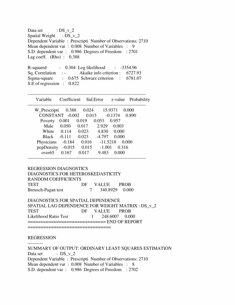
Data set : DS_v_2
Spatial Weight : DS_v_2
Dependent Variable : Prescripti Number of Observations: 2710
Mean dependent var : 0.008 Number of Variables : 9
S.D. dependent var : 0.986 Degrees of Freedom : 2701
Lag coeff. (Rho) : 0.388
R-squared : 0.304 Log likelihood : -3354.96
Sq. Correlation : - Akaike info criterion : 6727.93
Sigma-square : 0.675 Schwarz criterion : 6781.07
S.E of regression : 0.822
-----------------------------------------------------------------------------
Variable Coefficient Std.Error z-value Probability
-----------------------------------------------------------------------------
W_Prescripti 0.388 0.024 15.9371 0.000
CONSTANT -0.002 0.015 -0.1374 0.890
Poverty 0.001 0.019 0.053 0.957
Male 0.050 0.017 2.929 0.003
White 0.114 0.023 4.830 0.000
Black -0.111 0.023 -4.797 0.000
Physicians -0.184 0.016 -11.5218 0.000
popDensity -0.015 0.015 -1.001 0.316
over65 0.167 0.017 9.483 0.000
-----------------------------------------------------------------------------
REGRESSION DIAGNOSTICS
DIAGNOSTICS FOR HETEROSKEDASTICITY
RANDOM COEFFICIENTS
TEST DF VALUE PROB
Breusch-Pagan test 7 340.8929 0.000
DIAGNOSTICS FOR SPATIAL DEPENDENCE
SPATIAL LAG DEPENDENCE FOR WEIGHT MATRIX : DS_v_2
TEST DF VALUE PROB
Likelihood Ratio Test 1 248.6007 0.000
============================== END OF REPORT
================================
REGRESSION
----------
SUMMARY OF OUTPUT: ORDINARY LEAST SQUARES ESTIMATION
Data set : DS_v_2
Dependent Variable : Prescripti Number of Observations: 2710
Mean dependent var : 0.008 Number of Variables : 8
S.D. dependent var : 0.986 Degrees of Freedom : 2702
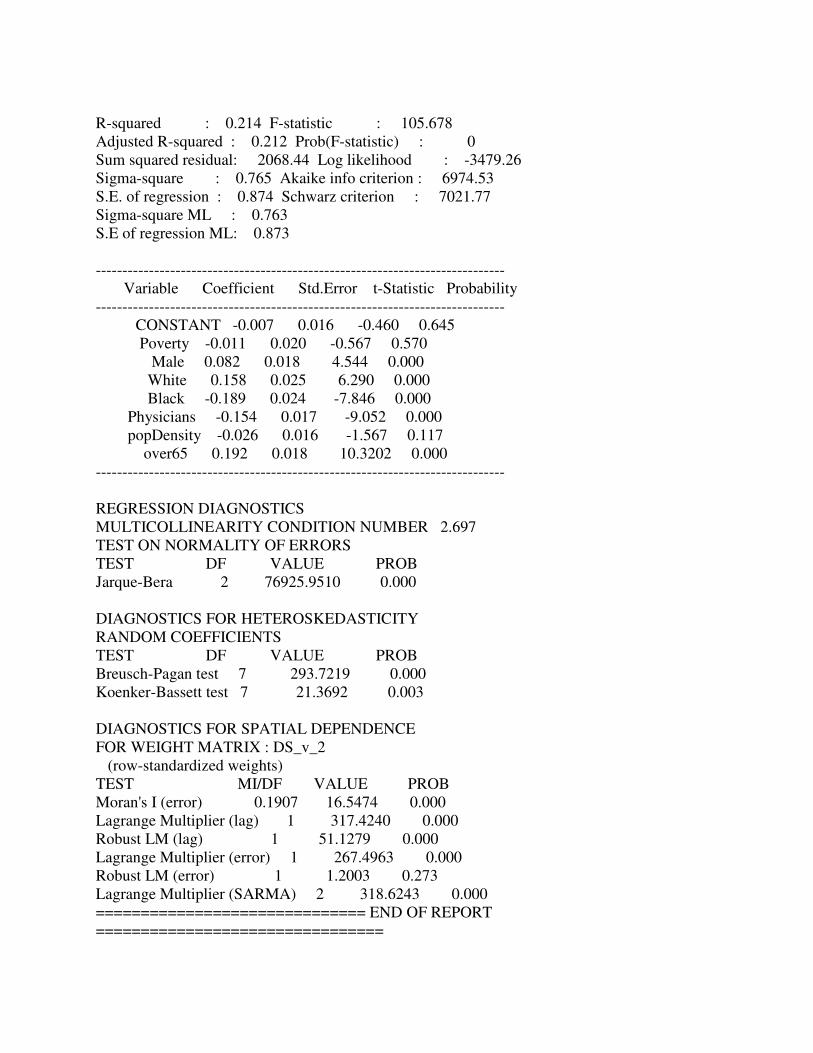
R-squared : 0.214 F-statistic : 105.678
Adjusted R-squared : 0.212 Prob(F-statistic) : 0
Sum squared residual: 2068.44 Log likelihood : -3479.26
Sigma-square : 0.765 Akaike info criterion : 6974.53
S.E. of regression : 0.874 Schwarz criterion : 7021.77
Sigma-square ML : 0.763
S.E of regression ML: 0.873
-----------------------------------------------------------------------------
Variable Coefficient Std.Error t-Statistic Probability
-----------------------------------------------------------------------------
CONSTANT -0.007 0.016 -0.460 0.645
Poverty -0.011 0.020 -0.567 0.570
Male 0.082 0.018 4.544 0.000
White 0.158 0.025 6.290 0.000
Black -0.189 0.024 -7.846 0.000
Physicians -0.154 0.017 -9.052 0.000
popDensity -0.026 0.016 -1.567 0.117
over65 0.192 0.018 10.3202 0.000
-----------------------------------------------------------------------------
REGRESSION DIAGNOSTICS
MULTICOLLINEARITY CONDITION NUMBER 2.697
TEST ON NORMALITY OF ERRORS
TEST DF VALUE PROB
Jarque-Bera 2 76925.9510 0.000
DIAGNOSTICS FOR HETEROSKEDASTICITY
RANDOM COEFFICIENTS
TEST DF VALUE PROB
Breusch-Pagan test 7 293.7219 0.000
Koenker-Bassett test 7 21.3692 0.003
DIAGNOSTICS FOR SPATIAL DEPENDENCE
FOR WEIGHT MATRIX : DS_v_2
(row-standardized weights)
TEST MI/DF VALUE PROB
Moran's I (error) 0.1907 16.5474 0.000
Lagrange Multiplier (lag) 1 317.4240 0.000
Robust LM (lag) 1 51.1279 0.000
Lagrange Multiplier (error) 1 267.4963 0.000
Robust LM (error) 1 1.2003 0.273
Lagrange Multiplier (SARMA) 2 318.6243 0.000
============================== END OF REPORT
================================