Correlation

Correlation is a statistical technique that is used to measure and describe the relationship between two variables.

Usually the two variables are simply observed as they exist naturally in the environment—there is no attempt to

control or manipulate the variables.

The Characteristics of a Relationship

A correlation is a numerical value that describes and measures three characteristics of the relationship between X

and Y. These three characteristics are as follows:

1. The Direction of the Relationship. The sign of the correlation, positive or negative, describes the

direction of the relationship.

D e f i n i t i o n s:

In a positive correlation, the two variables tend to change in the same direction: As the value of the X

variable increases from one individual to another, the Y variable also tends to increase; when the X

variable decreases, the Y variable also decreases.

In a negative correlation, the two variables tend to go in opposite directions. As the X variable increases,

the Y variable decreases. That is, it is an inverse relationship.

2. The Form of the Relationship. In the preceding coffee and beer examples, the relationships tend to

have a linear form; that is, the points in the scatter plot tend to cluster around a straight line. We have

drawn a line through the middle of the data points in each figure to help show the relationship. The most

common use of correlation is to measure straight-line relationships. However, other forms of

relationships do exist and there are special correlations used to measure them.

3. The Strength or Consistency of the Relationship. Finally, the correlation measures the consistency

of the relationship. For a linear relationship, for example, the data points could fit perfectly on a straight

line. Every time X increases by one point, the value of Y also changes by a consistent and predictable

amount. Figure 14.3(a) shows an example of a perfect linear relationship. However, relationships are

usually not perfect. Although there may be a tendency for the value of Y to increase whenever X

increases, the amount that Y changes is not always the same, and occasionally, Y decreases when X

increases. In this situation, the data points do not fall perfectly on a straight line. The consistency of the

relationship is measured by the numerical value of the correlation. A perfect correlation always is

identified by a correlation of 1.00 and indicates a perfectly consistent relationship. For a correlation of

1.00 (or –1.00), each change in X is accompanied by a perfectly predictable change in Y. At the other

extreme, a correlation of 0 indicates no consistency at all. For a correlation of 0, the data points are

scattered randomly with no clear trend [see Figure 14.3(b)]. Intermediate values between 0 and 1 indicate

the degree of consistency.

There are three different kinds of correlation that will be discussed in the following order

1- Pearson’s r

2- Spearman’s ρ

3- Pearson’s ϕ

4- The Point-Biserial Correlation

1. The Pearson Correlation

By far the most common correlation is the Pearson correlation (or the Pearson product–moment correlation)

which measures the degree of straight-line relationship.

D e f i n i t i o n

The Pearson correlation measures the degree and the direction of the linearrelationship between two variables.

The Pearson correlation is identified by the letter r. Conceptually, this correlation is computed by

When there is a perfect linear relationship, every change in the X variable is accompanied by a corresponding

change in the Y variable.

EXAMPLE:

The Pearson Correlation and z-Scores

The Pearson correlation measures the relationship between an individual’s location in the X distribution and his

or her location in the Y distribution. For example, a positive correlation means that individuals who have a high

X score also tend to have a high Y score. Similarly, a negative correlation indicates that individuals with high X

scores tend to have low Y scores.

z-scores identify the exact location of each individual score within a distribution. With this in mind, each X value

can be transformed into a z-score, zX, using the mean and standard deviation for the set of Xs. Similarly, each Y

score can be transformed into zY. If the X and Y values are viewed as a sample, then the transformation is

completed using the sample formula for z . If the X and Y values form a complete population, then the z-scores

are computed . After the transformation, the formula for the Pearson correlation can be expressed entirely in

terms of z-scores

Using and Interpreting the Pearson Correlation

Where and Why Correlations Are Used

1. Prediction. If two variables are known to be related in a systematic way, then it is possible to use one of the

variables to make predictions about the other.

2. Validity. Suppose that a psychologist develops a new test for measuring intelligence. How could you show

that this test truly measures what it claims; that is, how could you demonstrate the validity of the test? One

common technique for demonstrating validity is to use a correlation. If the test actually measures intelligence,

then the scores on the test should be related to other measures of intelligence—for example, standardized IQ

tests, performance on learning tasks, problem-solving ability, and so on. The psychologist could measure the

correlation between the new test and each of these other measures of intelligence to demonstrate that the new test

is valid.

3. Reliability. In addition to evaluating the validity of a measurement procedure, correlations are used to

determine reliability. A measurement procedure is considered reliable to the extent that it produces stable,

consistent measurements. That is, a reliable measurement procedure produces the same (or nearly the same)

scores when the same individuals are measured twice under the same conditions. For example, if your IQ were

measured as 113 last week, you would expect to obtain nearly the same score if your IQ were measured again

this week. One way to evaluate reliability is to use correlations to determine the relationship between two sets of

measurements. When reliability is high, the correlation between two measurements should be strong and

positive.

4. Theory Verification. Many psychological theories make specific predictions about the relationship between

two variables. For example, a theory may predict a relationship between brain size and learning ability; a

developmental theory may predict a relationship between the parents’ IQs and the child’s IQ; a social

psychologist may have a theory predicting a relationship between personality type and behavior in a social

situation. In each case, the prediction of the theory could be tested by determining the correlation between the

two variables.

Interpreting Correlations

When you encounter correlations, there are four additional considerations that you should bear in mind:

1. Correlation simply describes a relationship between two variables. It does not explain why the two variables

are related. Specifically, a correlation should not and cannot be interpreted as proof of a cause-and-effect

relationship between the two variables.

2. The value of a correlation can be affected greatly by the range of scores represented in the data.

3. One or two extreme data points, often called outliers, can have a dramatic effect on the value of a correlation.

4. When judging how ―good‖ a relationship is, it is tempting to focus on the numerical value of the correlation.

For example, a correlation of +0.5 is halfway between 0 and 1.00 and, therefore, appears to represent a moderate

degree of relationship. However, a correlation should not be interpreted as a proportion. Although a correlation

of 1.00 does mean that there is a 100% perfectly predictable relationship between X and Y, a correlation of 0.5

does not mean that you can make predictions with 50% accuracy. To describe how accurately one variable

predicts the other, you must square the correlation. Thus, a correlation of r = 0.5 means that one variable

partially predicts the other, but the predictable portion is only r2 = 0.5

2 = 0.25 (or 25%) of the total variability.

D e f i n i t i o n:

The value r2

is called the coefficient of determination because it measures the proportion of variability in one

variable that can be determined from the relationship with the other variable. A correlation of r = 0.80 (or –0.80),

for example, means that r2 = 0.64 (or 64%) of the variability in the Y scores can be predicted from the

relationship with X.

We introduced r2 as a method for measuring effect size for research studies where mean differences were used to

compare treatments. Specifically, we measured how much of the variance in the scores was accounted for by the

differences between treatments. In experimental terminology, r2 measures how much of the variance in the

dependent variable is accounted for by the independent variable. Now we are doing the same thing, except that

there is no independent or dependent variable. Instead, we simply have two variables, X and Y, and we use r2 to

measure how much of the variance in one variable can be determined from its relationship with the other

variable.

Hypothesis Tests with the Pearson Correlation

The hypothesis test evaluating the significance of a correlation can be conducted using either a t statistic or an F-

ratio. The F-ratio and we focus on the t statistic here. The t statistic for a correlation has the same general

structure as t statistics

In this case, the sample statistic is the sample correlation (r) and the corresponding parameter is the population

correlation (ρ). The null hypothesis specifies that the population correlation is ρ=0 . The final part of the

equation is the standard error, which is determined by

√

Thus, the complete t statistic is

√

The t statistic has degrees of freedom defined by df = n – 2. An intuitive explanation for this value is that a

sample with only n = 2 data points has no degrees of freedom. Specifically, if there are only two points, they will

fit perfectly on a straight line, and the sample produces a perfect correlation of r =+1.00 or r = –1.00. Because

the first two points always produce a perfect correlation, the sample correlation is free to vary only when the data

set contains more than two points. Thus, df = n – 2.

E x a m p l e

A researcher is using a regular, two-tailed test with a α= .05 to determine whether a nonzero correlation exists in

the population. A sample of n =30 individuals is obtained and produces a correlation of r = 0.35. The null

hypothesis states that there is no correlation in the population.

H0: ρ=0

For this example, df = 28 and the critical values are t = ±2.048. With r2 = 0.35

2 = 0.1225, the data produce

√

The t value is not in the critical region so we fail to reject the null hypothesis. The sample correlation is not large

enough to reject the null hypothesis.

Partial Correlation

Occasionally a researcher may suspect that the relationship between two variables is being distorted by the

influence of a third variable. A partial correlation measures the relationship between two variables while

controlling the influence of a third variable by holding it constant.

E x a m p l e

The data points for the 15 cities are shown in the scatter plot in Figure 14.10. Notice that the population variable,

Z, separates the scores into three distinct groups: When Z = 1, the population is low and churches and crime (X

and Y) are also low; when Z = 2, the population is moderate and churches and crime (X and Y) are also moderate;

and when Z = 3, the population is large and churches and crime are both high. Thus, as the population increases

from one city to another, the number of churches and crimes also increase, and the result is a strong positive

correlation between churches and crime. Within each of the three population categories, however, there is no

linear relationship between churches and crime. Specifically, within each group, the population variable is

constant and the five data points for X and Y form a circular pattern, indicating no consistent linear relationship.

The partial correlation allows us to hold population constant across the entire sample and measure the underlying

relationship between churches and crime without any influence from population

2. The Spearman ρ Correlation

When the Pearson correlation formula is used with data from an ordinal scale (ranks), the result is called the

Spearman correlation. The Spearman correlation is used in two situations.

First, the Spearman correlation is used to measure the relationship between X and Y when both variables are

measured on ordinal scales. Recall an ordinal scale typically involves ranking individuals rather than obtaining

numerical scores. Rank order data are fairly common because they are often easier to obtain than interval or ratio

scale data.

In addition to measuring relationships for ordinal data, the Spearman correlation can be used as a valuable

alternative to the Pearson correlation, even when the original raw scores are on an interval or a ratio scale. As we

have noted, the Pearson correlation measures the degree of linear relationship between two variables—that is,

how well the data points fit on a straight line. However, a researcher often expects the data to show a

consistently one-directional relationship but not necessarily a linear relationship.

To summarize, the Spearman correlation measures the relationship between two variables when both are

measured on ordinal scales (ranks). There are two general situations in which the Spearman correlation is used:

1. Spearman is used when the original data are ordinal. In this case, you rank the ordinal scores and apply the

Pearson correlation formula to the set of ranks.

2. Spearman is used when the original scores are numerical values from an interval or ratio scale and the goal is

to measure the consistency of the relationship between X and Y, independent of the specific form of the

relationship. In this case, the original scores are first converted to ranks, and then the Pearson correlation formula

is used with the ranks. Because the Pearson formula measures the degree to which the ranks fit on a straight line,

it also measures the degree of consistency in the relationship for the original scores. Incidentally, when there is a

consistently one-directional relationship between two variables, the relationship is said to be monotonic. Thus,

the Spearman correlation measures the degree of monotonic relationship between two variables.

NOTE:The word monotonic describes a sequence that is consistently increasing (or decreasing). Like the word monotonous, it means

constant and unchanging.

A Spearman correlation of 1 results when the two

variables being compared are monotonically related,

even if their relationship is not linear. This means that

all data-points with greater x-values than that of a

given data-point will have greater y-values as well. In

contrast, this does not give a perfect Pearson

correlation.

When the data are roughly elliptically distributed and

there are no prominent outliers, the Spearman

correlation and Pearson correlation give similar

values.

The Spearman correlation is less sensitive than the

Pearson correlation to strong outliers that are in the

tails of both samples. That is because Spearman's rho

limits the outlier to the value of its rank.

A positive Spearman correlation coefficient

corresponds to an increasing monotonic trend

between X and Y.

A negative Spearman correlation coefficient

corresponds to a decreasing monotonic trend

betweenX and Y.

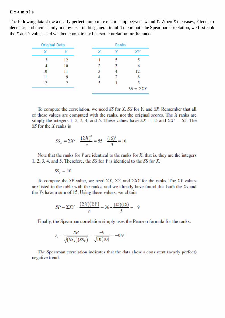
E x a m p l e

The following data show a nearly perfect monotonic relationship between X and Y. When X increases, Y tends to

decrease, and there is only one reversal in this general trend. To compute the Spearman correlation, we first rank

the X and Y values, and we then compute the Pearson correlation for the ranks.

3. Pearson’s ϕ correlation

When both variables (X and Y) measured for each individual are dichotomous, the correlation between the two

variables is called the phi-coefficient. To compute phi (ϕ), you follow a two-step procedure:

1. Convert each of the dichotomous variables to numerical values by assigning a 0 to one category and a 1 to the

other category for each of the variables.

2. Use the regular Pearson formula with the converted scores.

E x a m p l e

A researcher is interested in examining the relationship between birth-order position and personality for

individuals who have at least one sibling. A random sample of n = 8 participants is obtained, and each individual

is classified in terms of birth-order position as first-born versus later-born. Then, each individual’s personality is

classified as either introvert or extrovert. The original measurements are then converted to numerical values by

the following assignments:

The original data and the converted scores are as follows:

The Pearson correlation formula is then used with the converted data to compute the phi-coefficient.

4.The Point-Biserial Correlation

The point-biserial correlation is used to measure the relationship between two variables in situations in which

one variable consists of regular, numerical scores, but the second variable has only two values. A variable with

only two values is called a dichotomous variable or a binomial variable.

To compute the point-biserial correlation, the dichotomous variable is first converted to numerical values by

assigning a value of zero (0) to one category and a value of one (1) to the other category. Then, the regular

Pearson correlation formula is used with theconverted data.