Atmos. Meas. Tech., 5, 2569–2579, 2012www.atmos-meas-tech.net/5/2569/2012/doi:10.5194/amt-5-2569-2012© Author(s) 2012. CC Attribution 3.0 License.

AtmosphericMeasurement

Techniques

Correction of static pressure on a research aircraft in acceleratedflight using differential pressure measurements

A. R. Rodi and D. C. Leon

Department of Atmospheric Science, University of Wyoming, Laramie, Wyoming, USA

Correspondence to:A. R. Rodi (rodi@uwyo.edu)

Received: 9 April 2012 – Published in Atmos. Meas. Tech. Discuss.: 21 May 2012Revised: 14 September 2012 – Accepted: 17 September 2012 – Published: 1 November 2012

Abstract. A method is described that estimates the error inthe static pressure measurement on an aircraft from differen-tial pressure measurements on the hemispherical surface ofa Rosemount model 858AJ air velocity probe mounted on aboom ahead of the aircraft. The theoretical predictions forhow the pressure should vary over the surface of the hemi-sphere, involving an unknown sensitivity parameter, leads toa set of equations that can be solved for the unknowns – angleof attack, angle of sideslip, dynamic pressure and the error instatic pressure – if the sensitivity factor can be determined.The sensitivity factor was determined on the University ofWyoming King Air research aircraft by comparisons withthe error measured with a carefully designed sonde towedon connecting tubing behind the aircraft – a trailing cone –and the result was shown to have a precision of about±10 Paover a wide range of conditions, including various altitudes,power settings, and gear and flap extensions. Under acceler-ated flight conditions, geometric altitude data from a com-bined Global Navigation Satellite System (GNSS) and iner-tial measurement unit (IMU) system are used to estimate ac-celeration effects on the error, and the algorithm is shown topredict corrections to a precision of better than±20 Pa underthose conditions. Some limiting factors affecting the preci-sion of static pressure measurement on a research aircraft arediscussed.

1 Introduction

Static pressure measurement on an aircraft is inherently prob-lematic because the pressure changes as the air acceleratesaround the wings and fuselage, as predicted by the Bernoulliequation. It is difficult to find a location on the aircraft tomeasure the true undisturbed pressure,P∞, i.e., the pressure

at a distance far from the flow-disturbing effects. On the air-craft, static pressurePs is measured at a set of ports wherethe aircraft designers have determined that the error, re-ferred to as thestatic defector position error, is minimal.In addition to causing errors in pressure-derived aircraft alti-tude, the static defect also leads directly to errors in airspeedand other measurements that need dynamic corrections, suchas temperature, for example. In the pitot tube technique ofairspeed measurement (Doebelin, 1990), dynamic pressureqc = PT−Ps ' 1/2ρU2 is sensed, wherePT is the total pres-sure,ρ the air density, andU the airspeed. On the Universityof Wyoming King Air (UWKA) research aircraft, static pres-sure errors can be as large as 2 % ofqc at research aircraftspeeds (∼ 100 m s−1), and this error transfers directly to anerror of 1 % (1 m s−1) in airspeed. These errors directly affectestimates of atmospheric air motions which are sensed usingthe “drift method” in which the three-dimensional airspeedand ground velocity vectors are subtracted.

The static pressure ports on the UWKA are located on bothsides of the fuselage near the rear of the aircraft. The ports areconnected together in a manifold to compensate for the rampressure effect that sideslipping can create on the upstreamside of the fuselage. By manifolding, it is assumed that thiseffect will average to zero. But when lateral airspeed compo-nents occur because of turbulence, or by rudder applicationcausing sideslipping, this assumption may not be correct, asis shown later in this paper. Further, these errors are likely tochange with the deployment of wing flaps, landing gear, orthe addition of external housings and fairings used to accom-modate instruments. The usual approach is to develop cor-rections using data taken from flights past an instrumentedtower, or from precise static pressure sources towed behindthe aircraft (Brown, 1988; Wendisch and Brenguier, 2013).

Published by Copernicus Publications on behalf of the European Geosciences Union.

2570 A. R. Rodi and D. C. Leon: Correction of static pressure on a research aircraft

Static pressure becomes more problematic when aircraftare used in the study of pressure fields in baroclinic zonesor cloud systems.Bellamy (1945) introduced airborne de-termination of D-value, the difference between the radar-determined geometric altitude and the pressure altitude fromstatic pressure, using the standard atmosphere assumption.Shapiro and Kennedy(1981) and Brown et al.(1981) ap-plied this to the determination of jet stream geostrophic andageostrophic winds. This pressure gradient approach has alsobeen used for studies of low-level jets (Rodi and Parish,1988; Parish et al., 1988; Parish, 2000). LeMone and Tar-leton (1986) and LeMone et al.(1988) used altitude de-rived from accelerometer measurements instead of radar al-titude in perturbation pressure studies around clouds sug-gesting that accuracies of 20 Pa can be obtained, but onlywith substantial empirical corrections and carefully flownlegs. More recently,Parish et al.(2007) andParish and Leon(2012) demonstrated that Global Navigation Satellite System(GNSS, hereafter referred to as global positioning system –GPS) data can resolve both pressure gradients and perturba-tions associated with mesoscale and cloud-scale systems.

In this study, we develop and test a method for estimatingstatic defect using differential pressure measurements on thehemispherical leading surface of a Rosemount model 858AJ(hereafter R858) air velocity probe. The theoretical predic-tions for how the pressure should vary (presented in the Ap-pendix) lead to a set of equations that can be used to solve thestatic pressure error in addition to the attack angle, sideslipangle and dynamic pressure. We first use trailing sonde datato determine the probe sensitivity factor, and then compareresulting error estimates with accurate altitude measurementsfrom a GPS-aided inertial measurement unit (IMU), allowingfor an independent check of the precision of the algorithmand an examination of the effects of aircraft acceleration.

2 Retrieval of static pressure error from differentialpressure measurements

Bogel and Baumann(1991) describe a method of analysis ofR858 measurements during pilot-induced maneuvers to esti-mate static pressure errors.Crawford and Dobosy(1992) de-scribe the Best Aircraft Turbulence (BAT) differential pres-sure flow-angle probe which addresses the static pressureproblem by averaging pressure on several ports. Here, wedevelop a method to predict the static pressure error directlyby using pressure measurements from the R858 air veloc-ity probe which, on the UWKA, is mounted at the tip ofa boom, as shown in Fig.1. The probe is a hemisphere-cylinder configuration in which a hemispherical surface isat the end of a 2.5 cm diameter, 12.5 cm long cylindricalsection. Pressure measurements on ports in a hemispheri-cal surface are used for airspeed and flow angle determina-tion (Brown et al., 1983). There are 5 ports: one central portwhich approximates total pressure, two ports separated by

Fig. 1.UWKA showing nose boom location.

±45◦ from the central axis in the aircraft horizontal planefor sideslip angle determination, and two ports separated by±45◦ in the aircraft vertical plane for attack angle determi-nation.

In the UWKA system, four differential pressure measure-ments are made, allowing the static error to be estimated. Themethod and specific equations used in the UWKA R858 con-figuration are presented in the Appendix. The attack angleα,for example, can be estimated as described in the manufac-turer’s technical note (Rosemount, 1976) using

α 'Pα1 − Pα2

Kqc

(1)

where the numerator is the differential pressure between thetwo attack angle ports. The sensitivity coefficient, assumingpotential flow (using a sensitivity factor, as defined in theAppendix,f = 9/4) for small angles, isK ∼= 2f (π/180) =

0.0785 deg−1. Brown et al.(1983) investigatedK using datafrom flight maneuvers for the R858 on the noseboom on theNCAR Sabreliner. They found that forNMach < 0.5, K =

0.068 deg−1 (f = 1.95), 13 % lower than the value recom-mended inRosemount(1976). This determination ofK wasnot exact nor without ambiguities, however. TheBrown et al.(1983) method substituted precise IMU-measured pitch an-gle for attack angle, which is valid during periods of straightand level flight assuming zero vertical wind and aircraft ver-tical velocity. Using pitch in this manner, the upwash effect(Crawford et al., 1996) of the fuselage, wings, and possiblythe R858 itself is incorporated into the value ofK. The senseof upwash effect is to make the local attack angle larger thanthe pitch angle, causingK to be overestimated compared tothe local value ofK without the upwash effect.Brown et al.(1983) apparently also used1P1 for q without static defector flow angle correction, which could further bias the K-values reported. In the present study, the sensitivity factor is

Atmos. Meas. Tech., 5, 2569–2579, 2012 www.atmos-meas-tech.net/5/2569/2012/

A. R. Rodi and D. C. Leon: Correction of static pressure on a research aircraft 2571

Fig. 2. Scatter plots (10 Hz data) as functions of attack angle [deg] for various flight configurations and altitudes as indicated in legends:(a) dynamic pressureqc [hPa],(b) and(c) static pressure error [Pa] determined by TC, and(d) Mach number.

estimated directly so that the upwash effect is not accountedfor so that the flow angles that result are relative to the hemi-spherical surface, andq is corrected for flow angle.

We now show that the static pressure error can be deter-mined from the differential pressure measurements, assum-ing that sensitivity factorf can be determined. The theoret-ical predictions of the four differential measurements fromthe Appendix (Eq. A11) are:

1P1 = P1 − Ps,m= q[1− (f − 1)(tan2α + tan2β)/

(1+ tan2α + tan2β)] −Perr

1Pα = P4 − P5 = 2f q tanα/(1+ tan2α + tan2β)

1Pβ = P2 − P3 = 2f q tanβ/(1+ tan2α + tan2β)

1PR = P1 − P2 = f q(1− 2tanβ − tan2β)/

2(1+ tan2α + tan2β)

(2)

where here we have replacedP∞ in Eq. (A11) with the mea-sured static pressurePs,m less the unknown errorPerr, and theremaining unknowns are the attack angleα, sideslip angleβ,dynamic pressureq, and the probe sensitivityf .

We note that we are solving for the error, using the expres-sion for1P1 in Eq. (2) rearranged as

Perr = q[1− (f − 1)(tan2α + tan2β)/

(1+ tan2α + tan2β)] −1P1. (3)

We show in the Appendix thatα andβ can be found with-out a priori knowledge off . Thus,Perr is the departure of1P1 from q after the attack and sideslip angle correction.The strategy is to develop an estimatef using the trailing

Fig. 3. Scatter plots (10 Hz data) of probe sensitivity factorf , cal-culated from the solution of Eq. (2), versus1Pα [hPa] (top panel),and Mach number (bottom panel) for various flight configurationsand altitudes, as indicated in legend.

cone test data, described in the next section, and then es-timatePerr as one of the unknowns from the four pressuremeasurements.

www.atmos-meas-tech.net/5/2569/2012/ Atmos. Meas. Tech., 5, 2569–2579, 2012

2572 A. R. Rodi and D. C. Leon: Correction of static pressure on a research aircraft

Fig. 4.Pressure error[Pa] predicted from differential pressure algo-rithm vs. error measured with TC for various flight configurations,altitudes and propellor speeds, as indicated in legends (10 Hz data).1 : 1 lines are shown.

3 Trailing cone test data

Ikhtiari and Marth(1964) andMabry and Brumby(1968) de-scribe an aircraft pressure calibration system in which a staticpressure probe, connected to the aircraft by tubing, is towedat some distance behind and below the aircraft, away fromthe disturbing influence of the aircraft. The towed sonde isstabilized in flight by means of a carefully engineered cone– thus the term “trailing cone” (hereafter called TC ) – thatcreates drag for stabilization of static pressure ports whichare distributed around the circumference of a straight pieceof tubing behind the cone.Brown (1988) described the tech-nique in detail, and demonstrated for the NCAR Sabrelinerthat the largest expected error in the pressure measurementis ±39 Pa after application of corrections based upon the TCdata. The distance that the TC is extended is chosen to belong enough to minimize pressure fluctuations in the air-craft’s wake. However, accelerations cause errors. For ex-ample, with a 19 m tubing length (the length used for theUWKA), a 0.1 g acceleration will result in a 15 Pa effect.Consequently, we limit data collection to steady, straightflight legs.

A UWKA test flight using the Douglas model 501 TC wasconducted on 27 October 2005. Data were collected in sev-eral configurations: (1) with the aircraft in “clean” configu-ration (landing gear raised, flaps retracted), (2) in segmentswith gear lowered, (3) with gear lowered and flaps extendedin approach mode, and (4) at different power settings and al-titudes. Several measured variables are shown in Fig.2 asa function of aircraft attack angle, using data filtered at 5 Hzand output at 10 Hz. The lack of a single relationship for allconfigurations among dynamic pressure, pressure error, andNMach is evident. This is the main obstacle to simple correc-tions as a function of one variable such as dynamic pressureor attack angle.

Fig. 5.Distribution of residual error (DP algorithm prediction minusTC measurement)[Pa] (10 Hz data).

4 Empirical determination of f from trailing cone data

We first solved Eq. (2) for the unknown values off , α, β,andqc using TC flight measurements ofPerr and differen-tial pressures1P1, 1Pα, 1Pβ , and1PR. The resulting f-values are plotted in Fig.3, and show increases with1Pα,and decreases withNMach. We then used a non-linear regres-sion procedure to obtain the empirical estimate off that bestpredicts the TC-determinedPerr. The best fit was found bytrial and error selection of variables to be:

f = c0 + c1NMach+ c2N2Mach+ c31Pα (4)

where the constants were found to bec0 = 1.700, c1 =

−0.1569, c2 = 0.06633 andc3 = +0.001254, and where1Pα is in units of hPa. A discussion of the physical basisfor these relationships will be presented later.

The resulting predictions of pressure error are comparedwith TC measurements in Fig.4 at various steady flight con-figurations and power settings. The distribution of the resid-ual errors is shown in Fig.5 to have a precision±10 Pa in allconfigurations (σ = 8 Pa).

There is additional evidence for the variability off .Brown et al. (1983) and Rosemount(1976) provide ex-perimental evidence forf decreasing withNMach, consis-tent with the present results.Traub and Rediniotis(2003)(TR03) present an analytical prediction of surface pressuresfor a hemisphere-cylinder configuration similar to the R858,and wind tunnel results at Reynolds numbers about a fac-tor of two higher than UWKA flight (NRe ≈ 1.5× 104). TheTR03 theoretical formulation, confirmed by their wind tun-nel results, predicts sensitivity to bef = 2.07 at zero in-cidence angle, and also their data show that the sensitivityvaries with incidence angle.

To explore the effect of probe shape onf , we used acommercially-available finite-element solver for turbulent,

Atmos. Meas. Tech., 5, 2569–2579, 2012 www.atmos-meas-tech.net/5/2569/2012/

A. R. Rodi and D. C. Leon: Correction of static pressure on a research aircraft 2573

Fig. 6.Models of aircraft and boom configurations (see text).

compressible flow equations (FIDAP, Fluid Dynamics Inter-national, Inc.). An axisymmetric, compressible model at zeroattack angle was used and showed thatf is different for var-ious mounting configurations, and changes with speed. So-lutions were found forNMach equivalent to speeds of 50–180 ms−1. Four configurations were modeled as shown inFig. 6 (not to scale): (1) a sphere (not shown); (2) the R858probe mounted on the end of the UWKA nose boom, which is0.2 m in diameter; (3) the spherical radome (nose radar cov-ering) as on the former National Science Foundation (NSF)King Air aircraft (N308D); and (4) the R858 mounted ona nose boom four times the diameter of the actual UWKAnose boom. Pressure distributions on the spherical surfacewere fit using the sin2 relationship (A1), and the result-ing f for eachNMach plotted in Fig.7a. For the sphere,fvaries from 1.9–2.1. Adding the nose boom behind the R858hemisphere-cylinder decreasesf to about 1.9. Increasing theboom diameter to 0.8 m lowersf to about 1.5. These resultssuggest that there is no unique value off for all mountingconfigurations of the R858. Indeed, the fuselage of the air-craft itself presents a formidable aerodynamic barrier to theprobe, which is likely to contribute to the actualf variabilityin addition to a particular mounting configuration.

To explore further the behavior off , we constructeda physical model of the R858 with extra pressure ports drilledso that adequacy of the sin2 relationship between angle andpressure could be determined by direct measurement alongwith determination off . The test was conducted in the Uni-versity of Wyoming Low Speed Wind Tunnel, which hasa test section of 0.6×0.6×0.9 m. The model was constructed75 % larger than the actual probe so that the Reynolds num-ber at the test speed of 50 m s−1 would be approximatelythat of the actual (0.0254 m diameter) probe at 90 m s−1,the typical flight speed for the UWKA. Data were digi-tized with a personal-computer-based data logging system at10 Hz after analog filtering with cutoff frequency of 2 Hz.

Fig. 7. Estimation of sensitivity factorf from (a) modeling and(b) values fromBrown et al.(1983), (Rosemount, 1976), and so-lution to Eq. (A11) for UW King Air flight data. The point labeled“T ” represents the value from determined from the wind tunnel testsof the R858 model.

The analysis then was performed on one minute averages ofpressures at each port. Additional measurements made witha standard pitot tube placed upwind from the test body toensure that the tunnel speed did not change during runs ateach attack angle. In Fig. 7b, the sensitivity off to Nmachfrom Brown et al.(1983) and (Rosemount, 1976) are shown,along withf determined from the wind tunnel tests (pointlabeled as “T ”), and the solution of Eq. (2) with actual KingAir flight data.

5 Measured pressure compared to pressure derivedfrom GPS altitude

While the 2005 TC test flight varied attack angle with air-speed and altitude, sideslip angles were intentionally keptnear zero to prevent lateral acceleration. In this section, theefficacy of the estimates ofPerr in an accelerating flight envi-ronment using the differential pressure solution described inthe previous section will be examined.

Differential global positioning system (dGPS) techniquesuse data from one or more stationary reference or baseGPS stations which have precisely determined location torefine position estimates for the receiver on the aircraft.dGPS processing techniques using dual-frequency (L1/L2)carrier phase data can eliminate errors caused by ionosphericand tropospheric delays entirely, resulting in position esti-mates with accuracy of centimeters under optimal conditions(Parish et al., 2007).

In the present study, we use post-processed inertial mea-surement unit (IMU) data in conjunction with dual-frequencydGPS data to resolve the aircraft position and motion

www.atmos-meas-tech.net/5/2569/2012/ Atmos. Meas. Tech., 5, 2569–2579, 2012

2574 A. R. Rodi and D. C. Leon: Correction of static pressure on a research aircraft

Fig. 8. Time series of(a) height difference (geometric-pressure)[m], (b) attack angle [deg],(c) sideslip angle [deg], and(d) pres-sure deviation from lever arm correction [Pa]. Time series is theconcatenation of four 500 s segments, the first two flown at 4600 m,the second two at 7000 m.

(Trimble/Applanix model AV410). The IMU data, recordedat 200 Hz, were corrected in post-processing using Trim-ble/Applanix POSPac software which implements a tightly-coupled Kalman filter between the IMU and dGPS data.The processing fully removed all L1/L2 cycle ambiguitiesin a fixed, narrow lane processing mode. Position accuracyestimated by the manufacturer is shown in Table 1. The re-sulting 200 Hz values of aircraft position and attitude werelow-pass filtered with a cutoff frequency of 10 Hz and thendecimated to 20 Hz for the present analysis. Also, accuratetime synchronization of the IMU and pressure measurementswas assured by GPS time stamping of all data.

Static pressure was measured with the Rosemount 1501High Accuracy Digital Sensing Module (HADS) which hasstatic accuracy of 20 Pa and a digital resolution of 1.8 Pa.The accuracy includes effects of non-linearity, repeatability,temperature (−51 to 80◦C) and calibration. Worst case errorfrom transducer acceleration is specified to be 20 Pa underacceleration of 6 g; the maximum acceleration in these testswas±1 g. We estimate the maximum dynamic errors in theconnecting tubing to be 10 Pa for longitudinal accelerations(here 0.1 g, 10 m tubing length) and lateral (1 g, 1 m tubinglength) accelerations of the air column.

Flight data were collected on 16 September 2011 duringpilot-induced maneuvers inducing variations in attack andsideslip angles. Periods of turns were not considered in theanalysis. The aircraft was flown at nominally constant pres-sure with deviations corrected hydrostatically to that pressureusing the method described by Parish et al. (2007). Pressure-derived altitude changes were determined from integration ofthe hydrostatic equation:

Fig. 9. Scatter plots of: (top panel) attack angle [deg] vs. verticalacceleration [m s−2]; and (bottom panel) sideslip angle [deg] vs.lateral acceleration [m s−2].

Table 1. Trimble/Applanix airborne positioning system perfor-mance specifications.

AV410 Absolute Accuracy Post-processed

Position (m) 0.05–0.30Velocity (m s−1) 0.005Roll and Pitch (deg) 0.008True Heading (deg) 0.025

AV410 Relative Accuracy

Noise (deg h−0.5) < 0.1Drift (deg h−1)∗ 0.5

∗ Attitude will drift at this rate up to the maximum absoluteaccuracy.

z − z0 = −

P∫P0

RdryTv

gdlnP (5)

wherez0 is a direct measurement of geometric altitude fromthe IMU/dGPS system at pressureP0 and virtual temperatureTv. Data were collected at two altitudes – nominally 4600 and7000 m m.s.l. Other relevant measurements include in-housedeveloped reverse flow temperature (accuracy of 0.5 K, reso-lution of 0.006 K), and Edgetech Model 137 dew point tem-perature (accuracy of 1 K, resolution 0.006 K).

A bias is introduced if an atmospheric horizontal pressuregradient exists, or when pressure is falling, along the flighttrack since constant geometric height is no longer constantpressure. To minimize this effect, the time series is broken upinto 500 s segments and reinitialized withz0 from the highlyaccurate IMU/dGPS geometric altitude value at that instant.

Atmos. Meas. Tech., 5, 2569–2579, 2012 www.atmos-meas-tech.net/5/2569/2012/

A. R. Rodi and D. C. Leon: Correction of static pressure on a research aircraft 2575

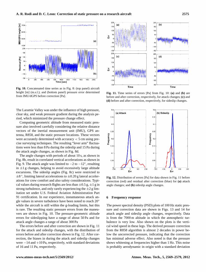
Fig. 10. Concatenated time series as in Fig.8: (top panel) aircraftheight [m] (m.s.l.); and (bottom panel) pressure error determinedfrom IMU/dGPS before correction [Pa].

The Laramie Valley was under the influence of high pressure,clear sky, and weak pressure gradient during the analysis pe-riod, which minimized the pressure change effect.

Computing geometric altitude from measured static pres-sure also involved carefully considering the relative distancevectors of the inertial measurement unit (IMU), GPS an-tenna, R858, and the static pressure locations. These vectorswere accurately determined with accuracy< 5 cm using pre-cise surveying techniques. The resulting “lever arm” fluctua-tions were less than 8 Pa during the sideslip and 15 Pa duringthe attack angle changes, as shown in Fig.8d.

The angle changes with periods of about 10 s, as shown inFig.8b, result in correlated vertical accelerations as shown inFig. 9. The attack angle was limited to−2 to−12◦, resultingin ±1 g changes, helping to avoid excessively large altitudeexcursions. The sideslip angles (Fig.8c) were restricted to±8◦, limiting lateral accelerations to±0.20 g lateral acceler-ations for crew comfort and also safety considerations. Typi-cal values during research flights are less than±0.5 g,±1 g instrong turbulence, and only rarely experiencing the±2 g lim-itation set under U.S. Federal Aviation Administration Part91 certification. In our experience, instantaneous attack an-gle values in severe turbulence have been noted to reach 20◦

while the aircraft is still within the g-loading limits, but thisis rare. The resulting static pressure errors from the maneu-vers are shown in Fig.10. The pressure-geometric altitudeerrors for sideslipping have a range of about 50 Pa and forattack angle changes a range of about 300 Pa

The errors before and after correction are shown in Fig.11for the attack and sideslip changes, with the distribution oferrors before and after correction shown in Fig.12. After cor-rection, the biases in during the attack and sideslip changeswere−14 and+10 Pa, respectively, with standard deviationsof 16 and 11 Pa, respectively.

Fig. 11. Time series of errors[Pa] from Fig. 10: (a) and (b) arebefore and after correction, respectively, for attack changes;(c) and(d) before and after correction, respectively, for sideslip changes.

Fig. 12.Distribution of errors [Pa] for data shown in Fig.11 beforecorrection (red) and residual after correction (blue) for(a) attackangle changes; and(b) sideslip angle changes.

6 Frequency response

The power spectral density (PSD) plots of 100 Hz static pres-sure and correction data are shown in Figs.13 and 14 forattack angle and sideslip angle changes, respectively. Datais from the 7000 m altitude in which the atmospheric tur-bulence is very low. Also shown on the plots is the verti-cal wind speed in these legs. The derived pressure correctionfrom the R858 algorithm is almost 2 decades in power be-low the uncorrected pressure, indicating that the correctionhas minimal adverse effect. Also noted is that the pressureshows whitening at frequencies higher than 1 Hz. This noiseis probably aerodynamic in origin with a standard deviation

www.atmos-meas-tech.net/5/2569/2012/ Atmos. Meas. Tech., 5, 2569–2579, 2012

2576 A. R. Rodi and D. C. Leon: Correction of static pressure on a research aircraft

Fig. 13.Power spectral density [variance/frequency unit] versus fre-quency [Hz] for period of attack angle change at 7000 m altitude.Left axis: corrected static pressure [Pa], and pressure correction[Pa]. Right axis: vertical wind component [m s−1] and inertial sub-range−5/3 slope.

Fig. 14.Power spectral density as in Fig.13 for period of sideslipangle changes at 7000 m altitude.

of about 15 Pa, which is above the whitening effect of thedigitization noise (2 Pa). The sharp disturbances at 30–40 Hzin Fig. 14 (sideslip periods) are probably due to the 4-bladedpropellers, which operate normally at about 1700 rpm.

7 Summary and discussion

An algorithm was developed to estimate static pressure errorsin steady flight using R858 differential pressure measure-ments, and tested with trailing cone data from a Universityof Wyoming King Air flight in 2005. After calibratingf us-ing the TC flight data, it was shown that the effects of speed,altitude and flight configuration (landing gear, flap extension)can be predicted toσ = 8 Pa in steady flight. To capture the

effects of acceleration, flight maneuvers were conducted andgeometric altitude from a GPS-aided inertial measurementdata were used to predict the pressure error. These resultssuggest that pressure errors can be determined with a preci-sion of±20 Pa during such maneuvers. It should be empha-sized that the precision, not the absolute accuracy, of theseestimates is addressed in this paper. The absolute accuracyof the error estimates using this method depend on this em-pirical determination off as well as other factors addressedin the present work.

Our attempts to use statistical regression analysis alone torelate the observed pressure error to flight data (NMach, qc,inertial acceleration) have not been successful. The differen-tial pressure method, however, has the advantage of beinga solution based upon the R858 equations, as presented inthe Appendix. The main weakness is that determination ofthe probe sensitivityf requires an independent means of itsdetermination. In the present study, we used the TC measure-ments to calibratef .

There are several sources of error which may be a factorin the interpretation. The effect of acceleration of the air inthe connecting tubing, which we estimate to be smaller than10 Pa, is indistinguishable from the aerodynamic cause of thestatic defect at the sensing ports. Nonetheless, the R858 pres-sure imbalance approach should capture the connecting tub-ing effect. The other factor is the error introduced by uncer-tainty in height differences between the static pressure portsat the rear of the fuselage, IMU and GPS antenna locations,and R858 probe tip. Figure8d shows this effect is< −15 Pa.

Our flow modeling suggests that the relatively low esti-mates off from the algorithm (f ∼= 1.7) may be reasonablesincef was found to decrease as the structure behind theR858 hemisphere-cylinder gets larger (Fig.7). These valuesare lower than TR03 (hemisphere-cylinder,f = 2.07) whichalso suggest thatf varies with incidence angle. It would beuseful to obtain independent confirmation of these estimates,for example, by using pitch angle as a surrogate forα at dif-fering airspeeds, as described byBrown et al.(1983). But thatapproach has limitations, as discussed in Sect. 2, especiallysince using pitch as an estimate ofα implicitly incorporatesthe upwash effect (Crawford et al., 1996) into the sensitiv-ity. Further, using a separate pitot tube measurement forq

would itself require the correction for static defect. The prob-lems extend to the horizontal with sidewash effects. Thus,we think that independently estimatingf , while desirable, isproblematic at best and beyond the scope of this paper.

One possible shortcoming of the theoretical prediction ofpressure distribution on the hemisphere, as shown in the Ap-pendix, is the a priori assumption thatf is constant, whileTR3 suggests thatf varies with attitude angle. Further, theflow modeling suggests thatf may be different for the verti-cal and lateral axes when the probe is ahead of an asymmet-rical body like an aircraft fuselage and wing. The completecharacterization of the probe would require a 3-dimensionalflow modeling of the entire aircraft with the boom and probe.

Atmos. Meas. Tech., 5, 2569–2579, 2012 www.atmos-meas-tech.net/5/2569/2012/

A. R. Rodi and D. C. Leon: Correction of static pressure on a research aircraft 2577

However, the precision with which our differential pressuremethod compares with the TC pressure reference and theIMU/GNSS altitudes belies a serious problem here.

We speculate that addition of a fifth differential pressuremeasurement to the R858 would eliminatef as an unknown.We are currently studying the choices for a fifth pressuremeasurement that optimizes the ability to resolve static pres-sure errors, and planning that modification and evaluation fora future study.

Appendix A

Derivation of differential pressure equations for aspherical 5-hole probe

The derivation of the relationships among the pressures ona 5-hole spherical probe surface and the attack and sideslipflow angles follows.Hale and Norrie(1967), Brown et al.(1983), andNacass(1992) analyzed the differential pressuresbetween ports in terms of the well-known pressure distribu-tion on a sphere in terms of the coefficient of pressureCp:

Cp =P − P∞

q= 1− f sin2φ (A1)

whereP is the pressure at solid angleφ from the stagnationpoint, P∞ is the pressure in the free stream,q ' 1/2ρU2 isthe dynamic pressure,ρ is the air density,U the speed, andf the sensitivity factor;f = 9/4 for potential flow (Lamb,1932).

A coordinate system is defined by unit vectors as follows:i

along the x-axis forward through the center port;j along they-axis to the right, andk long the z-axis down in aircraft co-ordinates. The angleφ in Eq. (A1) is the “great circle” anglebetween the stagnation point and point of pressure measure-ment at one of the five ports (Nacass, 1992). We define twomore unit vectors in terms of their direction cosines from theprobe axes: one,λ0, from the center of the probe hemispherethrough the stagnation point, and the other,λa , through thepressure port of interest. Thus,

λ0 = i cosθx0 + j cosθy0 + k cosθz0

λa = i cosθxa + j cosθya + k cosθza

(A2)

and the direction cosines for each vector are constrained bythe identity

cos2θx + cos2θy + cos2θz = 1. (A3)

Angle φ then can be found from the definition of the crossproduct of two vectors

sinφ = |λa × λ0|/|λa||λ0| (A4)

which can be expanded as

sin2φ = cos2θxa(1− cos2θx0) + cos2θya(1− cos2θy0)

+cos2θza(1− cos2θz0)

−2cosθxa cosθya cosθx0cosθy0 (A5)

−2cosθxa cosθza cosθx0cosθz0

−2cosθya cosθza cosθy0cosθz0.

The coordinate system is defined with regard to aircraft axesas follows: x-axis forward through the center port 1, y-axisright, and z-axis down. Ports 2 (positive) and 3 are in x–yplane, and ports 4 (positive) and 5 in the x–z plane. The cen-ter port then hasθxa = 0◦, cosθxa = 1 . The equations forφfor each port are then

sin2φ1 = 1− cos2θx0

sin2φ2 = (cosθx0cosθy2 − cosθy0cosθx2)2+ cos2θz0

sin2φ3 = (cosθx0cosθy3 − cosθy0cosθx3)2+ cos2θz0 (A6)

sin2φ4 = (cosθx0cosθz4 − cosθz0cosθx4)2+ cos2θy0

sin2φ5 = (cosθx0cosθz5 − cosθz0cosθx5)2+ cos2θy0,

where the first subscript on the direction cosines is the axisdirection, and the second subscript is the port number or 0being the stagnation point.

Four differential pressures are measured:P1 − P∞ whichapproximately the impact pressureqc at small angles,P2−P3in the plane of the probe horizontal axis defining the sideslipangleβ, P4−P5 in the plane of the probe vertical axis defin-ing the attack angleα, andP1 − P2 which is also a mea-sure of the impact pressure, as suggested byRosemount(1976) for their Model 858 5-hole probe. The center portthen hasθxa = 0◦, cosθxa = 1, and the remaining ports are atθ = 45◦, cosθya = cosθza =

√2/2. Combining these angles

and differential pressure definitions with Eq. (A6) applied toEq. (A1) gives the following set of equations for the differ-ential pressures:

P1 − P∞ = q[1− f (1− cos2θx0)]

P2 − P3 = 2qf cosθx0cosθy0P4 − P5 = 2qf cosθx0cosθz0

P1 − P2 =1

2qf (cos2θx0 − cos2θy0 − 2cosθx0cosθy0).

(A7)

We now define the attack angleα and sideslip angleβ asfunctions of the velocity components in terms of the directioncosines (Ux/U = cosθx0, etc.):

tanα =Uz

Ux

=U cosθz0

U cosθx0=

cosθz0

cosθx0(A8)

tanβ =Uy

Ux

=U cosθy0

U cosθx0=

cosθy0

cosθx0. (A9)

www.atmos-meas-tech.net/5/2569/2012/ Atmos. Meas. Tech., 5, 2569–2579, 2012

2578 A. R. Rodi and D. C. Leon: Correction of static pressure on a research aircraft

Note thatβ as defined here is not the standard definitionof sideslip (ISO, 1985), but is the commonly used definitionbecause of its natural relation toUy in the wind computation.

Equations (A8) and (A9) can be solved for the directioncosines as

cosθx0 = 1/(1+ tan2α + tan2β)1/2

cosθy0 = tanβ/(1+ tan2α + tan2β)1/2

cosθz0 = tanα/(1+ tan2α + tan2β)1/2

.

(A10)

Equations (A7)–(A10) can be combined to give the final setof equations, assuming exact knowledge ofP∞:

1P1 = P1 − P∞ = q[1− (f − 1)(tan2α + tan2β)/

(1+ tan2α + tan2β)]

1Pα = P4 − P5 = 2f q tanα/(1+ tan2α + tan2β)

1Pβ = P2 − P3 = 2f q tanβ/(1+ tan2α + tan2β)

1PR = P1 − P2 = f q(1− 2tanβ − tan2β)/

2(1+ tan2α + tan2β).

(A11)

Equation (A11) can be solved either numerically or analyti-cally for the unknowns tanβ, tanα, q andf . The1Pα, 1Pβ ,and 1PR equations can be solved analytically tanβ, tanαwithout a priori knowledge of dynamic pressureq or sensi-tivity factor f . Those solutions are:

tanβ = (√

2(1P 2β + 21Pβ1PR + 21P 2

R)

− 1Pβ − 21PR)/1Pβ

tanα = (tanβ)1Pα/1Pβ .

(A12)

We note that the limiting relationship when1PB → 0 is

tanα =1Pα

41PR

(A13)

and

q =1P 2

α + 81P11PR

81PR

. (A14)

Acknowledgements.This study was supported by NSF Cooper-ative Agreement AGS-0334908, and NSF Grant AGS-1034862.The authors would like to thank colleagues in the Departmentof Atmospheric Science at the University of Wyoming and theUWKA facility team for collection and processing of the data,and Prof. William Lindberg, UW Department of MechanicalEngineering, for assistance with the wind tunnel measurements andrecording. We also would like to thank an anonymous reviewerfor suggesting important improvements in the text, and also fornoticing a typographical error in the equations in the Appendix.

Edited by: P. Herckes

References

Bellamy, J. C.: The use of pressure altitude and altimeter correc-tions in meteorology, J. Meteorol., 2, 1–79,doi:10.1175/1520-0469(1945)002<0001:TUOPAA>2.0.CO;2, 1945.

Bogel, W. and Baumann, R.: Test and calibration of theDLR Falcon wind measuring system by maneuvers,J. Atmos. Ocean. Tech., 8, 5–18,doi:10.1175/1520-0426(1991)008<0005:TACOTD>2.0.CO;2, 1991.

Brown, E. N.: Position Error Calibration of a Pressure Sur-vey Aircraft Using a Trailing Cone, Tech. Rep. NCAR/TN-313+STR, National Center for Atmospheric Research, Boulder,CO,doi:10.5065/D6X34VF1, 1988.

Brown, E. N., Shapiro, M. A., Kennedy, P. J., and Friehe,C. A.: The application of airborne radar altimetry tothe measurement of height and slope of isobaric sur-faces, J. Appl. Meteorol., 20, 171–180,doi:10.1175/1520-0450(1981)020<1070:TAOARA>2.0.CO;2, 1981.

Brown, E. N., Friehe, C. A., and Lenschow, D. H.: The useof pressure fluctuations on the nose of an aircraft for mea-suring air motion, J. Clim. Appl. Meteorol., 22, 1070–1075,doi:10.1175/1520-0450(1983)022<0171:TUOPFO>2.0.CO;2,1983.

Crawford, T. L. and Dobosy, R. J.: A sensitive fast-response probeto measure turbulence and heat-flux from any airplane, Bound.-Lay. Meteorol., 59, 257–278,doi:10.1007/BF00119816, 1992.

Crawford, T. L., Dobosy, R. J., and Dumas, E. J.: Aircraft windmeasurement considering lift-induced upwash, Bound.-Lay. Me-teorol., 80, 79–94,doi:10.1007/BF00119012, 1996.

Doebelin, E. O.: Measurement systems: application and design,McGraw-Hill, New York, 4th Edn., ISBN: 978-0070173385,1990.

Hale, M. R. and Norrie, D. H.: The analysis and calibration the five-hole spherical pitot, Tech. Rep. ASME Publication 67-WA/FE-24, Amer. Soc. Mech. Eng., New York, 1967.

Ikhtiari, P. A. and Marth, V. G.: Trailing cone static pressure mea-surement device, J. Aircraft, 1, 93–94,doi:10.2514/3.43563,1964.

ISO: Flight dynamics, concepts and quantities Part 2: Motions ofaircraft and the atmosphere relative to the earth, 2nd Edn., Ref.No. ISO 1151/2-1985(E), International Organization for Stan-dardization, Geneva, Switzerland, 1985.

Lamb, H.: Hydrodynamics, Dover Publications, New York,ISBN: 978-0486602561, 1932.

LeMone, M. A. and Tarleton, L. F.: The use of inertial altitudein the determination of the convective-scale pressure field overland, J. Atmos. Ocean. Tech., 3, 650–661,doi:10.1175/1520-0426(1986)003<0650:TUOIAI>2.0.CO;2, 1986.

LeMone, M. A., Tarleton, L. F., and Barnes, G. M.: Per-turbation pressure at the base of cumulus clouds in lowshear, Mon. Weather Rev., 116, 2062–2068,doi:10.1175/1520-0493(1988)116<2062:PPATBO>2.0.CO;2, 1988.

Mabry, G. and Brumby, R.: DC-8 Airspeed Static Position ErrorRepeatability, Tech. Rep. Douglas Paper 5517, Douglas AircraftCo., Unk., 1968.

Nacass, P. L.: Theoretical Errors on Airborne Measurements of:Static Pressure, Impact Temperature, Air Flow Angle, Air FlowSpeed, Tech. Rep. NCAR/TN-385+STR, National Center forAtmospheric Research, Boulder, CO,doi:10.5065/D6M61H79,1992.

Atmos. Meas. Tech., 5, 2569–2579, 2012 www.atmos-meas-tech.net/5/2569/2012/

A. R. Rodi and D. C. Leon: Correction of static pressure on a research aircraft 2579

Parish, T. R.: Forcing of the summertime low-level jet alongthe california coast, J. Appl. Meteorol., 39, 2421–2433,doi:10.1175/1520-0450(2000)039<2421:FOTSLL>2.0.CO;2,2000.

Parish, T. R. and Leon, D.: Measurement of cloud perturbation pres-sures using an instrumented aircraft, J. Atmos. Ocean. Tech., on-line first: doi:10.1175/JTECH-D-12-00011.1, 2012.

Parish, T. R., Rodi, A. R., and Clark, R. D.: A casestudy of the summertime Great Plains Low Level Jet,Mon. Weather Rev., 116, 94–105,doi:10.1175/1520-0493(1988)116<0094:ACSOTS>2.0.CO;2, 1988.

Parish, T. R., Burkhart, M. D., and Rodi, A. R.: Determination of thehorizontal pressure gradient force using Global Positioning Sys-tem onboard an instrumented aircraft, J. Atmos. Ocean. Tech.,24, 521–528,doi:10.1175/JTECH1986.1, 2007.

Rodi, A. R. and Parish, T. R.: Aircraft measurement ofmesoscale pressure gradients and ageostrophic winds,J. Atmos. Ocean. Tech., 5, 91–101,doi:10.1175/1520-0426(1988)005<0091:AMOMPG>2.0.CO;2, 1988.

Rosemount: Model 858 Flow Angle Sensors, Tech. Rep. Bulletin1014, Revised 4/76, Rosemount Engineering, Minneapolis, MN,1976.

Shapiro, M. A. and Kennedy, P. J.: Research aircraft mea-surements of jet stream geostrophic and ageostrophicwinds, J. Atmos. Sci., 38, 2642–2652,doi:10.1175/1520-0469(1981)038<2642:RAMOJS>2.0.CO;2, 1981.

Traub, L. and Rediniotis, O.: Analytic prediction of surface pres-sures over a hemisphere-cylinder at incidence, J. Aircraft, 40,645–652,doi:10.2514/2.3168, 2003.

Wendisch, M. and Brenguier, J. (Eds.): Airborne Measurementsfor Environmental Research, Wiley-VCH Verlag GmbH &Co. KGaA, Weinheim, Germany, ISBN: 978-3-527-40996-9, inpress, 2013.

www.atmos-meas-tech.net/5/2569/2012/ Atmos. Meas. Tech., 5, 2569–2579, 2012