correction for specimen movement and rotation errors for ... · correction for specimen movement...

Correction for specimen movement and rotation errors for in-vivo

Optical Projection Tomography

Udo Jochen Birk,1,2,3,*

Matthias Rieckher,4 Nikos Konstantinides,

4 Alex Darrell,

5,6

Ana Sarasa-Renedo,4 Heiko Meyer,

1,7 Nektarios Tavernarakis,

4 and Jorge Ripoll

1

1Institute of Electronic Structure & Laser, Foundation for Research and Technology-Hellas (FORTH), P.O Box 1527, 71110 Heraklion, Greece

2Kirchhoff Institut für Physik, Universität Heidelberg, INF 227, 69120 Heidelberg, Germany 3Medizinisches Laserzentrum Lübeck GmbH, Peter-Monnik-Weg 4, D-23452 Lübeck, Germany

4Institute of Molecular Biology and Biotechnology, FORTH, 71110 Heraklion, Greece 5Institute of Computer Science, FORTH, 71110 Heraklion, Greece

6Currently with the Medical Vision Laboratory, Department of Engineering Science, Oxford University, Parks Road, Oxford OX1 3PJ, UK

7Currently with the Laser Zentrum Hannover e.V., Hollerithallee 8, 30419 Hannover, Germany *[email protected]

Abstract: The application of optical projection tomography to in-vivo experiments is limited by specimen movement during the acquisition. We present a set of mathematical correction methods applied to the acquired data stacks to correct for movement in both directions of the image plane. These methods have been applied to correct experimental data taken from in-vivo optical projection tomography experiments in Caenorhabditis elegans. Successful reconstructions for both fluorescence and white light (absorption) measurements are shown. Since no difference between movement of the animal and movement of the rotation axis is made, this approach at the same time removes artifacts due to mechanical drifts and errors in the assumed center of rotation.

©2010 Optical Society of America

OCIS codes: (100.6950) Tomographic image processing; (170.6960) Tomography; (110.3010) Image reconstruction techniques.

References and links

1. M. J. Rust, M. Bates, and X. Zhuang, “Sub-diffraction-limit imaging by stochastic optical reconstruction microscopy (STORM),” Nat. Methods 3(10), 793–796 (2006).

2. E. Betzig, G. H. Patterson, R. Sougrat, O. W. Lindwasser, S. Olenych, J. S. Bonifacino, M. W. Davidson, J. Lippincott-Schwartz, and H. F. Hess, “Imaging intracellular fluorescent proteins at nanometer resolution,” Science 313(5793), 1642–1645 (2006).

3. S. T. Hess, T. P. Girirajan, and M. D. Mason, “Ultra-high resolution imaging by fluorescence photoactivation localization microscopy,” Biophys. J. 91(11), 4258–4272 (2006).

4. L. M. Hirvonen, K. Wicker, O. Mandula, and R. Heintzmann, “Structured illumination microscopy of a living cell,” Eur. Biophys. J. 38(6), 807–812 (2009).

5. D. Baddeley, C. Batram, Y. Weiland, C. Cremer, and U. J. Birk, “Nanostructure analysis using spatially modulated illumination microscopy,” Nat. Protoc. 2(10), 2640–2646 (2007).

6. D. Baddeley, V. O. Chagin, L. Schermelleh, S. Martin, A. Pombo, P. M. Carlton, A. Gahl, P. Domaing, U. Birk, H. Leonhardt, C. Cremer, and M. C. Cardoso, “Measurement of replication structures at the nanometer scale using super-resolution light microscopy,” Nucleic Acids Res. 38, 1–11 (2009).

7. N. Ji, D. E. Milkie, and E. Betzig, “Adaptive optics via pupil segmentation for high-resolution imaging in biological tissues,” Nat. Methods 7(2), 141–147 (2010).

8. W. Denk, J. H. Strickler, and W. W. Webb, “Two-photon laser scanning fluorescence microscopy,” Science 248(4951), 73–76 (1990).

9. C. Vinegoni, L. Fexon, P. F. Feruglio, M. Pivovarov, J. L. Figueiredo, M. Nahrendorf, A. Pozzo, A. Sbarbati, and R. Weissleder, “High throughput transmission optical projection tomography using low cost graphics processing unit,” Opt. Express 17(25), 22320–22332 (2009).

10. J. Sharpe, U. Ahlgren, P. Perry, B. Hill, A. Ross, J. Hecksher-Sørensen, R. Baldock, and D. Davidson, “Optical projection tomography as a tool for 3D microscopy and gene expression studies,” Science 296(5567), 541–545 (2002).

11. J. Sharpe, “Optical projection tomography,” Annu. Rev. Biomed. Eng. 6(1), 209–228 (2004).

#129189 - $15.00 USD Received 28 May 2010; revised 27 Jun 2010; accepted 30 Jun 2010; published 14 Jul 2010(C) 2010 OSA 2 August 2010 / Vol. 1, No. 1 / BIOMEDICAL OPTICS EXPRESS 87

12. M. J. Boot, C. H. Westerberg, J. Sanz-Ezquerro, J. Cotterell, R. Schweitzer, M. Torres, and J. Sharpe, “In vitro whole-organ imaging: 4D quantification of growing mouse limb buds,” Nat. Methods 5(7), 609–612 (2008).

13. A. Darrell, H. Meyer, K. Marias, M. Brady, and J. Ripoll, “Weighted filtered backprojection for quantitative fluorescence optical projection tomography,” Phys. Med. Biol. 53(14), 3863–3881 (2008).

14. H. Meyer, A. Darrell, A. Metaxakis, C. Savakis, and J. Ripoll, “Optical Projection Tomography for In-Vivo Imaging of Drosophila melanogaster,” Microscopy and Analysis 22, 19–22 (2008).

15. C. Vinegoni, C. Pitsouli, D. Razansky, N. Perrimon, and V. Ntziachristos, “In vivo imaging of Drosophila melanogaster pupae with mesoscopic fluorescence tomography,” Nat. Methods 5(1), 45–47 (2008).

16. J. Huisken, J. Swoger, F. Del Bene, J. Wittbrodt, and E. H. Stelzer, “Optical sectioning deep inside live embryos by selective plane illumination microscopy,” Science 305(5686), 1007–1009 (2004).

17. R. B. Schulz, J. Ripoll, and V. Ntziachristos, “Noncontact optical tomography of turbid media,” Opt. Lett. 28(18), 1701–1703 (2003).

18. A. Sarasa-Renedo, R. Favicchio, U. Birk, G. Zacharakis, C. Mamalaki, and J. Ripoll, “Source intensity profile in noncontact optical tomography,” Opt. Lett. 35(1), 34–36 (2010).

19. J. McGinty, K. B. Tahir, R. Laine, C. B. Talbot, C. Dunsby, M. A. A. Neil, L. Quintana, J. Swoger, J. Sharpe, and P. M. W. French, “Fluorescence lifetime optical projection tomography,” J Biophotonics 1(5), 390–394 (2008).

20. J. Culver, W. Akers, and S. Achilefu, “Multimodality molecular imaging with combined optical and SPECT/PET modalities,” J. Nucl. Med. 49(2), 169–172 (2008).

21. C. Vinegoni, D. Razansky, J. L. Figueiredo, L. Fexon, M. Pivovarov, M. Nahrendorf, V. Ntziachristos, and R. Weissleder, “Born normalization for fluorescence optical projection tomography for whole heart imaging,” J. Vis. Exp. 28(28), 1389 (2009).

22. A. Bassi, D. Brida, C. D'Andrea, G. Valentini, S. De Silvestri, G. Cerullo, and R. Cubeddu, “Time gated optical projection tomography for 3D imaging of highly scattering biological models,” in Biomedical Optics, OSA Technical Digest (CD) (Optical Society of America, 2010), p. BTuF5.

23. J. R. Walls, J. G. Sled, J. Sharpe, and R. M. Henkelman, “Resolution improvement in emission optical projection tomography,” Phys. Med. Biol. 52(10), 2775–2790 (2007).

24. U. J. Birk, A. Darrell, N. Konstantinides, A. Sarasa-Renedo, and J. Ripoll, “Improved Reconstructions and Generalized Filtered Back Projection for Optical Projection Tomography,” Appl. Opt. submitted.

25. A. Katsevich, “An accurate approximate algorithm for motion compensation in two-dimensional tomography,” Inverse Probl. 26(6), 065007 (2010).

26. U. J. Birk, A. Darrell, N. Konstantinides, and J. Ripoll, “Correction of Lateral Movement and Spherical Aberrations in Optical Projection Tomography,” in Biomedical Optics, OSA Technical Digest (CD) (Optical Society of America, 2010), p. BTuF6.

27. S. Brenner, “The genetics of Caenorhabditis elegans,” Genetics 77(1), 71–94 (1974). 28. J. R. Walls, J. G. Sled, J. Sharpe, and R. M. Henkelman, “Correction of artefacts in optical projection

tomography,” Phys. Med. Biol. 50(19), 4645–4665 (2005). 29. Quantitative Imaging Group at the Faculty of Applied Sciences, Delft University of Technology, “DIPimage &

DIPlib,” http://www.diplib.org/. 30. J. C. Crocker, and D. G. Grier, “Methods of Digital Video Microscopy for Colloidal Studies,” J. Colloid Interface

Sci. 179(1), 298–310 (1996). 31. L. R. Barnden, J. Dickson, and B. F. Hutton, “Detection and validation of the body edge in low count emission

tomography images,” Comput. Methods Programs Biomed. 84(2-3), 153–161 (2006). 32. A. C. Kak, and M. Slaney, Principles of Computerized Tomographic Imaging (IEEE Service Center, 1988). 33. D. Baddeley, Y. Weiland, C. Batram, U. Birk, and C. Cremer, “Model based precision structural measurements

on barely resolved objects,” J. Microsc. 237(1), 70–78 (2010).

1. Introduction

Immense improvements in optical imaging techniques are currently revolutionizing vast fields in biomedical applications, ranging from nanoscale microscopy [1–4] with nanometer precision measurements inside of cells [5,6], to deep tissue multi-photon microscopy [7,8] and optical projection tomography (OPT) [9–15] or selective plane illumination microscopy [16] for objects with a size of several millimeters, to whole animal imaging using diffuse optical tomography (DOT) [17,18]. Combinations of imaging techniques such as Fluorescence Lifetime Imaging (FLIM) together with OPT [19], or positron emission tomography (PET) together with DOT [20] help us to elucidate complex biological processes, especially when aimed at in-vivo imaging.

For imaging of small animals, embryos in early developmental stages, or parts of animals such as e.g. organs with size ranges from several tens of micrometers up to about 1 cm [21], OPT is a valuable tool as it allows non-invasive optical imaging combined with the specificity of fluorescence labeling. However, for non-transparent specimens scattering needs to be taken into account [15,22], or else it has to be reduced to a negligible amount by clearing the samples e.g. using a mixture of benzyl alcohol and benzyl benzoate [23]. So far, experiments


have been performed mostly using fixed samples. This is partly due to the optical constraints imposed on the sample, and partly due to the lack of suitable procedures to deal with specimen movement during the acquisition. While the first issue has been resolved [24], and mathematical models are presently being developed for motion correction [25], in this contribution we present a set of correction methods for object drifts in both directions of the image plane for fluorescence as well as for white light data. Whether observed drifts [26] are due to the moving specimens, or to mechanical instabilities, the presented algorithms are able to successfully detect and mathematically remove them, thus allowing 3D OPT reconstructions of live samples. Note that the presented algorithms cannot currently correct for tilts of the objects; this is the subject of ongoing research.

CCD

TLF2IOL

LED2

D

B

C

F1L

LED1

x

y

zθθθθ

CCD

TLF2IOL

LED2

D

B

C

F1L

LED1

x

y

z x

y

zθθθθ

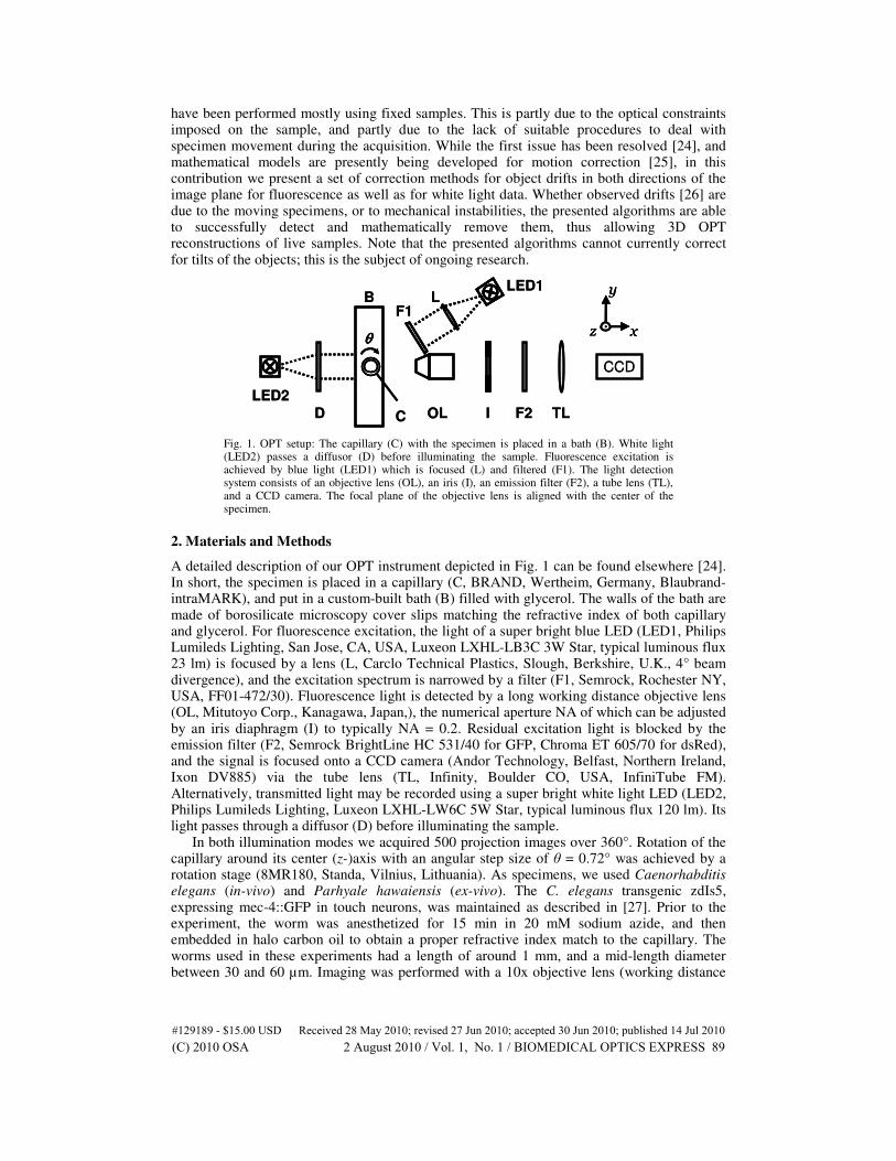
Fig. 1. OPT setup: The capillary (C) with the specimen is placed in a bath (B). White light (LED2) passes a diffusor (D) before illuminating the sample. Fluorescence excitation is achieved by blue light (LED1) which is focused (L) and filtered (F1). The light detection system consists of an objective lens (OL), an iris (I), an emission filter (F2), a tube lens (TL), and a CCD camera. The focal plane of the objective lens is aligned with the center of the specimen.

2. Materials and Methods

A detailed description of our OPT instrument depicted in Fig. 1 can be found elsewhere [24]. In short, the specimen is placed in a capillary (C, BRAND, Wertheim, Germany, Blaubrand-intraMARK), and put in a custom-built bath (B) filled with glycerol. The walls of the bath are made of borosilicate microscopy cover slips matching the refractive index of both capillary and glycerol. For fluorescence excitation, the light of a super bright blue LED (LED1, Philips Lumileds Lighting, San Jose, CA, USA, Luxeon LXHL-LB3C 3W Star, typical luminous flux 23 lm) is focused by a lens (L, Carclo Technical Plastics, Slough, Berkshire, U.K., 4° beam divergence), and the excitation spectrum is narrowed by a filter (F1, Semrock, Rochester NY, USA, FF01-472/30). Fluorescence light is detected by a long working distance objective lens (OL, Mitutoyo Corp., Kanagawa, Japan,), the numerical aperture NA of which can be adjusted by an iris diaphragm (I) to typically NA = 0.2. Residual excitation light is blocked by the emission filter (F2, Semrock BrightLine HC 531/40 for GFP, Chroma ET 605/70 for dsRed), and the signal is focused onto a CCD camera (Andor Technology, Belfast, Northern Ireland, Ixon DV885) via the tube lens (TL, Infinity, Boulder CO, USA, InfiniTube FM). Alternatively, transmitted light may be recorded using a super bright white light LED (LED2, Philips Lumileds Lighting, Luxeon LXHL-LW6C 5W Star, typical luminous flux 120 lm). Its light passes through a diffusor (D) before illuminating the sample.

In both illumination modes we acquired 500 projection images over 360°. Rotation of the capillary around its center (z-)axis with an angular step size of θ = 0.72° was achieved by a rotation stage (8MR180, Standa, Vilnius, Lithuania). As specimens, we used Caenorhabditis elegans (in-vivo) and Parhyale hawaiensis (ex-vivo). The C. elegans transgenic zdIs5, expressing mec-4::GFP in touch neurons, was maintained as described in [27]. Prior to the experiment, the worm was anesthetized for 15 min in 20 mM sodium azide, and then embedded in halo carbon oil to obtain a proper refractive index match to the capillary. The worms used in these experiments had a length of around 1 mm, and a mid-length diameter between 30 and 60 µm. Imaging was performed with a 10x objective lens (working distance


33.5mm, focal length 20mm, depth of field ca. 20 µm). With P. hawaiensis, immobilization was precipitated using a low concentration of clove oil (0.04%) in artificial sea water. After 5 min, the specimen was transferred to the capillary filled with glycerol. Typically, these animals had a length from head to tail of roughly 2.5 mm and a maximum diameter (including extremities) of about 0.6 mm when inside the capillary. Imaging of P. hawaiensis was performed using a 5x objective lens (working distance 34mm, focal length 40mm, depth of field ca. 150 µm). Since the depth of field was adjusted prior to each experiment, only typical values are given.

Although large efforts have been put in the design of the instrument and the specimens holder [24], not all mechanical instabilities could be eliminated, resulting in a drift of the complete image (corresponding to about 1 µm per hour in the object space), even when the stages were stationary (i.e. no actuation). However, movement of the sample is also expected when imaging animals in-vivo. Hence, post-acquisition correction methods need to be provided to address these issues and to correct for motion-induced blur in the final reconstructions. In general, all the correction methods described here assume the drifts to be constant for a given projection, i.e. each acquired 2D projection can be corrected by a 2D shift

vector s�

= (y,z) with independent components in y- and z-direction. However, we assume s�

to be constant for all pixels of that projection data, and only dependent on the rotation angle θ. This approach can of course be generalized by dividing each projection in multiple patches, and by treating these patches individually, since similar patching has also been shown for high-resolution truncated insets in a low resolution full reconstruction [28]. Fortunately, the movement is generally slow resulting in a strong correlation of the shifts between subsequent projections. All of the methods described below are implemented in the MATLAB programming environment (The MathWorks Inc., Natick, USA) and make use of the free DIPimage toolbox [29]. Since the lateral and the longitudinal components of the shifts are independent, we can derive correction methods for each component separately as described below.

3. Correction for longitudinal shifts

In the following, the drifts in the image plane parallel to the rotation axis are called ‘longitudinal shifts’ (z-direction in Fig. 1).

3.1 Fluorescence image data

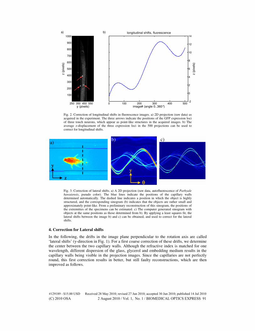
Very small fluorescent objects (point-like objects with a size equal to or smaller than the width of the point spread function [PSF] of the microscope) are used to determine drifts during the course of the experiment. The positions of these small objects can be extracted in every 2D projection using an object segmentation algorithm. A particle tracking algorithm [30] is then used to merge these positions to a 3D trajectory (y-z-position and image number). Since the z-position of the objects should be stable during the rotational actuation, the z-component of the 3D trajectory contains the values necessary to correct for longitudinal shifts. Figure 2 shows an application of such a correction in an experiment using C. elegans expressing GFP in the touch sensitivity neurons.

3.2 White light (transmission/absorption) image data

White light images taken in transmission mode usually do not show such highly structured features. Here, only very few time points can be used to correct for the longitudinal shifts. Typically the first (0° rotation angle), center (180° rotation angle), and last (360° rotation angle) are used, where the center image needs to be flipped in order to display the same view as that in the 0° and the 360° position. Using the DIPimage function ‘findshift’, the z-displacement for the three images is determined, and interpolated for the full revolution to obtain the correction values for the longitudinal shifts. From this first estimate of the longitudinal shifts, a more precise prediction can then be obtained by using a self-correcting approach (see paragraph “Self-correcting approach”).


0 100 200 300 400 500-2

0

2

4

6

8

10

12

14

image# (angle 0..360°)

z (p

ixe

ls)

longitudinal shifts, fluorescencea) b)

y (pixels)

z (p

ixe

ls)

250 350 450 550

100

200

300

400

500

600

700

800

900

1000

Fig. 2. Correction of longitudinal shifts in fluorescence images. a) 2D projection (raw data) as acquired in the experiment. The three arrows indicate the positions of the GFP expression loci of three touch neurons, which appear as point-like structures in the acquired images. b) The average z-displacement of the three expression loci in the 500 projections can be used to correct for longitudinal shifts.

a)

z

y

θ

y

b) c)a)

z

y

z

y

θ

y

θ

y

b) c)

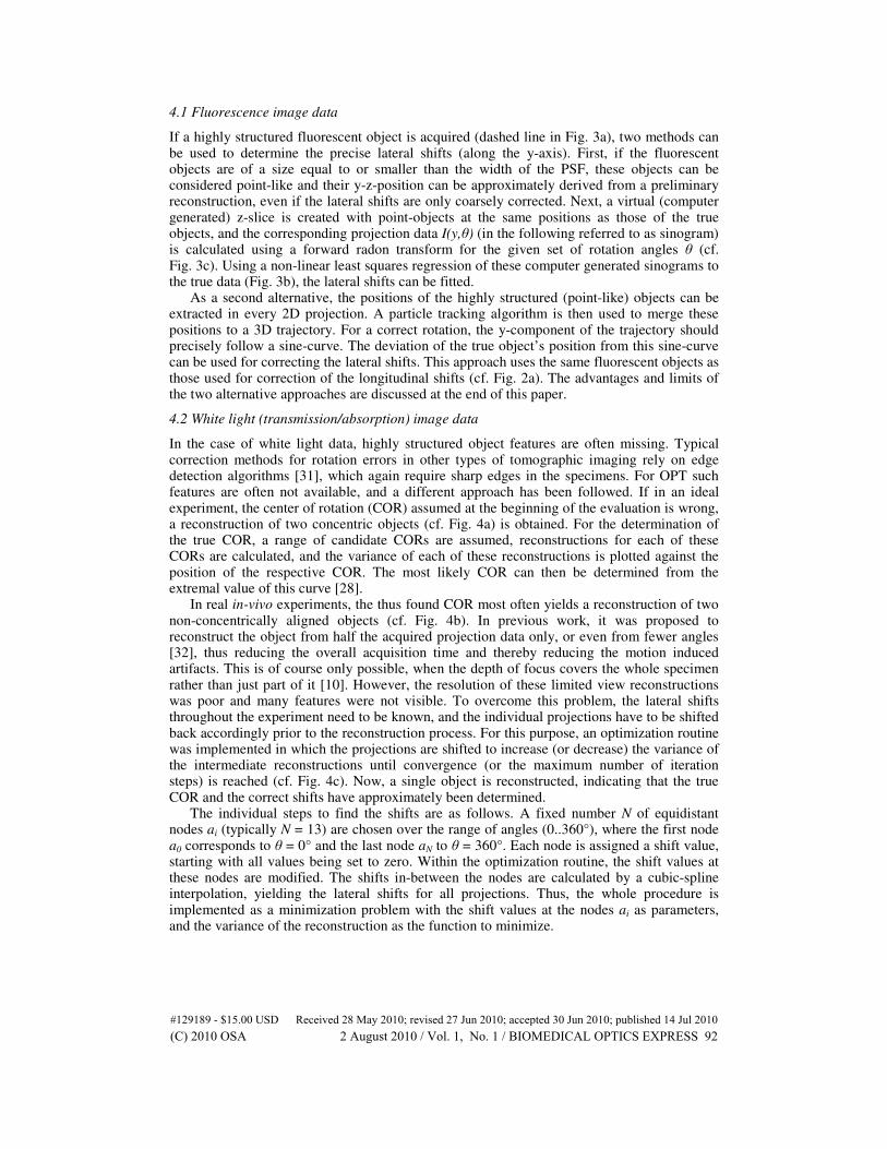
Fig. 3. Correction of lateral shifts. a) A 2D projection (raw data, autofluorescence of Parhyale hawaiensis, pseudo color). The blue lines indicate the positions of the capillary walls determined automatically. The dashed line indicates a position in which the object is highly structured, and the corresponding sinogram (b) indicates that the objects are rather small and approximately point-like. From a preliminary reconstruction of this sinogram, the positions of the extremities of the specimens can be estimated. c) The computer generated sinogram with objects at the same positions as those determined from b). By applying a least squares fit, the lateral shifts between the image b) and c) can be obtained, and used to correct for the lateral shifts.

4. Correction for Lateral shifts

In the following, the drifts in the image plane perpendicular to the rotation axis are called ‘lateral shifts’ (y-direction in Fig. 1). For a first coarse correction of these drifts, we determine the center between the two capillary walls. Although the refractive index is matched for one wavelength, different dispersion of the glass, glycerol and embedding medium results in the capillary walls being visible in the projection images. Since the capillaries are not perfectly round, this first correction results in better, but still faulty reconstructions, which are then improved as follows.


4.1 Fluorescence image data

If a highly structured fluorescent object is acquired (dashed line in Fig. 3a), two methods can be used to determine the precise lateral shifts (along the y-axis). First, if the fluorescent objects are of a size equal to or smaller than the width of the PSF, these objects can be considered point-like and their y-z-position can be approximately derived from a preliminary reconstruction, even if the lateral shifts are only coarsely corrected. Next, a virtual (computer generated) z-slice is created with point-objects at the same positions as those of the true objects, and the corresponding projection data I(y,θ) (in the following referred to as sinogram) is calculated using a forward radon transform for the given set of rotation angles θ (cf. Fig. 3c). Using a non-linear least squares regression of these computer generated sinograms to the true data (Fig. 3b), the lateral shifts can be fitted.

As a second alternative, the positions of the highly structured (point-like) objects can be extracted in every 2D projection. A particle tracking algorithm is then used to merge these positions to a 3D trajectory. For a correct rotation, the y-component of the trajectory should precisely follow a sine-curve. The deviation of the true object’s position from this sine-curve can be used for correcting the lateral shifts. This approach uses the same fluorescent objects as those used for correction of the longitudinal shifts (cf. Fig. 2a). The advantages and limits of the two alternative approaches are discussed at the end of this paper.

4.2 White light (transmission/absorption) image data

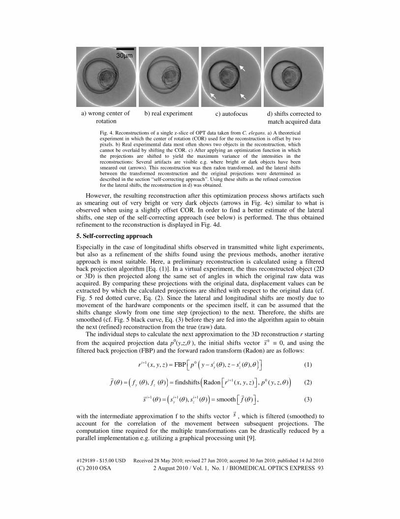
In the case of white light data, highly structured object features are often missing. Typical correction methods for rotation errors in other types of tomographic imaging rely on edge detection algorithms [31], which again require sharp edges in the specimens. For OPT such features are often not available, and a different approach has been followed. If in an ideal experiment, the center of rotation (COR) assumed at the beginning of the evaluation is wrong, a reconstruction of two concentric objects (cf. Fig. 4a) is obtained. For the determination of the true COR, a range of candidate CORs are assumed, reconstructions for each of these CORs are calculated, and the variance of each of these reconstructions is plotted against the position of the respective COR. The most likely COR can then be determined from the extremal value of this curve [28].

In real in-vivo experiments, the thus found COR most often yields a reconstruction of two non-concentrically aligned objects (cf. Fig. 4b). In previous work, it was proposed to reconstruct the object from half the acquired projection data only, or even from fewer angles [32], thus reducing the overall acquisition time and thereby reducing the motion induced artifacts. This is of course only possible, when the depth of focus covers the whole specimen rather than just part of it [10]. However, the resolution of these limited view reconstructions was poor and many features were not visible. To overcome this problem, the lateral shifts throughout the experiment need to be known, and the individual projections have to be shifted back accordingly prior to the reconstruction process. For this purpose, an optimization routine was implemented in which the projections are shifted to increase (or decrease) the variance of the intermediate reconstructions until convergence (or the maximum number of iteration steps) is reached (cf. Fig. 4c). Now, a single object is reconstructed, indicating that the true COR and the correct shifts have approximately been determined.

The individual steps to find the shifts are as follows. A fixed number N of equidistant nodes ai (typically N = 13) are chosen over the range of angles (0..360°), where the first node a0 corresponds to θ = 0° and the last node aN to θ = 360°. Each node is assigned a shift value, starting with all values being set to zero. Within the optimization routine, the shift values at these nodes are modified. The shifts in-between the nodes are calculated by a cubic-spline interpolation, yielding the lateral shifts for all projections. Thus, the whole procedure is implemented as a minimization problem with the shift values at the nodes ai as parameters, and the variance of the reconstruction as the function to minimize.


a) wrong center of

rotation

30µm

b) real experiment c) autofocus d) shifts corrected to

match acquired data

Fig. 4. Reconstructions of a single z-slice of OPT data taken from C. elegans. a) A theoretical experiment in which the center of rotation (COR) used for the reconstruction is offset by two pixels. b) Real experimental data most often shows two objects in the reconstruction, which cannot be overlaid by shifting the COR. c) After applying an optimization function in which the projections are shifted to yield the maximum variance of the intensities in the reconstructions: Several artifacts are visible e.g. where bright or dark objects have been smeared out (arrows). This reconstruction was then radon transformed, and the lateral shifts between the transformed reconstruction and the original projections were determined as described in the section “self-correcting approach”. Using these shifts as the refined correction for the lateral shifts, the reconstruction in d) was obtained.

However, the resulting reconstruction after this optimization process shows artifacts such as smearing out of very bright or very dark objects (arrows in Fig. 4c) similar to what is observed when using a slightly offset COR. In order to find a better estimate of the lateral shifts, one step of the self-correcting approach (see below) is performed. The thus obtained refinement to the reconstruction is displayed in Fig. 4d.

5. Self-correcting approach

Especially in the case of longitudinal shifts observed in transmitted white light experiments, but also as a refinement of the shifts found using the previous methods, another iterative approach is most suitable. Here, a preliminary reconstruction is calculated using a filtered back projection algorithm [Eq. (1)]. In a virtual experiment, the thus reconstructed object (2D or 3D) is then projected along the same set of angles in which the original raw data was acquired. By comparing these projections with the original data, displacement values can be extracted by which the calculated projections are shifted with respect to the original data (cf. Fig. 5 red dotted curve, Eq. (2). Since the lateral and longitudinal shifts are mostly due to movement of the hardware components or the specimen itself, it can be assumed that the shifts change slowly from one time step (projection) to the next. Therefore, the shifts are smoothed (cf. Fig. 5 black curve, Eq. (3) before they are fed into the algorithm again to obtain the next (refined) reconstruction from the true (raw) data.

The individual steps to calculate the next approximation to the 3D reconstruction r starting

from the acquired projection data p0(y,z,θ ), the initial shifts vector 0

s�

≡ 0, and using the

filtered back projection (FBP) and the forward radon transform (Radon) are as follows:

( )1 0( , , ) FBP ( ), ( ),i i i

y zr x y z p y s z sθ θ θ+ = − − (1)

( ) ( )1 0( ) ( ), ( ) findshifts Radon ( , , ) , ( , , )i

y zf f f r x y z p y zθ θ θ θ+ = = �

(2)

( )1 1 1( ) ( ), ( ) smooth ( )

i i i

y zs s s fθ θ θ θ+ + + = = �

�

, (3)

with the intermediate approximation f to the shifts vector s�

, which is filtered (smoothed) to account for the correlation of the movement between subsequent projections. The computation time required for the multiple transformations can be drastically reduced by a parallel implementation e.g. utilizing a graphical processing unit [9].


0 100 200 300 400 500-20

-10

0

10

20Lateral shifts before and after one iteration


pix

els

beforeaftersmoothed

Fig. 5. Iterative correction of (in this case) lateral shifts using a self-correcting approach. The blue curve indicates the shifts found using one of the approaches described above. After applying these shifts to the individual projections, a reconstruction is calculated. Using a forward radon transform as in a virtual experiment, this reconstruction is rotated and projections are calculated for each angle. The shifts between the thus obtained projections and the original data are determined (red dotted curve). This data is smoothed to obtain the new lateral shifts (black curve, dashed).

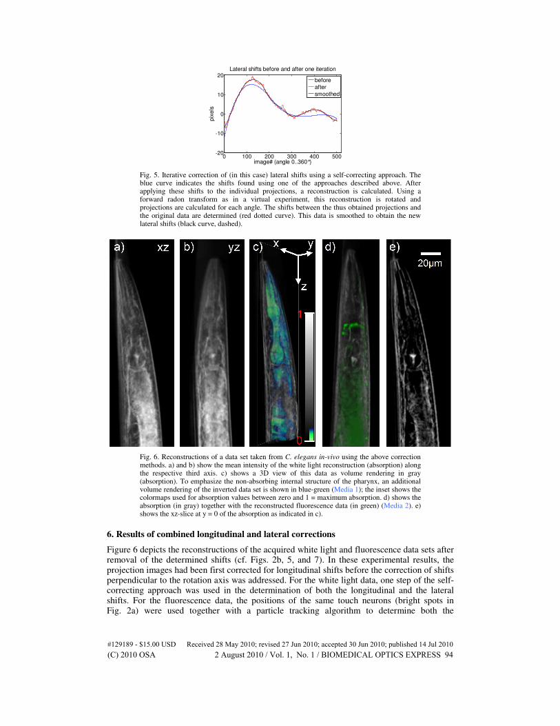
Fig. 6. Reconstructions of a data set taken from C. elegans in-vivo using the above correction methods. a) and b) show the mean intensity of the white light reconstruction (absorption) along the respective third axis. c) shows a 3D view of this data as volume rendering in gray (absorption). To emphasize the non-absorbing internal structure of the pharynx, an additional volume rendering of the inverted data set is shown in blue-green (Media 1); the inset shows the colormaps used for absorption values between zero and 1 = maximum absorption. d) shows the absorption (in gray) together with the reconstructed fluorescence data (in green) (Media 2). e) shows the xz-slice at y = 0 of the absorption as indicated in c).

6. Results of combined longitudinal and lateral corrections

Figure 6 depicts the reconstructions of the acquired white light and fluorescence data sets after removal of the determined shifts (cf. Figs. 2b, 5, and 7). In these experimental results, the projection images had been first corrected for longitudinal shifts before the correction of shifts perpendicular to the rotation axis was addressed. For the white light data, one step of the self-correcting approach was used in the determination of both the longitudinal and the lateral shifts. For the fluorescence data, the positions of the same touch neurons (bright spots in Fig. 2a) were used together with a particle tracking algorithm to determine both the


http://www.opticsinfobase.org/viewmedia.cfm?URI=boe-1-1-87-1

http://www.opticsinfobase.org/viewmedia.cfm?URI=boe-1-1-87-2

longitudinal and the lateral shifts. No additional step of the self-correcting approach was performed. Note that the white light data set was acquired after the fluorescence data set, hence different shifts were determined.

y (

pix

)white light reconstruction (x = 2)

without correction

200 400 600 800

50100150200

y (

pix

)

with correction

200 400 600 800

50100150200

fluorescence reconstruction (x = 8)

y (

pix

)

without correction

200 400 600 800 1000

100

200

z (pixels)

y (

pix

)

with correction

200 400 600 800 1000

100

200

0 100 200 300 400 500-20

-10

0

10

20shifts, white light


pix

els

(z o

r y)

0 100 200 300 400 500-20

-10

0

10

20shifts, fluorescence


pix

els

(z o

r y)

z, longitudinal

y, lateral

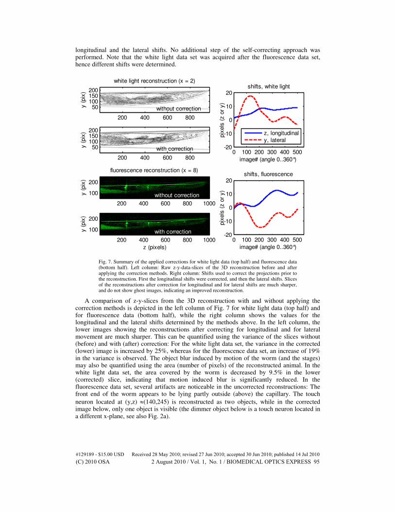
Fig. 7. Summary of the applied corrections for white light data (top half) and fluorescence data (bottom half). Left column: Raw z-y-data-slices of the 3D reconstruction before and after applying the correction methods. Right column: Shifts used to correct the projections prior to the reconstruction. First the longitudinal shifts were corrected, and then the lateral shifts. Slices of the reconstructions after correction for longitudinal and for lateral shifts are much sharper, and do not show ghost images, indicating an improved reconstruction.

A comparison of z-y-slices from the 3D reconstruction with and without applying the correction methods is depicted in the left column of Fig. 7 for white light data (top half) and for fluorescence data (bottom half), while the right column shows the values for the longitudinal and the lateral shifts determined by the methods above. In the left column, the lower images showing the reconstructions after correcting for longitudinal and for lateral movement are much sharper. This can be quantified using the variance of the slices without (before) and with (after) correction: For the white light data set, the variance in the corrected (lower) image is increased by 25%, whereas for the fluorescence data set, an increase of 19% in the variance is observed. The object blur induced by motion of the worm (and the stages) may also be quantified using the area (number of pixels) of the reconstructed animal. In the white light data set, the area covered by the worm is decreased by 9.5% in the lower (corrected) slice, indicating that motion induced blur is significantly reduced. In the fluorescence data set, several artifacts are noticeable in the uncorrected reconstructions: The front end of the worm appears to be lying partly outside (above) the capillary. The touch

neuron located at (y,z) ≈(140,245) is reconstructed as two objects, while in the corrected image below, only one object is visible (the dimmer object below is a touch neuron located in a different x-plane, see also Fig. 2a).


7. Discussion and conclusions

Two alternative methods for correcting the lateral shifts in fluorescence data have been developed. The first method relies on a comparison of a computer generated sinogram with the measured sinogram. For this method it is necessary to have multiple objects thoroughly distributed radially as well as azimuthally over the reconstructed slice, i.e. they should cover a broad range of distances to the rotation axis, and they must not be located in only one or two quadrants of the reconstructed slice. Both prerequisites need to be fulfilled in order to make the problem well-posed and thus avoid systematic errors. The second method relies on a symmetric fluorescence distribution of each segmented locus which is obviously fulfilled for point-like structures. The segmented objects need to be clearly separated (optically resolved). It can be stated that the first method is more generally applicable because any arbitrary 2D object can be constructed by placing more and more delta-peaks next to each other [33], although at the cost of longer computation times.

Additionally, the lateral shift determination method described for the white light data is suitable for fluorescence data as well, if the object structures are either not fine enough or not well enough distributed to allow the other correction methods to be applied, or when no convergence can be gained from the other two methods. This method however needs the longest computation times.

The present OPT device is now a ready-to-use microscope capable of imaging specimens both live and fixed. By the newly developed data evaluation and correction algorithms, the microscope system has been largely improved allowing routine application both in fluorescence mode, where different wavelengths for fluorescence excitation in transgenic or immunolabeled specimens are available, and in trans-illumination (white light) mode, where unique studies of anatomy and morphology are possible. We have tested our algorithms with experimental OPT data sets (white light and fluorescence) taken from C. elegans in-vivo. The correction methods presented deal successfully with the problem of movement of the animals and at the same time also with the remaining mechanical instabilities of the microscope setup. However, several assumptions have been made: First, the movement from one projection to the next is small i.e., the drifts are correlated. Second, and as a result of the first assumption, tilting of the objects during the acquisition has not been considered. However, preliminary computer simulations indicate that extraction of the object tilt is also possible (data not shown) using a similar approach i.e., by assuming a correlation of the tilts between subsequent projections.

Acknowledgments

The authors wish to acknowledge support from the European Commission (MEIF-CT-2006-041827), the Bill and Melinda Gates Foundation and the FMT-XCT FP7 EU project. AD and HM acknowledge support from EST-MolecImag MEST-CT-2004-007643. Special thanks to Michalis Averof for his help with the Parhyale hawaiensis specimens.


correction for specimen movement and rotation errors for ... · correction for specimen movement...

Documents