Corporate Tax Reform and ForeignDirect Investment in Germany -Evidence from Firm-Level Data

by

Johannes Becker�, Clemens Fuestz, Thomas Hemmelgarnx

University of Cologne

Very preliminary and incomplete conference draftDo not circulate without permission

This Version:January 2006

�Cologne Center for Public Economics, University of Cologne, Albertus-Magnus-Platz, D-50923 Cologne, Germany. E-Mail: johannes.becker@.uni-koeln.de

zCologne Center for Public Economics, University of Cologne, Albertus-Magnus-Platz, D-50923 Cologne, Germany. E-Mail: clemens.fuest@uni-koeln.de

xCologne Center for Public Economics, University of Cologne, Albertus-Magnus-Platz, D-50923 Cologne, Germany. E-Mail: thomas.hemmelgarn@uni-koeln.de

Abstract

Does the reduction of the e¤ective tax burden on corporations trigger foreign directinvestment? We take the German tax reform of 2000 as a natural experiment inorder to isolate the impact of corporate taxation on the investment of foreign-helda¢ liates in Germany. We do so by exploiting the very rich MiDi data base fromthe Deutsche Bundesbank. Although we choose an approach which is likely tounderestimate the tax e¤ects on investment we �nd signi�cant evidence that thetax reduction had the intended e¤ect of - ceteris paribus - fostering inward directinvestment. We �nd an elasticity of inward foreign direct investment with respectto the e¤ective marginal tax rate of 0.4.

JEL Codes: H25, H21

Keywords: Corporate Taxation, Foreign Direct Investment

I

1 Introduction

The strong increase in the international mobility of capital and �rms have led toenormous welfare growth in many parts of the world. However, the fast proceedingstructural change and the accelerating division of labor have forced �rm owners,employees and governments throughout the world into a permanent process ofadjustment. For governments, tax reform is one important instrument to adaptto a changing international environment. In recent years, many countries haveimplemented tax reforms which reduce the e¤ective tax burden on investment.This type of tax reform is justi�ed with the claim that it will foster domesticinvestment.Given that the border crossing mobility of capital and �rms increases, it is

reasonable to consider a reduction of the tax burden on domestic investment.But lowering the tax burden on investment necessarily implies a cut in publicexpenditure or a shift of the tax burden to other tax bases like e.g. labor orconsumption. Sound tax policy has to carefully weigh the bene�ts of a corporatetax reduction to the economy as a whole against the cost.1 Therefore, public�nance economists should seek to provide information on both the cost of taxreforms - i.e. revenue losses - and the bene�t - i.e. more investment, more jobsetc.The purpose of this paper is to measure the bene�ts of corporate tax reduction

in the form of additional inward investment of foreign owned �rms. We do so byanalyzing the e¤ect of the German tax reform in 2000, which came into force inJanuary 2001. This reform abolished the full imputation system of dividend taxa-tion and replaced it by a classical-type system. In addition, it implied substantialcorporate tax rate cuts and broadened the corporate tax base. A frequently citedgoal of the tax reform was to attract foreign direct investment in order to mitigatethe huge unemployment rate. Now, �ve years after the reform, we ask whetherthe tax reform reached this goal and whether the resulting investment increasesare worth the losses in tax revenue.We analyze this question by using the very rich MiDi data set from the Deutsche

Bundesbank with �rm-speci�c balance sheet data. Our analysis contributes toa literature that tries to clarify the incentive e¤ects of existing tax systems oncorporate investment. As corporate investment is assumed to be crucial for thegeneration of new jobs and growth, we think that this question is at the heart offuture debates on corporate tax reforms.Figure 1 illustrates the increasing importance of cross-border investment. It

shows the inward �ows (left scale) and stocks (right scale) of foreign direct invest-

1For recent surveys on the theory of capital tax competition see e.g. Wilson & Wildasin(2004) or Fuest, Huber & Mintz (2005).

1

ment in Europe.

0

100.000

200.000

300.000

400.000

500.000

600.000

700.000

800.000

1980 1982 1984 1986 1988 1990 1992 1994 1996 1998 2000 2002 2004

Inflo

ws 

in m

illio

n do

llars

0

500.000

1.000.000

1.500.000

2.000.000

2.500.000

3.000.000

3.500.000

4.000.000

4.500.000

Stoc

ks in

 mill

ion 

dolla

rs

FDI inflows FDI inward stocks

Figure 1: Inward FDI in Europe, �ows and stocks. Source: UNCTAD.

As the graph indicates, international foreign direct investment stocks experi-enced high - and even exponential - growth rates in the last 25 years. There wereextraordinary large in�ows of FDI in the second half of the Nineties and then asharp fall from 2001 on. The volatility of the �ows time series hints at the dif-�culties which empirical economists face in isolating the impact of taxes. TheGerman reform was passed in 2000, when investment had its peak, and came intopower in 2001, when FDI - and domestic investment as well - saw a considerabledecrease. As will become clear in the empirical section of this paper, the task ofidentifying the tax impact in such a volatile environment is a major challenge.Our research objective touches mainly two types of literature. First, the lit-

erature on the determinants of FDI is concerned, which is greatly surveyed byMarkusen (2002). Recently, Buch, Kleinert, Lipponer & Toubal (2005) analyzedthe determinants of German outbound investment using the same data set we usein this paper. Taxes, though, have not been checked as possible impact factor.Second, there is a vast literature on the tax in�uence on investment in general.

Cummins, Hassett & Hubbard (1994) were among the �rst to propose interpretingtax reforms as natural experiments in order to isolate the tax impact. Hines (1999)

2

gives a thorough review of those studies related to cross-border investment data.A meta-study is provided by Mooij de & Ederveen (2003).It is striking that the bulk of empirical studies on the causal relationship

between taxes and FDI uses US data, although the tax competition is supposedto be �ercer among European countries.2 Devereux & Gri¢ th (1998) analyze thelocation decisions of US multinationals in Europe and �nd signi�cant evidencethat location depends on the e¤ective average tax rate. Büttner & Ruf (2004) usea panel of German multinationals to examine the location decisions and are ableto con�rm the Devereux-Gri¢ th results.In the next section, we will brie�y outline the main features of the German tax

reform in 2000. In section 3, we discuss the main hypothesis - that taxes reduceforeign direct investment - the estimation approach and some conceptual issues.Section 4 describes the data set and reports the estimation results as well as somerobustness checks. Section 5 concludes.

2 The German tax reform of 2000

The main goals of the German Tax Reform 2000 were to improve the competit-iveness of �rms in Germany, to foster investment, to increase the attractivenessof Germany from the foreign investors�perspective, to adapt the corporate taxsystem to the rules of the EC common market and to avoid distortions in thechoice of organizational form. Next to fundamental changes in the corporate taxsystem, the reform lowered the top marginal individual tax rates, it abolished theimputation system and established the half income method (which is a type of theclassical system) and it abolished a long list of loopholes.3

The changes in the personal income tax system are important and perhaps rel-evant for the investment decision of foreign investors. But, as we lack appropriatedata on shareholders, we cannot use these reform parameters for our purpose. Inthe following we will restrict ourselves on the reform of the corporate tax systemitself.The corporate tax rate was decreased and the formerly di¤erent tax rates on

retained earnings (40 percent) and distributed pro�ts (30 percent) were turnedinto a single tax rate on all pro�ts (25 percent). Before the reform, Germanyallowed the full imputation of the tax on distributed pro�ts on the personal income

2There are some papers using European aggregate data, like Bénassy-Quéré, Fontagné &Lahrèche-Révil (2005). But, the limited quality of aggregate data seems to shed some doubtson the validity of the results derived from this kind of data, as it is argued in Becker, Fuest &Hemmelgarn (2005).

3For a complete description of the reform please refer to Keen (2002), Homburg (2000) andSchreiber (2000).

3

tax, distributed pro�ts were e¤ectively tax free. The 30 percent withholding taxwas fully creditable. Germany moved away from this full imputation system andswitched to the classical system where only half of the dividend received is taxedwith the personal income tax (Halbeinkünfteverfahren). Including local tradingtaxes (Gewerbesteuer) the combined marginal rate of the old system was 54,3%while the new combined marginal tax rate is on average 39,4%, see Spengel (2001).The corporate tax base was broadened substantially with the 2000 reform. The

rules for thin capitalization of foreign companies and related party �nancing weretightened. Depreciation allowances were reduced in terms of expected value fortangible assets, like machines, and structures, as is shown in table 1.

Asset type Before 2001 Since 2001

Intangibles 5 years linear deductions(20%)

5 years of linear deductions(20%)

Machines4 years declining balance(30%), then 3 years linear

deductions (8%)

2 years declining balance(20%), then 5 years linear

deductions (12,8%)

Structures 25 years linear deductions(4%)

33 years linear deductions(3%)

Inventories ­ ­

Table 1: The reform of the tax depreciation allowances.

It turns out that real investment is discouraged compared to �nancial and in-ventory investment when looking at the EMTR. For the EATR all investments aremore attractive but the relative winner are still �nancial and inventory investment.For our purpose, we will mainly use the tax rate cut cum base broadening

features, but we will discuss in how far the other reform parts might play a role inshaping the investment process.

3 The theoretical underpinning

As it is greatly clari�ed by Devereux and Gri¢ th (2003) there are two tax im-pacts on FDI that must be carefully di¤erentiated. First, taxes may in�uencethe location decision by �rms, second, taxes have an impact on the size choiceof the optimal capital stock. Our dataset does not allow to analyse the locationdecision of multinational enterprises. We just observe existing capital stocks andtheir variation over time. Therefore, our main focus is on the choice of the optimalcapital stock. But, discrete jumps in the balance sheet capital stock suggest thatwe can observe quasi-location decisions where �rms decide to locate the produc-tion of new products in one country or another. Given that the �rm is indi¤erentbetween the two production locations a change in the e¤ective average taxationwill lead a variation in the location decisions.

4

Before we present our simple model of the multinational �rm we should quicklyoutline why we do not use the so-called �capital-knowledge model�which is thestandard model in the literature for analyzing foreign direct investment. First, weare interested in the variation of capital stocks as a response to tax variations, notin their absolute size. That means, that every time-constant variable determiningthe capital stock drops out in our analysis. Second, our data requirements reducethe data sample considerably and excludes nearly all non-OECD countries. SinceOECD countries are likely to have very similar factor proportions the capital-knowledge model might not be the best model to work with.Now, assume that there is a multinational enterprise (MNE) located in a coun-

try outside Germany, which has an a¢ liate in Germany and - potentially - inother countries as well. Using a very general formulation, we can state that theMNE chooses the size of the capital stocks depending on a �nite vector x includingglobal, country-speci�c, activity-speci�c and �rm-speci�c parameters:

� = �(K1; :::; Kn) with Kh = Kh (xh) (1)

with h = 1; :::; n. The x is a 1xm variable vector of parameters which arecandidates for in�uencing the investment decision. One of these parameters issupposed to be taxation. Total di¤erentiation yields:

dK =@K

@x1dx1 + :::+

@K

@xtaxdxtax + :::+

@K

@xndxm (2)

with g = 1; :::;m. xtax is some tax variable to be operationalized later on.Held everything else constant, i.e. dxg = 0 8 g 6= tax, the partial e¤ect of the taxvariable on the capital stock K is:

dK

dxtax=

@K

@xtax� �tax (3)

Our main hypothesis is that taxation has a negative impact on FDI, i.e. �tax <0. There are two channels through which this relation can be established. First,if taxes increase the cost of capital, some marginal investment projects are notrealized. In this case, the capital stock of the foreign mother company and theone of the German a¢ liate are not systematically linked: i.e. dKh

dK�h= 0. Second, if

taxes increase the average tax burden of given project, the probability rises thatthis project will be realized elsewhere, e.g. in the country of the mother �rm:dKh

dK�h< 0. Since we do not have any data on the foreign mother companies we

cannot thoroughly di¤erentiate between these two channels.

3.1 The identi�cation problem

Given perfect data we would be able to unambiguously quantify �tax with standardeconometric methods. But, as it is typical for this kind of research question, our

5

data are of limited extent and of limited quality. Therefore we have to make someassumptions on which we base our con�dence that we can use these limited data toanswer our research question. In our view the data imply three major identi�cationproblems.The �rst is that we cannot separate exactly the aggregate e¤ects of the tax

reform from other aggregate e¤ects. In other empirical studies, like in Cumminset al. (1994) or in Slemrod, Dauchy & Martinez (2005), some observable aggregatevariable (like unemployment, consumption etc.) is used to clean the FDI time seriesfrom aggregate movements. This approach is only feasible if the time span beforethe tax reform is long enough to get a valid estimation of the relationship betweenthe independent aggregate variable and the dependent investment variable. Ourpre-reform dataset only covers �ve years (1996-2000) which proves to be far tooless in order to get this reliable relationship. In order to deal with this problem, wedecided to employ a rather radical technique which is to employ a full set of timedummy variables.4 That is, we cleaned the time series from every time-varyingmacroeconomic e¤ect, the macroeconomic tax e¤ect included. If we assume thatthe tax reform has a positive e¤ect on aggregate investment, our estimation resultsunderestimate the tax impact on investment.The graph in �gure 1 shows that the tax reform took place at the turning point

of the business cycle. Without taking into account the macroeconomic impact assuggested in the preceding paragraph, the analysis could yield contra-intuitiveresults like �cutting taxes reduces investment� just because the tax reform andthe aggregate downturn coincided.The second identi�cation problem arises on the �rm level. The data set we

use is a very rich one, but we suspect that there remain a lot of unobservedvariables that may have an important in�uence on the investment decision by themother company or the a¢ liate itself. However, if we assume that those variablesvary orthogonally to the tax variable we are able to detect the true impact ofthe tax variable. These unobservable e¤ects play an important role for the thirdidenti�cation problem.The third one is that we cannot isolate the impact of taxes if these do not

vary. Due to unobservable time-varying e¤ects the literature suggests that thetax reform has to be fundamental, i.e. that it implies changes of the tax systemlarge enough to make �rms change their investment plans. Cummins et al. (1994)enumerate di¤erent criteria for a tax reform to be �fundamental�which are metby the German tax reform. But, even fundamental reforms do not have observablein the reform year if they were expected. Therefore, we have to assume that

4Actually, we tried di¤erent methods of detrending the time series by regressing the data onaggregate consumption, aggregate domestic investment, demand and so on. It turns out that ourestimation results of the tax term are highly sensitive to the detrending method or the detrendingvariable, respectively. So we abandoned this approach due to data limitations.

6

the tax reform comes as a surprise. If �rms expect a tax reform years beforeit is realized, standard investment theory predicts that we should not observejumps in investment in tax reform years. However, if �rms do not expect the taxreform, they will start the adjustment process towards the new equilibrium stockof capital in the year in which the tax reform takes place. Due to the nature of thepolitical process we cannot assume that �rms were really surprised when the newtax became valid in January 2001. So we adopt the approach used in the previousliterature which is to ignore the year in which the tax reform is passed (here: theyear 2000). That means that we consider the years 2001-2003 as the treatmentgroup and the years 1997-1999 as the control group.

3.2 The estimation approach

Our dependent variable is Ii;tKi;t�1

= Kt�Kt�1Kt�1

where theK are the observable variable�total assets�including tangible, intangible and �nancial assets. That means, wemeasure net investment Ii;t because for K to be stable over time there have tobe replacement investment.5 The i refer to the individual �rms. Following theassumptions outlined above, we split the investment in an aggregate componentand a �rm-speci�c component:

Ii;tKi;t�1

=It

Ki;t�1+ Ei;t with

Xi

Ei;t = 0 (4)

The aggregate component ItKi;t�1

also includes the aggregate tax e¤ect in thepost-reform years which we willingly neglect. In other words, we overestimate theaggregate e¤ect, given that the tax e¤ect of an e¤ective tax reduction is de�nitelypositive. Thus, we will get a conservative (in the sense of biased downwards)measure of the tax impact on foreign direct investment.In the �rst -stage regression we estimate

Ii;tKi;t�1

= �tY EARt + ut (5)

The variable Y EARt is a time dummy which is equal to 1 if the year is equalto t and 0 otherwise. Following assumption 2, the �t-e¤ect which sums up allmacroeconomic e¤ects of one year is equal for all �rms. We then compute thedi¤erence between actual investment and the aggregate e¤ect:

Ei;t =Ii;tKi;t�1

� �̂tY EARt (6)

5It is true that replacement investment is no automatic process but a strategic decision whichmay be in�uenced by taxes as well. However, we lack the data to deal with these questions.

7

where �̂t is the estimated value of �t. In the second-stage regression we estimateequations of the following form:

Et = �0 + �1�TAX + �2 (POST ��TAX) +mXg=3

�jXj + "j (7)

where �TAX is the change of the �rm-speci�c tax variable from 2000 to 2001,and the X are �rm-speci�c control variables variables. We have no prediction forthe sign or the signi�cance of �1. But, if it is signi�cant it seizes some unobservable�rm characteristic. We do expect �2 to be signi�cantly negative. This approachis in line with the recent critique by Bertrand, Du�o & Mullainathan (2004) whoshow that most di¤erence-in-di¤erence estimators are strongly biased by serialcorrelation. They propose pooling the pre-reform and after-reform data in orderto overcome these problems.

4 The empirical analysis

4.1 The data

4.1.1 FDI data

We use the Micro Database Direct Investment (MiDi) from the Deutsche Bundes-bank which contains a large sample of German inbound and outbound FDI.6 Aswe set out in the introduction the goal of this paper is to test wether foreign af-�liates in Germany increased their investments within Germany as a response tothe corporate tax reform 2000. We therefore use only data on inbound FDI forour estimations.From 1996 on, the data are available as panel data. We construct a balanced

panel data set by excluding all �rms which do not have full coverage from 1996 to2003. This limits of course the size of the sample but allows us to control preciselyfor �rm speci�c e¤ects which is necessary to isolate the e¤ect of the tax changein 2000 on the �rms investment behaviour. Furthermore, we exclude all publiccompanies from the sample and keep only corporations in the sample in orderconcentrate on the e¤ect of the corporate tax reform.7 After limiting the dataaccording to these speci�cations we have 2830 �rms in the balanced data set.These German a¢ liates of foreign mother companies are sometimes owned by

investors from di¤erent countries. We assume that the largest investor is the

6For a description of the database see Lipponer (2003).7The legal forms of organization in the sample are the German corporate forms AG, KGaA

and GmbH.

8

dominant one and assume that the country of the dominant investor is the homecountry of the mother company.Since our dependent variable Ii;t

Ki;t�1uses two sequential periods we have seven

observations (1997-2003) for each a¢ liate. This gives us 19.809 observations inour dataset. In order to deal with outliers the variables investment, pro�tabilityand debt level are winsorized at the 5 percent and 95 percent values of their distri-butions by setting values outside those ranges to the values at those percentiles.8

4.1.2 Tax-related data

We can di¤erentiate between two tax e¤ects. The �rst e¤ect is that taxes increasethe cost of capital and therefore change the size of the capital stock at which themarginal investment yields a return equal to the cost of capital. Firm-speci�c taxrates are constructed as follows: As Devereux and Gri¢ th (2003) show, the EATRis a weighted average of the statutory tax rate u and the EMTR. See Becker andFuest (2004) for the calculation of

EMTRi =u (1� Ai � rib)

(1� u) ri + u (1� Ai � rib)(8)

with ri =���

���+(1+�)�i . � is the nominal interest rate, assumed to be equal to7%, � is the in�ation rate, assumed to be 2%. � is the �rm-speci�c rate of economicdepreciation, which is calculated according to �i is the �rm-speci�c rate of capitaldepreciation which can be expressed as:

�i =X

�i;j�j whereX

�i;j = 1 (9)

where �i;j is the fraction of asset j in �rm i and the �j are estimations ofeconomic depreciation rate taken from Spengel (2001). A is the expected value oftax depreciation alloances: A = �

Pi �iPT

t=1di;t

(1+r)twhere � denotes the fraction of

tangible assets in the capital stock, and the �i denote the fraction of the asset typein the total tangible capital stock. We can observe �. The �i are taken from theDeutsche Bundesbank9 assuming that the a¢ liates held by foreign owners havethe same tangible capital structure as the industry average. b is the fraction ofdebt �nance in the marginal investment; we assume throughout the analysis thatb = 0, i.e. we have pure equity �nance.The second tax e¤ect is that taxes reduce the pro�tability of discrete investment

projects. Although we do not have data on the location decision of MNEs with

8Winsorizing variables is a common method to deal with outliers in this type of datasets. SeeHanlon, Mills & Slemrod (2005) for a similar procedure.

9Available online at:http://www.bundesbank.de/stat/download/stat_sonder/statso6_2000_2002.pdf

9

respect to whole a¢ liates, the data suggest that there are discrete projects whichcould be realized in one a¢ liate or in another. Therefore, we also use the e¤ectiveaverage tax rate (EATR) as a dependent regression variable for di¤erent values forthe marginal rate of return pm and assuming that the pro�tability of the projectp can be approximated by the pre-reform pro�tability of the whole a¢ liate . Theformula under consideration is:

EATRi =pm

piEMTRi +

�1� p

m

pi

�T (10)

The problem is that we cannot use �rms in which p < pm which leads to aconsiderable reduction of the data sample.

4.1.3 Other data

Since we use a full set of year dummies seizing the aggregate e¤ect, we do notneed any information on aggregate control variables. We use country dummiesin order to correct for time-invariant country-speci�c e¤ects and we try GDPcontrols adding the country rates of GDP growth. Buch et al. (2005) employstandardized indicators as regression variables, like the index of economic freedometc. We refrain from doing so because our data sample consists only of OECDcountries for which these indicators do not vary su¢ ciently. In Buch et al. (2005)the corresponding coe¢ cients vanish when employed to the subgroup of OECDcountries.

4.2 Descriptive Statistics

Table 1 shows the summary statistics with the mean values and standard deviationsin brackets below of the total balance sheet capital stock (in thousand Euros), thefraction of non-�nancial assets, pro�tability measured as periodical pro�ts overtotal assets, the fraction of debt �nance, investment as de�ned above and thee¤ective marginal tax rate (EMTR).

10

Table 2: Summary statistics

Year Total assets Non­financial Profitability Debt level Investment EMTR

in 1000 Euro assets

1996 48 553.5 0.20 0.010 0.66 ­ 0.5758(352207.1) (0.23) (0.088) (0.31) (0.0106)

1997 54 000.7 0.20 0.013 0.66 0.14 0.5759(443309.2) (0.23) (0.088) (0.31) (0.43) (0.0106)

1998 64 372.9 0.20 0.010 0.65 0.15 0.5657(575958.5) (0.23) (0.088) (0.31) (0.43) (0.0106)

1999 69 532.5 0.20 0.019 0.65 0.12 0.5257(721851.9) (0.23) (0.087) (0.31) (0.41) (0.0110)

2000 76 844.0 0.20 0.019 0.64 0.15 0.5255(855132.2) (0.23) (0.090) (0.31) (0.42) (0.0112)

2001 80 599.7 0.20 0.018 0.63 0.11 0.3876(864479.9) (0.23) (0.092) (0.32) (0.42) (0.0101)

2002 76 030.0 0.20 0.017 0.61 0.15 0.3877(703414.9) (0.23) (0.094) (0.33) (0.50) (0.0102)

2003 89 152.5 0.19 0.016 0.59 0.04 0.4077(1024766.3) (0.23) (0.092) (0.33) (0.33) (0.0103)

Notes: The table reports the means for the sample under consideration and the standard deviation in brackets below.

As the total assets column shows, the �rms in our data sample experiencedhigh growth rates. Meanwhile, the share of non-�nancial assets remained on asurprisingly low but time-constant level. The pro�tability measure is very low,between 1% and 1,9 %, the debt level slightly decreases over time. Investment isover 10% in each period, but shows a sharp fall in 2003. The tax reform in 2000reduces the EMTR from over 50% to under 40% in the post-reform period.

4.3 Results

4.3.1 Baseline estimation

Table 3 shows the results of the baseline estimation regressions. The dependentvariable is the Eit as described in equation (6). Note that our estimation result arebiased downwards due to the neglection of the aggregate e¤ect of the tax reform.The estimation values can therefore be regarded as a conservative bottom line.Explanations of the variable de�nitions in table 3 can be found in the notes belowthe table.

11

Table 3: Baseline regressions, profitability and number of investors.

Dependent variable without 2000 incl. 2000 averages profitable non­profit. one two three > three

(1) (2) (3) (4) (5) (6) (7) (8) (9)

Constant 0,1281 0,1612 0,0930 ­0,0158 0,3409 0,1814 ­0,4651 ­0,4610 ­0,6705(0,0973) (0,0891) (0,0986) (0,1234) (0,1568) (0,1037) (0,3504) (0,4768) (0,6189)

ΔEMTR 0,1701 0,4119 0,7090 ­0,6839 1,3533 0,6060 ­3,6348 ­3,2971 ­4,3296(0,6860) (0,6270) (0,6963) (0,8739) (1,0906) (0,7333) (2,4299) (3,2821) (4,3834)

ΔEMTR*POST ­0,1171 ­0,1313 ­0,1362 ­0,1868 0,0484 ­0,1015 ­0,1605 ­0,2269 ­0,2301(0,0433) (0,0407) (0,0448) (0,0498) (0,0865) (0,0480) (0,1156) (0,2395) (0,2167)

PROFITABILITY 0,3270 0,2971 0,0140 0,3095 0,3057 0,3304 0,3540 ­0,0394 0,4173(0,0397) (0,0371) (0,0152) (0,0530) (0,0666) (0,0427) (0,1226) (0,2929) (0,2283)

NON­FIN ASSETS ­0,2378 ­0,2462 ­0,1072 ­0,2206 ­0,2677 ­0,2448 ­0,1800 ­0,1669 ­0,0020(0,0173) (0,0158) (0,0177) (0,0211) (0,0300) (0,0189) (0,0531) (0,1200) (0,0988)

DEBT 0,0868 0,08792 0,0208 0,1285 0,0252 0,0872 0,0846 0,1509 0,1166(0,0119) (0,0110) (0,0121) (0,0152) (0,0200) (0,0131) (0,0346) (0,0720) (0,0578)

SALES ­0,0748 ­0,0749 ­0,0025 ­0,0747 ­0,0781 ­0,0772 ­0,0571 ­0,0554 ­0,0580(0,0027) (0,0025) (0,0030) (0,0031) (0,0052) (0,0029) (0,0079) (0,0188) (0,0192)

SALESGROWTH 0,4346 0,4394 0,3933 0,4468 0,4098 0,4220 0,5298 0,3966 0,5356(0,0138) (0,0126) (0,0143) (0,0172) (0,0231) (0,0147) (0,0455) (0,0950) (0,1508)

SIZE 1,14e­07 9,43e­08 4,58e­08 1,02e­07 1,46e­07 1,94e­07 2,63e­08 2,80e­07 4,26e­07(4,03e­08) (3,74e­08) 2,91e­08 (4,16e­08) (8,76e­08) (7,35e­08) (3,12e­08) (9,87e­08) (1,35e­07)

EMPLOYEES ­1,52e­06 4,71e­06 ­2,02e­05 ­7,32e­06 3,69e­05 2,29e­05 ­1,38e­05 ­5,72e­05 ­4,92e­05(1,22e­05) (1,10e­05) (9,67e­06) 1,24e­05 (3,20e­05) (1,70e­05) (1,34e­05) (4,09e­05) (1,81e­05)

INVESTORS ­0,0095 ­0,0094 ­0,0139 ­0,0106 ­0,0050(0,0029) (0,0027) (0,0029) (0,0029) (0,0093)

No of obs 14692 17165 14692 10395 4297 12396 1731 356 209R2 0,1939 0,1968 0,1333 0,1981 0,1936 0,1916 0,2477 0,2119 0,3633

Number of investorsBaseline Profitablility

Notes: Dependent variable is net investment over total assets in the preceeding period. PROFITABILITY, which is measured by periodical profits over totalassets; NON­FINAN ASSETS is the fraction of non­financial assets in the total capital stock, DEBT measures the fraction of debt finance in the total capitalstock. SALES are defined as sales over total assets. SALESGROWTH is equal to ((Sales(t)­Sales(t­1))/(Sales(t­1))). SIZE is the absolute balance sheet valueof total assets. WORKERS is the number of employees. INVESTORS is the number of foreign investors as it is reported in the data set.To be included,affiliates data have to cover the whole period from 1996 to 2003. The largest and the lowest 5% of the variables NON­FINAN ASSETS, DEBT and SALEShave been winsorized. All regressions are corrected for hetereskedasticity. The robust standard errors are reported in brackets below the coefficient values.Corrections for cluster­specific heteroskedasticity only brought minor and non­qualitative changes. Wald tests were routinely applied; results are reported inthe text if unexpected.

The �rst column in table 3 reports our baseline estimation with a treatmentgroup of 2001-2003 and a control group of 1997-1999. Before we analyze the resultsof the tax term we quickly discuss the outcomes of the control variables which arequite interesting, too. The term pro�tability is positive and highly signi�cant.As one would expect, pro�table �rms invest more than less pro�table ones. Firmswith high fraction of non-�nancial assets invest signi�cantly less than others. High-debt �rms invest more, and �rms with a high sales over assets ratio invest less. Astrong impact on investment has the growth rate of sales which we should expect;note, though, that this coe¢ cient should be interpreted as an idiosyncratic demandimpact to an individual �rm, since we cleaned the data from any aggregate demandin�uence. The number of workers has a negative but insigni�cant impact. Finally,the number of investors has a clear negative impact on investment: Ceteris paribus,an increase in the number of investors lowers investment.Now, consider the tax variables. As outlined in the previous section the coe¢ -

cient of the term�EMTR is hard to interpret in a sensible way; it is not signi�cant,either, and shows large variation over the course of regressions. In column (1), the

12

treatment e¤ect of the tax reform with respect to the variation in the e¤ectivemarginal tax rate (�EMTR*POST) is equal to -0,1171. It has the expected signand is highly signi�cant. If this �rst regression is valid, a reduction of the EMTRof 10 percentage points leads to an increase in foreign direct investment �ow of1,1 percentage points. If investment is around 0,1 (see table 2) and the EMTRaround 0,4, the resulting elasticity is around 0,4.Column (2) repeats the regression adding the year 2000 to the control group; the

treatment e¤ect becomes slightly stronger. Nevertheless, for all of the followingregressions we stick to our approch of leaving the 2000 data apart because ofmethodological reasons explained above. In column (3), we repeated the baselineregression by taking pre-reform averages of all control variables that are normalizedby total assets. We do so in order to check whether we might run the risk of havingsome endogeneity bias that results from the fact that total assets is part of thedependent variable as well as of several independent variables. The results do notdi¤er very much.In columns (4) and (5), we split the sample in those �rms that were pro�table on

average in the years 1997-2000 and those which were not. As one would expect thepro�table �rms have a signi�cant tax impact and the non-pro�table have not. Incolumns (6) to (9) �nally, we split the sample according to the number of investors.Interestingly, only the group with just one investor has a signi�cant tax term, allother groups have not. This might be a hint at agency problems or other �rmpolitics related issues that might hinder �rms from realizing a value-maximizinginvestment strategy.

4.3.2 Regional aspects

It has often been argued that the intercontinental tax competition di¤ers consid-erably from the intracontinental tax competition. In the following, we thereforeanalyze our data according to some selected regional aspects. Table 4 shows theresults.

13

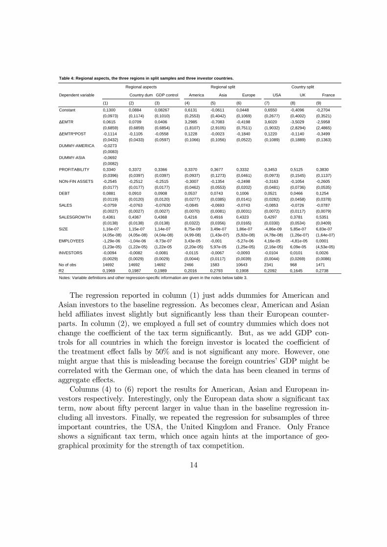
Table 4: Regional aspects, the three regions in split samples and three investor countries.

Dependent variable Country dum GDP control America Asia Europe USA UK France

(1) (2) (3) (4) (5) (6) (7) (8) (9)

Constant 0,1300 0,0884 0,08267 0,6131 ­0,0611 0,0448 0,6550 ­0,4096 ­0,2704(0,0973) (0,1174) (0,1010) (0,2553) (0,4042) (0,1069) (0,2677) (0,4002) (0,3521)

ΔEMTR 0,0615 0,0709 0,0406 3,2985 ­0,7083 ­0,4198 3,6020 ­3,5029 ­2,5958(0,6859) (0,6859) (0,6854) (1,8107) (2,9105) (0,7511) (1,9032) (2,8294) (2,4865)

ΔEMTR*POST ­0,1114 ­0,1105 ­0,0558 0,1228 ­0,0023 ­0,1840 0,1220 ­0,1140 ­0,3499(0,0432) (0,0433) (0,0597) (0,1066) (0,1056) (0,0522) (0,1089) (0,1889) (0,1363)

DUMMY­AMERICA ­0,0273(0,0083)

DUMMY­ASIA ­0,0692(0,0082)

PROFITABILITY 0,3340 0,3372 0,3366 0,3370 0,3677 0,3332 0,3453 0,5125 0,3830(0,0396) (0,0397) (0,0397) (0,0937) (0,1273) (0,0461) (0,0973) (0,1545) (0,1137)

NON­FIN ASSETS ­0,2545 ­0,2512 ­0,2515 ­0,3007 ­0,1354 ­0,2498 ­0,3163 ­0,1054 ­0,2605(0,0177) (0,0177) (0,0177) (0,0462) (0,0553) (0,0202) (0,0481) (0,0736) (0,0535)

DEBT 0,0881 0,0910 0,0908 0,0537 0,0743 0,1006 0,0521 0,0466 0,1254(0,0119) (0,0120) (0,0120) (0,0277) (0,0385) (0,0141) (0,0282) (0,0458) (0,0378)

SALES ­0,0759 ­0,0763 ­0,07630 ­0,0845 ­0,0693 ­0,0743 ­0,0853 ­0,0726 ­0,0787(0,0027) (0,0027) (0,0027) (0,0070) (0,0081) (0,0031) (0,0072) (0,0117) (0,0079)

SALESGROWTH 0,4361 0,4367 0,4368 0,4216 0,4916 0,4323 0,4297 0,3781 0,5351(0,0138) (0,0138) (0,0138) (0,0322) (0,0356) (0,0165) (0,0330) (0,0534) (0,0409)

SIZE 1,16e­07 1,15e­07 1,14e­07 8,75e­09 3,49e­07 1,86e­07 ­4,86e­09 5,85e­07 6,83e­07(4,05e­08) (4,05e­08) (4,04e­08) (4,99­08) (1,43e­07) (5,92e­08) (4,78e­08) (1,26e­07) (1,64e­07)

EMPLOYEES ­1,29e­06 ­1,04e­06 ­9,73e­07 3,43e­05 ­0,001 ­5,27e­06 4,16e­05 ­4,81e­05 0,0001(1,23e­05) (1,22e­05) (1,22e­05 (2,20e­05) 5,97e­05 (1,25e­05) (2,16e­05) 6,09e­05 (4,53e­05)

INVESTORS ­0,0094 ­0,0082 ­0,0081 ­0,0115 ­0,0067 ­0,0093 ­0,0104 0,0101 0,0026(0,0029) (0,0029) (0,0029) (0,0044) (0,0117) (0,0039) (0,0044) (0,0269) (0,0086)

No of obs 14692 14692 14692 2466 1583 10643 2341 968 1471R2 0,1969 0,1987 0,1989 0,2016 0,2793 0,1908 0,2092 0,1645 0,2738

Country splitRegional splitRegional aspects

Notes: Variable definitions and other regression­specific information are given in the notes below table 3.

The regression reported in column (1) just adds dummies for American andAsian investors to the baseline regression. As becomes clear, American and Asianheld a¢ liates invest slightly but signi�cantly less than their European counter-parts. In column (2), we employed a full set of country dummies which does notchange the coe¢ cient of the tax term signi�cantly. But, as we add GDP con-trols for all countries in which the foreign investor is located the coe¢ cient ofthe treatment e¤ect falls by 50% and is not signi�cant any more. However, onemight argue that this is misleading because the foreign countries�GDP might becorrelated with the German one, of which the data has been cleaned in terms ofaggregate e¤ects.Columns (4) to (6) report the results for American, Asian and European in-

vestors respectively. Interestingly, only the European data show a signi�cant taxterm, now about �fty percent larger in value than in the baseline regression in-cluding all investors. Finally, we repeated the regression for subsamples of threeimportant countries, the USA, the United Kingdom and France. Only Franceshows a signi�cant tax term, which once again hints at the importance of geo-graphical proximity for the strength of tax competition.

14

4.3.3 Di¤erent branches

In this subsection we analyse whether �rms in di¤erent branches react di¤erentlyto taxation. Unfortunately we cannot observe branch switchers as do Buch et al.(2005) because the inbound data do not include data on the mother �rms. Table5 reports the regression results for di¤erent branches.

Table 5: Different branches.

Manufacturing Holdings Wholesale Services Finan. serv.

Dependent variable

(1) (2) (3) (4) (5) (6)

Constant 0,0835 0,2402 1,1300 0,1117 0,6792 ­1,3761(0,0976) (0,1615) (0,6742) (0,2003) (0,4201) (1,2535)

ΔEMTR 0,1616 1,0985 8,6646 0,5305 3,5116 ­11,2989(0,7020) (1,1271) (4,8284) (1,4351) (2,9725) (9,0292)

ΔEMTR*POST ­0,1313 ­0,2227 ­1,0407 ­0,0623 ­0,0623 0,6338(0,0432) (0,0658) (0,3935) (0,0590) (0,0590) (0,5886)

BRANCH DUMMIES Yes

PROFITABILITY 0,3278 0,1883 0,9576 0,3309 0,3309 ­0,0880(0,0395) (0,0600) (0,2998) (0,0541) (0,0541) (0,4736)

NON­FIN ASSETS ­0,1915 ­0,2040 0,2633 ­0,1502 ­0,1502 0,0934(0,0181) (0,0268) (0,2071) (0,0319) (0,0319) (0,2680)

DEBT 0,0928 0,0694 0,3031 0,1179 0,1179 0,3076(0,0121) (0,0194) (0,0819) (0,0175) (0,0175) (0,1162)

SALES ­0,0689 ­0,0830 ­0,1671 ­0,0646 ­0,0646 ­0,1047(0,0027) (0,0059) (0,0324) (0,0034) (0,0034) (0,0434)

SALESGROWTH 0,4434 0,5606 ­0,1203 0,5350 0,5350 0,2092(0,0137) (0,0259) (0,0562) (0,0200) (0,0200) (0,1140)

SIZE 7,46e­08 2,04e­07 1,29e­07 2,82e­07 2,82e­07 ­2,47e­08(3,85e­08) (7,87e­08) (6,63e­08) (1,44e­07) (1,44e­07) (6,25e­08)

EMPLOYEES 1,72e­05 ­2,13e­05 2,28e­05 3,21e­05 3,21e­05 0,0002(1,22e­05) (1,80e­05) (0,0003) (4,91e­05) (4,91e­05) (0,0004)

INVESTORS ­0,0084 ­0,0059 ­0,0066 ­0,0064 ­0,0064 ­0,1043(0,0028) (0,0033) (0,0488) (0,0067) (0,0067) (0,0967)

No of obs 14692 4681 530 6215 701 176R2 0,2005 0,2939 0,0838 0,2688 0,1602 0,1331Note: The difference of the sum of observations in columns (2) to (6) is a residual activity group labeled "Others". The 'Services' are specified as'company­related services'. 'Finan. serv.' is financial services.

Including branch dummies increases the �t of the baseline regression, and thetreatment e¤ect is slightly larger. In the manufacturing branch, the coe¢ cient isnearly twice as large as in the baseline regression (without branch dummies). TheR2 is considerably increased. The treatment e¤ects for holdings is nearly ten timeshigher than the one of the total sample. But, the standard error is larger, too, andthe subsample of holdings is relatively small. Interestingly, �rms in the wholesaletrade branch do not show a signi�cant tax treatment term. This is what we expectif wholesale traders are complements to production units elsewhere. The same istrue for services and �nancial services.

15

4.3.4 Quartile analysis

In the following, we analyze both the lowest and the highest quartiles of the sampleaccording to four variables: pro�tability, level of debt, the fraction of non-�nancialassets and the size in terms of balance sheet capital. We do so in order to checkdi¤erent predictions derived from standard tax theory.

Table 6: Highest and lowest quartiles.

Dependent variable lowest highest lowest highest lowest highest lowest highest

(1) (2) (3) (4) (5) (6) (7) (8)

Constant 0,4162 ­0,0590 0,2606 0,3067 0,2274 0,0566 ­0,3119 0,1898(0,1393) (0,1649) (0,1373) (0,1571) (0,2544) (0,0703) (0,1252) (0,1554)

ΔEMTR 1,8694 ­1,3042 1,4189 ­1,0946 1,1530 ­0,2317 ­1,5564 0,2640(0,9762) (1,1780) (0,9811) (1,0536) (1,8246) (0,4927) (0,8784) (1,0944)

ΔEMTR*POST 0,3061 ­0,0950 ­0,2763 ­0,1363 ­0,1822 ­0,1421 0,2407 ­0,1418(0,0973) (0,0794) (0,0849) (0,1031) (0,1338) (0,0459) (0,0843) (0,1005)

PROFITABILITY 0,3061 0,0965 0,3282 0,2570 0,6647 0,2343 0,3780 0,4826(0,0668) (0,0694) (0,0656) (0,0811) (0,1136) (0,0385) (0,0595) (0,0988)

NON­FIN ASSETS ­0,2719 ­0,2355 ­0,1952 ­0,2240 ­7,8412 ­0,1850 ­0,1772 ­0,2718(0,0303) (0,0296) (0,0290) (0,0328) (2,2407) (0,0165) (0,0273) (0,0346)

DEBT 0,0133 0,0971 0,0830 ­0,2626 0,1736 0,0541 0,0910 0,1483(0,0205) (0,0219) (0,0565) (0,0533) (0,0305) (0,0117) (0,0187) (0,0266)

SALES ­0,0760 ­0,0745 ­0,0700 ­0,0768 ­0,0681 ­0,0695 ­0,0573 ­0,0958(0,0054) (0,0046) (0,0052) (0,0053) (0,0064) (0,0028) (0,0044) (0,0061)

SALESGROWTH 0,3989 0,5159 0,3974 0,4259 0,2569 0,5110 0,4157 0,4283(0,0164) (0,0167) (0,0163) (0,0174) (0,0215) (0,0094) (0,0151) (0,0183)

SIZE 1,22e­07 1,31e­07 1,25e­08 7,07e­08 9,83e­08 9,53e­08 3,44e­05 7,62e­08(4,04e­08) (6,94e­08) (2,88e­08) (4,94e­08) (3,35e­08) (3.06e­08) (5,13e­06) (2,32e­08)

EMPLOYEES 3,93e­05 1,4e­05 3,62e­05 ­4,94e­05 0,0002 ­1,19e­06 0,0002 ­8,95e­06(3,08e­05) (2,02e­05) (1,7e­05) (3,46e­05) (0,0001) (1,07e­05) (0,0001) (1,17e­05)

INVESTORS ­0,0027 ­0,0073 ­0,0118 ­0,0048 ­0,0057 ­0,0079 0,0052 ­0,0174(0,0123) (0,0060) (0,0066) (0,0123) (0,0193) (0,0040) (0,0099) (0,0068)

No of obs 3536 3804 3549 3431 3522 3840 3493 3454R2 0,1874 0,233 0,1757 0,1966 0,1009 0,2452 0,2312 0,1879

Note: Profitablity is the average pre­reform ratio of profits over total assets. The level of debt is debt finance over total assets, non­financial assets arealso divided through total assets. The size is equal to total balance sheet assets. Differences in the number of observations are due to rounding errors.

Profitability Level of debt Non­financial assets Size

To begin with pro�tability it is not surprising that the quartile with the lowestpro�tability (which is beyond zero) in column (1) does not show the expected sign.But, as column (2) shows that the �rms in the highest pro�tability quartile do nothave a signi�cant tax treatment e¤ect, either. This could be due to the fact thathighly pro�table �rms do react more strongly to tax rate cuts than to variationsin the marginal tax burden. But this conclusion would require more testing.Columns (3) and (4) show the regression results for the lowest and the highest

quartiles of debt. As predicted by theory, �rms with a low debt level react stronglyto the variation in the e¤ective marginal tax rate, whereas �rms with high debtlevels - i.e. with already high tax shields - do not react signi�cantly.In columns (5) and (6) the lowest and the highest quartiles of non-�nancial

assets are analyzed. The results show that �rms with a high fraction of non-�nancial assets react signi�cantly to the tax reform while �rms with a low fraction

16

do not. We could have expected to �nd more pronounced reactions for �rms withhigh fractions of �nancial assets because the tax-exemption for divestment pro�tsis supposed to be more important for those �rms. However, the results do notcon�rm such a view.The last two columns report the results for the lowest and the highest size

quartiles. The smallest �rms have a wrong sign in the tax treatment e¤ect, thelargest �rms have virtually the same coe¢ cient as in the baseline regression, butit is only marginally signi�cant.

5 Conclusions

In this paper we evaluated the German tax reform of 2000 with respect to itse¤ect on inward foreign direct investment. We solved the identi�cation problemby referring to the rather radical assumption that the aggregate e¤ect of the taxreform is equal to zero. Nevertheless, we found signi�cant tax e¤ects. The baselineregression indicates that a reduction in the e¤ective marginal tax rate increasesnet investment by 1 percentage point. Given an investment level of around 0,1and an EMTR of around 0,4, the elasticity of investment with respect to e¤ectivemarginal taxation is approximately equal to 0,4. In comparison to other empiricalstudies this estimate is rather at the bottom line, but it should be recalled againthat our results are based on an assumed aggregate e¤ect of zero.

References

Becker, J., Fuest, C. & Hemmelgarn, T. (2005). The impact of business taxationon FDI �ows in Europe-a critical review of existing studies and new evidence,mimeo.

Bénassy-Quéré, A., Fontagné, L. & Lahrèche-Révil, A. (2005). How Does FDIReact to Corporate Taxation?, International Tax and Public Finance 12(5): 583�603.

Bertrand, M., Du�o, E. & Mullainathan, S. (2004). How much should wetrust di¤erences-in-di¤erences estimates?, Quarterly Journal of Economics119(1): 249�275.

Buch, C. M., Kleinert, J., Lipponer, A. & Toubal, F. (2005). Determinants and Ef-fects of Foreign Direct Investment: Evidence from German Firm-Level Data,Economic Policy 0(41): 51�98.

17

Büttner, T. & Ruf, M. (2004). Tax Incentives and the Location of FDI: Evidencefrom a Panel of German Multinationals, ZEW Discussion Paper (04-76).

Cummins, J. G., Hassett, K. A. & Hubbard, R. G. (1994). A Reconsideration ofInvestment Behavior Using Tax Reforms as Natural Experiments, BrookingsPapers on Economic Activity (2): 1�59, 70�74.

Devereux, M. P. & Gri¢ th, R. (1998). Taxes and the location of production:Evidence from a panel of US multinationals, Journal of Public Economics(68) 3: 335�367.

Fuest, C., Huber, B. & Mintz, J. (2005). Capital Mobility and Tax Competition,Foundations and Trends in Microeconomics .

Hanlon, M., Mills, L. & Slemrod, J. (2005). An empirical examination of cor-porate tax noncompliance, University of California. Paper presented at theconference on "Taxing corporate income in the 21st century".

Hines, J. R. (1999). Lessons from behavioral responses to international taxation,National Tax Journal 52(2): 305�322.

Homburg, S. (2000). German Tax Reform 2000: Description and Appraisal, Fin-anzArchiv 57(4): 504�513.

Keen, M. (2002). The German Tax Reform of 2000, International Tax and PublicFinance 9(5): 603�621.

Lipponer, A. (2003). Deutsche bundesbank�s FDI micro database, SchmollersJahrbuch - Zeitschrift für Wirtschafts- und Sozialwissenschaften. 123: 593�600.

Markusen, J. R. (2002). Multinational Firms and the Theory of InternationalTrade, Massachussets Institute of Technology, Cambridge, USA.

Mooij de, R. A. & Ederveen, S. (2003). Taxation and foreign direct investment: Asynthesis of empirical research, International Tax and Public Finance 10: 673�693.

Schreiber, U. (2000). German Tax Reform - An International Perspective, Finan-zArchiv 57(4): 525�541.

Slemrod, J., Dauchy, E. & Martinez, C. (2005). Corporate tax avoidance and thee¤ectiveness of tax incentives for investment, University of Michigan, mimeo.

18

Spengel, C. (2001). Der Steuerstandort Deutschland im Internationalen Ver-gleich, Eine Analyse Vor Dem Hintergrund Des Steuersenkungsgesetzes2001, Expertise Für Den Sachverständigenrat Zur Begutachtung der Ges-amtwirtschaftlichen Entwicklung, Universität Mannheim.

Wilson, J. D. & Wildasin, D. E. (2004). Capital Tax Competition: Bane or Boon,Journal of Public Economics, Special Issue 88(6): 1065�91.

19