corporate bond valuation - faculty.baruch.cuny.edu

Corporate bond valuation

Liuren Wu

2021

c©Liuren Wu (Baruch) Corporate bond 2021 1 / 27

Pricing defaultable bonds with DTSM

For a default-free zero-coupon bond, the terminal payoff is certain atΠT = 1. The valuation is

B(t,T ) = Et [Mt,T ] = EQt

[exp

(−∫ T

t

rsds

)].

If the bond can default, Duffie and Singleton (1999) show that for pricingpurposes, one can replace the discount rate rt with the “default-adjusted”rate rt + htLt , where h is the risk-neutral intensity of default and L isrisk-neutral expected fractional loss in market value in the event of default.

When it is difficult to distinguish the two components ht and Lt , onecan directly model the “instantaneous spread” st = htLt .Liquidity effects can be analogously captured by an instantaneousspread (Duffie, Pedersen, and Singleton (2003)).One can also directly model a default and liquidity-adjusted short ratert .How one should decompose the discount rate is mainly driven byidentification and the question one wants to address.


Examples

1 If one wants to model the interaction between on-the-run and off-the-runTreasuries, one can start with a shortt rate r for on-the-run bonds, and addan instantaneous spread st for off-the-run bonds.

2 Corporate bond pricing:

One normally uses the on-the-run Treasury to define benchmark “riskfree” rate curve, even though nowadays Treasuries are no longerregarded as risk free.The effects of credit (and other) risks in a corporate bond can becaptured by an instantaneous spread on top of the Treasury curve.

3 Pricing equity options, credit default swap (CDS) spreads ...

Traditionally researchers use the Treasury rates to define the “riskfree”curve for option pricing, now most (including OptionMetrics) hasswitched to the underlying LIBOR/swap curve, which is not risk free.For CDS and other credit risk modeling, the instantaneous credit (andliquidity) spread st is also defined on top of the LIBOR/swap curve.Instead of calling rt the risk free rate, I often refer to it as the”benchmark” rate.


Pricing CDS as an example

A CDS is an OTC contract between the seller and the buyer of protectionagainst the risk of default on a set of debt obligations issued by a referenceentity.

It is essentially an insurance policy that protects the buyer against the lossof principal on a bond in case of a default by the issuer.

The protection buyer pays a periodic premium over the life of the contractand is, in turn, covered for the period.

The premium paid by the protection buyer to the seller is often termed asthe “CDS spread” and is quoted in basis points per annum of the contract’snotional value and is usually paid quarterly.

If a certain pre-specified credit event occurs, the premium payment stopsand the protection seller pays the buyer the par value for the bond.

If no credit event occurs during the term of the swap, the protection buyercontinues to pay the premium until maturity.

The contract started in the sovereign market in mid 90s, but the volume hasmoved to corporate entities.


Credit events

A CDS is triggered if, during the term of protection, an event that materiallyaffects the cashflows of the reference debt obligation takes place.

A credit event can be a bankruptcy of the reference entity, or a default of abond or other debt issued by the reference entity.

Restructuring is considered a credit event for some, but not all, CDScontracts, referred to as “R”, “mod-R”, or “modmod- R”. Events such asprincipal/interest rate reduction/deferral and changes in priority ranking,currency, or composition of payment can qualify as credit events.

When a credit event triggers the CDS, the contract is settled andterminated. The settlement can be physical or cash. The protection buyerhas a right to deliver any deliverable debt obligation of the reference entityto the protection seller in exchange for par.

There can be additional maturity restrictions if the triggering credit event isa restructuring.

The CDS buyer and the seller can also agree to cash settle the contract atthe time of inception or exercise. In this case, the protection seller pays anamount equal to par less the market value of a deliverable obligation.

It is this probability weighted expected loss that the CDS premium strives tocapture.c©Liuren Wu (Baruch) Corporate bond 2021 5 / 27

Standardized payment dates

Since 2002, a vast majority of CDS contracts have standardized quarterlypayment and maturity dates — 20th of March, June, September, andDecember.

This standardization has several benefits including convenience in offsettingCDS trades, rolling over of contracts, relative value trading, single name vs.the benchmark indices or tranched index products trading.

After the 2008 financial crises, there is a strong movement toward centralclearing and more standardization:

The CDS spread is standardized to either 100 and 500 basis points.The value of the contract is settled with upfront payment.


CDS pricing

The fair CDS spread (premium) is set to equate the present value of allpremium payments to the present value of the expected default loss, both inrisk-adjusted sense.

There is typically an accrued premium when default does not happen exactlyon the quarterly payment dates.

Consider a one period toy example, in which the premium (s) is paid at theend of the period and default can only happen at the end of the period withrisk-adjusted probability p. In case of default, the bond’s recovery rate is R.

The present value of the premium payment is: N(1− p)s/(1 + r).The present value of the expected default loss: Np(1− R)/(1 + r).

Equating the values of the two legs, we have s = p(1−R)(1−p) ≈ p(1− R).

Or from a CDS quote s, we can learn the risk-adjusted defaultprobability as p = s

s+1−R ≈s

1−R .


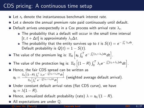
CDS pricing: A continuous time setup

Let rt denote the instantaneous benchmark interest rate.

Let s denote the annual premium rate paid continuously until default.

Default arrives unexpectedly in a Cox process with arrival rate λt .

The probability that a default will occur in the small time interval[t, t + ∆t] is approximately λt∆t.

The probability that the entity survives up to t is S(t) = e−∫ t0λsds .

Default probability is Q(t) = 1− S(t).

The value of the premium leg is: E0

[s0∫ T

0e−

∫ t0(rs+λs )dsdt

].

The value of the protection leg is: E0

[(1− R)

∫ T

0λte−

∫ t0(rs+λs )dsdt

].

Hence, the fair CDS spread can be written as

s0 =E0

[(1−R)

∫ T0λte

−∫ t0 (rs+λs )dsdt

]E0

[∫ T0

e−∫ t0(rs+λs )dsdt

] (weighted average default arrival).

Under constant default arrival rates (flat CDS curve), we haves0 = λ(1− R).

Hence, annualized default probability (rate) λ = s0/(1− R).

All expectations are under Q.c©Liuren Wu (Baruch) Corporate bond 2021 8 / 27

Interactions between interest rates and credit spreads

If we only need to value the premium leg, we can model the dynamics of thedefaultable rates xt = rt + λt directly.

To value the protection leg (and derive the CDS spread value), we need toseparately model the dynamics of rt and λt ,

Technically, if we model both r and λ as affine functions of some affinefactors Xt , we would have tractable exponential-affine solutions as describedearlier: rt = ar + b>r Xt , λ

it = ai + b>i Xt .

Technically you can add any interactions you want, but practically they mustbe economically sensible and preferably parsimonious.

The benchmark rate r is a market-wide variable, it is appropriate tostart with r and specify how each firm’s credit depends on the market:

rt = ar + b>r Xt ,λit = ai + b>i Xt + c>i Yt

dXt = (θx − κxXt) dt + dWxt ,dYt = (θy − κxyXt − κyYt) dt + dWyt ,

Yt is firm-specific credit risk. Note the two types of interactions(contemporaneous v. predictive).


Summary: Term structure decomposition

Interest rates can be different at different terms (maturities). The patternacross different terms is referred to as the term structure behavior.

Generically speaking, the interest rate term structure can be decomposedinto three components:

1 Expectation: Long-term rates reflect the expectation of futureshort-term rates.

2 Risk premium: Long-term bonds are more sensitive to rate movements(and riskier), and hence higher returns (yields) on average.

3 Convexity: The bond value dependence on rate is convex, more so forlong-term bonds. High rate volatility benefits long bond holders. Assuch, they can afford to ask for a lower expected return (yield).

The decomposition can be most clearly seen from the forward rate relationunder a simplified Vasick model:

drt = σdWt , f (t, τ) = rt − γστ −1

2σ2τ 2

The three-component term structure decomposition works whether the“short rate” r is default-free or default able.


Summary: Short-rate risk decomposition

In many applications, it is useful to decompose the short rate into severalcomponents and model the dynamics of each component separately/jointly.

1 General affine: Short rate is decomposed into a linear combination ofseveral “factors.”

2 Credit risk: The short rate for defaultable bond can be decomposedinto a benchmark component and a credit spread.

The traditional benchmark tends to be a “default-free” rate, now moststudies switch to a practical benchmark actually used in the industry,which is not necessarily default free.

3 Liquidity risk: Liquidity risk can also be separated out as a short ratespread against some more liquid benchmark.

4 Benchmark rate, credit spread, liquidity spread can each be furtherdecomposed, for example, into different frequency components.

The exact decomposition depends on the type of questions one wants toaddress, always with identification in mind.

The technicality (tractability) behind the bond pricing is the same,regardless of the economic meanings of the decomposition.


Capital structure decisions and default probability

In the previous sections, we specify interest and credit risk dynamics andderive interest rate and credit spread term structure.

But what dictates the credit risk (and its dynamics) of a firm?

The starting point must be the company’s capital structure: If a companydoes not have any liability, it has nothing to default on. The larger theliability (the higher the leverage), the more likely the firm can havedifficulties meeting its liability obligations in the future.

Different types of business operations can accommodate different levels ofleverage, for the same degree of risk.

Business risk: If you know how much money you need and you cangenerate at each point in time, you can borrow up to that point, withno chance of default. Otherwise, you need to leave cushions.Refinancing flexibility/risk: If you can borrow new debt (or raise equity)to pay old debt, you don’t need to default, either.Investment flexibility: If you can freely adjust your investment position(asset characteristics), the chance of default is much smaller.

Capital structure is not (always) a static feature of a firm, but adecision/control variable that the managers can actively work on/adjust.


The Merton (1974) model: Set up

Assumptions:

The company has a zero-coupon bond with principal D and expiring atT . Company defaults if and only if its asset value at time T , AT is lessthan the debt principal.Asset values follows a geometric Brownian motion (GBM):dAt/At = µdt + σAdWt .

Comments:

The company does not have the flexibility of adjusting leverage,refinancing, or changing investments/business.The model captures two key elements of default risk: leverage andbusiness risk, in a very simple and intuitive way.

Models that start with the capital structure description and asset valuedynamics are often referred to as “structural models,” in contrast with“reduced-form” models that directly specify default arrival rate dynamics.

Each type of model serves a different purpose ...


The Merton (1974) model: Pricing

Under Merton (1974), equity is a European call option on the asset: At debtmaturity T , the equity holders receive (AT − D)+.

Under the GBM dynamics, the call-option (equity) value satisfies theBlack-Merton-Scholes formula: Et = AtN(d + σA

√τ)− DN(d),

where d is a standardized variable that measures the number of standarddeviations by which the log debt principal is below the conditionalrisk-neutral mean of the log asset value,

d =EQt (lnAT )− ln(D)

Stdt(lnAT )=

ln(At) + rτ − 12σ

2Aτ − ln(D)

σA√τ

.

In the option pricing literature, d is referred to as the standardizedmoneyness of the option.In the structural model literature, d is referred to as thedistance-to-default, a critical input for Moody’s credit model.The numerator measures the expected financial leverage of the firm atthe debt expiration, and the denominator measures the uncertainty(standard deviation) of this leverage — Distance to default isessentially a standardized financial leverage measure that is comparableacross firms with different business risks.


The Merton (1974) model: Key contribution

The key contribution of the model is the distance to default measure, whichstandardizes the capital structure (financial leverage) to make it comparableacross firms with different business risk profiles.

Broadly speaking, a firm’s (or a person’s) credit is determined by bothwhat it has (balance sheet) and what it is going to make (incomestatement)The distance-to-default measure captures mainly what a firm has;traditional credit measures such as interest coverage ratio mainlycapture the firm’s earning power.One can modify the distance to default to capture both, by replacingrisk-neutral return r with actual RoA forecasts.

Another key advantage of the model is that it links the valuation of equitywith the valuation of bond via the firm value dynamics

The model allows one to predict cross-sectional variation of corporatebond credit spreads (or CDS spreads) with firm characteristics (Bai &Wu, 2016).One can also use the model to perform capital structure arbitragetrading: stock options/stock v. bond.


Beyond Merton: Limitations and extensions

The key characteristics of a great model is that it makes bold/dramaticsimplifying assumptions to arrive at deep insights that make economic sense.

One key objective of “structural” credit modeling is to see through themillions of details in a firm and show how different firm characteristicscombine to determine credit risk.

The Merton model says that the key credit determinants are financialleverage and business risk and their contributions do not come inadditively, but one serves as a scaler of the other.

Given the highly stylized nature, the model can of course be extended inseveral dimensions:

1 Asset value dynamics2 Capital structure specifications3 Default triggering mechanisms4 Firm operation, investment, and refinancing decisions


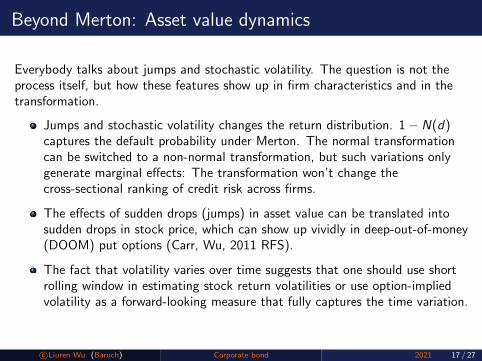
Beyond Merton: Asset value dynamics

Everybody talks about jumps and stochastic volatility. The question is not theprocess itself, but how these features show up in firm characteristics and in thetransformation.

Jumps and stochastic volatility changes the return distribution. 1− N(d)captures the default probability under Merton. The normal transformationcan be switched to a non-normal transformation, but such variations onlygenerate marginal effects: The transformation won’t change thecross-sectional ranking of credit risk across firms.

The effects of sudden drops (jumps) in asset value can be translated intosudden drops in stock price, which can show up vividly in deep-out-of-money(DOOM) put options (Carr, Wu, 2011 RFS).

The fact that volatility varies over time suggests that one should use shortrolling window in estimating stock return volatilities or use option-impliedvolatility as a forward-looking measure that fully captures the time variation.


Beyond Merton: Capital structure specification

Virtually all firms have debt of multiple maturities, including coupon/interestexpense payments in the middle.

Even if one uses the Merton model, how to implement the model remains anissue. For example, KMV uses short-term liability + half of long-termliability to proxy the debt principal D in Merton model. Why?

Given the same amount of total debt, which types of firms have highercredit risk at different horizons? Firms with more short-term or morelong-term debt?

These questions cannot be appropriately addressed theoretically withoutmaking the right assumption on the default triggering mechanism, whichmay also depend on the (flexibility) of the refinancing decision.

Do firms only default at debt payment period or can they default atany time? Can debt holders force bankruptcy preemptively?When one debt matures, should/will the firm pay off the debt with itscurrent earnings (by paying less dividend), its asset (via liquidation), orrefinancing (via equity or debt)?


Beyond Merton: Debt payment decisions

If the firm plans to payoff its obligation using earnings, it better has enoughearnings to cover the payment — Interest coverage ratio relies on this idea.

If the firm plans to liquidate asset to cover its debt payment, its asset musthave a significant component that can be liquidated easily — liquidity ratiosare useful indicators.

Investment firms can reduce their investment size fairly easily and theyindeed do so frequently according to market conditions; but it can becostly for a manufacturing firm to do so.

If the firm plans to refinance its expiring debt, market credit conditions canbecome an important concern. Also, all variables that are considered by debtinvestors (profitability, existing leverage, liquidity, size, past performance,etc) become naturally important in determining the refinancing cost (andpossibility).

There are many structural models that go beyond Merton, such as Leland,Geske, etc. You can also try to think of new models. Practically, the key iswhether these extensions allow you to incorporate more useful informationobserved on the firm.


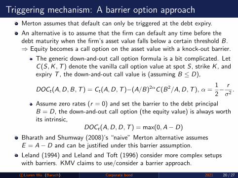
Triggering mechanism: A barrier option approach

Merton assumes that default can only be triggered at the debt expiry.

An alternative is to assume that the firm can default any time before thedebt maturity when the firm’s asset value falls below a certain threshold B.⇒ Equity becomes a call option on the asset value with a knock-out barrier.

The generic down-and-out call option formula is a bit complicated. LetC (S ,K ,T ) denote the vanilla call option value at spot S , strike K , andexpiry T , the down-and-out call value is (assuming B ≤ D),

DOCt(A,D,B,T ) = Ct(A,D,T )−(A/B)2αC (B2/A,D,T ), α =1

2− r

σ2.

Assume zero rates (r = 0) and set the barrier to the debt principalB = D, the down-and-out call option (the equity value) is always worthits intrinsic,

DOCt(A,D,D,T ) = max(0,A− D)

Bharath and Shumway (2008)’s “naive” Merton alternative assumesE = A− D and can be justified under this barrier assumption.

Leland (1994) and Leland and Toft (1996) consider more complex setupswith barriers. KMV claims to use/consider a barrier approach.


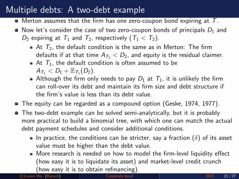
Multiple debts: A two-debt exampleMerton assumes that the firm has one zero-coupon bond expiring at T .

Now let’s consider the case of two zero-coupon bonds of principals D1 andD2 expiring at T1 and T2, respectively (T1 < T2).

At T2, the default condition is the same as in Merton: The firmdefaults if at that time AT2 < D2, and equity is the residual claimer.At T1, the default condition is often assumed to beAT1 < D1 + ET1(D2).Although the firm only needs to pay D1 at T1, it is unlikely the firmcan roll-over its debt and maintain its firm size and debt structure ifthe firm’s value is less than its debt value.

The equity can be regarded as a compound option (Geske, 1974, 1977).

The two-debt example can be solved semi-analytically, but it is probablymore practical to build a binomial tree, with which one can match the actualdebt payment schedules and consider additional conditions.

In practice, the conditions can be stricter, say a fraction (δ) of its assetvalue must be higher than the debt value.More research is needed on how to model the firm-level liquidity effect(how easy it is to liquidate its asset) and market-level credit crunch(how easy it is to obtain refinancing).


Free of default via flexible leverage rebalancing

Merton and Geske assume that default only occur at debt payment times.

These companies have a passive debt structure that will only beupdated upon debt expiry.

Financial firms, including banks and investment firms, can be much moreactive in rebalancing their financial leverage (Adrian and Shin (2010)).

Think of the simplest example of trading on margin.

Trading on margin is essentially levered investment. The asset is theamount of the investment, which can be several times higher than theequity (the amount of margin one puts at the exchange).One rarely observes default on margin trading, despite high leverage.The key is that it has a barrier feature at which point the creditor(exchange) can force close the position if no new capital is injected.The barrier is set at a level that the creditor rarely loses money at theforced closure.The debt can be thought of as short-term credit.

If asset follows diffusion dynamics and the firm can flexibly (and optimally)adjust the financial leverage, the firm in principal never needs to default.Investment flexibility can play a similar role.c©Liuren Wu (Baruch) Corporate bond 2021 22 / 27

Constant proportional portfolio insurance (CPPI)

This may be a side topic, but it is somewhat useful in terms of how we think ofcredit risk, especially for financial firms.

CPPI allows an investor to limit downside risk while retaining some upsidepotential by maintaining an exposure to risky assets equal to a constantmultiple m > 1 of the cushion. In diffusion models with continuous trading,this strategy has no downside risk.

CPPI is a self-financing strategy, with the goal to guarantee a fixed amountN of capital at maturity T .

Let Bt denote the present value of the guaranteed amount N and Vt denotethe total portfolio value. The strategy at any date t can be described as,

If Vt > Bt , the risky asset exposure (amount of money invested intothe risky asset) is given by mCt = m(Vt − Bt), where Ct is the“cushion” and m > 1 is a constant multiplier.If Vt ≤ Bt , the entire portfolio is invested into the zero-coupon.

If one can guarantee a fixed amount at expiration, one never needs todefault.


Diffusion risk does not cause default, jumps do

Under the Merton model, the diffusion nature of the dynamics dictates thatthe default event is completely predictable before it happens.

We show via the CPPI strategy that one can always avoid the predictableevent if one is allowed to scale the risky investment freely.

Hence, the true risk under the Merton model is not from the diffusiondynamics, but from structural constraints — the firm cannot do anything toget out once in the debt.

However, when the asset value can jump down unexpectedly by a largeamount, even frequent rebalancing cannot guarantee default free.

Actions no longer help, it is fate.

Thus, in practice, one should be worried (or not) about large downsidejumps, while working actively to avoid difficulties caused by diffusionmovements (via active rebalancing).


DOOM puts as credit insurance

Carr and Wu (2011,RFS) assume that the stock price stays above B beforedefault and falls 0 after default.

There is a default corridor [0,B] that the stock price can never reside in.

This can happen if asset value dynamics can jump through a corridorthat brackets the default trigger...The corridor effect dominates the capital structure variation.

In the presence of the default corridor, one can use a deep-out-of-money(DOOM) American put stock option struck within the corridor to create apure credit contract

URC = P(K ,T )/K (with K ≤ B) denotes a unit recovery claim thatpays one dollar when and only when the firm defaults!If the corridor has a non-zero lower bound (non-zero equity recovery),we can choose two put options struck within the corridor to create theunit recovery claim, URC = (P(K2)− P(K1))/(K2 − K1).

The URC implications hold, regardless of pre-default or post-defaultdynamics... It only depends on the presence of a default corridor.

Cross-market arbitrage between DOOM puts and credit insurance


Two types of defaults

Fundamentally, there are two types of defaults that ask for different types ofresponses and have different levels of market impacts.

1 Structural defaults: Defaults due to structural constraints.

Both creditors and debtors can see default coming, but they arestructurally constrained to do anything about it.The Merton (1974) model is one such case: The diffusion behaviordictates that default event is predictable, yet creditors are not allowedto force close the debt early to avoid loss of principal.The barrier option alternative assumption allows the creditor to get outearly as soon as the asset value hits a boundary. Under certainassumptions, the creditor never loses its principal.The CPPI example is inspirational in the sense that the financialmanagers can drastically reduce their chance of default (to zero) underdiffusion dynamics if they can actively rebalance theirportfolio/leverage — All firms have some capacity to do so, more forfinancial firms (such as investment banks) and investment firms.

To avoid defaults caused by structural constraints, financial managers shouldstrive to keep credit channels open, maintain a flexible capital structure thatcan be readily updated/adjusted based on market conditions...c©Liuren Wu (Baruch) Corporate bond 2021 26 / 27

Two types of defaults

Fundamentally, there are two types of defaults that ask for different types ofresponses and have different levels of market impacts.

1 Defaults induced by structural constraints

2 Default induced by exogenous sudden, large, market shocks:

It is difficult to neutralize such shocks via dynamic hedging, whichworks better for diffusions or jumps of fixed/known sizes than forjumps of random sizes.One can in principle take (many) option positions to hedge jumps ofdifferent sizes — The strong aggregate demand for such insurance-likeoption contracts often pushes the option price to very high levels.Worse yet, large negative shocks often generate chain reactions, or“self-exciting behavior:” One large negative shock tends to increase thechance of having more large negative shocks to follow, eithersequentially for one firm or one market (destabilizing spiral), orcross-sectionally across different firms or markets (contagion).

World-wide crash-o-phobia (Foresi & Wu, 2005, Wu, 2006): Deepout-of-money put options are very expensive on market indexes across theworld, more so for longer-term options.


corporate bond valuation - faculty.baruch.cuny.edu

Documents