core.ac.uk · modelizaci on, ecuaciones diferenciales. contents 1 introduction13 ... (ode). it has...
TRANSCRIPT

Title: A logistic queue model for network traffic modeling and simulation
Author: Franco Coltraro Ianniello
Advisor: Luis Velasco Esteban
Co-Advisor: Marc Ruiz Ramírez
Department: Computers Architecture
Academic year: 2016-2017
Master of Science in Advanced Mathematics andMathematical Engineering


Agradecimientos
Me gustarıa agredecer a mis tutores Luis Velasco y Marc Ruiz y en general a todo el Grupode Comunicaciones Opticas por haberme dado la excelente oportunidad de trabajar un anoentero en un ambiente de investigacion emocionante y estimulante. Agradezco tanto el apoyoacademico y personal que el grupo me ha brindado, como el economico.
Tampoco puedo dejar de agradecer a mis amigos de Madrid y Barcelona el haberme aguan-tado un ano entero diciendo que mi cola era la mejor del mundo. Finalmente, me gustarıarecordar el apoyo incondicional de mis padres y mi hermano.


Abstract
In this work we present a continuous queuing model called the logistic queue model.We show that in terms of queue size and outflow prediction, our model is as precise as adiscrete event simulator with the additional advantage of speed in simulations. We provemathematically that our proposed model has all the theoretical properties one should expect,e.g. positivity of queue, FIFO property. Finally, in contrast with other continuous models–Vickrey’s point-queue model– our model can be easily integrated numerically and moreoverit allow us to naturally explore multiple extensions relevant to telecommunication networkssuch as: finite queues, multiple servers, priority queues, etc.
Keywords: queueing theory, fluid flow model, fluid queues, telecommunication networks,simulation, modeling, differential equations.
Resumen
En este trabajo presentamos un modelo continuo de teorıa de colas llamado el modelode la cola logıstica. Mostramos que en cuanto al tamano de la cola y a la prediccion delfujo de salida se refiere, este es tan preciso como un simulador de eventos discretos conla ventaja de ser mas rapido en las simulaciones. Demostramos matematicamente que elmodelo posee propiedades teoricas importantes, e.g. positividad de la cola, propiedad FIFO.Asimismo, a diferencia de otros modelos continuos –modelo de la cola puntual de Vickrey–nuestro modelo puede integrarse numericamente con facilidad y ademas puede extendersepara casos relevantes a las redes de telecomunicaciones: colas finitas, colas con prioridades,etc.
Palabras clave: teorıa de colas, colas fluidas, redes de telecomunicaciones, simulacion,modelizacion, ecuaciones diferenciales.

Contents
1 Introduction 13
1.1 Motivation . . . . . . . . . . . . . . . . . . . . . . . . . . . . . . . . . . . . . 13
1.2 Contributions . . . . . . . . . . . . . . . . . . . . . . . . . . . . . . . . . . . 15
1.3 Organization . . . . . . . . . . . . . . . . . . . . . . . . . . . . . . . . . . . 15
2 Background 17
2.1 Introduction to dynamic optical networks . . . . . . . . . . . . . . . . . . . . 17
2.2 Queuing models . . . . . . . . . . . . . . . . . . . . . . . . . . . . . . . . . . 19
2.3 Summary . . . . . . . . . . . . . . . . . . . . . . . . . . . . . . . . . . . . . 21
3 The logistic queue model 23
3.1 Derivation . . . . . . . . . . . . . . . . . . . . . . . . . . . . . . . . . . . . . 23
3.2 Theoretical Properties . . . . . . . . . . . . . . . . . . . . . . . . . . . . . . 26
3.3 Applying the model . . . . . . . . . . . . . . . . . . . . . . . . . . . . . . . . 32
3.3.1 Discrete inflow . . . . . . . . . . . . . . . . . . . . . . . . . . . . . . 32
3.3.2 Integrating the ODE . . . . . . . . . . . . . . . . . . . . . . . . . . . 32
3.3.3 Queue error due to aggregation time . . . . . . . . . . . . . . . . . . 32
3.4 Summary . . . . . . . . . . . . . . . . . . . . . . . . . . . . . . . . . . . . . 33
4 Extensions for Communication Networks 35
4.1 Variable service times . . . . . . . . . . . . . . . . . . . . . . . . . . . . . . . 35
4.2 Finite queue . . . . . . . . . . . . . . . . . . . . . . . . . . . . . . . . . . . . 35
4.3 Multiple servers . . . . . . . . . . . . . . . . . . . . . . . . . . . . . . . . . . 38
7
8 CONTENTS
4.4 Separation of flows . . . . . . . . . . . . . . . . . . . . . . . . . . . . . . . . 38
4.5 Priority queues . . . . . . . . . . . . . . . . . . . . . . . . . . . . . . . . . . 39
4.6 Summary . . . . . . . . . . . . . . . . . . . . . . . . . . . . . . . . . . . . . 39
5 Validation and Results 41
5.1 Notations . . . . . . . . . . . . . . . . . . . . . . . . . . . . . . . . . . . . . 41
5.2 Error measures . . . . . . . . . . . . . . . . . . . . . . . . . . . . . . . . . . 42
5.3 User service characterization . . . . . . . . . . . . . . . . . . . . . . . . . . . 42
5.4 Implementation . . . . . . . . . . . . . . . . . . . . . . . . . . . . . . . . . . 45
5.5 Illustrative example . . . . . . . . . . . . . . . . . . . . . . . . . . . . . . . . 46
5.6 Performance Analysis . . . . . . . . . . . . . . . . . . . . . . . . . . . . . . . 50
5.7 Summary . . . . . . . . . . . . . . . . . . . . . . . . . . . . . . . . . . . . . 55
6 Case study example 57
6.1 Scenario . . . . . . . . . . . . . . . . . . . . . . . . . . . . . . . . . . . . . . 57
6.2 Applying the logistic queue model . . . . . . . . . . . . . . . . . . . . . . . . 59
6.3 Empirical results . . . . . . . . . . . . . . . . . . . . . . . . . . . . . . . . . 60
6.4 Summary . . . . . . . . . . . . . . . . . . . . . . . . . . . . . . . . . . . . . 61
7 Concluding Remarks 63
7.1 Contributions archieved . . . . . . . . . . . . . . . . . . . . . . . . . . . . . 63
7.2 Personal evaluation . . . . . . . . . . . . . . . . . . . . . . . . . . . . . . . . 63
7.3 Future work . . . . . . . . . . . . . . . . . . . . . . . . . . . . . . . . . . . . 64
Bibliography 65
List of Figures
2.1 Simplified network architecture example. . . . . . . . . . . . . . . . . . . . 18
2.2 Schematic picture of a system consisting of a server with a queue. . . . . . . 19
2.3 Flow-chart associated to system consisting of a server with a queue. . . . . . 20
3.1 Example of a system with a queue and a server of speed µ. . . . . . . . . . 23
3.2 Possible outflows we may get at a fixed instant of time t0 depending on thequeue size C0. . . . . . . . . . . . . . . . . . . . . . . . . . . . . . . . . . . 25
3.3 C is decreasing in [t+, t−]. . . . . . . . . . . . . . . . . . . . . . . . . . . . . 26
3.4 Plot of queue size (3.11) for constant inflow f(t) ≡ 0.5 with µ = 1, α = 12
andC0 = 1. . . . . . . . . . . . . . . . . . . . . . . . . . . . . . . . . . . . . . . . 29
3.5 Comparison of Tε and Tε for µ = 1, f∞ = 0.5, α = 12
and ε = 0.05. . . . . . . 30
4.1 Approximations of Heaviside function for k = 5, 10. . . . . . . . . . . . . . . 36
4.2 Two flows join in a server with a queue and then each of them follow a differentpath. . . . . . . . . . . . . . . . . . . . . . . . . . . . . . . . . . . . . . . . 38
5.1 Simulation of packets generated by a video user during two hours. Each blueline represents a packet. . . . . . . . . . . . . . . . . . . . . . . . . . . . . . 44
5.2 Flow fv generated by one video user during two hours. . . . . . . . . . . . . 45
5.3 Implementation of a queue with a server in Simulink. . . . . . . . . . . . . . 46
5.4 Inflow to the system. Its standard deviation is 2.53 Mb/s. . . . . . . . . . . 47
5.5 Queue of the discrete simulator. . . . . . . . . . . . . . . . . . . . . . . . . . 48
5.6 Queue of the logistic model. . . . . . . . . . . . . . . . . . . . . . . . . . . . 48
5.7 Superposition of logistic and discrete queues in a neighborhood of the maxi-mum queue occupancy. . . . . . . . . . . . . . . . . . . . . . . . . . . . . . . 49
9

10 LIST OF FIGURES
5.8 Outflow of discrete simulator. . . . . . . . . . . . . . . . . . . . . . . . . . . 49
5.9 Outflow of logistic model. . . . . . . . . . . . . . . . . . . . . . . . . . . . . 49
5.10 Comparison of maximum queue size for both models varying the inflow inten-sity. . . . . . . . . . . . . . . . . . . . . . . . . . . . . . . . . . . . . . . . . 51
5.11 Maximum occupancy error of the logistic model varying the inflow intensity. 52
5.12 Error relative to the maximum of the logistic model varying the inflow intensity. 52
5.13 Global relative error of the outflows given by logistic model and the no-queuemodel varying the inflow intensity. . . . . . . . . . . . . . . . . . . . . . . . . 53
5.14 Mean relative error of the outflows given by logistic model and the no-queuemodel varying the inflow intensity. . . . . . . . . . . . . . . . . . . . . . . . . 54
5.15 Simulation times of logistic and discrete queue model varying the inflow in-tensity. . . . . . . . . . . . . . . . . . . . . . . . . . . . . . . . . . . . . . . . 54
6.1 Network for the scenario in flow form. The goal is to send packets from regiono to region d of the network. In the picture n = 2 and m = 3. . . . . . . . . 58
6.2 Network for the scenario in packet form. The goal is to send packets fromregion o to region d of the network. In the picture n = 2 and m = 3. . . . . 58
6.3 Expected latency in seconds of going from region o to region d. . . . . . . . 61
6.4 Maximum expected latency in seconds of going from region o to region dvarying the intensity of an extra priority flow in the simulation. . . . . . . . 62

List of Tables
5.1 Estimation of parameters for a video user. . . . . . . . . . . . . . . . . . . . 43
5.2 Length of video consumptions and their probabilities. . . . . . . . . . . . . 44
11

12 LIST OF TABLES

Chapter 1
Introduction
1.1 Motivation
The expected explosion of services offered on the Internet has revealed new paradigms intelecommunication networks. Traffic forecasts in [1] and [2] reveal that the exchange of databetween data-centers (DCs) will reach 905 exabytes per year by 2019. This is induced byan increasing IP traffic that will be mainly coped by video services: 80% of total IP traffic by2019. Aiming at interconnecting DCs and services, connectivity from the transport networkis required to carry traffic flows between network nodes, each consisting of a mix of differentservices.
From the network perspective, transport networks are currently configured with bigstatic fat pipes. They are based on capacity over-provisioning aiming at guaranteeing trafficdemand and Quality of Service (QoS). Cloud-ready transport network [3] was introduced asan architecture to handle a dynamic cloud and network interaction. The evolution towardscloud-ready transport networks (telecom cloud) is based on intelligent control architecturesand elastic data planes that can satisfy cloud requirements efficiently for both network andcloud operators [5].
The optimization of telecom cloud infrastructures includes network planning and recon-figuration by means of various mathematical and computational techniques [6]. Amongthem, dynamic network simulation is of paramount importance in order to evaluate theperformance of new services and applications over the network. To that end, one of the keyelements in the simulation is how to generate and model network traffic. Traffic generationis a useful technique that enables studying and evaluating the network performance throughsimulation, when real traffic traces are not available. Authors in [7] presented traffic gener-ators to inject realistic traffic flows in telecom cloud simulated systems. Basically, differenttype of functions like piecewise linear, polynomial or trigonometric are used to model trafficflow average profiles that can be periodical and evolutionary, e.g. incremental. Besides,
13

14 CHAPTER 1. INTRODUCTION
traffic is characterized by a random function around that average.
Simulations based on flow-based models present interesting features such as optimumefficiency and easiness of traffic parameter characterization. However, the mix of servicesthat could be aggregated into a flow could be too much heterogeneous and variable to allowa good characterization following such a simple approach. Moreover, interesting outputsthat could be measured in simulation such as end-to-end latency or node switching delaycannot be accurately obtained due to the inherent nature of flow-based models that hidesany individual service behavior. This is due to the fact that this approach models trafficdirectly without considering queues or servers in the network.
An alternative approach is to use a packet based simulations where traffic is generatedand simulated at the packet level, i.e. characterizing the packet generation of an individ-ual service and running a discrete event simulation that process the transition of thepacket from source to destination to every intermediate node [8]. This way we do considerqueues and servers in the network, and hence can measure accurately quantities of interestsuch as latencies or delays. It is worth noting that the amount of information that couldbe obtained from a discrete event simulation based on a packet-based traffic generator isunbeatable. However, when high income bit-rates e.g. in the order of dozens of Gb/s perflow, the computational cost of processing the resulting huge number of packets is pro-hibitive even for small networks. To this aim, in the last years several research works havefocused on providing alternative simulation environments allowing a fine granular view ofthe system comparable with that of packet-based simulations with that much more efficiencyand scalability of flow-based ones.
One of the most successful approaches for doing so has been the use of fluid flow models[9]. Basically the idea is to consider only changes in rates of traffic flows. This can resultin large performance advantages because information about the individual packets is notconsidered but only their joint behavior. A fluid simulator records the changes in the fluidrate in the source and the queue, while a packet simulator records the events of all thepackets in the system. The abstraction takes place when packet flows with little time slotsseparations are considered to be in the same fluid flow with a constant fluid rate. Littletime variations among packets are not considered, and in this way the number of events isreduced. Of course, a critical issue of this kind of models is how to choose the time slotswhen one is given an arbitrary flow. Moreover, recording the changes in the fluid rate canstill be seen as being discrete in nature.
In the end, that type of models can be seen as discrete variations of the famous Vickrey’spoint-queue model [11]. This is a purely continuous model –we do not have to keep track oftime slots– of a queue with a server formulated through an ordinary differential equation(ODE). It has been throughly studied, being one of the most notable works the one done in[12]. In that article the authors find an explicit solution to the previous differential equationand with that formula at hand they are able to prove many desirable properties of the point-queue model, e.g. positivity of the queue size and the first in, first out (FIFO) property.
1.2. CONTRIBUTIONS 15
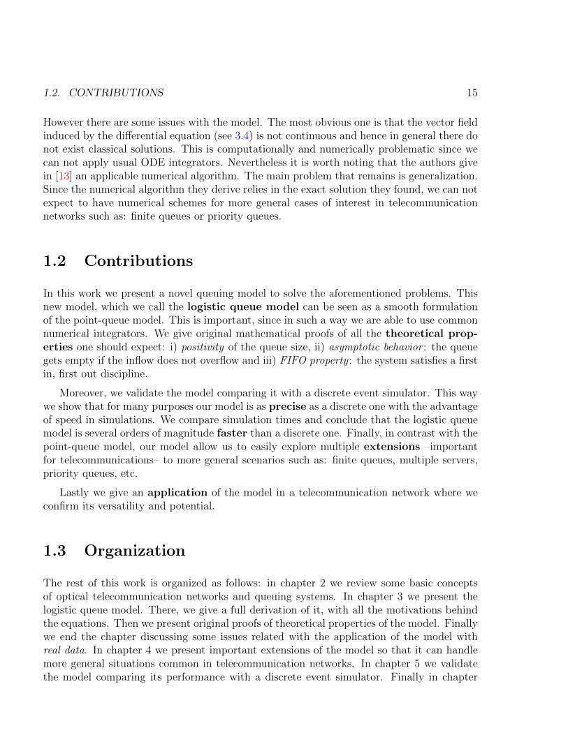
However there are some issues with the model. The most obvious one is that the vector fieldinduced by the differential equation (see 3.4) is not continuous and hence in general there donot exist classical solutions. This is computationally and numerically problematic since wecan not apply usual ODE integrators. Nevertheless it is worth noting that the authors givein [13] an applicable numerical algorithm. The main problem that remains is generalization.Since the numerical algorithm they derive relies in the exact solution they found, we can notexpect to have numerical schemes for more general cases of interest in telecommunicationnetworks such as: finite queues or priority queues.
1.2 Contributions
In this work we present a novel queuing model to solve the aforementioned problems. Thisnew model, which we call the logistic queue model can be seen as a smooth formulationof the point-queue model. This is important, since in such a way we are able to use commonnumerical integrators. We give original mathematical proofs of all the theoretical prop-erties one should expect: i) positivity of the queue size, ii) asymptotic behavior : the queuegets empty if the inflow does not overflow and iii) FIFO property : the system satisfies a firstin, first out discipline.
Moreover, we validate the model comparing it with a discrete event simulator. This waywe show that for many purposes our model is as precise as a discrete one with the advantageof speed in simulations. We compare simulation times and conclude that the logistic queuemodel is several orders of magnitude faster than a discrete one. Finally, in contrast with thepoint-queue model, our model allow us to easily explore multiple extensions –importantfor telecommunications– to more general scenarios such as: finite queues, multiple servers,priority queues, etc.
Lastly we give an application of the model in a telecommunication network where weconfirm its versatility and potential.
1.3 Organization
The rest of this work is organized as follows: in chapter 2 we review some basic conceptsof optical telecommunication networks and queuing systems. In chapter 3 we present thelogistic queue model. There, we give a full derivation of it, with all the motivations behindthe equations. Then we present original proofs of theoretical properties of the model. Finallywe end the chapter discussing some issues related with the application of the model withreal data. In chapter 4 we present important extensions of the model so that it can handlemore general situations common in telecommunication networks. In chapter 5 we validatethe model comparing its performance with a discrete event simulator. Finally in chapter

16 CHAPTER 1. INTRODUCTION
6 we give an application of the model to show its potential. The report ends with someconcluding remarks.

Chapter 2
Background
In this chapter we review some basic concepts of optical networks and queuing systems.
2.1 Introduction to dynamic optical networks
An optical network can be defined as a graph with its representative equipment based ona certain optical technology. In general, it is represented by an undirected graph wherethe edges are fiber optic links and the vertices are optical nodes capable of establishing anddeleting optical connections. The optical technology uses a range of frequencies of the totalOptical Spectrum (OS), and it is measured in Gigahertz (GHz). The capacity of an opticallink depends on the OS width and other factors like the spectral efficiency of establishedconnections. This part of the network is called the optical layer.
On top of the above described optical layer, large packet nodes (e.g. IP routers orEthernet switches) are collocated, they serve as end points of network traffic, as well assupport intermediate transit operation. Thus, a traffic flow is a request of bitrate to betransported between a source packet node and a termination packet node usually expressedin Megabits per second (Mb/s) or Gigabits per second (Gb/s). When a demand is accepted,an optical connection in the network is established between source and termination nodes;these optical connections are called lightpaths since they allow the data transmission as alight wave.
From the abstracted view of the packet layer, a lightpath is considered as a virtual linkdirectly connecting two packet nodes. In this layer, data is transmitted discretely in the formof packets. Packet sizes are usually measured in bytes (1 byte is equal to 8 bits). Thus,a virtual topology is used to route and serve traffic between source and destination nodes.Hence we have two layers in the network: the physical layer –the optical layer– where data istransmitted as a light wave and a virtual layer –the packet layer– where data is transmittedin the forms of packets.
17

18 CHAPTER 2. BACKGROUND
In the packet layer is where we have queues and servers. There is where our main focuswill be for the rest of this report. Packets are sent from a source packet node to a terminationpacket node using servers of given velocities (usually in Gb/s). When a packet finds a serveroccupied it enters into the waiting line, i.e. a queue, until the server becomes free and itcan be used.
Two different approaches can be considered for planning and operating communicationsnetworks: static and dynamic traffic scenarios. In static traffic scenarios, no changes areconsidered in the connections established during the working period of the network. Thus,the information about client demands to be served, i.e. the source and destination nodesand the required bandwidth, is known in advance. Since the routing of those demands canbe computed before the network begins to operate and no changes are allowed during theworking time, the optimality of the network planning is always kept.
On the contrary, in dynamic traffic scenarios demands are not known in advance andconnections are continuously set up and torn down. We assume that client requests arriveto the network following a certain probability distribution function. Moreover, connectionsremain active during a certain period of time, i.e. the service time, which can be also modeledby another probability function. In this scenario is where simulation and modeling comeinto play. Given a particular situation where we model client requests, network capacities(queues lengths, server speeds) network topology, etc; we can simulate the network andevaluate its performance.
Figure 2.1: Simplified network architecture example.
A simplified network architecture is presented in Figure 2.1, where an optical transportnetwork containing a set of packet nodes is interconnected by means of virtual links in thepacket layer. Each virtual link is supported by one or more optical connections in the opticallayer. Thus, traffic is served through such capacity.
The network in the example interconnects different access and metropolitan areas where

2.2. QUEUING MODELS 19
service end users are. All traffic generated in one area targeting other area in the operatordomain or another network (e.g. Internet) is aggregated in the source packet node and senttowards the destination node, thus becoming a traffic flow. For instance, in the exampleabove, the depicted OD flow can include at the same time: i) traffic between end users ofboth areas, ii) traffic between the source area and a large Data Center (DC), and iii) trafficfrom the small to the large DC.
2.2 Queuing models
Queueing theory is the study of waiting lines. Using mathematical and computational toolsa model is constructed so that queue lengths and waiting times can be predicted. In generalthere exist many types of queueing models, being the the probabilistic [14] the most com-mon ones. They are very important conceptually and theoretically, nevertheless we will notmake use of them explicitly.
The second most usual models are discrete event simulation systems. Before describ-ing in some detail how we can model a queue and a server using a discrete event simulatorwe will describe the functioning of our system in more intuitive terms.
Figure 2.2: Schematic picture of a system consisting of a server with a queue.
In Figure 2.2 we show a schematic picture that models a server with a queue. Entities (e.g.customers, packets) are generated from Generator following some probability distribution(e.g. exponential). Each entity is created at a specific instant of time. Then it has to beserved, if the Server is free when it was created, it is processed, else it joins the Queue. Weassume that the server has an associated speed µ, this means that our system is capable ofprocessing µ entities per unit of time. When the server gets free, the first entity in queuegoes to the server and abandons the waiting line. This type of queues are called first in, firstout (FIFO). Finally all entities end in a Sink where they are terminated.
Now we can describe the flow-chart associated to a discrete event simulator in moreprecise terms. A discrete event simulator consists of an ordered list of future events to be
20 CHAPTER 2. BACKGROUND
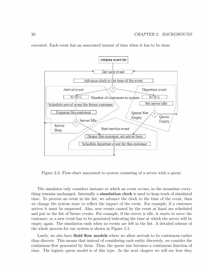
executed. Each event has an associated instant of time when it has to be done.
Figure 2.3: Flow-chart associated to system consisting of a server with a queue.
The simulator only considers instants at which an event occurs, in the meantime every-thing remains unchanged. Internally a simulation clock is used to keep track of simulatedtime. To process an event in the list, we advance the clock to the time of the event, thenwe change the system state to reflect the impact of the event. For example, if a customerarrives it must be enqueued. Also, new events caused by the event at hand are scheduledand put in the list of future events. For example, if the server is idle, it starts to serve thecustomer, so a new event has to be generated indicating the time at which the server will beempty again. The simulation ends when no events are left in the list. A detailed scheme ofthe whole process for our system is shown in Figure 2.3.
Lastly, we also have fluid flow models where we allow arrivals to be continuous ratherthan discrete. This means that instead of considering each entity discretely, we consider thecontinuous flow generated by them. Thus, the queue size becomes a continuous function oftime. The logistic queue model is of this type. In the next chapter we will see how they

2.3. SUMMARY 21
come up naturally as a consequence of a conservation law.
2.3 Summary
In this chapter we have given the basic concepts of optical dynamical networks relevant forthe rest of the report. The main idea is that data is transmitted discretely in the form ofpackets using servers from a source node to a destination node in the network. Moreoverwe have explained in some detail how we can use a discrete event simulator to model aserver with a queue. This is an important model because we will compare the performanceof the logistic queue model with it. It is important to stress that in contrast to a discreteevent simulator, the logistic queue model is a fluid flow model, which means that it does notconsider each packet independently but the flow generated by them. This will be the topicof next chapter.

22 CHAPTER 2. BACKGROUND

Chapter 3
The logistic queue model
In this chapter we present the logistic queue model. We give a full derivation of it, with allthe motivations behind the equations. Then we give original proofs of theoretical propertiesof the model. Finally we end the chapter discussing some issues related with the applicationof the model in a realistic data scenario.
3.1 Derivation
Assume we have a system with an inflow of entities arriving to a server of constant speedµ with an infinitely long queue as the one of Figure 3.1. In probabilistic terminology thesystem is denoted as G/D/1 [14]. We will derive an equation that relates the number ofentities in queue C with the inflow to the system f and the outflow g.
Figure 3.1: Example of a system with a queue and a server of speed µ.
Note that each quantity has the following units:
• [µ] = entities/time.
• [C] = entities.
• [f ] = [g] = entities/time.
23

24 CHAPTER 3. THE LOGISTIC QUEUE MODEL
We will assume that the amount of entities in queue C(t) in the instant t is a real number.This will be a reasonable approximation if the inflow is large enough: f � 1, physicallythis means that many entities arrive to the system (which is the case in telecommunicationnetworks). Also, this will make us not to distinguish between entities in queue and entitiesin the system. Therefore, for a short period of time dt the amount of entities that havearrived to the system is approximately f(t) · dt and likewise the number of them that haveabandoned it is g(t) · dt. This gives us the following conservation law:
C(t+ dt) = C(t) + f(t) · dt− g(t) · dt,
which in the limit when dt→ 0 reads:
C ′(t) = f(t)− g(t). (3.1)
We shall assume that there is a functional relationship between f, g and C, and expressthe outflow as a function of the inflow and the queue size:
g(t) = g(f, C) = µ+ e−αC(t) [min{µ, f(t)} − µ] . (3.2)
where:
1. µ > 0 is maximum outflow rate of the server.
2. α is a positive parameter taken to be ρµ, where ρ = λ
µis the average intensity, λ is the
mean of the inflow to the system:
λ = 1t1−t0
∫ t1
t0
f(t)dt
and [t0, t1] is the interval of definition of f .
The rationale behind this definition of α = ρµ
is the following: dividing by µ normalizesthe queue size, and weighting by ρ takes into account the intensity of the inflow. Note thatby construction we have:
1. If at t the queue is empty, i.e. C(t) = 0, then the outflow is just min{µ, f(t)}.
2. If the inflow is bigger than the maximum capacity, i.e. f(t) > µ, then the outflow isjust µ.
3. If C(t)→ +∞ then the outflow tends to µ.
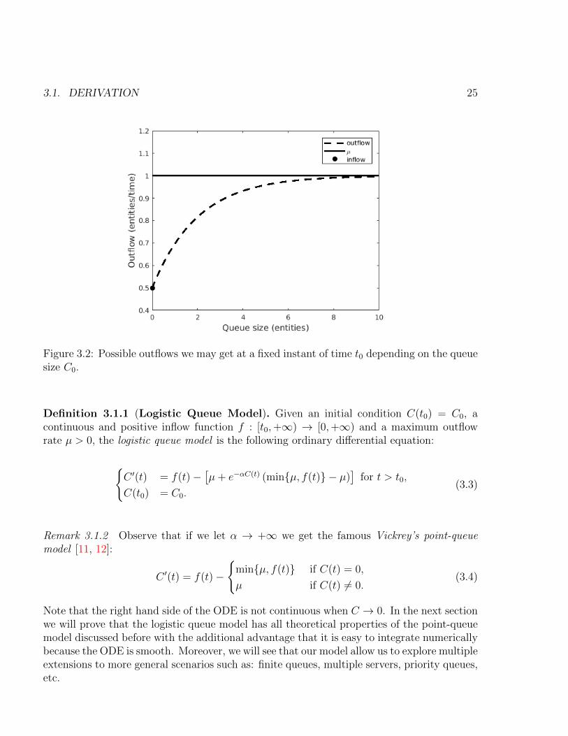
It is instructive to have a qualitative idea of how the outflow depends of the queue size. InFigure 3.2 we make a plot of g = g(f0, C0) for a fixed time t0 and varying C0 = C(t0).
In the picture we are assuming that f(t0) = 0.5. It is important to stress that this figurereflects all possible outflows we may get at a fixed instant of time t0 depending on the queuesize C0 we have. Finally we put together (3.1) and (3.2) in the following definition:
3.1. DERIVATION 25
Figure 3.2: Possible outflows we may get at a fixed instant of time t0 depending on the queuesize C0.
Definition 3.1.1 (Logistic Queue Model). Given an initial condition C(t0) = C0, acontinuous and positive inflow function f : [t0,+∞) → [0,+∞) and a maximum outflowrate µ > 0, the logistic queue model is the following ordinary differential equation:
{C ′(t) = f(t)−
[µ+ e−αC(t) (min{µ, f(t)} − µ)
]for t > t0,
C(t0) = C0.(3.3)
Remark 3.1.2 Observe that if we let α → +∞ we get the famous Vickrey’s point-queuemodel [11, 12]:
C ′(t) = f(t)−
{min{µ, f(t)} if C(t) = 0,
µ if C(t) 6= 0.(3.4)
Note that the right hand side of the ODE is not continuous when C → 0. In the next sectionwe will prove that the logistic queue model has all theoretical properties of the point-queuemodel discussed before with the additional advantage that it is easy to integrate numericallybecause the ODE is smooth. Moreover, we will see that our model allow us to explore multipleextensions to more general scenarios such as: finite queues, multiple servers, priority queues,etc.

26 CHAPTER 3. THE LOGISTIC QUEUE MODEL
3.2 Theoretical Properties
In this section we prove theoretical properties of the model. Let’s start with existence,uniqueness and positivity.
Proposition 3.2.1 (Existence, Uniqueness and Positivity). Given an initial conditionC(t0) = C0 ≥ 0, a continuous and positive inflow function f ≥ 0 and a maximum outflowrate µ > 0, we have that there exist a unique continuous differentiable solution C(t) to thesystem (3.3) defined in an interval [t0, Tmax) for Tmax ≤ +∞. Moreover such solution isalways greater or equal than zero.
Proof. Existence, uniqueness and differentiability of C(t) in an interval [t0, Tmax) for Tmax ≤+∞ is an easy consequence of the fact that the right hand side of (3.3) is a smooth functionof the variable C and it is continuous in t, hence we can apply Cauchy-Lipschitz theorem [15].Let us prove now positivity. Assume that for some time t− > t0 we have that C(t−) < 0.Then, since C(t) is continuous and C0 ≥ 0, there must be a t+ and a t∗ such that t+ < t∗ < t−where C(t+) ≥ 0 and C(t∗) = 0 (see Figure 3.3). Also, after reducing the interval I = [t+, t−]if necessary, we may assume that C(t) is strictly decreasing there. Therefore we have:
C ′(t) ≤ 0 in I = [t+, t−].
Figure 3.3: C is decreasing in [t+, t−].
Let’s see how this implies that f(t) ≤ µ in I. Indeed if f(t) > µ for some t ∈ I we wouldhave using (3.3) that C ′(t) = f(t)− µ > 0, which is a contradiction. Hence we deduce that
3.2. THEORETICAL PROPERTIES 27
C(t) ≡ 0 is a solution of{Q′(t) = f(t)−
[µ+ e−αQ(t) (min{µ, f(t)} − µ)
]for t ∈ I,
Q(t∗) = 0,(3.5)
which is impossible because we would have two different solutions C and C of (3.5) inI.
Remark 3.2.2 As a consequence of the previous proposition we deduce that if the queuestarts empty, i.e. C(t0) = 0, and the inflow is always smaller than the maximum outflowrate:
f(t) < µ for all t ≥ t0,
then the queue remains empty for all times and the outflow is equal to the inflow.
Now we are ready to prove some asymptotic properties of the queue:
Proposition 3.2.3 (Asymptotic behavior). Let C(t0) = C0 ≥ 0 be an initial condition,f ≥ 0 a continuous and positive inflow function and µ > 0 a maximum outflow rate. Thenthe solution of (3.3) is defined for all times, i.e. it is defined in the interval [t0,+∞).Moreover if the inflow satisfies:
f(t) ≤ f∞ < µ for all t ≥ tf (3.6)
for some time tf > t0 thenlimt→+∞
C(t) = 0.
Proof. Note that we can rewrite (3.3) as:
C ′(t) = f(t)− µ+ e−αC(t) (µ−min{µ, f(t)}) , (3.7)
but since C(t) ≥ 0 we have that e−αC(t) ≤ 1, and moreover µ−min{µ, f(t)} ≤ µ. Hence wededuce that:
C ′(t) ≤ f(t)− µ+ µ = f(t),
so finally we get that:
C(t) ≤ C0 +
∫ t
t0
f(s)ds.
Therefore C(t) is defined for all times since f is continuous and hence integrable. Assumenow that f satisfies (3.6). Then, using (3.7), we get:
C ′(t) = (1− e−αC(t)) · (f(t)− µ)
≤ (1− e−αC(t)) · (f∞ − µ), for all t ≥ tf .
28 CHAPTER 3. THE LOGISTIC QUEUE MODEL
Now, it is well known that the exponential satisfies:
eαC =∞∑n=0
(αC)n
n!≥ 1 + αC, for all C ≥ 0.
Hence,
e−αC ≤ 1
1 + αC⇔ 1− e−αC ≥ 1− 1
1 + αC=
αC
1 + αC.
Now, since (f∞ − µ) < 0 we get the following inequality:
C ′ ≤ αC · (f∞ − µ)
1 + αC.
Calling β = µ− f∞ > 0 and rearranging terms we obtain:
(1 +1
αC) · C ′ ≤ −β ⇔ d
dt
(C +
logC
α
)≤ d
dt(−βt) .
Therefore, integrating from tf to t,
C(t) +logC(t)
α≤ −βt+ k, for all t ≥ tf
where k = Cf +logCfα
+ βtf and Cf = C(tf ). Applying the exponential in both sides of theinequality one gets:
C1/α · eC ≤ e−βt+k. (3.8)
Finally, last equation implies that
C(t) ≤ eα(k−βt), for all t ≥ tf .
So the queue gets empty exponentially fast as stated.
Remark 3.2.4 Equation (3.8) gives us an estimate of how fast the queue goes to zero.Assuming (3.6) and given a fixed tolerance ε > 0, if we impose that:
C(t) ≤ eα(k−βt) · e−αC(t) ≤ ε,
then we find that the emptying time Tε(Cf ) ≥ tf needed to empty the queue within atolerance ε > 0 satisfies the following bound:
Tε(Cf ) ≤ tf +Cf − εµ− f∞
+1
α · (µ− f∞)· log
(Cfε
). (3.9)
Note that the previous equation has the following expected physical properties:

3.2. THEORETICAL PROPERTIES 29
1. The fastest way to empty the queue is by stopping the inflow, i.e. taking f∞ = 0. Onthe other hand, if f∞ → µ then the bound goes to infinity as expected.
2. If α→ +∞ then we get that the bound is equal to the emptying time of the point-queuemodel (3.4).
3. The bound is optimal because if we take ε = Cf then we deduce that Tε(Cf ) = tf .
�
Example 3.2.5 Constant inflow. Assume that the inflow to the system is constant, i.e.f(t) ≡ f∞ < µ. Fix also some C0 > 0 and t0 = 0. Then we have that (3.3) reduces to:{
C ′(t) = f∞ −[µ+ e−αC(t) (f∞ − µ)
]for t > 0,
C(0) = C0.(3.10)
This can be easily integrated, so we get the following explicit formula:
C(t) =1
αlog(1 + keγt
)(3.11)
where γ = α · (f∞ − µ) < 0 and k = eαC0 − 1 > 0. From the formula above is clear thatC(t) ≥ 0 and that limt→+∞C(t) = 0 as expected (see Figure 3.4).
Figure 3.4: Plot of queue size (3.11) for constant inflow f(t) ≡ 0.5 with µ = 1, α = 12
andC0 = 1.

30 CHAPTER 3. THE LOGISTIC QUEUE MODEL
Let’s now compare the bound we got in previous remark for the emptying time:
Tε(C0) =C0 − εµ− f∞
+1
α · (µ− f∞)· log
(C0
ε
), (3.12)
with the exact one we get with the analytical solution:
Tε(C0) =1
α · (µ− f∞)· log
(eαC0 − 1
eαε − 1
). (3.13)
Note that we have the following:
1. Tε(C0) ≤ Tε(C0) as we already know.
2. In the limit:
limα→+∞
Tε(C0) =C0 − εµ− f∞
.
So we recover the emptying time of the point-queue model.
3. When both C0 and ε are small, we have that eαC0−1eαε−1 ≈
C0
ε. Hence T and T only differ
by the linear term C0−εµ−f∞ .
To conclude this example in Figure 3.5 we make a plot of T and T with respect to C0 andfor µ = 1, f∞ = 0.5, α = 1
2and ε = 0.05.
Figure 3.5: Comparison of Tε and Tε for µ = 1, f∞ = 0.5, α = 12
and ε = 0.05.

3.2. THEORETICAL PROPERTIES 31
As already said, we can see in the plot that the bound is pretty accurate when C0 issmall, afterwards it deteriorates. �
To end this section we will show that our model satisfies the FIFO (first-in first-out)property, this is, that the entity that arrives first to the queue is also the one that gets outfirst. To accomplish this, we introduce the exit time of an entity that has arrived in theinstant t as:
Λ(t) = t+C(t)
µ. (3.14)
The rationale behind this definition is the following: C(t)/µ has units of time and itrepresents approximately the amount of time needed for emptying the queue if no moreentities arrived after t.
We have the following proposition:
Proposition 3.2.6 (FIFO property). Let C(t0) = C0 ≥ 0 be an initial condition, f ≥ 0a continuous and positive inflow function and µ > 0 a maximum outflow rate. Then
If t < s we have that Λ(t) < Λ(s).
In other words the exit time of an entity that has arrived in the instant t is smaller thanother that arrives at s > t.
Proof. We have that Λ(t) < Λ(s) is equivalent to:
C(s)− C(t)
s− t> −µ. (3.15)
Since C is differentiable, by the Mean-Value theorem [17] we know that there exists a ξ ∈ (t, s)such that
C ′(ξ) =C(s)− C(t)
s− t.
Now, we distinguish two cases:
1. f(ξ) < µ. There are two sub-possibilities:
• C(ξ) = 0. In this case C ′(ξ) = f(ξ)− f(ξ) = 0 > −µ, so (3.15) holds.
• C(ξ) > 0. In this case the outflow g satisfies 0 < g(ξ) < µ, hence
C ′(ξ) = f(ξ)− g(ξ) ≥ −g(ξ) > −µ.
2. f(ξ) ≥ µ. In this case C ′(ξ) = f(ξ)− µ > −µ, so (3.15) holds.

32 CHAPTER 3. THE LOGISTIC QUEUE MODEL
3.3 Applying the model
When we apply the logistic model with real data there are several considerations that mustbe taken into account. We discuss some of them in the following.
3.3.1 Discrete inflow
The inflow must be given to the logistic model in a continuous fashion. However in practicewe only see discrete entities arriving to the system. Hence we need to approximate our idealcontinuous inflow. In order to do this, we simply count how many entities have occurredeach dt seconds and then add them. In more mathematical terms, in a point of the formti+1 = (i+ 1) · dt we put
f(ti+1) ≈1
dt
∑(entities occurring in [i · dt, (i+ 1) · dt]) .
It may also be the case that we are already given the inflow at a discrete set of times, inthat case we do not need to deal with entities at all.
3.3.2 Integrating the ODE
Next we will need to solve the ODE (3.3). In order to do this we can use very standardmathematical algorithms for integrating differential equations. For example Runge-Kuttamethods [16]. The only caution one needs to take care of is the interpolation of the inflowbetween two successive points ti and ti+1. A linear interpolation usually suffices.
3.3.3 Queue error due to aggregation time
Approximating the inflow as discussed introduces an error in the model that we can notavoid but which we can estimate. Denote by Clog(t) the queue size given by the logisticqueue model, and by Cdisc(t) the real queue size. An entity that enters to the system att ∈ [i · dt, (i+ 1) · dt] will experience a delay of Cdisc(t)/µ seconds, nevertheless aggregatingeach dt seconds the model can not account the fact that the packet got in at t, hence:
|Cdisc(t)µ
− Clog(t)
µ| ≤ dt.
If the traffic is really intense, i.e. if ρ = λµ
is near one, the best we can expect for is:
|Cdisc(t)− Clog(t)| ∼ µ · (1− ρ) · dt. (3.16)
In chapter 5 we verify empirically previous equation.

3.4. SUMMARY 33
3.4 Summary
In this chapter we have presented the logistic queue model and its main theoretical properties.We have given original mathematical proofs of reasonable properties all queueing modelsought have: positivity of the queue, emptying of the queue and FIFO property. We haveseen how fluid flow models come up as a consequence of a conservation law. Then thelogistic queue model appears as a functional relationship of the queue size, the inflow andthe outflow. We have also discussed issues related to the application of the model with realdata. In the next chapter we will discuss extensions of the basic model which will turn outto be useful in the framework of telecommunication networks.

34 CHAPTER 3. THE LOGISTIC QUEUE MODEL

Chapter 4
Extensions for CommunicationNetworks
In this chapter we present variations of the model that allow us to address more generalscenarios present in telecommunication networks than the one assumed until now. Namely:
• If we have a probabilistic distribution on service times, i.e. a G/G/1 system.
• If we have a finite queue.
• If we have k servers, i.e. a G/D/k system.
• If two flows join in a server and then they separate following different paths.
• If we have priority queues.
Note that we may also have combinations of the previous cases.
4.1 Variable service times
Until this point we have assumed that µ is constant. Nevertheless it is very easy to see thatall results that we have proven are still valid even when µ = µ(t) depends on time as longas µ(t) ≥ 0 for all t.
4.2 Finite queue
Assume we are only able to store a finite number of entities Cmax > 0 in queue. We wouldlike to add this restriction to the model. The idea is to annihilate the inflow when the queue
35
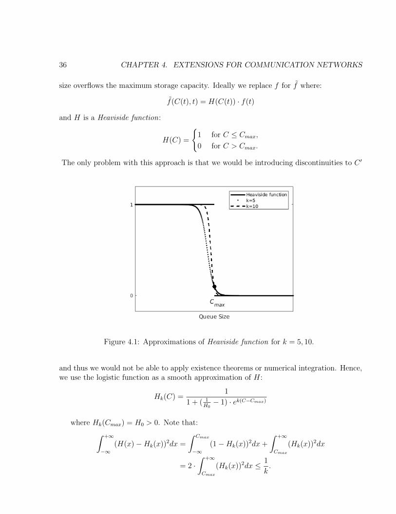
36 CHAPTER 4. EXTENSIONS FOR COMMUNICATION NETWORKS
size overflows the maximum storage capacity. Ideally we replace f for f where:
f(C(t), t) = H(C(t)) · f(t)
and H is a Heaviside function:
H(C) =
{1 for C ≤ Cmax,
0 for C > Cmax.
The only problem with this approach is that we would be introducing discontinuities to C ′
Figure 4.1: Approximations of Heaviside function for k = 5, 10.
and thus we would not be able to apply existence theorems or numerical integration. Hence,we use the logistic function as a smooth approximation of H:
Hk(C) =1
1 + ( 1H0− 1) · ek(C−Cmax)
where Hk(Cmax) = H0 > 0. Note that:∫ +∞
−∞(H(x)−Hk(x))2dx =
∫ Cmax
−∞(1−Hk(x))2dx+
∫ +∞
Cmax
(Hk(x))2dx
= 2 ·∫ +∞
Cmax
(Hk(x))2dx ≤ 1
k.
4.2. FINITE QUEUE 37
Hence Hk → H as k → +∞ in the L2 norm. This convergence is shown in Figure 4.1.
Therefore we obtain the following logistic finite-queue model:{C ′(t) = f(C(t), t)−
[µ+ e−αC(t)
(min{µ, f(C(t), t)} − µ
)]for t > t0,
C(t0) = C0.(4.1)
wheref(C(t), t) = Hk(C(t)) · f(t).
Theorem 4.2.1. Let C(t0) = C0 ≥ 0 be an initial condition, f ≥ 0 a continuous and positiveinflow function, µ > 0 a maximum outflow rate and Cmax > 0 a maximum queue capacity.Then we have that the system (4.1) satisfies the following properties:
1. There exists a unique an positive solution defined for all times.
2. If the inflow is strictly smaller than the maximum outflow rate then the queue getsempty exponentially fast.
3. FIFO: the exit time of an entity that has arrived in the instant t is smaller than otherthat arrives at s > t.
4. If C0 < Cmax and the inflow satisfies that
f(t) ≤Mf for all t ≥ t0 for some Mf > 0, (4.2)
then there exists a H0 > 0 and a k > 0 such that Hk approximates H as precisely asdesired (in the L2 sense) and moreover
C(t) ≤ Cmax for all t ≥ t0.
Proof. Properties 1,2 and 3 follow because the right hand side of (4.1) is locally Lipschitzcontinuous [15] so we can apply again existence and uniqueness, and afterwards repeatanalogous arguments like the ones given in the previous chapter. Let’s prove propertynumber 4. Assume there is a t′ > t0 such that C(t′) > Cmax. Since C(t0) < Cmax, theremust exist a t∗ such that C(t∗) = Cmax. We shall assume that in a sufficiently small intervalI around t∗ the function C(t) is strictly increasing, so that C ′(t) > 0 for t ∈ I. Analogouslyas in the proof of Proposition 3.2.1 we must have that f > µ in I. Hence
C ′(t∗) = f(C(t∗), t∗)− µ = H0 · f(t∗)− µ≤ H0 ·Mf − µ = 0
where we have taken H0 = µMf
. Whence we get a contradiction, so the queue remains
bounded by Cmax for all times.

38 CHAPTER 4. EXTENSIONS FOR COMMUNICATION NETWORKS
4.3 Multiple servers
Assume we have k servers of speed µ0. When an entity arrives to the system it goes to thefirst server that finds empty and else goes to the queue. The key modification of (3.3) now,is to make µ = µ(C(t)) dependent of the queue size. We take:
µ(C(t)) =
{µ0k if C(t) ≥ k − 1,
µ0 (1 + C(t)) if C(t) ≤ k − 1.(4.3)
The idea behind this equation is the following: if there are no entities in queue and onearrives it gets served at speed µ0 as usual. On the other hand, if there are, say, 5 entitiesin queue and 1 more arrives, we should have 5+1 servers functioning in order to serve all 6entities. Hence the total speed of the system would be 6µ0.
4.4 Separation of flows
Assume f1 and f2 are two inflows that join in a system with a server and a queue as inFigure 4.2. They are processed in that system but afterwards they follow different paths.Denote by g1 and g2 the corresponding outflows.
Figure 4.2: Two flows join in a server with a queue and then each of them follow a differentpath.
We can obtain them with a very simple argument. If we denote by f = f1 + f2 andprocess this inflow, we get an aggregated outflow g. Then, for each t we should have that:
f1(t)
f(t)=g1(t)
g(t),
henceg1(t) = g(t)
f(t)· f1(t).
4.5. PRIORITY QUEUES 39
Likewise,g2(t) = g(t)
f(t)· f2(t).
Note that this way we have that g1(t) + g2(t) = g(t) as expected. A similar argument canbe given in the case we have more than two flows.
4.5 Priority queues
Assume again f1 and f2 are two inflows that join in a system with a server of fixed speed µ.The only difference is that this time we assume that the flow f1 has a priority over f2, i.e.entities coming from f1 will be served first than entities from f2. We will model separatelythe queues formed by each flow:{
C ′1(t) = f1(t)−[µ1 + e−α1C1(t) (min{µ1, f1(t)} − µ1)
],
C ′2(t) = f2(t)−[µ2 + e−α2C2(t) (min{µ2, f2(t)} − µ2)
],
(4.4)
where we impose that µ1 + µ2 = µ. The key idea now is to take:
µ2(C1(t)) =f2(t)
f(t)µe−βC1(t)
where f = f1 + f2. Also we take µ1(C1(t)) = µ− µ2(C1(t)). Observe that:
1. If C1 = 0 then µ1 = f1fµ and µ2 = f2
fµ so each speed is proportional to its inflow
weight.
2. If C1 → +∞ then µ1 → µ and µ2 → 0 so just the priority one entities are served andthe others are not.
4.6 Summary
In this chapter we have presented variations of the basic logistic queue model that allow usto address more general scenarios present in telecommunication networks. This is one of themain advantages of our model over others. We have shown how we can modify slightly themain equation to include important cases such as: finite queues and priority queues. Thiswill be useful in chapter 6 when we present an application of the model in a network.

40 CHAPTER 4. EXTENSIONS FOR COMMUNICATION NETWORKS

Chapter 5
Validation and Results
In this chapter we validate the logistic queue model comparing its performance with a discreteevent simulator.
5.1 Notations
In this section we recall all our notation and its meaning. They will be used throughly inthe following sections.
- Maximum outflow rate: µ. Its units are entities/time. It will be assumed to beconstant, for example, µ = 1 Gb/s. It is given, so it is an input.
- Queue size at t: C(t). Its units are entities. It varies over time. Our goal is to predictthis quantity.
- Inflow to the system at t: f(t). Its units are entities/time. It varies over time. It isgiven, so it is an input.
- Outflow of the system at t: g(t). Its units are entities/time. It varies over time. Ourgoal is to predict this quantity.
- Mean inflow : λ. Its units are entities/time. It is the mean of the inflow f .
- Mean intensity or occupancy : ρ. It has no units. It is defined as λµ. This quantity
gives us an idea of the average use of the server.
- Aggregation time: dt. Its units are time. When a flow is given in discrete form, we willassume it is given each dt seconds. Usually dt = 60.
- Logistic model parameter : α. It is defined as ρµ.
41

42 CHAPTER 5. VALIDATION AND RESULTS
5.2 Error measures
In the following sections we will compare the queue size given by the logistic queue model,which we denote Clog(t), with the queue size given by a discrete packet simulator, which wedenote Cdisc(t). In order to compare them we need some error measures. Most of the timethose quantities are given at discrete instants of time. So in the end we will only have twovectors Cdisc,Clog evaluated at a finite number of times n. Since the logistic model will notreact to small fluctuations in the queue, we will be mostly interested in checking if the modelcaptures big queues. These are the important ones because they affect the outflow the most.We define:
1 Error relative to the maximum:‖Cdisc −Clog‖‖1 ·max (Cdisc) ‖
where 1 is vector of ones of length n.
2 Maximum occupancy error :
|max (Cdisc)−max (Clog) ||max (Cdisc) |
.
Likewise, we will want to compare the outflow given by the logistic queue model, which wedenote glog(t), with the outflow given by the discrete Simulink simulator, which we denotegdisc(t). Again, in order to compare them we need some error measures. Most of the timethose quantities are given at discrete instants of time. So in the end we will only have twovectors gdisc = (g1
disc, . . . , gndisc) and glog = (g1
log , . . . , gnlog) evaluated at a finite number of
times n. We define:
3 Mean relative outflow error :1
n
n∑i=1
|gidisc − gilog||gidisc|
4 Global relative error :‖gdisc − glog‖‖gdisc‖
5.3 User service characterization
In order to test the logistic queue model, we will model and simulate realistic traffic flows.In the following we will focus in video flows due to the easiness of characterization, but theextension to other kind of services is straightforward. We will model the inflow created bya video user in a discrete way, i.e. packet by packet.

5.3. USER SERVICE CHARACTERIZATION 43
For characterizing video streaming, an on-demand video file was served from a set ofHTTP servers to a single end user based on the MPEG-DASH v1.4 standard. On the server-side, two virtual machines each running an Apache HTTP server instance were responsiblefor serving the audio and the video components, respectively. The video was served at HD720p and its duration was 10 minutes.
Now, we will make some statistical assumptions about the packets generated while usinga video service:
1. All packets are assumed to be of the same constant size.
2. Packets are assumed to come in bursts of variable size. We will assume that the sizeof each burst follows a Normal distribution.
3. Bursts are assumed to be separated by variable intervals of time. We will assumethat the size of an interval of time separating two bursts –Interburst time– follows anExponential distribution.
4. Finally, packets are assumed to be separated by variable intervals of time inside aburst. We will assume that the size of an interval of time separating two packets insidea burst –Interpacket time– also follows an Exponential distribution.
Once the real video flows were generated, the parameters of each distribution were estimatedusing standard statistical methods. We obtained the results of Table 5.1.
Table 5.1: Estimation of parameters for a video user.
Packet size (Bytes) 1464Burst size (mean) 1714Burst size (variance) 278Interburst time (seconds) 5.56Interpacket time (seconds) 0.00345
Next we want to model the use of video service. Since we are interested in simulatingmore than a few hours, we cannot assume that each video user is watching video continuouslywithout stopping.
Hence we assume that uses of the service are separated by an interval of time –Interusetime– following an Exponential distribution with mean 45 minutes. So in mean, a typicaluser watches some videos each forty five minutes. Finally, we know from experience that notall videos are of the same length, and even if they were, it is possible and usual to watchmore than one. Therefore we also assume a probability distribution on video consumptionslisted in Table 5.2.

44 CHAPTER 5. VALIDATION AND RESULTS
Table 5.2: Length of video consumptions and their probabilities.
Video use (minutes) Probability5 0.4
15 0.330 0.25120 0.05
Using all previous assumption we can simulate all packets generated by a video user. Itseasier to picture all the previous concepts with a figure. In Figure 5.1 we show a simulatedpacket flow using the previously estimated parameters.
Figure 5.1: Simulation of packets generated by a video user during two hours. Each blueline represents a packet.
Now we want to compute the flow fv it generates. In order to do this, we simply count howmany packets have occurred each dt = 60 seconds and then add them. In more mathematicalterms, in a point of the form ti+1 = (i+ 1) · dt we put
fv(ti+1) ≈1
dt
∑(packets occurring in [i · dt, (i+ 1) · dt]) .
In Figure 5.2 we plot the flow generated by a typical video user. As it is expected, theservice is not being used constantly, but rather sparely as wanted.

5.4. IMPLEMENTATION 45
Figure 5.2: Flow fv generated by one video user during two hours.
5.4 Implementation
As already said, in the following we will compare the queue size given by the logistic queuemodel with the queue size given by a discrete packet simulator. We implemented bothmodels using standard software:
1. The logistic queue model was implemented in MATLAB. The only thing that has to bedone is to solve the ordinary differential equation (3.3). In Matlab there are severallibraries for solving differential equations, being the most usual ones ode45 and ode113.Both functions give indistinguishable results.
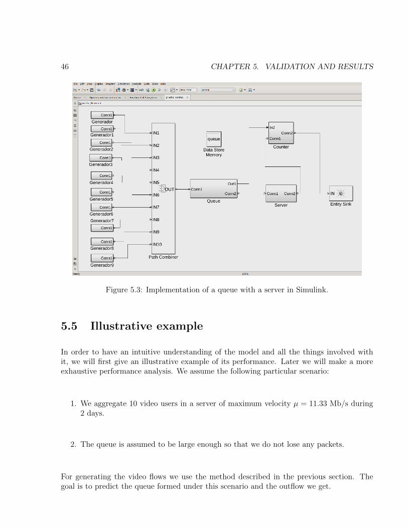
2. The discrete packets simulator was implemented in SIMULINK. Simulink is a block dia-gram environment for multidomain simulation and Model-Based Design. It supportssimulation, automatic code generation, and continuous test and verification of embed-ded systems. We can see a screenshot of part of the implemented system in Figure5.3.
46 CHAPTER 5. VALIDATION AND RESULTS
Figure 5.3: Implementation of a queue with a server in Simulink.
5.5 Illustrative example
In order to have an intuitive understanding of the model and all the things involved withit, we will first give an illustrative example of its performance. Later we will make a moreexhaustive performance analysis. We assume the following particular scenario:
1. We aggregate 10 video users in a server of maximum velocity µ = 11.33 Mb/s during2 days.
2. The queue is assumed to be large enough so that we do not lose any packets.
For generating the video flows we use the method described in the previous section. Thegoal is to predict the queue formed under this scenario and the outflow we get.

5.5. ILLUSTRATIVE EXAMPLE 47
Inflow
Adding the 10 video flows we get the inflow of Figure 5.4. In other words we put
f(t) =10∑v=1
fv(t).
Figure 5.4: Inflow to the system. Its standard deviation is 2.53 Mb/s.
The mean of the inflow is λ = 6 Mb/s, hence the average intensity is ρ = 53%. Thereforewe take α = ρ
µ= 0.05. As we see in the picture, during some periods of time, the inflow is
bigger than the maximum outflow µ, therefore in those moments we expect the queue sizeto increase.
Comparison of queues
We feed the inflow f to both the Simulink discrete model and to the logistic queue modeland compare the queue results we get in both cases. Note that f is given to the discretesimulator in discrete form, i.e. packet by packet as it was generated, whereas to the logisticmodel the inflow is given in a continuous fashion, i.e. aggregated each 60 seconds and thenlinearly interpolated when needed. Just looking at Figures 5.5 and 5.6 of the queues formedis impossible to tell the difference, hence we need some metrics to compare them. We willuse the two measures introduced before:
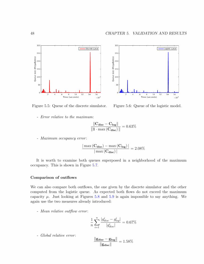
48 CHAPTER 5. VALIDATION AND RESULTS
Figure 5.5: Queue of the discrete simulator. Figure 5.6: Queue of the logistic model.
- Error relative to the maximum:
‖Cdisc −Clog‖‖1 ·max (Cdisc) ‖
= 0.63%
- Maximum occupancy error :
|max (Cdisc)−max (Clog) ||max (Cdisc) |
= 2.08%
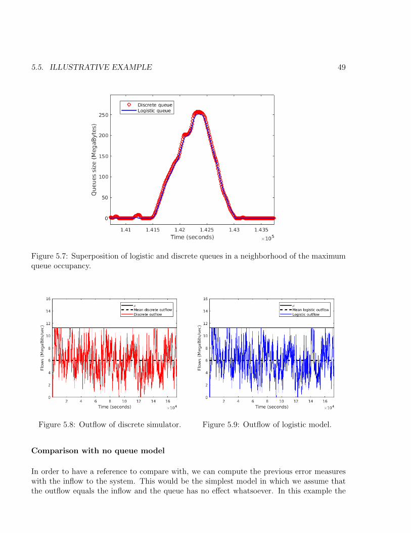
It is worth to examine both queues superposed in a neighborhood of the maximumoccupancy. This is shown in Figure 5.7.
Comparison of outflows
We can also compare both outflows, the one given by the discrete simulator and the othercomputed from the logistic queue. As expected both flows do not exceed the maximumcapacity µ. Just looking at Figures 5.8 and 5.9 is again impossible to say anything. Weagain use the two measures already introduced:
- Mean relative outflow error :
1
n
n∑i=1
|gidisc − gilog||gidisc|
= 0.67%
- Global relative error :‖gdisc − glog‖‖gdisc‖
= 1.58%
5.5. ILLUSTRATIVE EXAMPLE 49
Figure 5.7: Superposition of logistic and discrete queues in a neighborhood of the maximumqueue occupancy.
Figure 5.8: Outflow of discrete simulator. Figure 5.9: Outflow of logistic model.
Comparison with no queue model
In order to have a reference to compare with, we can compute the previous error measureswith the inflow to the system. This would be the simplest model in which we assume thatthe outflow equals the inflow and the queue has no effect whatsoever. In this example the

50 CHAPTER 5. VALIDATION AND RESULTS
mean relative error is:1
n
n∑i=1
|gidisc − f i||gidisc|
= 0.75%,
while the global relative error is:
‖gdisc − f‖‖gdisc‖
= 5.27%.
As expected mean-wise the relative errors are very similar. This is due to the fact that mostof the time the inflow is smaller than µ and hence the outflow g is equal to f . On the otherhand the global relative error is sensibly bigger for the no queue model since this measurepenalizes more point-wise errors.
Discussion of example
As already stated the goal of this example was to introduce in an intuitive fashion all conceptsinvolved with the model in a practical setting. The results are very promising in the sensethat our model captures very well the queue generated and hence also the outflow. At theend of the day, one may wonder why it is worth introducing a continuous model (the logisticqueue model) if we already can make discrete simulations and get quite accurate results.The key is of course scalability. In this illustrative example the simulation time of thediscrete simulator was around 60021 seconds, which is about 16 hours. On the other handto the logistic queue model the whole process only took about 29 seconds. So the continuousmodel is around 2000 times faster! This is expectable since the discrete simulator had toprocess around 2.45 · 107 entities. In the next section we will make a more comprehensiveanalysis of the performance of the model.
5.6 Performance Analysis
In this subsection we analyze how the error measures introduced in the previous examplesevolve as the intensity of the inflow is varied. Again we assume the same scenario as in theexample where we aggregate 10 video users in a server of maximum velocity µ = 11.33 Mb/sduring 2 days each 60 seconds.
We vary inflow intensities ρ from approximately 45% to 85%. In order to do so we simplyreduce the Interuse time introduced before when modeling a video user. Recall that thisparameter represented the amount of time between two uses of video service. Hence reducingit, we only make our 10 users watch videos more often. In total 21 simulations were launchedboth in the discrete event simulator implemented in Simulink and using the logistic queuemodel implemented in Matlab. Of the 21 simulations 3 of them had not finished after morethan a month in the discrete simulator, and therefore they were discarded. Note that in
5.6. PERFORMANCE ANALYSIS 51
each simulation we are generating around 25 million packets, so in total in 21 simulationswe generated about 500 million packets, which is roughly about 6000 GigaBytes of data.
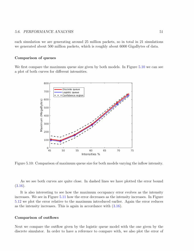
Comparison of queues
We first compare the maximum queue size given by both models. In Figure 5.10 we can seea plot of both curves for different intensities.
Figure 5.10: Comparison of maximum queue size for both models varying the inflow intensity.
As we see both curves are quite close. In dashed lines we have plotted the error bound(3.16).
It is also interesting to see how the maximum occupancy error evolves as the intensityincreases. We see in Figure 5.11 how the error decreases as the intensity increases. In Figure5.12 we plot the error relative to the maximum introduced earlier. Again the error reducesas the intensity increases. This is again in accordance with (3.16).
Comparison of outflows
Next we compare the outflow given by the logistic queue model with the one given by thediscrete simulator. In order to have a reference to compare with, we also plot the error of

52 CHAPTER 5. VALIDATION AND RESULTS
Figure 5.11: Maximum occupancy error of the logistic model varying the inflow intensity.
Figure 5.12: Error relative to the maximum of the logistic model varying the inflow intensity.

5.6. PERFORMANCE ANALYSIS 53
Figure 5.13: Global relative error of the outflows given by logistic model and the no-queuemodel varying the inflow intensity.
the no-queue model as discussed before. Recall that this just assumes that the queue hasno effect whatsoever so the outflows just equals the inflow. We begin by plotting the globalrelative error in Figure 5.13.
Note how the error of the no-queue model increases as the intensity increases. This is tobe expected because increasing the intensity increases the queue size and therefore makesthe outflow differ more from the inflow. On the other hand the error of the logistic queuemodel seems quite stable, its mean is around 2%.
Finally we compute the mean relative error. In Figure 5.14 we observe that until ρ = 55%there is no big difference between both models, both errors are quite low. This is again logicalsince we know that the outflow of the system is almost identical to the inflow when thereare not a big queues.
Scalability: simulation times
Now we want to compare the simulation time of both models. Since the mean simulationtime of the logistic model is 26.3 seconds but the mean of the discrete simulator is 7.6 dayswe apply the function log10.
As we see in Figure 5.15, the logistic queue model is about 5 orders of magnitude fasterthan the discrete simulator when the intensity of the inflow is about 60%. This is a hugedifference, the continuous model is 100, 000 times faster than the discrete one.

54 CHAPTER 5. VALIDATION AND RESULTS
Figure 5.14: Mean relative error of the outflows given by logistic model and the no-queuemodel varying the inflow intensity.
Figure 5.15: Simulation times of logistic and discrete queue model varying the inflow inten-sity.
5.7. SUMMARY 55
5.7 Summary
In this chapter we have validated the logistic queue model comparing its performance witha discrete event simulator. We have shown that:
• Our model is as precise as the discrete one. We compared queue sizes and outflow pre-dictions and the results show that differences are minimal. For example, the globalrelative error of the outflow given by the logistic model is only about 2%.
• Our model is several orders of magnitude faster than the discrete one. For example, whenthe mean intensity of the inflow is 60% the logistic model is about 100,000 times fasterthan the discrete one.
In the next chapter we will give an application of the logistic queue model in a scenariowhere a discrete simulation would be unfeasible. We will be dealing with flows of the orderof Gb/s.

56 CHAPTER 5. VALIDATION AND RESULTS
Chapter 6
Case study example
In this chapter we present a case study using the logistic queue model in a telecommunicationnetwork. Basically we study how the latency of the network is affected when we introducean external priority flow into play. We will be dealing with flows of the order of Gb/s, thisis where our model becomes useful, since running a discrete simulation for these orders ofmagnitude would be impossible.
6.1 Scenario
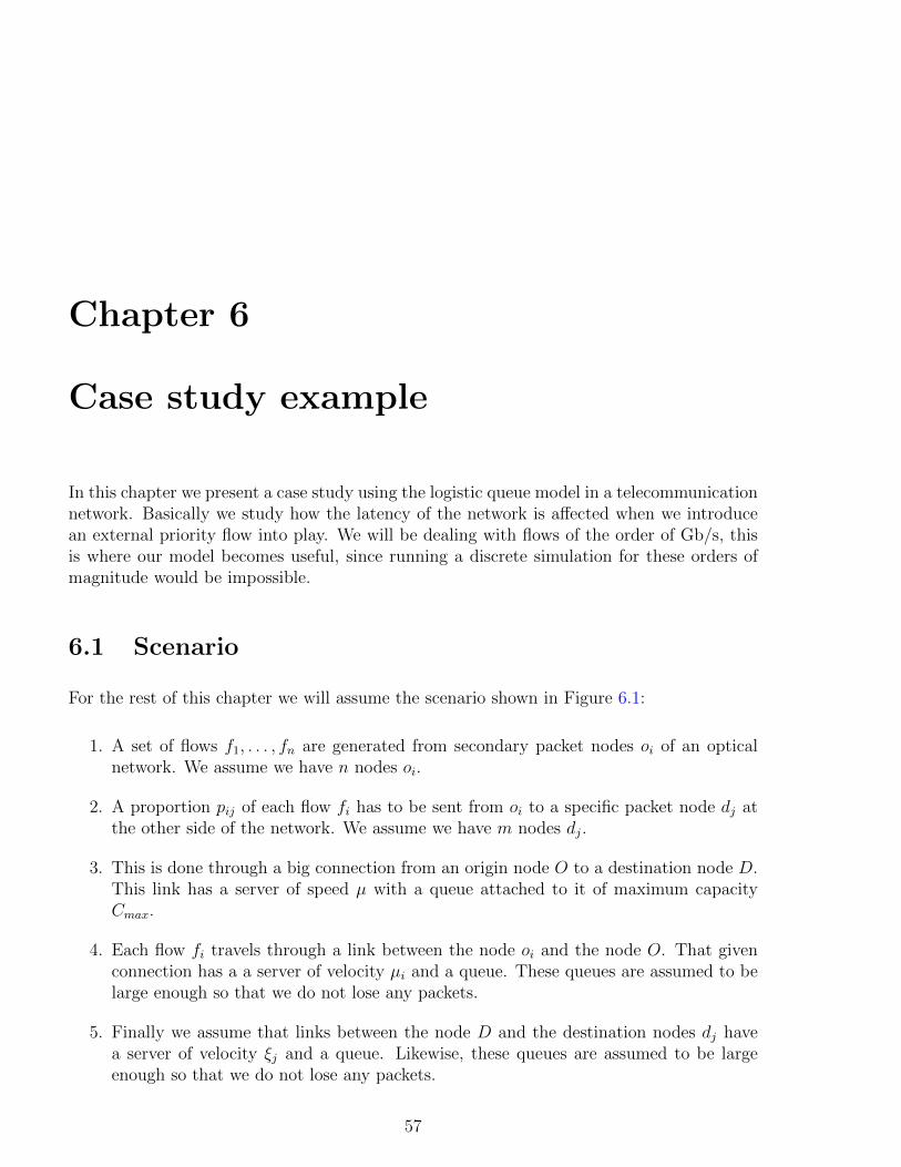
For the rest of this chapter we will assume the scenario shown in Figure 6.1:
1. A set of flows f1, . . . , fn are generated from secondary packet nodes oi of an opticalnetwork. We assume we have n nodes oi.
2. A proportion pij of each flow fi has to be sent from oi to a specific packet node dj atthe other side of the network. We assume we have m nodes dj.
3. This is done through a big connection from an origin node O to a destination node D.This link has a server of speed µ with a queue attached to it of maximum capacityCmax.
4. Each flow fi travels through a link between the node oi and the node O. That givenconnection has a a server of velocity µi and a queue. These queues are assumed to belarge enough so that we do not lose any packets.
5. Finally we assume that links between the node D and the destination nodes dj havea server of velocity ξj and a queue. Likewise, these queues are assumed to be largeenough so that we do not lose any packets.
57

58 CHAPTER 6. CASE STUDY EXAMPLE
In terms of entities (or packets) our network is equivalent to the one depicted in Figure6.2.
Figure 6.1: Network for the scenario in flow form. The goal is to send packets from regiono to region d of the network. In the picture n = 2 and m = 3.
Figure 6.2: Network for the scenario in packet form. The goal is to send packets from regiono to region d of the network. In the picture n = 2 and m = 3.
We will be mainly interested in computing the latency Lij(t) between node oi and nodedj at instant t. Physically this represent the amount of time it takes to a packet to travel

6.2. APPLYING THE LOGISTIC QUEUE MODEL 59
from oi to dj if it departures at t. In our system we have that:
Lij(t) =Coi (t) + s
µi+C(to) + s
µ+Cdj (td) + s
ξj,
where
- s is the size of each packet.
- Coi (t) is the queue formed between node oi and O at t.
- C(to) is the queue formed between node O and D at to.
- to is the instant at which the packet arrives to O: to = t+Coi (t)+s
µi.
- Cdj (td) is the queue formed between node D and dj at td.
- td is the instant at which the packet arrives to D: td = to + C(to)+sµi
.
It is easy to see that the previous formula can be generalized for more general networks.Moreover we define the expected latency of going from region o of the network to regiond as:
Lod(t) =1
n ·m∑i,j
Lij(t).
Finally we define the maximum expected latency as
Lmax = maxtLod(t).
We will be interested in studying how this quantity changes when we modify the scenariojust described above.
6.2 Applying the logistic queue model
Applying the model in the scenario just described is quite straightforward. First we processeach flow fi using the logistic queue model (3.3) to obtain flows gi. These are the outflowsof each oi and the inflows to O. Doing this we obtain the functions Co
i (t). Then we putg :=
∑ni=1 gi and process this flow using the logistic finite queue mode (4.1) to obtain a new
flow h. This is the outflow of O and the inflow to D. Doing this we obtain the function C(t).

60 CHAPTER 6. CASE STUDY EXAMPLE
Now, we must take into account the origin oi of each flow and its destination dj, hence by(4.4):
hj(t) =n∑i=1
pij ·(gi(t)
g(t)· h(t)
).
This is the outflow of D and the inflow to dj. Finally we process each hj using again thethe logistic queue model (3.3). Doing this we obtain the functions Cd
j (t).
6.3 Empirical results
- For generating the flows fi we use the method described in section 5.3 when we modeleda video user. In total n = 4 flows were generated during 1 day.
- Each flow fi consists of 10,000 video users, the mean inflow rate of each flow is about 12.5Gb/s. We take all µi = 25 Gb/s.
- For the big link OD we take µ = 100 Gb/s and Cmax = 25 GigaBytes.
- Since the mean of each flow fi is about 12.5 Gb/s and n = 4, we expect the use of the ODlink to be around 50%.
- We take m = 5 nodes dj. Each link has a speed of ξj = 20 Gb/s.
- Finally, the matrix pij is chosen to be:
p =
0.1293 0.3124 0.0548 0.2534 0.25010.1600 0.1681 0.0497 0.2203 0.40190.3029 0.0009 0.1687 0.2224 0.30510.0042 0.3710 0.2344 0.0250 0.3655
,so, for instance, 12.93% of the packets generated from node o1 go to node d1.
Then, in this setting we get the expected latency of Figure 6.3. We see that for a packetthat departs from region o of the network we expect that it takes at most 0.2 seconds toget to its destination in region d. The whole simulation took only about 2 minutes to becompleted.
6.4. SUMMARY 61
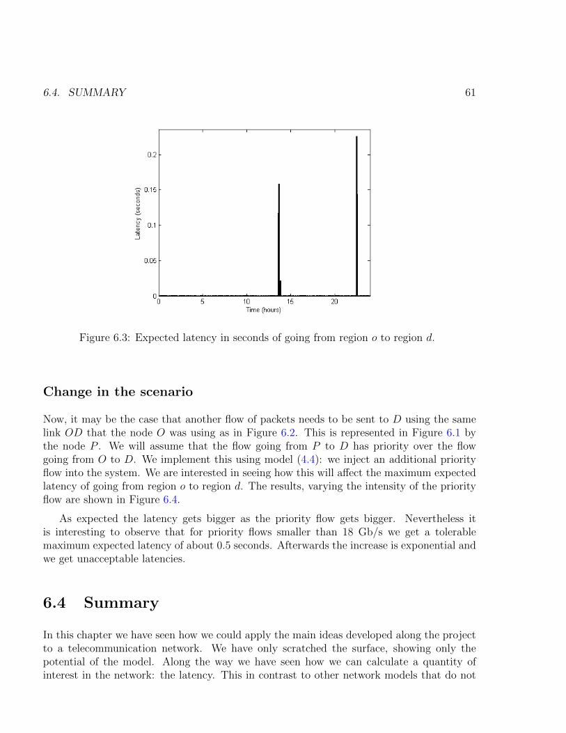
Figure 6.3: Expected latency in seconds of going from region o to region d.
Change in the scenario
Now, it may be the case that another flow of packets needs to be sent to D using the samelink OD that the node O was using as in Figure 6.2. This is represented in Figure 6.1 bythe node P . We will assume that the flow going from P to D has priority over the flowgoing from O to D. We implement this using model (4.4): we inject an additional priorityflow into the system. We are interested in seeing how this will affect the maximum expectedlatency of going from region o to region d. The results, varying the intensity of the priorityflow are shown in Figure 6.4.
As expected the latency gets bigger as the priority flow gets bigger. Nevertheless itis interesting to observe that for priority flows smaller than 18 Gb/s we get a tolerablemaximum expected latency of about 0.5 seconds. Afterwards the increase is exponential andwe get unacceptable latencies.
6.4 Summary
In this chapter we have seen how we could apply the main ideas developed along the projectto a telecommunication network. We have only scratched the surface, showing only thepotential of the model. Along the way we have seen how we can calculate a quantity ofinterest in the network: the latency. This in contrast to other network models that do not

62 CHAPTER 6. CASE STUDY EXAMPLE
Figure 6.4: Maximum expected latency in seconds of going from region o to region d varyingthe intensity of an extra priority flow in the simulation.
modelize queues of servers as stated in the introduction.

Chapter 7
Concluding Remarks
7.1 Contributions archieved
In this work we have presented a novel continuous queuing model called the logistic queuemodel. We have proven mathematically that our proposed model has many desirable the-oretical properties. Moreover, we validated the model comparing it with a discrete eventsimulator. We showed that in terms of queue size and outflow prediction our model is asprecise as a discrete one with the advantage of speed in simulations. We compared simula-tion times and concluded that the logistic queue model is several orders of magnitude fasterthan the discrete one. Finally in contrast with the point-queue model our model allow us toeasily explore multiple extensions to more general scenarios such as: finite queues, multipleservers, priority queues, etc. This in turn allowed us to show an application of all the toolsdeveloped.
7.2 Personal evaluation
Throughout this project I have applied many skills developed in the master program (MAMME).Specially useful have been the courses regarding modelling with differential equations andothers related to the numerical solution of them. Moreover, elective courses taken from thestatistics master (MESIO) have proven to be of conceptual help in the development of thethesis. Also, I have had to learn from scratch other important topics like discrete eventsimulators and the functioning of dynamic optical networks. This project enabled me toparticipate in the research Grup de Comunicacions Optiques (GCO) was conducting. I havehad the opportunity of learning how to read and compare research papers, how to studysome topics that I had not covered during my university courses, how to improve my pro-gramming skills (mostly in Simulink), how to modelize using mathematical tools, as well asthe capacity to solve relevant real world problems.
63

64 CHAPTER 7. CONCLUDING REMARKS
7.3 Future work
This work will be partially included as UPC contribution to the H2020 European METRO-HAUL project (G.A. no 761727). Specifically, a traffic generation tool will be defined andimplemented for creating realistic traffic traces exchanged in/between optical metro networks(metro flows). The tool (to be developed in Python) will basically consists in: i) a graphicaluser interface where different configuration parameters can be tuned, e.g. characteristicsand magnitude of individual user/service flows, periodic pattern, duration, etc; ii) a trafficgeneration engine that will receive input parameters to output metro flow traffic traces; andiii) a visualization module to easily check generated traffic flows, as well as different exportformats to facilitate the use of data for multiple use cases including network optimizationand analytics. The main contributions of this master thesis will be used to build a fast andaccurate traffic generation engine based on the logistic queue model.

Bibliography
[1] CISCO Global Cloud Index (GCI), 2015.
[2] CISCO Visual Networking Index (VNI), 2016.
[3] L. M. Contreras, V. Lopez, O. Gonzalez, A. Tovar, F. Munoz, A. Azanon,J.P. Fernandez-Palacios, and J. Folgueira: Towards cloud-ready transport net-works. IEEE Communications Magazine, vol. 50, pp. 48-55, 2012.
[4] D. King and A. Farrel: A PCE-based architecture for application-based networkoperations. CIETF RFC7491, 2015.
[5] V. Lopez and L. Velasco: Elastic Optical Networks: Architectures, Technologies,and Control. Ed. Springer, 2016.
[6] L. Velasco, A. Castro, M. Ruiz, and G. Junyent: Solving Routing and Spec-trum Allocation Related Optimization Problems: from Off-Line to In-Operation FlexgridNetwork Planning. IEEE/OSA Journal of Lightwave Technology (JLT), vol. 32, pp. 2780-2795, 2014.
[7] A.P. Vela, A. Vıa, F. Morales, M. Ruiz, and L. Velasco: Traffic generation fortelecom cloud-based simulation. IEEE International Conference on Transparent OpticalNetworks (ICTON), 2016.
[8] OMNeT++ Discrete Event Simulator: http://www.omnetpp.org/
[9] P. S. Barreto, T. F. Bento, Paulo H. P. de Carvalho: Multimedia NetworkSimulation with a Fluid Flow Model. IJCSNS International Journal of Computer Scienceand Network Security, VOL.10 No.6, June 2010.
[10] C. Kiddle, R. Simmonds, C. Williamson, and B. Unger: Hybrid Packet/FluidFlow Network Simulation. Proceedings of the Seventeenth Workshop on Parallel andDistributed Simulation (PADS?03) 1087-4097/03, IEEE 2003.
[11] Vickrey, W.S: Congestion theory and transport investment. The American EconomicReview 59 (2), 251261.
65

66 BIBLIOGRAPHY
[12] Ke Han, Terry L. Friesz, Tao Yao: A partial differential equation formulation ofVickrey’s bottleneck model, part I: Methodology and theoretical analysis. TransportationResearch Part B Methodological. March, 2013.
[13] Ke Han, Terry L. Friesz, Tao Yao: A partial differential equation formulation ofVickrey’s bottleneck model, part II: Numerical analysis and computation. TransportationResearch Part B Methodological. March, 2013.
[14] S.M. Ross: Introduction to Probability Models, Eleventh Edition. Academic Press.February, 2014.
[15] E. A. Coddington, N. Levinson: Theory of Ordinary Differential Equations. NewYork: McGraw-Hill.
[16] Arieh Iserles: A First Course in the Numerical Analysis of Differential EquationsCambridge Texts in Applied Mathematics, 2nd Edition.
[17] Michael Spivak: Calculus. Publish or Perish, 4th edition.