Technical Report No. 89/ Rapport technique no 89

Core Inflation

by Seamus Hogan, Marianne Johnson, and Thérèse Laflèche

Bank of Canada Banque du Canada

January 2001

Core Inflation

Seamus Hogan, Marianne Johnson, and Thérèse Laflèche

Research DepartmentBank of Canada

Ottawa, Ontario, Canada K1A 0G9mjohnson@bankofcanada.ca

The views expressed in this report are solely those of the authors. Noresponsibility for them should be attributed to the Bank of Canada.

Printed in Canada on recycled paper

ISSN 0713-7931

ISBN

ISSN 0713-7931

Printed in Canada on recycled paper

iii

v

vii

1

2

3

7

7

8

1

1

3

3

3

4

5

CONTENTS

Acknowledgments. . . . . . . . . . . . . . . . . . . . . . . . . . . . . . . . . . . . . . . . . . . . . . .

Abstract/Résumé. . . . . . . . . . . . . . . . . . . . . . . . . . . . . . . . . . . . . . . . . . . . . . .

1. Introduction. . . . . . . . . . . . . . . . . . . . . . . . . . . . . . . . . . . . . . . . . . . . . . . . .

2. Policy Purposes of a Measure of Core Inflation . . . . . . . . . . . . . . . . . . . . .

2.1 A good indicator of current and future trends in inflation . . . . . . . 2

2.2 A viable target for monetary policy . . . . . . . . . . . . . . . . . . . . . . . . 2

2.3 Which price index? . . . . . . . . . . . . . . . . . . . . . . . . . . . . . . . . . . . . .

3. A Model of Inflation Determination . . . . . . . . . . . . . . . . . . . . . . . . . . . . . . 4

4. Alternative Approaches to the Measurement of Core Inflation . . . . . . . . .

4.1 The modelling approach . . . . . . . . . . . . . . . . . . . . . . . . . . . . . . . . .

4.2 The statistical approach. . . . . . . . . . . . . . . . . . . . . . . . . . . . . . . . . .

4.2.1 Aggregate approach . . . . . . . . . . . . . . . . . . . . . . . . . . . . . . . . . 9

4.2.2 Disaggregated approach . . . . . . . . . . . . . . . . . . . . . . . . . . . .10

5. Practical Issues in the Measurement of Core Inflation . . . . . . . . . . . . . . . 1

5.1 Which approach to take?. . . . . . . . . . . . . . . . . . . . . . . . . . . . . . . . 1

5.2 What is the appropriate periodicity of the data for policy? . . . . . 12

5.3 Bias in price indexes . . . . . . . . . . . . . . . . . . . . . . . . . . . . . . . . . . . 1

6. Measures of Underlying Inflation at the Bank of Canada . . . . . . . . . . . . 1

6.1 CPIxFET as a measure of core inflation. . . . . . . . . . . . . . . . . . . . 1

6.2 Other measures of core inflation. . . . . . . . . . . . . . . . . . . . . . . . . . 1

7. An Evaluation of Various Measures of Underlying Inflation. . . . . . . . . . 18

7.1 As a good indicator of current and future trends in inflation . . . . 19

7.1.1 Does the core measure capture the persistent

movements or is it still volatile?. . . . . . . . . . . . . . . . . . . . . . . 19

7.1.2 Does the core measure help predict future trends

in inflation?. . . . . . . . . . . . . . . . . . . . . . . . . . . . . . . . . . . . . . . 20

7.1.3 Results of simple indicator models. . . . . . . . . . . . . . . . . . . . . 21

7.1.4 Properties of excluded components . . . . . . . . . . . . . . . . . . . . 21

7.1.5 Robustness. . . . . . . . . . . . . . . . . . . . . . . . . . . . . . . . . . . . . . . . 23

7.2 As a target for monetary policy . . . . . . . . . . . . . . . . . . . . . . . . . . 24

8. Conclusion . . . . . . . . . . . . . . . . . . . . . . . . . . . . . . . . . . . . . . . . . . . . . . . . 2

iv

27

0

5

4

0

References . . . . . . . . . . . . . . . . . . . . . . . . . . . . . . . . . . . . . . . . . . . . . . . . .

Figures . . . . . . . . . . . . . . . . . . . . . . . . . . . . . . . . . . . . . . . . . . . . . . . . .3

Tables . . . . . . . . . . . . . . . . . . . . . . . . . . . . . . . . . . . . . . . . . . . . . . . . .3

Appendix 1: Numerical Examples Demonstrating Core MeasureCalculations . . . . . . . . . . . . . . . . . . . . . . . . . . . . . . . . . . . . . . .40

Appendix 2: An Investigation of the Subcomponents of the CPI . . . . . . . . .4

Appendix 3: An Investigation of the Skewness and Kurtosis . . . . . . . . . . . .5

v

tina

nd

llent

nk for

anks

hted

ACKNOWLEDGMENTS

Thanks to Jean-Pierre Aubry, Allan Crawford, Chantal Dupasquier, Bet

Landau, Dave Longworth, and Tiff Macklem for their helpful discussions a

comments and to Frédéric Beauregard-Tellier and Richard Lacroix for exce

research assistance. The paper also benefited from discussions at the Ba

International Settlements 1999 Workshop of central bank model builders. Th

to Scott Roger for the methodology used to calculate measures of weig

skewness and weighted kurtosis.

vii

ofes intudyy bythatanddelrates

tentptualf core

thesed onwell

lapôtseursdanspour

rôledesLesit leaux

une desures de

ABSTRACT

The Bank of Canada usescoreCPI inflation, the year-over-year rate of changethe consumer price index excluding food, energy, and the effects of changindirect taxes, as the operational guide for monetary policy. In this report we sthe concept and measurement of core or underlying inflation more generallexamining several alternative measures of core inflation, from the viewpointcore inflation is a tool for policy purposes, either as an indicator of currentfuture trends in inflation, or as a viable target for monetary policy. A simple moof price determination is proposed that defines the core conceptually, and illustthe process by which aggregate inflation rates may differ from the core.

As a measure of inflation for policy purposes, core inflation is useful to the exthat it can be measured accurately. Therefore, following a discussion of conceissues, the report’s focus narrows and we introduce the various measures oinflation, concluding with a comparative evaluation of those measures. We findalternatives quite similar in many respects. However, a closer assessment batheir suitability to various policy purposes suggests that different measures doalong different dimensions.

JEL classification: E31Bank classification: Inflation and prices

RÉSUMÉ

La Banque du Canada a recours à l’inflationmesurée par l’indice de référence,c’est-à-dire le taux de variation sur douze mois de l’indice des prix àconsommation hors alimentation, énergie et effet des modifications des imindirects, pour la guider dans la conduite de la politique monétaire. Les autexaminent le concept et la mesure de l’inflation fondamentale ou sous-jacenteune perspective plus générale, en étudiant diverses méthodes possiblesmesurer l’inflation fondamentale. Ils partent du principe que celle-ci joue unutile dans la formulation de la politique monétaire, soit comme indicateurtendances actuelle ou future de l’inflation, soit comme cible à long terme.auteurs proposent un modèle simple de détermination des prix, qui définconcept de l’inflation fondamentale et illustre en quoi celle-ci peut différer du td’inflation global.

Aux fins de la conduite de la politique monétaire, l’inflation fondamentale estconcept utile pour autant qu’elle soit évaluée avec précision. Après une analysquestions d’ordre conceptuel, les auteurs se concentrent sur les diverses mes

viii

ve detrès

e laé.

l’inflation fondamentale et concluent leur exposé par une évaluation comparaticelles-ci. Les différentes mesures, constatent-ils, sont à maints égardssemblables. Toutefois, un examen attentif de leur utilité pour la conduite dpolitique monétaire indique que leurs mérites diffèrent selon le critère envisag

Classification JEL : E31Classification de la Banque : Inflation et prix

1

epinges bytaryakingotallyures,omicanges

ation.

te tocoreects oftheichsed byent of

ted ton may

coreers inasureughariousissuesin useoses inls thattion ofs thein the

1. Introduction

A traditional role of a central bank has been to preserve the purchasing power of money by kea lid on inflation. In recent years, this objective has been formalized in a number of countriinstituting explicit inflation-control targets. Inflation targeting makes the link between monepolicy and published (or headline) inflation rates more transparent to the public, thereby mcentral banks more accountable for policy. However, the current headline inflation rate is not tunder the control of the central bank. Policy changes affect only underlying inflationary pressand hence inflation rates, slowly over extended periods of time. In addition, various econdevelopments beyond the control of the central bank may generate short-run or transitory chin the inflation rate. Hence, policy-makers focus on the more persistent movements in inflMeasures of the underlying trend in inflation have been coinedcore inflation.

To implement inflation targeting, practitioners must take a stand on which inflation ratarget. Although consumer price index (CPI) inflation is the official target in Canada, it is ameasure—the year-over-year rate of change of the CPI excluding food, energy, and the effindirect taxes, known ascoreCPI inflation—that the Bank of Canada has officially adopted asoperational target for policy. This choice followed the experience of the 1970s, in whfluctuations in food prices caused by variable harvests and in fluctuations in energy prices cauOPEC’s influence had a substantial short-term impact on headline inflation rates, independthe stance of monetary policy at the time. Althoughcore CPI inflation has served well as theoperational target, alternative measures of underlying inflation may be equally or better-suipolicy use. The goal of this report is to examine whether alternative measures of core inflatiobe useful in the conduct of monetary policy in Canada.

A practical approach is taken. We focus on the suitability of various measures ofinflation to the policy purposes of those measures. To motivate the interest of policy-makalternative measures of underlying inflation, section 2 introduces the policy purposes of a meof core inflation. Section 3 illustrates the link between monetary policy and core inflation throthe use of a general model of the transmission mechanism. Sections 4 and 5 review the vapproaches taken to the measure of core inflation in the literature and some of the practicalrelated to its measure. The discussion narrows in section 6 to measures of underlying inflationat the Bank of Canada. Section 7 evaluates the usefulness of various measures for policy purpa Canadian context. Section 8 concludes. The appendices document technical detaisupplement the discussion in the report: Appendix 1 gives numerical examples of the calculacertain measures of core inflation used at the Bank of Canada; Appendix 2 investigatesubcomponents of the CPI; and Appendix 3 discusses the skewness and kurtosisdisaggregated CPI data.

2

f cores and

y andolicyntral

ysis ofnoiseseful

ds in

licytheir

policye for

corepublicas toolslicy-se iny is

couldfthan

2. Policy Purposes of a Measure of Core Inflation

The ongoing interest in core inflation reflects its usefulness as a tool for policy. A measure oinflation could be both a better guide for current and future policy than published inflation ratea measure of inflation that is more controllable. Ideally, a measure of core inflation would be:

• a good indicator of current and future trends in inflation; and

• a viable target for monetary policy.

It may be that the measure of core inflation would suit one or both of these needs.

2.1 A good indicator of current and future trends in inflation

Monetary authorities closely monitor a wide range of data on the current state of the economthe current inflation rate. This ensures that the most timely information is incorporated into pdecisions. However, since monetary policy affects inflation with long and variable lags, cebanks must take a view on the future evolution of inflation. Core measures assist in the analnew developments by providing a means by which the monetary authority can separate theand short-run fluctuations in the incoming data from its more persistent trend. The most umeasures of core inflation will minimize misleading signals about current and future treninflation.

As an indicator, core inflation is a guide to policy-makers as to whether current posettings are likely to achieve the target. Policy-makers may respond to the indicator atdiscretion or they may take a less discretionary approach and incorporate the indicator into arule. For example, Taylor rules use the current deviation of inflation from its target as a guidpolicy (see Hogan 1998).

By allowing policy-makers to see through temporary or misleading fluctuations,inflation can also be a useful tool to assess the effectiveness of past policy. It may even be ameasure that could assist in the accountability process. In this case, core measures can actthat aid in the communication or transparency of policy, since they may help to clarify why pomakers are or are not reacting to recent fluctuations in published inflation rates. Its ucommunication of policy could also improve public understanding of the notion that policlinked to the more persistent movements in inflation.

2.2 A viable target for monetary policy

If price fluctuations from non-monetary sources can be excluded, the resulting core inflationbe regarded as a measure of the inflation that is theoutcomeof policy. Therefore, some measures ocore inflation could be considered to be more controllable by the monetary authorities

3

target

y forich itn

istentantations

pass-be

ublicge overt be both

k: the

eenbe nogingtes theflation

hat theifferentd their

tance,of itsystem.s of

ding inures of

published inflation rates. This closer relationship suggests that core inflation might be a betterfor monetary policy than headline inflation rates.

Since the use of a target implies that the monetary authority will accept responsibilitinflationex post,it makes sense to define the target in terms of the measure of inflation for whhas the mostex antecontrol. This would further establish accountability for policy. Core inflatiomeasures may be suitable as either a direct or an intermediate target.

Use of a core measure as an official target would focus public attention on the perstrend in inflation, bringing it into line with the focus of the monetary authority. This is importsince the success of inflation targeting works largely through anchoring the inflation expectthat will be incorporated into decisions and contracts. To the extent that this focus reduces thethrough of temporary shocks to public inflation expectations, the variability of inflation wouldfurther reduced.

Finally, there are other desirable qualities of a target measure of inflation, such as pacceptance and understanding. This latter criteria gives headline inflation rates an advantacore measures, and suggests at a minimum that a core measure to be used as a target musrelatively simple and acceptable to the public.

2.3 Which price index?

It is useful to briefly consider a related but distinct measurement question facing a central banchoice of the appropriate price index.

In an economy with only a single unchanging good or one in which relative prices betwgoods never changed, so that all individual prices increased at the same rate, there wouldambiguity as to how to define the rate of inflation. In an economy with multiple goods and chanrelative prices, however, each good has its own rate of price change. A price index aggregaprices of different goods into a single number whose rate of change defines the aggregate inrate. Typically, a price index is defined as the price of a representative basket of goods, so tinflation rate describes how the price of that basket changes over time. There are thus many daggregate inflation rates, depending on which commodities are included in the basket anrelative weights.

The choice of basket and weights depends on what the index is to be used for. For insone reason for targeting low inflation is to maintain the real value of the currency in termsvalue to consumers, and so eliminate the need for costly indexing of contracts and the tax sThis is one reason why most inflation-targeting countries specify their inflation target in termthe CPI, which only considers the inflation in consumer goods and services rather than spenthe economy as a whole. It is also the reason the discussion in this report is limited to meascore inflation based on the CPI.

4

res ofnging

pricequiteuring

basedtive ofst of

stem. Inll beasurese thenergyds are

ically

w to

ce, inank ofmonly

od,

pecifyckstein

n it isrs caning asm in auency

The reason for raising the choice of index is that, as we shall see later, many measucore inflation used around the world operate by removing certain goods from the basket or chathe weights. That is, the measure of core inflation is simply the rate of growth of a differentindex. The issues that arise in choosing the appropriate index for inflation, however, aredifferent from the question of how to define core inflation, even though one technique for meascore inflation is to choose a different index.

The selection of the CPI as the target index rather than the producer price index wason the judgment that an index of consumer inflation should be kept low and stable as the objecmonetary policy. CPI inflation approximates increases in the cost of living, and it is the final coconsumer goods and services that are relevant for many contracts and for the personal tax syaddition, the CPI is often the basis for the formation of the inflation expectations that wiincorporated into household and business decisions and contracts. The CPI index meinflation that has a directeffecton both businesses and consumers. However, the CPI may not bbest inflation measure to focus on for practical policy purposes. The exclusion of food and efrom the core index, for example, was not motivated by a belief that pure changes in those goonot relevant, but rather that fluctuations in the relative prices of food and energy are typtemporary and arise as a result ofcausesnot related to monetary policy.

The key distinction, then, between the question of which price index to use and hodefine and measure core inflation is that the former concerns theeffectsof inflation, whereas thelatter is the result of an attempt to differentiate between persistent and temporarycausesof pricechanges to decide which variation of a price index should be the focus of policy. For instanCanada, although the formal inflation targets are expressed in terms of the headline CPI, the BCanada is explicit that, in seeking to implement the targets, it focuses on a core measure comreferred to ascoreCPI inflation (denoted as CPIxFET inflation in this report), which excludes foenergy, and the effects of changes in indirect taxes (seeBank of Canada Review1991b).

Because of this emphasis on causes rather than effects, it is important to carefully sthe inflation-generating process when seeking to define and measure core inflation. See E(1981) and Parkin (1984) for an early debate on the definition of core inflation.

3. A Model of Inflation Determination

At its most general level, the concept of core inflation rests on the premise that in the long rumonetary policy that determines the price level, but that in the short run non-monetary factocause temporary deviations of the price level from that long-run trend. We model this usversion of the standard Ball (1997) and Svensson (1997) model of the transmission mechaniclosed economy, adapted as a monthly model to correspond more closely to the actual freqover which policy decisions are made:

5

realheest.ample,restlicy tohere

tionationin ofafter

s thethe

cy iste, the

ror,uringennetary

one ofs havenetary, we

g thedom

Aggregate demand (1)

Phillips curve (2)

Potential output (3)

Reaction function (4)

Equation (1) is a standard IS curve that relates the output gap to lags of ainterest rate gap and its own lagged values;yt is the gap between output and potential output in teconomy at timet; is the monetary policy instrument, here identified with the nominal interrate; is the expected future rate of inflation at timet; and is the equilibrium real interest rateThroughout the model, lag operators are used to denote lags at a monthly frequency, for ex

is a polynominal lag operator that captures lags in the real interate gap. The lag in the monetary instrument represents the time that it takes monetary poaffect demand. The evolution of inflation is represented by equation (2), a Phillips curve, winflation depends upon the lagged output gap. The presence of the termreflects the view that inflation is both a function of forward-looking expectations of future inflaand of the momentum built into the inflation rate at the time. This momentum reflects past inflas well as the fact that it takes time for inflationary impulses to work through the production chaintermediate goods. In effect, cost-push influences continue to act on inflation for some timean initial impulse. Equation (3) is added for clarification; it defines actual potential output asum of the monetary authorities’ measure of potential and , the error in estimatingpotential supply in the economy; is I(0). Equation (4) is a Taylor rule, where monetary policonducted such that the real interest rate, , is a function of the past real interest radeviation of actual inflation from its target, , and the measured output gap .

The error terms represent uncertainties facing a central bank: The measurement erσt,which can be thought of as a “supply shock,” represents the inherent difficulty in measpotential output; while the demand shock,δt, captures the uncertainty in the relationship betwethe monetary-policy instruments and aggregate demand. The shock term, , captures moshocks.

The distinction between aggregate supply and demand shocks and price shocks, , istiming. Aggregate demand and supply shocks affect inflation with a lag, whereas price shockan immediate effect on the measured inflation rate. The relevance of price shocks to mopolicy depends in part on whether they are permanent or transitory. To formalize thisdecompose the price-shock term in Equation (2) into two components:εt = µt + ηt. The firstcomponent,µt, captures the effect of temporary relative-price shocks, such as those affectinvolatile components of food and energy. This component will also pick up any ran

yt γ– L( ) i t πte

–( ) r∗t–[ ] G L( ) yt( )– δt+=

πt απet 1 α–( )+ β L( )πt( ) λ L( ) yt( ) εt+ +=

y∗t yt σt+=

i t πte

–( ) ϕ L( ) i t πte

–( ) θ πt πtT

–( ) ζ yt yt–( ) ξ+ t+ +=

yt yt y∗t–=

i tπt

er∗t

γ L( ) γ1L γ2L2 … γ+ nL

n+ +=

απet 1 α–( )+ β L( )πt( )

y∗t

yt σt

σt

i t πte

–πt π– t

Tyt yt–( )

ξt

εt

6

or ouran theitions

oraryanentfinitionp. It issuringggests

ve one-ublic,

tionflationif thefor

narget

tilln if it istions

presentank isargett of theouldontrol

measurement error in the inflation rate. The second component,ηt, arises from I(1) shocks to theprice level, and hence I(0) shocks to inflation. It represents permanent relative-price shocks. Fpurposes, we can define permanent as any shock that lasts for a period of time greater thmonetary policy lag, say 24 months. This decomposition of the price shock suggests two definof core inflation:

; or, equivalently, (5)

; or, equivalently, . (6)

The first of these definitions removes from headline inflation price-level shocks that are tempand hence inflation shocks that will reverse. Such shocks should not feed through into permchanges in inflation expectations, and so can be thought of as noise. The second core deremoves all influences on the inflation rate that are not due to expectations or an output gaclearly desirable to remove the effect of reversible price shocks from the headline rate in meacore inflation, as these shocks represent noise in the long-term inflation process. This suseeking to obtain a measure of . In some circumstances, it may also be desirable to remotime permanent price shocks, particularly if it is thought that these are well understood by the pas level shocks and will therefore not feed through into inflation expectations. In this casewould be the preferred indicator.

If the benefits of a stable and predictable inflation rate that motivate the policy of inflatargeting apply more to the underlying inflationary pressures than to the headline rate, core inmay be useful as the final target of monetary policy. This would be the case, for instance,objective of monetary policy was to provide an environment in which people could planhorizons of several years, in which casereversibleprice-level shocks that affect headline inflatiofor a limited period of time would not be a concern. In this case, would be the preferred tmeasure of inflation.

Finally, even if stability in headline inflation is the final target of monetary policy, it may sbe advantageous for central banks to target core inflation as an intermediate target. First, evethe headline CPI in which low and stable inflation is desirable, offsetting the temporary fluctuain inflation arising from price shocks may be too costly in terms of output variability. Hence,might be a preferred target measure. Second, as noted above, price-level shocks reinfluences on the headline inflation rate that are beyond the control of the central bank. If the bto be held accountable for maintaining inflation within a target band, it may be useful for the tmeasure to be defined in such a way that it excludes shocks that are considered to be oucentral bank’s control. Again this suggests defining the inflation target in terms of . This calso enhance the central bank’s credibility, since removing influences that are outside its cshould result in less variability in inflation relative to the inflation target.

πtc1 απe

t 1 α–( )+ β L( )πt( ) λ L( ) yt( ) ηt+ += πtc1 πt µt–=

πtc2 απe

t 1 α–( )+ β L( )πt( ) λ L( ) yt( )+= πtc2 πt µt– ηt–=

πtc1

πtc2

πtc1

πtc2

πtc2

7

cticalnext

nflation.

s thatare:

re

ore

Thise of ans inctordefinet ofmay

d uponClausach ofcorecore-starorter,

of the

del topolicyy theodel-uite

So far, our discussion has focused on the definition and uses of core inflation. As a pramatter, the measurement of inflation can only approximate one of these definitions. In thesections, we introduce the various methods that have been used to isolate measures of core i

4. Alternative Approaches to the Measurement of Core Inflation

Research on core inflation in the 1990s can be thought of as following two broad approacheroughly correspond to focuses on the two main problems in the core inflation literature. These

• the modelling approach, which focuses on the conceptual problem: How do we define coinflation?

• the statistical approach, which focuses on the practical problem: How can we measure cinflation?

Ideally, a measure of core inflation wouldbothdefine core inflation and directly exploit thedata in its measurement.

4.1 The modelling approach

The modelling approach takes as its starting point a behavioural definition of core inflation.approach is associated with Quah and Vahey (1995), who acknowledge the importanctheoretical definition for core inflation and use the notion to determine the long-run restrictiotheir model. Quah and Vahey estimate U.K. inflation with a two variable structural veautoregression (SVAR) containing the change in inflation and the change in output, used tocore and non-core movements in inflation. One criticism of this methodology is thamisspecification, or more specifically that the lack of a complete set of explanatory variablesbe affecting the results. Other researchers who have come up with alternative SVARs basethe original Quah and Vahey approach include Blix (1995), Gartner and Wehinger (1998),(1997), Bjornland (1997), Dewachter and Lustig (1997), and Fase and Folkertsma (1996). Etheir papers tries to address some criticism of the SVAR literature or of its application toinflation. Other models of inflation have been proposed and may be notionally linked to theinflation literature. For example, P-star, or the long-run equilibrium level of prices in standard Pmodels, could be interpreted as the price level that corresponds to core inflation. (Hallman, Pand Small (1989), Armour et al. (1996), and Attah-Mensah (1996) have developed versionsP-star model.)

The modelling approach involves an attempt to define core inflation and to use a momake it operational. This approach provides the advantage that it draws a direct link betweenand core inflation as the inflation that is controllable through policy. This link makes it clear whmonetary authorities would care about this measure of inflation. The main drawback of a mbased definition of core inflation is that the resulting measure of core inflation will likely be q

8

ices,hocksate.eriesity ofularlyirectlythese

se thefeature

basedlative

y types

re coreas aasuresroach

data, non-of the

d by aentifyinations thathe two

ricesheiricularlished

sensitive to the assumptions underlying the model. Assumptions about the flexibility of prabout the formation of inflation expectations, and about the nature and distribution of price swill drive the results in the model. Moreover, the concept would be difficult to communicFurthermore, the arrival of new data will result in a change in the historical core inflation sproduced by the model. As a whole, the sensitivity of the results would undermine the credibilthe core measure in public discussions and make it unsuitable as a target for policy, particsince it is likely that a core inflation series based on an economic model would be generated dby the policy-maker rather than by a statistical agency. These features limit the use ofmeasures of core inflation to roles as indicators of core inflation.

Even in its role as an indicator of future trends in inflation, disadvantages arise becaucore measure is dependent on its theoretical context. The data are no longer exogenous, athat complicates model evaluation. Furthermore, the empirical implementation of any model-core measure including VARs will be subject to degrees-of-freedom problems once various reprice shocks have been taken into account. This suggests that if one wants to deal with manof shocks—admittedly with priors—there may be advantages to the statistical approach.

4.2 The statistical approach

Researchers using the statistical approach focus directly on the problem of how to measuinflation using existing data. They typically take published price indexes and inflation ratesstarting point and ask how the available data can be exploited to provide a core measure. Meof core inflation at the Bank of Canada have been constructed using this practical app(Laflèche 1997a, 1997b).

The main advantage of this approach is that it makes full use of the range of availableon price changes. Also, when the measure of core inflation is derived using a straightforwardsubjective technique, it is better-suited for public discussions of policy and to evaluate modelsinflation process.

A feature of this approach to date is that none of the measures have been motivatespecific model. We would nevertheless argue that the choice of technical methods used to idthe core and non-core components has been guided by a general model of price determsimilar to the one outlined earlier. Recall that this model identified two sorts of price changemay be excluded from a measure of core inflation, where each type corresponds with one of tcomponents of the error term in the Phillips curve (εt = µt + ηt).

The first component,µt, captures temporary price changes. These are fluctuations in pto which the monetary authority will not wish to react simply because they are likely, by tvolatile nature, to be quickly reversed on their own. Seasonality, the infrequent survey of partprices, the timing of particular price changes, and other events may introduce noise into pub

9

ct from

liesse areprice

ifts inin thenge ineventsto non-

s ofs andflation

tributesn-corete theon of

tion inhethert of the

whichregatedn at a

ta andd toics of

r-yearisticatedeports

price indexes at lower than annual frequency. These core inflation measures attempt to abstrathis noise.

The second component,ηt, represents permanent changes to the price level. This impthat they will also be temporary, though possibly prolonged, shocks to the inflation rate. Theprice fluctuations arising from sources beyond the control of the monetary authority. Theseshocks will be idiosyncratic to the markets they originated in and can be thought of as shrelative prices. Examples include changes in supply which might generate large changesrelative price of a particular good or service, changes in taste which might also lead to a chademand for a particular product and hence a sharp change in its relative price, or specificsuch as changes in indirect taxes. One-time shifts in the level of the real exchange rate owingmonetary sources could also lead to shifts in relative prices.

As noted earlier, this decomposition of the price shock provided us with two definitioncore inflation: , and , where the first measure excluded only the first type of price changethe second excluded both types. To a varying extent, each of the statistical measures of core intries to approximate one of these measures of core inflation. They each use the available atof data to determine whether the price change can be considered part of the core or nocomponent of inflation. Where they differ is in the level of aggregation of the data used to creadistribution of price changes, as well as the period over which the properties of the distributiprice changes are evaluated.

In the next few sections, we introduce the approaches used to measure core inflageneral, and the measures used at the Bank of Canada in particular. Then, to determine wthese measures accurately capture core inflation, we conduct a comparative assessmenvarious measures.

Research on statistical measures of core inflation can be divided into two branches,effectively correspond to the use of aggregated and disaggregated data. Within the disaggapproach, there are two types of inflation measures: those that use the distribution of inflatiopoint in time, and those that use the time-series properties of the data.

4.2.1 Aggregate approach

The first branch of the statistical approach is one that uses the full sample of aggregate dastatistical techniques, typically aggregate filters, in which the inflation series is smootheuncover a trend. This approach focuses exclusively on the information contained in the dynamthe aggregate index.

Research along these lines includes simple averaging, as is done with year-ovecalculations or averages over other horizons and seasonal adjustment, as well as more sophfilters, such as those of Cogley (1998). Statistics Canada publishes the CPI monthly, and r

πtc1 πt

c2

10

r CPI-sided,

create a

eightedchetti995,in thisr somef coreposed in

e

idualses, largeas thes non-asure

y besed foraffectases, ith as a

hteded ander than

or isart will

both the monthly and the year-over-year inflation rate calculated from it. The year-over-yeacan be thought of as a very simple measure of core inflation, as it applies a 12-month, onemoving-average filter to the monthly inflation rates.

4.2.2 Disaggregated approach

The second branch of the statistical approach uses disaggregated price change data tomeasure of the general increase in prices, or core inflation.

Research using the disaggregated approach includes the various papers on the wmedian and other limited information estimators by Bryan and Pike (1991); Bryan and Cec(1993a, 1993b, 1996); Bryan, Cecchetti, and Wiggins II (1997); Cecchetti (1996); Roger (11997, 1998); and Shiratsuka (1997). Note that an element of time-series smoothing remainsapproach, since the cross-sectional subindexes are actually inflation rates calculated ovehorizon, such as year-over-year growth in an individual component of inflation. Measures oinflation used at the Bank of Canada are based on this approach. These measures are proCrawford, Fillion, and Laflèche (1998) and Laflèche (1997a, 1997b).

• Disaggregated approach using the cross-sectional distribution of inflation at a point in tim

An aggregate price index, such as the CPI, is the weighted average of many indivsubindexes at any particular time period,t. One version of the disaggregated approach focuexclusively on the cross-sectional distribution of the individual subindex. In these measuresor volatile movements in particular subindexes are compared to some threshold, suchstandard deviation of the distribution. Fluctuations beyond some threshold are interpreted arepresentative or idiosyncratic movements in individual prices, and are excluded from the meof the aggregate tendency in prices.

The removal of a subindex may be justified by some factor other than its volatility. It mauseful, for example, to exclude changes in mortgage interest costs from a core measure upolicy purposes, since changes in interest rates by the monetary authorities will directlypublished inflation rates through corresponding changes in mortgage interest costs. In other cmay be more revealing of the trend in inflation to abstract from the effect of some event, sucone-time change in indirect taxes on a particular price index.

Once a subset of the distribution is excluded, the remainder of the distribution is reweigso that the weights sum to one. The weighted mean of the remaining subindexes is calculatinterpreted as core inflation. In some cases, the high variance subset is downweighted rathexcluded. By implication, movement in each non-core component either represents noiseinterpreted as non-core price shocks. The subindexes that are included in the core inflation pin general differ from period to period.

11

ationlativest to theod and

are at

t ofpertiesist into

nges inicketts

growth1992regimeflationgetingause ofnce isviewge mayhaveearlier

icalporary, therehoughf cores theach is

• Disaggregated approach using the time-series properties of the data

Other statistical measures use the full sample to derive a measure of underlying inflfrom all existing data. Transitory movements are identified as either noise or one-time-only reprice shocks, where the latter are usually assumed to correspond to supply shocks. In contracross-sectional approach, the same components are eliminated each period (for example, foenergy). Note that the use of volatility as a criteria for exclusion implies that the componentssome time eliminated from both extremes of the distribution of price changes.

Unfortunately, transitory movements can only be perfectly identified with the benefihindsight. To get around this problem, this research uses the broad historical time-series proof the subindexes to determine the candidates for exclusion. These properties may not persthe future, so these measures ought to be re-evaluated occasionally.

5. Practical Issues in the Measurement of Core Inflation

5.1 Which approach to take?

Aggregate time-series approaches to measuring core inflation have been hampered by chathe Canadian inflation process. There is evidence of regime changes in the Canadian data (Rand Rose 1995). The most recent of these shifts occurred in the early 1990s. Year-over-yearin the CPI fell from an average of 4.7 per cent for the 1986 to 1991 period to 1.4 per cent for theto 1998 period. Moreover, evidence on the time-series properties of the data suggest that thisswitch may be more than a shift in the mean. In particular, research suggests that the inprocess was non-stationary in earlier periods, but is now stationary in the recent inflation-tarenvironment (St-Amant and Tessier 1998). These results must be interpreted cautiously, becthe low power of the test and the short period used for the analysis. Nonetheless, this evideconsistent with the introduction of a credible inflation targeting regime in the 1990s. Close reof the individual prices that make up the aggregate price index suggests that this regime chanhave occurred in a wide variety of prices. Almost all of the disaggregated prices in the CPIlower means and most have smaller standard deviations in the period after 1992 than in theperiod (see Table A2.1).

Use of the empirical modelling approach is made difficult by this recent historexperience. Once a researcher has adjusted for regime changes and other important temshocks (such as the introduction of the goods and services tax (GST)) in the Canadian dataremains very few degrees of freedom to estimate model-based measures of core inflation. Tregime shifts are also problematic for those taking a statistical approach to the measure oinflation, the problem is less severe. Explicit use of the disaggregated price data allowresearcher to use a wider range of data for the analysis. While the model-based appro

12

likely

flation.s withe-off

ongmaskit ann.

o focusf thesed on997)er, thecouldhettiover-es 1-erage5 for a

ricesdjustedanadaonce

ereforeances,nly onhapse pricees, the

rendghtedhange

theoretically appealing, it has these practical problems; in contrast, the statistical approach isto yield a stable measure of core inflation even through periods of rapid change.

5.2 What is the appropriate periodicity of the data for policy?

For most purposes, it would seem that core would necessarily be a smooth measure of inThis suggests that averages might be a simple approach that could resolve any of the problempublished inflation series. However, for the purpose of inflation as an indicator, there is a tradbetween identifying a growth trend, and identifying shifts in this trend in a timely manner. Lmoving averages will impart smoothness, but at the cost of causing a phase shift that wouldshifts in the trend for some time. Though quite noisy, the timeliness of monthly data makesinvaluable source of information on new developments that may hint at future trends in inflatio

The use of a core measure as an early-warning indicator has led some researchers ton short-term fluctuations in inflation in defining a core measure that takes full advantage otimeliness of the data. For example, various U.S. researchers derive core measures bamonthly fluctuations (Bryan and Pike 1991; Bryan and Cecchetti 1993b), while Roger (1995, 1emphasizes measures based on quarterly changes in inflation for New Zealand. Howevvolatility in monthly and quarterly data suggests that sole reliance on higher frequency datalead to policy errors or unnecessary volatility in the instruments of monetary policy. Cecc(1996) reports that changing the growth calculation from a month-to-month to a quarter-quarter growth rate halves the noise in inflation. This is evident in Figure 1, which comparmonth, 3-month, and 12-month moving averages of changes in the CPIxT. The moving avcalculation reduces the standard deviation of the series from 0.25 for 1-month changes to 0.13-month moving average, and then to 0.10 for a 12-month moving average.

Some of the noise in monthly inflation rates is inherent to the process of surveying pand constructing a price index. Some prices are infrequently sampled and other prices are aonly occasionally. In particular, the prices of certain components are recorded by Statistics Conly once or twice each year (property taxes and tuition fees, for example, are recorded onlyeach year). At that time, the monthly changes in these prices are exaggerated and would thtend to be excluded each year from month-to-month measures of core inflation. In some instfluctuations will represent an accumulation of moderate monthly changes that are reported oan intermittent basis. Finally, there will also be prices that are modified only intermittently, perbecause of the cost of price adjustment or regulation. Because they are discontinuous, thesvariations can seem to be very strong compared with those that are more regular. In both caselimination of these monthly variations could result in systematic underestimation of tinflation. In fact, Taillon (1997b) has observed that the inflation rate established using the weimedian of monthly movements of the components was very often below the year-over-year cin the CPI.

13

et. Theat anessesay taketion

l price

re thecritical

(See

e inwn in

ly usedpre-

, as ach lesspricesortant,Whileenergy

time.CPI

tionalthelicy

Annual growth has important advantages if the core measure is to be used as a targsmoothness of annual inflation rates enhances communication with the public. It is likely thannual horizon or longer corresponds to the planning horizon of consumers and businnegotiating and establishing changes in wages, pensions, loans, or other contracts that minflation into account. Year-over-year inflation rates help to pin down the longer-range inflaexpectations of individuals and businesses.

For all of these reasons, core inflation measures in Canada are based on annuachanges. These core measures are described below.

5.3 Bias in price indexes

There may be systematic biases in published inflation rates. Research on bias, whemethodology used to generate the price index creates persistent measurement problems, isthough distinct from the research on core inflation, and is not dealt with in this paper.Crawford, Fillion, and Laflèche (1998) for a detailed discussion of bias in the CPI.)

6. Measures of Underlying Inflation at the Bank of Canada

6.1 CPIxFET as a measure of core inflation

The termcoreCPI inflation at the Bank of Canada officially corresponds to the 12-month changthe CPI excluding food and energy and the effects of indirect taxes (CPIxFET), which is shoFigure 2.

The choice of CPIxFET inflation as theoperational target for policy reflects severaconsiderations. First, CPIxFE is published independently by Statistics Canada and is wideland familiar to the public; it is corrected for the effects of changes in indirect taxes using adetermined methodology documented in theBank of Canada Review(1991). As such, CPIxFET isa publicly available measure of inflation outside the direct control of the central bank. Secondmeasure of core inflation, CPIxFET shares the same general trend as the CPI, but is muvolatile. Food and energy prices are notoriously more volatile than many other prices. Theseare determined in markets where supply shocks (unrelated to monetary policy) are very impso that excluding these prices should produce a measure of inflation that is more controllable.there can be persistent divergences in inflation rates, there has been no tendency for food andprices to rise at a systematically different rate than total CPI inflation for an extended period ofTherefore, focusing on the CPIxFET is effectively the same as focusing on the trend in theitself, with the advantage that uncertainty around the trend is reduced. Third, the definidifference in the two measures of inflation is straightforward and this simplicity facilitatescommunication of policy. This is important when CPIxFET deviates from the CPI and po

14

on ofsistent

ightedincerice

, andseriese, in

ts that

ngesnada,large

proachrelies

one-for-

regatednted inwing

nflation,

r levelentire

sistentd theirigure

angesg into

plicit

decisions may require some explanation. It also aids in accountability, since the exclusivolatile components emphasizes to the public that the Bank is concerned with the more permovements in inflation.

One disadvantage to this measure is that, in excluding a portion of the expenditure-weCPI basket, it deviates from a cost-of-living index. This can lead to criticism from the public, sthey are concerned with changes in the cost of living. Secondly, it is unlikely that every pmovement in food and energy represents a relative price shock. Work by Crawford, FillionLaflèche (1998) shows that food purchased in restaurants, for example, is not a volatile priceand it may therefore be inappropriate to exclude it from a core measure. At the same timexcluding only food and energy, it fails to consider relative price changes in other componenperhaps ought to be excluded (for example, tobacco or mortgage interest costs).

The effects of changes in indirect taxes are also excluded from CPIxFET. Price charesulting from changes in indirect taxes represent one-time-only shifts in the price level. In Calarge changes in indirect taxes included the introduction of the value-added tax in 1991 and adecline in tobacco taxes in 1994. The size of these shocks illustrates the prudence of an apthat directly takes these changes into account. Note, however, that the calculation of CPIxFETon the somewhat ad hoc assumption that tax changes are passed through immediately andone to consumer prices.

6.2 Other measures of core inflation

Other measures of underlying inflation have been generated based on the statistical disaggapproach and are currently used at the Bank of Canada. These measures, originally documeCrawford, Fillion, and Laflèche (1998) and Laflèche (1997a, 1997b), are discussed in the follosections. To demonstrate the methodologies that are used to derive these measures of core inumerical examples are presented in Appendix 1.

Although the current CPI contains 182 components at the most detailed level, a higheof aggregation (54 components) allows us to retain the same number of components for the1986 to 1998 observation period. It also represents a set of components for which condefinitions in terms of coverage are available for the entire period. These 54 components ancorresponding 1996 basket weight in the CPI are shown in Appendix 2, Table A2.1 and FA2.1.1

All of the statistical measures were calculated after the year-over-year percentage chin the 54 components of the total index had been adjusted for the effect of the GST comin

1. This is not the weight applied to the year-over-year growth in each component, but the imweight; that is, the weight applied to the cumulative increase from the base.

15

sticals in theions in4, areecial

at hasgure 3).

.

e into beprice

stingly,words,resent

th. Ifs closendardenge in

sis ofhichuch tote.

g thedea fornergyducts,

m the

nents,f the

rior to

force in January 1991.2 It was necessary to make this adjustment beforehand, since the statimeasures cannot account for a phenomenon that has influenced most of the componentindex. On the other hand, the effects of specific indirect taxes that generate sharp fluctuatcertain components, such as the significant drop in tobacco taxes in February 199automatically eliminated if they are sufficiently pronounced, so that they do not require any sptreatment.

• Meantsd

Meantsd is the weighted average of the cross-sectional distribution of price changes thbeen trimmed to exclude values farther than 1.5 standard deviations from the average (see FiAs such, it excludes the most volatile components at eachpoint in time. As an example, Table 1reports the components excluded from the meantsd measure of core inflation in August 1998

This measure of inflation is roughly equivalent to one that trims the 5 per cent extremeach tail of the distribution; however, it has the advantage that it allows the amount trimmeddependent on the tightness of the distribution in each period. The determination that anychange larger than 1.5 standard deviations represents an outlier is somewhat arbitrary. Interethe same subcomponents are often excluded on both extremes of the distribution. In otherextreme fluctuations tend to be reversed. This supports the interpretation that they reptemporary supply shocks.

One feature of this measure is that the coverage tends to vary from month to monannual price movements for a particular component vary such that the price change is alwayto 1.5 standard deviations, then it may be included one month when it is just below 1.5 stadeviations and excluded the next when it is just above. As a result, meantsd is more volatilovertimethan most other measures of underlying inflation (see Tables 2 and 3). Moreover, the chacoverage makes it difficult to compare monthly reports of the 12-month changes in inflation.

Meantsd is not published by the Bank of Canada, but it is used in internal current analyevolving inflationary pressures. Every month, it is used in conjunction with information on wsubcomponents are actually excluded (see Table 1 for an example). Thus, it is used as mhighlight the specifics of extreme price movements as it is to provide an underlying inflation ra

• CPIX

This measure of inflation is defined as the year-over-year growth in the CPI excludineight subindexes that have been most volatile, as well as indirect taxes (see Figure 4). The iCPIX originated with the observation that some elements of the aggregate food and esubcomponents were not at all volatile. For example, food purchased in restaurants, dairy proand bakery products were rarely excluded from meantsd. Eliminating these elements fro

2. The effect of the adoption of the GST in January 1991 was estimated for each of the 54 compotaking into account the proportion of taxable goods in each component and the effect oelimination of the sales tax on manufactured products, to which most goods were subject padoption of the GST.

16

tion.tile but

atedin thebles,ts.

n fromThey

ted bye of theandard

iononents

l coree total

xFET,

f theirruit,ted byortgage

m thency ofy varys mayer thanomicnt on

d by

basket, as is done in CPIxFET, might in fact exclude useful information on the trend in inflaThis suggested that it might be possible to have a measure of core inflation that was less volaincluded more of the basket.

CPIX makes the most of what we do know about the historical variability of disaggregprices to determine which price changes ought not to be included in core inflation. To obtanew index, CPIX, eight components are excluded from the total price index: fruits, vegetagasoline, natural gas, fuel oil, mortgage interest, intercity transportation, and tobacco produc

These eight components have been selected based on the frequency of their exclusiocalculation of the weighted averages of truncated distributions over the observation period.were removed over 50 per cent of the time from a weighted average of the distribution trunca10 per cent on each side and over 25 per cent of the time from meantsd, the weighted averagdistribution where values that are above and below the average by at least 1.5 times the stdeviation are truncated.3 In other words, the components that are most often amongthe mostvolatile subcomponents at a point in timeare identified as candidates for exclusion. This calculatis made over the longest sample possible: November 1979 to November 1996 for most compand January 1986 to November 1996 for the exception.

The resulting core measure actually contains more of the basket than the Bank’s officiainflation measure. Based on the 1996 basket weights, the CPIxFET excludes 26 per cent of thCPI basket, whereas the CPIX excludes only 16 per cent. CPIX is also less volatile than CPIwhile the means are virtually identical. CPIX is published regularly in theBank of Canada Review.

The exclusion of this particular set of prices is also appealing because of the source odynamics. Most of the prices are volatile owing to their particular market; for example, fvegetables, gasoline, fuel oil, natural gas, and intercity transportation. Those items are affecworld prices and are sensitive to the exchange rate. Others, such as tobacco products and mcosts, are affected by government policy.

However, CPIX also has disadvantages. Selection of the components excluded frototal index could have been based on some other criterion (other than selection of the frequeexclusion), and may depend on the observation period (that is, the exclusion frequency maaccording to the period considered). Finally, the systematic exclusion of certain componentresult in loss of information about the basic price trend. These disadvantages are not any largthey are for CPIxFET. They may in fact be less, since what is excluded is justified on econgrounds; exclusion is also more justifiable than for CPIW, for example, which is more dependethe observation period.

3. Appendix 1 presents a numerical example of the calculation of the distribution truncate10 per cent on each side.

17

(as istheseasion,eptioncludesThis is

iableasket.

tionalntseight

ts theas the

er theA4 in

whose

icallye it iswill be

entileghtedake upThis

here is

ent andfrom

of coreprice

• CPIW

The choice to zero-weight particular components and recompute the aggregate indexdone for CPIxFET, CPIX, and meantsd) is based on the assumption that all movements incomponents correspond to either noise or one-time-only relative price shocks. At least on occthese movements may reflect changes in the inflation process. This will be an important excfrom the perspective of the monetary authority. It may be useful to compute a measure that insome effect from these large changes in prices rather than ignore these movements entirely.the notion behind CPIW (see Figure 5), which attenuates the influence of highly varcomponents. This measure has the advantage that it includes all elements of the initial bCPIW is published regularly in theBank of Canada Review.

CPIW is computed by assigning each of the 54 components a weight inversely proporto its variability.4 In this way, instead of eliminating the most volatile components (which amouto assigning them a zero weight), they are downweighted. This involves applying a second wto each good and service in the CPI basket in addition to the initial weight, which represenimportance of the component in consumer spending. This second weight has been definedreciprocal of the standard deviation of the change in relative prices.5 Therefore, the higher thestandard deviation (that is, the larger the change in the relative price of a component), the lowweighting. Appendix 1 presents a numerical example of a double-weighted measure. TableAppendix 1 compares the weights assigned in total CPI and in CPIW to the 10 componentsweights are most different in absolute value.

Compared with CPIX, CPIW has the advantage that no component is systematexcluded. There is, however, an arbitrary element in the construction of this series, sincnecessary to choose the period for which the standard deviation of the relative price changecalculated. The reweighting procedure is also arbitrary.

• Wmedian

The weighted median, shown in Figure 6, is an order statistic defined as the 50th percof the weighted cross-sectional distribution of price changes. As an order statistic, the weimedian will be a more robust measure of the tendency of the individual price changes that mthe distribution than the weighted mean if the distribution of price changes is non-normal.measure is not used regularly at the Bank of Canada, but we include it in this analysis since tsome evidence that the distribution of price changes in Canada may be non-normal.6 Conclusions

4. This idea was proposed by Scott Roger of the Reserve Bank of New Zealand.5. Change in relative price is measured by the difference between the price change of a compon

the inflation rate as measured by total CPI. The standard deviation is calculated for the periodJanuary 1986 to April 1997.

6. Roger (1995, 1997, 2000), for example, argues for the use of a weighted median measureinflation. Appendix 3 includes a detailed discussion of the moments of the distributions ofchanges in Canadian data.

18

sed totime.

ults indicatedoesrmaler, if

esultof theat the

t somesed inee fallen

n theerage,undingduringcould

oses,y the

an bebased ons that, or as

s in thecasemonth

are tentative because the skewness and kurtosis of the distributions vary with the horizon ucalculate the price changes. Furthermore, the moments of the distribution are changing over

The cross-sectional distribution of price changes appears to be leptokurtic. The resTable A3.4 show that calculations based on the distribution of year-over-year changes inweighted kurtosis of 9.7 for the 1986–91 moderate inflation subperiod. Weighted kurtosisdecline to 6.1 for the 1992–98 sample, but this is far more than the kurtosis of 3 for a nodistribution. This suggests that eliminating extreme movements may be worthwhile. Howevthe distribution is symmetric, trimming the tails and recalculating the weighted mean will not rin any change in the weighted mean. Hence, to determine whether the higher momentsdistribution suggest the use of a weighted median rather than the weighted mean, we lookskewness in the distribution.

There is evidence of skewness in the distribution when price changes are calculated afrequencies, though not for those calculated over an annual horizon, which is the one uCanada to calculate measures of underlying inflation.7 Weighted skewness in year-over-year pricchanges averages about 0.15 for the full sample. However, weighted skewness seems to havalong with the mean of inflation in recent years. Average weighted skewness fell from 0.3 i1986–91 period to zero in the 1992–98 period. Therefore, it does not appear that, on avskewness is a particular problem in the Canadian data. However, the standard deviation surrothe skewness for the full sample is 1.4, indicating that skewness presents a problemparticular periods (see Table A3.1). The possibility of skewness during particular episodessupport the use of the weighted median as a measure of core inflation.

7. An Evaluation of Various Measures of Underlying Inflation

To determine which of these measures of underlying inflation is best suited to policy purppolicy-makers require a means of discriminating among them. Any evaluation is complicated bfact that there are no formal criteria by which the accuracy of a core inflation measure cassessed. Since core measures are to be tools for policy, it is reasonable to assess themtheir suitability to those proposed uses. Hence, we begin with a discussion of the attributewould make different measures suitable as an indicator of current and future trends in inflationa target for monetary policy.

7. The weighted mean consistently below the weighted median is visual evidence of the skewnesdistribution; see Harnett and Murphy (1993). This is shown, for example, in Figure A3.5, for theof the 36-month change in prices, whereas it is not the case for frequencies at or below 12-changes (Figures A3.1–A3.3).

19

oothsome

itorynesscored on this

ll as thee corerious.90 for

least

er thean hases nown forterestlow ofr the

egimest alld after

willssesstwo-nd the

licying the

7.1 As a good indicator of current and future trends in inflation

As an indicator of current and future trends in inflation, the ideal core inflation would be a smmeasure that closely approximates the general trend in inflation. Furthermore, it would haveforecasting ability for the trend. In other words, the excluded portion would reflect transmovements in inflation. As such, it would be independent of the future trend in inflation. Timeliis also an important attribute if core inflation is used as a guide for policy. However, all of theinflation measures are available at the same time, so we do not evaluate these measures baselast criteria.

7.1.1 Does the core measure capture the persistent movements or is it still volatile?

Table 2 lists the mean and standard deviation of each of the various core measures, as weCPI. In terms of variability, defined as the standard deviation divided by the mean, each of thmeasures has lower variability than the CPI. However, there is very little to differentiate the vacore measures. The mean over the full sample ranges from 2.76 for the weighted median to 2both CPIW and meantsd. Measures of variability range from a low of 0.42 for CPIX, thevariable measure, to 0.51 for the weighted median.

Table 3 reports the same statistics for the period 1992m1 to 1998m8, to evaluate whethcore measures continue to perform well in the recent low and stable inflation period. The medeclined for each of these measures and the CPI. The mean of the core inflation measurranges from 1.52 for the weighted median to a high of 1.87 for CPIX inflation. The higher meathe CPIX reflects the exclusion of mortgage costs, which have been declining due to low inrates. The standard deviation has also fallen sharply, ranging from 0.43 for the meantsd to a0.30 for CPIW. For most of the core measures, variability is about half of the 0.50 calculated foCPI, with the lowest variability of 0.18 reported for both CPIW and CPIX.

Close review of the individual prices that make up aggregate inflation suggests that a rchange to a period of low and stable inflation may be reflected in a wide variety of prices. Almoof the disaggregated prices in the CPI have lower means and standard deviations in the perio1992 than in the earlier period (see Table A2.1).

As suggested by Cecchetti (1996), a longer-run two-sided moving average of inflationprovide us with a fairly good benchmark of the trend in inflation. We use this benchmark to athe various core measures.8 Figure 7 graphs the weighted mean of the CPI changes and itssided 36-month moving average (both are adjusted to remove the effects of the GST in 1991 a

8. This measure of the underlying trend in inflation is not useful for conducting monetary pobecause of the two-year phase shift (or lag). It is, however, quite useful as a means of calculatorder of magnitude of the transitory component in inflation ex post.

20

ornchmarkhe 36-

end inimilar

hange

ion, wedirects 6 andself, tocks islation

ationsents inCPIX

f thelationstheserts theod, thest of

lated

of CPId topliciting the

etweens arechnical

etween

tobacco tax shock of 1994, to remove misleading shifts).9 Table 4 reports the root mean square errand mean absolute deviations, to compare how close each core measure captures the betrend. It appears that the CPIW more closely approximates the persistent movements in tmonth moving average than the alternative measures.

This approach assumes that the trend changes gradually. As previously noted, the trCanadian inflation appears to have changed abruptly in 1992. Therefore, we conduct a sanalysis for the low inflation period beginning in 1992. The results appear to be robust to a cin the sample period (see Table 5).

7.1.2 Does the core measure help predict future trends in inflation?

To assess whether the core measure has any indicator properties for the future trend in inflatreview the simple correlations between each core measure and the CPIxT (CPI excluding intaxes) at various future intervals: 6 months, 12 months, 18 months, and 24 months (see Table7).10We report correlations between the core measures and the CPIxT, rather than the CPI itabstract from the large indirect tax shocks in the data. The importance of indirect tax shoevident when comparing the CPI and the CPIxT at all samples. At 6 months ahead, the correbetween the CPI and the CPIxT is only 0.65, despite a 6-month overlap in the data.

Table 6 shows the correlations over the full 1986 to 1998 sample period. These correlare quite high. They suggest that core measures do contain information about future moveminflation. CPIX outperforms the other measures: at 24 months ahead, the correlation betweenand CPIxT is 0.75.

The high correlations may partly reflect the fact that there is a shift in the trend of all ocore measures at the same time in 1992. To investigate this possibility, we look at the correfor the 1986–90 subperiod (see Table 8). The correlations have fallen somewhat, butmeasures do contain some information about the future movements in inflation. Table 9 reposame correlations over the 1992–98 sample, when inflation was low and stable. For that pericorrelations are still lower. At 6 and 12 months ahead, CPIxT is negatively correlated with mothe core inflation measures. The exception is the CPIxFET, which is slightly positively corre

9. There are also small differences in the weighted mean and Statistics Canada’s official measureinflation, arising from the fact that we use the original official basket weights in each periocalculate the weight of the component in the weighted mean, whereas CPI inflation uses imweights, which change each month. These implicit weights represent expenditures shares usoriginal quantities and prices that have been updated from the base period. The difference bimplicit and official basket weights becomes most important just before the basket weightrevised, as the original weights become outdated (see Statistics Canada 1995 for a more teexplanation of the weights).

10. Note that contemporaneous correlations and those 6 months ahead will include some overlap bthe core measure and CPIxT, since these are 12-month averages.

21

onthsighlytime

T haverrelatedon the; it is

onsn just

prove

f coresomewhen

to theightlyhe

utes tots that

end inres ofs, and

shorter

GST.

6 months ahead (during the period of overlap) and uncorrelated 12 months ahead. At 18 mahead, correlations change sign and are all positive. At this lead, CPIxFET is the most hcorrelated at 0.44 and CPIX the next highest at 0.40. This pattern of correlations throughsuggests that many of the shocks excluded from the core measures but included in the CPIxbeen eliminated between 12 and 18 months ahead. The core measures are still notably cowith the CPIxT at 18 and 24 months ahead, suggesting that they do have useful informationfuture trend in inflation. The highest correlation at 24 months is between CPIxT and CPIWreported at 0.42.

Ultimately, if monetary policy was successful in perfectly targeting inflation, correlatiwould fall to zero (see Rowe and Yetman 2000). It is important therefore to look at more thasimple correlations in the data.

7.1.3 Results of simple indicator models

To determine whether the different measures of core inflation contain information that can imsimple autoregressive forecasts of total CPI, we estimate equations of the following form:11

where is the year-over-year percentage change of total CPI and is a measure oinflation.12 As indicated by the , the results (Table 9) indicate that each measure addsinformation to that provided by the simple autoregressive model. The highest are obtainedCPIW and CPIX are added to the autoregressive model.

To differentiate between CPIW and the change in CPIX, we added these two variablesequation at the same time. The significance level of the CPIW coefficient then proved to be slhigher than that of the change in CPIX, although neither of the two coefficients was significant at tstandard level of 95 per cent.

7.1.4 Properties of excluded components

One can check whether the portion of the CPI excluded from a core measure has similar attribnoise or reversible price shocks. For the CPIX we evaluated each of the eight subcomponenhave been eliminated from this measure to see whether they contain information on the trinflation. Figure 8 graphs the difference between the CPI and each of the different measuunderlying inflation. These gaps are the excluded portions of each of the core measure

11. These results were originally reported in Laflèche (1997b), and are therefore calculated on asample period than other results.

12. Each of the series, including the CPI, has been corrected for the effects of the introduction of the

πtCPI α0= α1πCPI

t 12– α2πcoret 1–++

πtCPI πt

core

R2

R2

22

uld be

o, wets the

itoryit iswhich

ults.t rejectg that, CPIX

nd 12).d over

jointr 18-sultsres of

for thead, allthout

1998)

where

sted as

therefore should represent temporary movements in inflation around its trend. The gaps cointerpreted as measures of relative price shocks.

We next test whether core inflation and the excluded portion are independent. To do sdo a variation of Cogley (1998) and test whether the excluded portion over- or underpredictransient component of the CPI.13This is implemented with an OLS regression.

We do the following OLS regression, where is CPI inflation at timet, and is CPIinflation at timet+h. In each regression,h equals 6, 12, and 18, respectively. is the coremeasure and is the random error term:

14

If and , the excluded component is an unbiased predictor of the transcomponent of inflation.15 If is less than one, then it understates the transitory movements; ifgreater than one, then it overstates the movements. This experiment captures the extent totransient movements are subsequently reversed.

The regressions over the full 1986m1 to 1998m8 sample provide some interesting res16

Six months ahead (Table 10), CPIW provides the most encouraging result, since we cannothe restriction that and for any of the core measures (except CPIX), suggestinwhat has been excluded from these measures reflects transitory movements. At this horizonseems to underpredict the transient movements in the CPI.

However, at 12 and 18 months ahead, the test results are reversed (see Tables 11 aThe CPIX clearly performs much better at capturing transitory movements that are reversethese longer horizons, since the freely estimated coefficient is very close to one. Therestriction that and cannot be rejected for CPIX and meantsd at either the 12- omonth horizon, nor can it be rejected for CPIxFET at the 18-month horizon. Overall, these resupport a few measures of inflation. In particular, CPIW and CPIX appear to be useful measucore inflation, though over different horizons.

Next, we re-estimate the regressions to investigate whether these conclusions hold uplow and stable inflation period of 1992m1 to 1998m8 (see Tables 13–15). Six months ahemeasures do well. CPIW still fares best at this horizon, since it is still the case even wi

13. These regressions are quite similar to those included in Crawford, Fillion, and Laflèche (, and their finding that the sum of the coefficients was close to one.

14. Standard errors have been corrected using the Hansen and Hodrick (1980) adjustment,appropriate.

15. The simpler restriction that leads to identical conclusions in each of the regressions.16. Samples identified in Tables 9–14 are shorter than the full sample, since the sample is adju

required to allow fort+h period ahead observations.

πt h+ f πt π, tcore( )=

πt πt h+πt

core

ut

πt h+ πt–( ) α β+ πtcore πt–( ) ut+=

α 0= β 1=β

β 1=

α 0= β 1=

βα 0= β 1=

β 1=

23

oreeasuress overonth-

riableeachct thate in

elativeThis isbe a

res oftive of

ouldat wereA2.1e fullighest

s havenents.1, ande twoiod isIX inn an

fromm1 tont, thed. The

a restriction. We cannot reject the joint restriction that and for any of the cmeasures except CPIX. These results suggest that what has been excluded by these maccurately captures the transitory movements in the CPI at this horizon. As in the regressionthe full sample, CPIX seems to underpredict the transient movements in the CPI at the 6-mahead horizon.

At the longer horizons of 12 and 18 months, all of the measures overstate the vaportion of the CPI (see Tables 14 and 15). The joint restriction is easily rejected by the data inof the regressions and the estimated coefficients are well above one. This may reflect the fathere is much less variability in the CPI over this period (except for the temporary declininflation due to the tobacco tax cut in 1994). In these regressions, can also mean that rprices of excluded components are I(0) rather than I(1) and start reversing after 12 months.expected of food prices (crop failures affect the price level in the crop year only), and canfeature of oil prices as well.

7.1.5 Robustness

Both CPIX and CPIW use data on the historical volatility of the components to derive measuunderlying inflation. This approach is based on the assumption that the past will be representathe future. To evaluate this assumption, we investigate the recent period.

In deriving the CPIX, the standard deviation of the individual components of the CPI chave been used to determine which components are volatile instead of the components thmost frequently eliminated by meantsd or a 10 per cent limited information estimator. Tablelists the means and standard deviations of 54 individual components of the CPI. Over thsample period, the eight components excluded from CPIX are among those with the hstandard deviations.

Interestingly, while the means and standard deviations of most of the subcomponentfallen dramatically, the same subset of eight still represents some of the most volatile compoTable A2.1 reports the means and standard deviations for two major subperiods, 1986 to 199the low inflation period of 1992 to 1998. The Spearman rank correlation coefficient between thperiods is 0.63, suggesting that the relative volatility of the various components in the first perindicative of that in the recent low and stable inflation period. This supports the choice of CPthat it will likely perform out-of-sample. It also indicates that using constant weights based oearlier period to reweight the components, as in CPIW, is not a bad approximation.

Tables A2.2–A2.4 report the frequency with which these components were eliminatedmeantsd over the full sample and over two different subperiods: 1986m1 to 1998m8; 19921998m8; and 1996m12 to 1998m8. The columns in Tables A2.2–A2.4 report each componenumber of times it was excluded from meantsd, and the percentage of time it was exclude

α 0= β 1=

β 1>

24

3, forure 44onentsationardedcent).

fromave as ared from. In

d fromn ofd for

icator ofcorews:

thennd

getary

en the

tionalake it aof ally thelessthanas a

eight components excluded from CPIX have been marked with shaded rows. In Table A2.example, the first row indicates that education prices were eliminated by the meantsd procedtimes, or 55 per cent of the time. In each of the 1986–98 and 1992–98 periods, the eight compremoved from CPIX were among the nine subindexes thrown out most often, owing to their locover 1.5 standard deviations from the weighted mean. The ninth most frequently discsubindex is education, which is also the one with the largest mean of any component (7.5 perThis is not surprising, given the large hikes in university tuition fees in recent years resultingcutbacks to government funding. However, the education price subindex does not hparticularly high standard deviation. This would suggest that although education pricediscarded by the criteria for meantsd, they may not belong among those components excludeCPIX on the basis of their volatility, since they are not really volatile, merely persistently highthe very short but recent 1996–98 period, there is some change in what might be excludeCPIX. Fruit and tobacco prices, for example, are less likely to be in the tails of the distributioprice changes, although the other six components originally excluded would still be selecteexclusion about half of the time.

7.2 As a target for monetary policy

This assessment has focused on the properties required for these measures to be a good indcurrent and future trends in inflation. As an official operational or direct target, however, themeasure would be a public measure; therefore, it would require a few other attributes, as follo

• the core measures should not exclude too much of the consumer basket, since it could deviate too much from a cost of living index if the excluded portion followed a different trethan the overall index;

• the methodology used to extract core inflation from public inflation rates should not chanfrequently or be viewed by the public as being obscure or under the control of the moneauthority itself;

• it should be clear that the monetary authority has some capacity to realize the target givmonetary policy instrument.

Many of these considerations underlie the use of the CPIxFET inflation as the operatarget in Canada. CPIxFET could be considered the direct target, since the attributes that museful operational target also make it a suitable direct target. It is the best-understoodmeasures of core inflation and its direct use would further clarify the fact that policy affects onlunderlying trend in inflation. CPIX inflation might also make a suitable target, since it isvariable than CPIxFET and at the same time includes more of the original CPI basketCPIxFET. Of course, some education of the public would be required if CPIX were adoptedtarget, since it is not as well understood by the public as the CPI or CPIxFET.

25

tion,rch onful foretary

gularinflation.-monthn year-e priceuch asourth,y, it ison into

olatileightsts thetime

poraryeasure.tiateggest

s the

coreflationf theirolatilee samegas,e eightontainto the. This

8. Conclusion

The notion of a causal link between monetary policy and the underlying trend in inflaillustrated through our standard model of the transmission mechanism, motivates reseameasures of core inflation. As a measure of the general trend in inflation, core inflation is usepolicy-makers as an indicator of current and future trends in inflation, or as a target for monpolicy.

The Bank of Canada monitors several measures of core or underlying inflation on a rebasis. Each of the measures is based on the disaggregated approach to measuring coreFurthermore, they are all based on 12-month price changes, for several reasons. First, 12price changes provide an important smoothing aspect to the data. Second, for movements iover-year growth in the CPI, there is no evidence of excess skewness or kurtosis. Third, somchanges are infrequently sampled while other prices only change occasionally or annually (stuition fees). These infrequent price changes can be gradually included in the inflation rate. Fby construction, year-over-year growth rates avoid the problem of regular seasonality. Finallreasonable to think that contracts, pensions, and other economic planning that takes inflatiaccount would largely be based on a somewhat longer horizon, such as an annual one.

The range of measures considered in this report includes one that excludes the most vcomponents historically (CPIX); one that includes all elements of the basket, but downwetheir influence on the aggregate inflation rate based on their volatility (CPIW); one that reflec50th percentile (wmedian); one that excludes the most volatile components at a point in(meantsd); and one that excludes prices traditionally considered to be affected by temsupply shocks (CPIxFET). Each of these measures has some attributes of a core mHowever, the environment of low and stable inflation in Canada makes it difficult to differenbetween them, since the variability of all the measures is quite low. Most results seem to suthe CPIW is best at capturing the trend in inflation, while other criteria suggest that CPIX imost useful measure.

Interestingly, the sharp drops in the means and standard deviations of the variousmeasures and the aggregate CPI are mirrored in the disaggregated data. The low-inenvironment is evident in almost all disaggregated prices, at least to some extent. A review orelative means and standard deviations suggests that if we recalculated the eight most vcomponents to determine which to exclude based solely on recent data, we would choose theight that were excluded historically from CPIX: fruit, vegetables, gasoline, fuel oil, naturalintercity transportation, mortgage interest costs, and tobacco products. The exclusion of thescomponents is easily motivated on economic grounds. The first six of these subindexes cprices that are sensitive to temporary shocks affecting global food and energy prices andexchange rate, while the last two are heavily influenced by central bank or government policysuggests that the items excluded from CPIX are robust to the sample period.

26

clines thattion of

isodes,es—ighted

rentticularest toul toch ofasuretes allduct of

ary toriatelyPIX,ck. Forosts thatat are. This, since

ork oncess inproachasuresative

Along with the decline in the means and standard deviations of inflation, we report a dein the skewness and kurtosis of the cross-sectional distribution of inflation. Although it appearweighted skewness is not a problem on average, the level of kurtosis and the standard deviaskewness suggests that the distribution of price changes is non-normal during specific epparticularly during the introduction of the GST, which created a huge change in relative pricadding 7 per cent to services and subtracting from many goods. This suggests that the wemedian is worth considering as a robust measure of underlying inflation.

Comparisons of the various measures of underlying inflation suggest that diffemeasures do well along different dimensions. Each measure of core provides some parinsight into how inflation is evolving. Therefore, rather than selecting one measure as the bperform the role of core inflation as an indicator of the trend in inflation, it might be more usefhave a limited number of measures of underlying inflation and use the varied information in eathem to create a more accurate picture of the dynamics in inflation. Since it is impossible to metrend inflation with precision, it is wise to have a set of estimates on hand. When those estimaconvey the same message, it is reasonable to consider them to be a reliable guide for the conmonetary policy. On the other hand, if the estimates were to diverge, it would be necessclosely examine the reasons for that divergence, to ensure that monetary policy is approporiented. At present, Bank staff regularly monitor four measures of core inflation: CPIxFET, CCPIW, and meantsd. Differences in these measures assist in identifying the source of the shoexample, CPIX has a higher mean over recent years because it excludes mortgage interest chave been declining as a result of low interest rates. Staff also regularly identify the items theliminated from meantsd to isolate the components that are most volatile in each monthapproach would be most useful in periods of change when the core inflation measures divergeit would raise a warning signal to investigate further.

It may be interesting to pursue alternative avenues of research in the future. To date, wmodel-based measures of core inflation has been hampered by changes in the inflation prothe 1990s. However, once low and stable inflation persists for some time, a model-based apcould yield some interesting insights. The evidence of the usefulness of various core medescribed in this report would be strengthened by comparison with the very different alternmeasures that are produced by a model-based approach.

27

del

al

ed

ion.”

of

Rs.

ring

.”ass.

ing

References

Armour, J., J. Attah-Mensah, W. Engert, and S. Hendry. 1996. “A Distant-Early-Warning Moof Inflation Based on M1 Disequilibria.” Bank of Canada Working Paper No. 96–5.

Attah-Mensah, J. 1996. “A Modified - Model of Inflation Based on M1.” Bank of CanadaWorking Paper No. 96–15.

Ball, L. and N.G. Mankiw. 1995. “Relative-Price Changes as Aggregate Supply Shocks.”TheQuarterly Journal of Economics (February): 161–93.

Ball, L. 1997. “Efficient Rules for Monetary Policy.” NBER Working Paper No. 5952. NationBureau of Economic Research, Cambridge, Mass.

Bank of Canada. 1991a. “Targets for Reducing Inflation: Announcements and BackgroundMaterial.” Bank of Canada Review (March): 3–21.

———. 1991b. “Targets for Reducing Inflation: Further Operational and MeasurementConsiderations.”Bank of Canada Review (September): 3–23.

Bjornland, H.C. 1997. “Estimating Core Inflation—The Role of Oil Price Shocks and ImportInflation.” Discussion Paper No. 200. Research Department, Statistics Norway.

Blix, M. 1995. “Underlying Inflation—A Common Trends Approach.” Sveriges RiksbankWorking Paper No. 23.

Bryan, M.F. and S.G. Cecchetti. 1993a. “The Consumer Price Index as a Measure of InflatFederal Reserve Bank of ClevelandEconomic Review (December): 15–24.

———. 1993b. “Measuring Core Inflation.” NBER Working Paper No. 4303. National BureauEconomic Research, Cambridge, Mass.

———. 1996. “Inflation and the Distribution of Price Changes.” NBER Working Paper No.W5793. National Bureau of Economic Research, Cambridge, Mass.

Bryan, M.F., S.G. Cecchetti, and R.L. Wiggins II. 1997. “Efficient Inflation Estimation.” NBEWorking Paper No. 6183. National Bureau of Economic Research, Cambridge, Mas

Bryan, M.F. and C.J. Pike. 1991. “Median Price Changes: An Alternative Approach to MeasuCurrent Monetary Inflation.” Federal Reserve Bank of ClevelandEconomic Commentary(December).

Cecchetti, S.G. 1996. “Measuring Short-Run Inflation for Central Bankers.” NBER WorkingPaper No. 5786. National Bureau of Economic Research, Cambridge, Mass.

———. 1997. “Central Bank Policy Rules: Conceptual Issues and Practical ConsiderationsNBER Working Paper 6306. National Bureau of Economic Research, Cambridge, M

Claus, I. 1997. “A Measure of Underlying Inflation in the United States.” Bank of Canada WorkPaper No. 97–20.

P∗

28

San

g

of

per

per.

ol.

r for7.

ture

at the.

No.

-7

k of

Cogley, T. 1998. “A Simple Adaptive Measure of Core Inflation.” Federal Reserve Bank of Francisco Working Paper No. 98–06.

Crawford, A., J.-F. Fillion, and T. Laflèche. 1998. “Is the CPI a Suitable Measure for DefininPrice Stability?” InPrice Stability, Inflation Targets, and Monetary Policy, 39–73.Proceedings of a conference held by the Bank of Canada, May 1997. Ottawa: BankCanada.

Dewachter, H. and H. Lustig. 1997. “A Cross-Country Comparison of CPI as a Measure ofInflation.” Center for Economics Studies, Catholic University of Leuven, Discussion PaDPS 97.06.

Eckstein, O. 1981. Core Inflation. Englewood-Cliffs, NJ: Prentice-Hall.

Fase, M. and C. Folkertsma. 1996. “Measuring Inflation: An Attempt to Operationalize CarlMenger’s Concept of the Inner Value of Money.” De Nederlandsche Bank Working Pa

Gartner, C. and G.D. Wehinger. 1998. “Core Inflation in Selected European Countries.” InTopicsin Monetary Policy Modelling. Bank of International Settlements Conference Papers, V6, 1–44.

Hallman, J.J., R.D. Porter, and D.H. Small. 1989. “M2 per Unit of Potential GNP as an Anchothe Price Level.” Board of Governors of the Federal Reserve System Staff Study 15

Hansen, L.P. and R. Hodrick. 1980. “Forward Exchange Rates as Optimal Predictors of FuSpot Rates: An Econometric Analysis.”Journal of Political Economy88 (5): 829–53.

Harnett, D.L. and J.L. Murphy. 1993.Statistical Analysis for Business and Economics.Don Mills:Addison–Wesley.

Hogan, S. 1998. “Core Inflation as an Intermediate Target and Indicator.” Paper presentedCentre for Central Banking Studies (CCSB) Bank of England Workshop, SeptemberOttawa: Bank of Canada.

Laflèche, T. 1997a. “Mesures du taux d’inflation tendanciel.” Bank of Canada Working Paper97–9.

———. 1997b. “Statistical Measures of the Trend Rate of Inflation.”Bank of Canada Review(Autumn): 29–47.

Parkin, M. 1984. “OnCore Inflationby Otto Eckstein.”Journal of Monetary Economics14: 251–64.

Quah, D. and S.P. Vahey. 1995. “Measuring Core Inflation.”The Economic Journal Vol. 105,(September): 1130–44.

Ricketts, N. and D. Rose. 1995. “Inflation, Learning and Monetary Policy Regimes in the GEconomies.” Bank of Canada Working Paper No. 95–6.

Roger, S. 1995. “Measures of Underlying Inflation in New Zealand, 1981–95.” Reserve BanNew Zealand Discussion Paper No. G95/5.

29

k of

land

e

nnd

ibleso.

n

———. 1997. “A Robust Measure of Core Inflation in New Zealand, 1949–96.” Reserve BanNew Zealand Discussion Paper No. G97/7.

———. 1998. “Core Inflation: Concepts, Uses and Measurement.” Reserve Bank of New ZeaDiscussion Paper No. 98/10.

———. 2000. “Relative Prices, Inflation and Core Inflation.” IMF Working Paper No. 58.

Rowe, N. and J. Yetman. 2000. “Identifying Policy-makers’ Objectives: An Application to thBank of Canada.” Bank of Canada Working Paper No. 2000–11.

Shiratsuka, S. 1997. “Inflation Measures for Monetary Policy: Measuring Underlying InflatioTrend and Its Implication for Monetary Policy Implementation.” Institute for Monetary aEconomic Studies, Bank of Japan. Discussion Paper No. 97-E-7.

St-Amant, P. and D. Tessier. 1998. “Résultats empiriques multi-pays relatifs à l’impact des cd’inflation sur la crédibilité de la politique monétaire.” Bank of Canada Working Paper N98–23.

Statistics Canada. 1995.The Consumer Price Index Reference Paper: Update based on 1992Expenditures. Catalogue 62-553. Ottawa: Statistics Canada.

Svensson, L.E.O. 1997. “Inflation Forecast Targeting: Implementing and Monitoring InflatioTargets.”European Economic Review 41 (6): 1111–46.

Taillon, J. 1997. “L'inflation sous-jacente : Un indice à médiane pondérée.” Prices Division,Statistics Canada.

30

Figure 1: A comparison of different frequencies for price changes

1986 1987 1988 1989 1990 1991 1992 1993 1994 1995 1996 1997 1998-0.5

0.0

0.5

1.0

1.5

Growth in CPIxT, monthly1986m1 to 1998m8; standard deviation is 0.25

1986 1987 1988 1989 1990 1991 1992 1993 1994 1995 1996 1997 1998-0.5

0.0

0.5

1.0

1.5

Growth in 3-month moving average of CPIxT, monthly1986m1 to 1998m8; standard deviation is 0.15

1986 1987 1988 1989 1990 1991 1992 1993 1994 1995 1996 1997 1998-0.5

0.0

0.5

1.0

1.5

Growth in 12-month moving average of CPIxT, monthly1986m1 to 1998m8; standard deviation is 0.10

31

8

Figure 2: Year-over-year growth of CPIxFET and year-over-year growth in CPIxT

Figure 3: Meantsd and year-over-year growth in CPIxT

1986 1987 1988 1989 1990 1991 1992 1993 1994 1995 1996 1997 199-1

0

1

2

3

4

5

6

7

8

CPIxFETCPI

1986 1987 1988 1989 1990 1991 1992 1993 1994 1995 1996 1997 19980

1

2

3

4

5

6

MEANTSDCPIXT year over year growth of the CPI excluding indirect taxes

32

Figure 4: Year-over-year growth of CPIX and year-over-year growth in CPIxT

Figure 5: CPIW and year-over-year growth in CPIxT

1986 1987 1988 1989 1990 1991 1992 1993 1994 1995 1996 1997 19980

1

2

3

4

5

6

CPIXCPIXT year over year growth of the CPI excluding indirect taxes

1986 1987 1988 1989 1990 1991 1992 1993 1994 1995 1996 1997 19980

1

2

3

4

5

6

CPIWCPIXT year over year growth of the CPI excluding indirect taxes

33

98

Figure 6: WMEDIAN and year-over-year growth in CPIxT: 1986m1 to 1998m8

Figure 7: Moving average of weighted mean: 1986m1 to 1998m8

1986 1987 1988 1989 1990 1991 1992 1993 1994 1995 1996 1997 19980

1

2

3

4

5

6

WMEDIANCPIXT year over year growth of the CPI excluding indirect taxes

1986 1987 1988 1989 1990 1991 1992 1993 1994 1995 1996 1997 19-1

0

1

2

3

4

5

6

7

8

ma18 moving average of weighted mean with 18 lags and leadsweighted mean weighted mean of year over year growth of aggregate CPI for each periodcpi year over year growth of the CPI

34

Figure 8:

CPI excluding indirect taxes minus core measuresample 86:1 to 98:8

1986 1988 1990 1992 1994 1996 1998-2

-1

0

1

(CPIxT-CPIXFET)

1986 1988 1990 1992 1994 1996 1998-2

-1

0

1

2

(CPIxT-WMEDIAN)

1986 1988 1990 1992 1994 1996 1998-4

-2

0

2

(CPIxT-CPIX)

1986 1988 1990 1992 1994 1996 1998-2

-1

0

1

(CPIxT-CPIW)

1986 1988 1990 1992 1994 1996 1998-3

-2

-1

0

1

(CPIxT-MEANTSD)

35

Table 1: Components excluded from meantsd in August 1998

Table 2: Core inflation measures: 1986m1 to 1998m8

denotes the 12-month growth rate

Table 3: Core inflation measures: 1992m1 to 1998m8

Component Growth over 12 months

Natural gas 10.9%

Fuel oil and other fuels -10.0%

Gasoline -11.9%

Intercity transportation 6.7%

Travel services 7.0%

Tobacco products 6.6%

mean standard deviationvariability

(stddev/mean)

CPI 2.96 1.77 0.60

CPIxFET 2.84 1.34 0.47

wmedian 2.76 1.41 0.51

CPIX 2.86 1.20 0.42

CPIW 2.90 1.40 0.48

meantsd 2.90 1.44 0.50

mean standard deviationvariability

(stddev/mean)

CPI 1.43 0.72 0.50

CPIxFET 1.66 0.39 0.24

wmedian 1.52 0.36 0.24

CPIX 1.87 0.34 0.18

CPIW 1.66 0.30 0.18

meantsd 1.64 0.43 0.26

∆

∆

∆

∆

∆

∆

∆

36

Table 4: Root mean squared error and mean absolute deviation1987m7 to 1997m2

Table 5: Root mean squared error and mean absolute deviation1993m6 to 1997m2

Core RMSE MAD

wmean 0.64 0.56

CPIxFET 0.50 0.40

wmedian 0.51 0.42

CPIX 0.57 0.47

CPIW 0.40 0.34

meantsd 0.61 0.52

Core RMSEa

aRoot mean squared error:

MAD b

b Mean absolute deviation:

wmean 0.56 0.50

CPIxFET 0.43 0.33

wmedian 0.43 0.33

CPIX 0.43 0.35

CPIW 0.35 0.32

meantsd 0.49 0.44

∆

∆

∆

RMSE1n---

2coret mat–( )i 1=

n

∑=

MAD1n---

corei mai–

i 1=

n

∑=

∆

∆

∆

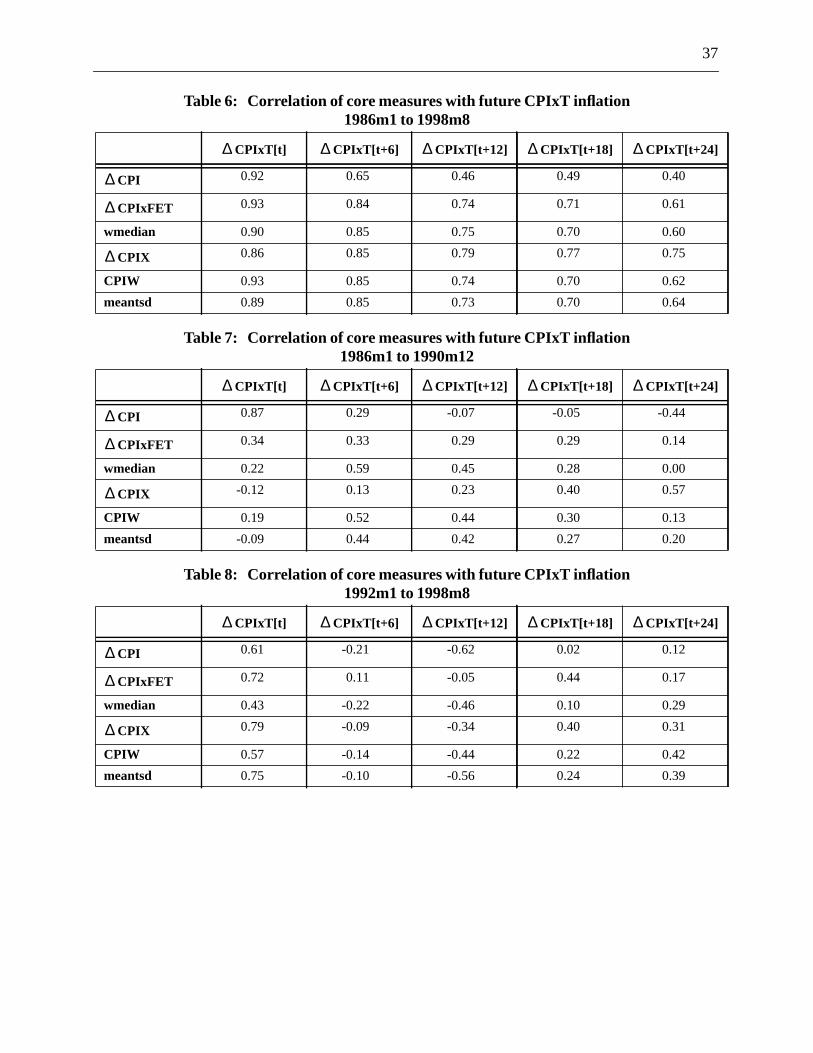
37

Table 6: Correlation of core measures with future CPIxT inflation1986m1 to 1998m8

Table 7: Correlation of core measures with future CPIxT inflation1986m1 to 1990m12

Table 8: Correlation of core measures with future CPIxT inflation1992m1 to 1998m8

CPIxT[t] CPIxT[t+6] CPIxT[t+12] CPIxT[t+18] CPIxT[t+24]

CPI 0.92 0.65 0.46 0.49 0.40

CPIxFET 0.93 0.84 0.74 0.71 0.61

wmedian 0.90 0.85 0.75 0.70 0.60

CPIX 0.86 0.85 0.79 0.77 0.75

CPIW 0.93 0.85 0.74 0.70 0.62

meantsd 0.89 0.85 0.73 0.70 0.64

CPIxT[t] CPIxT[t+6] CPIxT[t+12] CPIxT[t+18] CPIxT[t+24]

CPI 0.87 0.29 -0.07 -0.05 -0.44

CPIxFET 0.34 0.33 0.29 0.29 0.14

wmedian 0.22 0.59 0.45 0.28 0.00

CPIX -0.12 0.13 0.23 0.40 0.57

CPIW 0.19 0.52 0.44 0.30 0.13

meantsd -0.09 0.44 0.42 0.27 0.20

CPIxT[t] CPIxT[t+6] CPIxT[t+12] CPIxT[t+18] CPIxT[t+24]

CPI 0.61 -0.21 -0.62 0.02 0.12

CPIxFET 0.72 0.11 -0.05 0.44 0.17

wmedian 0.43 -0.22 -0.46 0.10 0.29

CPIX 0.79 -0.09 -0.34 0.40 0.31

CPIW 0.57 -0.14 -0.44 0.22 0.42

meantsd 0.75 -0.10 -0.56 0.24 0.39

∆ ∆ ∆ ∆ ∆

∆

∆

∆

∆ ∆ ∆ ∆ ∆

∆

∆

∆

∆ ∆ ∆ ∆ ∆

∆

∆

∆

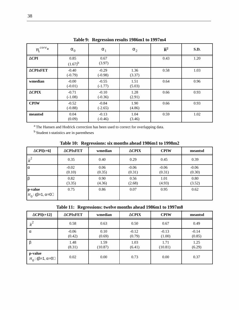
38

Table 9: Regression results 1986m1 to 1997m4

Table 10: Regressions: six months ahead 1986m1 to 1998m2

Table 11: Regressions: twelve months ahead 1986m1 to 1997m8

a

aThe Hansen and Hodrick correction has been used to correct for overlapping data.

R2 S.D.

∆CPI 0.85

(1.67)b

b Student t-statistics are in parentheses

0.67(3.97)

0.43 1.20

∆CPIxFET -0.40(-0.79)

-0.29(-0.98)

1.36(3.37)

0.58 1.03

wmedian -0.00(-0.01)

-0.55(-1.77)

1.51(5.03)

0.64 0.96

∆CPIX -0.71(-1.08)

-0.10(-0.36)

1.28(2.91)

0.66 0.93

CPIW -0.52(-0.88)

-0.84(-2.65)

1.90(4.86)

0.66 0.93

meantsd 0.04(0.09)

-0.13(-0.46)

1.04(3.46)

0.59 1.02

∆CPI[t+6] ∆CPIxFET wmedian ∆CPIX CPIW meantsd

0.35 0.40 0.29 0.45 0.39

α -0.02(0.10)

0.06(0.35)

-0.06(0.31)

-0.06(0.31)

-0.06(0.30)

β 0.82(3.35)

0.90(4.36)

0.56(2.68)

1.01(4.93)

0.80(3.52)

p-value: (β=1, α=0)

0.75 0.86 0.07 0.95 0.62

∆CPI[t+12] ∆CPIxFET wmedian ∆CPIX CPIW meantsd

0.58 0.63 0.50 0.67 0.49

α -0.06(0.42)

0.10(0.69)

-0.12(0.79)

-0.13(1.00)

-0.14(0.85)

β 1.48(8.31)

1.59(10.87)

1.03(6.41)

1.71(10.81)

1.25(6.29)

p-value: (β=1, α=0) 0.02 0.00 0.73 0.00 0.37

πtcore α0 α1 α2

R2

H0

R2

H0

39

Table 12: Regressions: eighteen months ahead 1986m1 to 1997m2

Table 13: Regressions: six months ahead 1992m1 to 1998m2

Table 14: Regressions: twelve months ahead 1992m1 to 1997m8

Table 15: Regressions: eighteen months ahead 1992m1 to 1997m2

∆CPI[t+18] ∆CPIxFET wmedian ∆CPIX CPIW meantsd

0.55 0.55 0.52 0.54 0.45

α -0.19(2.22)

-0.06(0.61)

-0.23(2.55)

-0.27(2.98)

-0.26(2.63)

β 1.39(13.07)

1.42(13.71)

1.01(11.75)

1.49(13.64)

1.16(10.10)

p-value: (β=1, α=0) 0.00 0.00 0.03 0.00 0.02

∆CPI[t+6] ∆CPIxFET wmedian ∆CPIX CPIW meantsd

0.29 0.29 0.26 0.32 0.20

α -0.23(1.25)

-0.12(0.55)

-0.41(3.22)

-0.26(1.37)

-0.23(1.19)

β 0.81(3.91)

0.96(6.57)

0.82(4.08)

1.00(5.80)

0.90(1.94)

p-value: (β=1, α=0)

0.44 0.79 0.36 0.98 0.48

∆CPI[t+12] ∆CPIxFET wmedian ∆CPIX CPIW meantsd

0.70 0.50 0.64 0.64 0.41

α -0.48(2.98)

-0.20(1.13)

-0.83(4.28)

-0.49(2.76)

-0.43(2.08)

β 1.63(11.60)

1.67(7.13)

1.67(11.99)

1.85(10.25)

1.70(5.21)

p-value: (β=1, α=0)

0.00 0.00 0.00 0.00 0.03

∆CPI[t+18] ∆CPIxFET wmedian ∆CPIX CPIW meantsd

0.66 0.34 0.60 0.46 0.44

α -0.47(4.83)

-0.20(1.67)

-0.73(6.11)

-0.43(3.66)

-0.42(3.55)

β 1.36(14.55)

1.17(7.33)

1.37(16.91)

1.34(12.06)

1.49(11.15)

p-value: (β=1, α=0)

0.00 0.14 0.00 0.00 0.00

R2

H0

R2

H0

R2

H0

R2

H0

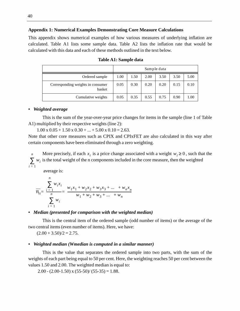
40

n areld be

Table

y after

t thed

of the

of theeen the

Appendix 1: Numerical Examples Demonstrating Core Measure Calculations

This appendix shows numerical examples of how various measures of underlying inflatiocalculated. Table A1 lists some sample data. Table A2 lists the inflation rate that woucalculated with this data and each of these methods outlined in the text below.

• Weighted average

This is the sum of the year-over-year price changes for items in the sample (line 1 ofA1) multiplied by their respective weights (line 2):

1.00 x 0.05 + 1.50 x 0.30 + ... + 5.00 x 0.10 = 2.63.Note that other core measures such as CPIX and CPIxFET are also calculated in this wacertain components have been eliminated through a zero weighting.

More precisely, if each is a price change associated with a weight , such thais the total weight of the n components included in the core measure, then the weighte

average is:

• Median (presented for comparison with the weighted median)

This is the central item of the ordered sample (odd number of items) or the averagetwo central items (even number of items). Here, we have:

(2.00 + 3.50)/2 = 2.75.

• Weighted median (Wmedian is computed in a similar manner)

This is the value that separates the ordered sample into two parts, with the sumweights of each part being equal to 50 per cent. Here, the weighting reaches 50 per cent betwvalues 1.50 and 2.00. The weighted median is equal to:

2.00 - (2.00-1.50) x (55-50)/ (55-35) = 1.88.

Table A1: Sample data

Sample data

Ordered sample 1.00 1.50 2.00 3.50 3.50 5.00

Corresponding weights in consumerbasket

0.05 0.30 0.20 0.20 0.15 0.10

Cumulative weights 0.05 0.35 0.55 0.75 0.90 1.00

xi wi 0≥wi

i 1=

n

∑

πit

wi xii 1=

n

∑

wii 1=

n

∑-------------------

w1x1 w2x2 w3x3 ... wnx+ n+ + +

w1 w2 w3 ... w+ n+ + +----------------------------------------------------------------------------------==

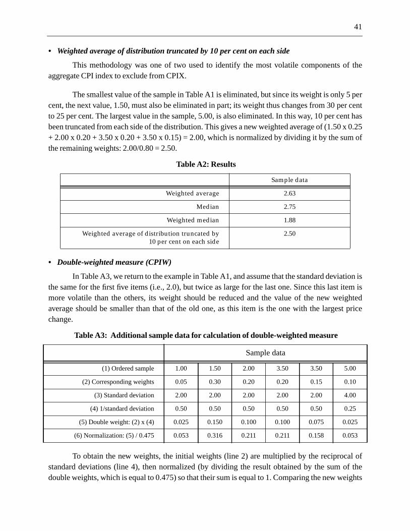
41

f the

perr centnt hasx 0.25

of

tion isem isightedt price

l off the

eights

• Weighted average of distribution truncated by 10 per cent on each side

This methodology was one of two used to identify the most volatile components oaggregate CPI index to exclude from CPIX.

The smallest value of the sample in Table A1 is eliminated, but since its weight is only 5cent, the next value, 1.50, must also be eliminated in part; its weight thus changes from 30 peto 25 per cent. The largest value in the sample, 5.00, is also eliminated. In this way, 10 per cebeen truncated from each side of the distribution. This gives a new weighted average of (1.50+ 2.00 x 0.20 + 3.50 x 0.20 + 3.50 x 0.15) = 2.00, which is normalized by dividing it by the sumthe remaining weights: 2.00/0.80 = 2.50.

• Double-weighted measure (CPIW)

In Table A3, we return to the example in Table A1, and assume that the standard deviathe same for the first five items (i.e., 2.0), but twice as large for the last one. Since this last itmore volatile than the others, its weight should be reduced and the value of the new weaverage should be smaller than that of the old one, as this item is the one with the largeschange.

To obtain the new weights, the initial weights (line 2) are multiplied by the reciprocastandard deviations (line 4), then normalized (by dividing the result obtained by the sum odouble weights, which is equal to 0.475) so that their sum is equal to 1. Comparing the new w

Table A2: Results

Sample data

Weighted average 2.63

Median 2.75

Weighted median 1.88

Weighted average of distribution truncated by

10 per cent on each side

2.50

Table A3: Additional sample data for calculation of double-weighted measure

Sample data

(1) Ordered sample 1.00 1.50 2.00 3.50 3.50 5.00

(2) Corresponding weights 0.05 0.30 0.20 0.20 0.15 0.10

(3) Standard deviation 2.00 2.00 2.00 2.00 2.00 4.00

(4) 1/standard deviation 0.50 0.50 0.50 0.50 0.50 0.25

(5) Double weight: (2) x (4) 0.025 0.150 0.100 0.100 0.075 0.025

(6) Normalization: (5) / 0.475 0.053 0.316 0.211 0.211 0.158 0.053

42

ationeased

53 =3.

puted

ightsyear-

so that

ent of

e) inn bee isPI. Fortion ofnce ofothertion ofent, a

with the initial weights, the weight of the last item is reduced by about half (its standard devibeing twice as high as that of the other items), while that of each of the first five items has incrslightly.

In this case, the new weighted average, 1.00 x 0.053 + 1.50 x 0.316 + ... + 5.00 x 0.02.50, is smaller than the one calculated with the conventional weights, which was equal to 2.6

For example, the double-weighted measure of core inflation, known as CPIW, is comas follows:

where is the double weight, computed as the product of the time-varying published wefor the components and the inverse of the standard deviation of the difference between theover-year inflation rate for each component and the total CPI. These weights are normalizedthey sum to one:17

where is the standard deviation, and

is calculated for the period between January 1986 and April 1997 as:

where represents the weighted mean of the year-over-year change in a particular compon

the CPI, and is the year-over-year change in the published CPI.

Table A4 lists the components whose weights changed the most (in absolute valumoving from total CPI to CPIW. It also shows the extent to which the component weights camodified as a function of the variability of their relative prices. The change in relative pricmeasured by the difference between the price change of the component and that of the total Cexample, the weight of the component whose relative price change is lowest (standard devia0.85), “Food purchased from restaurants,” rises from 5.40 per cent to 13.23 per cent, a differe7.83 percentage points. Its weight is 2.5 times higher in CPIW than in the total CPI. On thehand, the weight of the component whose relative price change is highest (standard devia16.32), “tobacco products and smokers’ supplies,” drops from 1.63 per cent to 0.21 per c

17. Note that the weights are time-varying owing to revisions in basket weights.

πtCPIW πit

i 1=

n

∑ dwti t•=

dwtit

dwtit

wi t,1σ---

i•

wi t,i 1=

n

∑ 1σ---

i•

-----------------------------------

= σi

σi

σi1

n 1–------------

πit πtCPI

–( ) πit πtCPI

–( )–[ ]∑2

=

12---

πit

πtCPI

43

eighth

re theich isdardtablefore,nd in

h andles and

difference of 1.42 percentage points. Its weight in CPIW amounts to no more than about one-of that assigned in the total CPI.

The components listed in Table A4 are not necessarily those whose relative prices amost volatile. For example, the relative price of “vegetable and vegetable preparations,” whnot included in the table, is much more volatile than the price of “other food products” (standeviation of 9.31 versus 3.39). However, the weight given to “vegetables and vegepreparations” in the CPI is smaller than that of “other food products” (1.06 versus 2.70). Therethe difference, in absolute terms, between the weights of the first component in the CPI aCPIW is smaller than that of the second component.

Table A4: Components whose weights have changed most in CPIW (in absolute value)

Component(1)

Weightin CPI

(2)Weight

in CPIW

(3)Difference(2) - (1)

(4)a

StandardDeviation

ofDifference

aThe standard deviation is calculated for the period between January 1986 and April 1997.

Ratio(2)/(1)

Food purchased from restaurants 5.40 13.23 7.83 0.85 2.5

Rented accommodation 7.18 14.65 7.47 1.02 2.0

Clothing 4.16 5.55 1.39 1.56 1.3

Purchase of automotive vehicles 7.47 4.15 -3.22 3.64 0.6

Mortgage interest cost 5.33 2.36 -2.97 4.68 0.4

Gasoline 3.81 0.86 -2.95 9.14 0.2

Property replacement cost 3.29 1.23 -2.06 5.54 0.4

Tobacco products & smokers’ supplies 1.63 0.21 -1.42 16.32 0.1

Meat 3.04 1.73 -1.31 3.65 0.6

Other food productsb

b Residual item of the food category of our 54-component set. The food category includes the following items: meat; fisother seafood; dairy products and eggs; bakery and other cereal products; fruits, fruit preparations, and nuts; vegetabvegetable preparations; food purchased from restaurants; and other food products.

2.70 1.65 -1.05 3.39 0.6

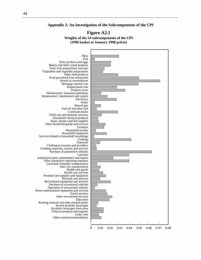
44

Appendix 2: An Investigation of the Subcomponents of the CPI

Other owned accommodationLease, rent

Tobacco products and suppliesAlcoholic beverages from store

Served alcoholic beveragesReading material and other printed matter

EducationOther recreational services

Travel servicesHome entertainment equipment and services

Operation of recreational vehiclesPurchase of recreational vehicles

Recreational equipment and servicesPersonal care services

Personal care supplies and equipmentHealth care services

Health care goodsInter-city transportation

Local and commuter transportationOther automotive operating expenses

Automotive parts, maintenance and repairsGasoline

Purchase of automotive vehiclesClothing materials, notions and services

Clothing accessories and jewelleryFootwearClothing

Services related to household furnishingsHousehold equipment

Household textilesFurniture

Other household goods and servicesPaper, plastics and foil supplies

Household chemical productsChild care and domestic services

CommunicationsFuel oil and other fuel

Natural gasWater

ElectricityHomeowners’ maintenance and repairs

Replacement costMortgage interest cost

Rented accommodationFood purchased from restaurants

Other food productsVegetables and vegetable preparations

Fruit, fruit preparations and nuts

Homeowners’ insurance premiumsProperty taxes

Bakery and other cereal productsDairy products and eggs

FishMeat

Figure A2.1Weights of the 54 subcomponents of the CPI

(1996 basket at January 1998 prices)

0 0.01 0.02 0.03 0.04 0.05 0.06 0.07 0.08

45

59

.70

6

.37

57

22

6

.93

83

6

.60

.31

.05

.09

2

98

39

7

3

.72

.10

01

Table A2.1: Year-over-year growth of the 54 subcomponents of the CPI

Full sample86m1 to 98m8

Subsample86m1 to 91m12

Subsample92m1 to 98m8

Component1996Wt.

MeanStd.

Deva MeanStd.Dev

MeanStd.Dev

Meat 0.0290 2.64 3.85 4.20 4.47 1.21 2.48

Fish 0.0041 3.24 3.61 4.74 3.94 1.88 2.64

Dairy products and eggs 0.0208 2.10 1.61 2.84 1.29 1.44 1.

Bakery and other cereal products 0.0204 2.71 1.69 3.32 1.46 2.16 1

Fruit, fruit preparations and nuts 0.0140 1.26 5.23 3.96 5.23 -1.17 3.89

Vegetables and veg. preparations 0.0125 2.56 9.64 4.68 10.08 0.65 8.85

Other food products 0.0282 1.72 3.00 2.24 2.61 1.25 3.2

Food purchased from restaurants 0.0498 3.06 1.57 4.60 0.74 1.67 0

Rented accommodation 0.0717 2.78 1.31 4.02 0.59 1.67 0.

Mortgage interest cost 0.0491 0.94 6.02 5.42 5.04 -3.10 3.41

Replacement cost 0.0268 3.12 5.58 6.26 6.75 0.29 1.

Property taxes 0.0355 4.78 2.59 6.61 1.05 3.14 2.4

Homeowners’ insurance prems. 0.0105 4.09 4.96 6.52 6.06 1.91 1

Homeowners’ maint. & repairs 0.0169 1.65 2.56 2.83 1.55 0.59 2.

Electricity 0.0265 3.42 2.47 4.87 1.63 2.10 2.37

Water 0.0039 5.14 2.73 6.12 3.04 4.25 2.06

Natural gas 0.0102 0.78 5.46 -1.68 3.45 3.00 5.97

Fuel oil and other fuel 0.0058 0.55 11.49 0.68 15.24 0.43 6.61

Communications 0.0279 0.88 2.62 -0.68 2.29 2.28 2.0

Child care and domestic services 0.0110 4.37 2.02 5.87 1.23 3.02 1

Household chemical products 0.0073 1.51 2.76 3.58 1.44 -0.36 2

Paper, plastics and foil supplies 0.0079 2.88 4.73 3.56 2.46 2.26 6

Other household goods&serv. 0.0148 2.78 2.36 4.99 1.03 0.78 1

Furniture 0.0137 1.82 1.99 3.17 1.62 0.60 1.44

Household textiles 0.0052 1.55 2.65 3.22 2.13 0.05 2.1

Household equipment 0.0164 1.08 1.69 2.17 1.64 0.10 0.

Services rel. to hh furnishings 0.0033 3.26 1.73 4.51 1.10 2.13 1.

Clothing 0.0417 2.01 1.83 3.45 1.38 0.72 1.07

Footwear 0.0093 1.85 1.93 3.30 1.32 0.53 1.3

Clothing accs. & jewellery 0.0055 1.40 2.50 3.37 1.44 -0.38 1.8

Clothing mat., notions and ser. 0.0059 2.92 1.57 4.42 0.60 1.58 0

Purchase of automotive vehicles 0.0630 3.96 2.75 3.77 3.33 4.12 2

Gasoline 0.0393 0.89 9.07 1.88 11.81 -0.01 5.51

Auto. parts, maint. & repairs 0.0230 2.05 2.17 3.68 1.94 0.58 1.

46

.68

36

25

20

.00

.99

.81

.34

.55

.68

0

.09

1

11

.86

55

9

.23

Other auto operating expenses 0.0398 6.32 2.67 7.42 2.21 5.32 2

Local & commuter transport. 0.0063 5.45 2.88 6.60 1.58 4.41 3.

Inter-city transportation 0.0100 6.58 8.90 6.99 11.73 6.21 5.23

Health care goods 0.0085 3.98 3.69 7.29 2.46 0.99 1.

Heath care services 0.0126 3.43 1.47 4.63 0.42 2.35 1.

Personal care supplies & equip. 0.0155 1.53 2.04 2.71 1.32 0.46 2

Personal care services 0.0095 3.79 1.97 5.53 1.16 2.23 0

Recreational equip.& services 0.0206 0.45 2.94 2.81 2.02 -1.66 1

Purchase of recreational vehicles 0.0067 4.11 2.22 4.67 2.80 3.60 1

Operation of recreational vehicles 0.0041 3.41 3.37 5.54 3.56 1.49 1

Home entertain. equip. & services 0.0156 -0.55 1.98 0.35 1.90 -1.35 1

Travel services 0.0169 3.48 3.67 3.93 2.93 3.08 4.2

Other recreational services 0.0220 5.09 1.97 6.68 1.42 3.65 1

Education 0.0192 7.48 2.83 7.45 3.61 7.51 1.9

Reading mat. & oth. print. matter 0.0075 4.50 2.31 6.04 1.35 3.11 2.

Served alcoholic beverages 0.0058 3.96 3.05 6.82 1.78 1.39 0

Alcoholic beverages from store 0.0130 3.97 2.55 6.02 1.73 2.12 1.

Tobacco products & supplies 0.0130 8.91 11.17 16.35 9.82 2.21 7.49

Lease rent 0.0082 2.48 5.09 3.47 4.95 1.59 5.0

Other owned accommodation 0.0107 3.42 3.12 6.14 2.15 0.96 1

All-items CPI 1.0000 2.96 1.77 4.66 0.73 1.43 0.72aThis is the standard deviation of the inflation rate for the individual component.

Table A2.1: Year-over-year growth of the 54 subcomponents of the CPI

Full sample86m1 to 98m8

Subsample86m1 to 91m12

Subsample92m1 to 98m8

Component1996Wt.

MeanStd.

Deva MeanStd.Dev

MeanStd.Dev

47

Table A2.2: Frequency of elimination of the CPI components in the calculation ofmeantsd (1986m1 to 1998m8)

Component meantsd

# %

Vegetables and vegetable preparations 76 50

Inter-city transportation 74 49

Natural gas 72 47

Fuel oil and other fuel 70 46

Gasoline 69 45

Education 54 36

Tobacco products and smokers’ supplies 53 35

Mortgage interest cost 51 34

Fruit, fruit preparation, and nuts 38 25

Rental and leasing of automotive vehicles 27 18

Communications 26 17

Replacement cost 26 17

Homeowners’ insurance premiums 24 16

Recreational equipment and services 17 11

Other automotive vehicle operating expenses 17 11

Fish and other seafood 17 11

Local and commuter transportation 16 11

Travel services 16 11

Paper, plastics, and foil supplies 15 10

Water 14 9

Home-entertainment equipment and services 13 9

Health-care goods 12 8

Property taxes 12 8

Other food products 9 6

Homeowners’ maintenance and repairs 7 5

Reading material and other printed matter 7 5

Household textiles 6 4

Clothing accessories and jewellery 5 3

Personal-care supplies and equipment 5 3

Meat 4 3

Other recreational services 3 2

Electricity 2 1

Household chemical products 2 1

Child care and domestic services 2 1

Operation of recreational vehicles 2 1

Other owned accommodation expenses 1 0

Furniture 1 0

Footwear 1 0

Purchase of recreational vehicles 1 0

Served alcoholic beverages 1 0

48

Table A2.3: Frequency of elimination of the CPI components in the calculation ofmeantsd (1992m1 to 1998m8)

Component meantsd

# %

Education 44 55

Mortgage interest cost 36 45

Vegetables and vegetable preparation 35 44

Natural gas 34 43

Inter-city transportation 30 38

Gasoline 24 30

Fuel oil and other fuel 24 30

Tobacco products and smokers’ supplies 22 28

Fruit, fruit preparations and nuts 21 26

Rental and leasing of automotive vehicles 18 23

Recreational equipment and services 17 21

Travel services 16 20

Other automotive vehicles operating expenses 16 20

Local and commuter transportation 16 20

Paper, plastics, and foil supplies 15 19

Water 12 15

Property taxes 12 15

Home-entertainment equipment and services 10 13

Other food products 8 10

Homeowners’ maintenance and repairs 7 9

Fish and other seafood 7 9

Reading material and other printed matter 7 9

Household textiles 5 6

Clothing accessories and jewellery 5 6

Personal-care supplies and equipment 5 6

Electricity 2 3

Communications 2 3

Child care and domestic services 2 3

Household chemical products 2 3

Homeowner’s insurance premium 1 1

Furniture 1 1

Footwear 1 1

Purchase of recreational vehicles 1 1

Other recreational services 1 1

49

Table A2.4: Frequency of elimination of the CPI components in the calculation ofmeantsd (1996m12 to 1998m8)

Components meantsd

# %

Fuel oil and other fuel 19 91

Inter-city transportation 19 91

Mortgage interest cost 18 86

Education 17 81

Natural gas 14 67

Gasoline 13 62

Vegetables and vegetable preparations 10 48

Home entertainment equipment and services 8 38

Other automotive vehicle operating expenses 7 33

Travel services 6 29

Tobacco 5 24

Fruit, fruit preparations and nuts 2 10

Communications 1 5

Clothing accessories and jewellery 1 5

Rental and leasing of automotive vehicles 1 5

50

asure997)s andnessust ands andt theer, thee.

adianple. Foronth

sise into

igurescally.e alsos forurtosis

th ratesowthearlyto the

cienttosis,obustas the

samplea back

Appendix 3: An Investigation of the Skewness and Kurtosis

The moments of the distribution of price changes have implications for the methodology to mecore inflation. Bryan and Cecchetti (1993b, 1996) and Bryan, Cecchetti, and Wiggins II (1offer evidence that the population of monthly price changes is characterized by skewneskurtosis in the United States. Roger (1997) offers similar evidence for New Zealand. This skewand kurtosis suggests the choice of an order statistic, such as the weighted median, as a robefficient estimator of the central tendency in prices. In this appendix, we report the skewneskurtosis of the distribution of price changes for the Canadian CPI. Not surprisingly, we find thaprice change distributions for Canada are characterized by skewness and kurtosis. Howevextent of the skewness and kurtosis depends on the horizon used to calculate the price chang

Tables A3.1–A3.4 provide summary statistics on the skewness and kurtosis in the Candata. To show how these calculations are made, we take the year-over-year case as an exameach month from 1986m1 to 1998m8, we create a cross-sectional distribution of the 12th-mprice changes of each of 54 subindexes of the CPI.18 Then, we calculate the skewness and kurtoof each of the monthly distributions. As suggested by Roger (2000), these statistics takaccount the implicit weights that were actually used each month in the calculation of the CPI.19Theresulting measures of weighted skewness and weighted kurtosis are listed in Table A3.1. FA3.1 to A3.5 illustrate the time series of the skewness and kurtosis coefficients graphiAlthough the discussion in this appendix focuses exclusively on the weighted measures, wreport the more traditional, equally weighted, measures of the third and fourth momentcomparative purposes (see Table A3.2). Both methods of calculating skewness and kproduce statistics that suggest similar conclusions.

A3.1 Kurtosis

For the Canadian data, it appears that kurtosis depends on the frequency over which the groware calculated. Below the year-over-year horizon, kurtosis is very large (22.02 for monthly grrates, 17.57 for quarterly changes). At longer horizons, kurtosis is much lower (7.82 for ygrowth rates, 6.31 for 36-month changes), but remains at problematic levels when comparedkurtosis of 3 that corresponds to a normal distribution.

If a distribution is approximately normal, then the sample mean is an unbiased and effiestimator of the population mean. However, the efficiency is sensitive to kurtosis. High kurand in particular, a leptokurtic distribution indicate that the mean is a less-efficient and less-restimator of the population or underlying mean price change than an order statistic such

18. We use 54 subindexes because disaggregation at this level provided us with the longestpossible. Changes to the prices surveyed and to the basket made it difficult to extend the datfurther.

19. See footnote 9.

51

r pricensiderion, as

nthlyorizon.s. Onr-yearewness

ediant for thee data.monthdian isightedht bees thattion isably.” Hent andrage attistic to

re. Asonthlyeightedo 0.17urtosis

anadianlematic13.34

median. Canadian measures of core inflation are based on the distribution of year-over-yeachanges. At a year-over-year frequency, kurtosis averages 7.82; therefore, it is important to cothe weighted median as a robust estimator of the underlying population mean and, by extensa prospective measure of core inflation.

A3.2 Skewness

Skewness also varies with the frequency over which it is calculated. Seasonality in the mochanges will contribute to skewness in the data when price changes are calculated over this hAs the horizon becomes longer, from a monthly to quarterly to yearly basis, skewness fallaverage, skewness does not seem to present a major problem for distribution of year-ovechanges, where the average weighted skewness is 0.15. For longer horizons, however, skincreases again.

At the top of each of Figures A1–A5, we graph the weighted mean and the weighted mof the Canadian data to emphasize the problem that might be created by skewness. Note thamonth-over-month data, the weighted median seems to capture the central tendency of thThis also appears to be the case for the 3-month-over-3-month and 12-month-over-12-changes in the CPI. However, for the 24-month-over-24-month changes, the weighted meincreasingly below the weighted mean. In the 36-month-over-36-month changes, the wemedian consistently underpredicts the weighted mean. This demonstrates how it migmisleading to focus on a weighted median in the presence of skewness. Roger (1997) concludalthough the median is the most robust estimator, it is a biased estimator when the populaskewed. Roger finds that “slightly higher percentile of the price change distribution relicorrects for the asymmetry of the distribution, while maintaining its efficiency and robustnesstherefore calculates an alternative order statistic (the 57th percentile) as the most efficierobust estimator for New Zealand. However, since skewness is not a major problem on avethe year-over-year frequency, there seems to be no need to calculate an alternative order stathe 50th percentile for Canada, as Roger proposes for New Zealand.

A3.3 Seasonal adjustment

We also seasonally adjust the individual price change series using the ARIMA-X11 procedushown in Table A3.3, this reduces both the weighted skewness and weighted kurtosis in the mand quarterly changes. Seasonal adjustment of the individual price changes reduces the wskewness for the 1986–98 period from 0.36 to 0.19 for the monthly changes and from 0.33 tfor the quarterly changes. This supports the view that some of the observed skewness and kreflects seasonality in price changes. Thus, weighted skewness may not characterize the Cdata even at these higher frequencies. Kurtosis is also reduced although it remains at problevels. Kurtosis is 19.41 for monthly changes, compared to 22.02 in the unadjusted data, andfor quarterly changes, compared to 17.57 in the unadjusted data.

52

cross-thishey find

n theuggestis asthat

ts ofess ofoodheirias.

ess ins falleny 1992e firstmean

ngly,ugh itss and

thatation

low-. Thelting

A3.4 Changes in the skewness in the Canadian data in the low-inflation period

Ball and Mankiw (1995) argue that in the presence of menu costs, the skewness of thesectional distribution of price changes will be a predictor of inflation. Ball and Mankiw testhypothesis by examining the correlation between the sample mean and sample skewness. Tevidence consistent with their theory.

Bryan and Cecchetti (1996) challenge the existence of this positive correlation betweemean and skewness in the distribution of price changes. Their Monte Carlo experiments sthat this positive correlation is actually due to a large positive small-sample bias. The intuitionfollows. If we have a random draw from a symmetric distribution with mean zero, then drawsdeviate from the population mean of the distribution will affect both the first and third momenthe distribution, leading to a correlation between the moments. They suggest that the thicknthe tails of the probability distribution from which the draws are taken will determine the likelihof an extreme draw.20 Therefore, the kurtosis determines the size of the small-sample bias. TMonte Carlo experiments suggest that kurtosis above 4 results in a significant small-sample b

We do observe a positive correlation between the mean and the weighted skewnCanadian data. In recent years, the weighted mean of the year-over-year price changes hafrom 4.4 per cent for the January 1986 to December 1991 period to 1.6 per cent for the Januarto August 1998 period. At the same time, the average weighted skewness fell from 0.32 in thperiod to 0.00 in the second period (see Table A3.4). The correlation between the weightedand weighted skewness in inflation is quite evident in Figure A3, for example. Interestiweighted kurtosis has also fallen from 9.72 in the first period to 6.11 in the second period, thoremains problematic. Moreover, there is much less variation in the measures of skewnekurtosis (both weighted and unweighted) in the recent period of low inflation, suggestingskewness and kurtosis may reach problematic levels less often in the current low-inflenvironment.

The dramatic decline in weighted skewness and weighted kurtosis in the recentinflation period would suggest that there is no one underlying population of price changesdistribution of price changes is evolving over time with the policy environment and the resuinflation process.

20. If you increased the variance of a normal distribution you would get the same result.

53

Table A3.1: Summary statistics for price change distributions of various horizonsSample 86m1 to 98m8

Table A3.2: Summary statistics for price change distributionsEqually weighted price changes: Sample 86m1 to 98m8

Table A3.3: Summary statistics for price change distributionsSeasonally adjusted data & weights varied

Sample 1986m1 to 1998m8

Table A3.4: Summary statistics for 12M/12M price change distributions

M/M 3M/3M 12M/12M 24M/24M 36M/36M

Weighted SkewnessAverage 0.36 0.33 0.15 0.59 0.96

Std. dev 3.27 2.71 1.44 0.93 1.03

Weighted KurtosisAverage 22.02 17.57 7.82 6.17 6.31

Std. dev 15.67 12.08 4.19 2.94 4.28

M/M 3M/3M 12M/12M 24M/24M 36M/36M

SkewnessAverage 0.29 0.25 0.19 0.46 0.74

Std. dev 2.73 2.27 1.31 0.79 0.89

KurtosisAverage 15.99 13.48 7.31 5.58 5.69

Std. dev 9.45 7.18 3.76 2.23 3.76

M/M 3M/3M

Weighted MeanAverage 0.22 0.69

Std. dev 0.19 0.45

Weighted SkewnessAverage 0.19 0.17

Std. dev 3.13 2.35

Weighted KurtosisAverage 19.41 13.34

Std. dev 15.87 10.71

1986m1 to 1991m12 92m1 to 98m8

weighted meanAverage 4.40 1.60

Std. dev 0.66 0.49

Unweighted Weighted Unweighted WeightedSkewness

Average 0.07 0.32 0.30 0.00

Std. dev 1.76 1.93 0.68 0.75

KurtosisAverage 9.04 9.72 5.75 6.11

Std. dev 4.23 4.42 2.40 3.12

54

98

98

98

Figure A3.1: Month-over-month changes

1986 1987 1988 1989 1990 1991 1992 1993 1994 1995 1996 1997 19-1

0

1

2

weighted meanweighted median

Weighted Mean vs Weighted MedianMonth over month growth of CPI, monthly data

Jan. 1986 to Aug. 1998

1986 1987 1988 1989 1990 1991 1992 1993 1994 1995 1996 1997 19-10

-5

0

5

10

Skewness over sampleMonth over month growth of CPI, monthly data

Jan. 1986 to Aug. 1998

1986 1987 1988 1989 1990 1991 1992 1993 1994 1995 1996 1997 190

20

40

60

80

Kurtosis over sampleMonth over month growth of CPI, monthly data

Jan. 1986 to Aug. 1998

55

98

98

98

Figure A3.2: Quarter-over-quarter changes

1986 1987 1988 1989 1990 1991 1992 1993 1994 1995 1996 1997 19

0

2

weighted meanweighted median

Weighted Mean vs Weighted MedianQuarter over quarter growth of CPI, monthly data

Jan. 1986 to Aug. 1998

1986 1987 1988 1989 1990 1991 1992 1993 1994 1995 1996 1997 19-10

-5

0

5

10

Skewness over sampleQuarter over quarter growth of CPI, monthly data

Jan. 1986 to Aug. 1998

1986 1987 1988 1989 1990 1991 1992 1993 1994 1995 1996 1997 190

20

40

60

80

Kurtosis over sampleQuarter over quarter growth of CPI, monthly data

Jan. 1986 to Aug. 1998

56

98

98

98

Figure A3.3: Year-over-year changes

1986 1987 1988 1989 1990 1991 1992 1993 1994 1995 1996 1997 190

2

4

6

weighted meanweighted median

Weighted Mean vs Weighted MedianYear over year growth of CPI, monthly data

Jan. 1986 to Aug. 1998

1986 1987 1988 1989 1990 1991 1992 1993 1994 1995 1996 1997 19-4

-2

0

2

4

Skewness over sampleYear over year growth of CPI, monthly data

Jan 1986 to Apr 1998

1986 1987 1988 1989 1990 1991 1992 1993 1994 1995 1996 1997 190

10

20

Kurtosis over sampleYear over year growth of CPI, monthly data

Jan 1986 to Apr 1998

57

98

98

98

Figure A3.4: 24-month-over-24-month changes

1986 1987 1988 1989 1990 1991 1992 1993 1994 1995 1996 1997 190

5

10

15

weighted meanweighted median

Weighted Mean vs Weighted Median24 months over 24 months growth of CPI, monthly data

Jan. 1986 to Aug. 1998

1986 1987 1988 1989 1990 1991 1992 1993 1994 1995 1996 1997 19-2

0

2

4

Skewness over sample24 months over 24 months growth of CPI, monthly data

Jan. 1986 to Aug. 1998

1986 1987 1988 1989 1990 1991 1992 1993 1994 1995 1996 1997 190

5

10

15

Kurtosis over sample24 months over 24 months growth of CPI, monthly data

Jan. 1986 to Aug. 1998

58

98

98

98

Figure A3.5: 36-month-over-36-month changes

1986 1987 1988 1989 1990 1991 1992 1993 1994 1995 1996 1997 190

10

20

weighted meanweighted median

Weighted Mean vs Weighted Median36 months over 36 months growth of CPI, monthly data

Jan. 1986 to Aug. 1998

1986 1987 1988 1989 1990 1991 1992 1993 1994 1995 1996 1997 19-2

0

2

4

Skewness over sample36 months over 36 months growth of CPI, monthly data

Jan. 1986 to Aug. 1998

1986 1987 1988 1989 1990 1991 1992 1993 1994 1995 1996 1997 190

5

10

15

20

Kurtosis over sample36 months over 36 months growth of CPI, monthly data

Jan 1986 to Apr 1998

Bank of Canada Technical ReportsRapports techniques de la Banque du Canada

Technical reports are generally published in the language of the author, with an abstract in both official languages.Les rapports techniques sont publiés généralement dans la langue utilisée par les auteurs; ils sont cependant précédésd’un résumé bilingue.

2000

88 International Financial Crises and Flexible Exchange Rates: Some Policy J. Murray, M. Zelmer,

Lessons from Canada and Z. Antia

1999

87 The Regulation of Central Securities Depositories and the Linkages between

CSDs and Large-Value Payment Systems C. Freedman

86 Greater Transparency in Monetary Policy: Impact on Financial Markets P. Muller and M. Zelmer

85 Inflation Targeting under Uncertainty G. Srour

84 Yield Curve Modelling at the Bank of Canada D. Bolder and D. Stréliski

1998

83 The Benefits of Low Inflation: Taking Stock B. O’Reilly

82 The Financial Services Sector: Past Changes and Future Prospects C. Freedman and C. Goodlet

81 The Canadian Banking System C. Freedman

1997

80 Constraints on the Conduct of Canadian Monetary Policy in the 1990s:

Dealing with Uncertainty in Financial Markets K. Clinton and M. Zelmer

79 Measurement of the Output Gap: A Discussion of Recent Research at

the Bank of Canada P. St-Amant and S. van Norden

1996

78 Do Mechanical Filters Provide a Good Approximation of Business Cycles? A. Guay and P. St-Amant

77 A Semi-Structural Method to Estimate Potential Output:

Combining Economic Theory with a Time-Series Filter

The Bank of Canada’s New Quarterly Projection Model, Part 4 L. Butler

76 Excess Volatility and Speculative Bubbles in the Canadian Dollar: J. Murray, S. van Norden,

Real or Imagined? and R. Vigfusson

75 The Dynamic Model: QPM, The Bank of Canada’s D. Coletti, B. Hunt,

New Quarterly Projection Model, Part 3 D. Rose, and R. Tetlow

74 The Electronic Purse: An Overview of Recent Developments and Policy Issues G. Stuber

Copies of the above titles and a complete list of Bank of Canada technical reports are available from:Pour obtenir des exemplaires des rapports susmentionnés et une liste complète des rapports techniques de la Banque du Canada,prière de s’adresser à :

Publications Distribution, Bank of Canada Diffusion des publications, Banque du Canada

234 Wellington Street, Ottawa, Ontario K1A 0G9 234, rue Wellington, Ottawa (Ontario) K1A 0G9

E-mail/Adresse électronique: publications@bankofcanada.ca

Web site: www.bankofcanada.ca