copyright warning & restrictionsarchives.njit.edu/vol01/etd/2000s/2005/njit-etd2005-038/...nh...
TRANSCRIPT

Copyright Warning & Restrictions
The copyright law of the United States (Title 17, United States Code) governs the making of photocopies or other
reproductions of copyrighted material.
Under certain conditions specified in the law, libraries and archives are authorized to furnish a photocopy or other
reproduction. One of these specified conditions is that the photocopy or reproduction is not to be “used for any
purpose other than private study, scholarship, or research.” If a, user makes a request for, or later uses, a photocopy or reproduction for purposes in excess of “fair use” that user
may be liable for copyright infringement,
This institution reserves the right to refuse to accept a copying order if, in its judgment, fulfillment of the order
would involve violation of copyright law.
Please Note: The author retains the copyright while the New Jersey Institute of Technology reserves the right to
distribute this thesis or dissertation
Printing note: If you do not wish to print this page, then select “Pages from: first page # to: last page #” on the print dialog screen

The Van Houten library has removed some ofthe personal information and all signatures fromthe approval page and biographical sketches oftheses and dissertations in order to protect theidentity of NJIT graduates and faculty.
ABSTRACT
BUS ARRIVAL TIME PREDICTION USING STOCHASTICTIME SERIES AND MARKOV CHAINS
byRajat Rajbhandari
Public transit agencies rely on disseminating accurate and reliable information to transit
users to achieve higher service quality and attract more users. With the development of
new technologies, the concept of providing users with reliable information about bus
arrival times at bus stops has become increasingly attractive. Due to the fact that bus
operation parameters and variables are highly stochastic, modeling prediction of bus
travel and arrival times has become one of the many challenging tasks.
Stochastic time series and delay propagation models to predict bus arrival times
using historical information were developed. Markov models were developed to predict
propagation of bus delay to downstream bus stops based on heterogeneous conditions.
The bus arrival times were predicted using a Markov model only and performance
measures were obtained and a combined arrival time prediction model consisting of delay
propagation and full autoregressive model was also developed. The inclusion of bus
delay propagation into the bus arrival time prediction algorithm is an important
contribution to the research efforts to predict bus arrival times. The research showed that
Markov models can provide accurate bus arrival time predictions without increasing the
need for a large number of bus operation variables, simulations and high polling
frequency of the geographical bus location as used by other modeling approaches.

BUS ARRIVAL TIME PREDICTION USING STOCHASTICTIME SERIES AND MARKOV CHAINS
byRajat Rajbhandari
A DissertationSubmitted to the Faculty of
New Jersey Institute of TechnologyIn Partial Fulfillment of the Requirements for the Degree of
Doctor of Philosophy in Transportation
Interdisciplinary Program in Transportation
January 2005

Copyright © 2005 by Rajat Rajbhandari
ALL RIGHTS RESERVED

APPROVAL PAGE
BUS ARRIVAL TIME PREDICTION USING STOCHASTICTIME SERIES AND MARKOV CHAINS
Rajat Rajbhandari
Dr. Janice Daniel, Dissertation AdvisorAssociate Professor of Civil EngineeringDepartment of Civil and Environmental Engineering, NJIT
Dr. Athanassios &Maas, Committee MemberAssociate Professor of Industrial EngineeringDirector, Interdisciplinary Program in Transportation, NJIT
DryLazar Spasdvic, Committee MemberProfessor of Civil EngineeringDirector, National Center for Transportation and Industrial Productivity, NJIT
Dr. Rathel-Ettrrommittee MemberAssistant Professor of Civil EngineeringDepartment of Civil and Environmental Engineering, NJIT
Date
Date
Date
Date
Dr. Stevtn Chien, Committee Member Date
Associate Professor of Civil EngineeringDepartment of Civil and Environmental Engineering, NJIT

BIOGRAPHICAL SKETCH
Author: Rajat Rajbhandari
Degree: Doctor of Philosophy
Date: January 2005
Undergraduate and Graduate Education:
• Doctor of Philosophy in Transportation,New Jersey Institute of Technology, Newark, NJ, 2005
• Master of Science in Civil Engineering,New Jersey Institute of Technology, Newark, NJ, 2002
• Bachelors in Civil Engineering,Tribhuwan University, Kathmandu, 1997
Major: Transportation
Presentations and Publications:
Rajat Rajbhandari and Janice Daniel,"Imioacts of the 65-mph Speed Limit on Truck Safety,"82na Annual Meeting of Transportation Research Board, Washington D.C.,January 2003.
Rajat Rajbhandari, Steven Chien and Janice Daniel,"Estimation of Bus Dwell Time using Automatic Passenger CounterInformation," Transportation Research Record 1841, Transportation ResearchBoard, 2003.
Janice Daniel and Rajat Rajbhandari,"Identifying Locations for Bus Nub Installations on Urban Roadways,"Urban Street Symposium, California, 2003.
iv

This dissertation is dedicated to my sweet wife, my loving parents, a wonderful sisterand many friends.
v
ACKNOWLEDGEMENT
Sincere gratitude goes to Dr. Janice Daniel, who guided me ever since I was a master's
student, with whom I had the privilege of working in numerous research projects and
who was my thesis and dissertation advisor. Her constant encouragement has been highly
valuable to me during my entire graduate studies. My appreciation also goes to
Dr. Steven Chien, Dr. Athanassios Bladikas, Dr. Lazar Spasovic and Dr. Rachel Liu for
being on my dissertation committee, and providing me with valuable comments.
Without the financial support of Department of Civil Engineering and National
Center for Transportation and Industrial Productivity at NJIT, I would not have been able
to complete my graduate studies.
Finally, many thanks to amazing friends at NJIT — Xiaobo Liu, Renu Chhonkar,
Chuck Tsai, Arun Raj. I am also thankful to my friends outside NJIT - Anil Tuladhar,
Anish Pradhan and Ramesh Byanjankar for their moral help and support. Finally, I'm
indebted to my wife, Reema, who constantly encouraged me to run when I would be
otherwise dragging my feet.
vi
TABLE OF CONTENTS
Chapter Page
1 INTRODUCTION 1
1.1 Introduction 1
1.2 Problem Statement 2
1.3 Research Objectives 3
1.4 Organization of the Dissertation 4
2 LITERATURE REVIEW 5
2.1 Introduction 5
2.2 Applications of Bus Arrival Prediction Models 5
2.3 Data Source and Errors 6
2.4 Bus Arrival Time Prediction Models 8
2.4.1 Time-Distance Model 8
2.4.2 Regression Models 10
2.4.3 Artificial Neural Network Models 12
2.4.4 Kalman Filter Models 13
2.5 Bus Delay Propagation 15
2.5.1 Delay Propagation Models 15
2.5.2 Finite State Markov Chains 17
2.6 Stochastic Time Series Models 18
2.6.1 Stochastic Models for Traffic Prediction 18
2.6.2 Comparison of ARIMA Models 21
2.7 Summary 22
vii
TABLE OF CONTENTS(Continued)
Chapter Page
3 ALGORITHM AND METHODOLOGY 25
3.1 Introduction 25
3.2 Assumptions and Constraints 25
3.3 Bus Arrival Time Prediction Algorithms 27
3.3.1 Delay Propagation Model 27
3.3.2 Travel Time and Delay Propagation Model 31
3.4 Selection of Travel Time Prediction Models 35
3.4.1 Box-Jenkins Approach 35
3.4.2 Autocorrelation and Partial Autocorrelation Functions 35
3.4.3 Optimal Order of AR Model 38
3.5 Stochastic Travel Time Models 39
3.5.1 Historical Average and Exponential Filter Models 39
3.5.2 Autoregressive and Moving Average Models 41
3.5.3 ARIMA Models 43
3.5.4 Subset ARIMA Models 44
3.5.5 Residual Analysis and Performance of Models 46
3.6 Discrete and Finite State Delay Propagation Model 47
3.6.1 Finite State Markov Chain 47
3.6.2 Estimation of Transition Probabilities 51
3.6.3 Application of Markov Chain to Predict Delay 52
viii
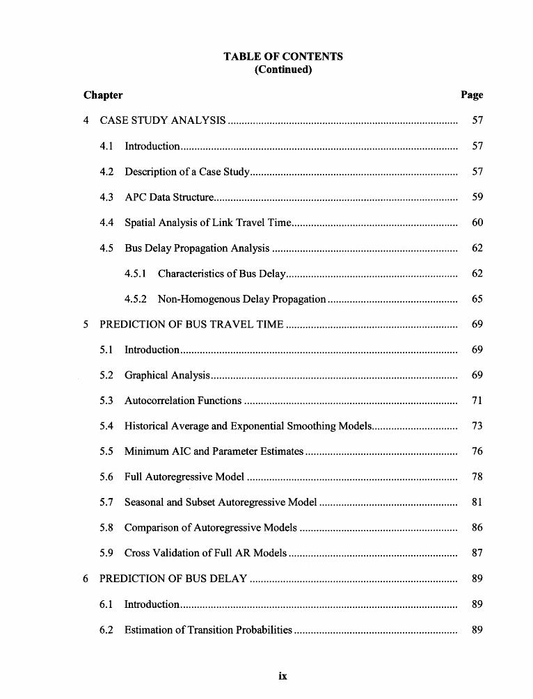
TABLE OF CONTENTS(Continued)
Chapter Page
4 CASE STUDY ANALYSIS 57
4.1 Introduction 57
4.2 Description of a Case Study 57
4.3 APC Data Structure 59
4.4 Spatial Analysis of Link Travel Time 60
4.5 Bus Delay Propagation Analysis 62
4.5.1 Characteristics of Bus Delay 62
4.5.2 Non-Homogenous Delay Propagation 65
5 PREDICTION OF BUS TRAVEL TIME 69
5.1 Introduction 69
5.2 Graphical Analysis 69
5.3 Autocorrelation Functions 71
5.4 Historical Average and Exponential Smoothing Models 73
5.5 Minimum AIC and Parameter Estimates 76
5.6 Full Autoregressive Model 78
5.7 Seasonal and Subset Autoregressive Model 81
5.8 Comparison of Autoregressive Models 86
5.9 Cross Validation of Full AR Models 87
6 PREDICTION OF BUS DELAY 89
6.1 Introduction 89
6.2 Estimation of Transition Probabilities 89
ix

TABLE OF CONTENTS(Continued)
Chapter Page
6.3 Prediction of Transition Probabilities 93
6.4 Comparison of Transition Probabilities 96
6.5 Performance Evaluation of Markov Model 101
7 BUS ARRIVAL TIME COMPUTATIONS 103
7.1 Introduction 103
7.2 Prediction of Bus Arrival Time Using Delay Propagation 103
7.3 Bus Travel Time Prediction Using Autoregressive Models 106
7.4 Combined Model of Autoregressive and Delay Propagation Models 109
8 CONCLUSION 114
8.1 Results and Findings 114
8.2 Research Contributions 117
8.3 Recommendations for Future Research 118
APPENDIX A OBSERVED TRANSITION PROBABILITIES 120
APPENDIX B PREDICTED TRANSITION PROBABILITIES 122
APPENDIX C GRAPHICAL COMPARISONS OF TRANSITIONPROBABILITIES 124
APPENDIX D CHI-SQUARE COMPARISONS 129
APPENDIX E PROBABILITY STRUCTURES OF OBSERVEDAND PREDICTED DELAY 132
REFERENCES 136

LIST OF TABLES
Table Page
3.1 Identification of AR, MA and ARMA Models Based on ACF and PACFPlot 37
4.1 Sample AVL/APC Data of a Single Bus Trip 60
4.2 Classification of Time of Day 60
4.3 Coefficient of Variation of Observed Travel Times 62
4.4 Linear Regression Slopes Between TP=10 and Downstream Time-points 66
5.1 MAPE for Historical Average and Single Exponential Smoothingof Observed Bus Travel Time 74
5.2 MAPE for Full AR Model of Observed Bus Travel Time 78
5.3 Parameter Estimates of Full AR Model for Link 10-50 79
5.4 MAPE for Seasonal AR Model of Observed Bus Travel Time 81
5.5 MAPE for Subset AR Model of Observed Bus Travel Time 83
5.6 Parameter Estimates of Subset AR Model at Lags 2 and 5for Link 10-50 84
5.7 Cross Validation of Full AR Models 88
6.1 Observed Transition Probabilities Between TP=10 and DownstreamTime-points Based on Maximum Likelihood Estimation 91
6.2 Observed Transition Probabilities Between Time-points Based onMaximum Likelihood Estimation 92
6.3 Predicted Transition Probabilities Between TP=10 and DownstreamTime-points 95
6.4 Comparison of Predicted and Observed Transition Probabilities 102
7.1 MARE of Bus Arrival Time at Time-points Using Markov Model Only 104
7.2 Final Full AR Models of Bus Travel Time 107
xi
LIST OF TABLES(Continued)
Table Page
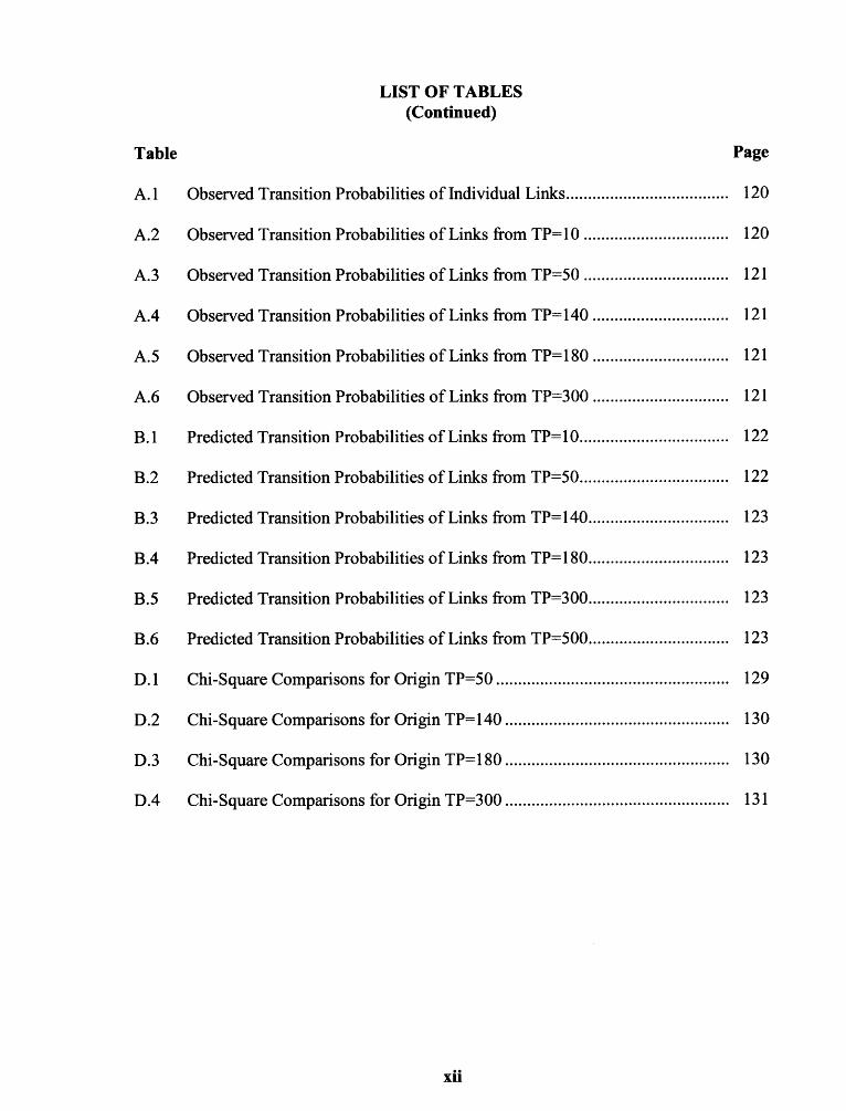
A.1 Observed Transition Probabilities of Individual Links 120
A.2 Observed Transition Probabilities of Links from TP=10 120
A.3 Observed Transition Probabilities of Links from TP=50 121
A.4 Observed Transition Probabilities of Links from TP=140 121
A.5 Observed Transition Probabilities of Links from TP=180 121
A.6 Observed Transition Probabilities of Links from TP=300 121
B.1 Predicted Transition Probabilities of Links from TP=10 122
B.2 Predicted Transition Probabilities of Links from TP=50 122
B.3 Predicted Transition Probabilities of Links from TP=140 123
B.4 Predicted Transition Probabilities of Links from TP=180 123
B.5 Predicted Transition Probabilities of Links from TP=300 123
B.6 Predicted Transition Probabilities of Links from TP=500 123
D.1 Chi-Square Comparisons for Origin TP=50 129
D.2 Chi-Square Comparisons for Origin TP=140 130
D.3 Chi-Square Comparisons for Origin TP=180 130
D.4 Chi-Square Comparisons for Origin TP=300 131
xii

LIST OF FIGURES
Figure Page
3.1 Discrete and finite state Markov chain with "m" delay states anddelay states as "On-time, Late and Early" 48
4.1 GIS diagram of bus route 62 with time-points 58
4.2 Percentage trips delayed at individual time-points with w=4 minutes 63
4.3 Percentage trips delayed at individual time-points with w=5 minutes 64
4.4 Linear regression slopes between TP=10 and downstream time-points 67
5.1 Time series plot of observed travel time for link 10-50 70
5.2 Time series plot of observed travel time for link 50-140 70
5.3 Autocorrelation plot of observed travel time for link 10-50. 72
5.4 Smoothing model diagram for link 10-50 75
5.5 Smoothing model diagram for link 50-140 75
5.6 Minimum AIC and MAPE for links a) 10- 50 and b) 50-140 77
5.7 Fit diagram of full AR model for link 10-50 80
5.8 Fit diagram of full AR model for link 50-140 80
5.9 Fit diagram of seasonal AR model for link 10-50 82
5.10 Fit diagram of seasonal AR model for link 50-140 82
5.11 Fit diagram of subset AR model at lags 2 and 5 for link 10-50 85
5.12 Fit diagram of subset AR model at lags 2 and 5 for link 50-140 85
6.1 Comparison of predicted and observed transition probabilities a)pil andb) ./92j assuming homogeneous delay propagation 97
6.2 Comparison of predicted and observed transition probabilities a) pi andb)pj assuming heterogeneou delay propagation 99

LIST OF FIGURES(Continued)
Figure Page
7.1 Histogram and normal curve of absolute values of (a) observed and(b) predicted delay at link 10-50 106
7.2 MARE values of predicted bus travel time at time-points using fullautoregressive model 108
7.3 MARE values at time-points using combined model 110
7.4 MARE values using full autoregressive model only 111
7.5 MARE values using full autoregressive and the combined modelfrom time-points a) 10 through 140 and b) 180 through 500 112
C.1 Comparison of predicted and observed transition probabilities a) pl yand b)p2j assuming heterogeneous propagation of delay for TP=50. 125
C.2 Comparison of predicted and observed transition probabilities a) plyand b)p.2.; assuming heterogeneous propagation of delay for TP=140 126
C.3 Comparison of predicted and observed transition probabilities a) plyand b)p2j assuming heterogeneous propagation of delay for TP=180 127
C.4 Comparison of predicted and observed transition probabilities a) pl yand b)p2i assuming heterogeneous propagation of delay for TP=300 128
E.1 Comparison of probability structures for link 10-140 132
E.2 Comparison of probability structures for link 10-180 133
E.3 Comparison of probability structures for link 10-300 133
E.4 Comparison of probability structures for link 10-500 134
E.5 Comparison of probability structures for link 10-900 134
E.6 Comparison of probability structures for link 10-1000 135
xiv

CHAPTER 1
INTRODUCTION
1.1 Introduction
In recent years, Intelligent Transportation Systems (ITS) have been extensively used in
planning, control and management of surface transportation systems. Traffic, highway
and transit management extensively use ITS based systems, and this trend is growing at
an increasing rate, gaining popularity amongst agencies funding and implementing these
systems. Public transit agencies have either successfully implemented, or are in the
process of implementing various ITS applications in public transit planning, bus
maintenance and operation, light rail and high speed commuter rail.
Public transit agencies rely on disseminating accurate and reliable information to
transit users to achieve higher service quality and attract more users. With the
development of ITS, the concept of providing users with reliable information about bus
arrival times at bus stops has emerged as Advanced Traveler Information Systems (ATIS)
and Advanced Public Transportation Systems (APTS). Transit agencies obtain
information in real-time on bus travel time, bus location, speed, passengers on board and
dwell time. With the help of this data, transit agencies can provide information to users
such as, arrival time and anticipated delays in advance. The information collected in real
time becomes historical information and assists transit agencies with planning,
management, and control of the system as well as the improvement of service.
1

2
1.2 Problem Statement
As part of a larger ATIS program, numerous research projects have been performed
towards developing algorithms to predict bus arrival times at bus stops. Due to the fact
that bus operation parameters and variables are highly stochastic, modeling bus travel and
arrival times has become one of the many challenging tasks among researchers. A
number of deterministic models based on regression analysis have been proposed to
estimate bus operational parameters including models to predict bus arrival time. Such
models, however, are oversimplified and may not be representative of real bus conditions
as such models do not account for the changes in bus travel time with changing traffic
and transit conditions.
A number of deterministic and stochastic models have been proposed by
researchers to predict bus operations on freeways. However, limited models exist to
estimate bus conditions on urban arterials and local streets. Hence, this research develops
models to predict bus arrival time along urban arterials and local streets based on
stochastic time series modeling of travel time and the inclusion of delay propagation in
the prediction of the bus arrival time. Delay propagation is the process where delay
incurred at an upstream bus stop is carried forward to downstream stops.
Bus arrival time prediction models based on linear and non-linear regression,
Kalman filtering and artificial neural networks do not account for the propagation of bus
delay to downstream time-points (i.e. locations long the route where the bus has to be at
predetermined times as scheduled). The existence of propagation of bus delay is not
questionable as bus drivers are constantly aware of the delay incurred in the previous
time-point and the possibility of these delays propagating to downstream time-points.

3
Hence, drivers tend to adjust their speed to reach the downstream time-points on-time and
adhere to the schedule. Some transit agencies do provide schedule adherence status to the
passengers waiting at the bus stops. However, limited research has been performed to
model bus delay and its propagation to downstream bus stops, including the possibility of
including bus delay information in the prediction of bus travel and arrival time.
1.3 Research Objectives
The primary objective of the research is to develop models to predict the bus arrival time
at stops using historical bus travel time information. The research uses a stochastic
approach to predict bus travel time and delay propagation based on historical information
of bus travel time and delay. Before any prediction models are proposed, existing bus
travel and arrival time prediction models were studied to determine their limitations. In
addition, the research established the potential for using the stochastic behavior of bus
travel time and the propagation of delay at bus stops in the prediction of the bus arrival
time.
The research focused on stochastic time dependent prediction models assuming
that bus travel times can be treated as random variables and distributed over time. In this
research, the appropriate stochastic time series models were identified. The ability of the
models to capture the temporal variations of bus travel time was also determined. Since
existing stochastic time series models do not consider the propagation of bus delays to
downstream stops, this research is also focused on modeling the propagation of delay of
buses to downstream stops. In general, the objectives of the research are outlined as
follows:

4
Develop bus arrival time prediction models based on stochastic time seriesprocesses and bus delay propagation.
Compare the performance of a number of bus travel time and delay propagationmodels based on various measures of effectiveness and evaluate the performanceof the models.
- Analyze the suitability and transferability of the proposed bus arrival time modelsto different locations.
1.4 Organization of the Dissertation
The dissertation has been organized into eight chapters. Chapter 1 consists of a brief
introduction on bus arrival prediction and its importance in ATIS. This is followed by a
discussion of the specific problem and objectives of this research. A comprehensive
literature review is presented in Chapter 2, covering past research pertaining to the
prediction of bus arrival time using various methods. In Chapter 3, algorithms to predict
bus arrival times are proposed, including a discussion of the necessary assumptions and
constraints of the proposed model. The chapter also includes a discussion on the
theoretical background of a number of time series models and stochastic Markov
processes. Chapter 4 presents a case study for which bus travel time analysis and delay
propagation were performed. Chapter 5 consists of results from the proposed bus travel
time prediction mode using autoregressive models. Chapter 6 consists of an analysis of
the bus delay prediction models using a Markov process. Bus arrival time predictions are
made in Chapter 7 using both time series methods and delay propagation methods.
Finally, conclusions about the performance of the time series models and delay
propagation models are drawn in Chapter 8. The contributions of the research are
outlined and recommendations for future research are made.

CHAPTER 2
LITERATURE REVIEW
2.1 Introduction
This literature review focused on a number of studies performed by researchers to predict
bus travel and arrival time. Through the literature review, the importance of models for
the prediction of bus arrival times for operational, management and control of bus transit
is well established. Although, the usage of bus arrival time prediction models in ATIS is
well studied, few studies have been performed on bus arrival prediction models using
stochastic time series and models that incorporate delay propagation in the estimate of
bus arrival times. In this literature review, the models and proceedings required for a bus
arrival prediction model, as proposed by various researchers, are discussed. Hence, the
literature review led to the motivation for a stochastic time series and delay propagation
model for bus arrival prediction.
2.2 Application of Bus Arrival Prediction Models
The importance of bus arrival time prediction models as a component of ATIS has been
well argued by numerous researchers (Park et al., 1995; Dailey et al., 2002; Abdelfattah
and Khan, 1998). In addition to ATIS, the Route Guidance System (RGS) and Advanced
Traveler Management System (ATMS) have also relied on accurate short-term prediction
of bus arrival times. Hence, bus arrival prediction has become a critical component of
these systems (Chien and Kuchipudi, 2002).
5
6
The purpose of both APTS and ATIS systems should be to benefit travelers on
freeways, as well as, bus passengers on urban roads by reducing their travel time and
waiting time at bus stops. The primary objective of APTS, relating to transit passenger, is
to improve the distribution of information about the public transit system such as, travel
time, delay, vehicle position (Dailey et al., 2000). Hence, the prediction of bus arrival
time at bus stops is found to be valuable information for passengers to help reduce their
waiting time.
The importance of bus arrival time prediction is more significant for trips if the
expected arrival time is relatively far into the future and the headway of the bus service
along the bus route is very long. In such cases, bus passengers are more eager to know
the bus arrival time than if the bus service is very frequent. Also, in transit operations, the
stochastic variation of bus arrival times due to other roadway conditions and vehicle
ridership could be significant. This variation can deteriorate the headway adherence of
the bus and lengthen the passenger waiting time at bus stops. Hence, providing accurate
information on bus arrival at stops includes accounting for this variation and ultimately
becomes critical for providing quality service to passengers and improving the
attractiveness of bus transit (Ding and Chien, 2002).
2.3 Data Source and Errors
Automatic Passenger Counting (APC) systems can provide real time information about
passenger and bus location (Eisele, 1997). This real time information becomes a source
of historical information for future use. Many transit agencies have incorporated an on-
board APC system into a smart bus concept. APC systems have become attractive among

7
bus transit planners and managers for bus transit management and control because of the
large amount of information provided by the APC system. As of 2000, 88 transit agencies
in the United States had operational AVL and APC systems and 142 were planning to
install them. With growing interest in using AVL systems for bus arrival information
prediction, a number of researchers have focused on using the AVL/APC system for the
prediction of bus arrival time. However, most of these bus arrivals time prediction
models used by transit agencies are proprietary and literature on the topic is not available
(TCRP, 2003).
The amount of data obtained from APC/AVL systems can be quite large in terms
of the number of records. In addition, such data often contain errors, which are generally
outliers. Chien and Kuchipudi (2002) stated that using real time data, which have a higher
standard deviation (outliers) of travel time data, can adversely affect the accuracy of the
prediction model. Hence, numerous techniques have been developed by researchers to
eliminate outliers and erroneous data (Dailey and Cathey, 2002; Dion and Rakha, 2003;
Shalaby and Farhan, 2003). However, a higher standard deviation of observed travel time
data may be inherent to the data due to the nature of traffic and transit characteristics. It is
also possible that higher standard deviations of bus travel time are due to non-recurring
events. Hence, it is apparent that before developing suitable prediction models, a
statistical analysis of trip samples should be performed to determine the standard
deviation of the bus travel time and outliers should be identified.
8
2.4 Bus Arrival Time Prediction Models
The application of bus travel and arrival time prediction models has emerged as a critical
component for many ITS and ATMS systems. Due to the inherent stochastic nature of
bus travel time, prediction and estimation of arrival time has been a challenging task. At
the same time, there is also increasing demand to predict arrival time in real time for use
in adaptive control strategies.
Private vendors have developed a number of proprietary models to predict bus
arrival times. These models have been used by a number of public transit agencies to
implement advanced public transportation information systems. Most of these algorithms
and even entire information systems are patented and are not available to the general
public (TCRP, 2003).
2.4.1 Time-Distance Model
Lin and Zeng (1999) developed multiple algorithms to predict the arrival time of buses.
These algorithms used the current location and the arrival and departure times of the bus
provided by AVL equipped buses. Using time-distance diagrams, the trajectory of the bus
is constructed using the bus position obtained from the on-board Global Positioning
System (GPS). The model consists of four different types of algorithms. Algorithm 1
used the bus location data and the pre-defined travel time matrix to determine the arrival
time at the next bus stop. The arrival time at the next bus stop is determined as the
recorded arrival time of the bus at the previous stop plus the travel time from the pre-
defined matrix. Algorithm 2 used bus schedule data in addition to bus location data. Both
algorithms assumed that the bus travels at a constant speed regardless of delay. Algorithm
3 used the bus location, bus schedule and bus delay data, to predict bus arrival time based

9
on an assumption that drivers adjust their travel speed depending on delay. Algorithm 4
was identical to Algorithm 3 but differentiated between links containing at least one time-
point and links containing no time-points. The distinction was made to introduce the
dwell time into the prediction algorithm, since the dwell times at the time-points were
found to be very high along the bus route used in the case study. The overall precision
measures of the algorithms were determined by using the average deviation of the
predicted arrival from the actual arrival time. The results showed that Algorithm 4 has the
best performance. The results obtained a minimum average deviation of predicted arrival
time from observed arrival time of 2.0 minutes and a maximum of 3.6 minutes.
Translink (Texas Transportation Institute, 2000) used a time-based algorithm to
predict bus travel times along a fixed bus route in the Texas A&M University campus.
The time-based algorithm was based on a fixed value of the travel time on the route,
determined as a simple average travel time and an average dwell time at individual bus
stops. The entire bus route was divided into one-minute zones, with the total number of
zones equal to the average bus travel time. The length of each zone is the estimated
average distance traveled by a bus in one minute. The algorithm works by geographically
locating the bus in the zone by an AVL system. The travel time to a bus stop was then
estimated by determining the number of one-minute zones the bus has to travel in order
to reach that bus stop. At bus stops that had an average dwell time value of more than one
minute, time zones would overlap and the value of the predicted travel time was then
decreased by one minute after the bus dwelled in the same time zone for more than one
minute.

10
The assumption used in the algorithm is that the simple average travel time of the
bus is sufficient to account for any variation in the bus speed due to change in roadway
conditions by time of day and pedestrian movements along the bus route. The major
limitation of the algorithm is that the bus is operated inside the campus with very limited
traffic impedance. Hence, variation in travel time is not a significant factor in the
algorithm.
2.4.2 Regression Models
The prediction of bus travel and arrival time on urban corridors is a difficult task because
of the stochastic nature of transit operations and the impact of factors such as passenger
demand at stops, traffic control and interaction with other vehicles. The estimation of bus
travel time can be obtained using classical statistical analysis such as regression models.
Frechette and Khan (1997) used Bayesian regression analysis to estimate
vehicular travel times between links in CBD locations. Data for the independent variables
were obtained using a video camera. The independent variables included volume of
through, left and right turning vehicles, number of signalized intersections, percentage of
stopped vehicles on each link, and the percentage of heavy vehicles. Though these
parameters can be obtained using a video camera, this method has two major limitations.
Firstly, installation of a video camera would be required in each and every intersection
along the bus route, which would be expensive. Also, data extraction from the video
camera would be a difficult process and not a real time process compared to AVL
technology. The regression models were developed for both one-way and two-way street
configurations. Although the results were quite appreciable in terms of their high R 2
values, the implementation of the algorithm to predict bus travel times requires collection

11
of a large number of independent variables. The authors recommended that developed
models could be incorporated into an ATIS to provide average vehicular travel times.
Abdelfattah and Khan (1998) developed non-linear regression models of bus
delays. The independent variables that influence bus delays in mixed traffic lanes were
collected using a video camera. This field information was used as input into the micro-
simulation package NETSIM and various measures of effectiveness were obtained. The
regression models used a number of independent variables such as link length, number of
bus stops per link, number of buses per link, vehicle turning movements, traffic density
of heavy vehicles, density of traffic signals and number of passengers riding the bus.
These variables are not easily available for the prediction of bus travel time, considering
the amount of data and method of data collection required. The R 2 obtained from the
regression models were above 0.8. Bus arrival times were determined from average bus
speed plus expected delays estimated by the developed regression models. A constant bus
speed was used to determine the bus travel time without any delays. The average
difference between the estimated and actual bus arrival times of 70 buses over a 30-
minute period was determined. For two streets under study, the average difference was
found to be less than 30 seconds.
Patnaik et al. (2004) developed a multivariate linear regression model to estimate
bus arrival time between time-points along a bus route. The data were obtained from the
APC system installed on buses. The travel time of the bus between time-points was
estimated using linear regression of the historical travel times between the time-points.
The linear regression model consisted of independent binary variables to represent time
of day of the bus trip, dwell time, number of stops and distance between time-points. The

12
study used cumulative values of dwell time and number of stops between time-points as
independent variables, since individual values of dwell time at stops would not be
significant compared to the total travel time between time-points. The models showed
significant results in terms of higher R 2 values, but did not present comparisons between
observed and predicted bus arrival times.
2.4.3 Artificial Neural Network Models
Artificial neural networks (ANN) and in particular multilayer neural networks that utilize
a back propagation algorithm have been used to predict link travel time for buses as well
as for other vehicles. The majority of the neural network applications used in the field of
transportation are conventional ANN models.
Ding and Chien (2002) developed link-based and stop-based artificial neural
networks (ANN) for predicting bus arrival times in real time. The link-based ANN is
designed to predict bus arrival times by accumulating bus travel times on all traversed
links between pairs of stops. Unlike the link-based ANN, the stop-based ANN estimates
the bus arrival time to a downstream stop using traffic conditions instead of bus travel
times accumulated on all traversed links. For training the ANN models, back propagation
learning algorithms were used.
The factors affecting bus arrival time (e.g., volumes, average speed, delays) were
inputs for link-based and stop-based ANN models. The bus arrival times predicted by
ANN models were compared with results from the micro-simulation model CORSIM,
which was calibrated with field data. The Root Mean Square Error (RMSE) between
simulated bus arrival and predicted arrival time increased as the number of downstream

13
stops increased. The RMSE values increased from 1 minute to 4 minutes showing that the
model performed well for the study bus route (Ding and Chien, 2002).
2.4.4 Kalman Filter Models
Kalman filters have also been used for prediction of bus travel time as well as vehicle
travel times on freeways for incident detection models. Bae and Kachroo (1995)
developed a Kalman filter model to estimate arterial travel time for buses by using AVL
equipped buses as probe vehicles. A prototype bus arrival time estimation model was
developed based on an online parameter adaptation algorithm. Based on the dynamics of
both single and multiple stops, a prediction model for bus arrival time was developed.
The model relied on an extended autoregressive model and considered time varying
passenger boarding and alighting rates.
Chien and Kuchipudi (2002) developed a model to predict travel time using real-
time and historical data based on Kalman filters. In the research, a Kalman filtering
algorithm was used to update the state variable (travel time) continuously as new
observations became available. In addition to the real time information, the research
considered the use of aggregate data from previous time intervals and days as historical
seeds to evaluate the prediction accuracy.
Dailey et al. (2000) used time series data obtained from an AVL system to predict
bus arrival time. The data consisted of time and location pairs and was used with
historical data in an optimal filtering framework to predict bus arrival times. The filtering
model continuously predicts the arrival time of the bus as a function of both time and
space. The filtering model assumed that vehicle locations are available irregularly,
typically on a one to five minute basis. The vehicles are assumed to move with constant
14
speed over a limited distance. The variability of the modeling process is normally
distributed and includes the starting and stopping motions of the vehicles. The algorithm
provided predicted bus arrival times up to an hour in advance. Using Kalman filters as an
optimal filtering technique, the bus arrival time was determined. The model, however, did
not explicitly use the variability of the bus travel time during different times of day to
include temporal variability of bus travel time and assumed that such variability is
included in the modeling process. The model is entirely based on the trajectory motion of
the bus, which relies on a high polling frequency, so that the bus position is updated
within minutes.
Shalaby and Farhan (2003) proposed two Kalman filter algorithms for the
prediction of bus running time and passenger dwell time alternately in an integrated
framework. The "Link Running Time Prediction Algorithm" made use of the last three
days of historical data of the bus link running time for the prediction. The bus link
running time for the previous bus on the current day at the current time is also used to
predict the bus running time one period ahead. The "Passenger Arrival Rate Prediction
Algorithm" employed similar historical data on passenger arrival rates to predict the
dwell time. The predicted arrival rate is multiplied by the predicted headway and by the
passenger boarding time. The bus arrival time prediction results obtained from the
Kalman filter model were compared with the results obtained from historical average,
regression and artificial neural network models. The Kalman filter model produced a
Mean Relative Error (MRE) between 0.044 and 0.087, while predicting travel time using
four previous days of data and comparing these data with the data observed on the fifth
day. The results showed that the Kalman filter model performed similar to regression and

15
ANN models in the normal condition scenario without any congestion. However, the
Kalman filter model outperformed other models in special event and lane closure
scenarios. The performance of algorithms was tested using data from microscopic
simulation.
2.5 Bus Delay Propagation
2.5.1 Delay Propagation Models
Few bus arrival time prediction models have included the propagation of bus delay at
downstream stops, though the importance of delay propagation has been stated in
previous studies (Dailey et al., 2000). For the prediction of bus arrival times, it is
important to incorporate into prediction algorithm information on bus delays, specifically,
how these delays propagate as a bus travels over a route. In this context, bus delay is
defined as the deviation of bus arrival time from the scheduled arrival time. Very often,
bus stops are not equidistant and links connecting the stops are not homogeneous in
traffic characteristics. The correlation of delay between any two stops is hence different,
requiring an approach to determine bus delays by link. However, the degree of
correlation is related to the amount of built-in slack time embedded in the bus schedule
(Lin and Bertini, 2002). The prediction of bus arrival times at subsequent bus stops
requires that the delay incurred at an upstream stop should be considered to propagate to
downstream stops. Hence, considerations of bus delay propagation to downstream stops
due to delay at upstream bus stops have to be made while predicting bus arrival times at
the downstream bus stops.
16
Many bus transit systems provide real-time schedule adherence status to their
operators on an in-vehicle display terminal (Strathman et al., 2001). Using the schedule
adherence status, skilled bus operators constantly adjust their speed to keep their buses on
schedule and try to avoid being too late or early. When a bus is delayed at a current bus
stop, the bus operator's ability to reach the downstream stop in time depends on the
amount of slack time built into the bus schedule and the characteristics of traffic along
the link.
Limited studies have been performed regarding the application of delay
propagation in modeling bus arrival times. Bus delay propagation in the form of simple
linear relationships with travel distance has been used (Lin and Zeng, 1999). The model
used a dimensionless input factor A E {OM d.
in the prediction model, where 2= 11 ,
is the distance between stops i and j and d is the total length of the trip.
Lin and Bertini (2002) formulated a Markov chain model to capture the
propagation of bus delay at downstream bus stops. It was assumed that the bus stops were
uniformly spaced with equal distance (homogenous condition) and data used to
demonstrate the delay propagation model were not a real-world data.
The research described in this dissertation proposes the use of Markov chains to
model the propagation of bus delay to downstream stops. Previous studies have
demonstrated the use of finite state Markov chain models to simulate and predict traffic
conditions on freeways and arterials. These models were used in conjunction with
microscopic simulation to describe driver behavior in situations such as, traffic
assignment and estimation of vehicle delay between signalized intersections (Evans et al.,
2001; Lin et al., 2003).

17
Lin et al. (2003) developed a simple approach to predict delay of vehicles along
an arterial based on Markov chains. The approach used a one-step transition matrix that
related the delay of through vehicles at an intersection to the delay status at the adjacent
upstream intersection. The parameters of the transition matrix were determined based on
three key factors including, flow conditions at the intersection, the proportion of net
inflows into the arterial from the cross streets, and the signal coordination level. The
research also assumed homogeneous conditions between adjacent intersections.
Numerical results show that the model can yield delay predictions with a reasonable
degree of accuracy under various traffic conditions and signal coordination levels. The
model was not validated using field data and the results from the model were compared
with the simulated results. The models were not used to predict bus arrival times.
2.5.2 Finite State Markov Chains
Numerous studies are available regarding estimation using Markov chains (Anderson and
Goodman, 1957; Meshkani and Billard, 1992, Robertson, 1990). The simplest method to
estimate transition probabilities is to determine the ratio of individual transitions
observed to the total number of transitions. Numerous studies have been performed to
improve the determination of transition probabilities. Anderson and Goodman (1957)
developed a maximum likelihood method to determine transition probabilities of a finite
Markov chain for large sample data. Anderson and Goodman (1957) and Lee et al. (1968)
compared the maximum likelihood method and Bayesian estimators to estimate a
transition probability matrix when aggregate proportion data were used. Bayesian
estimators improved the overall estimation of the process over least square and maximum
likelihood methods. The Empirical Bayes method is able to produce non-zero transition

18
probabilities, which is common while using a maximum likelihood estimation method for
smaller sample size. However, empirical Bayes methods require more than one data set
that is independent and identically distributed, which may not be always available.
2.6 Stochastic Time Series Models
2.6.1 Stochastic Models for Traffic Prediction
Time series prediction methods have been established as a prominent statistical method
for long term prediction of social and economical variables in planning and management
areas. Due to recent developments in ITS, the same statistical prediction methods used
for social and economic variables have been used in the prediction of traffic parameters.
However, predicting traffic variables are mostly limited to short term prediction, in terms
of minutes or hours rather than days or months, which is more common in long term
prediction of economic variables. Hence, researchers are more focused on developing
time series methods for use in short term traffic prediction.
A number of travel time prediction models have been developed for freeway
conditions mainly for the purpose of incident detection. These prediction models rely on
data obtained from detectors placed at strategic locations along freeway segments.
Distinctions between travel time prediction models in freeway conditions and urban
arterial or downtown conditions are mainly related to statistical uncertainties in
prediction. Due to the fact that fluctuations of traffic conditions exist on arterials and
freeways, travel time is considered time dependent and stochastic. Compared to urban
roadways where a stochastic process is prominent, it is more common among researchers
to consider travel time to be deterministic on freeways. Compared to freeways, a limited

19
number of stochastic time dependent models have been proposed to predict bus travel and
arrival time along urban arterials (Hamed et al., 1995; Park et al., 1995).
Short term prediction of traffic variables can be distinguished as either empirical
or based on traffic flow theory. Empirical methods are based on fairly standard statistical
methodology of linear and non-linear regression and adaptive filtering methods. In traffic
process theory, fairly complicated origin-destination flows, traffic assignment and
distribution along paths and links are used for traffic prediction (Arem et al., 1997). Due
to the simplicity of empirical methods in comparison to methods based on traffic
processes, a number of researchers have used time series prediction methods to predict
traffic parameters (Lee and Fambro, 1999; William et al., 1998; Ross, 1982; Ahmed and
Cook, 1979).
Lee and Fambro (1999) developed a Subset Autoregressive Integrated Moving
Average Model (S-ARIMA) for short-term prediction of freeway traffic volume at two
sites in San Antonio using data obtained from the TransGuide project. The study
concluded that time series models are effective for short-term prediction of vehicle travel
time along a freeway. Williams et al. (1998) used seasonal ARIMA models to predict
urban freeway traffic flow assuming that time series of traffic flow data has
characteristics of being periodically cyclic. The 15-min flow rate was obtained from loop
detector data from locations at Capital Beltway in northern Virginia. The missing data
were replaced by using a Kalman filter method and simple average of historical
observations.
Ross (1982) analyzed 5-minute volumes obtained from 24h/day count from loop
detectors along a freeway and an urban arterial. Different smoothing constant (a) values

20
for exponential smoothing models were compared at different days for urban arterial time
series data to obtain an optimal value of a. The optimal value of a was obtained by
differentiating the mean square error function of the model for different values of a. The
study also suggested the use of varying a values for different times of the day instead of
using the fixed value of a for the entire week.
Ahmed and Cook (1979) used a Box-Jenkins approach to determine ARIMA
models for predicting traffic volume and occupancy. The data used to develop the models
were obtained from detectors along freeway sections and aggregated to 30 and 60
seconds for the duration of one peak period. The ARIMA models were compared with a
moving average model and double exponential smoothing models using the mean
absolute error and mean square error. The ARIMA models outperformed the moving
average and double exponential smoothing models
Smith et al. (2002) developed seasonal ARIMA models to predict traffic flow
along London Orbital Motorway using 15-min traffic flow obtained from detectors on the
freeway. Instead of using a visual inspection method to determine the parameters of the
ARIMA model, which is the foundation of the Box-Jenkins approach, the research used
Akaike Information Criterion (AIC) to search for a suitable ARIMA model. Box-Jenkin's
method is often termed as subjective because of the subjective method of choosing the
model order using visual interpretations. By using the appropriate AIC, the subjectivity of
selecting the appropriate model can be removed.

21
2.6.2 Comparison of ARIMA Models
It is certain from the literature review that one category of time series models cannot
guarantee that it will always give higher prediction accuracy than another category of
time series model. Hence, researchers often use a number of time series models and
compare the performance measure of the model to determine the best model. Lee and
Fambro (1999) developed a full ARIMA model (F-ARIMA), an exponential smoothing
model and a subset ARIMA model for comparison purposes. Exponential smoothing
models gave slightly better result than other time series models, except for subset
ARIMA model which gave the best results. The researchers concluded that exponential
smoothing models should be considered for short-term prediction because these models
were also determined to be easier to implement than ARIMA models.
Williams et al. (1998) also compared predicted freeway traffic flow developed
using seasonal time series, seasonal exponential smoothing, neural network and historical
average models. The seasonal ARIMA model produced the smallest Mean Absolute
Error (MAE) and Mean Absolute Percentage Error (MAPE), followed by the seasonal
exponential smoothing model then the neural network model and finally the historical
average model. Ahmed and Cook (1979) also found better results from ARIMA model
compared to exponential smoothing and historical average models.
Exponential smoothing and historical average models are non-parametric methods
of time series trend estimation and not entirely used for prediction purposes. However,
these models are still used for prediction purposes due to their simplicity in computation.
Hence, these models are popular for one-step-ahead univariate real time prediction
(Makridakis and Wheelwright, 1978).

22
AR, MA and ARIMA models are not adaptive such as, Kalman filtering and are
not widely used for real time prediction. However, modified forms of AR, MA and
ARMA models are available to work as an adaptive model although implementation of
such models is computationally intensive (Brockwell and Davis, 2002; Chatfield, 2000).
2.7 Summary
The literature review revealed that bus arrival time prediction models take into account
historical vehicle operations including the bus arrival time for the last several buses on
the same route over the previous several months, and traffic patterns. These prediction
algorithms use historical data as a basis to state the existing traffic conditions at the time
of prediction. The historical profile of travel times is the best knowledge of the past for
use as a basis for the prediction of travel times in the future (Franco and Taranto, 1995).
Time-Distance models (Lin and Zheng, 1999) were developed for rural settings,
where traffic congestion is not a major issue. Hence, these algorithms may not be
applicable to urban areas where congestion is a major issue. These algorithms are also not
able to explain fluctuations in arrival time of the bus due to changes in traffic volume and
other traffic parameters. The model assumed that the delay at a downstream stop is
directly proportion to the travel distance between the bus stops and is propagated to
downstream stops in the same magnitude if the distances between the links are equal.
This assumption may be reasonable in a rural environment where traffic characteristics
between the bus stops may not have a major influence on frequency and amount of bus
delays. However, in an urban environment, equidistant links may have plenty of
variations in traffic characteristics, which in turn could affect bus delays.

23
The regression models were developed to determine the vehicular travel time and
bus delays. Even though the obtained R2 values were statistically significant, the studies
did not include the prediction of bus arrival times (Frechette and Khan, 1997; Abdelfattah
and Khan, 1998). The models took into account independent factors that affect the travel
time of the bus along a link such as, distance, speed, number of intersections, and traffic
volume. The models do not take into account the presence of temporal variations of bus
travel times and propagation of delays to downstream stops. In addition, due to the large
number of data required to develop regression models, both studies used output from a
micro-simulation package. The field data were collected as an input to the micro-
simulation package.
The current geographic location of the bus was used to predict the future location
of the bus and predict bus arrival times using Kalman filtering. The model relies on high
frequency of availability of the GPS location, which is most difficult in dense cities with
high rise structures (Dailey et. al, 2000). Another bus arrival time prediction model using
Kalman filter model was based on historical bus travel time information and constant
headway of the bus (Shalaby and Farhan, 2003). Contrary to Kalman filter and regression
models, ANN model requires more intensive computation and data requirements.
The literature review provided a background on limited number of models to
predict bus arrival times based on assumptions of stochastic variation of bus travel times
and delay propagation. Also, literature about proprietary prediction models developed by
private vendors is not available, which are actually being implemented by the transit
agencies. The models described in the literature review are either deterministic models
such as time-distance or regression models or too complicated such artificial neural

24
network models. Except time-distance model, all the other models require a large number
of independent variables. Many of these variables are not available to the transit agencies.
In comparison to numerous studies in bus travel time prediction, the literature
review revealed that the application of delay propagation to predict bus arrival times has
been limited. It is important to incorporate information on bus delay into the bus arrival
time prediction algorithm.

CHAPTER 3
ALGORITHM AND METHODOLOGY
3.1 Introduction
This chapter describes the assumptions used for the identification and implementation of
time series and Markov chains to predict bus arrival times. The algorithms to obtain the
bus arrival time prediction is presented, which is followed by a theoretical background of
the stochastic process of time series models and Markov chains, which forms a basis to
obtain the bus arrival prediction models.
3.2 Assumptions and Constraints
Conceptually, time series models rely on data from historical time periods for the
prediction of future time periods. The time series models presume that a pattern or
combination of patterns occurs periodically over time and these patterns can be defined
using mathematical functions. As a consequence, one can also assume that historical data
can be used to identify the patterns or combination of patterns of bus travel time. The
motivation for using time series models for predicting bus travel times is that it is not
necessary to establish relationships between independent variables and the dependent
variable under study in a time series model as it is needed in regression models.
Time series prediction models determine what would happen in successive time
periods rather than why it would happen. Hence, the bus arrival prediction model is not
necessarily concerned with why the bus arrived at a specific future time period, but is
more concerned with when the bus would arrive. Unlike regression and artificial neural
25

26
network models used for predicting bus travel times, time series models do not attempt to
discover the factors affecting bus travel times.
Time series models assume that the variable under study is the function of past
values in time and these past values are available in discrete and equispaced time
intervals. The function can be characterized by some reoccurring pattern or combination
of patterns. The following relationship demonstrates these assumptions:
zt = f(zt-hzt-2, ,zt_p) (3.1)
Where,
zt = Predicted value at future time t
zt -1 , zt-2, = Historical values at equally spaced times t-1, t-2,...
p= Number of time periods used in the forecast
In Equation 3.1, the predicted value of the variable is determined by a function of
historical values of the same variable. Unlike regression models, the explicit relationship
between the historical values and the predicted value is not significant.
In this research, the prediction of bus travel time assumes that some recurring
pattern of bus travel time exists during different times of the day due to recurring traffic
conditions. Based on these patterns, future bus travel times can be predicted. The
foundation of model building for discrete observations over time using time series
methods is the assumption of a stochastic process, where the prediction model describes
the probability structure of the sequence of observations. The future value is predicted by
determining the probability distribution of the population using sample past values.
Most stochastic bus arrival time prediction models lack factors that account for
bus delay propagation to downstream stops. Hence, a separate analysis of bus delay
27
propagation is provided in this dissertation assuming that bus delay can be observed as a
stochastic Markov process. The individual bus trips are assumed to be independent and
identically distributed, which is a necessary condition to implement Markov chains. The
predicted bus arrival time is presented in the dissertation using delay propagation only
and also using a combination of both stochastic models to predict travel time and bus
delay propagation to downstream stops. The bus arrival prediction model using only bus
delay propagation requires existing bus schedule information. Bus schedule information
is assumed to be the best estimation of future bus arrivals in the absence of any delay at
an upstream stop or at the origin.
3.3 Bus Arrival Time Prediction Algorithms
3.3.1 Delay Propagation Model
The prediction of the bus arrival time using delay propagation at downstream stops is
based on predicted delay and the scheduled arrival time at each time-point. It is assumed
that the prediction of the bus arrival time is solely based on the prediction of the bus
delay at downstream stops due to observed delay at the origin stop. The predicted arrival
time of the bus at the downstream stop is determined by modifying the scheduled arrival
time of the bus by the predicted delay of the bus. The algorithm to predict the bus arrival
time using the predicted delay and scheduled arrival time is presented as follows:
At t < (A i ),
(Ai) = (D0,1) + (SAT 1 ) (3.2)
(A2) = (SAT 2) + (D0,2) (3.3)
••••

28
(Ad) = (SATa) + (Do,d) (3.4)
Where,
(Do,i) , (Do,d) = Predicted delay at time t at the origin (i=0)
(A 1 ), , (Ad) = Predicted arrival time of bus at time-point 1 to destination d
(SAT 1 ), (SATd) = Scheduled arrival time at time-points/ to destination d
At any time "t", when the bus has left the origin time-point and has not reached
the next time-point, the arrival time of the bus at the subsequent downstream time-points
can be predicted using Equations 3.2 through 3.4. The arrival time of the bus at any
downstream time-point is predicted based on its scheduled arrival time at the time-point
and the delay predicted at the time-point. This delay is a consequence of the delay
observed at the origin time-point. In Equations 3.2, (D0,1) is determined using a transition
matrix of delay states between time-points 0 and 1. However, (D0,2) . , (D04) are
determined using the successive application of the Markov chain (Kemeny and Snell,
1976), based on the following relationship:
Do,i>o = Po.( P( 1)).sT (3.5)
Where,
D0,,,0 = Predicted delay at i, given a delay state at 0
Po = Initial probability vector at i=0
(P(1)) 1 = ith Power of transition matrix P(1), between time-points 0 and / = P(1)
sT = Transpose of delay states at i=0
The delay at time-points 1 through d can be determined by using the integer
multiple of the transition probability matrix between time-points 0 and 1, which is P(1),
as shown in Equation 3.5. The equation is used to predict delay at downstream time-

29
points based on a specific time-point and it is assumed that the time-points have similar
traffic and geometric characteristics. The power of the transition matrix in Equation 3.5 is
based on the assumption that the delay states between two time-points are homogenous
having similar traffic characteristics. However, time-points may not be similar in
character. For example, the distance between two time-points can be different. To reflect
the heterogeneity of delay states between two time-points, Equation 3.5 is changed as
follows:
Do,i>0 = Po.P(1).P( 2 ) P(i).sT (3.6)
Where,
Da i>0= Predicted delay at i, given a delay state at 0
P0 = Initial probability vector at i=0
P(1), P(2), P(i) = Transition matrix between time-points 0 and 1, 1 and 2,
and i-1 and i.
ST = Transpose of Delay States at i=0
The heterogeneity between the links is reflected by using individual probability matrices
corresponding to each consecutive link instead of using the • th power of the transition
probability matrix P(1). This is shown as Equation 3.6, which consists of individual
transition matrices.
Similarly, when the bus has left time-point 1, the origin time-point is now 1
instead of 0. The transition matrices and the delay states are changed to reflect the delay
at time-point 1 and the subsequent delay propagation at downstream time-points. Hence,
Equations 3.5 and 3.6 are changed as follows to include the observed delay at time-point
1 and predict the delay at downstream time-points (1>1).

30
D0, 1 = Pp.( P(2 pi .sT (3.7)
Where,
Di,,,/ = Predicted delay at i, given a delay state at 1
Po = Initial probability vector at i=1
P(2) = Transition matrix between time-points 1 and 2
ST = Transpose of Delay States at i=/
D0, 1 = Po .P(2).P(3) P(i).sT (3.8)
Where,
P(2), P(i) = Transition matrix between time-points 1 and 2, 2 and 3,.. i-1 and i
Hence, the algorithm to predict bus arrival times at time-point 2 through d is
updated as follows to reflect the new position of the bus:
At (Ai) < t < (A2),
(A2) = (SAT2) + (D1,2) (3.9)
(Ad) = (SATd) + (D1,d) (3.10)
Where,
(D 1 ,2) , , (D1,d) = Predicted delay at time-points 2 through d from the origin
time-point (i=/)
At time-point i=0, the delay at the downstream time-point (Do,2) is based on the
transition probabilities of delay states between i=0 and i=1. As the bus traverses
downstream when i=1, the prediction of delay at time-point i=2 (D1,2) is based on
transition probabilities of delay states between i=1 and i=2.

31
3.3.2 Travel Time and Delay Propagation Model
In this research, the arrival time of a bus at a time-point is determined by using a
predicted value of the bus travel time and the dwell time at each time-point. In addition to
travel and dwell time, a third component of the predicted delay at downstream time-
points is introduced during the prediction process. Unlike the algorithm described in
Section 3.3.1, this algorithm does not require the scheduled bus arrival time at time-
points. Instead, the algorithm requires the observed arrival time of the bus at the previous
time-point.
The bus arrival time at each time-point is determined by using a combined
prediction of the stochastic travel time and the delay propagation. The historical values of
bus travel times are used to predict the future bus travel time at individual time-points
using an autoregressive (AR) model in combination with the predicted delay. This
combined algorithm to predict bus arrival time is shown by the following equations:
At, DEP0 < t < (Ai= i )
(A1)= (DEP0) + (TTo,i) + (D o , 1 )
(A2)= (DEP0) + (170,2) ( 30,2)
(Ad) = (DEP0) + (Tro,d) (Do,d)
Where,
(DEP0) = Observed departure time at the origin (i=0)
(3.11)
(3.12)
(3.13)
(A1), (Ad) = Predicted arrival time of bus at time-point 1 to destination d
(D0,1) , (Do ,d) = Predicted delay at time-point 1 to d due to delay at the
origin (1=0)

32
(TT0 , 1 ), .... (T1'0,d) = Predicted travel time between time-points 0 to 1, ... 0 to d.
In Equation 3.11, the arrival time of the bus at the first time-point (i=/) is
determined by using the observed bus departure time at the origin (DEP0) and the
predicted travel time and delay due to observed delay at the origin time-point. The bus
arrival time at subsequent time-points (i> 1) is determined by using equations 3.12 and
3.13. Hence, when the bus is at the origin time-point (i=0), the arrival time at all the
downstream time-points can be predicted using Equations 3.11 through 3.13. The
generalized expanded forms of Equations 3.11 through 3.13, where the travel time and
delay are expressed using an autoregressive model and a Markov process, respectively
are as follows:
(Ai) = (DEP 0) + (colzt_ i +92zt_2 + 9pzt-p)0,i +(Po.P(/).ST) (3.14)
(A2) = (DEP0) + (9Tzt_1 +92zt_2 +
Or,
(A2) = (DEP0) + (91 zt -1 ± 92zt-2 +
9 p zt-d0,2 +( PO.P0,2.S T )
(3.15)
9pzt-do,2 +(Po.P(/).P(2 ).ST ) (3.16)
(AO_ (DEP0) + /I 9/Zi-/ +92Zt-2 + 9pZi-pk,d+ +(PO4,d'ST )
Or,
(Ad)--(DEP0)+ (k Corzt—/ +92zt-2 + 9pzt-p )0,d ±( PO
(3.17)
P(1).P(2) P(d).ST ) (3.17)
Equations 3.14 through 3.17 represent the expanded form of Equations 3.11
through 3.13. In these new equations, the travel time on a link is defined by the

33
autoregressive model and the delay incurred at the downstream time-point due to the
upstream time-point is defined by the Markov model. The difference between Equations
3.15 and 3.16 is that Equation 3.15 requires inclusion of a transition matrix between time-
point 0 and 2 (Po,2) and Equation 3.16 requires the inclusion of transition matrices
between time-points 0 and 1 (P(1)) and 1 and 2 (P(2)).
As the bus traverses towards the downstream time-points, the observed value of
the departure time at the previous stop is used in addition to the observed delay at the
previous stop and the arrival times of the bus at the remaining time-points are updated.
Hence, if the bus has an unexpectedly longer observed delay at a previous time-point, the
arrival time at the following time-point is predicted accurately. For time-points located
downstream of the origin (i=0) time-point, the following equations are used to predict the
arrival times:
At, (DUI) < t < (A2)
(A2)= (DEP1) + (Tvri,2) + (D1,2)
(A3)= (DEP1) + (171,3) + (D1,3)
••••
(Ad) = (DEP1) + (TT1,d) + (D1,d)
At, (DEP2) < t < (A3)
(A3) — (DEP2) + (TT2,3) + (D2,3)
(3.19)
(3.20)
(3.21)
(3.22)
(Ad) — (DEP2) + (TT2,d) + (D2,d) (3.23)
Where,
(DEP 1 ), ..., (DEP2) = Observed departure time of bus at time-point 1 and 2.

34
(A2), (Ad) = Predicted arrival time of bus at time-point 2 to destination d.
(D1,2) , , (13 1 ,d) = Predicted delay at time-point 2 through d due to delay at
time-point 1.
(D2,3) , , (D2,d) = Predicted delay at time-point 3 through d due to delay at
time-point 2.
(TT1,2), (17d_1,d) = Predicted travel time between two consecutive time-
points.
The predicted values of bus arrival time are determined by using Equations 3.19
through 3.23, for time-points other than the origin (1<i<d). In these equations, time of
prediction is after the departure time of the previous time-point and before the arrival
time of the time-point (DEPH < t < Ad. The expanded forms of Equations 3.19 through
3.21 are as follows:
(A2) = (DEP 1 ) + +92zt_2 + 9pZi_ p )1 ,2 ( Po .P( 2 ).ST ) (3.24)
(A3) = (DEP 1) (9/zt--] +92zt-2 9pzi_p)1,3 +( Po .P( 2 ).P( 3 ).ST ) (3.25)
(Ad) = (DEP 1) + (91zt-1 +92zt-2 9pzt-p )1,d + Po.P( 2 )....P( d ).S T ) (3.26)
35
3.4 Selection of Travel Time Prediction Models
3.4.1 Box-Jenkins Approach
Box and Jenkins (1970) developed a systematic procedure to analyze and forecast time
series using ARIMA models. Hence, this procedure is often called the Box-Jenkins
methodology. The Box-Jenkins methodology to identify an appropriate ARIMA model is
an iterative process and consists of four basic steps. The first step consists of identifying
autoregressive, difference and moving average orders of the model, which are
represented by p, d and q, respectively. This is done based on autocorrelation and partial
autocorrelation plots of the time series. In the estimation process, the parameters of the
model are estimated using the maximum likelihood method. Diagnostic tests are then
performed to determine the adequacy of the model. If the model is considered adequate, it
is used to forecast future values. If not, then the iterative cycle of identification,
estimation and diagnostic checking is repeated until an adequate model is found.
3.4.2 Autocorrelation and Partial Autocorrelation Functions
The autocorrelation and partial autocorrelation functions of the differenced time series
provide clues about the choice of the orders ofp and q for the autoregressive and moving
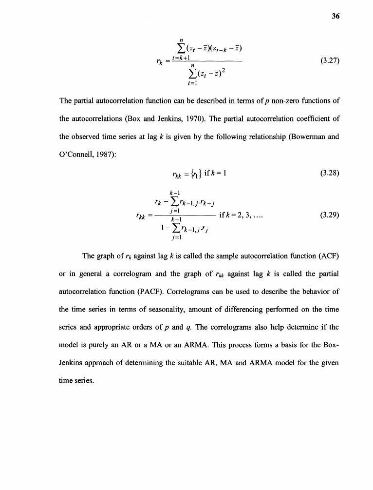
average models (Box and Jenkins, 1970). The autocorrelation function of a time series is
similar to correlation in regression models, except that the autocorrelation function
defines the relationship between values of the same variable at different time periods or
lags (k). For a time series (z1, z2, z3, ...), the sample autocorrelation at lag k is given by the
following relationship (Bowerman and O'Connell, 1987):
rkk = {II} if k = 1
k-1rk — Erk _ij .rk _i
i= 1k-1
1— Erk_i, j -rjj=1
rkk =
(3.28)
(3.29)if k = 2, 3, ....
36
n
E (zt _ 0(zt _k —±-)t=k+1 rk =
nE(zt _ 2) 2
t=1
(3.27)
The partial autocorrelation function can be described in terms of p non-zero functions of
the autocorrelations (Box and Jenkins, 1970). The partial autocorrelation coefficient of
the observed time series at lag k is given by the following relationship (Bowerman and
O'Connell, 1987):
The graph of rk against lag k is called the sample autocorrelation function (ACF)
or in general a correlogram and the graph of rkk against lag k is called the partial
autocorrelation function (PACF). Correlograms can be used to describe the behavior of
the time series in terms of seasonality, amount of differencing performed on the time
series and appropriate orders of p and q. The correlograms also help determine if the
model is purely an AR or a MA or an ARMA. This process forms a basis for the Box-
Jenkins approach of determining the suitable AR, MA and ARMA model for the given
time series.

37
Table 3.1 Identification of AR, MA and ARMA Model Based on ACF and PACF Plot(Bowerman and O'Connell, 1987)
Model AutocorrelationFunction
Autoregressive Exponential Decayprocess of order pMoving average Spikes at lag 1 to q and 0process of order q after lag q Mixed AR and MA Exponential Decayprocess
Partial AutocorrelationFunction
Spikes at lag 1 to p and0 after lag pExponential Decay
Exponential Decay
The statistical significance of rk at any lag k is determined by the t-statistic given by the
following relationship:
irk rk
(3.30)Srk
Where,
0/2( k---1
Srk 1 + 2 Er ?a+0" j=1
The statistical significance of rkk at any k is determined by the t-statistic given by the
following relationship:
trkk = rkk (3.31) 1
(n — a +1)1/2
As a rule of thumb, it can be concluded that rkk = 0 if 41 2. In addition, the ACF and
PACF plot can also indicate the seasonality in the time series by showing large positive
values of rk at the seasonal period. If the seasonal time series is not stationary, a seasonal
differencing is done to create stationary time series. The autocorrelation and partial
38
autocorrelation plots indicate the amount of seasonal differencing required by showing
significant peaks at lags corresponding to the seasonal time periods.
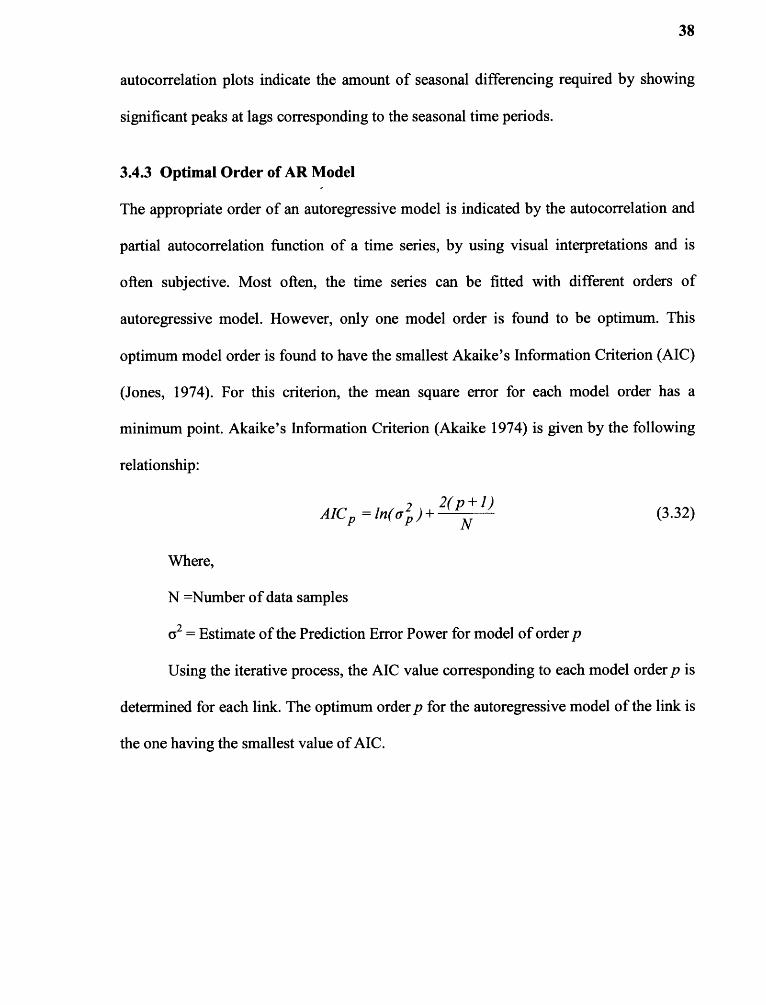
3.4.3 Optimal Order of AR Model
The appropriate order of an autoregressive model is indicated by the autocorrelation and
partial autocorrelation function of a time series, by using visual interpretations and is
often subjective. Most often, the time series can be fitted with different orders of
autoregressive model. However, only one model order is found to be optimum. This
optimum model order is found to have the smallest Akaike's Information Criterion (AIC)
(Jones, 1974). For this criterion, the mean square error for each model order has a
minimum point. Akaike's Information Criterion (Akaike 1974) is given by the following
relationship:
AICP =ln(u 2 )+ 2( P 1 ) N
Where,
N =Number of data samples
a2 = Estimate of the Prediction Error Power for model of order p
(3.32)
Using the iterative process, the AIC value corresponding to each model order p is
determined for each link. The optimum order p for the autoregressive model of the link is
the one having the smallest value of AIC.

39
3.5 Stochastic Travel Time Models
3.5.1 Historical Average and Exponential Filter Models
Historical average and exponential filter models are considered as base models due to
their simplicity in computations and are used by many researchers to compare more
complex models. The historical average model uses historical data to obtain smoothed
values of the time series. The historical average model can be used to predict a single
period or multiple periods in advance. The historical average for the period t is given by
the following relationship (Makridakis and Wheelwright, 1978):
yt = (zt_i + 4.2 + ......... + zi_d/n (3.33)
Where,
Yr = Predicted value for period t
zt_i + 42 + .... = Observed values at period t-1, t-2, ...
n= Number of values or periods used in the average
The historical average model essentially consists of determining the average of a
set of past values and using that average value as the future value. The decision about
how many time values should be included in the historical average is based on subjective
judgment of the user and a comparison of the error between the observed and predicted
values. However, using a smaller or a larger number of periods in determining the
historical average depends on the amount of variability in the underlying pattern of data.
In the historical average model, equal weights are given to past values.
In an exponential smoothing model unequal weights are given to past values,
where recent observations are given larger weight compared to older observations
(Chatfield, 1984). Exponential smoothing is based on the argument that the most recent

40
observation carries more relevant information about the future value and should be given
a larger weight. The general form of the exponential smoothing method is given by the
following relationship (Makridakis and Wheelwright, 1978):
Yt+i yt zt — Yr) (3.34)
or,
y1+1 = a zt + a (1 — a) z t_i + a (1 — aJ zt_2 + a a- a)3 4.3 + (3.45)
Where,
yt,yt+1= Predicted values for period t and t+ 1
zt ,zt_i, = Observed values for period t,
a -10, ij= Smoothing Factor
The appropriate value of the smoothing factor (a) is chosen by the subjective
judgment of the user and is based on the variability of the underlying data. One of the
ways to choose the appropriate value of a is by trial and error. For different values of a,
the root mean square error (RMSE) values are then obtained. The smoothing factor (a)
with the smallest RMSE is chosen as the most suitable model. When a has a value close
to 1, the new predicted value will include a large portion of the error from the previously
predicted values. Conversely, when a is close to 0, the new predicted value will include a
smaller portion of the error from previously predicted values. The effect of choosing a
large or small value of a is analogous to choosing longer or shorter periods in the
historical average method. Due to the simplicity of the historical average and exponential
models, they are used as base models to compare other more complicated time series
models.

41
3.5.2 Autoregressive and Moving Average Models
Autoregressive and moving average models form a basis for more complicated ARIMA
models which is a combination of autoregressive and moving average models.
Autoregressive models are similar in form to multiple variable regression models.
Regression models use multiple independent variables (regressors) to explain a single
dependent variable using a linear or non-linear relationship. However, in autoregressive
time series models, regressors are the previous observations in time, hence the name
autoregression. In regression models, the regressors are required to be independent with a
smaller correlation among the regressors. However, in autoregressive models the
regressors (previous observations in time) are not required to be independent and errors
or residuals are not assumed to be independent.
The autoregressive process of order p is given by the following equation
(Makridakis and Wheelwright, 1978):
zt = Oizt-i +02 zt _ 2 +...+ Op Z1_ 19 + at (3.36)
Where,
Values of a observed process at equally spaced times t, t-1,
vp = Finite set of weight parameters.
at = White Noise(0,a2) with 0 mean and cy2 variance.
In Equation 3.36, the mean of the time series is assumed to be zero. The introduction of a
constant mean does not affect the autocorrelation function of the time series (Chatfield,
1984). The autoregressive model with a constant mean can be obtained by modifying
Equation 3.36 as follows:

42
(zt - P) = 9/(zt-1 -0+ 92(zt-2 - P)±.-.±9p(zt-p mu)±at (3.37)
Where,
,u = A constant mean
Unlike autoregressive models, moving average models use a linear combination of past
errors, instead of the past values of the variable itself. The moving average process of
order q is given by the following relationship (Makridakis and Wheelwright, 1978):
zt = at - -02at_2 - - qat-q (3.38)
Where,
at_pat_2 ,...,atq = Previous values of errors at t-1, t-2,
01 ,02 ,...,0p = Finite set of weight parameters.
Unlike moving average models, which are based on past errors, autoregressive
models are based on past observations. This can be further explained by the correlation
structure of these two types of models. The moving average model of qth order has the
following correlation structure:
Corr( zo rt _i )* 0 6<q), (3.39)
Corr( zt ,zt _ i )= 0 (j>=q)
(3.40)
Where,
zt, zt_Lzt,, = Observed time series at t, t-/,t-j
In a moving average model, there is no correlation between the present value (zt)
and all past values except the most recent one (z t_i, where j<q). Hence, in a moving
average model the autocorrelation function cuts off after lag q. The correlation structure
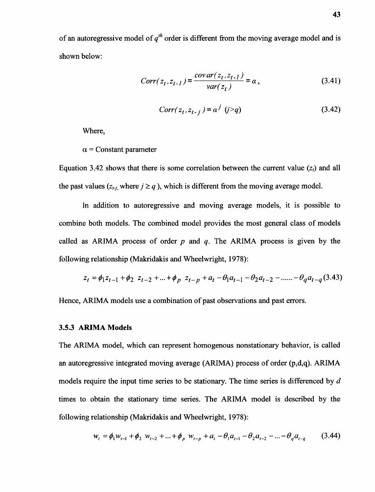
Corr(zt ,zt _ i )= =a,var(zt )
Corr(zt ,zt _ i )= al (j>q)
covar(zt,zt_i)(3.41)
(3.42)
43
of an autoregressive model of q th order is different from the moving average model and is
shown below:
Where,
a = Constant parameter
Equation 3.42 shows that there is some correlation between the current value (zt) and all
the past values (zt_j , where] which is different from the moving average model.
In addition to autoregressive and moving average models, it is possible to
combine both models. The combined model provides the most general class of models
called as ARIMA process of order p and q. The ARIMA process is given by the
following relationship (Makridakis and Wheelwright, 1978):
zt Oizt-i +02 zt _2 +...+ Op p at -19iat _ 1 - 02at_2 - - gat _q (3.43)
Hence, ARIMA models use a combination of past observations and past errors.
3.5.3 ARIMA Models
The ARIMA model, which can represent homogenous nonstationary behavior, is called
an autoregressive integrated moving average (ARIMA) process of order (p,d,q). ARIMA
models require the input time series to be stationary. The time series is differenced by d
times to obtain the stationary time series. The ARIMA model is described by the
following relationship (Makridakis and Wheelwright, 1978):
Wt = 01 Wt-1 + 02 Wt-2 • + 0 p Wt-p at -01a1-1 -92 111-2 - ••• - eg al-q (3.44)
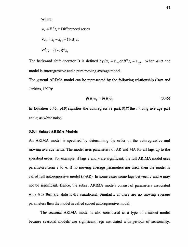
44
Where,
w, = V d zt = Differenced series
Vz, = z, — z t _ i = (1-B) z,
V d z, = (1- B) d z,
The backward shift operator B is defined by Bz, = zi_ i or Bin z t = z t _ff, . When d=0, the
model is autoregressive and a pure moving average model.
The general ARIMA model can be represented by the following relationship (Box and
Jenkins, 1970):
0(B)wt = 0(B)at (3.45)
In Equation 3.45, 0(B) signifies the autoregressive part, 0(B) the moving average part
and at as white noise.
3.5.4 Subset ARIMA Models
An ARIMA model is specified by determining the order of the autoregressive and
moving average terms. The model uses parameters of AR and MA for all lags up to the
specified order. For example, if lags 1 and n are significant, the full ARIMA model uses
parameters from 1 to n. If no moving average parameters are used, then the model is
called full autoregressive model (F-AR). In some cases some lags between 1 and n may
not be significant. Hence, the subset ARIMA models consist of parameters associated
with lags that are statistically significant. Similarly, if there are no moving average
parameters then the model is called subset autoregressive model.
The seasonal ARIMA model is also considered as a type of a subset model
because seasonal models use significant lags associated with periods of seasonality.

45
Seasonal models can be AR, MA or ARMA. The general notation of a seasonal ARIMA
model with both seasonal and non seasonal factors is ARIMA (p,d,q) x (P,D,Q),. The
term (p,d,q) gives the order of the non-seasonal part and the term (P,D,Q) gives the order
of the seasonal part. The value of s represents the number of observations in a seasonal
cycle and D represents the degree of seasonal differencing used. The seasonal
differencing combined with non-seasonal differencing is represented by the following
relationship (Box and Jenkins, 1970):
Wt = (1— B) d (1— B s ) D zt (3.46)
Where,
s = Number of observations in a seasonal cycle
D = Degree of seasonal differencing
Hence, the general form of a seasonal ARIMA model is represented by the following
relationship (Box and Jenkins, 1970):
0(B) (1)(B s )Wt = 60(B)0(B s )at (3.47)
Where,
J(B s )= Seasonal autoregressive part
O(B s ) = Seasonal moving average part
The value of D can vary based on the seasonality and is suggested by the significance of
the lags in the autocorrelation and partial autocorrelation diagram. In some cases, both
seasonal and non-seasonal parameters may be present, where significant lags may be
present due to seasonal data and some non recurring non-seasonal data.

46
3.5.5 Residual Analysis and Performance of Models
A residual is defined as the difference between observed and predicted values of the time
series. The residuals are plotted against time over the total period of fit and used to
evaluate the overall fit of the time series model. The prediction errors are required to be
random for the time series model to be adequate. If the mean residual is close to zero, it is
concluded that there is no forecast bias in the model (Chatfield, 2000). A large individual
residual suggests an outlier in the data.
In addition to the time series of residuals, an ACF plot of residuals describes the
linear relationship between successive residuals. Hence, the ACF plot of residuals also
provide an indication of whether the model has a good fit and indicates any remaining
structure not explained by the model. For a good prediction model, the expected values of
rk should be zero or close to zero. The statistical significance of the individual rk can be
examined to determine if any exceed 2 / .NP—V (where N is the number of sample
observations) in magnitude.
The chi-square test statistic of the residuals indicates whether the residuals are
uncorrelated or have additional information that could be explained by a more complex
model. This is an approximate statistical test of the hypothesis that residuals are
uncorrelated up to a given lag. The p-values of correlation between errors are also
determined using the significance level of 95%. If the p-value is less than 0.005 then the
hypothesis is rejected and concluded that the residuals are correlated and the fitted model
is not adequate.
The performance evaluation of the bus arrival time prediction model is
determined by evaluating Mean Absolute Relative Error (MARE) and Mean Absolute

47
Percentage Error (MAPE). MARE values are used to determine the performance of the
arrival time prediction model, where the average of difference between the observed
arrival time and the predicted arrival time is determined. However, MAPE values are
used to determine the performance of the travel time prediction model. The following
equations state the relationships for these measures:
ActualValuei— ForecastValueil
MARE — 1 =1
(3.48)n
MAPE _ 1=1
ActualValuei —ForecastValuei x 100
ActualValuei(3.49)
n
Where,
1= Individual bus trips
n= Total number of bus trips
3.6 Discrete and Finite State Delay Propagation Model
3.6.1 Finite State Markov Chain
A Markov chain is a stochastic process where an outcome of an event depends only on
the present state rather than past states. The process can be visualized using a simple
pictorial representation as shown in Figure 3.1, where the process moves from state to
state If the state of the system is represented by s and m is the number of states, (i, j =
1, m) then the nth order transition probabilities for a Markov process is denoted by
p ii(n) as defined by the following relationship:
pii (n)=P(xi+n =si lxi =s1 )
(3.50)

48
The transition probabilities py(n) denote the probability that the process goes from
state i at the th step to state j after n steps or transitions. For a homogeneous Markov
process, transition probabilities, pu(n), do not depend on n and can be relaxed to pu . In a
non-homogeneous Markov process, py changes over n. With a slight modification in the
probability structure used for a homogeneous Markov process, a non- homogeneous
Markov process can be obtained. Quite often / and n are substituted as time periods
instead of steps. In that case, when the probability relating the next period's state to the
current state does not change over time, then the process is called a stationary Markov
chain.
Figure 3.1 Discrete and finite state Markov chain with "m" delay states and delaystates as "On-time, Late and Early".

49
The number of states is assumed to be finite. The transition probability matrix
{Ai } is a square matrix of size m x m and is represented as follows:
••• Pim
P = (13y} = (3.51)
`pmt • • • Pim /
Where,
P = {p ii } = Transition matrix
P11' pmm = Transition probabilities from state 1 to m (0 py 1)
m = Number of States.
In Equation 3.51, pH represents the probability that given the system is in state 1, it will
move to state 1 after one step or one period of time. All the entries in the transition
probability matrix are nonnegative and the entries in each row must sum to unity, which
is represented as follows (Winston, 1993):
E P( xn = si I P(xn_ i = si )) =1 (3.52)
E = 1(Vi)
(3.53)= 1
A Markov process is completely defined by its transition probability matrix and
initial state or an initial probability vector (Taylor and Karlin, 1998). The initial
probability vector gives the probabilities for the various possible starting states and is
represented by Po. Based on an initial probability vector, the probability of the process to
be in state sj after n steps is determined the by following relationship (Kemeny and Snell,
1976):
Pn Pn--1.P(n) (3.54)

50
Where,
Pn= Transition probabilities after n steps.
Pn-] = Initial probability vector.
P(n) = Transition matrix between the steps n-1 and n.
By successive application of Equation 3.54, the probability of the process after n steps is
given by the following relationship:
Pn ponP(i)
(3.55)i=1
For a homogeneous n-step Markov process, where P(n) are the same for each step or
time-period, Equation 3.55 can be written as follows:
Pn=PO.P(1)n (3.56)
Similarly, for a non-homogeneous n-step Markov process, Equation 3.56 can be modified
as follows:
Pn= Po.P(1).P(2)...P(n) (3.57)
Where,
P(1), P(2), ..P(n) = Transition matrix between steps 0 and 1, 1 and 2,...and steps
n-1 and n.
Pn= Transition probabilities after n steps.
In Equation 3.57, instead of using the power of matrix (Pt, individual matrices P(1),...
P(n) are used to reflect the heterogeneous Markov process.

51
3.6.2 Estimation of Transition Probabilities
Transition probabilities are easily estimated if observations are available over time on
individual transitions. Transition probabilities can then be determined as a ratio of the
number of observed delay states to the total number of delay states. Anderson and
Goodman (1957) developed a maximum likelihood estimation of stationary transition
probabilities by the following method:
Maximizing Pn Po .P(1) P(n) (3.58)
Subject to,
py 0
E =1i= 1
Hence,
nilfiy = (Vi )
Iny
j
(3.52)
Where,
py = Transition probabilities between states i and j of the matrix P(n).
n ii = Number of events where state changed from i to j.
The estimate ofpy is the ith row and jth column of the table of ny 's divided by the
sum of the ith entry in the table (Anderson and Goodman, 1957). This method counts the
frequency of an event (transition from state i to state j) that occurred in the past and
determines the probability (p i.) of that event divided by the total number of i events. The
limitation of the maximum likelihood of estimation of transition probabilities is that, if
any event is zero, then the p ;; for that particular event is zero.

52
3.6.3 Application of Markov Chain to Predict Delay
To apply a Markov chain model to predict bus delays at downstream stops, possible delay
states at the upstream stop have to be determined. In this research, the term "Delay" is
used generically to refer to the "Early", "On-time", and "Late" arrival of a bus at a
time-point. Delay is defined as the difference between the observed and scheduled arrival
time of a bus at a time-point. A constant value "w" is introduced, which is transit agency
may use as a threshold value to define if the bus is "Late" or "Early". Since, the value of
"w" may vary among transit agencies, in this research a value of "w" is assumed as 5
minutes. Bus delays are defined by the following relationships:
Di = Oi — Si (3.60)
Late = Di > w,( w > 0)
Ontime = (-w +w )
Early = Di < —w
Where,
D, = Bus arrival delay at time-point i.
0, = Observed arrival time of bus at time-point i
S, = Scheduled arrival time of bus at time-point i
w = Constant in minutes (Based on a transit agency's policy to define Early, On-
time and Late bus arrivals)
In Equation 3.60, the bus is "Late" if the delay (D,) is greater than w=5 minutes.
If the delay is between -5 and +5 minutes, the bus is "On-time". Similarly, if the delay is
less than w=-5 minutes, then the bus "Early". For each trip, the delay (D,) is determined
using Equation 3.6. In this research, the delay states (si, s2, s3, s„,) represent possible

53
ranges of bus delay between any two time-points. The value of m depends on the number
of delay states between each pair of time-points. In this research, the possible delay states
are limited to On-time, Early, Late. More detailed delay states, such as {-10, -8,....., 0,
....,+8, +10) minutes can be used. However, to incorporate more detailed delay states
requires a large number of samples corresponding to each delay state.
The transition probabilities between delay states are represented by a transition
matrix of size (m x m) with elements {p,d, where each element represents the conditional
probability that given a current bus is delayed s, at time-point i, the bus will be delayed si
at time-point i+1. For each combination of time-points, separate transition matrices are
determined represented by ((Ado], ••• ••• ••••, {pidi_1 3 ). As the bus traverses downstream,
the delay at the downstream time-point (i+1) is predicted using the transition matrix
{p,j},,,+] and the initial probability vector at i. To determine the delay at the downstream
time-points, Equation 3.55 is modified as follows:
do = Po.P(1)....P(n).sT
(3.61)
Where,
= Delay at the nth time-point.
ST = Transpose of delay states.
Po = Initial probability vector with the form {0, 1, 0, ... 0} or E pi =1 at 0th
i=i
time-point.
The nature of the bus delay propagation to downstream time-points can be
homogeneous or heterogeneous. Homogeneous propagation refers to an equal amount of
delay propagated to downstream time-points from an upstream time-point. This is

54
assumed to occur if the distances between downstream time-points are similar in length
and traffic characteristics to the preceding time-points. In contrast to homogenous
propagation, a heterogeneous propagation of delay occurs when the links connecting
time-points differ in length and traffic characteristics. In homogeneous delay propagation,
the transition matrix between time-points is assumed to be identical. However, for
heterogeneous delay propagation, the transition matrix differs for each set of time-points
as a result of differences in the length and traffic behavior on the links. Markov chain
models can be used to model either homogeneity or heterogeneity of delay propagation
between any combinations of time-points.
To determine the delay at the immediate downstream time-point 1 measured from
time-point 0 (origin), Equation 3.61 is modified as follows:
di = P0 .(P(1)) 1 .sT (3.62)
i P// • • • P/m
V i Si \
di = Po (3.63)
Piii I • • • Pim i0,1 ism i
Similarly, based on homogeneous propagation of delay between time-points 0 and 1 and
1 and 2, the delay at time-point 2 measured from the time-point 0, is predicted by using
the following relationship:
d2 = p0. (po i)2 .sT (3.64)
(
Pi] Phn N2 / ■
Si
d2 = PO (3.65)...\Pm 1 Pmm 10,1 'ini 1

d2 = Po .P(1).P( 2 ).1 (3.66)
• • • Pim(
Pi i • - • Pim B SI
(3.67)
— • Pmm
d2 = Po
) 0,1■Pm1 )1,20m i•••
Pnlm
55
Hence, by the successive application of Equations 3.62 and 3.63, the delay at any
downstream time-point can be determined from any upstream time-point assuming a
homogeneous propagation of delay.
However, assuming two corresponding links are homogeneous in characteristics
may not be realistic. In most instances, links have variable lengths, traffic volumes and
number of traffic signals. In such a situation, a heterogeneous Markov chain is used by
obtaining different transition probability matrices between the corresponding time-points.
For example, to predict the delay at time-point (i=2) from origin (i=0), Equation 3.61 is
modified as follows:
Where,
r P11 • • • Pimi \P11 • • - Pim
= Transition probabilities between
P MI • • • P Mtn 1 0 , 1 P1111 • • • PM M /1 , 2
time-points 0, 1 and 1, 2.
By expanding Equation 3.61, the delay at the nth time-point from any kth (k<n) time-point
can be determined by the following relationships:
do = po. ( p )n—k .5,7•
(3.68)
do = Po•P(k )••••P(n).s T (3.69)

56
Equation 3.68 assumes that links between time-points k and n have similar
characteristics or are homogeneous and Equation 3.69 assumes that links between time-
points k and n have dissimilar characteristics, or are heterogeneous. The difference
between Equations 3.68 and 3.69 is that in Equation 3.68, the transition probability
matrix is successively powered by an integer. In Equation 3.69, individual transition
probabilities between any two time-points are multiplied.
CHAPTER 4
CASE STUDY ANALYSIS
4.1 Introduction
In this chapter, an explanation of the bus route selected as a case study is provided. The
structure of the source data, which is gathered from an APC system installed on the buses
running along the route, is also explained. The chapter provides a discussion of the
variables required to successfully develop time series models for bus arrival time
prediction. In addition, an analysis of the bus delay propagation pertaining to the case
study is performed. The bus arrival time algorithm and the results obtained for the case
study is presented in subsequent chapters.
4.2 Description of a Case Study
The data for this research was obtained from buses equipped with a GPS based APC
system and operated in the State of New Jersey. Such buses run along a number of
routes, one of which is route number 62, which runs from downtown Newark in Essex
County to Woodbridge Center Mall in Middlesex County. The bus route map is shown in
Figure 4.1.
The one-way trip time from Newark's Penn Station to Woodbridge Center Mall is
about 1 hour 40 minutes. The bus travels through different land uses such as a downtown
location in the city of Newark, industrial areas at Port Newark/Elizabeth, and suburban
locations in towns of Metuchen, Edison and Woodbridge. The route is also comprised of
different types of roadways such as, urban arterials, state highways and rural roads. The
57

NEWARK PENN STATIO
NWK AIRPORT TERM C
SAINT GEORGES AVE. & WOOD AVE.
BROAD ST. & BRANFORD PL
NWK AIRPORT TERM
BROAD ST. & W JERSEY ST
58
route comprises of roadways with a variety of traffic volumes and signal density. These
conditions have a direct effect on bus travel time. The bus route consists of 135 stops
with 14 designated time-points.
Figure 4.1 GIS diagram of bus route 62 with time-points.

59
4.3 APC Data Structure
The data collected from the APC system consists of 7 months of data from June to
December 2002. In the database used in this research, information about the bus stop is
available only if the bus actually stops there. If the bus did not stop at a bus stop because
of the absence of boarding or alighting passengers, then no information is recorded. The
APC system provides the following information about the existing condition of the bus:
Location of bus in geographical coordinates (latitude and longitude);
Scheduled arrival and departure time at time-points only;
- Observed arrival and departure time at time-points and bus stops;
Time- points where the bus stopped;
Dwell time at bus stops, door open and close time; and
Number of passengers boarding and alighting.
The information about a bus trip provided in the data source is shown in Table
4.1, which consists of data for a single trip. In the table, "Stop ID" represents the
identification given to each stop along the bus route. The door open time and close time
at the corresponding stop is provided with the corresponding scheduled arrival time.
Since Stop ID's 30, 40 and 80 are not time-points, the scheduled arrival times for these
stops are not available. In addition, the bus trips are classified in the database into seven
different time of day periods based on schedule start time of the trip. The classification of
time of day is presented in Table 4.2.. These times indicate the scheduled trip start time.

60
Table 4.1 Sample AVL/APC Data of a Single Bus Trip
ScheduledOpen Close Stop ScheduledStart Ons Offs
TimeTime Time ID Time
08:05:00 080118 080506 10 8:05 AM 15 008:05:00 080812 080814 40 0 008:05:00 080929 081006 50 8:09 AM 9 108:05:00 081121 081231 60 1 108:05:00 081313 081322 70 1 108:05:00 082052 082100 0 0 108:05:00 082350 082429 140 8:25 AM 3 408:05:00 082640 082647 0 0 208:05:00 082915 082930 150 8:28 AM 2 108:05:00 083140 083212 160 8:31 AM 1 608:05:00 084018 084023 190 0 1
Table 4.2 Classification of Time of Day
Time of Day Hour of Day
Early Morning 4:00 - 7:00Morning Peak 7:00 - 9:00Late Morning 9:00 — 12:00Mid-day 12:00 —14:00Early Afternoon 14:00 —16:00Afternoon Peak 16:00 — 18:00Evening 18:00 - 21:00
4.4 Spatial Analysis of Link Travel Time
The preliminary analysis of the bus travel time data consists of obtaining travel time
values from the system's database to arrange the data in a time series. This process
consists of arranging the travel time data so that it corresponds to identified links and
61
time periods. The observed travel time between two time-points is the difference between
the door open time at the following stop and the door close time at the preceding stop.
The door close and open times are obtained from the APC system installed in the bus.
In this research, the coefficient of variation of travel times for each link is
determined to study the characteristics of the links along the bus route. It is presumed that
the coefficient of variation of links along the bus route varies based on the land use of the
link and not the link length. It is assumed that a higher coefficient of variation is observed
at urban and downtown locations and a lower coefficient of variation is observed at rural
and highway locations along the bus route.
For normal (Gaussian) distributions, the coefficient of variation (c v) measures the
relative scatter or variation in the data with respect to the mean and is expressed as the
ratio of standard deviation to mean. A higher coefficient of variation is associated with a
higher variability of travel times and a lower coefficient of variation is associated with a
lower variability of observed travel times.
The coefficient of variation of travel time between links and time-points was
found to vary depending on the length of the link and traffic characteristic along the link.
These characteristics of the link are influenced by the link location (central business
district (CBD), suburban or rural location). Table 4.3 provides the coefficient of variation
of travel time at different links of the study bus route after averaging the travel times. For
a link within the CBD (link 10-50), the coefficient of variation is higher than that of a
link located outside the CBD (link 50-140), in spite of the fact that the length of the link
50-140 is longer than the link 10-50. This finding concurs with the fact that highway
segments have less fluctuation in volume and speed than road segments located in the
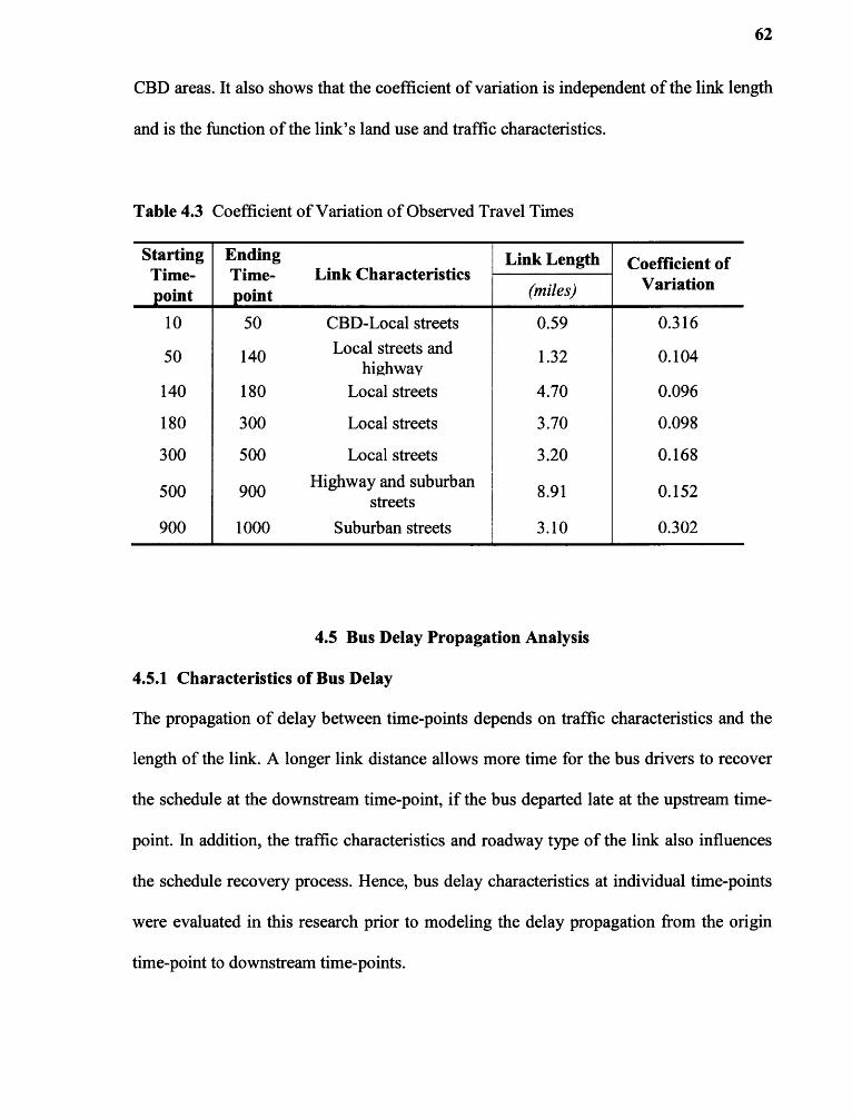
62
CBD areas. It also shows that the coefficient of variation is independent of the link length
and is the function of the link's land use and traffic characteristics.
Table 4.3 Coefficient of Variation of Observed Travel Times
StartingTime-point
EndingTime- Link Characteristicspoint
Link Length Coefficient ofVariation(miles)
10 50 CBD-Local streets 0.59 0.316
50 Local streets and140highway
1.32 0.104
140 180 Local streets 4.70 0.096
180 300 Local streets 3.70 0.098
300 500 Local streets 3.20 0.168
500 Highway and suburban900 streets 8.91 0.152
900 1000 Suburban streets 3.10 0.302
4.5 Bus Delay Propagation Analysis
4.5.1 Characteristics of Bus Delay
The propagation of delay between time-points depends on traffic characteristics and the
length of the link. A longer link distance allows more time for the bus drivers to recover
the schedule at the downstream time-point, if the bus departed late at the upstream time-
point. In addition, the traffic characteristics and roadway type of the link also influences
the schedule recovery process. Hence, bus delay characteristics at individual time-points
were evaluated in this research prior to modeling the delay propagation from the origin
time-point to downstream time-points.
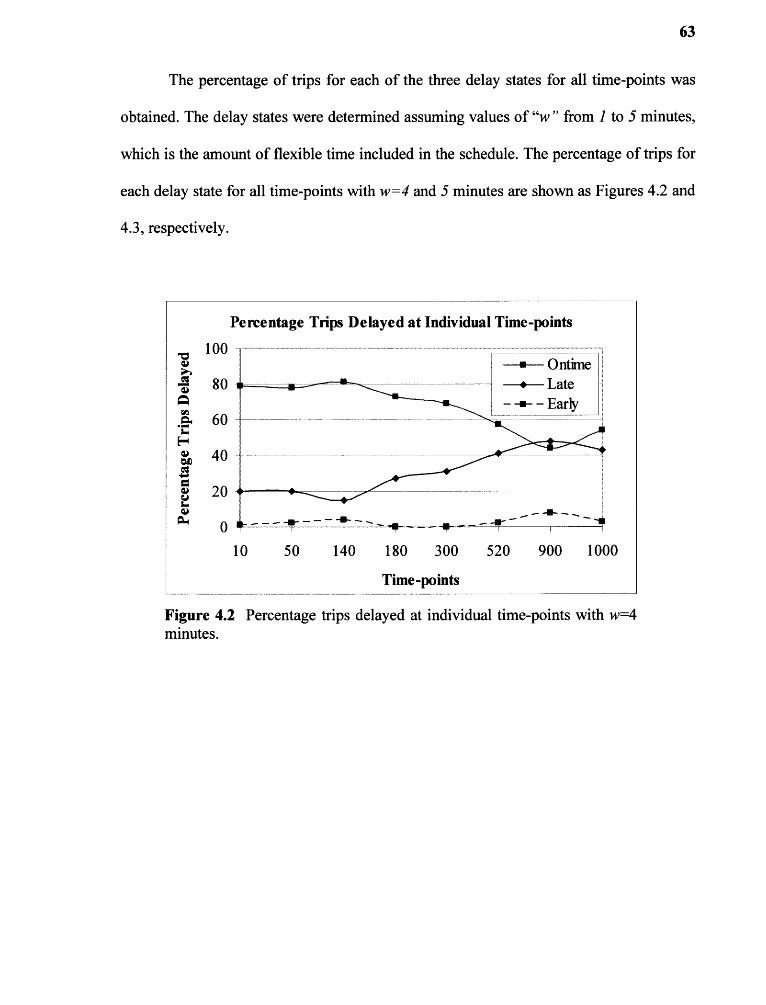
Percentage Trips Delayed at Individual Time-points
100
Ctlaa
z60 .-6
asago 40
2 •ca 0as064
10 50 140 180 300 520 900 1000
() IF- AR- -11-
OntimeLate
- - Early
go
Time-points
63
The percentage of trips for each of the three delay states for all time-points was
obtained. The delay states were determined assuming values of "w " from 1 to 5 minutes,
which is the amount of flexible time included in the schedule. The percentage of trips for
each delay state for all time-points with w=4 and 5 minutes are shown as Figures 4.2 and
4.3, respectively.
Figure 4.2 Percentage trips delayed at individual time-points with w=4minutes.
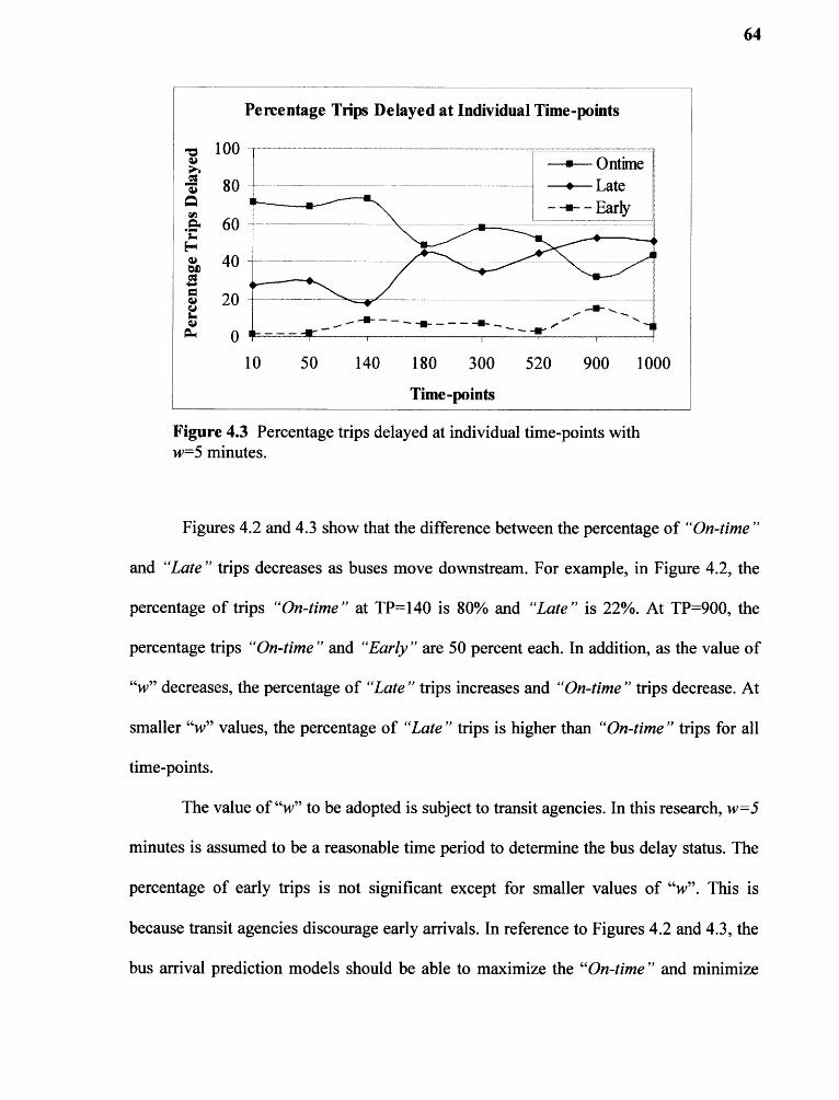
--6-- Ontime--.-- Late- -*- - Early
Percentage Trips Delayed at Individual Time-points
v 100 -a)ata) 80Az 60a.,...1.
E.*460
4-1= 20at
Ai
10 50 140 180 300 520 900 1000
-111F---
..-- .........0'
- iT I
Time-points
64
Figure 4.3 Percentage trips delayed at individual time-points withw=5 minutes.
Figures 4.2 and 4.3 show that the difference between the percentage of "On-time"
and "Late" trips decreases as buses move downstream. For example, in Figure 4.2, the
percentage of trips "On-time" at TP=140 is 80% and "Late" is 22%. At TP=900, the
percentage trips "On-time" and "Early" are 50 percent each. In addition, as the value of
"w" decreases, the percentage of "Late" trips increases and "On-time" trips decrease. At
smaller "w" values, the percentage of "Late" trips is higher than "On-time" trips for all
time-points.
The value of "w" to be adopted is subject to transit agencies. In this research, w=5
minutes is assumed to be a reasonable time period to determine the bus delay status. The
percentage of early trips is not significant except for smaller values of "w". This is
because transit agencies discourage early arrivals. In reference to Figures 4.2 and 4.3, the
bus arrival prediction models should be able to maximize the "On-time" and minimize

65
the "Late" percentage of trips at each time-point. Figures 4.2 and 4.3 also show the
"trouble" time-points, where buses have higher probability of arriving late and being
unable to adequately recover the schedule.
4.5.2 Non-Homogenous Delay Propagation
Bus delay propagation to downstream time-points can be either homogeneous or
heterogeneous. The type of delay propagation is important in modeling the delay
propagation. Regardless of whether the delay propagation is homogeneous or
heterogeneous, a Markov chain model can be devised. Homogeneous propagation refers
to an equal amount of delay propagated to downstream time-points from an upstream
time-point. This is assumed to occur if the downstream time-points are equidistant in
length and traffic characteristics are similar along the route. In contrast to homogenous
propagation, heterogeneous propagation of delay occurs when the links connecting time-
points differ in length and traffic characteristics. In this research, the study bus route
travels through links variable in length and traffic characteristics. Based on Table 4.4,
which shows the links connecting time-points for the route under study are variable in
length and land-use, it can be assumed that the links connecting individual time-points
vary in traffic characteristics as well.

66
Table 4.4 Linear Regression Slopes Between TP=10 andDownstream Time-points
DownstreamTime-points
Regression Slope(Intercept = 0)
50 0.966
140 0.312
180 0.454
300 0.413
500 0.896
900 0.651
1000 1.086
The homogeneity or heterogeneity of delay propagation along a bus route can be
determined by comparing the slopes of a linear regression of delay at individual time-
points. The linear regression of the delay at the origin time-point is the independent
variable (x) and the delay at any downstream time-point (y) is the dependent variable
observed during previous trips. Regression slopes less than 1 suggest that the delay at the
downstream time-point (y) is reduced as the bus travels from one time-point to another.
Hence, the slope of the resulting linear regression represents the schedule recovery by bus
drivers and the delay propagation at a particular time-point along the link. The slopes are
plotted for each link along the entire bus route. If the slopes are decreasing or increasing
towards the destination time-point at a uniform rate, the links along the bus route can be
termed homogeneous.
A linear regression was performed to determine the linear relationship of the bus
delays at the origin time-point (TP=10) and each of the remaining downstream time-
points. Figure 4.4 shows the slopes of the regression model relating the delay at the

0
50 140 180 300 520 900 1000
Downstream Time-points
1.2
1 11
0.8 —1:1.1
0.6 — ■0.4 —
0.2
Linear Regression Slopes between TP-10 andDownstream TPs
67
origin time-point to the delay at each downstream time-point. For example, the slope at
TP=50 is greater than 1 and much higher than the slope at TP=140. This relationship
shows that buses are less able to recover their schedule at TP=50 compared to TP=140.
Figure 4.4 also shows that the slopes are not decreasing or increasing uniformly towards
the destination time-point. Hence, it could suggest that the delay propagation is not
homogeneous between individual links and the transition probabilities of each link are
not the same. The existence of homogeneous delay propagation would have generated a
uniformly decreasing or increasing curve.
Figure 4.4 Linear regression slopes between TP=10 and downstreamtime-points.
Ideally, if there is a delay at the origin time-point, delays at the downstream time-
points should gradually reduce and reach a negligible value at the destination time-point.
This means bus drivers should be able to fully recover the schedule by the time the bus
reaches the destination time-point. However, from Figure 4.4 it is observed that for the
68
study route bus drivers are not able to fully recover the schedule at the destination time-
point (TP=1000), though some amount of schedule recovery occurs at TP=140, as
indicated by the decreasing slope from TP=50 to TP=140. An important observation from
Figure 4.4 is that the schedule recovery process varies at each link between time-points
because of the variable length of link and traffic characteristics. Hence, it would not be
appropriate to assume that delay would propagate homogeneously towards downstream
time-points.
The schedule recovery process shown in Figure 4.4 consists of all the samples (all
available bus trips), and no temporal differentiation has been made. For example, a single
slope is used to represent the schedule recovery process between the links. However, the
amount of schedule recovery may vary during different time periods such as peak and off
peak hours. Figure 4.4, suggests that the schedule recovery process varies at each link as
shown by the varying amount of regression slopes.

CHAPTER 5
PREDICTION OF BUS TRAVEL TIME
5.1 Introduction
The bus travel times are predicted independent of the delay propagation model, which is
based on Markov chains. The bus travel time prediction model is then included as a part
of a combined model with delay propagation model to predict bus arrival times. In this
chapter, the selection of appropriate autoregressive time series models to predict bus
travel time is presented. In addition, the parameter estimates and performance measure of
the models are also presented. Full autoregressive, seasonal and subset autoregressive
models were then developed for individual links that would be used to predict bus travel
times. Finally, comparisons between the autoregressive models and the more complex
models were performed to select the most appropriate model.
5.2 Graphical Analysis
Bus travel time series were obtained for each bus stop along the bus route for different
times of the day. The time series starts from Monday 5 AM and extends to Sunday 8 PM,
as shown in Figures 5.1 and 5.2. Figure 5.1 shows bus travel time between TP=10 and
TP=50 and Figure 5.2 shows bus travel time between TP=50 and TP=140. Each point in
the graph is the mean bus travel time for different days at the same time of day. The
vertical axes in the time series graphs represent the bus travel time between stops. The
horizontal axis represents the day of week.
69

2
10
1
Monday Tuesday Wednes Thursday Friday Saturday
Time of Day
Figure 5.1 Time series plot of observed travel time for link 10-50.
70
Figure 5.2 Time series plot of observed travel time for link 50-140.

71
The above time series provided some insight into the variability, trend and cyclic
behavior of bus travel time. A distinct observation was that the time series graphs were
very similar for all links in terms of trend and variability during time of day. On each day
of the week, morning and evening peak hours showed higher travel times than other
times of day. However, the peaks varied on different days. The graphs showed that the
mean travel time increased from early morning towards the morning rush to afternoon
peak and decreased thereafter, which is a very typical observation of traffic condition.
The graphs showed higher travel time on Monday with slowly decreasing travel times for
the remainder of the week.
The highest peaks in Figures 5.1 and 5.2 are primarily associated with the
afternoon peak period. The afternoon peaks are usually followed by a smaller value of
travel time in the evening. Similar trends in time series were obtained for both links 10-
50 and 50-140. It was observed that the cyclic behavior is more prominent on link 10-50
than on link 50-140. This is because link 50-140 has a lower coefficient of variation and
the link consists of highway sections with a lower probability of recurring congestion.
5.3 Autocorrelation Functions
The sample ACF/PACF plot and model fit plot were obtained for each time series. The
ACF and PACF plots differ by link and by time of day. The ACF plot showed
statistically significant lags at the peak periods, but also showed seasonality extending
five days starting from Monday through Friday. Hence, in addition to full autoregressive
models, subset/seasonal autoregressive models were also considered to determine bus

72
travel time models using significant lags only and comparing these models with full
autoregressive models.
The ACF and PACF plots indicated a full autoregressive model with lag 7 for
most of the links. Hence, the time series fitted autoregressive parameters with p= 7. The
ACF plot of link 10-50 is shown in Figure 5.3. For link 50-140, the ACF plot is similar to
the ACF plot of link 10-50. Lags are shown in the horizontal axis and the autocorrelation
(rk) is shown on the vertical axis. It can be seen from Figure 5.3 that all the parameters of
the lags from 1 to 7 were not significant. The significant lags are 2, 5 and 7. These lags
correspond to the morning peak, early afternoon and evening periods. The full
autoregressive model was developed based on the above observations.
Figure 5.3 Autocorrelation plot of observed travel time for link 10-50.

73
The presence of seasonality in all time series was also checked with ACF and
PACF plots. The time series of link 10-50 showed peaks at lags 7 and 14, but the peaks
die down exponentially as shown in Figure 5.3. Hence, there is strong seasonality in this
link. From the ACF and PACF plots, it is clear that the peaks at periods 2 and 7, which
correspond to morning and afternoon peak, were more prominent. Using these
observations for all links, the parameters were selected for full, subset and seasonal
models.
5.4 Historical Average and Exponential Smoothing Models
The selection of the appropriate number of periods (n) used in the historical average
model and the smoothing factor (a) in the exponential smoothing model was made
iteratively. Mean absolute percent error (MAPE) was used as the performance measure to
compare the performance of the model for different values of n and a. The higher the
value of (n) in the historical average model, the smoother the fit of the curve resulting in
larger reduction of the overall MAPE of the prediction model. In the exponential
smoothing model, the lower value of a gives a smoother model and reduces the overall
MAPE. The smoother curve means the variance in the original time series is not well
described by the model.
From Table 5.1, the overall MAPE for link 10-50 is below 20% and 10% for the
rest of the links except for link 300-500. The MAPE values observed for all the links are
consistent with the coefficient of variation of travel times at these links. For example, the
coefficient of variation for link 50-140 was lower than the coefficient of variation for link
10-50. Similarly, the MAPE of link 50-140 is lower than that of link 10-50.

74
Table 5.1 MAPE for Historical Average and Single ExponentialSmoothing of Observed Bus Travel Time
LinksHistorical ExponentialAverage Smoothing
a10-50 20.81 3 20.03 0.4
50-140 5.60 3 5.75 0.3
140-180 4.35 5 5.55 0.1
180-300 5.21 5 7.24 0.1
300-500 12.50 6 13.40 0.3
500-900 7.50 6 7.46 0.1
900-1000 7.55 6 8.00 0.1
Figures 5.4 and 5.5 show estimates of bus travel times using the historical average
and exponential smoothing models and the observed travel time for links 10-50 and 50-
140, respectively. The MAPE achieved for both models did not vary significantly. The
estimated travel times obtained from both models are also similar. However, the
smoothing models are not able to correctly estimate the peak values during certain time-
periods. These peak values are the results of re-occurring peak conditions along the bus
route. For this reason, historical average and exponential smoothing models are not
suitable to predict bus travel times in links where there is substantial peaking of bus
travel time data.

Observed Values
Historic Average
Exponential Smoothing8
Tuesday Wednesday Thursday Friday Saturday
6
2
0
Monday
Time of Day
Time Series of Observed Travel Time at Link 10-50
10
Figure 5.4 Smoothing model diagram for link 10-50.
Time Series of Observed Travel Time at Link 50-140
15
14aE 13
g 12
11
Es 10E;
9
8
Observed Value
-Historic Average
Exponential Smoothing
Monday Tuesday Wednesday Thursday Friday Saturday
Time of Day
75
Figure 5.5 Smoothing model diagram for link 50-140.

76
5.5 Minimum AIC and Parameter Estimates
The minimum value of the AIC is used to select the appropriate number of "p"
parameters in the full autoregressive model. In addition, the Mean Absolute Percentage
Error (MAPE) of the model is also used to evaluate the performance of the model. The
MAPE and AIC were determined for different "p" parameters for two links, 10-50 and
50-140, as shown in Figures 5.6a and b. In both figures, there is a sudden drop in the AIC
close to the optimum value of "p". The sudden drop in the AIC is also consistent with the
drop in the MAPE. This confirms that the model selected based on minimum AIC
consistently shows minimum MAPE as well. The process of selecting the final models
using minimum values of MAPE and AIC were used for all links.
The number of parameters used in developing the full autoregressive model is
always equal to the number of time-periods (time of day) in a day minus one time period.
For example, in link 10-50, the minimum MAPE and AIC occurred at p=6. The number
of time periods within any day for link 10-50 is 7 demonstrating the relationship between
the optimum p value and the number of time periods within the day. Similarly, for links
140-180 and 180-300, the morning peak trips were not available, which resulted in one
less time period and one less parameter in the full autoregressive model. Hence, the
number of autoregressive parameters was 5 (p=5).
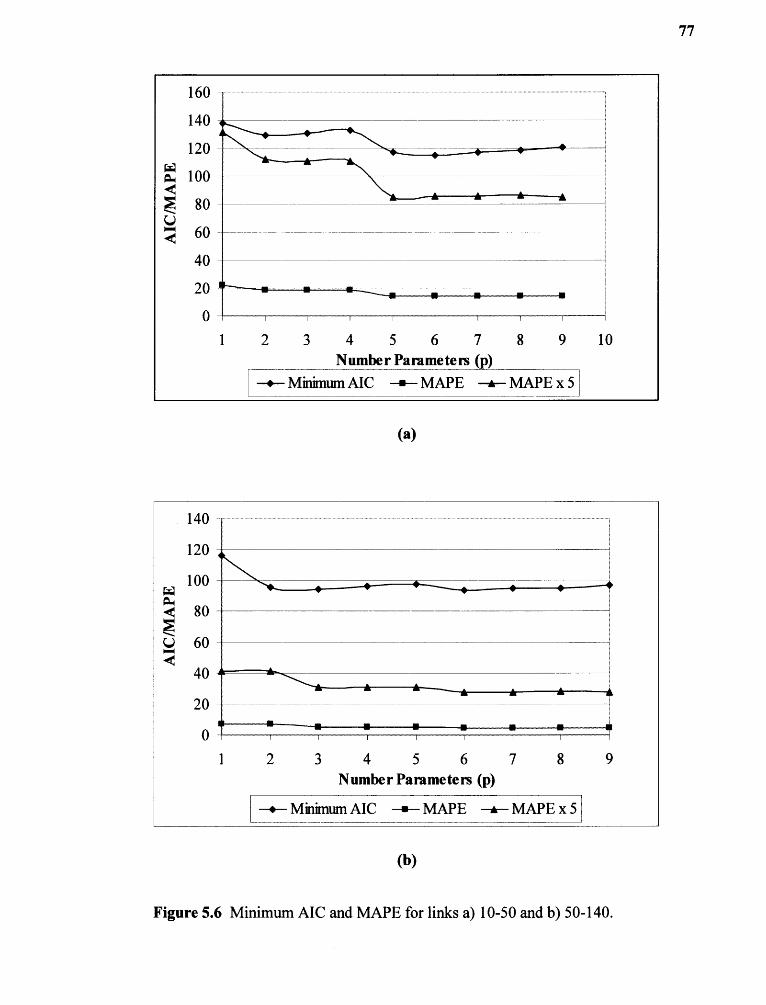
160
140
120 •
100
80
60
40
20
0
1
2 3 4 5 6 7 8 9
1 0Number Parameters (p)
Minimum AIC MAPE MAPE x 5
(a)
77
140
120
100 4N1/4 •
4e 80
U 60
40
20 • ■ ■ ■ ■ 1111 ■ ■
0
1 2 3 4 5 6 7 8 9Number Parameters (p)
Minimum AIC MAPE MAPE x 5
(b)
Figure 5.6 Minimum AIC and MAPE for links a) 10-50 and b) 50-140.

78
5.6 Full Autoregressive Model
The analysis using full autoregressive models showed that higher orders ofp resulted in a
MAPE around 15% for link 10-50 and less than 10% for the rest of the links as shown in
Table 5.2, with the exception of link 140-180 which has a MAPE of 10.78%. These
values are a significant improvement from the historical average and exponential
smoothing models. The AIC for all links listed in Table 5.2 are minimum values. Hence,
the order of autoregressive models is optimum. The results also showed that single order
of differencing is appropriate for the full autoregressive models.
Table 5.2 MAPE for Full AR Model of Observed Bus Travel Time
Link MAPE Model AIC
10-50 14.30 (6,1,0) 115.14
50-140 4.61 (6,1,0) 93.71
140-180 10.79 (5,1,0) 160.77
180-300 4.72 (5,1,0) 98.91
300-500 6.53 (6,1,0) 148.56
500-900 4.88 (6,1,0) 184.51
900-1000 7.48 (6,1,0) 134.05
Table 5.3 provides the estimated parameters for link 10-50 with the standard
error, t-value and p-values. The p-values for all parameter estimates are significant at a
95% confidence level with one parameter having a p-value of 0.0540. The full
autoregressive prediction model for link 10-50 can be written as follows:
zt = —0.632zt_i —0.751zt_2 —0.677zt_3 — —0.315zt_6 +at (5.1)
Or,

79
(1+0.632B 1 +0.751B2 +0.677B3 + +0.315B6 )zt =at (5.2)
Table 5.3 Parameter Estimates of Full AR Model for Link 10-50
Model = F-AR (6,1,0)
Parameter Estimate StandardError t Value Pr > Iti
col -0.63262 0.15875 -3.99 <.0001
92 -0.75123 0.14151 -5.31 <.0001
93 -0.67767 0.17677 -3.83 0.0001
94 -0.51271 0.17540 -2.92 0.0035
-0.76909 0.14209 -5.41 <.0001
96 -0.31504 0.16348 -1.93 0.0540MAPE 14.30%
The estimated and observed travel times for links 10-50 and 50-140 using full
autoregressive models are shown in Figures 5.7 and 5.8, respectively. The peaks
predicted by the full autoregressive model are similar to the observed peak values, unlike
the estimate predicted by the historical average and smoothing models. These figures also
include 95% upper and lower confidence limits of the predicted travel time. The observed
travel times are well within the confidence limits.
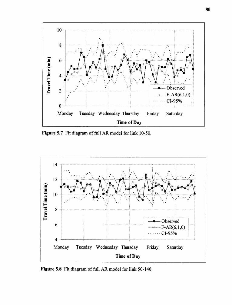
,,•,.
ObservedF -AR(6, 1 ,0) CI-95%
Monday Tuesday Wednesday Thursday Friday Saturday
Time of Day
14
12
10
• . s
• - ,
4Monday Tuesday Wednesday Thursday Friday Saturday
Time of Day
Figure 5.7 Fit diagram of full AR model for link 10-50.
Figure 5.8 Fit diagram of full AR model for link 50-140.
80

81
5.7 Seasonal and Subset Autoregressive Model
The results of fitting a seasonal autoregressive model on the time series are shown in
Table 5.4. For all links, the order of seasonal models used was 7 based on 7 time periods
in a given day. It was assumed that the seasonality is repeated each day. However, the
order of seasonality of links 140-180 and 180-300 was 6 because the number of time
periods available was 6 in a day. For link 10-50, the MAPE obtained was similar to that
of the full autoregressive model. However, the MAPE was higher for the seasonal model
compared to the full autoregressive model for all other links. This demonstrates that a
seasonal model may not be suitable for predicting bus travel times. Figures 5.9 and 5.10
show observed and predicted bus travel times for links 10-50 and 50-140, respectively.
Table 5.4 MAPE for Seasonal AR Model of the ObservedBus Travel Time
Links MAPE Model AIC
10-50 18.40 (1,1,0)(1,1,0)7 111.85
50-140 6.27 (1,1,0)(1,1,0)7 88.21
140-180 14.15 (1,1,0)(1,1,0)6 145.60
180-300 5.97 (1,1,0)(1,1,0)6 88.63
300-500 6.68 (1,1,0)(1,1,0)7 123.53
500-900 7.25 (1,1,0)(1,1,0)7 168.44
900-1000 8.93 (1,1,0)(1,1,0)7 118.48

Observed(1,1,0)(1,1,0)7 CI-95%
Monday Tuesday Wednesday Thursday Friday Saturday
Time of Day
16
14,
, •
,' •• .
:s., •
12 --•:-.'
•.- ,•• •. ..0.,
, •
I •1 0
bser ved6 (1,1,0)(1,1,0)7
CI-95%4
Monday Tuesday Wednesday Thursday Friday Saturday
Time of Day
82
Figure 5.9 Fit diagram of seasonal AR model for link 10-50.
Figure 5.10 Fit diagram of seasonal AR model for link 50-140.
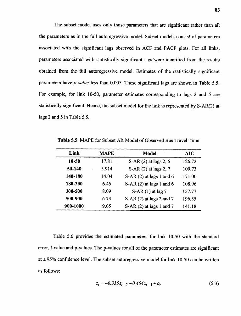
83
The subset model uses only those parameters that are significant rather than all
the parameters as in the full autoregressive model. Subset models consist of parameters
associated with the significant lags observed in ACF and PACF plots. For all links,
parameters associated with statistically significant lags were identified from the results
obtained from the full autoregressive model. Estimates of the statistically significant
parameters have p-value less than 0.005. These significant lags are shown in Table 5.5.
For example, for link 10-50, parameter estimates corresponding to lags 2 and 5 are
statistically significant. Hence, the subset model for the link is represented by S-AR(2) at
lags 2 and 5 in Table 5.5.
Table 5.5 MAPE for Subset AR Model of Observed Bus Travel Time
Link MAPE Model AIC
10-50 17.81 S-AR (2) at lags 2, 5 126.72
50-140 5.914 S-AR (2) at lags 2, 7 109.73140-180 14.04 S-AR (2) at lags 1 and 6 171.00
180-300 6.45 S-AR (2) at lags 1 and 6 108.96
300-500 8.09 S-AR (1) at lag 7 157.77500-900 6.73 S-AR (2) at lags 2 and 7 196.55
900-1000 9.05 S-AR (2) at lags 1 and 7 141.18
Table 5.6 provides the estimated parameters for link 10-50 with the standard
error, t-value and p-values. The p-values for all of the parameter estimates are significant
at a 95% confidence level. The subset autoregressive model for link 10-50 can be written
as follows:
zt = —0.335 zt_2 —0.464zt_5 +at (5.3)

84
Or,
(1+0.335B 2 +0.464B5 )zt =at (5.4)
Table 5.6 Parameter Estimates of Subset AR Model at Lags 2 and 5for Link 10-50
S-AR (2) at lags 2 and 5
Parameter Estimate StandardError t Value
CO2
5
-0.33568
-0.46432
0.12556
0.12821
-2.67
-3.62
MAPE 17.81%
Pr > It!
0.0075
0.0003
Figures 5.11 and 5.12 show estimated and observed bus travel times for links 10-
50 and 50-140, respectively. For the time series, the peaks predicted by the model do not
fit the observed pattern as the observed peaks seem to lag behind the predicted peaks as
seen in the historical average and exponential smoothing model. Hence, subset
autoregressive models may not appropriately model the observed bus travel time during
peak periods.
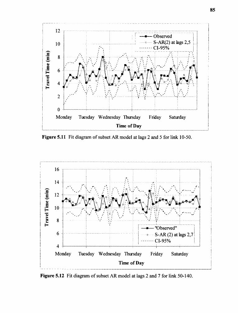
85
ObservedS-AR(2) at lags 2,5
CI-95%
Tuesday Wednesday Thursday Friday Saturday
Time of Day
, •' • t '• •
•••
16
14
12
10
"Observed"S-AR (2) at lags 2,7CI-95%
4
Monday Tuesday Wednesday Thursday Friday Saturday
Time of Day
Figure 5.11 Fit diagram of subset AR model at lags 2 and 5 for link 10-50.
Figure 5.12 Fit diagram of subset AR model at lags 2 and 7 for link 50-140.

86
5.8 Comparison of Autoregressive Models
The analysis showed higher order full autoregressive models resulted in an MAPE of
around 15% for link 10-50 and 4.5% for link 50-140. This is compared to the historical
and smoothing exponential models which resulted in MAPE values of 20.81 and 5.61.
The MAPE for the full autoregressive model are lower than the MAPE obtained from
historical average, exponential smoothing models, seasonal and subset autoregressive
models.
The results also showed that the appropriate model "p" parameter was 6 except
for links 140-180 and 180-300, for which it was 5. In most cases, lags pertaining to peak
hours were more significant than lags of other periods. The peaks predicted by the full
autoregressive model are similar to the observed peak values.
For seasonal models there was a mixed response, since some links showed strong
seasonality and some did not. For example, the time series for link 10-50 showed peaks at
lags 7 and 14, but the peaks die down exponentially. For link 50-140, the peaks at lags 2
and 5 were statistically significant followed by statistically significant peaks at 10 and 14.
However, there was not much increase in MAPE using seasonal models in comparison to
full autoregressive models.
The subset model focuses on using individual significant parameter estimates
rather than all the parameter estimates as in the full autoregressive model and consists of
parameters associated with the significant lags only. The peaks predicted by the model do
not fit the observed pattern as the observed peaks seem to lag behind the predicted peaks
as in historical average and exponential smoothing model.
87
In conclusion, full autoregressive models perform better than seasonal and subset
models. The presence of seasonality is not significant except in a few cases, because of
the larger variation in observed travel times. Hence, seasonal and subset autoregressive
models do not improve the overall MAPE above the performance of the full
autoregressive model.
5.9 Cross Validation of Full AR Models
It is important to determine if full autoregressive models would perform differently when
the time series is shortened. If the MAPE of the full autoregressive model is very
different for the time series with a smaller amount of data, then the ability of the model to
consistently give similar MAPE may be questionable. The ability of the full
autoregressive model to predict bus travel time using variable lengths of time series was
validated by splitting the time series data.
The full autoregressive model for the entire week (Monday, Saturday) of
time series data was split and evaluated using only the first four days (Monday, ......,
Thursday). Due to the fact that the number of samples was reduced, the parameter
estimates for the model using the time series for the entire week and the parameter
estimates for the model using a time series consisting of the first four days differed even
though the full autoregressive model order was the same. In addition to the consistency of
models, the analysis also showed the individual model's ability to provide reasonable
forecast with a smaller number of time series data.
To compare the model's performance due to the reduced sample and to test the
ability of the models to forecast the following two days of data, MAPE for individual
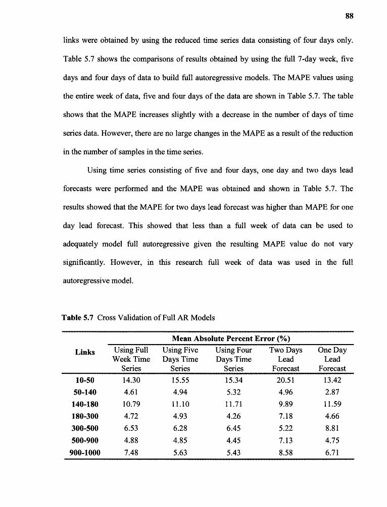
88
links were obtained by using the reduced time series data consisting of four days only.
Table 5.7 shows the comparisons of results obtained by using the full 7-day week, five
days and four days of data to build full autoregressive models. The MAPE values using
the entire week of data, five and four days of the data are shown in Table 5.7. The table
shows that the MAPE increases slightly with a decrease in the number of days of time
series data. However, there are no large changes in the MAPE as a result of the reduction
in the number of samples in the time series.
Using time series consisting of five and four days, one day and two days lead
forecasts were performed and the MAPE was obtained and shown in Table 5.7. The
results showed that the MAPE for two days lead forecast was higher than MAPE for one
day lead forecast. This showed that less than a full week of data can be used to
adequately model full autoregressive given the resulting MAPE value do not vary
significantly. However, in this research full week of data was used in the full
autoregressive model.
Table 5.7 Cross Validation of Full AR Models
Links
Mean Absolute Percent Error (%)Using FullWeek Time
Series
Using FiveDays Time
Series
Using FourDays Time
Series
Two DaysLead
Forecast
One DayLead
Forecast
10-50 14.30 15.55 15.34 20.51 13.42
50-140 4.61 4.94 5.32 4.96 2.87
140-180 10.79 11.10 11.71 9.89 11.59
180-300 4.72 4.93 4.26 7.18 4.66
300-500 6.53 6.28 6.45 5.22 8.81
500-900 4.88 4.85 4.45 7.13 4.75
900-1000 7.48 5.63 5.43 8.58 6.71

CHAPTER 6
PREDICTION OF BUS DELAY
6.1 Introduction
This chapter describes the use of a Markov process to determine the propagation of bus
delay and provides a basis for using bus delay in the prediction of bus arrival times. The
propagation of bus delay based on a Markov process has been explained in this chapter.
Based on an assumption of either homogeneous or heterogeneous traffic conditions
between the links, the transition probabilities are predicted and compared with observed
transition probabilities. Predicted transition probabilities obtained using heterogeneous
traffic conditions between links were close to the observed transition probabilities.
6.2 Estimation of Transition Probabilities
The formulation of a Markov process to determine bus delay propagation requires the
estimation of transition probabilities of delay states between time-points. To determine
transition probabilities of delay states between time-points, the number of observed delay
states were obtained and classified as "On-time", "Late" and "Early" at each time-point.
The transition probabilities were obtained using the following relationship:
,m E (1,3},k E (LK} (6.1)
Where,
m = Total number of delay states = 3
ny = Number of events where state changed from i to ./
89

90
k = Number of time-points
The delay states and the representative transition matrix is shown as follows:
Pij
nrl 1
P21
31
P12
P22
P32
P13
P23
P33
ontime — ontime
late — ontime
early — ontime
ontime —late
late —late
early — late
ontime — early \
late — early
early — early ,,
(6.2)
Each po represents the probability of being in a delay state at the downstream time-
point when the upstream time-point has a delay state of (i). For example, pi represents
the probability that the delay state at the downstream time-point is "On-time", given the
delay state at the origin time-point (TP=10) is also "On-time".
For each combination of origin time-point (TP=10) delay state and downstream
time-point delay state, transition probabilities (py) were determined using Equation 6.1
and are shown in Table 6.1. In addition, the transition probabilities of delay states
between consecutive time-points were determined as shown in Table 6.2. The observed
transition probabilities for the remaining links are provided in Appendix A. In Table 6.1,
the probability of the bus being "On-time" at a downstream time-point is higher if the
bus is "On-time" at the origin time-point. The "Early" delay state has lower frequency
than other delay states. This is because transit agencies discourage drivers to reach time-
points early.
The largest probability in any transition matrix occurs when the upstream time-
point has "On-time" delay state and the corresponding delay state at the downstream
time-point is also "On-time". This shows that most of the trips on the study route reach
time-points "On-time" when buses reach the upstream time-points "On-time". However,
this probability decreases as the bus moves downstream, as seen from the lower transition
probabilities for time-points 180 to 1000 in Table 6.1.

Table 6.1 Observed Transition Probabilities Between TP=10 and DownstreamTime-points Based on Maximum Likelihood Estimation
On-time Late Early DownstreamTP
Total SampleSize
On-time 0.876 0.119 0.005 50 215
Late 0.107 0.893 0.000
Early 0.000 0.500 0.500
On-time 0.905 0.048 0.048 140 274
Late 0.595 0.380 0.025
Early 0.500 0.000 0.500
On-time 0.653 0.327 0.020 180 86
Late 0.622 0.378 0.000
Early 0.000 0.000 0.000
On-time 0.762 0.201 0.037 300 271
Late 0.596 0.385 0.019
Early 0.333 0.000 0.667
On-time 0.715 0.252 0.033 500 204
Late 0.436 0.526 0.038
Early 0.333 0.333 0.333
On-time 0.657 0.224 0.119 910 114
Late 0.383 0.553 0.064
Early 0.000 0.000 0.000
On-time 0.638 0.313 0.050 1000 266
Late 0.431 0.559 0.010
Early 0.000 0.500 0.500
91

Table 6.2 Observed Transition Probabilities Between Time-points Based onMaximum Likelihood Estimation
On-time Late Early UpstreamTime-point
DownstreamTime-point
On-time 0.876 0.119 0.005 10 50
Late 0.107 0.893 0.000
Early 0.000 0.500 0.500
On-time 0.922 0.026 0.052 50 140
Late 0.353 0.647 0.000
Early 0.000 0.000 1.000
On-time 0.777 0.215 0.008 140 180
Late 0.050 0.900 0.050
Early 0.667 0.000 0.333
On-time 0.865 0.125 0.010 180 300
Late 0.146 0.854 0.000
Early 0.200 0.200 0.600
On-time 0.790 0.189 0.021 300 500
Late 0.132 0.868 0.000
Early 0.250 0.000 0.750
On-time 0.898 0.020 0.082 500 910
Late 0.105 0.895 0.000
Early 0.000 0.500 0.500
On-time 0.887 0.113 0.000 910 1000
Late 0.000 1.000 0.000
Early 0.545 0.182 0.273
92
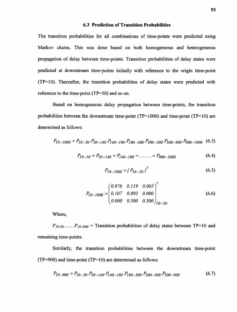
93
6.3 Prediction of Transition Probabilities
The transition probabilities for all combinations of time-points were predicted using
Markov chains. This was done based on both homogeneous and heterogeneous
propagation of delay between time-points. Transition probabilities of delay states were
predicted at downstream time-points initially with reference to the origin time-point
(TP=10). Thereafter, the transition probabilities of delay states were predicted with
reference to the time-point (TP=50) and so on.
Based on homogeneous delay propagation between time-points, the transition
probabilities between the downstream time-point (TP=1000) and time-point (TP=10) are
determined as follows:
P10-1000 = P10-50•P50-140•P140-180.P180-300•P300-500•P500-900•P900-1000 (6.3)
P10-50 = P50-140 = P140-180 = = P900-1000 (6.4)
P10-1000 = (P10-50)7 (6.5)
(0.876 0.119 0.005\7
o— l000 = 0.107 0.893 0.000 (6.6)
\0.000 0.500 0.500 ji0_50
Where,
P 1 0-56 •••• P 1 0-1 000 = Transition probabilities of delay states between TP=10 and
remaining time-points.
Similarly, the transition probabilities between the downstream time-point
(TP=900) and time-point (TP=10) are determined as follows:
P10-900 = P10-50•P50-140•P140-180•P180-300•P300-500•P500-900 (6.7)

94
P10-900 ={ Pij }ro-5,9 (6.8)
(0.876 0.119 0.005 6
P10-900 = 0.107 0.893 0.000
(6.9)
0.000 0.500 0.500 10_50
Equation 6.3 is based on the assumption that the delay at TP=1000 due to the delay at
TP=10 is a function of delay at individual links and these delays are homogeneously
propagated as shown in Equation 6.4.
Unlike Equation 6.3, by assuming that propagation of delay is heterogeneous, the
predicted delay state at downstream time-point (TP=1000) with reference to the origin
time-point (TP=10) is obtained by following relationships:
P10-1000 = P10-50.P50-140.P140-180.P180-300 1
900-1000
P10-50 P50-140 P900-1000
0.876 0.119 0.005 1 '0.887 0.113 0.000\
Pi o-1000 = 0.107 0.893 0.000
0.000 1.000 0.000
(6.12)
\ 0.000 0.500 0.500110_50 0 545 0.182 0.273)900-1000
Using Equations 6.10 and 6.12, the po 's for all the downstream time-points were
determined with reference to time-point (TP=10). The results of the predicted transition
probabilities at individual time-points with reference to the origin time-point (TP=10) are
shown in Table 6.3. The predicted transition probabilities for all the links are presented in
Appendix B.

Table 6.3 Predicted Transition Probabilities Between TP=10 andDownstream Time-points
On-time Late Early DownstreamTP
On-time 0.876 0.119 0.005 50
Late 0.107 0.893 0.000
Early 0.000 0.500 0.500
On-time 0.849 0.099 0.050 140
Late 0.484 0.580 0.005
Early 0.176 0.323 0.500
On-time 0.698 0.272 0.028 180
Late 0.354 0.611 0.034
Early 0.486 0.329 0.184
On-time 0.650 0.325 0.024 300
Late 0.403 0.573 0.024
Early 0.506 0.378 0.115
On-time 0.563 0.405 0.032 500
Late 0.400 0.573 0.026
Early 0.478 0.424 0.097
On-time 0.548 0.390 0.062 910
Late 0.519 0.534 0.045
Early 0.474 0.437 0.087
On-time 0.520 0.463 0.017 1000
Late 0.397 0.590 0.012
Early 0.468 0.507 0.023
95

96
6.4 Comparison of Transition Probabilities
The transition probabilities of delay states between origin TP=10 and the remainder of
the downstream time-points were predicted first by using Equation 6.9 and assuming a
homogeneous propagation of delay and then by using Equation 6.10 and assuming a
heterogeneous propagation of delay between time-points. The predicted transition
probabilities were then compared with the observed values, which are shown in Figure
6.1, assuming a homogeneous propagation of delay, and Figure 6.2, assuming a
heterogeneous propagation of delay.
Figure 6.1 a consists of predicted and observed transition probabilities of "On-
time" delay state between time-points TP=10 and 50, based on homogeneous propagation
of delay. Figure 6.1b consists of predicted and observed transition probabilities of "Late"
delay state between time-points TP=10 and 50. The comparison between predicted and
observed transition probabilities of "Early" delay states are not shown because of their
large prediction error. This is because the sample size of "Early" delay states is very
small and in most cases zero.
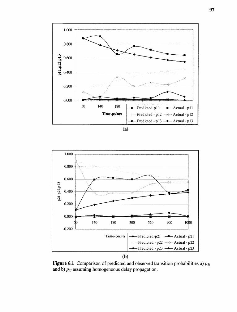
1.000
0.800
M7,.." 0.600
c. 0.400
0.200
0.00050 140 180
Time-points
Predicted11 Actual 11-p
Predicted - p 12
Predicted 13
—a-- - p
- - Actual - p 12
Actual 13—)K— - p - p
0.000(
50 140 180 300 520 900 1000
-0.200
Time -points Predicted-p21 Actual - p21Predicted - p22 Actual - p22
---o— Predicted - p23 Actual - p23
T.
1.000
0.800
0.600eqi
0.400
CL
ca.
0.200
(a)
(b)Figure 6.1 Comparison of predicted and observed transition probabilities a)and b) p2j assuming homogeneous delay propagation.
97

98
In Figure 6.1 a, three comparisons are made for transition probabilities p11, p12 and
p13. The transition probability pi i refers to the probability of the delay state going from
"On-time" to "On-time". Transition probability p12 refers to the probability that the delay
state goes from "On-time" to "Late". For pii, the predicted probability is a smooth curve
similar to a negative exponential curve. This is because of the nth power of a matrix for
homogeneous propagation (Kemeny and Snell, 1979). The predicted probability is
relatively close to the observed probability for this case. For p12, the predicted
probability that the bus goes from being "On-time" to being "Late" increases as the
distance to the time-point increases.
Figure 6.1b compares the observed and predicted transition probabilities p21, p22,
and p23. The transition probability p21 refers to the probability that the delay state goes
from "Late" to "On-time". Transition probability p23 refers to the probability that the
delay state goes from "Late" to "Early". For p21, the predicted probability that the delay
state goes from "Late" to "On-time" increases as the distance to the time-point increases.
This observation indicates that schedule recovery has a higher chance of occurring at
further time-points. Differences between the predicted and observed probabilities seem
to be larger for the first time-point and for the last two time-points. For p22, the predicted
probability that the delay state for the bus goes from "Late" to "Late" decreases as the
distance to the time-point increases. This observation reflects the condition that schedule
recovery is likely to occur as the distance increases, and therefore, the likelihood of the
bus remaining in a "Late" state decreases as the distance to the time-point increases. For
P23, the predicted probability that the delay state for the bus goes from "Late" to "Early"
is very similar to the observed probability.
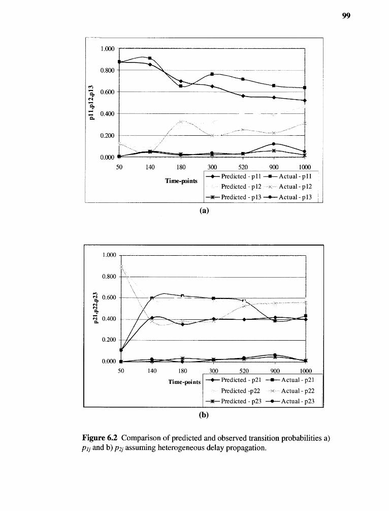
300 520 900 1000 Predicted - p 11 —s-- Actual - p 11Predicted - p12 - Actual - p12
—0— Predicted - p13 Actual - p13
Time-points
(a)
Ti me-pointsPredicted - p21
Actual - p21
Predicted -p22
Actual - p22
—*-- Predicted - p23
Actual - p23
(b)
Figure 6.2 Comparison of predicted and observed transition probabilities a)pi; and b) p2j assuming heterogeneous delay propagation.
99
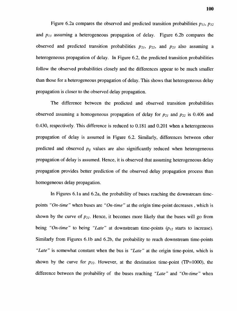
100
Figure 6.2a compares the observed and predicted transition probabilities p11, p12
and p13 assuming a heterogeneous propagation of delay. Figure 6.2b compares the
observed and predicted transition probabilities p21, p22, and p23 also assuming a
heterogeneous propagation of delay. In Figure 6.2, the predicted transition probabilities
follow the observed probabilities closely and the differences appear to be much smaller
than those for a heterogeneous propagation of delay. This shows that heterogeneous delay
propagation is closer to the observed delay propagation.
The difference between the predicted and observed transition probabilities
observed assuming a homogeneous propagation of delay for p21 and p22 is 0.406 and
0.430, respectively. This difference is reduced to 0.181 and 0.201 when a heterogeneous
propagation of delay is assumed in Figure 6.2. Similarly, differences between other
predicted and observed p ly values are also significantly reduced when heterogeneous
propagation of delay is assumed. Hence, it is observed that assuming heterogeneous delay
propagation provides better prediction of the observed delay propagation process than
homogeneous delay propagation.
In Figures 6.1a and 6.2a, the probability of buses reaching the downstream time-
points "On-time" when buses are "On-time" at the origin time-point decreases , which is
shown by the curve of p11. Hence, it becomes more likely that the buses will go from
being "On-time" to being "Late" at downstream time-points (p12 starts to increase).
Similarly from Figures 6.1b and 6.2b, the probability to reach downstream time-points
"Late" is somewhat constant when the bus is "Late" at the origin time-point, which is
shown by the curve for p22. However, at the destination time-point (TP=1000), the
difference between the probability of the buses reaching "Late" and "On-time" when

101
the bus is "Late" at the origin time-point, represented by p22 and 1321, respectively, is
smaller than at other downstream time-points. This shows that bus drivers try to recover
the "Late" bus to reach the destination time-point "On-time".
6.5 Performance Evaluation of Markov Model
A chi-square goodness of fit test was employed to test whether the observed transition
probabilities are close to the transition probabilities predicted from the Markov process.
If the chi-square statistic is less than the table value, then the hypothesis that the observed
data are the outcomes of the predicted Markov process is true. The chi-square model for
(r-1) degrees of freedom is given by the following relationship (Lee and Judge, 1973):
2X(r-1) =E N( - SO2 / S7i (6.13)
Where,
r = Number of delay states
N= Sample size
yi = Observed proportion in state i
yi = Predicted proportion in state I
The chi-square values obtained using Equation 6.13 determined for homogeneous
and heterogeneous delay propagation are shown in Table 6.4. These values are compared
against the chi-square values of 5.991 for a 95% confidence interval and 2 degrees of
freedom. From Table 6.4, the calculated chi-square values for the transition probabilities
predicted with reference to origin time-point (TP=10) assuming heterogeneous delay
propagation are less than 5.991 except for links 10-180, 10-300 and 10-1000. This shows

102
that the predicted transition probabilities are close to the observed transition probabilities
and they are outcomes of the Markov process.
However, the calculated chi-square values for the transition probabilities
predicted with reference to origin time-point (TP=10) assuming homogeneous delay
propagation are higher than 5.991 for all links This shows that the predicted transition
probabilities determined assuming homogeneous delay propagation are not close to the
observed transition probabilities and they may not be an outcome of the Markov process.
Table 6.4 Comparison of Predicted and Observed Transition Probabilities
UpstreamTP
DownstreamTP
x2 (Calculated)(Homogeneous Delay)
p11....p13 P21...P23 P31...P33
10 50 0.000 0.000 0.000*10 140 9.796 16.938 28.00010 180 1.369 6.732 0.000*10 300 13.984 9.328 19.86210 500 18.852 6.699 9.03110 900 8.687 15.427 0.000*10 1000 5.002 1.993 93.667
(* indicates zero sample size)
UpstreamTP
DownstreamTP
x2 (Calculated)(Heterogeneous Delay)
P21...P23 P31...P33
10 50 0.000 0.000 0.00010 140 2.356 3.677 0.91610 180 2.032 5.513 9.00010 300 3.685 5.366 15.39410 500 5.203 4.482 5.11010 900 3.150 0.413 2.00010 1000 4.724 0.203 109.508

CHAPTER 7
BUS ARRIVAL TIME COMPUTATIONS
7.1 Introduction
This chapter presents the results of bus arrival time predictions using delay propagation
only, autoregressive models only, and a combination of both methods. For comparison
purposes, the MARE was obtained for the delay propagation algorithm and the combined
algorithm as mentioned in Section 3.3.
7.2 Prediction of Bus Arrival Time Using Delay Propagation
The transition probabilities were predicted as explained in Chapter 3 and 6 assuming
heterogeneous traffic conditions, as the assumption of heterogeneous transition
probabilities produced results closer to the observed probabilities than the transition
probabilities assuming homogeneous conditions. For individual trips, the predicted delay,
obtained by using the Markov process at a time-point was compared with the observed
delay and the MARE was calculated. As the difference between the observed and
predicted delay is the same as the difference between the observed and predicted arrival
time, the difference in delay was used to determine the reliability of the Markov process.
The prediction of the bus arrival time uses scheduled arrival time and the predicted delay,
which are shown by the following relationships:
A i = SATi + PDi (7.1)
0D i = AT i — SAT i (7.2)
Prediction Error = AT i — A i = ATi — SATi — PD i = 0D i — PD i (7.3)
103

Ei ODD — PDi IMARE =
k
Where,
ATi = Observed arrival time at time-point i = Door open time at i
Ai = Predicted arrival time at time-point i using Markov process
SAT i = Scheduled arrival time at i
OD i = Observed delay at i
PD i = Predicted delay at i using Markov process
MARE values show the capability of the Markov delay model to reasonably
predict the bus arrival time at various downstream time-points. MARE values were
determined for each combination of time-points and are shown in Table 7.1.
Table 7.1 MARE of Bus Arrival Time at Time-points Using Markov Model Only
DestinationOrigin 50 140 180 300 500 900 100010 3.38 3.22 3.3 3.24 3.24 3.27 3.2750 2.71 2.43 2.04 3.15 3.33 2.82140 2.94 2.25 2.77 3.17 2.43180 1.48 2.67 4.02 4.14
Table 7.1 consists of MARE values obtained for selected route segments. The
MARE values move decreases till time-point TP=500. After TP=500, the MARE values
do not show a definite trend. This shows that the prediction capability of the Markov
model increases when a time-point that is being used to predict the bus arrival time is
located near the destination time-point. For example, while predicting delay at TP=300,
the MARE is smaller when the origin is TP=140 compared to the MARE when the origin
104
(7.4)

105
TP=10. This is shown by the MARE value for TP=10 which is higher than that for
TP=140. This result shows that the MARE decreases and the prediction accuracy
increases as the bus arrival time is predicted closer to the destination time-point.
The MARE values are about 3 minutes when the origin TP=10, 50 and 140.
However, the MARE values slightly exceeded 4 minutes for the origin time-points
TP=180 and 300. The MARE value of 3.2 minute for link 10-50 is inadequate
considering the average travel time of 5.0 minutes. However, considering the average
travel time between time-points 10 and 1000 is 90 minutes, the 3 minute MARE is a
highly desirable accuracy of predicting bus arrival times.
The benefits of using delay propagation to predict bus arrival time and relay delay
information to passengers at downstream time-points are determined by comparing the
probability distributions of predicted and observed delay at time-points. The probability
distribution in the form of a histogram and normal curve of the observed and predicted
delay for link 10-50 is shown as Figure 7.1. The comparison of probability distributions
between predicted and observed delay for the rest of the links is presented in Appendix E.
In Figure 7.1, the left graph is the histogram and normal curve for the observed
delay and the right graph is for the predicted delay. The graph for the predicted delay has
a steeper curve than the curve for the observed delay. Also, the spread of absolute values
of predicted delay is smaller than the spread for the observed delay, which indicates
smaller mean and standard deviation for the predicted delay. Smaller mean and standard
deviation of predicted delay indicates a lower probability of prediction error when
providing the predicted delay information to passengers. Also, the prediction model did
not produce very high prediction error, which shows that the prediction model is robust.

106
Delay(min)
Frequency (trips) Frequency (trips)
(a) (b)
Figure 7.1 Histogram and normal curve of absolute values of (a) observedand (b) predicted delay at link 10-50.
7.3 Bus Travel Time Prediction Using Autoregressive Models
The appropriate full autoregressive models for each combination of time-points were
determined to predict bus travel times using the optimum AIC method having the
minimum MAPE. The full autoregressive models for all the links are presented in Table
7.2, including MAPE and AIC values. In addition to MAPE, MARE values were
determined for each combination of time-points, which are presented in Figure 7.2.

Table 7.2 Final Full AR Models of Bus Travel Time
Link MAPE Model AIC10-50 14.30 (6,1,0) 115.14
10-140 9.70 (2,1,0) 181.1310-180 7.40 (6,1,0) 221.6410-300 7.39 (7,1,0) 255.6510-500 6.58 (6,1,0) 270.0310-900 4.59 (6,1,0) 270.6610-1000 4.45 (7,1,0) 273.9650-140 4.61 (6,1,0) 93.7150-180 4.41 (6,1,0) 175.2550-300 6.62 (6,1,0) 233.7950-500 6.02 (6,1,0) 247.0950-900 5.57 (6,1,0) 278.8450-1000 10.61 (6,1,0) 279.59140-180 10.79 (5,1,0) 160.77140-300 9.39 (6,1,0) 226.54140-500 9.39 (6,1,0) 226.55140-900 4.38 (6,1,0) 261.22140-1000 5.41 (6,1,0) 275.02180-300 4.72 (5,1,0) 98.91180-500 7.16 (3,1,0) 214.51180-900 5.32 (7,1,0) 265.55180-1000 5.70 (6,1,0) 280.28300-500 6.53 (6,1,0) 148.56300-900 5.42 (6,1,0) 227.55300-1000 5.59 (6,1,0) 252.70500-900 4.88 (6,1,0) 184.51500-1000 10.90 (6,1,0) 299.59900-1000 7.48 (6,1,0) 134.05
107

108
OriginTime-points
X10
—§1— 50
140
180
—4E-- 300
500
0
50
140 180 300 500 900
1000
Destination Time -points
Figure 7.2 MARE values of bus travel time at time-points using full autoregressivemodel.
Figure 7.2 shows the MARE values obtained from different upstream time-points
to downstream time-points using multiple trips. The MARE of the predicted travel time
using full autoregressive models varied linearly as the bus traversed downstream. The
MARE increased from 1 minute while predicting bus travel time to time-point (TP=50) to
5 minutes for travel time at time-point (TP=1000). However, the MARE values at time-
point (TP=1000) from all the other upstream time-points remained constant at around 5
minutes. Considering that the average travel time from the origin time-point (TP=10) to
time-point (TP=1000), which is 1.5 hours, the MARE of 5 minutes can be considered an
acceptable result.

109
7.4 Combined Model of Autoregressive and Delay Propagation Models
Using the combined algorithm, which includes a full autoregressive time series model to
predict bus travel time and a Markov process to predict bus delay at time-points, the
arrival times of bus at individual time-points were predicted. The bus travel times
between time-points were predicted using a full autoregressive model based on historic
bus travel time data. The predicted delay propagation at individual downstream time-
points was determined using the Markov model based on heterogeneous delay
propagation between time-points.
The difference between the predicted and the observed arrival times were
compared using MARE values, as shown in Figure 7.3. The MARE values increased as
the prediction horizon extended to downstream time-points, reaching close to 6 minutes
at the destination time-point (TP=1000). This observation is valid for all origin time-
points, as shown by each curve corresponding to origin time-points in Figure 7.3. In
addition, MARE values decreased as the time-point from where the prediction is being
performed is closer to destination time-points. For example, the curve for time-point
(TP=50) is lower than the curve for the time-point (TP=10). This shows that there is
reduction in MARE values when bus arrival time prediction is done from the time-point
closer to the time-point for which the bus arrival time is being predicted. Hence, it can be
concluded that the prediction accuracy increases as the reference time-point is moved
closer to the time-point where bus arrival time prediction is being predicted.

110
Figure 7.3 MARE values at time-points using combined model.
The effect of combining bus delay propagation with the full autoregressive model
to predict bus arrival times is shown by comparing the MARE values of predicted and
observed arrival times using only the full autoregressive models, as presented in
Figure 7.4.

111
Figure 7.4 MARE values using full autoregressive model only.
To better compare Figures 7.3 and 7.4, the curves obtained in both figures were
combined and are presented as Figure 7.5. In Figure 7.5, the curves for time-point
(TP=10), 10* represents the MARE values determined by using full autoregressive model
only and 10 represents the MARE values determined by using the combined model
consisting of the full autoregressive and Markov models. Figure 7.5a consists of MARE
values for time-points TP=10 to TP=140 and Figure 7.5b consists of MARE values for
time-points TP=180 to TP=500.
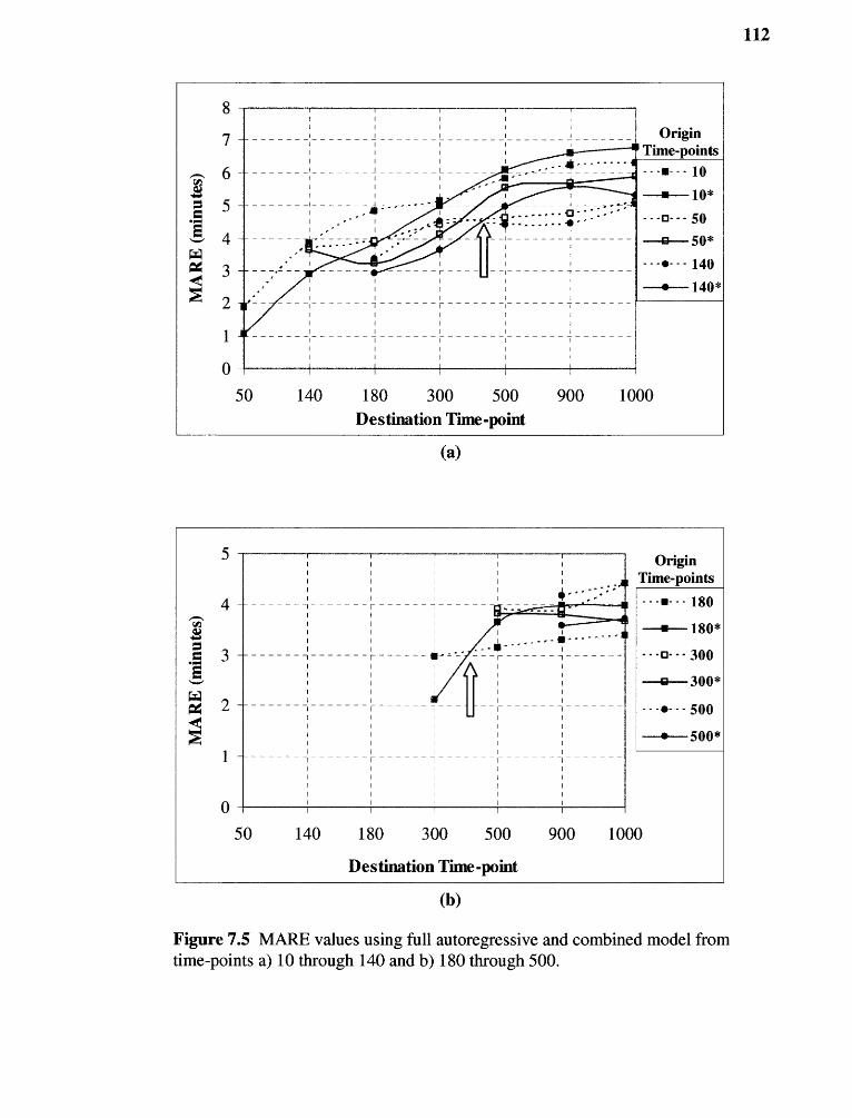
0
50 140 180 300 500 900 1000Destination Time-point
OriginTime-points
- - - w- - - 180
4,-- 180*
- - -a- - - 300
e--- 300*
- - -41- - - 500
—40-- 500*
50 140 180 300 500 900
1000
Destination Time -point
(a)
(b)
Figure 7.5 MARE values using full autoregressive and combined model fromtime-points a) 10 through 140 and b) 180 through 500.
112
113
In Figure 7.5, the MARE values obtained using the combined model and the full
autoregressive model only crossed each other between time-points TP=300 and TP=500,
when the prediction was performed from time-points TP=10 through 300. For example,
before the TP=300, the difference of MARE values using the combined model and full
autoregressive model for the curve corresponding to origin TP=10 is positive. This is
shown in Figure 7.5 by a block arrow. The difference of MARE values is negative after
TP=500. This observation indicates that the benefit of including delay propagation with
the autoregressive model to predict bus arrival times is not positive till TP=500.
This observation suggests the possibility of the existence of an optimal "location"
before which, the benefit of including delay propagation in the combined model may not
become beneficial in terms of a reduction in the arrival time prediction error. The reason
behind the positive benefits of including bus delay propagation with the full
autoregressive models after the "optimal location" is because of a significant portion of
the arrival time constitutes the predicted amount of delay , which is determined by the
Markov model.

CHAPTER 8
CONCLUSION
8.1 Results and Findings
In this research, bus arrival time prediction models were developed using historical bus
travel time information. The research used a stochastic approach to predict bus travel
time and delay propagation based on historical information of bus travel time and delay.
The existing bus travel and arrival time prediction models were studied to determine their
limitations. In this research, the appropriate stochastic time series models were
developed. The ability of the models to capture the temporal variations of bus travel time
was also determined. Since existing stochastic time series models do not consider the
propagation of bus delays to downstream stops, this research also focused on modeling
the propagation of delay of buses to downstream stops. The bus arrival time prediction
models were developed using a case study route and historical information on bus travel
times and delay were obtained.
The analysis of historical bus travel time showed that the coefficient of variation
differed between time-points. The coefficient of variation is consistently related to the
MAPE achieved using time series prediction models. Links with a higher coefficient of
variation had a higher MAPE and links with a lower coefficient of variation had a lower
MAPE. This is because of the presence of a larger proportion of a random component in
the observed travel time.
The recurring patterns of bus travel times were modeled by using full
autoregressive models, which produced better MAPE than other time series models. Full
114

115
autoregressive models also closely predicted bus travel times and were able to
accommodate variations in the observed travel time. The seasonal models and subset
autoregressive models failed to significantly improve the MAPE when compared with
full autoregressive models. Hence, only full autoregressive models were used to predict
bus travel times for links in the final analysis. The full autoregressive models also
performed better than historical average and smoothing models for all links in terms of
the MAPE for these models. Full autoregressive models showed a better fit than historical
average and smoothing models in terms of capturing the periodic variations during peak
periods.
The comparison of predicted and observed transition probabilities between delay
states results showed that the Markov process can adequately model the propagation of
delay to downstream stops using the assumption of heterogeneous delay propagation. The
chi-square comparisons between predicted and observed transition probabilities of links
did not follow the Markov process when using the assumption of homogeneous delay
propagation to downstream time-points.
The benefits of using bus delay propagation to predict bus arrival times at
downstream time-points were shown by producing a probability curve of the deviation
between predicted and observed arrival time. The normal curve of predicted delay is
narrower and less spread that the curve for observed delay. This showed the probability
of deviation from the scheduled arrival time is smaller if delay propagation is used to
predict bus arrival times. Hence, it is beneficial for transit agencies to relay predicted bus
arrival time to passengers by using only bus delay propagation at downstream stops than
not providing any information.

116
A separate analysis of the benefits associated with including the delay
propagation with the full autoregressive model to predict bus arrival times was also
performed. The positive benefits of delay propagation and its benefit to predict bus
arrival time at downstream stops were established. The inclusion of delay propagation
into the arrival time prediction algorithm decreased the relative error when predictions
were made at time-points with some distance from the origin time-point. These
conditions occurred because the contribution of the predicted bus delay at destination
time-points was significant in proportion to the predicted travel time. Finally, the
comparisons were made between results of the model using delay propagation only and
the combined model. In summary, the research results are as follows:
- The recurring patterns of bus travel times were modeled by using fullautoregressive models, which produced better MAPE than other time seriesmodels analyzed in the research.
- The comparison of predicted and observed transition probabilities betweendelay states showed that the Markov process can adequately model delaypropagation.
After analyzing the benefits of the bus arrival time prediction model using thepredicted delay only, it is beneficial to relay such arrival time information topassengers using the predicted delay only.
- A separate analysis of benefits from combining the delay propagation with thefull autoregressive models to predict bus arrival times was also performed.However, an optimal location exists along the route, after which the inclusionof delay propagation may not be beneficial.
- MARE values do not remain constant while predicting bus arrival time at atime-point. In this research, MARE values increased from 1 minute to 5minutes. The MARE values differed when predicting the bus arrival time at atime-point from two different upstream time-points.
117
8.2 Research Contributions
The objective of this research was to develop an arrival time prediction algorithm with
focus on bus operation conditions on urban streets. The case study used in this research
included suburban locations as well as downtown locations, so the research demonstrated
differences in the prediction algorithm between urban and suburban locations.
The methodology proposed in this research consisted of full autoregressive
models to predict bus travel times based on historical information and a Markov process
to predict delay at downstream time-points. The inclusion of bus delay propagation into
the bus arrival time prediction algorithm is an important contribution to the research
efforts to predict bus arrival times. A significant attempt has been made in this research to
explain the delay propagation phenomena into the arrival time prediction algorithm. It
was shown that the proposed methodology was able to produce significant benefits to
accurately predict bus arrival time by including delay propagation.
The research showed that the transit agencies can provide more accurate bus
arrival times by using delay propagation and a Markov process instead of using the
scheduled arrival time only to estimate the bus arrival time. Transit agencies can also
choose to use historical travel time information and predicted delay to provide more
accurate bus arrival time information.
The delay propagation model based on Markov chains is entirely based on
historical bus information. The model does not require collection of a large number of
variables. The literature review showed that bus arrival time prediction models were also
developed based on Kalman filters models using the current geographic location of the
bus and the predicted trajectory of the bus. However, this model requires a high polling

118
frequency to determine the geographic location of the bus. Another Kalman filter model
was based on historical bus travel time information and a constant headway of the bus.
This research, however, does not require frequent observation of the geographic location
of the bus and the assumption of constant headway is not made. The results of the
research showed that by using the historical information of delay propagation, bus arrival
time predictions can be done with accuracy of between 1 to 5 minutes for a total travel
time of 1.5 hours. Hence, by using delay propagation model based on Markov chains,
accurate bus arrival time predictions can be performed without collecting a large number
of bus operation variables, simulations and additional hardware requirements.
8.3 Recommendations for Future Research
In this research, the transition probabilities defining the delay states between the time-
points were determined based on heterogeneous conditions between time-points. Between
any two time-points, a constant transition probability matrix is used to define the
relationship between the delay states. However, the transition probabilities of delay states
between any two time-points can vary depending on temporal conditions. For example,
the transition probabilities may vary between peak and off-peak conditions and between
weekday and weekends for the same delay states. Hence, there is a possibility of more
accurately defining the transition probabilities between any two time-points based on
temporal variations. However, this requires a larger sample size than that used in this
research.
A larger sample size can obviously increase the accuracy of the transition
probabilities. However, the literature review showed that using a larger sample size

119
creates an opportunity to use more complex processes to obtain better estimates of the
transition probabilities, such as a Bayesian approach and non linear programming.
The research showed that there exists an optimal location. Before or after this
location, the inclusion of bus delay propagation into the arrival time prediction model
produces benefits or disbenefits. Hence, there is a possibility to determine a relationship
between the optimal location and the variables that influence bus arrival time, such as
distance from the origin, travel time, and number of time-points.

APPENDIX A
OBSERVED TRANSITION PROBABILITIES
The observed transition probabilities for each combination of time-points are provided in
the following tables.
Table A.1 Observed Transition Probabilities of Individual Links
Link jell P12 P13 P21 P22 P23 P31 P32 P33
10-50 0.876 0.119 0.005 0.107 0.893 0.000 0.000 0.500 0.500
50-140 0.922 0.026 0.052 0.353 0.647 0.000 0.000 0.000 1.000
140-180 0.777 0.215 0.008 0.050 0.900 0.050 0.667 0.000 0.333
180-300 0.865 0.125 0.010 0.146 0.854 0.000 0.200 0.200 0.600
300-500 0.790 0.189 0.021 0.132 0.868 0.000 0.250 0.000 0.750
500-900 0.898 0.020 0.082 0.105 0.895 0.000 0.000 0.500 0.500
900-1000 0.887 0.113 0.000 0.000 1.000 0.000 0.545 0.182 0.273
Table A.2 Observed Transition Probabilities of Links from TP=10
Link P11 P12 P13 P21 P22 P23 P31 P32 P33
10-140 0.905 0.048 0.048 0.595 0.380 0.025 0.500 0.000 0.500
10-180 0.653 0.327 0.02 0.622 0.378 0.000 0.000 0.000 0.000
10-300 0.762 0.201 0.037 0.596 0.385 0.019 0.333 0.000 0.667
10-500 0.715 0.252 0.033 0.436 0.526 0.038 0.333 0.333 0.333
10-900 0.657 0.224 0.119 0.383 0.553 0.064 0.000 0.000 0.000
10-1000 0.637 0.312 0.050 0.431 0.558 0.009 0.000 0.500 0.500
120

121
Table A.3 Observed Transition Probabilities of Links from TP=50
Link p11 P12 P13 P21 p22 P23 P31 P32 P33
50-180 0.591 0.386 0.023 0.222 0.778 0.000 0.000 0.000 1.000
50-300 0.770 0.194 0.036 0.256 0.744 0.000 0.111 0.000 0.889
50-500 0.714 0.241 0.045 0.227 0.773 0.000 0.500 0.333 0.167
50-900 0.607 0.262 0.131 0.300 0.700 0.000 0.500 0.500 0.000
50-1000 0.632 0.308 0.060 0.324 0.676 0.000 0.556 0.333 0.111
Table A.4 Observed Transition Probabilities of Links from TP=140
Link p11 P12 P13 P21 P22 p 23 P31 P32 P33
140-300 0.790 0.195 0.015 0.056 0.944 0.000 0.310 0.000 0.690
140-500 0.671 0.298 0.031 0.000 1.000 0.000 0.500 0.250 0.250
140-900 0.594 0.323 0.083 0.167 0.833 0.000 0.333 0.000 0.667
140-1000 0.607 0.353 0.040 0.118 0.882 0.000 0.621 0.276 0.103
Table A.5 Observed Transition Probabilities of Links from TP=180
Link pH P12 P13 P21 p 22 P23 P31 P32 P33
180-500 0.574 0.368 0.059 0.206 0.794 0.000 0.636 0.182 0.182
180-900 0.421 0.447 0.132 0.360 0.520 0.120 0.667 0.000 0.333
180-1000 0.562 0.371 0.067 0.179 0.795 0.026 0.750 0.188 0.063
Table A.6 Observed Transition Probabilities of Links from TP=300
Link pii P12 P13 P21 P22 P23 P31 P32 P33
300-900 0.711 0.171 0.118 0.171 0.800 0.029 0.250 0.250 0.500
300-1000 0.708 0.257 0.035 0.143 0.857 0.000 0.292 0.542 0.167

APPENDIX B
PREDICTED TRANSITION PROBABILITIES
The predicted transition probabilities for each combination of time-points are provided in
the following tables.
Table B.1 Predicted Transition Probabilities of Links from TP=10
Link P11 p12 P13 P21 P22 P23 P31 P32 P33
10-140 0.849 0.100 0.051 0.414 0.581 0.006 0.176 0.324 0.500
10-180 0.699 0.272 0.029 0.354 0.611 0.034 0.487 0.329 0.184
10-300 0.650 0.326 0.024 0.403 0.573 0.024 0.506 0.379 0.115
10-500 0.563 0.405 0.032 0.400 0.573 0.026 0.479 0.424 0.097
10-900 0.548 0.390 0.062 0.420 0.534 0.046 0.475 0.438 0.088
10-1000 0.520 0.463 0.017 0.397 0.590 0.013 0.469 0.507 0.024
Table B.2 Predicted Transition Probabilities of Links from TP=50
Link p11 P12 P13 P21 P22 p23 P31 P32 P33
50-180 0.752 0.222 0.026 0.307 0.658 0.035 0.667 0.000 0.333
50-300 0.689 0.288 0.023 0.369 0.607 0.024 0.644 0.150 0.206
50-500 0.588 0.380 0.032 0.378 0.597 0.026 0.580 0.252 0.168
50-900 0.568 0.368 0.064 0.402 0.554 0.044 0.547 0.321 0.132
50-1000 0.539 0.444 0.017 0.380 0.608 0.012 0.557 0.407 0.036
122
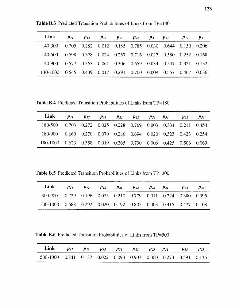
123
Table B.3 Predicted Transition Probabilities of Links from TP=140
Link P11 P12 P13 P21 P22 P23 P31 P32 P33
140-300 0.705 0.282 0.012 0.185 0.785 0.030 0.644 0.150 0.206
140-500 0.598 0.378 0.024 0.257 0.716 0.027 0.580 0.252 0.168
140-900 0.577 0.363 0.061 0.306 0.659 0.034 0.547 0.321 0.132
140-1000 0.545 0.439 0.017 0.291 0.700 0.009 0.557 0.407 0.036
Table B.4 Predicted Transition Probabilities of Links from TP=180
Link P11 p 12 P13 P21 P22 P23 P31 P32 P33
180-500 0.703 0.272 0.025 0.228 0.769 0.003 0.334 0.211 0.454
180-900 0.660 0.270 0.070 0.286 0.694 0.020 0.323 0.423 0.254
180-1000 0.623 0.358 0.019 0.265 0.730 0.006 0.425 0.506 0.069
Table B.5 Predicted Transition Probabilities of Links from TP=300
Link p11 P12 p 13 P21 p 22 p 23 P31 P32 P33
300-900 0.729 0.196 0.075 0.210 0.779 0.011 0.224 0.380 0.395
300-1000 0.688 0.292 0.020 0.192 0.805 0.003 0.415 0.477 0.108
Table B.6 Predicted Transition Probabilities of Links from TP=500
Link P11 P12 P13 P21 P22 P23 P31 P32 P33
500-1000 0.841 0.137 0.022 0.093 0.907 0.000 0.273 0.591 0.136

APPENDIX C
GRAPHICAL COMPARISONS OF TRANSITION PROBABILITIES
The graphical comparisons between observed and predicted transition probabilities at
different origin time-points are shown in the following figures.
124

520 900 1000180 300
Time-points Predicted - p 1 1 —a— Actual - p 11Predicted - p 12 Actual - p 12
—)k— Predicted - p 13 --a— Actual - p 13
1.00
0.80
en 0.60
R., 0.40
t:2.•
0.20
0.00 ok-140 180
Time-points
300 520 900 1000
Predicted Actual- p21
Predicted -p22
Predicted
--IF- - p21
-- Actual - p22
- p23 --a— Actual - p23
125
(a)
(b)
Figure C.1 Comparison of predicted and observed transition probabilities a) p 1./
and b)p2j assuming heterogeneous propagation of delay for TP=50.
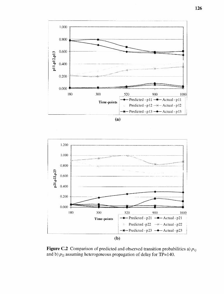
1.000
0.800
0.600
0.400
0.200
0.000
300
Time-points
520 900 1000
---4-- Predicted - p 21 —1— Actual - p21
Predicted -p 22 - Actual - p22
Predicted - p 23 —11-- Actual - p23
1.200
1.000
0.800
0.600
0.400
0.200
0.000
180
520 900 1000Predicted - p 11 —11— Actual - p 11Predicted - p 12 Actual - p 12
--*— Predicted - p 13 —1— Actual - p 13
180 300
Time -points
(a)
(b)
Figure C.2 Comparison of predicted and observed transition probabilities a) pand b) p2i assuming heterogeneous propagation of delay for TP=140.
126
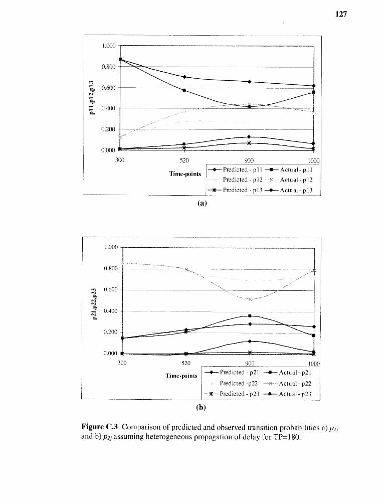
900 1000-4- Predicted - p21 -a- Actual - p21
Predicted -p22 -- Actual - p22
Predicted - p23 -8- Actual - p23
520
Time-points
1.000
0.800
N 0.600
C.-4 0.400CL
0.200
0.000
300
1.000
0.800
S, 0.600
7.1 0.400
0.200
0.000 300 520
Time-points
900
1000-4- Predicted - p 11 -a-- A ctu al - p 11
Predicted - p 12 Actual - p 12
Predicted - p13 Actual - p 13
(a)
(b)
Figure C.3 Comparison of predicted and observed transition probabilities a) p ij
and b) p2, assuming heterogeneous propagation of delay for TP=180.
127

520Time-points
1.000
0.800
S., 0.600
7-1 0.400CL
900 1000
Predicted - p 11 —is—Actual - p 11
Predicted - p 12 - Actual - p 12
Predicted - p 13 Actual - p 13
0.000
1 .000
0.800
520 900
—4-- Predicted - p 21
Predicted -p22
Predicted - p23
1 000
Time-points --a— Actual- p21
Actual - p22
--o— Actual - p23
(a)
(b)
Figure C.4 Comparison of predicted and observed transition probabilities a)and b) p2j assuming heterogeneous propagation of delay for TP=300.
128
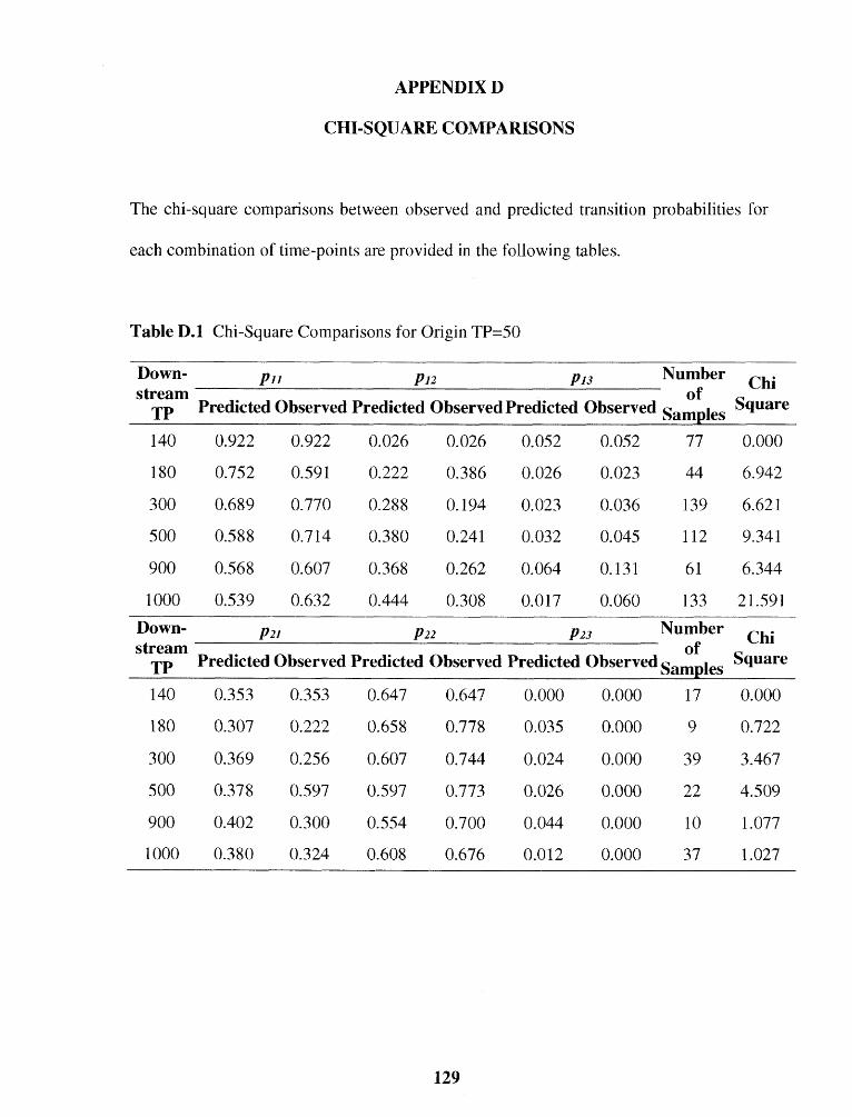
APPENDIX D
CHI-SQUARE COMPARISONS
The chi-square comparisons between observed and predicted transition probabilities for
each combination of time-points are provided in the following tables.
Table D.1 Chi-Square Comparisons for Origin TP=50
Down- P11 P12 P13 Number ChiSquarestream of
TP Predicted Observed Predicted Observed Predicted Observed Samples
140 0.922 0.922 0.026 0.026 0.052 0.052 77 0.000
180 0.752 0.591 0.222 0.386 0.026 0.023 44 6.942
300 0.689 0.770 0.288 0.194 0.023 0.036 139 6.621
500 0.588 0.714 0.380 0.241 0.032 0.045 112 9.341
900 0.568 0.607 0.368 0.262 0.064 0.131 61 6.344
1000 0.539 0.632 0.444 0.308 0.017 0.060 133 21.591Down- P21 P22 P23 Number Chi
Squarestream ofTP Predicted Observed Predicted Observed Predicted Observed Samples
140 0.353 0.353 0.647 0.647 0.000 0.000 17 0.000
180 0.307 0.222 0.658 0.778 0.035 0.000 9 0.722
300 0.369 0.256 0.607 0.744 0.024 0.000 39 3.467
500 0.378 0.597 0.597 0.773 0.026 0.000 22 4.509
900 0.402 0.300 0.554 0.700 0.044 0.000 10 1.077
1000 0.380 0.324 0.608 0.676 0.012 0.000 37 1.027
129

0.777 0.777 0.215 0.215 0.008 0.008
0.705 0.790 0.282 0.195 0.012 0.015
0.598 0.671 0.378 0.298 0.024 0.031
0.577 0.594 0.363 0.323 0.061 0.083
0.545 0.607 0.439 0.353 0.017 0.040
121 0.000
205 7.681
161 4.481
96 1.262
201 11.300
130
Table D.2 Chi-Square Comparisons for Origin TP=140
Down-Numberpii P12 p13 Chistream ofTP Predicted Observed Predicted Observed Predicted Observed Samples
Square
180
300
500
900
1000
Down- P21 P22 P23 Number Chistream ofTP Predicted Observed Predicted Observed Predicted Observed Samples
Square
180 0.050 0.050 0.900 0.900 0.050 0.050 20 0.000
300 0.185 0.056 0.785 0.944 0.030 0.000 36 5.530
500 0.257 0.000 0.716 1.000 0.027 0.000 21 8.336
900 0.306 0.167 0.659 0.833 0.034 0.000 12 1.731
1000 0.291 0.118 0.700 0.882 0.009 0.000 34 5.435
Table D.3 Chi-Square Comparisons for Origin TP=180
Down-NumberpH P12 P13 Chistream ofTP Predicted Observed Predicted Observed Predicted Observed Samples
Square
300 0.865 0.865 0.125 0.125 0.010 0.010 104 0.000
500 0.703 0.574 0.272 0.368 0.025 0.059 68 6.910
900 0.660 0.421 0.270 0.447 0.070 0.132 38 9.742
1000 0.623 0.562 0.358 0.371 0.019 0.067 89 11.458Down- P21 P22 P23 Number Chistream ofTP Predicted Observed Predicted Observed Predicted Observed Samples
Square
300 0.146 0.146 0.854 0.854 0.000 0.000 41 0.000
500 0.228 0.206 0.769 0.794 0.003 0.000 34 0.209
900 0.286 0.360 0.694 0.520 0.020 0.120 25 13.913
1000 0.265 0.179 0.730 0.795 0.006 0.026 39 4.170

131
Table D.4 Chi-Square Comparisons for Origin TP=300
Down- P11 P12 P13 Number Chistream ofTP Predicted Observed Predicted Observed Predicted Observed Samples
Square
500 0.790 0.790 0.189 0.189 0.021 0.021 143 0.000
900 0.729 0.711 0.196 0.171 0.075 0.118 76 2.182
1000 0.688 0.708 0.292 0.257 0.020 0.035 171 2.573
Down-NumberP21 P22 P23 Chistream ofTP Predicted Observed Predicted Observed Predicted Observed Samples
Square
500 0.132 0.132 0.868 0.868 0.000 0.000 53 0.000
900 0.210 0.171 0.779 0.800 0.011 0.029 35 1.294
1000 0.192 0.143 0.805 0.857 0.003 0.000 70 1.328
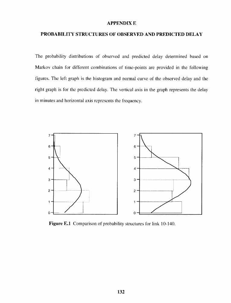
APPENDIX E
PROBABILITY STRUCTURES OF OBSERVED AND PREDICTED DELAY
The probability distributions of observed and predicted delay determined based on
Markov chain for different combinations of time-points are provided in the following
figures. The left graph is the histogram and normal curve of the observed delay and the
right graph is for the predicted delay. The vertical axis in the graph represents the delay
in minutes and horizontal axis represents the frequency.
Figure E.1 Comparison of probability structures for link 10-140.
132
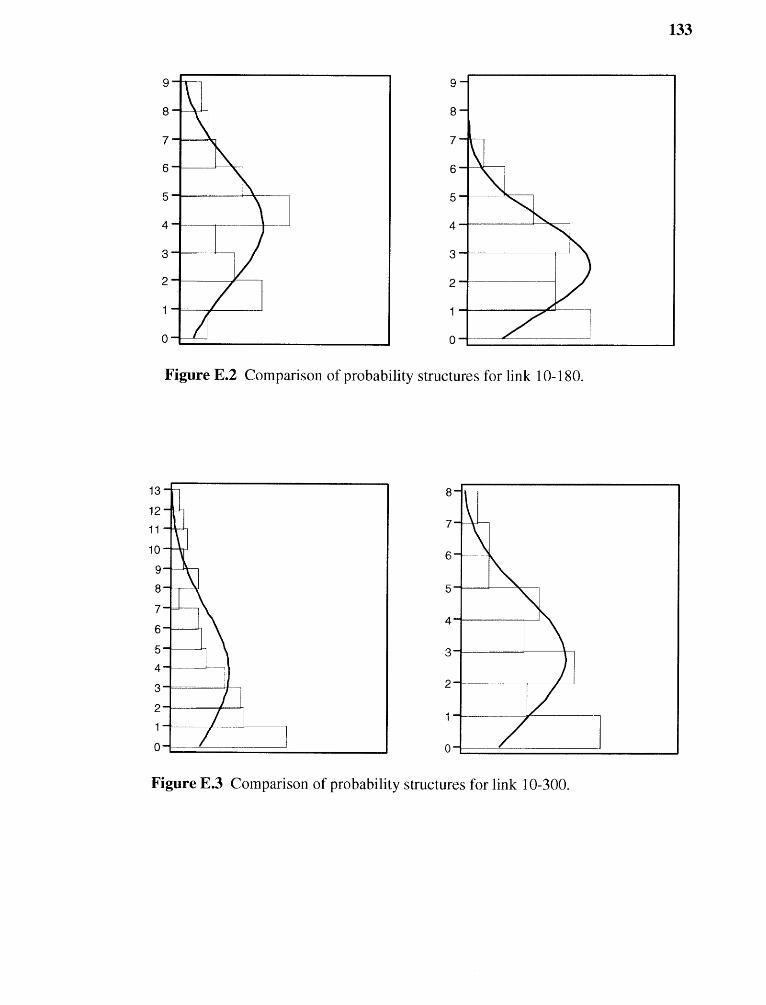
7-
6-
5
4 -
3 -
2-
1-
0 -
133
Figure E.2 Comparison of probability structures for link 10-180.
Figure E.3 Comparison of probability structures for link 10-300.

134
1 5
1 0
5 ....._
6 -
4
3 -
2
1 -
0 -
Figure E.4 Comparison of probability structures for link 10-500.
1 0
9
8 -
-7
6
5
4
3
2
1 --
0
1 0 -
9 -
8
7
6
5
4-
3
2 -
1 -
0—
Figure E.5 Comparison of probability structures for link 10-900.
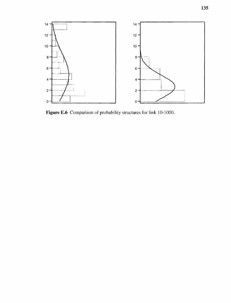
14
12
10 -
8 -
6 •••••■■---
4 -
2
0—
135
14-
12 -
10 -
Figure E.6 Comparison of probability structures for link 10-1000.

REFERENCES
Abdelfattah, A. M., and Khan, A. M., Models for Predicting Bus Delays, TransportationResearch Record 1623, Transportation Research Board, 1998.
Ahmed, M. S., and Cook, A. R., Analysis of Freeway Traffic Time-Series Data by UsingBox-Jenkins Techniques, Transportation Research Record 722, TransportationResearch Board, 1979.
Al-Deek, H. M., D'Angelo, M. P., Wang, M. C., Hendrickson, C. T., and Ritchie, S. G.,Travel Time Prediction with Non-Linear Time Series, Fifth InternationalConference on Applications of Advanced Technologies in TransportationEngineering, 1998.
Anderson, T. W, and Goodman, L. A., Statistical Inference about Markov Chains, TheAnnals of Mathematical Statistics, Volume 28, Number 1, pp. 89-110, 1957.
Arem, B. V., Kirby, H. R., Vlist, M. J., and Whittaker, J. C., Recent Advances andApplications in the Field of Short-Term Traffic Forecasting, International Journalof Forecasting, Volume 13, pp. 1-12, 1997.
Bae, S., and Kachroo, P., Proactive Travel Time Predictions under Interrupted FlowConditions, Vehicle Navigation and Information Systems ConferenceProceedings, Seattle, Washington, IEEE, pp. 179-186, 1995.
Bowerman, B., and O'Connell, R., Time Series Forecasting: Unified Concepts andComputer Implementation, Second Edition, Duxbury Press, Boston, 1987
Box, G. E. P., and Jenkins, G. M., Time Series Analysis: Forecasting and Control,Holden-Day, San Francisco, California, 1970.
Brockwell, P. J., and Davis, R. A., Introduction to Time Series and Forecasting, SecondEdition, Springer-Verlag New York Inc., 2002.
Bus Arrival and Departure Study, Translink Research Center, Texas TransportationInstitute, 2000.
Chatfield, C., Time-series Forecasting, Chapman & Hall/CRC, 2000.
Chatfield, C., The Analysis of Time Series: An Introduction, Chapman & Hall, 1984.
Chien, I. J., and Kuchipudi, C. M., Dynamic Travel Time Prediction with Real-time andHistorical Data, Transportation Research Board, Washington D.C., 2002.
Dailey, D. J., and Cathey, F. W., Transit Vehicles as Traffic Probe Sensors,Transportation Research Board, 81 st Annual Meeting, Washington D.C., 2002.
136
137
Dailey, D. J., Wall, Z. R., Maclean, S. D., and Cathey, F. W., An Algorithm andImplementation to Predict the Arrival of Transit Vehicles, IntelligentTransportation Systems Conference Proceedings, Michigan, IEEE, pp. 161-166,2000.
Ding, Y., and Chien, I. J., Dynamic Bus Arrival Time Prediction with Artificial NeuralNetworks, Journal of Transportation Engineering, Volume 128, Issue 5, pp. 429-438, 2002.
Dion, F., and Rakha, H., Estimating Spatial Travel Times using Automatic VehicleIdentification Data, Transportation Research Board, 82' Annual Meeting,Washington D.C., 2003.
Dixon, M. P., and Rilett, L. R., Real Time Origin-Destination Estimation usingAutomatic Vehicle Identification Data, Transportation Research Board, 79 thAnnual Meeting, Washington D.C., 2000.
Eisele, W. L., AVL Systems for Bus Transit, TCRP Synthesis 24, Transit CooperativeResearch Program, Transportation Research Board, National Research Council,1997.
Evans, J. L., Elefteriadou, L., Gautam, N., Probability of breakdown at freeway mergesusing Markov chains, Transportation Research Part B, Volume 35, pp 237-254,2001.
Franco, G., and Taranto, C. D., Public Transit Vehicle Journey Time PredictionTechniques: Approach and Developments in the Context of Torino Prompt TestSite, Proceedings of the First World Congress on Advanced Transport Telemnaticsand Intelligent Vehicle Highway Systems, ERTICO, pp. 2848-2855, 1995.
Frechette, L. A., and Khan, A. M., Bayesian Regression-Based Urban Traffic Models,Transportation Research Record 1644, Transportation Research Board, 1998.
Fuller, W. A., Introduction to Statistical Time Series, John Wiley & Sons, 1976.
Guidance for Developing and Deploying Real-Time Information Systems for Transit,Federal Transit Administration, U.S. Department of Transportation, WashingtonD.C., 2003.
Hamed, M. M., Al-Masaeid, H. R., and Bani Said, Z. M., Short-Term Prediction ofTraffic Volume in Urban Arterials, Journal of Transportation EngineeringVolume 121, Number 3, 1995.
Horbury, A. X., Using Non Real-Time Automatic Vehicle Location Data to Improve BusServices, Transportation Research Part B, Volume 33, pp. 559-570, 1999.

138
Hounsell, N., MeLeod, F., and Ishtiaq, S., Journey Time Prediction for Bus Priority atTraffic Signals, Transportation Systems Conference, International Federation onAutomatic Control, Volume 2, pp. 871-876, 1997.
Hu, K., and Wong, C.K., "Deploying Real-Time Bus Arrival Information and TransitManagement Systems in Los Angeles", Proceedings of the ITS America 12 th
Annual Meeting, California, 2002.
Ishak, S., and Al-Deek, H., Performance Evaluation of Short-Term Time-Series TrafficPrediction Model, Journal of Transportation Engineering, Volume 128, No. 6, pp.490-498, 2002.
Kemeny, J.G. and Snell, J.L, Finite Markov Chains, Springer-Verlag, 1976.
Lee, S., and Fambro, D. B., Application of Subset Autoregressive Integrated MovingAverage Model for Short-Term Freeway Traffic Volume Forecasting,Transportation Research Record 1678, Transportation Research Board, 1998.
Lee, T.C., Judge, G. G., and Zellner, A., Maximum Likelihood and Bayesian Estimationof Transition Probabilities, Journal of American Statistical Association, Volume63, Number 324, pp. 1162-1179, 1968.
Lin, W. H. and Bertini, R. L., Modeling Schedule Recovery Processes in TransitOperations for Bus Arrival Time Prediction, Intelligent Transportation SystemsProceedings, IEEE, 2002.
Lin, W., Kuikarni, A., Mirchandani, P., Arterial Travel Time Estimation for AdvancedTraveler Information Systems, Transportation Research Board, 82nd AnnualMeeting, Washington D.C., 2003.
Lin, W., and Zeng, J., An Experimental Study on Real-Time Bus Arrival Time Predictionwith GPS Data, Transportation Research Record 1667, Transportation ResearchBoard, 1999.
Lindveld, Ch. D. R., Thijis, R., Bovy, P. H. L., and Van der Zijpp, N. J., Evaluation ofOn-line Travel Time Estimators and Predictors, Transportation Research Record1719, Transportation Research Board, 2000.
Makridakis, S., and Wheelwright, S. C., Forecasting Methods and Applications, JohnWiley & Sons, 1978.
Maybeck, P. S., Stochastic Models, Estimation and Control, Volume I, Academy Press,New York, 1979.
Naus, J. I., Data Quality Control and Editing, Marcel Dekker, Inc., New York, 1975.

139
Park, D., Rilett, L. R., and Han, G., Spectral Basis Neural Networks for Real-Time TravelTime Forecasting, Journal of Transportation Engineering, pp. 515-523, 1995.
Patnaik, J., Chien, S., Bladikas, A., Estimation of Bus Arrival Times using APC Data,Journal of Public Transportation, Volume 7, Number 1, 2004.
Real-Time Bus Arrival Information Systems-A Synthesis of Transit Practices, TCRP 48,Transit Cooperative Research Program, Transportation Research Board, 2003.
Robertson, C., A Matrix Regression Model for the Transition Probabilities in a FiniteState Stochastic Process, Applied Statistics, Volume 39, Number 1, pp. 1-19,1990.
Ross, P., Exponential Filtering of Traffic Data, Transportation Research Record 869,Transportation Research Board, 1982.
Shalaby, A., and Farhan, A., Bus Travel Time Prediction Model for Dynamic OperationsControl and Passenger Information Systems, Transportation Research Board,82 nd Annual Meeting, Washington D.C., 2003.
Shalaby, A., Lyon, C., and Sayed, T., Transferability of Travel Time Models andProvision of Real-Time Arrival Time Information, IEEE IntelligentTransportation Systems Conference Proceedings, California, 2001
Smith, B. L., Williams, B. M., and Oswald, R. K., Comparison of Parametric andNonparametric Models for Traffic Flow Forecasting, Transportation ResearchPart C, Volume 10, Issue 4, pp. 303-321, 2002.
Stathopoulos, A., and Karlaftis, M., Temporal and Spatial Variations of Real-TimeTraffic Data in Urban Areas, Transportation Research Board, 82nd AnnualMeeting, Washington D.C., 2003.
Strathman, J.G., Kimpel, T.J., Dueker, K.J., Gerhart, R.L., Turner, K., Griffin, D., andCallas, S., Bus Transit Operation Control: Review and an Experiment InvolvingTri-Met's Automated Bus Dispatching System, Journal of Public Transportation,Volume 4, Number 1, pp. 1-26, 2001.
Taylor, H. M., and Karlin, S., An Introduction to Stochastic Modeling, 3 rd Edition,Academic Press, 1998.
Turner, S. M., Guidelines for Developing ITS Data Archiving Systems, Report 2127-3,Texas Transportation Institute, 2001.
Turner, S. M., ITS Data Archiving: Case Study Analysis of San Antonio TRANSGUIDEData, Report FHWA-PL-99-024, Texas Transportation Institute, 1999.

140
Vining, G. G., Statistical Methods for Engineering, Duxbury Press, 1998.
Welch, G., and Bishop, G., An Introduction to the Kalman Filter, University of NorthCarolina at Chapel Hill, ACM Inc., 2001.
William, B. M., Durvasula, P. K., and Brown, D. E., Urban Freeway Traffic FlowPrediction: Application of Seasonal Autoregressive Integrated Moving Averageand Exponential Smoothing Models, Transportation Research Record 1644,Transportation Research Board, 1998.