copyright warning & restrictionsarchives.njit.edu/vol01/etd/1990s/1997/njit-etd1997-021/...ld l...
TRANSCRIPT

Copyright Warning & Restrictions
The copyright law of the United States (Title 17, United States Code) governs the making of photocopies or other
reproductions of copyrighted material.
Under certain conditions specified in the law, libraries and archives are authorized to furnish a photocopy or other
reproduction. One of these specified conditions is that the photocopy or reproduction is not to be “used for any
purpose other than private study, scholarship, or research.” If a, user makes a request for, or later uses, a photocopy or reproduction for purposes in excess of “fair use” that user
may be liable for copyright infringement,
This institution reserves the right to refuse to accept a copying order if, in its judgment, fulfillment of the order
would involve violation of copyright law.
Please Note: The author retains the copyright while the New Jersey Institute of Technology reserves the right to
distribute this thesis or dissertation
Printing note: If you do not wish to print this page, then select “Pages from: first page # to: last page #” on the print dialog screen

The Van Houten library has removed some of the personal information and all signatures from the approval page and biographical sketches of theses and dissertations in order to protect the identity of NJIT graduates and faculty.

ABSTRACT
DISTRIBUTION OF VELOCITIES AND VELOCITY GRADIENTSIN MIXING AND FLOCCULATION VESSELS:
COMPARISON BETWEEN LDV DATA AND CFD PREDICTIONS
byChanggen Luo
Flocculation is an operation of significant industrial relevance commonly encountered in
many processes, including water and wastewater treatment. The physicochemical
phenomena of this process is strongly affected by the magnitude of the velocity gradients
generated, typically through agitation, in rapid mix devices and flocculation vessels.
In this work the fluid dynamic characteristics of mechanically agitated systems,
namely three different types of stirred tanks, which can be used as flocculation vessels,
were studied. Both the mean and fluctuating velocities in all three directions were
measured by using a Laser-Doppler Velocimeter (LDV). The velocity distribution,
fluctuating velocities, power consumption and local velocity gradient were numerically
predicted with FLUENT, a computational fluid dynamic (CFD) software, using k-s
model, algebraic stress model (ASM), or Reynolds Stress Model (RSM) to simulate
turbulence effect. The experimentally obtained mean velocities and turbulent kinetic
energies on the top and bottom horizontal surfaces of the region swept by the impeller
were used as boundary conditions in the simulations.
Significant agreement between the experimental data and the numerical
predictions of the three dimensional velocities and turbulent kinetic energies was
obtained in all cases.

A novel approach to numerically calculate the local velocity gradient (G) in
turbulent flocculation tanks was developed. The distribution of local G values in three
mixing systems was mapped through two new methods: the complete definition of local
velocity gradient method and the local energy dissipation method. Results show that
both methods can provide similar information about the local G value distribution. The
trajectory of a solid particle with physical properties similar to those to a floc particle
moving in three different mixing systems was numerically determined. The G value
experienced by the particle as a function of time was also determined. A new parameter,
the velocity gradient-time integral along a particle trajectory, was proposed and
calculated. It is expected that the approach developed in this study will provide the
foundations for a more accurate characterization of the fluid dynamics of flocculation
systems.

DISTRIBUTION OF VELOCITIES AND VELOCITY GRADIENTSIN MIXING AND FLOCCULATION VESSELS:
COMPARISON BETWEEN LDV DATA AND CFD PREDICTIONS
byChanggen Luo
A DissertationSubmitted to the Faculty of
New Jersey Institute of Technologyin Partial Fulfillment of the Requirements for the Degree of
Doctor of Philosophy
Department of Chemical Engineering,Chemistry, and Environmental Science
May 1997

Copyright ©1997 by Changgen Luo
ALL RIGHTS RESERVED

APPROVAL PAGE
DISTRIBUTION OF VELOCITIES AND VELOCITY GRADIENTSIN MIXING AND FLOCCULATION VESSELS:
COMPARISON BETWEEN LDV DATA AND CFD PREDICTIONS
Changgen Luo
Dr. Piero M. Armenante, Dissertation Advisor DateProfessor of Chemical Engineering, Chemistry, and Environmental Science, NJIT
Dr. GRton Lewandowski, Committee Member DateProfessor of Chemical Engineering, Chemistry, and Environmental Science, NJIT
Dr. Ching-Rong Huang, Committel-Member DateProfessor of Chemical Engineering, Chemistry, and Environmental Science, NJIT
Dr. Ernest S. Geskin, Committee Member DateProfessor of Mechanical Engineering, NJIT
Dr. Robert G. Luo, Comm' ee ember DateAssistant Professor of Ch al Engineering, Chemistry, and Environmental Science,NJIT

BIOGRAPHICAL SKETCH
Author: Changgen Luo
Degree: Doctor of Philosophy in Chemical Engineering
Date: May 1997
Undergraduate and Graduate Education:
• Doctor of Philosophy in Chemical EngineeringNew Jersey Institute of Technology, New Jersey, 1997
• Master of Science in Chemical EngineeringEast China University of Chemical Technology, Shanghai, P. R. China, 1988
• Bachelor of Science in Chemical EngineeringEast China University of Chemical Technology, Shanghai, P. R. China, 1985
Major: Chemical Engineering
Publications:
Armenante P. M., Luo C., Chou C. C., Fort I. and Medek J., "Velocity Profiles in aClosed, Unbaffled Vessel: Comparison between Experimental LDV Data andNumerical CFD Predictions", Chemical Engineering Science, in press, 1997.
iv

This dissertation is dedicated tomy wife and my daughter
ACKNOWLEDGMENT
I would like to take this opportunity to thank Dr. Piero M. Armenante for his
help and guidance. Without his support, this work would not have been done.
I would also like to express my sincere thanks to Dr. Gordon A. Lewandowski,
Dr. Ching-Rong Huang, Dr. Ernest S. Geskin and Dr. Robert G. Luo for serving as
Committee Members.
Special thanks go to Dr. Chun-Chiao Chou, Dr. Ding-Wei Zhou and Dr. Gong-
Wei Wang, Dr. Socrates Ioannidis. Their knowledge, wisdom, time, and effort have
made invaluable contributions to the conduct of the research and the completion of this
work. More importantly their friendship has made my time at NM an enjoyable
experience.
This work was partially supported by the National Science Foundation (Grant
Number EEC 9520573), whose contribution is gratefully acknowledged.
I would like to give special credit to many specialists from both TSI Inc. and
Fluent Inc. for their technical support in LDV experiment and CFD program usage.
Appreciation goes to our co-investigators from the Czech Republic and
Queen's University, Northern Ireland, for the information they provided and exchanged
with me.
Finally, I would like to express my deep appreciation to my wife for her
patience and considerate support.
vi
TABLE OF CONTENTS
Chapter Page
1 INTRODUCTION 1
2 OBJECTIVES 5
3 THEORETICAL BACKGROUND 6
3.1 Flocculation Process 6
3.1.1 Chemical Hydrolysis 6
3.1.2 Destabilization and Aggregation of Colloidal Particles 7
3.1.3 Fluid Dynamics Effects 8
3.2 Effect of Velocity Gradients on Flocculation 9
3.2.1 Conventional Method to Estimate the Velocity Gradient 9
3.2.2 Rigorous Methods to Calculate the Velocity Gradient 13
3.3 New Parameter for Flocculation Process 20
4 EXPERIMENTAL APPARATUS AND METHOD 22
4.1 Mixing and Flocculation Systems 22
4.2 LDV Systems 25
4.3 Experimental Determination of Velocity Distribution 27
4.4 Power Number 27
5 NUMERICAL SIMULATION 28
5.1 Computational Fluid Dynamic Models 28
5.1.1 k-6' Model 29
5.1.2 Algebraic Stress Model (ASM) 31
vii

TABLE OF CONTENTS(Continued)
Chapter Page
5.1.3 Reynolds Stress Model (RSM) 31
5.2 Boundary Conditions 32
5.3 Grid Generation 33
5.4 Power Consumption and Pumping Capacity 34
5.5 Local G Value Calculation 35
5.6 Particle Trajectory 36
5.7 G Value Distribution Along the Particle Trajectory 38
5.8 Velocity Gradient-Time Integral 39
6 RESULTS AND DISCUSSION 40
6.1 System A 40
6.1.1 LDV Measurements in the Impeller Region 40
6.1.2 Comparison between LDV Measurements and CFD Predictions 42
6.1.3 Comparison between Different Agitation Speeds 45
6.2 System B 47
6.2.1 LDV Measurements in the Impeller Region 48
6.2.2 Comparison between LDV Measurements and CFD Predictions 50
6.2.3 Velocity Gradient Distribution 52
6.2.4 Particle Trajectory 54
6.2.5 Velocity Gradient-Time Integral along the Particle Trajectory 55
viii
TABLE OF CONTENTS(Continued)
Chapter Page
6.3 System Cl 58
6.3.1 LDV Measurements in the Impeller Region 60
6.3.2 Comparison between LDV Measurements and CFD Predictions 61
6.3.3 Velocity Gradient Distribution 63
6.3.4 Particle Trajectory . 64
6.3.5 Velocity Gradient-Time Integral along the Particle Trajectory 65
6.4 System C2 67
6.4.1 LDV Measurements in the Impeller Region 68
6.4.2 Numerical Predicted Velocity Distribution 69
6.4.3 Velocity Gradient Distribution 70
6.4.4 Particle Trajectory .70
6.4.5 Velocity Gradient-Time Integral along the Particle Trajectory 71
6.5 Future Work 73
7 CONCLUSIONS 75
APPENDIX A. FIGURES FOR SYSTEM CONFIGURATIONS AND RESULTS 79
APPENDIX B. PROGRAM FOR THE LOCAL G VALUE CALCULATION 147
APPENDIX C. PROGRAM FOR THE NEW PARAMETER CALCULATION 154
REFERENCES 173
ix

LIST OF TABLES
Table Page
6-1 Comparison of Power Number and Flow Numbers for the UnbaffiedCylindrical Tank among Experimental Measurements and CFD Predictions 46
6-2 Comparison of G Average Value Between Two Methods 59

LIST OF FIGURES
Figure Page
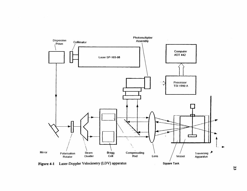
4-1 Laser-Doppler Velocimetry (LDV) apparatus 23
4-2 Configuration of unbaffted cylindrical mixing tank (System A) 80
4-3 Configuration of baffled rectangular mixing tank (System B) 81
4-4 Configuration of baffled rectangular mixing tank (System Cl and C2) 82
4-5 Outline of impellers: (a) 6-blade pitched bladed impeller, (b) 2-blade paddletype impeller 83
4-6 Measurement methods used in determining three velocity components 84
6-1 Experimentally determined (via LDV) dimensionless velocities and turbulentkinetic energies in the impeller region (System A, N = 450 rpm): (a)velocities at the top plane of the volume swept by the impeller; (b) velocitiesat the bottom plane of the volume swept by the impeller; (c) turbulentkinetic energies at the same two planes. positive values indicate upwardvelocities in the axial direction, or outward velocities in the radial direction. .... 85
6-2 Grid used in the CFD simulation for System A (2D view) 86
6-3 Grid used in the CFD simulation for System A (3D view) 87
6-4 Comparison between experimental tangential velocity measurements (viaLDV) and numerical predictions (via CFD) at five horizontal locations(WI) using asm and k-e turbulence models (System A, N = 450 rpm) 88
6-5 Comparison between experimental axial velocity measurements andnumerical predictions (System A, N = 450 rpm) 89
6-6 Comparison between experimental radial velocity measurements andnumerical predictions (System A, N = 450 rpm) 90
6-7 Comparison between experimental and numerically predicted turbulentkinetic energies (System A, N = 450 rpm) 91
6-8 CFD prediction of velocity distribution in System A (N = 450 rpm) (a):tridimensional view; (b) cross sectional view across the shaft 92
xi

LIST OF FIGURES(Continued)
Figure Page
6-9 Experimentally determined (via LDV) dimensionless velocities and turbulentkinetic energies in the impeller region (System A, N = 700 rpm): (a)velocities at the top plane of the volume swept by the impeller; (b) velocitiesat the bottom plane of the volume swept by the impeller; (c) turbulentkinetic energies at the same two planes. positive values indicate upwardvelocities in the axial direction, or outward velocities in the radial direction 93
6-10 Comparison between experimental tangential velocity measurements (viaLDV) and numerical predictions (via CFD) at five horizontal locations(Z/H) using ASM and k-e turbulence models (System A, N = 700 rpm) 94
6-11 Comparison between experimental axial velocity measurements andnumerical predictions (System A, N = 700 rpm) 95
6-12 Comparison between experimental radial velocity measurements andnumerical predictions (System A, N = 700 rpm) 96
6-13 Comparison between experimental and numerically predicted turbulentkinetic energies (System A, N = 700 rpm) 97
6-14 Experimentally determined (via LDV) dimensionless velocities and turbulentkinetic energies in the impeller region (System B, N = 350 rpm): (a)velocities at the top plane of the volume swept by the impeller; (b) velocitiesat the bottom plane of the volume swept by the impeller; (c) turbulentkinetic energies at the same two planes. positive values indicate upwardvelocities in the axial direction, or outward velocities in the radial direction 98
6-15 Grid used in the CFD simulation in System B (2D view) 99
6-16 Grid used in the CFD simulation in System B (3D view) 100
6-17 Comparison between LDV measurements and CFD predictions: tangentialvelocity in System B (N = 350 rpm) 101
6-18 Comparison between LDV measurements and CFD predictions: axialvelocity in System B (N = 350 rpm) 102
6-19 Comparison between LDV measurements and CFD predictions: radialvelocity in System B (N = 350 rpm) 103
xii
LIST OF FIGURES(Continued)
Figure Page
6-20 Comparison between LDV measurements and CFD predictions: turbulentkinetic energy in System B (N = 350 rpm) 104
6-21 CFD prediction of velocity distribution in System B using RSM (2D view) 105
6-22 CED prediction of velocity distribution in System B using RSM (3D view) 106
6-23 CFD prediction of velocity distribution in System B using RSM (top view:Z/H = 0.18) 107
6-24 CFD prediction of velocity distribution in System B using RSM (top view:Z/H = 0.37) 108
6-25 CFD prediction of velocity distribution in System B using RSM (top view:Z/H = 0.70) 109
6-26 CFD prediction of velocity gradient distribution in System B (by completedefinition of local velocity gradient, curve labels give the value of logioG) 110
6-27 CFD prediction of velocity gradient distribution in System B (by localenergy dissipation method, curve labels give the value of log ioG) 111
6-28 CFD prediction of particle trajectory in System B (t = 2,000 s) 112
6-29 CFD prediction of particle trajectory in System B (t = 10,000 s) 113
6-30 G value along the particle trajectory in System B 114
6-31 G value distribution curve along the particle trajectory in System B 115
6-32 Cumulative G value distribution along the particle trajectory in System B 116
6-33 Numerical integration of (t * G) vs. time (along the particle trajectory) inSystem B 117
6-34 Average G value vs. time (along the particle trajectory) in System B 118
6-35 Experimentally determined (via LDV) dimensionless velocities and turbulentkinetic energies in the impeller region (System Cl, N = 159 rpm) 119
6-36 Grid used in the CFD simulation for System Cl (2D View) 120
xiii

LIST OF FIGURES(Continued)
Figure Page
6-37 Grid used in the CFD simulation for System C1 (3D View) 121
6-38 Comparison between LDV measurements and CFD predictions: tangentialvelocity (System Cl, N = 159 rpm) 122
6-39 Comparison between LDV measurements and CFD predictions: axialvelocity (System Cl, N = 159 rpm) 123
6-40 Comparison between LDV measurements and CFD predictions: radialvelocity (System Cl, N = 159 rpm) 124
6-41 Comparison between LDV measurements and CFD predictions: turbulentkinetic energy (System Cl, N = 159 rpm) 125
6-42 CFD prediction of velocity distribution in System C1 (2D View) 126
6-43 CFD prediction of velocity distribution in system Cl (3D View) 127
6-44 CFD prediction of velocity gradient distribution in System Cl (curve labelsgive the value of log1oG , where G is in s-1) 128
6-45 CFD prediction of particle trajectory in System Cl (t = 2,000 s) 129
6-46 CFD prediction of particle trajectory in System Cl (t = 10,000 s) 130
6-47 G value along the particle trajectory in system C1 131
6-48 G value distribution curve along the particle trajectory in system Cl 132
6-49 Cumulative G value distribution along the particle trajectory in System Cl 133
6-50 Numerical integration of (t * G) vs. time (along the particle trajectory) in
System Cl 134
6-51 Average G value vs. time (along the particle trajectory) in System Cl 135
6-52 Experimentally determined (via LDV) dimensionless velocities and turbulentkinetic energies in the impeller region (System C2, N= 256 rpm) 136
6-53 CFD prediction of velocity distribution in System C2 (2D view) 137
xiv
LIST OF FIGURES(Continued)
Figure Page
6-54 CFD prediction of velocity distribution in System C2 (3D view) 138
6-55 CFD prediction of velocity gradient distribution in System C2 (curve labelsgive the value of logioG , where G is in s4) 139
6-56 CFD prediction of particle trajectory in System C2 (t = 2,000 s) 140
6-57 CFD prediction of particle trajectory in System C2 (t = 10,000 s) 141
6-58 G value along the particle trajectory in System C2 142
6-59 G value distribution curve along the particle trajectory in System C2 143
6-60 Cumulative G value distribution along the particle trajectory in System C2 144
6-61 Numerical integration of (t * G) vs. time (along the Particle Trajectory) inSystem C2 145
6-62 Average G value vs. time (along the particle trajectory) in System C2 146
xv

NOMENCLATURE
Cp C2, C3, C4, C5, CD, C, Constants used in the CFD simulation; dimensionless
d Particle diameter in flocculation process; m
D Impeller diameter; m
Fl Impeller flow number (Q/ND3); dimensionless
G Velocity gradient; s4
Gave Average velocity gradient within the entire vessel; s -1
Gk Generation of turbulence kinetic energy, k; kg/m•s3
H Height of liquid in mixing vessel; m
k Turbulent kinetic energy; 2m is2
m Mass of liquid in vessel; kg
n Particle concentration in flocculation process; dimensionless
no Initial particle concentration in flocculation process; dimensionless
N Agitation speed; rotations/s
Np Power number; dimensionless
P Power dissipation; W
Pave Average power dissipation for the entire vessel; W
Q, Qu, Q, Variables used in CFD simulation (ASM model); m 2/s3
Q, Impeller discharge flow rate; m3 /s
r Radial distance from vessel centerline; m
R Radius of impeller; m
t Time; s
xvi

NOMENCLATURE(Continued)
T Vessel diameter; m
u Velocity; m/s
u Velocity vector; rn/s
ii Time averaged velocity vector; m/s
u' Fluctuating velocity vector; m/s
ua Axial (vertical) velocity; rn/s
lir Radial velocity; m/s
ut Tangential velocity; m/s
uy ', u,' Fluctuating velocity in three directions, respectively; m/s
Utu, Impeller tip velocity; m/s
w Vertically projected width of impeller blade; m
xi , xi, x1 Coordinate variables; m
Z Axial (vertical) distance from vessel bottom; m
Zb Axial (vertical) distance from vessel bottom to bottom of impeller region; m
Z4- Axial (vertical) distance from vessel bottom up to the point on the impeller tip
where the radial flow on the impeller side is directed outwards; m
Greek Letters
a Constant used during the numerical simulation of turbulence (equation 2);
dimensionless
xvii

\ T = Power numberp N3D5
NOMENCLATURE(Continued)
Kronecker delta
e Turbulence energy dissipation rate; m 2/s3
Save Average turbulence energy dissipation rate within the entire vessel; m 2/s3
ri Collision efficiency in flocculation process; dimensionless
,u. Turbulent viscosity; kg/(m•s)
,u Liquid viscosity; kg/(m•s)
v Kinematic viscosity; m2.s-1
p Liquid density; kg/m3
al, Constant used in the CFD simulation; dimensionless
Constant used in the CFD simulation; dimensionless
r Torque at shaft; N•m
Q Volume fraction of colloidal particles in flocculation process; dimensionless
Dimensionless Groups:
N./3 2 pRe Impeller Reynolds number
xvi i i
CHAPTER 1
INTRODUCTION
Mechanically agitated mixing vessels are widely used in a variety of industrial
applications, such as precipitation, flocculation, polymerization, fermentation, as well as
crystallization and heterogeneous catalysis. As a result, a significant literature exists on
the subject, and design principles have been determined for many situations of industrial
significance. In recent years the flow distribution in agitated vessels has been studied
primarily using two complementary techniques, Laser-Doppler Velocimetry (LDV) and
Computational Fluid Dynamics (CFD) simulations. Computational fluid dynamics (CED)
is a tool that is becoming increasing popular to study complex fluid flows such as those
typically found in mixing vessels. The main advantage of this approach is in its potential
for reducing the extent and number of experiments required to describe such types of
flow. These two tools have enabled investigators to experimentally and non-intrusively
determine the velocity distribution in mixing vessels, and make quantitative predictions
about the same velocities (Armenante and Chou, 1996; Bakker, 1992; Costes et al.,
1991; De Groot, 1991; Dong, 1994; Hirata et al., 1991; Jaworski et al., 1991; Kresta and
Wood, 1991; Mahouast et al., 1989; Weetman, 1991; Ranade et al., 1989, 1992)
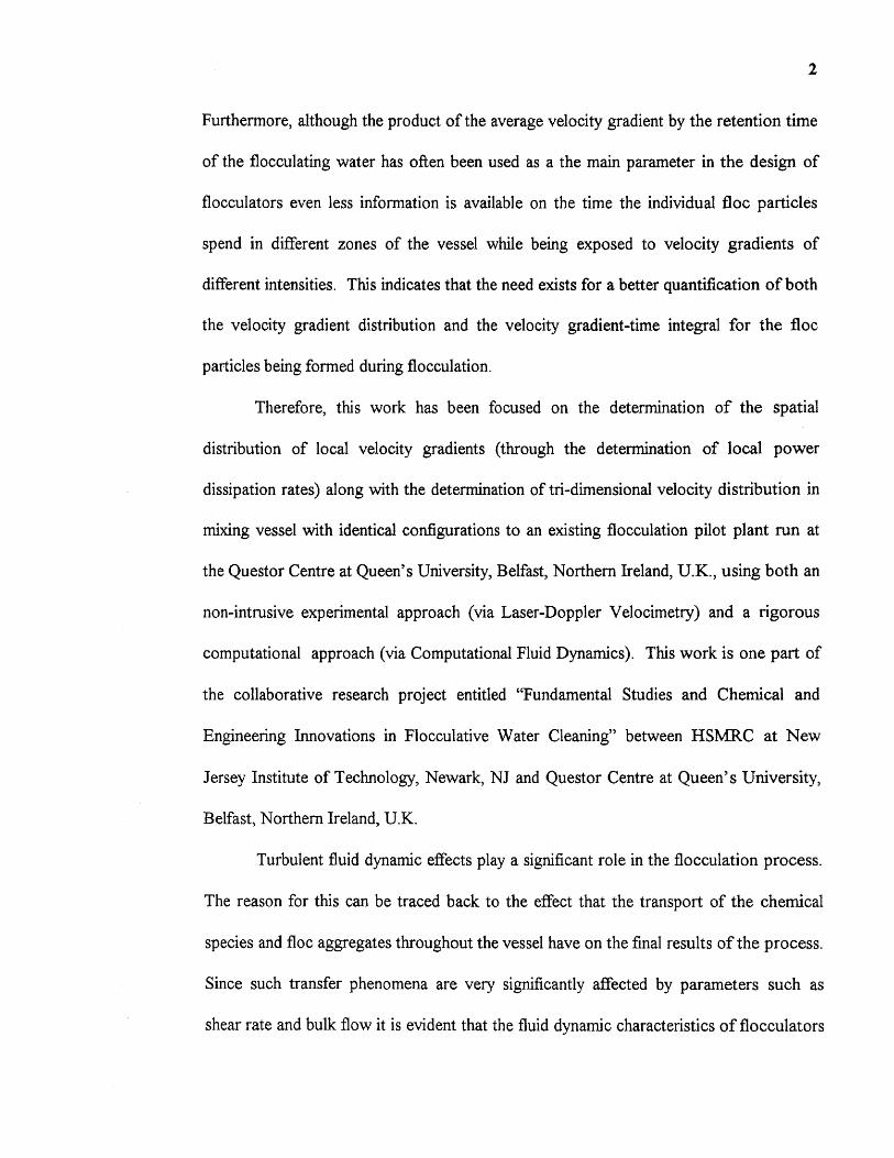
Some industrial processes, such as flocculation, are strongly affected by the
magnitude of the velocity gradients generated, typically through agitation. However,
only rough estimates of such velocity gradients (based on the average power dissipation
in the flocculation vessel) are currently available. Very little information is available
from the literature on the distribution of velocity gradients throughout the flocculation
vessel (especially the fluctuating velocity gradients produced by turbulence effects).
1
2
Furthermore, although the product of the average velocity gradient by the retention time
of the flocculating water has often been used as a the main parameter in the design of
flocculators even less information is available on the time the individual floc particles
spend in different zones of the vessel while being exposed to velocity gradients of
different intensities. This indicates that the need exists for a better quantification of both
the velocity gradient distribution and the velocity gradient-time integral for the floc
particles being formed during flocculation.
Therefore, this work has been focused on the determination of the spatial
distribution of local velocity gradients (through the determination of local power
dissipation rates) along with the determination of tridimensional velocity distribution in
mixing vessel with identical configurations to an existing flocculation pilot plant run at
the Questor Centre at Queen's University, Belfast, Northern Ireland, U.K., using both an
non-intrusive experimental approach (via Laser-Doppler Velocimetry) and a rigorous
computational approach (via Computational Fluid Dynamics). This work is one part of
the collaborative research project entitled "Fundamental Studies and Chemical and
Engineering Innovations in Flocculative Water Cleaning" between HSMRC at New
Jersey Institute of Technology, Newark, NJ and Questor Centre at Queen's University,
Belfast, Northern Ireland, U.K.
Turbulent fluid dynamic effects play a significant role in the flocculation process.
The reason for this can be traced back to the effect that the transport of the chemical
species and floc aggregates throughout the vessel have on the final results of the process.
Since such transfer phenomena are very significantly affected by parameters such as
shear rate and bulk flow it is evident that the fluid dynamic characteristics of flocculators

3
are of paramount importance for both an understanding of the process and its actual
practical results. This is a very well recognized aspect of flocculation known to any
practitioner in the field. In fact, the most common flocculation test, the jar test, is an
attempt to capture the essence of both the fluid dynamic characteristics and the particle
destabilization and floc aggregation aspects of the process. Unfortunately, this approach
is very crude and results it produces are difficult to extrapolate.
The main difficulty at the basis of a precise definition of the fluid dynamic
characteristics of flocculators is that flocculation is dominated by turbulence, a
phenomenon still poorly understood. In recent years the study of turbulent phenomena
has been greatly been enhanced by experimental tools such as Laser-Doppler
Velocimetry. In addition, fluid dynamic problems have been successfully tackled by
numerically solving the equations commonly used to described turbulent phenomena.
This work is aimed at utilizing these tools to quantitatively describe the fluid dynamics of
flocculators.
In this study the velocities in four mixing and flocculation systems (System A: an
unbaified, flat-bottom, cylindrical vessel provided with a lid, completely filled with
water, and agitated by a six-blade, 45° pitched-blade turbine; System B: a baffled
rectangular tank agitated by a 2-blade paddle-type impeller; System Cl and C2: baffled,
flat-bottomed cylindrical vessels agitated by six-blade, 45° pitched-blade turbines of
different sizes) were experimentally determined with a laser-Doppler velocimetry (LDV)
apparatus. The velocities at a number of locations in the impeller region (defined as the
outer surface of the volume swept by the impeller) were then used as boundary
conditions in CFD simulations. The velocity distribution, fluctuating velocities, power

4
consumption and local velocity gradient were numerically predicted with FLUENT, a
computational fluid dynamic (CFD) software, using k-s model, algebraic stress model
(ASM), or Reynolds Stress Model (RSM) to simulate turbulence effect. Comparisons
were made between the experimental LDV data obtained for all three systems and the
results of the numerical predictions, in order to determine the best approach to CFD
simulation of complex flows in mixing and flocculation vessels.
In addition, a novel approach to numerically calculate the local velocity gradient
(G) in turbulent flocculation tanks was developed. The distribution of local G values in
two mixing systems was mapped through two new methods: the complete definition of
local velocity gradient method and the local energy dissipation method. Results show
that both methods can provide similar information about the local G value distribution.
The trajectory of a solid particle with physical properties similar to those to a floc
particle moving in three different mixing systems was numerically determined. The G
value experienced by the particle as a function of time was also determined.
In order to better characterize the effect of fluid dynamics on the flocculation
process, a new parameter, the velocity gradient-time integral, was proposed in this work.
A rigorous program to quantify this new parameter from the information obtained by
CFD simulation has been developed in this work by using Visual Basic language
incorporated with Microsoft Excel 5.0. Finally, a comparison was made between the G
average value obtained through the conventional method and the new method in this
work.
CHAPTER 2
OBJECTIVES
The primary objective of this work was the determination of the spatial distribution of
local velocity gradients (through the rigorous methods proposed in this work, i.e., the
complete definition of local velocity gradient method and the local energy dissipation
rate method) and the determination of tridimensional velocity distribution in four
mixing/flocculation systems. The trajectory of a virtual particle with physical properties
similar to those of a floc particle moving in three different systems was also numerically
determined. Both an non-intrusive experimental approach (via Laser-Doppler
Velocimetry) and a rigorous computational approach (via Computational Fluid
Dynamics) were used to achieve these objectives.
A new variable, the velocity gradient-time integral along a particle trajectory,
taking into account the local velocity gradient and the time a moving floc particle is
exposed to it, was then defined and calculated for three different systems to better model
the flocculation process. It is expected that the results of this approach will eventually
be incorporated in some of the many models available in the literature for floc
aggregation and breakage. So far these models have typically relied on averages of the
velocity gradient derived from simplified turbulence theories rather than their actual
values.
5
CHAPTER 3
THEORETICAL BACKGROUND
3.1 Flocculation Process
Flocculation process is an operation of significant industrial relevance commonly
encountered in water and wastewater treatment plants. Coagulation and flocculation
refer, respectively, to the process of destabilization of colloidal particles upon the
addition of some chemicals to the water containing them, and to the process through
which these destabilized particles collide and aggregate to form larger floc particles that
can be separated via sedimentation or other physical methods. The two terms are often
used interchangeably - a practice that will also be followed in this work, unless leading to
possible misunderstanding. Flocculation is a process extremely difficult to quantify
because of the complexities of the phenomena at its origin, and also because these
phenomena affect each other in ways that are difficult to resolve into separate effects.
When a coagulant is added to a solution containing colloidal particles a number
of aspects must be considered to fully explain the overall results. Chemical hydrolysis,
particle agglomeration and breakup, and turbulent fluid dynamic effects all play a
significant role in the overall process (Amirtharajah and Mills, 1982). These
characteristics of flocculation processes will now be briefly reviewed.
3.1.1 Chemical Hydrolysis
Most of the chemicals commonly used as coagulants react with water forming hydrolysis
products. In many cases the number and nature of these products are such that complex
equilibria among such species is possible. Furthermore, the composition of the resulting
6

7
solution is a strong function of pH and temperature. For example, the addition of ferric
chloride to water results in its hydrolysis to Fe(OH) 3 which then results in the formation
of species such as Fe(OH)4, Fe(OH)2+, Fe(OH)2+, Fe3+ and others. Equilibrium diagram
for all the species involved have been produced and are quite complex. An additional
complication results from the fact that the kinetics of the formation of the various
products during coagulation must be taken into account, and that only some of these
species are effective as coagulants.
3.1.2 Destabilization and Aggregation of Colloidal Particles
After its initial formation the coagulation products are typically adsorbed on the surface
of the colloid particles, destabilizing them. This is usually a fast reaction. However, in
order for the destabilized particles to aggregate they must come in contact with each
other and be maintained in such close proximity for a sufficient period of time for the
floc to be formed. Successive floc growth occurs when floc particles come in contact
with other particles, producing flocculation. This is typically a slower process. The two
aspects of the process have resulted in the common practice of carrying out flocculation
first under rapid mix conditions (where interactions among destabilized particles are
promoted) and then under slow mix conditions (where floc breakup is minimized and
sedimentation is promoted).
8
3.1.3 Fluid Dynamics Effects
The two previous aspects of the coagulation/flocculation process can be significantly
affected by the fluid dynamic conditions inside the flocculation vessel. The reason for
this can be traced back to the effect that the transport of the chemical species and floc
aggregates throughout the vessel have on the final results of the process. Since such
transfer phenomena are very significantly affected by parameters such as shear rate and
bulk flow it is evident that the fluid dynamic characteristics of flocculators are of
paramount importance for both an understanding of the process and its actual practical
results. This is a very well recognized aspect of flocculation known to any practitioner in
the field. The common alternation of "rapid mix" and "slow mix" regimes during
flocculation is a recognition that agitation is indeed a key parameter. In fact, the most
common flocculation test, the jar test, is an attempt to capture the essence of both the
fluid dynamic characteristics and the particle destabilization and floc aggregation aspects
of the process. Unfortunately, this approach is very crude and results it produces are
difficult to extrapolate.
The main difficulty at the basis of a precise definition of the fluid dynamic
characteristics of flocculators is that flocculation is dominated by turbulence, a
phenomenon still poorly understood. In recent years the study of turbulent phenomena
has been greatly enhanced by experimental tools such as laser-Doppler Velocimetry
(LDV). In addition, fluid dynamic problems have been successfully tackled by
numerically solving the equations commonly used to describe turbulent phenomena.
This work is aimed at utilizing these tools to quantitatively describe the fluid dynamics of
ao2
ai a & a(a, 8141 2
-+- -+-
9
flocculators so that it can be eventually incorporated in more comprehensive chemical-
physical flocculation models.
3.2 Effect of Velocity Gradients on Flocculation
Flocculation process is strongly affected by the magnitude of the velocity gradients
generated, typically, through agitation. In flocculation the velocity gradient is important
not only because it can produce contact between particles, but also because it can
produce floc breakup if it has too high a value.
3.2.1 Conventional Method to Estimate the Velocity Gradient
Because of the complexity of the flocculation process a number of simplified models as
well as rules of thumb are available from the literature (Bhargava and Ojha, 1993;
Delichatsios and Probstein, 1975; Dharmappa et al., 1993; Glasgow and Kim, 1986;
Glasgow and Liu, 1991; Mhaisalkar et al., 1991; Wiesner, 1992). In the vast majority of
these models the effect of agitation and turbulence on flocculation is typically expressed
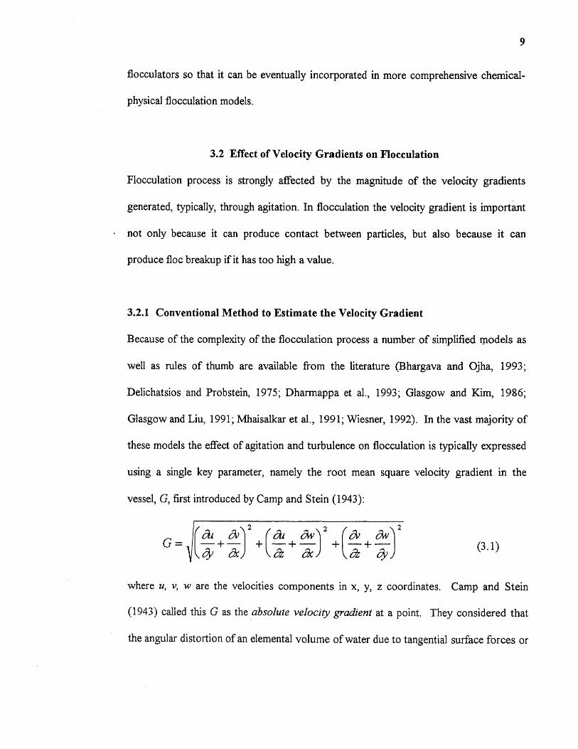
using a single key parameter, namely the root mean square velocity gradient in the
vessel, G, first introduced by Camp and Stein (1943):
G = (3.1)
where u, v, w are the velocities components in x, y, z coordinates. Camp and Stein
(1943) called this G as the absolute velocity gradient at a point. They considered that
the angular distortion of an elemental volume of water due to tangential surface forces or

G P= —
1, (3.3)
10
shears. Therefore, they related this absolute velocity gradient with the work done per
unit volume per unit time in the following way.
P2= jiG
where P = power dissipation, V = vessel volume, = liquid viscosity.
Rearranging Eq. 3.2, they had
(3.2)
where e= dissipation rate, v= kinematic viscosity.
Theoretically, if the power dissipated or the work done at any point within
agitated vessel is known, then the absolute velocity gradient can be calculated by using
the above equation. However, realistically, the dissipated power varies from position to
position within the agitated vessel. Therefore, the velocity gradient in this expression is a
function of both time and position within the vessel. Since the velocity gradients are
quite difficult to calculate, an approximation typically made to estimate G is to replace it
with its average value throughout the vessel Gay, :
P aveG = (3.4)
where the average power consumption, Pave, can easily be obtained from the power
requirement to agitate the vessel:
Pave = Np p .N3 D5 (3.5)

11
with Np = power number for a given impeller, p = density of liquid, N = rotational speed
of impeller, D = impeller diameter.
Gave obtained through equation 3.4 is referred to in this work as the G average
value obtained through the conventional method.
Gave or another mean value for G is typically included in most flocculation
models. For example, O'Melia (1972) assumed that the rate of change in the total
concentration of particles during flocculation is:
do _ 2rid 3 n 2=
dt 3
where n = particle concentration, ri = collision efficiency, d = particle diameter. Upon
integration this equation becomes:
in— =n 411Q G taveno 7C
where no = initial particle concentration, SZ = volume fraction of colloidal particles, and t
= time. A similar approach was also followed by Miyanami et al. (1982) who obtained
an expression in which ln(n/n o) was proportional to Goy,1.11. Other recommendations for
optimum flocculation include a number of different relationships in which the term Gave a
tfi can be found (Camp, 1955; McConnachie, 1989).
It is evident that the use of Gave instead of G greatly simplifies the calculation of
the frequency collision and hence the determination of the optimal flocculation
conditions. Unfortunately, in stirred tanks used in flocculation the distribution of
velocity gradients is by no means uniform. In fact, it has been shown already that the
(3.6)
(3.7)

12
local power consumption at location of high turbulence intensity (e.g., in the vicinity of
the impeller) can be many times higher than that in the rest of the tank (Wu and
Patterson, 1989; Kresta and Wood, 1991; Tatterson, 1991; Geisler et al, 1996)).
Furthermore, different mixing devices can produce identical average power dissipation
values (and hence identical Gave values) but very different distributions of e and G
throughout the vessel. As stated by Zhou and Kresta (1996): "Different types of
impellers create different circulation patterns and different distributions of turbulence
energy dissipation for the same tank geometry. The same average power input per unit
mass (sometimes called the average energy dissipation) can result in widely different
distributions of turbulence energy dissipation when different impellers are used with the
same tank geometry". Ducoste et al (1997) also pointed that: "There is growing
evidence that a more complex relationship exists between particle agglomeration/breakup
and the fluid mechanics generated in a flocculation basin that can not be fully described
by just using the G value for the whole tank. In order to fully understand the relationship
between agglomeration/breakup and fluid mechanics, it is necessary to first characterize
the complex fluid mechanics." °
Furthermore, the time a floc particle exposed to a given velocity gradient during
the flocculation processing is also very important. A particle may spend more time in
zones with one G value than other zones with different G value. This will make big
difference for certain flocculation process. A closer examination reveals that what can be
of ever greater significance for these two phenomena is a parameter that takes into
account not only the local velocity gradient but also the time a particle or floc is exposed

13
to it. The simplest conceivable function that includes both parameters is the product
Gave t„t in which ire, is the retention time. In fact, this group appears in the flocculation
equation by O'Melia given above. However, it is evident that even in the simple O'Melia
model the cumulative change in flocculation at a generic time will depend on the integral
of G as a function of time. Since during the same time interval the particle or floc has
followed a certain trajectory within the vessel the integral of G vs. t must be calculated
knowing what the trajectory is and the velocity that the particle has at each point.
Therefore, the term Gave tret obtained through the conventional method is only a crude
estimation of the actual velocity gradient-time integral.
3.2.2 Rigorous Methods to Calculate the Velocity Gradient
Although the conventional method to estimate the velocity gradient, proposed by Camp
and Stein (1943), has been widely used by environmental engineers for decades, it is a
very rough method. Apparently, it has two major weaknesses, at least. First, the so-
called absolute velocity gradient is defined in such a way that only the tangential shear
stresses were considered, while the normal stress terms were not included. This leads to
an incomplete estimation of this parameter. Second, an average velocity gradient is
calculated for the entire agitated vessel. This leads to a very inaccurate estimation of this
parameter, since the velocity gradient varies greatly from position to position within the
vessel. A simple value cannot represent the characteristics of this process. Besides,
different agitated systems could have the same Gave but produce quite different mixing or
flocculating results.

14
Because of these weaknesses, many researchers have found that Gave is not
suitable to describe the turbulent flocculation process. Argaman and Kaufman (1970)
experimentally observed that the maximum floc size in flocculation process was inversely
proportional to G. Cleasby (1984) even proposed that power input per unit mass to the
two thirds power, 1, is a more appropriate flocculation parameter than G obtained by
the conventional method for common water and wastewater flocculation practice. All
attempts available in the literature are based on the use of an average parameter for the
entire vessel, which can be inadequate to characterize the turbulent flocculation process.
No information was found in the literature about the estimation of local velocity gradient
in mixing or flocculation processes.
This work aimed to solve this problem. With the assistance of new technologies
in both experimental and simulation fields (LDV and CFD, respectively), we were able to
calculate the real value of this parameter (local velocity gradient) at each position within
the mixing or flocculation vessel, through more fundamental and rigorous methods
shown below.
A differential mechanical energy balance for a fluid element can be written as
(Bird et al. 1960):
O2 pv 2 - (V • pV 2 - (V • p v) (V •[rc • v Da
(3.8)+ p(v • g) p(—V • v) (—T:V v)
where the term on the left hand side is the rate of increase in kinetic energy per unit
volume, and the terms on the right hand side are the net rate of input of kinetic energy by
virtue of bulk flow, the rate of work done by pressure of surroundings on volume
=V (3.9)
2 ( city) 2 ± az) 2
4:13sv = 2■ 4) a
2 : 61,0 2 +( a z) 2
( » 61)
a4-2-1 2 + +alz)2c)
a.3 a 6)a ly atz1 2
L
= {2
15
element, the rate of work done by viscous force on volume element, the rate of work
done by gravity force on volume element, the rate of reversible conversion to internal
energy, and the rate of irreversible conversion to internal energy, respectively.
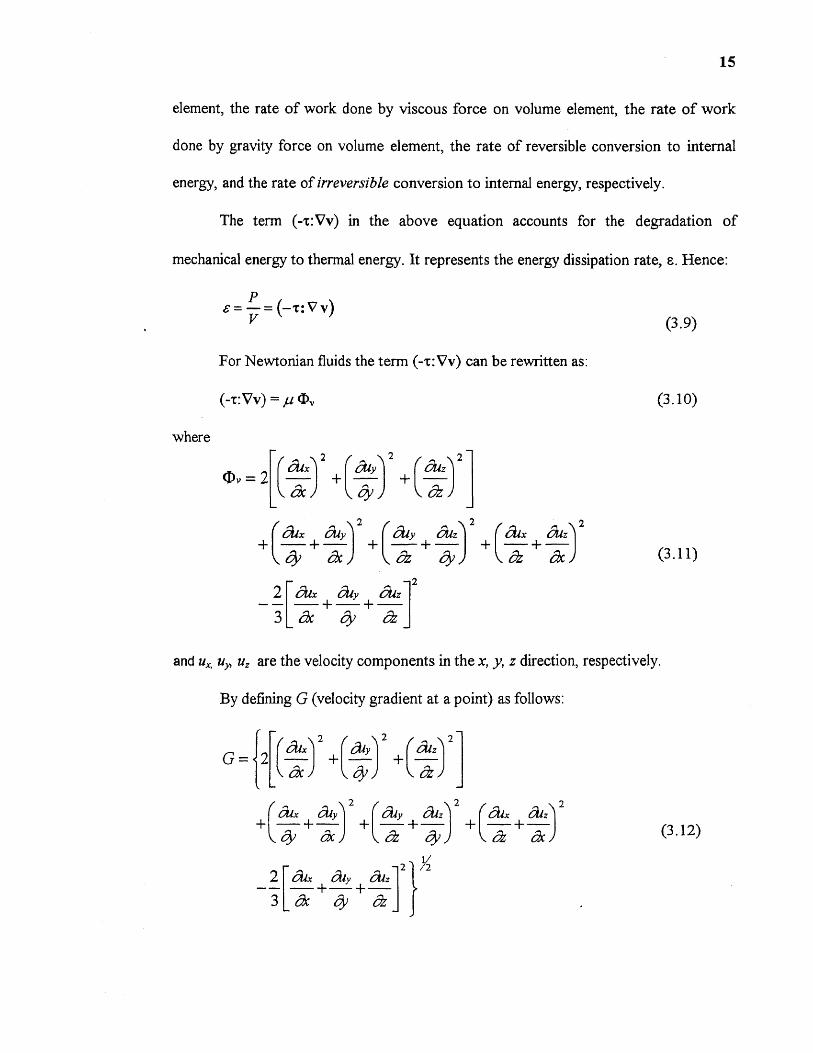
The term (-t: Vv) in the above equation accounts for the degradation of
mechanical energy to thermal energy. It represents the energy dissipation rate, E. Hence:
For Newtonian fluids the term (-t: Vv) can be rewritten as:
(-t: Vv) = iu
where
(3.10)
aix Oily) 2 (ado 5u+
Le3) 76-c) L-01 +-47
aix .4_ za ) 2
a a)2 ratc+cio+Ouz
2
6) a
and ux, uy, u, are the velocity components in the x, y, z direction, respectively.
By defining G (velocity gradient at a point) as follows:
(3.12)
(3.11)
(3.14)
G= {22 +r -ia,10 + 1,0)
dr I r c19 raz)UL
16
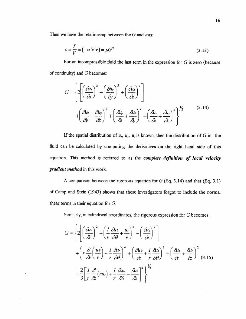
Then we have the relationship between the G and e as:
E- P
=(—T:Vv)=pG 2 (3.13)V
For an incompressible fluid the last term in the expression for G is zero (because
of continuity) and G becomes:
ay) 2 (az 2
••■•■•
G= {2
2 .\ 2aix ay) +ray + +(aix +azoy c oz 6) ) a a
If the spatial distribution of ux, uy, uz is known, then the distribution of G in the
fluid can be calculated by computing the derivatives on the right hand side of this
equation. This method is referred to as the complete definition of local velocity
gradient method in this work.
A comparison between the rigorous equation for G (Eq. 3.14) and that (Eq. 3.1)
of Camp and Stein (1943) shows that these investigators forgot to include the normal
shear terms in their equation for G.
Similarly, in cylindrical coordinates, the rigorous expression for G becomes:
2 + late azy + raiz + alr)2
Li' r) re%) a r oO c a (3.15)
2 10 1 aio air—3 r clz (rui-)+ +r
z- = duds (3.17)
17
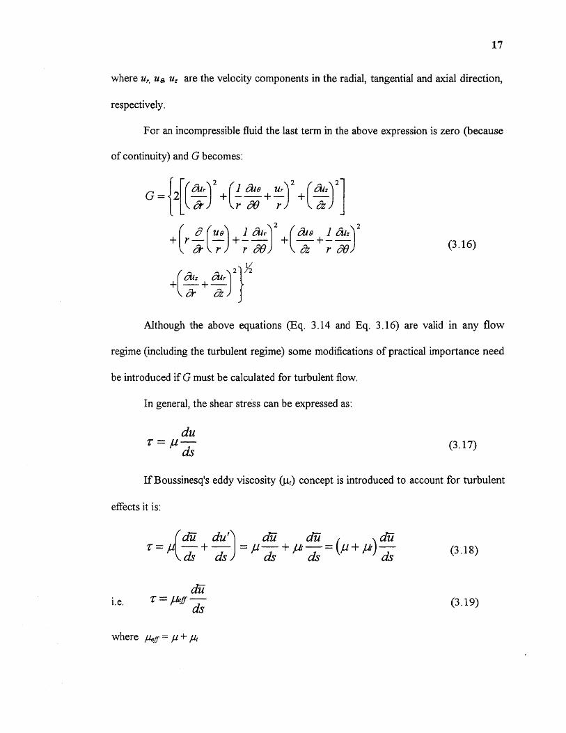
where ur, u Q u, are the velocity components in the radial, tangential and axial direction,
respectively.
For an incompressible fluid the last term in the above expression is zero (because
of continuity) and G becomes:
2 2 2
G — 12 ( +(10+1&) +(2)
r r
2 2
( 12!r) 71 clid Or) ( 6:9+ -1r aig )11
(3.16)
Although the above equations (Eq. 3.14 and Eq. 3.16) are valid in any flow
regime (including the turbulent regime) some modifications of practical importance need
be introduced if G must be calculated for turbulent flow.
In general, the shear stress can be expressed as:
If Boussinesq's eddy viscosity (p) concept is introduced to account for turbulent
effects it is:
"du du' &Ccz• = p p = .4_ pi)ds
(3.18)ds ds ds ds
i.e. I- = (3.19)
where "Jeff = + ,ut
du peff
ds(3.20)
Cax oily 2 (1Xy a-2\2+(-+ - -,acw,c a-z)
OIL O )
(3.21)
a.a.r ) 2 + (.;:1 4:90 + Err ) 2
+ azcl) 2
2( r—e9 (Flo) cl-r) ± r a-z) 2
r r 9 09z r (3.22)
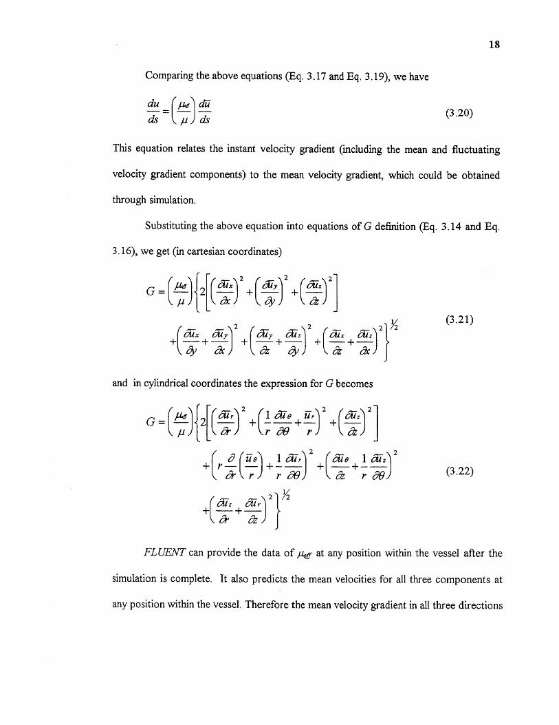
Comparing the above equations (Eq. 3.17 and Eq. 3.19), we have
18
This equation relates the instant velocity gradient (including the mean and fluctuating
velocity gradient components) to the mean velocity gradient, which could be obtained
through simulation.
Substituting the above equation into equations of G definition (Eq. 3.14 and Eq.
3.16), we get (in cartesian coordinates)
G =( 1-1-1 -ff)r GR,c)2 + I + ia) )
and in cylindrical coordinates the expression for G becomes
; tXr)
a. a
FLUENT can provide the data of j.i at any position within the vessel after the
simulation is complete. It also predicts the mean velocities for all three components at
any position within the vessel. Therefore the mean velocity gradient in all three directions
G = (3.24)
19
for any position within the vessel can be calculated. Thus we were able to calculate the
local velocity gradient at any position within the agitated vessel.
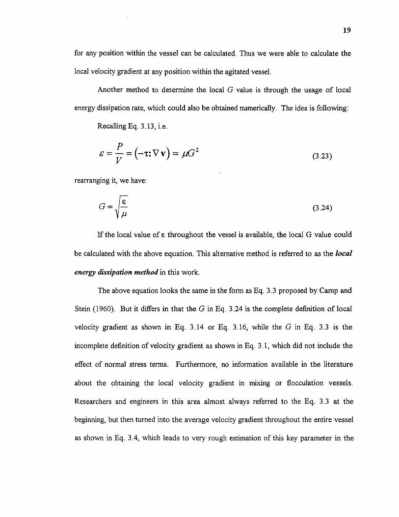
Another method to determine the local G value is through the usage of local
energy dissipation rate, which could also be obtained numerically. The idea is following:
Recalling Eq. 3.13, i.e.
rearranging it,it, we have:
(3.23)
If the local value of 6 throughout the vessel is available, the local G value could
be calculated with the above equation. This alternative method is referred to as the local
energy dissipation method in this work.
The above equation looks the same in the form as Eq. 3.3 proposed by Camp and
Stein (1960). But it differs in that the G in Eq. 3.24 is the complete definition of local
velocity gradient as shown in Eq. 3.14 or Eq. 3.16, while the G in Eq. 3.3 is the
incomplete definition of velocity gradient as shown in Eq. 3.1, which did not include the
effect of normal stress terms. Furthermore, no information available in the literature
about the obtaining the local velocity gradient in mixing or flocculation vessels.
Researchers and engineers in this area almost always referred to the Eq. 3,3 at the
beginning, but then turned into the average velocity gradient throughout the entire vessel
as shown in Eq. 3.4, which leads to very rough estimation of this key parameter in the
P \ 2= -v = VV) =
20
mixing and flocculation processes. In this work, for the first time, the local velocity
gradients for several mixing/flocculation processes were numerically obtained through
the calculation of the local power dissipation rate.
Comparing the two methods mentioned above, one can clearly see that they came
from the same fundamental equation and should provide identical G values. The
significance of the approach used here to calculate the local velocity gradient is as
following. Firstly, it provides the correct equation to calculate the local G value
(somewhat imprecisely obtained by Camp and Stein in 1943). Secondly, it provides an
alternative method to obtain this local G value, i.e., for the situation provided that the
local mean velocities and local turbulent viscosities were known, the first method could
be used, and for the situation provided that the local energy dissipation rates were
known, the second method could be applied. It broadens the ability and possibility for
researchers and engineers to obtain this key parameter in mixing and flocculation
process.
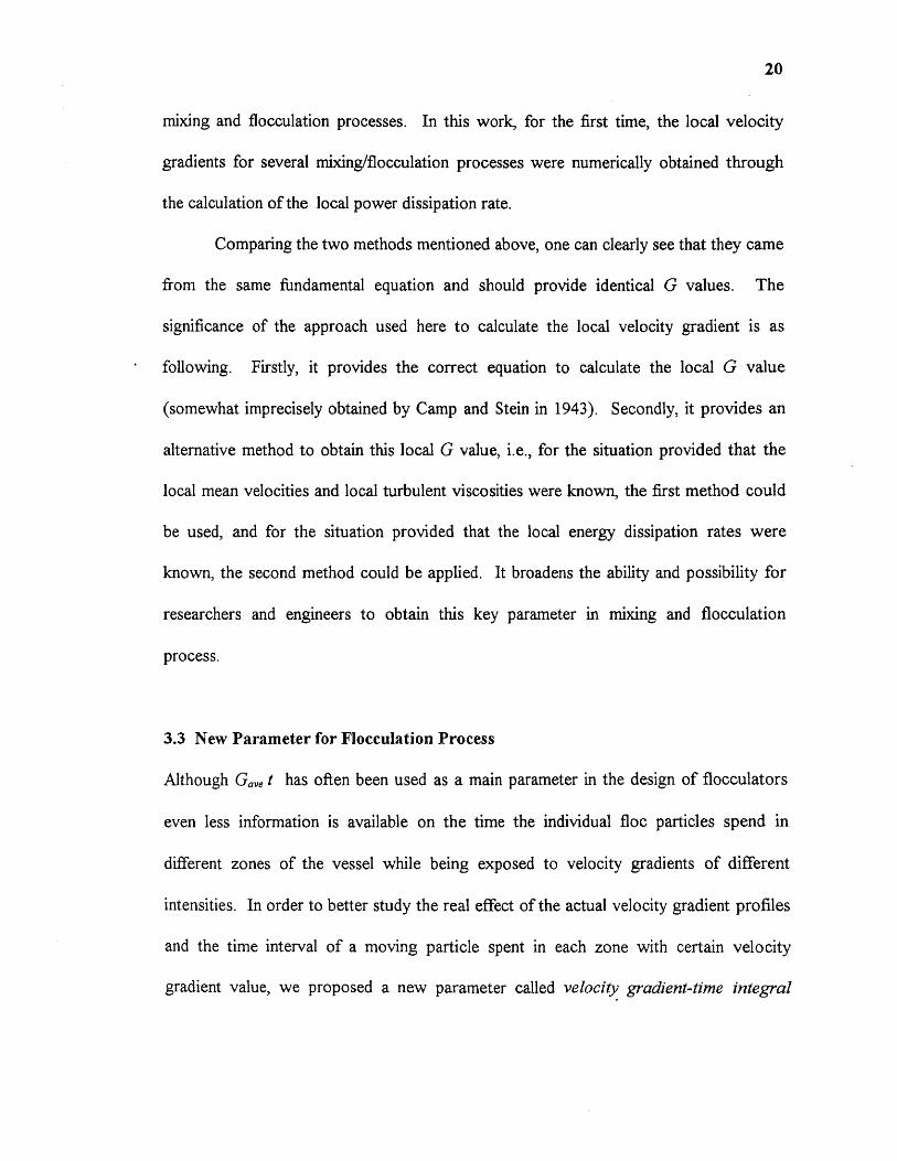
3.3 New Parameter for Flocculation Process
Although Gave t has often been used as a main parameter in the design of flocculators
even less information is available on the time the individual floc particles spend in
different zones of the vessel while being exposed to velocity gradients of different
intensities. In order to better study the real effect of the actual velocity gradient profiles
and the time interval of a moving particle spent in each zone with certain velocity
gradient value, we proposed a new parameter called velocity gradient-time integral

21
along the particle trajectory. This new parameter is the combination of these two factors
(i.e., local velocity gradient, G, and the time a moving particle spent in that cell, t) with
their actual values. To obtain this new parameter for certain flocculation process, firstly,
we need to find the distribution of velocity gradient throughout the entire flocculation
vessel; secondly, we need to track the trajectory of a normal floc particle moving in this
vessel; then finally, we can obtain this new parameter for mixing or flocculation process
through numerically integrating the local velocity gradient value by the time a moving
floc particle spent in that zone of the vessel.
To quantify the velocity gradient-time integral on flocculation it would be
advantageous to be able to measure these quantities directly from experiments and
calculate them from first-principle equations. Until relatively recently this would have
been an extremely difficult task. However, in recent years two tools have become
available to achieve both objectives: Laser-Doppler Velocimetry (LDV) and
Computational Fluid Dynamics (CFD). In this work both tools have been applied to
study the most important fluid dynamic characteristics of mixing and flocculation vessels.

CHAPTER 4
EXPERIMENTAL APPARATUS AND METHOD
The experimental system comprised a mixing vessel, an agitator assembly, an LDV
system, and a data acquisition system. A schematic diagram of the experimental
apparatus is shown in Figure 4-1.
4.1 Mixing and Flocculation Systems
Four mixing and flocculation systems (System A, System B and System Cl and C2,
shown in Fig. 4-2, Fig. 4-3 and Fig. 4-4, respectively) were studied. The study of
System A was a cooperative project between the Department of Chemical Engineering,
Chemistry, and Environmental Science, New Jersey Institute of Technology, Newark,
NJ, USA and the Czech Technical University, Prague, Czech Republic, while the
investigation of System B was a collaborative research project between HSMRC at New
Jersey Institute of Technology, Newark, NJ, USA and Questor Centre at Queen's
University, Belfast, Northern Ireland, U.K.
The agitated vessel in System A was an unbaffled, cylindrical, flat-bottomed,
Plexiglas vessel with a diameter of 0.293 m, provided with a flat lid cover, and
completely filled with water as the process fluid (vessel height = liquid height = 0.293
m). This arrangement suppressed the formation of the central free vortex that can be
typically observed in unbafiled stirred vessels. The vessel was placed in a square
Plexiglas tank filled with water in order to minimize refractive effects at the curved
surface of the mixing vessel. The agitation system consisted of a downward-pumping,
six-blade, 45 ° pitched-blade turbine (Fig. 4-5a) with a diameter of 0.098 m (i.e., equal
22
Dispersion, Prism Collimator
PhotomultiplierAssembly
Laser SP-165-08
1
Mirror
i
/Polarisation
Rotator
\BeamDivider
BraggCell
CompensatingRod Lens
\Vessel
TraversingApparatus
Figure 4-1 Laser-Doppler Velocimetry (LDV) apparatus Square Tank

24
to one-third of the vessel diameter), and a projected vertical blade width of 0.013 m
(corresponding to an actual blade width of 0.019 m). The impeller was mounted 0.073
m off the tank bottom, as measured from the bottom of the impeller. An electric motor
connected to an external controller was used to rotate the impeller at a constant agitation
speed of either 7.5 rotations/s (450 rpm) or 11.67 rotations/s (700 rpm), corresponding
to impeller Reynolds Numbers of 7.1 x10 4 and 11.1 x10⁴ , respectively.
The agitated vessel in System B (presented in Figure 4-3) was a rectangular
mixing tank with the identical configurations to an existing flocculation pilot plant run at
the Questor Centre at Queen's University, Belfast, Northern Ireland, U.K. The flat-
bottomed tank with a square base of 300 mm length and a height of 480 mm was filled
with water to a height of 450 mm. Four baffles with width of 10 mm were placed in the
center of each face of the tank and covered the whole length of the tank. The agitation
system consisted of a radial-pumping, two-blade, paddle type impeller (Fig. 4-5b) with a
diameter of 66 mm and a height of 35 mm. The impeller was mounted 130 mm off the
tank bottom, as measured from the bottom of the impeller. The impeller rotational speed
of 350 rpm (the same rotational speed used in the pilot plant at Queen's University,
corresponding to impeller Reynolds Numbers of 2.5 x10⁴ ) was studied.
System Cl and C2 (shown in Figure 4-4) had the same configuration of System
A except that the vessel had four baffles and did not have a top flat lid cover. The baffle
thickness was 6.25 mm, and the baffle width-to-tank diameter ratio was 0.1. The four
baffles were equally placed along the inner cylindrical surface (i.e. the angle between any
two adjacent baffles was 90 degree) and extended from the top to the bottom of the
25
vessel. Because of the existence of baffles no top flat lid cover is necessary to prevent
vortex normally occurred in unbaffled mixing vessels. The vessel was filled with water
up to a height of 0.293 m and was placed in a square tank, also filled with water, to
minimize the effect of diffraction on LDV measurements. The agitation system consisted
of one downward-pumping, six-blade, 45° pitched-blade turbines mounted on a centrally
located shaft (12.5 mm OD). Two different impeller size were used. One impeller
(System CI) has a diameter 101.6 mm and a vertically projected blade width of 13.7 mm.
Another impeller (System C2) has a diameter 76.2 mm and a vertically projected blade
width of 10.2 mm. The impeller was mounted 0.073 m from the tank bottom for both
System Cl and C2, so that the ratio of the off-bottom clearance of the impeller to the
liquid height was equal to 0.25. The impeller was rotated by the same motor applied in
System B at a speed of 159 rpm and 256 rpm, respectively, corresponding to impeller
Reynolds Numbers of 2.7x10 4 and 2.4x10⁴ for System Cl and C2, respectively. The
three-directional traversing apparatus applied in System B was also used here.
4.2 LDV Systems
The LDV apparatus shown in Figure 4-1 was used to experimentally obtain the velocity
and turbulence intensity profiles inside the vessel. Two similar LDV systems have been
used. One is a 1.5-watt laser (Coherent, Inc.), which has been used for the experimental
measurements in System A by our co-investigators at Czech Technical University,
Prague, Czech Republic. Another one is a 2-watt laser (Lexel, Inc.), which has been
used for the experimental measurements in System B, Cl and C2. Figure 4-1 shows the

26
general diagram for both LDV systems. The multicolor beam produced by the laser in
any of the above two LDV systems passed through the prisms, mirrors, polarization
rotator, and beam divider from which only two colored beam (green and blue) emerged.
Each of these two beams was split into two parallel beams. The resulting four beams
were focused by the beam expander and the final large transmitting lens on a single point
480 mm away from the final lens, i.e., at a distance equal to the focal distance of the final
transmitting lens. The focusing point where the beams converge was actually a small
control volume (84 pin in diameter) formed by the intersection of the four beams. This
point must lie in the fluid contained in the tank under exam to take a velocity
measurement.
The water in the mixing vessel was seeded with metal-coated plastic spheres
(product of TSI Inc.) capable of scattering light as they traveled through the control
volume. These particles, with a density of 1.02 g/cm 3 and mean diameter of 5 pm,
follow the trajectories of the fluid elements very closely. When a particle crossed the
control volume it scattered the light of the incoming beams. This scattered light
produced a light interference pattern that is proportional to the particle velocity. The
back-scattering receiving optics collected the scattered light, and the resulting signal was
sent to a data acquisition system capable of converting it to two values of the velocity
component in two perpendicular directions. The data acquisition system (TSI 1990 A
processor) connected to a computer produced on-line measurements of average and
fluctuating velocities.

27
4.3 Experimental Determination of Velocity Distribution
The tridimensional average and fluctuating velocities in the mixing vessel were
experimentally obtained at 19 radial distances between the impeller shaft and the vessel
wall, and at five different axial levels (Z was equal to 0.053, 0.071, 0.088, 0.160, and
0.233 m, respectively for System A, System Cl; Z was equal to 0.080, 0.128, 0.167,
0.235 and 0.315 m, respectively for System B) using a x-y-z traversing apparatus. The
tridimensional average and fluctuating velocities at only 7 radial positions in the impeller
region at two axial levels (Z was equal to 0.071 and 0.088 m, below and above the
impeller, respectively) were experimentally measured for System C2. To obtain all three
velocity components, two separate measurements were taken for the same (r,Z) point:
one in which the laser axis was oriented perpendicularly to the radius along which the
measurement was made (yielding the radial and axial velocity components), and another
one in which it was parallel (yielding the tangential and axial velocity components),
illustrated by Figure 4-5 (Armenante et aL, 1994).
4.4 Power Number
The torque, 2-, in System A was experimentally measured with a turntable (Fort et al.,
1986), and was used to determine the total power dissipated by the impeller, P, and the
power number, NP, from the equation (Rutherford, 1996) :
27r NN
P=
pN3D 5 pN3D5(4.1)
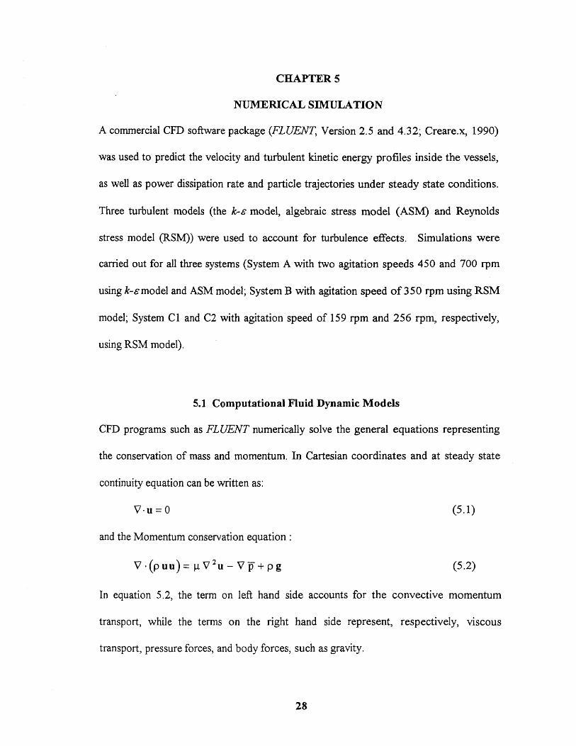
CHAPTER 5
NUMERICAL SIMULATION
A commercial CFD software package (FLUENT, Version 2.5 and 4.32; Creare.x, 1990)
was used to predict the velocity and turbulent kinetic energy profiles inside the vessels,
as well as power dissipation rate and particle trajectories under steady state conditions.
Three turbulent models (the k-s model, algebraic stress model (ASM) and Reynolds
stress model (RSM)) were used to account for turbulence effects. Simulations were
carried out for all three systems (System A with two agitation speeds 450 and 700 rpm
using k-s model and ASM model; System B with agitation speed of 350 rpm using RSM
model; System Cl and C2 with agitation speed of 159 rpm and 256 rpm, respectively,
using RSM model).
5.1 Computational Fluid Dynamic Models
CFD programs such as FLUENT numerically solve the general equations representing
the conservation of mass and momentum. In Cartesian coordinates and at steady state
continuity equation can be written as:
V • u = 0 (5.1)
and the Momentum conservation equation :
V•(puu). p.V 2 u— V + p g (5.2)
In equation 5.2, the term on left hand side accounts for the convective momentum
transport, while the terms on the right hand side represent, respectively, viscous
transport, pressure forces, and body forces, such as gravity.
28
29
In turbulent flow, the velocity at any point can be taken to be the sum of the
mean (time-average) and fluctuating components, i.e.:
u=u+u' (5.3)
Using this equation the continuity equation can be rewritten as:
V • IT = 0 (5.4)
Substitution of equation 5.3 and 5.4 into equation 5.2 yields the ensemble-average
momentum equations, which can be used for the prediction of the velocities in turbulent
flow:
V • (p = ,u V 2 — V p- + p g — V u' u') (5.5)
The last term in this equation represents the Reynolds stresses containing the product of
the fluctuating velocity components.
Since the Reynolds stresses can not be predicted from first principles they are
typically calculated by making some assumptions about their relationship with other
variables. A number of different of models are available for this purpose. Software
packages using some of these models are also available. One of the most widely used
software package is FLUENT. FLUENT includes three turbulence models which can be
used to account for turbulence effects in the simulation. These three models are the k-e
model, the algebraic stress model (ASM) and the Reynolds Stress Model (RSM).
5.1.1 k-eModel
The k- 6. turbulence model is an eddy-viscosity model in which the Reynolds stresses are
assumed to be proportional to the mean velocity gradients, with the constant of

(
Pa c eVc 2+ Gk e
k p 2 (5.9)u • Ve = V••■■•
Gk —pu'ui:(Vu) =au, au,ax ax ;
(5.10)auax
30
proportionality being the turbulent viscosity, . This assumption, known as the
Boussinesq hypothesis, provides the following expression for the Reynolds stresses
(Hine, 1975; Creare.x, Inc., 1991):
dui dui
ax; \
= —2 5,.k + ax;
where cs., is the Kronecker delta and k is the turbulent kinetic energy defined as:
k = —1 (u' •u') (5.7), 2
u, 2 , 2
= -1u + + u2--
\(x Y z2
The values of the specific turbulence kinetic energy, k, and the turbulence energy
dissipation rate, e, were obtained from their balance equations:
u • Vk = V[( 11 '
Pak PVk +
.1 3 p (5.6)
(5.8)
where Gk is the generation of k and is given by:
The effective or "turbulent" viscosity, , is calculated at each point in the flow through
the equation (Rodi, 1984, Creare.x, Inc., 1991):
k 2t = PCp - (5.11)
The values of the constants Ch C2, C, o andcre are taken to be equal to 1.44, 1.92,
0.09, 1.0, and 1.3, respectively (Rodi, 1984).

C D k ( 2u!u'.. k +I 1 3 11 !1 3
— 1 + C 36
(5.12)
31
5.1.2 Algebraic Stress Model (ASM)
In complex flows, pt may be strongly directional. When this is the case, the isotropic k-
e model may be inadequate. For such flows, we can use Algebraic Stress Model (ASM)
or Reynolds Stress Model (RSM). The ASM solves algebraic approximations of the
differential transport equations for the Reynolds stresses as (Rodi, 1984; Fluent. Inc.,
1995):
where (Creare.x, 1991; Launder and Spalding, 1972):
=
and
Qr Oui du,= -u:u; u;ti;
(5.13)
(5.14)
The values of the constants C3, CD are taken to be 0.55, 0.45 respectively (Rodi, 1984).
5.1.3 Reynolds Stress Model (RSM)
RSM involves solving the individual stresses ul ul in differential transport equations.
The following equations are used (Launder, et al., 1975; Launder, 1989; Fluent. Inc.,
1995):
au.u. a v t au i ujU k Pii + - e + R
k ax k axk(5.15)

32
where the term on the left hand side is the convective momentum transport. The first
term on the right hand side is the diffusive transport, is the stress production rate, (Dii
correlates the pressure/strain, eij is the viscous dissipation and Ri; is the rotational term,
v t is the turbulent kinematic viscosity.
5.2 Boundary Conditions
The boundary conditions imposed on the systems are as follows. The boundary
conditions at the horizontal top for System A and the vessel wall, baffles, horizontal
bottom for all systems were those derived assuming no-slip condition. This implied that
the shear stress near the solid surfaces is specified using wall functions and that
equilibrium between the generation and dissipation of turbulence energy is assumed
(Launder and Spalding, 1974; Ranade et al., 1989). The boundary conditions at the top
(free surface) for System B, Cl and C2 are of the zero-gradient, zero-flux type, which is
equivalent to a frictionless impenetrable wall. The common symmetry boundary
conditions are assumed at the symmetry axis for all systems (Ranade et al., 1989).
The boundary conditions in the impeller region are imposed at two surfaces of the
cylinder having the same size of the volume swept by the impeller. The boundary time-
averaged velocities in all three directions are directly obtained from LDV data. The
turbulent kinetic energies at the same locations are determined from the experimental
fluctuating velocities using equation 5.7, whereas e is calculated from:
k 1.56 = a (5.16)

33
where w is the projected blade width (along the vertical axis), and a was taken to be
equal to 1.4 (Wu and Patterson, 1989; Armenante et al., 1994). The values of the
average velocities, k and e so obtained were directly used in the simulations as impeller
boundary conditions.
For the System A, the average and fluctuating velocities were experimentally
determined via LDV at 9 radial locations 2 mm below and 2 mm above the impeller
surface (corresponding to Z values equal to 0.071 and 0.088 In, respectively) by our co-
investigators Ivan Fort (Faculty of Mechanical Engineering, Czech Technical University,
Prague, Czech Republic) and Jaroslav Medek (Faculty of Mechanical Engineering,
Technical University, Brno, Czech Republic). For System B, the average and
fluctuating velocities were experimentally determined via LDV at 7 radial locations 2
mm below and 2 mm above the impeller surface (corresponding to Z values equal to
0.128 and 0.167 m, respectively) in the Mixing Lab at New jersey Institute of
Technology. For System Cl and C2, 9 points and 7 points, respectively, were
experimentally measured at the same two levels as in System A.
5.3 Grid Generation
FLUENT provides a x-window interface for grid generation. According to the research
purpose and results requirements, different grid and domain for certain type of mixing
systems could be used. For the System A, a repeating 60 ° domain was selected, and a
non-uniform grid composed of 30 radial nodes, 40 axial nodes, and 17 tangential nodes
was imposed on this domain. The grid was chosen to be finer (smaller volume of
QC = 2 rr S I% 112 01 rdr +n-D ur (Z)o Z=ZbdZ (5.18)
r.—
34
computational cell) in the region near the impeller. For System B, the entire mixing
vessel (360° domain) was chosen, because of the asymmetry characteristic of the flow in
the vessel. Cartesian coordinates were used for System B. A non-uniform grid with
about 49,000 computational cells was generated for the simulation. For System Cl and
C2, a repeating 90° domain was selected because of the cyclic characteristic of flow in
the vessel and the presence of four baffles. A non-uniform grid with finer grid (smaller
volume of computational cell) near the impeller region was generated. About 40,000
computational cells were applied for this domain during the CFD simulation.
5.4 Power Consumption and Pumping Capacity
The overall power consumption (P) was calculated for System A by numerically
integrating the local power consumption (obtained as the product of the numerically
determined local e value and the fluid mass of each cell) over the entire vessel, as:
P = e dm ecell mcen (5.17)m cell i
The pumping capacity, Q c, was obtained by numerical integration of the numerically
obtained velocities in the impeller region (Armenante and Chou, 1996), as follows:
The dimensionless flow number, Fl, is defined as the pumping capacity through the
impeller zone, Qc, normalized by ND3 and then be calculated from:
Fl Qc
ND 3(5.19)
35
5.5 Local G Value Calculation
After the CFD simulation is complete, FLUENT can produce the mean velocity
components at all three directions, the effective viscosity and the energy dissipation rate
in any location throughout the agitated vessel. Using these data we were able to
calculate the local G value distribution within the vessel with the rigorous methods
described in chapter 3 (the complete definition of local velocity gradient method and the
local energy dissipation rate method).
The general procedure to calculate the local G value is as follows. For the
complete definition of local velocity gradient method, we downloaded the data output
file from FLUENT containing the local mean velocity components in all three directions,
i.e. the ur (tangential), ur (radial) and ua (axial) velocities for cylindrical coordinates or
the ux ,uy, u, velocities for cartesian coordinates, as well as the effective viscosity at any
position within the vessel. The above data were imported into MS Excel spreadsheets.
A macro program (Appendix B) was written using Visual Basic language in order to
compute all the differential terms in Eq. 3.21 (for cartesian coordinates) or Eq. 3.22 (for
cylindrical coordinates). The derivatives were calculated as the ratios of the differences
of the velocities between two adjacent cells to the distances between the same cells. By
summing the squared derivative terms according to Eq. 3.21 or Eq. 3.22, and
multiplying by the coefficient in these equations (the ratio of effective viscosity to the
dynamic viscosity), the local G value at any position was numerically obtained.
For the calculation of the local energy dissipation rate method, we downloaded
the data output file from FLUENT with the information of local energy dissipation rate
181.1. C D Re
p pD: 24(5.21)
36
at any position within the vessel. Then the above data file was imported into MS Excel
spreadsheets, where the local G value at any position within the vessel was calculated by
a macro program (Appendix C) based on the Eq. 3.24. Therefore the local G value
distribution was numerically determined.
5.6 Particle Trajectory
FLUENT can determine the trajectory of a dispersed phase particle by integrating the
force balance on the particle in a Lagrangian reference frame. This force balance
equates the particle inertia with the forces acting on the particle, and can be written (for
the x-direction in Cartesian coordinates) as:
du p FD gx(p p p)/ pdt
(5.20)
where gr(A, p)/p is the body force; FD is the drag force per unit particle mass and:
Here, u is the fluid phase velocity, up is the particle velocity, p is the molecular viscosity
of the fluid, p is the fluid density, pp is the density of the particle, and Dp is the particle
diameter. Re stands for the relative Reynolds number, which is defined as:
Re = PD P 141 (5.22)
The drag coefficient, CD , is a function of the relative Reynolds number of the following
general form:
CD = a1 + a2/ Re + a3 / Re2 (5.23)
F x = --12-11u) p ) Ox
(5.25)
37
where the a's are constants that apply over several ranges of Re given by Morsi and
Alexander (1972).
In equation 5.20, the term Fx represents some additional forces that can be
important under special circumstance. The first of these is the "virtual mass" force, the
force required to accelerate the fluid surrounding the particle. This force can be written
as:
F _ _lp d(u __\— 2 p p dt " )
and is important when p > p p .
(5.24)
Another additional force may arise due to the pressure gradient in the fluid:
These forces are optional when using FLUENT.
The trajectory equation can be numerically integrated by FLUENT to produce
the velocity of the particle at each point along the trajectory, where the trajectory itself
is obtained through the following equation:
d xu = (5.26)Pi d t
i.e.
x =j. u Pi d t (5.27)
38
Therefore, the position of a moving particle at any time can be tracked by
simulation method. During the simulation, the density and diameter of the moving
particle were chosen to be 1.0 g/cm3 and 100 pm, repectively.
5.7 Local G Value Distribution Along a Particle Trajectory
After certain number of iterations (depending on the total number of computational cells
and boundary conditions), FLUENT output the converged results including the local
mean velocities in three directional components, turbulent kinetic energy, turbulent
viscosity and energy dissipation rate at each cell within the entire vessel. By
downloading the output file composed of mean velocities of three components and local
turbulent dissipation rate from FLUENT, importing it into Excel spreadsheet and using
Eq. 3.16 or 3.17 for the complete definition of local velocity gradient method (by
computing the derivative between two adjacent positions for each term on the right hand
side of above equation) or Eq. 3.20 for local energy dissipation rate method, the
distribution of local velocity gradient (G value) was obtained throughout the entire
vessel. Two macro programs, listed in Appendix B and C, were developed to calculate
the local velocity gradient through both methods. These macros were written by using
Visual Basic language in Microsoft Excel 5.0. When particle trajectory simulation was
complete, FLUENT produced the trajectory of a dispersed particle with the output of its
location (its corresponding x, y, z or radial, tangential, axial values, in cartesian or
cylindrical coordinates, respectively), its velocity components in three directions at that
position and its corresponding time. The output file from FLUENT was downloaded and
velocity gradient-time integral = f G( x, y, z )dt =G(s)
dsu
t o 0 P ( s )
39
then imported into Excel spreadsheet together with the above obtained local G value
distribution data. The macro program (attached in Appendix C) can also calculate the
corresponding G value at different times (corresponding to different particle positions).
Thus the G value distribution along the particle trajectory could be obtained.
5.8 Velocity Gradient-Time Integral
Knowing the particle trajectory, the velocity of particle at each point and the G value
distribution along the particle trajectory, it was then possible to calculate the new
parameter - the velocity gradient-time integral along the particle trajectory - from the
following equation:
(5.28)
where the variable s is the linear coordinate along the trajectory and up(s) is the particle
velocity along the trajectory. A macro program was written to calculate the time
interval the moving particle spent at different G value zone and the value for the new
parameter velocity gradient-time integral (Appendix C).
CHAPTER 6
RESULTS AND DISCUSSION
6.1 System A
For the unbaffled cylindrical mixing system with both agitation speeds of 450 rpm and
700 rpm, LDV was used to measure both the average and fluctuating velocities in all
three directions at 5 different axial levels by our co-investigators at the Czech Technical
University, Prague, Czech Republic. Then these experimentally obtained data (via LDV)
near the impeller region were used as the boundary conditions when the CFD program
FLUENT was used to numerically simulate the flow pattern in this mixing vessel. Two
turbulence models (k-e and ASM) were used in the simulation to account for the
turbulence effect. The results of both LDV measurements and CFD predictions are
presented in the following sections.
6.1.1 LDV Measurements in the Impeller Region
It has been a common procedure to present the standardized local values of mean and
fluctuating velocities by relating their original values to the impeller tip speed (7cD.N).
The velocities in these figures, as well as in all other velocities profiles in this work, are
presented in a dimensionless form by dividing the actual value by the impeller tip
velocity. The turbulent kinetic energy is also presented in a dimensionless form by
dividing the actual value by the square of impeller tip velocity.
Figures 6-la and 6-lb show the velocities in the impeller region obtained via
LDV. The tangential velocity profiles show a maximum near the tip of the impeller.
This pattern is consistent with that reported for a system similar to that under study
40

41
(Armenante et al., 1994) as well as for an unbaffled tank without a lid using a flat-blade
paddle (Nagata, 1975), or an eight-blade, flat-blade turbine (Doug et al., 1994a and
1994b). The axial velocities above and below the impeller are all negative, as one would
expect for a downward pumping impeller. However, the velocities above the impeller
are quite low and uniform, whereas those below the impeller show a strong downward
pumping action near the outer edge of the impeller. The radial velocities point slightly
inward above the impeller but strongly outward on the lower side of the impeller.
The turbulent kinetic energy profiles for the impeller region are given in Figure 6-
1c. k is greatest on the lower side of the impeller near the tip, where the radial velocity is
also the greatest. An overall lower distribution of k can be observed on the upper side of
the impeller where the average velocities are more uniform.
The values for the velocity components (radial, tangential and axial) and for k
shown in the above figures were used as boundary conditions for the numerical
simulation resulting in the velocity profiles inside the vessel.
A repeating 60° domain was selected for the CFD simulation, and a non-uniform
grid composed of 30 radial nodes, 40 axial nodes, and 17 tangential nodes was imposed
on this domain. The grid was chosen to be finer in the region near the impeller to obtain
better simulation results. Figure 6-2 and 6-3 show the grid in 2D and 3D view,
respectively.
42
6.1.2 Comparison between LDV Measurements and CFD Predictions
A comparison between the experimental tangential velocities and the results of the CFD
simulations is given in Figure 6-4. The results of the simulation based on the ASM
model were, in general, superior to those based on the k-c model. The agreement
between the experimental data and the ASM simulation velocities was very good in the
planes next to, or lower than, the impeller. Good agreement can be observed also for the
velocities on the other two planes above the impeller, but only for radial distances
greater than the impeller radius. For r < D/2 the agreement in these regions was
qualitatively but not quantitatively acceptable.
Figure 6-5 shows that a very good agreement between the numerical and
experimental results was also obtained for the axial velocity. Near the vessel bottom the
simulation typically overpredicted the experimentally determined velocities. However, it
should be remarked that the reproducibility of the LDV velocity results in the region
below the impeller was not as good as in the rest of the vessel, most likely because of the
lower values of the velocities and the instabilities of the secondary flow pattern (radially
inward and axially upward) typically observed just below pitched blade turbines.
The corresponding velocity data in the radial direction are given in Figure 6-6.
While the experimental velocities above the impeller are predicted satisfactorily those
below the impeller are only qualitatively described by the results of the simulations.
Discrepancies exist especially near the center of the vessel, although the curves produced
by the simulations show a trend similar to that of the experimental data.

43
The ultimate test of the appropriateness of the turbulence models used in the
simulation is in the agreement between the experimental and predicted turbulent kinetic
energy data. This comparison, shown in Figure 6-7, indicates that ASM is clearly
superior to the k-e model. The experimental k values above the impeller are closely
matched by the results of the ASM simulation, whereas those based on the k-e model are
significantly off the mark. Significant qualitative agreement exists also for the results
below the impeller, but only when the results of the ASM simulation are compared to the
experimental data. The inability of results from the simulation with the k-4 model to
match the experimental data can be attributed to the local isotropic assumption made in
the derivation of this model.
The overall circulation pattern generated by the simulation is captured in Figures
6-8a (in three dimensions) and 6-8b (in a two-dimensional plane through the shaft). The
flow pattern in the r-Z plane is dominated by the main flow generated by the impeller,
initially strongly directed outward in the radial direction, and to a lesser extent,
downward. This flow rapidly becomes horizontal (for r > T/4) although the impeller
used here is not of the radial type.
Two main recirculation flows, one above and the other below the impeller, can be
clearly identified in Figure 6-8b. In general, the magnitudes of the velocity vectors in the
r-Z plane outside the impeller stream are small in comparison to those outside this zone,
generating large regions in which axial and radial recirculation is limited (such as the
upper region for r > T/4). In the region just above the impeller the flow in the r-Z plane
is mainly directed straight downward, feeding the impeller. In the cylindrical region

44
immediately adjacent to the shaft the numerically predicted velocity vectors are very
small. This is likely to be an artifact of the computer simulation produced by the absence
of boundary condition data in the impeller region for r < 0.075•T. The region just below
the impeller is nearly completely cut off from the main lower circulation flow. Figure 6-
8b shows that the velocity vectors are quite small in both the radial and axial directions.
It is interesting to compare the flow simulation produced here with that reported
for the same type of turbine in a baffled system (Armenante and Chou, 1996, their Figure
8). In the baffled system the main flow generated by the impeller had a very strong
downward component, resulting in this flow impinging on the bottom of the vessel and
then moving upward near the tank wall. In that system the pitched-blade turbine
performed as an effective axial impeller (except for the region just below the impeller in
which flow reversal can be noticed). A single large recirculation flow in the axial
direction was present, which can be expected to provide good top-to-bottom mixing. By
contrast in the unbaffled system examined here top-to-bottom recirculation appears to be
modest, and the pitched-blade impeller loses most of the axial impeller characteristics
that it typically exhibits in baffled systems.
A comparison among Figures 6-4, 6-5, and 6-6 reveals that the tangential
velocities in the unbaffled tank are several times greater in magnitude than the
corresponding axial and radial velocities. This is not the case for the baffled case for
which the velocity vectors have comparable magnitude independently of the direction
(Armenante and Chou, 1996). Figure 6-4 also shows that the magnitude of the
45
tangential velocities is nearly independent of the axial position, indicating the presence of
a very strong swirling flow not observed in the baffled system.
In Table 6-1 the power numbers and the flow number for the system are
reported. For the 450 rpm case, the power number prediction based on ASM (0.304)
could only account for 65.7% of the experimentally obtained power number, whereas
that based on the k-s model (0.482) was very close to the experimental value. The flow
number could only be obtained numerically since the velocities at the vertical side of the
volume swept by the impeller were not measured. The value so obtained (0.391)
compares favorably with the value (0.31) experimentally obtained by Nagata and
coworkers (as reported by Gray, 1966) for the case of an 8-blade flat-blade turbine
having the same blade-to-diameter ratio as that of the impeller used in this work.
6.1.3 Comparison between Different Agitation Speeds
Experimental results and simulations for the velocity distributions were obtained for the
case in which the agitation speed was increased to 700 rpm. The results are reported in
Figures 6-9 (boundary conditions in the impeller region), 6-10, 6-11, 6-12 (dimensionless
velocity components in three directions), and 6-13 (dimensionless turbulent kinetic
energy). The striking feature of all these figures is that they are all nearly
superimposable to the corresponding figures obtained at 450 rpm, indicating that the
impeller speed plays a minor role in the direction and magnitude of the dimensionless
velocities and turbulent kinetic energies at any point (including the region near the
impeller). Similar conclusions were reached by Dong et al. (1994a) for an
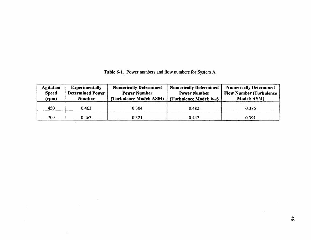
Table 6-1. Power numbers and flow numbers for System A
AgitationSpeed(rpm)
ExperimentallyDetermined Power
Number
Numerically DeterminedPower Number
(Turbulence Model: ASM)
Numerically DeterminedPower Number
(Turbulence Model: k-e)
Numerically DeterminedFlow Number (Turbulence
Model: ASM)
450 0.463 0.304 0.482 0.386
700 0.463 0.321 0.447 0.391
47
open unbaffled system provided with a flat-blade impeller. These results indicate that the
potential exists for simple scale-up rules for the velocity distribution and the turbulence
intensity in unbaified tanks. As for the power number and the flow number Table 6-1
shows that both non-dimensional numbers had values very similar to those obtained at
450 rpm.
Although no experiments were conducted here at different scales it is conceivable
that non-dimensional velocity and k value profiles nearly identical to those found here
would be obtained in a geometrically similar system of a different scale (since the
presence of a lid would eliminate any vortex and the scale up problems associated with
it). Identical dimensionless conditions in the impeller region are equivalent to identical
boundary conditions, and hence identical simulation results. Given the good agreement
between the experimental data and the simulation results obtained here with ASM it
follows that the flow in the full-scale vessel is likely to be correctly simulated by the
figures reported in this work.
6.2 System B
For the baffled rectangular mixing/flocculation system with agitation speed of 350 rpm,
tridimensional average and fluctuating velocities at 5 different axial levels were
experimentally measured via LDV in the Mixing Laboratory at the Department of
Chemical Engineering, Chemistry, and Environmental Science, New Jersey Institute of
Technology. Then these experimentally obtained data near the impeller region were used
as the boundary conditions when the CFD program FLUENT was used to produce a

48
numerical estimate of the velocity distribution, turbulence kinetic energy, the energy
dissipation rate, local velocity gradient distribution and particle trajectory in this
mixing/flocculation vessel. One turbulence models (RSM) was used in the simulation.
During the CFD simulation process, Cartesian coordinates were used, where the
velocities in the three directions were expressed as x, y, z direction velocities. In order
to give more intuitive expression of these data (relating them to the tip velocity of the
impeller) and make them consistent with the previous results for System A, these data (in
Cartesian coordinates) were then transformed into cylindrical coordinate data, where the
three directional velocities were expressed as axial, radial and tangential velocities
respectively, as shown in the following sections.
6.2.1 LDV Measurements in the Impeller Region
The velocities in the tangential, axial, and radial directions were experimentally
determined via LDV for the top and bottom layers (at the vertical plane along the shaft
center and the baffle) of the cylindrical region swept by the impeller. These
experimentally determined velocities are reported in Figures 6-14a and 6-14b. Each
point in these figures represents the average of three measurements. The results of these
figures indicate that the flow in the impeller region had a strong radial component across
the entire top and bottom surface of the impeller region, and that this velocity had a
numerical value approximately in the range 0.16-0.38 of the impeller tip speed ('rDN).
The radial velocity increased as the distance between the measuring point and the central
line of the shaft became larger, and reached its highest value of about 0.38 of the
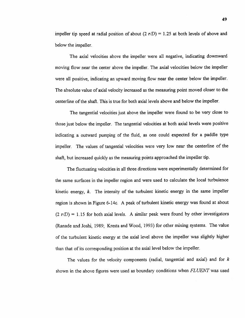
49
impeller tip speed at radial position of about (2 r/D) = 1.25 at both levels of above and
below the impeller.
The axial velocities above the impeller were all negative, indicating downward
moving flow near the center above the impeller. The axial velocities below the impeller
were all positive, indicating an upward moving flow near the center below the impeller.
The absolute value of axial velocity increased as the measuring point moved closer to the
centerline of the shaft. This is true for both axial levels above and below the impeller.
The tangential velocities just above the impeller were found to be very close to
those just below the impeller. The tangential velocities at both axial levels were positive
indicating a outward pumping of the fluid, as one could expected for a paddle type
impeller. The values of tangential velocities were very low near the centerline of the
shaft, but increased quickly as the measuring points approached the impeller tip.
The fluctuating velocities in all three directions were experimentally determined for
the same surfaces in the impeller region and were used to calculate the local turbulence
kinetic energy, k. The intensity of the turbulent kinetic energy in the same impeller
region is shown in Figure 6-14c. A peak of turbulent kinetic energy was found at about
(2 r/D) = 1.15 for both axial levels. A similar peak were found by other investigators
(Ranade and Joshi, 1989; Kresta and Wood, 1993) for other mixing systems. The value
of the turbulent kinetic energy at the axial level above the impeller was slightly higher
than that of its corresponding position at the axial level below the impeller.
The values for the velocity components (radial, tangential and axial) and for k
shown in the above figures were used as boundary conditions when FLUENT was used

50
to predict the velocity and velocity gradient distribution as well as the trajectory of a
particle moving in this vessel.
When generating the grid, the entire mixing vessel (360° domain) was chosen,
because of the asymmetry characteristic of the flow in the vessel. A non-uniform grid
with 49,000 computational cells was generated for the simulation, shown in Figure 6-
15(2D view) and Figure 6-16 (3D view).
6.2.2 Comparison between LDV Measurements and CFD Predictions
The results of the numerical simulation, as well as the values of the three experimentally
determined velocity components in the bulk of the fluid obtained at five vertical levels
(at the vertical plane along the shaft and the baffle) are presented in Figures 6-17, 6-18,
and 6-19. Figure 6-17 shows a comparison between the experimental data for the
tangential velocities at different positions inside the vessel and the corresponding values
obtained from the numerical simulation by using FLUENT RSM model. One can see
that the agreement is quite good for all the cases examined here (i.e., all the different Z/H
values). A peak of the tangential velocity was found near the impeller tip for both axial
levels above and below impeller, with the value of 0.28 impeller tip velocity. The
tangential velocities were found to be higher near the impeller and its adjacent region
than the other regions within the vessel. The much lower values of the tangential
velocities at the bottom level (Z=80 mm) and top level (Z=315 mm) indicate that almost
no swirl flow exists at both the top and bottom of the vessel.

51
A comparison between experimental and simulation results is also provided for
the axial velocity component for the same Z/H values (Figure 6-18). Significant
agreement was obtained for all levels. This figure shows that below the impeller near the
vessel wall, the axial velocity is directed downwards and near the vessel center, the axial
velocity is directed upwards, indicating a main recirculation exist below the impeller. It
also shows that above the impeller near the vessel wall, the axial velocity is directed
upwards and near the shaft center, the axial velocity is directed downwards, indicating
another main recirculation exist above the impeller.
A very good agreement between the experimentally determined radial velocities
and the values obtained through FLUENT simulation at the same 5 Z/H levels is shown
in Figure 6-19. Positive peak values were observed for the axial levels just above and
below the impeller. The highest radial velocity with the value of about 0.4 impeller tip
velocity was found at about (2 r/7) = 0.28 on both levels of above and below the
impeller. The negative values of radial velocity at the other three axial levels indicating
an inwards moving flow both near the bottom and top of the vessel.
Figure 6-20 presents a comparison between the experimental dimensionless
turbulent kinetic energies and the corresponding values produced using FLUENT. It is
seen that the predictions fit the experimental measurements quite well. The values of
turbulent kinetic energies near the impellers are much higher than those at the rest of the
vessel. A peak was found near the impeller tip.
Figure 6-21 shows a bidimensional cross-sectional view of the velocity profiles
on a plane passing through the impeller shaft obtained via simulation. A tridimensional
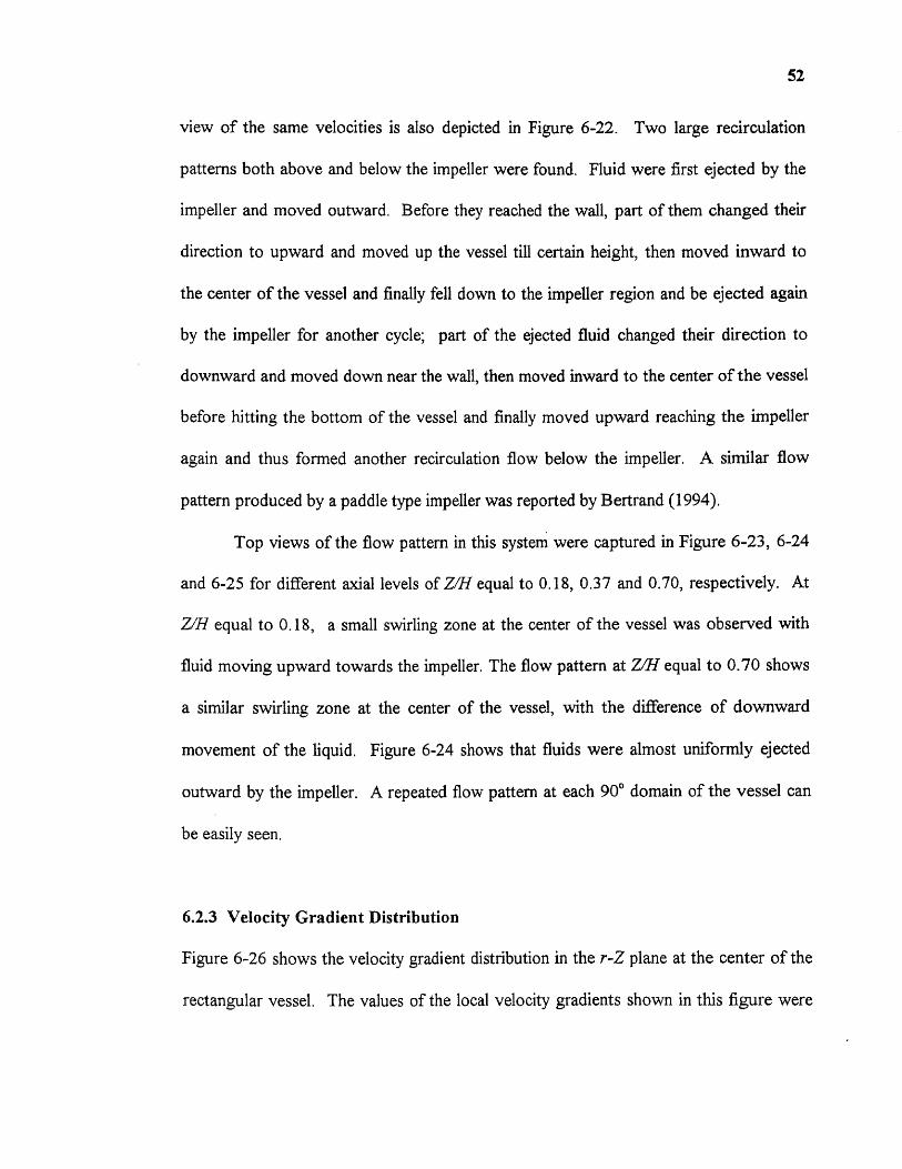
52
view of the same velocities is also depicted in Figure 6-22. Two large recirculation
patterns both above and below the impeller were found. Fluid were first ejected by the
impeller and moved outward. Before they reached the wall, part of them changed their
direction to upward and moved up the vessel till certain height, then moved inward to
the center of the vessel and finally fell down to the impeller region and be ejected again
by the impeller for another cycle; part of the ejected fluid changed their direction to
downward and moved down near the wall, then moved inward to the center of the vessel
before hitting the bottom of the vessel and finally moved upward reaching the impeller
again and thus formed another recirculation flow below the impeller. A similar flow
pattern produced by a paddle type impeller was reported by Bertrand (1994).
Top views of the flow pattern in this system were captured in Figure 6-23, 6-24
and 6-25 for different axial levels of Z/H equal to 0.18, 0.37 and 0.70, respectively. At
Z/H equal to 0.18, a small swirling zone at the center of the vessel was observed with
fluid moving upward towards the impeller. The flow pattern at Z/H equal to 0.70 shows
a similar swirling zone at the center of the vessel, with the difference of downward
movement of the liquid. Figure 6-24 shows that fluids were almost uniformly ejected
outward by the impeller. A repeated flow pattern at each 90° domain of the vessel can
be easily seen.
6.2.3 Velocity Gradient Distribution
Figure 6-26 shows the velocity gradient distribution in the r-Z plane at the center of the
rectangular vessel. The values of the local velocity gradients shown in this figure were

53
obtained through the method of complete definition of local velocity gradient. The labels
of the contour curves in this figure are the G values in the form of logioG. It is clear that
significant variations in the local velocity gradient exist in the vessel. The velocity
gradient values near the vessel wall were very low, only around 10 s-1 . They increase as
the interested position moves close to the impeller. The closer the position to the
impeller, the higher the G value. The highest values were found just near the impeller. It
is obvious that the velocity gradient distribution within a agitated vessel is far from
uniform.
Figure 6-27 maps the local velocity gradient distribution, obtained through the
local energy dissipation rate, in the r-Z plane at the center of the rectangular vessel in the
same agitated vessel as in Figure 6-26. Comparing Figure 6-26 and Figure 6-27, one
will find that the values obtained by these two different methods at corresponding
position within the vessel were of the same magnitude. The relatively small value
differences existed here were brought from the numerical calculation process, as one
could expect. In general, they provide the same information about the distribution of
local velocity gradient in the turbulent mixing/flocculation process. This convinced us of
the validity of the second method (by local energy dissipation rate), derived from a
modified Camp and Stein (1943) approach to G determination.
Similarly to what it was found in this work, Geisler and Forschner (1996) found
that "Maximum values of 8 are always in the discharge region of the impeller" when they
studied the local turbulent shear stress for different mixing tanks. Stanley and Smith
(1995) also found that "the local dissipation rate in the impeller zone is 4-6 times higher
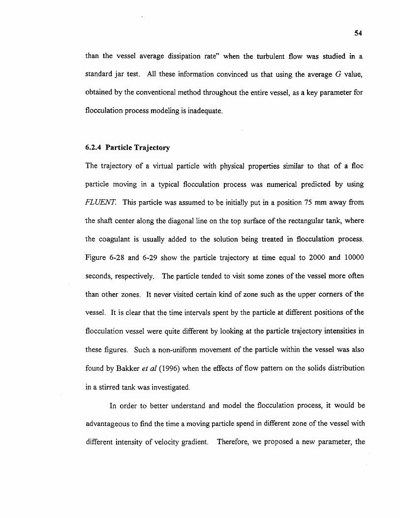
54
than the vessel average dissipation rate" when the turbulent flow was studied in a
standard jar test. All these information convinced us that using the average G value,
obtained by the conventional method throughout the entire vessel, as a key parameter for
flocculation process modeling is inadequate.
6.2.4 Particle Trajectory
The trajectory of a virtual particle with physical properties similar to that of a floc
particle moving in a typical flocculation process was numerical predicted by using
FLUENT This particle was assumed to be initially put in a position 75 mm away from
the shaft center along the diagonal line on the top surface of the rectangular tank, where
the coagulant is usually added to the solution being treated in flocculation process.
Figure 6-28 and 6-29 show the particle trajectory at time equal to 2000 and 10000
seconds, respectively. The particle tended to visit some zones of the vessel more often
than other zones. It never visited certain kind of zone such as the upper corners of the
vessel. It is clear that the time intervals spent by the particle at different positions of the
flocculation vessel were quite different by looking at the particle trajectory intensities in
these figures. Such a non-uniform movement of the particle within the vessel was also
found by Bakker et al (1996) when the effects of flow pattern on the solids distribution
in a stirred tank was investigated.
In order to better understand and model the flocculation process, it would be
advantageous to find the time a moving particle spend in different zone of the vessel with
different intensity of velocity gradient. Therefore, we proposed a new parameter, the

55•
velocity gradient-time integral, which accounts for both the local velocity gradient
distribution and the time a particle spend in each of those zones with certain G value.
6.2.5 Velocity Gradient-Time Integral along the Particle Trajectory
By knowing the local velocity gradient distribution within the entire mixing/flocculation
vessel and the trajectory of a particle moving in this vessel, we were able to calculate the
proposed new parameter, the velocity gradient-time integral along the particle trajectory.
Using the macro program attached in appendix C, the local G value at each point
the particle went through during the flocculation process was obtained. The result is
shown in Figure 6-30, where the x coordinate represents the time a moving particle spent
in the vessel and the y coordinate represents the local G value the moving particle
experienced. It is clear that the G value experienced by the particle as it moves through
the vessel is extremely non-uniform. Very high peaks were calculated (when the particle
moved through the impeller region), followed by long periods during which the G values
were extremely low. The dotted line shown in Figure 6-30 is the average G value
obtained through the conventional method for the entire flocculation vessel. Obviously,
the use of average G value throughout the entire vessel by the conventional method is a
very crude estimation of the actual flocculation characteristics.
Besides the distribution of the local velocity gradient in flocculation vessel it is of
great interest to pay attention to the maximum values of the local velocity gradient the
particle experienced. In this flocculation system the maximum value of the local velocity
gradient the particle experienced is about 920 s' 1 , as shown in Figure 6-30. If the
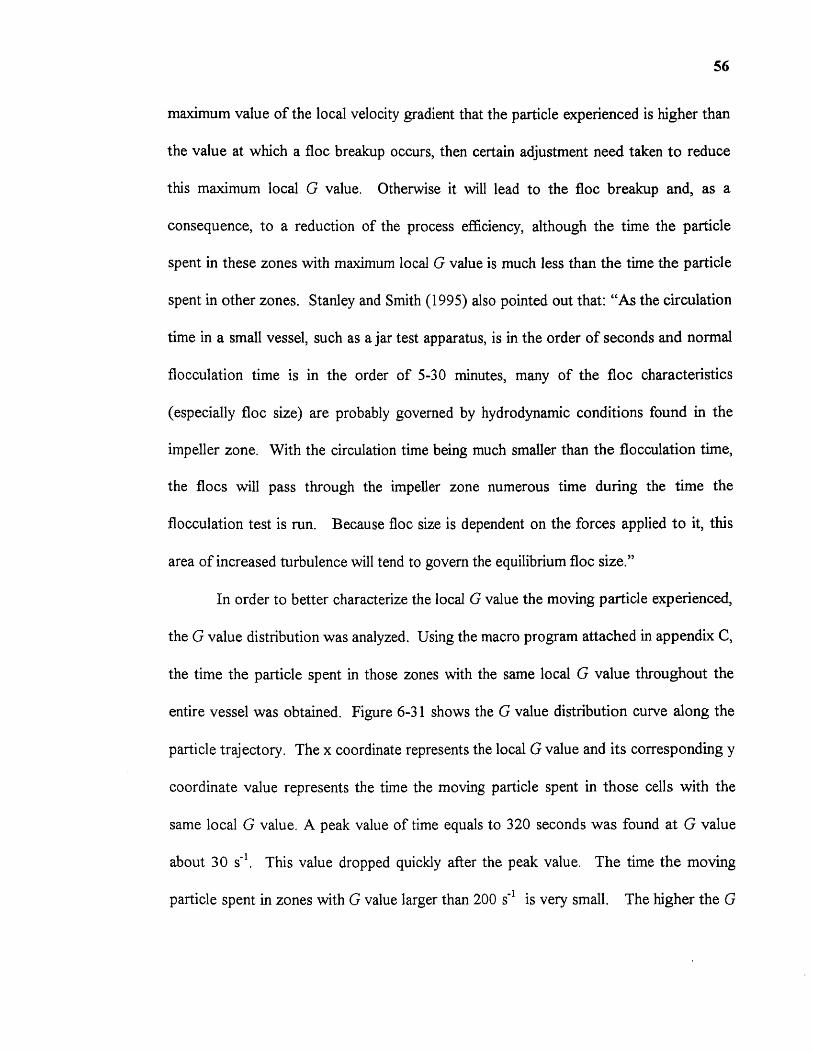
56
maximum value of the local velocity gradient that the particle experienced is higher than
the value at which a floc breakup occurs, then certain adjustment need taken to reduce
this maximum local G value. Otherwise it will lead to the floc breakup and, as a
consequence, to a reduction of the process efficiency, although the time the particle
spent in these zones with maximum local G value is much less than the time the particle
spent in other zones. Stanley and Smith (1995) also pointed out that: "As the circulation
time in a small vessel, such as a jar test apparatus, is in the order of seconds and normal
flocculation time is in the order of 5-30 minutes, many of the floc characteristics
(especially floc size) are probably governed by hydrodynamic conditions found in the
impeller zone. With the circulation time being much smaller than the flocculation time,
the flocs will pass through the impeller zone numerous time during the time the
flocculation test is run. Because floc size is dependent on the forces applied to it, this
area of increased turbulence will tend to govern the equilibrium floc size."
In order to better characterize the local G value the moving particle experienced,
the G value distribution was analyzed. Using the macro program attached in appendix C,
the time the particle spent in those zones with the same local G value throughout the
entire vessel was obtained. Figure 6-31 shows the G value distribution curve along the
particle trajectory. The x coordinate represents the local G value and its corresponding y
coordinate value represents the time the moving particle spent in those cells with the
same local G value. A peak value of time equals to 320 seconds was found at G value
about 30 s-1 . This value dropped quickly after the peak value. The time the moving
particle spent in zones with G value larger than 200 s 4 is very small. The higher the G

57
value, the shorter the time the moving particle spent in those zones. It is quite evident
that the local residence time or, vice versa, the residence probability of a particle is much
smaller in zones of high velocity gradient (near the impeller region) than in zones far
away from the impeller blades, because the local fluid velocities differ greatly between
the direct discharge area and zones far away from the impeller blades.
The cumulative G value distribution along the particle trajectory was also
obtained and is presented in Figure 6-32. At the beginning, the cumulative time spent by
the moving particle increase dramatically as G value increase. It slowed down when the
G value reached about 60 s4 and almost kept a stable value after G value is larger than
200 s-1 . This again indicates that the time the particle spent in those zones with high G
value was much less than the other zones with low G value.
Knowing the distribution of local G value the particle experienced along its
trajectory, the new parameter proposed in this work was calculated. Multiplying the
local G value by the time the moving particle spent in a cell and integrating this value as
a function of time produces the numerical value of this new parameter. Figure 6-33
shows the numerical integration of this new parameter vs. the time the particle spent in
the entire vessel. As the time added up, the value of this integration increased steeply at
the first 100 seconds and then slowly. The moving average of the G value along the
particle trajectory is presented in Figure 6-34 as a function of time. This average G
value was obtained by dividing the previously obtained velocity gradient-time integral by
the time spent by the particle up to that point. This average G value fluctuated at the
beginning of the process when the total time was less than 400 seconds and then reached
58
an almost constant value of 29 indicating the possibility that this new parameter could
give a stable representation of flocculation process after certain length of running time.
A comparison between the average and maximum G value calculated with the
conventional method and obtained with the rigorous method (complete definition of local
velocity gradient method) proposed in this work is presented in Table 6-2. The average
G value along the particle trajectory obtained through this work was found to be much
lower than the one obtained by conventional method for the entire vessel.
6.3 System Cl
For the baffled cylindrical mixing/flocculation System Cl, tridimensional average and
fluctuating velocities at 5 different axial levels were experimentally measured via LDV in
the Mixing Laboratory at the Department of Chemical Engineering, Chemistry, and
Environmental Science, New Jersey Institute of Technology. A 101.6 mm pitched-blade
turbine rotating at 159 rpm was studied. The experimentally obtained data near the
impeller region were used as the boundary conditions when the CFD program FLUENT
was launched to produce numerical estimates of the velocity distribution, turbulence
kinetic energy, energy dissipation rate, local velocity gradient distribution and particle
trajectory in this mixing/flocculation vessel. One turbulence model (RSM) was used in
the simulation. The results of both LDV measurements and CFD predictions are
presented below.

Table 6-2. Comparison of G average value between two methods for different systems
Mixing / FlocculationSystem
Average G ValueFor the entire tank
(ConventionalMethod)
Average G ValueAlong the particle
trajectory(This Work)
Maximum G Valueexperienced by amoving particle(This Work)
System B 131.1 29.5 920
System Cl 131.1 24.9 640
System C2 131.1 43.8 1390
* G values were expressed in 5-1

60
During the CFD simulation process, cylindrical coordinates were used, and the
velocities in the three directions (r, 0, z) were expressed as radial, tangential and axial
velocities.
6.3.1 LDV Measurements in the Impeller Region
LDV was used to experimentally measure the velocity components in all three directions
(i.e., tangential, axial, and radial velocities) for the top and bottom layers of the
cylindrical region swept by the impeller. These experimentally determined velocities are
reported in Figures 6-35a and 6-35b. Each point in these figures represents the average
of three measurements. As usual, these figures are presented in dimensionless form.
The tangential velocity profiles show a maximum near the tip of the impeller.
This pattern is consistent with that reported in System A of this work.
The axial velocities, with negative values for both axial levels 2 mm above and
below impeller surfaces (indicating downward flow) were found to be much higher than
the velocities in the other two components as one could expect for a downward pumping
impeller.
The radial velocities were low at the axial level above the impeller, but at the
axial level below the impeller they had almost the same magnitude to that of the
corresponding tangential velocities.
The turbulent kinetic energy profiles for the impeller region are presented in
Figure 6-35c. The turbulent kinetic energy was found to be high near the impeller tip
both above and below the impeller, with the highest value on, the lower level of the
61
impeller near the tip where the radial velocity was also the greatest. These profiles are
different from those observed in the unbaffled system (System A).
The values for the velocity components (radial, tangential and axial) and for k
shown in the above figures were used as boundary conditions for the numerical
simulation using FLUENT.
A repeating 90° domain was selected for the CFD simulation, and a non-uniform
grid composed of 30 radial nodes, 48 axial nodes, and 26 tangential nodes was imposed
on this domain. The grid was chosen to be finer in the region near the impeller to obtain
better simulation results. Figure 6-36 and 6-37 show the grid in 2D and 3D view,
respectively.
6.3.2 Comparison between LDV Measurements and CFD Predictions
Figures 6-38, 6-39, and 6-40 show the results of the numerical simulation, as well as the
values of the three experimentally determined velocity components in the bulk of the
fluid at five axial levels.
Figure 6-38 presents a comparison between the experimental data for the
tangential velocities at different positions inside the vessel and the corresponding values
obtained from the numerical simulation by using FLUENT RSM model. Excellent
agreement between the LDV data and the CFD predictions was obtained. A peak for the
tangential velocity u t/u t4, = 0.29 was found below the impeller near the impeller tip (at 2
r/T = 0.32). A similar pattern was found for System A in the results presented by
Ranade and Joshi (1989). A peak for the tangential velocity u/utp = 0.23 was found

62
above the impeller between the shaft and the impeller tip (at 2 r/T = 0.25). The velocity
peak at axial level Z = 53 mm was shifted to the right of the impeller tip (at 2 r/T =
0.3 8), where the tangential velocity value was equal to 0.18 of the impeller tip velocity.
The tangential velocities in the top region of the vessel were found to be much lower,
indicating much less movement of the fluid in that region.
Figure 6-39 shows a comparison between the LDV axial velocity measurements
and the CFD predictions. Good agreement was observed. A very strong downward
movement at the center of the vessel and a small upward movement near the vessel wall
were observed. The maximum axial velocity was found in the impeller discharge stream,
giving a value equal to about 0.46 utip at (2 r/T) = 0.34. This maximum value and the
profiles in the discharge stream are in good agreement with the results reported by Fort
(1986), and by Ranade and Joshi (1989). The maximum value of axial velocity in the
upward stream near the vessel wall was found to be 0.18 utip. Very low values were
found at the top level (Z = 233 mm), indicating very little movement of the fluid in this
region.
Figure 6-40 compares the radial velocities at 5 different axial levels obtained
through the LDV measurements and the CFD predictions. Again, very good agreement
could be observed. An intensive radial circulation was observed only in the discharge
stream (Z = 71 mm) and at level Z = 53 mm. The maximum value of the radial velocity
was found to be 0.24 Iltip at 2 r/T = 0.34 and Z = 71 mm. The negative radial velocities
at Z = 160 mm indicate inward flow at that axial level. Almost zero velocities were
found at the top axial level (Z = 233 mm).

63
Figure 6-41 shows a comparison between the experimentally obtained turbulent
kinetic energies at 5 different axial levels and their corresponding values predicted by
simulation. Significant agreement was obtained. The turbulent kinetic energies at the
impeller discharge area were found to be much higher than those at the rest of the vessel.
This is consistent with the results observed in System A in this work. The maximum
value was found to be about 0.15 u2 ,4, below the impeller at 2 r/T = 0.34. A peak for k
was also found at axial levels equal to Z =53 mm and Z =88 mm.
The general flow pattern in this agitated vessel, as obtained by simulation is
depicted in Figure 6-42 and Figure 6-43 in 2D and 3D view, respectively. It is clear that
the main flow generated by the impeller had a very strong downward component,
resulting in this flow impinging on the bottom of the vessel and then moving upward near
the tank wall. This illustrates that the pitched-blade turbine effectively functions as an
axial impeller. A single large recirculation flow in the axial direction was observed,
which can be expected to provide good top-to-bottom mixing. This is consistent with the
previous results obtained by this researching group (Armenante and Chou, 1996).
Below the impeller hub, a reversal flow with low intensity, expanding conically towards
the vessel bottom was observed. This reserval flow was also reported by Fort (1986).
6.3.3 Velocity Gradient Distribution
The velocity gradient distribution in the r-Z plane at the center of the rectangular vessel
is shown in Figure 6-44. This contour plot was drawn by using Standford Graphics
version 3.0b. The values of local velocity gradients shown in this figure were obtained
64
through the method of complete definition of local velocity gradient (by using the macro
program attached in appendix B). The reason we only chose one rigorous method here
to calculate the local velocity gradient is that both rigorous methods, i.e. the complete
definition of local velocity gradient method and the local energy dissipation rate method,
have been tested and found to be valid for turbulent flocculation process and could
provide similar information about the local G value distribution, a result for System B.
The labels of the contour curves in this figure are the G values in the form of logioG.
The local velocity gradient varies from position to position within the vessel, as found in
System B. The values of the local velocity gradients near the impeller region were found
to be much higher than those in the area near the vessel wall.
6.3.4 Particle Trajectory
The trajectory of a virtual floc particle moving within the agitated vessel was tracked
through FLUENT. The results are depicted in Figure 6-45 and Figure 6-46 at time equal
to 2,000 seconds and 10,000 seconds, respectively. It can be clearly observed that the
floc particle tended to move only in the conical area, from the position at 9/10 of the
vessel height and near the shaft surface as the cone pinnacle to the vessel bottom as the
cone base. It never reached the places beyond this conical area, similar to the case found
in System B. However, the ratio of the volume the floc particle never reached to the
entire vessel volume is even larger than that in System B.

65
6.3.5 Velocity Gradient-Time Integral along the Particle Trajectory
Using the same macro program attached in appendix C, the local G value at each point
the floc particle experienced along its movement trajectory during the flocculation
process was numerically obtained. The results are shown in Figure 6-47, where the x
coordinate represents the time a moving particle spent in the vessel and the y coordinate
represents the local G value the moving particle experienced. As in System B it was
found that the local G value experienced by the particle as it moved through the vessel is
extremely non-uniform. Very high peaks were observed (when the particle moved
through the impeller region), followed by long periods during which the G values were
very low. The dotted line shown in the above figure is the average G value obtained
with the conventional method for the entire flocculation vessel. Clearly this average G
value throughout the entire vessel by the conventional method can not characterize the
real effect of the local G value on the floc particle.
The maximum value of the local velocity gradient the particle experienced in this
system is about 640 s -1 as shown in Figure 6-47. This value is much lower than the one
experienced by the particle in System B, indicating that for certain flocculation process
with a maximum local G value of 640 s -1 , which will lead to floc breakup, the System B
is not suitable while the System Cl may be suitable to use.
The G value distribution along the particle trajectory was also analyzed. Using
the macro program attached in appendix C, the time the particle spent in those zones
with the same local G value throughout the entire vessel was obtained. The results were
presented in Figure 6-48. The x coordinate in this figure represents the local G value,

66
and the y coordinate represents the time the moving particle spent in those cells having
the same local G value. A peak was found at G value about 20 s-1(tpd, 365 s). The time
the moving particle spent in those zones with G value larger than 200 s -1 was very small,
as also found in System B. The higher the G value, the less the time the moving particle
spent in those zones. One can clearly see that the local residence time or vice versa, the
residence probability of a particle is much smaller in zones of high velocity gradient (near
the impeller discharge region) than in zones far away from the impeller blades.
Figure 6-49 shows the cumulative G value distribution along the particle
trajectory.
With a knowledge of the local G value the particle experienced along its
trajectory and the time the particle spent in those zones within the vessel, the new
parameter, velocity gradient-time integral, proposed in this work was then numerically
obtained. Multiplying the local G value by the time the moving particle spent in a cell
and integrating this value as a function of time produces the numerical value of this new
parameter. Figure 6-50 presents the numerical integration of this new parameter vs. The
time the particle spent in the entire vessel. During the first 150 seconds, this new
parameter increased quickly and then it slowed down till reached the value of 20,000 at I
= 800 s.
Figure 6-51 shows the moving average of the G value along the particle
trajectory as a function of time. This average G value was obtained by dividing the
previously obtained velocity gradient-time integral by the time spent by the particle up to
this point. This average G value steeply increased from 10 s -1 at the beginning to 45 s-1
67
at time 60 seconds. It then fluctuated for a while until it reached a peak value of about
50 s -1 at time 140 seconds, and then started to drop. For t > 300 seconds, this average G
value changed very slightly. A almost stable value of 25 s -1 was found when time went up
to 800 seconds.
A comparison between the average and maximum G values calculated with the
conventional method and that obtained with the rigorous method (complete definition of
local velocity gradient) proposed in this work is presented in Table 6-2. The average G
value along the particle trajectory obtained through this work was found to be much
lower than the one obtained by conventional method for the entire vessel, as found for
System B.
6.4 System C2
System C2 had a configuration identical to System Cl with the only exception of
different size of the same type of impeller (76.2 mm instead of 101.6 mm). Since very
significant agreement between the LDV measurements and CFD predictions for the
velocity components and the turbulent kinetic energy had been obtained in both System
B and System Cl, we felt quite confident about the predictions of the results obtained
with the CFD simulation. Therefore for System C2, only the tridimensional average and
fluctuating velocities in the impeller region were experimentally measured via LDV. The
impeller agitation speed was 256 rpm in this case. As before, the experimentally
obtained data in the impeller region were used as the boundary conditions when the CFD
program FLUENT was used to produce a numerical estimate of the velocity distribution,

68
turbulence kinetic energy, energy dissipation rate, local velocity gradient distribution and
particle trajectory in this miming/flocculation vessel. One turbulence model (RSM) was
used in the simulation. The results of both LDV measurements and CFD predictions are
presented below.
During the CFD simulation process, cylindrical coordinates were used, and the
velocities in the three directions (r, 8, z ) were expressed as radial, tangential and axial
velocities.
The computational grid was the same used in System Cl (Figure 6-36 and Figure
6-37) except for the radial size of the region swept by the impeller. In System C2, there
were 7 radial cells above and below the impeller surfaces that were defined as input
boundary area, while in System Cl, there were 9 radial cells above and below the
impeller surfaces that were defined as input boundary area.
6.4.1 LDV Measurements in the Impeller Region
LDV was used to experimentally measure the velocities components in all three
directions (i.e., tangential, axial, and radial velocities) for the top and bottom layers of
the cylindrical region swept by the impeller. Figure 6-52a and 6-52b show these
experimentally determined mean velocities. Each point in these figures represents the
average of three measurements.
The tangential velocity profiles show a maximum value near the tip of the
impeller. This pattern is consistent with that reported for System A and Cl in this work.
A very strong downward flow at the center of the vessel was clearly observed as

69
indicated by the negative values of the axial velocities for both axial levels. The axial
velocities were found to be dominating over the other two velocity components as in
System Cl. The radial velocities below the impeller were found to be close to the
tangential components and have a maximum value near the tip of the impeller, whereas
the radial velocities above the impeller had very small values and fluctuated around zero.
Figure 6-52c presents the turbulent kinetic energy profiles in the impeller region.
A peak of the turbulent kinetic energy was found near the impeller tip, showing the high
intensity of turbulence near the impeller region. The same observation was made for
System A and System Cl.
The experimental values for the mean velocity components (radial, tangential and
axial) and for k shown in the above figures were used as boundary conditions during the
CFD simulation.
6.4.2 Numerical Predicted Velocity Distribution
The velocity distribution in System C2 predicted via CFD is shown in Figure 6-53 and
Figure 6-54 (2D and 3D views, respectively). A flow pattern very similar to that
reported for System Cl was observed. The main flow generated by the impeller had a
very strong downward component, indicating a very effective axial impeller. A single
large recirculation flow in the axial direction was observed. Similar results were found
for System C1 and in the work previously conducted by this research group (Armenante
and Chou, 1996). Below the impeller hub, a low intensity reversal flow, expanding
conically towards the vessel bottom was observed, as in System C1. However, the size
70
of this cone differed from that for System Cl because of the different impeller sizes used
in these two cases.
6.4.3 Velocity Gradient Distribution
The local velocity gradient distribution in System C1 is shown in Figure 6-55. The
values of the local velocity gradients shown in this figure were obtained through the
method of complete definition of local velocity gradient, with the same reason to choose
just one rigorous method for System Cl. Again, the labels of the contour curves in this
figure are the G values in the form of log ioG. The local velocity gradient varies from
position to position within the vessel, similarly to System B and System Cl. The values
of the local velocity gradients near the wall were very low around 10 s -1 . This value
increased as the position moved closer to the impeller. Values in the impeller region
(around 1000 s-1) were much higher than those in the rest of the vessel.
6.4.4 Particle Trajectory
FLUENT was also used to determine the trajectory of a virtual floc particle moving
within the agitated vessel. The results are depicted in Figure 6-56 and Figure 6-57 at
time equal to 2,000 seconds and 10,000 seconds, respectively. These two figures look
very similar to Figure 6-45 and Figure 6-46 obtained for System C1. The main
difference is in the height of the conical area the particle often visited. The volume of the
conical area the particle often visited is even less than that in System Cl . About half of
the vessel volume never was visited by the moving particle.
71
6.4.5 Velocity Gradient-Time Integral along the Particle Trajectory
The local G value experienced by the floc particle as it moved in the vessel was
numerically obtained using the same macro program attached in appendix C. The results
are shown in Figure 6-58, where the x coordinate represents the time a moving particle
spent in the vessel and the y coordinate represents the local G value the moving particle
experienced. The local G value experienced by the particle as it moved through the
vessel is extremely non-uniform, similarly to System B and Cl. The particle spent most
of the time in the cells with low G values, while the time it spent in the cells with high G
values was extremely short.
The maximum value of the local velocity gradient the particle experienced in this
system is about 1390 s -1 as shown in the above figure. This value is much higher than
the one experienced by the particle in System Cl and higher than the one in System B,
indicating that System C2 would be more likely to produce floc breakup than System B
or System Cl.
Figure 6-59 presents the G value distribution along the particle trajectory for
System C2 (see macro program attached in appendix C). A peak value of time about 330
seconds was found at G value about 40 The time the moving particle spent in those
zones with G value larger than 200 s-1 was very small, as in System B and System Cl.
The higher the G value, the less the time the moving particle spent in those zones.
The cumulative G value distribution along the particle trajectory is shown in
Figure 6-60. The cumulative time spent by the moving particle increased abruptly before
G reached 100 s4 and then remained constant for G values larger than 100 s-I.
72
The velocity gradient-time integral was also numerically obtained. Multiplying
the local G value by the time the moving particle spent in a cell and integrating this value
as a function of time produces the numerical value of this new parameter. Figure 6-61
shows the numerical integration of this new parameter vs. the time the particle spent in
the entire vessel.
Figure 6-62 shows the moving average of the G value along the particle
trajectory as a function of time. This average G value was obtained by dividing the
previously obtained numerical velocity gradient-time integral by the time spent by the
particle up to this point. This average G value increased quickly with t, reached a peak G
value of 75 s' i at time about 130 seconds, then decreased gradually, and finally reached a
almost stable G value of 44 s-1 when time was larger than 550 seconds, a same trend
(with different final G values) observed in both System B and Cl.
A comparison between the average and maximum G value calculated with the
conventional method and obtained with the rigorous method (complete definition of local
velocity gradient method) proposed in this work is shown in Table 6-2. The average G
value along the particle trajectory obtained through this work was found to be much
lower than the one obtained by conventional method for the entire vessel, as found for
System B and System Cl. From Table 6-2, one can see that the conventional method to
obtained average G value throughout the entire vessel produced the same average G
value for three quite different mixing/flocculation systems, which have quite different
local G value distribution and floc particle trajectory, and hence potentially significantly
different effects on flocculation performance. Although we cannot, at the present time,

73
produce a trend about the new parameter and the average G value along the particle
trajectory, nor to correlate them to the flocculation process, much more information and
better understanding to this process was obtained through this work.
6.5 Future Work
This dissertation work is the first of many steps leading to the general goal of elucidating
the fundamental aspects of flocculation, as well as producing design specifications for
equipment that can be used commercially to improve the water purification and
wastewater treatment processes through flocculation and efficient floc removal. The
major emphasis of this work was to develop a new method to calculate the actual local
velocity gradient, to propose a new parameter, the velocity gradient-time integral, which
can better characterize the flocculation process than those used currently in the
flocculation process modeling, and to develop a rigorous approach to quantify this new
parameter for certain flocculation processes.
To accomplish the general goal stated above, much work needs to be carried out
in the future such as:
• Investigate other flocculator configurations and compare the results in terms of
local velocity gradient distribution, particle trajectory and velocity gradient-time
integral;
• Transfer the above information to co-investigators at Queen's university so that
experimental data for these flocculator configurations can be obtained;

74
• Correlate the velocity gradient-time integral with the results of actual flocculation
processes;
• Provide design specifications for equipment that can be used commercially to
improve the flocculation process.

CHAPTER 7
CONCLUSIONS
In this work two advanced technologies, LDV and CFD, have been used to investigate
the turbulence effects in a number of mixing/flocculation systems. The Laser-Doppler
Velocimetry (LDV) was used to experimentally measure the mean and fluctuating
velocities in all three directions in mechanically agitated vessels. A computational fluid
dynamic (CFD) software, FLUENT, was used to numerically predict the velocity
distribution, fluctuating velocities, power consumption, local energy dissipation rate and
particle trajectory, using different turbulent model such as k-s model, algebraic stress
model (ASM) and Reynolds Stress Model (RSM). The experimentally obtained mean
velocities and turbulent kinetic energies on the top and bottom horizontal surfaces of the
region swept by the impeller were used as boundary conditions in the simulations.
A novel approach to numerically calculate the local velocity gradient in turbulent
flocculation was developed. The distributions of local velocity gradients in three
systems were mapped in the entire mixing/flocculation vessels using the numerically
obtained local mean velocity and local turbulent viscosity, as well as by using the
numerically obtained local energy dissipation rate. The distribution of velocity gradient
along a particle trajectory provided quantitative information on the time an individual
floc particle spends in different zones of the tank while being exposed to velocity
gradients of different intensities. A new parameter, the velocity gradient-time integral
along the particle trajectory, was proposed to better characterize the shear experienced
by a floc particle during a flocculation process instead of the conventional average
75

76
velocity gradient obtained by measuring the average power consumption throughout the
entire vessel.
The main results for an unbaffled cylindrical tank with no headspace and
provided with a pitched blade turbine (System A) can be summarized as follows:
• Throughout the tank the velocities in the tangential direction were experimentally
found to be significantly higher than the other two velocity components.
• In the r-Z plane a strong radially oriented flow was observed to emerge from the
impeller, producing two main recirculation flows, one above and the other below
the impeller. When used in an unbaffled tank pitched-blade turbines appear to
lose most of the axial flow-generating characteristics observed in baffled vessels.
• The numerical predictions were typically found to be in substantial agreement
with the experimental data. However, predictions based on ASM were always
superior to those based on the k-e model.
• The turbulent kinetic energy was found to be much higher in the impeller region
and, to a limited extent, in the region below the impeller, than anywhere else in
the vessel.
• The dimensionless velocity and turbulent kinetic energy profiles were nearly
identically at two different agitation speeds, indicating that such profiles are
independent of agitation intensity. In addition, the power numbers and the flow
numbers were also very similar at the same two agitation speeds.
77
The main observations for a baffled square tank provided with a paddle impeller
(System B) and for baffled cylindrical tanks provided with a pitched blade turbine
(System Cl and C2) are as follows:
• Two main recirculation flows, one above and the other below the impeller were
observed in System B. One single large recirculation flow in the axial direction
and a small reversal flow in the conical area below the impeller hub were
observed in both System Cl and System C2,
• The turbulent kinetic energies were found to be much higher in the impeller
region than anywhere else in the vessel for all three systems.
• Significant agreement between the experimental data and the numerical
predictions was obtained for the velocity profiles and turbulent kinetic energies
for all three cases.
• The two new methods to calculate local velocity gradient proposed in this work,
i.e., the complete definition of local velocity gradient method and the local energy
dissipation rate method, were tested to be both valid for turbulent
mixing/flocculation applications and exchangeable, provided that accurate local
values are available.
• The local velocity gradient distribution was mapped throughout the entire
agitated vessel. The local velocity gradients near the impeller region were found
to be much higher than those in the rest of the tank for all three systems.
• The trajectory of a virtual particle with physical properties similar to that of a floc
particle moving in each one of above three systems was obtained by simulation.

78
The particle tended to visit some zones more often than the others, and it never
moved through certain places such as the top corner of the agitated vessel.
• The local G values experienced by the particle as it moved through the vessel
were extremely non-uniform. Very high peaks (when the particle moved through
the impeller region), followed by long periods during which the G values were
extremely low, were observed in all three systems, except that the maximum G
value and its corresponding time the particle visited, as well as the low value
were different for each system.
• A newly defined parameter, the velocity gradient-time integral along the particle
trajectory, was numerically obtained for all three systems. This information will
be eventually incorporated into new flocculation models to be developed in the
future.
• The average G values along the particle trajectory obtained for three systems
studied here were found to be different, while the average G values obtained by
conventional method throughout the entire vessel for these three systems were
the same.
• A rigorous approach to obtain the above information was successfully developed
and used in all these systems.
The above results confirm the validity of the general simulation approach used in this
work and provide some new information, both qualitative and quantitative, of
importance for fluid dynamic modeling of mixing and flocculation vessels.

APPENDIX A
FIGURES FOR SYSTEM CONFIGURATIONS AND RESULTS
This appendix includes the figures showing the impeller and vessel configurations,
boundary conditions in the impeller region and the comparison between the LDV
experimental data and CFD simulation results for System A, System B, System Cl and
System C2, as well as the particle trajectory, local velocity gradient distribution and
velocity gradient-time integral along the particle trajectory for System B, System Cl and
System C2.
79

Figure 4-2 Configuration of unbaffled cylindrical tank (Systim A)
80

Figure 4-3 Configuration of baffled rectangular tank (System B)
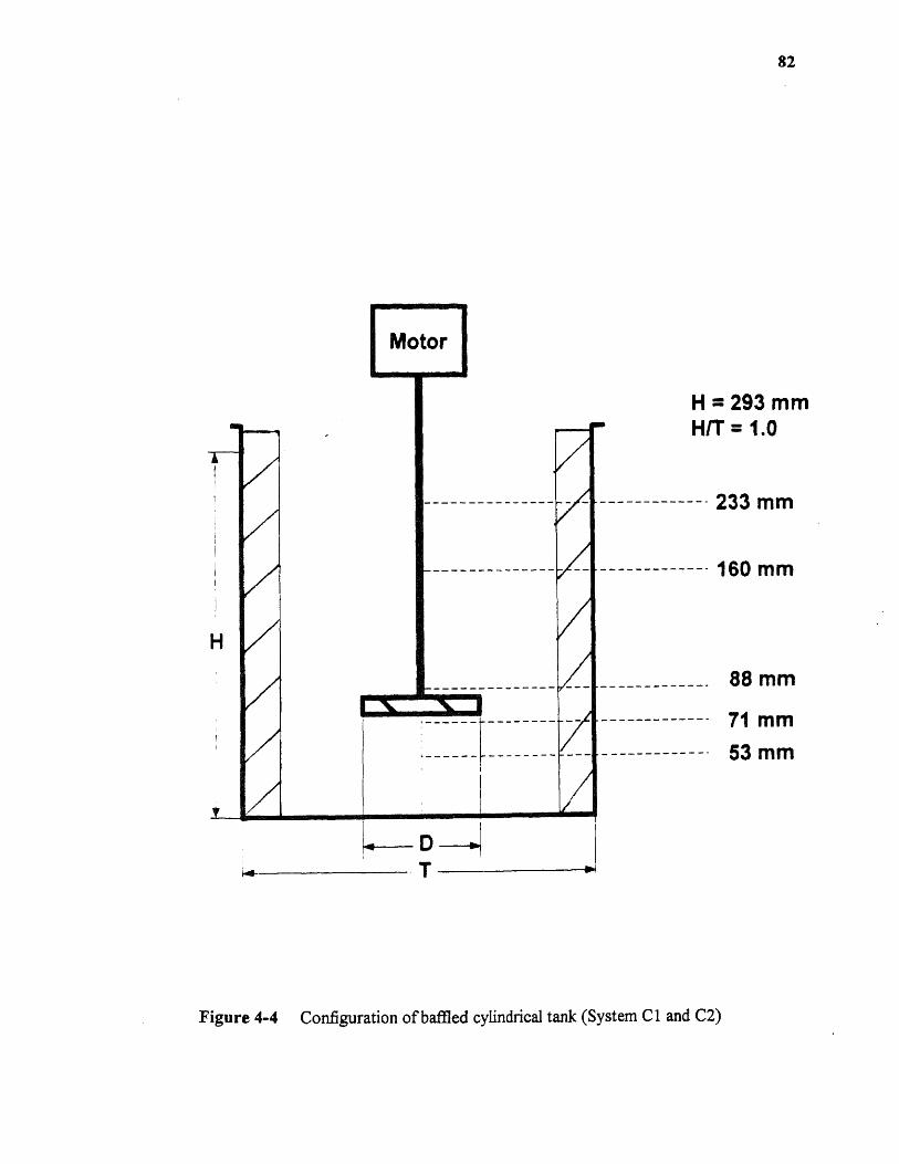
Figure 4-4 Configuration of baffled cylindrical tank (System Cl and C2)

Figure 4-5 Outline of impellers: (a) 6-blade pitched bladed impeller, (b) 2-blade paddle type impeller

Axial and radialvelocity measurement
Traversing Direction ofMixer Apparatus
Impeller
Axial and tangentialvelocity measurement
Traversing Direction ofMixer Apparatus
Figure 4-6 Measurement methods used in determining three velocity components

z rai -Figure 6-1 Experimentally determined (via LDV) dimensionless velocities andturbulent kinetic energies in the impeller region (System A, N = 450 rpm)
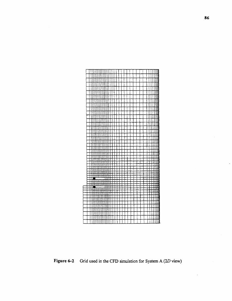
86
Figure 6-2 Grid used in the CFD simulation for System A (2D view)
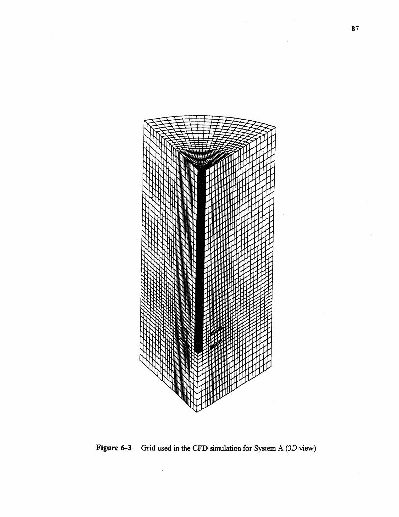
87
Figure 6-3 Grid used in the CFD simulation for System A (3D view)
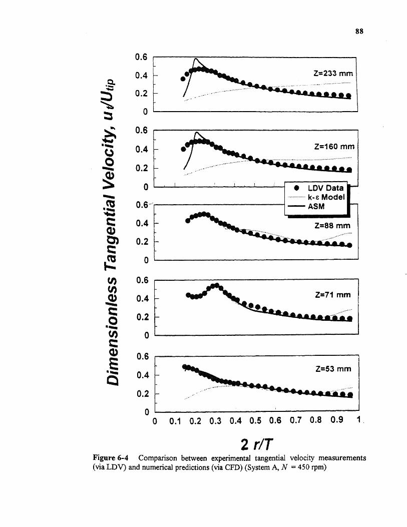
88
Figure 6-4 Comparison between experimental tangential velocity measurements(via LDV) and numerical predictions (via CFD) (System A, N = 450 rpm)
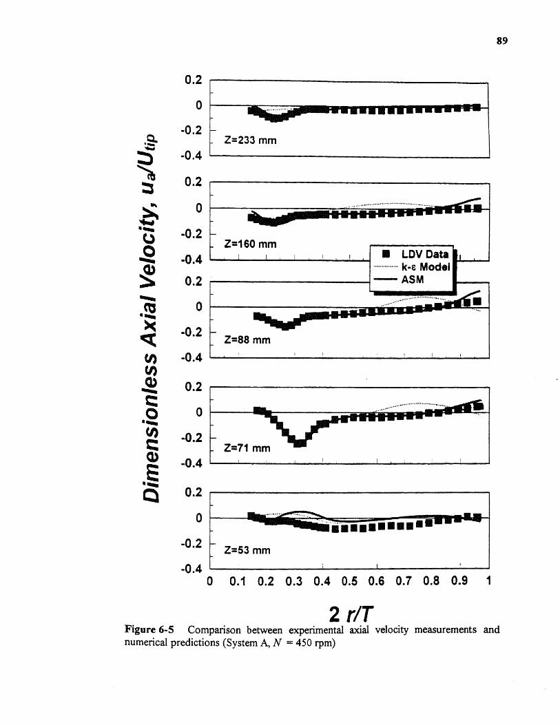
Z=160 mm ■ LDV Data k-c Model- ASM
Z=88 mm
0.2
0
-0.2
-0.4
%*sz 0.2
0
11 140 -0.2
-0.413.)
0.2
CI3
-0.2
tan -0.4ti)
( I) 0.2
2 .0.2
-0.4
89
0
0.1 0.2 0.3 0.4 0.5 0.6 0.7 0.8 0.9 1
riTFigure 6-5 Comparison between experimental axial velocity measurements andnumerical predictions (System A, N = 450 rpm)

0
-0.2 0
90
Z=233 mm
V.V.
0.1 0.2 0.3 0.4 0.5 0.6 0.7 0.8 0.9 1
0.2
0
,Q. -0.2
-0.4
0.2
0
CalS -0.2Z=160 mm
t°173
CO -0.2Z=88 mm
-0.4(1) 0.5
0.3
(i) 0.1
Q) -0.1
0.4
0.2
• LDV Data k-e Mod&
ASM
2 riTFigure 6-6 Comparison between experimental radial velocity measurements andnumerical predictions (System A, N = 450 rpm)
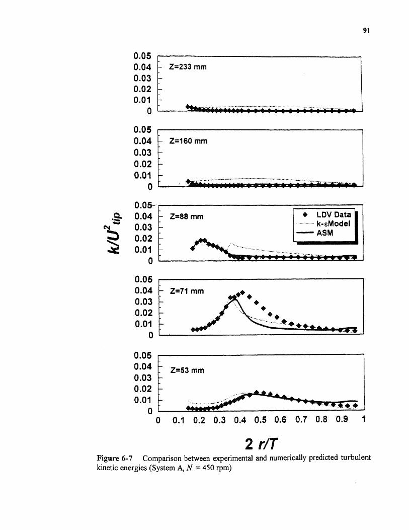
Z=71 mm ♦• • • • •*........ .......
91
0.050.040.030.020.01
0
0.050.040.030.020.01
0
0.05-0. 0.04
1,z 0.030.020.01
0
0.050.040.030.020.01
0
- Z=233 mm
0.050.040.030.020.01
0 0 0.1 0.2 0.3 0.4 0.5 0.6 0.7 0.8 0.9 1
raFigure 6-7 Comparison between experimental and numerically predicted turbulentkinetic energies (System A, N = 450 rpm)

9 2
e,a)
cZ)
0
41-
cu
04°4
ri
. 50
C
srui
0
t)
Cw
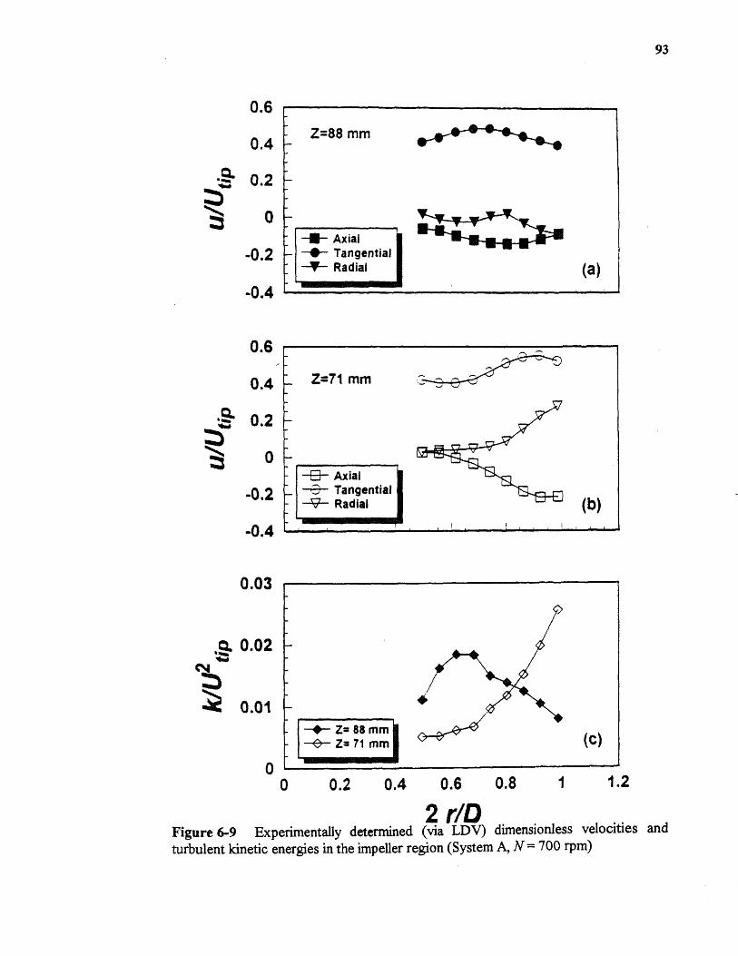
0 0.2 0.4 0.6 0.8 1 1.2
2 ripFigure 6-9 Experimentally determined (via LDV) dimensionless velocities andturbulent kinetic energies in the impeller region (System A, N = 700 rpm)
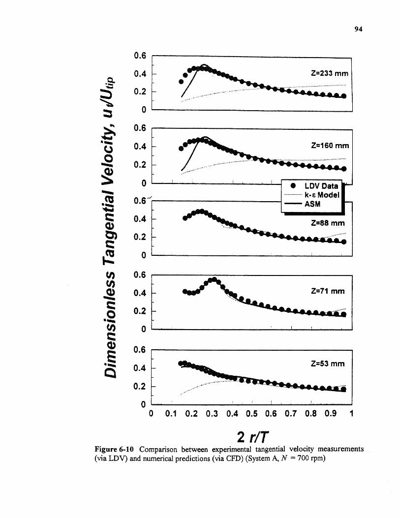
Figure 6-10 Comparison between experimental tangential velocity measurements(via LDV) and numerical predictions (via CFD) (System A, N = 700 rpm)

Figure 6-41 companson between expenmentat dmiti vcit.m.ity —numerical predictions (System A, N = 700 rpm)

Figure 6-12 Comparison between experimental radial velocity measurements andnumerical predictions (System A, N = 700 rpm)

kinetic energies (System A, N = 700 rpm)

❑ Axial0 Tangential7 Radial
0.4
0.2
0
-0.2
00 0.2 0.4 0.6 0.8 1
2 eD1.2 1.4
0.3
0.4
0.2
-0.2
98
Figure 6-14 Experimentally determined (via LDV) dimensionless velocities andturbulent kinetic energies in the impeller region (System B, N = 350 rpm)
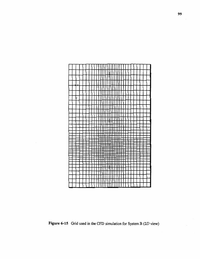
Figure 6-15 Grid used in the CFD simulation for System B (2D view)
99

100
Figure 646 Grid used in the CFD simulation for System B (3D view)

Figure 6-17 Comparison between LDV measurements and CFO predictions:tangential velocity (System B, N = 350 rpm)
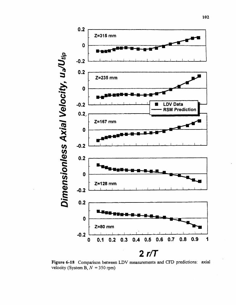
Z=315 mm
■ LDV Data- RSM Prediction
102
0.2
0
-0.2
0.2
0 -0.20.2_,
(1) -0.2(1)0.) 0.2
U)
-0.2
0.2
0- Z=80 mm
-0.20 0.1 0.2 0.3 0.4 0.5 0.6 0.7 0.8 0.9 1
2 riTFigure 6-18 Comparison between LDV measurements and CFD predictions: axialvelocity (System B, N = 350 rpm)

r figure 6-1Y uomparison oetween Loy measurements ana precuutuns.velocity (System B, N = 350 rpm)
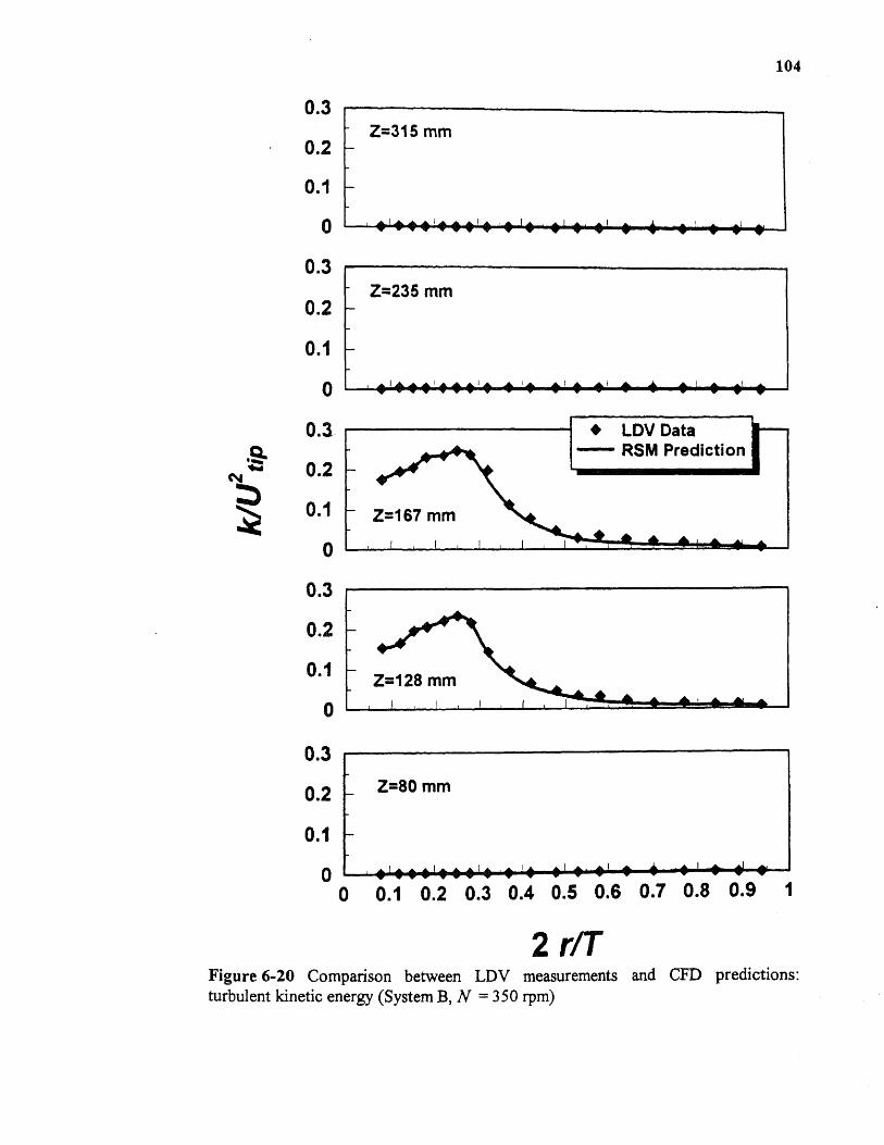
1111
Figure 6-20 Comparison between LDV measurements and CFD predictions:turbulent kinetic energy (System B, N = 350 rpm)
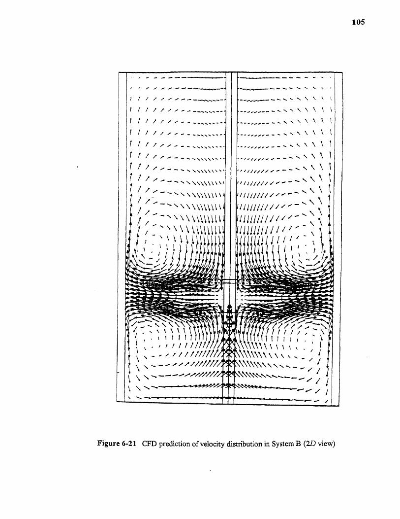
105

Figure 6-22 CFD prediction of velocity distribution in System B (3D view)
106

107
Figure 6-23 CFD prediction of velocity distribution in System B (top view: Z/H =0.18)

108
Figure 6-24 CFD prediction of velocity distribution in System B (top view: Z✓H =0.37)
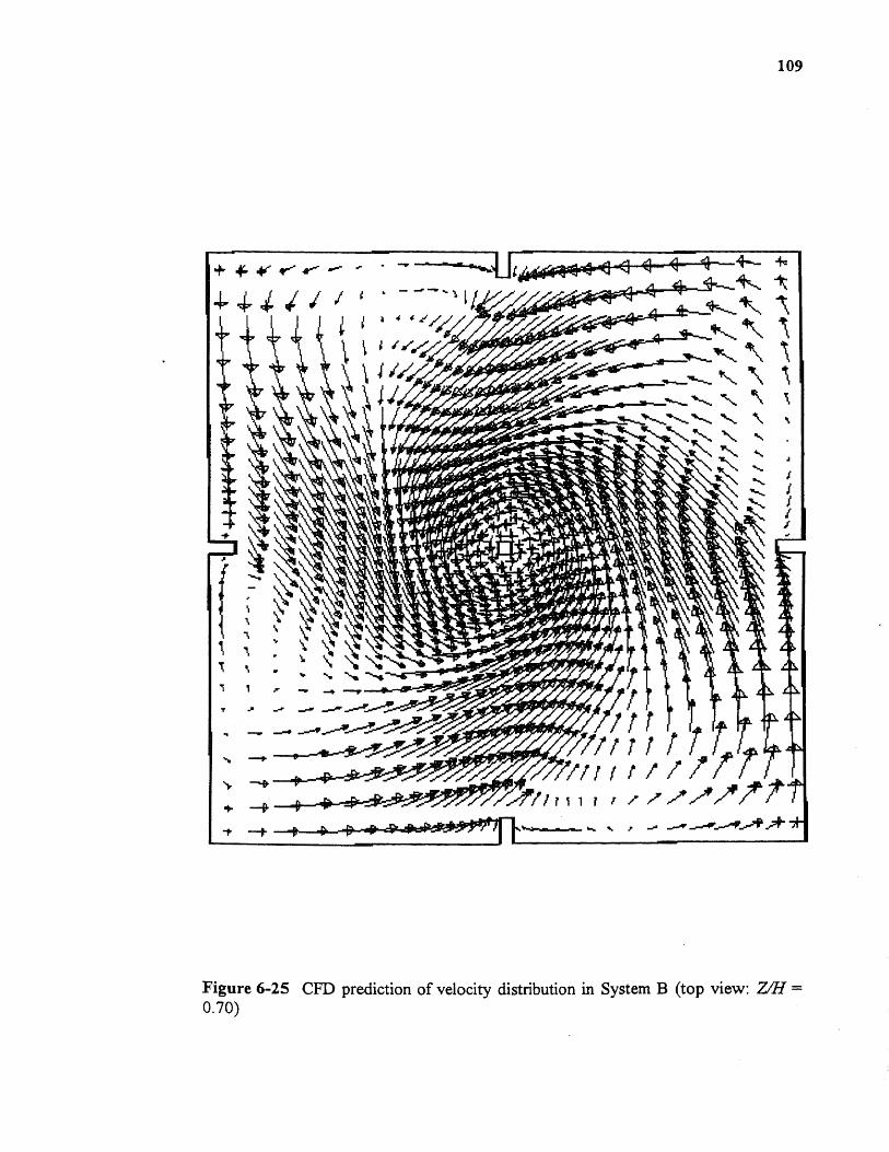
109
Figure 6-25 CFD prediction of velocity distribution in System B (top view: Z/H =0.70)
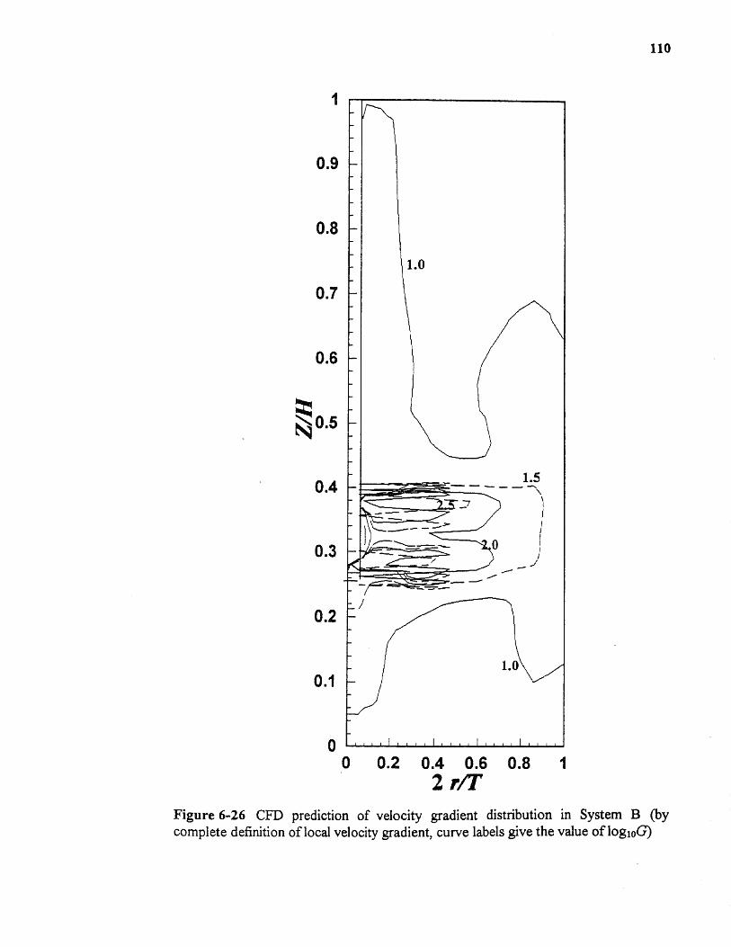
0.9
0.8
110
1.0
0.7
.. ...

Figure 6-27 CFD prediction of velocity gradient distribution in System B (by localenergy dissipation method, curve labels give the value of logioG)
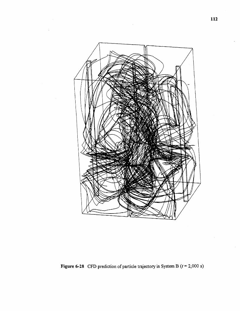
Figure 6-28 CFD prediction of particle trajectory in System B (t = 2,000 s)
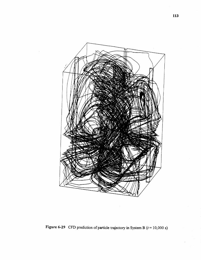
Figure 6-29 CFI) prediction of particle trajectory in System B (t = 10,000 s)
113

Time (s)
Figure 6-30 G value along the particle trajectory in System B
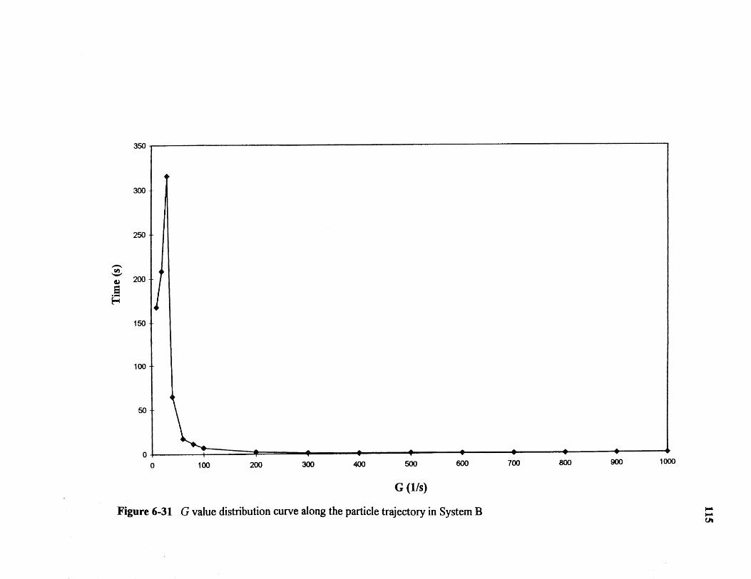
350
250
150
100
•
0 100 200 300 400 500 600 700 800 900 1000
G (1A)
Figure 6-31 G value distribution curve along the particle trajectory in System B

Figure 6-32 Cumulative G value distribution curve along the particle trajectory in System B
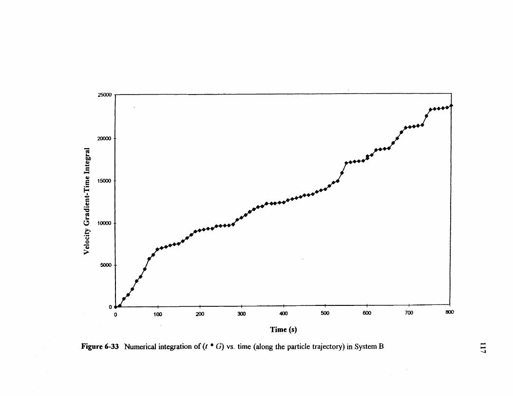
Time (s)
Figure 6-33 Numerical integration of * G) vs. time (along the particle trajectory) in System B

80.0
20.0 )
10.0 -
0.0
70.0 -
60.0 -
50.0 -
40.0 -
30.0 -r
0 100 200 300 400 500 600 700 800
Time (s)
Figure 6-34 Average G value vs. time (along the particle trajectory) in SystemB
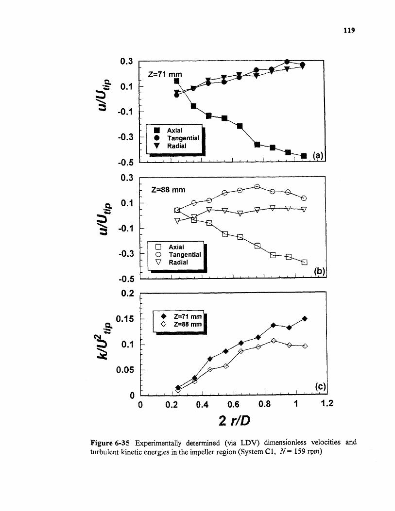
Figure 6-35 Experimentally determined (via LDV) dimensionless velocities andturbulent kinetic energies in the impeller region (System Cl, N= 159 rpm)
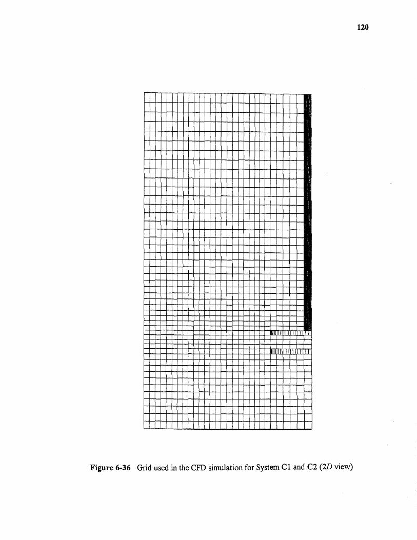
Figure 6-36 Grid used in the CFD simulation for System Cl and C2 (2D view)
120
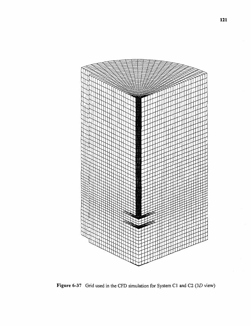
Figure 6-37 Grid used in the CFD simulation for System Cl and C2 (3D view)
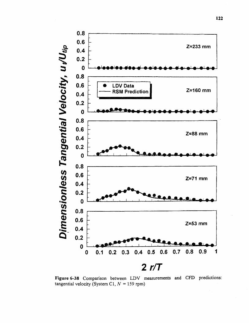
Figure 6-38 Comparison between LDV measurements and utti) precuctions:tangential velocity (System C1 , N = 159 rpm)
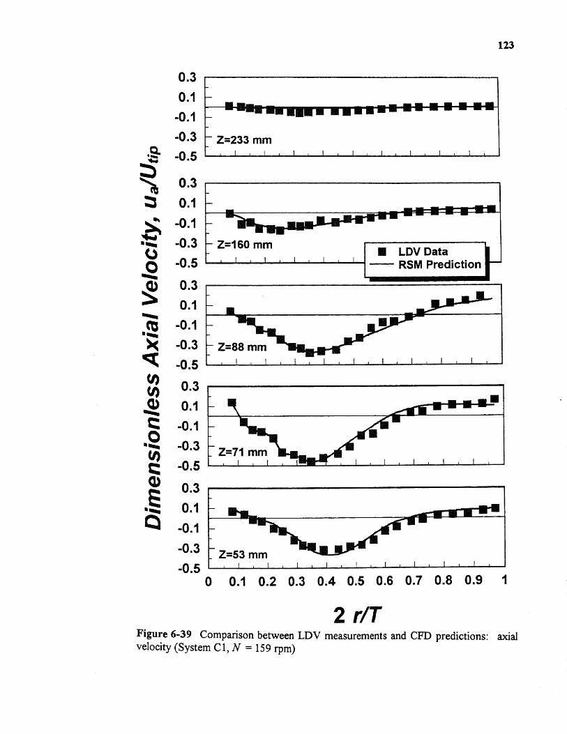
■Figure 6-39 Comparison between LDV measurements and CFD predictions: axialvelocity (System Cl, N = 159 rpm)

Figure 6-40 Comparison between LDV measurements and CFI) predictions: radialvelocity (System Cl, N = 159 rpm)
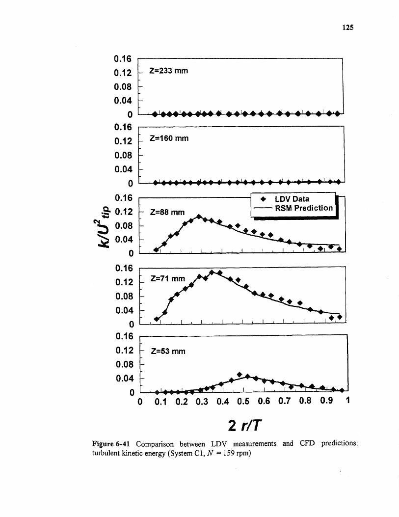
Figure 6-41 Comparison between LDV measurements and CFD predictions:turbulent kinetic energy (System Cl, N = 159 rpm)

Figure 6-42 CFD prediction of velocity distribution in System Cl (2D view)
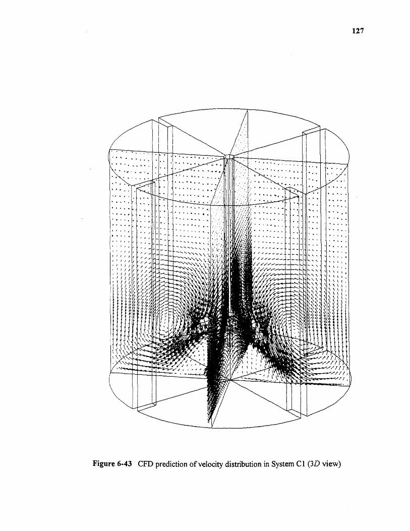
127


Figure 6-45 CFD prediction of particle trajectory in System Cl (1= 2,000 s)
129
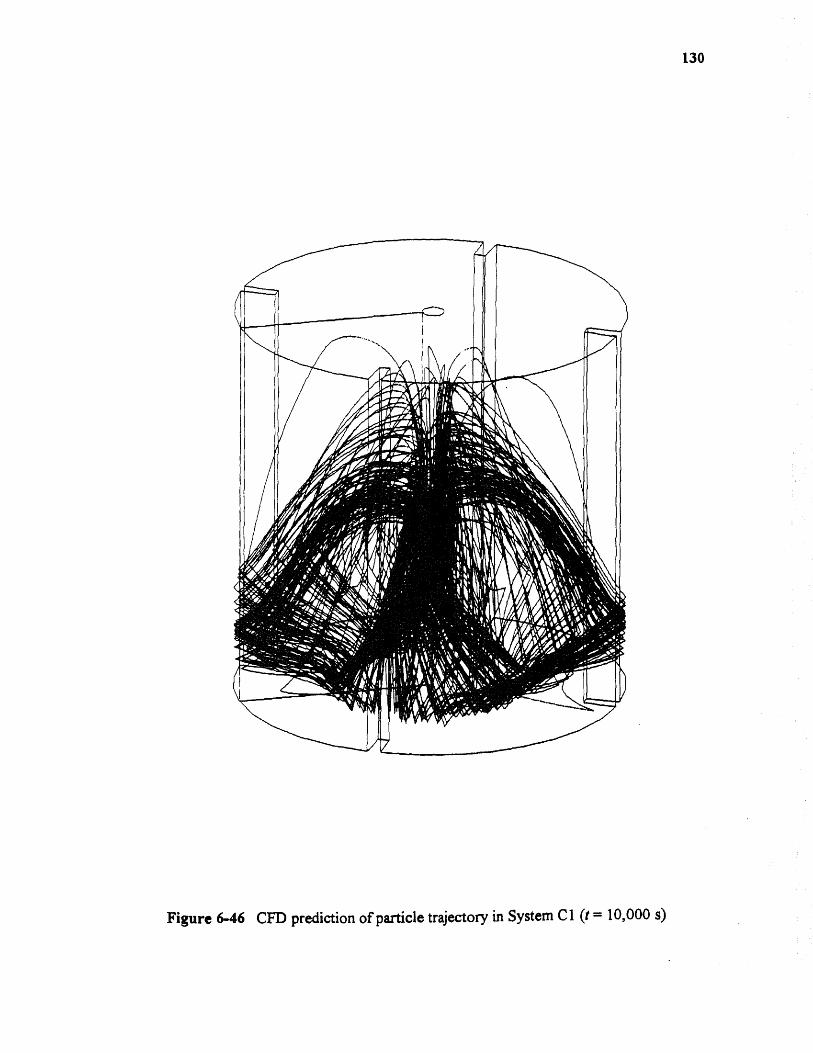
130
Figure 6-46 CFD prediction of particle trajectory in System Cl (t = 10,000 s)

700
•600
Gave byConventional
Method
•
•
100
0 200100 300 400
Time (s)
Figure 6-47 G value along the particle trajectory in system Cl
700600500

400.0
350.0
300.0
250.0
rn
200.0
150.0
100.0
50.0
0.00 100 200 300 400
G (1/s)
Figure 6-48 G value distribution curve along the particle trajectory in system Cl
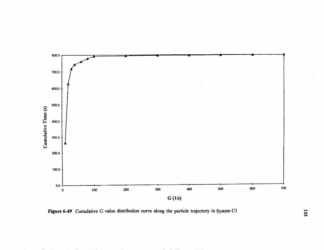
800.0
700.0
600.0
500.0
400.0
200.0
100.0
0.0
Figure 6-49 Cumulative G value distribution curve along the particle trajectory in System Cl

18000
16000
atbD
140001■4
CL)
12000
L....t4 10000
-4"
6000
700 8000 100 200 300 400
500
600
Time (s)
Figure 6-50 Numerical integration of (t * G) vs. time (along the particle trajectory) in System Cl

60.0
0.0 -r-
0 100 200 300 400 500 600 700 800
Time (s)
Figure 6-51 Average G value vs. time (along the particle trajectory) in System Cl
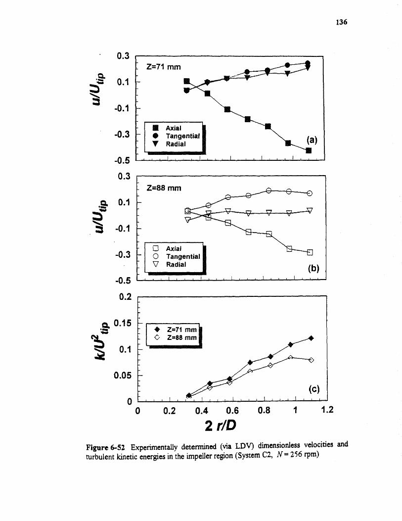
0.2
0.15
0.1
0.05
01.210 0.2 0.4 0.6 0.8
2 rip
0.3
-0.3
-0.5
-0.3
-0.5
• 0.3
0.1
-0.1
136
Figure 6-52 Experimentally determined (via LDV) dimensionless velocities andturbulent kinetic energies in the impeller region (System C2, N= 256 rpm)
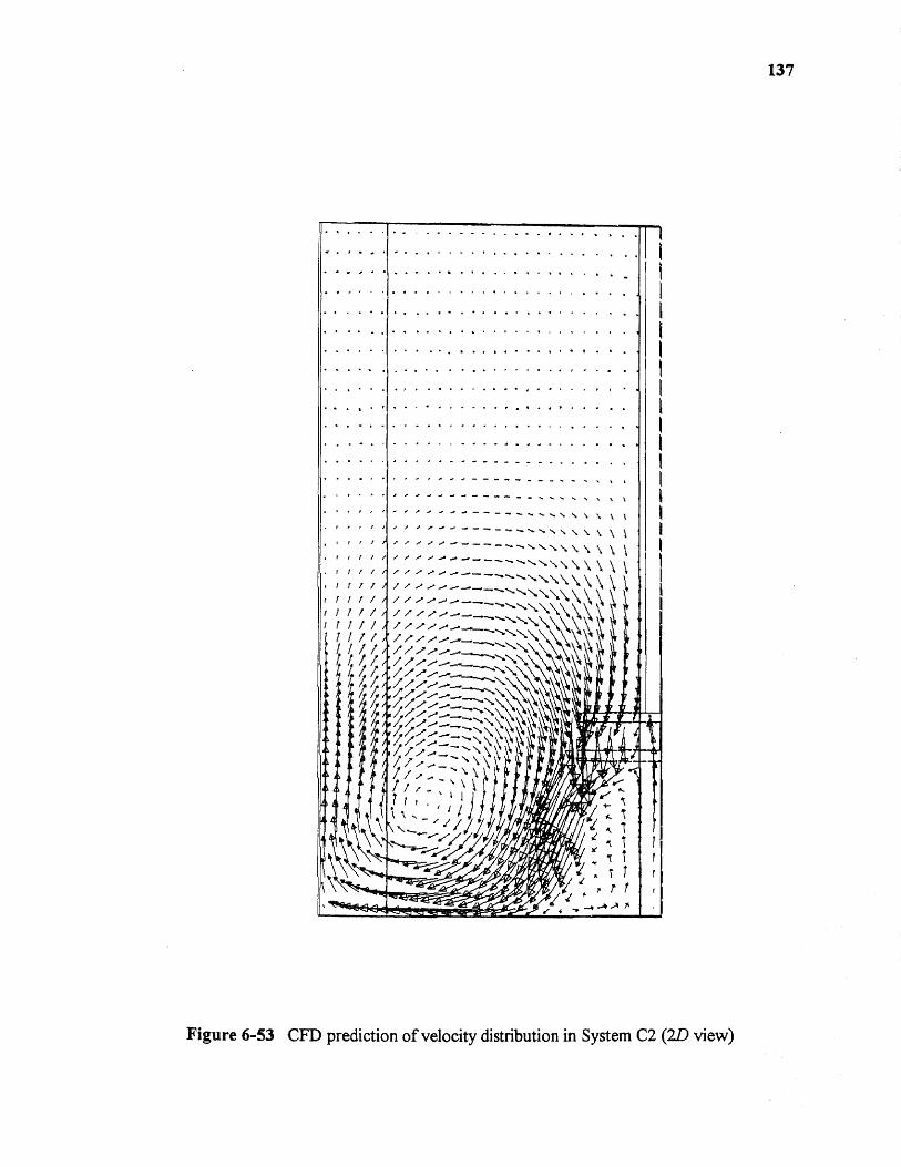
Figure 6-53 CFD prediction of velocity distribution in System C2 (2D view)

138
Figure 6-54 CFD prediction of velocity distribution in System CZ (3D view)

labels give the value of logloG , where G is in s-1)
139

140
Figure 6-56 CFD prediction of particle trajectory in System C2 (t = 2,000 s)

141
Figure 6-57 CFD prediction of particle trajectory in System C2 (t = 10,000 s)

500 700600
1400
1200
1000
0 100 200 300 400
Time (s)
Figure 6-58 G value along the particle trajectory in System C2
•
• • •
• • •••
•
•Gave by
ConventionalMethod••
• • •
•IMMIII M UMW 40111111 11111.11111 •■ 0101.101.
•St
•••••
01111111111 Of ■•••10f =MOM AMON
••
•••
•1111110110•11f
. A ihmahai IL a
•
•• •
•
••
•

350.0
300.0
250.0
200.0
150.0
100.0
50.0
0.00 100 200 300 400 500
600
G (Vs)
Figure 6-59 G value distribution curve along the particle trajectory in System C2

200 300 400 500 600 700 800 900 1000
G (1/s)
Figure 6-60 Cumulative G value distribution curve along the particle trajectory in System C2
1000
800.0
700.0
600.0
500.0
E[..4 400.0
43.)
ad300.0
5
200.0
100.0
0.0

O
tO 250004.)
11:4 200004.0
cgtk 15000
0Ta 1 0000
0 100 200 300 400
500
600
Time (s)
Figure 6-61 Numerical Integration of (t * G) vs. Time (along the Particle Trajectory) in System C2
700
800
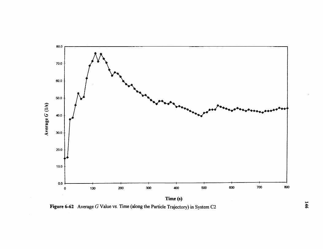
80.0
70.0
60.0
50.0
1-4
40.0taatIJD
aie•'*! 30.0
20.0
10.0
0.00 100 200
Time (s)Figure 6-62 Average G Value vs. Time (along the Particle Trajectory) in System C2

APPENDIX B
PROGRAM CODE FOR THE LOCAL G VALUE CALCULATION
This appendix includes the program code used to perform the calculation of the local
velocity gradient distribution via the complete definition of local velocity gradient
method proposed in this work.
147

LOCAL VELOCITY GRADIENT CALCULATION PROGRAM
' Macro2 Macro
Macro recorded in 04/27/1997 by Changgen Luo
' This Macro is created to calculated the local velocity gradient
This is a mcaro programmed in MS Excel 5.0, working together with' data sheets imported from FLUENT V4.4,I Following imported data sheets are included in this Excel Workbook:
xp: x position (cartesian coordinates)in each cell center,yp: y position (cartesian coordinates)in each cell center,zp: z position (cartesian coordinates)in each cell center,uv: U velocity in each cellvv: V velocity in each cellwv: W velocity in each cellzp: axial position (cylindrical coordinates)in each cell center,tp: tangential position (cylindrical coordinates)in each cell center,rp: radial position (cylindrical coordinates)in each cell center,zv: velocity in axial dircetion in each cellrv: velocity in radial direction in each celltv: velocity in tangential in each celleff:effective viscosity in each cell
The results of local velocity gradient will be put in worksheet"Gvalue" in the same workbook
Sub Macro()Dim t, counter, Rownum, Colnum, GRownum, GColnum As IntegerDim i, j, k, Maxi, Maxj, Maxk, Cood As IntegerDim xl, x0, yl, yO, zl, zO, uvl, uvO, vvl, wO, wvl, wv0 As SingleDim dx, dy, dz, dux, duy, duz As SingleDim Gxx, Gyy, Gzz, Gxy, Gyx, Gyz, Gzy, Gxz, Gzx As SingleDim Gl, G2, G As SingleDim zvl, zv0, rvl, rvO, tvl, tv0 As SingleDim duz, dur, dut, dutr As SingleDim Gtt, Gzz, Grr, Grt, Gtr, Gtz, Gzt, Grz, Gzr As Single
VISCOSITY = 0.001
Cood = Val(InputBox("Please enter 1 if it is cartesian coordinate, or 0 if cylindrical","Which Coordinate System", 1))
Maxi = Val(InputBox("Please enter the number of i", "i Value Entry", 5))
148

Maxj = Val(InputBox("Please enter the number of j", "j Value Entry", 5))Maxk = Val(InputBox("Please enter the number of k", "k Value Entry", 5))
If Cood = 1 Then
'This part is for the local velocity gradient calculation' in cartesian coordiate.
For k = 1 To MaxkFor j = 1 To Maxj
For i = 1 To Maxi
If ((i Mod 10) = 0) ThenRownum = (((k - 1) * 156 + 8) + (35 - j) + (((i \ 10) - 1) * 38))Colnum = 11ElseRownum = (((k - 1) * 156 + 8) + (35 - j) + ((i \ 10) * 38))Colnum = ((i Mod 10) + 1)'Where 156 is the number of rows for each k value block in "zx" sheet
8 is the number of rows before the first x position value(35 - j) indicates that x position values were listed
in reverse sequence(i mod 10) gives the reminder of this division(i \ 10) gives the integer of this division((i \ 10) * 38) indicates for every 10 I values we have 38 rowsthe position values were listed in column 2 to 11
End IfGRownum = RownumGColnum = Colnumx0 = Worksheet("'xp").Cells(Rownum, Colnum).Valuey0 = Worksheet(""yp").Cells(Rownum, Colnum).Valuez0 = Worksheet("zp").Cells(Rownum, Colnum).Valueuv0 = Worksheet("uv").Cells(Rownum, Colnum).Valuew0 = Worksheet("w").Cells(Rownum, Colnum).Valuewv0 = Worksheet("wv").Cells(Rownum, Colnum).Valueeffv = Worksheet('"eff").Cells(Rownum, Colnum).Value
k = k + 1If ((i Mod 10) = 0) ThenRownum = (((k - 1) * 156 + 8) + (35 - j) + (((i \ 10) - 1) * 38))Colnum = 11ElseRownum = (((k - 1) * 156 + 8) + (35 - j) + ((i \ 10) * 38))Colnum = ((i Mod 10) + 1)End If
149
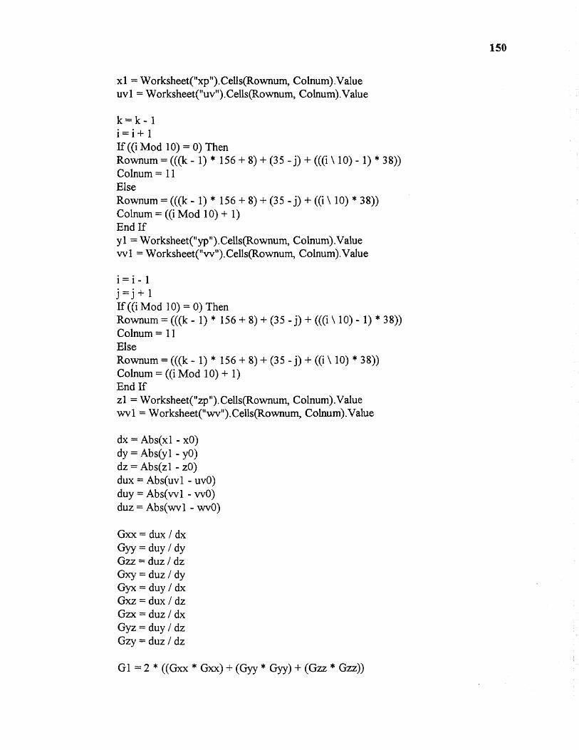
xl = Worksheet("xp").Cells(Rownum, Colnum).Valueuv1 = Worksheet("uv").Cells(Rownum, Colnum).Value
k = k 1i=i+1If ((i Mod 10) = 0) ThenRownum = (((k - 1) * 156 + 8) + (35 - j) + (((i 1 10) - 1) * 38))Colnum = 11ElseRownum = (((k - 1) * 156 + 8) + (35 - j) + ((i \ 10) * 38))Colnum = ((i Mod 10) + 1)End Ify1 = Worksheet("yp").Cells(Rownum, Colnum).Valuevvl = Worksheet("vv").Cells(Rownum, Colnum).Value
i = - 1j = j + 1If ((i Mod 10) = 0) ThenRownum = (((k 1) * 156 + 8) + (35 - j) + (((i \ 10) - 1) * 38))Colnum = 11ElseRownum = (((k - 1) * 156 + 8) + (35 - j) + ((i \ 10) * 38))Colnum = ((i Mod 10) + 1)End Ifzl = Worksheet("zp").Cells(Rownum, Colnum).Valuewvl = Worksheet("wv").Cells(Rownum, Colnum).Value
dx = Abs(xl - x0)dy = Abs(y1 yO)dz = Abs(zl - z0)dux = Abs(uvl - uvO)duy = Abs(vvl vv0)duz = Abs(wvl - wv0)
Gxx = dux / dxGyy = duy / dyGzz = duz / dzGxy = duz / dyGyx = duy / dxGx2 = dux / dzGzx = duz / dxGyz = duy / dzGzy = duz / dz
G1 = 2 * ((Gxx * Gxx) + (Gyy * Gyy) + (Gzz * Gzz))
150
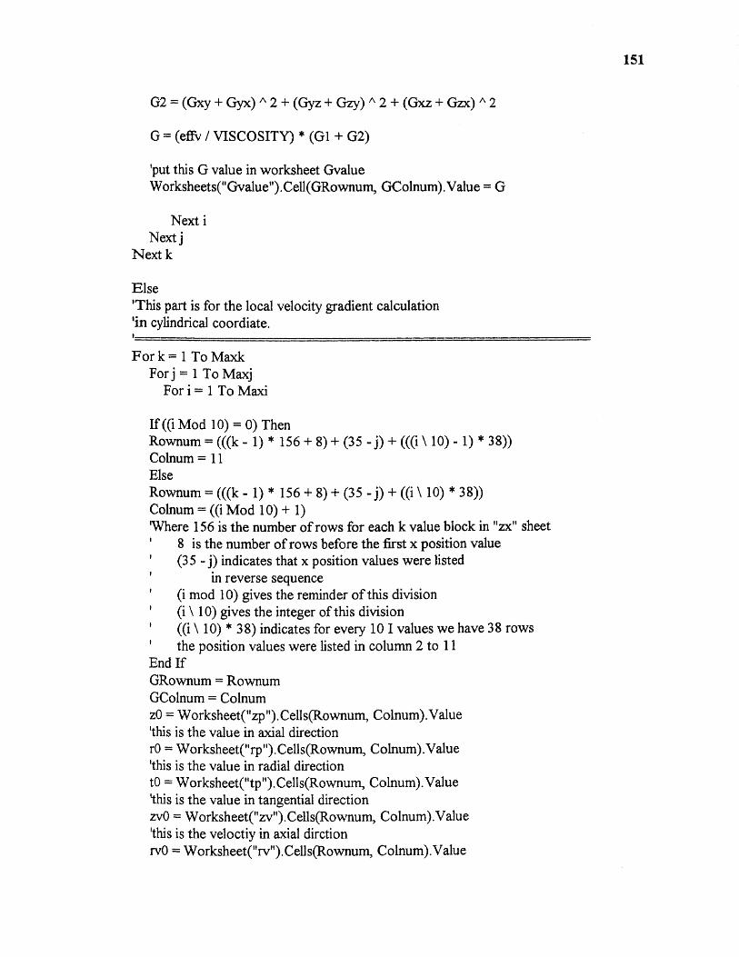
G2 = (Gxy + Gyx) A 2 + (Cryz + Gzy) A 2 + (Gxz + Gzx) A 2
G = (dry / VISCOSITY) * (G1 + G2)
'put this G value in worksheet GvalueWorksheets("Gvalue").Cell(GRownum, GColnum).Value = G
Next iNext j
Next k
Else'This part is for the local velocity gradient calculation'in cylindrical coordiate.
For k = 1 To MaxkFor j = 1 To Maxj
For i = 1 To Maxi
If ((i Mod 10) = 0) ThenRownum = (((k - 1) * 156 + 8) + (35 - j) + (((i \ 10) - 1) * 38))Colnum = 11ElseRownum = (((k - 1) * 156 + 8) + (35 - j) + ((i 1 10) * 38))Colnum = ((i Mod 10) + 1)'Where 156 is the number of rows for each k value block in "zx" sheet
8 is the number of rows before the first x position value(35 j) indicates that x position values were listed
in reverse sequence(i mod 10) gives the reminder of this division(i \ 10) gives the integer of this division((i \ 10) * 38) indicates for every 10I values we have 38 rowsthe position values were listed in column 2 to 11
End IfGRownum = RownumGColnum = Colnumz0 = Worksheet("zp").Cells(Rownum, Colnum).Value'this is the value in axial directionr0 = Worksheet("rp").Cells(Rownum, Colnum).Value'this is the value in radial directiontO = Worksheet("tp").Cells(Rownum, Colnum).Value'this is the value in tangential directionzv0 = Worksheet("zv").Cells(Rownum, Colnum).Value'this is the veloctiy in axial dirctionrv0 = Worksheet("rv").Cells(Rownum, Colnum).Value
151

'this is the veloctiy in radial dirctiontv0 = Worksheet("tv").Cells(Rownum, Colnum).Value'this is the veloctiy in tangential dirctioneffv = Worksheet("eff').Cells(Rownum, Colnum).Value
k = k + 1If ((i Mod 10) = 0) ThenRownum = (((k - 1) * 156 + 8) + (35 j) + (((i \ 10) - 1) * 38))Colnum = 11ElseRownum = (((k - 1) * 156 + 8) + (35 j) + ((i 10) * 38))Colnum = ((i Mod 10) + 1)End Ifzl = Worksheet("zp").Cells(Rownum, Colnum).Valuezvl = Worksheet("zv").Cells(Rownum, Colnum).Value
k = k 1i = i + 1If ((i Mod 10) = 0) ThenRownum = (((k - 1) * 156 + 8) + (35 - j) + (((i \ 10) - 1) * 38))Colnum = 11ElseRownum = (((k - 1) * 156 + 8) + (35 j) + ((i \ 10) * 38))Colnum = ((i Mod 10) + 1)End Ifrl = Worksheet("rp").Cells(Rownum, Colnum).Valuervl = Worksheet("rv").Cells(Rownum, Colnum).Value
i =i- 1j = j + 1If ((i Mod 10) = 0) ThenRownum = (((k - 1) * 156 + 8) + (35 - j) + (((i \ 10) - 1) * 38))Colnum = 11ElseRownum = (((k - 1) * 156 + 8) + (35 - j) + ((i \ 10) * 38))Colnum = ((i Mod 10) + 1)End Iftl = Worksheet("tp").Cells(Rownum, Colnum).Valuetv1 = Worksheet("tv").Cells(Rownum, Colnum).Value
dz = Abs(zl - z0)dr = Abs(r1 - r0)dt = Abs(tl - tO) 'refer to theta
duz = Abs(zvl - zvO)
152
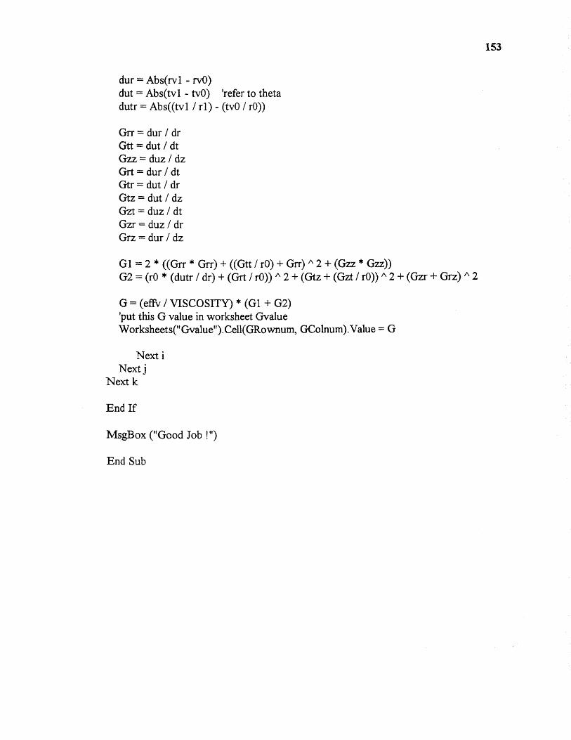
dur = Abs(rvl rv0)dut = Abs(tvl - tv0) 'refer to thetadutr = Abs((tvl I r1) - (tv0 / r0))
Grr = dur / drGtt = dut / dtGzz = duz / dzGrt = dur / dtGtr = dut / drGtz = dut / dzGzt = duz / dtCrzr = duz / drGrz = dur / dz
G1 =2 * ((Grr * Grr) + ((Gtt / r0) + Grr) A 2 + (Gzz * Gzz))G2 = * (dutr / dr) + (Grt / r0)) A 2 + (Gtz + (Gzt / r0)) A 2 + (Gzx + Grz) A 2
G = (effv / VISCOSITY) * (G1 + G2)'put this G value in worksheet GvalueWorksheets(" Gvalue"). GColnum).Value = G
Next iNext j
Next k
End If
MsgBox ("Good Job !")
End Sub
153
APPENDIX C
PROGRAM CODE FOR NEW PARAMETER CALCULATION
This appendix includes the program code used to perform the calculation of the local
velocity gradient distribution, velocity gradient distribution along the particle trajectory,
velocity gradient-time integral from FLUENT output data.
154
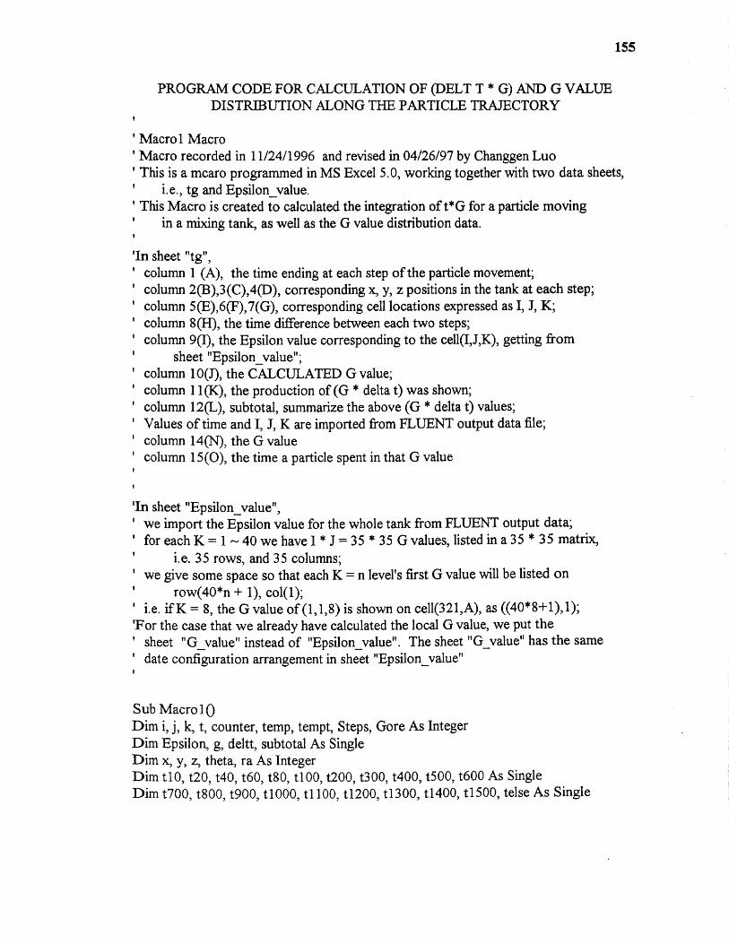
155
PROGRAM CODE FOR CALCULATION OF (DELT T * G) AND G VALUEDISTRIBUTION ALONG THE PARTICLE TRAJECTORY
Macro 1 MacroMacro recorded in 11/24/1996 and revised in 04/26/97 by Changgen Luo
'This is a mcaro programmed in MS Excel 5.0, working together with two data sheets,i.e., tg and Epsilon_value.
This Macro is created to calculated the integration of t*G for a particle movingin a mixing tank, as well as the G value distribution data.
'In sheet "tg",column 1 (A), the time ending at each step of the particle movement;column 2(B),3(C),4(D), corresponding x, y, z positions in the tank at each step;column 5(E),6(F),7(G), corresponding cell locations expressed as I, J, K;column 8(H), the time difference between each two steps;column 9(I), the Epsilon value corresponding to the cell(I,J,K), getting from
sheet "Epsilon_value";column 10(J), the CALCULATED G value;column 11(K), the production of (G * delta t) was shown;column 12(L), subtotal, summarize the above (G * delta t) values;Values of time and I, J, K are imported from FLUENT output data file;column 14(N), the G valuecolumn 15(0), the time a particle spent in that G value
' In sheet "Epsilon_value",we import the Epsilon value for the whole tank from FLUENT output data;for each K = 1 — 40 we have I * J = 35 * 35 G values, listed in a 35 * 35 matrix,
i.e. 35 rows, and 35 columns;we give some space so that each K = n level's first G value will be listed on
row(40*n + 1), col(1);i.e. if K = 8, the G value of (1,1,8) is shown on cell(321,A), as ((40*8+1) 1);
'For the case that we already have calculated the local G value, we put thesheet "G_value" instead of "Epsilon_value". The sheet "G_value" has the samedate configuration arrangement in sheet "Epsilon_value"
Sub Macro 10Dim i, j, k, t, counter, temp, tempt, Steps, Gore As IntegerDim Epsilon, g, deltt, subtotal As SingleDim x, y, z, theta, ra As IntegerDim t10, t20, t40, t60, t80, t100, t200, t300, t400, t500, t600 As SingleDim t700, t800, t900, t1000, t1100, t1200, t1300, t1400, t1500, telse As Single
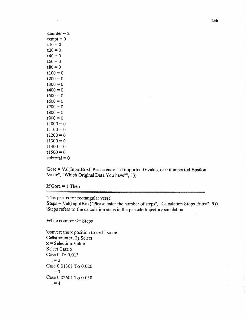
156
counter = 2tempt = 0t10=0t20 = 0t40 = 0t60 = 0t80 = 0t100 = 0t200 = 0t300 = 0t400 = 0t500 = 0t600 = 0t700 = 0t800 = 0t900 = 0t1000 = 0t1100 = 011200 = 011300 = 0t1400 = 0t1500 = 0subtotal = 0
Gore = Val(InputBox("Please enter 1 if imported G value, or 0 if imported EpsilonValue", "Which Original Data You have?", 1))
If Gore = 1 Then
'This part is for rectangular vesselSteps = Val(InputBox("Please enter the number of steps", "Calculation Steps Entry", 5))'Steps refers to the calculation steps in the particle trajectory simulation
While counter <= Steps
'convert the x position to cell I valueCells(counter, 2).Selectx = Selection. ValueSelect Case xCase 0 To 0.013
i = 2Case 0.01301 To 0.026
i = 3Case 0.02601 To 0.038
i = 4
157
i = 27Case 0.21701 To 0.227
i = 28Case 0.22701 To 0.238
i = 29Case 0.23801 To 0.25
i = 30Case 0.25001 To 0.262
i = 31Case 0.26201 To 0.274
i = 32Case 0.27401 To 0.287
i = 33Case 0.28701 To 0.3
i = 34Case Else
MsgBox ("please check the x position") 'check if x value is in the correct rangeDebug.Print counter; x; y; z 'Display the position in the Debug Window
End Select
'convert the y position to cell J valueCells(counter, 3). Selecty = Selection. ValueSelect Case yCase 0 To 0.013
j = 2Case 0.01301 To 0.026
3Case 0.02601 To 0.038
j = 4Case 0.03801 To 0.05
5Case 0.05001 To 0.062
j = 6Case 0.06201 To 0.073
7Case 0.07301 To 0.083
8Case 0.08301 To 0.092
9Case 0.09201 To 0.1
j = 10Case 0.10001 To 0.108
j = 11
158

Case 0.10801 To 0.115= 12
Case 0.11501 To 0.121j = 13
Case 0.12101 To 0.127j= 14
Case 0.12701 To 0.134j = 15
Case 0.13401 To 0.141j = 16
Case 0.14101 To 0.147j = 17
Case 0.14701 To 0.153j = 18
Case 0.15301 To 0.16j = 19
Case 0.16001 To 0.166j = 20
Case 0.16601 To 0.172j = 21
Case 0.17201 To 0.179j = 22
Case 0.17901 To 0.185j = 23
Case 0.18501 To 0.192j = 24
Case 0.19201 To 0.2j = 25
Case 0.20001 To 0.208j =26
Case 0.20801 To 0.217j = 27
Case 0.21701 To 0.227j =28
Case 0.22701 To 0.238j = 29
Case 0.23801 To 0.25j = 30
Case 0.25001 To 0.262j = 31
Case 0.26201 To 0.274j = 32
Case 0.27401 To 0.287j = 33
Case 0.28701 To 0.3
159
j = 34Case Else
MsgBox ("please check the y position") 'check if y value is in the correct rangeDebug.Print counter; x; y; z 'Display the position in the Debug Window
End Select
'convert the z position to cell K valueCells(counter, 4). Selectz = Selection.ValueSelect Case zCase 0 To 0.016
k = 2Case 0.01601 To 0.035
k = 3Case 0.03501 To 0.046
k = 4Case 0.04601 To 0.06
k = 5Case 0.06001 To 0.073
k = 6Case 0.07301 To 0.084
k = 7Case 0.08401 To 0.094
k = 8Case 0.09401 To 0.103
k = 9Case 0.10301 To 0.11
k= 10Case 0.11001 To 0.116
k= 11Case 0.11601 To 0.123
k= 12Case 0.12301 To 0.129
k= 13Case 0.12901 To 0.135
k= 14Case 0.13501 To 0.142
k= 15Case 0.14201 To 0.148
k= 16Case 0.14801 To 0.155
k= 17Case 0.15501 To 0.161
k= 18Case 0.16101 To 0.167
160
.■•••

'calculate the G value, put in column 10

163
Cells(counter, 10).Value = 1000 * ((Epsilon) A 0.5)'Cells(counter, 10).Value = Epsilon * 2 'This line just for testingCells(counter, 10). Selectg = Selection.Value
Else1 1-11111111111111111114-111111111111111111111
'This part is for cylindrical vessel
Steps = Val(InputBox("Please enter the number of steps", "Calculation Steps Entry", 5))'Steps refers to the calculation steps in the particle trajectory simulation
While counter <= Steps
'convert the tangential position to cell I valueCells(counter, 2). Selecttheta = Selection.ValueSelect Case thetaCase 0 To 0.121
i = 2Case 0.12101 To 0.181
i = 3Case 0.18101 To 0.242
i = 4Case 0.24201 To 0.302
i = 5Case 0.30201 To 0.362
i = 6Case 0.36201 To 0.423
i = 7Case 0.42301 To 0.483
i = 8Case 0.48301 To 0.543
i = 9Case 0.54301 To 0.604
i= 10Case 0.60401 To 0.664
i = 11Case 0.66401 To 0.725
= 12Case 0.72501 To 0.785
i= 13Case 0.78501 To 0.845
i= 14Case 0.84501 To 0.906

i= 15Case 0.90601 To 0.966
i = 16Case 0.96601 To 0.103
i = 17Case 0.10301 To 0.109
i= 18Case 0.10901 To 0.115
i = 19Case 0.11501 To 0.121
i = 20Case 0.12101 To 0.127
i = 21Case 0.12701 To 0.133
i = 22Case 0.13301 To 0.139
i = 23Case 0.13901 To 0.145
i = 24Case 0.14501 To 0.151
i = 25Case 0.15101 To 0.157
i = 26Case Else
MsgBox ("please check the x position") 'check if tangential value is in the correctrange
Debug.Print counter; x; y; z 'Display the position in the Debug WindowEnd Select
'convert the radial position to cell J valueCells(counter, 3). Selectra = Selection. ValueSelect Case raCase 0 To 0.0069
j = 2Case 0.0069 To 0.0125
3Case 0.012501 To 0.0186
j = 4Case 0.018601 To 0.0245
5Case 0.024501 To 0.0302
j = 6Case 0.030201 To 0.0357
164

il / P.

166
Case 0.14201 To 0.147j = 30
Case ElseMsgBox ("please check the y position") 'check if radial value is in the correct rangeDebug.Print counter; x; y; z 'Display the position in the Debug Window
End Select
'convert the z position to cell K valueCells(counter, 4).Selectz = Selection.ValueSelect Case zCase 0 To 0.0066
k = 2Case 0.006601 To 0.0132
k = 3Case 0.013201 To 0.0196
k = 4Case 0.019601 To 0.0261
k = 5Case 0.026101 To 0.0323
k = 6Case 0.032301 To 0.0383
k = 7Case 0.038301 To 0.0443
k = 8Case 0.044301 To 0.0499
k = 9Case 0.049901 To 0.0553
k = 10Case 0.055301 To 0.0605
k= 11Case 0.060501 To 0.0653
k = 12Case 0.065301 To 0.07
k = 13Case 0.070001 To 0.074
k = 14Case 0.07401 To 0.078
k= 15Case 0.07801 To 0.082
k = 16Case 0.08201 To 0.086
k= 17Case 0.08601 To 0.09
k= 18

Case 0.09001 To 0.094k= 19
Case 0.09401 To 0.0988k = 20
Case 0.098801 To 0.1035k = 21
Case 0.103501 To 0.1084k = 22
Case 0.108401 To 0.1134k = 23
Case 0.113401 To 0.1186k = 24
Case 0.118601 To 0.124k = 25
Case 0.12401 To 0.129k = 26
Case 0.12901 To 0.135k = 27
Case 0.13501 To 0.142k = 28
Case 0.14201 To 0.148k = 29
Case 0.14801 To 0.154k= 30
Case 0.15401 To 0.161k = 31
Case 0.16101 To 0.167k = 32
Case 0.16701 To 0.174k = 33
Case 0.17401 To 0.181k = 34
Case 0.18101 To 0.188k = 35
Case 0.18801 To 0.196k = 36
Case 0.19601 To 0.203k = 37
Case 0.20301 To 0.211k= 38
Case 0.21101 To 0.219k= 39
Case 0.21901 To 0.227k = 40
Case 0.22701 To 0.235
167
k = 41Case 0.23501 To 0.243
k = 42Case 0.24301 To 0.251
k = 43Case 0.25101 To 0.259
k = 44Case 0.25901 To 0.268
k = 45Case 0.26801 To 0.276
k = 46Case 0.27601 To 0.285
k = 47Case 0.28501 To 0.293
k = 48Case Else
MsgBox ("please check the z position") 'check if z value is in the correct rangeDebug.Print counter; x; y; z 'Display the position in the Debug Window
End Select
'put I value in column 5Cells(counter, 5).Value = i
'put J value in column 6Cells(counter, 6).Value = j
'put K value in column 7Cells(counter, 7).Value = k
'copy the G value of cell(i,j,k) from sheet "G value"Worksheets("Gvalue").SelectIf ((i Mod 10) = 0) ThenCells((((k - 1) * 156 + 8) + (35 - j) + (((i \ 10) - 1) * 38)), 11).SelectElseCells((((k - 1) * 156 + 8) + (35 j) + ((i \ 10) * 38)), ((i Mod 10) + 1)).Select'Where 156 is the number of rows for each k value block in "Epsilon value" sheet
8 is the number of rows before the first G value(35 - j) refers to G values were listed on reverse sequence(i mod 10) gives the reminder of this division(i \ 10) gives the integer of this division((i \ 10) * 38) indicates for each 10 I values we have 38 rows
End Iftemp = Selection.Value
168
4 IA

Case 700 To 800t800 = t800 + deltt
Case 800 To 900t900 = t900 + deltt
Case 900 To 1000t1000 = t1000 + deltt
Case 1000 To 1100t 1100 = t 1100 + deltt
Case 1100 To 1200t1200 = t1200 + deltt
Case 1200 To 1300t1300 = t1300 + deltt
Case 1300 To 1400t1400 = t1400 + deltt
Case 1400 To 1500t1500 = t1500 + deltt
Case Elsetelse = telse + deltt'MsgBox ("G value out of range") 'check if G value is in the correct rangeDebug.Print counter; x; y; z, g 'Display the position in the Debug Window
End Select
counter = counter + 1
'Output the distribution results'put them in column 14 (G value), 15(time spent in the G value)Cells(2, 14).Value = 10Cells(2, 15).Value = t10
Cells(3, 14).Value = 20Cells(3, 15).Value = t20
Cells(4, 14).Value = 40Cells(4, 15).Value = t40
Cells(5, 14).Value = 60Cells(5, 15).Value = t60
Cells(6, 14).Value = 80Cells(6, 15).Value = t80
Cells(7, 14).Value = 100Cells(7, 15).Value = t100
Cells(8, 14).Value = 200
170

171
Cells(23, 15).Value = t
WendMsgBox ("Good Job !")'End of program
End Sub
172

REFERENCES
Amirtharajah, A. and Mills, K. M., "Rapid Mix Design for Mechanisms of AlumCoagulation", J. AWWA, 74: 210-216 (1982).
Amirtharajah, a. and Trusler, S. L., "Destabilization of Particles by Turbulent RapidMixing", J. Environ. Eng., 112: 1085-1108 (1987).
Argaman, Y., and Kaufman, W. J., "Turbulence and Flocculation", Journal of theSanitary Engineering Division, ASCE, 96(2): 223 -241 (1970).
Armenante, P. M. and Chou, C. C., "Experimental LDV Measurement and NumericalCFD Determination of the Fluid Velocity Distribution in an Unbaffled MixingVessel", AIChE Symp. Ser., 90 (299): 33-42 (1994a).
Armenante P. M., Chou, C. C. and Hemrajani, R. R., "Comparison of Experimental andNumerical Fluid Velocity Distribution Profiles in an Unbaffled Mixing VesselProvided with a Pitched-Blade Turbine", Proc. 8th Europ. Conf. Mixing (I. Chem.Eng. Symp. Ser. No. 136), Cambridge, U.K, 21: 349-356, September (1994b).
Armenante, P. M. and Chou, C. C., "Velocity Profiles in a Baffled Vessel with Single orDouble Pitched-Blade Turbines, " A./ChE J., January, 42(1): 42-54 (1996).
Bakker, A., "Hydrodynamics of Stirred Gas-Liquid Dispersions", Ph.D. dissertation,Delft Univ. of Technology, Delft, The Netherlands (1992).
Bakker, A., Fasano ,J. B. and Myers, K. J., "Effects of Flow Pattern on the SolidsDistribution in a Stirred Tank", IChemE Symp. Ser., 136: 1-8 (1996).
Bakker, A. and Van Den Akker H. E. A., "A Computational Study on Dispersing Gas ina Stirred Reactor", 7th European Conference on Mixing, Proceedings Vol I: 199-207 (1991)
Bertrand, J., Abid, M. and Xuereb, C., "Modeling of the 3D Hydrodynamics of 2-BladeImpellers in Stirred Tanks Filled With a Highly Viscous Fluid", The CanadianJournal of Chemical Engineering, 72: 184- 193, April (1994).
Bhargava, D. S. and Ojha, C. S. P., "Models for Design of Flocculating BaffledChannels", Wat. Res., 27: 465-475 (1993).
Bird, R. B., Stewart, W. E. and Lightfoot, E. N., Transport Phenomena, John Wiley &Sons, Inc., New York, NY (1960)
Camp, T. R. and Stein, P. C., "Velocity Gradient and Internal Work in Fluid Motion", J.Boston Soc.Civ. Eng., 30: 219 -237 (1943).
173
174
Camp, M. M., "Flocculation and Flocculation. Basins", Trans. ASCE, 120: 1-16 (1955).
Clark, M. M., et al., "Selection and Design. of Mixing Processes for Coagulation",American Water Works Assoc. Res. Found. and American Water Works Assoc.,Denver, Colo (1994).
Cleasby, J. L., "Is Velocity Gradient a Valid Turbulent Flocculation Parameter?", J.Environ. Eng., 110(5): 875-897 (1984).
Costes, J., Alran, C. and Couderc, J. P., "Characteristics of the Discharge Flow from aRushton Turbine. Measurements by Thermal and Laser-Doppler Anemometry",Int. Chem. Eng., 31: 55-67 (1991).
Creare. x Inc., Fluent - Computational Fluid Dynamics Software User's Manual,Hanover, New Hampshire (1991).
De Groot, P. J., "LDA Used to Check Nagata's Model for Vortex Geometry in StirredVessels", Laser Anemom. Int. Conf. (ASME), 1: 247-265 (1991).
Delichatsios, M. A. and Probstein, R. F., "Coagulation in Turbulent Flow: Theory andExperiments", J. Colloid. Sci., 51: 394-405 (1975).
Dharmappa, H. B., Verink, J., Fujiwara, 0., and Vigneswaran, S., "Optimal Design of aFlocculator", Wat. Res., 27: 513-519 (1993).
Dong, L., Johansen, S. T. and Engh, T. A., "Flow Induced by An Impeller in anUnbaffled Tank - I. Experimental", Chem. Eng. Sci, 49(4): 549-560 (1994a).
Dong L., Johansen, S. T. and Engh, T. A., "Flow Induced by an Impeller in an UnbaffledTank - II. Numerical Modeling", Chem. Eng. Sci. 49(20): 3511-3518 (1994b)
Ducoste, J. J., Clark, M. M. and Weetman, R. J., "The Evaluation of MechanicsGenerated in the Flocculation Process: Effects of Tank Size and Impeller Type",AIChE J., 43(2):328-339 (1997).
Fluent. Inc. "FLUENT User's Guide", Version 4.3 (1995).
Fort, I., "Flow and Turbulence in Vessels with Axial Impellers", In -Uhl, V. W. and Gray,J. B. (eds.) Mixing: Theory and Practice, Vol. III, Academic Press, New York(1986).
Geisler, R., Krebs, R. and Forschner P., "Local Turbulent Shear Stress in Stirred Vesselsand its Significance for Different Mixing Tasks", IChemE Symp. Ser., 136: 243-250 (1996).
175
Glasgow, L. A. and Kim, Y. H., "Characterization of Agitation Intensity in FlocculationProcesses", J. Environ. Eng., 112: 1158-1163 (1986).
Glasgow, L. A. and Liu, X., "Response of Aggregate Structures to HydrodynamicStress", AIChE J., 37: 1411-1414 (1991).
Gray, J. B., "Flow Patterns, Fluid Velocities, and Mixing in Agitated Vessels", In Uhl,V. W. and Gray, J. B. (eds.) Mixing: Theory and Practice, Vol. I, Academic Press,New York (1966).
Harvey, A. D. and Rogers, S. E., "Steady and Unsteady Computation of Impeller-StirredReactors", AIChE J., 42(10): 2701-2712 (1996).
Hinze, J. 0., Turbulence, Second Edition, McGraw-Hill Publishing Co., New York, NY(1975).
Hirata, Y., Nienow, A. W., and Moore, I. P., "LDA Studies of Velocity distributions andCavern Sizes in a Yield Stress Fluid Agitated by a Rushton Turbine", Proc. Eur.Conf. on Mixing, Brugge (Belgium), 1: 167 (1991).
Jaworski, Z., Nienow, A. W. and Dyster, K. N., "An LDA Study of the Turbulent FlowField in a Baffled Vessel Agitated By an Axial, Down-pumping HydrofoilImpeller", Can. J. Chem. Eng., 74: 3-15 (1996).
Jaworski, Z., Nienow, A. W., Koutsakos, E., Dyster, K., and Bujalsld, W., "An LDAStudy of Turbulent Flow in a Baffled Vessel Agitated by a Pitched Blade Turbine",Trans. Inst. Chem. Eng., Part A, Chem. Eng. Res. Des., 69: 313 -320 (1991).
Kresta, S. M. and Wood, P. E., "Prediction of the Three-Dimensional Turbulent Flow inStirred Tanks", AIChE J, 37(3): 448-460 (1991).
Kresta, S. M. and Wood, P. E., "The Flow Field Produced by a Pitched Blade Turbine:Characterization of the Turbulence and Estimation of the Dissipation Rate", Chem.Eng. Sci., 48: 1761-1774 (1993).
Launder, B. E., and Spalding, D. B., Mathematical Models of Turbulence, AcademicPress, London (1972).
Launder, B. E., "Second-Moment Closure: Present... and Future ?", InternationalJournal Heat and Fluid Flow, 10(4): 282-300 (1989).
Launder, B. E., Reece, G. 1, and Rodi, W., "Progress in the Development of aReynolds-Stress Turbulence Closure", J. Fluid Mech., 68(3): 537-566, Apr. 15(1975).
176
Luo, J. Y., Gosman, A. D., Issa, R. I., Middleton, J. C. and Fitzgerald, M. K., "Full FlowField Computation of Mixing in Baffled Stirred Vessels", Chem. Eng. Res. Des.,71: 342-344 (1993).
Mahouast, M., Cognet, and David, R., "Two-component LDV Measurement in a StirredTank", AIChE J., 35: 1770-1778 (1989).
Markopoulos, J. and Kontogeorgaki, E., "Vortex Depth in Unbaffied Single andMultiple Impeller Agitated Vessels", Chem. Eng. Technol., 18: 68-74 (1995).
McConnachie, G., "Turbulence Intensity of Mixing in Relation to Flocculation", J.Environ. Eng., 117: 731-750 (1989).
Mhaisalkar, V. A., Paramasivan, P., and Bhole, A. G., "Optimizing Physical Parametersof Rapid Mix Design for Coagulation-Flocculation of Turbid Waters", Wat. Res.,25: 43-52 (1991).
Morsi, S. A., and Alexander, A.., "An Investigation of Particle Trajectories in Two-Phase Flow systems", J. Fluid Mech., 55(2): 193-208, September (1972).
Nagata S., Mixing, John Wiley & Sons, New York (1975).
Nienow, A. W. and Miles, D., "Impeller Power Numbers in Closed Vessels", Ind. Eng.Chem. Process Des. Develop., 10(1): 41 -43 (1971).
O'Melia, C. R., "Coagulation and Flocculation", in "Physicochemical Processes forWater Quality Control", by W. W. Weber (ed.), Wiley Interscience, New York,NY (1972).
Ranade, V. V., Joshi, J. B, and Marathe, A. G., "Flow Generated by Pitched BladeTurbines: II. Simulation Using k-s Model", Chem. Eng. Comm., 81: 225-248(1989).
Ranade, V. V. and Joshi, J. B., "Flow Generated by a Disc Turbine: Part II.Mathematical Modelling and Comparison with Experimental Data", Chem. Eng.Res. Des., 68: 34-50 (1990).
Ranade, V. V., Mishra, V. V., Saraph, V. S., Deshpande, G. B, and Joshi, J. B.,"Comparison of Axial Flow Impellers Using a Laser Doppler Anemometer", Ind.Eng. Chem. Res., 31: 23 70-23 79 (1992).
Rodi W., "Turbulent Models and Their Application in Hydraulics -- A State of ArtReview", Second Edition, International Association for Hydraulic Research,Delft, The Netherlands (1984).
177
Rutherford K., Mahmoundi, S. M. S., Lee, K. C. and Yianneskis, M., "The Influence ofRushton Impeller Blade and Disk Thickness on the Mixing Characteristics ofStirred Vessels", Trans IChemE, 74(A): 369-378 (1996).
Sabersky, R. H., Acosta, A. J. and Hauptmann, E. G., Fluid Flow, A First Course inFluid Mechanics, Third Edition, Macmillan Publishing Company, New York, NY(1989).
Stanley, S. J. and Smith, D. W., "Measurement of Turbulent Flow in Standard Jar TestApparatus", .1 of Envir. Eng., 121(12): 902-909 (1995).
Tatterson G.B., Fluid Mixing and Gas Dispersion in Agitated Tanks, First Edition,McGraw-Hill Inc., New York, NY (1991).
Wiesner, M. R., "Kinetics of Aggregate Formation in Rapid Mix", Wat. Res., 26: 379-387 (1992).
Wu, H., and Patterson, G. K., "Laser-Doppler Measurements of Turbulent-FlowParameters in a Stirred Mixer", Chem. Eng. Sci., 44: 2207-2221 (1989).
Zhou, G. and Kresta, S. M., "Distribution of Energy between Convective and TurbulentFlow for Three Frequently Used Impellers", Trans IChemE, 74(A): 379-389(1996).