copyright undertaking...publications arising from the thesis iv list of conference papers 1. leung,...
TRANSCRIPT

Copyright Undertaking
This thesis is protected by copyright, with all rights reserved.
By reading and using the thesis, the reader understands and agrees to the following terms:
1. The reader will abide by the rules and legal ordinances governing copyright regarding the use of the thesis.
2. The reader will use the thesis for the purpose of research or private study only and not for distribution or further reproduction or any other purpose.
3. The reader agrees to indemnify and hold the University harmless from and against any loss, damage, cost, liability or expenses arising from copyright infringement or unauthorized usage.
IMPORTANT
If you have reasons to believe that any materials in this thesis are deemed not suitable to be distributed in this form, or a copyright owner having difficulty with the material being included in our database, please contact [email protected] providing details. The Library will look into your claim and consider taking remedial action upon receipt of the written requests.
Pao Yue-kong Library, The Hong Kong Polytechnic University, Hung Hom, Kowloon, Hong Kong
http://www.lib.polyu.edu.hk

AN INTELLIGENT WAREHOUSE POSTPONEMENT
DECISION SUPPORT SYSTEM
FOR EFFICIENT E-COMMERCE ORDER FULFILLMENT
LEUNG KA HO
PhD
The Hong Kong Polytechnic University
2019

THE HONG KONG POLYTECHNIC UNIVERSITY
DEPARTMENT OF INDUSTRIAL AND SYSTEMS
ENGINEERING
An Intelligent Warehouse Postponement Decision Support
System for Efficient E-Commerce Order Fulfillment
LEUNG Ka Ho
A thesis submitted in partial fulfillment of the requirements
for the Degree of Doctor of Philosophy
December 2018

Abstract
i
Abstract
The rise of omni-channel and e-commerce online shopping has reshaped the
entire retail and logistics industry. Though numerous benefits are brought by such e-
shopping trend, the e-retailers and logistics service providers (LSPs) now face
noticeable challenges to meet the tight requirements of e-commerce order processing
as demanded by e-retailers and end consumers. To capture the market pie of e-
commerce logistics business, LSPs are struggling to transform their business from
handling traditional large lot-sized shipment orders to e-commerce parcel-based,
discrete orders. The fundamental differences among traditional and e-commerce
logistics orders (e-orders), in terms of arrival frequency, delivery requirement, urgency,
and the number of stock-keeping-units (SKUs), have created enormous handling
difficulties for LSPs in processing e-orders efficiently in their distribution centres
using conventional order processing flow.
In view of the need for LSPs to improve their internal core competence in
processing e-orders so as to grasp today’s e-commerce logistics business opportunities,
this research is performed with an objective of improving LSPs’ e-order handling
efficiency through re-engineering of their e-order operational flow in distribution
centres. The re-engineering of e-order processing flow is achieved by the
implementation of “Warehouse Postponement Strategy” (WPS), a proposed
operational strategy in this research, having an aim to “delay the execution of logistics
operations until the last possible moment”. By consolidating the e-orders and
subsequently releasing the consolidated orders at the right timing, a LSP would be able
to deploy the WPS in distribution centres for handling e-orders efficiently. However,
the re-engineering of e-order operational flow through the introduction of WPS in
strengthening the internal competence of LSP is effective only if the decision-makers

Abstract
ii
can manage to (i) consolidate similar e-orders logically, and (ii) release the
consolidated orders at the most appropriate timing.
As neither of the above-mentioned decisions can be made manually, an E-
commerce Fulfillment Decision Support System (EF-DSS) is proposed in order to
provide LSPs with decision support in determining (i) “How to group the e-orders”,
and (ii) “When to release the grouped e-orders”. The issue of “How to group the e-
orders” is tackled with a GA-rule-based approach to group e-orders based on the
similarity of storage locations of ordered items, whereas the problem of “When to
release the grouped e-orders” is solved by a novel autoregressive-momentum-moving
average-based Adaptive Network-Based Fuzzy Inference System (AR-MO-MA-
ANFIS) approach, integrating the autoregressive, momentum and moving average
elements of time series data into the modeling of ANFIS. The feasibility of the
proposed system is validated through three case studies conducted in third-party LSPs
based in Hong Kong. The system reveals a significant improvement in terms of the
order handling efficiency and resource management.
Though there has been a noticeable growth in both business-to-customers (B2C)
and business-to-business (B2B) e-commerce retail activities in recent decades, the
mainstream literature in dealing with e-commerce operating activities has been lacking.
The major contribution of this research is in the design and application of an e-
commerce operations-oriented decision support system that integrates the wider
concept of the proposed Warehouse Postponement Strategy for effective e-order
fulfilment in distribution centres. A practical roadmap of WPS implementation is
provided in this research, enabling logistics practitioners to deploy WPS effectively as
well as opening up a new area for researchers to take e-commerce operating
inefficiencies into account in research on warehouse decision support.
Publications Arising from the Thesis
iii
Publications Arising from the Thesis (4 international journal papers have been published, accepted or under review. 2 book chapters have been published. 8 conference papers have been published or under review.) List of International Journal Papers 1. Leung, K.H., Luk, C.C., Choy, K.L., Lam, H.Y., & Lee, Carman K.M. (2019). A B2B
flexible pricing decision support system for managing the request for quotation process under e-commerce business environment, International Journal of Production Research, DOI: 10.1080/00207543.2019.1566674.
2. Leung, K.H., Choy, K.L., Siu, Paul K.Y., Ho, G.T.S., Lam, H.Y., & Lee, Carman K.M. (2018). A B2C E-commerce Intelligent System for Re-engineering the E-Order Fulfilment Process, Expert System with Applications, 91, 386-401.
3. Leung, K.H., Choy, K.L., Ho, G.T.S., Lam, H.Y., Luk, C.C. & Lee, Carman K.M. (2018).
Prediction of B2C e-commerce order arrival using hybrid autoregressive-adaptive neuro-fuzzy inference system (AR-ANFIS) for managing fluctuation of throughput in e-fulfilment centre, Expert System with Applications, 134, 304-324.
4. Hui, Yasmin Y.Y., Choy, K.L., Ho, G.T.S., Leung, K.H., Lam, H.Y. (2016), A cloud-
based location assignment system for packaged food allocation in e-fulfillment warehouse, International Journal of Engineering Business Management, 8, 1-15.
List of Book Chapters 1. Leung, K.H., Luk, C.C., Choy, K.L. & Lam, H.Y. (2018). The integration of big data
analytics, data mining and artificial intelligence solutions for strategic e-commerce retail and logistics business-IT alignment: a case study. In Albert Tavidze (Eds.), Progress in Economics Research (Vol. 41, pp. 141-165). New York: Nova Science Publishers Inc.
2. Leung, K.H., Cheng, W.Y., Choy, K.L., Wong, W.C., Lam, H.Y., Hui, Y.Y., Tsang, Y.P.,
& Tang, Valerie (2016). A Process-Oriented Warehouse Postponement Strategy for E-Commerce Order Fulfillment in Warehouses and Distribution Centers in Asia. In Patricia Ordóñez de Pablos (Eds.), Managerial Strategies and Solutions for Business Success in Asia (pp.21-34). Hershey, PA: IGI Global.
Publications Arising from the Thesis
iv
List of Conference Papers
1. Leung, K.H., Choy, K.L, & Lam, H.Y. (2018). An intelligent order allocation system for effective order fulfilment under changing customer demand, Engineering Applications of Artificial Intelligence Conference 2018 (EAAIC 2018). Sutera Harbour, Kota Kinabalu, Malaysia, 3-5 Dec, 2018.
2. Lee, Jason C.H., Choy, K.L. and Leung, K.H. (2018), An intelligent fuzzy decision support system for flexible adjustment of dye pricing to manage customer-supplier relationship. In: International Symposium on Semiconductor Manufacturing and Intelligence (ISIMI2018) & IEEE International Conference on Smart Manufacturing, Industrial & Logistics Engineering (IEEE SMILE2018). Hsinchu, Taiwan, 7-9 Feb, 2018, 7-11.
3. Leung, K.H., & Leung M.T. (2017). An E-Commerce Order Handling System for E-Logistics Process Re-Engineering, In: Data Driven Supply Chains. Ljubljana, Slovenia: The 22nd International Symposium on Logistics (ISL 2017). Ljubljana, Slovenia, 9-12 Jul, 2017, 328-335.
4. Lee, Jason C.H., Choy, K.L. and Leung, K.H. (2017), Development of a Fuzzy Decision
Support System for Formulating Adaptive Flexible Pricing Strategy for Dye Machinery Utilization. In: Data Driven Supply Chains. Ljubljana, Slovenia: The 22nd International Symposium on Logistics (ISL 2017). Ljubljana, Slovenia, 9-12 Jul, 2017, 123-130.
5. Tsang, Y.P., Siu, Paul K.Y., Choy, K.L., Lam, H.Y., Tang, Valerie, Leung, K.H. (2017),
An Intelligent Route Optimization System for Effective Distribution of Pharmaceutical Products. In: Data Driven Supply Chains. Ljubljana, Slovenia: The 22nd International Symposium on Logistics (ISL 2017). Ljubljana, Slovenia, 9-12 Jul, 2017, 394-401.
6. Leung, K.H., Choy, K.L., Tam, M.M.C., Hui, Y.Y.Y., Lam, H.Y., & Tsang, Y.P. (2016).
A Knowledge-based Decision Support Framework for Wave Put-away Operations of E-commerce and O2O Shipments, 6th International Workshop of Advanced Manufacturing and Automation, Manchester, United Kingdom, 10-11 Nov, 2016, 86-91.
7. Leung, K.H., Choy, K.L., Tam, M.C., Cheng, Stephen W.Y., Lam, H.Y., Lee, Jason C.H.,
& Pang, G.K.H. (2016). Design of a case-based multi-agent wave picking decision support system for handling e-commerce shipments. In: Technology Management for Social Innovation. United States of America, Portland: Portland International

Publications Arising from the Thesis
v
Conference on Management of Engineering and Technology (PICMET), 2248 – 2256. 8. Leung, K.H., Choy, K.L., Tam, M.C., Lam, C.H.Y., Lee, C.K.H., & Cheng, Stephen W.Y.
(2015). A Hybrid RFID Case-based System for Handling Air Cargo Storage Location Assignment Operations in Distribution Centers, In: Management of the Technology Age. United States of America, Portland: Portland International Conference on Management of Engineering and Technology (PICMET), 1859 - 1868.

Acknowledg
vi
Acknowledgements
I would like to express my deepest gratitude to my supervisor, Dr K.L. Choy for
his excellent supervision, valuable advice, and on-going guidance and support
throughout the research period. Above all, I appreciate his support, motivation, and
encouragement at every stage of this research, and I have to thank him for allowing
me a great deal of independence. Sincere thanks also go to my co-supervisor, Dr
George Ho for his valuable comments and support throughout the research.
I would also like to thank all the staff of the three case study companies for
providing the practical cases for this research. Appreciation also goes to my colleagues
and friends, especially Dr Cathy Lam, for providing valuable comments and support
for my research.
During the course of this research, I have been very fortunate to have the help
and support from many friends. Special thanks go to Yick, Yoyo, Karin, Sum, Ball and
his family for their friendship.
The financial assistance support by the Innovation and Technology Commission
from the Hong Kong Government and CAS Logistics Limited under the Teaching
Company Scheme, and, the Research Office of the Hong Kong Polytechnic University
through the award of research studentship, are greatly appreciated.
Finally, I am truly grateful to my father, mother, sister, aunts, and grandma for
their love and faith in me over the years. I am deeply grateful, above all, to them.

Table of Contents
vii
Table of Contents Abstract i
Publications Arising from the Thesis iii
Acknowledgements vi
Table of Contents vii
List of Figures xii
List of Tables xvi
List of Abbreviations xix
Chapter 1 – Introduction 1
1.1 Research Background 1
1.2 Problem Statement 5
1.3 Research Objectives 11
1.4 Significance of the Research 12
1.5 Thesis Outline 14
Chapter 2 – Literature Review 16
2.1 Introduction 16
2.2 Recent developments in e-commerce-based supply chain
management 19
2.2.1 Evolution of B2B and B2C E-commerce 19
2.2.2 Effects of E-commerce Business Towards Supply Chain
Management 21
2.2.3 Existing Approaches in Managing E-commerce Supply
Chain Activities 23
2.3 Overview of Logistics and Warehousing Operations 27
2.3.1 Differences between Conventional and E-commerce-
based Logistics and Warehousing Operations 27
2.3.2 Existing Decision Support Solutions for Facilitating
Conventional and E-commerce-based Logistics and
Warehousing Operations 32
Table of Contents
viii
2.4 Existing DM and AI Techniques Used in Improving Decision-
making in Warehouses and Distribution Centres 35
2.4.1 Case-based Reasoning 35
2.4.2 Multi-agent Technology 38
2.4.3 Analytical Hierarchy Process 40
2.4.4 Genetic Algorithms 43
2.4.5 Fuzzy Logic 45
2.4.6 Association Rule Mining 48
2.4.7 Adaptive Network-Based Fuzzy Inference System 49
2.5 Existing approaches for time-series data prediction 51
2.5.1 Stochastic Modelling for Time Series Data Prediction 51
2.5.1.1 Linear Regression Model 52
2.5.1.2 Moving Average (MA) Model 53
2.5.1.3 Exponential Smoothing Model 55
2.5.1.4 Auto Regressive (AR) Model 56
2.5.1.5 Autoregressive Integrated Moving Average
(ARIMA) Model 58
2.5.2 Machine Learning Techniques for Time Series Data
Prediction 60
2.5.2.1 Artificial Neural Network-based Forecasting
Model 60
2.5.2.2 ANFIS-based Forecasting Model 62
2.6 Summary 65
Chapter 3 – An E-commerce Fulfilment Decision Support System (EF-DSS) 66
3.1 Introduction 66
3.2 The Concept of Warehouse Postponement Strategy 67
3.3 Architecture of the EF-DSS 71
3.4 E-order consolidation module (ECM) 74
3.5 E-order grouping module (EGM) 76
3.5.1 Chromosome Encoding 77
3.5.2 Population Initialization 79

Table of Contents
ix
3.5.3 Fitness Evaluation 79
3.5.4 Genetic Operations 82
3.5.5 Termination Criteria and Chromosome Decoding 83
3.5.6 Rule-based Guidelines Decision Support 84
3.6 E-order batch releasing module (EBRM) 84
3.6.1 Model Selection for Forecasting 86
3.6.2 ANFIS Model Construction 86
3.6.2.1 Stage I – Design Considerations 91
3.6.2.2 Stage II – Model Training and Testing 97
3.6.2.3 Stage III – Performance Evaluations 97
3.6.3 Algorithm for Determining “When to release” decision 98
3.7 Summary 101
Chapter 4 – Implementation Procedures of the System 102
4.1 Introduction 102
4.2 Phase 1 – Understanding of the E-commerce Order
Fulfillment Operating Categories 103
4.2.1 Investigating Company Process 103
4.2.2 Identifying Problems and Improvement Areas 106
4.3 Phase 2 – Structural Formulation of ECM 108
4.3.1 Defining Data to be Collected and Processed 108
4.3.2 Constructing the E-order Consolidation Pool 110
4.4 Phase 3 – Structural Formulation of EGM 111
4.4.1 Building a Tailor-made Traveling Distance Matrix and
Sorting Algorithm 112
4.4.2 Constructing the GA Mechanism and Rule-based Engine 113
4.5 Phase 4 – Structural Formulation of EBRM 114
4.5.1 Identifying the Best Cycle Time for Reviewing the E-
order Consolidation Cut-off Policy 115
4.5.2 Training, Testing, and Evaluating ANFIS Models 116
4.6 Phase 5 – System performance Review and Evaluation 116
4.7 Summary 117

Table of Contents
x
Chapter 5 – Case Studies 119
5.1 Introduction 119
5.2 Case Study 1 – The Use of Hybrid GA-rule-based Approach
for Generating “How to Group” Decision Support 121
5.2.1 Company Background and Existing Problems
Encountered 121
5.2.2 Deployment of the ECM and EGM 123
5.3 Case Study 2 – The Use of AR-MO-ANFIS model for
Generating “When to Release” Decision Support 131
5.3.1 Company Background and Existing Problems
Encountered 132
5.3.2 Deployment of the ECM and EBRM 133
5.4 Case Study 3 – The Use of AR-MO-MA-ANFIS model for
Generating “When to Release” Decision Support 149
5.4.1 Company Background and Existing Problems
Encountered 150
5.4.2 Deployment of the ECM and EBRM 151
5.5 Summary 171
Chapter 6 – Results and Discussion 173
6.1 Introduction 173
6.2 Experimental Results and Discussion of the System
Performance of the EF-DSS 173
6.2.1 Results and Discussion of the GA Parameter Settings in
the EGM from Case Study 1 174
6.2.2 Results and Discussion of the AR-MO-ANFIS Model
Parameter Settings in the EBRM from Case Study 2 178
6.2.3 Results and Discussion of the AR-MO-MA-ANFIS
Model Parameter Settings in the EBRM from Case
Study 3 186
6.3 Implications of the Research 212
6.3.1 Research Implications 212
6.3.2 Managerial and Practical Implications 216

Table of Contents
xi
6.4 Summary 220
Chapter 7 – Conclusions 221
7.1 Summary of the Research 221
7.2 Contributions of the Research 222
7.3 Limitations of the Research and Suggestions for Future Work 227
Appendices 228
Appendix A 228
Appendix B 229
Appendix C 232
Appendix D 235
Appendix E 239
Appendix F 242
Appendix G 245
Appendix H 248
Appendix I 251
Appendix J 254
References 258

List of Figures
xii
List of Figures Figure 1.1 Order fulfillment bottlenecks under today’s e-commerce
operating environment 7
Figure 1.2 An order fulfilment process comparison with and without the application of warehouse postponement strategy 9
Figure 1.3 The focus of this research 12
Figure 2.1 Roadmap for reviewing the literature 18
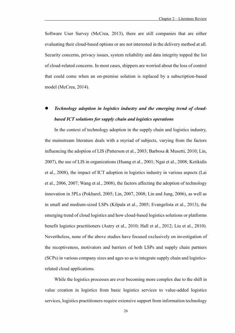
Figure 2.2 Dimensions being considered in order picking process (Goetschalckx and Ashayeri, 1989) 30
Figure 2.3 Time usage distribution during order picking 32
Figure 2.4 A typical CBR process 38
Figure 2.5 A generic AHP hierarchy structure 41
Figure 2.6 A n*n pairwise comparison matrix 41
Figure 2.7 A nine-point scale for pairwise comparison 41
Figure 2.8 Standard procedures of the GA operations 45
Figure 2.9 The merged membership functions in fuzzy logic technique 47
Figure 3.1 Order throughput difference with and without the application of WPS 71
Figure 3.2 Architecture of the EF-DSS 73
Figure 3.3 Consolidation and sorting of customer e-order in EF-DSS 76
Figure 3.4 E-order grouping and operating guidelines generation in EF-DSS 77
Figure 3.5 The generic format of a chromosome 79
Figure 3.6 An example of the shortest inter-bin travel distance calculation between two storage bins 80
Figure 3.7 E-order arrival prediction and cut-off time decision support generated by the EBRM 85
Figure 3.8 Architecture of ANFIS network 87
Figure 3.9 Fuzzy reasoning mechanism in ANFIS 87
Figure 4.1 The implementation procedures of the EF-DSS 102
Figure 4.2 An example of internal process investigation for logistics order handling (1) 104
Figure 4.3 An example of internal process investigation for logistics order handling (2) 104
List of Figures
xiii
Figure 4.4 An example of internal process investigation for logistics order handling (3) 105
Figure 4.5 An example of internal process investigation for logistics order handling (4) 105
Figure 4.6 An example of a system function and feature list 107
Figure 4.7 An example of the sorting algorithm for extracting the required inter-bin distances from the parent distance matrix 113
Figure 5.1 An overview of the research and case study setting 120
Figure 5.2 The underlying e-order information processing logic in ECM 125
Figure 5.3 Order picking operations in storage bin locations of e-fulfilment centers 125
Figure 5.4 Computer terminal for e-order consolidation and generating order grouping list 126
Figure 5.5 Order grouping decision support development using GA 127
Figure 5.6 Codes for distance matrix sorting 128
Figure 5.7 User interfaces of EF-DSS – Order consolidation and grouping 130
Figure 5.8 User interfaces of EF-DSS – Details of order grouping list and generating operating guidelines 131
Figure 5.9 Conceptual framework for ANFIS model construction for Case study 2 136
Figure 5.10 Lag test for identifying the number of lag length n 140
Figure 5.11 AR(1)MO(1) model structure 142
Figure 5.12 AR(1)MO(2) model structure 142
Figure 5.13 ANFIS model training and testing environment in MATLAB’s Neuro-fuzzy designer toolbox 144
Figure 5.14 User interface of the EF-DSS used in Case study 2 148
Figure 5.15 Conceptual framework for ANFIS model construction for Case study 3 153
Figure 5.16 Lag test for identifying the number of lag lengths n for the aggregated dataset 156
Figure 5.17 Lag test for identifying the number of lag lengths n for retailer 1 157
Figure 5.18 Lag test for identifying the number of lag lengths n for retailer 2 158
Figure 5.19 Lag test for identifying the number of lag lengths n for retailer 3 159
List of Figures
xiv
Figure 5.20 AR(1)MO(1)MA(2) model structure 168
Figure 5.21 AR(1)MO(1)MA(3) model structure 169
Figure 5.22 Model performance comparison framework 172
Figure 6.1 Graphical comparison of the results under different combinations of GA parameter setting 175
Figure 6.2 Improvement in terms of order processing time 177
Figure 6.3 Network frame of AR(1)MO(1) model using the best structure 181
Figure 6.4 Network frame of AR(1)MO(2) model using the best structure 181
Figure 6.5 Test results of AR(1)MO(1) model using the best structure 181
Figure 6.6 Test results of AR(1)MO(2) model using the best structure 182
Figure 6.7 Automatic ARIMA model selection result for case study 1 183
Figure 6.8 Forecast comparison graph showing the selected model (in red) and other ARIMA models (in grey) for case study 1 183
Figure 6.9 Comparison of actual and predicted e-order arrival using AR(1)MO(1), AR(1)MO(2) and ARIMA model for observation no. 1-42 184
Figure 6.10 Comparison of actual and predicted e-order arrival using AR(1)MO(1), AR(1)MO(2) and ARIMA model for observation no. 43-84 185
Figure 6.11 Test results of the best model (Model 1B) for retailer’s 1 dataset 190
Figure 6.12 Test results of the best model (Model 2B) for retailer’s 2 dataset 190
Figure 6.13 Test results of the best model (Model 3B) for retailer’s 3 dataset 190
Figure 6.14 Test results of the best model (Model 4B) for the dataset aggregating retailers 1, 2 and 3 191
Figure 6.15 A graphical comparison between actual and predicted e-order arrival figures for retailer 1 under Typology II 195
Figure 6.16 A graphical comparison between actual and predicted e-order arrival figures for retailer 2 under Typology II 196
Figure 6.17 A graphical comparison between actual and predicted e-order arrival figures for retailer 3 under Typology II 196
Figure 6.18 A graphical comparison between actual and predicted e-order arrival figures for aggregated dataset under Typology I 197
List of Figures
xv
Figure 6.19 Automatic ARIMA model selection result for the dataset aggregating all retailers’ data 200
Figure 6.20 Details of the ARIMA model selection result for the dataset aggregating all retailers’ data 200
Figure 6.21 Forecast comparison graph showing the selected model (in red) and other ARIMA models (in grey) (for the dataset aggregating all retailers’ data) 201
Figure 6.22 A graphical comparison between actual and predicted e-order arrival figures using ARIMA for the dataset aggregating all retailers’ data 201
Figure 6.23 Automatic ARIMA model selection result for retailer 1’s dataset 202
Figure 6.24 Details of the ARIMA model selection result for retailer 1’s dataset 202
Figure 6.25 Forecast comparison graph showing the selected model (in red) and other ARIMA models (in grey) (for retailer 1’s dataset) 203
Figure 6.26 A graphical comparison between actual and predicted e-order arrival figures using ARIMA for retailer 1 203
Figure 6.27 Automatic ARIMA model selection result for retailer 2’s dataset 204
Figure 6.28 Details of the ARIMA model selection result for retailer 2’s dataset 204
Figure 6.29 Forecast comparison graph showing the selected model (in red) and other ARIMA models (in grey) (for retailer 2’s dataset) 205
Figure 6.30 A graphical comparison between actual and predicted e-order arrival figures using ARIMA for retailer 2 205
Figure 6.31 Automatic ARIMA model selection result for retailer 3’s dataset 206
Figure 6.32 Details of the ARIMA model selection result for retailer 3’s dataset 206
Figure 6.33 Forecast comparison graph showing the selected model (in red) and other ARIMA models (in grey) (for retailer 3’s dataset) 207
Figure 6.34 A graphical comparison between actual and predicted e-order arrival figures using ARIMA for retailer 3 207

List of Tables
xvi
List of Tables Table 1.1 The impact of e-commerce business on various stakeholders 3
Table 1.2 A comparison between the nature of traditional logistics orders and e-commerce orders (Leung et al., 2016) 5
Table 2.1 A summary of the literature related to the conventional
warehousing and transportation activities 34
Table 3.1 Generic details of the information stored in database of the EF-DSS 75
Table 3.2 Notation table for quantitative model of EF-DSS 82
Table 3.3 Notation definitions for ANFIS network architecture 88
Table 3.4 Example of cycle time determination 93
Table 3.5 Justifications of the input variables of the ANFIS forecasting models 94
Table 3.6 An example of data set in 2-hour time interval 95
Table 3.7 A summary of the configurable model settings that need to be tested 96
Table 3.8 Notation definitions for the cut-off frequency decision support in EBRM 100
Table 4.1 Example of the data to be collected under “general order information” and “detailed order specifications” data category 109
Table 4.2 Example of the data to be collected under “inbound order SOP setup” and “outbound order SOP setup” data category 109
Table 4.3 Example of the data to be collected under “party master” and “party SKU master” data category 110
Table 4.4 Database construction for various e-logistics activities 111
Table 5.1 Types of data stored and collected in the database for the case company 124
Table 5.2 Example rules applied in the case company 129
Table 5.3 Test results of AR(1) and AR(7) model 140
Table 5.4 Real four-week e-order arrival (in kg) data in 2-hour time interval 141
Table 5.5 Training parameters of the ANFIS model 143
Table 5.6 Notation definitions for the cut-off frequency decision support in EBRM 147
List of Tables
xvii
Table 5.7 Test results of AR(1) and AR(8) model for aggregated dataset 156
Table 5.8 Test results of AR(1) and AR(8) model for retailer 1 158
Table 5.9 Test results of AR(1) and AR(4) model for retailer 2 159
Table 5.10 Test results of AR(1) and AR(8) model for retailer 3 160
Table 5.11 A summary of ANFIS models designed for Typologies I and II 161
Table 5.12 Eight-week e-order arrival (in kg) data in 3-hour time interval for Retailer 1 162
Table 5.13 Eight-week e-order arrival (in kg) data in 3-hour time interval for Retailer 2 164
Table 5.14 Eight-week e-order arrival (in kg) data in 3-hour time interval for Retailer 3 166
Table 5.15 Training parameters of the ANFIS model in Case study 3 168
Table 5.16 A summary of the ANFIS model training and testing results 170
Table 6.1 Optimal parameter settings for the Genetic Algorithm 175
Table 6.2 A before-and-after comparison in terms of order processing time 177
Table 6.3 The characteristics of the best structure of AR(1)MO(1) and AR(1)MO(2) model and their corresponding ANFIS information 180
Table 6.4 Error analysis for model comparison for case study 1 184
Table 6.5 Item accuracy comparison for case study 1 184
Table 6.6 A before-and-after comparison of e-order handling and resource management 186
Table 6.7 A summary of the ANFIS models developed in Case study 3 187
Table 6.8 Best model setting for each ANFIS model 189
Table 6.9 Another one-week e-order arrival dataset for Retailer 1 192
Table 6.10 Another one-week e-order arrival dataset for Retailer 2 192
Table 6.11 Another one-week e-order arrival dataset for Retailer 3 192
Table 6.12 The one-week e-order arrival dataset that aggregates e-order arrival for Retailer 1, 2 and 3 193
Table 6.13 Error analysis for model comparison for Model 1B to 4B 195
Table 6.14 Item accuracy comparison for Model 1B to 4B 195
Table 6.15 Error analysis for model comparison for typology I and II 198
Table 6.16 Item accuracy comparison for typology I and II 198

List of Tables
xviii
Table 6.17 Error analysis for ARIMA model comparison 209
Table 6.18 Item accuracy comparison for ARIMA models 209
Table 6.19 Error analysis for ANFIS and ARIMA model comparison in typology II 210
Table 6.20 Item accuracy comparison for ANFIS and ARIMA model comparison in typology II 210
Table 6.21 Error analysis for ANFIS and ARIMA model comparison in typology I 211
Table 6.22 Item accuracy comparison for ANFIS and ARIMA model comparison in typology I 212
Table 6.23 A summary of the practical recommendation of the deployment of ANFIS forecasting models for the e-order arrival prediction 215
Table 6.24 Various scenarios of ineffective warehouse postponement strategy 218
Table 7.1 A list of potential application areas of the proposed AR-MO-MA-based ANFIS forecasting approach 226

List of Abbreviations
xix
List of Abbreviations
3PL Third-party Logistics
AHP Analytic Hierarchy Process
AI Artificial Intelligence
ANN Artificial Neural Network
AR Autoregressive
ARIMA Autoregressive Integrated Moving Average
ARMA Autoregressive Moving Average
AR-MO-MA-ANFIS Autoregressive-momentum-moving average-based
Adaptive Network-Based Fuzzy Inference System
B2B Business-to-business
B2C Business-to-customer
CBR Case-based Reasoning
DM Data Mining
E-order E-commerce Order
EBRM E-order Batch Releasing Module
EDI Electronics Data Interface
EF-DSS E-commerce Fulfillment Decision Support System
ECM E-order Consolidation Module
EGM E-order Grouping Module
ERP Enterprise Resource Planning
FIS Fuzzy Inference System
GA Genetic Algorithm
GDP Gross Domestic Product
IT Information Technology
ICT Information Communication Technology
IOT Internet-of-things
LIS Logistics Information System
LSP Logistics Service Provider
MA Moving Average
MO Momentum
MCDM Multiple Criteria Decision-Making

List of Abbreviations
xx
NNR Nearest Neighbor Retrieval
O2O Online-To-Offline
OMS Order Management System
RFID Radio Frequency Identification
SaaS Software-As-A-Service
SARIMA Seasonal Autoregressive Integrated Moving Average
SKU Stock-Keeping Units
TMS Transportation Management Systems
WPM Weighted Product Model
WPS Warehouse Postponement Strategy
WMS Warehousing Management System
WSM Weighted Sum Model

Chapter 1 – Introduction
1
Chapter 1 – Introduction
1.1 Research Background
The wider applications of the Internet for online shopping in recent decades have
brought enormous growth potential for international business-to-business (B2B) and
business-to-customers (B2C) trading. Shopping via multiple channels has become a
rapidly growing phenomenon. On one hand, companies continually add new sales
channels. On the other hand, end consumers and business entities can make purchases
using any of their mobile devices at any time. Since the beginning of 21st century, the
idea of “online shopping” that was expanded globally has already brought a series of
benefits for the stakeholders, especially the end consumers, wholesalers and retailers.
However, some drawbacks are perceived by the stakeholders under the e-commerce
business environment, as suggested in Table 1.1. B2B and B2C e-commerce have had
a profound impact on stakeholders along a supply chain, such as manufacturers,
retailers and logistics service providers (LSPs) (Gunasekaran & Ngai, 2004; Johnson
& Whang, 2002). In the perspective of manufacturers, the trend of online shopping
opens up the opportunity for them to directly sell their finished goods to end
consumers via their e-commerce shopping sites. This, in turn, threatens the position of
wholesalers and retailers as manufacturers are no longer required with wholesalers and
retailers as the middleman (Abhishek et al., 2015). As for LSPs, the e-commerce
logistics business is a huge market to capture. However, successful transformation of
the traditional logistics business to e-commerce for gaining the market share can be
achieved only if LSPs strengthen their internal order processing capability to handle
e-commerce orders (e-orders).
The motivations for LSPs to improve their core competence in order handling
under the e-commerce logistics business is twofold. First, the market for the traditional
Chapter 1 – Introduction
2
logistics business is to a certain extent quite mature. The e-commerce logistics
business is a new market segment in recent decades that has a large growth potential,
with the fact that consumers have started perceiving online sales platforms as one of
the major channels for making a purchase (Carlson et al., 2015; Falk & Hagsten, 2015).
In light of the continuous B2B and B2C e-commerce growth, the underlying logistics
e-order processing operations, such as e-order fulfillment in distribution centres and
last-mile delivery of parcels, are in great demand. Second, the rise of such online-to-
offline (O2O) retailing and e-commerce business has revamped the entire order
fulfilment process along supply chains (Lekovic & Milicevic, 2013). At the
operational level, LSPs are struggling with the problem of e-commerce order handling
inefficiencies in warehouses or distribution centers (Lang & Bressolles, 2013), which
is largely attributed to the difference between e-commerce orders and traditional
orders. As shown in Table 1.2, i.e. a summary of a comparison between the
characteristics of traditional logistics orders and e-commerce orders, there are vast
differences between these orders in terms of the nature of the order, size per order,
stock-keeping units involved in each order, number of orders received within a
timeframe, arrival frequency, time availability for processing, and the delivery
schedule. Traditionally, logistics orders processed in warehouses are mainly initiated
from retailers who require stock replenishment for specified physical stores. Each of
these traditional orders involves only a few types of stock-keeping units (SKUs), but
in large quantity. In contrast, e-commerce orders are placed by end consumers
worldwide via e-commerce selling platforms, which exhibit very different order
characteristics as each e-order involve a large number of SKUs, but with each SKU
demanding only a very small quantity. Also, these e-orders are significantly more
wide-spread in terms of delivery location. Adding the requirement of same-day or
next-day delivery for e- orders, the e-commerce logistics business model is now more

Chapter 1 – Introduction
3
complex and dynamic than the traditional one. Previous studies have already
addressed the difficulty for LSPs to manage warehouse operations and last-mile order
fulfilment without strategic and operational transformation (Hultkrantz & Lumsden,
2001; Cho et al., 2008; Lang & Bressolles, 2013). Therefore, taking the above-
mentioned motivations into account, there is a crucial need for LSPs to strength their
core competencies for e-order handling in order to capture the e-commerce logistics
market pie. On the other hand, however, they can no longer follow the conventional
order fulfilment process in handling e-commerce orders due to the fundamental
differences between conventional and e-commerce logistics orders.
Table 1.1. The impact of e-commerce business on various stakeholders
End consumer
Positive impacts Negative impacts
Convenience, better prices, and
wider range of products and services
– Ease of performing benchmarking
in the selection of retailers or
products due to the higher degree of
product information and pricing
Fake or low-quality products – The
inability of physical inspection of
products by consumers
Privacy concerns – Purchasing
habits, delivery address, personal
details are all stored at the database
of e-commerce sites
Retailers
Positive impacts Negative impacts
Maximizing revenue while reducing
the operating expenses – smaller
operating space requirements, less
staff
Enlarged consumer base - the
opportunity to be visible and visited
by more customers
Intense competition – Ease of
entering the market indicates the
existence of a large number of direct
competitors
Decline of being a middleman
between manufacturers and end
consumers – The emerging e-
commerce business models close the

Chapter 1 – Introduction
4
Low barriers to entry – Ease of
entering the e-commerce market at
low operating costs
gap between manufacturers and end
consumers
Manufacturers
Positive impacts Negative impacts
Forward integration – By extending
its role from manufacturer to retailer
in the supply chain through e-
commerce
Better cost control and inventory
management – Reduce the bullwhip
effect with the shortened supply
chains
Lack of knowledge – Diversified
focus on core business, hard to take
the role as distributor
Logistics service providers
Positive impacts Negative impacts
E-commerce logistics business as a
new market segment to target –
Opportunity to capture new e-
commerce logistics market
A greater role to play in e-commerce
marketplace – Last-mile delivery and
e-commerce order handling are the
keys to customer satisfaction in
online shopping
Strict delivery requirements phasing
out traditional LSPs with low
operating efficiency – Requires LSPs
to keep up with the pace of e-
commerce development by enhancing
internal order handling efficiency
Difficulty in business transformation
from traditional LSPs to e-commerce
based LSPs – A gap exists between
enormous e-commerce order volume
and logistics order handling ability
Chapter 1 – Introduction
5
Table 1.2. A comparison between the nature of traditional logistics orders and e-
commerce orders (Leung et al., 2016)
Order characteristics Traditional
logistics orders
E-orders placed by end
customers electronically
Nature of order Mostly stock replenishment Fragmented, discrete
Size per order In bulk In small lot-size
SKUs involved in each
order Very few or even identical Many
Number of orders
pending for processing Less, relatively easy to predict
More and unlimited, relatively
difficult to predict
Arrival frequency of
order Regular Irregular
Time availability for
fulfilment Less tight Very tight
Delivery schedule Relatively more time buffer Next-day or even
same-day delivery
1.2 Problem Statement
The need for an introduction of Warehouse Postponement Strategy
Given the huge market potential of the e-commerce logistics business, the
existing operational inefficiencies in e-order handling in warehouses and distribution
centres lead to major bottleneck for LSPs to capture the e-commerce business
opportunities (Mangiaracina et al., 2015). Therefore, in this research, the need for
LSPs to re-engineer their order processing flow for streamlining e-commerce order
handling is addressed. Without the re-engineering of the order fulfillment process for
today’s e-commerce business, there are two significant problems in the existing
operations, as shown in Fig. 1.1, they are:
Chapter 1 – Introduction
6
(i) Inefficiency of e-commerce order handling due to frequent and discrete arrival
of orders
In today’s e-commerce retail industry, customers are guaranteed in advance to be
able to receive the items before a specified date or within the timeslot they selected.
Facing the tight delivery requirements, LSPs are required to handle e-orders extremely
efficiently. ‘Efficient e-order handling’, ‘speed’ and ‘accuracy’ are the critical
performance indicators of LSPs (Krauth et al., 2005; Gunasekaran et al., 2004). Not
only do they have to be capable of processing a large number of e-orders accurately
within the specified time constraints to meet the customers’ or retailer’s delivery
requirements, but they are also required to be agile enough in handling the fluctuating
arrival of incoming e-orders. In turn, effective resource management can be achieved
through better utilization or allocation of available resources, such as manpower and
material handling equipment, in various order arrival periods throughout the working
hours. For instance, as depicted in Fig. 1.1, during the peak period of e-order arrivals,
customer service representatives process the received e-orders accordingly and send
the order details to the distribution centres for actual order fulfilment, which involves
warehouse workers picking the ordered items from the corresponding storage
locations and packing the items according to the customer order. The problems of such
a conventional order handling process lie in the difficulty for warehouse workers to
handle a large number of discrete e-orders individually. It is almost impossible for the
workers handle fragmented e-orders one-by-one.
(ii) Lack of mechanism for data pre-processing of e-commerce orders
In the case of Hong Kong, being a global transhipment hub, LSPs are shifting
their business to an e-commerce orientation owing to the fast growing trend of e-
business in Asia. However, most of the logistics practitioners lack an effective
Chapter 1 – Introduction
7
mechanism for e-commerce order pre-processing, as their operations are still manual
and without IT support. E-commerce orders are handled in the same conventional way
as for traditional logistics orders.
(iii) Lack of cost effective decision support tools to facilitate e-commerce logistics
operating procedures
The frequent and discrete arrival of e-commerce orders, one of the biggest
differences as compared to the traditional logistics orders, has resulted in e-commerce
order handling in e-fulfilment centres being inefficient. There is a lack of lightweight,
cost effective IT solutions that are specifically designed to handle e-commerce orders
which are received from the Internet. The core reason for this is the lack of domain
know-how by IT solution developers in the e-commerce supply chain field, thereby
being unable to identify the B2C e-commerce order handling difficulties currently
faced by the logistics practitioners.
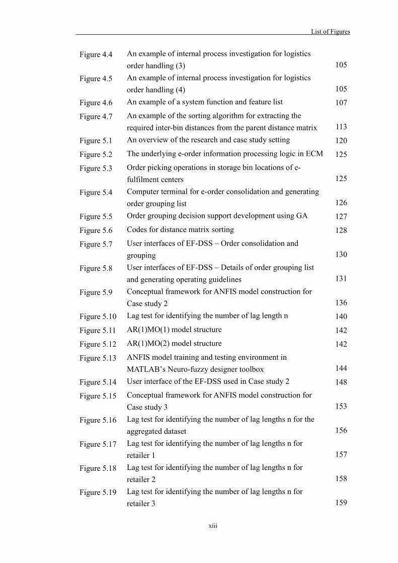
Fig. 1.1. Order fulfillment bottlenecks under today’s e-commerce operating
environment

Chapter 1 – Introduction
8
Consequently, the absence of a mind-set from the managerial perspective and an
effective mechanism in the operational perspective for order pre-processing has
created barriers for logistics practitioners to engage in the e-commerce logistics
business. Further, not only does the internal incapability of efficient e-order handling
become the major obstacle in business expansion, but it is also a bottleneck in the
entire e-commerce supply chain which affects the efficiency of e-fulfilment of the
downstream supply chain partners. This explains why the last-mile delivery in e-
commerce, the final leg of the complete journey of a parcel before it reaches the
customer, is regarded as one of the biggest challenges in today’s e-commerce business.
In view of the necessity of logistics process re-engineering under the emerging
e-commerce logistics business environment, this research identifies the need to extend
the wider concept of “postponement strategy” to the warehouse operational level, by
not only conventionally delaying the configuration and assembling of a product in the
manufacturing perspective, but also at the warehouse operational level “delaying the
execution of a logistics process until the last possible moment”. The “delay of a
logistics process execution until the last possible moment” is defined as “warehouse
Postponement Strategy” (WPS) in this study. In theory of WPS, the throughput rate in
a distribution centre from a fluctuating pattern is rearranged to one that follows a
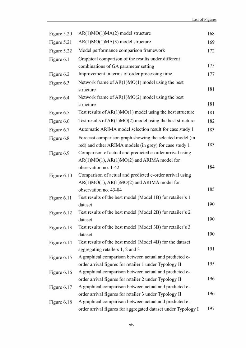
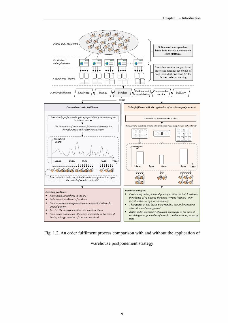
regular wave pattern, as presented in Fig. 1.2.
Chapter 1 – Introduction
9
Fig. 1.2. An order fulfilment process comparison with and without the application of
warehouse postponement strategy

Chapter 1 – Introduction
10
The current research and practical gap in deploying WPS
The concept of WPS can be achieved by grouping e-orders in a consolidation
pool, and then subsequently releasing the grouped e-orders for processing at the same
time. By means of bulk processing, different e-orders that consist of the same item(s)
can be picked from the designated storage location(s) of the distribution centre at the
same time. Such practice best suits the nature of e-order handling, as these frequently
arrived e-orders are fragmented, discrete and smaller lot-sized. Therefore, deploying
WPS for bulk e-order handling not only rearranges the throughput rate in a distribution
centre, but also benefits logistics practitioners in terms of order processing efficiency,
resource management and workforce level adjustment. A noticeable advantage of the
deploying WPS is the reduction of the possibility for a worker to re-visit the same
storage location throughout the working hour. In the absence of WPS deployment,
order pickers are required to process each e-order individually. Hence, the order
pickers are very often required to visit the same storage locations for those popular
items which are frequently ordered by individual consumers. Traveling to repetitive
storage locations is a type of operating inefficiency due to improper order planning.
Therefore, a logistics practitioner can perform better order planning through the
introduction of WPS. However, for effective deployment of WPS, the following two
conditions are critical:
(1) How e-orders are grouped for later batch processing; and
(2) When should a decision-maker stop consolidating e-orders and release the
consolidated e-orders for actual batch processing.
While the above WPS deploying conditions determine the success of logistics re-
engineering for the e-commerce operating environment, the decision support proposed
in the mainstream literature in facilitating e-commerce logistics operations has been

Chapter 1 – Introduction
11
lacking. A majority of the expert systems proposed in previous studies in the domain
of warehousing and transportation process improvement, such as Oliveira et al. (2015),
Patriarca et al. (2016), Gu et al. (2016), Yang et al. (2015), Accorsi et al. (2014), Lam
et al. (2011), Poon et. al. (2011), Yao et al. (2010), Zacharia & Nearchou (2010),
Taniguchi & Shimamoto (2004), Chan et al. (2009) and Chen et al. (2008), focus only
on tackling a specific operational issue in warehouses or distribution centers in
handling general logistics orders. However, without consideration of the differences
in the nature and handling requirements between e-commerce orders and conventional
logistics orders, previous expert systems might not be applicable to the scenario of
today’s e-commerce order handling process. Furthermore, Nguyen et al. (2018)
suggested that very little research in the mainstream literature has been conducted to
manage e-commerce order fulfilment activities better. Mangiaracina et al. (2015) also
suggested that, the environmental implications of the related logistics activities have
not yet been studied in detail, despite logistics practitioners playing an emerging role
of multichannel strategies in e-commerce.
1.3 Research Objectives
In view of the crucial necessity to re-engineer the logistics operational flow for
improved e-order handling in warehouses and distribution centers, this research
proposes an operational strategy, namely “Warehouse Postponement Strategy”. For
successful implementation of WPS in a real production environment of LSPs, it is
suggested that two conditions, i.e. (1) How e-orders are grouped for later batch
processing (How to group), and (2) When should a decision-maker stop consolidating
e-orders and releasing the grouped e-orders must be deeply considered, as shown in
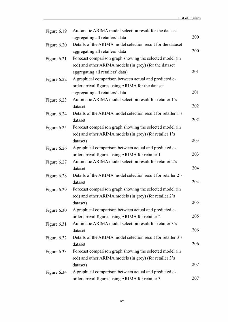
Fig. 1.3. Therefore, this research develops a decision support system for assisting the

Chapter 1 – Introduction
12
LSPs in making prompt decisions regarding (1) How to group, and (2) When to release.
The specific objectives of this research are:
(i) To re-engineer the internal order processing flow for LSPs to improve their
core competencies in e-order handling;
(ii) To provide decision support solutions to properly deal with the issue of “How
to group” and “When to release” for successful deployment of the proposed
Warehouse Postponement Strategy; and
(iii) To present a generic system architecture so as to enable a LSP to implement
WPS based on their specific size of e-commerce logistics business.
Fig. 1.3. The focus of this research
1.4 Significance of the Research
Traditional approaches proposed in the literature rarely took the e-commerce
logistics environment into account, rendering the previous proposed expert systems
inapplicable to the current e-commerce logistics business. Moreover, previous studies

Chapter 1 – Introduction
13
attempted to manage productivity in warehouses and distribution centres by means of
resource management and effective order planning, such as the development of IOT-
based or RFID-based solutions for logistics order and resource track and trace in
warehouses, and heuristics solutions using artificial intelligence, data mining
approaches, or mathematical modelling approach for streamlining the conventional
order processing flow. Resource management and order planning in conventional
logistics warehouses have been widely and adequately researched. Under the ever
complex and dynamic order handling environment in today’s e-fulfilment centre,
productivity management in logistics can be performed not only by means of resource
management and order planning, but also through logistics order arrival prediction.
Logistics order arrival prediction is a new subject that has attracted sparse
attention by both researchers and industry practitioners as conventional logistics
orders arrive at the warehouses in a regular time interval. However, under the dynamic
e-commerce logistics business, forecasting the irregular arrival pattern of fragmented
and discrete e-orders becomes an essential subject for LSPs to identify “When to
release the grouped e-orders”, one of the conditions of deploying WPS. Thus, this
research fills the existing gap in the literature and opens up a new research area in the
field of e-commerce-based order management under today’s customer-driven supply
chain, by addressing the need to forecast e-order arrival for formulating a proper
Warehouse Postponement Strategy for improved order planning and execution. This
research is a new study that introduces a novel autoregressive-momentum-moving
average-based Adaptive Network-Based Fuzzy Inference System (AR-MO-MA-
ANFIS) approach, integrating the nature of autoregressive feature of time series data
into an ANFIS model for improving the operating efficiency in the context of supply
chain management, by means of forecasting the arrival of e-commerce orders.

Chapter 1 – Introduction
14
In addition to the integrated AR-MO-MA-ANFIS approach for the prediction of
e-order arrival figures, the framework of the proposed system in this research provides
a step-by-step implementation flow of WPS, enabling logistics practitioners to
efficiently manage a large number of discrete, small lot-sized e-orders in distribution
centers, which is a phenomenon that commonly exists in today’s order fulfilment
operations. In turn, the re-engineering of logistics operational flow in handling e-
commerce orders can be achieved. This would be beneficial for various stakeholders
along the supply chains. LSPs would become more capable in capturing the logistics
of the e-commerce business due to higher efficiency in e-order handling. Retailers can
build brand images and loyalty by satisfying the consumers’ needs and expectations,
especially considering the timeliness of the last-mile e-order delivery, one of the most
critical e-fulfilment processes. End consumers can receive their purchased items
without a long waiting time.
1.5 Thesis Outline
The thesis is divided into seven chapters, as described below.
(i) Chapter 1 introduces the background of the research. The problem definitions
under the e-commerce operating environment of LSPs, the motivations and
significance of this research are also discussed.
(ii) Chapter 2 provides an academic review of the related research, including a
comprehensive review of the current e-commerce logistics operating
environment, and the existing bottlenecks of e-order handling activities in
warehouse and distribution centres. The analysis of decision support systems and
existing approaches, such as the application and integration of artificial
intelligence and data mining techniques, and time-series data analytical tools,
adopted in warehouse activities are discussed and reviewed.

Chapter 1 – Introduction
15
(iii) Chapter 3 is divided into two main sections. The first section introduces the
architecture of the proposed system, namely the E-commerce Fulfillment
Decision Support System (EF-DSS). The second section describes the
infrastructure of EF-DSS, which consists of an E-order consolidation module
(ECM), an E-order grouping module (EGM), and an E-order batch releasing
module (EBRM). The development of these system modules realizes the
proposed concept of “Warehouse Postponement Strategy” by “delaying the
logistics process execution until the last possible moment”, so as to enable
logistics practitioners to improve the internal core competencies in e-order
handling activities.
(iv) Chapter 4 provides a generic implementation guide of EF-DSS from the design
stage, through the structural formulation of each module, to the implementation
and evaluation stage. This framework allows industry practitioners to deploy the
WPS according to their size of e-commerce logistics business.
(v) Chapter 5 presents three case studies in which EF-DSS is developed and
implemented in three different Hong Kong-based third-party logistics service
providers, in order to demonstrate the feasibility of the proposed methodology in
managing e-commerce orders. An EF-DSS software prototype is developed and
the related operating mechanism for supporting the decision-making process is
also discussed.
(vi) Chapter 6 discusses the results and major findings of the research. The system
performance and parameter settings for obtaining the best system parameters are
presented, followed by a discussion of the overall operating performance of the
case companies after the pilot implementations of EF-DSS.
(vii) Chapter 7 concludes the work undertaken in the research. Contribution made by
the research and key areas for future research are highlighted.

Chapter 2 – Literature Review
16
Chapter 2 – Literature Review
2.1 Introduction
The focus of this research is on the design of a E-fulfilment decision support
system for re-engineering the operational flow of e-commerce operations in
distribution centres. To achieve this, a comprehensive review on the background of
supply chain management under e-commerce business environment and the data
mining and artificial intelligence techniques for heuristics problem-solving is required.
The aim of this chapter is to examine the previous literature related to the current
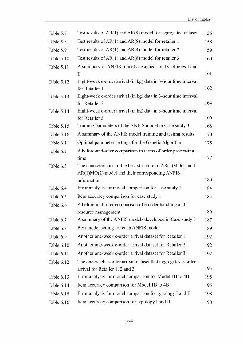
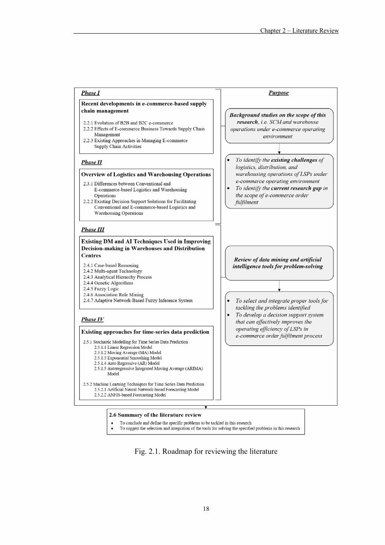
research areas. Figure 2.1 depicts the roadmap for reviewing the related literature. In
this chapter, there are four phases of the review of the literature. The purpose of the
first two phases is to comprehensively review the background and scope of the
research areas of this research, i.e. supply chain management and warehousing
operations under e-commerce operating environment. Through the background studies,
the existing challenges of logistics, distribution, and warehousing operations under e-
commerce operating environment are discussed and identified, so as to identify the
existing research gaps in the literature. For instance, Phase I, i.e. Recent Developments
in E-commerce-based Supply Chain Management, covers three sections: Section 2.2.1
- Evolution of B2B and B2C E-commerce, Section 2.2.2 - Effects of E-commerce
Business Towards Supply Chain Management, and Section 2.2.3 - Existing
Approaches in Managing E-commerce Business Activities. For Phase II, i.e. Overview
of Logistics and Warehousing Operations, it covers two sections: Section 2.3.1 - The
Differences between Conventional and E-commerce-based Logistics and
Warehousing Operations, and Section 2.3.2 - Existing Decision Support Solutions for
Facilitating Conventional and E-commerce-based Logistics and Warehousing
Operations.

Chapter 2 – Literature Review
17
A comprehensive review of the existing tools for improving the decision-making
process in warehouses and distribution centers and for time-series data prediction is
performed in Phase III and IV. Through the review of the literature, appropriate tools
can be selected and suggested in this chapter for achieving the objectives of this
research, i.e. developing a decision support system to improve the operating efficiency
of LSPs in handling e-commerce orders in distribution centers. In Phase III - Existing
DM and AI techniques Used in Improving Decision-Making in Warehouses and
Distribution Centers, in total there are seven techniques reviewed, including case-
based reasoning, multi-agent technology, analytical hierarchy process, genetic
algorithms, fuzzy logic, association rule mining, and adaptive network-based fuzzy
inference system (Section 2.4.1 to Section 2.4.7). Apart from reviewing these data
mining and artificial intelligence techniques, approaches for forecasting time-series
data are also reviewed, so as to select proper tools for forecasting the e-order arrival
pattern to assist LSPs’ in determining the “when to release grouped e-orders” decision,
one of the objectives of this research. Therefore, in Phase IV - Existing approaches for
time series data prediction, stochastic modelling approaches including linear
regression, moving average (MA), exponential smoothing, auto regressive (AR), and
autoregressive integrated moving average (ARIMA) model, are reviewed in Section
2.5.1. Machine learning techniques for time series data prediction including ANN-
based and ANFIS-based forecasting models, are reviewed in Section 2.5.2. Lastly,
conclusions are drawn in Section 2.6 – Summary, to provide insight on the research
direction and discuss the traits of the E-fulfilment decision support system proposed
in this research study.
Chapter 2 – Literature Review
18
Fig. 2.1. Roadmap for reviewing the literature
Chapter 2 – Literature Review
19
2.2 Recent Developments in E-commerce-based Supply Chain
Management
The development of supply chain management has been drastically affected by
the emerging shift of consumer buying behavior, owing to an increasing trend of online
shopping experience in which retailers around the globe are struggling to deliver to
consumers worldwide. In this section, a review of the evolution of B2B and B2C e-
commerce, the effects of e-commerce business activities towards modern supply chain
management, and the existing approaches in managing e-commerce supply chain
activities, are presented.
2.2.1 Evolution of B2B and B2C E-commerce
From the perspective of B2B e-commerce, business transactions are
conventionally made through face-to-face meetings, phone calls and emails. The
advancement of information technology (IT) enables enterprises to place orders via
the Internet. Such contactless transactions made via the Internet have become a major
sales channel for suppliers. In 2017, the gross merchandise volume of business-to-
business e-commerce transactions amounted to 7.66 trillion U.S. dollars, up from 5.83
trillion U.S. dollars in 2013 (Statista, 2017). While the rise of B2B online retail stores
creates more potential business opportunities due to the increase of brand exposure of
suppliers to the potential customers worldwide, suppliers are forced to improve their
efficiency in the internal business process, such as the Request for Quotation process
(García-Crespo et al., 2009; Hvam et al., 2006), that supports the front line
management of e-commece.
Over the past decade, e-commerce has bought a whole new era to the retail
business. The drastic growth of e-commerce is attributed to the evolution of hardware
and the internet, with both having a direct correlation with today’s e-commerce. The

Chapter 2 – Literature Review
20
emerging e-commerce not only revolutionised the retail industry, the way sellers sell
their products and the way we buy and source products, but also the way we
communicate with each other and the way companies perform marketing activities,
especially making advertising. Social media, a computer-based technology that
facilitates the sharing of ideas and information, is one of the hottest trends in the past
decade. The use of social media has been extended from individual’s use of
communication and interaction with others to the use by business entities. With an
enormous base of active users, social media platforms create a large base for marketers
to utilize these platforms for achieving their marketing purposes, such as increasing
brand exposure, building customer relationship, and implementing target marketing
strategies. Social media has evolved to be a new hybrid element of the promotion mix
(Mangold & Faulds, 2009).
The current directions of the e-commerce retail and logistics industry
development are summarized below.
(i) New product categories for e-commerce business – The most popular
product category for selling through online sales channels is computer and consumer
electronics. Industry reports and statistics indicate that food and beverage is an
upcoming trendy product category for e-commerce, which will drive e-commerce
growth in the near future (Food Dive, 2016). The delivery of food and beverage
products requires different skill sets and technologies as compared to the handling of
traditional fast moving consumer goods (FMCGs). The food produce must be
monitored closely along the entire cold supply chain. Higher requirements in terms of
delivery timeliness, hygiene conditions in delivery, and temperature control are also
expected.

Chapter 2 – Literature Review
21
(ii) The mobility trend for mobile and social commerce – Marketing research
conducted by Global Web-Index (GWI) (2017) underscored how mobile applications
(Apps) and Internet users in the Asia-Pacific region are taking a lead in social
commerce. In contrast to only 67% of the Facebook users being interested in online
shopping, 81% of WeChat users and 79% of Sina Weibo users have been participating
in online shopping. In Asia, affluent audiences embrace new technologies at a fast
pace. Technologically, mobile apps for mobile and social commerce are also being
rapidly developed in Asian countries as one of the motivators of Internet users
participating in online shopping via apps. With the “Buy now” option available on
more social media platforms, such a mobile and social commerce trend is promising.
(iii) The convergence trend – Global internet companies are at a stage of
enterprise cooperation, mergers and reorganizations. Examples in mainland China
include Dangdang being merged with Taobao Mall, and Alibaba integrated with
Meituan. Due to the similar marketing positioning of the e-commerce sites, mergers
and reorganizations reduce the number of competitors in the market, reduce any
potential duplication of resources, and jointly enhance the overall competitiveness and
bargaining power.
2.2.2 Effects of E-commerce Business Towards Supply Chain Management
In the past decades, the logistics industry has been facing numerous operational
challenges. First, the mode of production has been transformed from the traditional
mass production into the mass customization production mode to facilitate increasing
global market competition (Chow et al., 2006). In order to adapt to such change to
achieve competitive advantage, warehouses need to be redesigned and automated to
achieve higher productivity and throughput, thereby reducing the order processing

Chapter 2 – Literature Review
22
cost (Harmon, 1993). The adoption of new philosophies such as Just-In-Time (JIT)
and lean production has brought dramatic changes in the functions and operations of
warehouses to minimize stock with tighter inventory control policies and shorten the
response time (Gu et al., 2007). Second, the emerging trend of e-commerce business
also poses serious challenges in the field of logistics. As e‐commerce shipments
require an entirely new distribution infrastructure to handle online business (Cho et al.,
2008), warehouses must be able to efficiently pick and pack single items and small
volume orders, and deliver them in small parcel shipments at a higher frequency to
consumers. In this sense, traditional order fulfillment which encompasses receiving,
put-away, picking, transport through the warehouse or distribution center, might not
be able to fully meet the requirements of e-commerce.
The supply chain network is becoming increasingly complex as e-commerce and
omni-channel retailing has opened up the retail industry to new customer demands and
market segments. Manufacturers who conventionally sell their products to wholesalers,
i.e. the middleman between manufacturers and retailers, can sell their finished
products directly to end consumers via launching online retail stores. Such vertical
integration of manufacturers reshapes not only the traditional product flow within a
supply chain, but also logistics practices in handling these online orders. The
development of the e-commerce retail segment has been brought to the next level with
the rise of mobile payment (Narang & Arora, 2018). The convenience brought by
seamless mobile payment allows consumers to shop and pay at anytime and anywhere.
As worldwide consumers are able to purchase items online, the success of B2C and
B2B e-commerce trading requires the full cooperation between the e-retailers and the
logistics service providers. LSPs are required to handle underlying logistics,
warehousing and distribution process for the purchased items to cross borders and
deliver to the destinations.

Chapter 2 – Literature Review
23
2.2.3 Existing Approaches in Managing E-commerce Supply Chain Activities
In the real logistics business environment, supply chain and logistics information
management systems, also referred to as logistics information systems (LISs), are
engineered and designed for logistics service providers to manage the available
information in the supply chain for effective resource allocation and management of
the physical flow of goods. They accommodate not only functions such as purchasing,
warehousing and transportation, but also extensive connections with external partners
(Sahin & Robinson, 2002), and engage customers to compete in the volatile and
interconnected economy (Luo, 2013). Replacing phone, fax and e-mail to an
increasingly degree, electronics data interface (EDI) automatically exchanges data
between transactional parties. EDI is considered an indispensable capability for
logistics functions to be coordinated with the operations of their partners and
customers.
Typical LISs are warehousing management systems (WMS), transportation
management systems (TMS), enterprise resource planning (ERP), etc. They substitute
manual work or eliminate inefficient human effort and improve managerial decision
making processes (Helo & Szekely, 2005). They streamline business processes (Faber,
2002), significantly reduce operation errors and enable the review of past performance,
monitoring of current performance and prediction of future demand (Liu et al., 2005).
With the integration of artificial intelligence technologies, LISs have the potential to
help managers make complicated decisions by providing processed data of past cases.
According to the annual analysis of the global WMS market conducted by the ARC
Advisory Group (2014), retailers and manufacturers are “exerting demand on the
WMS market whether from direct purchase of WMS solutions or through the
extension of contracts with third-party logistics (3PL) providers so as to support their
fulfillment operations”. The ARC Advisory Group expects continuous expansion of
Chapter 2 – Literature Review
24
omni-channel commerce and fulfillment in the coming years. WMS solutions are
identified as a core enabler of omni-channel fulfillment.
However, the existing LIS solutions in the market, such as WMS, have little or
no functionality that is integrated with AI technologies for enabling users in the
decision-making of resources allocation and optimization (Accorsi et al., 2014; Poon
et al., 2009). WMS are incapable of real-time information capturing or the actual
working status visualization (Huang, 2007). Hence, data input must be done manually
by operators, either via direct input into the system or by using handheld devices to
capture data using barcodes, and then transfer the data via wireless network
connections. As a result, the absence of decision-support functionality and a real-time
information capturing ability reduces the overall efficiency of the order fulfillment
process at the distribution centre or warehouse.
The essence of information and communication technology for the supply
chains
In the global marketplace, the internet facilitates enormous business opportunities
and is a prerequisite to develop technology-driven competitive advantage (Liu &
Orban, 2008). With the maturity of Internet technology and the growing presence of
WiFi and 4G-LTE wireless Internet access, the evolution towards ubiquitous
information and communication networks is apparent. This leads to a paradigm shift
from the use of traditional on-premise software systems to internet-based cloud
computing model (Gubbi et al., 2013; Sasikala, 2011). On-demand software, referred
to as software-as-a-service (SaaS), a completely innovative software application
model, started to become popular at the beginning of the 21st century. End-users can
choose and subscribe the software according to their actual needs so as to have the
permission to use the software in a specified period of time (Buyya et al., 2013).

Chapter 2 – Literature Review
25
Gartner (2013) defined SaaS as “Software delivered remotely and managed by a third
party as a one-to-many service through subscription or pay for use.” Being widely
recognized as a monumental enabler for business collaboration (Chen et al., 2007), the
use of information technology and systems across diverse fields for routine operations
and its reliance is growing (Shaikh & Karjaluoto, 2015). According to the ‘Information
Technology (IT) Spending Forecast’ published by Gartner (2014), worldwide dollar-
valued IT spending will grow 3.2% in 2014, reaching USD 3.8 trillion. ‘Trends and
Directions of SaaS in Asia/Pacific’, another report published by Gartner (2013),
addressed that SaaS for supply chain management including warehouse management,
transportation management, sourcing and e-procurement, is within the top 10 SaaS
applications in Asia pacific region in terms of the current usage.
As flexibility is known to be a decisive element of effective supply chain
management (Duclos et al., 2003; Fredericks, 2005; Swafford et al., 2006), the cloud’s
scalability, ease of deployment and lowered cost of ownership enable cloud-based
software solutions for supply chain and logistics industry to be more useful in the
collaborative supply chain context (Boyer & Hult, 2005). The “pay per use” feature of
SaaS which allows users to pay according to the actual usage, is an advantage for
logistics operators due to cost reduction perspective they tend to focus on.
Nevertheless, the uncertainties of IT implementation (Autry et al., 2010; Prater, 2005)
and the slow pace of new technology adoption and innovation (Crum et al., 1996;
Evangelista & Sweeney, 2006; European Commission, 2012; McKinnon, 2009) have
been the obstacles faced by logistics operators. McDivitt, vice president and supply
chain technologies leader for Capgemini North America, suggested that the cloud
makes the most sense for shippers that intend to collaborate with external entities.
However, the apprehension still lies in the thought of sharing data in the public cloud
(McCrea, 2014). According to findings of Logistics Management’s 11th Annual
Chapter 2 – Literature Review
26
Software User Survey (McCrea, 2013), there are still companies that are either
evaluating their cloud-based options or are not interested in the delivery method at all.
Security concerns, privacy issues, system reliability and data integrity topped the list
of cloud-related concerns. In most cases, shippers are worried about the loss of control
that could come when an on-premise solution is replaced by a subscription-based
model (McCrea, 2014).
Technology adoption in logistics industry and the emerging trend of cloud-
based ICT solutions for supply chain and logistics operations
In the context of technology adoption in the supply chain and logistics industry,
the mainstream literature deals with a myriad of subjects, varying from the factors
influencing the adoption of LIS (Patterson et al., 2003; Barbosa & Musetti, 2010; Lin,
2007), the use of LIS in organizations (Huang et al., 2001; Ngai et al., 2008; Ketikidis
et al., 2008), the impact of ICT adoption in logistics industry in various aspects (Lai
et al., 2006, 2007; Wang et al., 2008), the factors affecting the adoption of technology
innovation in 3PLs (Pokharel, 2005; Lin, 2007, 2008; Lin and Jung, 2006), as well as
in small and medium-sized LSPs (Kilpala et al., 2005; Evangelista et al., 2013), the
emerging trend of cloud logistics and how cloud-based logistics solutions or platforms
benefit logistics practitioners (Autry et al., 2010; Hall et al., 2012; Liu et al., 2010).
Nevertheless, none of the above studies have focused exclusively on investigation of
the receptiveness, motivators and barriers of both LSPs and supply chain partners
(SCPs) in various company sizes and ages so as to integrate supply chain and logistics-
related cloud applications.
While the logistics processes are ever becoming more complex due to the shift in
value creation in logistics from basic logistics services to value-added logistics
services, logistics practitioners require extensive support from information technology

Chapter 2 – Literature Review
27
systems. For ease of coordination and collaboration, logistics operators systematically
manage a large amount of available information and share the information with the
responsible parties internally and externally. With the emerging trend of cloud
computing, the internal and external operational flow, communication channels and
the means of information sharing, could be intervened and disrupted by the upcoming
cloud-based ICT solutions. Nevertheless, the reluctance of logistics practitioners
around the unproven idea of sharing sensitive and proprietary data online and the fear
about the loss of control and ownership of cloud solutions are viewed to be the logistics
practitioners’ implementation concerns on cloud-based solutions.
2.3 Overview of Logistics and Warehousing Operations
2.3.1 The Differences between Conventional and E-commerce-based Logistics
and Warehousing Operations
Logistics is a collection of functional activities that converts raw materials into
finished goods (Ballou, 1999). As discussed by Stefansson (2006), in comparison to
the first definition from the early 1960s made by Bowersox and colleagues (Smykay
et al., 1961), the definitions of the term “logistics” have a much broader scope
nowadays. The most leading definition is given by the Council of Logistics
Management (CLM, 2004):
“Logistics is part of the supply chain process that plans, implements, and controls
the efficient, effective forward and reverse flow and storage of goods, services,
and related information between the point of origin and the point of consumption
in order to meet customers’ requirements.”
Basically, traditional logistics and supply chain management is about the efficient
planning and control of the movement of goods in supply chains. However, managing

Chapter 2 – Literature Review
28
information flow along the supply chain is of equal importance to managing the
physical flow of goods. For better coordination and collaboration with related parties
within a supply chain, information technology (IT) serves as the enabler of efficient
and effective information sharing and communication. As IT adoption and the
capabilities of information sharing have a direct effect on the supply chain
collaboration ability among supply chain partners (Li et al., 2009), the adoption of
supply chain and logistics information management systems (LIS) in the logistics
industry was regarded by many authors as one of the influential factors in achieving
logistics operations excellences (Global Logistics Research Team, 1995; Bowersox et
al., 1999). To reduce repetitive manual work and human error in the heavy information
flow environment in logistics operations, the warehouse management system (WMS),
transportation management system (TMS), and order management system (OMS) are
among the Supply chain and logistics information management systems (LIS) that are
mostly implemented by logistics service providers (LSPs) and supply chain partners
(SCPs) (Helo & Szekely, 2005).
In a traditional supply chain, goods are processed in a multi-level supply chain in
order to transport the goods from the factory to physical retail stores. End consumers
make purchases and receive the products at physical stores. In today’s Omni-channel
retailing, the buying process of the end consumer involves various sources from online
to offline. End consumers’ orders can be received anytime and anywhere by the e-
retailer. As orders are placed via the Internet, the downstream of the e-commerce B2C
supply chain consists of a large number of unknown destinations spread around the
world that require direct home delivery or consumer-direct delivery. The underlying
fulfilment operations for e-commerce shipments, also called e-fulfilment (Agatz et al.,
2008), is a crucial driver of e-commerce growth (Morganti et al., 2014; Maltz et al.,
2004). While logistics and distribution play essential roles in the e-commerce sector

Chapter 2 – Literature Review
29
(Chen & Lin, 2013, Esper et al., 2003), logistics practitioners engaged in e-business
have been facing a variety of challenges in fulfilling online B2C customer orders due
to the e-fulfilment process being fundamentally different from the traditional
shipments handling process in terms of the order nature and handling requirements,
inventory management, warehouse design and management, last-mile delivery, and
returns management (Agatz et al., 2008; De Koster 2003; Fernie & McKinnon, 2009;
Leung et al., 2016; Maltz et al., 2004).
The order fulfilment process in traditional warehouses includes four major
aspects: order receiving, order storage, order picking and packing, and order delivery.
Amongst the four categories of order handling operations, order-picking is the most
labour intensive operation in the warehouse and induces the highest warehouse-
associated costs (Accorsi et al., 2014). In e-fulfilment, the operating categories in
warehousing and distribution are common with respect to traditional order fulfilment.
However, order-picking operations in e-fulfilment centers are initiated by end
consumers who placed orders requiring the e-retailers or the logistics service providers
to fulfil the orders accordingly. Such a demand-driven distribution model in the era of
e-commerce further increases the complexity of order picking operations, as the order
arrival pattern in more difficult to predict, compared to conventional large lot-sized
logistics orders for weekly or bi-weekly stock replenishment of designated retail stores.
Therefore, the importance of logistics capability and outsourcing is likely to increase.
An entirely new fulfilment infrastructure is necessary in order to handle e-commerce
shipments (Morganti et al., 2014; Xing et al., 2011; Chan et al., 2012; Cho et al., 2008).
Order-picking oeprations in warehouses and distribution centres
Regardless of the type of logistics orders, i.e. conventional logistics orders and e-
commerce orders, order-picking has been identified as one of the most labour intensive
Chapter 2 – Literature Review
30
operations in warehouses and induces the highest warehouse-associated costs (Accorsi
et al., 2014). Improved order-picking processes can significantly enhance warehouse
operating efficiency. Research suggested that order-picking is estimated to be as much
as fifty-five percent of the total warehouse operating expenses (Rene de Koster, 2006).
Underperformance of the order-picking process can lead to unsatisfactory service
levels and high operation costs in the warehouse. This could even induce a higher cost
to the whole supply chain. The complexity of order-picking process is shown in Fig.
2.2 (Goetschalckx & Ashayeri, 1989), where the marketing channels, customer
demand pattern, supplier replenishment pattern and inventory levels are the external
factors that influence the order-picking choices. The internal factors include the
characteristics of a system, organisation and operational policies of order-picking
operation.
Fig. 2.2. Dimensions being considered in order picking process (Goetschalckx and
Ashayeri, 1989).

Chapter 2 – Literature Review
31
For a manual-pick order-picking system which is commonly adopted in small-to-
medium LSP warehouses, order-picking can further be classified into five operations:
travel, search, pick, setup and others. The respective percentage of time used in each
operation are shown in Fig. 2.3. It has been found that order pickers spent 70% of their
time in traveling and searching for a specific item (Habazin et al., 2017). As travel
distance is the major variable associating with travel time, therefore, if we can
optimize the item listed on an order-picking list and the respective routing, we could
make significant impact to half the total picking time. Besides, zoning can also
minimize the effort of an order picker in searching for a particular item within the
entire premises of the warehouse. Therefore, minimizing the order-picker travel
distance and arranging products into zones are two major areas in order-picking that
could be optimized.
In order to reduce the amount of redundant travelling time and travel distance to
fulfil the required order-pick, batch order-picking, a process postponement strategy,
can be applied because it evaluates multiple criteria before generating optimized result,
which is a more systematic approach than human judgment based on an operator’s
experience. Postponement, a synonym of “delayed differentiation” is a strategy in a
supply chain that delays the product configuration until the last possible moment (Choi
et al., 2012). Postponement has been widely recognized as an effective strategy for
managing uncertainties and variability in demand by improving the trade-off between
cost and customer service in the face of diversifying products, and the need for quick
response to customers’ needs (Yang & Yang, 2010). Zinn and Bowersoz (1988)
discussed five deferral strategies. The first four are related to the product, including
labelling, packaging, assembling and manufacturing, whilest the fifth postponement
strategy focuses on the process of logistics. It can further be classified as place
postponement and time postponement. The former one emphasizes the storage

Chapter 2 – Literature Review
32
location of finished products in a centralized logistics system, and the latter one
emphasizes the time delay for slowing the movement of the transportation of a product
until the last possible moment, rather than responding to customer order on demand.
Decisions from the postponement strategy are significantly influenced by the total
relevant logistics and transportation costs (Shao & Ji, 2008). However, discussion of
logistics process postponement is currently lacking. Such postponement strategy can
in fact apply to warehouse operation in better managing small lot-sized with wide
variety of e-commerce order under this new trend of e-commerce predominated
trading environment.
Fig. 2.3. Time usage distribution during order picking
2.3.2 Existing Decision Support Solutions for Facilitating Conventional and E-
commerce-based Logistics and Warehousing Operations
A range of research activities regarding warehousing and transportation activities
can be found in the mainstream literature. The areas specifically related to the design
and process improvement in warehouses is summarized in Table 2.1. Concerning the
warehouses and distribution operations, streamlining the traditional order fulfilment
process through providing decision support for logistics practitioners has become one
5%
10%
15%
20%
50%
0% 10% 20% 30% 40% 50% 60%
Other
Setup
Pick
Search
Travel
PE R C E N TA GES O F O R D E R - PI C KE R 'S T I ME S PE N T O N VAR I O U S A C T I V I TI ES
Chapter 2 – Literature Review
33
of the active research areas. Poon et al. (2011) integrated radio frequency identification
(RFID) technology with the genetic algorithm (GA) technique for generating pick-up
and delivery route planning for small batch replenishment orders. Lam et al. (2011)
proposed a decision support system integrating the case-based reasoning (CBR)
technique for supporting managers in making appropriate order fulfilling decisions.
Though various aspects of the warehousing and transportation sector have been widely
examined, previous research activities focused on traditional warehousing operations
or transportation operations. The attention paid by researchers in consideration of
today’s e-commerce order fulfilment in the warehousing and transportation sector is
very limited.
Numerous intelligent systems and approaches for providing order-handling
decision support in warehouses have been developed. However, there is a scarcity in
the literature on B2C e-commerce order fulfilment in distribution centers, which takes
the e-order handling process and requirements into consideration. Only a limited range
of papers related to B2C e-commerce can be found in the literature, such as assessing
the level of B2C trust in e-commerce (Akhter et al., 2005), developing a negotiation
model for B2C ecommerce (Huang et al., 2010), a prototype of e-commerce portal
with a set of services provided by intelligent agents (Castro-Schez et al., 2011), and
an evaluation model for ranking B2C websites in e-alliance (Yu et al., 2011). Hence,
in this research, an e-order fulfilment pre-processing system is proposed, which
highlights the importance of using the genetic algorithm approach as the core means
of tackling the common operational bottlenecks found in e-fulfilment centers, with the
integration of a rule-based inference engine for further providing a more
comprehensive solution to assist e-commerce order fulfilment operations.

Chapter 2 – Literature Review
34
Table 2.1. A summary of the literature related to the conventional warehousing and
transportation activities
Scope Studies Warehouse layout design Yao et al., 2010;
Hassan, 2002; Caron et al., 2000; Önüt et al., 2008
Storage location assignment in warehouses Yang et al., 2015; Pan et al., 2015; Chew & Tang, 1999; Jane, 2000; Muppani & Adil, 2008
Order picking time reduction de Koster et al., 2007; Petersen, 2000; Bindi et al., 2009
Resource management in warehouses Chow et al., 2006 Design of warehouse scheduling system Zacharia & Nearchou, 2016;
Chan & Kumar, 2009; Park et al., 1996
Transportation routing and scheduling Zegordi et al., 2010; Chen & Lee, 2008; Geismar et al., 2008; Taniguchi & Shimamoto, 2004
As for the existing approaches for order-picking optimization, studies related to
order batching are mainly focused on the order batching layout that consists as single-
aisle and two-dimensional. Due to the limitation of using integer programming to
obtain the exact solutions with reasonable computation power for order-picking
batching, researchers have developed other batching heuristics. Berg (1999) made a
survey of these batching heuristics. Instead of directly minimizing the travel distance
of operators, studies have considered different types of order proximity and distance
approximation measures to cluster orders. With the development of complexity theory

Chapter 2 – Literature Review
35
in the early 1970s, it became futile of ever finding an efficient exact solution by using
the integer programming approach. New approaches using heuristic algorithms have
proven to be effective in solving problems that have multiple constraints, multiple
objectives and large dataset (Cabeza & Moilanen, 2001; Pressey & Possingham, 1997).
Unlike integer programming, heuristics algorithms approach the problem by
approximate solution techniques and identify the near optimal solution within the
iterations. By using this approach, the processing time for a global optimum solution
using heuristic algorithms is significantly shorter than using the linear programming
approach.
Furthermore, Gibson and Sharp (1992) developed a batching method for a
parallel-aisle layout and a large set of orders. Considering the distance approximation
measurement as summing up the distances between each item of the seed order and
the closest item in the candidate order, Gibson and Sharp (1992) were able to
outperform the model proposed by other approaches. However, the limitation of the
above two mentioned methods is a simple warehouse layout with a single-aisle and
two-dimension consideration. It disregarded the vertical movement of picking. In
more advanced warehouse management systems, the horizontal and vertical
movements of order picking would be considered simultaneously. This type of system
usually is expensive and small-to-medium LSPs are unlikely to be affordable.
2.4 Existing DM and AI techniques Used in Improving Decision-
making in Warehouses and Distribution Centres
Data analytics is concerned with the mining of data to reveal hidden knowledge
and insights. In the supply chain and logistics field, there is an intensive amount of
information, such as customer demand and profiles, order and inventory status, and
delivery information, available within the supply chain network that can be used for

Chapter 2 – Literature Review
36
performing data analytics to generate useful knowledge. In the past decades, the open
literature has provided a wide range of applications of artificial intelligence techniques
and business intelligence techniques in the area of supply chains and logistics. This
section describes state-of-the-art popular artificial intelligence and data mining
techniques, which are commonly applied into the supply chain and logistics industry
for improving operational efficiency.
2.4.1 Case-based Reasoning
Case-based reasoning (CBR) is a common artificial intelligence technique
highlighting knowledge repository information based on past knowledge and
experience. A CBR engine organizes past knowledge and experience as “cases”.
Through the four typical steps in running the CBR engine, namely, case retrieval, case
reuse, case revise and case retain, historical cases with the most similar circumstances
to the current problem are retrieved from the case library (Aamodt & Plaza, 1994).
Selected past cases are then reused to generate solutions for the new problem. These
solutions can be reviewed to meet the circumstances of the existing problem. Lastly,
the new solution is retained in the case library of the CBR engine for future retrieval.
The output of the CBR engine is a set of recommended solutions that is likely to be
feasible and applicable in solving a new problem (Craw et al., 2006).
The case retrieval process in the CBR engine is a crucial step in applying the
CBR technique. In general, there are nine steps to achieve case-retrieval by using CBR.
Fig. 2.4 shows the procedures of a typical system architecture of a CBR engine. The
nine steps are case representation, case indexing, case retrieval, similarity measure
analysis, case reuse, case revision and case retention. The nine steps form a closed
loop with the case library. There are two commonly used methods in CBR for the
creation of the case library: the NNR (nearest neighbour retrieval) method and the

Chapter 2 – Literature Review
37
inductive indexing method. NNR uses a thorough search by computing the similarity
of the problem description between all past cases and the current case to be solved.
Although NNR can ensure finding the most similar past case to match with the current
one, it requires large storage capacity and long search time (Jahromi et al., 2009). Due
to NNR disadvantage, the inductive indexing method should be considering in
achieving a shorter search time. Instead of identifying each of the items in the past
cases, it tends to categorize items into a series of instances according to their attribute
similarities. This method determines which features distinguish cases well and then
generates a decision tree to organise the case for retrieval (Shin & Han, 2001).
Nevertheless, inductive indexing cannot guarantee matching cases with the highest
similarity because it does not require comparison with the entire past cases database.
To enhance the performance of inductive indexing, researchers attempted to
incorporate NNR into an inductive indexing model to form a k-d tree (Choy et al.,
2005). Another technique was proposed by Kang et al. (2007) to reduce the past case
retrieval time by using clustering algorithms with the NNR model. By grouping past
cases into clusters, and performing case matching based on the cluster can enhance the
performance of the retrieving processes as well as its effectiveness (Can et al., 2004).
With the learning ability from real-world decision-making processes, CBR is
valuable in environments where decision-making heavily relies on one’s knowledge
and past practices (Chi et al., 1993). In fact, CBR has been extensively applied in
various fields for decision support. Zhang et al. (2015) and Hassanien (2015) applied
CBR in tackling environmental issues. Woodbridge et al. (2015) and Sene (2015)
adopted CBR in providing decision support in the medical industry. Chow et al. (2006)
and Lam et al. (2015) used CBR for managing resources and mitigating risks in the
warehouse operating environment. With the decision-making ability and
responsiveness being critical elements under the complex e-commerce logistics

Chapter 2 – Literature Review
38
environment, the application of CBR is useful for enhancing the operating efficiency
of LSPs in handling e-commerce orders.
Fig. 2.4 A typical CBR process
2.4.2 Multi-agent technology
Agent technology provides new concepts and abstractions to facilitate the design
and implementation of systems that enables automation of operation and decision
support (Weiss, 1995 and Wooldridge, 2002). As discussed by Parunak (1999), there
are five characteristics for an ideal application of agent technology: (a) Modular - each
entity has a well-defined set of state variables that are distinct from those of its
environment and that the interface to the environment can be clearly identified, (b)
Decentralized - the application can be decomposed into stand-alone software
processes capable of performing useful tasks without continuous direction from some
other software process, (c) Changeable - the structure of the application may change
Chapter 2 – Literature Review
39
quickly and frequently, (d) Ill-structured - all information about the application is not
available when the system is being designed, and (e) Complex - the system exhibits a
large number of different types of behavior which may interact in sophisticated ways.
As pointed out by Davidsson et al. (2005), agent technology is particularly useful and
applicable in the context of the logistics and transport industry, therefore the
development of agent-based applications in the areas of logistics and transport is
promising.
Due to the nature of logistics and transportation operations that requires
processing a large amount of information and data from multiple sources for making
timely decisions and perform sequential tasks, multi-agent technologies have been
extensively applied in the field of supply chains, logistics and transport industry. In
the context of transportation and traffic management, the mainstream literature applied
the multi-agent technology into various aspects. Brézillon et al. (2000) developed a
support system for rail traffic control. Findler and Lo (1986) proposed a system for air
fleet control through the integration of agent technology, one of the oldest applications
of multi-agent systems. The mainstream literature also integrates agent-technology
into several areas related to warehouse management and production logistics, such as
logistics and production planning optimization (Karageorgos et al., 2003) and solving
dynamic logistics process management problems (Chow, Choy & Lee, 2007). Multi-
agent systems offer such useful features as parallelism, robustness and scalability.
They are highly applicable in particular domains and problems where integration and
interaction of multiple sources of knowledge, the resolution of interest and goal
conflicts or time bounded processing of data are required (Graudina & Grundspenkis,
2005; Weiss, 1995). As warehousing and transportation operations are dynamic and
complex, multi-agent technology is considered to be an essential tool that can yield
benefits to logistics practitioners in the goal of maximizing operating efficiency.

Chapter 2 – Literature Review
40
2.4.3 Analytical Hierarchy Process
The Multiple Criteria Decision-Making (MCDM) is a frequently applied
approach to solve complex real world problems that explicitly evaluate multiple,
conflicting, and disproportionate criteria or objectives for the selection of suitable
alternative (Gavade, 2014). Various criteria have uniqueness and different degrees of
importance in the measurement. For the treatment of uncertainty in MCDM analysis,
the weighted sum model (WSM) is the earliest and best known method (Turskis et al.,
2016). WSM exposes the simplest way for evaluating a number of alternatives in terms
of different units of decision criteria. The weighted product model (WPM), a multiple
criteria evaluation model modified from the WSM, was proposed to overcome some
of the weaknesses found in WSM (Triantaphyllou, 2000). Each decision alternative is
compared with the others by multiplying a number of ratios, one for each decision
criterion. Each ratio is elevated to the power corresponding to the relative weight of
the equivalent criterion. Some of the first references to this method were by Bridgman
(1922) and Miller and Starr (1969). In later development, the Analytic Hierarchy
Process (AHP), initially proposed by Saaty (1980), has become popular and
considered to be more consistent than the original approach.
AHP is a systematic decision-making tool to solve multi-criteria decision making
problems (Saaty, 1980). It decomposes a complex MCDM problem into a system of
hierarchies by standardizing the numeric scale for the measurement of both
quantitative and qualitative performance. The system of hierarchies in using AHP
constructs the objective, criteria, sub-criteria and the decision alternatives at the first
level, second level, third level and fourth level respectively. A generic structure of AHP
is shown in Fig. 2.5. The measurement of the attributes in the same level involves pair-
wise comparisons using the Eigenvalue approach. An n*n matrix is structured in the
AHP, as illustrated in Fig. 2.6. The matrix is constructed by listing the relative
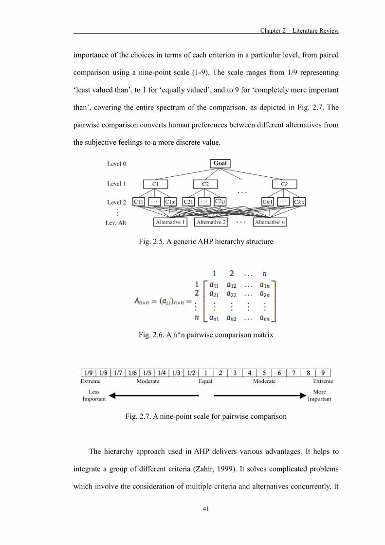
Chapter 2 – Literature Review
41
importance of the choices in terms of each criterion in a particular level, from paired
comparison using a nine-point scale (1-9). The scale ranges from 1/9 representing
‘least valued than’, to 1 for ‘equally valued’, and to 9 for ‘completely more important
than’, covering the entire spectrum of the comparison, as depicted in Fig. 2.7. The
pairwise comparison converts human preferences between different alternatives from
the subjective feelings to a more discrete value.
Fig. 2.5. A generic AHP hierarchy structure
Fig. 2.6. A n*n pairwise comparison matrix
Fig. 2.7. A nine-point scale for pairwise comparison
The hierarchy approach used in AHP delivers various advantages. It helps to
integrate a group of different criteria (Zahir, 1999). It solves complicated problems
which involve the consideration of multiple criteria and alternatives concurrently. It
Chapter 2 – Literature Review
42
has the ability to integrate data and human judgement into the model in a logical way.
Additionally, it provides a scale for measuring tangible and intangible data and for
sorting out the priorities in handling the interdependence of elements, which reduces
bias in the system (Macharis et al. 2004). This allows reconsideration of judgements
in a short period of time to monitor the consistency in the decision-maker’s judgements
so as to reduce bias in the decision making process. The ease of usage and the
conversion of subjective feelings in prioritizing alternatives makes AHP an important
part of the MCDM process.
AHP is a useful technique for decision-makers to solve complex problems. These
problems involve human perceptions and judgements on multiple criteria, which
impact on the long-term repercussions. It appears unavoidably that an organized
method of making decisions is needed. AHP has successfully gained recognition by
researchers, due to the effectiveness of the hierarchical problem identification and the
application on pairwise comparisons in preference elicitation (Salo & Hämäläinen,
1997). There is a wide range of practical applications of AHP reported, producing
extensive results in problems involving making choices, ranking, prioritization,
resource allocation, strategic planning and project management (Vargas, 1990). A
review of applications of AHP by Subramanian & Ramanathan (2012) indicated that
the decisions related to operational strategy, process and product design, planning and
scheduling resources, project management, supply chain management, were
successfully tackled by AHP. In particular, Lai et al. (2002) introduced a Multi-certeria
Authorizing System (MAS) by using the AHP technique for software selection. They
evaluated the opinions of six experienced software engineers for selecting three
products of MAS. Four hierarchy levels of pair-wise comparison were formed with
different criteria: user interface, graphical support, multi-media support, file type
support, cost effectiveness, and software maintenances. A selection consensus was

Chapter 2 – Literature Review
43
then formed by AHP and the best option for production software was selected. In the
field of project management, Al Harbi (2001) used the approach to select the best
contractor. A hierarchical structure for the pre-qualification criteria was constructed
for evaluating five contractors. The highest overall priority value was calculated after
comparing the pair-wise criteria and ranking. Furthermore, Korpela & Tuominen
(1996) presented an integrated approach to the warehouse location selection process,
where both quantitative and qualitative measures were considered. Warehouse site
selection was aimed at optimizing inventory management, and facilitating the
transportation process, as related to the design of a logistics system.
2.4.4 Genetic Algorithms
The basics of Genetic Algorithm (GA) were first introduced by Holland (1975),
and the approach has been used to successfully tackle a wide array of real-world
problems without requiring huge computation effort to retrieve an optimized solution.
Also, its flexibility allows it to be applied to various types of objective functions and
constraints in either discrete, continuous or mixed search spaces (Gen & Cheng, 2000).
The fundamental principle of the GA is to mimic the success of natural evolution
through random selection and the reproduction of offspring. Two issues must be
addressed before applying the genetic evolutionary concept to an optimization
problem: (i) encoding the potential solutions into chromosomes, and (ii) defining the
objective function, namely the fitness function. A solution (chromosomes) is encoded
in a string of variables or “genes”. The initial trial of chromosomes is randomly
generated according to certain principles or variables. The algorithm performs
evaluation to measure the fitness of the potential solutions. The procedures of the GA
mechanism are shown in Fig. 2.8. The optimization process then selects pairs of
chromosomes with probabilities proportionate to their fitness and matches them to

Chapter 2 – Literature Review
44
create new and improved solutions (offspring). In addition to matching (crossover), a
small degree of mutation is introduced to the offspring. The replacement of
underperformed solutions is based on some fixed strategies. The chromosomes which
successfully evolve through the iterations are called generations. The evaluation,
optimization and replacement of chromosomes stop when the termination criteria are
satisfied (Goldberg, 1989). The solution, which is in form of a chromosome, is then
decoded.
The genetic algorithm technique has been proven to excel in solving
combinatorial optimization problems (Ho et al., 2008). The GA operation is based on
the principles of genetic and natural evolution through random selection and the
reproduction of offspring (Renner & Ekárt, 2003; Lee et al., 2016). A nearly optimal
solution generated by the GA technique is in a form of chromosome, which involves
a string of genes. Two basic operators in GA, the crossover operator and mutation
operator, create new offspring from the parent chromosomes by selecting a pair of
chromosomes for matching, and performing a random adjustment of some values of
the genes in a chromosome, respectively. The generated chromosomes are then
evaluated through a defined fitness function. A number of GA applications have been
found in the domain of manufacturing, warehousing and distribution, showing the use
of GA for solving scheduling-related problems. Lin et al. (2014) developed a genetic
algorithm-based optimization model for managing green transportation operations.
Mendes et al. (2009) integrated GA with heuristics rules for tackling the joint
replenishment problem in warehouses. Lee et al. (2016) provided a comprehensive
quality assurance scheme in the garment industry through optimizing the fuzzy rules
using a genetic algorithm.
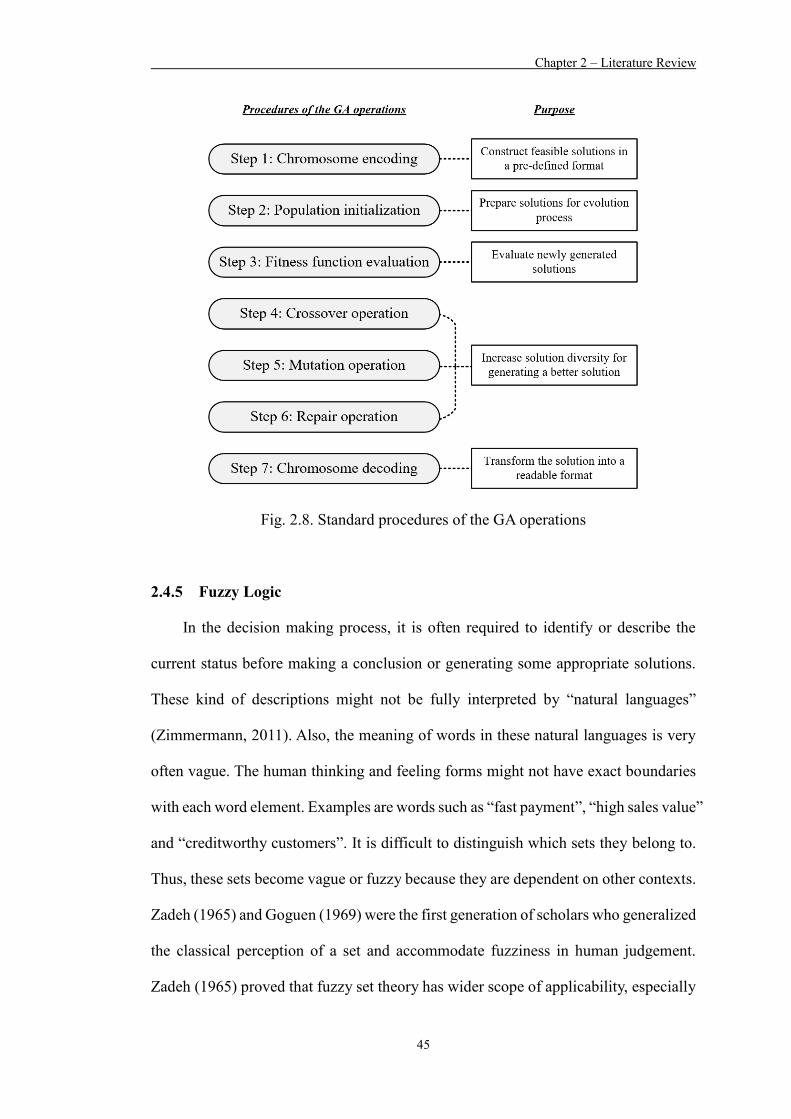
Chapter 2 – Literature Review
45
Fig. 2.8. Standard procedures of the GA operations
2.4.5 Fuzzy Logic
In the decision making process, it is often required to identify or describe the
current status before making a conclusion or generating some appropriate solutions.
These kind of descriptions might not be fully interpreted by “natural languages”
(Zimmermann, 2011). Also, the meaning of words in these natural languages is very
often vague. The human thinking and feeling forms might not have exact boundaries
with each word element. Examples are words such as “fast payment”, “high sales value”
and “creditworthy customers”. It is difficult to distinguish which sets they belong to.
Thus, these sets become vague or fuzzy because they are dependent on other contexts.
Zadeh (1965) and Goguen (1969) were the first generation of scholars who generalized
the classical perception of a set and accommodate fuzziness in human judgement.
Zadeh (1965) proved that fuzzy set theory has wider scope of applicability, especially

Chapter 2 – Literature Review
46
in the fields of data processing and pattern classification. Fuzzy set theory provides a
mathematical framework for transforming a vague concept into a precise and rigorous
numerical set which makes the decision making process more supportive. Zadeh (1978)
initiated the Fuzzy Logic technique as an artificial intelligence methodology for
simulating human reasoning (Jain et al., 2015). The ability to transform sophisticated
sentences from natural language into mathematical expressions allows fuzzy logic
technique to provide the flexibility for modeling using linguistic expressions (Jain et
al., 2015).
Fuzzy Logic is a many-valued logical method that assigns a grade of membership
between true value zero to one to each item. It is fundamentally different from Boolean
Logic as the true value of the variables of Boolean Logic can only be integer values,
i.e. zero or one, which means completely true or completely false. Instead, the true
value of variables in Fuzzy Logic can be in the range of zero to one ([0,1]), such as a
value of 0.7 (Novák et al., 2012). In early use, the most successful application of Fuzzy
Logic was in the high-speed trains in Sendai, Japan, for improving the ease and
accuracy of the ride (Kosko, 1994). Fuzzy Logic has been used in many different
aspects, such as electrical, chemical, environmental and biomedical engineering
(Singh et al, 2013).
The computing method based on fuzzy logic can be used in the development of
intelligent systems for optimization, identification, pattern recognition, control and
decision making. There are three major stages in applying the Fuzzy Logic technique:
Fuzzification, Inference engine, and Defuzzification (Siddique, 2013). The Fuzzy
Logic process starts with fuzzification. Fuzzy membership functions are defined to
address the degree of fuzziness for each parameter. To perform this fuzzification
process, the universe of discourse and membership function must be specified in order
to determine the function of the fuzzy sets. An example is illustrated in Fig. 2.9. The
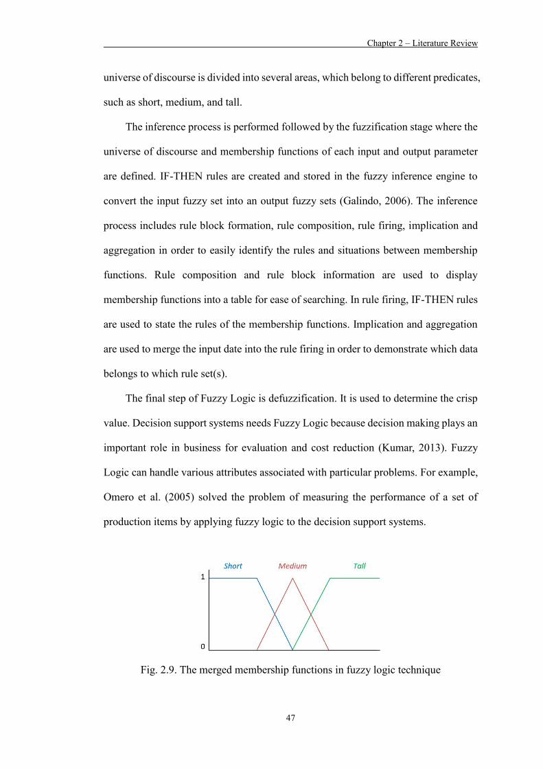
Chapter 2 – Literature Review
47
universe of discourse is divided into several areas, which belong to different predicates,
such as short, medium, and tall.
The inference process is performed followed by the fuzzification stage where the
universe of discourse and membership functions of each input and output parameter
are defined. IF-THEN rules are created and stored in the fuzzy inference engine to
convert the input fuzzy set into an output fuzzy sets (Galindo, 2006). The inference
process includes rule block formation, rule composition, rule firing, implication and
aggregation in order to easily identify the rules and situations between membership
functions. Rule composition and rule block information are used to display
membership functions into a table for ease of searching. In rule firing, IF-THEN rules
are used to state the rules of the membership functions. Implication and aggregation
are used to merge the input date into the rule firing in order to demonstrate which data
belongs to which rule set(s).
The final step of Fuzzy Logic is defuzzification. It is used to determine the crisp
value. Decision support systems needs Fuzzy Logic because decision making plays an
important role in business for evaluation and cost reduction (Kumar, 2013). Fuzzy
Logic can handle various attributes associated with particular problems. For example,
Omero et al. (2005) solved the problem of measuring the performance of a set of
production items by applying fuzzy logic to the decision support systems.
Fig. 2.9. The merged membership functions in fuzzy logic technique

Chapter 2 – Literature Review
48
2.4.6 Association Rule Mining
An association rule is a rule-based method for showing characteristic value
conditions that occur normally together in each dataset (Rajak, 2008). It provides
information in the form of “IF-THEN” statements. The rules are calculated from the
data, unlike the “IF-THEN” rules of Fuzzy Logic. Association rule mining is
probabilistic in nature, and there are two parts, the antecedent (“if”) and the consequent
(“then”) (Agrawal, 1993). An antecedent is finding an item in the data, while a
consequent is finding an item in combination with the antecedent. In association
analysis, the antecedent and consequent are called “itemsets”. There are three useful
concepts for the association rule, i.e. support, confidence and lift (Petry, 2013).
Association rule analysis has been broadly applied in various areas, such as
market analysis, medical science, and web usage mining (Rajak, 2008). It is used to
uncover specific patterns in the dataset. Also, the pattern exposes groupings of events
that occur at the same time. The most typical example of association rule mining is in
market analysis. The reason why association mining is useful for market analysis is
that it can go through numerous transaction records (e.g. 1,000,000 point-of-sale
transactions) which lists all items the customers bought in every single purchase.
Managers would like to know if certain groups of items are consistently purchased
together in order to adjust the store layout, promotions and identify customer segments
to increase the sales by attracting and bringing convenience to customers. It is a
complicated and time-consuming step if mangers do not use data mining techniques
(Mueller, 2005). In medical science, applying the association rule is an important step
in medical diagnosis and protein sequencing (Serban, 2006). The reason why it is
important in medical science is that the medical science process is complex, and the
association rule helps physicians diagnose and determine the DNA sequence by
guaranteeing the correctness of the induced hypotheses in order to improve the
Chapter 2 – Literature Review
49
prediction accuracy in complex medical applications (Gupta, 2006). Further, in the
business field, discovering association rules is an effective way that helps in decision
making and marketing (Moreno, 2005). Hence, association rule mining is useful for
analyzing customer behavior and background.
2.4.7 Adaptive Network-Based Fuzzy Inference System
ANFIS is a fuzzy inference system implemented in the framework of adaptive
networks, indicating that the fuzzy inference system is based on neural networks (Jang,
1993). Similar to ANN, ANFIS has a capability of modeling linear and nonlinear
functions (Jang et al., 1997).
ANFIS is comprised of fuzzy inference system and adaptive neural network as
the major elements. For the fuzzy inference system (FIS), it is based on the fuzzy “If-
Then” rules for human knowledge and inference procedures to perform qualitative
description and analysis, except for the lack of accurate quantitative analysis and
correction of values (Su & Cheng, 2016). ANFIS is used to link the input
characteristics to input membership function (MFs), input MFs to a set of If-Then rules,
the set of rules to output characteristics, output characteristics to output MFs and
finally to the single-valued output or the decision associated with the output. For the
adaptive network of ANFIS, it is a network structure consisting of a number of nodes
connected through directional links. The outputs of these adaptive nodes depend on
modifiable parameters pertaining to these nodes. The learning rule specifies how these
parameters should be updated to minimize error (Güneri et al., 2011). Details for
fundamental principles of ANFIS are published elsewhere (Jang, 1993, Jang et al.,
1997,), so detailed descriptions of these methods are not given here. The theoretical
rationale of the ANFIS models proposed in this study is discussed in Section 3.6.2 –
ANFIS Model Construction.

Chapter 2 – Literature Review
50
ANFIS has been widely used in solving different sorts of problems. In the
literature, researchers apply the hybrid learning structure of ANFIS for performance
comparison with other neural network oriented studies (Lee, 2008; Shiri et al., 2011;
Areerachakul, 2012; Alrashed wt al., 2018). Polat and Güneş (2007) used principal
component analysis and ANFIS to improve the diagnostic accuracy in diabetes disease.
The dimension of the diabetes disease dataset that has 8 features is reduced to 4
features using principal component analysis, followed by a diagnosis of diabetes
disease through using an adaptive neuro-fuzzy inference system classifier, which is
able to give a 89% of classification accuracy. In the context of supply chain
management, researchers applied ANFIS models for tackling common problems
addressed in the literature, such as supplier selection and evaluation of supply chain
performance. Güneri et al. (2011) proposed an ANFIS-based approach to deal with
supplier selection problem by applying the ANFIS model for selecting supplier
selection criteria. The results revealed a better performance by the developed ANFIS
model over the multiple regression method in selecting the criteria for supplier
selection. Didehkhani et al. (2009) developed a supply chain flexibility assessment
model using ANFIS through taking flexibility attributes, such as operation, new
product and responsiveness, into the modelling of the ANFIS model.
In general, ANFIS models have a diverse area of applications in the literature,
with a number of studies adopting ANFIS for tackling a forecasting problem. These
studies suggest that the integration of the fuzzy inference system and adaptive neural
network in ANFIS is capable of modeling linear and non-linear functons and
predicting a subject well. For the studies using ANFIS for solving forecasting
problems, a review and discussion is given in section 2.5.2.2 – ANFIS-based
Forecasting Model.
Chapter 2 – Literature Review
51
2.5 Existing Approaches for Time-series Data Prediction
2.5.1 Stochastic Modelling for Time Series Data Prediction
Stochastic time series models for time series demand forecasting, such as moving
average (MA), autoregressive moving average (ARMA), and autoregressive
integrated moving average (ARIMA), have been widely applied in various areas in the
past few decades. These methods assume that the time series is linear and follows a
particular known statistical distribution. The high dependency on historical data of
these time series models limits their applicability, as real data can be incomplete,
imprecise, and given in linguistic values. However, stochastic time series models are
still perceived to be essential tools for forecasting time series data. This section
discusses some popular stochastic time series forecasting tools, including: linear
regression, moving average, exponential smoothing, auto regressive and
autoregressive integrated moving average model.
2.5.1.1 Linear Regression Model
Linear regression is a prediction technique that involves the extent to which the
independent variables can predict the dependent variable (Hair et al., 2010). It is a
statistical method that can summarize and study the relationship between two
continuous variables x and y. Variable x is a predictor or independent variable while y
is a response or dependent variable. It is assumed that the relationships between
variables are linear, of two basic type: simple linear regression (SLR) and multiple
linear regression (MLB).

Chapter 2 – Literature Review
52
Simple linear regression (SLR)
Simple linear regression (SLR) is a linear regression model with a single
explanatory variable (Seltman, 2008). SLR forecasting models are expressed as
Eq. 1:
𝑌𝑡 = 𝑏0 + 𝑏1𝑥𝑡 + 𝜀𝑡 (1)
where Yt is the dependent variable and predicted value of Y at time t, b0 is the
estimation of regression intercept, b1 is the estimation of the regression slope and
xt is the independent variable and value of x at time t. ε is the individual error term
which has a mean of zero.
Multiple linear regression (MLR)
Multiple linear regression (MLR) is used to examine the linear relationship
between a single dependent variable and two of more independent variables.
MLR forecasting models are expressed as Eq. 2:
𝑌𝑡 = 𝑥𝑡𝛽 + 𝜀𝑡 (2)
where Yt is the dependent variable and predicted value of Y at time t, xt is the
vector of k explanatory variables at time t, i.e. xt = 1, xi1, x2t, …, xkt. β represents
the vector of coefficient, i.e. β= (β0, β1, …, βk)T and εt is the individual error term
at time t, i.e. t = 1, 2, …, N.
Linear regression is a technique that fits a trend equation or a curve to a series of
historical data points and projects the curve into the future for medium and long term

Chapter 2 – Literature Review
53
forecasts. It has been widely used to measure the strength of the relationship between
independent and dependent variables. Bartosz (2014) proposed the use of Simple
Linear Regression and Multivariate Adaptive Regression Splines to estimate the share
returns on the Warsaw Stock Exchange. Lin & Tsai (2015) used a simple linear
regression approach for forecasting mortality rates. Bas et al. (2017) proposed a
multiple linear regression model and a SARIMA model for air concentration
forecasting. Latt & Hartmut (2014) used stepwise multiple linear regression (SMLR)
and artificial neural network (ANN) models as tools for multi-step forecasting of the
Chindwin River floods in northern Myanmar.
2.5.1.2 Moving Average (MA) Model
The moving average method is one of the time series analysis techniques used
for smoothing short period fluctuations, showing the trend by generating the weighted
average of the past period observation (Lauren & Harlili, 2014). There are two types
of moving average: simple moving average (SMA) and weighted moving average
(WMA).
Simple moving average
Simple Moving Average is the average demand of a number of periods that is
used for forecasting the next period. It is used for stable demand with no
pronounced behavioral pattern, and is calculated by Eq. (3).
𝑆𝑀𝐴𝑛 =∑ 𝐷𝑖
𝑛𝑖=1
𝑛 (3)
Chapter 2 – Literature Review
54
where SMAn is the forecasted rate for period n, Di represents the demand for the
period and n denotes to the number of periods considered in the moving average
calculation.
Weighted Moving Average
Weighted Moving Average is the adjusted moving average method that more
closely reflects data fluctuations. It can modify the technique to give greater
weight to a more recent observation. It is calculated by Eq (4).
𝑊𝑀𝐴𝑛 = ∑ 𝑊𝑖𝐷𝑖𝑛𝑖=1 (4)
where WMAn is the forecasted rate for n period, Di represents the demand for the
period, Wi represents the weighting of period i which between 0% and 100% and
n responses to the number of periods in the moving average.
The moving average predicts the trend of the data. It is simple and more effective
than other comparably more complex techniques (Lauren & Harlili, 2014). MA can
avoid noise and therefore smoothing of the trend environment. There are short-term
moving average and long-term moving average. If the value of short-term moving
average is greater than the long-term simple moving average, an up-going trend is
indicated. On contrary, the reverse occurs.
There are many factors affecting the prediction of the time series data. Due to the
simplicity of MA, it is rarely used independently. It is combined with other factors or
algorithms in particular aspects. For stock trend prediction, Lauren & Harlili (2014)
proposed the combination of the simple moving average and news classification by
artificial neural network (ANN). Sulandari & Yudhanto (2015) proposed a hybrid

Chapter 2 – Literature Review
55
approach of moving average and weighted fuzzy time series to enhance the forecasting
accuracy in the trend data. For environmental forecasting, Fhira et al. (2015) suggested
using MA to smooth the rainfall time series data and observe the input vector for the
prediction process by using an Evolving Neural Network. It shows that although MA
is rarely used independently, it can be integrated with other prediction methods for
conducting the prediction.
2.5.1.3 Exponential Smoothing Model
The exponential smoothing model is a powerful tool for forecasting future
demand and is one of the moving average methods. (Liljana et al., 2016; Su et al.,
2018). Exponential smoothing generates forecasting by weighting the averages of past
observation and giving the recent values a relatively more weight than the older
observation in forecasting (Makridakis et al., 1998; Su et ai, 2018). Past data is rejected
gradually rather than suddenly. Holt (1975) and Brown (1959 &1963) introduced the
single exponential smoothing of time series data and extended by Holt to linear
exponential smoothing to enable forecasting of the data with trends. Exponential
smoothing assumes that time series are built from unobserved components such as
trend and seasonal effects. Those components have been adapted over time to follow
the demand pattern (Billah et al., 2006). The formula of exponential smoothing is:
𝐹𝑡+1 = 𝛼𝐷𝑡 + (1 − 𝛼)𝐹𝑡 (5)
where Ft+1 is the forecast for next period, Dt represents the actual demand for the
current period, Ft refers to the previously determined forecast for current period and
𝛼 is the weighing factor, a smoothing constant between 0 and 1. If great variation in
a short period is observed, a small value of the smoothing constant should be selected.

Chapter 2 – Literature Review
56
On the contrary, the high value of the smoothing constant should be selected. The
greater the variation observed, the smaller value of the smoothing constant to be
selected.
Exponential Smoothing can predict the data with the trend. It is suitable for
forecasting the short-term and medium-term time periods with good accuracy
compared with other algorithms. Due to its simplicity, the forecasting method is
comparable to forecasts of more complex statistical time series data (Makridakis and
Hibon, 2000). Exponential smoothing is widely used in forecasting the data with the
trend. In an environmental application, Su et al. (2018) proposed exponential
smoothing for forecasting the water ecological footprint (WEF) as well as defining the
future trends of WEF. In the field of logistics, Liljana et al. (2016) developed a
smoothing method for forecasting the time series data with several zero entries and
substantial noise, with the Holt-Winters smoothing methods introduced. Taylor (2011)
proposed an exponential smoothing based model for forecasting the density of
intraday call center arrivals. It shows that exponential smoothing can be widely used
in different applications and is appropriate for forecasting the data with the trend.
2.5.1.4 Auto Regressive (AR) Model
An autoregressive model is a linear regression of the current value of the series
against one or more prior values of the series (Wei et al., 2014). The AR model
includes one or more past values of the dependent variable among its explanatory
variables. The autoregressive moving average model (ARMA) is a conventional
method which is applicable to forecast regular periodic data, such as seasonal or
cyclical time series data. It is a statistical approach that enables modelling the time
series and predicting time series data behavior (Flores et al., 2012). Box and Jenkins
(1976) developed a general linear stochastics model by assuming random shocks.

Chapter 2 – Literature Review
57
An AR model is used when a value from a time series is regressed on a previous
value from that same time-series data, i.e. yt on yt-1. The order of the AR is the number
of immediately preceding value in the series that are used to predict the value at the
present time. For first-order autoregression, the model can be expressed as Eq. 6.
AR (1):
𝑦𝑡 = ∅1𝑦𝑡−1 + 𝜇 + 𝜐𝑡 (6)
where 𝜐𝑡 is the white noise viewed as a random error, 𝜇 represents the constant term
and ∅1 is the first-order autoregression coefficient. It can be thought of as that for a
given value y in time period t that has a relationship with time period t+1. For p order
autoregression, the autoregressive model can be expressed as Eq. 7.
AR (p):
𝑦𝑡 = 𝜇 + ∅1𝑦𝑡−1 + ∅2𝑦𝑡−2 + ⋯ + ∅𝑝𝑦𝑡−𝑝 + 𝜐𝑡 (7)
The AR model is used to describe certain time-varying processes. It specifies that
the output variable linearly depends on its own previous values and on an imperfectly
predictable term. AR is not always stationary as it may contain a unit root. AR can be
combined with other time series forecasting models such as the moving average.
Kristiansen (2012) proposed an autoregressive model with exogenous variables to
predict the price. Othman et al. (2015) suggested an HAR model which combined the
Hammerstein model to an Auto-Regressive approach to forecast recursive wind speed,
and it was found that the HAR model had a better performance compared with ARIMA
and ANN in terms of the prediction accuracy. Yu et al. (2014) developed a hybrid
model combining the seasonal auto-regressive integrated moving average (ARIMA)

Chapter 2 – Literature Review
58
model and the nonlinear auto-regressive neural network to forecast the expected
incidence cases of hand-foot-mouth disease in Shenzhen, China.
2.5.1.5 Autoregressive Integrated Moving Average (ARIMA) Model
The ARIMA model is a statistical technique for time series prediction that was
proposed by Box–Jenkins in 1970 (Box et al., 2008). The ARIMA is one of the most
popular time series forecasting analysis approaches that originated from the
autoregressive model (AR), the moving average model (MA) and the combination of
the ARMA models (Ho et al., 2002). It can be used when the time series data is
stationary and there are no missing data within the time series. ARIMA generates an
identified underlying process based on observations to a time series for generating a
good model that shows the process-generating mechanism precisely (Box and Jenkins,
1976). The ARIMA technique includes identification, estimation and diagnostic
checking (Abdel-Aal &Al Garni, 1997). A non-seasonal ARIMA model is classified
as an ARIMA (p, d, q) model and expressed as shown in Eq. 8, where p represents the
number of autoregressive term, d represents the number of non-seasonal differences
needed for stationary and q is the number of lagged forecast errors in the predicted
equation.
𝑌𝑡 = μ + ∅1𝑦𝑡−1 + ⋯ + ∅𝑝𝑦𝑡−𝑝 − 𝜃1𝑒𝑡−1 − ⋯ − 𝜃𝑞𝑒𝑡−𝑞 (8)
where y is the dth difference of Y. For d =1, yt = Yt + Yt-1. For d =2, yt = (Yt + Yt-1) -
(Yt-1 + Yt-2). The second difference of Y indicates the first difference of the first
difference, which is discrete analog of the second derivative. θ represents the
moving average parameter. Hence, ARIMA (0,1,1) with a constant value means simple
exponential smoothing. The seasonal components which are determined where the
Chapter 2 – Literature Review
59
autocorrelation functions cut the confidence limits, can be included in the ARIMA
model and is called SARIMA.
ARIMA is a sophisticated forecasting method as it combines the features of all
other methods. It is not required to choose the initial values of any variable and the
values of various parameters a priori. ARIMA can reduce a non-stationary series to a
stationary series using a sequence of differencing steps and can determine the best-fit
model for the respective time series (Sen et al. 2016). Its flexibility and orderly
searching at each stage takes advantage by comparing with other forecasting methods.
When the time series is stationary and data is complete, the ARIMA model can be used
in the time series.
ARIMA has a wide range of applications in forecasting time series data. Edigera
and Akar (2007) proposed the usage of the Integrated Moving Average (ARIMA) and
seasonal ARIMA (SARIMA) methods to estimate the future primary energy demand
of Turkey. Arunraj & Ahrens (2015) suggested the usage of hybrid seasonal
autoregressive integrated moving average and quantile regression for daily food sales
forecasting. Jiang et al (2018) used ARIMA for forecasting China’s coal consumption,
price and investment by 2030. Mohamed and Bodger (2005) considered the ARIMA
model to forecast the electricity consumption in the eastern part of Saudi Arabia and
Lebanon.
ARIMA models are flexible as they are able to represent several different types
of time series, such as pure autoregressive (AR), pure moving average (MA) and
combined AR and MA (ARMA) series. However, Zhang (2003) suggested that the
pre-assumed linearity of ARIMA models is a major bottleneck in using ARIMA
models to forecast real-life problems. The approximation of linear models to complex
real-world problem is not always satisfactory. Therefore, formally specifying and
assuming the linearity characteristics and a probability distribution for time series data

Chapter 2 – Literature Review
60
makes the development and deployment of this type of linear time series model
difficult (Hansen et al., 1999).
2.5.2 Machine Learning Techniques for Time Series Data Prediction
For more than half a century, ARIMA models dominated many areas of time
series forecasting. In recent times, machine learning techniques, particularly Artificial
Neural Network-based and ANFIS-based models, have become widely adopted for
time series data forecasting. The application of these techniques suggest that there may
be more accurate time series forecasting models other than the conventional stochastic
linear time series models, such as MLR, ARMA and ARIMA models, as introduced in
the previous section. Therefore, the applicability of Artificial Neural Network-based
and ANFIS-based models in forecasting time-series models are discussed in the
following sections.
2.5.2.1 Artificial Neural Network-based Forecasting Model
ANN can be defined as an information processing system whose structure and
functioning are inspired by biological neural networks. They have three fundamental
features: parallel processing, distributed memory and adaptability. Such features
enable ANN to outperform other processing systems in terms of robustness and a
tolerance to error and noise (Palmer et al., 2006). ANNs are universal function
approximators capable of mapping any linear or non-linear function (Cybenko, 1989;
Funahashi, 1989). They are able to approximate a large class of functions with a high
degree of accuracy, attributed to the ability of parallel information processing from the
data (Zhang, 2003). For this reason, the study of artificial neural networks (ANN) has
aroused great interest in fields as diverse as biology, economics, mathematics,
statistics and computers (Palmer et al., 2006).

Chapter 2 – Literature Review
61
In general, an ANN is a network model made up of a large number of simple
processing elements, which are known as nodes or neurons. In the network, these
neurons, which are organized in several layers, are inter-connected to other neurons
by communication links, with each link associated with a numerical value known as
“weight”. The network structure of an ANN is largely determined by the
characteristics of the data, and no pre-assumption of the form of the model is required
in the model building process. Due to the capability of solving a wide variety of
problems, single hidden layer feedforward network is the most widely applied model
form of ANN for time series modeling and forecasting (Kaastra & Boyd, 1996; Zhang,
Patuwo & Hu, 1998). The model, as discussed by Zhang (2003), is characterized by a
network of three layers of simple processing units. The relationship between the output
(yt) and the inputs (yt−1,yt−2,…,yt−p) can be expressed by the following equations:
𝑦𝑡 = 𝛼0 + ∑ 𝛼𝑗𝑔(𝛽0𝑗 + ∑ 𝛽𝑖𝑗𝑦𝑡−𝑖) + 𝜀𝑡𝑝𝑖=1
𝑞𝑗=1 (9)
where αj, for j = 0, 1, 2, …., q and βij, for i = 0, 1, 2, …., p, and j = 0, 1, 2, …., q, are
the model parameters known as “weight”, containing the knowledge that ANN possess
about a specific problem; p and q respectively denotes the number of input nodes and
hidden nodes. A logistic function is often used as the hidden layer transfer function,
that is,
g(x) = 1
1+exp (−𝑥) (10)
With the ANN model mathematically expressed in (x), the model is equivalent to
a nonlinear autoregressive model that maps the past observations, i.e. yt-1, yt-2, …, yt-p

Chapter 2 – Literature Review
62
to the predicted value yt. As ANN has been found to be a viable contender to various
traditional time series models (Giordano et al., 2007, Jain & Kumar, 2007), the
application of ANN can be found across a variety of fields, such as marketing and
segmentation analysis (Dolnicar & Fluker, 2003; Cho, 2003; Bloom, 2005), demand
forecasting in environmental aspects (Neto & Fiorelli, 2008; Kaytez et al., 2015;
Ahmad et al., 2017; Lee et al., 1992), forecasting problems in supply chain
management (Kochak & Sharma, 2015; Jaipuria & Mahapatra, 2014).
2.5.2.2 ANFIS-based Forecasting Model
Fuzzy forecasting approaches are capable of dealing with vague and incomplete
time series data under uncertain circumstances (Egrioglu et al., 2011; Lu et al., 2014;
Dombi et al., 2018). The adaptive neuro-fuzzy inference system (ANFIS), a fuzzy
Sugeno model integrated into the framework of adaptive systems to facilitate machine
learning and adaption using testing data sets (Jang, 1993), is one of the popular fuzzy
approaches for forecast modelling. It combines the advantages of the neural network
and fuzzy systems, thereby being more flexible, adaptive and effective on highly non-
linear complex problems among other fuzzy inference systems (Kar et al., 2014). The
ANFIS creates its own structure and can serve as a basis for constructing fuzzy if–then
rules with appropriate membership functions so as to generate the stipulated input–
output pairs (Admuthe & Apte, 2010). The self-learning ability of ANFIS makes it less
reliant on human knowledge and experience for making wise decisions (Übeyli &
Güler, 2006). ANFIS has been established as one of the most popular approaches for
making accurate forecasting. Researchers have successfully applied ANFIS to a
variety of areas in the past decades. ANFIS can improve the uncertainty of the model
and the imprecision of the system. Its self-learning ability to learn through data sets
and the organizational capacity is able to adjust the parameters of the model (Su &

Chapter 2 – Literature Review
63
Cheng, 2016). In comparing with other forecasting models, ANFIS has a high speed
of training, and the most effective learning algorithm (Jang et al., 1997). Moreover,
ANFIS is the best function approximator among the several neuro-fuzzy models and
is faster in convergence in comparion with others neuro-fuzzy models (Akcayol, 2004).
It provides the best result when applied without any pretraining (Altug et al., 1999).
Therefore, ANFIS is appropriate for forecasting time series data when compared with
other models.
In recent years, the ANFIS system has been widely used for forecasting nonlinear
models of processes to determine the input-output relationships in many areas. In the
stock market, Wei et al. (2014) and Su & Cheng (2016) proposed the forecasting of
stock using a hybrid ANFIS model. Due to the complex factors and nonlinear
relationship between those factors existing in different periods, forecasting in the stock
market is difficult. The ANFIS forecasting method was proposed to forecast stock
prices in order to eliminate the drawback of other forecasting methods. In the
environmental aspects, Sinvaldo et al. (2018) proposed a hybrid SSA-ANFIS-FCM
approach for wind speed forecasting. The hybrid model can learn the trend and the
wind time series structure. The prediction errors were significantly decreased by
applying the proposed technique. Prasad et al. (2016) suggested an ANFIS model in
forecasting the air pollution concentration of five air pollutants (sulphur dioxide,
nitrogen dioxide, carbon monoxide, ozone and particulate matter). In the logistics
aspect, Wang and Chen (2008) suggested rush order control application by applying
the neuro-fuzzy based forecasting approach. The proposed model solves the problem
of predicting rush orders for regulating the capacity reservation mechanism in advance.
Popular areas of ANFIS forecasting applications include the stock market
(Guresen et al., 2011; Esfahanipour & Aghamiri, 2010; Svalina et al., 2013),
environmental-related aspects and energy consumption prediction (Khoshnevisan et

Chapter 2 – Literature Review
64
al., 2014; Zahedi et al., 2013), weather forecast (El-Shafie et al., 2011; Osório et al.,
2015), and demand forecast in various industries (Wang et al., 2011; Xiao et al., 2014;
Nilashi et al., 2011). However, the application of ANFIS in the field of order
management in the retail and logistics sector is rarely found. Wang and Chen (2008)
applied ANFIS to forecast product items, quantities and the occurance of contingent
rush orders in a manufacturing firm. Aengchuan and Phruksaphanrat (2018) compared
the fuzzy inference system (FIS), FIS with artificial neural networks (FIS+ANN) and
FIS with adaptive neuro-fuzzy inference system (FIS+ANFIS) for inventory control.
This research extends the application area of ANFIS in the literature by proposing an
ANFIS with the integration of the autoregressive (AR) model for the prediction of e-
commerce logistics order arrival in distribution centres. Through the prediction of the
arrival pattern of e-orders, logistics practitioners are able to wisely allocate resources
in advance, and consolidate discrete, fragmented e-commerce orders prior to actual
batch processing of consolidated orders in distribution centres, so as to improve the
order handling capability and supply chain efficiency especially in the complex and
dynamic e-commerce operating environment.
2.6 Summary
Logistics practitioners have been facing enormous challenges in the order
fulfillment process under the emerging e-commerce operating environment. The
reason behind the difficulty in handing e-commerce orders lies in the fact that most
practitioners are still sticking with the conventional order processing flow to handle e-
commerce orders, i.e. perform order handling operations in warehouses immediately
upon receiving an order delivery instruction by the customers, such as retailers and
wholesalers. However, in today’s e-commerce business environment, orders are
placed by the end consumers at anytime. Immediate order handling of one single e-

Chapter 2 – Literature Review
65
commerce order is illogical and irrational. In the literature, studies that focus on
improving the operating efficiency in e-fulfillment distribution centres have been
lacking. Most studies in the past decade attempt to tackle specific cases, settings or
scenarios in the warehouse, without a focus of the e-commerce order handling
bottlenecks that lead to a serious order handling inefficiency.
To this end, this study proposes the need to re-engineer the e-order fulfilment
process by grouping e-orders for batch processing. To effectively deal with e-orders
for bulk order handling, two essential factors must be carefully considered, i.e. how
they are grouped and when they should be released (“When to release”) for batch
processing in distribution centres. To provide decision support for these issues, this
research integrates GA and ANFIS to respectively group e-orders and determine the
timing for a batch release of e-orders. As the “When to release” decision is concerned
with forecasting the arrival of e-orders, conventional stochastics times series models
and machine learning models for time series data forecasting are also thoroughly
reviewed in this chapter. It is suggested that improving time series forecasting
accuracy is an important yet often difficult task facing forecasters. Moreover,
assuming the e-order arrival data to have linear characteristics and follow a probability
distribution is not justifiable. Therefore, a hybrid methodology that integrates the
elements of ARIMA into the construction process of ANFIS models, is proposed to
take advantage of the unique strength of ARIMA and ANN models in linear and
nonlinear modeling. Past observations of the same variable are collected and analyzed
to develop a model for describing the underlying relationship.

Chapter 3 – An E-commerce Fulfillment Decision Support System (EF-DSS)
66
Chapter 3 – An E-commerce Fulfillment Decision Support System
(EF-DSS)
3.1 Introduction
In this chapter, the design of the E-commerce Fulfilment Decision System (EF-
DSS) is presented. The EF-DSS is designed with an aim of re-engineering of the e-
commerce order processing flow in distribution centres. This objective is achieved by
applying the “Warehouse Postponement Strategy” (WPS) to group fragmented,
discrete and small lot-sized e-commerce orders before releasing the consolidated e-
orders in a batch for processing these orders at the same time. To better illustrate the
need to implement WPS, this chapter begins with an introduction of the WPS proposed
in this research study in Section 3.2, followed by a comprehensive discussion of the
architecture and the elements involved in the EF-DSS in Section 3.3. The E-order
consolidation module (ECM) of the EF-DSS, which serves as the consolidation pool
of e-commerce orders, is presented in Section 3.4. The E-order grouping module
(EGM) of the EF-DSS, which integrates a GA-based algorithm for grouping e-
commerce orders with similar attributes, is introduced in Section 3.5. Lastly, the E-
order batch releasing module (EBRM) that determines the timing for releasing the
grouped e-orders through the prediction of the arrival rate of e-commerce orders in the
coming time periods using multiple novel Autoregressive-momentum-moving
average-based adaptive neuro-fuzzy inference system (AR-MO-MA-ANFIS) models,
is discussed in Section 3.6.
Chapter 3 – An E-commerce Fulfillment Decision Support System (EF-DSS)
67
3.2 The Concept of Warehouse Postponement Strategy
Why WPS is needed?
The rapid growth of the e-commerce market around the globe over the last decade
has drastically revamped the retail industry. End-consumers are not only able to
purchase goods at local physical stores, but also from online shops from any corner of
the world. According to market research conducted by Statista Inc. (2015), over 40
percent of global internet users purchased products online in 2013. In 2018, this figure
is expected to edge close to 50 percent of internet users worldwide (Statista Inc., 2015),
showing the growing trend of delivering online-to-offline (O2O) shopping experience
to consumers. Due to the changing consumer purchasing behavior, as well as the
environment in the retail industry, logistics practitioners are capturing e-commerce
logistics markets while improving their capability and capacity of handling such e-
commerce business. On the technical side, for example, logistics service providers
provide real-time order tracking capability for realizing supply chain information
transparency.
The boundary spanning of logistics service providers (LSPs), however, is never
easy to accomplish. The transformation of their core businesses into integrated e-
commerce logistics solution provision is formidable, owing to the fact that operational
capability could very probably be the major obstacle to face. While cross-border e-
commerce and O2O business is a huge market opportunity for logistics practitioners
around the world such as third-party logistics service providers and freight forwarders,
they have been facing fundamental challenges in complying with the ever increasing
and challenging needs of providing proper logistics and supply chain solutions for e-
commerce businesses.
Conventionally, in the absence of O2O and e-commerce business models,
consumers purchase items solely at physical retail stores. In this sense, LSPs handle

Chapter 3 – An E-commerce Fulfillment Decision Support System (EF-DSS)
68
goods in bulk for delivery to wholesalers or retailers, usually on a weekly or bi-weekly
basis, primarily for stock replenishment. However, with the presence of online
shopping platforms which enable customers to purchase online, LSPs are required to
handle a large number of stock-keeping units (SKUs), pick and pack small volume
orders and deliver them in small parcel shipments to end consumers with tighter
schedules. Therefore, the traditional order fulfillment process in warehouses and
distribution centers (DC) that encompasses receiving, put-away, picking and transport
of goods in bulk, is unable to fulfill the order handling requirements of e-commerce
shipments. The fundamental differences between traditional order handling and e-
commerce order handling could well explain why e-commerce businesses have had
serious challenges to the efficiency of the last-mile of e-commerce fulfillment, and
have been reshaping the position and degree of importance of LSPs along the supply
chains.
In view of the increasing concern over the order fulfillment performance of LSPs
in the e-commerce business environment, Warehouse Postponement Strategy (WPS),
a process-oriented tactic addressing logistics process postponement in warehouses and
DCs, is conceptualized and proposed. Such a strategy enables logistics practitioners to
cope with e-commerce order handling requirements through streamlining order
handling procedures. Ultimately, it enables operations to align with the strategic
directions in integrating e-commerce logistics businesses.
The Definition of WPS
Postponement, also called delayed differentiation, is a widely accepted tactic for
dealing with uncertainties and fluctuations in demand, delays the customization and
final assembling of products (Yang et al., 2004). It has been recognized as an effective
strategy to manage uncertainties and variability in demand. Zinn and Bowersox (1988)

Chapter 3 – An E-commerce Fulfillment Decision Support System (EF-DSS)
69
identified five deferral strategies, four of which related to changes in the product,
including labeling, packaging, assembling, and manufacturing. The remaining
postponement strategy focuses on logistics postponement, that is, (i) place
postponement – the storage of finished products in centralized logistics systems, and
(ii) time postponement – a time delay for slowing the movement of the product until
the last possible moment, rather than responding rapidly to customer demand.
With the intensified challenges of managing a global supply chain that is
responsive to customer demand in today’s long-tail market, the concept of
postponement strategy has been noted as a viable solution in the face of increasing
product variety, shorter product lifecycle, and faster response to customer needs
(Twede et al., 2000; Boone et al., 2007; Yang et al., 2004; Yang and Yang, 2010; Choi
et al., 2012). It has been researched as an essential topic in the production and
inventory management literature (Lee and Tang, 1997; Pagh and Cooper, 1998; Yang
et al., 2004). While postponement strategy in supply chains is widely recognized as an
indispensable means of dealing with the risk pooling effect through properly managing
the inventory for meeting unavoidable demand uncertainties, the focus of conventional
postponement strategy is on how the configuration and assembling of a product can
be delayed until the last possible moment.
When the concept of conventional postponement strategy is introduced at the
warehouse operational level, it would be beneficial for logistics practitioners to
manage discrete, fragmented and small lot-sized e-commerce orders under today’s
dynamic and complex e-commerce and O2O logistics operating environment. The
proposed Warehouse Postponement Strategy (WPS) is transformed from the concept
of conventional product-oriented supply chain postponement strategy. It is defined as
“an operation strategy to delay the execution of a logistics process until the last
possible moment”. Considering the receiving, storage, picking and shipping

Chapter 3 – An E-commerce Fulfillment Decision Support System (EF-DSS)
70
operaitons as the four typical categories of warehousing activities (Berg & Zijm, 1999),
the implementation of WPS in warehouses allows the postponement of performing the
next category of warehouse operation. Fig. 3.1 illustrates a before and after
comparison of WPS in warehouses and distribution centers. Without the introduction
of WPS, orders received from customers directly initiate the order processing
procedures in a warehouse. The warehouse order throughput rate fluctuates throughout
the working hours and is dependent on the actual number of orders received
throughout the day. In this sense, taking order pick-and-pack operation as an example,
warehouses operators are required to repeatedly visit the storage locations to pick the
goods for fulfilling the orders throughout the whole day. The efficiency is therefore
heavily affected by the absence of postponing or grouping outstanding orders for batch
or wave processing.
With the introduction of WPS, operators no longer perform warehouse operations
solely based on the immediate order they have just received. Instead, a pre-process
order pool, as illustrated in Fig. 3.1, allows logistics practitioners to configure the cut-
off time and amount in order to postpone the order processing operations until the “last
possible moment”. Upon reaching the pre-defined cut-off criteria, grouped outstanding
orders are released to the warehouse for batch process execution. Therefore, the
throughput rate in a warehouse would follow a wave pattern instead of a fluctuating
one. The rearranged throughput rate then derives several benefits in aspects such as
order handling efficiency, resource management and workforce level adjustment.
However, the cut-off criterion is not a straightforward decision to make, in the
absence of IT or artificial intelligence techniques, aiding decision support. Without
these decision support tools, logistics practitioners rely on their previous experience
and practice to determine the “optimal” cut-off point, which is very often unable to

Chapter 3 – An E-commerce Fulfillment Decision Support System (EF-DSS)
71
meet the fast changing warehouses and distribution center environment particularly in
today’s e-commerce logistics business environment.
Fig. 3.1. Order throughput difference with and without the application of WPS
3.3 Architecture of the EF-DSS
Effective deployment of Warehouse Postponement Strategy requires making
accurate decisions regarding: (i) How to group the e-commerce orders, and (ii) when
to release the grouped e-commerce orders. Therefore, the EF-DSS is designed to
provide decision support as to how the e-orders are grouped and when they should be
released in batch, so as to realize the concept of Warehouse Postponement Strategy for
facilitating LSPs in managing today’s e-commerce logistics orders. The architecture
of EF-DSS, as shown in Fig. 3.2, consists of three modules: E-order consolidation
module (ECM), E-order grouping module (EGM), and E-order batch releasing module
(EBRM).
Chapter 3 – An E-commerce Fulfillment Decision Support System (EF-DSS)
72
In the ECM, there is a centralized database to gather and store data, such as e-
commerce order information, customer profiles, and resource status in distribution
centres. To deploy the proposed warehouse postponement strategy, e-commerce orders
received by the logistics service providers have to be grouped before batch releasing
to the distribution centres for processing in batch. The grouping and consolidation of
pending e-commerce orders is achieved by an e-order consolidation pool built in the
ECM of the EF-DSS. Other relevant information collected and stored in the database
of ECM is then used for generating and extracting useful decision support in the next
module of the EF-DSS.
In the EGM, data stored in the centralized database in the ECM are processed and
serve as the inputs of this module to determine “How to group” the pending e-
commerce orders. Ordered items, which are pending in the e-order consolidation pool
of the ECM, are grouped based on the proximity of storage locations using a genetic
algorithm approach. In other words, items with similar storage locations in the
distribution centres or warehouses are grouped together for batch order picking. By
grouping the pending ordered items in several batches using the GA, the order pickers
in the distribution centres are able to perform batch order picking operations for the
discrete, fragmented e-commerce orders.
Though the EGM provides decision support for the logistics service providers to
effectively group the e-orders for batch order picking operations, the logistics service
providers still have to decide the cut-off time or quantity to stop consolidation of the
e-commerce orders. In this respect, the EF-DSS further suggests the cut-off time based
on a prediction of the e-order arrival frequency in the upcoming period using a novel
autoregressive-based Adaptive Network-Based Fuzzy Inference System (AR-ANFIS)
approach. Hence, the logistics service providers are able to identify how much time
can they still consolidate the incoming e-commerce orders. Once the cut-off time

Chapter 3 – An E-commerce Fulfillment Decision Support System (EF-DSS)
73
Fig. 3.2. Architecture of the EF-DSS

Chapter 3 – An E-commerce Fulfillment Decision Support System (EF-DSS)
74
has been reached, the pending e-orders are grouped in several batches based on their
storage location proximity. Therefore, the proposed warehouse postponement strategy
can effectively be deployed with essential decision support provided by the EF-DSS.
Details of each module are presented in the following sections.
3.4 E-order consolidation module (ECM)
In the era of the e-commerce business, delivery orders placed by end consumers
are retrieved from the Internet. Efficient retrieval and consolidation of an order
therefore requires a cloud database integrated into a web app for real time data retrieval
and processing. The front-end of this module involves a user interface (UI) in the EF-
DSS’s web app. It allows users, typically the customer service (CS) staff in a logistics
company, to retrieve the details of e-orders pending for further processing and
confirmation and to manually update them if necessary. The web app, which consists
of a series of web pages, is constructed by Hypertext Mark-up Language (HTML).
Any action made by the users on the web pages would trigger an update on the cloud
database of EF-DSS. The database of EF-DSS is the information repository for
collecting, storing and sorting two types of data: (i) delivery order details which are
received in real time via the Internet either from e-retailers or directly from end
consumers, and (ii) the basic settings of e-fulfilment center, static information
preliminarily stored in the cloud database for retrieval. The details of these two major
types of data stored in the cloud database are displayed in Table 3.1.
The major data processing operations in this module includes database query
processing, data sorting and display. For database query processing, insert, view, edit,
delete and update can be performed in the UI of the EF-DSS through a set of structure
query language (SQL) statements designed and stored in the SQL database. For data
sorting and display, the operation is done automatically in the back-end of the database
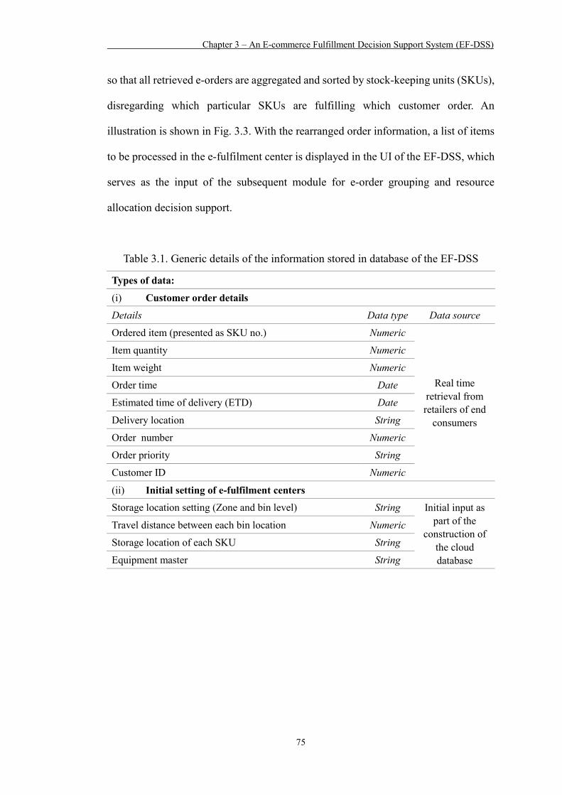
Chapter 3 – An E-commerce Fulfillment Decision Support System (EF-DSS)
75
so that all retrieved e-orders are aggregated and sorted by stock-keeping units (SKUs),
disregarding which particular SKUs are fulfilling which customer order. An
illustration is shown in Fig. 3.3. With the rearranged order information, a list of items
to be processed in the e-fulfilment center is displayed in the UI of the EF-DSS, which
serves as the input of the subsequent module for e-order grouping and resource
allocation decision support.
Table 3.1. Generic details of the information stored in database of the EF-DSS
Types of data:
(i) Customer order details
Details Data type Data source
Ordered item (presented as SKU no.) Numeric
Real time retrieval from retailers of end
consumers
Item quantity Numeric
Item weight Numeric
Order time Date
Estimated time of delivery (ETD) Date
Delivery location String
Order number Numeric
Order priority String
Customer ID Numeric
(ii) Initial setting of e-fulfilment centers Storage location setting (Zone and bin level) String Initial input as
part of the construction of
the cloud database
Travel distance between each bin location Numeric
Storage location of each SKU String
Equipment master String

Chapter 3 – An E-commerce Fulfillment Decision Support System (EF-DSS)
76
Fig. 3.3. Consolidation and sorting of customer e-order in EF-DSS
3.5 E-order grouping module (EGM)
This module groups SKUs into several batches so that logistics practitioners can
perform batch order picking accordingly. Information stored and processed in the
previous module, including the sorted order details and storage location of SKUs
pending to be picked, serves as the inputs of this module. The grouping of e-orders is
done by a GA mechanism, which starts with encoding the proposed order grouping
model into a chromosome. An initial population of the e-orders grouping solution is
then formed, followed by the fitness of each chromosome being evaluated with the
adoption of a quantitative model that includes constraints as the representation of the
order grouping criteria. Prior to reaching the termination criteria, crossover and
mutation operations are repeatedly performed to generate different sets of solutions.
Upon fulfilling the termination criteria, the chromosome with smallest fitness value is
selected as the near-optimal solution, which is then decoded and transformed into a
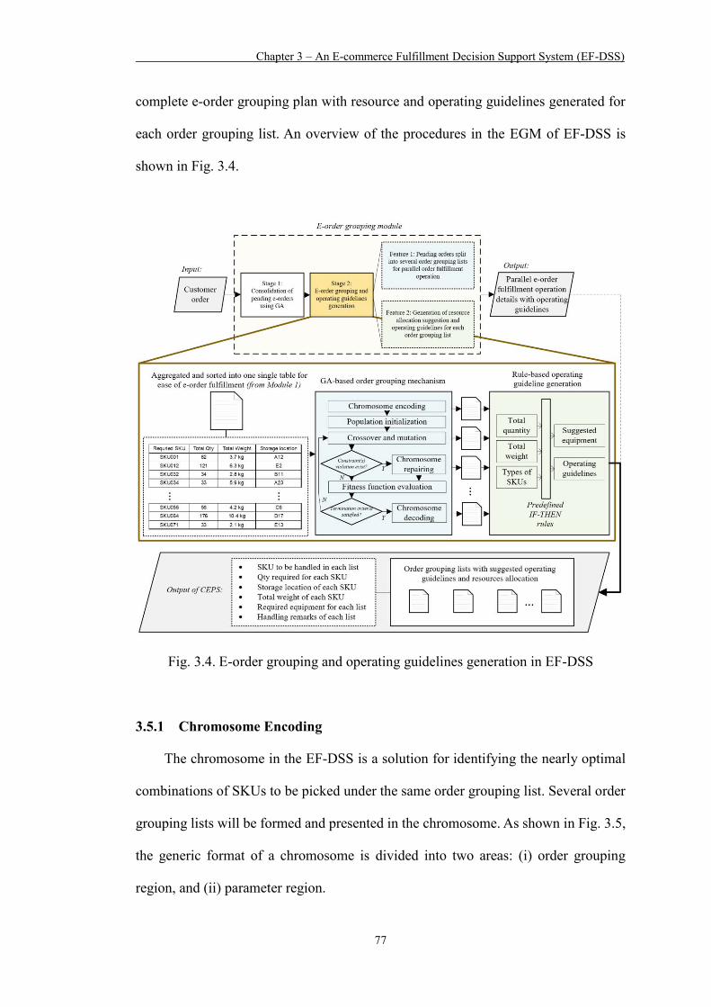
Chapter 3 – An E-commerce Fulfillment Decision Support System (EF-DSS)
77
complete e-order grouping plan with resource and operating guidelines generated for
each order grouping list. An overview of the procedures in the EGM of EF-DSS is
shown in Fig. 3.4.
Fig. 3.4. E-order grouping and operating guidelines generation in EF-DSS
3.5.1 Chromosome Encoding
The chromosome in the EF-DSS is a solution for identifying the nearly optimal
combinations of SKUs to be picked under the same order grouping list. Several order
grouping lists will be formed and presented in the chromosome. As shown in Fig. 3.5,
the generic format of a chromosome is divided into two areas: (i) order grouping
region, and (ii) parameter region.

Chapter 3 – An E-commerce Fulfillment Decision Support System (EF-DSS)
78
(i) Order grouping region
The basic idea of the chromosome encoding scheme of this region comes from
Lin et al. (2014). The value of each gene is a real number, where “0” represents the
depot, and other values indicate the storage bin location. Take the chromosome in Fig.
6 as an example, a chromosome “112 114 145 0 243 231 212 321 0 410 412 413 415
0” can be interpreted as 0-112-114-145-0, 0-243-231-212-321-0, and 0-410-412-413-
415-0, which implies that a total of three order grouping lists are generated, with the
storage location under each order grouping list specified in the chromosome. For
example, the order grouping list with chromosome “0-112-114-145-0” denotes that
three storage bin locations, i.e. 112, 114 and 145, are to be travelled to when the
operator in the e-fulfilment center follows this order grouping list to execute e-order
fulfilment operations.
(ii) Parameter region
The parameter region shows the chromosome genes which can further be
classified into three different areas: total weight, total quantity and required equipment.
Based on the order grouping solutions generated in the chromosome genes in the order
grouping region, the corresponding total weight (W), total quantity (Q) and types of
SKUs involved (S) of each order grouping list are displayed. The value of total weight
(W), total quantity (Q) and the type of SKUs involved in the order grouping list, are
used to generate pre-set operating guidelines and suggest the required equipment
based on the pre-defined rules in the rule-based inference system. As shown in Fig. 6,
the corresponding total weight, total quantity and required equipment of order
grouping list 1, i.e. chromosome gene B1j, where j = 1, 2, …, N, is denoted as W1, Q1,
S1 respectively. The length of the chromosome in the parameter region depends on the
number of order picking lists generated for the current problem.

Chapter 3 – An E-commerce Fulfillment Decision Support System (EF-DSS)
79
Fig. 3.5. The generic format of a chromosome
3.5.2 Population Initialization
An initial population of the feasible solution represented as a chromosome is
formed. Assuming that the initial population size is s and the parameter index p is set
as 1. For p < s, then p = p + 1, so as to continue generating chromosomes, else stop.
Due to a large number of storage locations required to be visited in an e-fulfilment
center for order picking of various items ordered by different online customers, the
long length of a chromosome suggests that a large population size is required for
generating a considerable number of possible combinations in crossover and mutation
operations in the GA mechanism.
3.5.3 Fitness Evaluation
A fitness function that minimizes the one-dimensional travel distance between
two adjacent nodes, i.e. storage bin location, is used to evaluate the fitness of each
chromosome. Considering the placement and alignment of a series of pallet racks in
parallel as a common facility layout in the storage area of e-fulfilment centers,
warehouses and distribution centers, a distance matrix that calculates and indicates the
inter-bin distances among each storage bin is proposed, instead of a conventional
computation of the distance between two adjacent nodes i and i+1 with coordinates
(xi, yi) and (xj, yj) using Di,j = √(𝑥𝑗 − 𝑥𝑖)2 + (𝑦𝑗 − 𝑦𝑖)2. The preparation of an inter-bin

Chapter 3 – An E-commerce Fulfillment Decision Support System (EF-DSS)
80
distance matrix is considered to be a more rational and appropriate one, in comparison
to a simple calculation of the distance between two adjacent nodes using their x and y
coordinates, due to the fact an operator who is about to visit two storage bin locations,
say bin A1 and bin B1 in Fig. 3.6, must be either picking route 1 or route 2, as
illustrated in Fig. 3.6. A distance matrix that illustrates the shortest possible travel
distance between each bin therefore achieves a better accuracy for fitness function
evaluation. The shortest inter-bin travel distance (Di,j) for bin i and j is calculated by
Eq. 11:
Di,j = min [Xi + Xj, (L - Xi) + (L – Xj)] + Ns × S + NA × A (11)
where Xi is distance between x-coordinate of storage bin i and the starting position of
the aisle (the origin), L is the total length of an aisle, NA and Ns are respectively the
number of aisles and storage bins vertically travelled across, and A and S are
respectively the widths of an aisle and storage bin.
Fig. 3.6. An example of the shortest inter-bin travel distance calculation between two
storage bins

Chapter 3 – An E-commerce Fulfillment Decision Support System (EF-DSS)
81
For each order grouping problem, n out of N storage bins are required to be
visited to pick up the items ordered by online customers, where N is the total number
of storage bins, and n ≤ N. With the N×N distance matrix that contains all inter-bin
shortest travel distances in the e-fulfilment center, the inter-bin distances among n out
of N storage bins are required to be extracted from the parent distance matrix, by
filtering out the inter-bin distances of all storage bins which will not be visited in this
order fulfilment wave. This allows the GA mechanism to evaluate the fitness of each
chromosome by only coping with the inter-bin distances of the n storage bins
concerned in the current problem using the n×n distance matrix extracted from the
original N×N distance matrix. The quantitative format of EF-DSS for e-order grouping
is presented below. The notations are depicted in Table 3.2. Eq. (12) determines the
shortest travel distance of all generated chromosomes. Constraint (3) ensures that the
order grouping list includes visiting storage bin location j immediately after storage
bin location i. Constraints (14) and (15) ensure that each travel path only has one order
grouping list and each storage bin location is included in only one single order
grouping list. Constraints (16) and (17) respectively specify the volume and weight
limit of an order grouping list. Constraint (18) ensures the continuity of path.
𝑀𝑖𝑛𝑖𝑚𝑖𝑧𝑒 ∑ ∑ ∑ 𝐷𝑖𝑗𝑥𝑖𝑗𝑔
𝐺
𝑔=1
𝑁
𝑗=1
(12)
𝑁
𝑖=1
𝑥𝑖𝑗𝑔 = { 1, if order grouping list g includes visiting bin location j just after i
0, otherwise
∀g ∈ 𝐺 (13)
∑ ∑ 𝑥𝑖𝑗𝑔
𝑔∈𝐺
= 1, ∀ 𝑗 ∈ 𝑁 (14)
𝑖∈𝑁
∑ ∑ 𝑥𝑖𝑗𝑔
𝑔∈𝐺
= 1, ∀ 𝑖 ∈ 𝑁 (15)
𝑗∈𝑁

Chapter 3 – An E-commerce Fulfillment Decision Support System (EF-DSS)
82
∑ ∑ 𝑣𝑖𝑥𝑖𝑗𝑔
𝑗∈𝑁
≤ 𝑉𝑔, ∀ 𝑔 ∈ 𝐺 (16)
𝑖∈𝑁
∑ ∑ 𝑤𝑖𝑥𝑖𝑗𝑔
𝑗∈𝑁
≤ 𝑊𝑔, ∀ 𝑔 ∈ 𝐺 (17)
𝑖∈𝑁
∑ 𝑥𝑖𝑗𝑔 = ∑ 𝑥𝑗𝑖𝑔
𝑗∈𝑁𝑗≠𝑖
, ∀ 𝑖 ∈ 𝑁𝑗∈𝑁𝑗≠𝑖
, ∀ 𝑔 ∈ 𝐺 (18)
Table 3.2. Notation table for quantitative model of EF-DSS
Notation Definition G Index set of all order grouping lists, G={1,2,…,g} N Index set of all storage bin location, N={1,2,…,n} g Index for order grouping list i, j Index for storage bin location 𝒗𝒊 Volume of items to be picked at storage bin location i 𝒘𝒊 Weight of items to be picked at storage bin location i 𝑽𝒈 Volume limit of order grouping list g 𝑾𝒈 Weight limit of order grouping list g 𝑫𝒊𝒋 Shortest inter-bin distance between storage bin location i and j 𝒙𝒊𝒋𝒈 Binary variable indicating whether order grouping list g ∈ G travels
storage bin location i and j
3.5.4 Genetic Operations
The genetic operations in GA for generating new offspring involve chromosome
crossover and mutation operations. Appropriate chromosomes are selected prior to
performing the genetic operations. Among the common selection operators of
chromosomes, the tournament selection operator is proposed over the roulette-wheel-
based proportionate selection operator, as the latter approach is unable to handle
minimization problems directly. The former approach can handle both maximization
and minimization problems and the complete selection process can be performed
quickly. Upon selection of the chromosomes, they are transferred from the parent pool
to the mating pool for creating new offspring through combining the selected

Chapter 3 – An E-commerce Fulfillment Decision Support System (EF-DSS)
83
chromosomes in crossover operations and changing the genes in the chromosomes in
mutation operations, with a crossover rate and mutation rate pre-defined. In crossover
operations, a crossover probability index between 0 and 1 is randomly generated for
each chromosome in the mating pool, so that chromosomes with a crossover
probability index less than the pre-defined rate of crossover are chosen for performing
crossover operations. In mutation operations, a random number between 0 and 1 is
generated for each gene in the chromosome. Genes with a random number less than
the rate of mutation undergo mutation operations. After crossover and mutation of
chromosomes, chromosome repairing is performed to fix the chromosomes to ensure
every chromosome obeys the encoding scheme. Violations of the encoding scheme
include the inconsistencies between two regions of the chromosome and violations of
the volume or weight constraints of an order grouping list. The repairing operation,
which can be classified into three stages (Ho et al., 2008), i.e. forward repairing,
backward repairing and limit repairing, is performed.
3.5.5 Termination criteria and chromosome decoding
The fitness of each chromosome is again evaluated for identifying the best order
grouping solution, namely a chromosome with the smallest fitness value. The
maximum number of iterations is chosen as the pre-defined termination criteria of the
GA mechanism in EF-DSS. When the number of iterations has reached this threshold
value, the GA iteration process is stopped. The best chromosome is then selected as
the near-optimal solution and decoded into a readable format of order grouping
solutions, allowing users to obtain the suggested number of order grouping lists
required and the details of each order grouping list, including the storage bin locations
sequence to be visited in each order grouping list and the corresponding items with
quantity information to be handled at each storage bin location.

Chapter 3 – An E-commerce Fulfillment Decision Support System (EF-DSS)
84
3.5.6 Rule-based guidelines decision support
Rule-based operating guidelines decision support is generated in addition to the
order grouping solutions. As the operating procedures and equipment selections vary
depending on the nature of an order, the total weight and quantity of each order
grouping list as indicated in the parameter region of the chromosome, along with the
product categories handled in each order grouping list, serve as the antecedents, i.e.
the “IF” part of the “IF-THEN” rules pre-defined in EF-DSS. The required equipment
and a set of suggested operating procedures are the consequent, the “THEN” part of a
rule. Among the two broad kinds of inference engines used in rule-based systems,
forward chaining and backward chaining systems, the former one, that is, a data-
driving reasoning strategy, is adopted in EF-DSS so as to process the known
parameters given in the parameter region of the chromosome to keep using the “IF-
THEN” rules to suggest an appropriate set of operating procedures and handling
equipment.
With the order grouping decision support and knowledge support through
suggesting an appropriate set of operating procedures and equipment, the e-commerce
order processing flow in the e-fulfilment center is reengineered, as the top
management of the e-fulfilment center can flexibly consolidate pending a large
number of discrete, small lot-sized online customer orders and then release the jobs in
waves with clear instructions of how these jobs are to be handled.
3.6 E-order batch releasing module (EBRM)
To deploy the warehouse postponement strategy in e-fulfilment distribution
centres, not only do the logistics service providers need to consolidate the incoming
e-orders and group them into different batches for the subsequent bulk order
processing, but determining an appropriate timing to stop the e-order consolidation
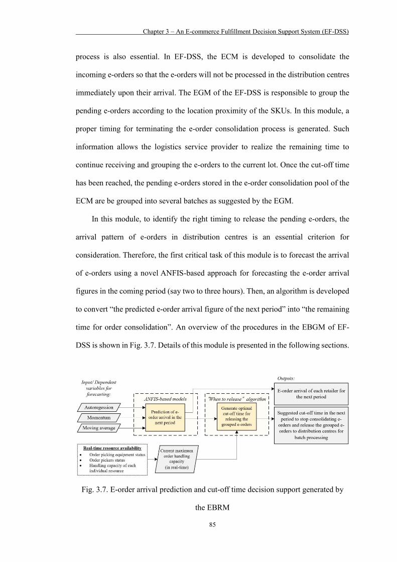
Chapter 3 – An E-commerce Fulfillment Decision Support System (EF-DSS)
85
process is also essential. In EF-DSS, the ECM is developed to consolidate the
incoming e-orders so that the e-orders will not be processed in the distribution centres
immediately upon their arrival. The EGM of the EF-DSS is responsible to group the
pending e-orders according to the location proximity of the SKUs. In this module, a
proper timing for terminating the e-order consolidation process is generated. Such
information allows the logistics service provider to realize the remaining time to
continue receiving and grouping the e-orders to the current lot. Once the cut-off time
has been reached, the pending e-orders stored in the e-order consolidation pool of the
ECM are be grouped into several batches as suggested by the EGM.
In this module, to identify the right timing to release the pending e-orders, the
arrival pattern of e-orders in distribution centres is an essential criterion for
consideration. Therefore, the first critical task of this module is to forecast the arrival
of e-orders using a novel ANFIS-based approach for forecasting the e-order arrival
figures in the coming period (say two to three hours). Then, an algorithm is developed
to convert “the predicted e-order arrival figure of the next period” into “the remaining
time for order consolidation”. An overview of the procedures in the EBGM of EF-
DSS is shown in Fig. 3.7. Details of this module is presented in the following sections.
Fig. 3.7. E-order arrival prediction and cut-off time decision support generated by
the EBRM
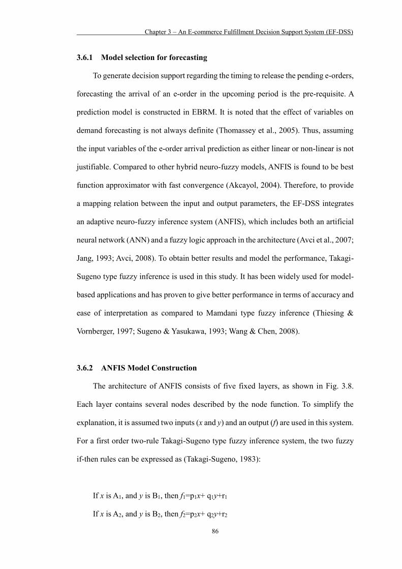
Chapter 3 – An E-commerce Fulfillment Decision Support System (EF-DSS)
86
3.6.1 Model selection for forecasting
To generate decision support regarding the timing to release the pending e-orders,
forecasting the arrival of an e-order in the upcoming period is the pre-requisite. A
prediction model is constructed in EBRM. It is noted that the effect of variables on
demand forecasting is not always definite (Thomassey et al., 2005). Thus, assuming
the input variables of the e-order arrival prediction as either linear or non-linear is not
justifiable. Compared to other hybrid neuro-fuzzy models, ANFIS is found to be best
function approximator with fast convergence (Akcayol, 2004). Therefore, to provide
a mapping relation between the input and output parameters, the EF-DSS integrates
an adaptive neuro-fuzzy inference system (ANFIS), which includes both an artificial
neural network (ANN) and a fuzzy logic approach in the architecture (Avci et al., 2007;
Jang, 1993; Avci, 2008). To obtain better results and model the performance, Takagi-
Sugeno type fuzzy inference is used in this study. It has been widely used for model-
based applications and has proven to give better performance in terms of accuracy and
ease of interpretation as compared to Mamdani type fuzzy inference (Thiesing &
Vornberger, 1997; Sugeno & Yasukawa, 1993; Wang & Chen, 2008).
3.6.2 ANFIS Model Construction
The architecture of ANFIS consists of five fixed layers, as shown in Fig. 3.8.
Each layer contains several nodes described by the node function. To simplify the
explanation, it is assumed two inputs (x and y) and an output (f) are used in this system.
For a first order two-rule Takagi-Sugeno type fuzzy inference system, the two fuzzy
if-then rules can be expressed as (Takagi-Sugeno, 1983):
If x is A1, and y is B1, then f1=p1x+ q1y+r1
If x is A2, and y is B2, then f2=p2x+ q2y+r2
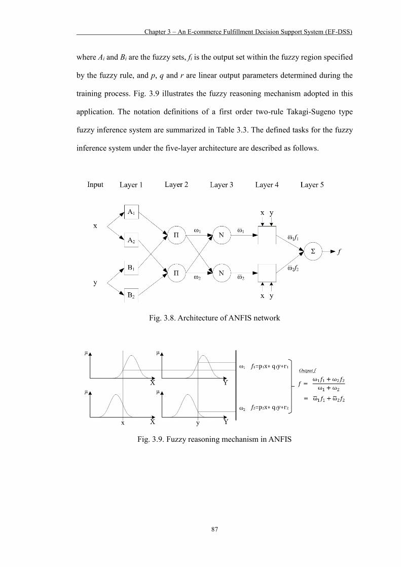
Chapter 3 – An E-commerce Fulfillment Decision Support System (EF-DSS)
87
where Ai and Bi are the fuzzy sets, fi is the output set within the fuzzy region specified
by the fuzzy rule, and p, q and r are linear output parameters determined during the
training process. Fig. 3.9 illustrates the fuzzy reasoning mechanism adopted in this
application. The notation definitions of a first order two-rule Takagi-Sugeno type
fuzzy inference system are summarized in Table 3.3. The defined tasks for the fuzzy
inference system under the five-layer architecture are described as follows.
Fig. 3.8. Architecture of ANFIS network
Fig. 3.9. Fuzzy reasoning mechanism in ANFIS

Chapter 3 – An E-commerce Fulfillment Decision Support System (EF-DSS)
88
Table 3.3. Notation definitions for ANFIS network architecture
Network architecture of a typical first order two-rule Takagi-Sugeno type fuzzy
inference system (refer to Figs. 3.8 and 3.9):
Notation Definition
x , y Inputs
f Overall output
Ai, Bi Fuzzy sets
fi Output set within the fuzzy region specified by the fuzzy rule
p, q, r Linear output parameters (determined during the training process)
Oj,i Output of the ith node in layer j
µAi(x) Bell shape membership function with a parameter set of {ai, bi, ci}
ωi Firing strength of each rule
(i.e. the output of layer 2, symbolized by a Π notation)
�̅�𝒊 Ratio of the ith node firing strength to the sum of the firing strength of
all rules
(i.e. the output of layer 3, symbolized by a N notation)
Layer 1. Each node i in this layer is a square node with a node function represented
as:
O1, i = µAi(x) = 1
1+(𝑥−𝑐𝑖
𝑎𝑖)2𝑏𝑖
for i = 1, 2 (19)
where O1,i represents the output of the ith node in this layer, x is an input to node i, Ai
is the linguistic label for the input, such as short and long, and µAi(x) is the membership
function which is commonly of bell shape with a minimum and maximum value of 0
and 1 respectively. The bell shape membership function has a parameter set of {ai, bi,
ci} that is referred to as the premise parameters. These parameters change the bell
shape of the membership function automatically.

Chapter 3 – An E-commerce Fulfillment Decision Support System (EF-DSS)
89
Layer 2. Each fixed node in this layer is a circle node symbolized by a Π notation.
The output of this layer, ωi, denotes the firing strength of each rule, which is calculated
by the multiplication of the input signals:
O2, i = ωi = µAi(x) µBi(y) for i = 1, 2 (20)
Layer 3. Each fixed node in this layer is a circle node symbolized by a N notation.
The output of this layer, ω̅i, denotes the ratio of the ith node firing strength to the sum
of the firing strength of all rules, which is expressed as:
O3, i = ω̅𝑖 = ω𝑖
∑ ω𝑖=
ω𝑖
ω1+ω2 for i = 1, 2 (21)
Layer 4. Each adaptive node in this layer is a square node for calculating the
contribution of the ith node towards the overall output, which is expressed as:
O4, i = ω̅𝑖fi = ω̅𝑖(𝑝𝑖𝑥 + 𝑞𝑖𝑦 + 𝑟𝑖) for i = 1, 2 (22)
since fi represents the fuzzy if-then rules with {pi, qi, ri} being the parameter set, where
these parameters are referred to as the consequent parameters.
Layer 5. The single fixed node in this layer is a circle node symbolized by a Ʃ
notation. It computes the overall output of the network by calculating the summation
of the contribution of all rules:
O5, i = ∑ ω̅𝑖𝑓𝑖 = ∑ ω𝑖𝑓𝑖
∑ ω𝑖 = f = overall output for i = 1, 2 (23)
With the values of the premise parameters being constant, the overall output can be
expressed as the linear combination of the consequent parameters:

Chapter 3 – An E-commerce Fulfillment Decision Support System (EF-DSS)
90
f = ω1
ω1+ω2𝑓1 +
ω2
ω1+ω2𝑓2
= ω̅1𝑓1 + ω̅2𝑓2
= ω̅1(𝑝1𝑥 + 𝑞1y + 𝑟1) + ω̅2(𝑝2x + 𝑞2y + 𝑟2)
= (ω̅1𝑥)𝑝1 + (ω̅1𝑦)𝑞1+(ω̅1)𝑟1 + (ω̅2𝑥)𝑝2 + (ω̅2𝑦)𝑞2+(ω̅2)𝑟2 (24)
In order to allow the fuzzy inference system to learn through the training data
sets, the hybrid learning algorithm for ANFIS is used. The algorithm combines the
back-propagation gradient descent and least square methods to create a fuzzy inference
system with the membership functions being adjusted iteratively through updating the
parameters. To update the parameters, for instance, the algorithm is composed of a
forward pass and a backward pass. The forward pass makes use of least square
methods to optimize the consequent parameters, i.e. pi, qi, ri. with the premise
parameters, i.e. ai, bi, ci, fixed as constant. Immediately after obtaining the optimal
values of the consequent parameters, the backward pass starts by making use of the
gradient descent method to update the optimal values of the premise parameters.
Chapter 5 illustrates the application of ANFIS in the perspective of e-commerce order
management in two distribution centres.
The output of the ANFIS model is the predicted e-order arrival within a specified
period of time. Such e-order arrival prediction allows logistics practitioners to
determine the cut-off time of the pending e-orders so that an appropriate size of e-
orders in terms of the weight of the orders (measured in kg), can be grouped and
subsequently released in a batch for bulk order picking in the distribution centres or
order fulfilment centres. The real-time availability of resources, such as order picking
equipment and order pickers, is also taken into consideration, so as to ensure that there

Chapter 3 – An E-commerce Fulfillment Decision Support System (EF-DSS)
91
are sufficient resources to handle the size of the grouped e-orders. Details of the
decision support for determining the cut-off time are further discussed in section 3.6.3.
In the structural design of the ANFIS model for forecasting the e-order arrival in
distribution centres, the model construction process includes three sequential stages,
as depicted in Fig. 3.2, they are: Stage I – Design Considerations Fitness Evaluation,
Stage II – Model Training and Testing, and Stage III – Performance Evaluations.
Details steps for model construction under each stage are discussed in the following
sections.
3.6.2.1 Stage I – Design Considerations
In Stage I – Design Considerations, the initial model settings are determined and
configured based on the operating size and nature of business of the logistics service
providers. There are in total 5 steps involved in this stage:
Step 1 – Determine the cycle time for reviewing the e-order consolidation cut-off
policy,
Step 2 – Identify the input and output variables in the ANFIS models,
Step 3 – Select and extract dataset for model training and testing,
Step 4 – Define the universe of disclosure for each input parameter, and
Step 5 – Define the type of output functions for each output parameter.
Step 1 – Determine the cycle time for reviewing the e-order consolidation cut-off
policy
The e-order consolidation cut-off time is the final output of the EBRM. It denotes
how much time is left for the logistics service providers to continue consolidating the
e-orders before releasing them in batch. To generate such decision support, users are
required to use the EBRM of the EF-DSS periodically to forecast the number of e-

Chapter 3 – An E-commerce Fulfillment Decision Support System (EF-DSS)
92
orders that will be arriving at the distribution centres in the coming “period”. However,
it is up to the decision makers to decide how long should the “period” be. Therefore,
prior to the construction of the ANFIS-based forecasting models, the “period”, that is,
the cycle time for reviewing the e-order consolidation cut-off time is required to be
determined. By identifying the cycle time, the ANFIS-based forecasting model in the
ERBM is suggested to be used at the end of each cycle. For example, if the cycle time
is 2 hours, then the operators can use the ERBM of the EF-DSS to obtain the predicted
number of e-orders in the coming two hours using the ANFIS forecasting model.
Consequently, by using the proposed algorithm presented in section 3.6.3, the current
available order handling capacity is compared with the predicted number of e-orders
in the coming two hours, so as to determine how much time is left for batch release of
the pending e-orders.
There are two factors for determining the cycle time for reviewing the e-order
consolidation cut-off time: the maximum order handling capacity in the e-fulfilment
distribution centres and the average number of orders (in kg) received per hour. The
maximum order handling capacity is an estimation of the maximum weight of orders
(in kg) that can be handled by the available resources, assuming all resources including
the order picking equipment and order pickers are completely idle and can be fully
allocated for handling the e-orders once they are released in batch for bulk processing
in the distribution centres. For the average number of orders received per hour, the
figure is collected based on the historical order receiving amount. To better illustrate
how the cycle time is identified, an example is given in Table 3.4. If the maximum
order handling capacity of a distribution centre is 200 kg, and the statistics reveals that
the average number of e-orders received per hour is only 60 kg. In this regard, the
approximate cut-off time for consolidating the e-commerce orders is 3.33 hours (by
dividing the order handling capacity by the number of e-orders received per hour).

Chapter 3 – An E-commerce Fulfillment Decision Support System (EF-DSS)
93
Therefore, the cycle time for making a periodic review of the cut-off time must be less
than 3.33 hours, say 2 or 3 hours, to avoid any overloading of resources due to
consolidating too many e-orders at a single time. With the cycle time (“period”)
identified, the output of the ANFIS forecasting models to be built in the EBRM of the
EF-DSS would be the e-order arrival figure in the coming period.
Table 3.4. Example of cycle time determination
Considerations in determining the cycle time for
reviewing the e-order consolidation cut-off time Example
Maximum order handling capacity in distribution centres 200 kg
Historical average number of orders received per hour 60 kg
Approximate cut-off time for e-order consolidation: Every 3.33 hours
(= 200/60)
Cycle time for periodic review: Every 2 or 3 hours
Step 2 – Identify the input and output variables in the ANFIS models
After determining the cycle time (“period”) for reviewing the cut-off policy, the
output variable of the ANFIS models is identified, that is, Qd(t+1), the predicted arrival
of the e-orders (in kg) in the upcoming period t+1 in the current day d. For the input
variables, it is noted that the prediction subject, Qd(t+1), is time-series data. In this
regard, three types of variables are considered as the determinants of the time-series-
type e-order arrival figure: actual e-order arrival of the previous n1 periods, volatility
of e-order arrival among the previous n2 periods, and the n3-period simple moving
average. The justification of selecting these input variables is presented in Table 3.5.

Chapter 3 – An E-commerce Fulfillment Decision Support System (EF-DSS)
94
Table 3.5. Justifications of the input variables of the ANFIS forecasting models
Input variable Justifications
Actual e-order arrival of
the previous n1 periods
In time-series data prediction study, lag variables, i.e.
previous figures, are the essential indicators for
predicting the next figure. Thus, the actual e-order
arrival in the previous n1 periods, i.e. period t, t-1, t-
2, …, t-n1, are considered as essential prediction
indicators for predicting the e-order arrival figure at
the upcoming period t+1.
Volatility of e-order arrival
among the previous n2
periods
The volatility of previous e-order arrival
(momentum) is an essential indicator of the trend of
the time-series-based e-order arrival. This indicator
has been used to predict the stock prices. Tanaka-
Yamawaki & Tokuoka (2007) introduced one and
two-order momentum as a technical indicator of
intra-day stock price prediction. Chang et al. (2011)
also introduced one and two-order momentum for
forecasting the stock prices. Thus, this study
considers both one and two-order momentum of e-
order arrival as the input variables.
n3-period simple moving
average
Simple moving average is another obvious figure
that has been commonly introduced as a prediction
indicator. Therefore, a two-period and three-period
simple moving average are introduced as the input
variables for ANFIS forecasting modelling.

Chapter 3 – An E-commerce Fulfillment Decision Support System (EF-DSS)
95
Step 3 – Select and extract dataset for model training and testing
The training and testing process is a critical model construction procedure to build an
ANFIS model with satisfactory prediction capability. To effectively train and then test
the models, a real production data set needs to be gathered and extracted from the
distribution centre where e-order fulfilment operations take place. With the cut-off
review cycle identified during Step 1 – Determine the cycle time for reviewing the e-
order consolidation cut-off policy, the data sets are pre-processed and converted into
useful input values for the proposed ANFIS models. For example, if the cut-off review
cycle is 2 hours, the data set is then pre-processed to demonstrate the e-order arrival
figures of every 2 hours. An example of data set in 2-hour time interval is shown in
Table 3.6.
Table 3.6. An example of data set in 2-hour time interval
Time
Date 0-2 2-4 4-6 6-8 8-10 10-12 12-14 14-16 16-18 18-20 20-22 22-24
Mon 14 21 12 14 25 46 49 55 68 53 79 94 Tue 41 32 25 10 27 47 56 78 84 63 89 84 Wed 45 34 21 22 35 42 39 52 73 81 71 78 Thu 43 32 30 19 21 41 46 52 62 73 75 68 Fri 56 42 21 21 37 47 52 62 57 69 73 68 Sat 78 52 31 23 36 68 58 63 67 73 83 84 Sun 94 77 47 23 49 64 72 62 89 52 96 67
Step 4 – Define the universe of disclosure for each input parameter
To achieve the best result generated from the ANFIS model, system parameter
modifications are critical. In the MATLAB’s ANFIS editor, different types of
membership functions (MFs), such as triangular (Tri), trapezoidal (Trap), generalized
bell (Gbell), Gaussian curve (Guass), Gaussian combination, Π-shaped, difference

Chapter 3 – An E-commerce Fulfillment Decision Support System (EF-DSS)
96
between two sigmoid functions, and product of two sigmoid functions, are available
for selection. In addition, the number of MFs for each input and the types of output
MFs (either constant or linear) can also be modified. Due to a large number of possible
combinations of the parameter settings of the ANFIS model, the best combination of
the ANFIS model needs to be identified. A summary of the configurable model settings
that need to be tested is presented in Table 3.7.
Table 3.7. A summary of the configurable model settings that need to be tested
Types of model configuration Configurations to be tested
Initial FIS generation Grid partitioning
Types of input MFs* Tri/Trap/Gbell/Guass
Number of MFs for each input* 2/3/4
Types of output function* Constant /linear
Learning algorithm Least square method and
Back-propagation gradient descent
method
*Further experiments were made to identify the best MFs characteristics
Step 5 – Define the type of output functions for each output parameter
Apart from a number of configurable settings available that are required for
proper selection through performing model testing, the output function of the ANFIS
model can either be “Constant” or “Linear”. Therefore, during Stage II – Model
Training and Testing, different combinations of configurable settings need to be tested
so as to identify the best combination of setting for an ANFIS model.

Chapter 3 – An E-commerce Fulfillment Decision Support System (EF-DSS)
97
3.6.2.2 Stage II – Model Training and Testing
The dataset, which is selected in Step 3 - Select and extract dataset for model
training and testing under Stage I, needs to be split into two different data sets, i.e.
training dataset and testing dataset. Usually, the training data set contains 70% or 90%
of all data and the remaining data serves as the testing data set (Sánchez et al., 2007).
The training data set is used to train and build the adaptive network. The testing data
set is used to determine if any over fitting of model occurs during training. Therefore,
in order to check the generalization capability of the developed neural system and to
avoid the model from overfitting the training data set, the trained fuzzy inference
system under different combinations of settings is then applied using the testing data
set. The optimal model setting for an ANFS model can then be identified.
3.6.2.3 Stage III – Performance Evaluations
With the best setting obtained for the developed ANFIS models, they are then
compared with an autoregressive integrated moving average (ARIMA) model for
further performance validation. The root-mean square error (RMSE), mean absolute
deviation (MAD) and mean absolute percentage error (MAPE), which are respectively
given by Eq. (25), (26), and (27), are adopted for model performance comparisons.
RMSE = √∑ (𝐴𝑡−𝑄𝑡)2𝑛
𝑡=1
𝑛 (25)
MAD =1
𝑛∑ |𝐴𝑡 − 𝑄𝑡|𝑛
𝑡=1 (26)
MAPE =1
𝑛∑ |
𝐴𝑡−𝑄𝑡
𝐴𝑡∗ 100|𝑛
𝑡=1 (27)

Chapter 3 – An E-commerce Fulfillment Decision Support System (EF-DSS)
98
where At and Qt are respectively the actual arrival of e-order and predict arrival of e-
order (in terms of weight in kg) at period t, and n is the number of data patterns in the
independent data set.
3.6.3 Algorithm for Determining “When to release” decision
This sub-module makes use of the output of the ANFIS model in EBRM of the
EF-DSS, i.e. the predicted arrival of e-commerce orders in the upcoming period
measured by the weight in kg, to generate decision support for logistics practitioners
so as to adjust the cut-off frequency of releasing the grouped orders for actual order
picking operations in a batch. To compute the cut-off time of the e-order grouping, the
proposed approach in the EF-DSS suggests taking the maximum order handling
capacity in the distribution centre into consideration. The maximum order handling
capacity, Qmax, can be obtained by identifying the total weight that can be handled by
the resources for order handling, such as equipment and order pickers, which are
currently idle and available for performing picking operations of e-orders. With the
known constant value of Qmax, EF-DSS is able to automatically generate the cut-off
time, denoted as Tfinal, with the notation definitions shown in Table 3.8 and the
underlying calculations as described below.
In order to avoid any potential over-utilization of the order handling resources,
especially human resources, the maximum allowable order handling capacity (Qmax)
is multiplied by a constant factor k (in %), to give an adjusted order handling capacity
(Qadjusted). It is recommended that the value of k should be within the range of 0.6 to
0.8, based on the suggestion given by domain experts. To obtain the current remaining
order handling capacity (Qremaining), the adjusted order handling capacity is subtracted
by the total weight of pending orders in the e-order consolidate pool (Qcurrent), which
is expressed as:

Chapter 3 – An E-commerce Fulfillment Decision Support System (EF-DSS)
99
𝑄𝑎𝑑𝑗𝑢𝑠𝑡𝑒𝑑 = 𝑄𝑚𝑎𝑥 × 𝑘 (28)
𝑄𝑟𝑒𝑚𝑎𝑖𝑛𝑖𝑛𝑔 = 𝑄𝑎𝑑𝑗𝑢𝑠𝑡𝑒𝑑 − 𝑄𝑐𝑢𝑟𝑟𝑒𝑛𝑡 (29)
The predicted e-order arrival rate per minute (Qt) is computed by dividing the
predicted weight of the incoming e-orders in the upcoming period t+1 (Qd(t+1), the
output of the ANFIS model), by the total duration in the specified period (in minutes)
(n). It is expressed as:
𝑄𝑡 =𝑄𝑑(𝑡+1)
𝑛 (30)
The optimal cut-off time for batch order release can then be computed by dividing Eq.
(8) by Eq. (9), that is:
𝑇𝑜𝑝𝑡𝑖𝑚𝑎𝑙 =𝑄𝑟𝑒𝑚𝑎𝑖𝑛𝑖𝑛𝑔
𝑄𝑡 (31)
In order to avoid any e-order pending in the e-order consolidation pool for too long a
duration, an additional variable, Tmax, is introduced. It is defined as the maximum
allowable waiting time of an e-order pending in the e-order consolidation pool. The
purpose of introducing this variable is to govern the final suggested output of the
EAPS, i.e. the cut-off time of e-orders (Tfinal), so that Tfinal would not exceed the
maximum allowable waiting time of the e-order pending in the e-order consolidation
pool. The logic is mathematically expressed as:
𝑇𝑓𝑖𝑛𝑎𝑙 = {T𝑜𝑝𝑡𝑖𝑚𝑎𝑙 for T𝑜𝑝𝑡𝑖𝑚𝑎𝑙 ≤ 𝑇𝑚𝑎𝑥
T𝑚𝑎𝑥 for T𝑜𝑝𝑡𝑖𝑚𝑎𝑙 > 𝑇𝑚𝑎𝑥 (32)

Chapter 3 – An E-commerce Fulfillment Decision Support System (EF-DSS)
100
Table 3.8. Notation definitions for the cut-off frequency decision support in EBRM
Cut-off frequency decision support model:
Notation Definition Unit of measurement
Qmax Maximum allowable order handling capacity kg Qcurrent Total weight of pending orders in the e-order
consolidation pool kg
Qd(t+1) Predicted weight of incoming orders of the upcoming period t+1 (Output of the ANFIS model)
kg per period
Qt Predicted e-order arrival rate per minute kg per minute n Total minutes in the specified period - k Constant factor for creating buffer for order handling % Toptimal Optimal cut-off time for batch order release minutes Tmax Maximum allowable waiting time of an e-order
pending in the e-order consolidation pool minutes
Tfinal Suggested cut-off time remaining for batch order release (Final output of the EAPS)
minutes
The final output of the EBRM enables decision makers to realize how long the e-
order consolidation pool can still be collecting e-orders before they are released in
batch in the distribution centres for performing the subsequent batch order picking
operations. The output of this module, in conjunction with the use of EGM to group
the pending e-orders into several batches for batch order picking in the distribution
centres, allows logistics practitioners to effectively apply the concept of warehouse
postponement. The order fulfilment process is re-engineered from conventionally
handling orders on an individual basis to handling orders in a batch, as the incoming
e-orders can be consolidated in a pool and the subsequent warehouse operations can
be delayed until the last possible moment.
The sequence of generating decision support for e-order handling is to first use
the EBRM to obtain the suggested cut-off time for order batching, followed by the use
of EGM for systematically grouping the consolidated orders, which are pending in the

Chapter 3 – An E-commerce Fulfillment Decision Support System (EF-DSS)
101
consolidation pool of the ECM, into several orer batches presented as order picking
lists. Warehouse operators can make use of the generated order picking lists in each
period to assign order pickers to handle the subsequent order fulfilment operations in
distribution centres or warehouses.
3.7 Summary
This chapter introduces the proposed warehouse postponement strategy for efficient
handling e-commerce orders in e-fulfilment distribution centres and describes the
system architecture of the EF-DSS, which contains three modules: ECM – for
consolidation of incoming e-orders for later batch processing in the distribution
centres, EGM – for generating e-order grouping solution for logistics service providers
to split the consolidated e-orders into several batches based on the SKUs’ location
proximity, and EBRM – for assisting the logistics service providers to determine the
cut-off time that terminates the e-order consolidation process and release of the
pending e-orders in batch. The ultimate goal of the EF-DSS is to assist logistics
practitioners in effectively deploying the warehouse postponement strategy by
providing them with decision support regarding “How e-orders are grouped for batch
processing” and “When the e-order consolidation process should be terminated for
batch releasing”.
To demonstrate the feasibility and applicability of the EF-DSS in e-fulfilment
distribution centres, system implementation procedures have to be followed. The
roadmap and details of the system implementation is presented in Chapter 4.

Chapter 4 – Implementation Procedures of the System
102
Chapter 4 – Implementation Procedures of the System
4.1 Introduction
This chapter provides a roadmap for the design and implementation of the EF-
DSS in real practice. A systematic approach on how to develop the intelligent system
for executing the proposed warehouse postponement strategy in a e-fulfillment
distribution centre is given. The development and implementation of the EF-DSS
involves six phases, as depicted in Fig. 4.1: (i) Understanding of the e-commerce order
fulfillment operating categories, (ii) Structural Formulation of an Action Plan for
System Implementation, (iii) Structural Formulation of ECM, (iv) Structural
Formulation of EGM, (v) Structural Formulation of EBRM, and (vi) System
performance review and evaluation.
Fig. 4.1. The implementation procedures of the EF-DSS

Chapter 4 – Implementation Procedures of the System
103
4.2 Phase 1 – Understanding of the E-commerce Order Fulfillment
Operating Categories
In Phase 1, the operation size and characteristics of the e-fulfillment centre are
investigated. It is an essential stage prior to any structural development of the EF-DSS,
as identifying the major bottlenecks currently encountered by the LSP is essential for
the EF-DSS to be able to tackle the problems directly. To ensure the EF-DSS can be
fitted into the LSP’s distribution centre for production use, there are three steps in this
phase: (i) Company process investigation, (ii) Problems and improvement areas
identification, and (iii) Preparation of a pilot run of the system.
4.2.1 Investigating Company Process
Information and knowledge sharing across departments can be achieved through
the integration of IT tools. With E-commerce and IT being the interrelated components
of the structural change in distribution, integration of IT tools can be regarded as the
enabler for LSPs to be efficient in processing orders at the distribution centres and
delivering them at high frequencies. To facilitate the effective information sharing
process, the order handling procedures are studied to understand the operational flow
of e-commerce orders. An example is shown in Figs. 4.2 to 4.5, demonstrating the
operational flow from inbound receiving, internal processing in distribution centres,
to outbound delivery, which requires a comprehensive process investigation to identify
the improvements needed for enhancing the operating efficiency.

Chapter 4 – Implementation Procedures of the System
104
Fig. 4.2. An example of internal process investigation for logistics order handling (1)
Fig. 4.3. An example of internal process investigation for logistics order handling (2)

Chapter 4 – Implementation Procedures of the System
105
Fig. 4.4. An example of internal process investigation for logistics order handling (3)
Fig. 4.5. An example of internal process investigation for logistics order handling (4)

Chapter 4 – Implementation Procedures of the System
106
4.2.2 Identifying Problems and Improvement Areas
Any IT system implementation requires a comprehensive study of the user
requirements in advance. The user requirement study is a typical process an IT solution
provider performs by visiting the client, i.e. the system users, or in this case, the
logistics practitioners, to listen to the voice of the customers and their requirements
for system deployment. By investigating the company operating policies and
procedures, a system feature and function list can be compiled to address the user’s
specific system requirements. An example of a system function and feature list is
shown in Fig. 4.6. Before proceeding to system design and development, interviews
and meetings with the logistics service provider are also regularly held to identify and
prioritize the logistics service provider’s concerns on the operational bottlenecks. An
official agreement between the IT developer and user is made to specify the system
specifications and other relevant issues. With the comprehensive study of the existing
order processing flow and the underlying bottlenecks or improvement areas, an action
plan for system implementation can be formulated accordingly.
Though each system user, i.e. logistics service providers, has specific
requirements and needs towards a system solution, the EF-DSS proposed in this study
is a generic system that tackles the major operational bottlenecks faced by logistics
practitioners, that is, the operating inefficiency of handling e-commerce orders due to
ineffective and manual order consolidation processes. In the following section, the
structural formulation of each module in the EF-DSS, namely ECM, EGM and the
EBRM, is presented for the structure and theoretical rationale of the EF-DSS. For any
technical issue or difficulty in system implementation in the real production
environment of distribution centres, it is suggested to consult the IT solution provider
for further advice.
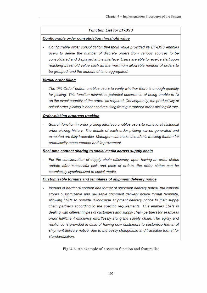
Chapter 4 – Implementation Procedures of the System
107
Fig. 4.6. An example of a system function and feature list
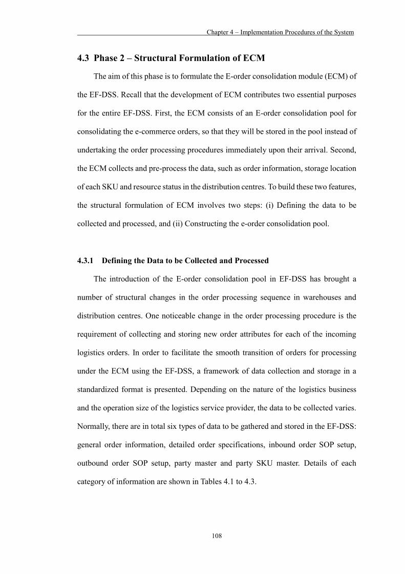
Chapter 4 – Implementation Procedures of the System
108
4.3 Phase 2 – Structural Formulation of ECM
The aim of this phase is to formulate the E-order consolidation module (ECM) of
the EF-DSS. Recall that the development of ECM contributes two essential purposes
for the entire EF-DSS. First, the ECM consists of an E-order consolidation pool for
consolidating the e-commerce orders, so that they will be stored in the pool instead of
undertaking the order processing procedures immediately upon their arrival. Second,
the ECM collects and pre-process the data, such as order information, storage location
of each SKU and resource status in the distribution centres. To build these two features,
the structural formulation of ECM involves two steps: (i) Defining the data to be
collected and processed, and (ii) Constructing the e-order consolidation pool.
4.3.1 Defining the Data to be Collected and Processed
The introduction of the E-order consolidation pool in EF-DSS has brought a
number of structural changes in the order processing sequence in warehouses and
distribution centres. One noticeable change in the order processing procedure is the
requirement of collecting and storing new order attributes for each of the incoming
logistics orders. In order to facilitate the smooth transition of orders for processing
under the ECM using the EF-DSS, a framework of data collection and storage in a
standardized format is presented. Depending on the nature of the logistics business
and the operation size of the logistics service provider, the data to be collected varies.
Normally, there are in total six types of data to be gathered and stored in the EF-DSS:
general order information, detailed order specifications, inbound order SOP setup,
outbound order SOP setup, party master and party SKU master. Details of each
category of information are shown in Tables 4.1 to 4.3.
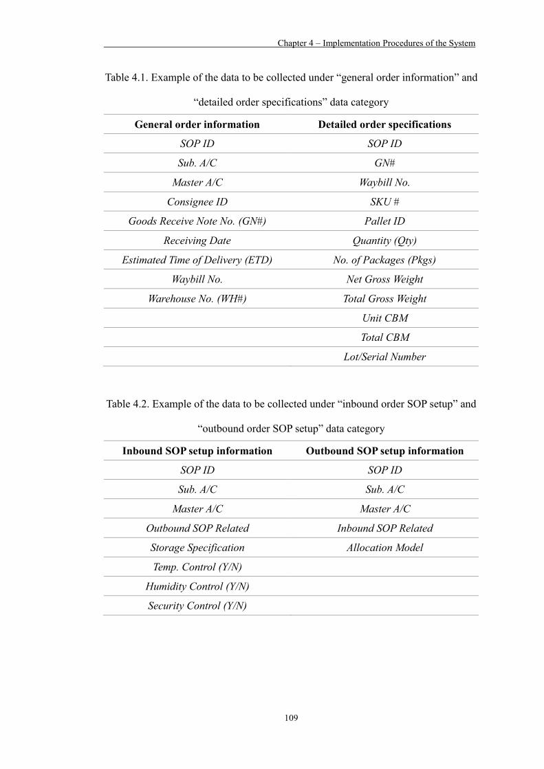
Chapter 4 – Implementation Procedures of the System
109
Table 4.1. Example of the data to be collected under “general order information” and
“detailed order specifications” data category
General order information Detailed order specifications
SOP ID SOP ID
Sub. A/C GN#
Master A/C Waybill No.
Consignee ID SKU #
Goods Receive Note No. (GN#) Pallet ID
Receiving Date Quantity (Qty)
Estimated Time of Delivery (ETD) No. of Packages (Pkgs)
Waybill No. Net Gross Weight
Warehouse No. (WH#) Total Gross Weight
Unit CBM
Total CBM
Lot/Serial Number
Table 4.2. Example of the data to be collected under “inbound order SOP setup” and
“outbound order SOP setup” data category
Inbound SOP setup information Outbound SOP setup information
SOP ID SOP ID
Sub. A/C Sub. A/C
Master A/C Master A/C
Outbound SOP Related Inbound SOP Related
Storage Specification Allocation Model
Temp. Control (Y/N)
Humidity Control (Y/N)
Security Control (Y/N)
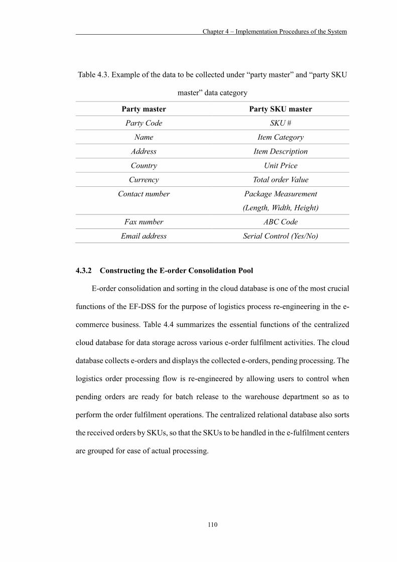
Chapter 4 – Implementation Procedures of the System
110
Table 4.3. Example of the data to be collected under “party master” and “party SKU
master” data category
Party master Party SKU master
Party Code SKU #
Name Item Category
Address Item Description
Country Unit Price
Currency Total order Value
Contact number Package Measurement
(Length, Width, Height)
Fax number ABC Code
Email address Serial Control (Yes/No)
4.3.2 Constructing the E-order Consolidation Pool
E-order consolidation and sorting in the cloud database is one of the most crucial
functions of the EF-DSS for the purpose of logistics process re-engineering in the e-
commerce business. Table 4.4 summarizes the essential functions of the centralized
cloud database for data storage across various e-order fulfilment activities. The cloud
database collects e-orders and displays the collected e-orders, pending processing. The
logistics order processing flow is re-engineered by allowing users to control when
pending orders are ready for batch release to the warehouse department so as to
perform the order fulfilment operations. The centralized relational database also sorts
the received orders by SKUs, so that the SKUs to be handled in the e-fulfilment centers
are grouped for ease of actual processing.

Chapter 4 – Implementation Procedures of the System
111
Table 4.4. Database construction for various e-logistics activities
Related
department Logistics activities Functions of the cloud database
Customer
service
department
Customer order
inquiry
Create log for track and trace of order
inquiry history
E-order collection Retrieve new orders and stores information
in the database
Documents for
order processing
Prepare required documents and import and
export, update the documentation
completion status of each order
Shipment
notification to
customers
Generate shipment notification templates
for notifying customers of their orders
ready for delivery
Warehouse
department
Order fulfilment in
e-fulfilment centers
Follow the tables for order receiving, put-
away, pick-and-pack, and delivery
operations
Order status update Update the status of e-order for order
visibility and transparency
Inventory update
Cross-checking and updating of inventory
in database and in storage areas of e-
fulfilment centers
4.4 Phase 3 – Structural Formulation of EGM
In this phase, the E-order grouping module (EGM) is constructed to split the grouped
orders into several batches for batch order picking, and the order grouping decision
support is generated through the use of a GA mechanism. Therefore, this phase
consists of two steps: (i) Building a tailor-made traveling distance matrix, and (ii)
Constructing the GA mechanism and rule-based engine.

Chapter 4 – Implementation Procedures of the System
112
4.4.1 Building a Tailor-made Traveling Distance Matrix and Sorting Algorithm
To govern the e-fulfilment operational flow, decision support for grouping SKUs
with similar storage locations in e-fulfilment centers, and an appropriate set of
handling specifications and handling equipment, is generated through the construction
of the proposed GA mechanism and the rule-based inference engine. Storage bin
locations of the e-fulfilment centers are decoded into real numbers for formulating a
valid chromosome encoding scheme. A Microsoft Excel spreadsheet is used for the
back-end algorithm development, and Evolver, a software developed by the Palisade
Corporation, is adopted to minimize the fitness function in the GA mechanism in order
to search for the best global solution of order grouping.
Based on the layout design of the storage bin locations in the distribution centre,
an inter-storage bin distance matrix that calculates all the inter-bin distances among
each storage bin is constructed and stored in a MS Excel spreadsheet. For each order
grouping problem, the pending e-orders only involve part of the total number of SKUs
stored in the storage areas. In other words, the GA mechanism evaluates the fitness of
each chromosome by only coping with the inter-bin distances of the n storage bins
concerned in the current problem using the n×n distance matrix extracted from the
original N×N distance matrix. Therefore, using the parent distance matrix, including
all inter-bin distances, is unnecessary. In this regard, a sorting algorithm, developed
using Visual Basic for Applications (VBA), a programming language that automate
tasks in MS Excel, is built for extracting the required inter-bin distances from the
parent distance matrix to form a child distance matrix. An example of the
programming code for the sorting algorithm is depicted in Fig. 4.7.

Chapter 4 – Implementation Procedures of the System
113
Fig. 4.7. An example of the sorting algorithm for extracting the required inter-bin
distances from the parent distance matrix
4.4.2 Constructing the GA Mechanism and Rule-based Engine
A GA-based algorithm is built using the same MS Excel spreadsheet used in
storing the inter-bin distance matrix. A set of constraints governing the order grouping
logic in the GA mechanism is constructed based on the order processing environment
of the logistics service provider who is going to implement the EF-DSS. For instance,
Chapter 4 – Implementation Procedures of the System
114
the quantitative format of EF-DSS for e-order grouping is constructed accordingly,
which includes constraints to ensure:
the order grouping list includes the visiting storage bin location j
immediately after storage bin location i;
each travel path only has one order grouping list and each storage bin
location is included in only one single order grouping list;
the volume and weight limit of an order grouping list;
the continuity of path;
other restrictions (depending on the specific operating procedures of the
logistics service provider).
Apart from the GA mechanism to be built under the EGM, a rule-based inference
engine is constructed for providing guidance to the management in allocating the
appropriate resources to handle the batch picking operations for the grouped e-
commerce orders. The rule-based inference engine is developed for ease of storing and
manipulating human knowledge so as to interpret the order grouping information in a
useful way. The engine is customized for the case company based on the current
throughput volume and resource availability for e-order fulfilment operations.
4.5 Phase 4 – Structural Formulation of EBRM
In this phase, the E-order batch realeasing module (EBRM) is constructed to
generate decision support regarding the proper timing for terminating the order
grouping and releasing the pending e-orders. This batch release timing decision
support is generated through the use of ANFIS forecasting models and a “When to
release” algorithm. To develop the features of EBRM according to the operations of
the company, this phase consists of two steps: (i) Identifying the best cycle time for

Chapter 4 – Implementation Procedures of the System
115
reviewing the e-order consolidation cut-off policy, and (ii) the ANFIS model
construction.
4.5.1 Identifying the Best Cycle Time for Reviewing the E-order Consolidation
Cut-off Policy
The e-order consolidation cut-off time is the final output of the EBRM. It denotes
how much time is left for the logistics service providers to continue consolidating the
e-orders before releasing them in batches. To generate such decision support, as
discussed earlier in Chapter 3, users are required to use the EBRM of the EF-DSS
periodically to forecast the number of e-orders that will arrive at the distribution
centres in the coming “period”. However, it is necessary for the decision makers to
decide how long the “period” should be. Therefore, prior to the construction of the
ANFIS-based forecasting models, the “period”, that is, the cycle time for reviewing
the e-order consolidation cut-off time needs to be determined. By identifying the cycle
time, it is suggested that the ANFIS-based forecasting model in the ERBM is used at
the end of each cycle.
As suggested in Chapter 3, the two factors for determining the cycle time for
reviewing the e-order consolidation cut-off time are the maximum order handling
capacity in the e-fulfilment distribution centres and the average number of orders (in
kg) received per hour. Therefore, in identifying the best cycle time for reviewing the
e-order consolidation cut-off policy, the management of the logistics service providers,
typically the warehouse managers, are involved in deciding the most appropriate cycle
time. In section 3.6.2.1, a detailed explanation regarding the need and approach to
determine a proper cycle time is provided.

Chapter 4 – Implementation Procedures of the System
116
4.5.2 Training, Testing, and Evaluating ANFIS models
ANFIS-based forecasting models are developed in the EBRM for forecasting the
e-order arrival in the coming period. It is noted that ANFIS models require historical
data to train and test the neural network. As each company has its own order arrival
dataset to import to the ANFIS for training and testing, the parameter settings of the
ANFIS models constructed using a different set of data will not be identical. In other
words, the best combination of model parameters for company A may not be the same
as for company B. In this research, though three input variables, namely, actual e-order
arrival of the previous n1 periods, volatility of e-order arrival among the previous n2
periods, and the n3-period simple moving average, are identified and verified as the
major determinants for predicting the e-order arrival in the coming period, a
comprehensive process of model training and testing is still necessary for a company
to identify the best model parameter setting combination in terms of: the types of input
MFs, the number of MFs for each input, the types of output function. After
determining the best combination of the model parameters, the model prediction
performance has to be compared with the ARIMA models for verifying the predicting
ability of the developed ANFIS model. In Case study 2 and 3 in Chapter 5, details are
discussed on how the best combination of the model parameters of ANFIS models and
how developed ANFIS models are evaluated and compared with ARIMA models,
4.6 Phase 5 – System performance review and evaluation
The system implementation, performance review and evaluation is the last phase
of the EF-DSS. This phase consists of three steps: prototyping, implementation and
performance review. In the first step, a pilot prototype, which adopts Visual Studio.Net
as the major programming language, is designed and developed in accordance with
the infrastructural details and design methodologies suggested in the previous phases.

Chapter 4 – Implementation Procedures of the System
117
For database development, Microsoft SQL server is adopted for database structure
construction in the ECM of the EF-DSS. The inter-bin distance matrix and the GA
mechanism for order grouping in the EGM are preliminarily built using Microsoft
Excel with Visual Basic for Applications (VBA). The ANFIS forecasting models are
trained and tested under the environment provided by MATLAB Fuzzy Logic Toolbox.
In the second step, i.e. system implementation, pilot runs of the prototype are
performed in the distribution centres to examine the feasibility of the system in
handling consolidating e-orders and generating the decision support for assisting the
operators to handle the entre e-order fulfilment process in the distribution centres. Any
system bugs or performance instabilities will be detected and rectified, so as to ensure
the final system can successfully go online for use in a production environment. In the
last step, i.e. performance evaluation and review, the quality of the decision support
examined. The grouping solution generated by the GA mechanism in the EGM and
the batch release timing decision generated by the ANFIS models and the “When to
release” algorithm in the EBRM, are closely monitored in no less than a three-month
horizon. In particular, the predicting ability of the ANFIS models are regularly checked.
If the ANFIS model prediction accuracy drops below 80%, a more recent dataset is
imported to the ANFIS models to re-train and re-test in order to obtain a new
combination of model parameters. This allows the adaptive neural network in the
ANFIS models to be able to learn new order arrival patterns for better forecasting of
e-order arrival in the future.
4.7 Summary
In this chapter, a roadmap of implementation of the EF-DSS is presented. The
implementation of EF-DSS involves five phases:

Chapter 4 – Implementation Procedures of the System
118
Phase 1 – Understanding of the e-commerce order fulfillment operating
categories,
Phase 2 – Structural Formulation of ECM,
Phase 3 – Structural Formulation of EGM,
Phase 4 – Structural Formulation of EBRM, and
Phase 5 – System performance review and evaluation.
Key steps in developing the EF-DSS and deploying it in a distribution centre are
discussed under each phase. Logistics practitioners may follow the guidelines for
developing and implementing the EF-DSS for executing the warehouse postponement
strategy as proposed in this study, thereby increasing the efficiency in handling
fragmented, discrete, frequently-arrived e-commerce logistics orders in their
distribution centres. To validate the EF-DSS, three case studies are presented in the
next chapter.

Chapter 5 – Case Studies
119
Chapter 5 – Case Studies
5.1 Introduction
This chapter presents three case studies for demonstrating the viability of the EF-
DSS in managing e-commerce orders in distribution centres. As introduced in Chapter
3, the E-order fulfillment decision support system (EF-DSS) consists of three modules,
namely the E-order consolidation module (ECM), the E-order grouping module
(EGM), and the E-order batch release module (EBRM). Each of these modules serve
various purposes to reach the ultimate goal of the development of the entire system,
that is, to provide all necessary decision support for logistics practitioners to deploy
the Warehouse Postponement Strategy (WPS), the logistics operational strategy
proposed in this research for efficient handling of e-commerce orders in e-fulfillment
distribution centres by “delaying the order handling process of an order until the last
possible moment”. As depicted in Fig. 5.1, the ECM and EGM are applied in a case
company as presented in Case study 1, so as to provide the logistics service provider
with order grouping decision support to consolidate and group incoming e-commerce
orders into batches for later batch order fulfillment. For Case studies 2 and 3, the ECM
and EBRM are applied in the two different logistics service providers based in Hong
Kong, with the goal of providing the case companies with order batch release timing
decision support. With such decision support, the case companies are able to predict
the e-order arrival rate in the coming period, thereby realizing the time remaining for
them to continue consolidating e-commerce orders until terminating the order
consolidation process and subsequently releasing the pending orders for immediate
processing. The differences between Case studies 2 and 3, lie in the fact that the ECM
and EBRM are deployed in two different logistics companies. In this regard, the
datasets for ANFIS model construction, training, and testing in the EBRM are different.
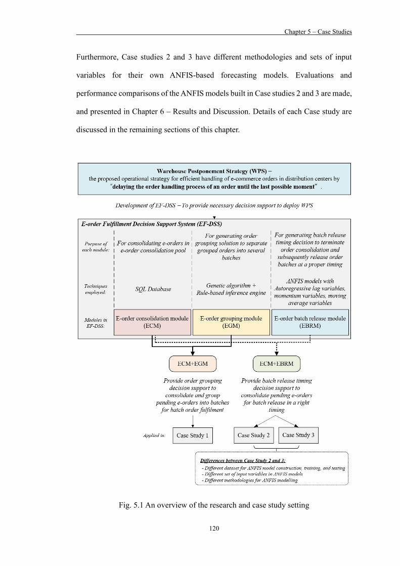
Chapter 5 – Case Studies
120
Furthermore, Case studies 2 and 3 have different methodologies and sets of input
variables for their own ANFIS-based forecasting models. Evaluations and
performance comparisons of the ANFIS models built in Case studies 2 and 3 are made,
and presented in Chapter 6 – Results and Discussion. Details of each Case study are
discussed in the remaining sections of this chapter.
Fig. 5.1 An overview of the research and case study setting

Chapter 5 – Case Studies
121
5.2 Case Study 1 – The Use of Hybrid GA-rule-based Approach for
Generating “How to Group” Decision Support
In Case study 1, the ECM and the EGM of the EF-DSS are deployed for assisting
the logistics service provider in consolidating and grouping the e-commerce orders
according to the proximity of the location of each SKU requested in the consolidated
orders. There are two essential features of the ECM and EGM provided for facilitating
the LSP in handling e-orders:
Facilitating the e-order consolidation process through the use of the e-order
consolidation pool in the ECM, and
Generating order grouping decision support for ease of fulfillment of
consolidated orders in the distribution centre.
In this section, the company background and problems encountered by the
company are described, followed by a discussion of the deployment of ECM and the
EGM.
5.2.1 Company Background and Existing Problems Encountered
The case company is a medium-sized Hong Kong-based logistics service
provider that has specialized in B2C e-commerce logistics and distribution services in
recent years. As China continues to drive cross-border growth, and its share of the
online cross-border market is expected to grow from 27% in 2015 to 40% in 2021
(Forrester Research, 2016b), the developing trend of e-commerce in China has created
a golden opportunity in recent years for logistics practitioners in Hong Kong and
within the Pearl River Delta region to grasp a large part of the e-commerce pie by
transforming their traditional B2B logistics businesses into e-commerce logistics
businesses. This can be achieved by providing total e-logistics solutions so that e-

Chapter 5 – Case Studies
122
retailers can concentrate on their core business by outsourcing the entire e-order
fulfilment, including e-commerce last-mile delivery operations, to logistics service
providers.
In view of the emerging trend of the e-commerce business, the company started
opening the e-commerce logistics business line in 2012. However, the company faces
enormous challenges in the e-commerce logistics business not only due to the tight
handling requirements of e-commerce orders, in which it is becoming popular for e-
retailers to guarantee 24-to-48-hour delivery to customers, but is also affected by the
internal inefficiency of e-order handling and processing. The challenges are generic
across the industry and are thus faced by the case company, and include:
(i) Heavy workload of warehouse operators in fulfilling the orders in a timely
manner
(ii) An increasing frequency of picking and packing wrong items
Both of these problems result from the irregular arrival of e-orders as online
customers can place orders at any time via the Internet. Another reason is due to the
fact that each B2C customer order involve a relatively large number of various types
of SKUs. This results in a higher chance of inaccurate order fulfilment considering the
large number of fragmented e-orders that are required to be fulfilled within a limited
time.
In view of the operating inefficiency in managing their e-commerce business, the
ECM and EGM of the EF-DSS are implemented in the case company with an
implementation roadmap as illustrated below, which highlights the essential stages of
development for the proposed system to function in a production environment.
Chapter 5 – Case Studies
123
5.2.2 Deployment of the ECM and EGM
The implementation procedures can be divided into four phases: (i) Cloud
database development, (ii) Customization of GA mechanism and rule-based inference
engine, and (iii) Front-end user interface development.
(i) Development of database and E-order consolidation pool
A database and an e-order consolidation pool are built in accordance with the
operating parameters and logistics orders that the company handle. As discussed in
Chapter 4 – Implementation procedures of the system, any system implementation can
be done only after a comprehensive user requirement study. Therefore, based on the
user requirement study, the database of the EF-DSS built for the company has the types
of data shown in Table 5.1.
As logistics orders of the company are received from the e-commerce online
retail sites, the retrieval and consolidation of an order therefore requires a cloud
database integrated into a web app for real time data retrieval and processing. A web
app, which consists of a series of web pages, is constructed in Hypertext Mark-up
Language (HTML) and is designed for the customer service staff of the company to
retrieve e-orders and allocate the e-orders to the e-order consolidation pool. Any action
made by the users on the web pages triggers an update on the cloud database of EF-
DSS. The database of EF-DSS is the information repository for collecting, storing and
sorting two types of data: (i) delivery order details, which are received in real time
directly from end consumers, and (ii) the basic settings of the e-fulfilment center,
which are static information preliminarily stored in the cloud database for retrieval.
The details of these two major types of data stored in the cloud database are displayed
in Table 5.1.

Chapter 5 – Case Studies
124
The major data processing operations in this module includes database query
processing, data sorting and display. For database query processing, essential data as
shown in Table 5.1 for insert, view, edit, delete and update can be performed in the UI
of the EF-DSS through a set of structure query language (SQL) statements designed
and stored in the SQL database. For data sorting and display, the operation is done
automatically in the back-end of the database so that all retrieved e-orders are
aggregated and sorted by stock-keeping units (SKUs), disregarding which particular
SKUs are fulfilling which customer order. With the rearranged order information, as
depicted in Fig. 5.2, a list of items to be processed in the e-fulfilment center is
displayed in the UI of the EF-DSS, which serves as the input of the subsequent module
for e-order grouping and resource allocation decision support.
Table 5.1. Types of data stored and collected in the database for the case company
Types of data for collection and storage in database:
(iii) Customer order details
Details Data type
Order number Numeric
SKU number Numeric
Total quantity of each SKU Numeric
Total weight of each SKU Numeric
Delivery location String
(iv) Initial setting of e-fulfilment centers Storage location setting (Zone and bin level) String
Travel distance between each bin location Numeric
Storage location of each SKU String
Equipment master String

Chapter 5 – Case Studies
125
Fig. 5.2. The underlying e-order information processing logic in ECM
With the database and e-order consolidation pool built for collecting, processing
e-order information and displaying the collected e-orders pending processing, the
logistics order processing flow is re-engineered by allowing users to control when
pending orders are ready for batch release to the warehouse department so as to
perform the order fulfilment operations. The centralized relational database sorts the
received orders by SKUs so that the SKUs to be handled in the e-fulfilment centers
are grouped for ease of actual processing. Figs. 5.3 and 5.4 show respectively the
storage area of the e-fulfilment centers of the case company where order picking
operations take place, and the computer terminal for the display and consolidation of
e-orders.
Fig. 5.3. Order picking operations in storage bin locations of e-fulfilment centers
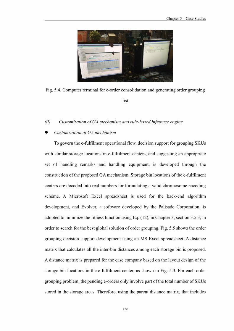
Chapter 5 – Case Studies
126
Fig. 5.4. Computer terminal for e-order consolidation and generating order grouping
list
(ii) Customization of GA mechanism and rule-based inference engine
Customization of GA mechanism
To govern the e-fulfilment operational flow, decision support for grouping SKUs
with similar storage locations in e-fulfilment centers, and suggesting an appropriate
set of handling remarks and handling equipment, is developed through the
construction of the proposed GA mechanism. Storage bin locations of the e-fulfilment
centers are decoded into real numbers for formulating a valid chromosome encoding
scheme. A Microsoft Excel spreadsheet is used for the back-end algorithm
development, and Evolver, a software developed by the Palisade Corporation, is
adopted to minimize the fitness function using Eq. (12), in Chapter 3, section 3.5.3, in
order to search for the best global solution of order grouping. Fig. 5.5 shows the order
grouping decision support development using an MS Excel spreadsheet. A distance
matrix that calculates all the inter-bin distances among each storage bin is proposed.
A distance matrix is prepared for the case company based on the layout design of the
storage bin locations in the e-fulfilment center, as shown in Fig. 5.3. For each order
grouping problem, the pending e-orders only involve part of the total number of SKUs
stored in the storage areas. Therefore, using the parent distance matrix, that includes

Chapter 5 – Case Studies
127
all inter-bin distances, is unnecessary. In this regard, a sorting algorithm, which is
developed using Visual Basic for Applications (VBA), a programming language that
automate tasks in MS Excel, is built for extracting the required inter-bin distances from
the parent distance matrix to form a child distance matrix. The programming code for
the sorting algorithm is shown in Fig. 5.6.
Fig. 5.5. Order grouping decision support development using GA
Customization of the rule-based inference engine
An appropriate set of operating guidelines and order handling equipment are
suggested through a rule-based inference engine for each of the e-order grouping
solutions generated from the GA mechanism. A rule-based inference engine is adopted
for ease of storing and manipulating human knowledge so as to interpret order
grouping information in a useful way. The engine is customized for the case company
based on the current throughput volume and resource availability for e-order
fulfilment operations in the e-fulfilment center. Three parameters are identified as the
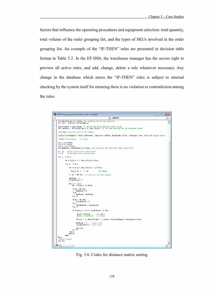
Chapter 5 – Case Studies
128
factors that influence the operating procedures and equipment selection: total quantity,
total volume of the order grouping list, and the types of SKUs involved in the order
grouping list. An example of the “IF-THEN” rules are presented in decision table
format in Table 5.2. In the EF-DSS, the warehouse manager has the access right to
preview all active rules, and add, change, delete a rule whenever necessary. Any
change in the database which stores the “IF-THEN” rules is subject to internal
checking by the system itself for ensuring there is no violation or contradiction among
the rules.
Fig. 5.6. Codes for distance matrix sorting

Chapter 5 – Case Studies
129
Table 5.2. Example rules applied in the case company
“IF” condition “THEN” Action Example rules for operating guidelines
Quantity is more than 50
Double check if the quantity picked for each SKU is correct at the end of operation
Volume is more than 20 kg
Reserve lower space for heavier item
Types of SKUs is more than 5
Pick up item separation tool for separating different SKUs;
Example rules for equipment selection Volume is 26-50 kg Use Multi-Storey Trolley for separation of different SKUs
Volume is more than 50 kg
Use Lifter
(iii) Front-end user interface development
A front-end user interface (UI) serving as the presentation and interaction tier for
users is designed, as shown in Figs. 5.7 and 5.8. It integrates the cloud database, back-
end GA mechanism and rule-based inference engine, so that users are able to
conveniently view the newly received e-orders which are retrieved from the Intranet
and stored in the cloud database; obtain decision support from the GA mechanism
regarding how the required SKUs from the pending e-orders are to be grouped for
batch processing in e-fulfilment centers; and receive suggestions from the rule-based
inference engine regarding the equipment and handling procedures of each order
grouping list generated in the GA mechanism. The EF-DSS is a web-based application
so that users can login to the system via the Internet. The Customer Service department
can decide when to stop the consolidation of e-orders and start initiating the EF-DSS
so as to generate order grouping suggestions, as shown in Fig. 5.8. The suggested
outputs can then be exported to other formats for modification or printed for the
warehouse department to execute accordingly. The warehouse department can modify

Chapter 5 – Case Studies
130
or add particular information to the EF-DSS, including the available material handling
equipment, operating guidelines for different types of e-orders and the storage location
of SKUs, so that the database is up-to-date and the decision support provided by EF-
DSS is feasible.
Fig. 5.7. User interfaces of EF-DSS – Order consolidation and grouping
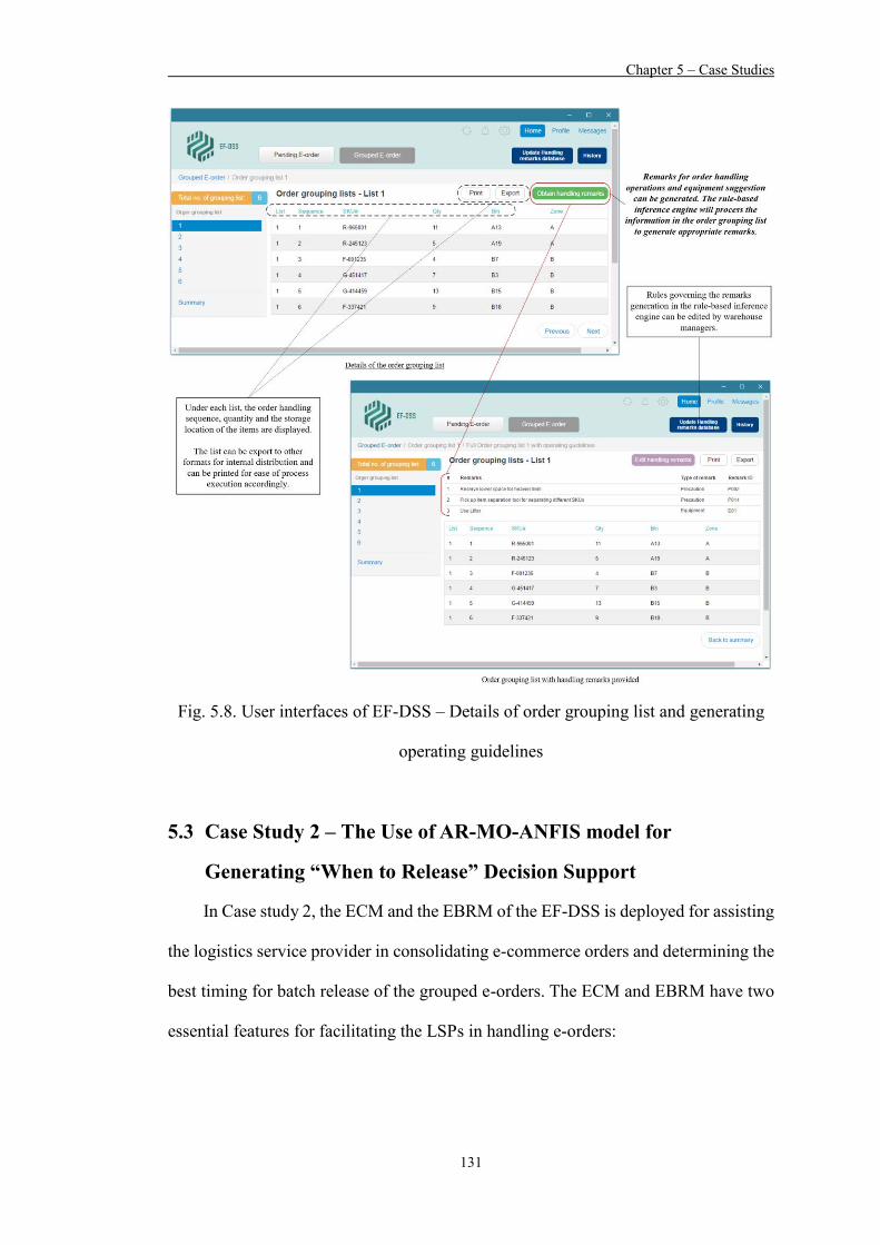
Chapter 5 – Case Studies
131
Fig. 5.8. User interfaces of EF-DSS – Details of order grouping list and generating
operating guidelines
5.3 Case Study 2 – The Use of AR-MO-ANFIS model for
Generating “When to Release” Decision Support
In Case study 2, the ECM and the EBRM of the EF-DSS is deployed for assisting
the logistics service provider in consolidating e-commerce orders and determining the
best timing for batch release of the grouped e-orders. The ECM and EBRM have two
essential features for facilitating the LSPs in handling e-orders:
Chapter 5 – Case Studies
132
Facilitating the e-order consolidation process through the use of the e-order
consolidation pool in the ECM, and
Generating batch release decision support for predicting the e-order arrival rate
in the coming period, thereby realizing the remaining time for them to continue
consolidating e-commerce orders until terminating the order consolidation
process and subsequently releasing the pending orders for immediate processing.
In this section, the company background and problems encountered by the
company are described, followed by a discussion of the deployment of ECM and the
EBRM.
5.3.1 Company Background and Existing Problems Encountered
The case company in this case study is a Hong Kong based logistics service
provider specialized in providing a wide range of logistics and transportation services
for cross-border shipments. With the emerging trend of e-commerce business, the
company started handling e-commerce shipments in 2014. However, due to the great
difference in the operating procedures and requirements in handling e-commerce
shipments as compared to traditional cross-border shipments, where e-commerce
orders were received at a much higher frequency and in smaller lot sizes, the company
has been struggling to sustain the e-commerce business, and is desperate to expand the
e-commerce logistics business by 2020. However, the following problems have been
faced by the company for a long time, which heavily affect the order handling
efficiency:
(i) Difficulty in resource allocation for order picking – Due to the high frequency
in receiving delivery orders from e-commerce customers, the company found

Chapter 5 – Case Studies
133
it difficult to assign human resources to pick the orders. The utilization rate of
the warehouse worker is therefore increasing, which gradually becomes a
bottleneck in the entire warehouse operations.
(ii) Increase in travelling distance of warehouse workers which is deemed
unnecessary – Instead of picking orders in a large batch and shipping large
volume orders as single shipment, e-commerce orders are picked, packed and
delivered in a smaller volume but at a higher frequency. Therefore, warehouse
workers are required to visit the same or nearby storage locations of the
warehouse repeatedly over the whole day in order to pick the orders.
In an attempt to rectify these problems, the ECM and the EBRM of EF-DSS are
deployed in the distribution centre of the company to assist them in handling e-
commerce shipments more efficiently by means of developing a warehouse
postponement strategy that groups the orders for batch picking and processing at the
most appropriate timing.
5.3.2 Deployment of the ECM and EBRM
The implementation procedures are divided into four phases: (i) Database
development, (ii) Identification of cut-off review cycle time and ANFIS model
construction, training and testing, (iii) “When to release” algorithm development and
implementation, and (iv) Front-end user interface development. In particular, in the
second phase, the ANFIS model construction methodology for Case studies 2 and 3
are different, for the sake of undertaking comprehensive testing to justify which
methodology is more suitable in predicting the e-order arrival. Details of each phase
of system implementation are discussed below.

Chapter 5 – Case Studies
134
(i) Database development
Data collection is conducted to build the cloud database and server. The details
of over 500 historical e-commerce order receiving pre-bookings are collected and
analyzed for the construction of a relational database, a core component of the ECM
in EF-DSS. With the database and e-order consolidation pool, the ECM collects
historical online sales data and receives e-commerce orders from the cloud. Other
relevant data, such as the real time availability of order pickers and order handling
equipment, etc., are also retrieved from the e-commerce sales platform and transmitted
to the cloud database of the EF-DSS. Any update of the information, such as receiving
a new order from an online customer, will be synchronized with the cloud database of
the EF-DSS. The cloud database also serves an e-order consolidation pool to
consolidate the incoming e-orders for subsequently releasing them in a batch.
The major data processing operations in this module include database query
processing, data sorting and data display, which is similar to the database development
discussed in Case study 1. Similarly, with a set of structure query language (SQL)
statements designed and stored in the SQL database, the EF-DSS enables users to view
and edit the information in the system user interfaces. Back-end data sorting and order
detail aggregation are performed, so that the grouped e-orders are aggregated and
sorted according to the stock-keeping units (SKUs), rather than the order number. This
e-order information processing logic in the ECM is the same as depicted in Fig. 5.2 in
Case study 1. The processed data in this module then serves as the inputs values of the
ANFIS model in EBRM of the EF-DSS.
Chapter 5 – Case Studies
135
(ii) Identification of cut-off review cycle time and ANFIS model construction,
training and testing
The conceptual framework for ANFIS model construction for this case study is
presented in Fig. 5.9. Typically, to gain brand exposure and expand the target customer
segments, e-retailers list their product lineup on various e-commerce sales channels,
such as Tmall, Amazon, JD.com, etc., so that online customers can place orders in
these sales channels. As the case company had agreements with several e-retailers to
handle the outsourced order fulfillment activities, such as stocking of goods, order
pick and pack, and order delivery operations, the details of online e-commerce orders
placed by the end consumers are transmitted to the case company by the e-retailers.
Before the deployment of the EF-DSS, these e-orders are processed immediately
upon arrival at the company. With the deployment of EF-DSS, the ECM consolidates
the e-orders in the e-order consolidation pool until reaching the best batch release
timing. To identify the best batch release timing to terminate the consolidation process
of the e-orders and release the pending e-orders for the operators in the distribution
centre to perform the subsequent order fulfillment process, the EBRM first predicts
the arrival of e-orders for the next period. A single ANFIS model is used for predicting
the arrival of e-orders, regardless of which e-retailer the e-order belongs to, as shown
in Fig 5.9. Then, using the predicted e-order arrival figure, a “When to release”
algorithm is adopted to compute the remaining time in which the company could still
consolidate e-orders.
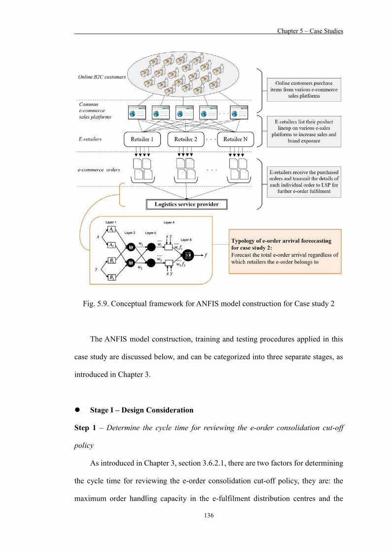
Chapter 5 – Case Studies
136
Fig. 5.9. Conceptual framework for ANFIS model construction for Case study 2
The ANFIS model construction, training and testing procedures applied in this
case study are discussed below, and can be categorized into three separate stages, as
introduced in Chapter 3.
Stage I – Design Consideration
Step 1 – Determine the cycle time for reviewing the e-order consolidation cut-off
policy
As introduced in Chapter 3, section 3.6.2.1, there are two factors for determining
the cycle time for reviewing the e-order consolidation cut-off policy, they are: the
maximum order handling capacity in the e-fulfilment distribution centres and the

Chapter 5 – Case Studies
137
average number of orders (in kg) received per hour. Through the historical order
arrival figures and the information regarding the order handling resource capacity
provided by the management, the cycle time (“the period”) for the company is set to
be 2 hours. In other words, at the end of each “period”, the management uses the EF-
DSS to predict the e-order arrival of the next “period”, so as to realize how much time
is left for them to release the pending e-orders in a batch.
Step 2 – Identify the input and output variables in the ANFIS models
As the cycle time is set as two hours in Step 1, the output of the ANFIS model in
this case study, Qd(t+1), denotes the predicted arrival of the e-orders (in kg) in the
upcoming period t+1 in the current day d, i.e. the coming two hours. In this case study,
two input variables are selected as the prediction indicators of the e-order arrival in
the new 2-hour horizon, they are: the previous e-order arrival figures and the volatility
of e-order arrival. This is the first study attempting to forecast the arrival of e-
commerce order volume for managing the fluctuation of throughput in supply chains,
as well as forecasting the subject through the integration of autoregressive models and
ANFIS. Detailed explanations of the input variables are provided below.
(1) Actual n-period e-order arrival: Actual e-order arrival in the previous n periods,
i.e. period t, t-1, t-2, …, t-n, are considered as essential indicators for predicting
the e-order arrival figure at the upcoming period t+1. The identification of the
lag length for a time series is especially essential. To address this issue and to
identify the appropriate number of lag periods n that is the most fitting for the
experimental dataset, an autoregressive (AR) model is formulated and estimated
with the use of EViews software package. By using the least square method, we
initially select 10 lag variables, i.e. Qd(t-n), where n=0, 1, …, 9, for testing. If the

Chapter 5 – Case Studies
138
p-value is less than the 0.05 significance level, then the null hypothesis is rejected.
A four-week data set, which consists of a total of 336 observations of the e-order
arrivals in each two-hour interval, are extracted. The first two-thirds of the
observations, i.e. 223 observations, are selected to estimate and test the AR
models. The lag test results, as shown in Fig. 5.10, reveal that both the one-order
AR model (AR(1)) and the seven-order AR model (AR(7)) give the lowest p-
values, which are both lower than 0.05. This indicates that both the inclusion of
one lag variable and seven lag variables are the most appropriate AR model
settings for the prediction of the e-order arrival figures. We then use the AR(1)
and AR(7) models to forecast the remaining one-third of the observations and
compare with the actual e-order arrival figures. Table 5.3 shows the test results
of the AR(1) and AR(7) models measured by the root mean squared error (RMSE),
and the coefficient of determinations (R2), which are respectively measured by:
RMSE = √∑ (𝑃𝑖−𝑦𝑖)2𝑛
𝑖=1
𝑛 (33)
𝑅2 = 1 −𝑆𝑆𝑟𝑒𝑠
𝑆𝑆𝑡𝑜𝑡 (34)
where yi and Pi are respectively the actual arrival of e-order and predict arrival of
e-order (in terms of weight in kg) at period t, and n is the number of data patterns
in the independent data set. SSres and SStot respectively represent the residual sum
of square and the total sum of squares, calculated by:
𝑆𝑆𝑟𝑒𝑠 = ∑ (𝑃𝑖 − �̅�)2𝑛𝑖=1 (35)
𝑆𝑆𝑡𝑜𝑡 = ∑ (𝑦𝑖 − �̅�)2𝑛𝑖=1 (36)
where �̅� is the mean of the actual data. From Table 2, the AR(7) model performs
slightly better in forecasting the e-order arrival than AR(1), as AR(7) gives a

Chapter 5 – Case Studies
139
slightly lower values of RMSE and R2. However, if the AR(7) model is to be
adopted, a total of seven lag variables will be included in the ANFIS model. This
will severely increase the computation time and requirements, as well as generate
a large number of If-then rules in the inference engine of the ANFIS model.
Therefore, taking these drawbacks into consideration in the ANFIS modelling,
the AR(1) model is selected over the AR(7) model. In other words, the output
variable Qd(t+1), is forecast based on only one lag variable Qd(t-n), for n = 0.
(2) Volatility of previous e-order arrival: The volatility of the previous e-order
arrival (momentum) is an essential indicator of the trend of the time-series-based
e-order arrival. This indicator has been used to predict stock prices. Tanaka-
Yamawaki & Tokuoka (2007) introduced one and two-order momentum as one
of the technical indicators of intra-day stock price prediction. Chang et al. (2011)
also introduced one and two-order momentum for forecasting the stock prices.
Thus, this study considers both one and two-order momentum of the e-order
arrival as the input variables. For the current period t, one-order momentum,
Mo(t), and two-order momentum, Mo(t-1), of e-order arrival are respectively
calculated by:
𝑀𝑜(𝑡) = 𝑄𝑑(𝑡) − 𝑄𝑑(𝑡 − 1) (37)
𝑀𝑜(𝑡 − 1) = 𝑄𝑑(𝑡 − 1) − 𝑄𝑑(𝑡 − 2) (38)
Two separate ANFIS models, AR(1)MO(1) model and AR(1)MO(2), are built,
one with one-order momentum as the input variable, and the other with both one-
order and two-order momentum as the input variables. Evaluation and error
analysis are performed to justify whether the inclusion of two-order momentum is
suitable for the prediction of e-order arrival.

Chapter 5 – Case Studies
140
Fig. 5.10. Lag test for identifying the number of lag length n
Table 5.3. Test results of AR(1) and AR(7) model
RMSE R2 AR(1) model 15.43 0.52 AR(7) model 13.12 0.69
Step 3 – Select and extract dataset for model training and testing
A four-week real production data set from the beginning of January of 2018 is
gathered and extracted from the case company’s distribution centre where e-order
fulfilment operations take place. With the management specifying a preferred cut-off
review cycle of two working hours, the data sets are pre-processed and converted into
useful input values for the proposed ANFIS models. Table 5.4 shows a data set
regarding the actual four-week e-order arrival in a two-hour interval (measured by kg),
which are used for performing lag testing to identify the appropriate number of lag
periods n, as discussed in Step 1. In addition, in order to validate the neural system,
the 4-week data set, comprised of 336 data pairs in total, is split into training and
testing data sets. Usually, the training data set, contains 70% or 90% of all data and
the remaining data serves as the testing data set (Sánchez et al., 2007), is used to train
and build the adaptive network, whereas the testing data set is used to determine if any
over fitting of the model occurs during training.
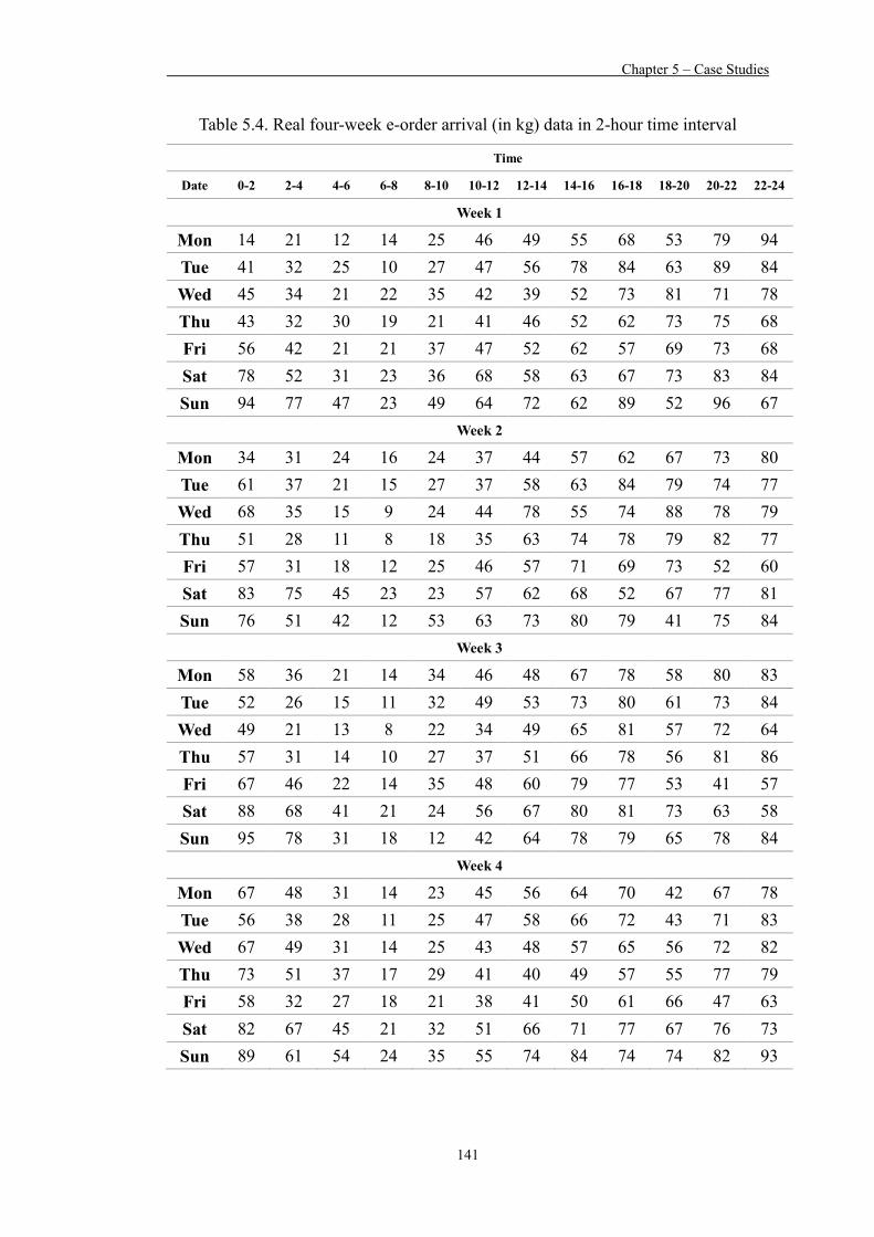
Chapter 5 – Case Studies
141
Table 5.4. Real four-week e-order arrival (in kg) data in 2-hour time interval
Time
Date 0-2 2-4 4-6 6-8 8-10 10-12 12-14 14-16 16-18 18-20 20-22 22-24
Week 1 Mon 14 21 12 14 25 46 49 55 68 53 79 94 Tue 41 32 25 10 27 47 56 78 84 63 89 84 Wed 45 34 21 22 35 42 39 52 73 81 71 78 Thu 43 32 30 19 21 41 46 52 62 73 75 68 Fri 56 42 21 21 37 47 52 62 57 69 73 68 Sat 78 52 31 23 36 68 58 63 67 73 83 84 Sun 94 77 47 23 49 64 72 62 89 52 96 67
Week 2 Mon 34 31 24 16 24 37 44 57 62 67 73 80 Tue 61 37 21 15 27 37 58 63 84 79 74 77 Wed 68 35 15 9 24 44 78 55 74 88 78 79 Thu 51 28 11 8 18 35 63 74 78 79 82 77 Fri 57 31 18 12 25 46 57 71 69 73 52 60 Sat 83 75 45 23 23 57 62 68 52 67 77 81 Sun 76 51 42 12 53 63 73 80 79 41 75 84
Week 3 Mon 58 36 21 14 34 46 48 67 78 58 80 83 Tue 52 26 15 11 32 49 53 73 80 61 73 84 Wed 49 21 13 8 22 34 49 65 81 57 72 64 Thu 57 31 14 10 27 37 51 66 78 56 81 86 Fri 67 46 22 14 35 48 60 79 77 53 41 57 Sat 88 68 41 21 24 56 67 80 81 73 63 58 Sun 95 78 31 18 12 42 64 78 79 65 78 84
Week 4 Mon 67 48 31 14 23 45 56 64 70 42 67 78 Tue 56 38 28 11 25 47 58 66 72 43 71 83 Wed 67 49 31 14 25 43 48 57 65 56 72 82 Thu 73 51 37 17 29 41 40 49 57 55 77 79 Fri 58 32 27 18 21 38 41 50 61 66 47 63 Sat 82 67 45 21 32 51 66 71 77 67 76 73 Sun 89 61 54 24 35 55 74 84 74 74 82 93

Chapter 5 – Case Studies
142
Step 4 – Define the universe of disclosure for each input parameter
To achieve the best result generated from the ANFIS model, system parameter
modifications are critical. In the MATLAB’s ANFIS editor, different types of
membership functions (MFs), such as triangular (Tri), trapezoidal (Trap), generalized
bell (Gbell), Gaussian curve (Guass), Gaussian combination, Π-shaped, difference
between two sigmoid functions, and product of two sigmoid functions, are available
for selection. In addition, the number of MFs for each input, and the types of output
MFs (either constant or linear) can also be modified. Due to the large number of
possible combinations of the parameter settings of the ANFIS model, the best
combination of the ANFIS model needs to be identified. The model structure of
AR(1)MO(1) and AR(1)MO(2), and a summary of the training parameters of the both
models is presented and shown in Figs. 5.11, and 5.12 and Table 5.5 respectively.
Fig. 5.11. AR(1)MO(1) model structure
Fig. 5.12. AR(1)MO(2) model structure
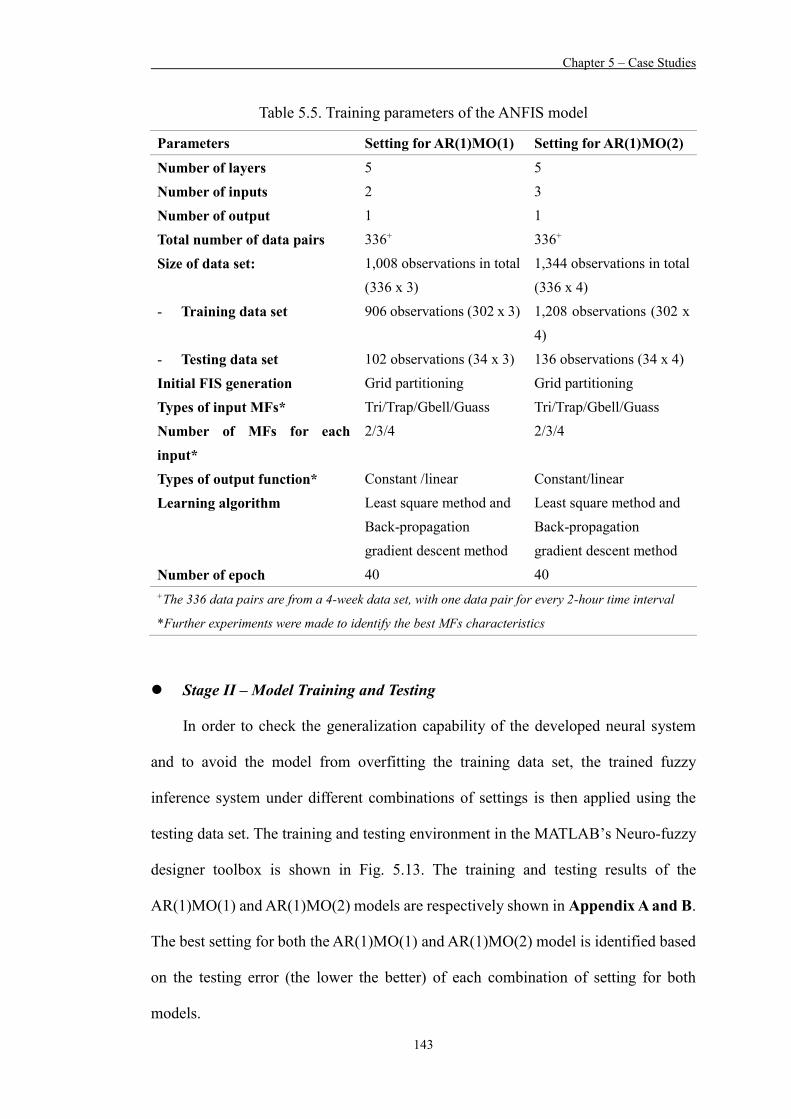
Chapter 5 – Case Studies
143
Table 5.5. Training parameters of the ANFIS model
Parameters Setting for AR(1)MO(1) Setting for AR(1)MO(2)
Number of layers 5 5 Number of inputs 2 3 Number of output 1 1 Total number of data pairs 336+ 336+ Size of data set: 1,008 observations in total
(336 x 3) 1,344 observations in total (336 x 4)
- Training data set 906 observations (302 x 3) 1,208 observations (302 x 4)
- Testing data set 102 observations (34 x 3) 136 observations (34 x 4) Initial FIS generation Grid partitioning Grid partitioning Types of input MFs* Tri/Trap/Gbell/Guass Tri/Trap/Gbell/Guass Number of MFs for each input*
2/3/4 2/3/4
Types of output function* Constant /linear Constant/linear Learning algorithm Least square method and
Back-propagation gradient descent method
Least square method and Back-propagation gradient descent method
Number of epoch 40 40 +The 336 data pairs are from a 4-week data set, with one data pair for every 2-hour time interval
*Further experiments were made to identify the best MFs characteristics
Stage II – Model Training and Testing
In order to check the generalization capability of the developed neural system
and to avoid the model from overfitting the training data set, the trained fuzzy
inference system under different combinations of settings is then applied using the
testing data set. The training and testing environment in the MATLAB’s Neuro-fuzzy
designer toolbox is shown in Fig. 5.13. The training and testing results of the
AR(1)MO(1) and AR(1)MO(2) models are respectively shown in Appendix A and B.
The best setting for both the AR(1)MO(1) and AR(1)MO(2) model is identified based
on the testing error (the lower the better) of each combination of setting for both
models.

Chapter 5 – Case Studies
144
Fig. 5.13. ANFIS model training and testing environment in MATLAB’s Neuro-
fuzzy designer toolbox
Stage III – Performance Evaluations
With the best setting respectively obtained for both AR(1)MO(1) and
AR(1)MO(2), these developed models are then compared with an autoregressive
integrated moving average (ARIMA) model for further performance validation.
The ARIMA model
In the ARIMA model, the predicted value of a variable is assumed to be a linear
function of several past p observations and q random errors. A stationary ARIMA(p,q)
model captures dependencies in the series in two parts, autoregressive (AR) and
moving average (MA), in the form:
y(t) = 𝑎0 + 𝑎1𝑦(𝑡 − 1) + 𝑎2𝑦(𝑡 − 2) + ⋯ + 𝑎𝑝𝑦(𝑡 − 𝑝)
+𝑒(𝑡) + 𝑏1𝑒(𝑡 − 1) + 𝑏2𝑒(𝑡 − 2) + ⋯ + 𝑏𝑞𝑒(𝑡 − 𝑞) (39)

Chapter 5 – Case Studies
145
where the autoregressive part is a linear combination of the past p observations y(t-
1), …, y(t-p), weighted by p linear coefficients a1, …, ap, and a constant term a0. The
moving average part is a linear combination of the past q error terms e(t-1), …, e(t-q),
weighted by q linear coefficients b1, …, bp, and the current error term e(t). The error
terms are assumed to be independently and identically distributed with a mean of zero
and a constant variance of σ2. Seasonal autoregressive (SAR) and seasonal moving
average (SMA) term, r and s, may also be added to the ARIMA model, in case of
having a periodic time series pattern.
To compare the model performance among the ANFIS models of AR(1)MO(1),
AR(1)MO(2), and the ARIMA model, the root-mean square error (RMSE), mean
absolute deviation (MAD), and mean absolute percentage error (MAPE) are used,
which are respectively given by Eq. (25), (26), and (27), as shown in Section 3.6.2.3
on p. 98.
(iii) “When to release” algorithm development and implementation
With the developed ANFIS model with the best model setting through model
training and testing, the output of the ANFIS model in EBRM of the EF-DSS, i.e. the
predicted arrival of e-commerce orders in the upcoming period, measured by the
weight in kg, is then used as one of the variables to generate decision support for
logistics practitioners to adjust the cut-off frequency of releasing the grouped orders
for actual order picking operations in a batch. To compute the cut-off time of the e-
order grouping, the proposed approach in the EF-DSS suggests taking the maximum
order handling capacity in the distribution centre into consideration, as discussed in
Chapter 3, Section 3.6.3.
The maximum order handling capacity, Qmax, is obtained by identifying the total
weight that can be handled by the resources for order handling, such as equipment and

Chapter 5 – Case Studies
146
the order pickers, which are currently idle and available for performing picking
operations of the e-orders. With the known constant value of Qmax, EF-DSS is able to
automatically generate the cut-off time, denoted as Tfinal, with the notation definitions
as shown in Table 5.6 (the same as in Section 3.6.3) and the underlying calculations
as described below.
In order to avoid any potential over-utilization of the order handling resources,
especially human resources, the maximum allowable order handling capacity (Qmax)
is multiplied by a constant factor k (in %) to give an adjusted order handling capacity
(Qadjusted). For this case study, based on discussions with the management, the value of
k is set to be 0.8. To obtain the current remaining order handling capacity (Qremaining),
the adjusted order handling capacity is subtracted by the total weight of pending orders
in the e-order consolidate pool (Qcurrent), which is expressed as:
𝑄𝑎𝑑𝑗𝑢𝑠𝑡𝑒𝑑 = 𝑄𝑚𝑎𝑥 × 𝑘 (40)
𝑄𝑟𝑒𝑚𝑎𝑖𝑛𝑖𝑛𝑔 = 𝑄𝑎𝑑𝑗𝑢𝑠𝑡𝑒𝑑 − 𝑄𝑐𝑢𝑟𝑟𝑒𝑛𝑡 (41)
The predicted e-order arrival rate per minute (Qt) is computed by dividing the
predicted weight of the incoming e-orders in the upcoming period t+1 (Qd(t+1), the
output of the ANFIS model), by the total duration in the specified period (in minutes)
(n). It is expressed as:
𝑄𝑡 =𝑄𝑑(𝑡+1)
𝑛 (42)
The optimal cut-off time for batch order release can then be computed by dividing Eq.
(41) by Eq. (42), that is:
𝑇𝑜𝑝𝑡𝑖𝑚𝑎𝑙 =𝑄𝑟𝑒𝑚𝑎𝑖𝑛𝑖𝑛𝑔
𝑄𝑡 (43)
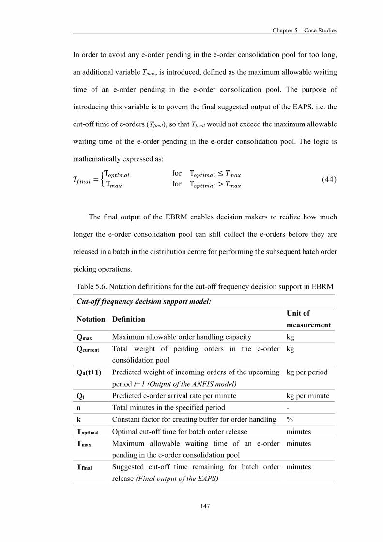
Chapter 5 – Case Studies
147
In order to avoid any e-order pending in the e-order consolidation pool for too long,
an additional variable Tmax, is introduced, defined as the maximum allowable waiting
time of an e-order pending in the e-order consolidation pool. The purpose of
introducing this variable is to govern the final suggested output of the EAPS, i.e. the
cut-off time of e-orders (Tfinal), so that Tfinal would not exceed the maximum allowable
waiting time of the e-order pending in the e-order consolidation pool. The logic is
mathematically expressed as:
𝑇𝑓𝑖𝑛𝑎𝑙 = {T𝑜𝑝𝑡𝑖𝑚𝑎𝑙 for T𝑜𝑝𝑡𝑖𝑚𝑎𝑙 ≤ 𝑇𝑚𝑎𝑥
T𝑚𝑎𝑥 for T𝑜𝑝𝑡𝑖𝑚𝑎𝑙 > 𝑇𝑚𝑎𝑥 (44)
The final output of the EBRM enables decision makers to realize how much
longer the e-order consolidation pool can still collect the e-orders before they are
released in a batch in the distribution centre for performing the subsequent batch order
picking operations.
Table 5.6. Notation definitions for the cut-off frequency decision support in EBRM
Cut-off frequency decision support model:
Notation Definition Unit of measurement
Qmax Maximum allowable order handling capacity kg Qcurrent Total weight of pending orders in the e-order
consolidation pool kg
Qd(t+1) Predicted weight of incoming orders of the upcoming period t+1 (Output of the ANFIS model)
kg per period
Qt Predicted e-order arrival rate per minute kg per minute n Total minutes in the specified period - k Constant factor for creating buffer for order handling % Toptimal Optimal cut-off time for batch order release minutes Tmax Maximum allowable waiting time of an e-order
pending in the e-order consolidation pool minutes
Tfinal Suggested cut-off time remaining for batch order release (Final output of the EAPS)
minutes
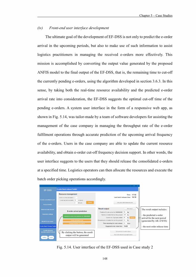
Chapter 5 – Case Studies
148
(iv) Front-end user interface development
The ultimate goal of the development of EF-DSS is not only to predict the e-order
arrival in the upcoming periods, but also to make use of such information to assist
logistics practitioners in managing the received e-orders more effectively. This
mission is accomplished by converting the output value generated by the proposed
ANFIS model to the final output of the EF-DSS, that is, the remaining time to cut-off
the currently pending e-orders, using the algorithm developed in section 3.6.3. In this
sense, by taking both the real-time resource availability and the predicted e-order
arrival rate into consideration, the EF-DSS suggests the optimal cut-off time of the
pending e-orders. A system user interface in the form of a responsive web app, as
shown in Fig. 5.14, was tailor-made by a team of software developers for assisting the
management of the case company in managing the throughput rate of the e-order
fulfilment operations through accurate prediction of the upcoming arrival frequency
of the e-orders. Users in the case company are able to update the current resource
availability, and obtain e-order cut-off frequency decision support. In other words, the
user interface suggests to the users that they should release the consolidated e-orders
at a specified time. Logistics operators can then allocate the resources and execute the
batch order picking operations accordingly.
Fig. 5.14. User interface of the EF-DSS used in Case study 2

Chapter 5 – Case Studies
149
5.4 Case Study 3 – The Use of AR-MO-MA-ANFIS model for
Generating “When to Release” Decision Support
In Case study 3, the ECM and the EBRM of the EF-DSS is deployed for assisting
the logistics service provider in consolidating e-commerce orders and determining the
best timing for batch release of the grouped e-orders. Same as in Case study 2, there
are two essential features of the ECM and EBRM provided for facilitating the LSP in
handling e-orders, they are:
Facilitating the e-order consolidation process through the use of the e-order
consolidation pool in the ECM, and
Generating batch release decision support for predicting the e-order arrival rate
in the coming period, thereby realizing the remaining time for them to continue
consolidating e-commerce orders until being terminated in the order
consolidation process and subsequently releasing the pending orders for
immediate processing.
As both Case studies 2 and 3 deployed the ECM and EBRM, the implementation
procedures of Case study 3 is the same as Case study 2, which are divided into four
phases: (i) Database development, (ii) Identification of cut-off review cycle time and
ANFIS model construction, training and testing, (iii) “When to release” algorithm
development and implementation, and (iv) Front-end user interface development. For
Phase 1, 3, and 4, the details of implementation are very similar. Therefore, they are
not covered in this section. However, in Phase 2 – Identification of cut-off review
cycle time and ANFIS model construction, training and testing, a more comprehensive
ANFIS model construction methodology is developed in this case study, for the sake
of undertaking more testing to justify which methodology is more suitable in
predicting the e-order arrival. Therefore, in this section, the company background and
Chapter 5 – Case Studies
150
problems encountered by the company are described, followed by a discussion of the
ANFIS construction framework, ANFIS training and testing procedures that have been
solely applied to this case study.
5.4.1 Company Background and Existing Problems Encountered
The case company in this case study is a Hong Kong-based logistics service provider
that started the outsource e-commerce order fulfillment in 2015. It is a third-party
logistics service provider, traditionally providing total logistics solutions including
freight management, warehouse management, value-added logistics services, project-
based cargo handling and local distribution of orders. Due to the growing trend of e-
commerce business, it started offering logistics solutions for e-commerce retailers in
2015, through providing door-to-door order receive and delivery, e-commerce order
consolidation and freight management, import and export declaration. In order to be
capable of handling a significant number of e-commerce orders, the company has an
80,000 sq. ft. warehouse designated for day-to-day receive and delivery of e-
commerce orders from retailers.
Due to the rapid expansion of the global e-commerce business, the throughput
rate of the e-fulfillment distribution centre of the company for e-commerce order
handling has been significantly increased since late 2015. With the drastic increase in
the number of daily orders to be handled in the warehouse, the company has been
facing several challenges which severely influence the warehouse operating efficiency
in e-commerce order fulfillment. These include:
(i) Overutilization of labor, particularly during receiving and put-away
operations – limited labor resources has become a major constraint in
maintaining the same degree of operating and handling efficiency, as e-

Chapter 5 – Case Studies
151
commerce orders involve more types of SKUs in comparison with traditional
orders.
(ii) Repetitive put-away operations being performed too frequently – Given the
irregular arrival of e-commerce orders at the inbound dock and a larger number
of fragmented orders as compared with traditional orders, put-away operations
are repeatedly undertaken throughout the working hours. Such operation
inefficiency at the inbound area consequently leads to delays in performing the
subsequent order fulfillment process especially outbound pick-and-pack and
delivery operations.
As a result, the retailers have urged the company to improve the standard of e-
commerce order fulfillment. In the light of this essential need to improve the
warehouse internal e-commerce order processing efficiency, the company has trial
launched EF-DSS to facilitate inbound operations of e-commerce orders.
5.4.2 Deployment of the ECM and EBRM
As suggested in Section 5.4, among the four phases of implementing ECM and
EBRM, i.e. (i) Database development, (ii) Identification of cut-off review cycle time
and ANFIS model construction, training and testing, (iii) “When to release” algorithm
development and implementation, and (iv) Front-end user interface development, the
discussion of this case study focuses on Phase 2 – Identification of cut-off review cycle
time and ANFIS model construction, training and testing.
The conceptual framework for ANFIS model construction in this case study is
presented in Fig. 5.15. Similar to the framework for Case study 2 (as shown in Fig.
5.9), e-retailers list their product lineup on various online sales platforms, allowing

Chapter 5 – Case Studies
152
online customers to make purchases at anytime and anywhere. In this case study, the
case company has partnership with three retailers. In other words, the case company
receives e-order arrivals only from these three retailers. In this regard, two typologies
are developed with different sets of ANFIS models for prediction:
Typology I – Forecasting the total e-order arrival by aggregating e-order arrival
from 3 retailers
This typology is the same as the typology adopted in Case study 2, in which
only one single ANFIS model is constructed for predicting the total e-order
arrival, regardless of which retailer the e-orders belong to. This approach is
comparatively straightforward but neglects the e-order arrival pattern of an
individual retailer.
Typology II – Separately forecasting the e-order arrival of each individual
retailer
This typology is specifically designed and applied to this case company as there
are only three retailers, who have partnership with the company, to outsource the
e-order fulfillment process. The idea of this typology is to construct three
different ANFIS models to forecast the e-order arrival patterns of each individual
retailer. By summing the predicted e-order arrival figures of each individual
retailer, the total predicted e-order arrival can be obtained. The case company can
also realize the e-order arrival of the next period. Additionally, this typology
allows the company to realize the e-order arrival behavior of an individual retailer.
Specialized or targeted operational strategies, such as resource re-allocation, can
also be formulated for better handling of incoming e-commerce orders.
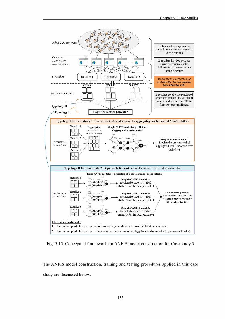
Chapter 5 – Case Studies
153
Fig. 5.15. Conceptual framework for ANFIS model construction for Case study 3
The ANFIS model construction, training and testing procedures applied in this case
study are discussed below.

Chapter 5 – Case Studies
154
Stage I – Design Consideration
Step 1 – Determine the cycle time for reviewing the e-order consolidation cut-off
policy
Same as Case study 2, two factors for determining the cycle time for reviewing
the e-order consolidation cut-off policy, i.e. the maximum order handling capacity in
the e-fulfilment distribution centres and the average number of orders (in kg) received
per hour, are considered. Through the historical order arrival figures and the
information regarding the order handling resource capacity provided by the
management, the cycle time (“the period”) for the company is set to be 3 hours. In
other words, at the end of each “period”, the management is going to use the EF-DSS
to predict the e-order arrival of the next “period”, so as to realize how much time is
left for them to release the pending e-orders in a batch.
Step 2 – Identify the input and output variables in the ANFIS models for both
typologies
As the cycle time is set as three hours in Step 1, the output of the ANFIS model
in this case study, Qd(t+1), denotes the predicted arrival of the e-orders (in kg) in the
upcoming period t+1 in the current day d, i.e. the coming three hours. In this case
study, other than the two input variables introduced in Case study 2, i.e. the previous
e-order arrival figures and the volatility of e-order arrival, a new input variable, i.e.
the n-period moving average, which is also discussed in Chapter 3, Section 3.6.2.1, is
added for further experiments to justify if the inclusion of moving average element
can provide a better predicting performance. Hence, three input variables are selected
as the prediction indicators of the e-order arrival in the new 3-hour horizon. Details of
each input variable are discussed below.

Chapter 5 – Case Studies
155
(1) Actual n-period e-order arrival: Actual e-order arrivals in the previous n
periods, i.e. period t, t-1, t-2, …, t-n, are considered as essential prediction
indicators for predicting the e-order arrival figure in the upcoming period t+1.
Same as in Case study 2, identifying the appropriate number of lag periods n that
is the most fitting for the experimental dataset is required. An autoregressive (AR)
model is formulated and estimated with the use of EViews software package. By
using the least squares method, we initially select 10 lag variables for each
reatailer’s dataset, i.e. Qd(t-n), where n=0, 1, …, 9, for testing. If the p-value is
less than the 0.05 significance level, then reject the null hypothesis. An eight-
week data set, which consists of a total of 448 observations of the e-order arrivals
in each three-hour interval, are extracted. The first two-thirds of the observations,
i.e. 298 observations, are selected to estimate and test the AR models. The lag
test results for the aggregated dataset in typology I and for each retailer’s dataset
in typology II are demonstrated:
Dataset for aggregated e-order arrival suggested in Typology I:
The lag test results, as shown in Fig. 5.16, reveal that both the one-order AR
model (AR(1)) and the eight-order AR model (AR(8)) give the lowest p-values,
which are both lower than 0.05. This indicates that both the inclusion of one lag
variable and eight lag variables are the most appropriate AR model settings for
the prediction of the e-order arrival figures. The AR(1) and AR(8) models are
then used to forecast the remaining one-third of the observations and compare
with the actual e-order arrival figures. Table 5.7 shows the test results of the AR(1)
and AR(8) models measured by the root mean squared error (RMSE) and the
coefficient of determinations (R2). From Table 5.7, the AR(8) model performs
better in forecasting the e-order arrival than AR(1), as AR(8) gives a lower value

Chapter 5 – Case Studies
156
of RMSE and R2. However, if the AR(8) model is to be adopted, a total of eight
lag variables will be included in the in an ANFIS model. This will severely
increase the computation time and requirements, as well as generate a large
number of If-then rules in the inference engine of the ANFIS model. Therefore,
taking these drawbacks into consideration in the ANFIS modelling, the AR(1)
model is selected over the AR(8) model. In other words, the output variable
Qd(t+1), is to be forecast based on only one lag variable Qd(t-n), for n = 0.
Fig. 5.16. Lag test for identifying the number of lag lengths n for the aggregated
dataset
Table 5.7. Test results of AR(1) and AR(8) model for aggregated dataset
RMSE R2 AR(1) model 46.74 0.43 AR(8) model 32.90 0.72
Dataset for retailer 1 in Typology II:
The lag test results, as shown in Fig. 5.17, reveal that both the one-order AR
model (AR(1)) and the eight-order AR model (AR(8)) give the lowest p-values,
which are both lower than 0.05. This indicates that the inclusion of one lag

Chapter 5 – Case Studies
157
variable and eight lag variables are the most appropriate AR model settings for
the prediction of the e-order arrival figures. The AR(1) and AR(8) model are then
used to forecast the remaining one-third of the observations and compare with
the actual e-order arrival figures. Table 5.8 shows the test results of the AR(1)
and AR(8) modeld measured by the root mean squared error (RMSE) and the
coefficient of determinations (R2). From Table 5.8, the AR(8) model performs
slightly better in forecasting the e-order arrival than AR(1), as AR(8) gives
slightly lower values of RMSE and R2. However, if the AR(8) model is to be
adopted, a total of eight lag variables will be included in the in an ANFIS model.
This will severely increase the computation time and requirements, as well as
generate a large number of If-then rules in the inference engine of the ANFIS
model. Therefore, taking these drawbacks into consideration in the ANFIS
modelling, the AR(1) model is selected over the AR(8) model. In other words,
the output variable Qd(t+1), is to be forecast based on only one lag variable Qd(t-
n), for n = 0.
Fig. 5.17. Lag test for identifying the number of lag lengths n for retailer 1

Chapter 5 – Case Studies
158
Table 5.8. Test results of AR(1) and AR(8) model for retailer 1
RMSE R2 AR(1) model 16.02 0.39 AR(8) model 12.20 0.65
Dataset for retailer 2 in Typology II:
Similarly, the lag test results for retailer 2, as shown in Fig. 5.18, reveal that both
the one-order AR model (AR(1)) and the four-order AR model (AR(4)) give the
lowest p-values, which are both lower than 0.05. Then, the AR(1) and AR(4)
models are used to forecast the remaining one-third of the observations and
compare with the actual e-order arrival figures. Table 5.9 shows the test results
of the AR(1) and AR(4) models measured by root mean squared error (RMSE),
and the coefficient of determinations (R2). From Table 5.9, the AR(1) model
performs even better than the AR(4) model as both the RMSE and R2 values are
better than those of the AR(4) model. Therefore, the AR(1) model is selected over
the AR(4) model. In other words, the output variable Qd(t+1), is to be
forecast based on only one lag variable Qd(t-n), for n = 0.
Fig. 5.18. Lag test for identifying the number of lag lengths n for retailer 2

Chapter 5 – Case Studies
159
Table 5.9. Test results of AR(1) and AR(4) model for retailer 2
RMSE R2 AR(1) model 16.63 0.40 AR(4) model 18.40 0.26
Dataset for retailer 3 in Typology II:
For retailer 3, the lag test results, as shown in Fig. 5.19, reveal that both the one-
order AR model (AR(1)) and the eight-order AR model (AR(8)) give the lowest
p-values, which are both lower than 0.05. Then, the AR(1) and AR(8) models are
used to forecast the remaining one-third of the observations and compare with
the actual e-order arrival figures. Table 5.10 shows the test results of the AR(1)
and AR(8) models measured by the root mean squared error (RMSE), and the
coefficient of determinations (R2). From Table 5.10, same as the result for retailer
1’s dataset, the AR(8) model performs slightly better in forecasting the e-order
arrival than AR(1), as AR(8) gives slightly lower values of RMSE and R2.
However, if the AR(8) model is to be adopted, a total of eight lag variables will
be included in the in an ANFIS model. Therefore, the AR(1) model is selected
over the AR(8) model. In other words, the output variable Qd(t+1), is to be
forecast based on only one lag variable Qd(t-n), for n = 0.
Fig. 5.19. Lag test for identifying the number of lag lengths n for retailer 3

Chapter 5 – Case Studies
160
Table 5.10. Test results of AR(1) and AR(8) model for retailer 3
RMSE R2 AR(1) model 16.57 0.41 AR(8) model 12.39 0.67
(2) Volatility of previous e-order arrival: The volatility of previous e-order arrival
(momentum) is an essential indicator of the trend of the time-series-based e-order
arrival. Differing from Case study 2, to avoid the problem of over-complexity in
the input variable set, only one-order momentum, Mo(t), is used in this case study.
Thus, for the current period t, the one-order momentum of e-order arrival is
calculated by:
𝑀𝑜(𝑡) = 𝑄𝑑(𝑡) − 𝑄𝑑(𝑡 − 1) (45)
(3) n-period Simple moving average: Simple moving average is another obvious
figure that has been commonly introduced as a prediction indicator. Therefore,
two-period and three-period simple moving average approaches are introduced
as the input variables for ANFIS forecasting modelling. For the current period t,
the two-period MA2(t) and three-period MA3(t) simple moving average of e-order
arrivals are respectively calculated by:
MA2(𝑡) =𝑄𝑑(𝑡)+𝑄𝑑(𝑡−1)
2 (46)
MA3(𝑡) =𝑄𝑑(𝑡)+𝑄𝑑(𝑡−1)+𝑄𝑑(𝑡−2)
3 (47)
In summary, with the two-period (MA(2)) and three-period (MA(3)) simple
moving average being introduced in the case study, together with one-order AR model

Chapter 5 – Case Studies
161
(AR(1)) and the one-order momentum model (MO(1)), two different sets of variables
are identified for both typologies:
Model A: AR(1)MO(1)MA(2) model, i.e. ANFIS model with one-order AR, one-
order momentum, and two-period simple moving average.
Model B: AR(1)MO(1)MA(3) model, i.e. ANFIS model with one-order AR, one-
order momentum, and three-period simple moving average.
In total, 8 ANFIS models are designed and built. A summary of ANFIS models
designed for Typologies I and II are presented in Table 5.11.
Table 5.11. A summary of ANFIS models designed for Typologies I and II
Model A
AR(1)MO(1)MA(2)
Model B
AR(1)MO(1)MA(3)
Typology I Model 4A Model 4B
Typology II:
Retailer 1 Model 1A Model 1B
Retailer 2 Model 2A Model 2B
Retailer 3 Model 3A Model 3B
Further experiments are performed to evaluate each model so as to justify
whether the inclusion of two-period or three-period moving average momentum is
suitable for the prediction of e-order arrival, in addition to the element of
autoregressive and momentum that have been introduced in Case study 2.
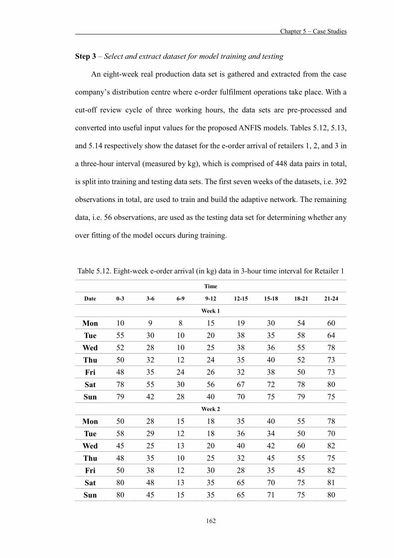
Chapter 5 – Case Studies
162
Step 3 – Select and extract dataset for model training and testing
An eight-week real production data set is gathered and extracted from the case
company’s distribution centre where e-order fulfilment operations take place. With a
cut-off review cycle of three working hours, the data sets are pre-processed and
converted into useful input values for the proposed ANFIS models. Tables 5.12, 5.13,
and 5.14 respectively show the dataset for the e-order arrival of retailers 1, 2, and 3 in
a three-hour interval (measured by kg), which is comprised of 448 data pairs in total,
is split into training and testing data sets. The first seven weeks of the datasets, i.e. 392
observations in total, are used to train and build the adaptive network. The remaining
data, i.e. 56 observations, are used as the testing data set for determining whether any
over fitting of the model occurs during training.
Table 5.12. Eight-week e-order arrival (in kg) data in 3-hour time interval for Retailer 1
Time
Date 0-3 3-6 6-9 9-12 12-15 15-18 18-21 21-24
Week 1
Mon 10 9 8 15 19 30 54 60 Tue 55 30 10 20 38 35 58 64 Wed 52 28 10 25 38 36 55 78 Thu 50 32 12 24 35 40 52 73 Fri 48 35 24 26 32 38 50 73 Sat 78 55 30 56 67 72 78 80 Sun 79 42 28 40 70 75 79 75
Week 2
Mon 50 28 15 18 35 40 55 78 Tue 58 29 12 18 36 34 50 70 Wed 45 25 13 20 40 42 60 82 Thu 48 35 10 25 32 45 55 75 Fri 50 38 12 30 28 35 45 82 Sat 80 48 13 35 65 70 75 81 Sun 80 45 15 35 65 71 75 80

Chapter 5 – Case Studies
163
Week 3 Mon 48 35 14 20 38 38 60 80 Tue 60 32 15 20 40 35 55 74 Wed 50 28 15 23 45 45 58 85 Thu 50 38 14 28 35 48 58 78 Fri 55 40 15 35 30 40 46 85 Sat 82 50 15 38 68 75 80 82 Sun 82 48 16 38 69 74 79 82
Week 4 Mon 50 38 15 22 40 45 58 75 Tue 64 35 18 25 45 38 53 78 Wed 58 30 13 26 50 48 60 85 Thu 50 42 18 30 45 52 60 85 Fri 65 45 18 42 35 45 54 88 Sat 85 55 20 45 72 78 85 85 Sun 85 54 22 42 70 76 82 88
Week 5 Mon 51 32 18 20 32 48 58 75 Tue 60 28 20 25 42 48 55 75 Wed 55 40 22 26 45 47 65 82 Thu 57 45 15 25 35 45 55 75 Fri 50 38 18 30 32 40 48 82 Sat 80 50 28 54 68 80 78 85 Sun 81 48 28 37 68 70 78 81
Week 6 Mon 58 32 18 28 32 48 64 71 Tue 75 45 28 25 48 45 55 75 Wed 65 48 30 28 45 51 69 80 Thu 60 45 20 24 38 45 58 78 Fri 58 41 18 30 32 40 54 82 Sat 80 61 32 51 70 79 84 82 Sun 81 53 32 45 70 75 71 85
Week 7 Mon 50 38 15 22 40 45 58 75 Tue 64 35 18 25 45 38 53 78 Wed 58 30 13 26 50 48 60 85 Thu 50 42 18 30 45 52 60 85
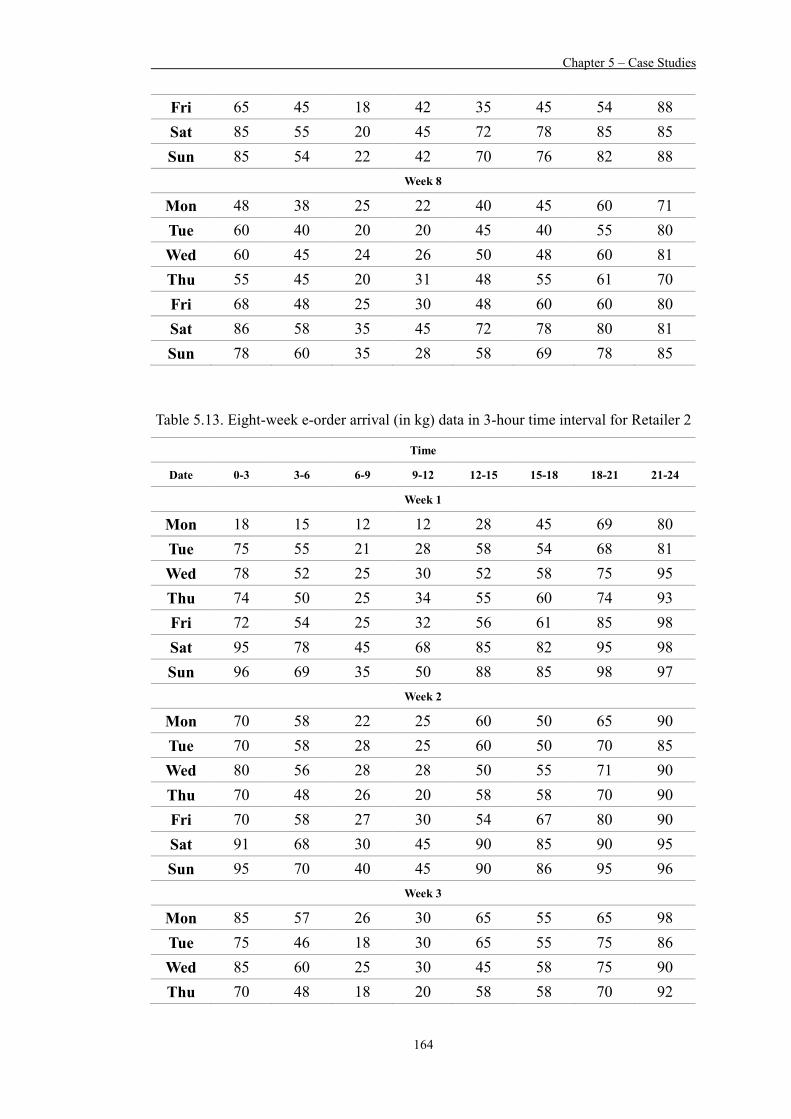
Chapter 5 – Case Studies
164
Fri 65 45 18 42 35 45 54 88 Sat 85 55 20 45 72 78 85 85 Sun 85 54 22 42 70 76 82 88
Week 8 Mon 48 38 25 22 40 45 60 71 Tue 60 40 20 20 45 40 55 80 Wed 60 45 24 26 50 48 60 81 Thu 55 45 20 31 48 55 61 70 Fri 68 48 25 30 48 60 60 80 Sat 86 58 35 45 72 78 80 81 Sun 78 60 35 28 58 69 78 85
Table 5.13. Eight-week e-order arrival (in kg) data in 3-hour time interval for Retailer 2
Time
Date 0-3 3-6 6-9 9-12 12-15 15-18 18-21 21-24
Week 1
Mon 18 15 12 12 28 45 69 80 Tue 75 55 21 28 58 54 68 81 Wed 78 52 25 30 52 58 75 95 Thu 74 50 25 34 55 60 74 93 Fri 72 54 25 32 56 61 85 98 Sat 95 78 45 68 85 82 95 98 Sun 96 69 35 50 88 85 98 97
Week 2
Mon 70 58 22 25 60 50 65 90 Tue 70 58 28 25 60 50 70 85 Wed 80 56 28 28 50 55 71 90 Thu 70 48 26 20 58 58 70 90 Fri 70 58 27 30 54 67 80 90 Sat 91 68 30 45 90 85 90 95 Sun 95 70 40 45 90 86 95 96
Week 3 Mon 85 57 26 30 65 55 65 98 Tue 75 46 18 30 65 55 75 86 Wed 85 60 25 30 45 58 75 90 Thu 70 48 18 20 58 58 70 92

Chapter 5 – Case Studies
165
Fri 80 60 20 35 55 68 82 92 Sat 91 68 20 45 94 88 92 98 Sun 98 72 45 50 91 90 93 94
Week 4 Mon 89 70 18 25 58 89 68 95 Tue 80 58 25 33 68 60 80 90 Wed 92 65 30 40 48 62 80 95 Thu 78 50 22 30 60 65 75 98 Fri 85 65 25 40 60 78 88 96 Sat 96 72 68 54 88 92 90 95 Sun 95 78 48 48 89 95 95 98
Week 5 Mon 75 51 28 30 58 56 70 89 Tue 65 56 32 30 58 68 75 90 Wed 73 55 35 32 53 58 75 91 Thu 75 57 28 20 48 59 75 85 Fri 75 68 30 35 58 70 78 95 Sat 94 71 42 68 91 88 91 94 Sun 98 78 45 69 89 89 95 96
Week 6 Mon 78 58 35 41 58 58 75 85 Tue 78 67 45 38 60 65 78 90 Wed 84 60 45 40 58 61 78 95 Thu 78 60 30 35 54 65 78 90 Fri 71 68 31 38 54 75 80 95 Sat 97 78 45 70 89 89 95 98 Sun 98 80 54 78 85 91 98 98
Week 7 Mon 89 70 18 25 58 89 68 95 Tue 80 58 25 33 68 60 80 90 Wed 92 65 30 40 48 62 80 95 Thu 78 50 22 30 60 65 75 98 Fri 85 65 25 40 60 78 88 96 Sat 96 72 68 54 88 92 90 95 Sun 95 78 48 48 89 95 95 98
Week 8 Mon 80 60 58 25 58 79 71 91
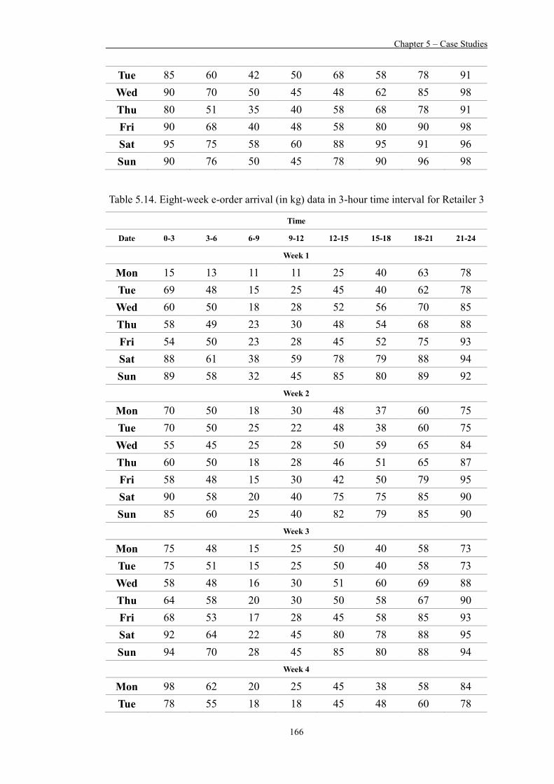
Chapter 5 – Case Studies
166
Tue 85 60 42 50 68 58 78 91 Wed 90 70 50 45 48 62 85 98 Thu 80 51 35 40 58 68 78 91 Fri 90 68 40 48 58 80 90 98 Sat 95 75 58 60 88 95 91 96 Sun 90 76 50 45 78 90 96 98
Table 5.14. Eight-week e-order arrival (in kg) data in 3-hour time interval for Retailer 3
Time
Date 0-3 3-6 6-9 9-12 12-15 15-18 18-21 21-24
Week 1
Mon 15 13 11 11 25 40 63 78 Tue 69 48 15 25 45 40 62 78 Wed 60 50 18 28 52 56 70 85 Thu 58 49 23 30 48 54 68 88 Fri 54 50 23 28 45 52 75 93 Sat 88 61 38 59 78 79 88 94 Sun 89 58 32 45 85 80 89 92
Week 2
Mon 70 50 18 30 48 37 60 75 Tue 70 50 25 22 48 38 60 75 Wed 55 45 25 28 50 59 65 84 Thu 60 50 18 28 46 51 65 87 Fri 58 48 15 30 42 50 79 95 Sat 90 58 20 40 75 75 85 90 Sun 85 60 25 40 82 79 85 90
Week 3 Mon 75 48 15 25 50 40 58 73 Tue 75 51 15 25 50 40 58 73 Wed 58 48 16 30 51 60 69 88 Thu 64 58 20 30 50 58 67 90 Fri 68 53 17 28 45 58 85 93 Sat 92 64 22 45 80 78 88 95 Sun 94 70 28 45 85 80 88 94
Week 4 Mon 98 62 20 25 45 38 58 84 Tue 78 55 18 18 45 48 60 78

Chapter 5 – Case Studies
167
Wed 64 50 20 28 55 58 65 85 Thu 79 64 22 35 48 64 60 85 Fri 78 60 25 32 48 65 90 95 Sat 89 69 25 48 88 85 81 90 Sun 89 75 35 48 88 85 90 91
Week 5 Mon 68 48 22 35 50 40 58 78 Tue 69 48 30 28 45 50 65 85 Wed 74 54 30 28 54 61 70 86 Thu 69 50 25 28 41 51 68 87 Fri 65 54 22 32 48 68 68 90 Sat 88 67 32 58 78 79 88 91 Sun 86 68 30 50 78 80 88 89
Week 6 Mon 69 51 25 35 50 53 68 75 Tue 71 54 38 35 54 51 65 85 Wed 75 55 35 35 54 58 75 85 Thu 70 54 28 29 45 58 70 85 Fri 64 61 22 32 48 68 72 88 Sat 90 71 38 60 75 85 90 90 Sun 88 78 48 70 80 84 80 90
Week 7 Mon 98 62 20 25 45 38 58 84 Tue 78 55 18 18 45 48 60 78 Wed 64 50 20 28 55 58 65 85 Thu 79 64 22 35 48 64 60 85 Fri 78 60 25 32 48 65 90 95 Sat 89 69 25 48 88 85 81 90 Sun 89 75 35 48 88 85 90 91
Week 8 Mon 71 56 40 25 45 70 62 82 Tue 75 51 31 25 45 50 68 80 Wed 65 51 30 35 55 58 70 89 Thu 75 61 25 38 55 61 65 81 Fri 80 61 35 45 50 70 85 91 Sat 90 65 45 48 80 90 85 89 Sun 85 70 45 35 65 88 89 90
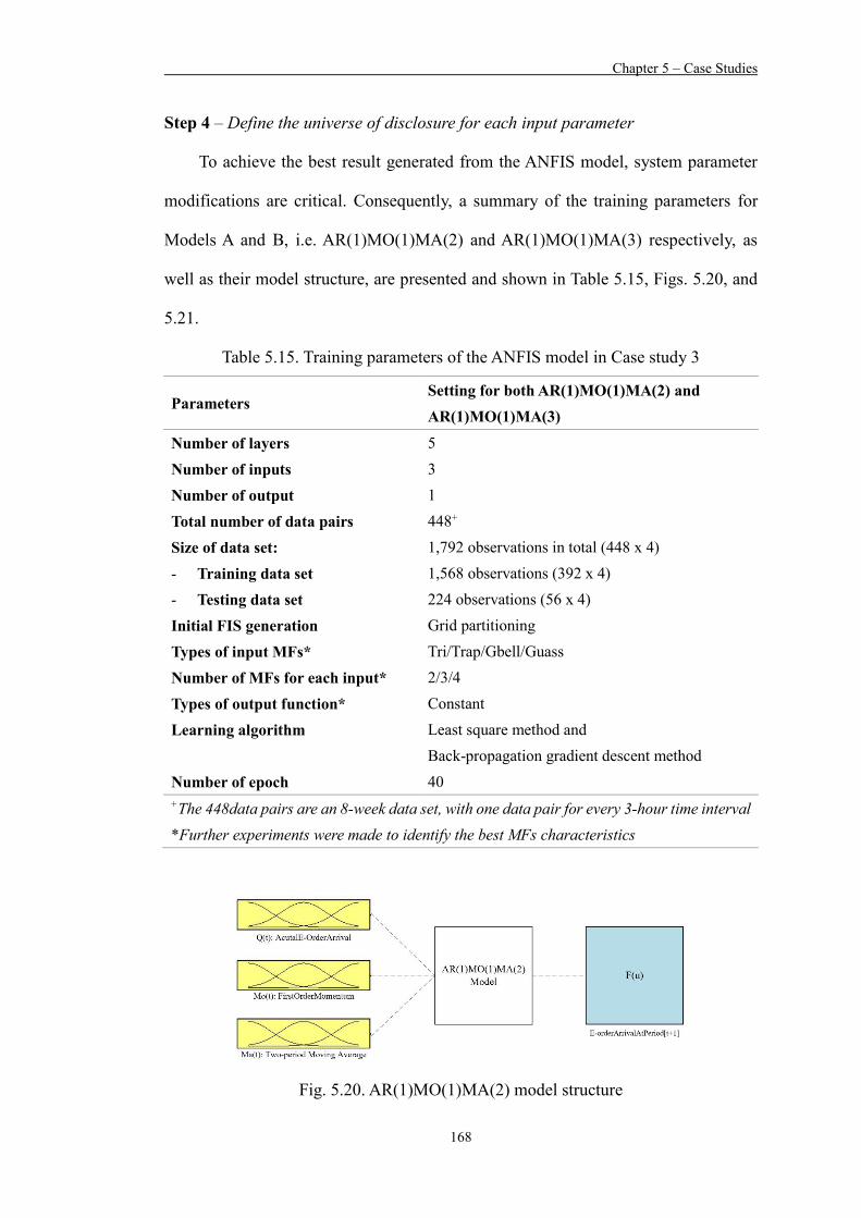
Chapter 5 – Case Studies
168
Step 4 – Define the universe of disclosure for each input parameter
To achieve the best result generated from the ANFIS model, system parameter
modifications are critical. Consequently, a summary of the training parameters for
Models A and B, i.e. AR(1)MO(1)MA(2) and AR(1)MO(1)MA(3) respectively, as
well as their model structure, are presented and shown in Table 5.15, Figs. 5.20, and
5.21.
Table 5.15. Training parameters of the ANFIS model in Case study 3
Parameters Setting for both AR(1)MO(1)MA(2) and AR(1)MO(1)MA(3)
Number of layers 5 Number of inputs 3 Number of output 1 Total number of data pairs 448+ Size of data set: 1,792 observations in total (448 x 4) - Training data set 1,568 observations (392 x 4) - Testing data set 224 observations (56 x 4) Initial FIS generation Grid partitioning Types of input MFs* Tri/Trap/Gbell/Guass Number of MFs for each input* 2/3/4 Types of output function* Constant Learning algorithm Least square method and
Back-propagation gradient descent method Number of epoch 40 +The 448data pairs are an 8-week data set, with one data pair for every 3-hour time interval *Further experiments were made to identify the best MFs characteristics
Fig. 5.20. AR(1)MO(1)MA(2) model structure
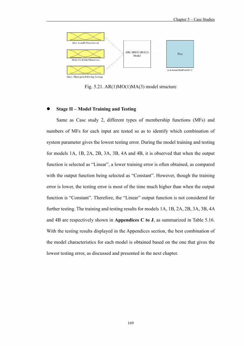
Chapter 5 – Case Studies
169
Fig. 5.21. AR(1)MO(1)MA(3) model structure
Stage II – Model Training and Testing
Same as Case study 2, different types of membership functions (MFs) and
numbers of MFs for each input are tested so as to identify which combination of
system parameter gives the lowest testing error. During the model training and testing
for models 1A, 1B, 2A, 2B, 3A, 3B, 4A and 4B, it is observed that when the output
function is selected as “Linear”, a lower training error is often obtained, as compared
with the output function being selected as “Constant”. However, though the training
error is lower, the testing error is most of the time much higher than when the output
function is “Constant”. Therefore, the “Linear” output function is not considered for
further testing. The training and testing results for models 1A, 1B, 2A, 2B, 3A, 3B, 4A
and 4B are respectively shown in Appendices C to J, as summarized in Table 5.16.
With the testing results displayed in the Appendices section, the best combination of
the model characteristics for each model is obtained based on the one that gives the
lowest testing error, as discussed and presented in the next chapter.

Chapter 5 – Case Studies
170
Table 5.16. A summary of the ANFIS model training and testing results
Typology Retailer Model Appendix
II
1 1A C 1B D
2 2A E 2B F
3 3A G 3B H
I Aggregated e-order
arrival of retailer 1, 2 and 3
4A I 4B J
Stage III – Performance Evaluations
To evaluate the feasibility of the developed ANFIS model for forecasting the e-
order arrival, the same as in Case study 2, with the best model setting identified for
each model (Models 1A, 1B, 2A, 2B, 3A, 3B, 4A and 4B) in Stage II, these developed
ANFIS models are then compared with an autoregressive integrated moving average
(ARIMA) model for further performance validation. However, as two different
typologies are introduced in this case study, performance evaluations are not
undertaken to compare the ANFIS model and the ARIMA model only. Instead,
performance evaluation consists of four major comparisons. A model comparison
framework, as shown in Fig. 5.22, is constructed to better illustrate the performance
evaluation process adopted. The four prediction performance comparisons are:
(i) Comparison 1 – Model A vs Model B: Model A and B comparison for each
individual retailer’s ANFIS model
(ii) Comparison 2 – Typology 1 vs Typology 2 for ANFIS model: ANFIS model
prediction performance comparison between typologies 1 and 2
(iii) Comparison 3 – Typology 1 vs Typology 2 for ARIMA model: ARIMA
model prediction performance comparison between typologies 1 and 2
Chapter 5 – Case Studies
171
(iv) Comparison 4 (the ultimate comparison) – ANFIS vs ARIMA: Prediction
performance comparison between the best ANFIS model and the best ARIMA
model.
5.5 Summary
In this chapter, three case studies are presented. The three modules of the EF-
DSS are separately deployed for different logistics service providers according to their
existing operational bottlenecks and needs. The ECM and EGM are applied in Case
study 1, whereas the ECM and EBRM are applied in Case Studies 2 and 3. As the
implementation of the EF-DSS in Case studies 2 and 3 are different in terms of: (i) the
methodologies adopted for ANFIS model construction, (ii) the dataset used for model
training and testing, and (iii) the set of input variables introduced in the ANFIS models
for order arrival prediction, the results upon the implementation of EF-DSS in Case
study 2 and 3 are discussed and compared in the next chapter. Furthermore, with the
EF-DSS deployed in three different case companies, the performance of the EF-DSS,
as well as the operating performance of each case company upon the system
implementation, are thoroughly discussed in the next chapter.

Chapter 5 – Case Studies
172
Fig. 5.22. Model performance comparison framework

Chapter 6 – Results and Discussion
173
Chapter 6 – Results and Discussion
6.1 Introduction
In this research, the Warehouse Postponement Strategy is proposed to streamline
the e-fulfillment operations of e-commerce order handling in distribution centres. To
deploy the proposed operational strategy, two critical decisions, i.e. How to group e-
orders, and when to release the grouped orders, need to be made manually by the
logistics service providers. Therefore, the EF-DSS is proposed and developed in this
research to support the logistics service providers in implementing WPS with the
relevant decision support. EF-DSS adopts the GA technique, rule-based inference
engine, autoregressive models and ANFIS models to group the e-orders based on their
similarity of storage locations, and identify the optimal cut-off time for releasing the
grouped e-orders. In this chapter, the results and discussion of the research is presented
in two areas: (i) Experimental results and discussion of the system based on the three
case studies, and (ii) Research, managerial, and practical implications.
6.2 Experimental Results and Discussion of the System
Three case studies are conducted to implement the EF-DSS, which consists of
the E-order Consolidation Module (ECM), E-order Grouping Module (EGM) and E-
order Batch Releasing Module (EBRM). The first case study implemented the ECM
and EGM of the EF-DSS for solving the problem of order grouping. The second and
the third case study implemented the ECM and EBRM of the EF-DSS for identifying
the timing for releasing the grouped orders for performing e-order fulfilment
operations in a batch. In this section, the experimental results and discussion of the
system in the three case studies are presented separately.

Chapter 6 – Results and Discussion
174
6.2.1 Results and Discussion of the GA Parameter Settings in the EGM from
Case Study 1
The e-fulfilment process in warehouses or distribution centers is re-engineered.
Logistics service providers no longer perform e-order fulfilment operations
immediately after orders are received online. Instead, e-orders, which are placed by
B2C customers from various online sales platforms, and usually small in lot-size, are
consolidated in a cloud database for further order grouping. In addition to the order
grouping decision support by separating pending to-be-picked SKUs into several order
grouping lists based on storage locations dissimilarity, the operating procedures and
appropriate material handling equipment are further suggested for ease of e-order
fulfilment process execution. The improvement is not only beneficial to the case
company, but also its downstream logistics service providers along the supply chain.
In this section, the GA optimal parameter setting is first reported, followed by an
analysis of the key performance improvement areas found in the case company.
(i) Parameter settings of the Genetic Algorithm
The GA parameter settings are required to be defined prior to implementation in
an actual production environment. Specifically, the crossover rate and mutation rate,
ranging from 0 to 1, are defined by the users. A trial-and-error approach is used to
determine an appropriate crossover and mutation rates that best suit the GA
mechanism developed. In Case Study 1, a crossover rate of 0.7 and 0.9, and a mutation
rate of 0.1 and 0.25, are selected for testing in a population size of 2000 and with the
number of generations set as 50,000. Using different combinations of the crossover
and mutation rate, as specified in Table 6.1, it is found that, after pair-wise executing
10 times, a GA parameter setting with a crossover rate of 0.9 and a mutation rate of
0.1 gives the lowest fitness value, as summarized and shown in Fig. 6.1. The more

Chapter 6 – Results and Discussion
175
storage locations to be visited, a greater number of trials is preferred, so as to obtain a
better nearly-optimal solution.
Fig. 6.1. Graphical comparison of the results under different combinations of GA
parameter setting
Table 6.1. Optimal parameter settings for the Genetic Algorithm
Parameter Settings Crossover rate 0.7/0.9 Mutation rate 0.1/0.25 Population size 2000
Termination criteria
Stops if: (1) the number of generations reach 50,000; or (2) the target cell has an improvement of less than
0.01% in the last 10,000 trials.

Chapter 6 – Results and Discussion
176
(ii) Key operating performance improvements
The performance improvement in the order fulfilment operations in the e-
fulfilment centres of Case Study 1 can be found in terms of two measurable areas,
namely: Reduction of total order processing time, and reduction of total traveling
distance of a customer order.
Reduction of total order processing time
The total order processing time in handling an e-order in e-fulfillment centers
involves the following sequential operations:
I. Order planning – Consolidate e-orders and print relevant documents for
warehouse operators to execute accordingly;
II. Order picking – Travel to storage locations and pick the required items;
III. Order packing and consolidation – Allocate the picked items to the designated
customer order and pack the items in a carton box; and
IV. Labeling – Print and stick the required label(s) on the packed carton box.
Before the implementation of EF-DSS, e-orders were processed individually
without any grouping of orders in advance for future batch processing. Therefore, the
order processing operation did not consist of any order planning operation that
consolidated e-orders before process execution. E-orders are immediately picked by
assigning a worker to travel to the specified storage locations to pick up the required
items. After the picked items are inspected, the items are loaded into a carton box at
the packing area, followed by placing the shipping and precaution labels on the packed
carton box. According to previous time measurement conducted by the case company,
the total e-order processing time of an order, involving the operations mentioned above,
was 9.33 minutes on average, as shown in Table 6.2.
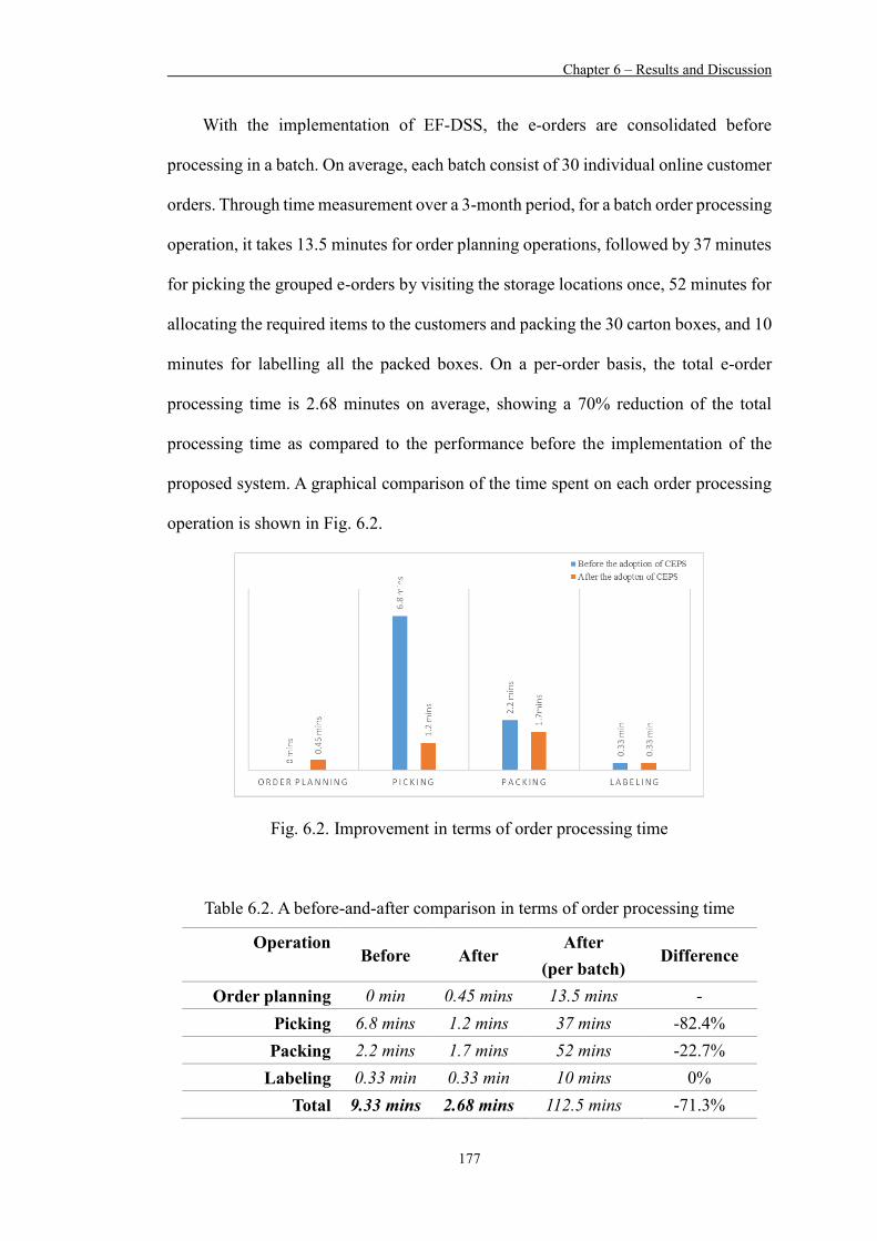
Chapter 6 – Results and Discussion
177
With the implementation of EF-DSS, the e-orders are consolidated before
processing in a batch. On average, each batch consist of 30 individual online customer
orders. Through time measurement over a 3-month period, for a batch order processing
operation, it takes 13.5 minutes for order planning operations, followed by 37 minutes
for picking the grouped e-orders by visiting the storage locations once, 52 minutes for
allocating the required items to the customers and packing the 30 carton boxes, and 10
minutes for labelling all the packed boxes. On a per-order basis, the total e-order
processing time is 2.68 minutes on average, showing a 70% reduction of the total
processing time as compared to the performance before the implementation of the
proposed system. A graphical comparison of the time spent on each order processing
operation is shown in Fig. 6.2.
Fig. 6.2. Improvement in terms of order processing time
Table 6.2. A before-and-after comparison in terms of order processing time
Operation Before After
After (per batch)
Difference
Order planning 0 min 0.45 mins 13.5 mins - Picking 6.8 mins 1.2 mins 37 mins -82.4% Packing 2.2 mins 1.7 mins 52 mins -22.7%
Labeling 0.33 min 0.33 min 10 mins 0% Total 9.33 mins 2.68 mins 112.5 mins -71.3%
Chapter 6 – Results and Discussion
178
Reduction of total traveling distance of a customer order
The total travelling distance is another noticeable improvement area. The
adoption of EF-DSS has reduced the traveling distance of an e-order, as storage
locations are visited only once for a batch of consolidated customer orders, instead of
conventionally visiting storage locations repeatedly throughout the working hours for
each particular customer order. Before the re-engineered order fulfilment operations,
the items purchased in an e-commerce order were picked by visiting the storage
locations once, which, on average, required a travel distance of 68 meters. With the
implementation of EF-DSS, a batch, which consists of 30 individual online customer
orders on average, requires a total travel distance of 397 meters. In other words, a
travel distance of only 13.2 meters is required for an order, yielding a 81% reduction
of total traveling distance in handling a customer order. In the long run, the re-
engineered e-order process reduces the workload of employees working in e-
fulfilment operations. The saved time for repeated visits to storage locations enables
managers to flexibly reallocate the human resources to handle other operations, such
as put-away and cargo loading or unloading operations.
6.2.2 Results and Discussion of the AR-MO-ANFIS Model Parameter Settings
in the EBRM from Caste Study 2
In Case Study 2, two ANFIS-based models, AR(1)MO(1) and AR(1)MO(2)
model, are developed for forecasting the arrival frequency of e-commerce orders in
the case company’s distribution centres. The output of the ANFIS-based models, i.e.
the predicted volume of e-commerce order arrival (in terms of kg) for the upcoming
two-hour period in the distribution centres, serves as one of the inputs of another
proposed algorithm in the EBRM of the EF-DSS, so as to identify the optimal cut-off
time for releasing the grouped orders that are currently consolidated in the E-order
Chapter 6 – Results and Discussion
179
consolidation pool of the ECM of the EF-DSS, and pending for batch release to the
distribution centres for actual process execution. As the prediction ability of the two
developed ANFIS-based models have a significant effect on identifying the final
output of EBRM, i.e. the optimal cut-off time of releasing the grouped orders, model
evaluation and comparison must be performed.
In this section, the ANFIS model comparison and evaluations are first reported.
The performance of the ANFIS models are compared in two separate stages. First,
various combination settings for the AR(1)MO(1) and AR(1)MO(2) models are tested,
so as to obtain the best setting that gives the highest prediction accuracy. Second, the
optimized setting of the AR(1)MO(1) and AR(1)MO(2) models is further compared
with ARIMA model to evaluate the performance of the ANFIS model in the prediction
of e-order arrival. Evaluation of the performance of the ANFIS models in the first stage
and second stage is discussed in (i) Performance comparison of the ANFIS system
parameters and (ii) Performance comparison of the developed ANFIS and ARIMA
models respectively. Lastly, an analysis of the key performance improvement areas
found in the case company is presented in (iii) Order handling performance
comparison.
(i) Performance comparison of the ANFIS system parameters
Various settings, regarding the types of MFs, the number of MFs, and the types
of output function, are evaluated for the two proposed ANFIS models, the AR(1)MO(1)
and AR(1)MO(2) models. The best combination of settings for the AR(1)MO(1) and
AR(1)MO(2) models, as depicted in Table 6.3, is obtained through a comprehensive
evaluation and error analysis for each of the models, as shown in the Appendices A
and B. One of the noticeable issues during the evaluation of the models is the problem
of model over fitting during training. In the Appendices A and B, especially for the

Chapter 6 – Results and Discussion
180
AR(1)MO(2) model, it is found that a lower training error is often obtained when the
output function is set as linear, and when the number of membership functions is larger.
However, the testing error of these settings (for example, the number of MFs for each
input is four, in Gbell-shape, and the output function is set as linear) is very large.
These are perfect examples where the model over fits the training data. To avoid the
model from over fitting, we determine the best combination of settings based on the
one that gives the lowest testing error. The corresponding ANFIS information for both
models under the best structure is respectively shown in Table 6.3, which confirms
that the total number of parameters in the network is fewer than the number of training
data pairs. With the best combination of the setting obtained for AR(1)MO(1) and
AR(1)MO(2), their network structure and test results are respectively shown in Figs.
6.3 to 6.6. Then, error analysis is performed for evaluating and comparing the
prediction performance of these models under their corresponding best setting with
the ARIMA model.
Table 6.3. The characteristics of the best structure of AR(1)MO(1) and AR(1)MO(2)
model and their corresponding ANFIS information
Characteristics of the best structure of the ANFIS for: AR(1)MO(1) AR(1)MO(2) Number of MFs for each input 4, 4 2, 4, 3 Types of input MFs Guass Gbell Types of output function Constant Constant The corresponding ANFIS information Number of nodes 53 72 Number of linear parameters 16 24 Number of nonlinear parameters 16 27 Total number of parameters 32 51 Number of training data pairs 302 302 Number of checking data pairs 34 34 Number of fuzzy rules 16 24
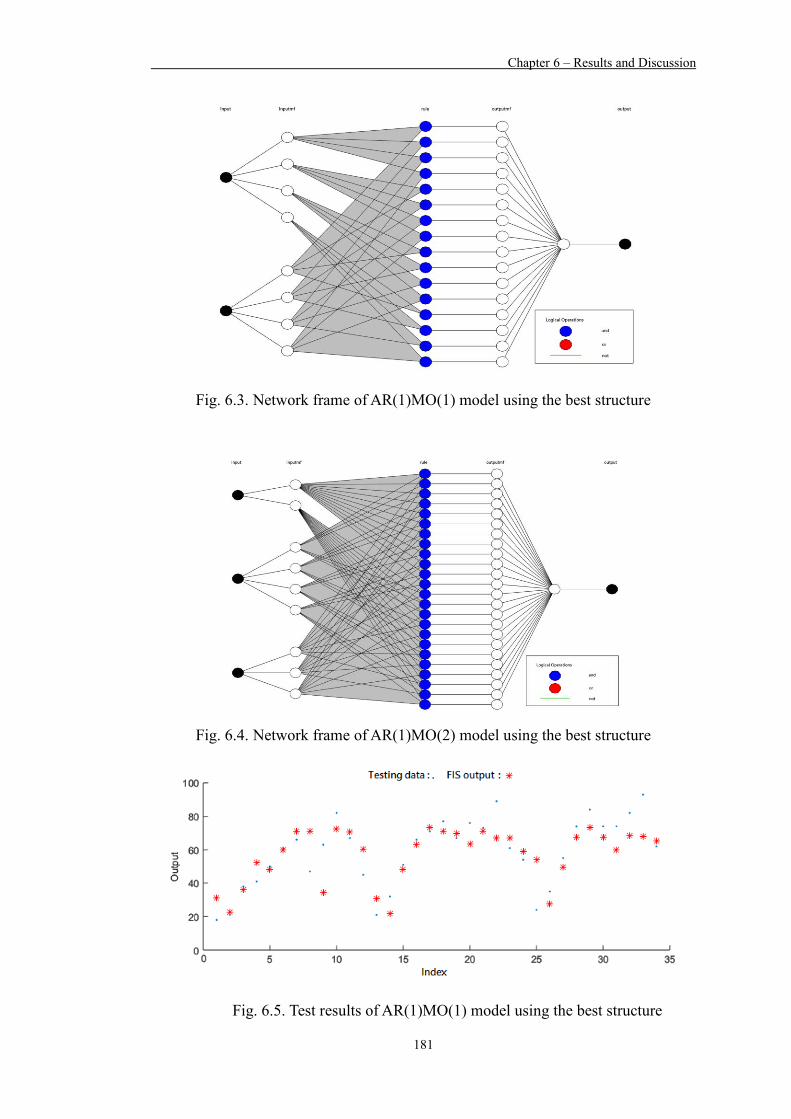
Chapter 6 – Results and Discussion
181
Fig. 6.3. Network frame of AR(1)MO(1) model using the best structure
Fig. 6.4. Network frame of AR(1)MO(2) model using the best structure
Fig. 6.5. Test results of AR(1)MO(1) model using the best structure

Chapter 6 – Results and Discussion
182
Fig. 6.6. Test results of AR(1)MO(2) model using the best structure
(ii) Performance comparison of the developed ANFIS and ARIMA models
The AR(1)MO(1) and AR(1)MO(2) models are compared with the ARIMA
model to evaluate the predicting ability of the developed ANFIS models. The same
four-week data set, which is used for training and testing the AR(1)MO(1) and
AR(1)MO(2) models, is also used for building the ARIMA(p,q)(r,s) model. By
selecting the maximum number of the autoregressive (AR), moving average (MA),
seasonal autoregressive (SAR) and seasonal moving average (SMA) terms, say p, q, r,
s, of the ARIMA model, as well as the periodicity of the seasonal terms using thte
EViews software package, an ARIMA(3,2)(1,1) model, which obtains the lowest
Akaike information criterion (AIC) value, is selected after generating 100 ARMA
models, as shown in Figs. 6.7 and 6.8. Then, another one-week historical data set,
consisting of a total of 84 e-order arrival figures in a two-hour interval, is used for
comparison of the AR(1)MO(1), AR(1)MO(2), and ARIMA(3,2)(1,1) models. Table
6.4 shows the test results of the three models with respect to RMSE, MAD, and MAPE,
as introduced in section 3.6.2.3. Figs. 6.9 and 6.10 show a comparison of the actual
and predicted e-order arrival figures using the AR(1)MO(1), AR(1)MO(2) and
ARIMA(3,2)(1,1) models for the 84 observations. It is shown that both AR(1)MO(1)
and AR(1)MO(2) outperform ARIMA in predicting the e-order arrival. In addition to

Chapter 6 – Results and Discussion
183
these error measures, the accuracy of each prediction value is also considered. The
case company management suggests that a predicted e-order arrival with ±10kg error
is generally acceptable. Thus, by counting the number of accurate items (the difference
between predicted value and actual value being less than 10) in the 84 observations,
the item accuracy of AR(1)MO(1) and AR(1)MO(2) achieves levels of 85.7% and
86.9% respectively, which is better than that of ARIMA model (79.8%), as depicted in
Table 6.5. This further confirms the satisfactory predicting ability of the proposed
ANFIS models.
Fig. 6.7. Automatic ARIMA model selection result for case study 1
Fig. 6.8. Forecast comparison graph showing the selected model (in red) and other
ARIMA models (in grey) for case study 1

Chapter 6 – Results and Discussion
184
Table 6.4. Error analysis for model comparison for case study 1
Model comparison Error measures: AR(1)MO(1) AR(1)MO(2) ARIMA
RMSE 6.79 7.40 9.56 MAD 4.66 5.20 6.54
MAPE (%) 10.65% 11.79% 14.79%
Table 6.5. Item accuracy comparison for case study 1
Model comparison AR(1)MO(1) AR(1)MO(2) ARIMA
No. of accurate items 72 73 67 No. of inaccurate items 12 11 17 Total number of items 84 84 84
Item accuracy 85.7% 86.9% 79.8%
Fig. 6.9. Comparison of actual and predicted e-order arrival using AR(1)MO(1),
AR(1)MO(2) and ARIMA model for observation no. 1-42

Chapter 6 – Results and Discussion
185
Fig. 6.10. Comparison of actual and predicted e-order arrival using AR(1)MO(1),
AR(1)MO(2) and ARIMA model for observation no. 43-84
(iii) Order handling performance comparison
The deployment of EF-DSS, integrating the AR(1)MO(2) ANFIS models,
improves the order handling performance in terms of the order handling efficiency and
resource management, which are respectively measured by the number of e-orders
processed within a designated period, and the traveling distance per worker. The
results of a before-and-after comparison of the e-order handling performance in the e-
fulfilment centres is shown in Table 6.6. Before the introduction of EF-DSS, e-orders
were processed individually upon receiving notification from the retailers. The number
of processed orders within a half working day is, on average, 362 orders. After the
implementation of EF-DSS, the average number of processed orders within a half
working day is 569 orders, a 57% improvement of the order handling efficiency.
Besides, better resource management is achieved as the traveling distance per worker
per working day is reduced from 978 meters to 467 meters, a 52% reduction. The
number of visits to the storage area per day for a worker is also reduced from 16 times
to only 5 times. The reduction of traveling distance is credited to the re-engineered

Chapter 6 – Results and Discussion
186
flow of e-order handling, in which an e-order is no longer picked from its storage
location immediately upon being received from the retailer, but is consolidated in the
e-order consolidation pool of the EF-DSS for batch release and picking. Therefore, the
total traveling distance and the number of visits to storage locations per day have been
drastically reduced.
Table 6.6. A before-and-after comparison of e-order handling and resource
management
Order handling and resource allocation improvement
Without EAPS
With EAPS
% of improvement
No. of processed orders (per 0.5 working day)
362 orders 569 orders 57%
Traveling distance per worker (per working day)
978 meters 467 meters 52%
No. of visits to the storage area per worker (per working day)
16 times 5 times 69%
6.2.3 Results and Discussion of the AR-MO-MA-ANFIS Model Parameter
Settings in the EBRM from Case Study 3
In Case Study 3, a total of 8 ANFIS-based models are developed under two
typologies, as summarized in Table 6.7, for forecasting the arrival frequency of e-
commerce orders in the case company’s distribution centres. The output of the ANFIS-
based models, i.e. the predicted volume of e-commerce order arrivals (in terms of kg)
for the upcoming three-hour period in the distribution centres, serves as one of the
inputs of another algorithm in the EBRM of the EF-DSS, so as to identify the optimal
cut-off time for releasing the grouped orders that are currently consolidated in the E-
order consolidation pool of the ECM of the EF-DSS, and pending for batch release to
the distribution centres for actual process execution.

Chapter 6 – Results and Discussion
187
Table 6.7. A summary of the ANFIS models developed in Case study 3
Typology Retailer Model Set of input variables
II
1 1A AR(1), MO(1), MA(2) 1B AR(1), MO(1), MA(3)
2 2A AR(1), MO(1), MA(2) 2B AR(1), MO(1), MA(3)
3 3A AR(1), MO(1), MA(2) 3B AR(1), MO(1), MA(3)
I Aggregated e-order arrival
of retailer 1, 2 and 3 4A AR(1), MO(1), MA(2) 4B AR(1), MO(1), MA(3)
As discussed in the previous chapter, a model performance comparison
framework, which consists of 4 comparisons, is formulated for systematically
evaluating the prediction ability of each model and typology. This section provides
error analysis of each model for making model comparisons, thereby providing
implications through each comparison. In total, 10 findings are generated using the
model performance comparison framework presented in Fig. 5.22.
(i) Comparison 1 – Model A vs Model B: Model A and B comparison for each
individual retailer’s ANFIS model
Through the model training and testing processes for each model developed in
Case study 3, the performance of each model under different combinations of model
setting is identified and presented in Appendices C to J, where the best model setting
is one that gives the minimum testing error. A summary of the best model setting for
each model, i.e. Models 1A, 1B, 2A, 2B, 3A, 3B, 4A, and 4B, is shown in Table 6.8.
Using the corresponding training dataset for each retailer, each model is then tested
with the testing dataset. The test results of the best models for each retailer’s dataset

Chapter 6 – Results and Discussion
188
and for the dataset aggregating all retailers are respectively depicted in Figs. 6.11 to
6.14. Several findings can be obtained from observing Table 6.8, they are:
Finding 1 (Output function) – “Constant” output function is far better than
the “Linear” funcation: When the training error is very low and the testing error
extremely high, the model is said to be overfitting with the training data. That
means the model is a good forecasting model. In performing model training and
testing in this case study, overfitting training dataset is an obvious problem found
in models with “Linear” output function. This finding is consistent with the
model training and testing results in Case study 2 in which, the problem of
overfitting with training dataset also exists when the output function is set as
“Linear”. Therefore, setting the output function as “Constant” when deploying
the EF-DSS is more appropriate.
Finding 2 (Types of MFs) – No specific type of membership function gives a
better predicting performance: Triangle (Tri), trapezoid (Trap), Gbell, and
Guass membership functions have been used for model training and testing. The
results, as shown in Table 6.8, indicate that there is no specific type of
membership function that outperforms the others. In this regard, different types
of MFs should be tested during the model training and testing process.
Finding 3 (No. of MFs) – Input with two membership functions generally gives
better predicting performance: During the model training and testing process,
the number of MFs for an input variable is set as either 2, 3, or 4. MFs higher
than 4 would hugely increase the computation time, require stronger
computation power, and require a larger training dataset. Results shown in Table
6.8 reveal that the majority of the time, the best model can be obtained with
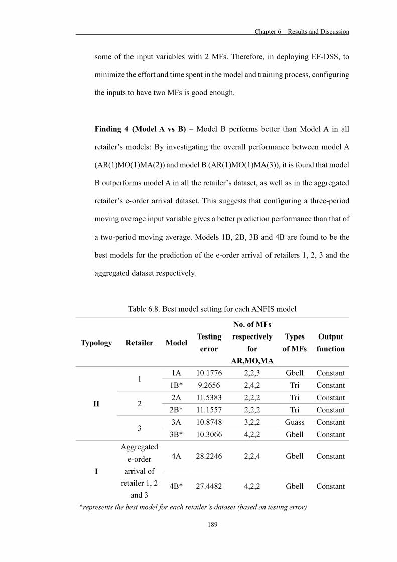
Chapter 6 – Results and Discussion
189
some of the input variables with 2 MFs. Therefore, in deploying EF-DSS, to
minimize the effort and time spent in the model and training process, configuring
the inputs to have two MFs is good enough.
Finding 4 (Model A vs B) – Model B performs better than Model A in all
retailer’s models: By investigating the overall performance between model A
(AR(1)MO(1)MA(2)) and model B (AR(1)MO(1)MA(3)), it is found that model
B outperforms model A in all the retailer’s dataset, as well as in the aggregated
retailer’s e-order arrival dataset. This suggests that configuring a three-period
moving average input variable gives a better prediction performance than that of
a two-period moving average. Models 1B, 2B, 3B and 4B are found to be the
best models for the prediction of the e-order arrival of retailers 1, 2, 3 and the
aggregated dataset respectively.
Table 6.8. Best model setting for each ANFIS model
Typology Retailer Model Testing error
No. of MFs respectively
for AR,MO,MA
Types of MFs
Output function
II
1 1A 10.1776 2,2,3 Gbell Constant 1B* 9.2656 2,4,2 Tri Constant
2 2A 11.5383 2,2,2 Tri Constant 2B* 11.1557 2,2,2 Tri Constant
3 3A 10.8748 3,2,2 Guass Constant 3B* 10.3066 4,2,2 Gbell Constant
I
Aggregated e-order
arrival of retailer 1, 2
and 3
4A 28.2246 2,2,4 Gbell Constant
4B* 27.4482 4,2,2 Gbell Constant
*represents the best model for each retailer’s dataset (based on testing error)
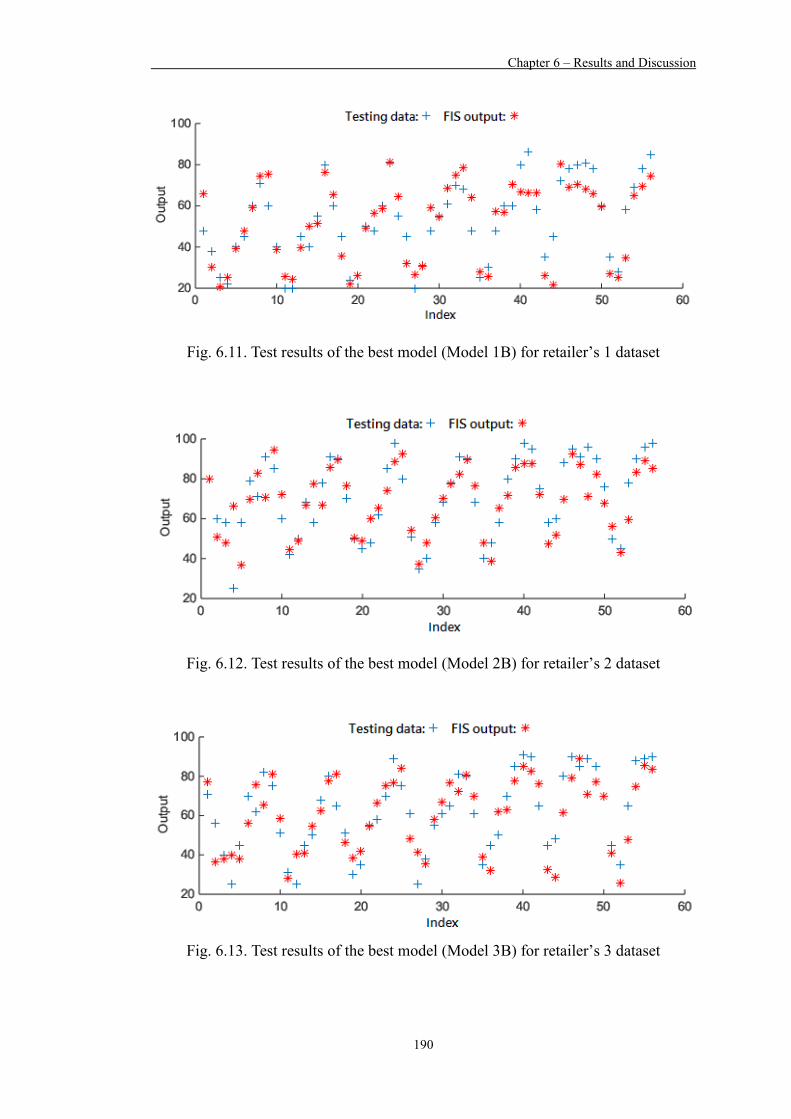
Chapter 6 – Results and Discussion
190
Fig. 6.11. Test results of the best model (Model 1B) for retailer’s 1 dataset
Fig. 6.12. Test results of the best model (Model 2B) for retailer’s 2 dataset
Fig. 6.13. Test results of the best model (Model 3B) for retailer’s 3 dataset

Chapter 6 – Results and Discussion
191
Fig. 6.14. Test results of the best model (Model 4B) for the dataset aggregating
retailers 1, 2 and 3
(ii) Comparison 2 – Typology 1 vs Typology 2 for ANFIS model: ANFIS model
prediction performance comparison between typology 1 and 2
With the best model setting determined for each model, the prediction
performance of models A and B under each retailer’s dataset and the aggregated
dataset is compared. Based on the training error (the lower the better), the best model
for each retailer’s dataset is identified as summarized in Table 6.8. In this comparison,
to compare the prediction performance between typology I (aggregating all
retailers for the prediction) and II (Separately predicting each individual retailer),
another set of real data, which consists of one-week e-order arrivals in a three-
hour horizon, is gathered in the distribution centre of the case company. The best
model for retailers 1, 2, and 3, as well as for the aggregated dataset, i.e. Models 1B,
2B, 3B and 4B respectively, are used to predict a one-week actual e-order arrivals data.
The one-week of data for each retailer for performance evaluations of Models 1B, 2B,
3B is respectively shown in Tables 6.9 to 6.11. By summing up the one-week data of
each retailer, an aggregated dataset for all retailers is formulated as shown in Table
6.12, for performance evaluation of Model 4B.

Chapter 6 – Results and Discussion
192
Table 6.9. Another one-week e-order arrival dataset for Retailer 1
Time
Date 0-3 3-6 6-9 9-12 12-15 15-18 18-21 21-24
Week 1
Mon 62 33 20 26 45 52 68 79 Tue 69 41 25 17 37 49 61 77 Wed 65 38 19 30 59 70 74 81 Thu 63 37 21 31 55 64 73 79 Fri 68 41 30 32 55 66 74 81 Sat 64 35 28 39 56 68 79 84 Sun 65 31 30 46 64 70 79 77
Table 6.10. Another one-week e-order arrival dataset for Retailer 2
Time
Date 0-3 3-6 6-9 9-12 12-15 15-18 18-21 21-24
Week 1
Mon 77 55 29 38 52 69 81 92 Tue 76 57 41 43 66 79 94 96 Wed 83 52 28 45 60 79 88 90 Thu 75 50 29 45 67 79 93 95 Fri 83 50 37 56 73 78 89 95 Sat 97 72 43 44 65 78 89 92 Sun 89 79 49 38 48 65 83 90
Table 6.11. Another one-week e-order arrival dataset for Retailer 3
Time
Date 0-3 3-6 6-9 9-12 12-15 15-18 18-21 21-24
Week 1
Mon 77 52 27 44 57 77 81 83 Tue 68 48 32 46 56 77 83 89 Wed 72 51 24 36 55 74 84 90 Thu 70 45 25 41 62 78 83 91 Fri 79 48 18 33 56 65 77 82 Sat 72 61 40 38 57 70 83 89 Sun 80 61 38 29 51 66 79 87
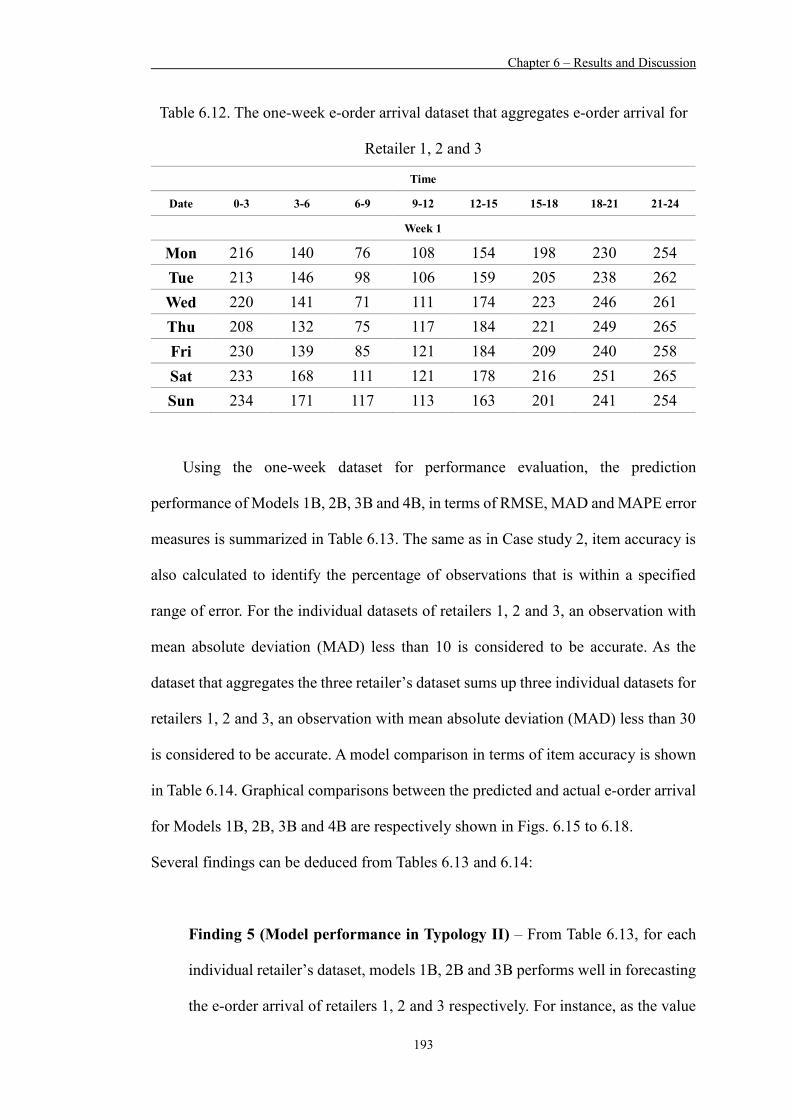
Chapter 6 – Results and Discussion
193
Table 6.12. The one-week e-order arrival dataset that aggregates e-order arrival for
Retailer 1, 2 and 3
Time
Date 0-3 3-6 6-9 9-12 12-15 15-18 18-21 21-24
Week 1
Mon 216 140 76 108 154 198 230 254 Tue 213 146 98 106 159 205 238 262 Wed 220 141 71 111 174 223 246 261 Thu 208 132 75 117 184 221 249 265 Fri 230 139 85 121 184 209 240 258 Sat 233 168 111 121 178 216 251 265 Sun 234 171 117 113 163 201 241 254
Using the one-week dataset for performance evaluation, the prediction
performance of Models 1B, 2B, 3B and 4B, in terms of RMSE, MAD and MAPE error
measures is summarized in Table 6.13. The same as in Case study 2, item accuracy is
also calculated to identify the percentage of observations that is within a specified
range of error. For the individual datasets of retailers 1, 2 and 3, an observation with
mean absolute deviation (MAD) less than 10 is considered to be accurate. As the
dataset that aggregates the three retailer’s dataset sums up three individual datasets for
retailers 1, 2 and 3, an observation with mean absolute deviation (MAD) less than 30
is considered to be accurate. A model comparison in terms of item accuracy is shown
in Table 6.14. Graphical comparisons between the predicted and actual e-order arrival
for Models 1B, 2B, 3B and 4B are respectively shown in Figs. 6.15 to 6.18.
Several findings can be deduced from Tables 6.13 and 6.14:
Finding 5 (Model performance in Typology II) – From Table 6.13, for each
individual retailer’s dataset, models 1B, 2B and 3B performs well in forecasting
the e-order arrival of retailers 1, 2 and 3 respectively. For instance, as the value
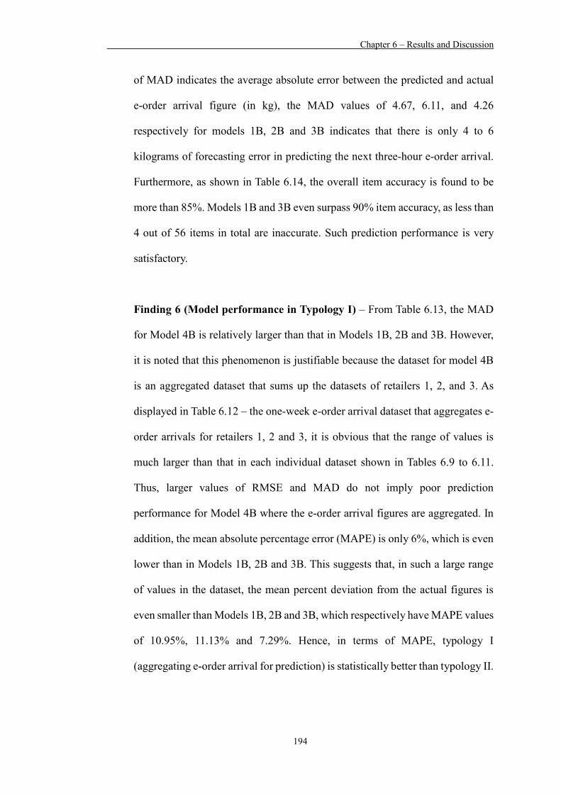
Chapter 6 – Results and Discussion
194
of MAD indicates the average absolute error between the predicted and actual
e-order arrival figure (in kg), the MAD values of 4.67, 6.11, and 4.26
respectively for models 1B, 2B and 3B indicates that there is only 4 to 6
kilograms of forecasting error in predicting the next three-hour e-order arrival.
Furthermore, as shown in Table 6.14, the overall item accuracy is found to be
more than 85%. Models 1B and 3B even surpass 90% item accuracy, as less than
4 out of 56 items in total are inaccurate. Such prediction performance is very
satisfactory.
Finding 6 (Model performance in Typology I) – From Table 6.13, the MAD
for Model 4B is relatively larger than that in Models 1B, 2B and 3B. However,
it is noted that this phenomenon is justifiable because the dataset for model 4B
is an aggregated dataset that sums up the datasets of retailers 1, 2, and 3. As
displayed in Table 6.12 – the one-week e-order arrival dataset that aggregates e-
order arrivals for retailers 1, 2 and 3, it is obvious that the range of values is
much larger than that in each individual dataset shown in Tables 6.9 to 6.11.
Thus, larger values of RMSE and MAD do not imply poor prediction
performance for Model 4B where the e-order arrival figures are aggregated. In
addition, the mean absolute percentage error (MAPE) is only 6%, which is even
lower than in Models 1B, 2B and 3B. This suggests that, in such a large range
of values in the dataset, the mean percent deviation from the actual figures is
even smaller than Models 1B, 2B and 3B, which respectively have MAPE values
of 10.95%, 11.13% and 7.29%. Hence, in terms of MAPE, typology I
(aggregating e-order arrival for prediction) is statistically better than typology II.

Chapter 6 – Results and Discussion
195
Table 6.13. Error analysis for model comparison for Model 1B to 4B
Model performance comparison Typology I II II II
Error measures: 4B 1B 2B 3B RMSE 12.73 5.42 7.42 5.14 MAD 9.92 4.67 6.11 4.26
MAPE (%) 6.00% 10.95% 11.13% 7.29%
Table 6.14. Item accuracy comparison for Model 1B to 4B
Model performance comparison Typology I II II II
Model 4B 1B 2B 3B No. of accurate items 56* 53+ 49+ 52+
No. of inaccurate items 0 3 7 4 Total number of items 56 56 56 56
Item accuracy 100% 94.6% 87.5% 92.9% + There are a total of 56 observations in a one-week dataset. For individual dataset for each retailer, an observation with MAD less than 10 is considered to be accurate. * An observation with MAD less than 30 is considered to be accurate for Model 4B as the dataset aggregates 3 retailer’s data.
Fig. 6.15. A graphical comparison between actual and predicted e-order arrival
figures for retailer 1 under Typology II

Chapter 6 – Results and Discussion
196
Fig. 6.16. A graphical comparison between actual and predicted e-order arrival
figures for retailer 2 under Typology II
Fig. 6.17. A graphical comparison between actual and predicted e-order arrival
figures for retailer 3 under Typology II
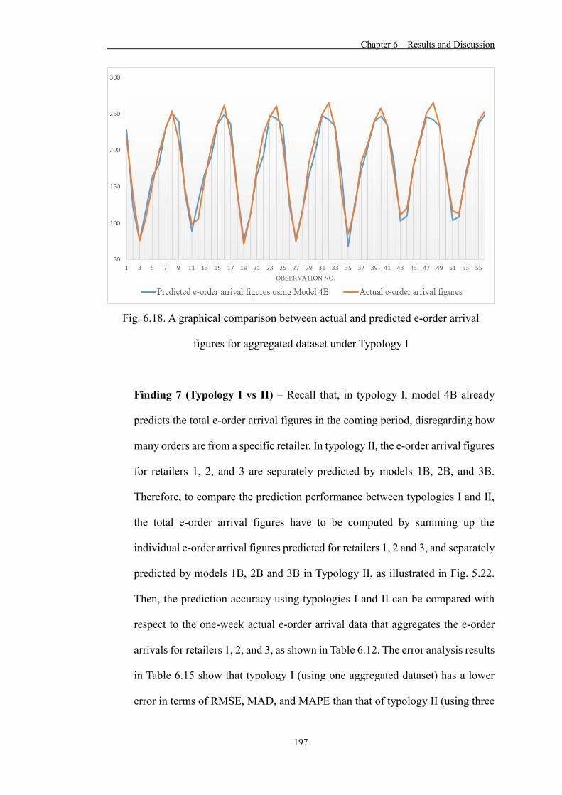
Chapter 6 – Results and Discussion
197
Fig. 6.18. A graphical comparison between actual and predicted e-order arrival
figures for aggregated dataset under Typology I
Finding 7 (Typology I vs II) – Recall that, in typology I, model 4B already
predicts the total e-order arrival figures in the coming period, disregarding how
many orders are from a specific retailer. In typology II, the e-order arrival figures
for retailers 1, 2, and 3 are separately predicted by models 1B, 2B, and 3B.
Therefore, to compare the prediction performance between typologies I and II,
the total e-order arrival figures have to be computed by summing up the
individual e-order arrival figures predicted for retailers 1, 2 and 3, and separately
predicted by models 1B, 2B and 3B in Typology II, as illustrated in Fig. 5.22.
Then, the prediction accuracy using typologies I and II can be compared with
respect to the one-week actual e-order arrival data that aggregates the e-order
arrivals for retailers 1, 2, and 3, as shown in Table 6.12. The error analysis results
in Table 6.15 show that typology I (using one aggregated dataset) has a lower
error in terms of RMSE, MAD, and MAPE than that of typology II (using three
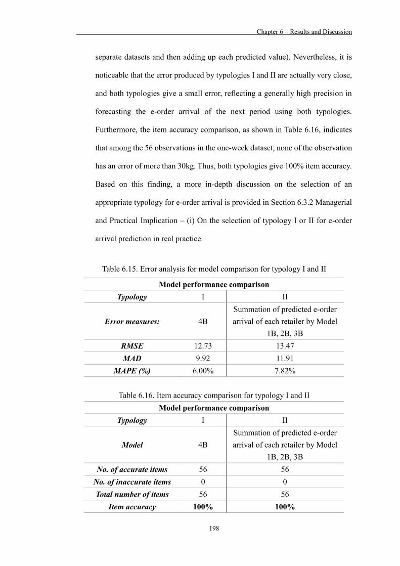
Chapter 6 – Results and Discussion
198
separate datasets and then adding up each predicted value). Nevertheless, it is
noticeable that the error produced by typologies I and II are actually very close,
and both typologies give a small error, reflecting a generally high precision in
forecasting the e-order arrival of the next period using both typologies.
Furthermore, the item accuracy comparison, as shown in Table 6.16, indicates
that among the 56 observations in the one-week dataset, none of the observation
has an error of more than 30kg. Thus, both typologies give 100% item accuracy.
Based on this finding, a more in-depth discussion on the selection of an
appropriate typology for e-order arrival is provided in Section 6.3.2 Managerial
and Practical Implication – (i) On the selection of typology I or II for e-order
arrival prediction in real practice.
Table 6.15. Error analysis for model comparison for typology I and II
Model performance comparison Typology I II
Error measures: 4B Summation of predicted e-order arrival of each retailer by Model
1B, 2B, 3B RMSE 12.73 13.47 MAD 9.92 11.91
MAPE (%) 6.00% 7.82%
Table 6.16. Item accuracy comparison for typology I and II Model performance comparison
Typology I II
Model 4B Summation of predicted e-order arrival of each retailer by Model
1B, 2B, 3B No. of accurate items 56 56
No. of inaccurate items 0 0 Total number of items 56 56
Item accuracy 100% 100%

Chapter 6 – Results and Discussion
199
(iii) Comparison 3 – Typology 1 vs Typology 2 for ARIMA model: ARIMA model
prediction performance comparison between typology 1 and 2
For effective prediction performance comparison between the ANFIS and
ARIMA approaches, the same eight-week data set used for training and testing the
ANFIS models, is also used for building the ARIMA(p,q)(r,s) model. The same as in
Case study 2, by selecting the maximum number of the autoregressive (AR), moving
average (MA), seasonal autoregressive (SAR) and seasonal moving average (SMA)
terms, say p, q, r, s, of the ARIMA model, as well as the periodicity of the seasonal
terms using EViews software package, one ARIMA model is built under typology I
for predicting the total e-order arrival, and three ARIMA models are built under
typology II for predicting the e-order arrival of retailers 1, 2, and 3 separately.
The best ARIMA model is automatically generated by the E-views software
package under each typology setting. Then, with the best ARIMA model generated,
another one-week historical data set, identically used in the ANFIS model evaluations,
which consists of a total of 56 e-order arrival figures in a three-hour interval, is used
for comparison of the ANFIS Models 1B, 2B, 3B, 4B and the ARIMA models.
Prediction performance of the ARIMA models are discussed below.
Typology I – Dataset aggregated all retailers’ data:
An ARIMA(4,4)(1,1) model, which obtains the lowest Akaike information criterion
(AIC) value, is selected after assessing 100 ARMA models, as shown in Fig. 6.19.
Dependent variables and the corresponding coefficients of the ARIMA(4,4)(1,1)
model are shown in Fig. 6.20. The ARIMA(4,4)(1,1) model is marked in red and is
graphically compared with the other ARMA models generated, as shown in Fig. 6.21.
A graphical comparison between actual and predicted e-order arrival figures of the
one-week dataset using ARIMA is presented in Fig. 6.22.

Chapter 6 – Results and Discussion
200
Fig. 6.19. Automatic ARIMA model selection result for the dataset aggregating all
retailers’ data
Fig. 6.20. Details of the ARIMA model selection result for the dataset aggregating all
retailers’ data

Chapter 6 – Results and Discussion
201
Fig. 6.21. Forecast comparison graph showing the selected model (in red) and other
ARIMA models (in grey) (for the dataset aggregating all retailers’ data)
Fig. 6.22. A graphical comparison between actual and predicted e-order arrival
figures using ARIMA for the dataset aggregating all retailers’ data
Typology II – Retailer 1’s dataset:
The same procedures as previously discussed apply to the other datasets. An
ARIMA(4,1)(1,1) model, which has the lowest Akaike information criterion (AIC)
value, is selected for retailer 1’s dataset after assessing 100 ARMA models, as shown
in Fig. 6.23. Dependent variables and the corresponding coefficients of the
ARIMA(4,1)(1,1) model are shown in Fig. 6.24. The ARIMA(4,1)(1,1) model is
marked in red and is graphically compared with other ARMA models generated, as

Chapter 6 – Results and Discussion
202
shown in Fig. 6.25. A graphical comparison between actual and predicted e-order
arrival figures of the one-week dataset using ARIMA is presented in Fig. 6.26.
Fig. 6.23. Automatic ARIMA model selection result for retailer 1’s dataset
Fig. 6.24. Details of the ARIMA model selection result for retailer 1’s dataset

Chapter 6 – Results and Discussion
203
Fig. 6.25. Forecast comparison graph showing the selected model (in red) and other
ARIMA models (in grey) (for retailer 1’s dataset)
Fig. 6.26. A graphical comparison between actual and predicted e-order arrival
figures using ARIMA for retailer 1
Typology II – Retailer 2’s dataset:
Similarly, an ARIMA(3,4)(1,1) model is generated and found to be the best one for
retailer’s 2 dataset. Details are shown in Figs. 6.27 to 6.30.

Chapter 6 – Results and Discussion
204
Fig. 6.27. Automatic ARIMA model selection result for retailer 2’s dataset
Fig. 6.28. Details of the ARIMA model selection result for retailer 2’s dataset
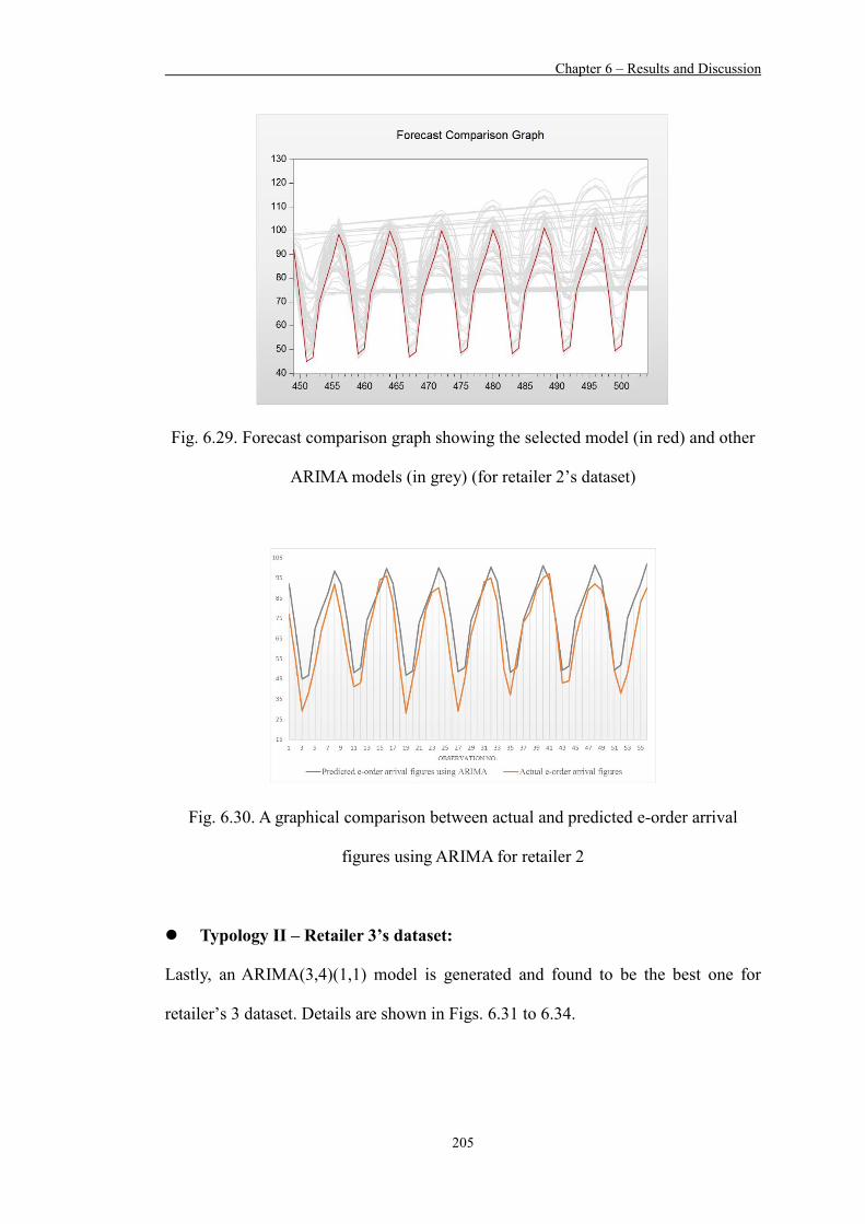
Chapter 6 – Results and Discussion
205
Fig. 6.29. Forecast comparison graph showing the selected model (in red) and other
ARIMA models (in grey) (for retailer 2’s dataset)
Fig. 6.30. A graphical comparison between actual and predicted e-order arrival
figures using ARIMA for retailer 2
Typology II – Retailer 3’s dataset:
Lastly, an ARIMA(3,4)(1,1) model is generated and found to be the best one for
retailer’s 3 dataset. Details are shown in Figs. 6.31 to 6.34.

Chapter 6 – Results and Discussion
206
Fig. 6.31. Automatic ARIMA model selection result for retailer 3’s dataset
Fig. 6.32. Details of the ARIMA model selection result for retailer 3’s dataset

Chapter 6 – Results and Discussion
207
Fig. 6.33. Forecast comparison graph showing the selected model (in red) and other
ARIMA models (in grey) (for retailer 3’s dataset)
Fig. 6.34. A graphical comparison between actual and predicted e-order arrival
figures using ARIMA for retailer 3
With the ARIMA models developed for each typology, error analysis is then
performed by comparing the predicted e-order arrival figures with respect to the one-
week actual dataset. The findings are discussed below.
Chapter 6 – Results and Discussion
208
Finding 8 (Typology I vs II in ARIMA) – In typology I, one ARIMA model is
generated using the dataset that aggregates all retailer’s e-order arrival data. In
typology II, three different ARIMA models are generated using each retailer’s
dataset to predict the e-order arrival figures of the corresponding retailers.
Therefore, to compare the prediction performance between typologies I and
II, the total e-order arrival figures have to be computed by summing up the
individual e-order arrival figures for retailers 1, 2 and 3 separately predicted by
ARIMA(4,1)(1,1), ARIMA(3,4)(1,1), and ARIMA(3,4)(1,1) in typology II.
Then, the prediction accuracy using typologies I and II can be compared with
respect to the one-week actual e-order arrival data that aggregates the e-order
arrival for retailers 1, 2 and 3, as shown in Table 6.12.
The error analysis results in Table 6.17 shows that typology I (using one
aggregated dataset) has a lower error in terms of RMSE, MAD, and MAPE than
that of typology II (using three separate datasets and then adding up each
predicted value), though it is noticeable that the errors produced by typologies I
and II are actually very close. Furthermore, the item accuracy comparison in
Table 6.18 also shows that typology I provides a slightly higher item accuracy.
Therefore, statistical error analysis suggests that typology I has a slightly better
prediction performance.

Chapter 6 – Results and Discussion
209
Table 6.17. Error analysis for ARIMA model comparison
Model performance comparison Typology I II II II II
ARIMA model:
ARIMA(4,4)(1,1) for dataset
aggregated all retailers
Summation of
separated forecasting
figures
ARIMA(4,1)(1,1) for Retailer 1
ARIMA(3,4)(1,1) for Retailer 2
ARIMA(3,4)(1,1) Retailer 3
RMSE 24.27 25.08 8.72 11.33 9.55 MAD 20.23 21.03 7.23 9.36 7.74
MAPE 13.82% 14.56% 18.41% 17.43% 16.81%
Table 6.18. Item accuracy comparison for ARIMA models
Model performance comparison Typology I II II II II
ARIMA model:
ARIMA (4,4)(1,1) for dataset aggregated all retailers
Summation of
separated forecasting
figures
ARIMA (4,1)(1,1)
for Retailer 1
ARIMA (3,4)(1,1)
for Retailer 2
ARIMA (3,4)(1,1)
for Retailer 3
No. of accurate items 44* 43* 45+ 35+ 40+ No. of inaccurate items 12 13 11 21 16
Total number of items 56 56 56 56 56
Item accuracy 78.6% 76.8% 80.4% 62.5% 71.4% + There are a total of 56 observations in a one-week dataset. For individual dataset for each retailer, an observation with MAD less than 10 is considered to be accurate. * An observation with MAD less than 30 is considered to be accurate for Model 4B as the dataset aggregates 3 retailer’s data.
(iv) Comparison 4 (the final comparison) – ANFIS vs ARIMA: Prediction
performance comparison between the ANFIS and ARIMA approaches
Finally, to compare the prediction performance between the proposed ANFIS and
the conventional ARIMA approach, several findings are identified, as discussed below:

Chapter 6 – Results and Discussion
210
Finding 9 (Model 1B to 4B vs ARIMA models in Typology II) – In typology
II, when retailers’ e-order arrival figures are separately forecasted by their
corresponding ANFIS and ARIMA models, the error analysis shown in Tables
6.19 and 6.20 clearly indicates that the ANFIS-based approach outperforms the
ARIMA-based approach, in terms of all error measures, i.e. RMSE, MAD,
MAPE, and item accuracy. Therefore, ANFIS is statistically proven to be a better
e-order arrival prediction model for predicting individual retailer’s e-order
arrival.
Table 6.19. Error analysis for ANFIS and ARIMA model comparison in typology II
Model performance comparison Retailer 1 Retailer 2 Retailer 3
Model: 1B ARIMA
(4,1)(1,1) 2B
ARIMA
(3,4)(1,1) 3B
ARIMA
(3,4)(1,1)
RMSE 5.42 8.72 7.42 11.33 5.14 9.55 MAD 4.67 7.23 6.11 9.36 4.26 7.74
MAPE 10.95% 18.41% 11.13% 17.43% 7.29% 16.81%
Table 6.20. Item accuracy comparison for ANFIS and ARIMA model comparison in
typology II
Model performance comparison Retailer 1 Retailer 2 Retailer 3
Model: 1B ARIMA
(4,1)(1,1) 2B
ARIMA
(3,4)(1,1) 3B
ARIMA
(3,4)(1,1)
No. of accurate items 53 45 49 35 52 40 No. of inaccurate items 3 11 7 21 4 16 Total number of items 56 56 56 56 56 56
Item accuracy 94.6% 80.4% 87.5% 62.5% 92.9% 71.4%

Chapter 6 – Results and Discussion
211
Finding 10 (ANFIS vs ARIMA) – Statistically, typology I (aggregating all
retailer’s datasets for prediction) has a slightly better prediction result than
typology II in both the ANFIS-based and ARIMA-based approaches. Therefore,
the ultimate comparison between ANFIS and ARIMA is by comparing the
prediction performance of ANFIS model in typology I with that of ARIMA
model in typology I. In other words, model 4B is compared with
ARIMA(4,4)(1,1).
As shown in Table 6.21, the error using ANFIS (Model 4B) is much lower
than that of ARIMA(4,4)(1,1), in terms of all error measures, i.e. RMSE, MAD
and MAPE. Interestingly, the RMSE, MAD and MAPE using ARIMA(4,4)(1,1)
are double of those using the ANFIS-based approach. Hence, the proposed
ANFIS-based approach gives a statistically 200% better prediction performance
than the conventional ARIMA model in forecasting e-order arrivals. As for item
accuracy comparison, as shown in Table 6.22, the ARIMA model also bares no
comparison with the proposed ANFIS model with only 78% item accuracy for
ARIMA and 100% item accuracy for ANFIS.
All in all, the proposed ANFIS approach that integrates the elements of
autoregressive (AR), momentum (MO) and moving average (MA) for model
construction is far better than the conventional ARIMA approach in forecasting
e-order arrival in distribution centres.
Table 6.21. Error analysis for ANFIS and ARIMA model comparison in typology I
Model performance comparison Approach ANFIS ARIMA
Model 4B ARIMA(4,4)(1,1) RMSE 12.73 24.27 MAD 9.92 20.23
MAPE (%) 6.00% 13.82%
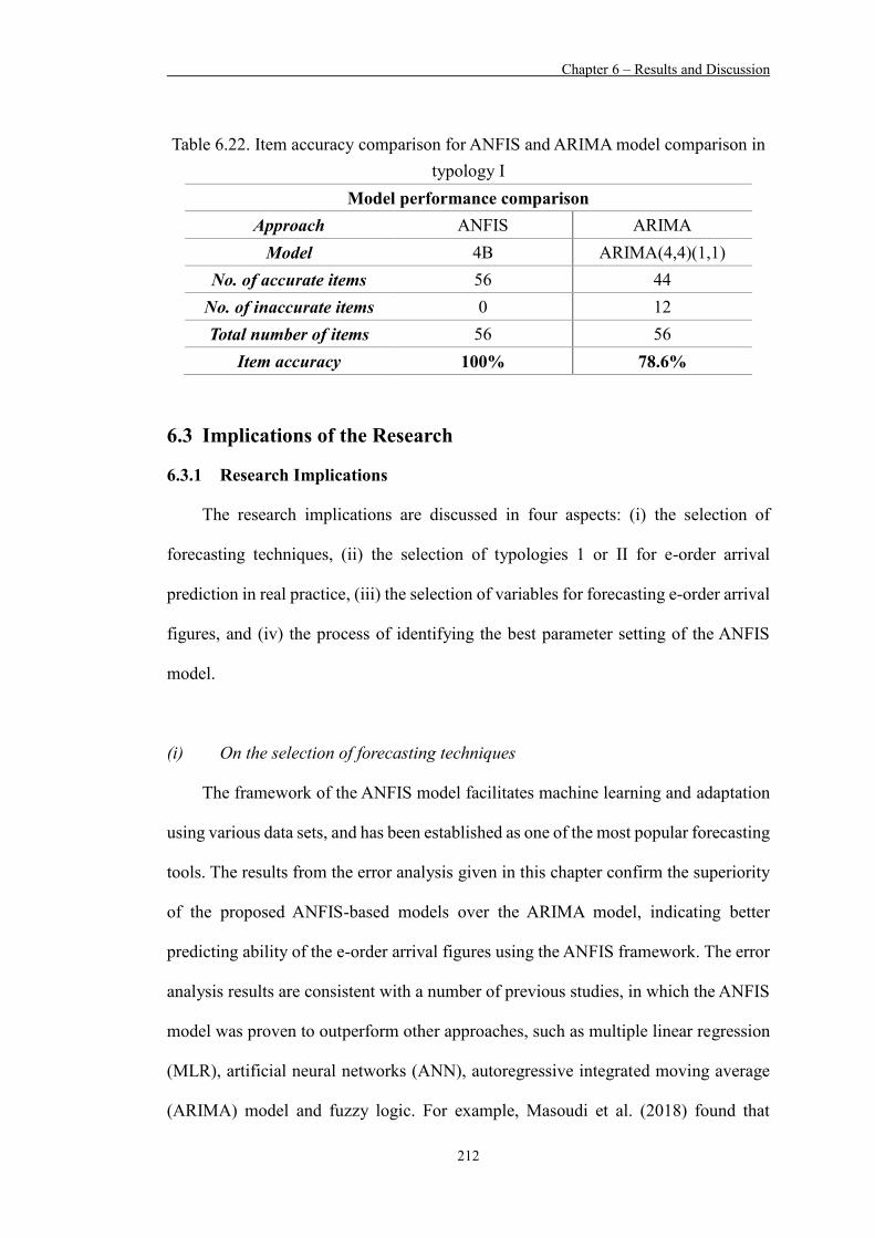
Chapter 6 – Results and Discussion
212
Table 6.22. Item accuracy comparison for ANFIS and ARIMA model comparison in
typology I Model performance comparison
Approach ANFIS ARIMA Model 4B ARIMA(4,4)(1,1)
No. of accurate items 56 44
No. of inaccurate items 0 12 Total number of items 56 56
Item accuracy 100% 78.6%
6.3 Implications of the Research
6.3.1 Research Implications
The research implications are discussed in four aspects: (i) the selection of
forecasting techniques, (ii) the selection of typologies 1 or II for e-order arrival
prediction in real practice, (iii) the selection of variables for forecasting e-order arrival
figures, and (iv) the process of identifying the best parameter setting of the ANFIS
model.
(i) On the selection of forecasting techniques
The framework of the ANFIS model facilitates machine learning and adaptation
using various data sets, and has been established as one of the most popular forecasting
tools. The results from the error analysis given in this chapter confirm the superiority
of the proposed ANFIS-based models over the ARIMA model, indicating better
predicting ability of the e-order arrival figures using the ANFIS framework. The error
analysis results are consistent with a number of previous studies, in which the ANFIS
model was proven to outperform other approaches, such as multiple linear regression
(MLR), artificial neural networks (ANN), autoregressive integrated moving average
(ARIMA) model and fuzzy logic. For example, Masoudi et al. (2018) found that

Chapter 6 – Results and Discussion
213
ANFIS models in general are more accurate than ANN in modelling manufacturing
processes and reflect the benefits of combining fuzzy systems capabilities with neural
networks. Tabrizi & Sancar (2017) compared three estimation models, MLR, ANN
and ANFIS. The results indicated that the ANFIS model for predicting Body Mass
Index is more feasible than the other two models. For instance, the ANFIS model also
performs well in handling time-series data. In this research, e-order arrival figures in
the distribution centre, as the prediction subject of this research, are time series data.
The prediction performance of the proposed ANFIS models suggests the suitability of
the ANFIS technique for the prediction of time series data. This indication is consistent
with a study performed by Efendigil et al. (2009), in which time series-type demand
in a supply chain was forecast using both artificial neural networks (ANN) and ANFIS,
and the ANFIS method was found to perform more effectively than the ANN approach
in the estimation of such time series data. This study, in conjunction with other ANFIS
literature, suggests that the ANFIS model is feasible for handling both time series and
non-time series data with accurate prediction performance.
(ii) On the selection of typologies I or II for e-order arrival prediction in real
practice
Finding 7 presented in the results and discussion part for Case study 3 (Section
6.2.3) shows that both typologies give an MAD of less than 12 kg. This indicates that
the difference in the actual and predicted e-order arrival figures for each three-hour
period is, on average, less than 12 kg. From the statistical point of view, typology I
(aggregating individual data for each retailer for prediction) performs slightly better
than typology II, with lower MAD, MAPE and RMSE error, as shown in Table 6.15.
However, both typologies in fact give very good prediction performance as both
typologies achieve 100% item accuracy (as shown in Table 6.16) and the error

Chapter 6 – Results and Discussion
214
difference between typologies I and II is very small, i.e. only an MAD of 2.01 kg, for
the e-order arrival figures (in kg) for the coming three-hour time interval.
From the statistical point of view, constructing one single ANFIS model for
aggregating e-order arrival figures is statistically justifiable for forecasting the e-order
arrival in distribution centres. Therefore, it can be concluded that aggregating e-order
arrivals for using one single ANFIS model for prediction provides a better prediction
accuracy.
In reality, managerial and practical implications of both prediction typologies (I
and II) need to be taken into consideration. It is noticeable that there are some
drawbacks of aggregating e-order arrival figures for prediction that cannot be ignored
from a practical perspective. In real practice, using only one single ANFIS model to
forecast the total e-order arrival disregards which retailer an e-order belongs to.
Without predicting an individual retailer’s e-order arrival, a logistics practitioner may
not be able to accurately allocate the right amount of resources to a specified zone
location in the distribution centre where the stock for a specific retailer is stored.
Therefore, this research suggests that, if there is a large number of retailers that the
logistics service provider has partnerships with, aggregating all retailers’ e-order
arrivals for forecasting a total e-order arrival (Typology I) in the coming period is more
appropriate, so as to reduce the effort in model construction, training and testing.
Otherwise, separately forecasting the e-order arrival of each retailer (Typology II) for
operational decision support for specific retailers enables the logistics service
providers to receive more benefits in ANFIS modelling. A summary of the practical
recommendation of the deployment of ANFIS forecasting models for e-order arrival
prediction is presented in Table 6.23.
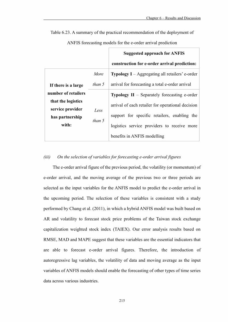
Chapter 6 – Results and Discussion
215
Table 6.23. A summary of the practical recommendation of the deployment of
ANFIS forecasting models for the e-order arrival prediction
Suggested approach for ANFIS
construction for e-order arrival prediction:
If there is a large
number of retailers
that the logistics
service provider
has partnership
with:
More
than 5
Typology I – Aggregating all retailers’ e-order
arrival for forecasting a total e-order arrival
Less
than 5
Typology II – Separately forecasting e-order
arrival of each retailer for operational decision
support for specific retailers, enabling the
logistics service providers to receive more
benefits in ANFIS modelling
(iii) On the selection of variables for forecasting e-order arrival figures
The e-order arrival figure of the previous period, the volatility (or momentum) of
e-order arrival, and the moving average of the previous two or three periods are
selected as the input variables for the ANFIS model to predict the e-order arrival in
the upcoming period. The selection of these variables is consistent with a study
performed by Chang et al. (2011), in which a hybrid ANFIS model was built based on
AR and volatility to forecast stock price problems of the Taiwan stock exchange
capitalization weighted stock index (TAIEX). Our error analysis results based on
RMSE, MAD and MAPE suggest that these variables are the essential indicators that
are able to forecast e-order arrival figures. Therefore, the introduction of
autoregressive lag variables, the volatility of data and moving average as the input
variables of ANFIS models should enable the forecasting of other types of time series
data across various industries.

Chapter 6 – Results and Discussion
216
(iv) On the process of identifying the best parameter setting of the ANFIS model
For practical deployment of the proposed ANFIS-based approach for order arrival
prediction, though industry practitioners are able to use autoregressive lag variables
and the volatility and moving average of data as the input parameters suggested in this
study to build their own ANFIS models for forecasting the order arrival rate in their
distribution centre, the best parameter settings for their own ANFIS models still need
to be identified through undergoing the five steps discussed in section 3.6.2 – ANFIS
Model Construction. Due to the fact that an ANFIS model can be built with a large
number of combination of settings, such as the type of membership function (MF), the
number of MFs for each input and the type of output function, ANFIS models under
different parameter settings can achieve very different results. Hence, identifying the
best parameter setting is a critical process when building an ANFIS model. To address
the essence of this process, this research presents a step-by-step framework for the
identification of the input variables, followed by how data sets are selected and split
into training and testing data sets, subsequently obtaining the best parameter setting
using the training and testing data sets. A detailed evaluation and error analysis of the
various settings is also presented in this chapter. Therefore, it is emphasized that there
is a crucial need to present not only the theoretical framework, but also the process of
obtaining the best parameter combination in detail for each of the proposed ANFIS
models, which is lacking in most of the ANFIS literature.
6.3.2 Managerial and Practical Implications
The managerial and practical implications are discussed in two aspects: (i) the essence
of reengineering the logistics flow for handling today’s e-commerce logistics orders,
(ii) the essence of integrating Information and Communication Technology (ICT) for

Chapter 6 – Results and Discussion
217
assisting logistics practitioners in the decision-making process for efficient e-order
handling.
(i) The essence of reengineering the logistics flow for handling today’s e-
commerce logistics orders
Making timely and accurate decisions depend not only on the availability of
information, but also how this is managed so as to select the proper data analytic tool
for extracting useful knowledge through gathering the raw data. The warehouse
postponement strategy, i.e. delaying the execution of a logistics process until the last
possible moment, can be executed in the real logistics environment only if an
appropriate data analytic tool provides industry practitioners with decision support for
determining the cut-off time of e-order groupings. Without such decision support,
industry practitioners are required to manually decide when to stop the consolidation
of e-commerce orders and subsequently release the consolidated orders for batch
processing in the distribution centre. It is a difficult decision to make in the absence of
any decision support, not to mention that the quality of such a manual decision cannot
be guaranteed. Worse still, improper timing in releasing grouped e-orders can severely
affect the efficiency in order handling and can create other resource allocation
problems, as shown in Table 6.24. For example, if the consolidated orders are released
too late, in other words, there are too many orders being grouped in this batch, the
grouped orders might need to be separated into more sub-batches as they cannot be
processed together at one time. Therefore, the proper timing for batch release is critical
for deploying an effective warehouse postponement strategy.
This study presents an ANFIS framework that is able to utilize the raw data of
historical e-order arrivals for forecasting the rate of e-order arrival in the upcoming
periods. By realizing the e-order arrival rate, the proposed system further generates

Chapter 6 – Results and Discussion
218
the optimal cut-off time of the pending e-orders, i.e. the remaining time to stop
consolidating discrete, small lot-sized e-commerce orders and release the consolidated
orders for processing in bulk in the distribution centre. In fact, apart from the optimal
cut-off time that can be generated based on the predicted e-order arrival rate, such
prediction can be further used for generating other types of decision support for
enhancing a firm’s operating performance or business competence. For example,
logistics practitioners can use the predicted e-order arrival figures for making other
warehouse related decisions, such as resource allocation decisions. Online retailers
can perform target marketing or design new promotional strategies, as they can now
realize the predicted number of e-orders that are to be placed by end consumers in the
e-marketplace in the upcoming time period.
Table 6.24. Various scenarios of ineffective warehouse postponement strategy
Consequences in the perspective of: Order handling Resource
management
If the consolidated orders were
released:
Too early
- Too few e-orders being grouped
- Lose the original idea of warehouse postponement
- Need to re-visit the same item storage location for many times due to a large number of order batches created
- Excessive resources remain idle
Too late
- Too many e-orders being grouped
- Unable to process the grouped orders at one time
- Need to separate the grouped orders into two or more batches
- Excessive workload of workers
Chapter 6 – Results and Discussion
219
(ii) The essence of integrating Information and Communication Technology (ICT)
for assisting logistics practitioners in the decision-making process for efficient
e-order handling
The rise of e-commerce, O2O retailing, and direct-to-consumer last-mile delivery
has positioned e-fulfilment distribution centers at the very heart of what end
consumers perceive as good service. Aggressive, guaranteed delivery dates are often
provided for addressing customer demands. The increasing convenience of online
shopping has redefined the way we shop; the customer demands, on the other hand,
are reshaping e-fulfilment. In the e-commerce marketplace, customer segmentation is
a known market opportunity enabling retailers to reach a wider customer base.
However, it is also one of the biggest challenges in e-commerce. The e-order fulfilment
of logistics service providers has to be very efficient in handling e-orders, which are
received from the internet at any time, and are to be delivered to a vast number of
locations worldwide by the guaranteed delivery dates. In the absence of decision
support systems facilitating the e-order internal processing operations in e-fulfilment
centers, logistics practitioners, especially those SME-sized organizations that often
handle orders without comprehensive IT support, experience obstacles in maintaining
the same level of efficiency as they had in handling traditional orders in warehouses
or distribution centers.
The evolution of information and communication technology (ICT) services with
cloud computing and mobile technologies has offered enterprises not only more sales
channels and effective formulation of target marketing strategies through big data
analytics, but also better internal and external information and communication
management solutions for integration into daily business for operational excellence.
However, with the slow pace of new technology adoption and innovation in the
logistics and distribution sector (Evangelista & Sweeney, 2006; European
Chapter 6 – Results and Discussion
220
Commission, 2012), logistics practitioners manage e-orders in a conventional flow of
operations, which affects their e-order handling capability and prolongs the e-
fulfilment lead time. The results from the case studies indicates that light-weight IT
applications that integrate artificial intelligence techniques and state-of-the-art cloud
computing technologies enable logistics practitioners to improve their internal order
processing in a cost effective manner. Software and solution providers should take e-
fulfilment requirements into consideration when designing and developing
competitive ICT solutions, with the integration of artificial intelligence techniques for
providing decision support and e-commerce logistics process re-engineering and
automation.
6.4 Summary
In this chapter, the results and discussion of the research are presented.
Experiments were performed for:
Identifying the best parameter settings for the GA algorithm in EGM of the EF-
DSS (Section 6.2.1),
Determining the best structure for the AR(1)MO(1) model and AR(1)MO(2)
models, and comparing the performance of the AR(1)MO(1) and AR(1)MO(2)
models with the traditional ARIMA (Section 6.2.2),
Determining the best structure for the AR(1)MO(1)MA(2) model and
AR(1)MO(1)MA(3) models, and comparing the performance of the AR(1)
MO(1)MA(2) and AR(1) MO(1)MA(3) models with the AR(1)MO(1) and
AR(1)MO(2) models and the traditional ARIMA (Section 6.2.3).
Finally, a number of significant implications in research, managerial, and
practical perspective are presented in this chapter.
Chapter 7 – Conclusions
221
Chapter 7 – Conclusions
7.1 Summary of the Research
The capability of logistics service providers in e-order fulfilment is one of the
key factors affecting the growth of the online retail business. This research study
develops an E-order Fulfilment Decision Support System (EF-DSS), which integrates:
(i) the genetic algorithm technique and the rule-based inference engine for logistics
service providers to effectively plan for the upcoming internal processing operations
of received orders before actual process execution, and (ii) ANFIS-based prediction
models for forecasting the arrival frequency of e-commerce orders so as to determine
the optimal timing for batch release of grouped orders. To provide the above-
mentioned decision support, the EF-DSS consists of three modules, namely E-order
Consolidation Module (ECM), E-order Grouping Module (EGM), and E-order Batch
Releasing Module (EBRM).
In ECM, an e-order consolidation pool is built using a cloud database for
consolidating pending e-orders. In EGM, an optimal internal order processing plan is
justified by the genetic algorithm approach. Essential operating guidance is provided
through the rule-based inference engine for order processing execution. With this
hybrid GA-rule-based approach enabling logistics service providers to determine
“How to group e-orders”, discrete e-orders are no longer required to be processed
immediately after they are received. The e-commerce internal order processing flow
is therefore streamlined and re-designed. The improved e-order handling capability of
logistics service providers eventually reduces the processing time in e-fulfilment
centers, thereby meeting the ever tighter delivery requirements of online customers.
Ultimately, the intelligent system presented in this research contributes to the
development of the e-commerce business environment from the perspective of the

Chapter 7 – Conclusions
222
interconnected parties. Logistics service providers become more capable in capturing
the logistics of the e-commerce business. Retailers can build brand images and loyalty
by satisfying the consumers’ needs and expectations, especially considering the
timeliness of the last-mile e-order delivery, one of the most critical e-fulfilment
processes. End consumers can receive their purchased items without a long waiting
time.
In EBRM, a novel ANFIS-based approach is proposed and developed with the
inclusion of the autoregressive, momentum and moving average characteristics of time
series data for the prediction of e-order arrival in distribution centres. Two typologies
are introduced to identify the best approach and set of ANFIS models for making
accurate prediction.
In summary, three case studies are undertaken to validate the performance of the
EF-DSS. Results upon implementation of EF-DSS in the case studies reveal the
feasibility of the EF-DSS in handling e-orders efficiently, and the superiority of ANFIS
models for forecasting the arrivals of e-orders in distribution centres.
7.2 Contributions of the Research
There are unprecedented pressures on companies to improve their operational
efficiency for enhanced competitiveness and overall business performance. Under the
fierce competition in the e-commerce operating environment, e-retailers are striving
to survive by attracting potential customers and retaining existing ones. To sustain
their core business, e-retailers who could also be the manufacturers of their listed
products, attempt to improve their competitive advantages by focusing on their core
business activities and outsourcing the non-core business functions, such as the
logistics and delivery segment to third-party logistics service providers (3PLs). This
has been a common phenomenon in the past decades. The essence of supply chain

Chapter 7 – Conclusions
223
integration in improving overall supply chain performance has been addressed in both
the academic and practitioner literature (Nguyen et al., 2018; Akter & Wamba, 2016;
Yu et al., 2016; Mellat-Parast & Spillan, 2014). In today’s fast-changing e-commerce
environment with tight customer requirements, particularly on speedy last-mile
delivery and the product availability, close connections and coordination must be
established among the stakeholders in the supply chain. For the outsourced functions
to be performed efficiently, e-retailers and 3PLs must closely co-operate. A standard
protocol for order information synchronization among e-retailers and 3PLs ought to
be established so as to streamline the information transmission process, increase the
information transparency, and extend the degree of information sharing, thus
achieving supply chain network excellence. 3PLs, on the other hand, need to utilize
the information shared by the e-retailers for effective order management. With the e-
commerce orders being fundamentally different from the conventional large lot-sized
stock replenishing orders in nature, and the fact that online customers are increasingly
emphasizing on order processing and delivery timeliness, the reputation of both the
3PL and the e-retailer hinges on the operating performance of the 3PL in handling the
e-orders in distribution centres.
In view of the need to streamline the e-commerce order fulfilment process, this
research provides a generic methodology for the development of an operation planning
system for effective order management under today’s e-commerce operating
environment. In general, the contributions of the research are threefold. They are:
(i) WPS – A novel operational methodology proposed in this research
The conventional product-oriented postponement strategy suggests practitioners
to “delay the production process until the last possible moment”, such as postponing
the product assembling operations for better product customization and meeting local

Chapter 7 – Conclusions
224
customer needs. The proposed operational strategy that should be applied in
distribution centres and warehouses, namely the Warehouse Postponement Strategy,
transforms the conventional product-oriented strategy into a process-oriented
operational strategy that is specifically designed for logistics practitioners. The
proposed strategy introduces the need to consolidate orders so as to delay the
subsequent order handling process, such as order pick-and-pack operations, until the
last possible moment. Such operational strategy is particularly applicable to LSPs who
handle a large number of e-commerce orders on a daily basis.
In the mainstream literature, research conducted in managing e-commerce order
fulfilment activities has been lacking (Nguyen et al., 2018). The environmental
implications and impact of e-commerce business on the related logistics activities have
not yet been studied in detail as well (Mangiaracina et al., 2015). The proposed WPS
fills the gap in the literature by introducing an operational strategy that takes the
environmental implications of e-commerce business into consideration in streamlining
e-order fulfillment activities. It is strongly recommended that more studies be
undertaken to remove the existing bottlenecks of e-commerce order fulfillment
operations, thereby proposing state-of-the-art solutions to tackle the problems
specifically found in e-fulfilment distribution centres where e-commerce orders are
processed.
(ii) EF-DSS – An intelligent decision support system developed in this research
that specifically take e-commerce operating bottlenecks into account
For effective execution of the proposed WPS, logistics practitioners are required
to consolidate orders with considerations of “How can the orders be grouped” and
“When should the grouped orders be released to distribution centres for batch
processing”. To provide a total solution for logistics practitioners to execute WPS in

Chapter 7 – Conclusions
225
real practice, this research combines the genetic algorithm technique, rule-based
inference engine, autoregressive modeling, and adaptive neuro-fuzzy inference system
(ANFIS). The EF-DSS developed in this research simultaneously tackles the problem
of “How to group the e-orders” and “When to release the grouped e-orders in a batch”
as identified at the beginning of this research, and is the first published study that
proposes the need to delay the execution of the order processes due to the fundamental
differences between e-order and conventional logistics order handling. It pinpoints the
two essential decisions to be made, i.e. how to group, and when to group e-orders,
under the wider concept of warehouse postponement, and thus provides specific
decision support for each of these decisions using artificial intelligence and machine
learning tools. The results upon deployment of the EF-DSS in three case studies in the
logistics service providers based in Hong Kong also indicate remarkable system and
operating performance.
(iii) Wide applicability of the proposed typologies for forecasting other time-series
data
This research takes the n-period autoregressive (AR), momentum (MO), moving
average (MA) indicators of time-series data into the account in the input variables
selection process of ANFIS forecasting models in the EBRM of the EF-DSS. These
input factors are generic characteristics of time-series data. Therefore, the proposed
ANFIS model typologies that integrate these generic characteristics of time-series data
suggest that the typologies proposed in this research and applied in the field of order
management in an e-commerce scenario may be appropriate for applications in
predicting subjects in other fields or industries. There is a wide range of potential areas
of application, where time-series data exist and can be used for prediction, thereby
generating knowledge and decision support in a particular field. A list of potential
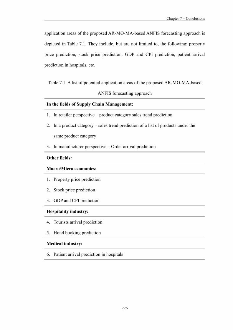
Chapter 7 – Conclusions
226
application areas of the proposed AR-MO-MA-based ANFIS forecasting approach is
depicted in Table 7.1. They include, but are not limited to, the following: property
price prediction, stock price prediction, GDP and CPI prediction, patient arrival
prediction in hospitals, etc.
Table 7.1. A list of potential application areas of the proposed AR-MO-MA-based
ANFIS forecasting approach
In the fields of Supply Chain Management:
1. In retailer perspective – product category sales trend prediction
2. In a product category – sales trend prediction of a list of products under the
same product category
3. In manufacturer perspective – Order arrival prediction
Other fields:
Macro/Micro economics:
1. Property price prediction
2. Stock price prediction
3. GDP and CPI prediction
Hospitality industry:
4. Tourists arrival prediction
5. Hotel booking prediction
Medical industry:
6. Patient arrival prediction in hospitals

Chapter 7 – Conclusions
227
7.3 Limitations of the Research and Suggestions for Future Work
Although this research makes significant contributions to both academia and the
logistics industry in today’s e-commerce business environment, there are some
limitations in the research and suggestions for future work as addressed below.
(i) Further strengthen the decision support algorithm “how to group” decision
decision using GA mechanism
In this research, the problem of grouping similar e-commerce orders is tackled
through the use of a GA algorithm. Depending on the operating parameters and
complexity of the e-order handling process of a logistics service provider, the GA
algorithm for generating “how to group” decision support can be strengthened in
future research.
(ii) Take more time-series characteristics into the consideration of process in
identifying the input variables of ANFIS forecasting technique
This research integrates n-period autoregressive (AR), momentum (MO), moving
average (MA) feature of time-series data for the modeling and construction of the
ANFIS forecasting approach for e-order arrival prediction. Despite this research
provides in-depth model comparison and evaluation using various time-series-type
input variables, and confirm their superiority over traditional forecasting approaches
in predicting e-commerce order arrival frequency, the inclusion of input variables
other than AR, MO and MA element is possible and can be considered in future.

Appendices
228
Appendices Appendix A. Evaluation and error analysis of various settings for AR(1)MO(1) model
Types of output function: No. of MFs for each input:
Constant Linear
Qd(t) Mo(t) Training
error Testing error
Training error
Testing error
2
2
TriMF 14.4271 14.427 14.0196 14.0196 TrapMF 14.0285 14.0278 13.0508 13.0507 GbellMF 13.8738 13.871 12.9082 12.9076 GuassMF 14.1305 14.1301 13.0306 13.0305
3
TriMF 14.3528 14.3527 13.7032 13.7032 TrapMF 14.8937 14.8926 12.8537 12.8535 GbellMF 14.2018 14.1988 12.5944 12.5939 GuassMF 14.2235 14.223 12.6902 12.6901
4
TriMF 14.2067 14.2066 13.4862 13.4862 TrapMF 13.7043 13.7038 12.4777 12.4771 GbellMF 13.6382 13.6361 12.3906 13.0284 GuassMF 13.895 13.8946 12.5762 12.5761
3
2
TriMF 13.9494 13.3703 12.8565 13.7287 TrapMF 14.7074 14.8646 12.8531 13.7465 GbellMF 14.1565 13.8674 12.7886 13.0672 GuassMF 14.0092 13.5464 12.8578 13.2057
3
TriMF 13.905 13.3784 12.5795 13.6921 TrapMF 15.6599 14.9848 12.8011 13.5483 GbellMF 14.5204 14.1298 12.6536 12.8613 GuassMF 14.1749 13.6863 12.5763 12.8562
4
TriMF 13.7233 13.263 12.3038 23.9326 TrapMF 14.7052 14.7565 12.5637 13.1572 GbellMF 14.1169 13.718 12.1552 14.5842 GuassMF 13.8971 13.3738 12.1517 13.818
4 2 TriMF 13.6765 13.0518 12.8329 13.4665 TrapMF 13.5524 13.0605 12.7256 13.3196 GbellMF 13.3704 12.961 12.6322 13.3313

Appendices
229
GuassMF 13.4527 12.9446 12.7332 13.4938
3
TriMF 13.481 12.7301 12.5223 13.3808 TrapMF 14.4935 13.5589 12.3381 14.8454 GbellMF 13.5491 12.8844 12.0301 13.4427 GuassMF 13.392 12.7344 12.1564 13.5443
4
TriMF 13.1496 12.9454 12.0825 14.0868 TrapMF 13.1139 13.1222 11.8162 13.4292 GbellMF 12.8147 12.6959 11.5945 14.8787 GuassMF 12.8882 12.4506 11.6623 15.4905
Appendix B. Evaluation and error analysis of various settings for AR(1)MO(2) model Types of output function: No. of MFs for each input:
Constant Linear
Qd(t) Mo(t) Mo(t-1) Training
error Testing error
Training error
Testing error
2
2
2
TriMF 13.648 13.0506 12.1941 11.2498 TrapMF 13.1712 12.3447 12.0434 11.52 GbellMF 13.1095 12.2946 11.7826 13.6268 GuassMF 13.3291 12.6148 11.8675 12.1885
3
TriMF 13.3267 12.8819 11.7977 13.0101 TrapMF 12.9524 12.6099 11.3156 14.7978 GbellMF 12.6675 12.1999 11.2045 10.9757 GuassMF 12.9037 12.3952 11.353 12.6964
4
TriMF 12.7593 13.0327 11.3698 11.7819 TrapMF 12.6124 11.8264 11.3551 12.5201 GbellMF 12.3754 12.6664 10.5341 14.4348 GuassMF 12.5097 12.7147 10.6357 14.1913
3
2
TriMF 13.358 12.3665 11.8545 11.6334 TrapMF 13.6353 13.6395 11.2878 11.5755 GbellMF 13.0861 12.1361 11.2439 13.1096 GuassMF 13.1414 12.0106 11.3146 12.3522
3 TriMF 12.9708 12.0729 10.921 12.7947 TrapMF 13.6294 14.1152 11.0043 17.3381 GbellMF 12.7659 12.6429 10.3535 20.3293
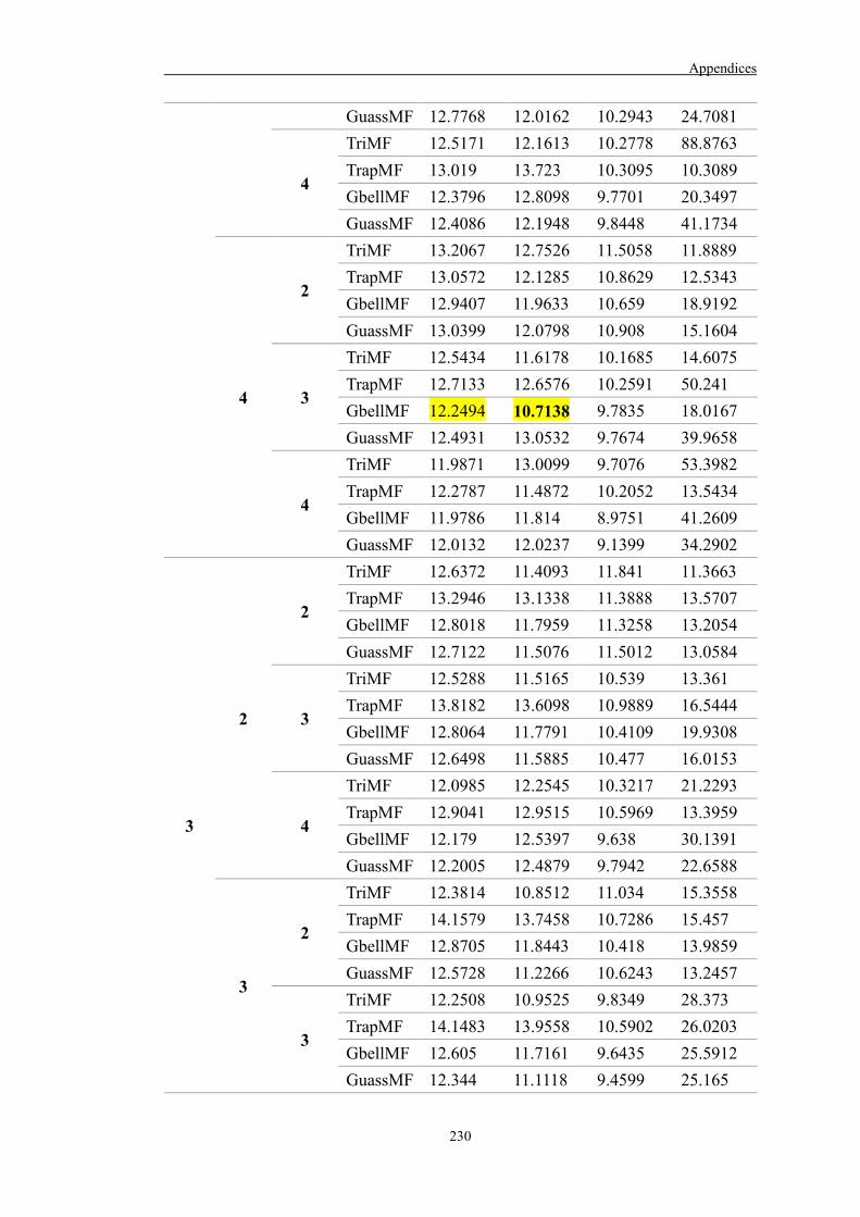
Appendices
230
GuassMF 12.7768 12.0162 10.2943 24.7081
4
TriMF 12.5171 12.1613 10.2778 88.8763 TrapMF 13.019 13.723 10.3095 10.3089 GbellMF 12.3796 12.8098 9.7701 20.3497 GuassMF 12.4086 12.1948 9.8448 41.1734
4
2
TriMF 13.2067 12.7526 11.5058 11.8889 TrapMF 13.0572 12.1285 10.8629 12.5343 GbellMF 12.9407 11.9633 10.659 18.9192 GuassMF 13.0399 12.0798 10.908 15.1604
3
TriMF 12.5434 11.6178 10.1685 14.6075 TrapMF 12.7133 12.6576 10.2591 50.241 GbellMF 12.2494 10.7138 9.7835 18.0167 GuassMF 12.4931 13.0532 9.7674 39.9658
4
TriMF 11.9871 13.0099 9.7076 53.3982 TrapMF 12.2787 11.4872 10.2052 13.5434 GbellMF 11.9786 11.814 8.9751 41.2609 GuassMF 12.0132 12.0237 9.1399 34.2902
3
2
2
TriMF 12.6372 11.4093 11.841 11.3663 TrapMF 13.2946 13.1338 11.3888 13.5707 GbellMF 12.8018 11.7959 11.3258 13.2054 GuassMF 12.7122 11.5076 11.5012 13.0584
3
TriMF 12.5288 11.5165 10.539 13.361 TrapMF 13.8182 13.6098 10.9889 16.5444 GbellMF 12.8064 11.7791 10.4109 19.9308 GuassMF 12.6498 11.5885 10.477 16.0153
4
TriMF 12.0985 12.2545 10.3217 21.2293 TrapMF 12.9041 12.9515 10.5969 13.3959 GbellMF 12.179 12.5397 9.638 30.1391 GuassMF 12.2005 12.4879 9.7942 22.6588
3
2
TriMF 12.3814 10.8512 11.034 15.3558 TrapMF 14.1579 13.7458 10.7286 15.457 GbellMF 12.8705 11.8443 10.418 13.9859 GuassMF 12.5728 11.2266 10.6243 13.2457
3
TriMF 12.2508 10.9525 9.8349 28.373 TrapMF 14.1483 13.9558 10.5902 26.0203 GbellMF 12.605 11.7161 9.6435 25.5912 GuassMF 12.344 11.1118 9.4599 25.165

Appendices
231
4
TriMF 11.5327 12.0992 9.4474 112.5874 TrapMF 13.6513 13.3607 10.085 35.4727 GbellMF 12.1045 12.85 8.7143 44.4161 GuassMF 11.8335 12.345 8.8267 56.6004
4
2
TriMF 12.1411 11.494 10.3637 12.3726 TrapMF 13.108 12.8297 10.1621 14.2853 GbellMF 12.3941 11.4939 9.7251 19.947 GuassMF 12.2553 11.233 9.8308 17.612
3
TriMF 11.9198 11.7827 8.8172 59.6185 TrapMF 13.7173 13.5359 9.5687 19.1148 GbellMF 12.2087 11.7067 8.7993 38.2297 GuassMF 11.9789 11.1917 8.7822 21.1079
4
TriMF 11.0019 14.5003 8.0621 77.1304 TrapMF 12.4708 11.9993 9.7111 14.0735 GbellMF 11.0135 12.8894 7.7649 45.2788 GuassMF 10.9409 14.0037 7.6939 63.4831
4
2
2
TriMF 12.7785 11.7943 11.1416 14.2183 TrapMF 12.6632 11.8873 10.9002 12.9608 GbellMF 12.5438 11.4684 10.8556 12.408 GuassMF 12.6088 11.4774 10.8669 12.9636
3
TriMF 12.5166 12.3103 10.1946 17.5911 TrapMF 12.5877 27.7602 10.4653 26.7841 GbellMF 12.1888 11.8186 9.9073 14.8401 GuassMF 12.2967 11.9344 9.8293 14.578
4
TriMF 11.9887 12.7546 9.4991 103.2905 TrapMF 11.7943 11.8035 10.0132 19.5224 GbellMF 11.6816 11.7824 9.1191 13.6296 GuassMF 11.7453 12.0145 9.1221 30.9574
3
2
TriMF 12.5321 11.4699 10.5653 13.1735 TrapMF 12.9196 13.6187 10.6645 19.6589 GbellMF 12.1674 11.8331 9.7487 15.1379 GuassMF 12.2793 11.4137 9.7912 17.4592
3
TriMF 12.1349 12.479 9.1298 16.1905 TrapMF 13.1509 14.9089 10.0839 212.4286 GbellMF 12.1281 12.3467 8.7511 31.7854 GuassMF 11.9803 12.1791 8.5484 20.2353
4 TriMF 11.4632 12.4465 8.1913 211.2479
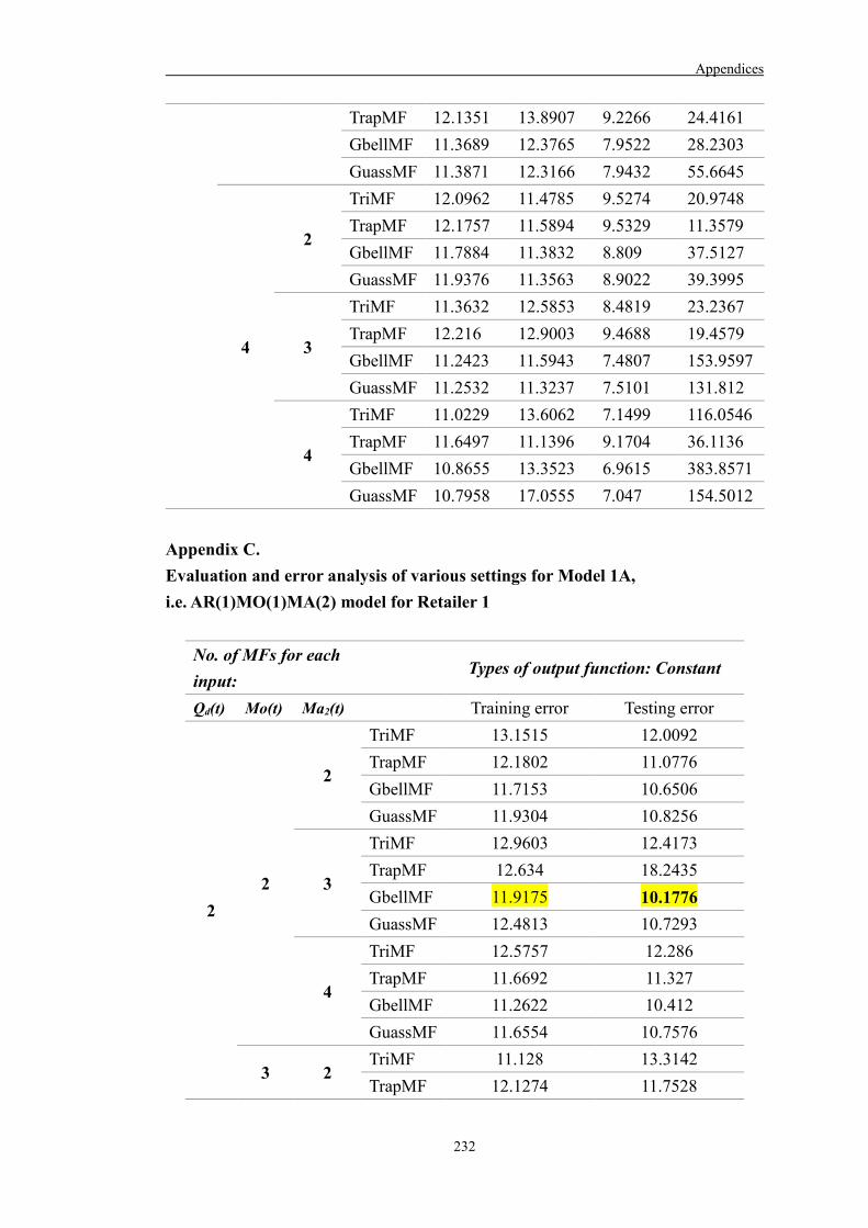
Appendices
232
TrapMF 12.1351 13.8907 9.2266 24.4161 GbellMF 11.3689 12.3765 7.9522 28.2303 GuassMF 11.3871 12.3166 7.9432 55.6645
4
2
TriMF 12.0962 11.4785 9.5274 20.9748 TrapMF 12.1757 11.5894 9.5329 11.3579 GbellMF 11.7884 11.3832 8.809 37.5127 GuassMF 11.9376 11.3563 8.9022 39.3995
3
TriMF 11.3632 12.5853 8.4819 23.2367 TrapMF 12.216 12.9003 9.4688 19.4579 GbellMF 11.2423 11.5943 7.4807 153.9597 GuassMF 11.2532 11.3237 7.5101 131.812
4
TriMF 11.0229 13.6062 7.1499 116.0546 TrapMF 11.6497 11.1396 9.1704 36.1136 GbellMF 10.8655 13.3523 6.9615 383.8571 GuassMF 10.7958 17.0555 7.047 154.5012
Appendix C. Evaluation and error analysis of various settings for Model 1A, i.e. AR(1)MO(1)MA(2) model for Retailer 1
No. of MFs for each input:
Types of output function: Constant
Qd(t) Mo(t) Ma2(t) Training error Testing error
2 2
2
TriMF 13.1515 12.0092 TrapMF 12.1802 11.0776 GbellMF 11.7153 10.6506 GuassMF 11.9304 10.8256
3
TriMF 12.9603 12.4173 TrapMF 12.634 18.2435 GbellMF 11.9175 10.1776 GuassMF 12.4813 10.7293
4
TriMF 12.5757 12.286 TrapMF 11.6692 11.327 GbellMF 11.2622 10.412 GuassMF 11.6554 10.7576
3 2 TriMF 11.128 13.3142 TrapMF 12.1274 11.7528

Appendices
233
GbellMF 10.899 11.4099 GuassMF 10.8047 10.7944
3
TriMF 10.5988 12.7924 TrapMF 13.1783 12.4371 GbellMF 11.164 11.4898 GuassMF 10.8635 11.4871
4
TriMF 10.6055 11.9072 TrapMF 12.348 14.5436 GbellMF 10.4755 11.7601 GuassMF 10.3144 11.4805
4
2
TriMF 10.4257 11.1526 TrapMF 11.6572 11.8984 GbellMF 10.8819 11.2482 GuassMF 10.7219 10.9287
3
TriMF 9.9282 11.9901 TrapMF 11.8873 12.2233 GbellMF 10.4572 10.5226 GuassMF 10.14 10.4463
4
TriMF 9.6213 10.3641 TrapMF 10.9503 12.7916 GbellMF 9.9397 10.5753 GuassMF 9.7447 10.6237
3
2
2
TriMF 12.6862 16.933 TrapMF 11.5498 11.6985 GbellMF 11.2636 10.7782 GuassMF 11.5786 11.1326
3
TriMF 12.0104 13.6739 TrapMF 12.3511 12.4265 GbellMF 11.1276 10.4194 GuassMF 11.4077 11.1987
4
TriMF 11.6155 15.3247 TrapMF 11.5002 12.3691 GbellMF 10.8989 10.6987 GuassMF 10.8466 11.1444
3 2 TriMF 10.7745 13.0429 TrapMF 13.5635 14.2505 GbellMF 11.8629 11.5446

Appendices
234
GuassMF 11.4221 11.2065
3
TriMF 10.513 12.7352 TrapMF 13.9237 13.534 GbellMF 9.9116 10.9391 GuassMF 9.9572 11.0661
4
TriMF 10.188 13.149 TrapMF 13.3765 13.747 GbellMF 10.003 11.5982 GuassMF 9.7191 11.541
4
2
TriMF 10.1108 11.3868 TrapMF 11.3256 12.6428 GbellMF 10.3489 11.4931 GuassMF 10.1335 11.0989
3
TriMF 9.8575 12.5177 TrapMF 11.7065 12.784 GbellMF 10.0124 10.2791 GuassMF 9.8481 10.976
4
TriMF 9.4146 11.1793 TrapMF 11.0384 13.3904 GbellMF 9.5685 11.7293 GuassMF 9.3202 10.9694
4
2
2
TriMF 12.252 17.4954 TrapMF 11.6383 10.6519 GbellMF 11.2983 10.945 GuassMF 11.7551 11.6921
3
TriMF 11.5353 13.4882 TrapMF 11.6656 11.785 GbellMF 10.5958 11.376 GuassMF 11.1847 10.6469
4
TriMF 11.6471 14.6402 TrapMF 11.0396 10.3426 GbellMF 10.2729 10.9845 GuassMF 10.2085 11.512
3 2
TriMF 10.6523 12.4104 TrapMF 11.9161 11.4996 GbellMF 10.9488 10.9648 GuassMF 10.6944 10.7899

Appendices
235
3
TriMF 10.3846 11.7688 TrapMF 12.0481 12.8981 GbellMF 10.3459 10.9339 GuassMF 10.3035 10.4624
4
TriMF 10.1513 12.8004 TrapMF 11.898 11.6072 GbellMF 9.6358 11.5273 GuassMF 9.5179 10.7315
4
2
TriMF 9.7469 10.8029 TrapMF 11.9913 11.4631 GbellMF 9.888 11.2058 GuassMF 9.8168 11.0841
3
TriMF 9.6253 12.7955 TrapMF 10.4063 12.5755 GbellMF 9.7064 11.7942 GuassMF 9.5378 12.0416
4
TriMF 9.3787 10.8492 TrapMF 10.2823 13.0534 GbellMF 9.382 12.9238 GuassMF 9.2407 11.7103
Appendix D. Evaluation and error analysis of various settings for Model 1B, i.e. AR(1)MO(1)MA(3) model for Retailer 1
No. of MFs for each input:
Types of output function: Constant
Qd(t) Mo(t) Ma3(t) Training error Testing error
2 2
2
TriMF 13.3285 11.6771 TrapMF 12.1317 10.3485 GbellMF 12.2179 10.5321 GuassMF 12.747 11.0181
3
TriMF 11.9845 11.8622 TrapMF 11.7481 10.4343 GbellMF 11.6044 10.4971 GuassMF 11.8187 10.8128
4 TriMF 12.382 11.8486

Appendices
236
TrapMF 11.619 11.4573 GbellMF 11.3627 11.018 GuassMF 11.752 11.395
3
2
TriMF 11.5872 10.5447 TrapMF 11.8556 11.7203 GbellMF 11.2267 10.9138 GuassMF 11.2953 10.5941
3
TriMF 10.817 11.1617 TrapMF 12.7665 11.0029 GbellMF 10.9622 11.2086 GuassMF 10.8476 10.982
4
TriMF 10.8296 10.3001 TrapMF 11.7925 11.6935 GbellMF 10.5668 10.517 GuassMF 10.5635 10.4175
4
2
TriMF 10.1881 9.2656 TrapMF 10.8889 10.7132 GbellMF 10.444 10.0762 GuassMF 10.306 9.7862
3
TriMF 9.6049 9.8867 TrapMF 10.9803 13.3816 GbellMF 9.8319 9.7877 GuassMF 9.5899 10.233
4
TriMF 9.4163 10.7883 TrapMF 10.6358 11.3201 GbellMF 9.5284 10.2981 GuassMF 9.2615 11.424
3 2
2
TriMF 12.6072 12.271 TrapMF 11.3408 10.8497 GbellMF 11.5463 10.7256 GuassMF 12.0439 11.3296
3
TriMF 10.8437 10.714 TrapMF 11.4072 14.19 GbellMF 10.3776 10.6676 GuassMF 10.4805 10.2498
4 TriMF 11.0571 10.996 TrapMF 11.1353 11.193

Appendices
237
GbellMF 10.3301 10.7445 GuassMF 10.4119 10.4194
3
2
TriMF 11.1322 10.5672 TrapMF 13.4138 12.757 GbellMF 11.5373 10.4813 GuassMF 11.1443 10.2459
3
TriMF 10.4049 10.8124 TrapMF 13.5947 13.0998 GbellMF 10.8773 10.5235 GuassMF 10.4487 10.6969
4
TriMF 10.4021 10.2736 TrapMF 13.5272 13.8355 GbellMF 10.3891 11.8172 GuassMF 10.1205 11.5497
4
2
TriMF 9.6486 9.3244 TrapMF 10.2131 12.3904 GbellMF 9.4025 10.5907 GuassMF 9.4114 10.1798
3
TriMF 9.1395 9.9152 TrapMF 10.9901 13.9781 GbellMF 9.273 10.5795 GuassMF 9.0581 10.484
4
TriMF 9.0718 10.8926 TrapMF 10.6337 11.9532 GbellMF 8.8883 11.0093 GuassMF 8.8374 12.5118
4 2
2
TriMF 11.8185 12.2359 TrapMF 10.832 10.1841 GbellMF 10.9275 10.4707 GuassMF 11.3155 11.16
3
TriMF 10.2174 10.8166 TrapMF 10.8364 10.2974 GbellMF 10.1346 9.895 GuassMF 10.1801 9.7666
4 TriMF 10.6126 11.2005 TrapMF 10.8393 11.3007 GbellMF 10.1676 9.6689
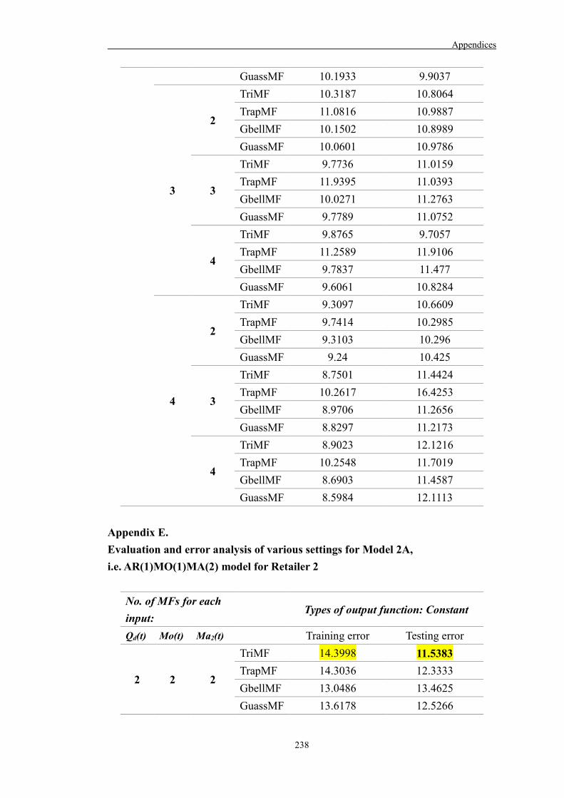
Appendices
238
GuassMF 10.1933 9.9037
3
2
TriMF 10.3187 10.8064 TrapMF 11.0816 10.9887 GbellMF 10.1502 10.8989 GuassMF 10.0601 10.9786
3
TriMF 9.7736 11.0159 TrapMF 11.9395 11.0393 GbellMF 10.0271 11.2763 GuassMF 9.7789 11.0752
4
TriMF 9.8765 9.7057 TrapMF 11.2589 11.9106 GbellMF 9.7837 11.477 GuassMF 9.6061 10.8284
4
2
TriMF 9.3097 10.6609 TrapMF 9.7414 10.2985 GbellMF 9.3103 10.296 GuassMF 9.24 10.425
3
TriMF 8.7501 11.4424 TrapMF 10.2617 16.4253 GbellMF 8.9706 11.2656 GuassMF 8.8297 11.2173
4
TriMF 8.9023 12.1216 TrapMF 10.2548 11.7019 GbellMF 8.6903 11.4587 GuassMF 8.5984 12.1113
Appendix E. Evaluation and error analysis of various settings for Model 2A, i.e. AR(1)MO(1)MA(2) model for Retailer 2
No. of MFs for each input:
Types of output function: Constant
Qd(t) Mo(t) Ma2(t) Training error Testing error
2 2 2
TriMF 14.3998 11.5383 TrapMF 14.3036 12.3333 GbellMF 13.0486 13.4625 GuassMF 13.6178 12.5266
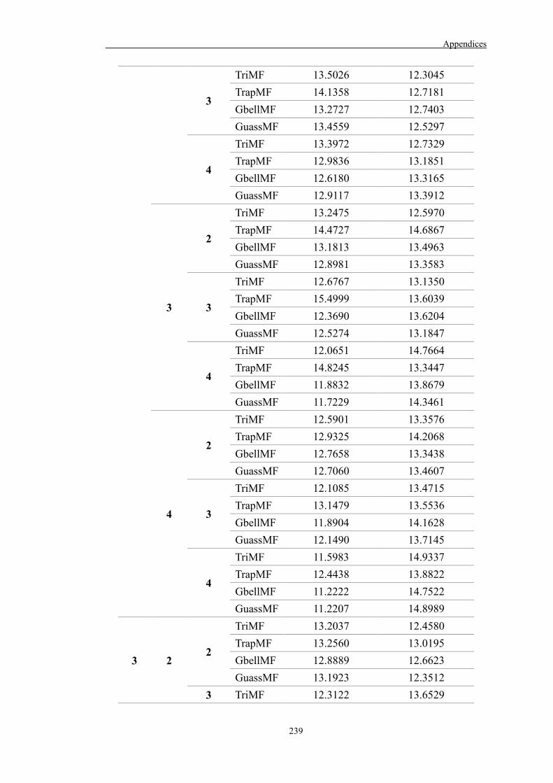
Appendices
239
3
TriMF 13.5026 12.3045 TrapMF 14.1358 12.7181 GbellMF 13.2727 12.7403 GuassMF 13.4559 12.5297
4
TriMF 13.3972 12.7329 TrapMF 12.9836 13.1851 GbellMF 12.6180 13.3165 GuassMF 12.9117 13.3912
3
2
TriMF 13.2475 12.5970 TrapMF 14.4727 14.6867 GbellMF 13.1813 13.4963 GuassMF 12.8981 13.3583
3
TriMF 12.6767 13.1350 TrapMF 15.4999 13.6039 GbellMF 12.3690 13.6204 GuassMF 12.5274 13.1847
4
TriMF 12.0651 14.7664 TrapMF 14.8245 13.3447 GbellMF 11.8832 13.8679 GuassMF 11.7229 14.3461
4
2
TriMF 12.5901 13.3576 TrapMF 12.9325 14.2068 GbellMF 12.7658 13.3438 GuassMF 12.7060 13.4607
3
TriMF 12.1085 13.4715 TrapMF 13.1479 13.5536 GbellMF 11.8904 14.1628 GuassMF 12.1490 13.7145
4
TriMF 11.5983 14.9337 TrapMF 12.4438 13.8822 GbellMF 11.2222 14.7522 GuassMF 11.2207 14.8989
3 2 2
TriMF 13.2037 12.4580 TrapMF 13.2560 13.0195 GbellMF 12.8889 12.6623 GuassMF 13.1923 12.3512
3 TriMF 12.3122 13.6529

Appendices
240
TrapMF 13.8290 12.5653 GbellMF 12.5468 13.9160 GuassMF 12.8487 13.1497
4
TriMF 12.5012 13.5758 TrapMF 12.7217 12.9977 GbellMF 12.2152 13.2103 GuassMF 11.9340 14.2880
3
2
TriMF 12.5450 13.5452 TrapMF 14.5970 14.8624 GbellMF 12.8847 13.1975 GuassMF 12.8170 13.3189
3
TriMF 11.6749 14.6799 TrapMF 14.7079 12.9802 GbellMF 11.9952 14.2222 GuassMF 11.8336 14.0465
4
TriMF 11.9125 15.0774 TrapMF 14.5737 13.8598 GbellMF 11.6714 14.0815 GuassMF 11.4274 14.7838
4
2
TriMF 12.0528 13.7527 TrapMF 12.5803 13.7913 GbellMF 12.0332 13.7940 GuassMF 11.9971 13.8994
3
TriMF 11.0454 15.1424 TrapMF 13.0700 13.7050 GbellMF 11.3965 15.3460 GuassMF 11.7694 14.2828
4
TriMF 11.0412 15.9151 TrapMF 12.4423 21.6795 GbellMF 11.1263 15.6520 GuassMF 11.1207 15.4167
4 2 2
TriMF 13.1769 12.3653 TrapMF 12.9478 13.2189 GbellMF 12.5002 13.4805 GuassMF 12.9363 12.8986
3 TriMF 12.6113 13.3123 TrapMF 13.6980 12.8870

Appendices
241
GbellMF 12.0395 14.2931 GuassMF 12.5949 13.2343
4
TriMF 12.3630 13.9285 TrapMF 12.5655 13.4957 GbellMF 11.7966 14.2921 GuassMF 11.9148 14.5747
3
2
TriMF 12.0153 14.2681 TrapMF 14.1344 14.1479 GbellMF 12.3438 13.6046 GuassMF 11.9867 13.7716
3
TriMF 11.8232 14.2400 TrapMF 14.3626 13.1858 GbellMF 11.7232 14.1200 GuassMF 11.6435 14.5794
4
TriMF 11.4895 15.7647 TrapMF 13.9390 12.8877 GbellMF 11.3794 16.0987 GuassMF 11.0414 14.9974
4
2
TriMF 11.5442 13.4632 TrapMF 12.5642 13.9687 GbellMF 11.5120 14.7590 GuassMF 11.5332 14.2628
3
TriMF 11.3274 14.4623 TrapMF 12.7109 14.3869 GbellMF 11.0208 15.6308 GuassMF 10.9752 15.4478
4
TriMF 10.7534 15.3114 TrapMF 12.1839 15.2000 GbellMF 10.8711 15.9224 GuassMF 10.7702 15.5959

Appendices
242
Appendix F. Evaluation and error analysis of various settings for Model 2B, i.e. AR(1)MO(1)MA(3) model for Retailer 2
No. of MFs for each input:
Types of output function: Constant
Qd(t) Mo(t) Ma3(t) Training error Testing error
2
2
2
TriMF 13.8957 11.1557 TrapMF 13.6854 11.8365 GbellMF 13.4167 11.6083 GuassMF 13.6817 11.3256
3
TriMF 12.7536 13.0986 TrapMF 12.2278 13.0045 GbellMF 12.0170 12.0439 GuassMF 12.1224 12.1862
4
TriMF 12.4913 12.1311 TrapMF 12.2496 12.5470 GbellMF 11.5497 12.6522 GuassMF 11.7845 12.6899
3
2
TriMF 12.8519 11.6571 TrapMF 14.8673 14.6439 GbellMF 13.1179 12.5875 GuassMF 12.8665 12.0819
3
TriMF 11.6920 12.8691 TrapMF 13.1771 16.0450 GbellMF 10.9032 14.3349 GuassMF 10.8767 13.7197
4
TriMF 11.4556 12.4071 TrapMF 14.0981 15.2762 GbellMF 10.9392 14.0651 GuassMF 11.0124 13.5921
4 2
TriMF 11.6301 13.6723 TrapMF 12.2490 16.3646 GbellMF 11.8939 13.7777 GuassMF 11.6714 13.5406
3 TriMF 10.8534 14.7281 TrapMF 11.3818 14.6695

Appendices
243
GbellMF 10.5556 14.0747 GuassMF 10.4290 14.3376
4
TriMF 10.6804 14.5866 TrapMF 11.3326 14.5580 GbellMF 10.3207 14.9455 GuassMF 10.3938 14.9628
3
2
2
TriMF 12.4250 12.1946 TrapMF 12.7330 12.6839 GbellMF 12.3067 12.5158 GuassMF 12.3865 12.3973
3
TriMF 11.6152 13.4787 TrapMF 12.4513 12.8763 GbellMF 11.5477 12.6061 GuassMF 11.4613 12.8771
4
TriMF 10.9984 13.2093 TrapMF 11.8814 13.9555 GbellMF 10.6989 13.3774 GuassMF 10.3618 13.9017
3
2
TriMF 11.8394 12.6296 TrapMF 13.8852 14.2184 GbellMF 12.3067 13.1732 GuassMF 11.9035 13.1910
3
TriMF 11.1508 12.8958 TrapMF 12.9463 14.6022 GbellMF 10.7671 14.3561 GuassMF 10.6836 13.9003
4
TriMF 10.6597 13.2210 TrapMF 13.6482 14.0915 GbellMF 10.1610 14.3567 GuassMF 10.1610 14.4742
4
2
TriMF 11.0724 14.1190 TrapMF 11.6262 12.9497 GbellMF 10.6606 14.2745 GuassMF 10.6690 14.4151
3 TriMF 10.5528 14.6133 TrapMF 12.0409 13.6703 GbellMF 10.0190 15.2198
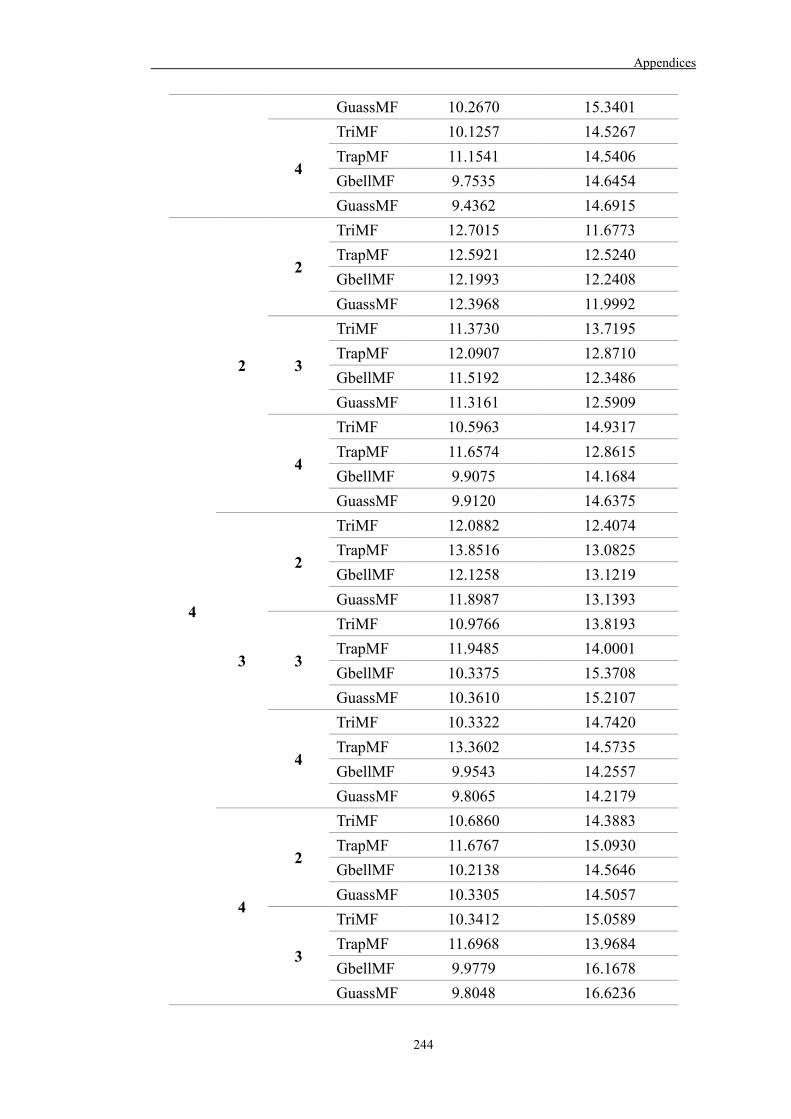
Appendices
244
GuassMF 10.2670 15.3401
4
TriMF 10.1257 14.5267 TrapMF 11.1541 14.5406 GbellMF 9.7535 14.6454 GuassMF 9.4362 14.6915
4
2
2
TriMF 12.7015 11.6773 TrapMF 12.5921 12.5240 GbellMF 12.1993 12.2408 GuassMF 12.3968 11.9992
3
TriMF 11.3730 13.7195 TrapMF 12.0907 12.8710 GbellMF 11.5192 12.3486 GuassMF 11.3161 12.5909
4
TriMF 10.5963 14.9317 TrapMF 11.6574 12.8615 GbellMF 9.9075 14.1684 GuassMF 9.9120 14.6375
3
2
TriMF 12.0882 12.4074 TrapMF 13.8516 13.0825 GbellMF 12.1258 13.1219 GuassMF 11.8987 13.1393
3
TriMF 10.9766 13.8193 TrapMF 11.9485 14.0001 GbellMF 10.3375 15.3708 GuassMF 10.3610 15.2107
4
TriMF 10.3322 14.7420 TrapMF 13.3602 14.5735 GbellMF 9.9543 14.2557 GuassMF 9.8065 14.2179
4
2
TriMF 10.6860 14.3883 TrapMF 11.6767 15.0930 GbellMF 10.2138 14.5646 GuassMF 10.3305 14.5057
3
TriMF 10.3412 15.0589 TrapMF 11.6968 13.9684 GbellMF 9.9779 16.1678 GuassMF 9.8048 16.6236

Appendices
245
4
TriMF 9.6418 15.8648 TrapMF 11.0448 14.3943 GbellMF 9.2461 14.3528 GuassMF 9.0671 15.4470
Appendix G. Evaluation and error analysis of various settings for Model 3A, i.e. AR(1)MO(1)MA(2) model for Retailer 3
No. of MFs for each input:
Types of output function: Constant
Qd(t) Mo(t) Ma2(t) Training error Testing error
2
2
2
TriMF 14.4693 11.2639 TrapMF 13.6159 12.2938 GbellMF 12.9924 11.7906 GuassMF 13.3282 11.6649
3
TriMF 13.7751 11.1240 TrapMF 13.2900 11.8759 GbellMF 12.8616 11.3161 GuassMF 13.0639 11.3323
4
TriMF 13.6759 11.1298 TrapMF 12.9829 11.2648 GbellMF 12.4482 10.9120 GuassMF 12.8427 10.9284
3
2
TriMF 12.6504 11.5262 TrapMF 13.4655 16.2689 GbellMF 12.0745 11.3669 GuassMF 12.3100 11.6025
3
TriMF 11.8633 11.6393 TrapMF 15.0365 12.7538 GbellMF 12.7072 11.2765 GuassMF 12.3295 11.6956
4
TriMF 11.4772 11.9664 TrapMF 13.5416 13.1191 GbellMF 11.8188 12.2097 GuassMF 11.6123 12.2186
4 2 TriMF 11.9767 12.0658

Appendices
246
TrapMF 12.6332 11.7351 GbellMF 12.1359 11.0784 GuassMF 12.1350 11.0909
3
TriMF 11.0450 11.5183 TrapMF 12.3776 12.7111 GbellMF 11.6151 11.5350 GuassMF 11.2194 11.4248
4
TriMF 10.8489 11.9304 TrapMF 11.7275 11.8352 GbellMF 10.8269 11.9122 GuassMF 10.7057 11.9634
3
2
2
TriMF 12.9161 11.4658 TrapMF 12.6571 11.3554 GbellMF 12.4395 10.9133 GuassMF 12.6624 10.8748
3
TriMF 12.3340 11.5042 TrapMF 13.1010 11.7401 GbellMF 12.0929 11.1906 GuassMF 11.8543 11.1536
4
TriMF 12.0881 11.7126 TrapMF 12.4882 12.0443 GbellMF 11.4583 11.5292 GuassMF 11.2140 11.8198
3
2
TriMF 12.0061 10.9272 TrapMF 14.9642 12.7801 GbellMF 13.1724 11.8778 GuassMF 12.8211 11.5110
3
TriMF 11.3336 11.6089 TrapMF 15.3373 12.8447 GbellMF 11.6485 11.7539 GuassMF 11.1369 11.6888
4
TriMF 10.8307 11.5176 TrapMF 15.0043 13.0727 GbellMF 11.0538 11.9738 GuassMF 10.8384 11.8641
4 2 TriMF 11.2374 11.7023 TrapMF 12.1486 12.0751
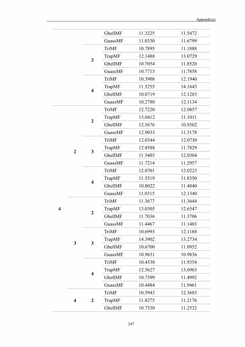
Appendices
247
GbellMF 11.3225 11.5472 GuassMF 11.0330 11.6799
3
TriMF 10.7895 11.1888 TrapMF 12.1488 13.0729 GbellMF 10.7054 11.8520 GuassMF 10.7715 11.7858
4
TriMF 10.3908 12.1940 TrapMF 11.5255 14.1643 GbellMF 10.0719 12.1283 GuassMF 10.2780 12.1134
4
2
2
TriMF 12.7220 12.0857 TrapMF 13.0412 11.1011 GbellMF 12.5676 10.9302 GuassMF 12.9033 11.3178
3
TriMF 12.0344 12.0730 TrapMF 12.8588 11.7829 GbellMF 11.5403 12.0304 GuassMF 11.7214 11.2957
4
TriMF 12.0701 12.0223 TrapMF 11.5519 11.8350 GbellMF 10.8022 11.4840 GuassMF 11.0315 12.1340
3
2
TriMF 11.3677 11.3644 TrapMF 13.0305 12.6547 GbellMF 11.7036 11.3706 GuassMF 11.4467 11.1403
3
TriMF 10.6993 12.1188 TrapMF 14.3902 13.2734 GbellMF 10.6700 11.0952 GuassMF 10.9631 10.9836
4
TriMF 10.4538 11.9354 TrapMF 12.5627 13.6963 GbellMF 10.7399 11.4992 GuassMF 10.4484 11.9461
4 2 TriMF 10.5943 12.3683 TrapMF 11.8275 11.2176 GbellMF 10.7330 11.2532

Appendices
248
GuassMF 10.7877 11.3499
3
TriMF 10.2240 11.9714 TrapMF 11.3989 13.1503 GbellMF 10.3732 11.4822 GuassMF 10.4476 11.1312
4
TriMF 10.0536 12.7101 TrapMF 10.6585 13.3506 GbellMF 9.7784 11.7145 GuassMF 10.1468 12.0611
Appendix H. Evaluation and error analysis of various settings for Model 3B, i.e. AR(1)MO(1)MA(3) model for Retailer 3
No. of MFs for each input:
Types of output function: Constant
Qd(t) Mo(t) Ma3(t) Training error Testing error
2
2
2
TriMF 13.9691 11.4841 TrapMF 13.6403 10.8385 GbellMF 13.3863 10.8947 GuassMF 13.7032 11.1526
3
TriMF 12.1098 11.1257 TrapMF 11.8903 11.2449 GbellMF 11.2711 10.7337 GuassMF 11.5234 10.6938
4
TriMF 12.5911 11.5778 TrapMF 12.5951 11.3254 GbellMF 12.0512 10.8094 GuassMF 12.1824 11.0090
3
2
TriMF 11.9435 11.4655 TrapMF 13.0168 13.2856 GbellMF 11.6025 12.1236 GuassMF 11.5283 11.9397
3
TriMF 11.1093 10.7682 TrapMF 13.3065 12.5737 GbellMF 10.5234 11.5262 GuassMF 10.5570 11.1690

Appendices
249
4
TriMF 10.5690 11.8199 TrapMF 12.5892 13.0719 GbellMF 10.4653 11.9181 GuassMF 10.3479 11.8301
4
2
TriMF 10.5023 12.3480 TrapMF 11.4966 11.7128 GbellMF 10.5768 11.8210 GuassMF 10.4290 12.0165
3
TriMF 10.0896 11.7194 TrapMF 11.3248 11.9560 GbellMF 10.0248 11.5356 GuassMF 10.0353 11.6113
4
TriMF 9.6724 11.8623 TrapMF 11.1261 12.3379 GbellMF 9.8756 11.6577 GuassMF 9.7289 11.4326
3
2
2
TriMF 12.5313 10.5077 TrapMF 12.3517 11.2067 GbellMF 11.9553 10.7050 GuassMF 12.2956 10.5939
3
TriMF 10.8656 10.3123 TrapMF 11.5582 12.0968 GbellMF 10.3825 11.6920 GuassMF 10.3901 11.1687
4
TriMF 11.1511 11.2423 TrapMF 11.7807 12.5861 GbellMF 10.4506 11.4335 GuassMF 10.0490 11.6926
3
2
TriMF 10.9738 10.9507 TrapMF 13.8155 12.1942 GbellMF 11.3660 11.6507 GuassMF 10.8949 11.4003
3
TriMF 10.6273 10.5008 TrapMF 13.7983 12.0556 GbellMF 10.5703 11.9598 GuassMF 10.3370 11.5696
4 TriMF 9.7798 11.8799

Appendices
250
TrapMF 13.9613 12.7496 GbellMF 10.3864 12.2207 GuassMF 9.8761 11.4765
4
2
TriMF 9.5482 11.6609 TrapMF 11.1066 11.7216 GbellMF 9.7940 11.5819 GuassMF 9.7073 11.6538
3
TriMF 9.1019 11.0467 TrapMF 10.6351 13.4041 GbellMF 9.3824 11.8962 GuassMF 9.1208 11.7303
4
TriMF 8.9653 11.3867 TrapMF 10.6470 12.7520 GbellMF 8.8875 11.4255 GuassMF 8.4482 11.0523
4
2
2
TriMF 12.6888 10.7319 TrapMF 12.3458 10.6811 GbellMF 12.0063 10.3066 GuassMF 12.2852 10.5115
3
TriMF 9.9229 10.9907 TrapMF 11.4195 12.1262 GbellMF 10.1691 11.6414 GuassMF 9.9798 11.4028
4
TriMF 10.8072 12.0473 TrapMF 11.7405 11.5443 GbellMF 9.9074 11.4857 GuassMF 9.7535 11.7627
3
2
TriMF 10.1939 12.1235 TrapMF 12.0061 12.8762 GbellMF 10.1370 11.8184 GuassMF 9.9357 11.9419
3
TriMF 9.6685 11.3135 TrapMF 12.5858 13.0107 GbellMF 9.8176 11.7620 GuassMF 9.6221 11.4419
4 TriMF 9.4106 12.2614 TrapMF 12.1269 13.0490
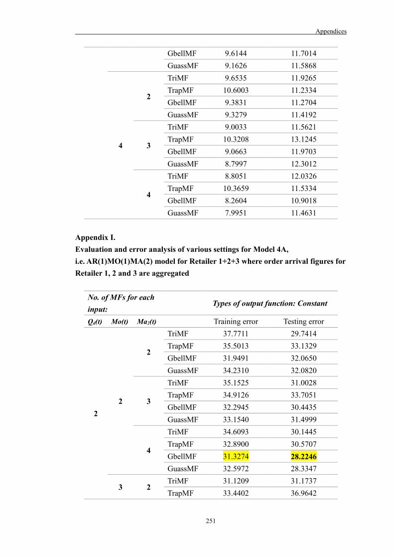
Appendices
251
GbellMF 9.6144 11.7014 GuassMF 9.1626 11.5868
4
2
TriMF 9.6535 11.9265 TrapMF 10.6003 11.2334 GbellMF 9.3831 11.2704 GuassMF 9.3279 11.4192
3
TriMF 9.0033 11.5621 TrapMF 10.3208 13.1245 GbellMF 9.0663 11.9703 GuassMF 8.7997 12.3012
4
TriMF 8.8051 12.0326 TrapMF 10.3659 11.5334 GbellMF 8.2604 10.9018 GuassMF 7.9951 11.4631
Appendix I. Evaluation and error analysis of various settings for Model 4A, i.e. AR(1)MO(1)MA(2) model for Retailer 1+2+3 where order arrival figures for Retailer 1, 2 and 3 are aggregated
No. of MFs for each input:
Types of output function: Constant
Qd(t) Mo(t) Ma2(t) Training error Testing error
2 2
2
TriMF 37.7711 29.7414 TrapMF 35.5013 33.1329 GbellMF 31.9491 32.0650 GuassMF 34.2310 32.0820
3
TriMF 35.1525 31.0028 TrapMF 34.9126 33.7051 GbellMF 32.2945 30.4435 GuassMF 33.1540 31.4999
4
TriMF 34.6093 30.1445 TrapMF 32.8900 30.5707 GbellMF 31.3274 28.2246 GuassMF 32.5972 28.3347
3 2 TriMF 31.1209 31.1737 TrapMF 33.4402 36.9642

Appendices
252
GbellMF 30.1771 33.2900 GuassMF 30.1497 32.0298
3
TriMF 28.8430 30.0207 TrapMF 37.7959 35.3432 GbellMF 30.1269 30.6355 GuassMF 29.7762 30.3419
4
TriMF 25.5409 31.9664 TrapMF 34.4029 39.6396 GbellMF 27.0118 34.7674 GuassMF 26.3110 33.8983
4
2
TriMF 29.7317 32.0540 TrapMF 30.9428 33.7764 GbellMF 28.9683 30.6947 GuassMF 29.4817 31.2889
3
TriMF 26.1971 29.6256 TrapMF 30.1612 31.7667 GbellMF 25.9952 31.7454 GuassMF 26.1172 29.8903
4
TriMF 24.1102 31.2327 TrapMF 27.2220 34.4056 GbellMF 24.0447 30.9296 GuassMF 23.8856 31.3405
3
2
2
TriMF 33.0971 31.9886 TrapMF 31.9228 29.7260 GbellMF 30.6329 28.9870 GuassMF 31.3824 29.7189
3
TriMF 30.2330 32.8590 TrapMF 35.0554 33.6221 GbellMF 29.1483 31.6450 GuassMF 29.8347 32.7649
4
TriMF 30.2846 29.1719 TrapMF 30.0930 61.4093 GbellMF 27.2389 33.7140 GuassMF 27.0964 35.0796
3 2 TriMF 28.2449 31.1303 TrapMF 38.0883 38.2237 GbellMF 31.9944 30.5122
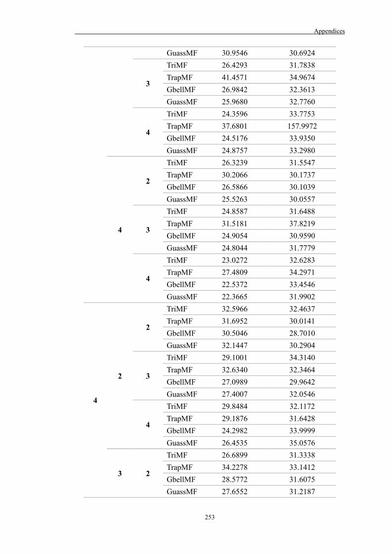
Appendices
253
GuassMF 30.9546 30.6924
3
TriMF 26.4293 31.7838 TrapMF 41.4571 34.9674 GbellMF 26.9842 32.3613 GuassMF 25.9680 32.7760
4
TriMF 24.3596 33.7753 TrapMF 37.6801 157.9972 GbellMF 24.5176 33.9350 GuassMF 24.8757 33.2980
4
2
TriMF 26.3239 31.5547 TrapMF 30.2066 30.1737 GbellMF 26.5866 30.1039 GuassMF 25.5263 30.0557
3
TriMF 24.8587 31.6488 TrapMF 31.5181 37.8219 GbellMF 24.9054 30.9590 GuassMF 24.8044 31.7779
4
TriMF 23.0272 32.6283 TrapMF 27.4809 34.2971 GbellMF 22.5372 33.4546 GuassMF 22.3665 31.9902
4
2
2
TriMF 32.5966 32.4637 TrapMF 31.6952 30.0141 GbellMF 30.5046 28.7010 GuassMF 32.1447 30.2904
3
TriMF 29.1001 34.3140 TrapMF 32.6340 32.3464 GbellMF 27.0989 29.9642 GuassMF 27.4007 32.0546
4
TriMF 29.8484 32.1172 TrapMF 29.1876 31.6428 GbellMF 24.2982 33.9999 GuassMF 26.4535 35.0576
3 2
TriMF 26.6899 31.3338 TrapMF 34.2278 33.1412 GbellMF 28.5772 31.6075 GuassMF 27.6552 31.2187

Appendices
254
3
TriMF 24.1298 35.9261 TrapMF 37.5707 32.5203 GbellMF 24.9437 35.6530 GuassMF 24.9677 32.8281
4
TriMF 23.5289 32.5790 TrapMF 32.8850 37.9708 GbellMF 23.5226 34.6061 GuassMF 22.9912 33.3830
4
2
TriMF 24.5383 33.3301 TrapMF 28.6065 30.4290 GbellMF 24.0717 30.7144 GuassMF 24.1908 31.8722
3
TriMF 23.2414 33.6718 TrapMF 27.6866 33.5366 GbellMF 22.3005 33.0594 GuassMF 22.7798 32.1008
4
TriMF 22.4259 35.9409 TrapMF 25.1930 35.4917 GbellMF 20.9080 34.2562 GuassMF 21.4624 34.3788
Appendix J. Evaluation and error analysis of various settings for Model 4B, i.e. AR(1)MO(1)MA(3) model for Retailer 1+2+3 where order arrival figures for Retailer 1, 2 and 3 are aggregated
No. of MFs for each input:
Types of output function: Constant
Qd(t) Mo(t) Ma3(t) Training error Testing error
2 2
2
TriMF 37.1960 37.1959 TrapMF 34.6317 29.5271 GbellMF 34.3474 28.2751 GuassMF 35.9787 29.0726
3
TriMF 31.9749 34.9142 TrapMF 30.7342 33.2349 GbellMF 30.3697 32.0101 GuassMF 31.1201 32.3838
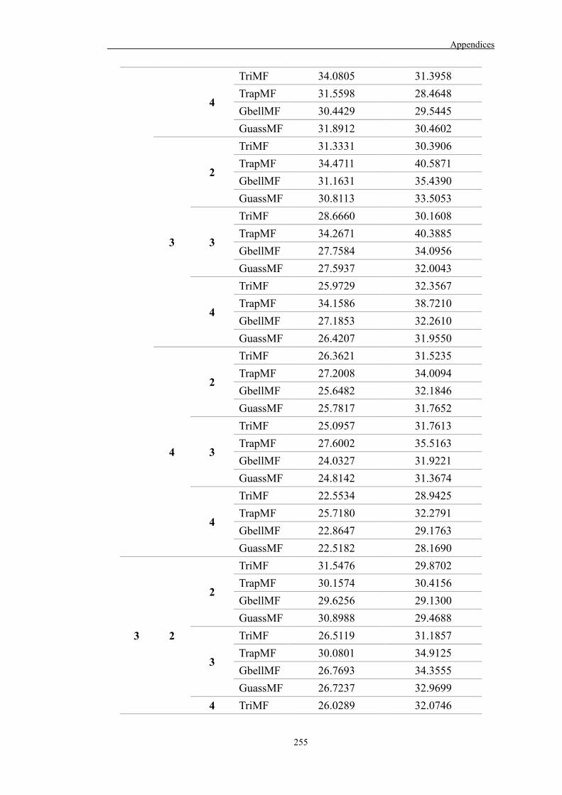
Appendices
255
4
TriMF 34.0805 31.3958 TrapMF 31.5598 28.4648 GbellMF 30.4429 29.5445 GuassMF 31.8912 30.4602
3
2
TriMF 31.3331 30.3906 TrapMF 34.4711 40.5871 GbellMF 31.1631 35.4390 GuassMF 30.8113 33.5053
3
TriMF 28.6660 30.1608 TrapMF 34.2671 40.3885 GbellMF 27.7584 34.0956 GuassMF 27.5937 32.0043
4
TriMF 25.9729 32.3567 TrapMF 34.1586 38.7210 GbellMF 27.1853 32.2610 GuassMF 26.4207 31.9550
4
2
TriMF 26.3621 31.5235 TrapMF 27.2008 34.0094 GbellMF 25.6482 32.1846 GuassMF 25.7817 31.7652
3
TriMF 25.0957 31.7613 TrapMF 27.6002 35.5163 GbellMF 24.0327 31.9221 GuassMF 24.8142 31.3674
4
TriMF 22.5534 28.9425 TrapMF 25.7180 32.2791 GbellMF 22.8647 29.1763 GuassMF 22.5182 28.1690
3 2
2
TriMF 31.5476 29.8702 TrapMF 30.1574 30.4156 GbellMF 29.6256 29.1300 GuassMF 30.8988 29.4688
3
TriMF 26.5119 31.1857 TrapMF 30.0801 34.9125 GbellMF 26.7693 34.3555 GuassMF 26.7237 32.9699
4 TriMF 26.0289 32.0746

Appendices
256
TrapMF 27.8146 55.5373 GbellMF 24.5478 31.2448 GuassMF 24.0847 32.8908
3
2
TriMF 28.0162 30.8895 TrapMF 36.6376 34.4445 GbellMF 30.7247 31.8831 GuassMF 28.8704 31.4578
3
TriMF 26.0655 30.0482 TrapMF 35.1542 34.8745 GbellMF 27.4649 34.6092 GuassMF 26.4827 31.7786
4
TriMF 23.6312 34.6039 TrapMF 37.7357 35.8491 GbellMF 25.8721 34.7604 GuassMF 24.8266 33.5007
4
2
TriMF 23.7671 32.0337 TrapMF 26.6314 29.7041 GbellMF 22.8027 31.6851 GuassMF 22.9748 31.4599
3
TriMF 21.9494 31.5020 TrapMF 28.1056 36.4831 GbellMF 21.6338 32.1236 GuassMF 21.4890 31.5915
4
TriMF 20.5724 30.6597 TrapMF 23.9835 30.2716 GbellMF 20.0916 31.0390 GuassMF 19.6246 29.5022
4 2
2
TriMF 32.6374 30.4187 TrapMF 30.3525 27.8652 GbellMF 30.4547 27.4482 GuassMF 31.6127 28.7692
3
TriMF 25.8668 32.8113 TrapMF 28.4831 35.7053 GbellMF 25.4697 33.6931 GuassMF 25.7193 33.1815
4 TriMF 26.4427 33.3037 TrapMF 28.3899 27.8913
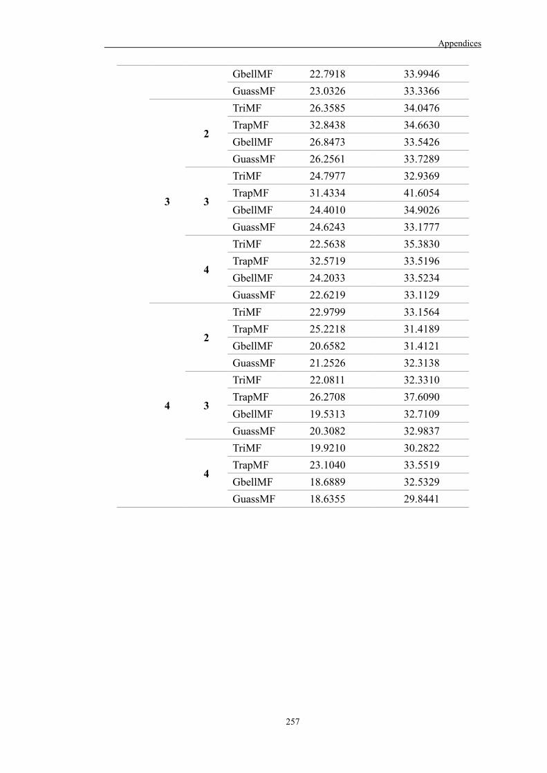
Appendices
257
GbellMF 22.7918 33.9946 GuassMF 23.0326 33.3366
3
2
TriMF 26.3585 34.0476 TrapMF 32.8438 34.6630 GbellMF 26.8473 33.5426 GuassMF 26.2561 33.7289
3
TriMF 24.7977 32.9369 TrapMF 31.4334 41.6054 GbellMF 24.4010 34.9026 GuassMF 24.6243 33.1777
4
TriMF 22.5638 35.3830 TrapMF 32.5719 33.5196 GbellMF 24.2033 33.5234 GuassMF 22.6219 33.1129
4
2
TriMF 22.9799 33.1564 TrapMF 25.2218 31.4189 GbellMF 20.6582 31.4121 GuassMF 21.2526 32.3138
3
TriMF 22.0811 32.3310 TrapMF 26.2708 37.6090 GbellMF 19.5313 32.7109 GuassMF 20.3082 32.9837
4
TriMF 19.9210 30.2822 TrapMF 23.1040 33.5519 GbellMF 18.6889 32.5329 GuassMF 18.6355 29.8441

References
258
References
Aamodt, A. and Plaza, E. (1994). Case-based reasoning: foundational issues,
methodological variations, and system approaches. AICom – Artificial
Intelligence Communications, 7(1), 39-59.
Abhishek, V., Jerath, K., & Zhang, Z. J. (2015). Agency selling or reselling? Channel
structures in electronic retailing. Management Science, 62(8), 2259-2280.
Accorsi, R., Manzini, R., & Maranesi, F. (2014). A decision-support system for the
design and management of warehousing systems. Computers in Industry, 65(1)
pp. 175-186.
Admuthe, L. S., & Apte, S. (2010). Adaptive neuro-fuzzy inference system with
subtractive clustering: a model to predict fiber and yarn relationship. Textile
Research Journal, 80(9), 841-846.
Aengchuan, P., & Phruksaphanrat, B. (2018). Comparison of fuzzy inference system
(FIS), FIS with artificial neural networks (FIS+ ANN) and FIS with adaptive
neuro-fuzzy inference system (FIS+ ANFIS) for inventory control. Journal of
Intelligent Manufacturing, 29(4), 905-923.
Agatz, N.A., Fleischmann, M., & Van Nunen, J.A. (2008). E-fulfillment and multi-
channel distribution: a review. European Journal of Operational Research, 187,
pp. 339–356.
Agrawal, R., Imieliński, T., Swami, A. (1993). Mining association rules between sets
of items in large databases. Proceedings of the 1993 ACM SIGMOD international
conference on Management of data - SIGMOD '93. 207.
Ahmad, M. W., Mourshed, M., & Rezgui, Y. (2017). Trees vs Neurons: Comparison
between random forest and ANN for high-resolution prediction of building energy
consumption. Energy and Buildings, 147, 77-89.

References
259
Akcayol, M. A. (2004). Application of adaptive neuro-fuzzy controller for SRM.
Advances in Engineering Software, 35(3–4), 129–137.
Akhter, F., Hobbs, D., & Maamar, Z. (2005). A fuzzy logic-based system for assessing
the level of business-to-consumer (B2C) trust in electronic commerce. Expert
Systems with Applications, 28(4), 623-628.
Akter, S., & Wamba, S. F. (2016). Big data analytics in E-commerce: a systematic
review and agenda for future research. Electronic Markets, 26(2), 173-194.
Al-Harbi, K. M. A. S. (2001). Application of the AHP in project management.
International Journal of Project Management, 19(1), 19-27.
Alrashed, A. A., Gharibdousti, M. S., Goodarzi, M., de Oliveira, L. R., Safaei, M. R.,
& Bandarra Filho, E. P. (2018). Effects on thermophysical properties of carbon
based nanofluids: Experimental data, modelling using regression, ANFIS and
ANN. International Journal of Heat and Mass Transfer, 125, 920-932.
Altug, S., Chow, M.Y., & Trussell, H.J. (1999). Fuzzy inference systems. implemented
on neural architectures for motor. IEEE Transactions on Industrial Electronics,
46 (6), 1069-1079.
ARC Advisory Group, 'Warehouse Management Systems ARC Advisory Group',
Retrieved 29/12/14 World Wide Web, http://www.arcweb.com/market-
studies/pages/warehouse-management-systems.aspx.
Areerachakul, S. (2012). Comparison of ANFIS and ANN for estimation of
biochemical oxygen demand parameter in surface water. International Journal of
Chemical and Biological Engineering, 6, 286-290.
Armbrust, M., Fox, A., Griffith, R., Joseph, A.D., Katz, R., Konwinski, A., Lee, G.,
Patterson, D., Rabkin, A., Stoica, I. and Zaharia, M. (2010). A view of Cloud
computing. Communications of the ACM, 53(4), 50 – 58.

References
260
Attaran, M. (2007). RFID: an enabler of supply chain operations. Supply Chain
Management: An International Journal, 12(4), 249-257.
Autry, C.W., Grawe, S.J., Daugherty, P. and Richey, R.G. Jr (2010). The effects of
technological turbulence and breadth on supply chain technology acceptance and
adoption. Journal of Operations Management, 28(6), 522-36.
Avci, E. (2008). Comparison of wavelet families for texture classification by using
wavelet packet entropy adaptive network based fuzzy inference system. Applied
Soft Computing, 8(1), 225–231.
Avci, E., Hanbay, D., & Varol, A. (2007). An expert discrete wavelet adaptive network
based fuzzy inference system for digital modulation recognition. Expert Systems
with Applications, 33(3), 582–589.
Azadeh, A., Asadzadeh, S. M., Saberi, M., Nadimi, V., Tajvidi, A., & Sheikalishahi,
M. (2011). A neuro-fuzzy-stochastic frontier analysis approach for long-term
natural gas consumption forecasting and behavior analysis: the cases of Bahrain,
Saudi Arabia, Syria, and UAE. Applied Energy, 88(11), 3850-3859.
Badger, L., Grance, T., Patt-Corner, P. and Voas, J. (2011). Draft-Cloud Computing
Synopsis and Recommendations. National Institute of Standards and Technology,
Gaithersburg, MD, May.
Ballou, R.H. (1999). Business Logistics Management. Prentice-Hall, Englewood
Cliffs, NJ.
Barbosa, Hisano D. and Musetti, Andreotti M. (2010). Logistics information systems
adoption: an empirical investigation in Brazil. Industrial Management & Data
Systems, 110(6), 787-804.
Battini, D., Calzavara, M., Persona, A., & Sgarbossa, F. (2015). Order picking system
design: the storage assignment and travel distance estimation (SA&TDE) joint
method. International Journal of Production Research, 53(4), 1077-1093.
References
261
Berg, J., and Zijm, W. (1999). Models for warehouse management: Classification and
examples. International Journal of Production Economics, 59(1-3), 519-528.
Billah, B., King, M.L., Snyder, R.D.& Koehler, A.B. (2006). Exponential smoothing
model. selection for forecasting. International Journal of Forecasting, 22, 239-
247.
Bindi, F., Manzini, R., Pareschi, A., & Regattieri, A. (2009). Similarity-based storage
allocation rules in an order picking system: an application to the food service
industry. International Journal of Logistics Research and Applications, 12(4),
pp.233-247.
Bloom, J. Z. (2005). Market segmentation: A neural network application. Annals of
Tourism Research, 32(1), 93-111.
Boone, C., Craighead, C., & Hanna, J. (2007). Postponement: an evolving supply
chain concept. International Journal of Physical Distribution & Logistics
Management, 37(8), 594-611.
Bowersox, D.J., Closs, D.J. and Stank, T.P. (1999). 21st Century Logistics: Making
Supply Chain Integration a Reality. Council of Logistics Management, Oak
Brook, IL.
Box, G.& Jenkins, G. (1976). Time Series Analysis: Forecasting and Control. Holden-
Day.
Boyacioglu, M. A., & Avci, D. (2010). An adaptive network-based fuzzy inference
system (ANFIS) for the prediction of stock market return: the case of the Istanbul
stock exchange. Expert Systems with Applications, 37(12), 7908-7912.
Boyer, K.K. and Hult, G.T.M. (2005). Extending the supply chain: integrating
operations and marketing in the online grocery industry. Journal of Operations
Management, 23(6), 642-61.
References
262
Brézillon, P. et al. (2000), SART: An Intelligent Assistant System for Subway Control.
Pesquisa Operacional. 20(2), 247-268.
Bridgman, P. W. (1922). Dimensional analysis. Yale University Press.
Brown, R.G. (1959). Statistical Forecasting for Inventory Control. McGraw-Hill,
New York
Brown, R.G. (1963). Smoothing, Forecasting and prediction of Discrete Time Series.
Prentice-Hall, Englewood Cliffs.
Buyya, R., Vecchiola, C. and Selvi, S. (2013). Mastering cloud computing. Waltham,
MA: Morgan Kaufmann.
Cabeza, M., & Moilanen, A. (2001). Design of reserve networks and the persistence
of biodiversity. Trends in ecology & evolution, 16(5), 242-248.
Can, F., Altingövde, I. S., & Demir, E. (2004). Efficiency and effectiveness of query
processing in cluster-based retrieval. Information Systems, 29(8), 697-717.
Cao, M., Luo, X., Luo, X. R., & Dai, X. (2015). Automated negotiation for e-
commerce decision making: a goal deliberated agent architecture for multi-
strategy selection. Decision Support Systems, 73, 1-14.
Cardona, L. F., Soto, D. F., Rivera, L., & Martínez, H. J. (2015). Detailed design of
fishbone warehouse layouts with vertical travel. International Journal of
Production Economics, 170, 825-837.
Carlson, J., O’Cass, A., & Ahrholdt, D. (2015). Assessing customers’ perceived value
of the online channel of multichannel retailers: A two country examination.
Journal of Retailing and Consumer Services, 27, 90-102.
Caron, F., Marchet, G., & Perego, A. (2000). Optimal Layout in Low-Level Picker-to-
Part Systems. International Journal of Production Research, 38, 101-117.

References
263
Castro-Schez, J., Miguel, R., Vallejo, D., & López-López, L. (2011). A highly adaptive
recommender system based on fuzzy logic for B2C e-commerce portals. Expert
Systems with Applications, 38(3), 2441-2454.
Census and Statistics Department. (2003), Hong Kong Monthly Digest of Statistics.
December 2013. Hong Kong, pp. 1-16.
Chan, F., & Kumar, V. (2009). Hybrid TSSA algorithm-based approach to solve
warehouse-scheduling problems. International Journal of Production Research,
47(4), 919-940.
Chan, H., He, H., & Wang, W. (2012). Green marketing and its impact on supply chain
management in industrial markets. Industrial Marketing Management, 41(4), 557-
562.
Chang, J. R., Wei, L. Y., & Cheng, C. H. (2011). A hybrid ANFIS model based on AR
and volatility for TAIEX forecasting. Applied Soft Computing, 11(1), 1388-1395.
Chen, B., & Lee, C. (2008). Logistics scheduling with batching and transportation.
European Journal of Operational Research, 189(3), 871-876.
Chen, J., & Shen, X. L. (2015). Consumers' decisions in social commerce context: An
empirical investigation. Decision Support Systems, 79, 55-64.
Chen, M., Zhang, D. and Zhou, L. (2007). Empowering collaborative commerce with
web services enabled business process management systems, Decision Support
Systems, 43(2), 530-546.
Chen, X., & Lin, H. (2013). Research on e-commerce logistics system
informationization in chain. Procedia-social and behavioral sciences, 96, 838-
843.
Chew, E. P., & Tang, L.C. (1999). Travel time analysis for general item location
assignment in a rectangular warehouse. European Journal of Operational
Research, 112, 582–597.
References
264
Chi, R.T., Chen, M. and Kiang, M.Y. (1993). Generalized case-based reasoning system
for portfolio management. Expert Systems with Applications, 6, 67-76.
Chia Jane, C. (2000), Storage location assignment in a distribution center,
International Journal of Physical Distribution & Logistics Management, 30 (1),
pp. 55-71.
Chiu, S. L. (1994). Fuzzy model identification based on cluster estimation. Journal of
Intelligent and Fuzzy Systems, 2, 267–278.
Cho, Jay Joong‐Kun, Ozment, J., & Sink, H. (2008). Logistics capability, logistics
outsourcing and firm performance in an e‐commerce market. International
Journal of Physical Distribution & Logistics Management, 38(5), 336 – 359.
Cho, V. (2003). A comparison of three different approaches to tourist arrival
forecasting. Tourism management, 24(3), 323-330.
Choi, K., Narasimhan, R., & Kim, S. (2012). Postponement strategy for international
transfer of products in a global supply chain: A system dynamics examination.
Journal of Operations Management, 30(3), 167-179.
Chow, Harry K.H., Choy, K.L., Lee, W.B., & Lau, K.C. (2006). Design of a RFID
case-based resource management system for warehouse operations. Expert
Systems with Applications, 30(4), 561-576, 2006.
Chow, H.K.H., Choy, K.L., Lee, W.B. and Chan, F.T.S. (2007). Integration of web‐
based and RFID technology in visualizing logistics operations – a case study.
Supply Chain Management: An International Journal, 12(3), 221-234.
Choy, K. L., Lee, W. B., Lau, H. C., & Choy, L. C. (2005). A knowledge-based supplier
intelligence retrieval system for outsource manufacturing. Knowledge-based
systems, 18(1), 1-17.
Christopher, M. (2016). Logistics & supply chain management. Pearson UK.

References
265
CLM (2004). Definition of logistics. Council of Logistics Management, available at:
www.cscmp.org/
Craw, S., Wiratunga, N. and Rowe, R. (2006). Learning adaptation knowledge to
improve case-based reasoning. Artificial Intelligence, 170(16-17), 1175-1192.
Crum, M.R., Premkumar, G. and Ramamurthy, K. (1996). An assessment of motor
carrier adoption, use and satisfaction with EDI. Transportation Journal, 35(4),
44‐57.
Cunnane, Chris. (2015). E-Commerce Growth Brings Last Mile Headaches. Logistics
Viewpoints, ARC Advisory Group. [Online]. Available: http://www.
http://logisticsviewpoints.com/ [Accessed: 15 July, 2015]
Cybenko, G. (1989). Approximation by superpositions of a sigmoidal function.
Mathematics of control, signals and systems, 2(4), 303-314.
Davenport, T.H., and Brooks, J.D. (2004). Enterprise systems and the supply chain.
Journal of Enterprise Information Management, 17(1), pp. 8-19.
Davidsson, Paul et al. (2005). An Analysis of Agent-Based Approaches to Transport
Logistics. Transportation Research Part C: Emerging Technologies, 13(4), pp.
255-271.
De Koster, M., Van der Poort, E., & Wolters, M. (1999). Efficient order batching
methods in warehouses. International Journal of Production Research, 37(7), pp.
1479-1504.
De Koster, R.B.M. (2003). Distribution strategies for online retailers. IEEE
Transactions on Engineering Management, 50, 448–457.
De Koster, R., Le-Duc, T., & Roodbergen, K. J. (2006). Design and control of
warehouse order picking: a literature review, ERIM Report Series Research in
Management.

References
266
De Koster, R., Le-Duc, T., & Roodbergen, K. (2007). Design and control of warehouse
order picking: A literature review. European Journal of Operational Research,
182(2), 481-501.
Didehkhani, H., Jassbi, J., & Pilevari, N. (2009). Assessing flexibility in supply chain
using adaptive neuro fuzzy inference system. In Industrial Engineering and
Engineering Management. IEEM 2009, 513-517.
Dolnicar, S., & Fluker, M. (2003). Behavioural market segments among surf tourists:
investigating past destination choice. Journal of Sport Tourism, 8(3), 186-196.
Dombi, J., Jónás, T., & Tóth, Z. E. (2018). M2odeling and long-term forecasting
demand in spare parts logistics businesses. International Journal of Production
Economics, 201, 1-17.
Drury, J. (1988). Towards more efficient order picking. IMM Monograph No. 1, The
Institute of Materials Management, Cranfield, U.K.
Duclos, L.K., Vokurka, R.J. and Lummus, R.R. (2003). A conceptual model of supply
chain flexibility. Industrial Management and Data Systems, 103 (6), 446-63.
Efendigil, T., Önüt, S., & Kahraman, C. (2009). A decision support system for demand
forecasting with artificial neural networks and neuro-fuzzy models: A
comparative analysis. Expert Systems with Applications, 36(3), 6697-6707.
Egrioglu, E., Aladag, C. H., Basaran, M. A., Yolcu, U., & Uslu, V. R. (2011). A new
approach based on the optimization of the length of intervals in fuzzy time series.
Journal of Intelligent & Fuzzy Systems, 22(1), 15-19.
El-Shafie, A., Jaafer, O., & Akrami, S. A. (2011). Adaptive neuro-fuzzy inference
system based model for rainfall forecasting in Klang River, Malaysia.
International Journal of Physical Sciences, 6(12), 2875-2888.
References
267
Esfahanipour, A., & Aghamiri, W. (2010). Adapted neuro-fuzzy inference system on
indirect approach TSK fuzzy rule base for stock market analysis. Expert Systems
with Applications, 37(7), 4742-4748.
Esper, T. L., Jensen, T. D., Turnipseed, F. L., & Burton, S. (2003). The last mile: an
examination of effects of online retail delivery strategies on consumers. Journal
of Business Logistics, 24(2), 177-203.
Evangelista, P., McKinnon, A., Sweeney, E. (2013). Technology adoption in small and
medium-sized logistics providers. Industrial Management & Data Systems, 113
(7), pp. 967-989
Evangelista, P. and Sweeney, E. (2006). Technology usage in the supply chain: the
case of small 3PLs. International Journal of Logistics Management, 17(1), 55‐74.
European Commission, (2012). Report of the High Level Group on the Development
of the EU Road Haulage Market. Brussels.
Faber, N., de Koster, R. and van de Velde, S. (2002). Linking warehouse complexity
to warehouse planning and control structure. International Journal of Physical
Distribution & Logistics Management, 32(5), 381-395.
Falk, M., & Hagsten, E. (2015). E-commerce trends and impacts across Europe.
International Journal of Production Economics, 170, 357-369.
Fernie, J., & McKinnon, A. (2009). The development of e-tail logistics. In Fernie, J.
and Sparks, L. (eds), Logistics and Retail Management, Emerging Issues and New
Challenges in the Retail Supply Chain. London: Kogan Page, 207–232.
Findler, Nicholas V., and Lo, Ron. (1986). An Examination Of Distributed Planning
In The World Of Air Traffic Control. Journal of Parallel and Distributed
Computing 3.3, 411-431.
Flores, J.J., Graff, M.& Rodriguez, H. (2012). Evolutive design of ARMA and ANN.
models for time series forecasting. Renewable Energy, 44, 225-230.
References
268
Food Dive. (2018). 8 major challenges facing the food and beverage industry in 2016.
[online] Available at: https://www.fooddive.com/news/8-major-challenges-
facing-the-food-and-beverage-industry-in-2016/411408/ [Accessed 23 Feb.
2018].
Forrester Research, (2016a). eCommerce Trends and Outlook In Australia, China,
India, Japan, And South Korea.
Forrester Research, (2016b). Forrester Research Online Cross-Border Retail Forecast,
2016 To 2021 (Global).
Fredericks, E. (2005). Infusing flexibility into business-to-business firms: a
contingency theory and resource-based view perspective and practical
implications. Industrial Marketing Management, 34(6), 555-65.
Funahashi, K. I. (1989). On the approximate realization of continuous mappings by
neural networks. Neural networks, 2(3), 183-192.
Galindo, J., Urrutia, A., & Piattini, M. (2006). Introduction to Fuzzy Logic. In J.
Galindo, A. Urrutia , & M. Piattini (Eds.), Fuzzy Databases: Modeling, Design
and Implementation (pp. 1-44). Hershey, PA: IGI Global.
García-Crespo, Á., Ruiz-Mezcua, B., López-Cuadrado, J., and González-Carrasco, I.
(2009). A review of conventional and knowledge based systems for machining
price quotation. Journal of Intelligent Manufacturing, 22(6), 823-841.
Gartner, Inc. (2013). Trends and Directions of SaaS in Asia/Pacific. [Online].
Available: http://www.mscmalaysia.my/ [Accessed: 16 November, 2015]
Gartner, Inc. (2014). Information Technology (IT) Spending Forecast. [Online].
Available: http://www.gartner.com/technology/research/it-spending-forecast/
[Accessed: 20 November, 2015]

References
269
Gavade, R. K. (2014). Multi-Criteria Decision Making: An overview of different
selection problems and methods. International Journal of Computer Science and
Information Technologies, 5(4), 5643-5646.
Geismar, H., Laporte, G., Lei, L., & Sriskandarajah, C. (2008). The Integrated
Production and Transportation Scheduling Problem for a Product with a Short
Lifespan. INFORMS Journal on Computing, 20(1), 21-33.
Gen, M., Cheng, R. (2000). Genetic Algorithms and Engineering Optimization, Wiley,
New York.
Gibson, D. R., & Sharp, G. P. (1992). Order batching procedures. European Journal
of Operational Research, 58(1), 57-67.
Giordano, F., La Rocca, M., & Perna, C. (2007). Forecasting nonlinear time series with
neural network sieve bootstrap. Computational Statistics & Data Analysis, 51(8),
3871-3884.
Global Logistics Research Team at Michigan State University (1995). World Class
Logistics: The Challenge of Managing Continuous Change, Council of Logistics
Management, Oak Brook, IL.
Global Web-Index (2017). GWI Market Report 2017. London: Trendstream Limited.
Goetschalckx, M., & Ashayeri, J. (1989). Classification and design of order picking.
Logistics World, 2(2), 99-106.
Goguen, J. A. (1969). The logic of inexact concepts. Synthese, 19(3-4), 325-373.
Goldberg, D.E. (1989). Genetic algorithm in search. In: Optimization and Machine
Learning, Addison-Wesley, New York.
Graudina, V., Grundspenkis, J. (2005). Technologies and Multi-Agent System
Architectures for Transportation and Logistics Support: An Overview. In: Rachev,
International Conference on Computer Systems and Technologies - CompSysTech’
2005, IIIA.6-1 – IIIA.6-6.

References
270
Grosse, E. H., & Glock, C. H. (2015). The effect of worker learning on manual order
picking processes. International Journal of Production Economics, 170, 882-890.
Grosse, E. H., Glock, C. H., Jaber, M. Y., & Neumann, W. P. (2015). Incorporating
human factors in order picking planning models: framework and research
opportunities. International Journal of Production Research, 53(3), 695-717.
Gu, J., Goetschalckx, M. and McGinnis, L. (2007). Research on warehouse operation:
A comprehensive review. European Journal of Operational Research, 177(1), 1-
21.
Gu, W., Foster, K., & Shang, J. (2016). Enhancing market service and enterprise
operations through a large-scale GIS-based distribution system. Expert Systems
with Applications, 55, 157-171.
Gubbi, J., Buyya, R., Marusic, S. and Palaniswami, M. (2013). Internet of Things (IoT):
A vision, architectural elements, and future directions. Future Generation
Computer Systems, 29(7), 1645-1660.
Gunasekaran, A., & Ngai, E. W. (2004). Information systems in supply chain
integration and management. European Journal of Operational Research, 159(2),
269-295.
Gunasekaran, A., Patel, C., & McGaughey, R. E. (2004). A framework for supply chain
performance measurement. International Journal of Production Economics, 87(3),
333-347.
Güneri, A. F., Ertay, T., & Yücel, A. (2011). An approach based on ANFIS input
selection and modeling for supplier selection problem. Expert Systems with
Applications, 38(12), 14907-14917.
Gupta, N., Mangal, N., Tiwari, K., & Mitra, P. (2006). Mining quantitative association
rules in protein sequences. In Data Mining. Springer Berlin/Heidelberg, 273-281.
References
271
Guresen, E., Kayakutlu, G., & Daim, T. U. (2011). Using artificial neural network
models in stock market index prediction. Expert Systems with Applications, 38(8),
10389-10397.
Habazin, J., Glasnović, A., & Bajor, I. (2017). Order picking process in warehouse:
Case study of dairy industry in Croatia. Promet-Traffic & Transportation, 29(1),
57-65.
Hall, D.J., Skipper, J.B., Hazen, B.T. and Hanna, J.B. (2012). Inter-organizational IT
use, cooperative attitude, and inter-organizational collaboration as antecedents to
contingency planning effectiveness. International Journal of Logistics
Management, 23(1), 50-76.
Han, S.G., Lee, S.G. and Jo, G.S. (2005). Case-based tutoring systems for procedural
problem solving on www. Expert Systems with Applications, 29, 573-82.
Hansen, J.V., McDonald, J.B., & Nelson, R.D. (1999). Time series prediction with
genetic-algorithm designed neural networks: An empirical comparison with
modern statistical models. Computational Intelligence, 15 (3), 171-184.
Harmon, R.L. (1993). Reinventing the warehouse, world-class distribution logistic.
New York: The Free Press p. 89.
Hassan, M.M.D. (2002). A framework for the design of warehouse layout. Facilities,
20(13/14), 432-440.
Hassanien, A., El-Bendary, N., Sweidan, A., Mohamed, A. and Hegazy, O. (2015).
Hybrid-Biomarker Case-Based Reasoning System for Water Pollution
Assessment in Abou Hammad Sharkia, Egypt, Applied Soft Computing, In Press.
Helo, P., and Szekely, B. (2005). Logistics information systems: An analysis of
software solutions for supply chain coordination. Industrial Management & Data
Systems, 105(1), 5-18.

References
272
HKTDC Research. (2015). Sea Transport Industry In Hong Kong. Hong Kong: Hong
Kong Trade Development Council (HKTDC) Research.
HKTDC Research. (2016). China Launches E-commerce Logistics Plan. Hong Kong:
Hong Kong Trade Development Council (HKTDC) Research.
Ho, G.T.S., Lau, H.C.W., Chung, S.H., Fung, R.Y.K., Chan, T.M., & Lee, C.K.M.
(2008). Fuzzy rule sets for enhancing performance in a supply chain network.
Industrial Management & Data Systems, 108(7), 947-972.
Holland, J. (1975). Adaptation In Natural and Artificial Systems. University of
Michigan Press, Ann Arbor.
Holt, C.C. (1957). Forecasting seasonals and trends by exponentially weighted
moving. averages. Off. Nav. Res. Res. Memo. 52.
Huang, C., Liang, W., Lai, Y., & Lin, Y. (2010). The agent-based negotiation process
for B2C e-commerce. Expert Systems with Applications, 37(1), 348-359.
Huang, G., Zhang, Y. and Jiang, P. (2007). RFID-based wireless manufacturing for
walking-worker assembly islands with fixed-position layouts. Robotics and
Computer-Integrated Manufacturing, 23(4), 469-477.
Huang, S., Kwan, I. and Hung, Y. (2001). Planning enterprise resources by use of a
reengineering approach to build a global logistics management system. Industrial
Management & Data Systems, 101(9), 483-491.
Hultkrantz, O., & Lumsden, K. (2001). E-commerce and consequences for the
logistics industry. In Proceedings for Seminar on “The Impact of E-Commerce on
Transport.” Paris.
Hvam, L., Pape, S., and Nielsen, M. (2006). Improving the quotation process with
product configuration. Computers in Industry, 57(7), 607-621.

References
273
Jahromi, M. Z., Parvinnia, E., & John, R. (2009). A method of learning weighted
similarity function to improve the performance of nearest neighbor. Information
sciences, 179(17), 2964-2973.
Jain, S.K., Bhargava, A., & Pal, R.K. (2015). Three area power system load frequency
control using fuzzy logic controller. In: IEEE Conference Indore, 10–12.
Jain, A., & Kumar, A. M. (2007). Hybrid neural network models for hydrologic time
series forecasting. Applied Soft Computing, 7(2), 585-592.
Jaipuria, S., & Mahapatra, S. S. (2014). An improved demand forecasting method to
reduce bullwhip effect in supply chains. Expert Systems with Applications, 41(5),
2395-2408.
Jane, C.C. (2000). Storage location assignment in a distribution center. International
Journal of Physical Distribution & Logistics Management, 30(1), 55-71.
Jang, J. S. R. (1993). ANFIS: Adaptive network-based fuzzy inference systems. IEEE
Transactions on Systems, Man, and Cybernetics, 23, 665–685.
Jang, J.S.R., Sun, C.T., & Mizutani, E. (1997). Neuro-fuzzy soft computing.
Englewood Cliffs, NJ: Prentice-Hall.
Johnson, M. E., & Whang, S. (2002). E‐business and supply chain management: an
overview and framework. Production and Operations management, 11(4), 413-
423.
Kaastra, I., & Boyd, M. (1996). Designing a neural network for forecasting financial
and economic time series. Neurocomputing, 10(3), 215-236.
Kang, I. S., Na, S. H., Kim, J., & Lee, J. H. (2007). Cluster-based patent retrieval.
Information processing & management, 43(5), 1173-1182.
Kar, S., Das, S., & Ghosh, P. K. (2014). Applications of neuro fuzzy systems: A brief
review and future outline. Applied Soft Computing, 15, 243-259.

References
274
Karageorgos, A., Mehandjiev, N., Weichhart, G., Hämmerle, A. (2003). Agent-based
optimisation of logistics and production planning. Engineering Applications of
Artificial Intelligence, Intelligent Manufacturing, 16(4), 335-348.
Kaytez, F., Taplamacioglu, M. C., Cam, E., & Hardalac, F. (2015). Forecasting
electricity consumption: A comparison of regression analysis, neural networks
and least squares support vector machines. International Journal of Electrical
Power & Energy Systems, 67, 431-438.
Ketikidis, P., Koh, S., Dimitriadis, N., Gunasekaran, A. and Kehajova, M. (2008). The
use of information systems for logistics and supply chain management in South
East Europe: Current status and future direction. Omega, 36(4), 592-599.
Khashei, M., & Bijari, M. (2010). An artificial neural network (p, d, q) model for
timeseries forecasting. Expert Systems with applications, 37(1), 479-489.
Khoshnevisan, B., Rafiee, S., Omid, M., Mousazadeh, H., & Clark, S. (2014).
Environmental impact assessment of tomato and cucumber cultivation in
greenhouses using life cycle assessment and adaptive neuro-fuzzy inference
system. Journal of Cleaner Production, 73, 183-192.
Kia, R., Khaksar-Haghani, F., Javadian, N. and Tavakkoli-Moghaddam, R. (2014).
Solving a multi-floor layout design model of a dynamic cellular manufacturing
system by an efficient genetic algorithm. Journal of Manufacturing Systems,
33(1), 218-232.
Kilpala, H., Solvang, W.D., Widmark, J., Bagaeva, A. and Tuohinto, P. (2005).
Analysis of ICT use in the Barents region: research findings from logistics service
providers and forest industry. Sustainable Transport in the Barents Region (STBR),
Publications No. 11.

References
275
Kochak, A., & Sharma, S. (2015). Demand forecasting using neural network for
supply chain management. International journal of mechanical engineering and
robotics research, 4(1), 96.
Koploy, M. (2011). 2011 Market Trend Report: Warehouse Management Systems.
Software Advice. [Online]. Available:
http://www.warehousemanagementsystemsguide.com/. [Accessed: July 13, 2014]
Korpela, J., & Tuominen, M. (1996). A decision aid in warehouse site selection.
International Journal of Production Economics, 45(1-3), 169-180.
Kosko, B. (1994). Fuzzy systems as universal approximators. IEEE Transactions on
Computers, 43(11), 1329-1333.
Krauth, E., Moonen, H., Popova, V., & Schut, M. C. (2005, May). Performance
Measurement and Control in Logistics Service Providing. In ICEIS (2), 239-247.
Kristiansen, T., (2012). Forecasting Nord Pool day-ahead prices with an
autoregressive model. Energy Policy, 49, 328-332.
Kucukaltan, B., Irani, Z., & Aktas, E. (2016). A decision support model for
identification and prioritization of key performance indicators in the logistics
industry. Computers in Human Behavior, 65, 346-358.
Kumar, D., Singh, J., & Singh, O. P. (2013). A fuzzy logic based decision support
system for evaluation of suppliers in supply chain management practices.
Mathematical and Computer Modelling, 57(11), 2945-2960.
Lai, F., Zhao, X. and Wang, Q. (2006). The impact of information technology on the
competitive advantage of logistics firms in China. Industrial Management & Data
Systems, 106(9), 1249-1271.
Lai, F., Zhao, X. and Wang, Q. (2007). Taxonomy of information technology strategy
and its impact on the performance of third-party logistics (3PL) in China.
International Journal of Production Research, 45(10), 2195-2218.

References
276
Lai, V. S., Wong, B. K., & Cheung, W. (2002). Group decision making in a multiple
criteria environment: A case using the AHP in software selection. European
Journal of Operational Research, 137(1), 134-144.
Lam, Cathy H.Y., Choy K.L., & Chung, S.H. (2011). A decision support system to
facilitate warehouse order fulfillment in cross-border supply chain. Journal of
Manufacturing Technology Management, 22(8), 972 – 983.
Lam, C. H., Choy, K. L., Ho, G. T., & Lee, C. K. M. (2014). An order-picking
operations system for managing the batching activities in a warehouse.
International Journal of Systems Science, 45(6), 1283-1295.
Lam, H.Y., Choy, K.L., Ho, G.T.S., Cheng, S.W.Y. and Lee, C.K.M. (2015). A
knowledge-based logistics operations planning system for mitigating risk in
warehouse order fulfillment. International Journal of Production Economics, 170,
763-779.
Lang, G., & Bressolles, G. (2013). Economic Performance and Customer Expectation
in e-fulfillment Systems: a Multi-Channel Retailer Perspective. Supply Chain
Forum: an International Journal, 14(1), 16-26.
Lao, S.I., Choy, K.L., Ho, G.T.S., Tsim, Y.C., Poon, T.C. and Cheng, C.K. (2012). A
real-time food safety management system for receiving operations in distribution
centers. Expert Systems with Applications, 39(3), pp. 2532-2548.
Lauren, S., Harlili, S. (2014). Stock trend prediction using simple moving average.
supported by news classification. 2014 International Conference of Advanced
Informatics: Concept, Theory and Application, 135-139.
Lee, C.K.H., Choy, K.L. Ho, G.T.S., & Lam, C.H.Y. (2016). A Slippery Genetic
Algorithm-Based Process Mining System for Achieving Better Quality Assurance
in The Garment Industry. Expert Systems with Applications, 46, 236-248.

References
277
Lee, H., and Tang, C. (1997). Modelling the Costs and Benefits of Delayed Product
Differentiation. Management Science, 43(1), 40-53.
Lee, K. Y., Cha, Y. T., & Park, J. H. (1992). Short-term load forecasting using an
artificial neural network. IEEE Transactions on Power Systems, 7(1), 124-132.
Lee, T. L. (2008). Back-propagation neural network for the prediction of the short-
term storm surge in Taichung harbor, Taiwan. Engineering Applications of
Artificial Intelligence, 21(1), 63-72.
Lekovic, S., & Milicevic, N. (2013). The importance and characteristics of logistics
in electronic commerce.
Leung, K.H., Cheng, W.Y., Choy, K.L., Wong, W.C., Lam, H.Y., Hui, Y.Y., Tsang, Y.P.,
& Tang, Valerie (2016). A Process-Oriented Warehouse Postponement Strategy
for E-Commerce Order Fulfillment in Warehouses and Distribution Centers in
Asia. In Patricia Ordóñez de Pablos (Eds.), Managerial Strategies and Solutions
for Business Success in Asia. Hershey, PA: IGI Global, 21-34.
Leung, K.H., Choy, K.L., Siu, P.K.Y., Ho, G.T.S., Lam, H.Y. and Lee, C.K.M. (2018).
A B2C e-commerce intelligent system for re-engineering the e-order fulfilment
process. Expert Systems with Applications, 91, 386-401.
Leung, K.H., Choy, K.L., Tam, M.C., Cheng, Stephen W.Y., Lam, H.Y., Lee, Jason
C.H., & Pang, G.K.H. (2016). Design of a case-based multi-agent wave picking
decision support system for handling e-commerce shipments. In: Technology
Management for Social Innovation. United States of America, Portland: Portland
International Conference on Management of Engineering and Technology
(PICMET), 2248 – 2256.
Li, Gang et al. (2009). The Impact of IT Implementation On Supply Chain Integration
and Performance. International Journal of Production Economics, 120(1), pp.
125-138.

References
278
Liljana, F.T., Blaž, M., & Aleš, T. (2016) Demand forecasting with four-parameter
exponential smoothing. International Journal of Production Economics, 181,
162-173.
Lin, C., Choy, K.L., Ho, G.T.S., & Ng, T.W. (2014). A Genetic Algorithm-based
optimization model for supporting green transportation operations. Expert
Systems with Applications, 41(7), 3284-3296.
Lin, C. and Ho, Y. (2009). RFID technology adoption and supply chain performance:
an empirical study in China's logistics industry. Supply Chain Management: an
International Journal, 14(5), 369-378.
Lin, C.Y. (2007). Factors affecting innovation in logistics technologies for logistics
service providers in China. Journal of Technology Management in China, 2(1),
22-37.
Lin, C.Y. (2008). Determinants of the adoption of technological innovations by
logistics service providers in China. International Journal of Technology
Management and Sustainable Development, 7(1), 19-38.
Lin, C.Y. and Jung, C. (2006). Influencing factors on the innovation in logistics
technologies for logistics service providers in Taiwan. Journal of American
Academy of Business, 9(2), 257-264.
Liu, H., Ke, W., Wei, K.K., Gu, J. and Chen, H. (2010). The role of institutional
pressures and organizational culture in the firm’s intention to adopt internet-
enabled supply chain management systems. Journal of Operations Management,
28(5), 372-84.
Liu, H. and Orban, D. (2008). Gridbatch: cloud computing for large-scale data-
intensive batch applications. In: 8th IEEE International Symposium on Cluster
Computing and the Grid, Lyon, 295-305.

References
279
Lopez De Mantaras, R., Mcsherry, D., Bridge, D., Leake, D., Smyth, B., Craw, S.,
Faltings, B., Maher, M.L., Cox, M.T., Forbus, K., Keane, M., Aamodt, A., Watson,
I. (2006). Retrieval, reuse, revision and retention in case-based reasoning. The
Knowledge Engineering Review, 20(3), 215-240.
Lu, W., McFarlane, D., Giannikas, V., & Zhang, Q. (2016). An algorithm for dynamic
order-picking in warehouse operations. European Journal of Operational
Research, 248(1), 107-122.
Lu, W., Pedrycz, W., Liu, X., Yang, J., & Li, P. (2014). The modeling of time series
based on fuzzy information granules. Expert Systems with Applications, 41(8),
3799-3808.
Macharis, C., Springael, J., De Brucker, K., & Verbeke, A. (2004). PROMETHEE and
AHP: The design of operational synergies in multicriteria analysis.: Strengthening
PROMETHEE with ideas of AHP. European Journal of Operational Research,
153(2), 307-317.
Maity, M., & Dass, M. (2014). Consumer decision-making across modern and
traditional channels: E-commerce, m-commerce, in-store. Decision Support
Systems, 61, 34-46.
Makridakis S. & Hibon M. (2000). The M3-Competition: results, conclusions and.
implications. International Journal of Forecasting, 16, 451-476.
Makridakis, S., Wheelwright, S.C. & Hyndman, R.J. (1998). Forecasting: Methods.
and Applications (Third ed.).
Maltz, A.B., Rabinovich, E., & Sinha, R. (2004). Logistics: the key to e-retail success.
Supply Chain Management Review, 8, 48–54.
Mangiaracina, R., Marchet, G., Perotti, S., & Tumino, A. (2015). A review of the
environmental implications of B2C e-commerce: a logistics perspective.

References
280
International Journal of Physical Distribution & Logistics Management, 45(6),
565-591.
Mangold, W. G., & Faulds, D. J. (2009). Social media: The new hybrid element of the
promotion mix. Business horizons, 52(4), 357-365.
Mason-Jones, R., & Towill, D. R. (1997). Information enrichment: designing the
supply chain for competitive advantage. Supply Chain Management: an
International Journal, 2(4), 137-148.
Mason, S., Cole, M., Ulrey, B. and Yan, L. (2002). Improving electronics
manufacturing supply chain agility through outsourcing. International Journal of
Physical Distribution & Logistics Management, 32(7), 610-620.
Mason, Scott J., Mauricio Ribera, P., Farris, Jennifer A., Kirk, Randall G. (2003).
Integrating the warehousing and transportation functions of the supply chain.
Transportation Research Part E, 39(2), 141-159.
Masoudi, S., Sima, M., & Tolouei-Rad, M. (2018). Comparative study of ann and anfis
models for predicting temperature in machining. Journal of Engineering Science
and Technology, 13(1), 211-225.
McCrea, B. (2013). 11th Annual Software Users Survey: Caution remains. Logistics
Management, 52(6), 36-40.
McCrea, B. (2014). State of Cloud Computing: Defining itself in SCM. Logistics
Management. 53(10), pp.34-36.
McKinnon, A.C., (2009). Innovation in road freight transport: achievements and
opportunities. Report prepared from the International Transport Forum workshop
on ‘Innovation in Road Transport’, Lisbon, 2nd October. Available at:
http://www.internationaltransportforum.org/Proceedings/Lisbon2009/1-
McKinnon.pdf [Accessed 07 Jan. 2015].
References
281
Mellat-Parast, M., & Spillan, E. J. (2014). Logistics and supply chain process
integration as a source of competitive advantage. International Journal of
Logistics Management, 25(2), 289-314.
Mendes, J. J. M., Gonalves, J. F., & Resende, M. G. C. (2009). A random key based
genetic algorithm for the resource constrained project scheduling problem.
Computers and Operations Research, 36, 92–109.
Miller D. W., Starr M. K. (1969). Executive decisions and operations research. 2nd
ed. Englewood Cliffs, N. J.: Prentice-Hall.
Moradi, F., Bonakdari, H., Kisi, O., Ebtehaj, I., Shiri, J., & Gharabaghi, B. (2018).
Abutment scour depth modeling using neuro-fuzzy-embedded techniques. Marine
Georesources & Geotechnology, 1-11.
Moreno, M. N., Segrera, S., & López, V. F. (2005). Association Rules: Problems,
solutions and new applications. Actas del III Taller Nacional de Minería de Datos
y Aprendizaje, Tamida, 317-323.
Moreno, S. R & Leandro, D. S. C. (2018). Wind speed forecasting approach based on.
Singular Spectrum Analysis and Adaptive Neuro Fuzzy Inference System.
Renewable Energy, 126, 736-754.
Morganti, E., Seidel, S., Blanquart, C., Dablanc, L., & Lenz, B. (2014). The Impact of
E-commerce on Final Deliveries: Alternative Parcel Delivery Services in France
and Germany. Transportation Research Procedia, 4, 178-190.
Mueller, S. (2005). Market basket analysis with Data Mining. Economie et sociologie
rurales.
Muppani Muppant, V., & Adil, G. (2008). Efficient formation of storage classes for
warehouse storage location assignment: A simulated annealing approach. Omega,
36(4), 609-618.

References
282
Narang, B., & Arora, J.B. (2018). Present and Future of Mobile Commerce:
Introduction, Comparative Analysis of M Commerce and E Commerce,
Advantages, Present and Future. In I. Management Association (Ed.), Mobile
Commerce: Concepts, Methodologies, Tools, and Applications. Hershey, PA: IGI
Global, 1431-1447.
Neto, A. H., & Fiorelli, F. A. S. (2008). Comparison between detailed model
simulation and artificial neural network for forecasting building energy
consumption. Energy and buildings, 40(12), 2169-2176.
Ngai, E., Lai, K. and Cheng, T. (2008). Logistics information systems: The Hong Kong
experience. International Journal of Production Economics, 113(1), 223-234.
Nguyen, D. H., de Leeuw, S., & Dullaert, W. E. (2018). Consumer behaviour and order
fulfilment in online retailing: a systematic review. International Journal of
Management Reviews, 20(2), 255-276.
Nhita, Fhira, N., Deni, S., Untari Novia, A., & Untari Novia, W. (2015). Comparative
Study of Moving Average on Rainfall Time Series Data for Rainfall Forecasting
Based on Evolving Neural Network Classifier. 3rd International Symposium on
Computational and Business Intelligence, 112-116.
Nilashi, M., Fathian, M., Gholamian, M. R., & Ibrahim, O. B. (2011). Propose a model
for customer purchase decision in B2C websites using adaptive neuro-fuzzy
inference system. International Journal of Business Research and Management
(IJBRM), 2(1), 1-18.
Novák, V., Perfilieva, I., & Mockor, J. (2012). Mathematical principles of fuzzy logic.
Springer Science & Business Media, 517.
Oliveira, R., Cardoso, I., Barbosa, J., da Costa, C., & Prado, M. (2015). An intelligent
model for logistics management based on geofencing algorithms and RFID
technology. Expert Systems with Applications, 42(15-16), 6082-6097.

References
283
Oliveira, T., Alhinho, M., Rita, P., & Dhillon, G. (2017). Modelling and testing
consumer trust dimensions in e-commerce. Computers in Human Behavior, 71,
153-164.
Omero, M., D'Ambrosio, L., Pesenti, R. and Ukovich, W. (2005), Multiple-attribute
decision support system based on fuzzy logic for performance assessment.
European Journal of Operational Research, 160, 710–725.
Önüt, S., Tuzkaya, U. & Doğaç, B. (2008). A particle swarm optimization algorithm
for the multiple-level warehouse layout design problem. Computers & Industrial
Engineering, 54(4), 783-799.
Osório, G. J., Matias, J. C. O., & Catalão, J. P. S. (2015). Short-term wind power
forecasting using adaptive neuro-fuzzy inference system combined with
evolutionary particle swarm optimization, wavelet transform and mutual
information. Renewable Energy, 75, 301-307.
Othman, A.M., Ajit, A., Kerop, J. &Pier, M. (2015). Recursive wind speed forecasting.
based on Hammerstein Auto-Regressive model. Applied Energy, 145, 191-197.
Pagh, J.D., Cooper, M.C. (1998). Supply chain postponement and speculation
strategies: how to choose the right strategy. Journal of Business Logistics, 19(2),
13–33.
Palmer, A., Montano, J. J., & Sesé, A. (2006). Designing an artificial neural network
for forecasting tourism time series. Tourism Management, 27(5), 781-790.
Pan, J., Shih, P., Wu, M., & Lin, J. (2015). A storage assignment heuristic method
based on genetic algorithm for a pick-and-pass warehousing system. Computers
& Industrial Engineering, 81, 1-13.
Pappas, I. O., Kourouthanassis, P. E., Giannakos, M. N., & Chrissikopoulos, V. (2016).
Explaining online shopping behavior with fsQCA: The role of cognitive and
affective perceptions. Journal of Business Research, 69(2), 794-803.

References
284
Park, H. S., & Jun, C. H. (2009). A simple and fast algorithm for K-medoids clustering.
Expert systems with applications, 36(2), 3336-3341.
Park, J., Kang, M., & Lee, K. (1996). An intelligent operations scheduling system in
a job shop. International Journal of Advanced Manufacturing Technology, 11(2),
111-119.
Parunak, H.V.D. (1999). Industrial and practical applications of DAI. In: Weiss, G.
(Ed.), Multiagent Systems. MIT Press, Cambridge, MA.
Patriarca, R., Costantino, F., & Di Gravio, G. (2016). Inventory model for a multi-
echelon system with unidirectional lateral transshipment. Expert Systems with
Applications, 65, 372-382.
Patterson, K., Grimm, C. and Corsi, T. (2003). Adopting new technologies for supply
chain management. Transportation Research Part E: Logistics and
Transportation Review, 39(2), pp. 95-121.
Petersen, C.G. (2000). An evaluation of order picking policies for mail order
companies. Production and Operations Management, 2000, 9(4), 319-335.
Petry, F. E. (2013). Data Discovery Approaches for Vague Spatial Data. In I.
Management Association (Ed.), Data Mining: Concepts, Methodologies, Tools,
and Applications. Hershey, PA: IGI Global, 50-65.
Pokharel, S. (2005). Perception on information and communication technology
perspectives in logistics – a study or transportation and warehouse sectors in
Singapore. Journal of Enterprise Information Management, 18(2), 136-149.
Polat, K., & Güneş, S. (2007). An expert system approach based on principal
component analysis and adaptive neuro-fuzzy inference system to diagnosis of
diabetes disease. Digital Signal Processing, 17(4), 702-710.
Poon, T. C., Choy, K. L., Chow, H. K., Lau, H. C., Chan, F. T., & Ho, K. C. (2009). A
RFID case-based logistics resource management system for managing order-
References
285
picking operations in warehouses. Expert Systems with Applications, 36(4), 8277-
8301.
Poon, T.C., Choy, K.L., Chan, F.T.S., Ho G.T.S., Gunasekaran, A., Lau, H.C.W., &
Chow, H.K.H. (2011). A real-time warehouse operations planning system for
small batch replenishment problems in production environment. Expert Systems
with Applications, 38(7), 8524-8537.
Prasad, K., Gorai, A. K. & Goyal, P. (2016). Development of ANFIS models for air.
quality forecasting and input optimization for reducing the computational cost and
time. Atmospheric Environment, 128, 246-262.
Prater, E. (2005). A framework for understanding the interaction of uncertainty and
information systems on supply chains”, International Journal of Physical
Distribution and Logistics Management, 35(7), 524-39.
Pressey, R. L., Possingham, H. P., & Day, J. R. (1997). Effectiveness of alternative
heuristic algorithms for identifying indicative minimum requirements for
conservation reserves. Biological Conservation, 80(2), 207-219.
Rajak, A., & Gupta, M. K. (2008). Association rule mining: applications in various
areas. In Proceedings of International Conference on Data Management,
Ghaziabad, India, 3-7.
Renner, G., & Ekárt, A. (2003). Genetic algorithms in computer aided design.
Computer-Aided Design, 35(8), 709-726.
Rodrigue, Jean-Paul, Comtois, C., Slack, B., (2009). The "Last Mile" in Freight
Distribution. The Geography of Transport Systems (2nd ed.). Routledge. 212.
Roodbergen, K. J., Vis, I. F. A., & Taylor, G. D. (2014). Simultaneous determination
of warehouse layout and control policies. International Journal of Production
Research, 53(11), 3306-3326.

References
286
Ross, D. F. (2016). Introduction to e-supply chain management: engaging technology
to build market-winning business partnerships. CRC Press.
Saaty, T. L. (1980). The analytic hierarchy process: planning, priority setting,
resources allocation. New York: McGraw, 281.
Sahin, F. and Robinson, E. (2002). Flow coordination and information sharing in
supply chains: Review, implications, and directions for future research. Decision
Sciences, 33(4), 55-536.
Salo, A. A., & Hämäläinen, R. P. (1997). On the measurement of preferences in the
analytic hierarchy process. Journal of Multi‐Criteria Decision Analysis, 6(6),
309-319.
Sánchez, J. M. B., Lugilde, D. N., de Linares Fernández, C., de la Guardia, C. D., &
Sánchez, F. A. (2007). Forecasting airborne pollen concentration time series with
neural and neuro-fuzzy models. Expert Systems with Applications, 32(4), 1218-
1225.
Sarac, A., Absi, N. and Dauzère-Pérès, S. (2010). A literature review on the impact of
RFID technologies on supply chain management. International Journal of
Production Economics, 128(1), 77-95.
Sasikala, P. (2011). Cloud computing: present status and future implications.
International Journal of Cloud Computing, 1(1), p.23.
Sene, A., Kamsu-Foguem, B., and Rumeau, P. (2015). Telemedicine framework using
case-based reasoning with evidences. Computer Methods and Programs in
Biomedicine, 121(1), 21-35.
Serban, G., Czibula, I.G., & Campan, A. (2006). A programming interface for medical
diagnosis prediction. Studia Universitatis" Babes-Bolyai", Informatica, LI(1), 21-
30.

References
287
Shaikh, Aijaz A., and Heikki Karjaluoto (2015). Making the most of information
technology & systems usage: a literature review, frameworks and future research
agenda. Computers in Human Behavior, 49, 541-566.
Shao, X. F., & Ji, J. H. (2008). Evaluation of postponement strategies in mass
customization with service guarantees. International Journal of Production
Research, 46(1), 153-171.
Shin, K. S., & Han, I. (2001). A case-based approach using inductive indexing for
corporate bond rating. Decision Support Systems, 32(1), 41-52.
Shiri, J., Dierickx, W., Pour-Ali Baba, A., Neamati, S., & Ghorbani, M. A. (2011).
Estimating daily pan evaporation from climatic data of the State of Illinois, USA
using adaptive neuro-fuzzy inference system (ANFIS) and artificial neural
network (ANN). Hydrology Research, 42(6), 491-502.
Shojaiemehr, B., & Rafsanjani, M. K. (2018). A supplier offer modification approach
based on fuzzy systems for automated negotiation in e-commerce. Information
Systems Frontiers, 20(1), 143-160.
Siddique, N. and Adeli, H. (2013). Introduction to Fuzzy Logic. In Siddique, N. and
Adeli, H. (Eds.), Computational Intelligence: Synergies of Fuzzy Logic, Neural
Networks and Evolutionary Computing, John Wiley & Sons, Ltd., 19-63.
Singh, H., Gupta, M., Meitzler, T., Hou, Z., Garg, K., Solo, A. and Zadeh, L. (2013).
Real-Life Applications of Fuzzy Logic. Advances in Fuzzy Systems, 2013, 1-3.
Smykay, E. W. and Bowersox, D. J. et al. (1961). Physical Distribution Management:
Logistics Problems of the Firm. Macmillan, New York, NY.
So, Gregory, (2012). SCED's speech at GS1 Hong Kong Supply Chain Management
Excellence Summit 2012. [online] Available at:
http://www.info.gov.hk/gia/general/201211/09/P201211090275.htm [Accessed
14 Dec. 2015].

References
288
Statista Inc. (2015). Digital buyer penetration worldwide from 2011 to 2018. Key
Figures of E-Commerce. [Online]. Available:
http://www.statista.com/statistics/261676/digital-buyer-penetration-worldwide/
[Accessed: 17 January, 2016]
Statista (2017). Statista Digital Market Outlook - Trend Report. Statista Report 2017
- B2B e-Commerce. New York: United States. Statista, 7.
Stefansson, G. (2006). Collaborative logistics management and the role of third‐party
service providers. International Journal of Physical Distribution & Logistics
Management, 36(2), 76-92.
Subramanian, N., & Ramanathan, R. (2012). A review of applications of Analytic
Hierarchy Process in operations management. International Journal of
Production Economics, 138(2), 215-241.
Sudworth, J. (2013). Shanghai free-trade zone launched. BBC News. [online]
Available at: http://www.bbc.com/news/business-24322313 [Accessed 14 Mar.
2015].
Sugeno, M., & Yasukawa, T. (1993). A fuzzy-logic-based approach to qualitative
modeling. IEEE Transactions on Fuzzy System, 1(1), 7–31.
Sulandari, W., Yudhanto, Y. (2015). Forecasting trend data using a hybrid simple.
moving average-weighted fuzzy time series model. International Conference on
Science in Information Technology, 303-308.
Su, C. H, Cheng, C.H. (2016). A hybrid fuzzy time series model based on ANFIS and
integrated nonlinear feature selection method for forecasting stock.
Neurocomputing, 205, 264-273.
Su, Y., Gao, W. J., Guan, D.J.& Su, W.C. (2018). Dynamic assessment and forecast of.
urban water ecological footprint based on exponential smoothing analysis.
Journal of Cleaner Production, 195, 354-364.

References
289
Svalina, I., Galzina, V., Lujić, R., & ŠImunović, G. (2013). An adaptive network-based
fuzzy inference system (ANFIS) for the forecasting: The case of close price
indices. Expert systems with applications, 40(15), 6055-6063.
Swafford, P., Ghosh, S. and Murthy, N. (2006). The antecedents of supply chain agility
of a firm: scale development and model testing. Journal of Operations
Management, 24(2), 170-188.
Tabrizi, S. S., & Sancar, N. (2017). Prediction of Body Mass Index: A comparative
study of multiple linear regression, ANN and ANFIS models. Procedia Computer
Science, 120, 394-401.
Takagi, T., & Sugeno, M. (1983). Derivation of fuzzy control rules from human
operator’s control actions. Proceedings of the IFAC symposium on fuzzy
information, knowledge representation and decision analysis, 55-60.
Tana, K.H., Limb, C.P., Plattsc, K. and Koay, H.S. (2006). An intelligent decision
support system for manufacturing technology investments. International Journal
of Production Economics, 104, 179-90.
Tanaka-Yamawaki, M., & Tokuoka, S. (2007). Adaptive use of technical indicators for
the prediction of intra-day stock prices. Physica A: Statistical Mechanics and its
Applications, 383(1), 125-133.
Taniguchi, E., & Shimamoto, H. (2004). Intelligent transportation system based
dynamic vehicle routing and scheduling with variable travel times. Transportation
Research Part C: Emerging Technologies, 12(3-4), 235-250.
Taniguchi, E., & Shimamoto, H. (2004). Intelligent transportation system based
dynamic vehicle routing and scheduling with variable travel times. Transportation
Research Part C: Emerging Technologies, 12(3-4), 235-250.
Taylor, G. (2009). Introduction to logistics engineering. Boca Raton: CRC Press. 7-
18.
References
290
Taylor, J. (2012). Density Forecasting of Intraday Call Center Arrivals Using Models
Based on Exponential Smoothing. Management Science, 58(3), 534-549.
Thiesing, F. M., & Vornberger, O. (1997). Sales forecasting using neural networks.
International Conference on Neural Networks, 4, 2125-2128.
Thomassey, S., Happiette, M., & Castelain, J. M. (2005). A short and mean-term
automatic forecasting system – application to textile logistics. European Journal
of Operational Research, 161, 275-284.
Triantaphyllou, E. (2000). Multi-criteria decision making methods. In Multi-criteria
decision making methods: A comparative study. Springer, Boston, MA, 5-21.
Tse, Y. K., Tan, K. H., Ting, S. L., Choy, K. L., Ho, G. T. S., & Chung, S. H. (2012).
Improving postponement operation in warehouse: an intelligent pick-and-pack
decision-support system. International Journal of Production Research, 50(24),
7181–7197.
Turban E., Outland J., King D., Lee J.K., Liang TP., Turban D.C. (2018) Marketing
and Advertising in E-Commerce. In: Electronic Commerce 2018. Springer Texts
in Business and Economics. Springer, Cham.
Turskis, Z., Daniūnas, A., Zavadskas, E. K., & Medzvieckas, J. (2016). Multicriteria
evaluation of building foundation alternatives. Computer‐Aided Civil and
Infrastructure Engineering, 31(9), 717-729.
Twede, D., Clarke, R., & Tait, J. (2000). Packaging postponement: a global packaging
strategy. Packaging Technology & Science, 13(3), 105-115.
Übeyli, E. D., & Güler, İ. (2006). Adaptive neuro-fuzzy inference system to compute
quasi-TEM characteristic parameters of microshield lines with practical cavity
sidewall profiles. Neurocomputing, 70(1-3), 296-304.
References
291
van den Berg, J. P., & Zijm, W. H. (1999). Models for warehouse management:
Classification and examples. International journal of production economics,
59(1-3), 519-528.
Vargas, L. G. (1990). An overview of the analytic hierarchy process and its
applications. European journal of operational research, 48(1), 2-8.
Wang, F. K., Chang, K. K., & Tzeng, C. W. (2011). Using adaptive network-based
fuzzy inference system to forecast automobile sales. Expert Systems with
Applications, 38(8), 10587-10593.
Wang, Q., Lai, F. and Zhao, X. (2008aUIT126). The impact of information technology
in the financial performance of third-party logistics firms in China. Supply Chain
Management: an International Journal, 13(2), 138-150.
Wang, W. P., & Chen, Z. (2008b). A neuro-fuzzy based forecasting approach for rush
order control applications. Expert Systems with Applications, 35(1-2), 223-234.
Wang, X., Zhan, L., Ruan, J., & Zhang, J. (2014). How to Choose “Last Mile” Delivery
Modes for E-Fulfillment. Mathematical Problems in Engineering, 2014, 1-11.
Wang, Y., & Yu, C. (2017). Social interaction-based consumer decision-making model
in social commerce: The role of word of mouth and observational learning.
International Journal of Information Management, 37(3), 179-189.
Wei, L. Y., Cheng, C. H., & Wu, H. H. (2014). A hybrid ANFIS based on n-period
moving average model to forecast TAIEX stock. Applied Soft Computing, 19, 86-
92.
Weinhardt, C., Anandasivam, A., Blau, B., Borissov, N., Meinl, T., Michalk, W. and
Sto ¨ßer, J. (2009). Cloud computing – a classification, business models, and
research directions. Business & Information Systems Engineering, 1(5), 391-399.
References
292
Weiss, G. (1995). Adaptation and Learning in Multi-Agent Systems: Some Remarks
and a Bibliography. In Proceedings of IJCAI’95 Workshop on Adaptation and
Learning in Multi Agent Systems. Springer, LNAI 1042, 1-22.
Woodbridge, J., Mortazavi, B., Bui, A., and Sarrafzadeh, M. (2015). Improving
biomedical signal search results in big data case-based reasoning environments.
Pervasive and Mobile Computing. In Press.
Wooldridge, Michael (2002). An Introduction to MultiAgent Systems. John Wiley &
Sons. p. 366.
Xiao, Y., Liu, J. J., Hu, Y., Wang, Y., Lai, K. K., & Wang, S. (2014). A neuro-fuzzy
combination model based on singular spectrum analysis for air transport demand
forecasting. Journal of Air Transport Management, 39, 1-11.
Xing, Y., Grant, D., McKinnon, A., & Fernie, J. (2011). The interface between retailers
and logistics service providers in the online market. European Journal of
Marketing, 45(3), 334-357.
Yager, R. R., & Filev, D. P. (1994). Generation of fuzzy rules by mountain clustering.
Journal of Intelligent & Fuzzy Systems, 2(3), 209-219.
Yang, B., Burns, N., & Backhouse, C. (2004). Postponement: a review and an
integrated framework. International Journal of Operations & Production
Management, 24(5), 468-487.
Yang, B. & Yang, Y. (2010). Postponement in supply chain risk management: a
complexity perspective. International Journal of Production Research, 48(7),
1901-1912.
Yang, P., Miao, L., Xue, Z., & Qin, L. (2015a). An integrated optimization of location
assignment and storage/retrieval scheduling in multi-shuttle automated
storage/retrieval systems. Journal of Intelligent Manufacturing, 26(6), 1145-1159.

References
293
Yang, P., Miao, L., Xue, Z., & Ye, B. (2015b). Variable neighborhood search heuristic
for storage location assignment and storage/retrieval scheduling under shared
storage in multi-shuttle automated storage/retrieval systems. Transportation
Research Part E: Logistics and Transportation Review, 79, 164-177.
Yao, A., Paik, S., & Wedel, T. (2010). Developing an Efficient Warehousing Operation
System: An Expert System Approach. Journal of Management Information and
Decision Sciences, 13(1), 19-30.
Ying, L. C., & Pan, M. C. (2008). Using adaptive network based fuzzy inference
system to forecast regional electricity loads. Energy Conversation and
Management, 49, 205–211.
Yu, L.J., Zhou, L.L., Tan, L., Jiang, H.B., Wang, Y., Sheng, W.& Nie, S.F., (2014).
Application of a New Hybrid Model with Seasonal Auto-Regressive Integrated
Moving Average (ARIMA) and Nonlinear Auto-Regressive Neural Network
(NARNN) in Forecasting Incidence Cases of HFMD in Shenzhen, China. PLoS
One, 9(6).
Yu, X., Guo, S., Guo, J., & Huang, X. (2011). Rank B2C e-commerce websites in e-
alliance based on AHP and fuzzy TOPSIS. Expert Systems with Applications,
38(4), 3550-3557.
Yu, Y., Wang, X., Zhong, R. Y., & Huang, G. Q. (2016). E-commerce logistics in
supply chain management: Practice perspective. Procedia Cirp, 52, 179-185.
Yusuf, Y.Y., Gunasekaran, A., Adeleye, E.O., & Sivayoganathan, K. (2004). Agile
supply chain capabilities: Determinants of competitive objectives. European
Journal of Operational Research, 159(2), 379-392.
Zacharia, P., & Nearchou, A. (2016). A population-based algorithm for the bi-objective
assembly line worker assignment and balancing problem. Engineering
Applications of Artificial Intelligence, 49, 1-9.
References
294
Zadeh, L. A. (1965). Information and control. Fuzzy sets, 8(3), 338-353.
Zadeh, L.A. (1978). Fuzzy sets as a basis for theory of possibility. Fuzzy Sets System,
1, 3–28.
Zahedi, G., Azizi, S., Bahadori, A., Elkamel, A., & Alwi, S. R. W. (2013). Electricity
demand estimation using an adaptive neuro-fuzzy network: a case study from the
Ontario province–Canada. Energy, 49, 323-328.
Zahir, S. (1999). Clusters in a group: Decision making in the vector space formulation
of the analytic hierarchy process. European Journal of Operational Research,
112(3), 620-634.
Zegordi, S., Abadi, I., & Nia, M. (2010). A novel genetic algorithm for solving
production and transportation scheduling in a two-stage supply chain. Computers
& Industrial Engineering, 58(3), 373-381.
Zhang, B., Li, X. and Wang, S. (2015). A novel case adaptation method based on an
improved integrated genetic algorithm for power grid wind disaster emergencies.
Expert Systems with Applications, 42(21), 7812-7824.
Zhang, G., Patuwo, B. E., & Hu, M. Y. (1998). Forecasting with artificial neural
networks: The state of the art. International journal of forecasting, 14(1), 35-62.
Zhang, G. P. (2003). Time series forecasting using a hybrid ARIMA and neural
network model. Neurocomputing, 50, 159-175.
Zhang, K. Z., & Benyoucef, M. (2016). Consumer behavior in social commerce: A
literature review. Decision Support Systems, 86, 95-108.
Zhang, M., Pratap, S., Huang, G. Q., & Zhao, Z. (2017). Optimal collaborative
transportation service trading in B2B e-commerce logistics. International Journal
of Production Research, 55(18), 5485-5501.
Zhang, Q., Cheng, L. and Boutaba, R. (2010). Cloud computing: state-of-the-art and
research challenges. Journal of Internet Services and Applications, 1(1), 7-18.

References
295
Zimmerman, J. L., & Yahya-Zadeh, M. (2011). Accounting for decision making and
control. Issues in Accounting Education, 26(1), 258-259.
Zinn W., Bowersox, D.J. (1988). Planning physical distribution with the principle of
postponement. Journal of Business Logistics, 19(2), 117-136.