copyright (c) bani mallick1 stat 651 lecture 7. copyright (c) bani mallick2 topics in lecture #7...
Post on 20-Dec-2015
215 views
TRANSCRIPT
Copyright (c) Bani Mallick 1
STAT 651
Lecture 7
Copyright (c) Bani Mallick 2
Topics in Lecture #7 Sample size for fixed power
Never, ever, accept a null hypothesis
Paired comparisons in SPSS
Student’s t-distributions
Confidence intervals when is unknown
SPSS output on confidence intervals, without formulae
Copyright (c) Bani Mallick 3
Book Sections Covered in Lecture #7
Chapter 5.5 (sample size)
Chapter 6.4 (paired data)
Chapter 5.7 (t-distribution)
My own screed (never, ever, accept a null hypothesis)
Copyright (c) Bani Mallick 4
Lecture 6 Review: Hypothesis Testing
Suppose you want to know whether the population mean change in reported caloric intake equals zero
We have already done this!!!!!
Confidence intervals tell you where the population mean is, with specified probability
If zero is not in the confidence interval, then you can reject the hypothesis
Copyright (c) Bani Mallick 5
Lecture 6 Review: Type I Error (False Reject)
A Type I error occurs when you say that the null hypothesis is false when in fact it is true
You can never know for certain whether or not you have made such an error
You can only control the probability that you make such an error
t is convention to make the probability of a Type I error 5%, although 1% and 10% are also used
Copyright (c) Bani Mallick 6
Lecture 6 Review: Type I Error Rates
Choose a confidence level, call it 1 -
The Type I error rate is confidence interval: = 10%
confidence interval: = 5%
confidence interval: = 1%
Copyright (c) Bani Mallick 7
Lecture 6 Review: Type II: The Other Kind of Error
The other type of error occurs when you do NOT reject even though it is false
This often occurs because you study sample size is too small to detect meaningful departures from
Statisticians spend a lot of time trying to figure out a priori if a study is large enough to detect meaningful departures from a null hypothesis
H 0
H 0
Copyright (c) Bani Mallick 8
Lecture 6 Review: P-values
Small p-values indicate that you have rejected the null hypothesis
If p < 0.05, this means that you have rejected the null hypothesis with a confidence interval of 95% or a Type I error rate of 0.05
If p > 0.05, you did not reject the null hypothesis at these levels
Copyright (c) Bani Mallick 9
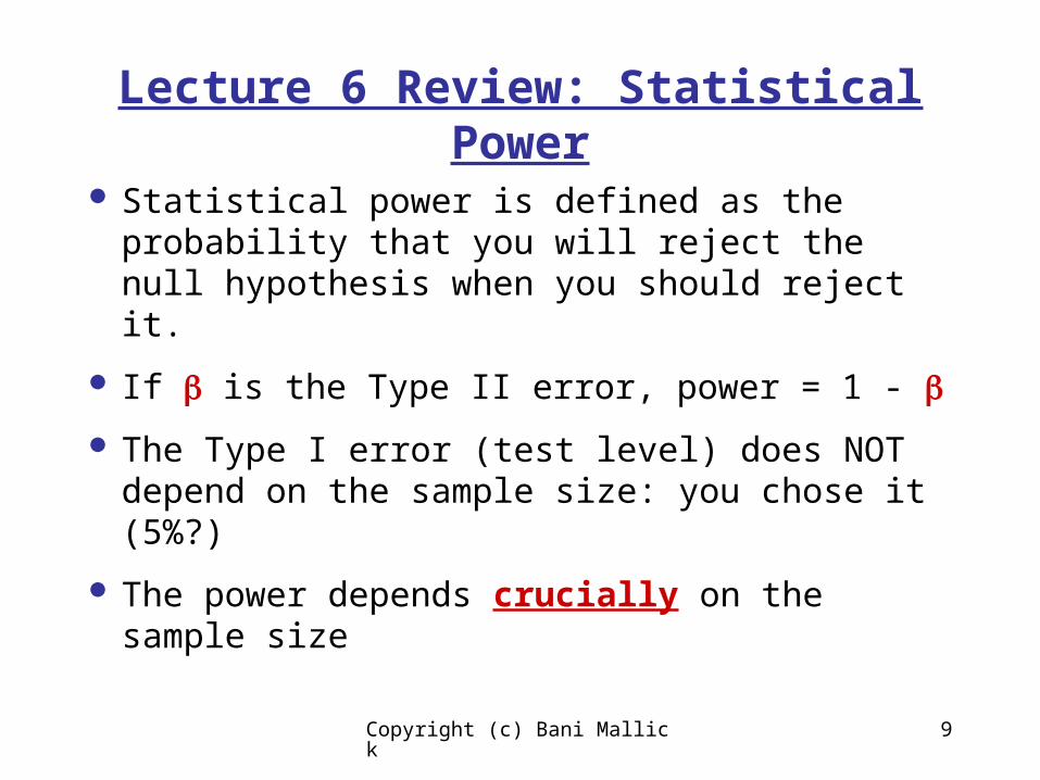
Lecture 6 Review: Statistical Power
Statistical power is defined as the probability that you will reject the null hypothesis when you should reject it.
If is the Type II error, power = 1 -
The Type I error (test level) does NOT depend on the sample size: you chose it (5%?)
The power depends crucially on the sample size
Copyright (c) Bani Mallick 10
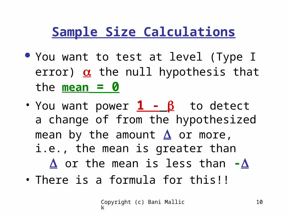
Sample Size Calculations
You want to test at level (Type I error) the null hypothesis that the mean = 0
• You want power 1 - to detect a change of from the hypothesized mean by the amount or more, i.e., the mean is greater than or the mean is less than -
• There is a formula for this!!
Copyright (c) Bani Mallick 11
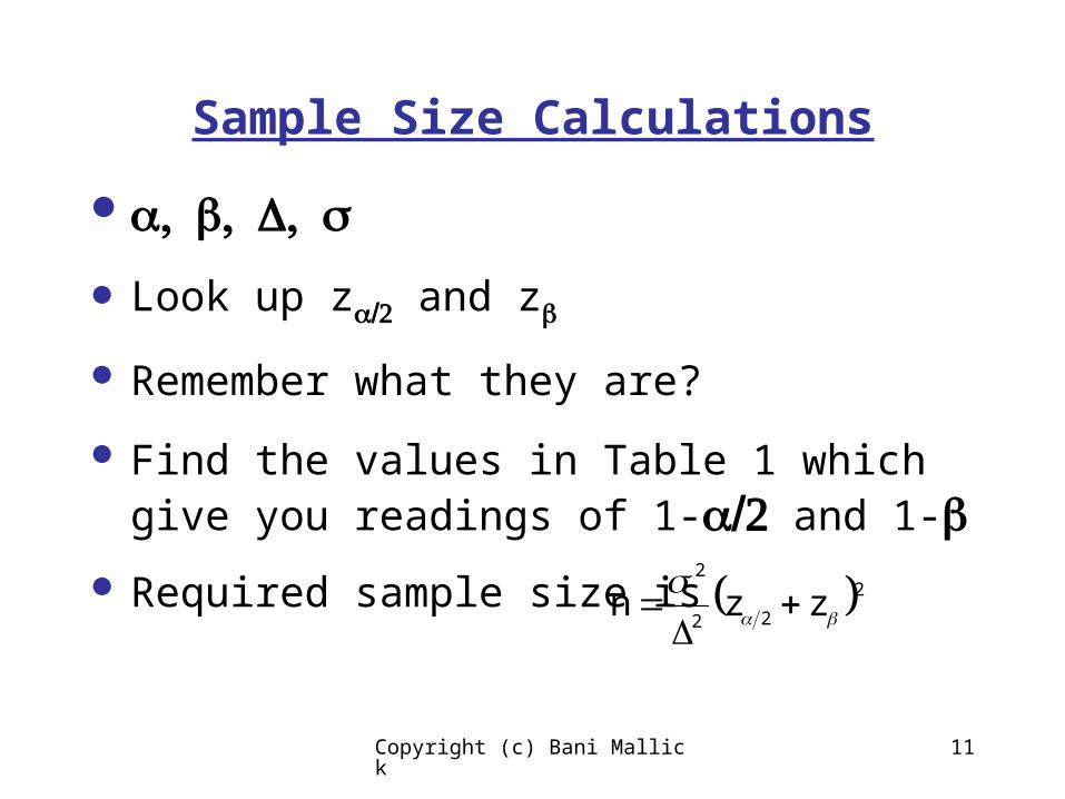
Sample Size Calculations
Look up z and z
Remember what they are?
Find the values in Table 1 which give you readings of 1-and 1-
Required sample size is 2
22
2
zzn
Copyright (c) Bani Mallick 12
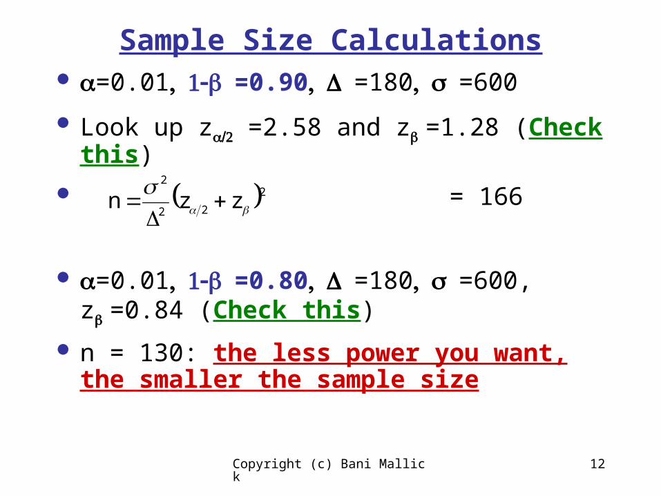
Sample Size Calculations =0.01=0.90=180=600
Look up z =2.58 and z=1.28 (Check this)
= 166
=0.01=0.80=180=600, z=0.84 (Check this)
n = 130: the less power you want, the smaller the sample size
2
22
2
zzn
Copyright (c) Bani Mallick 13
More on Sample Size Calculations
Most often, sample sizes are done by convention or convenience:
Your professor has used 5 rats/group before successfully
You have time only to interview 50 subjects in total
Copyright (c) Bani Mallick 14
More on Sample Size Calculations
More often, sample sizes are done by convention or convenience:
In this case, the sample size calculations can be used after a study if you find no statistically significant effect
You can then guess how large a study you would have needed to detect the effect you have just seen but which was not statistically significant
Copyright (c) Bani Mallick 15
Never Accept a Null Hypothesis
Suppose we use a 95% confidence interval, it includes zero. Why do I say: with 95% confidence, I cannot reject that the population mean is zero.
I never, ever say: I can therefore conclude that the population mean is zero.
Why is this? Are statisticians just weird? (maybe so, but not in this case)
Copyright (c) Bani Mallick 16
Never Accept a Null Hypothesis: Reason 1
Suppose we use a 95% confidence interval, it includes zero: [-3,6]. Why do I say: with 95% confidence, I cannot reject that the population mean is zero.
Remember the definition of a confidence interval: the chance is 95% that the true population mean is between -3 and 6: hence, the true population mean could be 5, and is not necessarily = 0.
Copyright (c) Bani Mallick 17
Never Accept a Null Hypothesis: Reason 2
Suppose we use a 95% confidence interval, it includes zero: [-3,6]. Why do I say: with 95% confidence, I cannot reject that the population mean is zero.
Potential for chicanery: if you want to accept the null hypothesis, how can you best insure it?
Copyright (c) Bani Mallick 18
Never Accept a Null Hypothesis: Reason 2
An example of chicanery: generic drugs
In the pharmaceutical industry, all the expense involves getting a drug approved by the FDA
After a drug goes off-patent, generic drugs can be marketed
The main regulation is that the generic must be shown to be “bioeqiuvalent” to the patent drug
Copyright (c) Bani Mallick 19
Never Accept a Null Hypothesis: Reason 2
The generic must be shown to be “bioeqiuvalent” to the patent drug
One way would be to run a study and do a statistical test to see whether the drugs have the same effects/actions: the null hypothesis is that the patent and generic are the same
The alternative is that they are not
If the null is rejected, the generic is rejected, and $$$ issues arise
Copyright (c) Bani Mallick 20
Never Accept a Null Hypothesis: Reason 2
Test to see whether the drugs have the same effects/actions: the null hypothesis is that the patent and generic are the same
If the null is rejected, the generic is rejected, and $$$ issues arise
If you pick a tiny sample size, there is no statistical power to reject the null hypothesis
Copyright (c) Bani Mallick 21
Never Accept a Null Hypothesis: Reason 2
If you pick a tiny sample size, there is no statistical power to reject the null hypothesis
The FDA is not stupid: they insist that the sample size be large enough that any medically important differences can be detected with 80% (1 - ) statistical power
Copyright (c) Bani Mallick 22
Never Accept a Null Hypothesis
p-values are not the probability that the null hypothesis is true.
For example, suppose you have a vested interest in not rejecting the null hypothesis.
Small sample sizes have the least power for detecting effects.
Small sample sizes imply large p-values.
Large p-values can be due to a lack of power, or a lack of an effect.
Copyright (c) Bani Mallick 23
Paired Comparisons: Count you Number of Populations!
The hormone assay data illustrate an important point.
Sometimes, we measure 2 variables on the same individuals
Reference Method and Test Method
There is only 1 population. How do we compare the two variables to see if they have the same mean?
Copyright (c) Bani Mallick 24
Paired Comparisons: Count you Number of Populations!
There is only 1 population. How do we compare the two variables to see if they have the same mean?
Answer (Ott & Longnecker, Chapter 6.4): do what we did and first compute the difference of the variables and make inference on this difference: now have 1 variable
In making inference, match the number of variables to the number of populations!
Copyright (c) Bani Mallick 25
Paired Comparisons in SPSS
SPSS has a nice routine way of doing a paired comparison analysis, providing confidence intervals and p-values
“Analyze”
“Compare Means”
“Paired Samples t-test”
Highlight the variables that are paired and select: use “options” to get other than 95% CI
Copyright (c) Bani Mallick 26
Paired Comparisons in SPSS
Demo using computer comes next
Copyright (c) Bani Mallick 27
Boxplots and Histograms for Paired data
For paired data, SPSS makes it easy to automatically get confidence intervals: it takes the difference of the paired variables for you
However, for boxplots, qq-plots, etc., you have to do this manually.
Here is how you can define a new variable, called “differen”, in the armspan data for males.
Copyright (c) Bani Mallick 28
Computing the Difference in Paired Comparisons
Click on “Transform”
Click on “Compute”
New window shows up, in “Target Variable” type in differen
Click on “Type & Label” and type in your label (Height - Armspan in Inches)
click on “Continue”
Copyright (c) Bani Mallick 29
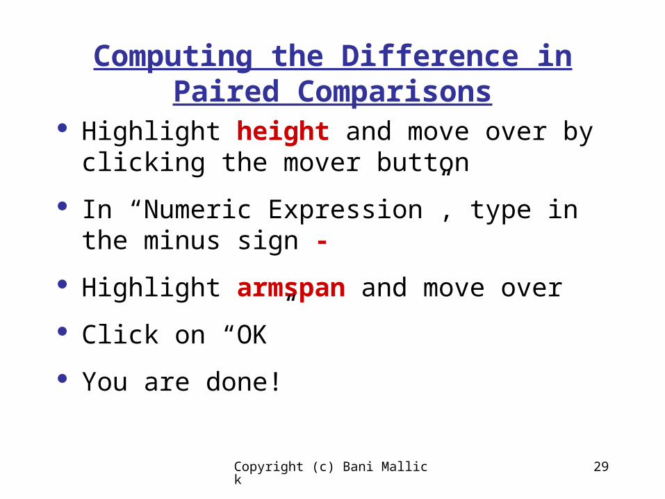
Computing the Difference in Paired Comparisons
Highlight height and move over by clicking the mover button
In “Numeric Expression”, type in the minus sign -
Highlight armspan and move over
Click on “OK”
You are done!
Copyright (c) Bani Mallick 30
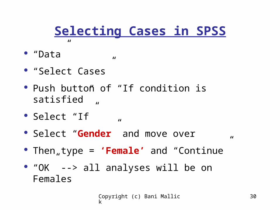
Selecting Cases in SPSS
“Data”
“Select Cases”
Push button of “If condition is satisfied”
Select “If”
Select “Gender” and move over
Then type = ‘Female’ and “Continue”
“OK” --> all analyses will be on Females
Copyright (c) Bani Mallick 31
Student’s t-Distribution
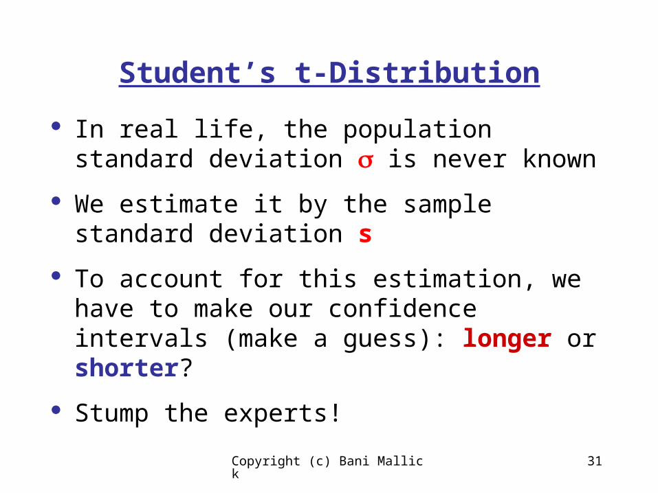
In real life, the population standard deviation is never known
We estimate it by the sample standard deviation s
To account for this estimation, we have to make our confidence intervals (make a guess): longer or shorter?
Stump the experts!
Copyright (c) Bani Mallick 32
Student’s t-distribution
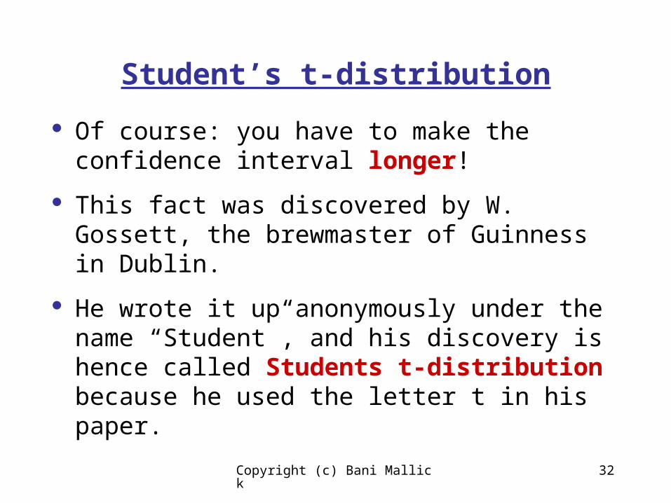
Of course: you have to make the confidence interval longer!
This fact was discovered by W. Gossett, the brewmaster of Guinness in Dublin.
He wrote it up anonymously under the name “Student”, and his discovery is hence called Students t-distribution because he used the letter t in his paper.
Copyright (c) Bani Mallick 33
Student’s t-Distribution
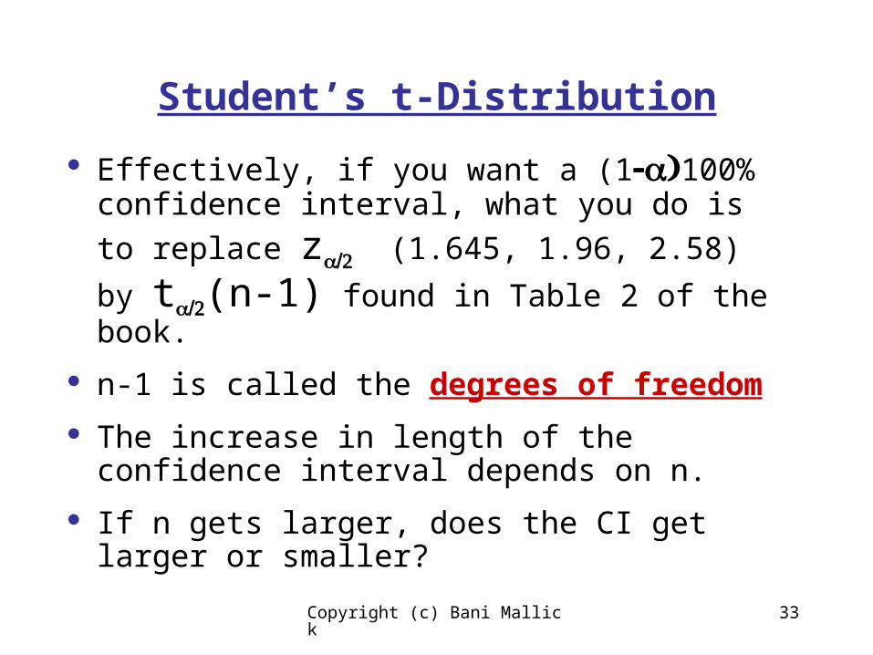
Effectively, if you want a (1100% confidence interval, what you do is to replace z (1.645, 1.96, 2.58) by
t(n-1) found in Table 2 of the book.
n-1 is called the degrees of freedom
The increase in length of the confidence interval depends on n.
If n gets larger, does the CI get larger or smaller?
Copyright (c) Bani Mallick 34
Student’s t-Distribution
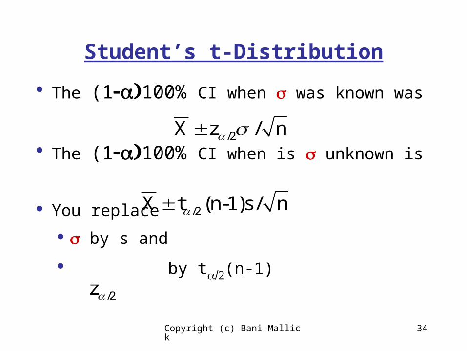
The (1100% CI when was known was
The (1100% CI when is unknown is
You replace
by s and
by t(n-1)
/2X z / n
/2X t (n-1)s / n
/2z
Copyright (c) Bani Mallick 35
Student’s t-Distribution
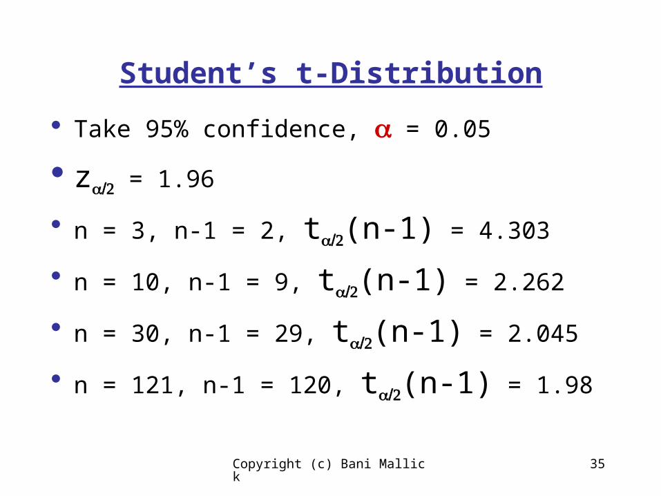
Take 95% confidence, = 0.05
z = 1.96
n = 3, n-1 = 2, t(n-1) = 4.303
n = 10, n-1 = 9, t(n-1) = 2.262
n = 30, n-1 = 29, t(n-1) = 2.045
n = 121, n-1 = 120, t(n-1) = 1.98
Copyright (c) Bani Mallick 36
Student’s t-Distribution
Luckily, SPSS is smart.
It automatically uses Student’s t-distribution in constructing confidence intervals and p-values!
So, all the output you will see in SPSS has this correction built in
Copyright (c) Bani Mallick 37
Student’s t-Distribution
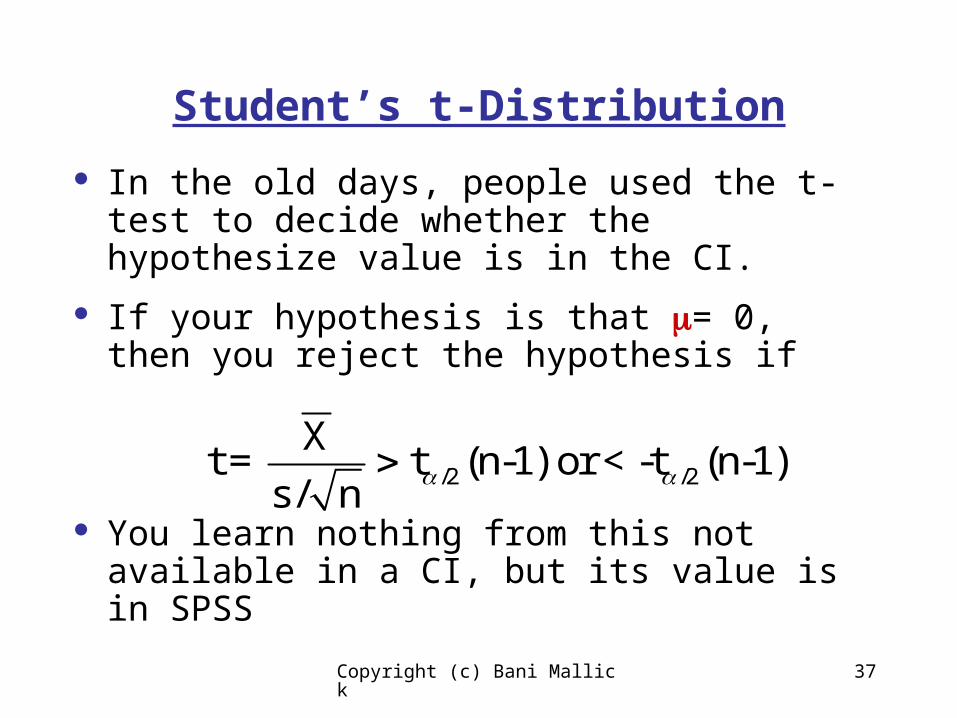
In the old days, people used the t-test to decide whether the hypothesize value is in the CI.
If your hypothesis is that = 0, then you reject the hypothesis if
You learn nothing from this not available in a CI, but its value is in SPSS
/2 /2
Xt = t (n-1) or < -t (n-1)
s / n
Copyright (c) Bani Mallick 38
WISH Numerical Illustration
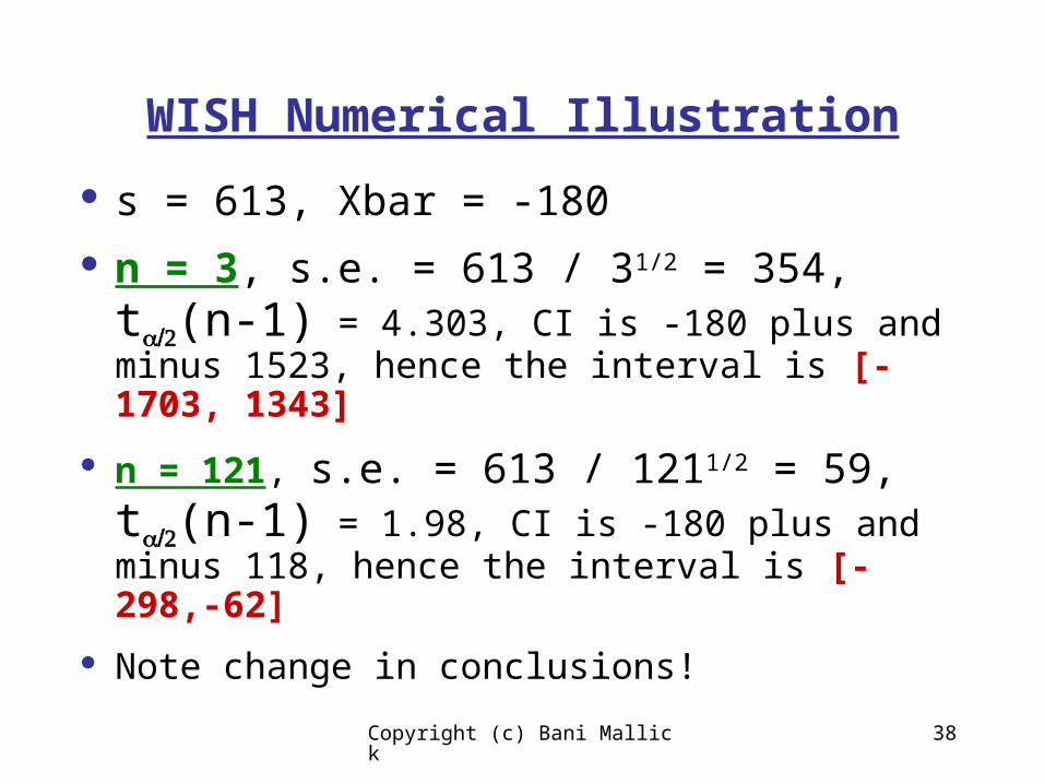
s = 613, Xbar = -180
n = 3, s.e. = 613 / 31/2 = 354, t(n-1) = 4.303, CI is -180 plus and minus 1523, hence the interval is [-1703, 1343]
n = 121, s.e. = 613 / 1211/2 = 59, t(n-1) = 1.98, CI is -180 plus and minus 118, hence the interval is [-298,-62]
Note change in conclusions!
Copyright (c) Bani Mallick 39
Armspan Data for Males
Outcome is height – armspan in inches
In SPSS, “Analyze”, “Descriptives”, “Explore” will get you to the right analysis
Illustrate how to do this in SPSS
Copyright (c) Bani Mallick 40
Armspan Data for Males
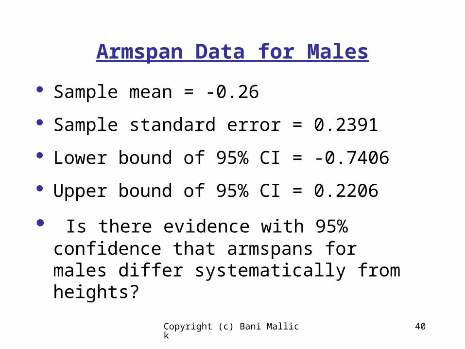
Sample mean = -0.26
Sample standard error = 0.2391
Lower bound of 95% CI = -0.7406
Upper bound of 95% CI = 0.2206
Is there evidence with 95% confidence that armspans for males differ systematically from heights?
Copyright (c) Bani Mallick 41
Armspan Data for Males
Might ask: what about with 90% confidence
Illustrate how to do this in SPSS

Copyright (c) Bani Mallick 42
Armspan Data for Males
Sample mean = -0.26
Sample standard error = 0.2391
Lower bound of 90% CI = -0.6609
Upper bound of 90% CI = 0.1409
Is there evidence with 90% confidence that armspans for males differ systematically from heights?
Copyright (c) Bani Mallick 43
Armspan Data for Males
SPSS will compute the p-value for you as well as confidence intervals.
For paired comparisons, “Analyze”, “Compare Means”, “Paired Sample”.
Highlight the paired variables.
It computes the difference of the first named variable in the list minus the second
Illustration in SPSS
Copyright (c) Bani Mallick 44
Armspan Data for Males
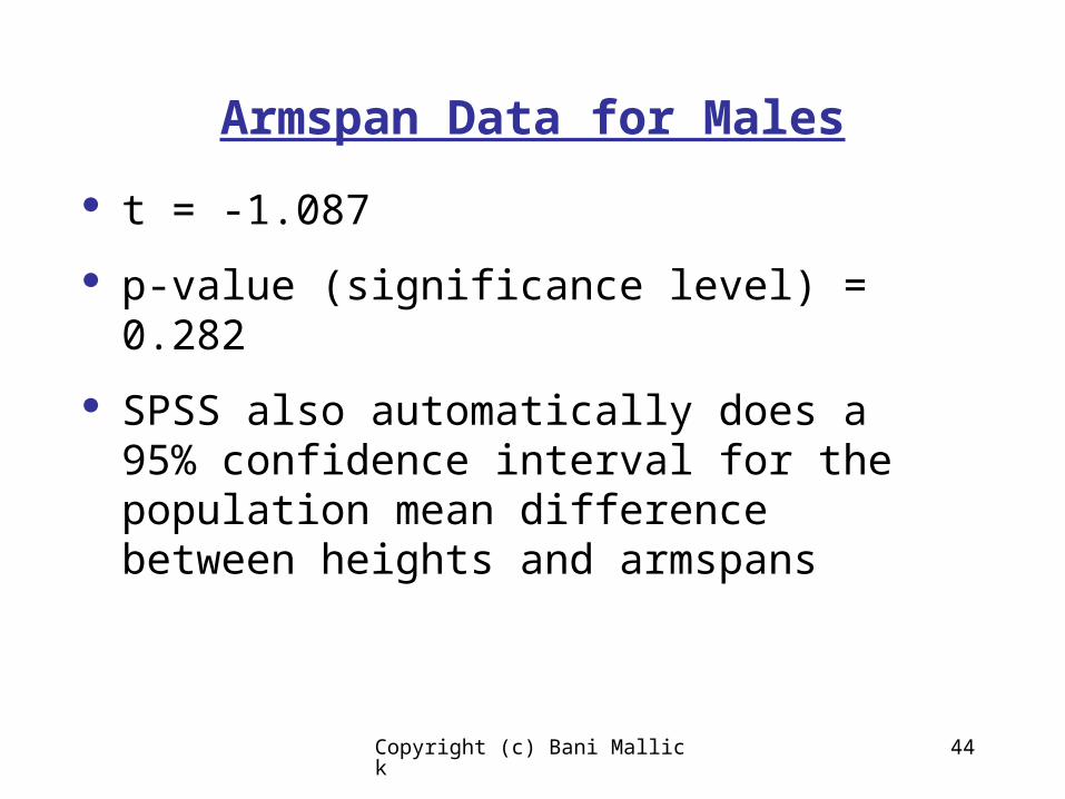
t = -1.087
p-value (significance level) = 0.282
SPSS also automatically does a 95% confidence interval for the population mean difference between heights and armspans