Copyright

by

Shane Suzanne Allua

2007

The Dissertation Committee for Shane Suzanne Allua certifies that this is the approved version of the following dissertation:

Evaluation of Single- and Multilevel

Factor Mixture Model Estimation

Committee:

Susan N. Beretvas, Supervisor

Laura M. Stapleton

Alexandra Loukas

Tim Keith

Keenan Pituch

Evaluation of Single- and Multilevel

Factor Mixture Model Estimation

by

Shane Suzanne Allua, B.S.; M.S.

Dissertation

Presented to the Faculty of the Graduate School of

the University of Texas at Austin

in Partial Fulfillment

of the Requirements

for the Degree of

Doctor of Philosophy

The University of Texas at Austin

May 2007

Dedication

Dedicated to my husband

Jonathan David Allua

v

Acknowledgments

I would first like to extend my appreciation to my advisors, Tasha Beretvas and Laura Stapleton for their support and guidance throughout my years in the doctoral program and most importantly, throughout the dissertation process. I would like to thank both of them for their dedication and flexibility which were pivotal to helping me succeed. I would also like to give thanks to the other committee members for their time and recommendations including Alexandra Loukas, Tim Keith, and Keenan Pituch.

To whom this is dedicated, my husband, for without him, this achievement would not be possible. I thank him for his understanding of the time commitment that this 5-year journey required and his devotion to my success. From his company in the late night hours to his surprise gifts of encouragement and most importantly for his love, I am forever grateful. I would also like to thank Archie for his unwavering loyalty, no matter how late the hour.

I would also like to thank my parents, Jan and Garnie McCormick, for being such an inspiration in my life. I thank them for instilling in me the drive to achieve and for leading by example. I give thanks to my brother, Nick, for the all of the visits to Starbucks that he made especially for me. The love and support of my family is truly a gift.

I would like to thank the Mplus Support Team for their programming assistance and expertise. Lastly, I would like to thank my manager and colleague at IBM, Don DeLuca and Paul Mullin, for their support and thoughtfulness.

vi

Evaluation of Single- and Multilevel

Factor Mixture Model Estimation

Publication No. _____________

Shane Suzanne Allua, Ph.D.

The University of Texas at Austin, 2007

Supervisor: Susan N. Beretvas

Confirmatory factor analysis (CFA) models test the plausibility of latent

constructs hypothesized to account for relations among observed variables. CFA models

can be used to model both hierarchical data structures as a result of cluster sampling

designs and investigate the plausibility of latent classes or unobserved classes of

individuals. Recent research has suggested preliminary evidence on the accuracy of

typical fit indices (AIC, BIC, aBIC, LMR aLRT) among various single-level latent class

models, multilevel latent class models that correct for biased standard error estimates as a

result of nested data, and growth mixture models (Clark & Muthén, 2007; Nylund et al.,

vii

2006, Tofighi & Enders, 2006). But few, if any, researchers have studied the accuracy of

the fit indices in multilevel factor mixture models. The purpose of this study was to

extend the literature in this less researched area and assess the performance of typical fit

indices used to compare factor mixture models. Class separation, intraclass correlation,

and between-cluster sample size were manipulated to emulate realistic typical research

conditions.

The proportion of times out of a possible 100 replications in which each of the

AIC, BIC, aBIC, and LMR aLRT led to selection of the correctly specified model among

other mis-specified models was recorded. Results for data generated to fit one-class

models indicated that the BIC and aBIC outperformed the AIC and the LMR aLRT was

nonsignificant nearly 100% of the time, supporting the correct one-class model.

Performance of all fit indices was, however, poor when data were generated to originate

from two-class models. The AIC and LMR aLRT tended to perform better than the BIC

and aBIC, although accuracy of all fit indices increased as a function of increasing class

separation and between-cluster sample size. Implications and recommendations regarding

optimal fit indices under various conditions are reported. It is hoped that the current

research has provided initial evidence of conditions in which the various fit indices are

more likely to model the correct number of latent classes in multilevel data.

viii

Table of Contents

Abstract......................................................................................................................... viList of Tables................................................................................................................. xList of Figures............................................................................................................... xiiChapter I: Introduction............................................................................................... 1Chapter II: Literature Review.................................................................................... 8

Confirmatory Factor Analysis............................................................................ 8Multiple Group Confirmatory Factor Analysis.................................................. 10

Measurement Invariance........................................................................ 10Latent Mean Comparison....................................................................... 13

Multilevel Confirmatory Factor Analysis.......................................................... 17Multilevel Modeling............................................................................... 19Configuration of the Multilevel Confirmatory Analysis Model............. 21Parameter and Standard Error Estimate Bias....................................... 26

Multilevel Multiple Group Confirmatory Factor Analysis – Between Groups................................................................................................................ 34

Multilevel Multiple Groups Confirmatory Factor Analysis – Within Clusters............................................................................................................... 37

Factor Mixture Models....................................................................................... 43Multilevel Factor Mixture Models..................................................................... 56Model Fit Indices............................................................................................... 58Statement of the Problem................................................................................... 66

Chapter III: Method.................................................................................................... 68Simulation Conditions........................................................................................ 68

Class Separation.................................................................................... 68ICC......................................................................................................... 70Sample Size............................................................................................. 70

Study Design Overview...................................................................................... 71Data Generation................................................................................................. 71Model Estimation............................................................................................... 75Data Analysis..................................................................................................... 80

Fit Indices............................................................................................... 81Parameter Estimate Bias........................................................................ 82Standard Error Estimate Bias................................................................ 83Convergence Rates................................................................................. 83

Chapter IV: Results..................................................................................................... 85Convergence Rates............................................................................................. 85Performance of the Fit Indices........................................................................... 89

AIC......................................................................................................... 89BIC......................................................................................................... 93aBIC....................................................................................................... 97LMR aLRT.............................................................................................. 100Comparison of Fit Indices...................................................................... 110

ix

Parameter and Standard Error Estimate Bias................................................ 124Parameter Estimate Bias........................................................................ 124Standard Error Estimate Bias................................................................ 130

Chapter V: Discussion................................................................................................. 138Convergence Problems...................................................................................... 138Performance of the Fit Indices........................................................................... 139Parameter and Standard Error Estimate Bias................................................ 142Implications and Recommendations................................................................... 143Limitations and Suggestions for Future Research............................................. 145General Conclusion............................................................................................ 147

References..................................................................................................................... 149Vita................................................................................................................................. 161

x

List of Tables

Table 1. Data Generation Characteristics....................................................... 73

Table 2. Data Generation Parameters............................................................. 75

Table 3. Percentage of Converged Solutions (Out of 100 Replications) as a Function of Generating Conditions.................................................. 87

Table 4. Percentage of Occurrences (Out of the Converged Solutions) the Correct Model was Selected whenα = 0 and ICC = .10.................. 112

Table 5. Percentage of Occurrences (Out of the Converged Solutions) the Correct Model was Selected whenα = 0 and ICC = .20.................. 113

Table 6. Percentage of Occurrences (Out of the Converged Solutions) the Correct Model was Selected whenα = .75 and ICC = .10............... 114

Table 7. Percentage of Occurrences (Out of the Converged Solutions) the Correct Model was Selected whenα = .75 and ICC = .20............... 115

Table 8. Percentage of Occurrences (Out of the Converged Solutions) the Correct Model was Selected whenα = 1.0 and ICC = .10............... 116

Table 9. Percentage of Occurrences (Out of the Converged Solutions) the Correct Model was Selected whenα = 1.0 and ICC = .20............... 117

Table 10. Percentage of Occurrences (Out of the Converged Solutions) the Correct Model was Selected whenα = 1.25 and ICC = .10............. 118

Table 11. Percentage of Occurrences (Out of the Converged Solutions) the Correct Model was Selected whenα = 1.25 and ICC = .20............. 119

Table 12. Percentage of Occurrences the LMR aLRT Led to Selection of the Correct One-class Model for α = 0.................................................. 120

Table 13. Percentage of Occurrences the LMR aLRT Led to Selection of the Correct One-class Model for α = .75............................................... 121

Table 14. Percentage of Occurrences the LMR aLRT Led to Selection of the Correct One-class Model for α = 1.0............................................... 122

xi

Table 15. Percentage of Occurrences the LMR aLRT Led to Selection of the Correct One-class Model for α = 1.25............................................. 123

Table 16. Relative Bias of Estimated Parameters for the Correct Model with 0=α for ICC = .10 and ICC = .20................................................. 126

Table 17. Relative Bias of Estimated Parameters for the Correct Model with 75.=α for ICC = .10 and ICC = .20.............................................. 127

Table 18. Relative Bias of Estimated Parameters for the Correct Model with 0.1=α for ICC = .10 and ICC = .20............................................... 128

Table 19. Relative Bias of Estimated Parameters for the Correct Model with 25.1=α for ICC = .10 and ICC = .20............................................. 129

Table 20. Relative Bias of Standard Error Estimates for the Correct Model with 0=α for ICC = .10 and ICC = .20......................................... 134

Table 21. Relative Bias of Standard Error Estimates for the Correct Model with 75.=α for ICC = .10 and ICC = .20...................................... 135

Table 22. Relative Bias of Standard Error Estimates for the Correct Model with 0.1=α for ICC = .10 and ICC = .20....................................... 136

Table 23. Relative Bias of Standard Error Estimates for the Correct Model with 25.1=α for ICC = .10 and ICC = .20..................................... 137

xii

List of Figures

Figure 1. Single Level Factor Mixture Model.................................................. 48

Figure 2. Single Level Factor Mixture Model with Covariate......................... 51

Figure 3. Single level Confirmatory Factor Analysis Model........................... 77

Figure 4a. Single Level Two-Class Factor Mixture Model............................... 78

Figure 4b. Single Level Three-Class Factor Mixture Model............................. 78

Figure 5. Multilevel Confirmatory Factor Analysis Model............................. 79

Figure 6a. Multilevel Two-Class Factor Mixture Model................................... 80

Figure 6b. Multilevel Three-Class Factor Mixture Model................................. 80

Figure 7. Percentage of Replications that the AIC Led to Selection of the Correct Model when ICC = .10........................................................ 91

Figure 8. Percentage of Replications that the AIC Led to Selection of the Correct Model when ICC = .20........................................................ 92

Figure 9. Percentage of Replications that the BIC Led to Selection of the Correct Model when ICC = .10........................................................ 95

Figure 10. Percentage of Replications that the BIC Led to Selection of the Correct Model when and ICC = .20.................................................. 96

Figure 11. Percentage of Replications that the aBIC Led to Selection of the Correct Model when ICC = .10........................................................ 98

Figure 12. Percentage of Replications that aBIC Led to Selection of the Correct Model when ICC = .20........................................................ 99

Figure 13. Percentage of Replications that the LMR aLRT Correctly Selected the k-class Multilevel Model when α = 0......................................... 101

Figure 14. Percentage of Replications that the LMR aLRT Correctly Selected the k-class Single Level Model when α = 0..................................... 102

xiii

Figure 15. Percentage of Replications that the LMR aLRT Correctly Selected the k-class Multilevel Model when α = .75...................................... 104

Figure 16. Percentage of Replications that the LMR aLRT Correctly Selected the k-class Multilevel Model when α = 1.0...................................... 105

Figure 17. Percentage of Replications that the LMR aLRT Correctly Selected the k-class Multilevel Model when α = 1.25.................................... 106

Figure 18. Percentage of Replications that the LMR aLRT Correctly Selected the k-class Single Level Model when α = .75.................................. 107

Figure 19. Percentage of Replications that the LMR aLRT Correctly Selected the k-class Single Level Model when α = 1.0.................................. 108

Figure 20. Percentage of Replications that the LMR aLRT Correctly Selected the k-class Single Level Model when α = 1.25................................ 109

1

Chapter I: Introduction

Behavioral science research is often characterized by the study of latent constructs

and group comparisons in which data may be part of a multistage sampling design. Group

comparison suggests the presence of subpopulations or groups of individuals within a

heterogeneous population. Subpopulations that are observed or are explicitly defined will

be referred to as groups. For instance, a sample may consist of males and females or

experimental and control groups. More recently, interest has extended beyond differences

in known groups leading to exploration of classes of individuals that are unknown.

Subpopulations that are unknown are called latent classes because group membership is

not observed. The latent classes are inferred from the data and can be used to discover

classes of individuals. Whether the heterogeneity in the population is observed or

unobserved, researchers are able to focus on the differences among the groups or classes.

The difference of interest can range from an observed variable to an unobserved variable

or latent construct.

Common analytic techniques such as analysis of variance (ANOVA) or structured

means modeling (SMM) that can be used to compare these groups are based on the

assumption of independent observations. Large-scale behavioral science research,

however, frequently takes advantage of multistage sampling which violates the

independence assumption. Cluster sampling, a form of multistage sampling, is a cost-

effective sampling technique that often yields very large sample sizes. Research

characterized by the comparison of observed groups and/or latent classes, together with a

2

clustered sampling design will be presented as a means to explore a series of single- and

multilevel confirmatory factor analysis (CFA) models.

CFA models are subsumed in a more general modeling framework known as

structural equation modeling (SEM; see, for example, Bollen, 1989, Kaplan, 2000). CFA

is also based on the assumption that the data consist of independent and identically

distributed observations. Clustered sampling designs result in data that are not only a

function of individual characteristics, but also of the variety of systems functioning at the

group level (Julian, 2001). For example, students can be compared or measured on a

variety of variables. However, varying characteristics of schools may differentially

impact the responses of students within schools. If the dependencies among the data are

not considered, incorrect conclusions can be drawn as a result of parameter and standard

error bias. Conceptual and methodological concerns that may result from nested data

have led to the development of multilevel modeling techniques (Heck & Thomas, 2000).

Multilevel regression models, also commonly referred to as hierarchical linear

models, have been featured in a variety of disciplines. Although these models account for

the nested nature of relationships, they do not allow researchers to examine covariance

structures or structural equation models (Farmer, 2000). Recognition of this limitation

has directed research interests to issues surrounding the use of multilevel CFA and SEM

techniques (Goldstein & McDonald, 1988; Heck, 2001; Heck & Thomas, 2000; Hox,

1995; McArdle & Hamagami, 1996; Muthén, 1991, 1994; Muthén & Satorra, 1989,

1995; Stapleton, 2002, 2005, 2006b).

3

Multilevel data structures that are modeled using nonhierarchical covariance

modeling (i.e. ignoring the data hierarchy) can lead to incorrect interpretations based on

biased results (Julian, 2001; Muthén & Satorra, 1995). In general, ignoring multilevel

data structures in nonhierarchical covariance modeling tends to lead to negatively biased

standard errors, an inflated model chi-square statistic, and in some cases, may result in

positively biased model parameters. CFA models have been extended to address the

potential consequences of hierarchical data structures. CFA multilevel modeling

techniques include covariance and/or mean structures which permit investigation of

measurement invariance across distinct groups as well as latent mean comparison across

the groups.

Similar to interest in differences across distinct groups, research on covariance

and/or means structures across latent classes is growing through the use of mixture

models. Factor mixture models (FMM) are a combination of the common factor model

(Thurstone, 1947) and classic latent class analysis (Lazarsfield & Henry, 1968). Lubke

and Muthén (2005) demonstrated the use of factor mixture models as a way to explore

factor structure in conjunction with unobserved population heterogeneity. The common

factor model is appropriate for data from a common single homogeneous population

while latent class models can be used to discover latent classes of participants. Latent

class models are used to explore subtypes of individuals within a sample where group

membership is unknown beforehand.

The taxonomy of single- and multilevel CFA models proposed in this study can

serve as a guide for researchers interested in latent mean comparison within

4

heterogeneous populations where data are both independent (single-level) and

nonindependent (multilevel). The single-level CFA model is appropriate when the goal of

the research is to support the plausibility of a factor structure within a homogeneous

population where observations are independent. Under a heterogeneous population, an

alternative model, the multiple indicator multiple cause model (MIMIC; Muthén, 1989),

tests differences in the factor mean among explicitly defined groups. MIMIC models

operate under the assumption of equivalent models across groups or measurement

invariance. Alternatively, a multiple group CFA offers the flexibility of an assumption of

partial measurement invariance. Multiple group CFA is more suitable for latent mean

comparison when full measurement invariance is not supported. If, however, the

researcher ignored the hierarchical data structure in either the MIMIC model or multiple

group CFA, the data dependency may not be modeled appropriately. Thus, it seems likely

that this could lead to spurious results as have been found in traditional multilevel

modeling (see, for example, Raudenbush & Bryk, 2002; Snijders & Bosker, 1994).

Rather than ignoring the multistage sampling design, the design can either be

accounted for statistically or modeled. If accounted for statistically (i.e., design-based

analysis), the nested data structure is considered a nuisance, but the model appropriately

attends to the consequences of the sampling design, resulting in more appropriate

estimates. If the data dependency is modeled (i.e., model-based analysis), the nested data

structure is of interest and relations among both the individual-level and cluster-level can

be explored. MIMIC and multiple group CFA can both be extended to model the data

hierarchy using a multilevel MIMIC model or multilevel multiple group CFA. Multilevel

5

models simultaneously model the within-cluster covariance matrix and the between-

cluster covariance matrix. Assuming invariance, multilevel MIMIC models can include a

grouping variable (i.e., covariate) at the within-cluster level and/or at the between-cluster

level. Alternatively, assuming a partially invariant model, a multilevel multiple group

CFA can be used to test latent means across explicitly defined groups at both the within-

and between-cluster level (Muthén, Khoo, & Gustafson, 1997; Stapleton, 2005).

Muthén et al. (1997) proposed a multilevel multiple group CFA which addresses

group comparison at the between-cluster level. For example, group comparison could be

investigated among public and private schools or intervention and control treatment

programs. Latent mean comparison must be among independent groups within a cluster.

In other words, the model proposed by Muthén et al. (1997) could not be used to compare

males and females nested within the same school. Stapleton (2005) proposed a multilevel

SMM which tests latent mean differences across different groups where the grouping

occurs within clusters. In her example, students (within-cluster level) are nested within

schools (between-cluster level) and children (e.g. students) from one-parent and two-

parent families are compared on an achievement measure. The modeling technique

proposed by Stapleton (2005) both models the data dependency due to clustering and

offers the flexibility of modeling partial measurement invariance across different groups

(i.e., males and females or one-parent and two-parent children) within clusters. Thus far,

the single and multilevel MIMIC models and the single- and multilevel multiple group

CFA models have focused on explicitly defined groups that are thought to partially

account for variability in the factor mean.

6

Above and beyond observed groupings, the possibility exists that there is

unobserved heterogeneity that can be used to help account for variability in factor means.

Here, unobserved clusters of individuals or latent classes of individuals are modeled to

account for factor variability. The unobserved classes can be examined to understand

typical characteristics of these classes which can then help in describing or naming the

latent classes. The addition of the latent class to the CFA model shifts focus to latent

mean comparison across the latent classes rather than across the observed groups as in

MIMIC or multiple group CFA models. The resultant model, a FMM, integrates the

common factor model and the latent class model. Similar to the multilevel MIMIC model

and multilevel multiple group CFA model used to account for data dependency among

observed groups, the multilevel factor mixture model (MLFMM) is appropriate for

exploring unobserved population heterogeneity when data are nested.

When modeling FMM or mixture models in general, the number of classes must

be pre-specified. In other words, the researcher must specify an hypothesized number of

classes that might be present in the data. The true number of classes, however, is

unknown. Therefore, researchers must rely on fit indices and various performance

indicators to identify the best fitting model (i.e., number of classes) among plausible

alternative models. Determining which model provides the best fit is, in part, a function

of the research question and should also incorporate theory as a decision factor. Even

with good model fit, however, plausibility of the model is only suggested and not

confirmed.

7

Common fit indices used in FMM include the Akaike Information Criteria (AIC;

Akaike, 1987), Bayesian Information Criteria (BIC, Schwartz, 1978), and the adjusted

BIC (aBIC; Sclove, 1987) where the lowest fit index value of the competing models

suggests the better fitting model. An additional fit index, the Lo-Mendell Rubin adjusted

likelihood ratio test (LMR aLRT; Lo, Mendell, & Rubin, 2001), is used to statistically

test the difference between a k-class model and k-1 class model. As mentioned, the

researcher should have some theoretical reasoning to support the number of classes.

Applied and methodological research using FMM has been minimal and even

more so for MLFMM. Applied researchers could benefit from methodological

researchers understanding of which model fit index most often correctly identifies the

true model and under what conditions the true model is more frequently selected.

Examination of the common fit indices can help uncover the conditions in which the

indices perform best or result in the highest percent of correct identification of the true

model.

In addition to studying the best performing fit index among alternative single- and

multilevel FMM, it is also of interest to study bias in parameter estimates and standard

error estimates. In other words, is bias present in parameter estimates and standard error

estimates for FMM as has been reported in other multilevel data structures when the data

hierarchy was modeled appropriately (Hox & Maas, 2001; Muthén & Satorra, 1995)? To

address the above questions, a series of single- and multilevel CFA models will be

investigated under a variety of conditions in which both data hierarchy and unobserved

population heterogeneity are specified correctly and incorrectly.

8

Chapter II: Review of Literature

A universal research question across various areas of the social sciences asks

whether there are mean differences among specific subpopulations. Analytic techniques

used to answer such research questions are, in part, determined by the nature and number

of dependent variables. Independent variables may also dictate choice of analysis;

however, the focus here will remain only on differences in the dependent variable. For

instance, a t-test can be used to test mean differences in one observed or manifest

dependent variable across two groups, such as males and females. Alternatively, a

multivariate analysis of variance (MANOVA) may be used when the analysis includes

more than one related manifest dependent variable. The dependent variable or variables

in the previous examples are observed and therefore measured variables. When the

dependent variable of interest is not observed and differences in a latent construct are of

primary interest, the t-test or MANOVA are no longer suitable analyses.

Analysis involving a construct or latent variable is generally referred to as

structural equation modeling (SEM). Single-level and multilevel modeling techniques

appropriate for testing latent mean differences among subpopulations will be addressed in

the review of literature. To help place each model in context, a substantive question of

interest relating to a measure of math ability precedes the description of each model.

Confirmatory Factor Analysis (CFA)

• Does a latent math ability factor explain the relations among a set of observed

variables?

9

Under the common factor model, it is assumed that the latent variable is

hypothesized to account for the relations among the measured variables of interest. Each

observed variable is assumed to be influenced, in part, by latent factors and unique

factors. CFA is one type of common factor model that is used to test for the plausibility

of a model. This type of model, consisting only of factors and the indicators that are used

to model the factors, is also called a measurement model (Kline, 1998). CFA, or the

measurement model, falls within the family of SEM which extends use of the CFA model

to include causal relations among factors. CFA models are used, among other things, to

quantify measurement error, validate theoretical models, and study differences in latent

means across various subpopulations of interest.

The common factor model for a p-dimensional vector of observed variables iy

may be expressed as

iii εληνy ++= (1)

ii ζαη += (2)

where ν is a p×1 vector of intercepts or means, λ is a p×1 vector of factor loadings, iη

is a N×1 vector of factor scores, and iε is a p×1 vector of residuals or the variability in

the observed variable that is not explained by the common factor. For a one-factor model,

α is a 11× vector (e.g. scalar) of the latent intercept or the average factor score, and iζ is

a N×1 vector of latent variable residuals. The single-level CFA (SLCFA) model assumes

that observations are independent and that the population is homogeneous or that all

observations in the population are similar. If it is reasonable to assume that

10

subpopulations are present, CFA can be extended to model the subpopulations. Joreskog

(1971) developed multiple group modeling which is a simultaneous modeling technique

used to test means and covariance structures in two or more predefined groups.

Multiple Group Confirmatory Factor Analysis

Research questions often address differences in latent means across members of

explicitly defined groups based on some observed variable. For instance, researchers

might be interested in comparing gender groups or cultural groups on some latent

variable such as achievement. Such research questions could be concerned with

measurement invariance or whether a set of indicators or items on a questionnaire

measure the same latent constructs across different groups (Kline, 1998). Multiple group

CFA is a commonly used procedure to test for measurement invariance and for G groups

gigigiggi εηλνy ++= (3)

giggi ζαη += (4)

where all parameters are as described in Equations 1 and 2, but can vary as a function of

group membership, indexed by g. If latent constructs are not measured similarly across

the groups, the validity of group comparison is questionable.

Measurement Invariance.

• Does the latent math ability factor similarly account for the relations among its

observed measures for both males and females?

Measurement invariance is typically assessed using a series of steps which have

been described in detail elsewhere (Bollen, 1989; Byrne, Shavelson, & Muthén, 1989;

Cheung & Rensvold, 1999; Vandenberg & Lance, 2000). Two types of invariance are

11

used to describe the common invariance hypotheses: measurement level and construct or

structural level invariance. Measurement invariance addresses relations between

measured variables and latent constructs whereas structural invariance addresses relations

among the latent variables themselves. If measurement invariance is not supported,

interpretation of latent mean differences is infeasible. Before comparing latent means, it

is reasonable to first determine if the latent construct has an equivalent meaning across

the groups.

To assess measurement invariance across the groups, various procedures have

been recommended. Vandenburg and Lance (2000) noted fourteen different methods of

assessing invariance that have been reported in the literature. Many of the methods

initially require a test of equality of covariance matrices followed by a test of configural

invariance (Horn & McArdle, 1992) or that the pattern of loadings and number of latent

variables are equivalent. Beyond configural invariance, Meredith (1993) has defined

measurement invariance using three sets of restrictions that must be imposed on the

model including invariance of factor loadings, intercepts, and residual variances.

Weak factorial invariance holds if factor loadings or the regressions of the

observed variables on the latent construct across groups are equal. Strong factorial

invariance holds if, in addition to equality of factor loadings, variable intercepts or means

can be assumed equal across groups. Strict factorial invariance holds if, in addition to

strong factorial invariance, residual or error variances are equal. Partial measurement

invariance is concluded if one or more of the restrictions are not supported (Byrne et al.,

1989). Although Meredith (1993) does not include invariance of factor variances in his

12

definition, Lubke and Dolan (2003) state that equality of factor variances is not a

requirement for measurement invariance. A lack of regard for factor variances by

Meredith (1993) would seem to violate the first step in measurement invariance as

concluded by Vandenburg and Lance (2000). Although various procedures for testing of

measurement invariance have been proposed (e.g., Alwin & Jackson, 1981; Drasgow &

Kanfer, 1985; Meredith & Millsap, 1992), Meredith’s (1993) definition appears widely

utilized and has been regarded as one of the most articulate and thorough to date

(DeShon, 2004).

Consider a single-factor model of achievement among males and females. If weak

factorial invariance is not supported, then males and females do not have an equal

increase or decrease in an observed variable for a one unit change in the achievement

construct, assuming the factor is on the same scale for both genders. In other words,

given the same increase in factor score across genders, the observed scores of say,

females, might increase more than that of males. If weak factorial invariance is

supported, but strong factorial invariance is not supported, one group scores consistently

higher or lower than the other independent of the scores on the factor. In other words, if

females have an advantage, that is, score higher, on a particular item, but the higher score

can not be attributed to a higher achievement score, then equality of intercepts across

gender is not supported. Differences in residual factor variances across the groups can be

due to differences in specific factor variance, random measurement error, or both.

Differences in specific factor variance or the reliable variance specific to the observed

variable suggests that for both genders, individual differences in observed scores are

13

differentially affected by the specific factors (Lubke & Muthén, 2005). Measurement

invariance is supported if a model that incorporates this set of three restrictions exhibits

good model fit. Group comparisons of latent means are, however, often regarded as

acceptable, if strong factorial invariance can be assumed (Little, 1997; Widaman &

Reise, 1997). One argument against satisfying this restriction is that unequal residual

variances suggest differences in reliability of the observed variables as opposed to a lack

of support for measurement invariance (Little, 1997; Lubke & Dolan, 2003).

Invariance is typically tested through the use of multiple group CFA. Here, the

primary interest is in testing measurement invariance across groups. Beyond testing

equality of covariances among the groups, testing differences in factor means is often a

secondary interest. Testing of latent means has also been referred to as structured means

modeling (SMM; Sörbom, 1974) and is an extension of multiple group CFA. Therefore,

these two analyses will be used interchangeably when discussing latent mean

comparison. Dependent upon support of measurement invariance, two modeling

techniques, multiple indicator multiple cause modeling (MIMIC, Muthén, 1989) and

SMM can be used to test latent mean differences among observed groups.

Latent Mean Comparison.

• Do males and females, on average differ in their level of math ability?

MIMIC and SMM are both used to test latent mean differences, but differ based

on the degree of measurement invariance that is assumed. MIMIC models include a

grouping variable as a covariate rather than specifying a model for each group (Muthén,

14

1989). Strict measurement invariance or equality of factor loadings, intercepts, and error

variances is a primary assumption of this model (Hancock, 1997).

Consider an example of a single latent construct η , indicated by p measured

variables, with a total of N observations where differences in the mean of η are to be

tested among G groups. The MIMIC model is defined such that

εηλy += y (5)

ζγXη += , (6)

where y is a p×N matrix of indicator variables, yλ is a p×1 vector of factor loadings, η is

a 1×N vector of factor scores, and ε is a p×N matrix of residuals, γ is a 1 × (G-1) vector

of regression coefficients, X is a (G-1) ×N matrix of dummy-coded group variables, and

ζ is a 1×N vector of residuals that represent the part of the latent variable (η ) that is not

explained by the grouping variable. To determine whether two groups (i.e., males and

females), on average, differed on their factor mean, the grouping variable or covariate, X,

would be a dummy coded variable represented by a vector with one regression coefficient

contained in γ (Muthén, 1989 ).

SMM provides an alternative to MIMIC modeling and does not require the

modeling of strict measurement invariance (Sörbom, 1974). In contrast to the regression

approach used in MIMIC models, SMM involves separating each group’s data so that all

model parameters can be modeled separately (Hancock, 1997). Assuming that the model

is still identified, equality constraints placed upon the models for the groups can be

15

released for any of the factor loadings and variances, residual variances, and intercepts.

SMM can be expressed as follows

εηλνy ++= y , (7)

where all matrices or vectors are similar to MIMIC modeling (see Equation 5 and 6) and

the additional parameter, ν is defined as a p×1 vector of intercepts. Factor scores can be

expressed as

ζαη += (8)

or as a function of α , the mean of the construct, and ζ , a 1×N vector of residuals. The

intercepts (ν ), factor loadings ( yΛ ), and residuals (ε ) can be held equal or freely

estimated across the G groups of interest. Prior to analyzing the means and intercepts,

however, some degree of measurement invariance is usually required (Chueng &

Rensvold, 1999; Vandenberg & Lance, 2000).

The ability to explore population heterogeneity and the assumption of

independent observations in both multiple group CFA and MIMIC models are of

particular focus in the current study. The degree to which a population consists of several

subpopulations is known as population heterogeneity. The source of population

heterogeneity can be observed or unobserved. Population heterogeneity is observed when

a measured variable such as gender or race accounts for differences in outcome variables.

Beyond using observed variables to study heterogeneity, unobserved

heterogeneity might be present. Here, the subpopulations are unobserved and can

therefore only be discovered from the estimation and interpretation of the model

parameters. The emergence of these subpopulations or latent classes can also be used to

16

address questions of invariance and/or differences in factor means across the latent

classes. In this case, the latent class could be used to partially account for variability in

factor loadings, intercepts, and residual variances which therefore addresses invariance

across the latent classes. Also, differences in factor means across the latent classes can be

tested. For instance, within the population under study, classes of “overachievers” and

“underachievers” might be present. However, these latent classes were likely not

apparent prior to the analysis.

Secondly, the use of single-level multiple group CFA and MIMIC models

assumes that observations are independent. However, data gathered using a multistage or

cluster sampling design violate this assumption. Violation of independent observations,

when modeled inappropriately, can lead to biased standard errors and inflated model chi-

square statistics (Julian, 2001; Muthén & Satorra, 1995). Biased parameter and standard

error estimates lead to incorrect conclusions regarding statistical significance and inflated

model chi-square statistics can result in inflated correct model rejection rates.

If it is reasonable to assume that the population under study is heterogeneous and

if the assumption of independent observations is violated, use of a single-level multiple

group CFA or MIMIC model may provide adequate fit, but alternative models may

provide a better fit and more accurate statistical inferences. CFA modeling alternatives

assuming a multistage sampling design will be discussed first, followed by modeling

alternatives with unknown population heterogeneity.

17

Multilevel Confirmatory Factor Analysis

• Assuming relations within- and between-clusters are of interest does a latent math

ability factor hypothesized within- and between-clusters explain the relations

among the observed variables?

Before multilevel model estimation techniques were available, single-level

analyses were used to analyze hierarchical data structures where either individuals or

clusters were the unit of analysis. Analytic techniques that are geared toward analyzing

hierarchical data structures have been called hierarchical or multilevel models (e.g.,

Raudenbush & Bryk, 2002). Use of structural equation modeling for hierarchical data

structures has been discussed by several researchers (Goldstein & McDonald, 1988;

McDonald & Goldstein, 1989; Muthén, 1989, 1994; Muthén & Satorra, 1995). Multilevel

models are appropriate for data that have a hierarchical or nested data structure where

students are nested within schools, patients within clinics, individuals within families,

etc.

As has been mentioned by various researchers (Bryk & Raudenbush, 1992; Diez-

Roux, 2000; Li, Duncan, Duncan, Harmer, & Acock, 1997; Reise, Ventura, Nuechterlein,

& Kim, 2005; Toyland & DeAyala, 2005), in the behavioral and social sciences,

hierarchical data structures are common yet often modeled inappropriately. Researchers

should recognize the potential impact of multistage sampling designs on model

parameters, standard errors, and model fit, and incorporate modeling techniques that are

designed to account for this bias.

18

Various analysis options exist for multistage sampling designs: pooled-within

cluster covariance matrix modeling, multilevel covariance structure modeling or

multilevel confirmatory factor analysis (MLCFA). Within multilevel modeling, data

dependency can be modeled using a model-based approach or using a design-based

approach (Muthén & Satorra, 1995). The model-based approach models relations both

within- and between-clusters whereas a design-based approach, among other methods,

statistically accounts for the clustering using sandwich estimators (see, e.g. Muthén &

Satorra, 1995; Stapleton, 2006a, 2006b). As opposed to modeling the relations between-

clusters, the sandwich estimator approach assumes any relations between-clusters are a

nuisance and appropriately accounts for the clustering statistically. The alternative

methods result in more accurate standard error estimates as opposed to a nonhierarchical

analysis when the nesting of the data is ignored.

Research questions that only address relations within a cluster can be modeled

using the pooled-within clusters covariance matrix. If only the pooled-within clusters

covariance matrix is analyzed, relations at the between-cluster level are ignored (Hox,

2002). Modeling the pooled-within clusters covariance matrix, as opposed to the total

covariance matrix, is one way of handling bias as a result of cluster sampling (Muthén,

1989). When the research question focuses on exploration of relations at both the within-

cluster and between-cluster level, analysis of only the pooled-within cluster covariance

matrix is inadequate. Rather, multilevel models that simultaneously model the within-

and between-cluster covariance matrices are necessary.

19

Multilevel modeling provides two advantages over the pooled within-cluster

covariance matrix. First, the variability that exists between clusters in the measured

variables can be estimated and then modeled. Secondly, sample size is based on the

pooled-within covariance matrix (N-C) in addition to the between-cluster covariance

matrix (C) where N is the total sample size and C is the number of clusters. The

additional information provided by the between-cluster covariance matrix helps increase

power to identify the correct model and nonzero relationships over analyses involving

only the within-cluster covariance matrix (Stapleton, 2006b). Investigation of both

within- and between-cluster relations can help uncover new substantive theories or can

now finally support substantive theories that before were not possible because of the

limitations of a single-level analysis (Heck, 2001). It is the multilevel model-based

techniques that are of interest in the current study and will be explored in further detail.

The multilevel formulation of the CFA model offers examination of construct

validity within- and between-clusters, quantification of measurement error both within-

and between-clusters, and latent mean comparison across the clusters. It is not uncommon

for different factor structures to emerge at the within- and between-cluster level (see, for

example Hox, 2002; Muthén, Khoo, & Gustafson, 1997). If within- and between-cluster

factor models differ, the degree to which they differ in factor structure, factor loading

patterns, relationships among factors, and measurement quality, for instance, can be

examined.

Multilevel Modeling. The assumption of independence among the observations in

conventional or SLCFA models suggests that the individuals within clusters do not share

20

common characteristics or perceptions. Ignoring this dependence can introduce

potentially important biases into the analysis. Prior to undertaking a multilevel analysis,

the design effect which includes the degree of between-cluster variability or the intraclass

correlation (ICC) should be considered. The ICC describes the amount of variance in the

observed variables that can be attributed to differences at the between-cluster level as

compared to the within-cluster level. In other words, the ICC is the ratio of the between-

cluster variance to the total variance and is defined as

)/( 222WBBICC σσσρ += (9)

(Muthén, 1989, 1994). ICC values around .20 have been described as both low (Hox &

Maas, 2001) and moderately-sized (Kreft & de Leeuw, 1998), and values around .30 as

high (Hox & Maas, 2001). Hox and Maas (2001) suggest that most ICC values in

education research are below. 20; however, Muthén (1997) has found ICC values for

intact classrooms to range from .3 to .4 for mathematics achievement.

In the presence of nested data, the design effect is a measure of the amount of bias

in the sampling variance of the mean. The design effect is approximately equal to 1+(n.-

1)*ICC where n. is the average cluster size (Kish, 1965). The design effect is thus

impacted by both the ICC and sample size and indicates the degree of underestimation of

the sampling variance if the clustering is ignored. The larger the within-cluster sample

size, the larger the impact on standard error estimation bias. Design effects less than two

typically result is unbiased estimates and do not necessarily indicate a need for a

multilevel analysis (Muthén & Satorra, 1995).

21

When modeling nested or hierarchical data structures, sample size must be

considered at both the within-cluster and between-cluster level. In a hierarchical

regression context, the ‘30/30’ rule (Kreft, 1996) suggests a sample consisting of no

fewer than 30 clusters each containing at least 30 individuals or observations per cluster.

Maas and Hox (2004) concluded that the 30/30 rule is valid for the estimation of fixed

parameters and random parameters at the individual level, but not for estimation of

random parameters at the cluster level. Estimation of random parameters in hierarchical

regression and their standard errors require a large number of clusters (C > 100) for

accurate estimates (Busing, 1993; Van der Leeden & Busing, 1994). Similar to the

recommendation for multilevel regression models, Hox and Maas (2001) caution against

using MLCFA when the number of groups is less than 100, especially if the ICC is low,

or under .25.

If the design effect is >2 and/or the ICC > 0, multilevel modeling may be a more

appropriate analysis to account for the nonindependence among observations and the

biases that may result. The configuration of the model-based MLCFA will be discussed

followed by discussion of parameter and standard error estimation bias reported in

MLCFA models under various conditions.

Configuration of the Multilevel Confirmatory Factor Analysis Model. Consider an

observed variable, y1, as being composed of variability from two parts: variability due to

differences among clusters, and variability due to differences among individuals.

Therefore, the variance in y1, 21yσ , consists of some function of the between-cluster

variability ( 2Bσ ) and some function of the within-cluster variability ( 2

Wσ ). The

22

partitioning of the variability into within- and between-cluster variance has been referred

to as disaggregated modeling (Muthén & Satorra, 1995) or a model-based analysis.

Instead of a single observed variable, consider a single-factor model indicated by p

observed variables where individuals are nested within C clusters. Subscripts c and i will

be used for clusters (i.e., schools) and individual observations (i.e., students),

respectively, and B and W refer to between-cluster and within-cluster components. To

clarify the within- and between-cluster level components, a one-factor MLCFA can be

expressed as

WciBcWciWBcBccBci εεηληλνy ++++= (10)

BcBBc ζαη += (11)

WciWci ζη = . (12)

Here, Bcν is the vector of intercepts, Bcλ is a vector of factor loadings, Bcε a vector of

residuals, Bcη is a random factor that models school effects, Bα is the intercept of Bcη or

the average factor score across all clusters, and Bcζ represents random variance in the

factor, all of which are a function of the between-cluster level or cluster variability.

Similarly, Wcλ represents a vector of factor loadings, Wciε a vector of residuals, wciη is a

random factor that varies across the within-cluster level units (i.e., students), and Wciζ

represents random variance of the factor at the within-cluster level, all of which are a

function of the within-cluster level or individual variability. Notice that Wα is not

estimated because the factor mean within-clusters is assumed zero (Muthén, 1994). The

parsing of the variance results in independence among the within-cluster covariance

23

matrix and between-cluster covariance matrix and thus, Bcη and Wciη are independent, as

are random coefficients in regression models (Hox, 1995; Muthén & Satorra, 1989). To

test differences in the factor mean across clusters (here, schools) in a conventional

multiple group modeling context, C−1 factor means would be estimated for the C

schools. Typically, one factor mean is set equal to 0; therefore, C-1 factor means are

estimated. In a multilevel context, however, schools are viewed as randomly selected

from some larger population of schools suggesting that the factor mean should be

specified as a random effect.

Multilevel modeling incorporates the random effects specification of varying

factor means where the total factor variance [ )( ciVar η ] can be separated into two parts:

variance within-clusters and variance between-clusters:

WBTciVar Ψ+Ψ=Ψ=)(η (13)

(Muthén, 1994). The amount of between-cluster factor variability relative to the total

factor variability can also be estimated. At the factor level, BΨ describes the magnitude

of nonindependence or the variability as a result of clustering. Muthén (1991) discusses

the latent variable equivalent of the ICC as the ratio of

)/( WBBICC Ψ+ΨΨ=ρ (14)

Thus, the amount of factor variability due to variation between clusters is calculated as

the ratio of factor variance between-clusters to the total factor variance.

For a p×p covariance matrix of observed variables, the disaggregation of the

population covariance matrix (Σ ) is defined as WBT ΣΣΣ += where TΣ is the total

24

aggregated population covariance matrix, BΣ is the between-clusters population

covariance matrix, and WΣ is the within-cluster population covariance matrix. Similarly,

the sample covariance matrix (S) can be defined as ST = SB + SW where ST is the total

aggregated sample covariance matrix, SB is the between-cluster level sample covariance

matrix, and SW is the within-cluster level sample covariance matrix (Muthén, 1994).

To allow the sample within- and between-cluster covariance matrices to be

modeled simultaneously, Muthén (1994) and Muthén and Satorra (1995) proposed a

multiple group modeling technique. Consider the three customary sample covariance

matrices, ST, SPW, and SB,

( ) ∑∑= =

− ′−−−=C

c

n

iciciT

c

yyyyN1 1

1 ))((1S (15)

( ) ∑∑= =

− ′−−−=C

c

n

iccicciWP

c

yyyyCN1 1

1 ))((S (16)

( ) ∑=

− ′−−−=C

ccccB yyyynC

1

1 ))((1S (17)

where grand mean responses are represented by a vector, y , and nc is the sample size per

cluster. For C balanced or equally sized clusters, the pooled-within matrix, SPW, is a

consistent and unbiased maximum likelihood estimator of WΣ ( WPWE ΣS =][ ) (Muthén,

1994). The sample between-clusters covariance matrix (SB), however, is not a consistent

and unbiased estimator of BΣ . Rather, SB, also referred to as a scaled-between matrix

(Hox, 2002), is a consistent and unbiased maximum likelihood estimator of BW n ΣΣ .+

25

( BWB nE ΣΣS .][ += ), where n. reflects the common cluster size across clusters (Muthén,

1994) and is defined as

n. = )1(

1

22

−

−∑=

CN

nNC

cc

. (18)

Thus, within- and between-cluster variance/covariance information is contained in SB.

Using a multiple group CFA, Muthén (1989, 1990) showed that MLCFA

parameters can be estimated using full information maximum likelihood (FIML)

estimation when the following fit function is minimized in a balanced design:

FML = +−−+++ − }||log]ˆ.ˆ[|ˆ.ˆ|{log 1 pntrnC BBWBW SΣΣΣΣ

}||log]ˆ[|ˆ|){log( 1 ptrCN PWWW −−+− − SΣΣ . (19)

Here, WΣ and BΣ represent the estimated or model-implied within- and between-cluster

covariance matrices, n. is the common group size and where the same WΣ holds for all

clusters in the population. The fit function is used to locate the best solution that results in

the smallest difference between the model-implied and the sample covariance matrices

(Heck, 2001). If interest lies only at the within-cluster level, using SPW to test the model

will directly estimate WΣ . For BΣ , a model for both, SPW, the within-clusters covariance

matrix and SB, the between-clusters covariance matrix, must be specified (Hox, 2002).

Prior to the advancements in various software programs which increased the ease of

specifying multilevel models, previous software programs could be “tricked” into

estimating multilevel models. In other words, from a multiple group perspective, two

“groups” are specified. The first “group” models the within-cluster variability (SPW)

26

whereas the second “group” models SB, which is a function of both the within-cluster and

between-cluster variability. The same WΣ matrix must be estimated for both “groups”.

Multilevel modeling is one option that can be used to account for

nonindependence of data as a result of clustered sampling designs. Multilevel modeling is

valuable in that theoretical models can be modeled both within- and between-clusters.

Researchers should be aware of the consequences of not correctly modeling the data

hierarchy. Not only do researchers miss the opportunity to explore between-cluster

relations if the data hierarchy is ignored, but researches are likely to conclude misleading

significant relations among variables due to the bias in the standard error estimates. In

addition to evaluating bias when the data hierarchy is ignored, bias has also been studied

when the data hierarchy is modeled appropriately.

Parameter and Standard Error Estimate Bias

One way to identify the impact of nonhierarchical analysis with hierarchical data

is to study bias of the parameter and standard error estimates. Muthén and Satorra (1995)

were one of the first to study parameter and standard error estimate bias of both a

correctly specified and incorrectly specified CFA model using a simulation design.

Muthén and Satorra (1995) explored the chi-square statistic and parameter and standard

error estimate bias under varying conditions of ICC (.05, .10, .20) and sample size at the

within-cluster level (i.e., cluster size; 7, 15, 30, 60) where the between-cluster sample

size or number of clusters was held constant at 200 clusters. To evaluate bias as a result

of nonhierarchical analysis of multilevel data, the true hierarchical structure of the

multilevel, 10-item, 2-factor CFA model was both ignored and modeled correctly using a

27

model-based and a design-based approach. When the data hierarchy was ignored,

maximum likelihood (ML) estimation was used. ML estimation under robust normal

theory analysis (i.e., sandwich estimator) and full information maximum likelihood

(FIML) were used when the data hierarchy was analyzed with a design-based and model-

based approach, respectively.

Under ML estimation assuming a mis-specified conventional SLCFA model, ICC

values and cluster size appear to be positively related to the distortion of the chi-square

where distortion of the chi-square was greatest at the highest level of ICC and cluster

size. The smallest ICC value (ICC= .05) combined with a cluster size of 60, however,

still produced severe distortion with a rate of 20.4, which is far beyond the 95%

prediction interval of 3.6 to 6.4. As a cluster size of 60 is often exceeded in large-scale

survey research (Muthén & Satorra, 1995), the importance of appropriately accounting

for the dependency even under low ICC values is evident. Using the robust normal theory

analysis however, distortion of the chi-square was eliminated and appeared to

overcorrect, slightly falling below the lower end of the prediction interval.

Similar to the distortion of the chi-square under a mis-specified SLCFA model,

bias of standard error estimates for factor loadings, error variances, and factor variance

was greatest for the highest ICC value and largest cluster size. Specifically, for all cluster

sizes under an ICC value of .20, standard error estimate bias for all parameters ranged

from -9% to -45%. Negative standard error bias resulted in nearly all conditions;

however bias appeared to be greater for residual variance estimates as compared to factor

loadings and factor variance estimates in all ICC and cluster size conditions. Bias of the

28

standard error estimates for all parameters decreased to minimal bias levels in most

conditions, however, under the robust normal theory analysis. The inaccuracy of the chi-

square and magnitude of bias in the standard error estimates for the mis-specified SLCFA

coupled with the improvement of the chi-square distortion and standard error estimate

bias for the robust normal theory analysis supports the recommendation to appropriately

model the nonindependence of the data.

Similar to Muthén and Satorra (1995), Julian (2001) studied the consequences of

ignoring the multilevel data structure on four sets of parameter estimates (factor loadings,

variances, and covariances, and error variances), standard error estimates for the four sets

of parameters, and the chi-square statistic. Multilevel data were generated; however,

single-level, four-factor CFA models were fit to the total covariance matrix using

maximum likelihood estimation. Extending the work of Muthén and Satorra (1995),

Julian’s (2001) simulation conditions also incorporated varied ICC levels [low (.05),

moderate (.15), and high (.45)], but expanded the sample size condition configuration

which was presented as a ratio of number of groups (NG) to group size (GS) ratio:100/5,

50/10, 25/20, and 10/50. In addition to the ICC and sample size configuration conditions,

model complexity was varied to include three multilevel model structures. At the within-

cluster level, the three multilevel model structures consisted of a 4-factor model (4F) with

each factor indicated by 4 items. Model variability was presented at the between-cluster

level and included a 4-factor model indicated by 4 items each (4F), a 2-factor model (2F)

indicated by 8 items each, and a 5-factor model (5F) with 4-factors indicated by 3 items

29

each and 1-factor indicated by 4 items. Therefore, the following three multilevel model

structures were generated: 4F-4F, 4F-2F, and 4F-5F.

Across all three model structures, although the low ICC condition resulted in the

chi-square statistic falling within or near the 95% confidence interval for the expected

rejection frequency, the values were still inflated to some extent and rejected too often for

all sample size configuration conditions. Inflation of the chi-square statistic and incorrect

rejection increased with increasing ICC values and as the number of groups/group size

ratio decreased.

Only under high ICC and group membership conditions of 25/20 and 10/50 did

positive factor loading estimation bias exceed 5%. Under low ICC conditions, bias of

factor variance and covariance estimates, and error variance estimates was negligible, but

bias increased considerably under moderate and high ICC conditions. Specifically, bias

of factor variance and covariance estimates, and error variance estimates ranged from

13% to 24% under the moderate ICC condition and from 63% to 109% under the high

ICC condition (Julian, 2001). Unlike the chi-square statistic, parameter estimate bias was

relatively unaffected by sample size configuration under low and moderate ICC values.

Under high ICC conditions, bias tended to decrease among decreasing ratios of number

of groups/group size. Consistent with the chi-square statistic, however, model structure

had little impact on parameter estimate bias.

Across nearly all conditions, models, and parameters, the standard error estimate

bias was negative and largely impacted by ICC values. That is, bias was minimal (0-8%)

under conditions of low ICC, but ranged from 5%-36% under the moderate ICC

30

condition, and from 26%-76% under conditions of high ICC. Similar to bias in the chi-

square statistic, sample size configuration had a large influence on size of bias where bias

increased as the group number/group size ratio decreased. Like bias in the chi-square

statistic and parameters, standard error estimate bias was minimally influenced by model

structure.

Nonhierarchical analysis of multilevel data then, appears to have a more critical

impact on the chi-square and standard error estimates at higher ICC values and when

within-cluster sizes are larger or when the number of groups/group size ratio decreases.

Moderate ICC values and in some cases low ICC values, however, tend to also produce

bias. The results emphasize the need to appropriately model the data dependency.

Muthén and Satorra (1995) and Julian (2001) established conditions under which

bias likely occurs under nonhierarchical analysis with multilevel data. In addition to mis-

specifying a SLCFA, Muthén and Satorra (1995) assessed bias in the chi-square statistic,

parameter estimates, and standard error estimates when the data hierarchy was

appropriately modeled using FIML under the same conditions as previously discussed

(ICC=.05, .10, .20; sample size at the within-cluster level =7, 15, 30, 60).

When the model was appropriately specified as a MLCFA, chi-square

performance was excellent across all conditions. Minimal parameter and standard error

estimate bias (< 5%) for within-cluster factor loadings and variances and within-cluster

residual variances were reported. Between-cluster parameter estimates resulted in

positive bias for the factor loadings (0-6%) and factor variances (2-11%), while

consistently negative (1-3%) for residual variances. Overall, however, parameter estimate

31

bias at the between-cluster was negligible (Muthén & Satorra, 1995). Conversely,

between-cluster standard error estimate bias was consistently negative across all

parameters’ standard errors and nonnegligible (1-18%), especially for lower ICC values.

ICC values of .20 in conjunction with larger cluster sizes resulted in minimal bias. In

general, Muthén and Satorra (1995) concluded that the correctly specified MLCFA model

resulted in minimal parameter and standard error estimate bias, especially under larger

sample sizes and higher ICC values and noted its utility for modeling nested data.

Whereas Muthén and Satorra (1995) evaluated the chi-square statistic and

parameter and standard error estimation bias using FIML, Hox and Maas (2001)

examined the accuracy of the chi-square model test, parameter estimates, and standard

error estimates, using the pseudo-balanced estimation technique. For a six-item, two-

factor within-cluster model and a one-factor between-cluster model, the following

simulation conditions were tested: (a) balanced vs. unbalanced clusters; (b) number of

clusters (NC = 50, 100, 200); (c) average cluster size (CS = 10, 20, 50); and (d) low vs.

high ICC values where between-cluster factor variance was .25 or .5 giving an average

ICC of .20 (low) and .33 (high).

Under a balanced condition, the pseudo-balanced estimation produces a FIML

solution creating unbiased parameter estimates with asymptotically correct standard

errors (Hox & Maas, 2001). Under unbalanced conditions, the pseudo-balanced

estimation is unbiased and consistent, but does not consider all of the variability in the

data. Thus, unbiased parameter estimates were expected, but the extent of the variability

in the standard errors and chi-squares from their nominal values was unknown.

32

Chi-square bias was measured as the deviation from the expected value which is

equal to the degrees of freedom and a value of 18 for the relevant model. The overall

mean of the chi-square was 18.8 resulting in a 4.0% bias. Under a true model, it was

expected that only 5% of the chi-square tests would be rejected assuming a 5% alpha-

level (Hox & Maas, 2001). Overall, 6.9% of the models were rejected under a 5%

significance level. Balance of the clusters and ICC values were the only conditions to

impact size of the chi-square and rejection rates. Balanced conditions resulted in less bias

(-0.5%) and more accurate rejections (4.9%) as opposed to unbalanced conditions, with

8.6% bias and rejection at 8.9%. The positive relationship between ICC and bias

emphasizes the importance of modeling the data dependence rather than ignoring it,

especially under conditions of high ICC values.

The varied simulation conditions had little impact on bias of parameter estimates

and their standard error estimates for the within-cluster portion of the model. Minimal

bias was expected because the sample size for the within-cluster matrix is typically much

larger than the number of clusters from the between-cluster matrix. Hox and Maas (2001)

reported relative factor loading and error variance estimation bias at the within-cluster

level near 0%. Standard error estimate relative bias for both factor loadings and error

variances at the within-cluster level was minimal and relatively consistent across the

number of clusters and cluster size conditions.

Between-cluster level bias was nonnegligible and resulted mainly as function of

ICC and number of clusters. The effects of cluster size and balance on factor loading

estimate and error variance estimate bias were minimal. ICC values had the largest

33

impact on bias followed by number of clusters and their interaction where lower ICC

values in conjunction with fewer clusters led to increased parameter bias. Hox and Maas

(2001) reported a between-cluster level factor loading estimate bias range of -0.7% (high

ICC, NC = 100) to 13% (low ICC, NC = 50). Bias of the error variance estimates at the

between-cluster level was also impacted by ICC values followed by number of clusters

and their interaction. Error variance bias ranged from -1.1% (high ICC, NC = 200) to -

52.9% (low ICC, NC = 50).

Similar to parameter estimate bias, ICC values, number of clusters and their

interaction, had the largest impact on standard error estimate bias for between-cluster

factor loadings. Relative bias for standard error estimates at the between-cluster level

ranged from -2.8% (low ICC, NC = 200) to -18.6% (high ICC, NC = 50). Overall,

standard error estimate bias of the error variances was -0.1%. Standard error estimate bias

of the between-cluster error variances was trivially affected in order, by number of

clusters, ICC, and their interaction. Bias of the standard error estimates for the between-

cluster error variances ranged from 0.1% (low ICC, NC = 50) to -2.2% (high ICC, NC =

200). In sum, at the between-cluster level, parameter estimate bias appears to decrease

with higher ICC values and a greater number of clusters whereas standard error estimate

bias appears to decrease with lower ICC values and a greater number of clusters.

Although a hierarchical data structure would suggest correctly accounting for the

nonindependence, sample size and ICC values should be considered when deciding upon

how to account for the nonindependence of the data. Bias appears to be impacted most by

ICC values and the between-cluster sample size. If the data hierarchy is considered a

34

nuisance, analysis of the pooled-within cluster covariance matrix or the robust normal

theory analysis are sufficient alternatives for reducing the bias as a result of multilevel

data structures (Hox & Maas, 2001; Muthén, 1989; Muthén & Satorra, 1995).

Advances in SEM software have led to increased capability and ease of

performing MLCFA. The application of MLCFA is increasing and has been recently

applied in several areas including education (Toyland & De Ayala, 2005), leadership

(Dyer, Hanges, & Hall, 2005), sport and exercise (Li et al., 1997; Ntoumanis &

Spiridoula, 2005), nursing home quality (Ning & Wan, 2005), marital therapy (Doss,

Atkinsons, & Christensen, 2003), and psychiatry and personality research (Reise et al.,

2005).

If the purpose of CFA or MLCFA extends beyond that of construct validation,

covariates or grouping variables are often included to study differences in latent means

across groups using multilevel MIMIC models or SMM. One advantage of the multilevel

model is that descriptors can be included both within- and between-clusters. Although the

applied use of such models appears limited, Muthén et al. (1997) and Stapleton (2005)

present two such models and discuss the estimation of and the value of each model.

Multilevel Multiple Group Confirmatory Factor Analysis - Between Groups

• Assuming relations within- and between-clusters are of interest do public and

private schools differ in their average math ability?

MLCFA can be extended to include mean and covariance structure modeling in

multiple groups (Muthén et al., 1997). Often, the clusters possess unique characteristics

and the assumption that the clusters come from one population may be impractical.

35

Analogous to multiple group modeling in conventional CFA, multilevel multiple group

modeling tests latent means across different groups while accounting for the hierarchical

data structure. When testing differences among groups at the between-cluster level,

groups can be thought of as cluster-level descriptors such as public versus private, large

versus small clinics, etc.

Consider an example where gciy is a vector of observed variables for individual i

within cluster c for group g and for all values of i and c,

WgiBgcgci yyy += . (20)

At the between-cluster level,

BgcBgcBggBgc εηλνy ++= (21)

where the intercept vector ( gν ), the between-cluster factor loading matrix ( Bλ ), the

between-cluster latent variable vector ( Bη ), and the between-cluster residual vector ( Bε )

are estimated (Muthén, et al., 1997). At the within-cluster level,

WgciWgciWgWgi εηλy += (22)

can be modeled to estimate the within-cluster factor loading matrix )( Wgλ , the within-

cluster latent variable vector )( Wgiη , and the within-cluster residual vector )( Wgciε . Here

Wgiy represents within-cluster variability with a mean of zero so that the intercept vector

is zero and where 0)( =WgciE η (Muthén et al., 1997).

In multilevel modeling, the independent observations are at the between-cluster

level. In other words, observations within a cluster must be in only one of the between-

36

cluster level groupings. For example, comparison between public and private schools is

possible where the between-cluster level factor is regressed on school type. For the

public/private school example, the students are nested within public or private schools

and thus the between-cluster level consists of independent observations. So that means

are estimable at the between-cluster level only, the following equations are specified such

that 0)( =WgiyE and gBggBgc αλνyE +=)( where the average factor mean for a specific

group is gα = )( BgcηE (Muthén et al., 1997). In other words, at the within-cluster level,

the expected value of y is zero. At the between-cluster level, the expected value of y for

a given cluster within a specific group (i.e., public or private school) is a function of the

intercept, factor loadings, and the average factor mean for each group.

The multilevel multiple between-group CFA can be used to assess invariance

across the groups at the between-cluster level (i.e., public and private schools) thus

providing more modeling flexibility as compared to the multilevel MIMIC model.

Multilevel latent variable modeling among multiple independent groups at the between-

cluster level can be used to assess the following across the groups: 1) measurement

invariance at both the within- and between-cluster levels where direct interest is not in

mean values of latent constructs, 2) comparison of factor means and variances of the

groups (i.e., public and private schools) at the between-cluster level, and 3) effect of

dummy-coded group variables or predictors at both the within- and between-cluster

levels.

Multilevel multiple group CFA addresses group differences in factor means at the

between-cluster level, but what about group differences in factor means at the within-

37

cluster level? For instance, it is likely that within clusters, there are males and females

and it is of interest to compare factor means across gender. The within-cluster covariance

matrices are, however, assumed to be equal across clusters (i.e., WgWW ΣΣΣ === ...21 )

and therefore, a single pooled within-school matrix ( WΣ ) is used in estimation. The

single pooled within-cluster covariance matrix does not allow estimation of within-cluster

covariance matrices for the groups of interest (e.g., males and females). The multilevel

multiple group CFA method proposed by Muthén et al. (1997) only addresses group

differences in latent means between-clusters, not within-clusters. Therefore, an additional

modeling technique is required to address latent mean differences within-clusters. For

that reason, if differences in factor means across distinct groups within clusters is of

interest, the pooled within covariance matrix )( WΣ must be separated to model each

group’s within-cluster covariance matrix ( WgΣ ) (Stapleton, 2005).

Multilevel Multiple Group Confirmatory Factor Analysis - Within Clusters

• Assuming relations within- and between-clusters are of interest do males and

females differ in their average level of math ability?

Assuming simple random sampling, the question of measurement invariance

across males and females can be addressed using conventional multiple group CFA.

However, a nested data structure requires a more complex analysis to accommodate the

dependence in observations. For example, assuming measurement invariance, a MIMIC

model could be used where gender is a within-cluster covariate with the factor regressed

on the covariate. If the regression coefficient is significant, then males and females, on

38

average score significantly differently on the factor mean. It would not be appropriate,

however, to use a multilevel multiple group model if both males and females are nested

within the same cluster (e.g. school) and therefore do not constitute two independent

groups. Alternatively, multilevel MIMIC modeling could be used to accommodate a

design that includes nonindependent groups (i.e., males and females) within clusters.

Recall the assumption, however, that the measurement models must be equivalent across

the groups of interest (i.e., males and females).

The addition of WgΣ requires that more than just SB and SW be modeled

simultaneously. The multilevel SMM at the within-cluster level simultaneously models

the following: SB, the between-cluster covariance matrix; g=1 to G groups within-cluster

covariance matrices )( WgS ; and 0WS which is not of interest to the research question but is

required for modeling purposes and represents a within-cluster between-subgroups

covariance matrix (Stapleton, 2005). The expected value of SB remains BW n ΣΣ .+ and for

each subgroup of interest the expected value of ( WgS ) is WgΣ . WgS and 0WS are defined as

follows:

( ) ∑∑= =

− ′−−−=C

c

n

icgicgcgicggWg

cg

yyyyCn1 1

..1 ))((S (23)

and

( )[ ] ∑∑= =

− ′−−−=G

g

C

cccgccgcgW yyyynGC

1 1......

10 ))((1S . (24)

Recall Equation 16 (SPW) which has been shown to be algebraically equivalent to

39

( ) ( )01

)1()(W

G

gWg

gW CN

GCCNCn

SSS−−

+

−

−=∑

=

(25)

where the number of within-cluster groups of interest is represented by G, the sample size

across all clusters from the kth group is represented by ng, C is the number of clusters, the

total number of individuals in the sample is N, and WgS and 0WS are as discussed

previously (Stapleton, 2005).

The within-cluster covariance matrix defined by WS (Equation 16) reduces to

[ ]∑=

+=G

gWWggW mm

100)( SSS (26)

where mg and m0 act as scaling weights such that

CNCn

m gg −

−=

)((27)

and

CNGCm−−

=)1(

0 (28)

(Stapleton, 2005). Estimation assumes that the sample sizes within-clusters for each of

the groups are the same ( cgn ) and that the within-cluster covariance matrix for the groups

( WgΣ ) and the within-cluster, between-group covariance ( 0WΣ ) is the same across

clusters (Stapleton, 2005).

Under pseudo-balanced estimation, Stapleton (2005) showed how the replacement

of SW with WgS and 0WS can utilize the following fit function for the covariance structure:

40

FML =

( ) ( ) +−−+++++ −

==∑∑ }||ln]ˆ.ˆˆtr[|ˆ.ˆˆ|{ln 1

001

001

pnmmnmmC BBW

G

gWggBW

G

gWgg SΣΣΣΣΣΣ

+−−+−∑=

− ]}||ln]ˆtr[|ˆ|){ln[(1

1G

gWgWgWgg pCn SΣΣ

}||ln]ˆtr[|ˆ|){ln1( 01

00 pGC WWW −−+− − SΣΣ . (29)

With the addition of a means structure, the fit function becomes

FML =

( ) ( ) +−−+++++ −

==∑∑ }||ln]ˆ.ˆˆtr[|ˆ.ˆˆ|{ln 1

001

001

pnmmnmmC BBW

G

gWggBW

G

gWgg SΣΣΣΣΣΣ

+−−+−−+− −

=

−∑ )]ˆ(ˆ)'ˆ(}||ln]ˆtr[|ˆ|){ln[( 1

1

1ggWggg

G

gWgWgWgg pCn µuΣµuSΣΣ

}||ln]ˆtr[|ˆ|){ln1( 01

00 pGC WWW −−+− − SΣΣ (30)

and

∑ ∑= =

−=C

c

n

icicg

cg

cg

cg

nn

N 1 1.. )(1 yyu . (31)

For the gth subgroup, ug is the px1 vector of observed within-cluster (centered) means of

the observed variables (Stapleton, 2005). This extension of the pseudo-balanced approach

invites researchers to explore differences within-clusters when the sampling design

incorporates a nested data structure.

41

Stapleton (2005) applied this extension using an example from the Early

Childhood Longitudinal Study (ECLS; NCES, 2002). The research question of interest

addressed differences in latent means on a cognitive ability construct in children from

one-parent and two-parent homes who were clustered in the same schools. A series of

models were tested to examine invariance and identify the best fitting model. A three-

indicator, one-factor model was imposed on the data and required modeling four

covariance structures: SB, the between-cluster covariance matrix, two within-cluster

covariance matrices, one for children in one-parent homes ( 1WS ) and one for two-parent

homes ( 2WS ); and a within-cluster, between-group matrix ( 0WS ). The first model

simultaneously imposed the model on the covariance structures and not the means. Next,

measurement invariance of the within-cluster factor loading matrix across the children of

one-parent and two-parent homes was tested. A partially invariant model was supported.

Continuing with the partially invariant model, the mean vectors were constrained

and resulted in excellent data-model fit (Stapleton, 2005). This partially invariant model

resulted in significant between-cluster variability signifying that the average scores on

student achievement measures differed across the schools. In response to the primary

research question, it was concluded that, given the model, children living in two-parent

homes had significantly higher cognitive ability, on average, as compared to those of

one-parent homes.

The model proposed by Stapleton (2005) is, however, limited to models assuming

balanced cluster sizes and equal proportion of group membership across the clusters.

Therefore, a simulation study was conducted which varied the degree of balance of

42

cluster size and within-cluster proportion of group membership. Minimal bias was

reported in the parameter estimates and appears to be robust to cluster balance and

proportion of group membership. Standard error estimate bias, however, was not

negligible under certain conditions. Under more typical designs with unbalanced cluster

and disproportionate group membership, except for the intercepts and certain cases of the

factor mean, parameter estimates appear to be unbiased, but standard error bias appears to

be non-negligible (Stapleton, 2005).

Stapleton’s model, in addition to the modeling technique proposed by Muthén et

al. (1997), provide the analyst with methodologies to appropriately model the

dependency among observations in nested data structures, simultaneously model within

and between relations, and allow for exploration of group differences both within- and

between-clusters. A plausible extension of Stapleton (2005) might be the inclusion of

predictors and/or covariates, similar to that of Muthén et al. (1997).

Both Muthén et al. (1997) and Stapleton’s (2005) models examine differences

among distinct groups or, in other words, in scenarios where population heterogeneity is

observed. However, the heterogeneity often present in behavioral sciences research may

also reside in unknown sources (Lubke & Muthén, 2005). Here, the cause of the

heterogeneity in the data is neither known nor measured beforehand and therefore, it is

not possible a priori to divide individuals into these subpopulations that may exist. Where

unknown sources of heterogeneity within a population may exist, latent class analysis,

and more specifically, FMM, can be used to model this heterogeneity.

43

Factor Mixture Models

• Are there two latent classes of students as defined by their math ability?

Lazarsfeld and Henry (1968) first introduced latent class analysis (LCA) for

dichotomous survey items and it has since been expanded to include observed variables

of mixed scale types (nominal, ordinal, continuous, and counts) and covariates (Bandeen-

Roche, Miglioretti, Zeger, & Rathouz, 1997; Dayton & Macready, 1988; Formann, 1992;

Goodman, 1974; Heijden, Dressens, & Bockenholt, 1996; Muthén & Muthén, 1999). The

combination of the common factor model (Thurstone, 1947) and the classic latent class

model (Lazarsfeld & Henry, 1968) is known as a factor mixture model (FMM). Where

the common factor analysis serves to investigate the common content of observed scores

within a single homogeneous population, latent class models serve to cluster participants

and model the unobserved population heterogeneity. In other words, the common factor

model hypothesizes that associations among the observed variables are explained by a

continuous latent factor(s), whereas the latent class model hypothesizes that the

associations among the observed variables are a result of differences in the means of the

observed variables across the latent classes (Bauer & Curran, 2004).

For example, consider the interpretation of a positive correlation between two

variables, truancy and illegal drug use. The common factor model may suggest that there

is a continuous underlying antisocial behavior factor. Alternatively, the same observed

correlation in a latent class model may suggest the presence of two types of individuals;

high truancy, high drug use individuals and low truancy, low drug use individuals. When

analyzed as one population, all individuals would be characterized by the positive

44

correlation (Bauer & Curran, 2004), but the relationship is a result of mixing the two

different classes of individuals where the outcomes are not related (Muthén, 2001).

Factor mixture modeling introduces the possibility of simultaneously estimating common

factor model parameters and assigning participants to their most likely class based upon

the model parameters.

In the last decade, the application of LCA as a cluster analysis method has grown.

Cluster analysis is similar to LCA in that cluster analysis is also used to categorize

similar objects or observations into groups or “classes”, where the number of clusters and

their structure are unknown (Kaufman & Rousseeuw, 1990). The structure of the clusters

refers to the cluster-specific means, variances, and covariances (Vermunt & Magidson,

2002). An important distinction between cluster analysis and LCA is that LCA is a

model-based clustering approach meaning that a statistical model is proposed for the

population of interest whereas cluster analysis groups similar observations based on some

definition of distance. The goal of cluster analysis is to decrease the distance between

similar observations within a cluster and maximize the distance between the clusters

(Vermunt & Magidson, 2002). LCA is a probabilistic clustering approach in that although

it is assumed that each observation belongs to one class, membership in a particular class

is unknown. Observations are placed into classes based upon membership probabilities

that are estimated directly from the model.

Variable parameters for LCA models with continuous observed indicators are

class-specific item means and variances. The latent class model with continuous

indicators is of the form

45

∑=

===K

kii kCfkCPf

1)|()()( yy (32)

where iy is a vector of observed variables for individual i, C is the latent categorical

variable with K latent classes (c=k, k=1,2,…K). For continuous observed variables ( iy ),

)|( Cyf i is a multivariate normal distribution suggesting that all observed variables are

normally distributed within class with class-specific means and the option of class-

specific variances (Nylund, Asparouhov, & Muthén, 2006). LCA operates under the

assumption of local independence where the relations among the observed variables are

explained by the latent class. Within a class, the observed variables are assumed not to

covary and the variances of the observed variables are residual variances. The local

independence assumption is preserved by assuming a within-class diagonal covariance

matrix. The typical modeling assumptions of linearity, normality, and homogeneity of

variances are not required for LCA. This feature makes LCA less subject to biases

associated with violation of model assumptions. Similar to CFA, LCA operates under the

assumption of independent observations.

Latent class models and common factor models fit within the family of FMM. A

FMM with a pre-specified number of classes equal to one is a common factor model. A

factor mixture model with variances of within class factors set equal to zero is a latent

class model. In other words, FMM include both a single categorical latent variable (LCA)

and a single or multiple continuous latent variables (common factor analysis). In factor

mixture modeling, variables are not assumed independent within class. Rather, the

covariance in FMM are included as part of the model. The single categorical latent

46

variable, C, is used to model class membership when it is reasonable to assume that data

are heterogeneous (Lubke & Muthén, 2005). The categorical latent variable serves to

form classes of participants based on similar response patterns on a set of observed

variables.

When estimating latent classes, the number of classes must be pre-specified. A

series of models may be required to assess the number of classes that fit the data best. To

be described in more detail later, fit indices such as Akaike Information Criteria (AIC),

Bayesian Information Criteria (BIC), and sample size-adjusted BIC (aBIC) can be used to

evaluate the number of classes that provide the best fitting model. Additional likelihood

ratio based tests including the Lo-Mendell-Rubin adjusted likelihood ratio test (LMR

aLRT; Lo, Mendell & Rubin, 2001) and a bootstrap likelihood-based test (BLRT;

McLachlan & Peel, 2000) provide a test of significance among alternative class models

(i.e., does the fit of a two-class model fit significantly better than a one-class model?).

Although various fit indices can be used to determine the best number of classes, more

research is needed to determine all factors that should be considered when deciding upon

the ideal number of classes (Bauer & Curran, 2003a; Bauer & Curran, 2003b; Cudeck &

Henly, 2003; Muthén, 2003).

Factor mixture modeling involves a different approach to the investigation of

heterogeneity as compared to multiple group modeling. When distinct, measurable

groups based on one or more observed variables are present, multiple group modeling is

sufficient. Latent class models, including FMM, however, infer group membership from

the model parameters as a result of the model estimation. Upon detecting and

47

characterizing classes of participants (e.g., latent classes of participants), differences in

factor loadings, intercepts, residual variances, and factor means can be tested across the

latent classes (see, for example, Lubke & Muthén, 2005). Classes can then be examined

to identify model parameters such as factor means and observed characteristics within

each of the classes which might be useful in helping define or describe the heterogeneity

that distinguishes these classes. Beyond only categorizing observations into latent classes,

it is more meaningful to describe these latent classes. Akin to how similar items on their

respective factors are named in exploratory factor analysis, similarities in characteristics

of observations within a class can be used to interpret and name the latent classes.

An advantage of FMM over other latent class and regression models is the ability

to model the factor structure of scores on a test or questionnaire. Observed scores can be

modeled as a function of factor scores and a residual that includes specific factors and

measurement error (Lubke & Muthén, 2005). In addition, FMM allow measurement

invariance tests similar to those possible with multiple group modeling. Evidence that

supports measurement invariance across the latent classes would imply that the test or

questionnaire measures a similar underlying factor(s). Measurement invariance would,

therefore, support the comparison of latent means across the latent classes.

To illustrate a FMM, consider a common factor model with several extensions.

Recall that the common factor model assumes one homogenous population where, in this

case, observed continuous variables are regressed on a latent factor. Prior to integrating

the latent categorical variable, Lubke and Muthén (2005) note the option of modeling the

regression of observed variables and/or factors on a covariate. Figure 1 depicts a factor

48

mixture model in which the regression of the factor scores on the latent class variable, C

is added. The model is enclosed in an ellipse which represents the ability for factor

models to differ across the latent classes. As shown in Figure 1, only latent means are

modeled to vary across the classes. This is represented by the solid dot on the path from

the constant (one) to the factor, η.

Figure 1. Single Level Factor Mixture Model

Y1 Y2 Y3 Y4

1yλ 2yλ 3yλ4yλ

η

1ε 2ε 4ε3ε

C

1

49

Multinomial logistic regression is used to predict the probability of belonging to

each of the unordered k = 1, …, K classes and is computed during model estimation. A

multinomial variable with K-1 classes is required such that

∉∈

=kclassiifkclassiif

Cik ,0,1

(Lubke & Muthén, 2005). The addition of the latent class to the common factor model

would be expressed as

ikikykkik εηλνy ++= (33)

ikiik C ζαη += , (34)

where the subscript k represents varying parameters across classes. Assuming a one-

factor model, α is a K×1 vector of factor intercepts or means. Intercepts ( kν ), factor

loadings ( ykλ ), residuals of observed variables ( ikε ), and the residual factor scores ( ikζ )

are free to vary across classes.

If theoretically meaningful, the latent class factor can be regressed on covariates

and/or predictors as seen in Figure 2. This extension is also expressed through

multinomial logistic regression such that

∑=

+

+

== K

k

X

X

iiikk

ikk

e

exkCP

1

)|(γα

γα

(35)

where 0=Kα and 0=Kγ so that 1=+ iKK Xe γα suggesting that, for the log odds of the

comparison of k to a last or reference class K is

50

ikkii

ii

xKCPxkCP Xγα +=

==

)|()|(log (36)

(Muthén, 2001). In other words, the covariate is used to predict the log odds of belonging

to a specific class k versus the probability of belonging to the last class or a reference

class (Kth class). The resultant logit can be converted to an odds ratio for interpretability

purposes and can be interpreted as for a unit change in the predictor variable, the odds of

being in the reference class changes by its respective parameter estimate while other

variables in the model remain constant. Covariates or background variables can provide

additional, valuable information that supplements the characterization of the classes.

51

Figure 2. Single level Factor Mixture Model with Covariate

Lubke and Muthén (2005) provide a review of different modeling possibilities

including regressing observed variables on the latent class, regressing various outcome

variables of interest on the latent class, or regression of the latent class on covariates. The

abundance of modeling possibilities with covariates is advantageous, although the

interpretability of a model can be complicated by an increasing number of covariate

effects (Lubke & Muthén, 2005). Therefore, decisions to include or not to include class-

specific effects are ideally theory-driven.

Y1 Y2 Y3 Y4

1yλ 2yλ 3yλ4yλ

η

1ε 2ε 4ε3ε

C

1

Ckγ X

52

Slightly different specifications of FMM have been proposed in the literature

(Arminger, Stein, & Wittenberg, 1999; Dolan & van der Maas, 1998; Jedidi, Jagpal, &

DeSarbo, 1997a; Jedidi, Jagpal, & DeSarbo, 1997b; McLachlan & Peel, 2000; Vermunt

& Magidson, 2002; Yung, 1997); however, there appears to be limited research using

FMM with hierarchical data structures. Lubke and Muthén (2005) demonstrated the use

of FMM with the Longitudinal Study of American Youth (LSAY) data. The LSAY data

have a multilevel structure because of the sampling design where students are nested

within classes within schools within neighborhoods. Rather than using a multilevel,

model-based approach, the so-called sandwich estimator was used to estimate model

parameters and their standard errors. The sandwich estimator (Amemiya, 1985; Zeger &

Liang, 1986) accounts for the fact that observations are not independent, but does not

simultaneously address the within- and between-cluster relations.

Lubke and Muthén (2005) demonstrated the use of a FMM to investigate

unknown sources of heterogeneity in the LSAY data. As a baseline measure with which

to compare the FMM’ results, a two-factor, single-class model was fit to the data. Three

models with varying levels of invariance (noninvariant, weak or partial, and strict or full)

and each with two-, three-, four-, and five-class model alternatives were tested. Partial

invariance was concluded as a result of invariant factor loadings, but noninvariant

intercepts (i.e., weak invariance). AIC, BIC, aBIC, and LMR aLRT were used as

comparison indices across the models.

The LMR aLRT test indicated that fit of the four-class model did not result in

significantly better fit than the three-class model for the noninvariant and fully invariant

53

models. Lower BIC values for the three-class noninvariant and fully invariant models

supported the nonsignificant LMR aLRT. Lower AIC and aBIC values, however, were

reported for the noninvariant and fully invariant four-class and five-class models. For the

partially invariant model, the four-class model fit significantly better than the three-class

model. Lower AIC, BIC, and aBIC values also supported a four-class model over a three-

class model. Although a nonsignificant LMR aLRT value for the five-class model

suggested better fit with a four-class model, lower AIC and aBIC values were reported

for the five-class partially invariant model (Lubke & Muthén, 2005). Interestingly, LMR

aLRT and AIC, BIC, aBIC did not always agree on the best fitting model. Although the

IC values continued to decrease as more classes were added, the four-class partially

invariant model resulted in the most plausible model fit across all models (i.e.,

noninvariant, partially invariant, fully invariant) and varying number of latent classes.

The inconsistent results emphasize three points: more research is needed to

determine which fit index leads to selection of the best fitting model and under what

conditions, that more than one fit index should be evaluated, and that given adequate fit

in a particular model, theory should preside. Moreover, the finding that the four-class

model fit significantly better across all fit indices encourages the use of modeling the

unknown heterogeneity. Even though a one-class model had adequate fit, the alternative

four-class model was a more plausible model, according to the fit indices.

As an alternative to using fit indices to determine the optimal number of latent

classes to describe the data, additional methods of analyzing the performance of mixture

models are available. To address the various other measures of FMM performance,

54

Lubke & Muthén (2007) assessed the performance of class assignment and class

comparison assuming known number of classes and factor structure within class.

The simulation conditions included class separation as measured by the

Mahalanobis distance (MD) of the observed variables within each class, the effect of a

continuous covariate, and noninvariance of the classes through class-specific intercepts,

factor loadings, factor variances/covariances, and residual variances. The models

estimated were always correctly specified in this study. Across all simulation conditions,

two latent classes were specified and covariates were used as predictors of the categorical

latent class factor only.

In Part I of the study design, performance of the FMM was studied assuming

strict invariance of the models, thus only factor means were free to vary across the

classes. The first set of simulation conditions involved manipulation of the factor means

representing the distance between the classes. This was done using two values such that

MD = 1 and 1.5 or factor mean differences in the one-factor model of 1.05 and 1.55,

respectively. Part II of the study design evaluated performance of the single-factor model

with class-specific intercepts and a covariate. Here, in addition to the factor mean

differences in Part I, class separation was manipulated using varying levels class-specific

intercepts: MD = .5, 1.0, 1.5, 2.0. For each MD condition, the following covariate effects

were also generated: MD = 0, .5, 1.0, 1.5.

Across all conditions, class separation was a major determinant in the

performance of the estimation of FMM where larger differences were associated with

better performance. Results from Part I revealed that the proportion of correctly classified

55

observations across the FMM for MD = 1.0 and 1.5 was roughly 66% and 75%,

respectively. Entropy which ranges from a low of 0 to a high of 1 where 1 indicates

perfect classification, also increased as a function of class separation. The performance of

the LMR aLRT was near 100% for all FMM. Thus, it appears that increased class

separation improves correct classification and entropy and does not depend on model

complexity as performance was similar across the one-, two- and three-factor mixture

models.

The addition of class-specific intercepts (Part II) resulted in greater accuracy in

classifying observations with and without covariate effects compared to class-invariant

intercepts (Lubke & Muthén, 2007). The proportion of correct class assignment was

lowest (.58) for the smallest MD condition and no covariate condition, but increased to

.94 for the maximum intercept difference condition (MD = 2.0) and maximum covariate

condition (MD = 1.5). Entropy, in general, increased similarly to the correct proportion of

class assignment. Performance of the LMR aLRT was nonsignificant for most

replications (i.e., .96 suggesting a better fit of an incorrect one-class model over the

correct two-class model) when class separation of intercepts was smallest and covariate

effects were excluded. Accuracy of the LMR aLRT increased drastically with increasing

intercept and covariate effects. For all combinations of conditions in which the intercept

difference or a covariate effect was MD = 1, the LMR aLRT was 100% accurate.

Increased accuracy of classification and entropy as a result of class-specific intercepts

and covariate effects further support the influence of class separation on FMM

performance. The results highlight the importance of introducing theoretically

56

meaningful covariates into the model which may increase the percentage of correctly

classified individuals and average class probabilities (entropy).

The simulation conditions conducted by Lubke and Muthén (2007) address

important issues such as how different must observed variables be across classes to

recover parameters (i.e., factor means) and how different must classes be to correctly

assign participants to their true class. In empirical studies, the researcher cannot

manipulate the disparity in the groups; however, prior research may provide some

knowledge of effect size differences in the observed variables and covariates. The FMM

is limited by the fact that true class membership is not known and conclusions of best

model fit can vary depending upon the fit indices used to determine best model fit.

Thus far, most research has primarily focused on the performance of single level

FMM. Applications of a multilevel factor mixture model (MLFMM) appear nearly

nonexistent. The latent class approach is appropriate if the interest lies in identifying and

characterizing classes of participants that are not known a priori. Unobserved population

heterogeneity, in conjunction with common factor analysis, and specifically MLCFA,

provides a more advanced modeling technique which allows researchers to investigate

the common content of observed variables and cluster participants based upon similar

response patterns while modeling the data’s dependency.

Multilevel Factor Mixture Models

• Assuming relations within- and between-clusters are of interest and that theory

supports possible heterogeneity in the data, are there two unobserved classes of

students as defined by their math ability?

57

Single level FMM can be extended to model hierarchical data structures. For k =

1, …, K classes, consider ijy as a vector of all observed dependent variables for person i

in cluster j such that

ijijkjkjijij kC εηλνy ++== ]|[ (37)

ijkjijij kC ζαη +== ]|[ (38)

kj

kj

e

ekCP K

k

ijµ

µ

1

)(

=Σ

== (39)

(Asparouhov & Muthén, 2006). Here, assuming a one-factor model at the within-cluster

level, the parameters in Equations 37 and 38 are as previously described (Equations 1 and

2) and kjµ is the expected odds of falling into a given category versus the reference

category, K. For identification purposes, the variance of the ijε ’s are set equal to 1 and for

a reference class K, the coefficient Kjµ is set to zero (Asparouhov & Muthén, 2006). Also

assuming a one-factor model at the between-cluster level, the factor at the between-

cluster level is defined by

jj ζαη += (40)

where α is the average factor score (Asparouhov & Muthén, 2006).

If theoretically meaningful, a covariate can be included in the model. For

example, if ijX represents a vector of covariates, the regression of the latent class on the

covariate at the within-cluster level would be defined as

ijijkjkjijij kC ζXΓαη ++== ]|[ (41)

58

ijkjkj

ijkjkj

XK

k

X

iij

e

exkCPβµ

βµ

+

=

+

Σ==

1

)|( (42)

where kjΓ contains the regression weights of the covariates for the predicting equation for

the factor mean ( ijη ) and kjβ contains the regression weights for the predicting equation

for the latent categorical variable (C) (Asparouhov & Muthén, 2006). At the between-

cluster level, jη remains as in Equation 40 because, in this example, the covariate is

modeled only at the within-cluster level. In addition to Kjµ set equal to zero, Kjβ is also

set equal to zero. Although the focus of the current research evaluates latent classes at the

within-cluster level only, an attractive extension of the multilevel model includes

covariates within-clusters and latent classes and covariates between clusters. Asparouhov

and Muthén (2006) demonstrate the use of between-cluster level latent class variables and

various other multilevel mixture modeling alternatives.

The number of plausible alternative models that an applied researcher might

explore likely raises the question, “Which is the best model for my data?” Ideally, the

model is driven by the research question in conjunction with theory. There may, however,

be more than one plausible model. Theory then leads to specification of a reasonable

model and model fit indices can be used to systematically test alternative models.

Model Fit Indices

Model fit indices are a description of how well the model fits the data and are

typically categorized as absolute fit indices, relative fit indices, parsimonious fit indices,

and those based on the non-centrality parameter. Absolute fit indices will be considered

59

in the present study and are based on the fit of the obtained and implied covariance

matrices. If alternative models are proposed, tests of significance can be used to identify

the most plausible model as suggested by various fit indices. The chi-square difference

statistic is generally used for model comparison when the models are nested. The chi-

square difference statistic in the form of the Likelihood Ratio Test is defined as

[ ])ˆ(log)ˆ(log2 ur LLLR θθ −−= (43)

where, for the more restricted nested model, rθ is the maximum likelihood estimator and,

for the less restricted model, uθ is the maximum likelihood estimator. However, the LR

is not sufficient when comparing models with an unequal number of latent classes. The

traditional LR difference test used in testing nested models does not apply because the

parameters of the k-class model are set to zero so that the k-1-classes can be estimated.

Nylund et al. (2006) reported that the traditional chi-square difference statistic lead to

type I error rates as high as .79 for latent class models. This “naïve” chi-square test

(Nylund et al., 2006) results in inflated incorrect rejection rates for the true model.

Alternative model selection criteria suitable for non-nested models such as models

with differing numbers of classes are referred to as penalized model selection criteria

(Kuha, 2004). Penalized model criteria are defined as

)()](log)([log2 1212 ppaLL −−− θθ (44)

where )(log 2θL and )(log 1θL are the log likelihoods associated with model 2 and model

1, respectively, p2 and p1 are degrees of freedom for model 2 and model 1, respectively,

and a is some known value that is dependent upon the specific information criterion of

60

interest. This criterion integrates both model fit as defined by the maximized log-

likelihoods and model complexity defined by the number of parameters estimated in a

model. An important factor in model comparison is model complexity because models

with a greater number of parameters often have better fit (Kline, 1998). Two common

information criteria (IC) for non-nested models are the Akaike Information Criterion

(AIC; Akaike, 1987) and the Bayesian Information Criterion (BIC; Schwartz, 1978). AIC

and BIC are defined as

AIC = pL 2log2 +− , and (45)

BIC = )ln(log2 npL +− (46)

and p is the number of free parameters. A sample-size adjusted BIC (aBIC; Sclove, 1987)

uses an adjustment of the sample size used in BIC such that

aBIC = *)ln(log2 npL +− (47)

where n* = (n+2)/24. All ICs can used to select a better fitting model; however, the way

each index is used to select the better fitting model differs. The BIC aims to select the

model with the highest probability of being the correct model. This assumes that one of

the models under consideration is the correct model. Whereas with the AIC, model

selection is based on a measure of similarity between a correct model and competing

models as defined by a difference between densities (Kuha, 2004). AIC can also be

described by how well the model can predict new data. For the AIC, BIC, and aBIC

values, the model associated with the lowest fit index value is the more plausible model.

Two likelihood ratio tests, the Lo-Mendell-Rubin adjusted likelihood ratio test

(LMR aLRT; Lo, Mendell, & Rubin, 2001) and a parametric bootstrap likelihood ratio

61

based test (BLRT; see, for example, McLachlan & Peel, 2000) are statistical tests used to

compare the fit of the k-class model to the corresponding k-1 class model. The LMR

aLRT differs from the traditional chi-square difference test in that the distribution of the

difference in the two log likelihoods is based on an approximation which is described in

detail in Lo et al. (2001). The LMR aLRT extends work first done by Vuong (1989)

which was developed for general outcome distributions. Jeffries (2003) claimed,

however, that the mathematical proof of the LMR aLRT for normal outcomes is flawed.

Although the calculation of the LMR aLRT test has been criticized, the impact of the

criticism on its use in practice is inconclusive (Muthén & Muthén, 1998-2006).

Although the true number of classes in any particular dataset is unknown,

simulation research can contribute to the literature by studying the performance of fit

indices and model estimation. Nylund et al. (2006) conducted a Monte Carlo simulation

study to evaluate the performance of various fit indices when deciding upon the number

of latent classes under various single level latent class models. AIC, a corrected AIC,

CAIC that includes a penalty for increasing the number of model parameters as a function

of sample size (Bozdogman, 1987), BIC, aBIC, LMR aLRT, and the BLRT were

compared across models.

Latent class models with dichotomous indicators (8, 10, and 15 indicators) and

latent class models with continuous indicators (8, 10, and 15 indicators) were tested. A

complexity factor (simple versus complex) was modeled for the latent class models to

evaluate the fit indices under models with items that can more easily discriminate among

the classes versus models with less discriminatory items. In addition to manipulation of

62

the structure (i.e., simple versus complex), sample size (N = 200, 500, 1000) and number

of classes (2 to 6) were varied across the 100 replications.

For the likelihood ratio based tests, the BLRT performed best across most all

simulation conditions and model types as defined by Type I error rates near or below .05

for the simple model structures. For the most part, the LMR aLRT Type I error rates were

acceptable and performed better for continuous indicators for three of the models (8-item

simple structure, 15-item simple structure, 10-item complex structure) across all sample

sizes except when N = 200 in the 8-item simple structure model. Thus, both the LMR

aLRT and BLRT were found to perform sufficiently under various conditions, when the

outcome variables were continuous.

More often, the BLRT led to selection of the correct class model across all of the

latent class models under both dichotomous and continuous indicators. In general, across

all sample sizes, the BLRT led to correct selection of the true class model 92% to 99% of

the time with the exception of the 10-item complex dichotomous latent class model

condition (under which the correct model was selected 78% of the time). In comparison,

the LMR aLRT recorded the highest percentage correct for the 15-item simple structure

continuous latent class model across all sample sizes, 98%, 94%, 97%, respectively.

While the BLRT does not appear to be as affected by the simulation conditions (i.e.,

sample size and simple vs. complex structure), the LMR aLRT appears to perform better

with more complex models (i.e., number of indicators) and with continuous outcome

variables (Nylund et al., 2006).

63

Among the other fit indices, the AIC resulted in the worst performance across all

fit indices in that across all models and conditions, the AIC correctly identified the k-

class model 75% of the time (Nylund et al., 2006). AIC does not include a sample size

adjustment factor and as expected, the accuracy of the AIC decreased as the sample size

conditions increased. AIC more often led to selection of the k+1-class model as opposed

to the k-class or correct model. Conversely, the CAIC which does include a correction

factor for sample size, led to selection of the correct model 100% of the time across most

sample size conditions for the simple structure categorical latent class models (both 8-

and 15- item models) and for a majority of the models with continuous indicators.

The BIC and aBIC, both of which are sample-size adjusted indices, more often

led to selection of the true k-class model as compared to the AIC. Similar to CAIC, the

BIC performed best for the simple structure 8- and 15-item categorical and continuous

models with nearly 100% correct identification across all sample sizes (Nylund et al.,

2006). With the complex 10-item categorical and continuous model, the CAIC and BIC

resulted in poorer performance under smaller sample size conditions (N=200 and 500). In

summary, the CAIC, BIC, and aBIC more often led to selection of the correct model,

especially with continuous indicators of simple structure models.

The results presented by Nylund et al. (2006) suggest preliminary evidence of the

accuracy of ICs, LMR aLRT, and BLRT in single level LCA models. Clark and Muthén

(2007) similarly investigated the accuracy of ICs in LCA models, but introduced

nonindependence of the data. As opposed to large sample sizes nested within large cluster

sizes (e.g., students nested within schools), the clustering considered in the Clark and

64

Muthén (2007) study involved small within-cluster sample sizes such as twins nested

within families or reading dyads nested within classrooms.

To understand how the clustering impacts identification of the correct number of

latent classes, data were generated such that 1) a LCA model was estimated for each twin

(e.g., data are in wide format) and 2) the same LCA model is estimated for both twins and

clustering is controlled for statistically to correct for potential standard error bias using

sandwich estimators (e.g., data are in long format). A common way of distinguishing

between classes in LCA models is by evaluating item endorsement (probability of

displaying a behavior) or by a class profile. In a simple profile, the item endorsements are

distinct for each class, thus the classes are parallel. For example, class 1 may have a high

probability of endorsing all items whereas class 2 might have a low probability of

endorsing all items. In a complex profile, classes “cross” whereby class 1 may have a

high probability of endorsing, say the first five items, but a low probability of endorsing

the last five items. Conversely, class 2 has low endorsement of the first five item, but

high endorsement of the last five items. Data were thus generated under sample sizes of

1,000 and 5,000 according to two models: simple class structure with 5 binary items for

each twin, and complex class structure with 10 binary items for each twin. The

correlation between the two latent class variables for each twin was also varied: highly

and mildly related. In addition to analyzing the above mentioned conditions for data in

the wide and long format, a series of 1- through 4-class models were analyzed.

For both the mildly and highly related conditions, accuracy of the AIC, BIC, and

aBIC showed improvement for the 10-item complex structure over the 5-item simple

65

structure. Accuracy of the ICs was generally better for larger sample sizes, but generally

irrespective of the data format (e.g., wide or long format). Among the ICs, overall, the

AIC had the poorest performance, identifying the correct model, at most, 51% of the time

with a tendency to over identify the correct number of classes under complex structure

conditions. However, for simple structures, the BIC and aBIC performed similarly to the

AIC and tended to under-identify the correct number of classes. Muthén (2006) noted that

the parallelism of the class profiles might suggest one underlying construct as opposed to

distinct subpopulations. For complex structures, accuracy of the BIC and aBIC improved

to 100% accuracy for the larger sample size condition and wide data format. Although

Clark and Muthén (2007) have provided the first steps in evaluating fit indices for

multilevel mixture models, they note a limitation in that they accounted for the clustering

statistically using sandwich estimators rather than modeling the nonindependence of the

data (i.e., model-based analysis).

Simulation studies help provide evidence regarding which index is most accurate

so that ultimately in applied research when the true number of classes in unknown,

researchers can rely on the optimal fit index to describe their data. The findings of

Nylund et al. (2006) and Clark and Muthén (2007) both agree that the AIC did not

perform well under most conditions and tended to overestimate the correct number of

latent classes, but for simple structure conditions only in Clark and Muthén (2007) . The

BIC and aBIC outperformed the AIC, however their accuracy was not consistent across

the studies and varied as a function of model characteristics (i.e., continuous versus

complex items, simple versus. complex models). The somewhat inconsistent results

66

emphasize the need for more research on the best indicators to determine the optimal

number of latent classes.

Consider together the literature on FMM and performance of fit indices in latent

class models. Lubke and Muthén’s (2005) applied use of the FMM demonstrates the

utility of FMM, but also emphasizes the lack of clarity regarding how to determine the

number of latent classes that best describe the data. Lubke and Muthén (2007) identify

factors that aid in correctly classifying observations and support the use of the LMR

aLRT in determining the number of latent classes. Nylund et al. (2006) also supports the

use of the LMR aLRT, but demonstrates the improved accuracy of the BLRT. They along

with Clark and Muthén (2007) note the relatively poor performance of the AIC and the

notable accuracy of the BIC and aBIC under various conditions. The limited research and

still unanswered questions regarding how to be determine the optimal number of latent

classes advocates the need to evaluate the performance of FMM fit indices and under

what conditions the fit indices will more often lead to correct selection of the true model.

Further, most factor mixture modeling literature focuses on single-level models only

(Lubke & Muthén, 2005, 2007) raising questions about performance of fit indices in

MLFMM.

Statement of Problem

Assuming a theoretically justifiable model, the applied researcher is challenged to

select the most plausible model that ultimately is generalizable to similar samples in the

population. Prior to selecting a best model, two important characteristics should be

considered: whether or not data are nested, and whether or not unobserved population

67

heterogeneity may be present. When considering these two factors, the researcher is

presented with a variety of models. Although the correct model may not be known, any

one model is likely more plausible than the others based largely on the research question.

When deciding on the most plausible model, the most accurate model fit index

and under what conditions is in question. Recent research has suggested preliminary

evidence of the accuracy of the fit indices among various single-level LCA and growth

mixture models (Clark & Muthén, 2007; Nylund et al., 2006, Tofighi & Enders, 2006),

but few, if any, researchers have studied the accuracy of fit indices in MLFMM. When

truth is known through Monte Carlo simulation studies, the performance of the model fit

indices can be evaluated when mis-specified models in conjunction with the correct

model are specified.

Additionally, parameter and standard error estimation bias in correctly specified

MLCFA models has been reported (Hox & Maas, 2001; Muthén & Satorra, 1995),

although few studies, if any, have examined parameter and standard error estimate bias of

correctly specified MLFMM. The purpose of this study therefore was to evaluate the

accuracy of model fit indices for a four-item, one-factor model at the within- and

between-cluster level using a series of single- and multilevel CFA models with and

without unobserved population heterogeneity. Secondly, parameter and standard error

estimate bias were also analyzed to identify bias levels in within-cluster and between-

cluster factor loadings, factor variances, the factor mean, and within-cluster error

variances. In the next chapter, the study design is described in detail.

68

Chapter III: Method

A Monte Carlo simulation study was designed to assess the performance of model

fit indices for a series of single- and multilevel CFA models when the data hierarchy (i.e.,

clustering) and/or population heterogeneity were ignored versus modeled appropriately.

Additionally, accuracy of parameter and standard error estimates for the correctly

specified multilevel CFA model with and without population heterogeneity were

evaluated. To understand the behavior of the fit indices under various conditions, the

following were manipulated: class separation as defined by standardized factor mean

differences, the intraclass correlation (ICC), and between-cluster sample size. For each

condition of population characteristics, 100 datasets were generated and a series of

models were estimated for each condition. Typically, simulation study designs

incorporate several hundreds to thousands of replications; however, the increased

computation time required for many of the proposed models encouraged a limited

number of replications. In the next section, the simulation conditions are described, data

generation and model estimation methods are explained, and the criteria to assess model

fit and accuracy of parameter and standard error estimates are defined.

Simulation Conditions

Simulation conditions were selected based upon findings from previous research

and to represent typical situations in applied research.

Class separation. Greater discrepancy among classes as defined by the

multivariate Mahalanobis distance (MD) leads to increased precision in class assignment

69

(Lubke & Muthén, 2007); however, little is known about the optimal degree of

discrepancy in MLFMM. Standardized factor mean differences were manipulated to

assess the impact of increasing class separation on the performance of the fit indices. The

MD is primarily a function of the between class standardized factor mean differences

(Lubke & Muthén, 2007) and therefore, class separation was based solely on standardized

factor mean differences as opposed to the MD.

In an applied setting, the researcher has little control over the degree of difference

between groups (observed) or classes (unobserved). Lubke and Muthén (2007) reported

that the proportion of correctly classified observations increased as a function of

increasing class separation. Specifically, for a five-item, one-factor, single-level, two-

class factor mixture model, 65% and 75% of observations were correctly classified under

conditions generated for a MD = 1.0 and 1.5 (corresponding with factor mean differences

of 1.05 and 1.55, respectively), (Lubke & Muthén, 2007). Three increasingly discrepant

levels of class separation defined by the standardized factor mean differences were

evaluated in the present study. Based upon the values tested by Lubke and Muthén

(2007), standardized factor mean differences of .75, 1.0, and 1.25, were generated

between the two classes modeled. Thus, all MLFMM generating conditions consisted of

populations with two latent classes modeled within-clusters. A standardized factor mean

difference of 0 between the two classes (resulting in a one-class model), was used to

generate the non-factor mixture models (e.g., MLCFA models). While even the smallest

standardized factor mean difference condition (.75) could be considered a large

difference between the latent classes, the three mean difference conditions were selected

70

to represent small, medium, and large differences among the latent classes for the

purposes of the current study.

ICC. In multilevel modeling, the ICC has been shown to play an important role in

the relative bias of standard error and factor loading estimates. In some cases, the ICC

can have the largest impact on the accuracy of the estimates (Hox & Maas, 2001). The

ICC values used to generate data were selected to include low (ICC = .10) and moderate

(ICC = .20) values, both of which are characteristic of educational research which is often

found to have an ICC < .20 (Hox & Maas, 2001; Julian, 2001). Hox and Maas (2001)

reported that following the ICC, sample size has the next largest effect on bias in

parameter and standard error estimates and emphasized the importance of both factors

when estimating multilevel models.

Sample size. CFA models require large sample sizes to provide stable results and

to mitigate convergence problems. In single-level CFA, sample size recommendations for

stable results are N=100 or a ratio of the number of observations to the number of model

parameters of 10:1 (Kline, 1998). An N of 200 is suggested as a minimum to avoid non-

convergence problems (Kline, 1998; Loehlin, 1998). Use of MLCFA models requires

consideration of two sample sizes: the within-clusters and between-clusters sample sizes.

In all conditions in the current study, the within-cluster sample size was balanced and

fixed such that the number of observations within each cluster was 30. The number of

clusters appears to have a greater impact on parameter and standard error estimate bias

when compared with the within-clusters sample size (Hox & Maas, 2001; Maas & Hox,

2004). To represent a variety of realistic research situations where the between-cluster

71

sample size ranges from small to large, the between-clusters sample size varied as

follows: 30, 50, 100, and 500. Previous research has recommended at least 100 clusters

for multilevel modeling; however, the opportunity to include 100 clusters is not always

feasible (Busing, 1993; Hox & Maas, 2001; Maas & Hox, 2004; Van der Leeden &

Busing, 1994). Therefore, conditions in which fewer clusters than 100 were also of

interest. In addition, a condition of 500 clusters was included to evaluate performance of

a between-cluster sample size that is likely typical of large-scale survey research where

multistage sampling is more prevalent.

Study Design Overview

The simulation conditions allowed for a fully crossed design resulting in 32

simulation conditions: [2 (ICC value: .10, .20) x 4 (between-cluster sample size: 30, 50,

100, 500) x 4 (standardized factor mean differences: 0, .75, 1.0, 1.25)]. For each

condition, 6 models are estimated; one correct model and 5 mis-specified models. Thus

the three fit indices (AIC, BIC, aBIC) were analyzed for each of the 192 models

estimated. When CFA models (non-FMM) are specified, hypothesized unobserved latent

classes are not estimated, and therefore, the LMR aLRT is not computed. Therefore, the

LMR aLRT was analyzed for 128 of the models estimated.

Data Generation

To evaluate the accuracy of model fit indices for a series of plausible model

alternatives, population characteristics (i.e., parameters) were defined and sample data

were generated according to a four-item, one-factor model within- and between-clusters.

Generation conditions included varying levels of the ICC, between-cluster sample sizes,

72

and standardized factor mean differences (see Table 1). Data were generated so that

within any one cluster, the proportion of observations in each class was .50.

73

Table 1

Data Generation Characteristics

Between-cluster

Sample SizeStandardized Factor

Mean Difference )(α

ICC

.10 30 0, .75, 1.0, 1.2550 0, .75, 1.0, 1.25

100 0, .75, 1.0, 1.25500 0, .75, 1.0, 1.25

.20 30 0, .75, 1.0, 1.2550 0, .75, 1.0, 1.25

100 0, .75, 1.0, 1.25500 0, .75, 1.0, 1.25

Data were generated using SAS software Version 9.13 (SAS, 2002-2003). The seed

numbers used in the random number generator for each generated data set were recorded

so that, if necessary, future replication of the generated data sets is possible.

Across all conditions, the four within-cluster and four between-cluster

standardized factor loadings were set equal to .70 to represent acceptably reliable

measures of the factor, within-cluster residual variances were set equal to .51, and

between-cluster residual variances were set equal to 0. The between-cluster residuals

were set equal to 0 for the following reasons. The between-cluster residuals are typically

near zero in practice as a result of higher reliabilities at the between-cluster level

(personal communication, B.O. Muthén, December 22, 2006). Secondly, for each

residual variance that is freed, dimensions of integration are added, thus making

74

computations near impossible for many variables (personal communication, B.O.

Muthén, December 22, 2006). The within-cluster and between-cluster factor variances

varied as a function of the true generating parameters. Specifically, within- and between-

cluster variance was dependent upon the ICC and differences in the factor mean. For

MLCFA generating conditions (i.e., α = 0), the within-factor variance was set to 1 and

the between-cluster variance was calculated (see Equation 9) to produce an ICC = .10 and

again to produce an ICC = .20 for the observed variables. Thus, across the 100

replications, on average, the ICC for each of the four observed variables should result in

the specified ICC values (i.e., .10, .20).

Generation of the MLFMM (i.e., α > 0) required the addition of the categorical

latent class variable and therefore no longer resulted in a within-cluster factor variance =

1. The within-cluster factor variance was dependent upon the factor mean difference;

however, the between-cluster factor variance did not change with the addition of the

categorical latent class variable. Therefore, the between-cluster variance generated for

both ICC = .10 and ICC = .20 for the MLCFA models was the same as specified for the

MLFMM models. Based upon the parameters listed in Table 2, data were generated to fit

MLCFA models and two-class MLFMM where the latent classes were specified within-

clusters.

75

Table 2

Data Generation Parameters

Parameters Wλ Bλ Wε Bε Wψ Bψ

α ICC0 .10 .7 .7 .51 0 1.0 .2245

.20 .7 .7 .51 0 1.0 .5102

.75 .10 .7 .7 .51 0 .8594 .2245.20 .7 .7 .51 0 .8594 .5102

1.0 .10 .7 .7 .51 0 .75 .2245.20 .7 .7 .51 0 .75 .5102

1.25 .10 .7 .7 .51 0 .6094 .2245.20 .7 .7 .51 0 .6094 .5102

Note. Wλ = Within-cluster Factor Loading; Bλ = Between-cluster Factor Loading; α =Factor Mean Difference; Wε = Within-cluster Residual Variance Estimate; Bε =Between-cluster Residual Variance Estimate Wψ = Within-cluster Factor Variance; Bψ =Between-cluster Factor Variance.

Model Estimation

For each of the generating conditions (i.e., for each dataset), 6 models, including

the correct model, were estimated. The Mplus software Version 4.2 (Muthén & Muthén,

1998-2006) was used to fit the models. The random STARTS option available in the

Mplus software was used to eliminate a common problem with mixture models, that of

converging on local, rather than global solutions (McLachlan & Peel, 2000). Multiple

start values, which are enabled with the STARTS option, are recommended for a more

thorough investigation of multiple solutions (Muthén & Muthén, 1998-2006). The

76

random STARTS procedure is executed for both the k- and k-1-class models to calculate

the LMR aLRT. For the current study, STARTS = 15 5 was specified, meaning that 15

sets of starting values were generated for each model, 10 iterations were computed for

each of the 15 sets, and the 5 solutions with the highest log likelihood values were

retained and iterated until the convergence criterion is reached (see, for example, Lubke

& Muthén, 2007). Replication of the same log likelihood from multiple start values

suggests that it is likely that the solution was not obtained from a local maximum

(Nylund et al., 2006). Several START values were evaluated prior to the final STARTS =

15 5 option was selected; however, use of increased STARTS options dramatically

increased estimation time over the 15 5 option. Although for many of the estimated

models, the log likelihood values were not replicated suggesting that additional STARTS

were necessary, investigation of the parameter estimates and fit indices under increased

STARTS options revealed minimal difference. These results supported the use of

STARTS = 15 5.

The following models were estimated for each generated data set (see Figures 3-

6) where the single-level and three-class FMM were always mis-specified:

1) Model 1: SLCFA,

2) Model 2: Two-class SLFMM,

3) Model 3: Three-class SLFMM,

4) Model 4: MLCFA,

5) Model 5: Two-class MLFMM,

6) Model 6: Three-class MLFMM

77

Figure 3. Single level Confirmatory Factor Analysis Model

Y1 Y2 Y3 Y4

1yλ 2yλ 3yλ4yλ

η

1ε 2ε 4ε3ε

78

Figure 4a,b. Single-level a) Two-and b) Three-Class Factor Mixture Models

Y1 Y2 Y3 Y4

1yλ 2yλ 3yλ4yλ

η

1ε 2ε 4ε3ε

Ck=2,3

1

79

Figure 5. Multilevel Confirmatory Factor Analysis Model

WF5

V1 V2 V3 V4

WF4WF3WF1 WF2

1Wyλ 2Wyλ 3Wyλ 4Wyλ

1Wε 2Wε 4Wε3Wε

BF6 BF7 BF8 BF9

BF10

1Byλ2Byλ 3Byλ 4Byλ

1Bε 4Bε3Bε2Bε

80

Figure 6a,b. Multilevel a) Two-Class and b) Three-Class Factor Mixture Models

For each replication, the parameter estimates, standard error estimates, and fit indices

including AIC, BIC, aBIC, and for FMM, the LMR aLRT were also saved as a data file

that was imported into SAS for analysis.

Data Analysis

The advantage of Monte Carlo simulation studies is that the correct model is

known and therefore, the performance of fit indices and relative bias can be assessed. The

accuracy or proportion of times that each fit index led to the selection of the correct

WF5

V1 V2 V3 V4

WF4WF3WF1 WF2

1Wyλ 2Wyλ 3Wyλ 4Wyλ

1Wε 2Wε 4Wε3Wε

Ck=2,3

BF6 BF7 BF8 BF9

BF10

1Byλ2Byλ 3Byλ 4Byλ

1Bε 4Bε3Bε2Bε

1

81

model was the primary variable of interest. Additionally, parameter and standard error

estimation bias were calculated to determine the degree of bias present in the within- and

between-cluster factor loadings and factor variances, within-cluster error variances, and

the factor mean.

Fit indices. Alternative model selection criteria suitable for model comparison

when the number of latent classes differ include AIC, BIC, aBIC, and LMR aLRT. The

LMR aLRT provides a statistical test designed to assess if a k-1 class model results in

significantly better fit than a k-class model. For each of the 6 models estimated, 5 mis-

specified and 1 correct model, AIC, BIC, aBIC, and for FMM, the LMR aLRT were

estimated across each of the 100 replications. For each of the IC indices, across all

specified models and replications, the proportion of times that the fit index led to

selection of the correct model was recorded. The lowest IC value for each of the IC

indices for each dataset and model estimated was identified. The proportion of times that

the lowest value was the correctly specified model was recorded. For any IC, a high

proportion of selecting the correct model, suggests a highly accurate IC, with the goal of

100% accuracy. In addition to identifying the proportion of the correctly selected model,

the proportion of times that each index selected any one model was recorded. This

permitted investigation of the pattern of incorrect model identification for each IC. The

nonconverged solutions were eliminated from the analysis.

To evaluate the accuracy of the LMR aLRT, for each replication, the LMR aLRT

value was compared for the two- and three-class models to determine which of the

models was the best fit to the data according to the LMR aLRT value. For example, for a

82

correctly specified two-class MLFMM, for each replication the LMR aLRT value was

compared for the multilevel two-class and three-class model. A significant p-value

indicates that the two-class model fits better than the one-class model. The LMR aLRT

for the three-class model was also evaluated such that a nonsignificant p-value for the

three-class models also supports the fit of a two-class model over a three-class model.

Therefore, for that particular replication, it was documented that the LMR aLRT

recommended the correct two-class model. Assuming data were generated to fit a two-

class MLFMM, the rejection rate for 95% would indicate that test performed perfectly,

thus concluding two-latent classes more accurately described the data than a one-class

model.

Parameter Estimate Bias. In applied research, the parameter estimate itself may

be of primary interest and therefore it is important to assess the potential bias of the

parameter’s estimation. The bias of the parameter estimates was evaluated for the within-

cluster and between-cluster factor loadings and factor variances and the factor mean for

the correct model only. Due to the reasons cited previously for constraining the between-

cluster residual variances to zero, bias in within-cluster residual variances only was

evaluated. Relative bias is defined as

θθθθ )ˆ()ˆ( −

=B

(Hoogland & Boomsma, 1998). In other words, parameter estimate bias is defined as the

difference in the mean parameter estimate )ˆ(θ across the converged replications and the

83

generating population parameter )(θ divided by the population parameter. Hoogland and

Boomsma (1998) defined acceptable parameter estimate bias as 05.|)ˆ(| <θB .

Standard Error Estimate Bias. Standard errors are essential for testing the

significance of parameter estimates. The bias of the standard error estimates was

calculated for the within-cluster and between-cluster factor loadings, within-cluster

residual variances, within-cluster and between-cluster factor variances, and the factor

mean for the correct model only. Hoogland and Boomsma (1998) suggested the

following formula to define the degree of relative standard error estimation bias:

θ

θθθ es

esesesB

ˆˆˆ

)ˆ( ˆˆ

−= .

Here, θ

ˆes is the mean estimated standard error of θ across the estimated standard errors

of the converged solutions and θes is the estimated population standard error value ofθ

defined as the standard deviation across the parameter estimates of the converged

solutions. To characterize the relative standard error estimation bias, Hoogland and

Boomsma (1998) defined acceptable bias of the standard error estimates as

1.0|)ˆ(| ˆ <θ

esB .

Convergence Rates. The complexity of the models under various conditions (i.e.,

small sample sizes and/or low ICC values) tends to result in nonconvergence (Hox &

Maas, 2001; Muthén & Satorra, 1995). The convergence rates for each model were

evaluated by comparing the number of admissible solutions out of the 100 replications.

84

Therefore, for each replication, only the converged models were among the models that

could be selected as the correct model.

85

Chapter IV: Results

Data were generated to fit MLCFA and MLFMM under varied ICC, between-

cluster sample size, and standardized factor mean difference conditions to study the

performance of fit indices and parameter and standard error estimate bias. Fit indices

appropriate for comparison among the specified models in the current study included

AIC, BIC, aBIC, and for some conditions, the LMR aLRT. Additionally, parameter and

standard error estimate bias for the within- and between-cluster factor loadings, factor

variances, factor means, and within-cluster error variances were studied for the correct

model only. Model convergence rates are reported first, followed by the performance of

the fit indices and parameter and standard error estimate bias of the correct model.

Convergence Rates

Although 100 replications were attempted per condition, the percentage of

converged solutions varied across the conditions. Typically, new data are generated so

that 100% of the replications provide converged solutions for each condition. The high

percentage of nonconvergence in conditions with smaller between-cluster sample sizes

and smaller factor mean differences among the conditions studied in conjunction with the

heavy computation time required for the MLFMM encouraged analysis based upon the

percentage of converged solutions out of the 100 replications. Therefore, for each

replication, the value of each fit index was analyzed among the converged solutions only.

The variability of convergence rates across the models and conditions was large, ranging

86

from 1% to 100%. The percentage of converged solutions for any one model in each

condition is presented in Table 3.

Across all conditions only the nonmixture models (single- and multilevel CFA

models) resulted in 100% convergence; however, 100% convergence was not attained for

the single-level or multilevel FMM across the conditions. For the correctly specified two-

class MLFMM, the degree of class separation (i.e., factor mean difference) in conjunction

with between-cluster sample size had the largest impact on convergence rates where the

largest separation and larger between-cluster sample sizes resulted in higher convergence

rates. ICC values differentially impacted the convergence rates in that under the smallest

between-cluster sample size condition, convergence rates decreased under higher ICC

values across all class separation conditions. However, under the largest between-cluster

sample size conditions, convergence rates improved across all class separation conditions

as the ICC values increased. Convergence rates among the mis-specified models

appeared to follow the same pattern of increasing convergence rates as class separation

and between-cluster sample size increased; however, the pattern was not as consistent as

the correctly specified model across the conditions.

87

Table 3

Percentage of Converged Solutions (Out of 100 Replications) as a Function of Generating Conditions

Standardized Factor Mean Difference α =0 α =.75 α =1.0 α =1.25

ICC = .10 n* = 30 Model 1 100 100 100 100Model 2 97 66 99 70Model 3 26 56 15 87Model 4 **100 100 100 100Model 5 51 **75 **76 **89Model 6 46 21 29 44

n* = 50 Model 1 100 100 100 100Model 2 98 71 97 92Model 3 67 37 74 39Model 4 **100 100 100 100Model 5 85 **83 **91 **95Model 6 27 24 24 48

n* = 100 Model 1 100 100 100 100Model 2 100 100 56 100Model 3 47 32 28 75Model 4 **100 100 100 100Model 5 83 **87 **90 **100Model 6 14 28 22 40

n* = 500 Model 1 100 100 100 100Model 2 80 100 26 6Model 3 59 64 22 20Model 4 **100 100 100 100Model 5 76 **85 **100 **100Model 6 54 12 15 1

Note. n* = Between-cluster Sample Size. ** = Correctly Specified Model. α = Factor Mean Difference. Model 1 = Single Level CFA Model. Model 2 = Single Level 2-Class Factor Mixture Model. Model 3 = Single Level 3-Class Factor Mixture Model. Model 4 = Multi-level CFA Model. Model 5 = Multi-level 2-Class Factor Mixture Model. Model 6 = Multi-level 3-Class Factor Mixture Model. (Table 3 continues).

88

(Table 3 continued). Standardized Factor Mean Difference

α =0 α =.75 α =1.0 α =1.25

ICC = .20 n* = 30 Model 1 100 100 100 100Model 2 94 88 58 100Model 3 66 52 85 43Model 4 **100 100 100 100Model 5 78 **70 **83 **95Model 6 31 23 23 48

n* = 50 Model 1 110 100 100 100Model 2 71 60 57 43Model 3 34 75 25 69Model 4 **100 100 100 100Model 5 76 **76 **81 **98Model 6 33 14 30 13

n* = 100 Model 1 100 100 100 100Model 2 73 100 98 60Model 3 83 56 61 10Model 4 **100 100 100 100Model 5 92 **76 **95 **100Model 6 12 7 2 56

n* = 500 Model 1 100 100 100 100Model 2 46 95 100 100Model 3 12 40 93 98Model 4 **100 100 100 100Model 5 85 **91 **100 **100Model 6 6 19 24 25

Note. n* = Between-cluster Sample Size. ** = Correctly Specified Model. α = Factor Mean Difference. Model 1 = Single Level CFA Model. Model 2 = Single Level 2-Class Factor Mixture Model. Model 3 = Single Level 3-Class Factor Mixture Model. Model 4 = Multi-level CFA Model. Model 5 = Multi-level 2-Class Factor Mixture Model. Model 6 = Multi-level 3-Class Factor Mixture Model.

89

Performance of the Fit Indices

The proportion of times each of the AIC, BIC, aBIC led to selection of the

correctly specified model among the converged solutions was recorded for each

condition. The results are presented in Tables 4 to 11.

AIC

MLCFA. The AIC led to selection of the correct model more frequently than the

mis-specified models for all ICC and between-cluster sample size conditions when the

factor mean difference was equal to zero (e.g. MLCFA generating conditions). Under

MLCFA generating conditions, the AIC led to selection of the correct model for 83% to

90% of the replications. When the correct model was not selected under MLCFA

generating conditions, the AIC tended to lead to selection of the two-class MLFMM for

8% to 15% of the replications. Across all between-cluster sample size conditions, on

average, the AIC led to incorrect selection of the two-class MLFMM slightly more often

when ICC = .20 (13.5%) compared to ICC= .10 (10.5%).

MLFMM. The accuracy of the AIC decreased considerably when data were

generated to fit a two-class MLFMM. Accuracy of the AIC ranged from a low of 6% to a

high of 100%. Generally, the AIC led to selection of the correct model more frequently as

ICC, class separation, and between-cluster sample size increased. When the correct two-

class MLFMM was not selected the AIC tended to lead to selection of the mis-specified

MLCFA model. Occasionally the AIC lead to selection of the mis-specified three-class

MLFMM, but typically under small between-cluster sample size conditions. Figures 7

90

and 8 present the findings for the percentage of time the AIC led to selection of the

correct model when ICC = .10 and .20, respectively.

91

0%

20%

40%

60%

80%

100%

0 0.75 1.00 1.25

Standardized Factor Mean Difference

Perc

enta

ge o

f Rep

licat

ions

30 clusters 50 clusters 100 clusters 500 clustersFigure 7. Percentage of Replications that the AIC Led to Selection of the Correct Model when ICC = .10.

92

0%

20%

40%

60%

80%

100%

0 0.75 1.00 1.25

Standardized Factor Mean Difference

Perc

enta

ge o

f Rep

licat

ions

30 clusters 50 clusters 100 clusters 500 clustersFigure 8. Percentage of Replications that the AIC Led to Selection of the Correct Model when ICC = .20.

93

BIC

MLCFA. The BIC led to selection of the correct model more frequently than the

mis-specified models under all ICC and between-cluster sample size conditions when the

factor mean difference was equal to zero (e.g., MLCFA generating conditions). Under

MLCFA generating conditions, the BIC lead to selection of the correct model for 86% to

100% of the replications. Performance of the BIC was slightly more accurate as the

between-cluster sample size increased. When the correct model was not selected under

MLCFA generating conditions, the BIC tended to lead to selection of the incorrect,

SLCFA model, especially under the smallest between-cluster sample size and lowest ICC

condition.

MLFMM. The accuracy of the BIC decreased considerably when data were

generated to fit a two-class MLFMM. Accuracy of the BIC ranged from a low of 0% to a

high of 91%. In general, the BIC did not lead to selection of the correct model for more

than 15% of the replications until the factor mean difference and between-cluster cluster

sample size were greatest. When the correct two-class MLFMM was not selected, the

BIC had a tendency to suggest selection of the MLCFA model as the most plausible

model. Similar to the MLCFA generating conditions, the BIC occasionally led to

selection of the mis-specified SLCFA model, but typically when the between-cluster

sample size was small (i.e., between-cluster sample size = 30). The inaccuracy of the BIC

to select the correct two-class MLFMM was relatively consistent, except for conditions

when class separation was greatest and the between-cluster sample size was largest.

94

Figures 9 and 10 present the findings for the percentage of time the BIC led to selection

of the correct model when ICC = .10 and .20, respectively.

95

0%

20%

40%

60%

80%

100%

0 0.75 1.00 1.25

Standardized Factor Mean Difference

Perc

enta

ge o

f Rep

licat

ions

30 clusters 50 clusters 100 clusters 500 clustersFigure 9. Percentage of Replications that the BIC Led to Selection of the Correct Model when ICC = .10.

96

0%

20%

40%

60%

80%

100%

0 0.75 1.00 1.25

Standardized Factor Mean Difference

Perc

enta

ge o

f Rep

licat

ions

30 clusters 50 clusters 100 clusters 500 clustersFigure 10. Percentage of Replications that the BIC Led to Selection of the Correct Model when and ICC = .20.

97

aBIC

MLCFA. The aBIC lead to selection of the correct model more frequently than the

mis-specified models under all ICC and between-cluster sample size conditions when the

factor mean difference was equal to zero (e.g., MLCFA generating conditions). Under

MLCFA generating conditions, the aBIC lead to selection of the correct model for 96%

to 100% of the replications. Performance of the aBIC was slightly more accurate as ICC

and between-cluster sample size increased. The minimal number of replications when the

correct model was not selected under MLCFA generating conditions resulted in a

tendency for the aBIC to lead to selection of the incorrect two-class MLFMM, especially

when the between-cluster sample sizes were smaller.

MLFMM. The accuracy of the aBIC decreased considerably when data were

generated to fit a two-class MLFMM. Accuracy of the aBIC ranged from a low of 0% to

a high of 100%. Generally, the aBIC led to selection of the correct model more frequently

as ICC, class separation, and between-cluster sample size increased. When the correct

two-class MLFMM was not selected the aBIC had a tendency to lead to selection of the

incorrect MLCFA model as the most plausible model. The inaccuracy of the aBIC was

relatively consistent across all conditions, except when class separation was greatest

where accuracy increased as between-cluster sample size increased. Figures 11 and 12

present the findings for the percentage of time the aBIC led to selection of the correct

model when ICC = .10 and .20, respectively.

98

0%

20%

40%

60%

80%

100%

0 0.75 1.00 1.25

Standardized Factor Mean Difference

Perc

enta

ge o

f Rep

licat

ions

30 clusters 50 clusters 100 clusters 500 clustersFigure 11. Percentage of Replications that the aBIC Led to Selection of the Correct Model when ICC = .10.

99

0%

20%

40%

60%

80%

100%

0 0.75 1.00 1.25

Standardized Factor Mean Difference

Perc

enta

ge o

f Rep

licat

ions

30 clusters 50 clusters 100 clusters 500 clustersFigure 12. Percentage of Replications that aBIC Led to Selection of the Correct Model when ICC = .20.

100

LMR aLRT

The LMR aLRT was analyzed separately for single- and multilevel models (see

Tables 12-15). Assuming an alpha level = .05, the LMR aLRT would be expected to lead

to rejection 5% of the time, if the test worked perfectly.

MLCFA. Under MLCFA generating conditions, the factor mean difference

between the latent classes is set equal to zero creating one population. Therefore, the

LMR aLRT in the mis-specified single- and multilevel FMM is expected to be

nonsignificant (p > .05) suggesting that a two-class model does not fit better than a one-

class model.

Multi-level Models. Across the MLCFA generating conditions, the LMR

aLRT failed to reject that a two-class model fits significantly better than a one-class

model for 94% to 100% of the replications, thus recommending that the correct one-class

model sufficiently describes the data (see Figure 13).

Single Level Models. Under MLCFA generating conditions, the mis-

specified SLCFA models had a higher tendency than the correct MLCFA models to

indicate that a two-class model fits significantly better than the one-class model. Across

all MLCFA generating conditions, the LMR aLRT failed to reject that a two-class model

fits significantly better than a one-class model for 88% to 96% of the replications (see

Figure 14).

101

0%

20%

40%

60%

80%

100%

30 50 100 500

Between-cluster Sample Size

Perc

enta

ge o

f Rep

licat

ions

1 class 2 classes 3 classesFigure 13. Percentage of Replications that the LMR aLRT Correctly Selected the k-class Multilevel Model when α = 0.

102

0%

20%

40%

60%

80%

100%

30 50 100 500

Between-cluster Sample Size

Perc

enta

ge o

f Rep

licat

ions

1 class 2 classes 3 classesFigure 14. Percentage of Replications that the LMR aLRT Correctly Selected the k-class Single Level Model when α = 0.

103

MLFMM. A significant LMR aLRT p-value suggests that the k-class (here, two-

class) model fits significantly better than a k-1-class (here, one-class) model.

Multilevel Models. The performance of the LMR aLRT was poor across

nearly all conditions. Only under the largest class separation and between-cluster sample

size condition was the LMR aLRT significant (p < .05) for 100% of the replications

indicating better fit of a correct two-class model compared to a one-class model (see

Figures 15-17). Both degree of class separation and between-cluster sample size appear

to influence the accuracy of the LMR aLRT, although degree of class separation appears

to be most influential.

Single Level Models. The performance of the LMR aLRT across nearly

all conditions was poor for the mis-specified SLFMM models. Similar to the correctly

specified MLFMM, accuracy tended to increase as class separation and between-cluster

sample size increased. However, at best, the LMR aLRT was significant for 66% of the

replications when class separation and between-cluster sample size were greatest (see

Figures 18-20).

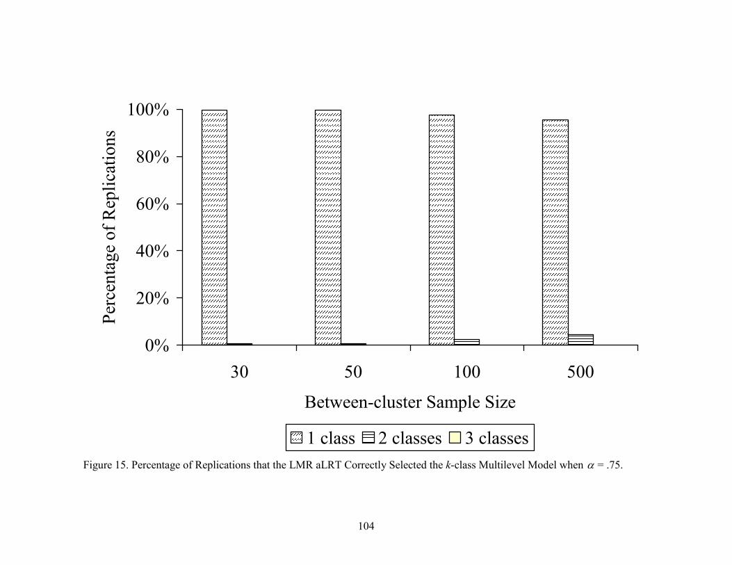
104

0%

20%

40%

60%

80%

100%

30 50 100 500

Between-cluster Sample Size

Perc

enta

ge o

f Rep

licat

ions

1 class 2 classes 3 classesFigure 15. Percentage of Replications that the LMR aLRT Correctly Selected the k-class Multilevel Model when α = .75.

105

0%

20%

40%

60%

80%

100%

30 50 100 500

Between-cluster Sample Size

Perc

enta

ge o

f Rep

licat

ions

1 class 2 classes 3 classesFigure 16. Percentage of Replications that the LMR aLRT Correctly Selected the k-class Multilevel Model when α = 1.0.

106

0%

20%

40%

60%

80%

100%

30 50 100 500

Between-cluster Sample Size

Perc

enta

ge o

f Rep

licat

ions

1 class 2 classes 3 classesFigure 17. Percentage of Replications that the LMR aLRT Correctly Selected the k-class Multilevel Model when α = 1.25.

107

0%

20%

40%

60%

80%

100%

30 50 100 500

Between-cluster Sample Size

Perc

enta

ge o

f Rep

licat

ions

1 class 2 classes 3 classesFigure 18. Percentage of Replications that the LMR aLRT Correctly Selected the k-class Single Level Model when α = .75.

108

0%

20%

40%

60%

80%

100%

30 50 100 500

Between-cluster Sample Size

Perc

enta

ge o

f Rep

licat

ions

1 class 2 classes 3 classesFigure 19. Percentage of Replications that the LMR aLRT Correctly Selected the k-class Single Level Model when α = 1.0.

109

0%

20%

40%

60%

80%

100%

30 50 100 500

Between-cluster Sample Size

Perc

enta

ge o

f Rep

licat

ions

1 class 2 classes 3 classesFigure 20. Percentage of Replications that the LMR aLRT Correctly Selected the k-class Single Level Model when α = 1.25.

110

Comparison of Fit Indices

The accuracy of the IC indices ranged from 83% to 100% when the factor mean

difference was equal to zero. Under the correctly specified MLCFA model, accuracy of

the BIC and aBIC remained relatively consistent, near 100%. Both the BIC and aBIC

outperformed the AIC across nearly all between-cluster sample size and ICC conditions

when the factor mean difference was equal to zero. The AIC behaved similarly to the

other ICs in that accuracy remained somewhat consistent across all conditions. When the

AIC did not lead to selection of the correct MLCFA model, the AIC typically led to

selection of the two-class MLFMM and occasionally the three-class MLFMM whereas

BIC incorrectly led to the selection of the SLCFA model. The LMR aLRT was more

accurate at selecting the correct one-class model for the correctly specified multilevel

models as compared the mis-specified single level models. The LMR aLRT had a greater

tendency to overestimate the number of classes for the mis-specified single level model

as compared to the multilevel models.

The accuracy of the IC indices decreased drastically when a factor mean

difference was introduced. Accuracy of the IC indices and the LMR aLRT, did however,

increase as the class separation and between-cluster sample size increased. The AIC

outperformed the BIC and aBIC under a correctly specified two-class MLFMM. The

aBIC had better accuracy than the BIC in leading to selection of the correct model and

discrepancy in performance of the two ICs was most pronounced in the larger class

separation conditions. The MLCFA was the most frequently selected model in all

conditions for all ICs when the correct model was not identified. The inaccurate

111

nonsignificant LMR aLRT for most conditions supports the high inaccuracy of the ICs.

The ICs and the LMR aLRT suggest that a one-class model is the plausible model, thus

underestimating the number of true classes, except when the class separation and

between-cluster sample size are greatest.

112

Table 4

Percentage of Occurrences (Out of the Converged Solutions) the Correct Model was Selected whenα = 0 and ICC = .10

Between-cluster Sample Size30 50 100 500

AIC BIC aBIC AIC BIC aBIC AIC BIC aBIC AIC BIC aBIC

Model 1 0 14 0 0 3 1 0 0 0 0 0 0Model 2 0 0 0 0 0 0 0 0 0 0 0 0Model 3 0 0 0 0 0 0 0 0 0 0 0 0Model 4* 87 86 97 86 97 97 88 99 98 90 100 100Model 5 8 0 3 12 0 2 12 1 2 10 0 0Model 6 5 0 0 2 0 0 0 0 0 0 0 0

Note. Model 1 = Single Level CFA Model. Model 2 = Single Level 2-Class Factor Mixture Model. Model 3 = Single Level 3-Class Factor Mixture Model. Model 4* = Correct Multi-level CFA Model. Model 5 = Multi-level 2-Class Factor MixtureModel. Model 6 = Multi-level 3-Class Factor Mixture Model.

113

Table 5

Percentage of Occurrences (Out of the Converged Solutions the Correct Model was Selected when α = 0 and ICC = .20

Between-cluster Sample Size30 50 100 500

AIC BIC aBIC AIC BIC aBIC AIC BIC aBIC AIC BIC aBIC

Model 1 0 1 0 0 0 0 0 0 0 0 0 0Model 2 0 0 0 0 0 0 0 0 0 0 0 0Model 3 0 0 0 0 0 0 0 0 0 0 0 0Model 4* 87 99 96 83 100 98 88 100 100 84 100 100Model 5 13 0 4 15 0 2 11 0 0 15 0 0Model 6 0 0 0 2 0 0 1 0 0 1 0 0

Note. Model 1 = Single Level CFA Model. Model 2 = Single Level 2-Class Factor Mixture Model. Model 3 = Single Level 3-Class Factor Mixture Model. Model 4* = Correct Multi-level CFA Model. Model 5 = Multi-level 2-Class Factor MixtureModel. Model 6 = Multi-level 3-Class Factor Mixture Model.

114

Table 6

Percentage of Occurrences (Out of the Converged Solutions) the Correct Model was Selected when α = .75 and ICC = .10

Between-cluster Sample Size30 50 100 500

AIC BIC aBIC AIC BIC aBIC AIC BIC aBIC AIC BIC aBIC

Model 1 0 6 0 0 1 0 0 0 0 0 0 0Model 2 0 0 0 0 0 0 0 0 0 0 0 0Model 3 0 0 0 0 0 0 0 0 0 0 0 0Model 4 79 93 95 82 99 99 80 100 96 85 100 100Model 5* 14 1 5 17 0 1 20 0 4 15 0 0Model 6 7 0 0 1 0 0 0 0 0 0 0 0

Note. * = N/A. Model 1 = Single Level CFA Model. Model 2 = Single Level 2-Class Factor Mixture Model. Model 3 = SingleLevel 3-Class Factor Mixture Model. Model 4 = Correct Multi-level CFA Model. Model 5* = Correct Multi-level 2-ClassFactor Mixture Model. Model 6 = Multi-level 3-Class Factor Mixture Model.

115

Table 7

Percentage of Occurrences (Out of the Converged Solutions) the Correct Model was Selected when α = .75 and ICC = .20

Between-cluster Sample Size30 50 100 500

AIC BIC aBIC AIC BIC aBIC AIC BIC aBIC AIC BIC aBIC

Model 1 0 0 0 0 0 0 0 0 0 0 0 0Model 2 0 0 0 0 0 0 0 0 0 0 0 0Model 3 0 0 0 0 0 0 0 0 0 0 0 0Model 4 79 100 96 76 100 99 93 99 97 82 100 98Model 5* 19 0 4 21 0 1 6 1 3 18 0 2Model 6 2 0 0 3 0 0 1 0 0 0 0 0

Note. Model 1 = Single Level CFA Model. Model 2 = Single Level 2-Class Factor Mixture Model. Model 3 = Single Level 3-Class Factor Mixture Model. Model 4 = Correct Multi-level CFA Model. Model 5* = Correct Multi-level 2-Class FactorMixture Model. Model 6 = Multi-level 3-Class Factor Mixture Model.

116

Table 8

Percentage of Occurrences (Out of the Converged Solutions) the Correct Model was Selected when α = 1.0 and ICC = .10

Between-cluster Sample Size30 50 100 500

AIC BIC aBIC AIC BIC aBIC AIC BIC aBIC AIC BIC aBIC

Model 1 1 15 3 0 1 0 0 0 0 0 0 0Model 2 0 0 0 0 0 0 0 0 0 0 0 0Model 3 0 0 0 0 0 0 0 0 0 0 0 0Model 4 76 85 89 79 99 97 66 100 98 33 98 92Model 5* 19 0 7 18 0 3 29 0 2 67 2 8Model 6 4 0 1 3 0 0 5 0 0 0 0 0

Note. Model 1 = Single Level CFA Model. Model 2 = Single Level 2-Class Factor Mixture Model. Model 3 = Single Level 3-Class Factor Mixture Model. Model 4 = Correct Multi-level CFA Model. Model 5* = Correct Multi-level 2-Class FactorMixture Model. Model 6 = Multi-level 3-Class Factor Mixture Model.

117

Table 9

Percentage of Occurrences (Out of the Converged Solutions) the Correct Model was Selected when α = 1.0 and ICC = .20

Between-cluster Sample Size30 50 100 500

AIC BIC aBIC AIC BIC aBIC AIC BIC aBIC AIC BIC aBIC

Model 1 0 0 0 0 0 0 0 0 0 0 0 0Model 2 0 0 0 0 0 0 0 0 0 0 0 0Model 3 0 0 0 0 0 0 0 0 0 0 0 0Model 4 75 100 94 84 98 96 65 99 92 35 99 91Model 5* 23 0 6 13 2 4 34 1 8 65 1 9Model 6 2 0 0 3 0 0 1 0 0 0 0 0

Note. * = N/A. Model 1 = Single Level CFA Model. Model 2 = Single Level 2-Class Factor Mixture Model. Model 3 = SingleLevel 3-Class Factor Mixture Model. Model 4 = Correct Multi-level CFA Model. Model 5* = Correct Multi-level 2-ClassFactor Mixture Model. Model 6 = Multi-level 3-Class Factor Mixture Model.

118

Table 10

Percentage of Occurrences (Out of the Converged Solutions) the Correct Model was Selected when α = 1.25 and ICC = .10

Between-cluster Sample Size30 50 100 500

AIC BIC aBIC AIC BIC aBIC AIC BIC aBIC AIC BIC aBIC

Model 1 1 18 5 0 2 1 0 0 0 0 0 0Model 2 0 0 0 0 0 0 0 0 0 0 0 0Model 3 0 0 0 0 0 0 0 0 0 0 0 0Model 4 63 82 83 49 93 81 22 86 59 0 2 0Model 5* 33 0 12 48 5 17 78 14 41 100 98 100Model 6 3 0 0 3 0 1 0 0 0 0 0 0

Note. * = N/A. Model 1 = Single Level CFA Model. Model 2 = Single Level 2-Class Factor Mixture Model. Model 3 = SingleLevel 3-Class Factor Mixture Model. Model 4 = Correct Multi-level CFA Model. Model 5* = Correct Multi-level 2-ClassFactor Mixture Model. Model 6 = Multi-level 3-Class Factor Mixture Model.

119

Table 11

Percentage of Occurrences (Out of the Converged Solutions) the Correct Model was Selected when α = 1.25 and ICC = .20

Between-cluster Sample Size30 50 100 500

AIC BIC aBIC AIC BIC aBIC AIC BIC aBIC AIC BIC aBIC

Model 1 0 2 0 0 0 0 0 0 0 0 0 0Model 2 0 0 0 0 0 0 0 0 0 0 0 0Model 3 0 0 0 0 0 0 0 0 0 0 0 0Model 4 50 91 79 37 97 77 16 91 64 0 9 1Model 5* 44 7 20 62 3 22 83 9 36 100 91 99Model 6 6 0 1 1 0 1 1 0 0 0 0 0

Note. * = N/A. Model 1 = Single Level CFA Model. Model 2 = Single Level 2-Class Factor Mixture Model. Model 3 = SingleLevel 3-Class Factor Mixture Model. Model 4 = Correct Multi-level CFA Model. Model 5* = Correct Multi-level 2-ClassFactor Mixture Model. Model 6 = Multi-level 3-Class Factor Mixture Model.

120

Table 12

Percentage of Occurrences the LMR aLRT Led to Selection of the Correct One-class Model for α = 0

Multilevel Single Level Number of Classes Number of Classes

1 2 3 1 2 3

ICC n*.10 30 99 0 1 96 3 1

50 100 0 0 94 4 2100 98 2 0 84 15 1500 94 4 2 88 8 4

.20 30 100 0 0 88 11 150 99 1 0 89 11 0

100 99 1 0 89 10 1500 95 5 0 93 6 1

Note. n* = Between-cluster Sample Size

121

Table 13

Percentage of Occurrences the LMR aLRT Led to Selection of the Correct Two-class Model for α = .75

Multilevel Single Level Number of Classes Number of Classes

1 2 3 1 2 3

ICC n*.10 30 99 1 0 92 5 3

50 100 0 0 99 1 0100 98 2 0 91 9 0500 96 4 0 92 5 3

.20 30 100 0 0 95 4 150 99 1 0 88 8 4

100 97 3 0 83 15 2500 95 5 0 84 16 0

Note. n* = Between-cluster Sample Size

122

Table 14

Percentage of Occurrences the LMR aLRT Led to Selection of the Correct Two-class Model for α = 1.0

Multilevel Single Level Number of Classes Number of Classes

1 2 3 1 2 3

ICC n*.10 30 99 0 1 98 2 0

50 100 0 0 91 6 3100 95 2 3 92 5 3500 68 32 0 96 4 0

.20 30 100 0 0 91 6 350 99 1 0 92 5 3

100 96 4 0 80 16 4500 65 35 0 78 17 5

Note. n* = Between-cluster Sample Size

123

Table 15

Percentage of Occurrences the LMR aLRT Led to Selection of the Correct Two-class Model for α = 1.25

Multilevel Single Level Number of Classes Number of Classes

1 2 3 1 2 3

ICC n*.10 30 100 0 0 92 4 4

50 95 5 0 85 14 1100 70 28 2 65 31 4500 0 100 0 92 4 4

.20 30 97 3 0 82 16 250 96 4 0 92 8 0

100 66 34 0 87 12 1500 0 100 0 25 66 9

Note. n* = Between-cluster Sample Size

124

Parameter and Standard Error Estimate Bias

Parameter Estimate Bias

The relative bias of factor loading estimates within-cluster ( Wλ ) and between-

cluster ( Bλ ), factor variance estimates within-clusters ( Wψ ) and between-clusters ( Bψ ),

error variance estimates within-cluster [ )( WVar ε ], and the factor mean estimate (α ) were

computed for the correct model and are presented in Tables 16 to 19. Substantial

parameter estimate bias was identified for any parameter estimate when

05.|)ˆ(| >θB (Hoogland & Boomsma, 1998).

Across all MLCFA and MLFMM conditions, the within-cluster factor loading

estimates and error variance estimates demonstrated acceptable bias. Factor loading

estimation bias ranged from -1.4% to 3.7% and error variance estimation bias ranged

from -2.6% to .8%. The absolute bias of the average factor loading estimates was .7%

and .5% for the average error variance estimates across all within-factor loading

estimates and error variance estimates Bias of the within-cluster factor variance

estimates under MLCFA generating conditions also demonstrated acceptable bias ranging

from -.8% to .9%. Conversely, for MLFMM generating conditions, the within-cluster

factor variance estimates demonstrated consistently negative bias, but bias decreased as

class separation and between-cluster sample size increased. Bias ranged from -24% to

2%. ICC had little impact on bias of the within-cluster factor variance estimate. On

average, across ICC values and factor mean differences, absolute bias ranged from 1%

(between-cluster sample size = 500) to 15% (between-cluster sample size = 30). The

125

negative bias in the within-cluster factor variance estimate suggests that the estimate was

consistently underestimated during model estimation.

Similar to within-cluster factor loading estimates, across all MLCFA and

MLFMM conditions, there was no evidence of between-cluster factor loading estimation

bias. Factor loading estimation bias ranged from -2.5% to 1.5%. The absolute bias of the

average factor loading estimates was .4% across all between-cluster factor loading

estimates. Bias of the between-cluster factor variance estimates under MLCFA

generating conditions also demonstrated acceptable bias ranging from -3.7% to 2.2%.

Conversely, for MLFMM generating conditions, the between-cluster factor variance

estimates demonstrated consistently negative bias under various conditions, ranging from

-15% to 3%. As class separation increased, bias was more pronounced across conditions

when ICC = .10. On average, however, across ICC values and factor mean differences,

absolute bias ranged from 3% (between-cluster sample size = 500) to 7% (between-

cluster sample size = 30). The negative bias in the between-cluster factor variance

suggests that the estimate was consistently underestimated during model estimation. The

factor mean estimation bias was largely unacceptable and inconsistent across the

conditions. Across ICC and factor mean difference conditions, the absolute bias tended to

decrease as between-cluster sample size increased, ranging from 15% (between-cluster

sample size = 100) to 36% (between-cluster sample size = 30). However, the average

absolute bias for the largest between-cluster sample size condition did not follow that

decreasing pattern and increased to 38%.

126

Table 16

Relative Bias of Estimated Parameters for the Correct Model with 0=α for ICC = .10 and ICC = .20

ICC = .10 ICC = .20 Between-cluster Sample Size Between-cluster Sample Size 30 50 100 500 30 50 100 500

Parameter

2Wλ .002 .005 .004 -.001 .004 .004 .002 .002

3Wλ -.001 .001 .003 -.002 -.004 .013 -.002 .000

4Wλ .001 .003 -.003 .000 -.006 .006 -.002 .001

2Bλ .003 -.009 -.013 .001 .005 -.001 .007 .0003Bλ .009 .008 -.004 -.003 .000 .003 .003 .001

4Bλ -.009 .005 -.003 .003 .004 -.002 .004 -.001VAR( 1Wε ) -.003 -.001 -.003 -.002 -.004 .006 -.004 .002VAR( 2Wε ) -.009 -.005 -.002 -.001 -.006 -.009 -.001 -.001VAR( 3Wε ) -.014 -.004 -.001 .001 -.006 .000 -.004 .000VAR( 4Wε ) -.004 -.009 .000 .000 -.011 -.004 .002 .001

Wψ -.008 -.005 -.002 .004 .009 -.001 .001 -.002

Bψ -.036 -.036 -.005 -.006 -.037 .022 -.012 .000

Note. Wλ = Within-cluster Factor Loading Estimate; Bλ = Between-cluster Factor Loading Estimate; VAR( Wε ) = Within-cluster Residual Variance Estimate; Wψ = Within-cluster Factor Variance Estimate; Bψ = Between-cluster Factor Variance Estimate.

127

Table 17 Relative Bias of Estimated Parameters for the Correct Model with 75.=α for ICC = .10 and ICC = .20

ICC = .10 ICC = .20 Between-cluster Sample Size Between-cluster Sample Size 30 50 100 500 30 50 100 500

Parameter

2Wλ .026 .002 .010 .002 .008 -.009 -.002 -.003

3Wλ .001 -.005 .003 .004 .003 -.009 .001 -.003

4Wλ .012 .010 -.002 .004 .015 -.006 .003 -.002

2Bλ -.025 .002 -.002 -.002 .006 .008 -.001 .0023Bλ -.002 -.006 -.004 -.003 .012 .009 -.005 .003

4Bλ -.010 -.004 .007 -.004 .010 .005 .000 .001α .672 -.114 .194 .300 .647 .595 .159 .351

VAR( 1Wε ) -.021 -.002 -.009 .001 -.005 -.011 -.004 .001VAR( 2Wε ) -.026 -.006 -.008 .000 .005 -.005 .004 .000VAR( 3Wε ) -.001 -.001 -.001 .002 -.006 .001 .007 -.001VAR( 4Wε ) -.017 -.001 -.002 -.002 -.004 -.005 -.002 -.001

Wψ -.203 -.141 -.085 -.016 -.238 -.149 -.098 -.018

Bψ .032 -.034 -.004 -.010 -.060 -.023 .002 -.021

Note. Wλ = Within-cluster Factor Loading Estimate; Bλ = Between-cluster Factor Loading Estimate; α = Factor Mean Difference; VAR( Wε ) = Within-cluster Residual Variance Estimate; Wψ = Within-cluster Factor Variance Estimate; Bψ = Between-cluster Factor Variance Estimate.

128

Table 18

Relative Bias of Estimated Parameters for the Correct Model with 0.1=α for ICC = .10 and ICC = .20

ICC = .10 ICC = .20 Between-cluster Sample Size Between-cluster Sample Size 30 50 100 500 30 50 100 500

Parameter

2Wλ .024 .005 .010 .000 .010 .009 .003 .002

3Wλ .015 .016 .003 -.002 .028 .011 -.005 .003

4Wλ .013 .004 .002 -.001 .018 .002 -.001 .003

2Bλ -.006 -.001 .004 .003 .004 .006 .001 .0033Bλ .002 -.002 -.004 .004 -.001 -.004 .003 .001

4Bλ .004 .006 .005 .002 -.006 .004 .002 .003α .336 .016 -.099 -.064 .328 -.117 -.133 -.474

VAR( 1Wε ) -.007 -.009 .002 .001 -.005 -.006 -.003 .001VAR( 2Wε ) -.011 -.006 -.007 .001 -.013 -.014 -.005 -.002VAR( 3Wε ) -.010 -.007 -.003 .001 -.015 -.012 -.001 -.001VAR( 4Wε ) -.006 .001 -.002 -.002 -.002 -.001 -.001 .000

Wψ -.118 -.073 -.023 .010 -.125 -.061 -.045 -.008

Bψ -.104 -.052 -.054 -.043 -.023 -.021 -.027 -.015

Note. Wλ = Within-cluster Factor Loading Estimate; Bλ = Between-cluster Factor Loading Estimate; α = Factor Mean Difference; VAR( Wε ) = Within-cluster Residual Variance Estimate; Wψ = Within-cluster Factor Variance Estimate; Bψ = Between-cluster Factor Variance Estimate.

129

Table 19

Relative Bias of Estimated Parameters for the Correct Model with 25.1=α for ICC = .10 and ICC = .20

ICC = .10 ICC = .20 Between-cluster Sample Size Between-cluster Sample Size 30 50 100 500 30 50 100 500

Parameter

2Wλ .024 .005 -.003 -.003 .022 -.007 .004 -.002

3Wλ .008 -.014 -.011 .000 .026 -.011 .009 -.003

4Wλ .013 .012 -.005 -.005 .037 -.008 .011 .003

2Bλ .009 -.011 -.001 .001 .007 .000 .002 .0013Bλ .015 .011 .000 -.001 .001 -.003 .002 .001

4Bλ .012 .009 .005 .002 .004 .002 .005 .000α .131 -.741 .012 .036 .019 .041 -.294 -1.077

VAR( 1Wε ) -.016 -.004 -.003 -.001 -.007 -.010 -.002 .000VAR( 2Wε ) -.015 -.012 .004 -.001 .005 -.001 .002 .003VAR( 3Wε ) -.014 .008 .000 -.001 -.005 -.002 -.003 .000VAR( 4Wε ) -.017 -.014 -.003 .003 .000 -.007 -.008 .001

Wψ .019 .006 -.004 -.020 -.090 -.013 -.020 -.016

Bψ -.151 -.054 -.054 -.059 -.070 -.025 -.041 -.037

Note. Wλ = Within-cluster Factor Loading Estimate; Bλ = Between-cluster Factor Loading Estimate; α = Factor Mean Difference; VAR( Wε ) = Within-cluster Residual Variance Estimate; Wψ = Within-cluster Factor Variance Estimate; Bψ = Between-cluster Factor Variance Estimate.

130

Standard Error Estimate Bias

The relative bias of the standard error estimates for the factor loadings within-

cluster ( Wλ ) and between-cluster ( Bλ ), factor mean )(α , factor variances within-cluster

( Wϕ ) and between-cluster ( Bϕ ), and error variances within-cluster [ )( WVar ε ] were

computed for the correct model and are presented in Tables 20 to 23. Substantial standard

error estimate bias was identified for any standard error as 1.0|)ˆ(| ˆ >θ

esB (Hoogland &

Boomsma, 1998).

Both positive and negative bias of the standard error estimates was present in the

within-cluster factor loadings. Under MLCFA generating conditions, standard error

estimate bias was largely unacceptable for within-cluster factor loadings ranging from -

13% to 18% when ICC = .10. When ICC = .20, the standard error estimates demonstrated

minimal bias ranging from -9% to 6%. The average absolute bias for ICC = .10 and ICC

= .20 was, however acceptable at 9% and 6%, respectively. Under MLFMM generating

conditions, the ICC and factor mean difference conditions appeared to have little impact

on bias of the within-cluster factor loading standard error estimates. Relative bias ranged

from -15% to 65% and tended to decrease as between-cluster sample sizes increased. The

average absolute bias was, however, unacceptable only when the between-cluster sample

size was the smallest, ranging from 5% in the largest between-cluster sample size

condition to 18% in the smallest between-cluster sample size condition.

The within-cluster standard error estimates for the error variances also

demonstrated positive and negative bias and varied across the conditions. Under MLCFA

generating conditions, bias ranged from -12% to 16% where bias had a tendency to be

131

negative and increase slightly as between-cluster size increased. The absolute bias ranged

from 5% in the smallest between-cluster size condition to 7% in the largest between-

cluster sample size condition. On average, the absolute bias was acceptable for all

between-cluster sample sizes. Under MLFMM generating conditions, relative bias of the

within-cluster error variance standard error estimates ranged from -15% to 40%. ICC

values and factor mean difference conditions appeared to have little influence on bias, but

bias had a tendency to decrease as between-cluster sample size increased. On average, the

absolute bias across all between-cluster sample size conditions was acceptable ranging

from 6% (between-cluster sample size = 500) to 8% (between-cluster sample size = 30).

Under MLCFA generating conditions, the within-cluster factor variance standard

error estimate demonstrated positive and negative bias ranging from -17% to 8% with no

consistent pattern across the conditions. On average, across all within-cluster factor

variance standard error estimates, the absolute bias, however, was acceptable at 9%.

Under MLFMM generating conditions, in general, bias of the within-cluster factor

variance standard error estimate was positive and ranged from -24% to 301%. Bias

tended to decrease with an increase in class separation, ICC values, and between-cluster

sample size conditions. On average, the absolute bias ranged from a low of 14% when the

between-cluster sample size was greatest to a high of 75% when the between-cluster

sample size was smallest.

Similar to the within-cluster factor loading standard error estimate bias, under

MLCFA generating conditions, the between-cluster factor loading standard error

estimates demonstrated positive and negative bias ranging from -16% to 10% where bias

132

had a tendency to decrease when between-cluster sample size increased. On average, the

absolute bias ranged from a 3% to 10% for the largest to smallest between-cluster sample

size conditions, respectively. Under MLFMM generating conditions, positive and

negative bias was present in the between-cluster factor loading standard error estimates,

ranging from -21% to 116%. As between-cluster sample size increased, bias generally

decreased. On average, the absolute bias ranged from 7% when the between-cluster size

was the largest to 17% when the between-cluster size was the smallest.

The between-cluster factor variance standard error estimates demonstrated

minimal negative bias for most conditions under MLCFA generating conditions, ranging

from -12% to -1%. The consistent negative bias, although negligible, indicates that the

between-cluster factor variance standard error estimates are typically underestimated

during estimation. Bias under MLFMM generating conditions, tended to be negative and

in most conditions minimal ranging from -11% to 37%. On average, the absolute bias

ranged from 4% to 14% where the greatest amount of bias was present in the smallest

between-cluster sample size condition.

No clear pattern was evident in the bias of the factor mean standard error

estimates, ranging from -96% to over 3000%. On average, absolute bias ranged from

540% in the smallest between-cluster sample size condition to 60% in the largest

between-cluster sample size condition. The instability of the standard error estimates

suggests the need for more replications.

Few clear patterns were evident in the bias of the standard error estimates. In

general, relative bias of the within- and between-cluster parameter standard error

133

estimates was demonstrated across many of the conditions, but tended to decrease as

between-cluster sample size increased. Average absolute bias, was largely acceptable

across most conditions.

134

Table 20

Relative Bias of Standard Error Estimates for the Correct Model with 0=α for ICC = .10 and ICC = .20

ICC = .10 ICC = .20 Between-cluster Sample Size Between-cluster Sample Size 30 50 100 500 30 50 100 500

Parameter

2Wλ -.105 -.044 .152 -.080 -.079 .064 .021 -.063

3Wλ -.088 .180 .030 .066 .059 -.082 -.056 -.046

4Wλ -.130 -.016 .067 .094 .035 -.094 -.080 .051

2Bλ -.059 -.113 -.097 .069 -.054 -.004 .031 .0193Bλ -.119 -.159 -.023 .032 -.127 .015 .100 -.020

4Bλ -.146 -.063 -.010 -.002 -.101 -.061 -.050 -.042VAR( 1Wε ) -.049 -.090 .084 .164 -.043 -.036 -.114 -.079VAR( 2Wε ) -.099 -.086 .048 -.124 -.067 .120 -.025 -.078VAR( 3Wε ) -.051 -.050 -.012 -.021 -.013 .035 -.041 .025VAR( 4Wε ) -.061 .099 -.065 .047 -.043 -.008 -.080 -.020

Wψ -.170 .047 .121 -.111 -.108 -.002 .078 .083

Bψ -.032 -.103 -.071 -.077 -.012 -.031 -.115 -.044

Note. Wλ = Within-cluster Factor Loading Estimate; Bλ = Between-cluster Factor Loading Estimate; VAR( Wε ) = Within-cluster Residual Variance Estimate; Wψ = Within-cluster Factor Variance Estimate; Bψ = Between-cluster Factor Variance Estimate.

135

Table 21

Relative Bias of Standard Error Estimates for the Correct Model with 75.=α for ICC = .10 and ICC = .20

ICC = .10 ICC = .20 Between-cluster Sample Size Between-cluster Sample Size 30 50 100 500 30 50 100 500

Parameter

2Wλ .197 .291 -.082 .016 .338 -.051 -.012 -.067

3Wλ .211 .049 -.074 .021 .361 -.059 .061 .005

4Wλ .038 .247 .000 .043 .001 -.037 .126 -.005

2Bλ .010 .229 -.097 .015 -.015 -.056 -.070 -.1183Bλ .012 .113 .106 .118 .016 -.030 -.105 .048

4Bλ -.075 .052 -.044 -.053 -.023 .022 -.035 .081α .344 -.587 -.670 -.581 .940 .672 -.465 .284

VAR( 1Wε ) -.022 .258 .045 .035 .083 .037 .029 -.036VAR( 2Wε ) .146 -.009 -.009 -.029 -.011 .069 -.074 -.015VAR( 3Wε ) .141 -.078 -.031 -.003 -.012 -.022 .050 .026VAR( 4Wε ) .126 .021 -.075 .154 .129 .029 -.062 .045

Wψ .403 .304 -.243 .041 .565 .310 .637 .622

Bψ .165 -.013 -.114 -.010 -.038 -.093 .060 .039

Note. Wλ = Within-cluster Factor Loading Estimate; Bλ = Between-cluster Factor Loading Estimate; α = Factor Mean Difference; VAR( Wε ) = Within-cluster Residual Variance Estimate; Wψ = Within-cluster Factor Variance Estimate; Bψ = Between-cluster Factor Variance Estimate.

136

Table 22

Relative Bias of Standard Error Estimates for the Correct Model with 0.1=α for ICC = .10 and ICC = .20

ICC = .10 ICC = .20 Between-cluster Sample Size Between-cluster Sample Size 30 50 100 500 30 50 100 500

Parameter

2Wλ .533 .110 -.014 -.144 -.041 .128 .141 .056

3Wλ .209 -.030 .080 .031 -.135 .061 .075 .011

4Wλ .647 -.020 .059 .009 -.061 .066 .123 .018

2Bλ .639 -.027 -.040 -.080 -.213 .021 .055 .0143Bλ 1.165 .148 -.023 -.076 -.172 -.068 .053 -.029

4Bλ .291 .028 -.015 -.072 -.106 -.156 .157 .025α 30.338 -.628 -.550 -.762 -.019 -.588 -.647 -.862

VAR( 1Wε ) -.039 .041 -.065 .049 -.086 .042 -.069 .017VAR( 2Wε ) .404 .080 -.085 .006 -.023 .001 .034 .000VAR( 3Wε ) .017 .101 .085 .101 -.045 .039 .017 -.061VAR( 4Wε ) .204 .207 -.010 .076 .055 -.044 -.122 -.022

Wψ 3.099 .227 .477 -.050 .092 .171 .075 .069

Bψ .370 .066 -.045 -.077 -.080 -.036 .045 .056

Note. Wλ = Within-cluster Factor Loading Estimate; Bλ = Between-cluster Factor Loading Estimate; α = Factor Mean Difference; VAR( Wε ) = Within-cluster Residual Variance Estimate; Wψ = Within-cluster Factor Variance Estimate; Bψ = Between-cluster Factor Variance Estimate.

137

Table 23

Relative Bias of Standard Error Estimates for the Correct Model with 25.1=α for ICC = .10 and ICC = .20

ICC = .10 ICC = .20 Between-cluster Sample Size Between-cluster Sample Size 30 50 100 500 30 50 100 500

Parameter

2Wλ -.008 .036 .048 .120 -.069 .085 -.015 .044

3Wλ -.014 .034 .137 .067 .056 .031 .016 -.147

4Wλ .100 -.001 -.015 .141 -.122 -.039 -.058 -.007

2Bλ -.137 .028 .115 .040 -.041 -.013 -.010 .0533Bλ -.065 -.010 .055 .110 .028 .057 -.024 -.096

4Bλ -.012 -.164 .146 .185 -.069 .039 -.027 -.024α -.326 -.797 -.493 .083 -.636 -.705 -.871 -.960

VAR( 1Wε ) -.090 .003 -.136 -.007 .057 .091 .122 -.045VAR( 2Wε ) -.075 .052 -.137 .182 .003 -.002 -.154 -.102VAR( 3Wε ) .066 -.022 .111 -.103 -.152 .039 .087 .234VAR( 4Wε ) .098 .008 -.114 .018 -.042 .089 .170 .107

Wψ .256 .416 .149 .039 -.092 .039 .025 -.041

Bψ -.045 -.019 -.002 .108 -.110 -.024 -.108 -.008

Note. Wλ = Within-cluster Factor Loading Estimate; Bλ = Between-cluster Factor Loading Estimate; α = Factor Mean Difference; VAR( Wε ) = Within-cluster Residual Variance Estimate; Wψ = Within-cluster Factor Variance Estimate; Bψ = Between-cluster Factor Variance Estimate.

138

Chapter V: Discussion

The current study was designed to assess the performance of common fit indices

used to test the plausibility of CFA models that both model the nonindependence of data

gathered from clustered sampling designs and model unobserved heterogeneity through

latent classes. Additionally, parameter and standard error estimate bias of correctly

specified MLCFA and MLFMM models was investigated. Discussion of the results will

be presented in order of the previous chapter including a summary of the issues

surrounding the convergence rates, performance of the AIC, BIC, aBIC, and LMR aLRT

followed by bias of the parameters and standard error estimates. The chapter will

conclude with a discussion of the implications of the findings, recommendations for

applied research, and finally, limitations to the current study, recommendations for future

research, and a general conclusion.

Convergence Problems

Convergence problems were frequently encountered especially when class

separation and between-cluster sample sizes were small for the conditions studies in the

current study. Although all correctly specified MLCFA converged in the current study,

nonconvergence of the MLFMM as a result of small between-cluster sample sizes was

consistent with those found in other MLCFA simulation studies (Hox & Maas, 2001;

Muthén & Satorra, 1995). Little, if any, research has been reported regarding factors

influencing convergence rates in MLFMM. One of the most important factors influencing

convergence of MLFMM appears to be the magnitude of the difference in factor means

among the latent classes, where larger differences result in greater convergence.

139

Similarly, larger between-cluster sample sizes (i.e., between-cluster sample size = 100,

500) appear to positively influence convergence rates. An additional factor affecting

nonconvergence was the incorrect specification of models. The high nonconvergence

rates of the mis-specified three-class MLFMM may have significance in an applied

research setting. Specifically, while the number of true latent classes is unknown in

applied research, an applied researcher can be somewhat confident that if model

estimation does not converge for a selected k-class model then it seems more likely that a

model with fewer classes may better represent the data.

Performance of the Fit Indices

Performance of the more commonly used IC indices (AIC, BIC, aBIC) were

evaluated to identify which of the indices more often led to the selection of the correct

model. An additional index of fit appropriate for comparing models that are not nested

such as models with differing number of latent classes is the LMR aLRT. The LMR

aLRT is a statistical test used to assess whether the k-class model is supported over the

corresponding (k-1)-class model. Performance of all fit indices was evaluated as a

function of varying ICC levels, factor mean differences, and between-cluster sample

sizes.

In general, when latent classes are not hypothesized and thus data are generated to

fit a MLCFA model, the BIC and aBIC are more accurate fit indices than the AIC.

Accuracy of the fit indices is consistent for both small and large ICC values and a range

of between-cluster sample sizes. Moreover, if latent classes are hypothesized, across

nearly all MLCFA generating conditions, the LMR aLRT tends to support the IC indices

140

suggesting that a one-class model sufficiently describes the data. The LMR aLRT had a

slight tendency to overestimate the correct number of latent classes when the incorrect

SLCFA models were specified.

Conversely, for data generated to fit a correct two-class MLFMM, accuracy of the

IC indices and the LMR aLRT declined. Although the AIC minimally outperformed the

BIC and aBIC, in general, the IC indices and the LMR aLRT typically lead to selection of

the mis-specified MLCFA, again, suggesting a one-class model. The accuracy of the fit

indices, did however, increase mainly as a function of an increase in class separation and

between-cluster sample size to near 100% in the largest factor mean difference and

between-cluster sample size condition. For a majority of the conditions studied in the

current study, the fit indices have a tendency to underestimate the number of latent

classes. The inability of the LMR aLRT to detect better fit of the correct two-class model

over a one-class model indicates presence of a high Type II error rate. In other words, the

nonsignificant LMR aLRT for the correct two-class MLFMM across a majority of the

conditions, results when one concludes that the one-class model fits better when the two-

class model better captures the heterogeneity of the data.

As literature on the performance of the AIC, BIC, aBIC and the LMR aLRT for

MLFMM is sparse, supporting or opposing evidence for the present findings is lacking.

Rather, attention can be drawn towards the findings from single level LCA models and

LCA models that correct for standard error estimate bias as a result of nested data (i.e.,

design-based analysis) as opposed to modeling the data hierarchy. Specifically, when

comparing among the AIC, BIC, and aBIC in both single-level and design-based LCA

141

models (Clark & Muthén, 2007; Nylund et al., 2006), the AIC performed poorly which

supports the current findings except for conditions of large class separation and between-

cluster sample sizes. Interestingly, although the performance of the AIC was typically

poor, the AIC outperformed both the BIC and aBIC in the current study, which does not

support the results of Nylund et al. (2006) or Clark and Muthén (2007). Moreover, the

aBIC slightly outperformed the BIC, which is also not consistent with the previously

mentioned research findings. Several factors could be partly responsible for the

differences in the results. Nylund et al. (2006) and Clark and Muthén (2007) studied LCA

models as opposed to the current study that included a continuous latent factor to explain

the relationships between the observed variables. Further, the current study only

investigated continuous observed items whereas Nylund et al. (2006) used continuous

and categorical items and Clark and Muthén (2007) used categorical items only.

Interestingly, results from the different analyses of the categorical items did not

necessarily result in similar findings.

The sample sizes and nature of the clustering were very different among the

current study and Clark and Muthén (2007). Clark and Muthén (2007) studied

performance of the ICs when nesting of the data were small numbers of observations

within larger contexts and accounted for the nonindependence of the data differently than

in the current study. The inconclusive results suggest that no one single fit index appears

to be optimal in selecting the correct model for single level or multilevel models that

include latent classes.

142

Parameter and Standard Error Estimate Bias

Bias in factor loading estimates within-and between-clusters, within-cluster error

variance estimates, and bias in within-cluster factor variance estimates for the correct

MLCFA model were acceptable across all MLCFA generating conditions. Negligible

bias of the within-and between-cluster parameter estimates supports the work of Muthén

and Satorra (1995) and Hox and Maas (2001) who also reported minimal bias of the

within- and between-cluster factor loading, error variance, and factor variance estimates

for a correctly specified MLCFA model.

Under MLFMM generating conditions, the bias of the within-cluster factor

variance estimate was consistently negative, but decreased with increasing class

separation and between-cluster sample size. When the absolute bias was averaged across

the factor mean difference and ICC values, bias was unacceptable only in the smallest

between-cluster sample size condition. Negative between-cluster factor variance

estimation bias was more prevalent under low ICC and moderate and high factor mean

difference conditions. The negative relationship between between-cluster sample size and

between-cluster factor variance estimation bias suggests that larger sample sizes between-

clusters results in lower estimation bias. When the absolute bias was averaged across the

factor mean difference and ICC values, the average absolute bias was, however,

acceptable for all between-cluster sample size conditions.

In contrast to the negligible bias of the parameters estimates, nonnegligible

standard error estimation bias was present for within-cluster factor loadings, error

variances, and factor variances when the correct generating model was a MLCFA. In

143

general, bias tended to decrease as between-cluster sample size increased. In general,

however, on average across ICC values and factor mean difference conditions, absolute

bias of standard error estimation of the within-cluster factor loadings was acceptable

which supports the minimal bias found in within-cluster parameter standard error

estimates by Hox and Maas (2001) and Muthén and Satorra (1995). Bias in within-cluster

parameter standard error estimates under MLFMM generating conditions demonstrated

bias across many conditions, but tended to decrease as between-cluster sample size

increased. The absolute bias average across ICC and factor mean difference conditions

generally was acceptable, especially when between-cluster sample size was large. Bias of

the between-cluster parameter standard error estimates was largely unacceptable across

all conditions, but tended to decrease with an increase in between-cluster sample size

which supports the findings of Hox and Maas (2001) and Muthén and Satorra (1995).

The trends of the standard error estimate bias appear to be in line with previous research

in that bias decreases with an increase in between-cluster sample sizes. It is again

emphasized, however, that estimation bias was only studied in correctly specified

MLCFA and MLFMM. The inconsistency in direction of bias of stability of estimates

suggests that more replications are needed to better understand the behavior of the

estimates.

Implications and Recommendations

Based on the results of the current study, the performance of the fit indices varied

primarily as a function of class separation and between-cluster sample size. That is, if the

plausibility of latent classes is explored when it is likely that one population best

144

describes the data, the BIC and aBIC are the best indicators of the most plausible model.

If data are nested and modeled appropriately, the LMR aLRT is also a good indicator that

a one-class model is sufficient to describe the data. The accuracy of the BIC, aBIC, and

LMR aLRT is consistent across a range of between-cluster sample sizes.

On the other hand, if the plausibility of latent classes is explored when it is likely

that more than one population best describes the data, more often than not, the fit indices

will underestimate the number of latent classes. When nested data are modeled

appropriately, the LMR aLRT and to some extent the AIC are better indicators of the

number of latent classes that best describe the data. However, the accuracy of both

indices is dependent upon a large discrepancy between the latent classes (i.e., factor mean

difference = 1.25) and large between-cluster sample sizes (i.e., between-cluster sample

size = 500). Researchers are urged to examine both IC indices and the LMR aLRT when

investigating latent classes.

Replicating the ideal conditions according to the results found in the current study

for which the fit indices are nearly 100% accurate may be challenging. Although one’s

confidence of a k-class model can increase with increasing class separation, class

separation can not be increased through manipulation in applied research. Although not

studied in the current study, two considerations are worth noting. First, researchers

should introduce a meaningful covariate as a means of increasing class separation. As

Lubke and Muthén (2007) reported, the proportion of correctly classified observations

increased with increasing covariate effects. As they demonstrated with the LMR aLRT,

perhaps performance of the IC indices would also increase with the addition of a

145

meaningful covariate. Second, rather than modeling invariant classes, examine models

where intercepts are free to vary across classes. Lubke and Muthén (2007) also reported

an increased proportion of correctly classified observations when class-specific intercepts

were modeled. In sum, if factor mean differences alone are relatively small, researchers

should investigate the use of covariates and non-invariant class models as a way to

increase class separation.

The high rates of nonconvergence for mis-specified three-class models also

indicate that it is unlikely that a k+1-class model best represents the data. When high rates

of nonconvergence are encountered, fewer latent classes should be specified. Conclusions

based upon model parsimony should not be disregarded when including latent classes.

Limitations and Suggestions for Future Research

Inherent in any research are factors by which the research is limited. Given that,

the current study only considers factor loadings of one magnitude, (albeit sufficient for

construct validity). Moreover, the factor loadings at the within- and between-cluster level

are the same, which may not necessarily reflect realistic applied conditions. Future

research should incorporate varying levels of within- and between-cluster factor loadings.

The simplicity of the 4-item factor at both the within- and between-cluster level

likely under-represents the complexity of many social science phenomena, thus

potentially limiting the generalizability of the performance of the fit indices. Model

complexity, in terms of the number of latent classes specified, could also be extended.

The current research was limited to the study of correctly specified one- and two-class

146

MLFMM. Future research should consider varying levels of model complexity and their

impact on accuracy of fit indices.

The between-cluster sample size conditions evaluated in the current study were

selected to reflect more typical conditions in applied research. Nonetheless, sample size

within-cluster was modeled as constant across all conditions which is likely an unrealistic

assumption. Although estimation procedures have been developed to account for unequal

within-cluster sample sizes (Muthén, 1994) and research has demonstrated that the

between-cluster sample size as opposed to within-cluster sample size is more influential

on convergence rates and parameter and standard error estimation bias (Hox & Maas,

2001), it is unknown how performance of the fit indices and bias may change when

unequal within-cluster sample sizes are introduced in MLFMM.

The appropriateness of factor mean comparison across groups hinges on the

degree of measurement invariance, although uncertainty regarding the optimal degree

still exists. The present study assumed strict measurement invariance and although

suitable to compare factor means across latent classes, strong invariance (i.e., invariant

factor loadings and intercepts) may be more realistic and still acceptable when comparing

factor means. Introducing intercept differences may assist in the ability of the ICs and/or

the LMR aLRT to correctly identify the correct number of latent classes. While Lubke

and Muthén (2007) did not measure accuracy of fit indices, they demonstrated that class-

specific intercepts led to increased accuracy in correctly classifying observations to latent

classes. Future research should consider partial measurement invariance to determine its

impact on performance of fit indices in MLFMM.

147

In addition to the fit indices evaluated in the current study, other IC indices have

been proposed to compare nonnested models, such as those with differing number of

latent classes. The fit indices (e.g., AIC, BIC, aBIC, LMR aLRT) selected for this study

are more commonly used and are readily available in software packages such as Mplus.

Other less commonly used fit indices such as the Consistent AIC (CAIC; Bozdogan,

1987) or the bootstrap likelihood ratio test (BLRT) demonstrate potential in identifying

the correct number of latent classes among single level latent class models (Nylund et al.,

2006) and should be investigated in MLFMM.

General Conclusion

The present research focused on the merging of two families of models that have

been around for decades and that are now more accessible with advancements in software

and computer technology. Specifically, the current study investigated models that

combined appropriately modeled nonindependence of data that can result from multistage

sampling designs along with the modeling of unobserved heterogeneity. While theory and

parsimony should not be disqualified, fit indices offer one way of investigating the

number of latent classes among plausible alternatives. The performance of the fit indices

evaluated here suggest that under a model-based design, the AIC and the LMR aLRT are

the most accurate among the set of indices investigated when class separation and

between-cluster sample size are large or for the current study, when factor mean

difference = 1.25 and between-cluster sample size = 500. It is hoped that the current

study introduces applied researchers to different modeling techniques that are most

appropriate for their interests and provides insight into optimal fit indices under various

148

realistic modeling conditions. Further, it is hoped that the current research has

encouraged continued investigation of identifying the best measures to assess the most

plausible number of latent classes in multilevel models.

149

References

Akaike, H. (1987). Factor analysis and AIC. Psychometrika, 52, 317-332.

Alwin, D. F., & Jackson, D. J. (1981). Applications of simultaneous factor analysis to

issues of factorial invariance. In D. J. Jackson & E. P. Borgotta (Eds.), Factor

analysis and measurement in sociological research: A multidimensional

perspective. Beverly Hills, CA: Sage.

Amemiya, T. (1985). Advanced econometrics. Cambridge, MA: Harvard University

Press.

Arminger, G., Stein, P., & Wittenberg, J. (1999). Mixtures of conditional mean and

covariance structure models. Psychometrika, 64, 475–494.

Asparouhov, T., & Muthén, B. O. (2006). Multilevel mixture models. Unpublished

manuscript.

Bandeen-Roche, K., Miglioretti, D. L., Zeger, S. L., & Rathouz, P. J. (1997). Latent

variable regression for multiple discrete outcomes. Journal of the American

Statistical Association, 92, 1375-1386.

Bauer, D. J., & Curran, P. J. (2003a). Distributional assumptions of growth mixture

models. Implications for overextraction of latent trajectory classes. Psychological

Methods, 8, 338-363.

Bauer, D. J., & Curran, P. J. (2003b). Overextraction of latent trajectory classes: Much

ado about nothing? Reply to Rindskopf (2003), Muthén (2003), and Cudeck and

Henly (2003). Psychological Methods, 8, 384-393.

Bauer, D. J., & Curran, P. J. (2004). The integration of continuous and discrete latent

150

variable models: Potential problems and promising opportunities. Psychological

Methods, 9, 3-29.

Bollen, K. A. (1989). Structural equations with latent variables. New York: Wiley.

Bozdogman, H. (1987). Model selection and Akaike’s information criteria (AIC): The

general theory and its analytical extensions. Psychometrika, 52, 345-370.

Bryke, A. S., & Raudenbush, S. W. (1992). Hierarchical linear models: Applications and

data analysis methods. Newbury Park: Sage.

Bryne, B. M., Shavelson, R. J., & Muthén, B. O. (1989). Testing for the equivalence of

factor covariance and mean structures: The issue of partial measurement

invariance. Psychological Bulletin, 105, 456-466.

Busing, F. (1993). Distribution Characteristics of Variance Estimates in Two-Level

Models. Department of Psychometrica and Research Methodology, Leiden

University, Leiden.

Cheung, G. W., & Rensvold, R. B. (1999). Testing factorial invariance across groups: A

reconceptualization and proposed new method. Journal of Management, 25, 1-27.

Clark, S., & Muthén, B. O. (2007). How to handle clustered data when deciding on the

number of classes in a latent class analysis: A monte carlo simulation study.

Unpublished manuscript.

Cudeck, R., & Henley, S. J. (2003). A realistic perspective on pattern representation in

growth data: Comment on Bauer and Curran. Psychological Methods, 8, 378-

383.

Dayton, C. M., & Macready, G. B. (1988). Concomitant variable latent class models.

151

Journal of the American Statistical Association, 83, 173-178.

DeShon, R. P. (2004). Measures are not invariant across groups without error variance

homogeneity. Psychology Science, 46, 137-149.

Diez-Roux, A. V. (2000). Multilevel analysis in public health research. Annual Review of

Public Health, 21, 171-192.

Dolan, C. V., & van der Maas, H. L. J. (1998). Fitting multivariate normal finite

mixtures subject to structural equation modeling. Psychometrika, 63, 227–253.

Doss, B. D., Atkins, D. C., & Christensen, A. (2003). Who’s dragging their feet?

Husbands and wives seeking marital therapy. Journal of Marital & Family

Therapy, 29, 165-177.

Drasgow, F., & Kanfer, R. (1985). Equivalence of psychological measurement in

heterogeneous populations. Journal of Applied Psychology, 70, 662-680.

Dyer, N. G., Hanges, P. J., & Hall, R. J. (2005). Applying multilevel confirmatory factor

analysis techniques to the study of leadership. The Leadership Quarterly, 16,

149-167.

Farmer, G. (2000). Use of multilevel covariance structure analysis to evaluate the

multilevel nature of theoretical constructs. Social Work Research, 24,

180-191.

Formann, A. K. (1992). Linear logistic latent class analysis for polytomous data. Journal

of the American Statistical Association, 87, 476-486.

Goldstein, H., & McDonald, R. (1988). A general model for the analysis of multilevel

data. Psychometrika, 53, 455-467.

152

Goodman, L. A. (1974). Exploratory latent structure analysis using both identifiable and

unidentifiable models. Biometrika, 61, 215-231.

Hancock, G. R. (1997). Structural equation modeling methods of hypothesis testing of

latent variable means. Measurement and Evaluation in Counseling and

Development, 30, 91-105.

Heck, R. H. (2001). Multilevel modeling with SEM. In Marcoulides, G. A., &

Schumacker, R. E. (Eds.), New Developments and Techniques in Structural

Equation Modeling. Mahwah, NJ: Lawrence Earlbaum Associates.

Heck, R., & Thomas, S. (2000). An introduction to multilevel modeling techniques.

Mahwah, NJ: Lawrence Erlbaum Associates, Inc.

Heijden, P. G. M., Dressens, J., & Bockenholt. U. (1996). Estimating the concomitant-

variable latent-class model with EM algorithm. Journal of Educational and

Behavioral Statistics, 21, 215-229.

Hoogland, J. J., & Boomsma, A. (1998). Robustness studies in covariance structure

modeling: An overview and a meta-analysis. Sociological Methods and Research,

26, 329-367.

Horn, J. L., & McArdle, J. J. (1992). A practical and theoretical guide to measurement

invariance in aging research. Experimental Aging Research, 18, 117-144.

Hox, J. J. (1995). Applied Multilevel Analysis. Amsterdam: TT-Publikaties.

http://www.fss.uu.nl/ms/jh/publist/pubenjh.htm .

Hox, J. (2002). Multilevel Analysis: Techniques and Applications. Mahwah, NJ:

Lawrence Erlbaum Associates.

153

Hox, J. J., & Maas, C. J. M. (2001). The accuracy of multilevel structural equation

modeling with psuedobalanced groups and small samples. Structural Equation

Modeling, 8, 157-174.

Jedidi, K., Jagpal, H. S., & DeSarbo, W. S. (1997a). Finite-mixture structural equation

models for the response-based segmentation and unobserved heterogeneity.

Marketing Science, 16, 39-59.

Jedidi, K., Jagpal, H. S., & DeSarbo, W. S. (1997b). STEMM: A general finite

mixture structural equation model. Journal of Classification, 14, 23–50.

Jeffries, N. (2003). A note on “Testing the number of components in a normal mixture.”

Biometrica, 90, 991-994.

Joreskog, K. G. (1971). Simultaneous factor analysis in several populations.

Psychometrika, 36, 409-426.

Julian, M. (2001). The consequences of ignoring multilevel data structures in

nonhierarchical covariance modeling. Structural Equation Modeling, 8, 325-352.

Kaplan, D. (2000). Structural equation modeling: Foundations and extensions.

Thousand Oaks, CA: Sage.

Kaufman, L., & Rousseeuw, P. J. (1990). Finding groups in Data: An introduction to

cluster analysis. New York: Wiley.

Kish, L. (1965). Survey Sampling. New York: John Wiley & Sons, Inc.

Kline, R. B. (1998). Principles and practice of structural equation modeling. New

York: Guilford Press.

Kreft, I. (1996). Are multilevel techniques necessary? An overview, including simulation

154

studies. California State University, Los Angeles.

Kreft, I., & de Leeuw, J. (1998). Introducing Multilevel Modeling. London: Sage.

Kuha, J. (2004). AIC and BIC: Comparisons of assumptions and performance.

Sociological Methods & Research, 33, 188-229.

Lazarsfeld, P. F., & Henry, N. W. (1968). Latent structure analysis. Boston: Houghton

Mifflin.

Li, F., Duncan, T. E., Duncan, S. C., Harmer, P., & Acock, A. (1997). Latent variable

modeling of multilevel intrinsic motivation data. Measurement in Physical Education

and Exercise Science, 1, 223-244.

Little, T. D. (1997). Mean and covariance structures (MACS) analyses of cross-cultural

data: Practical and theoretical issues. Multivariate and Behavioral Research, 32,

53-76.

Lo, Y., Mendell, N., & Rubin, D. B. (2001). Testing the number of components in a

normal mixture. Biometrika, 88, 767-778.

Loehlin, J. C. (1998). Latent variable models: An introduction to factor, path, and

structural analysis (3rd Ed.). Mahwah, NJ, US: Lawrence Erlbaum Associate.

Lubke, G. H., & Dolan, C. V. (2003). Can unequal residual variances across groups

mask differences in residual means in the common factor model? Structural Equation

Modeling, 10, 175-192.

Lubke, G. H., & Muthén, B.O. (2007). Performance of factor mixture models as a

function of model size, covariate effects, and class-specific parameters. Structural

Equation Modeling, 14, 26-47.

155

Lubke, G. H., & Muthén, B. O. (2005). Investigating population heterogeneity with factor

mixture models. Psychological Methods, 10, 21-39.

Maas, C. J. M., & Hox, J. (2004). The influence of violations of assumptions on

multilevel parameter estimates and their standard errors. Computational Statistics

and Data Analysis, 46, 427-440.

McArdle, J. J., & Hamagami, F. (1996). Multilevel models from a multiple group

structural equation perspective. In G. A. Marcoulides & R. E. Schumacker (Eds.),

Advanced structural equation modeling: Issues and techniques (pp. 89-124).

Mahwah, NJ: Lawrence Erlbaum Associates.

McDonald, R., & Goldstein, H. (1989). Balanced versus unbalanced designs for linear

structural relations in two-level data. British Journal of Mathematical and

Statistical Psychology, 42, 215-232.

McLachlan, G., & Peel, D. (2000). Finite Mixture Models. New York: John Wiley.

Meredith, W. (1993). Measurement invariance, factor analysis and factorial invariance.

Psychometrika, 58, 525-543.

Meredith, W., & Millsap, R. E. (1992). On the misuse of manifest variables in the

detection of measurement bias. Psychometrika, 57, 289-311.

Muthén, B. O. (1989). Latent variable modeling in heterogeneous populations.

Pyschometrika, 54, 557-585.

Muthén, B. O. (June, 1990). Mean and covariance structure analysis of hierarchical

data. Paper presented at the Psychometric Society Meeting, Princeton, New

Jersey.

156

Muthén, B. O. (1991). Multilevel factor analysis of class and student achievement

components. Journal of Educational Measurement, 28, 338-354.

Muthén, B. O. (1994). Multilevel covariance structure analysis. Sociological Methods &

Research, 22, 376-398.

Muthén, B. O. (1997). Latent variable modeling with longitudinal and multilevel data. In

A. Raftery (Ed.), Sociological Methodology (pp. 453-480). Boston: Blackwell

Publishers.

Muthén, B. O. (2001). Latent variable mixture modeling. In G. A. Marcoulides & R. E.

Schumacker (Eds.), New Developments and Techniques in Structural Equation

Modeling (pp. 1-33). Lawrence Erlbaum Associates.

Muthén, B. O. (2003). Statistical and substantive checking in growth mixture modeling:

Comment on Bauer and Curran (2003). Psychological Methods, 8, 369-377.

Muthén, B. O. (2006). Should substance use disorders be considered categorical of

continuous? Addiction, 101, 6-16.

Muthén, B. O., Khoo, S., & Gustafson, J. (1997). Multilevel latent variable modeling

in multiple populations. Unpublished manuscript.

Muthén, L. K., & Muthén, B. O. (1998-2006). Mplus User’s Guide. Fourth Edition. Los

Angeles, CA: Muthén & Muthén.

Muthén, L. K., & Muthén, B. O. (1999). Integrating person-centered and variable-

centered analysis: Growth mixture modeling with latent trajectory classes.

Alcoholism: Clinical and Experimental Research, 24, 882-891.

157

Muthén, B. O., & Satorra, A. (1989). Multilevel aspects of varying parameters in

structural models. In (Ed.), R. D. Bock, Multilevel analysis of educational data

(pp. 87-99). San Diego: Academic Press.

Muthén, B. O., & Satorra, A. (1995). Complex sample data in structural equation

modeling. In P. V. Marsden (Ed.), Sociological methodology (pp. 267-316).

Washington, D.C.: American Sociological Association.

National Center for Education Statistics (2002). User’s Manual for the ELCS-K Base

Year Public-Use Data Files and Electronic Codebook, NCES 2002-135.

Washington, DC: U.S. Department of Education

Ning, Z., & Wan, T. (2005). The measurement of nursing home quality: Multilevel

confirmatory factor analysis of panel data. Journal of Medical Systems, 29, 401-

411.

Ntoumanis, N., & Spiridoula, V. (2005). Peer motivational climate in youth sport:

Measurement development and validation. Journal of Sport and Exercise

Psychology, 27, 432-456.

Nylund, K.L., Asparouhov, T., & Muthén, B. (2006). Deciding on the number of classes

in latent class analysis and growth mixture modeling. A Monte Carlo simulation

study. Accepted for publication in Structural Equation Modeling.

Raudenbush, S. W., & Bryk, A. S. (2002). Hierarchical linear models: Applications and

data analysis methods. Newbury Park, CA: Sage Publications, Inc.

Reise, R. P., Ventura, J., Nuechterlein, K. H., & Kim, K. H. (2005). An illustration of

multilevel factor analysis. Journal of Personality Assessment, 84, 126-136.

158

SAS Institute Inc., SAS 9.1.3 (2002-2004). Cary, NC.

Schwartz, G. (1978). Estimating the dimension of a model. The Annals of Statistics, 6,

461-464.

Sclove, L. (1987). Application of model-selection criteria to some problems in

multivariate analysis. Psychometrika, 2, 333-343.

Snijders, T. A. B., & Bosker, R. J. (1994). Modeled variance in two-level models.

Journal of Educational Statistics, 18, 259-273.

Sörbom, D. (1974). A general method for studying differences in factor means and factor

structure between groups. British Journal of Mathematical Statistics in

Psychology, 27, 229-239.

Stapleton, L. M. (2002). The incorporation of sample weights into multilevel structural

equation models. Structural Equation Modeling, 9, 475-502.

Stapleton, L. M. (2005). Strategies for assessing latent mean differences with multilevel

data. Unpublished manuscript.

Stapleton, L. M. (2006a). An assessment of practical solutions for structural equation

modeling with complex sample data. Structural Equation Modeling, 13, 28-58.

Stapleton, L. M. (2006b). Using multilevel structural equation modeling

techniques with complex sample data. pp.343-382. In Hancock, G. R., &

Mueller, R. (Eds.), A Second Course in Structural Equation Modeling.

Greenwich, CT: Information Age Publishing

Thurstone, L. L. (1947). Multiple Factor Analysis. Chicago: University of Chicago Press.

159

Tofighi, D., & Enders, C. (2006, May). Identifying the correct number of classes in a

growth mixture model. Paper presented at the Center for Integrated Latent

Variable Research (CILVR) Conference, College Park, MD.

Toyland, M. D., & DeAyala, R. J. (2005). A multilevel factor analysis of students’

evaluations of teaching. Educational and Psychological Measurement, 65, 272-

296.

Vandenberg, R. J., & Lance, C. E. (2000). A review and synthesis of the measurement

invariance literature: Suggestions, practices, and recommendations for

organizational research. Organizational Research Methods, 3, 4-69.

Van der Leeden, R., & Busing, F. (1994). First iteration versus IGLS/RIGLS estimates

in two-level models: A monte carlo study with ML3. Department of

Psychometrica and Research Methodology, Leiden University, Leiden.

Vermunt, J. K., & Magidson, J. (2002). Latent class cluster analysis. In Hagenaars, J. A.

and McCutcheon A. L. (Eds.), Advances in latent class analysis. Cambridge

University Press.

Vuong, Q. (1989). Likelihood ratio tests for model selection and non-nested hypotheses.

Econometrica, 57, 307-333.

Widaman, K. F., & Reise, S. P. (1997). Exploring the measurement invariance of

psychological instruments: Applications in the substance use domain. In K. J.

Bryant, M. Windle, & S. G. West (Eds.), The science of prevention:

Methodological advances from alcohol and substance abuse research (pp.281-

324). Washington, DC: American Psychological Association.

160

Yung, Y. (1997). Finite mixtures in confirmatory factor analysis models. Psychometrika,

62, 297-330.

Zeger, S. L., & Liang, K. H. (1986). Longitudinal data analysis for discrete and

continuous outcomes. Biometrics, 42, 121-130.

161

VITA

Shane Suzanne Allua was born in Omaha, NE on February, 15, 1975, the

daughter of Garnie Ray McCormick, Ph.D. and Jeannette Alene McCormick. After

completing her work at Rosemount High School, Rosemount, MN, in 1993 she entered

Arizona State University in Tempe, Arizona. She received the degree of Bachelor of

Science in both Exercise Science and Psychology from Arizona State University in

August, 1997. In August, 1998, she entered the Graduate School of Springfield College,

majoring in Sport Psychology. She received a Master of Science in Physical Education

from Springfield College in May, 2000. In August, 2002, she entered the Graduate

School at The University of Texas at Austin, majoring in Educational Psychology with an

emphasis in Quantitative Methods. She worked as a Research Consultant at the

University of Texas at Austin for 2 years and is currently employed as a Senior Research

Consultant in the Survey Research Center of IBM. Her publications include:

Bartholomew, J. B., Loukas, A., Jowers, E. M., & Allua, S. (2006). Validation of the

physical activity self-efficacy scale: Testing measurement invariance between

hispanic and caucasian children. Journal of Physical Activity and Health, 1, 70-

78.

Permanent Address: 23005 Birch Mead, Clarksburg, MD 20871

This dissertation was typed by the author.