copyright by na shan 2010

Copyright

by

Na Shan

2010

The Thesis Committee for Na Shan Certifies that this is the approved version of the following thesis:

SENSITIVITY OF SEISMIC RESPONSE TO VARIATIONS IN THE

WOODFORD SHALE, DELAWARE BASIN, WEST TEXAS

APPROVED BY

SUPERVISING COMMITTEE:

Robert H. Tatham, Supervisor

Mrinal K. Sen

Kyle T. Spikes

Stephen C. Ruppel

Osareni C. Ogiesoba



by

Na Shan, B.S.

Thesis

Presented to the Faculty of the Graduate School of

The University of Texas at Austin

in Partial Fulfillment

of the Requirements

for the Degree of

Master of Science in Geological Sciences

The University of Texas at Austin

December 2010

Dedication

I dedicate this thesis to my parents. I am very grateful to my parents for their support

in every step of my life. I sincerely appreciate your unconditional love.

v

Acknowledgements

I would like to sincerely appreciate my supervisor, Dr. Robert H. Tatham, who is

a great guide and teacher throughout the whole project. I benefited a lot from his

inspiration, advice and excellent mentoring. I am also very grateful to Dr. Mrinal K. Sen,

who gave me the idea of theoretical background of anisotropy modeling and provided me

with the modeling software. I owe much to Dr. Kyle T. Spikes too, who helped me delve

into the background of rocks physics, and gave me valuable suggestions towards building

models. I would also extend my great gratitude to Dr. Stephen C. Ruppel, who is a

talented senior research scientist in Bureau of Economic Geology. He led me to better

understand the Woodford Shale from the point of geology. I would like to thank Dr.

Osareni C. Ogiesoba as well, for his serving as my committee member.

Thanks to Thomas E. Hess for technical software support. Thanks also to Walaa

Ali for explaining to me the well log data used in this thesis. I also thank Samik Sil for

many thoughtful discussions. I also thank Pioneer Oil Company, Inc. and the Permian

Basin Geological Synthesis at the Bureau of Economic Geology, directed by Stephen C.

Ruppel, for providing well logs and core data used in this thesis.

Finally, a great gratitude to Jackson School of Geosciences, the University of

Texas at Austin, which provides me nice environment and nice people that would benefit

me for the rest of my life. Thank all the friends who always stand by my side to support

me.

December, 2010

vi

Abstract



Na Shan, M.S.Geo.Sci.

The University of Texas at Austin, 2010

Supervisor: Robert H. Tatham

The Woodford Shale is an important unconventional oil and gas resource. It can

act as a source rock, seal and reservoir, and may have significant elastic anisotropy,

which would greatly affect seismic response. Understanding how anisotropy may affect

the seismic response of the Woodford Shale is important in processing and interpreting

surface reflection seismic data.

The objective of this study is to identify the differences between isotropic and

anisotropic seismic responses in the Woodford Shale, and to understand how these

anisotropy parameters and physical properties influence the resultant synthetic

seismograms. I divide the Woodford Shale into three different units based on the data

from the Pioneer Reliance Triple Crown #1 (RTC #1) borehole, which includes density,

gamma ray, resistivity, sonic, dipole sonic logs, part of imaging (FMI) logs, elemental

vii

capture spectroscopy (ECS) and X-ray diffraction (XRD) data from core samples.

Different elastic parameters based on the well log data are used as input models to

generate synthetic seismograms. I use a vertical impulsive source, which generates P-P,

P-SV and SV-SV waves, and three component receivers for synthetic modeling.

Sensitivity study is performed by assuming different anisotropic scenarios in the

Woodford Shale, including vertical transverse isotropy (VTI), horizontal transverse

isotropy (HTI) and orthorhombic anisotropy.

Through the simulation, I demonstrate that there are notable differences in the

seismic response between isotropic and anisotropic models. Three different types of

elastic waves, i.e., P-P, P-SV and SV-SV waves respond differently to anisotropy

parameter changes. Results suggest that multicomponent data might be useful in

analyzing the anisotropy for the surface seismic data. Results also indicate the sensitivity

offset range might be helpful in determining the location for prestack seismic amplitude

analysis. All these findings demonstrate the potentially useful sensitivity parameters to

the seismic data.

The paucity of data resources limits the evaluation of the anisotropy in the

Woodford. However, the seismic modeling with different type of anisotropy assumptions

leads to understand what type of anisotropy and how this anisotropy affects the change of

seismic data.

viii

Table of Contents

List of Tables ...................................................................................................... xi

List of Figures .................................................................................................... xii

Chapter 1: Introduction ........................................................................................1 Background of shale gas plays .........................................................................1 Introduction to the Woodford Shale ................................................................2

Lithofacies.....................................................................................2 Stratigraphy and depositional settings ..........................................2 Source rock and maturity ..............................................................3 Fractures ........................................................................................5 Production .....................................................................................5

Data ..................................................................................................................7 Objectives ........................................................................................................7 Thesis organization ........................................................................................11

Chapter 2: Fundamentals of Anisotropy ...........................................................13 Introduction to anisotropy ..............................................................................13

Elastic media ..................................................................................................17 Isotropic media ............................................................................17 VTI media ...................................................................................19 HTI media ...................................................................................21 Equivalent Thomsen's parameters ............................21 Hudson's model for cracked media ...........................23 Bakulin's model .........................................................26 Orthorhombic media ...................................................................28 Anisotropy parameters in orthorhombic media ........28 Orthorhombic model .................................................29

Anisotropic effect on AVO ............................................................................31 Summary ........................................................................................................32

ix

Chapter 3: Borehole Geophysical Log Characteristics of the Woodford Shale, Delaware Basin, West Texas .............................................................34

Information available on the Woodford Shale ...............................................34 Division of the Woodford Shale ....................................................................35 Possible anisotropy in the Woodford Shale ...................................................42

VTI anisotropy .......................................................................42 HTI anisotropy .......................................................................44 Orthorhombic anisotropy .......................................................44

Summary ........................................................................................................47

Chapter 4: Seismic Anisotropy Modeling ..........................................................48 Overview of seismic modeling ......................................................................48 Seismic anisotropy modeling .........................................................................50 Modeling results.............................................................................................51

Isotropic and VTI models ......................................................51 Isotropic and HTI models ......................................................56 HTI and orthorhombic models with one shot and areal grid of receivers ......................................................65

Summary ........................................................................................................71 Chapter 5: Sensitivity to the Middle Woodford Using an HTI Model ...........72

Test on the middle Woodford ........................................................................72 Effect of matrix background Vp/Vs ...............................................................72 Effect of fluid in the cracks of HTI media .....................................................75 Effect of aspect ratio ......................................................................................83 Summary ........................................................................................................86

Chapter 6: Discussions and Conclusions ...........................................................91

x

Appendix A Approximations for Isotropic AVO ...........................................93

Appendix B Approximations for Anisotropic AVO ......................................96

Appendix C Horizontal Components (radial and transverse)

Wavefield Separation ..................................................................98

References ...........................................................................................................100

Vita ................................................................................................................106

xi

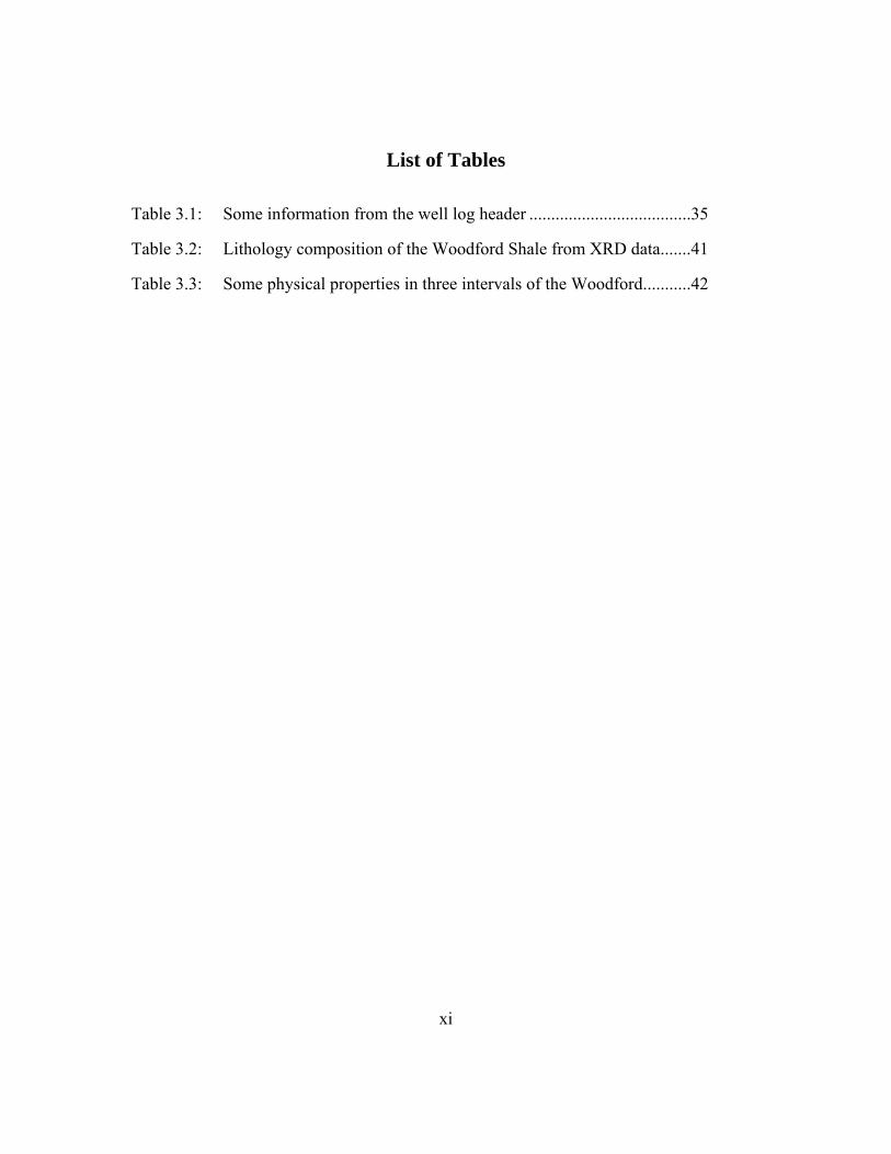
List of Tables

Table 3.1: Some information from the well log header .....................................35

Table 3.2: Lithology composition of the Woodford Shale from XRD data.......41

Table 3.3: Some physical properties in three intervals of the Woodford ...........42

xii

List of Figures

Figure 1.1: Stratigraphy of the Woodford in west Texas and Oklahoma area ......4

Figure 1.2: Outcrop fractures in the Woodford Shale of southeastern

Oklahoma ...........................................................................................6

Figure 1.3: Location of Delaware Basin in west Texas.........................................8

Figure 1.4: Location of Pioneer Reliance Triple Crown borehole (RTC#1) in

Delaware Basin ...................................................................................9

Figure 2.1: Examples of an isotropic medium and three types of anisotropic

media, VTI, HTI and orthorhombic anisotropy ...............................14

Figure 3.1: Basic borehole logs in RTC #1 well .................................................36

Figure 3.2: Three intervals in the Woodford: upper, middle and lower, in the

Permian basin of west Texas and southeast of New Mexico, based

on its log characteristics ...................................................................38

Figure 3.3: Three intervals: upper, middle and lower, in the Woodford of

RTC #1 well. ....................................................................................39

Figure 3.4: ECS log in a zone within the Woodford formation in the RTC #1

borehole.............................................................................................40

Figure 3.5: Vp, Vs, density and Vp/Vs log curves of the Woodford Shale ........43

Figure 3.6: Possible VTI anisotropy in the middle part of the Woodford ...........45

Figure 3.7: Possible HTI anisotropy in the middle layer of the Woodford .........46

Figure 4.1: Seismic modeling using vertical impulsive source, which

generates PP, PS and SS waves .......................................................49

Figure 4.2: Comparison of isotropic and VTI seismic responses for both Z

and X components of PP, PS and SS waves ....................................52

xiii

Figure 4.3: Difference plot between isotropic and VTI models at Z and X

component separately........................................................................53

Figure 4.4: Reflection coefficient sensitivity test for the indicated wave and

component of the VTI model .............................................................55

Figure 4.5: Sensitivity test for VTI case using difference plots ..........................57

Figure 4.6: HTI difference plot at 0 degree azimuth ...........................................59

Figure 4.7: HTI difference plot at 30 degree azimuth .........................................60




Figure 4.11: Crack density sensitivity test for isolated penny-shaped dry

cracks .................................................................................................64

Figure 4.12: Vertical component of HTI seismic model for one shot and

areal grid of receivers geometry ........................................................66

Figure 4.13: The time slices of HTI and isotropic seismic difference for each

component of PP, PS and SS waves before wavefield separation ....68

Figure 4.14: The time slices of HTI and isotropic seismic difference for each

component of PP, PS and SS waves after wavefield separation .......69

Figure 4.15: The time slices of orthorhombic and isotropic seismic difference

for each component of PP, PS and SS waves after wavefield

separation ...........................................................................................70

Figure 5.1: Z (vertical) component of seismic responses to Vp/Vs of 1.54, 1.7

and 2 at thick layers (150m) ...............................................................76

Figure 5.2: X (radial) component of seismic responses to Vp/Vs of 1.54, 1.7

and 2 at thick layers (150m) ...............................................................77

xiv

Figure 5.3: Z (vertical) component of seismic responses to Vp/Vs of 1.54, 1.7

and 2 at actual layer thickness ...........................................................78

Figure 5.4: X (radial) component of seismic responses to Vp/Vs of 1.54, 1.7

and 2 at actual layer thickness ...........................................................79

Figure 5.5: PP reflection coefficient changes with azimuth 0-360 degrees at

different incident angles for matrix background Vp/Vs of 1.54,

1.7 and 2.0 ..........................................................................................81

Figure 5.6: PP reflectivity changes with azimuth, together with Vp versus gas

saturation using Voigt and Reuss average separately ........................84

Figure 5.7: PP reflectivity with azimuthal changes for three matrix background

Vp/Vs ratios at incident angle of 20 degrees and at combination of

water and gas saturation using Voigt average ..................................85

Figure 5.8: PP azimuthal reflectivity for matrix background Vp/Vs of 1.54 at

aspect ratios of 0.1, 0.05 0.01, 0.005 and 0.001 .............................87





Figure 5.11: PP azimuthal reflectivity for matrix background Vp/Vs of 1.54, 1.7

and 2.0 at aspect ratios of 0.1, 0.05, 0.01, 0.005 and 0.001. Gas

saturation is 70% for all curves ........................................................90

1

Chapter 1: Introduction

BACKGROUND OF SHALE GAS PLAYS

Shale is a commonly occurring fine grained clastic sedimentary rock with a mixture

of clay-silt-sized particles. Oil and gas shale, compared to normal shales, contains

kerogen. The kerogen has organic matter and is a potential source of hydrocarbons.

Because of its low permeability that prevents the escape of hydrocarbons, shale is usually

a good seal for a hydrocarbon reservoir. In some cases, shale can also be a good

reservoir, because it can hold a significant amount of hydrocarbons. However, it was not

until recent success in drilling of horizontal wells and production from the Barnett Shale

that the development of unconventional oil and gas shale plays in North America began

to draw considerable attention. Examples of current interest in shale reservoirs include

the Woodford, Antrim, Bakken, Bossier, Marcellus, Eagle Ford and Exshaw Formation.

The shale gas plays have led to a new stage of oil and gas production. The historical

delay of developing shale reservoirs is because the low permeability in the shale prohibits

the gas from being readily released from the source rock. More expensive production

technology, such as hydraulic fracture and horizontal drilling, are needed for these low

permeability reservoirs.

Gas shales are different from tight gas sandstones. Gas shale wells don’t initially

produce as well as tight sandstones, but they can produce consistently for 30 years or

more once production stabilizes (Frantz and Jochen, 2005). Shale reservoirs include

biogenic types, and also thermogenic or combined biogenic-thermogenic gas

accumulations (Curtis, 2002). There are five key parameters that can be used to evaluate

the shale reservoir based on evidence from present producing shale formations: thermal

maturity (expressed as vitrinite reflectance), adsorbed gas fraction, reservoir thickness,

2

total organic carbon content and volume of gas in place (Curtis, 2002). The gas

productivity often relies on the degree of natural fractures and artificial fractures (Curtis,

2002). Dry gas may only be produced from the most thermally mature shales, wetter gas

comes from less thermally mature shales and oil is from the least thermally mature shales

(Frantz and Jochen, 2005). A good shale gas prospect has a shale thickness between 300ft

and 600ft (Frantz and Jochen, 2005).

INTRODUCTION TO THE WOODFORD SHALE

The Woodford Shale is an important unconventional reservoir. It is a hydrocarbon

source rock that acts as a source, seal and reservoir. Late Devonian to Early Mississippian

in age, it extends widely across the mid-continent USA, including parts of Oklahoma,

west Texas and New Mexico (Comer, 1991). Production may come from a range of

lithofacies, including chert, sandstone, dolostone and siltstone, many of which may be

artificially fractured to promote production (Comer, 1991).

1) Lithofacies

The Woodford consists of two main lithofacies, black shale and siltstone (Comer,

1991). Other mixed lithologies, such as sandstone, chert, dolostone, mudstone and light-

colored shale, also exist (Comer, 1991). The lithologies associated with significant

potential gas production are silty black shale in Arkoma Basin in Oklahoma and

Arkansas, chert in the frontal zone of the Ouachita fold belt in Oklahoma, siltstone and

silty black shale in Anadarko Basin in Oklahoma, siltstone and silty black shale in Val

Verde and Midland Basins in Texas, and siltstone and silty black shale in Delaware Basin

in west Texas and New Mexico (Comer, 2007).

2) Stratigraphy and depositional settings

The Woodford is primarily Late Devonian in age, but ranges in age from Middle

3

Devonian to Early Mississippian (Comer, 2008). The stratigraphic column for the

Woodford in west Texas and Oklahoma is shown in Figure 1.1. Note that the

stratigraphic units above and below Woodford are quite different. In west Texas, below

the Woodford is the Thirtyone limestone, while in Oklahoma, the Woodford

unconformably overlies the Hunton group. Above the Woodford is Mississippian Lime.

Ruppel and Loucks (2008) concluded about the Woodford in the Permian Basin, west

Texas: Upper Devonian typically contains abundant biogenic silica, especially in distal

parts of the basin, and the Middle Devonian is dominated by detrital silica. The lower

Woodford was deposited by deep water, turbid flow, whereas the upper Woodford

accumulated under more distal, low energy, poorly oxygenated, hemipelagic conditions

(Ruppel and Loucks, 2008).

3) Source rock and maturity

The Woodford black shale may have high total organic carbon (TOC) as a source

rock. The major oil accumulations of the world typically have TOC content in excess of

2.5 wt% from the source rock (Jones, 1981). The Woodford contains mean organic

carbon concentrations of 4.9% by weight for the Permian Basin (Texas and New

Mexico), 5.7% by weight for the Anadarko Basin (Oklahoma and Arkansas) and 5.2% by

weight for both regions combined (Comer, 2008). These values indicate much higher

TOC content than the sources of many major oil accumulations, which suggest a high

potential as a source of hydrocarbons. The maturity is estimated by measuring the

vitrinite reflectance. The Woodford Shale shows wide range of vitrinite reflectance from

0.7% to 4.89% (Boughal, 2008). In the Arkoma Basin, the thermal maturity is more than

1.15% vitrinite reflectance in dry gas window and less than 1.15% vitrinite reflectance in

oil window (Cardott, 2008). In the Anadarko Basin, from northeast to southwest, the

average vitrinite reflectance increases from 0.51% to 2.6%, showing an increasing trend

Figure 1.1: Stratigraphy of the Woodford in west Texas and Oklahoma area. On the left

shows the Delaware Basin (Ali, 2009, modified from Dutton et al., 2005) of west Texas

and on the right shows the Anardako Basin in Oklahoma (Wang and Philp, 1997).

4

5

of thermal maturity (Lambert, 1982).

4) Fractures

The Woodford may contain natural fractures due to its mechanical properties (such as

high brittleness), overburden stress and its geologic settings (such as near a fault). Portas

and Slatt (2010) studied the fracture patterns in a Woodford Shale exposure in a quarry in

southeastern Oklahoma using the outcrop descriptions and LIDAR data, and found that

there is a great abundance of fractures in the upper Woodford. Another study (Andrews,

2009) on the outcrops of southeast Oklahoma also indicated the existence of natural

fractures (Figure 1.2). Figure 1.2a shows interbedded cherty and shale beds, where the

fractures exist widely perpendicular to the bedding but die out in the bounding shale.

Figure 1.2b illustrates the black to grey fissile shale.

5) Production

The Woodford may contain both natural fractures and quartz rich sections. It may be

brittle enough to generate induced fractures using hydraulic fracturing techniques. In the

Permian Basin of west Texas, the upper Woodford contains quartz rich rocks and

responds positively to fractures during the hydraulic fracturing completion; and the

brittleness, characterized by Young’s modulus and Poisson’s ratio, is high (Aoudia et al.,

2009). Production activity in the Woodford began in 2003-2004 with conventional

(vertical) drilling (Boughal, 2008). Fractures (natural and induced) are the pathways for

gas and oil to migrate to the borehole. Since 2005, about 1000 Woodford wells have been

put into production in Oklahoma, with over half of these drilled in 2008 (Boyd, 2009).

Total production through 2009 is 450MMCFPD (Boyd, 2009). In west Texas and

southeastern New Mexico, estimates for the potential of the Woodford Shale are on the

order of 80 billion bbl of oil (240 trillion cubic feet of natural gas equivalent) (Comer,

1991).

a: cherty beds are highly fractured perpendicular to bedding but die out in the bounding

shale.

Cherty bed

Shale

Cherty bed

Shale

Cherty bed

b: black to gray fissile shale.

Figure 1.2: Outcrop fractures in the Woodford Shale of southeastern Oklahoma (modified

from Andrews, 2009).

6

7

DATA

The borehole data for this Woodford study come from well logs in one borehole in

the Delaware Basin (Pecos County), west Texas. The well data include standard log

suites: sonic, gamma ray, resistivity, density, neutron porosity dipole sonic logs, a small

interval of imaging (FMI) logs and also elemental capture spectroscopy (ECS) and X-ray

diffraction (XRD) data from core samples. The log includes many formations (e.g.

Morrow sand, Atoka sand, Barnett, Mississippian Lime, and Woodford).

Figure 1.3 shows the location of Delaware Basin in west Texas (modified from Ali,

2009; King, 1942; Brown, 2007). The Delaware Basin is surrounded by the Northwest

Shelf, Central Basin Uplift and Diablo Platform. To the south is the Marathon Collision

Zone. The Central Basin Uplift separates the Delaware Basin from the Midland Basin.

The well used for this study, the Pioneer Resources Reliance Triple Crown #1 (RTC

#1), was drilled in Pecos County of Texas, in the southern part of Delaware Basin (Figure

1.4). It is located in an area that was 600ft deep during the Late Devonian (Ali, 2009;

Gutschick and Sandberg, 1983).

The Woodford Shale in Delaware Basin is of the late Devonian to early Mississippian

age. It is overlain by Mississippian lime and the Barnett Shale, and unconformably

underlain by the Thirtyone formation (Dutton et al., 2005). In the RTC #1 well, the

Mississippian Lime above the Woodford Shale is actually chert mixed with dolomite

(Ali, 2009).

OBJECTIVES

The objective of this study is to use the well log data as a basis to numerically

simulate the seismic response to various models of potentially productive conditions in

N

Figure 1.3: Location of Delaware Basin in west Texas (modified from Ali, 2009; King,

1942; Brown, 2007). The Delaware Basin is surrounded by Northwest Shelf, Central

Basin Uplift and Diablo Platform.

8

Figure 1.4: Location of Pioneer Reliance Triple Crown borehole (RTC #1) in Delaware

Basin (modified from Ali, 2009), showing the distribution of Mississippian wells (red,

blue and yellow dots). RTC #1 well (black dot) is in the southern part of Delaware Basin.

9

10

the Woodford interval. Rock physics analysis followed by seismic simulation (modeling)

is a useful tool to link well logs with surface seismic reflection data. Through rock

physics modeling, appropriate parameters are identified to simulate the seismic response,

which may be a good basis for analyzing the surface seismic record. This study is

designed to test the sensitivities to variations of different elastic constants in the

Woodford Shale to different rock conditions—basically evaluating variations in internal

anisotropy. Anisotropy may be an important parameter associated with source, seal and

reservoir conditions. For example, Vernik and Liu (1997) found that the anisotropy

parameter ε increases with kerogen content until it reaches the maximum value of 0.4.

Anisotropy may also associate with fracturing production and borehole completion. The

natural fractures (e.g. presented in terms of horizontal or vertical fractures) in the rock

may provide a pathway for the oil and gas to migrate to the producing borehole.

In this study, a single borehole log does not have enough information about the

anisotropy in the Woodford to fully describe rock physics properties. In order to test the

anisotropic seismic response, I mainly address three types of anisotropy: transversely

isotropic with a vertical symmetry axis (VTI), transversely isotropic with a horizontal

symmetry axis (HTI) and orthorhombic anisotropy, together with an isotropic model.

These various scenarios predict corresponding seismic responses. By changing the

anisotropy parameters, I test the sensitivity of the seismic response (particularly

variations in reflection amplitude with source-receiver offset, AVO) in synthetic seismic

data to variations in the middle unit of the Woodford. These AVO variations are also

considered for different wave types, P-P, P-SV and SV-SV waves. I found that the

sensitivity to AVO variations not only depends on the type of anisotropy and anisotropy

parameters, but also on the rock matrix properties such as matrix background velocities

(Vp/Vs ratio), density, and fluid saturation. Obtaining a better understanding of what

11

affects the seismic response in the Woodford will help develop techniques to work on the

surface reflection seismic data.

THESIS ORGANIZATION

The thesis is divided into five chapters. Chapter 1 provides a brief overview of the

Woodford Shale featured in North America and introduction of the Woodford in the

study area. Chapter 2 introduces the theories and methods of anisotropy. The theories in

chapter 2 provide the key background for understanding the study presented in the

following chapters. Chapters 3, 4 and 5 constitute the body of this thesis, which explore

building models to different anisotropic scenarios. Chapter 6 contains the discussions and

conclusions for all the work done in this thesis.

Chapter 3 describes the log and borehole characteristics of Woodford Shale, based on

the observations from the well logs. The description includes gamma ray, resistivity,

density, P wave and S wave velocity (sonic and dipole sonic logs), and lithology

properties in the Woodford interval. After examining the log data, I divide the Woodford

into three intervals: upper, middle and lower. Meanwhile, by examining the gamma ray

response, I find there is possible VTI anisotropy in the middle Woodford; and by

examining the dipole shear log and a part of FMI data, I discover that possible HTI

anisotropy can exist in the middle Woodford as well. However, there is no sufficient

evidence to prove the existence of these types of anisotropy in the Woodford. Modeling

is conducted based on assumptions.

Based on the log division and characteristics stated in chapter 3, chapter 4 explores

the change of simulated seismic response to different kinds of anisotropy in the middle

Woodford. Isotropic and VTI models have been created first to compare with each other

and test VTI parameters; then isotropic and dry HTI models have been made to see the

12

difference between the two models and test HTI parameters; last, the orthorhombic model

is tested to see the difference.

Chapter 5 is an extension to chapter 4, which explores the sensitivity test on the

middle Woodford for HTI model. The matrix background Vp/Vs ratio (mainly Vp

changes) is an important factor for the sensitivity analysis. Together with the fluid

saturation and aspect ratio, a comprehensive seismic response appears with the azimuthal

amplitude change. These factors are a guide for further field analysis.

Chapter 6 is the discussions and conclusions to the whole thesis.

13

Chapter 2: Fundamentals of Anisotropy

The goals of this chapter are to:

1) Introduce the basics of anisotropy descriptions and how various types of

anisotropy impact seismic wave propagation.

2) Understand VTI and its representation using Thomsen (1986) parameters.

3) Understand HTI and its model parameters. I use two rock physics models to

describe anisotropy: one is the Hudson (1980, 1981) model, the other is Bakulin

et al. (2000, part I) model.

4) Understand orthorhombic anisotropy parameters (Tsvankin, 1997; Bakulin et al.,

2000, part II).

5) Understand how anisotropy can affect the AVO response of P-P, P-SV and SV-

SV reflections and the entire seismic reflection processes.

INTRODUCTION TO ANISOTROPY

The seismic propagation velocity in isotropic media does not vary with either

polarization or propagation directions, but the velocity does often vary significantly with

propagation and polarization directions for the anisotropic media. Figure 2.1 shows

examples of an isotropic model and three common anisotropic models. An isotropic

medium is totally symmetric; a transversely isotropic with a vertical symmetry axis (VTI)

medium has a characteristic of horizontal stratified thin layers, which are very common

during geologic sedimentation; a transversely isotropic with a horizontal symmetry axis

(HTI) medium has a characteristic of vertical fractures, which are often seen in fractured

carbonate or the area near faults; an orthorhombic medium has two symmetry axes, one is

Isotropic

VTI

HTI

Orthorhombic

X3

X1

X1

X3X2

Figure 2.1: Examples of an isotropic medium and three types of anisotropic media, VTI,

HTI and orthorhombic anisotropy.

14

horizontal and the other is vertical. Orthorhombic anisotropy may be formed by

combination of vertical and horizontal fractures or by vertical fractures added into a VTI

background, which may be seen in layered media or laminated shale with natural or

induced vertical fractures.

According to Hooke’s law, for effective media with linear elastic solid properties, the

stress is proportional to the strain and can be expressed by: ij ijkl klCσ ε= , (2.1)

where ijσ is stress tensor, klε is strain tensor and is stiffness matrix. (a

fourth-ranked matrix) has 81 components, but due to the symmetry conditions of the

stress and strain tensors, it is reduced to 21 components. This reduction leads to the

reformulation of the stress (T) and strain (E) in the follows:

ijklC ijklC

1 11

2 22

3 23

4 23

5 13

6 12

T

σ σσ σσ σσ σσ σσ σ

=⎡ ⎤⎢ ⎥=⎢ ⎥⎢ ⎥=

= ⎢ =⎢ ⎥⎢ ⎥=⎢ ⎥

=⎢ ⎥⎣ ⎦

⎥

1 11

2 22

1 33

4 23

5 13

6 12

222

eee

Eeee

εεεεεε

=⎡ ⎤⎢ ⎥=⎢ ⎥⎢ ⎥=

= ⎢ ⎥=⎢ ⎥⎢ ⎥=⎢ ⎥

=⎢ ⎥⎣ ⎦ .

Then the subscripts of stiffness matrix can be replaced i(j) by in each pair

of indices ij (kl) with the relations below:

ijklC ij ijklc C=

ij (kl) i (j)

11 1

22 2

33 3

23, 32 4

13, 31 5

12, 21 6

15

In this way, (6, 6) is substituted for (3, 3, 3, 3). The stiffness matrix is thus

restated as a 6x6 matrix. (Mavko et al., 2003). The stiffness matrix is expressed as

follows with different anisotropy type:

ijc ijklC

ijc

1) Isotropic media

16

⎥

,

(2.2)

11 12 12

12 11 12

12 12 11

44

44

44

0 0 00 0 00 0 0

0 0 0 0 00 0 0 0 00 0 0 0 0

ij

c c cc c cc c c

cc

cc

⎡ ⎤⎢ ⎥⎢ ⎥⎢ ⎥

= ⎢⎢ ⎥⎢ ⎥⎢ ⎥⎢ ⎥⎣ ⎦

here , it has a total of two independent constants. 12 11 442c c c= − 2) VTI and HTI media

Figure 2.1 shows the configurations of VTI and HTI anisotropic models, where

the symmetry axis of VTI model is in the 3x direction and the symmetry axis of

HTI model is in the 1x direction. The stiffness matrices of VTI and HTI media

can be written as comparison in the following equations (Ruger, 2002):

11 12 13

12 11 13

13 13 33

55

55

66

0 0 00 0 00 0 0

( )0 0 0 0 00 0 0 0 00 0 0 0 0

ij

c c cc c cc c c

c VTIc

cc

⎡ ⎤⎢ ⎥⎢ ⎥⎢ ⎥

= ⎢ ⎥⎢ ⎥⎢ ⎥⎢ ⎥⎢ ⎥⎣ ⎦ ,

(2.3)

here , it has 5 independent constants. 12 11 662c c c= −

11 13 13

13 33 23

13 23 33

44

55

55

0 0 00 0 00 0 0

( )0 0 0 0 00 0 0 0 00 0 0 0 0

ij

c c cc c cc c c

c HTIc

cc

⎡ ⎤⎢ ⎥⎢ ⎥⎢ ⎥

= ⎢ ⎥⎢ ⎥⎢ ⎥⎢ ⎥⎢ ⎥⎣ ⎦ ,

(2.4)

here , it has 5 independent constants. 23 33 442c c c= −

3) Orthorhombic media

11 12 13

12 22 23

13 23 33

44

55

66

0 0 00 0 00 0 0

( )0 0 0 0 00 0 0 0 00 0 0 0 0

ij

c c cc c cc c c

c orc

cc

⎡ ⎤⎢ ⎥⎢ ⎥⎢ ⎥

= ⎢ ⎥⎢ ⎥⎢ ⎥⎢ ⎥⎢ ⎥⎣ ⎦ ,

(2.5)

it has 9 independent constants.

ELASTIC MEDIA

1) Isotropic media

17

The term isotropic is different from the term homogeneous. In homogenous media,

the composition or structure of elements is distributed uniformly. Homogenous media can

be isotropic and isotropic media can be homogenous. In isotropic media as Figure 2.1

shows, velocity does not depend on direction. That is, velocity is constant whatever the

propagation or polarization direction of the wave is. Understanding the reflection,

transmission and mode conversion in isotropic media through the Zoeppritz equations

(Zoeppritz, 1919) is a key to understand the seismic propagation. Based on that, recent

researchers (Aki and Richards, 1980; Shuey, 1985; Hilterman, 1989; Thomsen, 1990)

give the linear approximation forms of PP wave reflection amplitude versus offset (AVO)

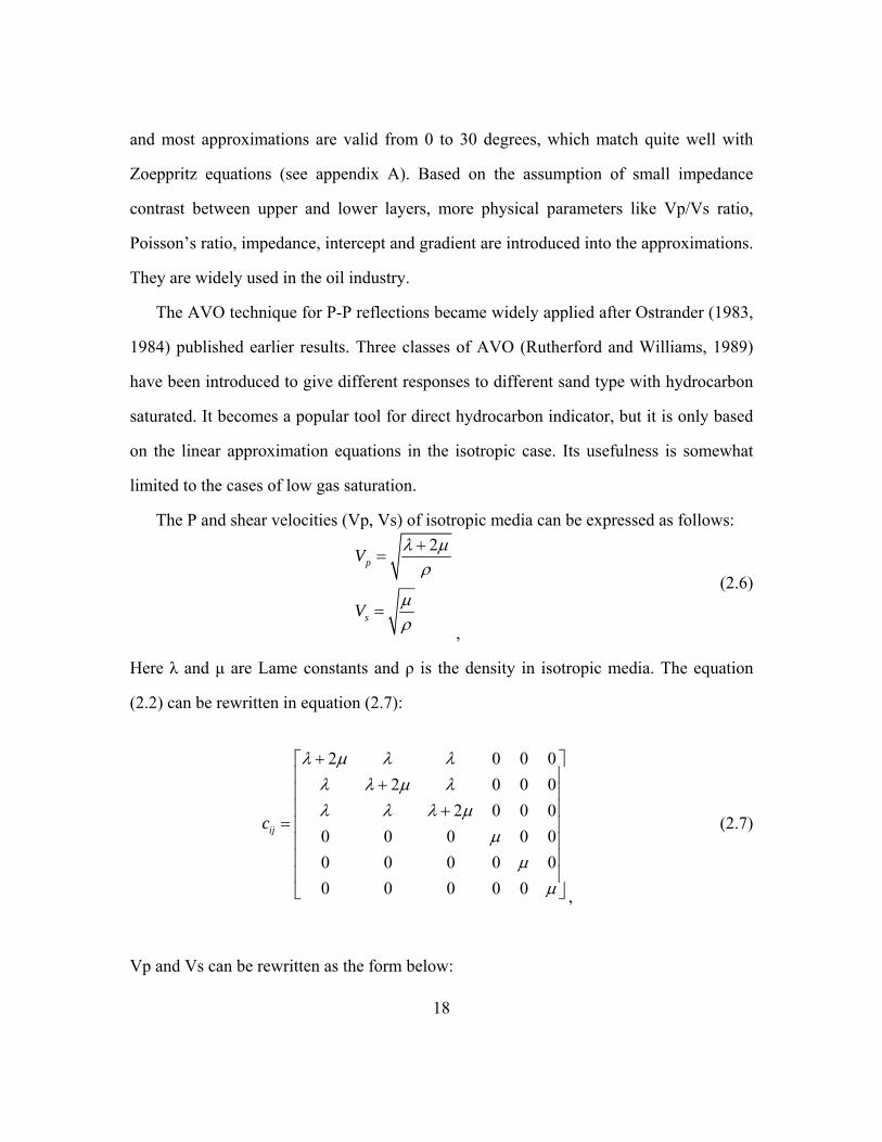
and most approximations are valid from 0 to 30 degrees, which match quite well with

Zoeppritz equations (see appendix A). Based on the assumption of small impedance

contrast between upper and lower layers, more physical parameters like Vp/Vs ratio,

Poisson’s ratio, impedance, intercept and gradient are introduced into the approximations.

They are widely used in the oil industry.

The AVO technique for P-P reflections became widely applied after Ostrander (1983,

1984) published earlier results. Three classes of AVO (Rutherford and Williams, 1989)

have been introduced to give different responses to different sand type with hydrocarbon

saturated. It becomes a popular tool for direct hydrocarbon indicator, but it is only based

on the linear approximation equations in the isotropic case. Its usefulness is somewhat

limited to the cases of low gas saturation.

The P and shear velocities (Vp, Vs) of isotropic media can be expressed as follows:

2p

s

V

V

λ μρ

μρ

+=

=,

(2.6)

Here λ and μ are Lame constants and ρ is the density in isotropic media. The equation

(2.2) can be rewritten in equation (2.7):

2 0

2 0 02 0 0 0

0 0 0 00 0 0 00 0 0 0 0

ijc

λ μ λ λλ λ μ λλ λ λ μ

μμ

0 00

00μ

+⎡ ⎤⎢ ⎥+⎢ ⎥⎢ ⎥+

= ⎢ ⎥⎢ ⎥⎢ ⎥⎢ ⎥⎣ ⎦ ,

(2.7)

Vp and Vs can be rewritten as the form below:

18

11

5544

p

s

cV

ccV

ρ

ρ ρ

=

= =.

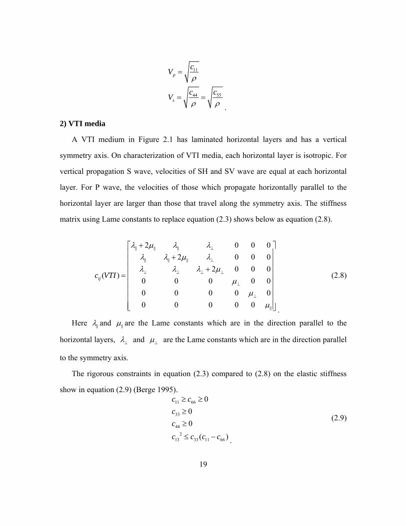
2) VTI media

A VTI medium in Figure 2.1 has laminated horizontal layers and has a vertical

symmetry axis. On characterization of VTI media, each horizontal layer is isotropic. For

vertical propagation S wave, velocities of SH and SV wave are equal at each horizontal

layer. For P wave, the velocities of those which propagate horizontally parallel to the

horizontal layer are larger than those that travel along the symmetry axis. The stiffness

matrix using Lame constants to replace equation (2.3) shows below as equation (2.8).

2 02 0 0

2 0 0 0( )

0 0 0 00 0 0 00 0 0 0 0

ijc VTI


μμ

0 00

00μ

⊥

⊥

⊥ ⊥ ⊥ ⊥

⊥

⊥

+⎡ ⎤⎢ ⎥+⎢ ⎥⎢ ⎥+

= ⎢ ⎥⎢ ⎥⎢ ⎥⎢ ⎥⎢ ⎥⎣ ⎦ .

(2.8)

Here λ and μ are the Lame constants which are in the direction parallel to the

horizontal layers, λ⊥ and μ⊥ are the Lame constants which are in the direction parallel

to the symmetry axis.

The rigorous constraints in equation (2.3) compared to (2.8) on the elastic stiffness

show in equation (2.9) (Berge 1995). 11 66

33

442

13 33 11 66

000

( )

c ccc

c c c c

≥ ≥

≥≥

≤ − .

(2.9)

19

Backus (1962) demonstrated that for finely layered, horizontally stratified,

transversely isotropic elastic media, for seismic wavelength larger than the layer

thickness, the elastic constants of each horizontal layer could be averaged to represent an

anisotropic medium as a single homogeneous medium. For this kind of anisotropy,

additional constraints are applied in equation (2.10) (Backus, 1962; Berge 1995).

33 13

33 44

66 44

43

c c

c c

c c

>

>

≥ .

(2.10)

Thomsen (1986) pointed out the concept of weak elastic anisotropy, which exists in

most bulk elastic media (10-20 percent of the media summarized from earlier papers). He

derived the parameters ε, γ and δ known as Thomsen’s parameters that are expressed as

elastic constants in equation (2.11), which have more physical meanings.

33

55

11 33

33

66 44

442 2

13 44 33 44

33 33 44

2

2

( ) (2 ( )

cVp

cVs

Vp Vpc cc Vp

Vs Vsc cc Vs

c c c cc c c

ρ

ρ

ε

γ

δ

⊥

⊥

⊥

⊥

⊥

⊥

=

=

−−= ≈

−−= ≈

+ − −=

−)

.

(2.11)

Here Vp and are the P wave velocity and S wave velocity respectively

traveling along the symmetry axis. Vp is the P wave propagating orthogonal to the

vertical symmetry axis. is the fast shear wave velocity traveling along the horizontal

layer and polarizing along the horizontal layer, and

⊥ Vs⊥

Vs

Vs⊥ is the slow shear wave velocity,

that propagates along the vertical symmetry axis but polarizes along the horizontal layer.

20

Compared with equations (2.8), (2.3) and (2.6), ε is expressed as the degree of P wave

anisotropy, due to the difference between and , or Vp and Vp . We know

from equation (2.8) that represents the P wave velocity parallel to the horizontal

layers and shows the P wave velocity parallel to the symmetry axis. γ is expressed as

the degree of S wave anisotropy. For weak anisotropy, Thomsen also pointed out that δ

controls most important anisotropic phenomena in exploration geophysics. And it

controls the near vertical P wave propagation. For weak anisotropy, ε, γ and δ <<1. He

summarized measured anisotropy in sedimentary rock from many researchers and

concluded that most of these rocks have anisotropy in the weak-to-moderate range (<0.2).

11c 33c ⊥

11c

33c

For the intrinsic case, the elliptically anisotropic media have the character δ=ε (Daley

and Hron, 1979; Thomsen, 1986). If anisotropy is caused by fine layering of isotropic

materials, δ<ε (Berryman, 1979; Helbig, 1979; Thomsen, 1986). According to equations

(2.3), (2.8), (2.9) and (2.10), it is not hard to find that ε>0 and γ>0 in VTI media. δ can be

either positive or negative.

3) HTI media

a) Equivalent Thomsen’s parameters

An HTI medium in Figure 2.1 has vertical fractures and a horizontal symmetry axis.

Fractures can cause shear wave splitting. SV and SH waves which propagate downward

in the vertical plane do not have the same velocity any more. The horizontally polarized

SH wave (in the isotropic plane) travels faster than the vertically polarized SV wave (in

the vertical plane). Specially for the fractures which are not oriented vertically, the

splitting generates two waves. One is called fast shear wave (S1), which polarizes parallel

to the fractures; the other is called slow shear wave (S2), which polarizes perpendicular

to the fractures. For P wave travelling vertically in Figure 2.1, it travels along the vertical

21

22

0 00

00

isotropic plane and its velocity is larger than that propagates along the symmetry axis.

The stiffness matrix using Lame constants can be derived from equation (2.4) as below. 2 0

2 0 02 0 0 0

( )0 0 0 00 0 0 00 0 0 0 0

ijc HTI


μμ

μ

⊥ ⊥ ⊥ ⊥

⊥

⊥

⊥

⊥

+⎡ ⎤⎢ ⎥+⎢ ⎥⎢ ⎥+

= ⎢ ⎥⎢ ⎥⎢ ⎥⎢ ⎥⎢ ⎥⎣ ⎦ .

(2.12)

Here λ and μ are the Lame constants which are in the direction parallel to the

vertical fractures, λ⊥ and μ⊥ are the Lame constants which are in the direction

perpendicular to the factures.

Similar anisotropy parameters in equation (2.11) have been derived to represent the

physical meanings for HTI media (Ruger, 1995, 1996; Chen, 1995; Mavko et al., 2003).

33

44

55

( ) 11 33

33

( ) 66 44

44

2 2( ) 13 55 33 55

33 33 55

2

2

( ) (2 ( )

v

v

v

cVp

cVs

cVs

Vp Vpc cc Vp

Vs Vsc cc Vs

c c c cc c c

ρ

ρ

ρ

ε

γ

δ

⊥

⊥

⊥

=

=

=

−−= ≈

−−= ≈

+ − −=

−)

.

(2.13)

Here and are the P wave velocity and S wave velocity respectively

traveling along the vertical fractures. is the S wave polarized in the vertical isotropic

plane traveling in the vertical direction and Vs

Vp Vs

Vs

⊥ is the S wave polarized along the

symmetry axis traveling vertically. ( )vε and ( )vγ express as the degree of anisotropy for

P wave and S wave, just similar as described in VTI Thomsen’s parameters. Comparing

equation (2.4) with (2.12), the elastic constants parallel to the fractures are larger than

that perpendicular to the fractures. Thus, it is not difficult to find out that ( )vε and ( )vγ are both negative. ( )vδ can be either positive or negative. The HTI parameters can be

related to the Thomsen’s parameters in the VTI media as below (Ruger, 2002): ( )

( )

( )

20

0

1 2

1 2

2 (1 )

2(1 2 )(1 )

1 ( )

v

v

v

S

P

f

fVfV

εεε

γγγ

εδ εδ εε

= −+

= −+

− +=

+ +

= −.

(2.14)

Here and 0SV 0PV are measured along the horizontal axis. ε , γ and β are Thomsen’s

parameters discussed in equation (2.11). The HTI parameters should also be: ( )vε , ( )vγ and ( )vδ <<1.

b) Hudson’s Model for cracked media

Hudson (1980, 1981) introduced a fracture model with isolated penny-shaped

inclusions (cracks). Cases of “cracks” include random and single orientations. The

seismic wavelength should be much longer than the scale length of the inclusions. Crack

density in Hudson’s theory is related to number of inclusions per unit volume (equation

2.15) (Hudson, 1980; Mavko et al., 2003). This means the larger the crack density, the

more inclusions in the model. When the crack density approaches a limit, the inclusions

interact; therefore, the rock will fall apart. In Hudson’s theory, the crack density is

limited to a maximum value of 0.1 to be valid. Aspect ratio in this theory is defined as the

23

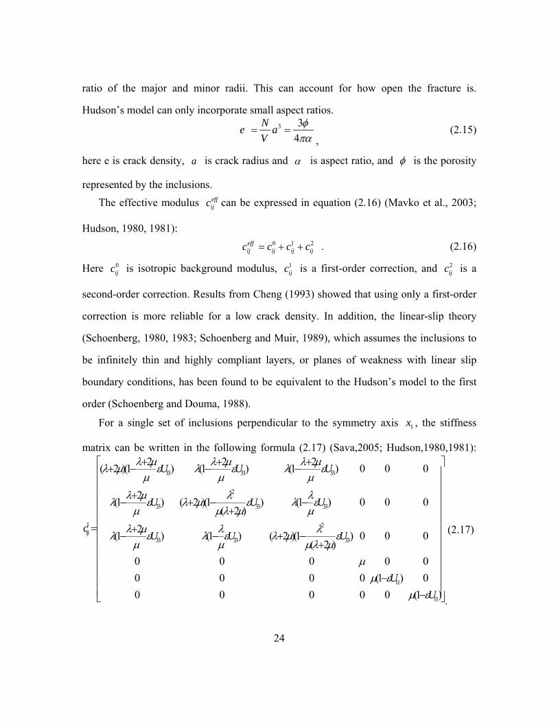
ratio of the major and minor radii. This can account for how open the fracture is.

Hudson’s model can only incorporate small aspect ratios. 3 3

4Ne aV

φπα

= =, (2.15)

here e is crack density, is crack radius and a α is aspect ratio, and φ is the porosity

represented by the inclusions. The effective modulus can be expressed in equation (2.16) (Mavko et al., 2003;

Hudson, 1980, 1981):

effijc

0 1effij ij ij ijc c c c2= + + . (2.16)

Here is isotropic background modulus, is a first-order correction, and is a

second-order correction. Results from Cheng (1993) showed that using only a first-order

correction is more reliable for a low crack density. In addition, the linear-slip theory

(Schoenberg, 1980, 1983; Schoenberg and Muir, 1989), which assumes the inclusions to

be infinitely thin and highly compliant layers, or planes of weakness with linear slip

boundary conditions, has been found to be equivalent to the Hudson’s model to the first

order (Schoenberg and Douma, 1988).

0ijc 1

ijc 2ijc

For a single set of inclusions perpendicular to the symmetry axis 1x , the stiffness

matrix can be written in the following formula (2.17) (Sava,2005; Hudson,1980,1981):

33 33 33

2

33 33 33

1 2

33 33 33

11

11

2 2 2( 2 )(1 ) (1 ) (1 ) 0 0 0

2(1 ) ( 2 )(1 ) (1 ) 0 0 0( 2 )

2(1 ) (1 ) ( 2 )(1 ) 0 0 0( 2 )

0 0 0 00 0 0

01 ) 0

0 0 0 0 (1 )

ij

U U U

U U U

cU U U

UU

λ μ λ μ λ μλ μ ε λ ε λ εμ μ μ

λ μ λ λλ ε λ μ ε λ εμ μλ μ μ

λ μ λ λλ ε λ ε λ μ εμ μ μλ μ

μμ ε

μ ε

+ + +⎡ + − − −⎢⎢⎢ +

− + − −⎢ +⎢⎢= +

− − + −⎢+

−−⎣

⎤⎥⎥⎥⎥⎥⎥⎥

⎢ ⎥⎢ ⎥⎢ ⎥⎢ ⎥⎢ ⎥⎦

0 (0 .

(2.17)

24

Here, and depend on the crack conditions: 33U 11U

11

33

16( 2 )3(3 4 )(1 )

4( 2 )3( )(1 )

UM

Uk

λ μλ μλ μ

λ μ

+=

+ ++

=+ + .

(2.18)

Here, '

' '

4 ( 2 )( )4( )( 23

( )

M

Kk

μ λ μπαμ λ μ

)μ λ μ

παμ λ μ

+=

+

+ +=

+ ,

(2.19)

'K is the bulk modulus of the inclusion material and 'μ is the shear modulus of the

inclusions, λ and μ are the Lame constants under the condition of isotropic rock matrix

and α is the aspect ratio. Using equation (2.19), the elastic constants of the different

fluid saturation in the inclusions can be calculated. For dry cracks when M and k equal

zero, we can get:

11

33

16( 2 )3(3 4 )4( 2 )3( )

U

U

λ μλ μλ μλ μ

+=

++

=+ .

(2.20)

For using Hudson’s model to the first order, crack density and aspect ratio must be

small. The crack density should be smaller than 0.1, and the aspect ratio should be

smaller than 0.3 (Sava, 2005). The Eshelby-Cheng model (Mavko et al., 2003; Cheng,

1978, 1993; Eshelby, 1957) has low crack concentrations but can have large aspect ratio.

Hudson (1986) also derived the formula with second order in crack density by the method

of smoothing, extended to the case where the cracks consist of two or more sets of

fractures that are aligned in different directions.

25

This model is valid for high frequency conditions; if used in low frequency case,

Brown and Korringa (1975) relations should be used to saturate fluid content (Mavko et

al., 2003).

c) Bakulin’s Model

Hudson’s model in equations (2.17) and (2.18) can be used to calculate the elastic

constants of the bulk material in the case of different amount of fluid saturation. Bakulin

et al. (2000, part I) derived the explicit expressions for dry and fluid-filled cracks from

Hudson’s model under the condition of isolated penny-shaped cracks. He obtained the

HTI parameters as a function of the crack density and the Vs/Vp ratio for cracks that are

either dry or fluid saturated. No intermediate saturation is allowed. For dry (or gas-filled)

cracks, the anisotropy parameters are:

( )

( )

( )

( )

838 (1 2 )13 (3 2 )(1 )

83(3 2 )

8 (1 2 )3 (3 2 )(1 )

v

v

v

v

e

g geg g

eg

g geg g

ε

δ

γ

η

= −

⎡ ⎤−= − +⎢ ⎥− −⎣ ⎦

= −−

⎡ ⎤−= ⎢ ⎥− −⎣ ⎦ .

(2.21)

Here e is the crack density, , Vs and Vp are calculated from isotropic rock

matrix and

2( / )g Vs Vp=

( )vη is the degree of anellipticity (Tsvankin, 1997): ( ) ( )

( )( )1 2

v vv

v

ε δηδ−

=+ .

(2.22)

Vp/Vs ratio is generally above 1.4. When Vp/Vs is 2 (about 1.4), the Poisson’s ratio

becomes zero, which is not very likely in rocks. So generally, g<0.5. Then we can obtain: ( )( ) ( )0, 0, 0vv vε δ γ≤ ≤ ≤ . (2.23)

26

If we assume1. , which is a quite common range for most sedimentary

rock, we obtain 0.12 ; then the corresponding ranges of coefficients in

equation (2.21) are:

5 / 2.86Vp Vs≤ ≤

0.42g≤ ≤

( )

( )

( )

( )

2.68( 2.82 0.05)

( 1.10 0.13)(0.14 0.05)

v

v

v

v

ee

ee

ε

δ

γ

η

= −

= − ±

= − ±

= ± .

(2.24)

27

0≈

From equation (2.24), the HTI media with dry cracks have the relationships

, which represent elliptically anisotropy. These parameters largely

depend on crack density, but they do not rely on g significantly. This also verifies the

discovery

( ) ( ) ( ),v v vε δ η≈

( )| |v eγ ≈ (Thomsen, 1995; Tsvankin, 1997). For the case of fluid-filled cracks,

equation (2.21) changes to equation (2.25).

( )

( )

( )

( )

032

3(3 2 )8

3(3 2 )32

3(3 2 )

v

v

v

v

geg

eg

geg

ε

δ

γ

η

=

= −−

= −−

=− ,

(2.25)

( )vε represents the P-wave anisotropy and becomes zero when saturated with fluid. The

shear anisotropy coefficient ( )vγ is the same as that in equation (2.21), because fluid

does not affect the property of shear modulus. Fluid can change the values of ( )vδ and ( )vε .

The models discussed here are only applicable to a single fluid saturation.

Combinations of fluid saturation should be addressed using Hudson’s model. In spite of

the limitations, this is a straightforward way to test the seismic response of fractured rock

by using only few physical parameters.

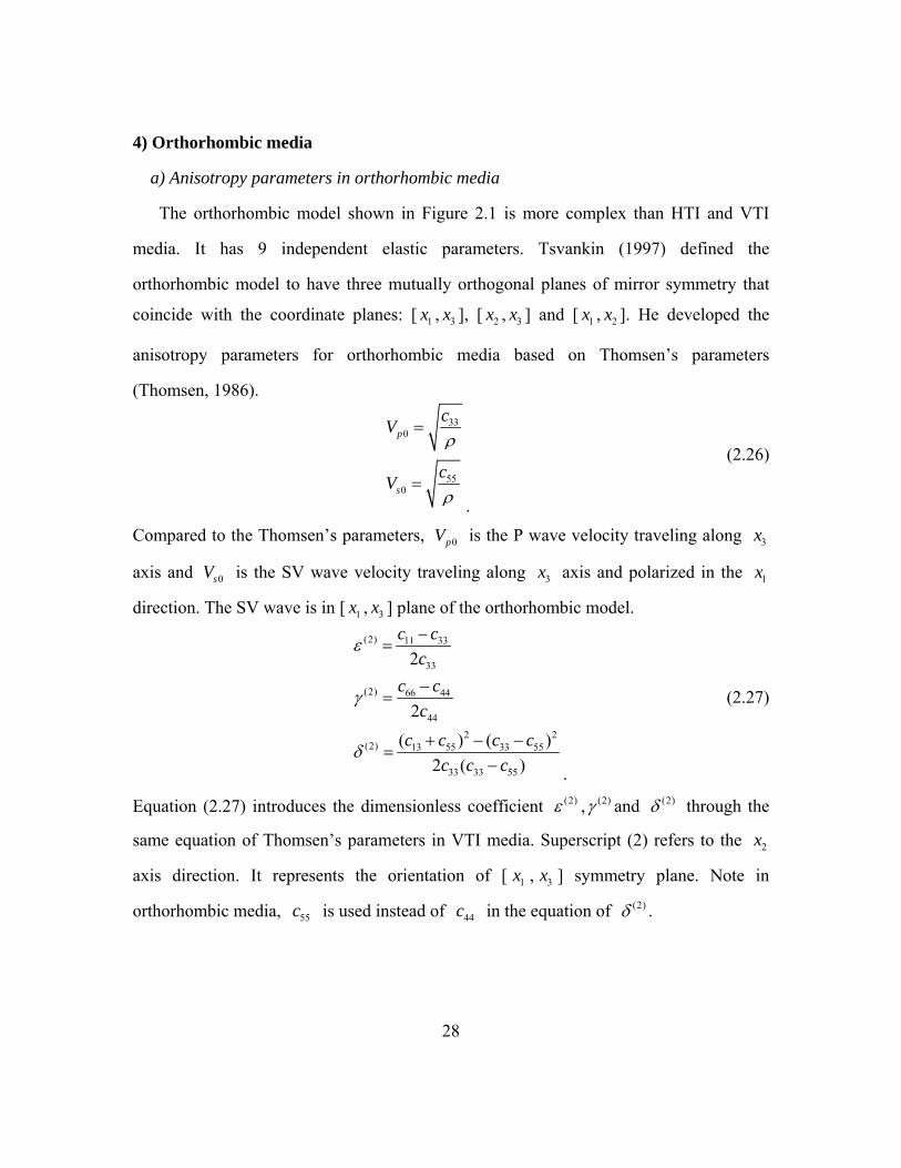
4) Orthorhombic media

a) Anisotropy parameters in orthorhombic media

The orthorhombic model shown in Figure 2.1 is more complex than HTI and VTI

media. It has 9 independent elastic parameters. Tsvankin (1997) defined the

orthorhombic model to have three mutually orthogonal planes of mirror symmetry that

coincide with the coordinate planes: [ 1x , 3x ], [ 2x , 3x ] and [ 1x , 2x ]. He developed the

anisotropy parameters for orthorhombic media based on Thomsen’s parameters

(Thomsen, 1986).

330

550

p

s

cV

cV

ρ

ρ

=

=.

(2.26)

Compared to the Thomsen’s parameters, is the P wave velocity traveling along 0pV 3x axis and 0sV is the SV wave velocity traveling along 3x axis and polarized in the 1x direction. The SV wave is in [ 1x , 3x ] plane of the orthorhombic model.

(2) 11 33

33

(2) 66 44

442 2

(2) 13 55 33 55

33 33 55

2

2

( ) (2 ( )

c cc

c cc

c c c cc c c

ε

γ

δ )

−=

−=

+ − −=

− .

(2.27)

Equation (2.27) introduces the dimensionless coefficient (2)ε , (2)γ and (2)δ through the

same equation of Thomsen’s parameters in VTI media. Superscript (2) refers to the 2x

axis direction. It represents the orientation of [ 1x , 3x ] symmetry plane. Note in

orthorhombic media, is used instead of in the equation of 55c 44c (2)δ .

28

(1) 22 33

33

(1) 66 55

552 2

(1) 23 44 33 44

33 33 44

2

2

( ) (2 ( )

c cc

c cc

c c c cc c c

ε

γ

δ )

−=

−=

+ − −=

− .

(2.28)

Equation (2.28) introduces the parameters (1)ε , (1)γ and (1)δ defined similar to (2)ε , (2)γ and (2)δ in equation (2.27). These describe the anisotropy of P and S wave in

[ ]2 , 3x x plane normal to 1x axis. Equations (2.27) and (2.28) include eight elastic

parameters but only missing . 12c (3)δ is introduced to include . 12c

2 2

(3) 12 66 11 66

11 11 66

( ) (2 ( )

c c c cc c c

δ + − −=

−)

, (2.29)

(3)δ above is the VTI parameter δ in the [ ]1 2,x x plane with 1x to be the symmetry

axis instead of 3x .

Equations (2.26) to (2.29) can describe the anisotropy in orthorhombic media. In

particular, the orthorhombic model reduces to VTI when: (2) (1)

(2) (1)

(2) (1)

(3) 0

ε ε ε

γ γ γ

δ δ δ

δ

= =

= =

= =

= .

(2.30)

b) Orthorhombic model

Bakulin et al. (2000, part II) discussed the orthorhombic model in two cases. Case 1

is with one set of vertical fractures in a VTI background, the other case is two orthogonal

fracture sets in isotropic rock.

For the weak anisotropy approximation in the first case, the orthorhombic model

parameters can be expressed in the following equations.

29

(1)

(1)

(1)

(1)2

b

b

V Hb

b

ε ε

δ δ

γ γ

η η

=

=Δ −Δ

= +

= .

(2.31)

Here (1)η is defined similarly as equation (2.22). The meanings of (1)ε , (1)γ and (1)δ

are the same as defined in equation (2.28). bε , bδ , bγ and b η are the parameters of

background VTI model. and VΔ HΔ are the tangential weaknesses of the fractures,

providing the measure of crack density. Generally V HΔ ≠ Δ , because the fractures here

are not considered to be invariant rotationally. All the parameters are in the symmetry plane [ ]2 , 3x x , which is parallel to the fractures.

[ ]

[ ]

(2)

(2)

(2)

(2)

2 (1 )

2 (1 2 )

22

b N

b N

Hb

b V N

g g

g g

g g

ε ε

δ δ

γ γ

η η

= − − Δ

V= − − Δ + Δ

Δ= −

= + Δ − Δ .

(2.32)

Here is the normal weakness to the fractures. NΔ(2)

bε ε− , (2)bδ δ− , (2)

bγ γ− and (2)

bη η− can be related to ( )vε , ( )vγ , ( )vδ and ( )vη in equation (2.21). Equation (2.21) is

the special case of dry cracks only, which can be derived from (2)bε ε− (2), bδ δ− ,

(2)bγ γ− and (2)

bη η− . They are the parameters in symmetry plane [ ]1 3,x x

perpendicular to the fractures. [ ][ ]

(3)

(3)

2

2N H

H N

g

g g

δ

η

= Δ −Δ

= Δ − Δ . (2.33)

Here the parameters are in the horizontal symmetry plane [ ]1 2,x x .

For the weak anisotropy approximation in the second case, the orthorhombic model

parameters can be expressed in the following equations.

30

[ ]

[ ]

[ ]

[ ][ ] [

(1)2

(1)2 2

(1) 2

(1)2 2

(2)1

(2)1 1

(2) 1

(2)1 1

(3)1 1 2 2

(3) (1) (2)

2 (1 )

2 (1 2 )

22

2 (1 )

2 (1 2 )

22

2 2 (1 2 )

N

N T

T

T N

N

N T

T

T N

N T N T

g g

g g

g g

g g

g g

g g

g g g

ε

δ

γ

η

ε

δ

γ

η

δ

η η η

= − − Δ

= − − Δ + Δ

Δ= −

= Δ − Δ

= − − Δ

= − − Δ + Δ

Δ= −

= Δ − Δ

]= Δ −Δ − − Δ + Δ

= + .

(2.34)

Here and (i=1, 2) refer to the tangential and normal weaknesses to the

fractures respectively. The superscript (i=1) is defined in the symmetry plane

TiΔ NiΔ

[ ]2 3,x x ,

which is parallel to the first set of fractures and orthogonal to the second one; superscript

(i=2) refers to the symmetry plane [ 1x , 3x ], which is governed by the weakness of the

first fracture set. Other definitions are the same as equations (2.31) to (2.33).

ANISOTROPIC EFFECT ON AVO

I discussed where the anisotropy parameters come from and their physical meanings

related to the seismic wave propagation. Numerous researchers (Thomsen, 1993; Chen,

1995; Ruger, 1995, 1996) gave approximate forms of PP wave reflectivity variation with

offset under the circumstances of anisotropy, and include amplitude varies with offset

(AVO) for VTI media, and amplitude variations with azimuth for HTI, on the condition

of weak anisotropy (see appendix B). A similar phenomenon has been found that in

addition to the isotropic PP wave reflection equation, an anisotropy term is added to form

the anisotropy AVO equation. That anisotropy term influences the reflection coefficient

31

differently from isotropic AVO response. Thus, the AVO response under the anisotropic

case could be very different from isotropic AVO, especially at far offset.

For VTI media, there is no azimuthal AVO, but the VTI anisotropy terms can provide

quite a different response than the isotropic case, especially for P-SV and SV-SV

reflectivity. The amplitude change with azimuth is expected to be seen in the HTI

anisotropy. For media with fractures, ( )vδ and fracture orientation are obtained by

reconstructing the P-wave NMO ellipse from a horizontal reflector through azimuthal

moveout analysis; to get ( )vε , we could use dipping events or non-hyperbolic moveout

from P wave data; ( )vγ can be estimated from log data (Bakulin, 2000, part I). A similar

approach is applied for orthorhombic media, where the anisotropy parameters can be

found by combining P wave moveout data with the reflection travel times of PS waves if

the reflector depth is known (Bakulin et al., 2000, part II). Other ways to predict the

anisotropy parameters include combining the lab measurement with the well logs (Li,

2002), and using sonic log only (a vertical well from the Stoneley and dipole flexural

modes) (Walsh et al., 2008).

SUMMARY

This chapter gives an overview of basic theories of anisotropy. It introduces different

types of anisotropy namely VTI, HTI and orthorhombic media. Unlike isotropic media,

anisotropic media can cause shear wave splitting. Meanwhile, velocity from every

direction is not always the same. Based on Thomsen’s (1986) theory, the degree of

anisotropy in VTI media can be represented by anisotropy parameters with physical

meanings observed in the seismic velocities. The following researchers (Ruger, 1995,

1996; Chen, 1995; Tsvankin, 1997) also found a similar approach to obtain anisotropy

parameters from HTI and orthorhombic media. The HTI model (Hudson, 1980, 1981;

32

33

Bakulin et al., 2000, part I) and orthorhombic model (Bakulin et al., 2000, part II) are

good guides to understand building the computational model, which may predict the

response and compare it to the real case.

Understanding the theories and their limitations to applications are very important in

building the models. Most anisotropy approximations introduced here are all based on the

weak anisotropy assumption. Ignoring these limitations may result in error when building

models.

34

Chapter 3: Borehole Geophysical Log Characteristics of the Woodford

Shale, Delaware Basin, West Texas


1) Understand the basic properties of the Woodford Shale from well logs: velocity,

density, lithology, resistivity, and radioactivity.

2) Divide the whole Woodford formation into subintervals in order to prepare for the

synthetic seismic modeling.

3) Find possible types of anisotropy through well log examination.

INFORMATION AVAILABLE ON THE WOODFORD SHALE

This study is based on borehole data from the Pioneer Royal Triple Crown #1 well

(RTC #1) in Pecos County, west Texas. Some header information of the borehole logs,

such as the coordinates of the well log, logging/drilling datum and elevation information,

is listed in Table 3.1. Well log data include caliper, gamma ray, resistivity, density,

neutron, sonic logs, as well as dipole sonic logs with shear wave velocities at various

polarizations. Active spectral gamma logs provide K, Th, U fractions for improved

mineral descriptions. Because different logs were run at different depth ranges, the

starting and ending logging depths are not included in Table 3.1. Sonic and dipole shear

logs have a logging depth from 11,000 ft (measured from Kelly Bushing-KB) to 13,000

ft. However, density, gamma ray and resistivity logs have a depth range from 2,701 ft to

13,231 ft.

Figure 3.1 shows some of the log data within the range of the Woodford and the

overlying Barnett formation. An overview of the Woodford interval reveals small

variations of caliper log, which suggest the reliability of the measurement of other logs—

especially the sonic log and dipole sonic logs. Gamma ray response increases downward

at the contact between Mississippian lime and the Woodford, showing that the Woodford

may have high clay concentration and/or organic content. Careful examination of spectral

gamma ray log, which consists of potassium, uranium and thorium information, suggests

that the high gamma ray response is caused by excessive amount of uranium. By

applying a correction to remove the uranium response in gamma ray log observation, a

computed gamma ray sensitive to the clay content is obtained. The computed gamma ray

log shows lower gamma ray response, compared to Mississippian lime and Barnett

formation, suggesting a smaller clay amount.

Some Information Data

Location of the well (Latitude) 30.79 N°

Location of the well (Longitude) 103.46 W°

Drilling measured from Kelly Bushing

Logging measured from Kelly Bushing

Elevation of ground level 3700ft Elevation of Kelly Bushing 3596ft

Table 3.1: Some information from the well log header.

DIVISION OF THE WOODFORD SHALE

Based on log characteristics, Ellison (1950) divided the Woodford Shale into three

intervals: upper, middle and lower, in the Permian Basin of west Texas and southeast of

New Mexico (Figure 3.2). More recently, Hester et al. (1988, 1990) conducted a similar

study using 99 wells in Oklahoma. In both places, the middle Woodford Shale is more

resistive, more radioactive and shows lower density values than the other upper and lower

units. The lower unit is slightly more radioactive than the upper unit.

35

Figure 3.1: Basic borehole logs in RTC #1 well reflect the general properties in the

Woodford Shale including (from left to right) caliper, gamma ray (computed gamma ray

and standard gamma ray), resistivity (increasing subscript means deeper measurement),

neutron and density, and spectral gamma ray logs, which consist of potassium, uranium

and thorium information.

36

37

Based on the above observations, I divide the Woodford Shale into three units: upper,

middle and lower unit (Figure 3.3). Overall, the middle unit has relatively lower density,

higher resistivity and higher gamma ray response than the upper and lower units, which is

similar to the point presented by Ellison (1950) and Hester et al. (1988). Specifically, the

lower unit is more radioactive, but is less resistive than the upper unit. The reason to

divide the Woodford into three intervals but not more subdivisions in the middle interval

based on gamma ray log (the three cycles) is to make the seismic model simpler to

perform the sensitivity study. More subdivision intervals will not help, because the

seismic cannot resolve such thin layers. Further, a sensitivity study performed on thin

layers will not influence the change of seismic response significantly because the thin

layer response can be interfered by other layers.

The Elemental Capture Spectroscopy (ECS) log shows the lithology composition in

the Woodford Shale for an interval within the formation (Figure 3.4). The interval is

composed of several lithologies. The main lithology in the Woodford is quartz-feldspar-

mica (over 50%) in Figure 3.4. The Woodford also contains some amount of clay, pyrite,

and carbonate. In the Woodford interval, Figure 3.4 shows lithology distribution in terms

of volume fractions. Clay has the second largest volume fraction, and there are only

minor amount of pyrite and carbonate in the Woodford. X-ray diffraction (XRD) data

(Table 3.2) from core samples (data provided by Stephen C. Ruppel) provide a more

effective way to examine the lithology composition than the ECS log. The lithology

distribution by volume fractions is different between the XRD and ECS data. The XRD

data are more reliable than the ECS log. However, both data show high concentrations of

quartz. The large amount of quartz in the Woodford may suggest high levels of

brittleness, a positive indication for hydraulic fracturing.

Figure 3.2: Three intervals in the Woodford, upper, middle and lower, in the Permian

Basin of west Texas and southeast of New Mexico based on its log characteristics. The

middle unit is more resistive, more radioactive than the other two units. The lower unit is

slightly more radioactive than the upper unit (Ellison, 1950).

38

Upper

Middle

Lower

12805ft

12975ft

Figure 3.3: Three intervals: upper, middle and lower, in the Woodford of RTC #1 well.

The middle unit has relatively higher resistivity, higher gamma ray, and lower density

values. Although there are subunits in terms of gamma ray cycles in the middle interval,

they are treated as one single layer, considering the seismic cannot resolve such thin

layers.

39

Depth (ft)

Figure 3.4: ECS log in a zone within the Woodford formation in the RTC #1 borehole.

Each color in this figure shows a lithology type. The interval is composed of several

lithologies. The main lithology composition is quartz-feldspar-mica (Q-F-M).

40

Table 3.2: Lithology composition of the Woodford Shale from X-ray diffraction (XRD)

data (provided by Stephen C. Ruppel). It shows the volume fraction of each lithology

type.

In the RTC #1 borehole, sonic, dipole sonic and density logs provide Vp, Vs, density

and Vp/Vs data in the three divisions of the Woodford (Figure 3.5). I calculate the

average Vp, Vs, density and Vp/Vs values within each division (Table 3.2). The depth

range of the Woodford is from 12,775 ft to 13,000 ft (no sonic log or dipole sonic log

data are available below 13,000 ft). Total thickness of the Woodford is about 225 ft. The

middle unit is the thickest (175 ft); lower and upper units are thinner (20 ft and 30 ft

respectively). The Vp/Vs ratio is very low in the entire Woodford, below 1.6. The Vp/Vs 41

of typical sandstone with brine saturated is approximately 1.6 to 1.7. The reason for its

low Vp/Vs ratio may be (1) the high amount of quartz in its rock matrix, (2) gas

saturation, (3) anisotropy, such as the existence of induced or natural fractures, (4) the

measurement effect or (5) some combination of the above effects.

Table 3.3: Some physical properties in three intervals of the Woodford.

POSSIBLE ANISOTROPY IN THE WOODFORD SHALE

The Woodford shale may have anisotropic charateristics in seismic wave propagation.

I consider three possible types of anisotropy in the Woodford for synthetic seismic

modeling: VTI, HTI and orthorhombic anisotropy. Details of these types of anisotropy

are introduced in chapter 2.

1) VTI anisotropy

An VTI model is consitituted with stratigraphic bedding, with alternative thin layers,

or with alignment of clay minerals. Figure 3.6 shows the possible VTI type of anisotropy

in the middle section of Woodford. The middle Woodford consists of a higher gamma ray

response, which shows an alternative sequence of high clay and low clay content. The

shaly part may induce anisotropy, like some other shales (Bakken shale, Barnett shale).

Although it is not certain about the existence of VTI anisotropy (due to the lack of sonic

scanner data), it could be worth the effort to model hypothesized VTI anisotropy in order

to see variations of seismic response. The upper and lower layers are thin, compared to 42

Upper

43

Figure 3.5: Vp, Vs, density and Vp/Vs log curves of the Woodford Shale. Red lines show

average values for the upper, middle and lower sections.

Middle

Lower

12805ft

12975ft

44

the middle layer. Here we assume they are isotropic, because even if anisotropic, the thin

layers may not generate seismic reponses that could be differentiated from an isotropic

seismic response. However, they may cause a tuning effect interfered with reflections of

other layers.

2) HTI anisotropy

An HTI model is consitituted with a single orientation of closely spaced vertical

fractures or aligned vertical cracks. This type of anisotropy may also exist in the

Woodford Shale (Figure 3.7). The left panel shows the information from the dipole shear

log. The blue curve represents the slow shear wave velocity, and the orange curve is the

fast shear wave velocity. The degree of separation between the two curves suggests

possible HTI anisotropy within its layer. It is apparent that in the middle layer, compared

to the upper and lower units, the degree of separation is higher. This may suggest the

presence of vertical fractures or unequal stress field in this interval, or just the result of

bad measurement. The FMI log shown on the right side of Figure 3.7 contains the

evidence of a single fracture (the enlarged version of the image within the black ellipse

on the left) through the borehole. Vertical fracture is marked by the red ellipse. All these

features are indications of the existence of possible HTI in the middle unit of the

Woodford Shale. However, the other parts of FMI log within the Woodford are missing.

It is difficult to prove the existence of fractures within the middle Woodford, but

modeling HTI anisotropy in the middle unit is still helpful in understanding the

anisotropic effect on the seismic data.

3) Orthorhombic anisotropy

Sections 1) and 2) introduced the possible types of anisotropy VTI and HTI in the

middle unit separately by not considering the combination effect of the two kinds of

anisotropy. In fact, there could be another type of anisotropy which combines the two

Upper

Middle

Lower

Figure 3.6: Possible VTI anisotropy in the middle part of the Woodford, according to the

observation of the high gamma ray response. The shaly part may exhibit VTI anisotropy

like some other shales, e.g. Bakken and Barnett shale. If this contributes most to the

overall anisotropy, then a VTI model is suitable for seismic modeling.

45

12900

Depth (ft)

Upper

12905

Middle

12910

12915

Lower

Figure 3.7: Possible HTI anisotropy in the middle layer indicated by the separation

between fast shear wave and slow shear wave velocities. The FMI image on the right is

an enlarged version of the area shown within the black ellipse on the left panel. Possible

vertical fracture patterns, which indicate possible HTI anisotropy, are also found (the red

ellipse) from the FMI image on the right.

46

47

kinds of anisotropy together: orthorhombic type, which has a vertical set of fractures

within a VTI background.

SUMMARY

Chapter 3 presents information from the RTC #1 borehole data, which contain

caliper, gamma ray logs, resistivity, density, sonic logs, dipole shear logs, ECS and XRD

data from core samples. Based on log properties and limited information of velocities, I

divided the Woodford into three units, upper, middle and lower, in order to prepare for

seismic modeling. The middle unit is the thickest, compared to the upper and lower units.

It has the largest potential to show anisotropic seismic response.

Analysis of log data suggests that three types of anisotropy may exist in the middle

Woodford: VTI, HTI and orthorhombic anisotropy. However, there is not sufficient

information in the logs to support which type of anisotropy is mostly acceptable.

Assumptions will be made when building these models. In spite of the lack of evidence, it

is still useful to build seismic models with different types of anisotropy to investigate the

sensitivities of seismic response. More details will be introduced in chapter 4 and 5.

48

Chapter 4: Seismic Anisotropy Modeling


1) Provide an overview of the seismic modeling.

2) Perform seismic modeling using different types of anisotropy (VTI, HTI and

orthorhombic models).

3) Model the difference between the seismic responses for isotropic and anisotropic

subsurface conditions.

4) Evaluate the sensitivity of the seismic response to variations in the subsurface

anisotropy parameters.

OVERVIEW OF SEISMIC MODELING

For numerical seismic simulation, a vertically oriented impulsive source is assumed.

The vertical impulsive source is like Vibroseis source, in that it can directly generate P

waves and S waves (SV), resulting in P-P, P-SV and SV-SV wave reflections (Figure

4.1). This type of source is different from an explosive source, which can only generate P

waves and P-P & P-SV reflections. In addition to anisotropy, shear data provide

additional valuable information in the presence of oil and gas, because shear data are

nearly unaffected by fluid content, while the P waves are strongly influenced by the

saturating fluid.

Another consideration is that vertical impulsive source allows us to record multi-

component (3C) seismic data (Figure 4.1). In general, for a single source position and a

linear/areal array of 3C receivers, three components (Z, X, Y) will record P-P (PP), P-SV

(PS) and SV-SV (SS) reflections. Note that the mode-converted P-SV reflection reflects

only SV polarized shear waves; further, the shear waves directly generated by the vertical

Figure 4.1: Seismic modeling using vertical impulsive source, which generates PP, PS

and SS waves. The three components include data from all three waves.

49

impulsive source here only has SV polarization. Thus no SH reflections are present. If the

acquisition geometry is arranged in a single line of receivers, Z (vertical) and X (radial)

components can be obtained. If we want to observe a Y component, an areal grid of

receivers should be used.

In general, interpretation of P and S wave data has led to successfully locating the

hydrocarbons. In some cases, a bright spot, which appears as a large reflection in

poststack data, may not be a sign of hydrocarbons. Rather, the response may be due, for

example, to coal or lignite, which may also cause anomalies in the seismic section

(Tatham and McCormack, 1991). P wave and S wave can be used together to reduce risk.

If the shear data show the anomalies as indicated by P wave data, the anomalies may not

be due to fluid. The existence of hydrocarbons should be indicated by the unchanged or

slightly changed reflection amplitude in S wave data (Tatham and McCormack, 1991).

In this study, I perform modeling using vertical impulsive source. Different kinds of

elastic waves (PP, PS and SS waves) and 3C information can be obtained through this

numerical modeling. Variations of these different waves can help us understand the

different seismic response to different kinds of anisotropy at the component of each

wave. Thus, it could be helpful in potential reservoir characterization.

SEISMIC ANISOTROPY MODELING

To better characterize the Woodford, seismic simulations are based on a layered half

space model. This model is only considered for the Woodford, with a thick homogeneous

and isotropic layer overlying and underlying it. I designed the models as the follows:

a) All three units of Woodford are isotropic.

b) The middle unit is set to VTI anisotropy. Vary Thomsen’s parameters ( , ,ε γ δ ) to

test the sensitivity of the seismic response to variations in VTI anisotropy.

50

51

c) The middle unit is set to HTI anisotropy. The HTI model is based on equation

(2.21), which indicates dry cracks only, since the Woodford may contain large

amount of gas. Model azimuthal HTI with different azimuth, and change the crack

density (equation 2.21) to test the sensitivity of HTI response. For a, b, c above,

one shot and a single line of receivers are considered.

d) For this scenario, one shot and areal grid of receivers are considered to test HTI

and orthorhombic models to examine the azimuthal change of seismic response.

The modeling velocity and other information are included in Table 3.2. Through the

above modeling, the seismic response to the anisotropy may be understood.

MODELING RESULTS

1) Isotropic and VTI models

Figure 4.2 shows comparisons of isotropic and VTI seismic responses. The vertical

axis shows two-way travel time (s) and the horizontal axis indicates source-receiver

offset (m). The maximum offset (6000m) is associated with an incident angle of

approximately 35 degrees. The matrix background of physical parameters is set according

to Table 3.2. The well logs don’t provide Thomsen’s parameters. The Thomsen’s

parameters for VTI anisotropy in the middle Woodford are set to be ε=0.1, δ=0.1 and

γ=0.1. These values represent relatively strong anisotropy. For direct observations of

sedimentary rock, many researchers (summarized by Thomsen, 1986) found that the

anisotropy parameter is below 0.2 (see chapter 2). The reason for choosing a relatively

large value of 0.1 is that if we cannot observe differences between isotropic and VTI

seismic responses under this circumstance, it may perhaps be impossible to differentiate

them for the more likely lower values of anisotropy typically observed in field data.

Z Component Isotropic VTI Offsets (m) 0 6000 0 6000

PPPPPP

Time(s)

PS PS

SS SS

X Component Isotropic VTI Offsets (m) 0 6000 0 6000

52

Figure 4.2: Comparison of isotropic and VTI seismic responses for both Z and X

components of PP, PS and SS waves. It is difficult to observe the differences between the

VTI and isotropic seismic responses by this comparison.

Time(s)

PS

SS

PS

SS

PS

SS

PP PP

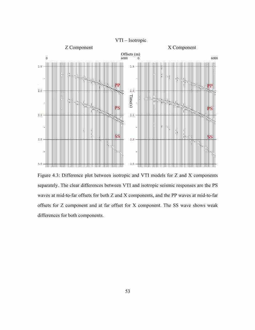
VTI – Isotropic Z Component X Component Offsets (m) 0 6000 0 6000

PP PP

Time(s)PS

SS

PS

SS

Figure 4.3: Difference plot between isotropic and VTI models for Z and X components

separately. The clear differences between VTI and isotropic seismic responses are the PS

waves at mid-to-far offsets for both Z and X components, and the PP waves at mid-to-far

offsets for Z component and at far offset for X component. The SS wave shows weak

differences for both components.

53

54

Once we set the anisotropy parameters, we can calculate the elastic constants according

to equations (2.3), (2.8) and (2.11). We can also obtain the velocities from different

propagation directions. The modeling result (Figure 4.2) shows the Z and X components

for both isotropic and VTI seismic responses. PP, PS and SS waves are included in each

component. PP wave travels the fastest, then the PS, and finally the SS wave. All these

reflections show as a single reflection, because of the tuning effect among layers. By

direct visual comparison, it is difficult to see much difference between isotropic and VTI

seismic responses at each component.

One way to examine the difference is to calculate the actual difference between two

models corresponding to the same component. Figure 4.3 shows the differences. For the

Z component, the areas of greatest difference are the PP and PS waves at mid-to-far

offsets; for the X component, the areas of greatest difference are the PP wave at far offset

and the PS wave at mid-to-far offsets. The SS wave difference appears to be weaker than

PP and PS waves for both the vertical and radial components.

There are some differences observed in Figure 4.3 that might be expected to be seen

in surface seismic data if the anisotropy is strong. In practice, the actual anisotropy may

be weaker than used for this model. Thus, I ask, is the weak anisotropy seismic response

differentiable to the isotropic response? Which portions of recorded seismic data show

greater sensitivity?

Figure 4.4 illustrates the reflection coefficient sensitivity to Thomsen’s parameters for

VTI model. Those plots are extracted from the amplitudes of the modeling figures, such

as Figure 4.2, the isotropic model, and the VTI model with γ=0.1, δ=0.1 and ε=0.1.

Figure 4.4a is the ε sensitivity test. Because ε>0 (see chapter 2), I increase ε from 0 to 0.1

at an increment of 0.05, while keeping γ and δ at constant value of 0.1. This will test

which component of each wave may be more sensitive when changing ε. The sensitivity

0 2000 40000

1

2

3

offset(m)

refle

ction

coef

ficient

Z component-PP wave

0 2000 40000

0.5

1

1.5Z component-PS wave

offset(m)

refle

ction

coef

ficient

0 2000 4000-1.5

-1

-0.5

0X component-PP wave

offset(m)

refle

ction

coef

ficient

0 2000 40000

0.5

1

1.5

offset(m)

X component-PS wave

refle

ction

coef

ficient

isotropicε=0ε=0.05ε=0.1

Figure 4.4a

0 2000 40000

1

2

3

offset(m)

refle

ctio

n co

effic

ient

Z component-PP wave

0 2000 40000

0.5

1

1.5Z component-PS wave

offset(m)

refle

ctio

n co

effic

ient

0 2000 4000-1.5

-1

-0.5

0X component-PP wave

offset(m)

refle

ctio

n co

effic

ient

0 2000 40000

0.5

1

1.5X component-PS wave

offset(m)

refle

ctio

n co

effic

ient

isotropicδ=-0.1δ=-0.05δ=0δ=0.05δ=0.1

Figure 4.4b

Figure 4.4: Reflection coefficient sensitivity test for the indicated wave and component of

the VTI model. Figure 4.4a is the ε sensitivity test for γ=0.1, δ=0.1; Figure 4.4b is the δ

sensitivity test for γ=0.1, ε=0.1. The isotropic case is for ε=0, γ=0 and δ=0. The

sensitivity parts are marked by the circles.

55

56

can be observed through the separation among the curves. The higher separation between

the curves, the more sensitive the wave component might be. Figure 4.4a shows the Z

component of the PS wave at far offset is most sensitive. Even the small change of ε

parameter may cause relatively large differences. Figure 4.4b shows the δ sensitivity test.

Because δ can be negative (see chapter 2), I vary δ from -0.1 to 0.1 at an increasing

interval of 0.05 but keeping ε=0.1 and γ=0.1. The most sensitive parts may be the areas in

the black circles: the Z component of PP wave at far offset and the X component of PS

wave at middle offset.

The sensitivity test for γ is not performed here, because this is only one shot and a

single line orientation, thus no transverse component is generated. As a result, there is no

basis for a sensitivity analysis for γ. Further, there is no test on the sensitivity of SS wave

seismic response because the SS wave reflection coefficient is very weak in the

difference (Figure 4.3).

Another way to look at the sensitivity is to plot the difference in the seismic

amplitude between isotropic and VTI anisotropy. Figure 4.5 is the sensitivity test for the

differences between isotropic and VTI models. Like Figure 4.4, ε and δ are tested in the

same way. The black circles are the areas of highest sensitivities. Note that the most

sensitive areas of the anisotropy parameters are the same as that shown in Figure 4.4, but

the separation of curves in the difference plot is more direct and clear than that in Figure

4.4.

Through this test, I show that the sensitive part of ε might be the Z component of the

PS wave at far offset, and the sensitive part of δ might be the Z component of the PP

wave at far offset and the X component of the PS wave at middle offset. These could be a

guide to analyze the data in the field.

2) Isotropic and HTI models

0 2000 4000-0.5

0

0.5

offset(m)

refle

ctio

n co

effic

ient

Z component-PP wave difference0.5

0

-0.5

57

0 2000 4000-0.5

0

0.5Z component-PS wave difference

offset(m)

refle

ctio

n co

effic

ient

0 2000 4000

X component-PP wave difference

offset(m)

refle

ctio

n co

effic

ient

0 2000 4000-0.5

0

0.5

offset(m)

X component-PS wave difference

refle

ctio

n co

effic

ient

ε=0ε=0.05ε=0.1

Figure 4.5a

0 2000 4000-0.5

0

0.5

offset(m)

refle

ctio

n co

effic

ient

Z component-PP wave difference

0 2000 4000-0.5

0


offset(m)

refle

ctio

n co

effic

ient

0 2000 4000-0.5

0

0.5X component-PP wave difference

offset(m)

refle

ctio

n co

effic

ient

0 2000 4000-0.5

0

0.5X component-PS wave differnce

offset(m)

refle

ctio

n co

effic

ient

δ=-0.1δ=-0.05δ=0δ=0.05δ=0.1

Figure 4.5b

Figure 4.5: Sensitivity test for VTI case. The plots are differences in reflection coefficient

between isotropic and VTI models. Figure 4.5a is the sensitivity test for ε at γ=0.1, δ=0.1;

Figure 4.5b is the δ sensitivity test at γ=0.1, ε=0.1. Sensitive areas are marked by circles.

58

The HTI model is based on the Hudson’s (1980, 1981) theory and is applied in Bakulin et

al.’s (2000, part I) method, on the assumption of isolated penny-shaped dry cracks

(equation 2.21). The crack density is set to be 0.08, which nearly reaches the validation

limit of 0.1 in Hudson’s model. The crack density of 0.08 for this model is relatively

large and represents strong anisotropy. With this value, using equations (2.21) and (2.13),

the elastic constants can be evaluated to provide inputs for the synthetic seismogram.

In contrast to the isotropic and VTI models, the HTI model provides azimuthal

anisotropy for horizontal seismic propagation. This means, at different line orientations,

the seismic response will be different, due to the presence of vertical fractures. Figures

4.6 to Figure 4.10 show the HTI difference plots at different line orientation. θ=0̊ means

the shot receiver line is orthogonal to fracture sets, and θ=90̊ indicates the shot receiver

line is parallel to fracture sets. By gradually changing the azimuth (Figure 4.6 to Figure

4.10), the difference in reflection coefficient changes too. The largest difference occurs at

azimuth 0 degrees, orthogonal to the fractures and the least difference shows at azimuth

90 degrees, parallel to the fractures. At azimuth 90 degrees, the difference between HTI

and isotropic seismograms is almost 0. In this case, HTI behaves as nearly isotropic

media.

At crack density of 8%, an azimuthal anisotropy change can be found (Figure 4.6 to

Figure 4.10). Figure 4.11 describes the difference plot of AVO response between

isotropic and HTI models (Bakulin’s model) at azimuth 0 degrees. Crack density varies

from 2% to 8%. The isotropic case is described as a crack density of zero. The crack

density increases 2% at each interval. It is not difficult to find out that the X component

of the PS wave at middle offset is the most sensitive. The separation of curves at middle

offset is the most obvious. The sensitivity test at other azimuths is not performed, because

the largest difference in the seismic response is at the direction orthogonal to the

HTI – Isotropic (θ=0̊)

Z Component X component

Offsets (m) 0 6000 0 6000

PPPP

Time(s)PS

SS

PS

SS

Figure 4.6: HTI difference plot at 0 degree azimuth. The shot-receiver line is orthogonal

to the fractures. We observe large difference between the HTI and isotropic seismic

responses.

59



Offsets (m) 0 6000 0 6000

Figure 4.7: HTI difference plot at 30 degree azimuth. The shot-receiver line is oriented at

30 degrees to the fractures. A large difference can be observed, yet the seismic amplitude

is a little weaker compared to Figure 4.6.

PPPP

Time(s)PS

SS

PS

SS

60



Offsets (m) 0 6000 0 6000


45 degrees to the fractures. A moderate difference can be observed. The amplitude is a

little weaker compared to Figure 4.7.

PPPP

Time(s)PS

SS

PS

SS

61



Offsets (m) 0 6000 0 6000


60 degrees to the fractures. A small difference can be observed. The seismic amplitude is

weak.

PPPP

Time(s)PS

SS

PS

SS

62



Offsets (m) 0 6000 0 6000

Figure 4.10: HTI difference plot at 90 degree azimuth. The shot-receiver line is parallel to

the fractures. There is least difference and the seismic amplitude is almost zero.

PPPP

Time(s)PS

SS

PS

SS

63

0 2000 4000-0.5

0

0.5

offset(m)

refle

ctio

n co

effic

ient

Z component-PP wave difference

0 2000 4000-0.5

0


offset(m)

refle

ctio

n co

effic

ient

0 2000 4000-0.5

0

0.5X component-PP wave difference

offset(m)

refle

ctio

n co

effic

ient

0 2000 4000-0.5

0

0.5X component-PS wave difference

offset(m)

refle

ctio

n co

effic

ient

e=0.02e=0.04e=0.06e=0.08

Figure 4.11: Crack density sensitivity test for isolated penny-shaped dry cracks. The plots

are the differences in reflection coefficient between isotropic and HTI models for the

indicated wave types and components. The black circle is the most sensitive area. For the

isotropic model, crack density e=0.

64

65

fractures. The seismic amplitude at other azimuths is weaker and is not appropriate for

the sensitivity study. The HTI model using dry cracks only may be not realistic in natural

settings, especially for a reservoir which contains irreducible water saturation, and

residual oil saturation at the same time. But this model can approximate the case of high

gas saturation.

3) HTI and orthorhombic models with one shot and areal grid of receivers

The modeled acquisition geometry of one shot and an areal grid of receivers requires

a different approach to deal with the components of the reflected waves. In the case of

one shot and one receiver line orientation, which contains the vertical and radial

components, is the same as what is recorded in the acquisition geometry, such as the Z

and X components. The natural geometry of one shot and an areal grid of receivers,

however, is not the same as recorded in acquisition geometry. The X component is

usually parallel to the receiver line, and the Y component is orthogonal to the receiver

line. When the angle between the shot and receiver is not zero, the radial and transverse

components have projections towards both X and Y components. The wavefield

separation must be done to separate the radial and transverse components from the X and

Y components (see appendix C).

After wavefield separation, we assume that the X and Y components are converted to

pure radial and transverse components. The vertical (Z) component is not affected by

this, because the horizontal wavefield separation only deals with shear wave splitting.

Figure 4.12 delineates the vertical component of the HTI model. The HTI model uses

Bakulin’s model with a crack density of 8%. The shot is at (0, 0), and X, Y are the

receiver line orientations. The X direction is orthogonal to the vertical fractures, and the

Y direction is parallel to the vertical fractures. Figure 4.12 illustrates the cube form of a

shot gather in this geometry, unlike the one shot-receiver line orientation. Z is the time

HTI Vertical Component

PP PS

SS

PP PS

SS

(s)

(m) (m)

Figure 4.12: Vertical component of HTI seismic model (Bakulin, 2000) for one shot and

areal grid of receivers geometry. The X direction is orthogonal to the vertical fractures,

and the Y direction is parallel to the vertical fractures. In the ZX plane, the amplitude is

stronger, while in ZY plane, the amplitude is weaker, showing the possible azimuthal

change.

66

67

axis. PP, PS and SS waves can be seen in ZY and ZX planes. In the ZX plane, the

amplitude is stronger, whereas in the ZY plane, the amplitude is weaker, showing the

possible azimuthal change.

A time slice along the XY plane, provides a snap shot of each wave traveling at that

time. Figure 4.13 shows the time snap shot differences between the isotropic and HTI

models before wavefield separation, and Figure 4.14 shows time snap shot difference of

isotropic and HTI models after wavefield separation. After wavefield separation, the

transverse component of the PP wave of is gone. The PP wave should not exist in the

transverse component. Further, the X component of the PS reflection in Figure 4.13 does

not show the azimuthal change as appears in Figures 4.6 to 4.10, where the maximum

difference lies at the direction orthogonal to the fractures. By contrast, the largest

difference lies somewhere near azimuth 45 degrees. After the wavefield separation as

seen in Figure 4.14, the azimuthal change of the radial component of the PS reflection

coefficient is similiar to the phenomenon of Figures 4.6 to 4.10. As it can be seen, the

largest difference lies in the X direction (normal to the fracture orientation) and the

smallest difference lies in the Y direction (parallel to the fracture orientation). For the

transverse component, the biggest difference lies approximately along azimuth 45

degrees, where the amplitude is the strongest.

The orthorhombic model is derived from the VTI and HTI combination. A VTI

background with previously used Thomsen’s parameters (0.1, 0.1, 0.1), together with the

HTI model of isolated penny-shaped, dry cracks only and a crack density of 8%

(Bakulin’s model), are used to get anisotropy parameters via equations (2.31) to (2.33).

Figure 4.15 is the time slice difference of orthorhombic and isotropic seismic models

after wavefield separation. The amplitude with azimuthal change is not obvious for the

vertical and radial components. It is also hard to locate one azimuth that has the largest

Difference: HTI-Isotropic

Vertical Component

X Component

Y Component

Figure 4.13: The time slices of HTI and isotropic seismic difference for each component

of PP, PS and SS waves before wavefield separation.

68

Difference: HTI-Isotropic

Vertical Component

Radial Component

Transverse Component

Figure 4.14: The time slices of HTI and isotropic seismic difference for each component

of PP, PS and SS waves after wavefield separation.

69

Difference: Orthorhombic-Isotropic

Vertical Component

Radial Component

Transverse Component

Figure 4.15: The time slices of orthorhombic and isotropic seismic difference for each

component of PP, PS and SS waves after wavefield separation.

70

71

amplitude difference between isotropic and orthorhombic seismograms. It is probably

due to the combination of VTI and HTI in this model, which weakens the effect of

azimuthal anisotropy. Regarding the transverse component, PP wave is gone as usual,

and PS and SS waves have a polarization reversal at a certain azimuth. In contrast to HTI,

the azimuthal anisotropy is weak as seen in the simulated seismic data.

SUMMARY

In this chapter, VTI, HTI and orthorhombic anisotropic models are introduced, and

their seismic responses are compared with the isotropic seismic response. All these

models are built on the basis of the theories of chapter 2. The difference plots and the

sensitivity study provide a guide to explore the possibility of anomalies in the seismic

data.

For the geometry of one shot-receiver line orientation, the difference of VTI and

isotropy is seismically observable in the synthetic data. The sensitivity test of Thomsen’s

parameters also reveals that the sensitive area of ε might be the Z component of the PS

wave at far offset, and the sensitive part of δ might be the Z component of the PP wave at

far offset and the X component of the PS wave at middle offset. For HTI anisotropy, the

change of seismic amplitude with azimuth is verified. The sensitivity of crack density is

found to be in the X component of the PS wave at middle offset. All these tests indicate

that multi-component data might be useful in finding the anomalies that may exist in the

seismic data.

For the geometry of one shot and an areal grid of receivers, the azimuthal change in

HTI media is still obvious compared to the above geometry. However, orthorhombic

seismic responses do not show a consistent azimuthal change of amplitude.

72

Chapter 5: Sensitivity to the middle Woodford using an HTI model


1) Test the sensitivity of seismic response to different matrix background parameters

using Vp/Vs (Vp changes) as a criteria.

2) Test the sensitivity to the thickness effect by different Vp/Vs scenarios as the

matrix background.

3) Test the sensitivity of seismic reflection at the top boundary of the middle layer to

HTI variations of matrix background Vp/Vs (Vp changes), fluid saturation and

aspect ratio.

TEST ON THE MIDDLE WOODFORD

In this chapter, I test the sensitivity of seismic reflections on the middle Woodford.

The Woodford as there exists a strong possiblity for this interval to exhibit HTI

anisotropy (See chapter 3). The upper and lower members are also important, but because

they are thin layers, the sensitivity test on those members may not be obvious to

investigate. Besides, the well log does not provide enough information to support the

possible anisotropy in the upper and lower layers.

EFFECT OF MATRIX BACKGROUND Vp/Vs

Vp/Vs can be useful as a good lithology indicator. Using well log data and seismic

data together, Vp/Vs may reveal variations in identifying lithology and fluid type (gas or

fluid) in the pore space (Tatham, 1982; Tatham and Krug, 1985). Tatham (1982) and

Castagna and Backus (1993) classified the Vp/Vs to several typical lithology type:

sandstone, shale, dolomite and limestone. Their average Vp/Vs values from laboratory

73

measurement are approximately 1.7 for water saturated sandstones, 2.0 for consolidated

shale, 1.8 for dolostone and 1.9 for limestone (Mavko et al., 2003). So the value of Vp/Vs

may be linked to the information of rock matrix type (lithology). Meanwhile, the fluid

saturated in the pore space also has a strong effect on the observed Vp/Vs value. Low

density fluids such as oil and gas may reduce the Vp/Vs, and gas saturation will greatly

reduce the Vp/Vs value to as low as 1.5. In all, Vp/Vs is influenced by the original

composition of different lithology in the rock matrix, fluid type and saturation in the pore,

pressure, stress, temprature, porosity, compaction and cementation. The way to simplify

the sensitivity test is to vary Vp/Vs under constant conditions, such as the same porosity,

pressure and temperature. The only parts we vary are the lithology and fluid type.

In Table 3.2, the Vp/Vs range in three intervals of Woodford range is from 1.54 to

1.58, and the low value of Vp/Vs may indicate gas saturation, consistent with the high

resistivity log response. The Woodford in RTC #1 is dominated by chert, with a mixture

of clay and carbonate. Thus, the Vp/Vs of Woodford may range from 1.54 to 2,

depending on the variations in lithology, fluid type, and saturation. Here, I examine

Vp/Vs in the middle layer, because the middle Woodford is the thickest unit and may be

anisotropic (HTI) as a result of vertical fractures. I only consider three cases in the middle

part: (1) Vp/Vs equals 1.54, the observed Vp/Vs value in the Woodford; (2) Vp/Vs equals

1.7, a typical value for clean liquid saturated sandstone; (3)Vp/Vs equals 2, a typical

value for well consolidated shale. Because Vs is almost unaffected by fluid type, I keep

Vs constant while varying Vp to get the matrix information. The seismic modeling still

uses the vertical impulsive source and to simplify the model description, the geometry of

an inline shot and receivers is used.

To better understand the matrix background effect on the seismic response, only an

isotropic model is considered. The physical parameters like Vp, Vs and density for the

74

upper and lower layers are kept at their original values, with the only change of Vp/Vs

in the middle layer. Specifically, only Vp varies. The models are conducted in two ways:

First with a large thickness (three layers are all 150m). Second, utilize the actual log

thicknesses 30ft, 175ft and 20ft in upper, middle and lower layers respectively. The

purpose of the first (thick) model is to see the seismic response clearly with enough

vertical resolution, and then to observe the tuning effect when the thickness changes to

smaller (observed) intervals.

Figures 5.1 and 5.2 show the Z (vertical) and X (radial) components of the seismic

responses to Vp/Vs values of 1.54, 1.7 and 2 for the thick models (150m at each interval).

The arrows indicate the location of changing PP wave. The first arrow (horizontal)

indicates the top of middle Woodford reflection, and the second arrow (slanted) is an

indicator of bottom middle Woodfood reflection. In Figure 5.1, the PP wave reflection of

the top of the middle layer has strong positive amplitude in the Z component at Vp/Vs of

1.54, while decreasing to nearly zero at Vp/Vs of 1.7. At Vp/Vs of 2.0, the polarity is

reversed, showing strong negative amplitude.

The bottom reflection, however, has an increasing positive amplitude from low

Vp/Vs to high Vp/Vs. The 150m layer thickness enables us to see clearly the change in

seismic amplitude under these circumstances. The Vp in the middle layer is gradually

increasing to reach the Vp value of upper layer, and finally to exceed it. That is why the

polarity reversal occurs at Vp/Vs of 2.0. PS and SS waves do not change, due to the lack

of change in Vs. For the X component of Figure 5.2, similar phenomenon is observed.

The PP wave reflection on the top of the middle Woodford first shows a negative

amplitude at Vp/Vs of 1.54, then weakens to zero at Vp/Vs of 1.7, and changes to a

positive amplitude at Vp/Vs of 2.0. The base of the middle layer reflection has an

increasing negative amplitude as the Vp/Vs rises (Vp rises).

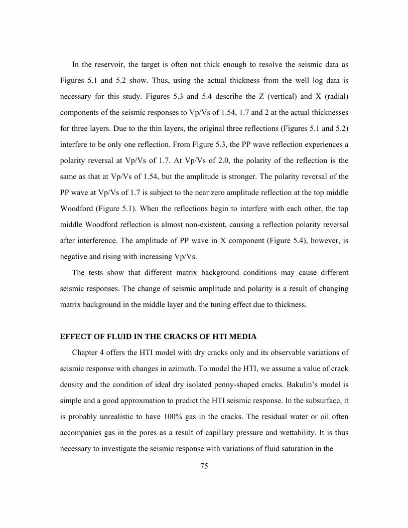
75

In the reservoir, the target is often not thick enough to resolve the seismic data as

Figures 5.1 and 5.2 show. Thus, using the actual thickness from the well log data is

necessary for this study. Figures 5.3 and 5.4 describe the Z (vertical) and X (radial)

components of the seismic responses to Vp/Vs of 1.54, 1.7 and 2 at the actual thicknesses

for three layers. Due to the thin layers, the original three reflections (Figures 5.1 and 5.2)

interfere to be only one reflection. From Figure 5.3, the PP wave reflection experiences a

polarity reversal at Vp/Vs of 1.7. At Vp/Vs of 2.0, the polarity of the reflection is the

same as that at Vp/Vs of 1.54, but the amplitude is stronger. The polarity reversal of the

PP wave at Vp/Vs of 1.7 is subject to the near zero amplitude reflection at the top middle

Woodford (Figure 5.1). When the reflections begin to interfere with each other, the top

middle Woodford reflection is almost non-existent, causing a reflection polarity reversal

after interference. The amplitude of PP wave in X component (Figure 5.4), however, is

negative and rising with increasing Vp/Vs.

The tests show that different matrix background conditions may cause different

seismic responses. The change of seismic amplitude and polarity is a result of changing

matrix background in the middle layer and the tuning effect due to thickness.

EFFECT OF FLUID IN THE CRACKS OF HTI MEDIA

Chapter 4 offers the HTI model with dry cracks only and its observable variations of

seismic response with changes in azimuth. To model the HTI, we assume a value of crack

density and the condition of ideal dry isolated penny-shaped cracks. Bakulin’s model is

simple and a good approxmation to predict the HTI seismic response. In the subsurface, it

is probably unrealistic to have 100% gas in the cracks. The residual water or oil often

accompanies gas in the pores as a result of capillary pressure and wettability. It is thus

necessary to investigate the seismic response with variations of fluid saturation in the

Z Component (150m)

Vp/Vs=1.54 Vp/Vs=1.7 Vp/Vs=2.0

Offsets(m) Offsets(m) Offsets(m) 0 6000 0 6000 0 6000

PP PP PP

Time(s)

PS

SS

PS

SS

PS

SS

PS

SS

Figure 5.1: Z (vertical) component of seismic responses to Vp/Vs of 1.54, 1.7 and 2 at

thick layers (150m). The arrows suggest the change of PP wave.

76

X Component (150m)



PPPP PP

Time(s) PS

SS

PS

SS

PS

SS

Figure 5.2: X (radial) component of seismic responses to Vp/Vs of 1.54, 1.7 and 2 at

thick layers (150m). The arrows suggest the change of PP wave.

77

Z Component (actual thickness)



PPPP PP

Time(s)

PS

SS

PS

SS

PS

SS

Figure 5.3: Z (vertical) component of seismic responses to Vp/Vs of 1.54, 1.7 and 2 at

actual layer thickness.

78

X Component (actual thickness)



PPPP PP

Time(s) PS

SS

PS

SS

PS

SS

Figure 5.4: X (radial) component of seismic responses to Vp/Vs of 1.54, 1.7 and 2 at

actual layer thickness.

79

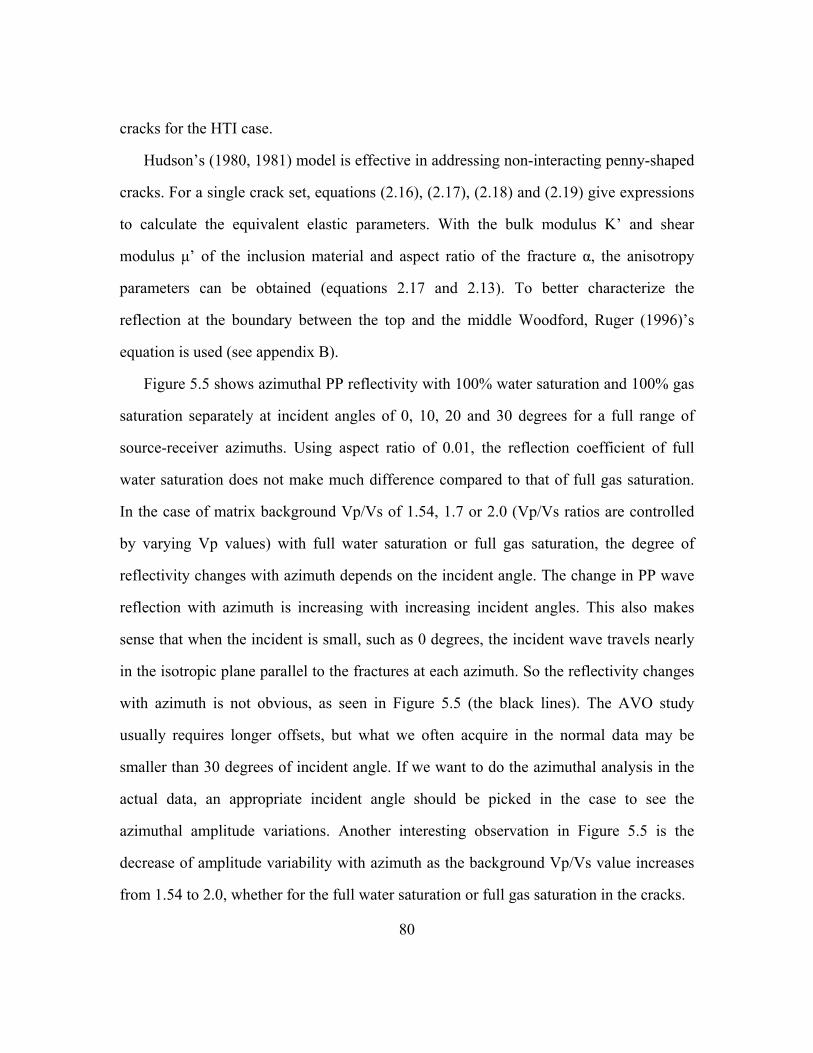
80

cracks for the HTI case.

Hudson’s (1980, 1981) model is effective in addressing non-interacting penny-shaped

cracks. For a single crack set, equations (2.16), (2.17), (2.18) and (2.19) give expressions

to calculate the equivalent elastic parameters. With the bulk modulus K’ and shear

modulus μ’ of the inclusion material and aspect ratio of the fracture α, the anisotropy

parameters can be obtained (equations 2.17 and 2.13). To better characterize the

reflection at the boundary between the top and the middle Woodford, Ruger (1996)’s

equation is used (see appendix B).

Figure 5.5 shows azimuthal PP reflectivity with 100% water saturation and 100% gas

saturation separately at incident angles of 0, 10, 20 and 30 degrees for a full range of

source-receiver azimuths. Using aspect ratio of 0.01, the reflection coefficient of full

water saturation does not make much difference compared to that of full gas saturation.

In the case of matrix background Vp/Vs of 1.54, 1.7 or 2.0 (Vp/Vs ratios are controlled

by varying Vp values) with full water saturation or full gas saturation, the degree of

reflectivity changes with azimuth depends on the incident angle. The change in PP wave

reflection with azimuth is increasing with increasing incident angles. This also makes

sense that when the incident is small, such as 0 degrees, the incident wave travels nearly

in the isotropic plane parallel to the fractures at each azimuth. So the reflectivity changes

with azimuth is not obvious, as seen in Figure 5.5 (the black lines). The AVO study

usually requires longer offsets, but what we often acquire in the normal data may be

smaller than 30 degrees of incident angle. If we want to do the azimuthal analysis in the

actual data, an appropriate incident angle should be picked in the case to see the

azimuthal amplitude variations. Another interesting observation in Figure 5.5 is the

decrease of amplitude variability with azimuth as the background Vp/Vs value increases

from 1.54 to 2.0, whether for the full water saturation or full gas saturation in the cracks.


0 200-0.06

-0.04

-0.02

0

Azimuth(degrees)

PP R

efle

ctiv

ity

100% water saturation

0 200-0.06

-0.05

-0.04

-0.03

-0.02100% gas saturation

Azimuth(degrees)

PP R

efle

ctiv

ity

0 200-0.02

0

0.02

0.04100% water saturation

Azimuth(degrees)

PP

Ref

lect

ivity

0 200-0.01

0

0.01

0.02

0.03100% gas saturation

Azimuth(degrees)

PP

Refle

ctiv

ity

0 2000.05

0.1

0.15100% water saturation

Azimuth(degrees)

PP

Ref

lect

ivity

0 2000.06

0.08

0.1

0.12100% gas saturation

Azimuth(degrees)

PP R

efle

ctiv

ity

Figure 5.5: PP reflection coefficient changes with azimuth 0-360 degrees at different

incident angles for matrix background Vp/Vs of 1.54, 1.7 and 2.0. The aspect ratio is

0.01. Each line color indicates a different incident angle.

81

For Vp/Vs of 2.0 at full gas saturation, there is an azimuthal polarity reversal (the trough

turns to be peak or the peak turns to be the trough at the same location) at 30 degrees (red

line), which behaves very differently in contrast to the case of full water saturation.

Knowing the behaviors for full water saturation or gas saturation is not enough. New

ways to calculate the fluids in the cracks should be implemented. This leads to the issue

of fluid substitution in shale at low effective porosity (pores in shale are isolated mostly),

an area of active research. In this study, to estimate the effective elastic modulus of a

fluid mixture, we use the Voigt average and Reuss average (Mavko et al., 2003) :

82

i1

N

v ii

M f M=

= ∑ (5.1)

1

1 Ni

iR i

fM M=

=∑ (5.2)

where if is the volume fraction of the ith element of the effective media, iM is the

elastic modulus of ith element, vM is the Voigt effective average elastic modulus, RM

is the Reuss effective average elastic modulus and N is the number of phases. The Voigt

average is also called isostrain average and Reuss average is also called isostress average.

To determine the elastic constants of the fluid mixture in the cracks, patchy saturation

(approximated by Voigt average) and uniform saturation (approximated by Reuss

average) can be used (Sava, 2005).

Figure 5.6 shows the computed PP reflectivity changes with azimuth and Vp versus

gas saturation using patchy and uniform saturation (Voigt and Reuss average) for

different fluid saturation. The matrix background Vp/Vs is 1.54 and incident angle is 20

degrees. A combination of water and gas is considered in the cracks, oil is not taken into

consideration here. In Figure 5.6, arrows point toward decreasing water saturation and

increasing gas saturation. The color bar on the bottom is an expression of change of gas

saturation. The azimuthal reflectivity is quite different for patchy and uniform saturation

83

for different water and gas saturation. For patch saturation, the curves of fluid saturation

push upward, but for uniform saturation, vice versa. Both Vp values decrease with

increasing gas saturation, but the decreasing trend is different. This suggests that the

different methods to calculate the fluid stiffnesses in the cracks may cause different

seismic responses. In this study, the patchy saturation is used, considering the mixture of

gas and water may not uniformly distribute in the cracks.

Figure 5.7 illustrates PP reflectivity with azimuthal change for three matrix

background Vp/Vs ratios at combination of water and gas saturation using Voigt average

(patchy saturation). The incident angle is 20 degrees and the aspect ratio is 0.01. The

arrows point toward increasing gas saturation (decreasing water saturation). Within

Figure 5.7, with increasing Vp/Vs, there is a tendency for the PP reflectivity to change

the azimuthal polarity at larger gas saturation. For Vp/Vs of 1.7, azimuthal polarity

changes at a gas saturation of 100%; and for Vp/Vs of 2.0, azimuthal polarity changes at

a gas saturation of 90%. The seismic amplitude here, is more sensitive to larger Vp/Vs

ratio at higher gas saturation. The matrix background and the fluid saturation may be the

sensitive parameters deciding the change of seismic response.

EFFECT OF ASPECT RATIO

We know how matrix background and fluid saturation in the crack influence the

seismic response, and how long the offsets (incident angle) have impact on the azimuthal

seismic analysis, yet the aspect ratio of crack is set to be constant. We still do not know

the effect of aspect ratio, one important property of the cracks. Aspect ratio describes the

openness of the crack. From Figures 5.8 to 5.10, the aspect ratio has been tested,

including Vp/Vs in each figure. The incident angles are all 20 degrees and the arrow

points out the direction of increasing gas saturation.

0 100 200 300

-0.05

-0.045

-0.04

Azimuth(degrees)

PP R

efle

ctiv

ityVoigt Average

0 50 1001.356

1.358

1.36

1.362

1.364x 104

Gas Saturation(%)

Vp(ft

/s)

0 100 200 300

-0.05

-0.045

-0.04

Azimuth(degrees)

PP R

efle

ctiv

ity

Reuss Average

0 50 1001.356

1.358

1.36

1.362

1.364x 104

Gas Saturation(%)

Vp(ft

/s)

Figure 5.6: PP reflectivity changes with azimuth, together with Vp versus gas saturation

using Voigt and Reuss average separately. The matrix background Vp/Vs is 1.54, the

incident angle is 20 degrees and the aspect ratio is 0.01. Gas saturation (Sg) is from 0 to

100% (see the horizontal color bar). Arrows point toward increasing gas saturation.

84

0 100 200 300

-0.05

-0.045

-0.04

Azimuth(degrees)P

P R

efle

ctiv

ity

Matrix background Vp/Vs=1.54

0 100 200 3000

0.005

0.01

0.015

Azimuth(degrees)

PP R

efle

ctiv

ity


0 100 200 3000.09

0.1

0.11

Azimuth(degrees)

PP R

efle

ctiv

ity


Figure 5.7: PP reflectivity with azimuthal changes for three Vp/Vs ratios at incident angle

of 20 degrees and at combination of water and gas saturation (Sg) using Voigt average.

The aspect ratio is set to be 0.01. Arrows point toward increasing gas saturation.

85

86

≥

With decreasing aspect ratio, the azimuthal curves are pushing upward. For matrix

background Vp/Vs of 1.54 in Figure 5.8, whatever the aspect ratio varies, there is no

azimuthal polarity change at any water and gas saturation. For Vp/Vs of 1.7 in Figure 5.9,

azimuthal polarity starts to get reversed at aspect ratio larger than 0.005. When aspect

ratio equals 0.1, the first azimuthal polarity change occurs at Sg (gas saturation) of 70%.

For Vp/Vs of 2.0 in Figure 5.10, azimuthal polarity changes at aspect ratio larger than

0.001. All the curves with different saturation get reversed. To better understand the

effect of aspect ratio, I extracted the curves of all aspect ratios at Sg (gas saturation) of

70%, which may be typical for the Woodford Shale with higher gas saturation. Figure

5.11 shows the results of extraction. At higher Vp/Vs and higher aspect ratio, the polarity

of azimuthal reflectivity tends to change. The tendency of changing azimuthal polarity

also occurs at larger gas saturation (Figure 5.9, Sg 70%). In particular, when Vp/Vs is

larger, azimuthal polarity reversal can be seen at a relative smaller aspect ratio (Figure

5.10, at aspect ratio of 0.005 shows a phenomenon of azimuthal polarity reversal).

SUMMARY

This chapter considers the comprehensive factors (matrix background, fluid type)

which may affect the seismic reflection response. Matrix background Vp/Vs value, fluid

saturation, aspect ratio in the cracks, offsets (incident angles) show the combined effects

on the seismic amplitude. Assuming matrix background Vp/Vs only relies on Vp and

according to the half space assumption, the azimuthal polarity tends to be reversed at

larger Vp/Vs, larger aspect ratio and higher gas saturation. Understanding how these

physical factors interactive with each other to influence the seismic response may be

helpful in the interpretation of the field data in future.


0 100 200 300

-0.05

-0.045

-0.04

Azimuth(degrees)

PP R

efle

ctiv

ity

Aspect ratio=0.1

0 100 200 300

-0.05

-0.045

-0.04

Azimuth(degrees)

PP R

efle

ctiv

ity

Aspect ratio=0.05

0 100 200 300

-0.05

-0.045

-0.04

Azimuth(degrees)

PP R

efle

ctiv

ity

Aspect ratio=0.01

0 100 200 300

-0.05

-0.045

-0.04

Azimuth(degrees)

PP

Refle

ctiv

ity

Aspect ratio=0.005

0 100 200 300

-0.05

-0.045

-0.04

Azimuth(degrees)

PP

Refle

ctiv

ity

Aspect ratio=0.001

Figure 5.8: PP azimuthal reflectivity for matrix background Vp/Vs of 1.54 at aspect ratios

of 0.1, 0.05, 0.01, 0.005 and 0.001. Arrow points toward increasing gas saturation (Sg).

87


0 100 200 300

-2

0

2

4

6

8

10x 10-3

Azimuth(degrees)

PP R

efle

ctiv

ity

Aspect ratio=0.1

0 100 200 300

0

5

10x 10-3

Azimuth(degrees)

PP R

efle

ctiv

ity

Aspect ratio=0.05

0 100 200 300

0

5

10

15x 10-3

Azimuth(degrees)

PP R

efle

ctiv

ity

Aspect ratio=0.01

0 100 200 300

0

5

10

15x 10-3

Azimuth(degrees)

PP

Refle

ctiv

ity

Aspect ratio=0.001

0 100 200 300

0

5

10

15x 10-3

Azimuth(degrees)

PP

Refle

ctiv

ity

Aspect ratio=0.005



88


0 100 200 300

0.09

0.095

0.1

0.105

Azimuth(degrees)

PP R

efle

ctiv

ity

Aspect ratio=0.1

0 100 200 300

0.09

0.095

0.1

0.105

Azimuth(degrees)

PP R

efle

ctiv

ity

Aspect ratio=0.05

0 100 200 300

0.09

0.095

0.1

0.105

0.11

Azimuth(degrees)

PP R

efle

ctiv

ity

Aspect ratio=0.01

0 100 200 300

0.09

0.095

0.1

0.105

0.11

Azimuth(degrees)

PP

Refle

ctiv

ity

Aspect ratio=0.005

0 100 200 3000.095

0.1

0.105

0.11

Azimuth(degrees)

PP

Refle

ctiv

ity

Aspect ratio=0.001



89

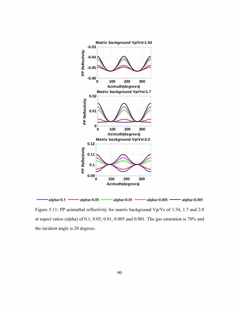
0 100 200 300-0.06

-0.05

-0.04

-0.03

Azimuth(degrees)PP

Ref

lect

ivity


0 100 200 3000

0.01

0.02

Azimuth(degrees)

PP R

efle

ctiv

ity


0 100 200 3000.09

0.1

0.11

0.12

Azimuth(degrees)

PP R

efle

ctiv

ity


Figure 5.11: PP azimuthal reflectivity for matrix background Vp/Vs of 1.54, 1.7 and 2.0

at aspect ratios (alpha) of 0.1, 0.05, 0.01, 0.005 and 0.001. The gas saturation is 70% and

the incident angle is 20 degrees.

90

91

Chapter 6: Discussions and Conclusions

I have applied anisotropic seismic modeling for different models (VTI, HTI and

orthorhombic models) to the middle Woodford Shale, in order to test the seismic

sensitivities to different anisotropic scenarios. These models were based on the analysis

of the RTC #1 well log data. Density, gamma ray, resistivity, sonic, dipole sonic logs,

part of imaging (FMI) logs, elemental capture spectroscopy (ECS) and X-ray diffraction

(XRD) data from the core samples were studied to decide possible isotropic model and

anisotropic parameters. Real layer thicknesses from well logs were used as the dimension

of input models. Elastic properties such as density, P-wave velocity and S-wave velocity

were averaged for seismic modeling.

I conducted these models using a vertical impulsive source and three component

receivers. The vertical impulsive source generated P-P, P-SV and SV-SV waves. To

make the synthetic model easier, I mainly used an acquisition geometry of one shot and

one receiver line orientation (one shot and areal grid of receivers were also used to check

the HTI and orthorhombic seismic responses for the transverse component).

I showed that there was an apparent difference between isotropic and anisotropic

seismic responses. Strong anisotropy parameters had large effects on the synthetic

seismic data in terms of amplitude variation. I demonstrated that HTI model showed a

clear azimuthal amplitude with different shot-receiver line orientation towards the

fracture. VTI anisotropy did not have amplitude variation with the azimuth, because the

horizontal layer was almost isotropic for all the azimuths.

I conducted a sensitivity study by changing different physical paramters, which

caused seismic amplitude variations and azimuthal variations. I found that large

sensitivities occurred in the mid-offset range for P-SV wave (especially for radial

92

component) and in the far-offset range for P-P and P-SV waves (espically for vertical

component). I also showed how synthetic seismic response was senstive to Vp/Vs, fluid

saturation and aspect ratio. The azimuthal polarity changed (peak changed to be trough or

trough changed to be peak) tended to occur at relatively larger aspect ratio, larger gas

saturation and larger Vp/Vs. These findings helped understand how these parameters

influence the seismic response, so that these properties can be addressed when dealing

with field data.

This work was mainly based on the well logs and borehole data of one single well,

which did not have sufficient information to determine if there was notable anisotropy

and to determine the appropriate anisotropic model we should use. Due to the limited

information, I conducted the model by assuming one type of anisotropy (VTI, HTI or

orthorhombic anisotropy) in the middle layer at each time. Other assumptions included

averaged physical properties within each Woodford layer and ideal penny-shaped crack

for the HTI model. In reality, the fractures may not be penny-shaped and anisotropy may

not be observed from seismic data because of the resolution, the quality of seismic data

and processing artifacts. In spite of the shortcomings, the sensitivity results from the

synthetic seismic response suggested multi-component data were useful for the

anisotropic analysis. The sensitive offset range for different component and different

types of waves was a guide in determining the location for analyzing the anisotropy of

prestack seismic data. Future work will include investigating complex fracture models,

include more available well logs, and combine well log data with multicomponent

seismic data.

Appendix A

APPROXIMATIONS FOR ISOTROPIC AVO

The Zoeppritz equations are very useful in describing the seismic reflection. However,

they are very complex and do not have any descriptions of the physical meanings of the

elastic parameter and density. Many recent researchers, such as Aki and Richards (1980),

Shuey (1985), Hilterman (1989) and Thomsen (1990), have given different forms of

approximations to Zoeppritz equations. These approximations are based on the

assumption of small reflectivity of the boundary between upper and lower layers, and

mostly only applicable to small offsets (<30 ). Beyond this limit, the approximations are

not valid any more. Castagna and Backus (1993) provided a good overview of these

approximations for conventional AVO analysis.

°

1) Aki and Richards (1980)

In a similar fashion, Aki and Richards (1980) demonstrated that the approximation to a

simple interface has a reflectivity for plane wave as:

93

22 2( ) sin sin cosRpp A B Cθ θ θ= + + θ , (A.1)

where

2

1 ( )21 2( ) (2 )212

VpAVpVp Vs VsB

Vp Vp VsVpC

Vp

ρρ

ρρ

Δ Δ= +

Δ Δ Δ= − +

Δ=

.

(A.2)

Here , ,Vp Vs ρ are the average values across the boundary for the P wave velocity, shear

wave velocity and density. ,VpΔ VsΔ and ρΔ are the difference values across the

boundary for the P wave velocity, shear wave velocity and density. θ is the incident angle

and ( )Rpp θ is PP wave reflectivity.

2) Shuey (1985)

Shuey (1985) remained the same expressions for A and C in equation (A.2), but

derived an alternative expression for B:

2

3 7 1 2 1( ) ( )2 2 1 (1 )

VpBVp

σ σ ρ σσ σ ρ σ

− Δ − Δ= − − + Δ

− − − , (A.3)

where σ is Poisson’s ratio, which is defined by the forms of Vp/Vs: 2

2

1 ( / ) 2(2 ( / ) 1

Vp VsVp Vs

σ )−=

− , (A.4)

A is the normal incidence reflection coefficient, B predominates at intermediate angle

and C is dominant as the critical angle is approached. Since for a small angle incidence

with restricted values, an even simpler linear equation can be performed: 2( ) sinRpp A Bθ θ≈ + . (A.5)

3) Hilterman (1989)

Hilterman (1989) derived another simple approximation, assuming Vp/Vs=2.0, as

follows: 2( ) cos 2.25 sinRpp A 2θ θ σ≈ + Δ θ , (A.6)

where σΔ is the Poisson’s ratio contrast across the boundary. At small angles, A is

dominant (equation A.2), while at larger angles, σΔ is dominant. That is, at near offset,

normal reflection coefficients have large impact on the PP wave reflectivity, and at far

offset, differences of Poisson’s ratio contrast control the trend of reflection.

4) Thomsen (1990)

Thomsen (1990) indicated that the introduction to the term σ into equation (A.3) has

complicated the term. He introduced another term μ, shear modulus to replace slope B of

Shuey’s equation: 21 ( 2( )

2Vp VsB

Vp Vp)μ

μΔ Δ

= −, (A.7)

94

where μΔ is the shear modulus contrast across the boundary and μ is the average shear

modulus.

The linear approximations to the Zoeppritz equations are meaningful. It not only

reduces the complexity, but also introduces the physical parameters. The approximations

are valid through small impedance contrast and near offset angles, which exist widely in

the real seismic data acquisition. In particular for AVO analysis in prestack data, a far

offset angle larger than 30 degrees is hard to obtain during the seismic acquisition. Thus,

approximations are very useful and easy to be applied in the industry.

95

Appendix B

APPROXIMATIONS FOR ANISOTROPIC AVO

The existence of anisotropy can affect the seismic reflectivity. Since Thomsen (1986)

introduced the anisotropy parameters, some researchers, such as Ruger (1995, 1996) and

Chen (1995) derived the approximate expressions of AVO for anisotropic media. The

anisotropy AVO can be very different from isotropic AVO, because of the new

introduction to anisotropy parameters into the equations. Mavko et al. (2003) gave a good

overview of these theories.

1) PP wave reflection for weakly anisotropic VTI media

Thomsen (1993) derived the approximation form of PP wave reflection for weakly

anisotropic VTI media, according to the assumption of small impedance contrast. The

equation is shown as below: ( ) ( ) ( )iso anisoRpp Rpp Rppθ θ− −= + θ , (B.1)

where 2 2( ) sin sin cos2 2anisoRpp 2δ εθ θ θ− θΔ Δ

≈ +

( )isoRpp θ− is the same as equations (A.1) and (A.2), which are in terms of isotropic

media. δΔ and εΔ are the Thomsen’s parameters’ contrast across the boundary. The

AVO difference between isotropy and anisotropy is the anisotropic term ( )anisoRpp θ− ,

which is represented by the terms of δΔ and εΔ .

2) PP wave reflection for weakly anisotropic HTI media

Ruger (1995, 1996) and Chen (1995) gave an approximation form of PP wave

reflection between two HTI media sharing the same symmetry axis. For the P wave in the

vertical symmetry plane parallel to the horizontal axis, the reflectivity can be written as:

2 2 22( 0 , ) ( ) ( ( ) )sin sin cos

2 2isoVsRpp Rpp

Vp2δ εϕ θ θ γ θ θ− θΔ Δ

= ° = + + Δ +, (B.2)

96

where ϕ is the azimuth angle measured from horizontal axis, and θ is the incident

angle defined with respect to vertical axis.

Ruger (1996) also derived the equations of azimuthal AVO approximations for both

vertical symmetry plane and non-symmetry plane. For vertical symmetry plane

perpendicular to the symmetry axis, it is: ( 90 , ) (isoRpp Rpp )ϕ θ − θ= ° ≈ . (B.3)

For the non-symmetry plane,

2 22( , ) ( ) (( ( ) ) cos )sin2iso

VsRpp RppVp

2δϕ θ θ γ ϕ− θΔ≈ + + Δ

4 2 2 2( cos sin cos )sin cos2 2

2ε δϕ ϕ φ θ θΔ Δ+ +

. (B.4)

This equation describes the AVO response for azimuthal anisotropy.

Whatever for the VTI and HTI AVO approximations, the PP reflectivity is expressed

as the combination of isotropic and anisotropic terms. The isotropic term is the same as

described in appendix A. The anisotropic term dominants the change of reflectivity due to

anisotropy. Understanding the anisotropy parameters could help understand the variations

of the PP wave reflectivity.

97

Appendix C

HORIZONTAL COMPONENTS (RADIAL AND TRANSVERSE) WAVEFIELD

SEPARATION

Mu et al. (2007) provided a good overview on the horizontal components wavefield

separation. For the near surface, low velocity zone often exists. The reflection wave

which passes through the low velocity zone, usually travels to the surface vertically,

making the P wave recorded by vertical component and the S saves recorded by

horizontal components. This is true for the case that the source-receiver direction is

parallel to the receiver line direction. The receiver line direction is the orientation of X

component, Y component is orthogonal to X component. However, when there is an

angle that is not equal to zero between the source-receiver direction and the receiver line

direction, the horizontal components (radial and transverse) will have their projections on

both directions. Thus, it is necessary to separate the radial and transverse components

from the X and Y components recorded in the acquisition coordinate.

In Figure C.1, the source is labeled as red explosion; the receivers are labeled as black

triangle. SG is the bottom receiver line; the upper receiver line is the same as SG. For one

receiver R in the figure, SR is the source-receiver direction. Ux is X component, Uy is Y

component recorded in the field; Ur is radial component and Ut is transverse component

in the natural coordinate. If we assume θ is the angle between SR and SG, then the

relationship between X, Y components and radial, transverse components is:

98

⎞⎟⎠

. (C.1)

cos sinsin cos

Ur UxUt Uy

θ θθ θ

⎛ ⎞ ⎡ ⎤ ⎛=⎜ ⎟ ⎜⎢ ⎥−⎝ ⎠ ⎣ ⎦ ⎝

Thus, as long as we know the θ, radial and transverse components can be separated from

X and Y components.

Specially, angle θ can be obtained when the distance between receivers and between

receiver lines is available.

Figure C.1: The relationship of wavefield separation.

99

100

References

Aki, K., and P. G. Richards, 1980, Quantitative seismology, theory and methods: W. H. Freeman and Co., San Francisco, vol. I, 557 p., vol. II, 373 p.

Ali, W., 2009, Lithofacies, depositional environment, burial history and calculation of organic richness from the wireline logs: a study of Barnett Shale in the Delaware Basin, Pecos Co., West Texas, and comparison with the Barnett Shale in the Fort Worth Basin: M.S. thesis, Jackson School of Geosciences, The University of Texas at Austin, p. 11, 49, 67, 189-193.

Andrews, R. D, 2009, Production decline curves and payout threshold of horizontal Woodford wells in the Arkoma Basin, Oklahoma: Shale Shaker, 60, 103-112.

Aoudia, K., J. Miskimins, C. Mnich and N. B. Harris, 2009, Analysis of rock mechanical properties by mineralogy and their potential effect from hydraulic fracturing in the Woodford shale: 2009 AAPG Annual Convention and Exhibition, AAPG Search and Discovery Article #90090.

Backus, G. E, 1962, Long-wave elastic anisotropy produced by horizontal layering: Journal of Geophysical Research, 67, 4427-4440.

Bakulin, A., V. Grechka, and I. Tsvankin, 2000, Estimation of fracture parameters from reflection seismic data—Part I: HTI model due to a single fracture set: Geophysics, 65, 1788-1802.

Bakulin, A., V. Grechka, and I. Tsvankin, 2000, Estimation of fracture parameters from reflection seismic data—Part II: fractured models with orthorhombic symmetry: Geophysics, 65, 1803-1817.

Berge, P. A., 1995, Constraints on elastic parameters and implications for lithology in VTI media: Society of Exploration Geophysicists international Expo and 65th annual meeting, 4 p.

Berryman, J. G., 1979, Long wave elastic anisotropy in transversely isotropic media: Geophysics, 44, 896-917.

Boughal, K., 2008, Special focus: North America outlook unconventional resources: Geopete’s View, http://geopetesview.blogspot.com/2009_02_21_archive.html.

Boyd, D. T., 2009, Oklahoma 2008 drilling highlights: Shale Shaker, March-April, 10 p.

http://geopetesview.blogspot.com/2009_02_21_archive.html

101

Brown, A., 2007, Paleo Heat Flow in North American Late Paleozoic Foreland Basins: Constraints from Permian Basin of West Texas: AAPG Hedberg Research Conference, The Hague, the Netherlands, Search and Discovery Article #90066.

Brown, R., and J. Korringa, 1975, On the dependence of the elastic properties of a porous rock on the compressibility of the pore fluid: Geophysics, 40, 608-616.

Cardott, B. J., 2008, Overview of Woodford gas-shale play of Oklahoma: 2008 AAPG Annual Convention, AAPG Search and Discovery Article #90078.

Castagna, J. P., and M. M. Backus, 1993, Offset-dependent reflectivity-theory and practice of AVO analysis: Society of Exploration Geophysics, p. 7-10, 20, 40, 135-167.

Chen, W., 1995, AVO in azimuthally anisotropic media: fracture detection using P wave data and a seismic study of naturally fractured tight gas reservoirs: Ph.D. dissertation, Stanford University, 143 p.

Cheng, C. H., 1978, Seismic velocities in porous rocks: direct and inverse problems: Ph.D. thesis, MIT, Cambridge, Massachusetts, 255 p.

Cheng, C. H., 1993, Crack models for a transversely anisotropic medium: J. Geophys. Res., 98, 675-684.

Comer, J. B., 1991, Potential for producing oil and gas from Woodford Shale (Devonian-Mississippian) in the Southern Mid-continent, USA: 1991 AAPG annual convention meeting, AAPG Search and Discovery Article #91004.

Comer, J. B., 1991, Stratigraphic analysis of the upper Devonian Woodford Formation, Permian Basin, West Texas and Southeastern New Mexico: Bureau of Economics Geology, The University of Texas at Austin, Report of investigations No. 201, 63 p.

Comer, J. B., 2007, Reservoir characteristics and production potential of the Woodford Shale in the southern midcontinent: PowerPoint Presentation, https://scholarworks.iu.edu/dspace/handle/2022/1826.

Comer, J. B., 2008, Reservoir characteristics and production potential of the Woodford Shale: World Oil, 229, 83-89.

Curtis, J. B., 2002, Fractured shale-gas systems: AAPG Bulletin, 86, 1921-1938.

Daley, P. F., and F. Hron, 1979, Reflection and transmission coefficient in transversely isotropic media: Geophysics, 44, 27-38.

https://scholarworks.iu.edu/dspace/handle/2022/1826

102

Dutton, S. P., E. M. Kim, R. F. Broadhead, W. D. Raatz, C. L. Breton, S. C. Ruppel, and C. Kerans, 2005, Play analysis and leading-edge oil-reservoir development methods in the Permian basin: increased recovery through advanced technologies: AAPG Bulletin, 89, 553-576.

Ellison, S. P., 1950, Subsurface Woodford black shale, West Texas and Southeast New Mexico: Bureau of Economic Geology, University of Texas at Austin Report Investigations 7, 20 p.

Eshelby, J. D., 1957, The determination of the elastic field of an ellipsoidal inclusion, and related problems: Proc. Royal Soc. London, Series A, Mathematical and Physical Sciences, 241, 376-396.

Frantz, J. H., and V. Jochen, 2005, When your gas reservoir is unconventional, so is our solution: http://www.pe.tamu.edu/wattenbarger/public_html/Selected_papers/--Shale%20Gas/shale_gas-%20schlumberger.pdf.

Gutschick, R., and C. Sandberg, 1983, Mississippian continental margins on the conterminous United States, in D. J. Stanley and Moore. G. T., The shelf break: Critical interface on continental margins: SEPM Special Publication 33, p. 79–96.

Helbig, K., 1979, Discussion on the “reflection, refraction and diffraction of waves in media with elliptical velocity dependence” by F. K. Levin: Geophysics, 44, 987-990.

Hester, T.C., H.L. Sahl, and J.W. Schmoker, 1988, Cross sections based on gamma-ray, density, and resistivity logs showing stratigraphic units of the Woodford Shale, Anadarko Basin, Oklahoma: U.S. Geological Survey Miscellaneous Field Studies Map MF-2054, 2 sheets.

Hester, T.C., J.W. Schmoker, and H.L. Sahl, 1990, Log-derived regional source-rock characteristics of the Woodford Shale, Anadarko Basin, Oklahoma: U.S. Geological Survey Bulletin 1866-D, 38 p.

Hilterman, F. J., 1989, Is AVO the seismic signature of rock properties? : 59th Ann. Internat. Mtg: Soc. of Expl. Geophys., Expanded Abstracts, 559.

Hudson, J. A., 1980, Overall properties of a cracked solid: Math. Proc. Camb. Phil. Soc., 88, 371.

Hudson, J. A., 1981, Wave speeds and attenuation of elastic waves in material containing cracks: Geophys. J. R. astr. Soc., 64, 133-150.

Hudson, J. A., 1986, A higher order approximation to the wave propagation constants for a cracked solid: Geophys. J. R. astr. Soc., 87, 265-274.

http://www.pe.tamu.edu/wattenbarger/public_html/Selected_papers/--Shale%20Gas/shale_gas-%20schlumberger.pdf

http://www.pe.tamu.edu/wattenbarger/public_html/Selected_papers/--Shale%20Gas/shale_gas-%20schlumberger.pdf

103

Jones, R. W., 1981, Some mass balance and geological constraints on migration mechanisms: AAPG Bulletin, 65, 103–122.

King, P. B., 1942, Permian of West Texas and southeastern New Mexico: AAPG, 26, 535-763.

Lambert, M. W., 1982, Vitrinite reflectance of Woodford in Anadarko basin, Oklahoma: AAPG, 66, 591-592.

Li, Y., 2002, Anisotropy well logs and their applications in seismic analysis: 2002 SEG annual meeting, Expanded Abstracts, 21, 2459-2462.

Mavko, G., T. Mukerji and J. Dvorkin., 2003, The Rock physics handbook: tools for seismic analysis in porous media: Cambridge University Press, p. 19-26, 67-69, 110-112, 133-142, 292-299.

Mu, Y., and X. Chen, Y. Liu, G. Li and S. Wang, 2007, Seismic data processing method: Petroleum Industry Press, p. 204-205.

Ostrander, W. J., 1983, Method for interpretation of seismic records to yield indication of gaseous hydrocarbons: Acoustical Society of America Digital Library, 73, 714-714.

Ostrander, W. J., 1984, Plane wave reflection coefficients for gas sands at nonnormal angles of incidence: Geophysics, 49, 1937-1648.

Portas, R. M., and R. Slatt, 2010, Characterization and origin of fracture patterns in a Woodford shale quarry in Southeastern Oklahoma for application to exploration and development: 2010 AAPG annual convention and exhibition, AAPG search and discover article #90104.

Ruger, A., 1995, P wave reflection coefficients for transversely isotropic media with vertical and horizontal axis of symmetry: Society of Exploration Geophysics, 65th annual international meeting, Expanded abstracts, p. 278-281.

Ruger, A., 1996, Variation of P wave reflectivity with offset and azimuth in anisotropic media: Society of Exploration Geophysics, 66th annual international meeting, Expanded abstracts, p. 1810-1813.

Ruger, A., 2002, Reflection coefficients and azimuthal AVO analysis in anisotropic media: Society of Exploration Geophysics, Tulsa, Oklahoma, p. 39-99.

Ruppel, S. C., and R. G. Loucks, 2008, The devonian Woodford Fm of the Permian Basin: Complex depositional and temporal variations across from anaerobic marine basin: 2008 AAPG Annual Convention and Exhibition Abstracts Volume, 17, 175.

104

Rutherford, S. R., and R. H. Williams, 1989, Amplitude-versus-offset variations in gas sands: Geophysics, 54, 680-688.

Sava, D., 2005, Quantitative data integration for fracture characterization using statistical rock physics: Ph.D. dissertation, Stanford University, Department of Geophysics, p. 9-10, 118-124.

Schoenberg, M., 1980, Elastic wave behavior across linear slip interfaces, J. Acoust. Soc. Am., 68, 1516-1521.

Schoenberg, M., 1983, Reflection of elastic waves from periodically stratified media with interfacial slip: Geophysical Prospecting, 31, 265-292.

Schoenberg, M., and J. Douma, 1988, Elastic wave propagation in media with parallel fractures and aligned cracks: Geophysical Prospecting, 36, 571-590.

Schoenberg, M., and F. Muir, 1989, A calculus for finely layered anisotropic media: Geophysics, 54, 581–589.

Shuey, R. T., 1985, A simplification of the Zoeppritz equations: Geophysics, 50, 609-614.

Tatham, R. H., 1982, Vp/Vs and lithology: Geophysics, 47, 336-344.

Tatham, R. H. and E. H. Krug, 1985, Vp/Vs interpretation: Developments in Geophysical Exploration Methods-6, Ch. 5, p. 139-188.

Tatham, R. H. and M. D. McCormack, 1991, Multicomponent in petroleum exploration: Society of Exploration Geophysics, 243 p.

Thomsen, L., 1986, Weak elastic anisotropy: Geophysics, 51, 1954-1966.

Thomsen, L., 1990, Poisson was not a geophysicist: Geophysics, the Leading Edge of Exploration, 9, 27-29.

Thomsen, L., 1993, Weak anisotropic reflections: in Offset Dependent Reflectivity- Theory and Practice of AVO analysis, Castagna and Backus, Invest. Geophysics, NO. 8, Society of Exploration Geophysicists, Tulsa, Oklahoma, p. 103-111.

Thomsen, L., 1995, Elastic anisotropy due to aligned cracks in porous rock: Geophysical Prospecting, 43, 805-829.

Tsvankin, I., 1997, Anisotropic parameters and P wave velocity for orthorhombic media: Geophysics, 62, 1292-1309.

105

Tsvankin, I., 1997, Reflection moveout and parameter estimation for horizontal transverse isotropy: Geophysics, 62, 614-629.

Vernik, L., and X. Liu, 1997, Velocity anisotropy in shales: a petrophysical study: Geophysics, 62, 521-532.

Walsh, J. J, B. K. Sinha, and M. Ammerman, 2008, Derivation of anisotropy parameters in a shale using borehole sonic data: 2008 American Rock Mechanics Association, 08-272.

Wang, H. and R. P. Philp, 1997, Geochemical study of potential source rocks in the Anadarko Basin, Oklahoma: AAPG Bulletin, 81, 249-275.

Zoeppritz, K., 1919, Erdbebenwellen VIIB, On the reflection and propagation of seismic waves: Gottinger Nachrichten, I, p. 66-84.

106

Vita

Na Shan was born in Changchun, Jilin, China, the only child of her family. After

graduating from Changchun Experimental Middle School, she entered China University

of Petroleum, Beijing and was awarded with Bachelor of Science Degree in 2007. Since

she was in the petroleum school, she became interested in the exploration geophysics and

decided to receive further education after she graduated. She joined the M.S. program in

Jackson School of Geosciences, the University of Texas at Austin for exploration

geophysics in 2008 and interned with ION GXT in 2010. She has one abstract published

in the SEG 2010 annual meeting.

Email address: [email protected]

This thesis was typed by Na Shan.

copyright by na shan 2010

Documents