Copyright

by

Jason Zhi Liang

2015

The Thesis Committee for Jason Zhi LiangCertifies that this is the approved version of the following thesis:

Evolutionary Bilevel Optimization for Complex Control

Problems and Blackbox Function Optimization

APPROVED BY

SUPERVISING COMMITTEE:

Risto Miikkulainen, Supervisor

Peter Stone

Evolutionary Bilevel Optimization for Complex Control

Problems and Blackbox Function Optimization

by

Jason Zhi Liang, B.S.EECS

THESIS

Presented to the Faculty of the Graduate School of

The University of Texas at Austin

in Partial Fulfillment

of the Requirements

for the Degree of

MASTER OF SCIENCE IN COMPUTER SCIENCE

THE UNIVERSITY OF TEXAS AT AUSTIN

May 2015

This thesis is dedicated to all the UTCS Masters students that are looking

forward to graduation.

Acknowledgments

I wish to thank Risto Miikkulainen for his invaluable advice and feed-

back that helped guide my research. I will also like to acknowledge everyone

in the Neural Network Research Group (NNRG), especially Julian Bishop, for

their helpful contributions and suggestions during my research talk. Lastly, I

like to thank Peter Stone for agreeing to help review my thesis.

v

Evolutionary Bilevel Optimization for Complex Control

Problems and Blackbox Function Optimization

Jason Zhi Liang, M.S.Comp.Sci.

The University of Texas at Austin, 2015

Supervisor: Risto Miikkulainen

Most optimization algorithms must undergo time consuming param-

eter tuning in order to solve complex, real-world control tasks. Parameter

tuning is inherently a bilevel optimization problem: The lower level objective

function is the performance of the control parameters discovered by an opti-

mization algorithm and the upper level objective function is the performance

of the algorithm given its parameterization. In the first part of this thesis, a

new bilevel optimization method called MetaEvolutionary Algorithm (MEA) is

developed to discover optimal parameters for neuroevolution to solve control

problems. In two challenging benchmarks, double pole balancing and heli-

copter hovering, MEA discovers parameters that result in better performance

than hand tuning and other automatic methods. In the second part, MEA

tunes an adaptive genetic algorithm (AGA) that uses the state of the popula-

tion every generation to adjust parameters on the fly. Promising experimental

results are shown for standard blackbox benchmark functions. Thus, bilevel

vi

optimization in general and MEA in particular are promising approaches for

solving difficult optimization tasks.

vii

Table of Contents

Acknowledgments v

Abstract vi

List of Tables x

List of Figures xi

Chapter 1. Introduction 1

1.1 Problem Domain . . . . . . . . . . . . . . . . . . . . . . . . . 1

1.2 Neuroevolution . . . . . . . . . . . . . . . . . . . . . . . . . . 2

1.3 Bilevel Optimization . . . . . . . . . . . . . . . . . . . . . . . 4

1.4 Overview and Organization of Thesis . . . . . . . . . . . . . . 6

Chapter 2. Related Work 8

Chapter 3. Algorithm Description 11

3.1 MEA: A metaevolutionary algorithm for bilevel optimization . 11

3.2 Evolving an Adaptive Genetic Algorithm with MEA . . . . . . 14

Chapter 4. Experimental Results 17

4.1 Experiment Setup . . . . . . . . . . . . . . . . . . . . . . . . . 17

4.2 MEA in Double Pole Balancing . . . . . . . . . . . . . . . . . 18

4.3 MEA in Helicopter Hovering . . . . . . . . . . . . . . . . . . . 23

4.4 MEA in Evolving an Adaptive Genetic Algorithm . . . . . . . 26

Chapter 5. Discussion and Future Work 31

5.1 Analysis of Experimental Results . . . . . . . . . . . . . . . . 31

5.2 Future Work . . . . . . . . . . . . . . . . . . . . . . . . . . . . 33

viii

Chapter 6. Conclusion 35

Chapter 7. Appendix 36

7.1 Details of Control Tasks . . . . . . . . . . . . . . . . . . . . . 36

7.2 Parameters, Constraints, and Default values . . . . . . . . . . 37

7.3 Evolved Parameters . . . . . . . . . . . . . . . . . . . . . . . . 38

Bibliography 41

Vita 46

ix

List of Tables

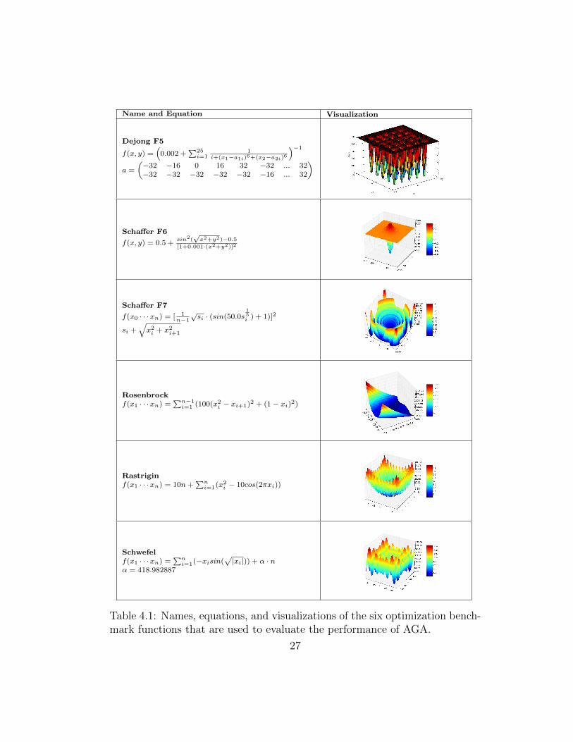
4.1 Names, equations, and visualizations of the six optimizationbenchmark functions that are used to evaluate the performanceof AGA. . . . . . . . . . . . . . . . . . . . . . . . . . . . . . . 27

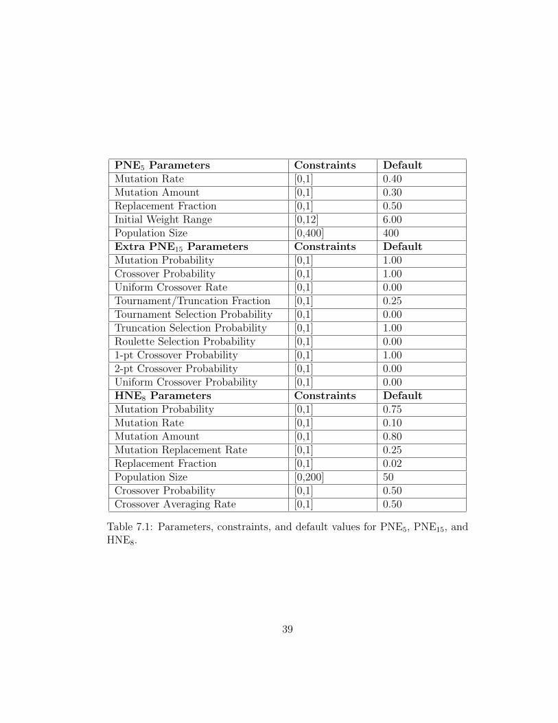
7.1 Parameters, constraints, and default values for PNE5, PNE15,and HNE8. . . . . . . . . . . . . . . . . . . . . . . . . . . . . . 39

7.2 Evolved parameters for PNE5, PNE15, and HNE8 by MEA. . . 40

x

List of Figures

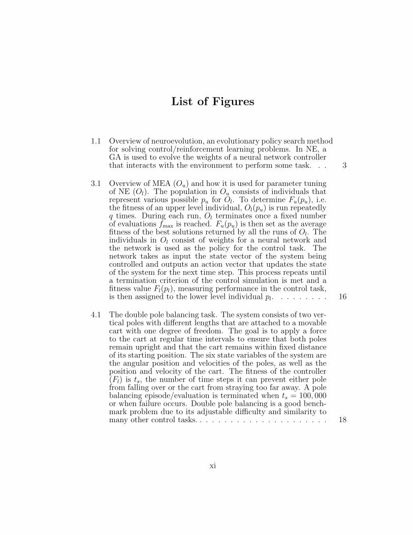
1.1 Overview of neuroevolution, an evolutionary policy search methodfor solving control/reinforcement learning problems. In NE, aGA is used to evolve the weights of a neural network controllerthat interacts with the environment to perform some task. . . 3

3.1 Overview of MEA (Ou) and how it is used for parameter tuningof NE (Ol). The population in Ou consists of individuals thatrepresent various possible pu for Ol. To determine Fu(pu), i.e.the fitness of an upper level individual, Ol(pu) is run repeatedlyq times. During each run, Ol terminates once a fixed numberof evaluations fmax is reached. Fu(pu) is then set as the averagefitness of the best solutions returned by all the runs of Ol. Theindividuals in Ol consist of weights for a neural network andthe network is used as the policy for the control task. Thenetwork takes as input the state vector of the system beingcontrolled and outputs an action vector that updates the stateof the system for the next time step. This process repeats untila termination criterion of the control simulation is met and afitness value Fl(pl), measuring performance in the control task,is then assigned to the lower level individual pl. . . . . . . . . 16

4.1 The double pole balancing task. The system consists of two ver-tical poles with different lengths that are attached to a movablecart with one degree of freedom. The goal is to apply a forceto the cart at regular time intervals to ensure that both polesremain upright and that the cart remains within fixed distanceof its starting position. The six state variables of the system arethe angular position and velocities of the poles, as well as theposition and velocity of the cart. The fitness of the controller(Fl) is ts, the number of time steps it can prevent either polefrom falling over or the cart from straying too far away. A polebalancing episode/evaluation is terminated when ts = 100, 000or when failure occurs. Double pole balancing is a good bench-mark problem due to its adjustable difficulty and similarity tomany other control tasks. . . . . . . . . . . . . . . . . . . . . . 18

xi

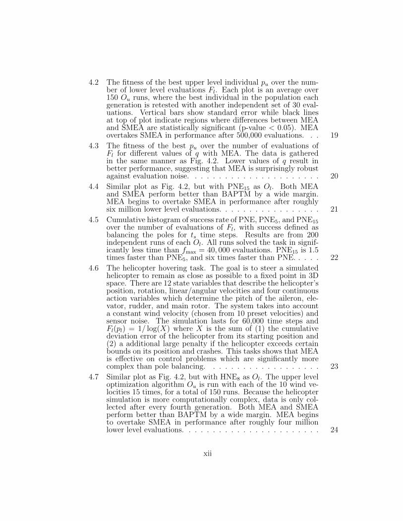
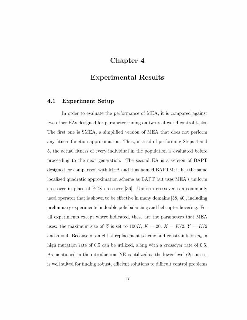
4.2 The fitness of the best upper level individual pu over the num-ber of lower level evaluations Fl. Each plot is an average over150 Ou runs, where the best individual in the population eachgeneration is retested with another independent set of 30 eval-uations. Vertical bars show standard error while black linesat top of plot indicate regions where differences between MEAand SMEA are statistically significant (p-value < 0.05). MEAovertakes SMEA in performance after 500,000 evaluations. . . 19

4.3 The fitness of the best pu over the number of evaluations ofFl for different values of q with MEA. The data is gatheredin the same manner as Fig. 4.2. Lower values of q result inbetter performance, suggesting that MEA is surprisingly robustagainst evaluation noise. . . . . . . . . . . . . . . . . . . . . . 20

4.4 Similar plot as Fig. 4.2, but with PNE15 as Ol. Both MEAand SMEA perform better than BAPTM by a wide margin.MEA begins to overtake SMEA in performance after roughlysix million lower level evaluations. . . . . . . . . . . . . . . . . 21

4.5 Cumulative histogram of success rate of PNE, PNE5, and PNE15over the number of evaluations of Fl, with success defined asbalancing the poles for ts time steps. Results are from 200independent runs of each Ol. All runs solved the task in signif-icantly less time than fmax = 40, 000 evaluations. PNE15 is 1.5times faster than PNE5, and six times faster than PNE. . . . . 22

4.6 The helicopter hovering task. The goal is to steer a simulatedhelicopter to remain as close as possible to a fixed point in 3Dspace. There are 12 state variables that describe the helicopter’sposition, rotation, linear/angular velocities and four continuousaction variables which determine the pitch of the aileron, ele-vator, rudder, and main rotor. The system takes into accounta constant wind velocity (chosen from 10 preset velocities) andsensor noise. The simulation lasts for 60,000 time steps andFl(pl) = 1/ log(X) where X is the sum of (1) the cumulativedeviation error of the helicopter from its starting position and(2) a additional large penalty if the helicopter exceeds certainbounds on its position and crashes. This tasks shows that MEAis effective on control problems which are significantly morecomplex than pole balancing. . . . . . . . . . . . . . . . . . . 23

4.7 Similar plot as Fig. 4.2, but with HNE8 as Ol. The upper leveloptimization algorithm Ou is run with each of the 10 wind ve-locities 15 times, for a total of 150 runs. Because the helicoptersimulation is more computationally complex, data is only col-lected after every fourth generation. Both MEA and SMEAperform better than BAPTM by a wide margin. MEA beginsto overtake SMEA in performance after roughly four millionlower level evaluations. . . . . . . . . . . . . . . . . . . . . . . 24

xii

4.8 The fitness of the best individual over the number of evaluationsof Fl by HNE and HNE8. Results are averaged over 500 runs,with 50 runs for each of the 10 wind velocities. HNE8 bothlearns faster and achieves higher peak fitness than HNE. . . . 25

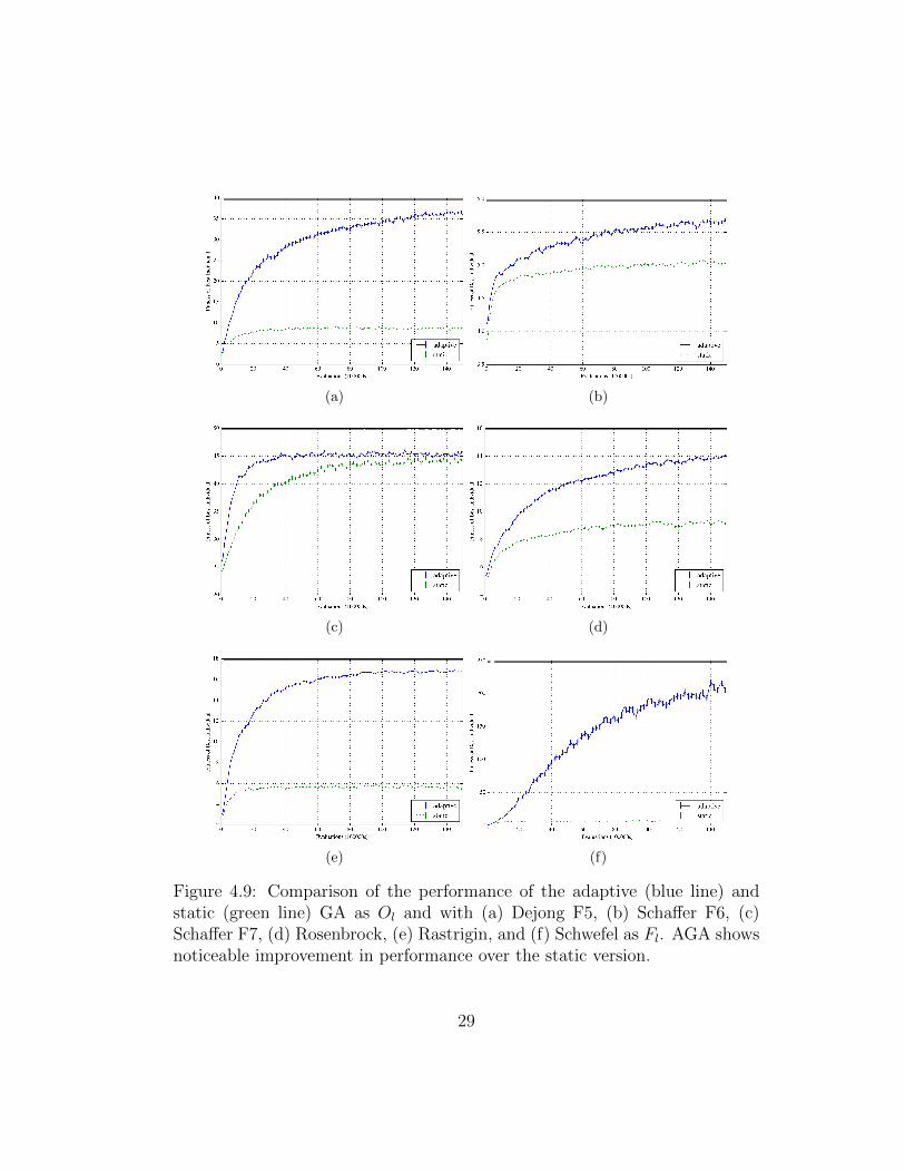
4.9 Comparison of the performance of the adaptive (blue line) andstatic (green line) GA as Ol and with (a) Dejong F5, (b) Schaf-fer F6, (c) Schaffer F7, (d) Rosenbrock, (e) Rastrigin, and (f)Schwefel as Fl. AGA shows noticeable improvement in perfor-mance over the static version. . . . . . . . . . . . . . . . . . . 29

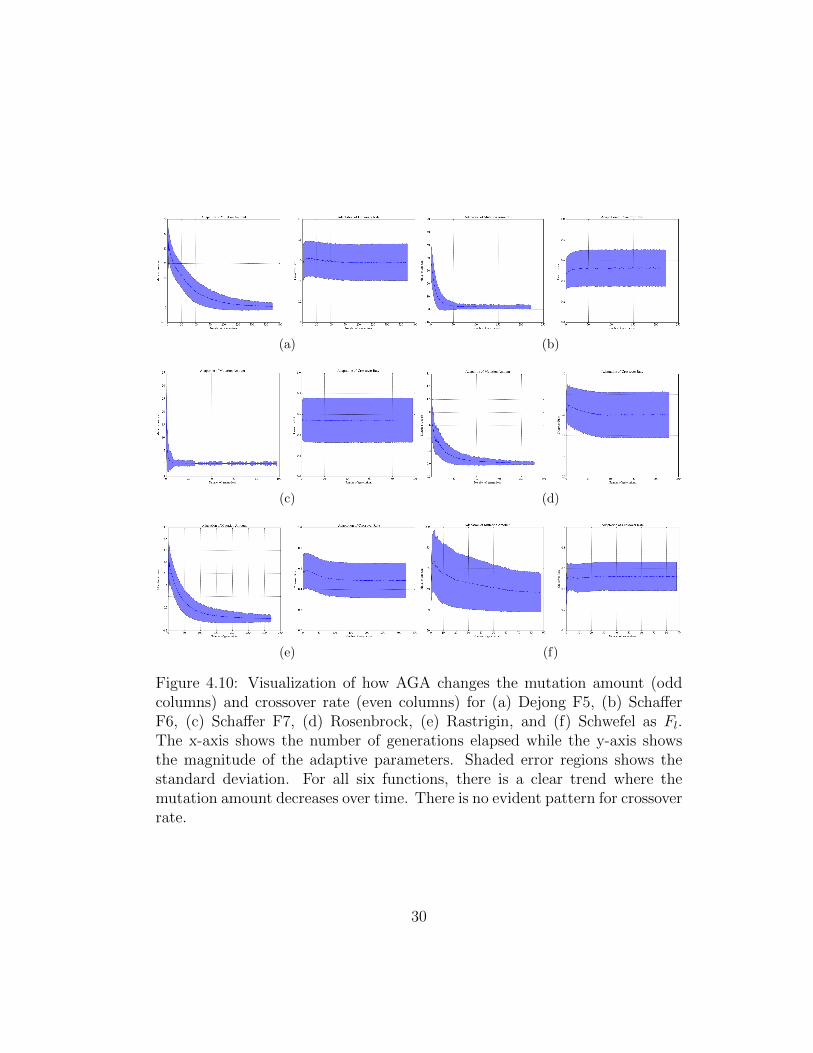
4.10 Visualization of how AGA changes the mutation amount (oddcolumns) and crossover rate (even columns) for (a) Dejong F5,(b) Schaffer F6, (c) Schaffer F7, (d) Rosenbrock, (e) Rastrigin,and (f) Schwefel as Fl. The x-axis shows the number of gen-erations elapsed while the y-axis shows the magnitude of theadaptive parameters. Shaded error regions shows the standarddeviation. For all six functions, there is a clear trend wherethe mutation amount decreases over time. There is no evidentpattern for crossover rate. . . . . . . . . . . . . . . . . . . . . 30

7.1 The topology of the neural network used in the double pole-balancing task. The inputs are position and velocity of the cart(X, X), and the angles and angular velocities of the two poles

(θ1, θ1, θ2, θ2). The output is an action moving the cart left orright. . . . . . . . . . . . . . . . . . . . . . . . . . . . . . . . . 37

7.2 The topology of the neural network used in the helicopter hov-ering task. Input variables x, y, z represent the position of thehelicopter, u, v, w represent linear velocity, and φ, θ, ω representthe angular velocity of the helicopter. The rotation of the he-licopter (roll, pitch, yaw) is not utilized. The output of thenetwork are the aileron pitch (a1), elevator pitch (a2), rudderpitch (a3), and main rotor collective pitch (a4). . . . . . . . . 38

xiii

Chapter 1

Introduction

There are many problem domains where traditional optimization al-

gorithms such as gradient descent are insufficient. Evolutionary algorithms

(EAs) are a promising approach for solving such problems but their perfor-

mance are highly dependent on having the right parameters. This chapter will

examine such problem domains, EAs, and methods for automatic parameter

tuning of EAs.

1.1 Problem Domain

For many traditional control tasks that involve few state variables, clas-

sical approaches such as PID controllers are sufficient [4]. However, many

modern control problems involve a large number of state of variables that in-

teract in a nonlinear manner, making it difficult to apply classical methods

to them [21]. A common way to solve such problems is to pose the control

task as a reinforcement learning (RL) problem where the goal is to find an

optimal policy function that maps states to actions [7]. Given the state of the

system as input, an optimal policy outputs a control action that maximizes

the performance of the system with respect to some reward criteria.

1

Traditional RL methods are based on tabular representations and dy-

namic programming; it is difficult to extend these methods to large, partially

observable continuous state spaces in many modern control problems. Re-

cently, much progress has been made in using policy search methods to solve

such control tasks [5, 6, 27]. Instead of trying to compute a Q-value for each

possible combination of state and action, the policy function is parametrized

as a fixed set of parameters p and optimization algorithms are used to find

argmaxpE(π(p)), where E(π) is the expected reward obtained by following

the policy π. For many control problems, the fitness landscape described by

E(π) is non-convex and sometimes even non-differentiable, which means gra-

dient descent is intractable and heuristic based approaches such as EAs must

be used instead [18, 23].

1.2 Neuroevolution

This thesis builds on a particular approach called neuroevolution (NE)

[17, 30, 45] that combines EAs and neural networks to search for an optimal

policy. In NE, the policy is encoded by a neural network controller where

the input is the observation vector and the output is an action vector. Neu-

ral networks can approximate arbitrary functions smoothly and are suitable

for parameterizing a control policy. As shown by Fig. 1.1, NE uses a genetic

algorithm (GA; a particular type of EA) to tune the weights of the neural

network. A blackbox optimization algorithm, the GA uses evolutionary op-

erators inspired by biological evolution to iteratively improve upon a popu-

2

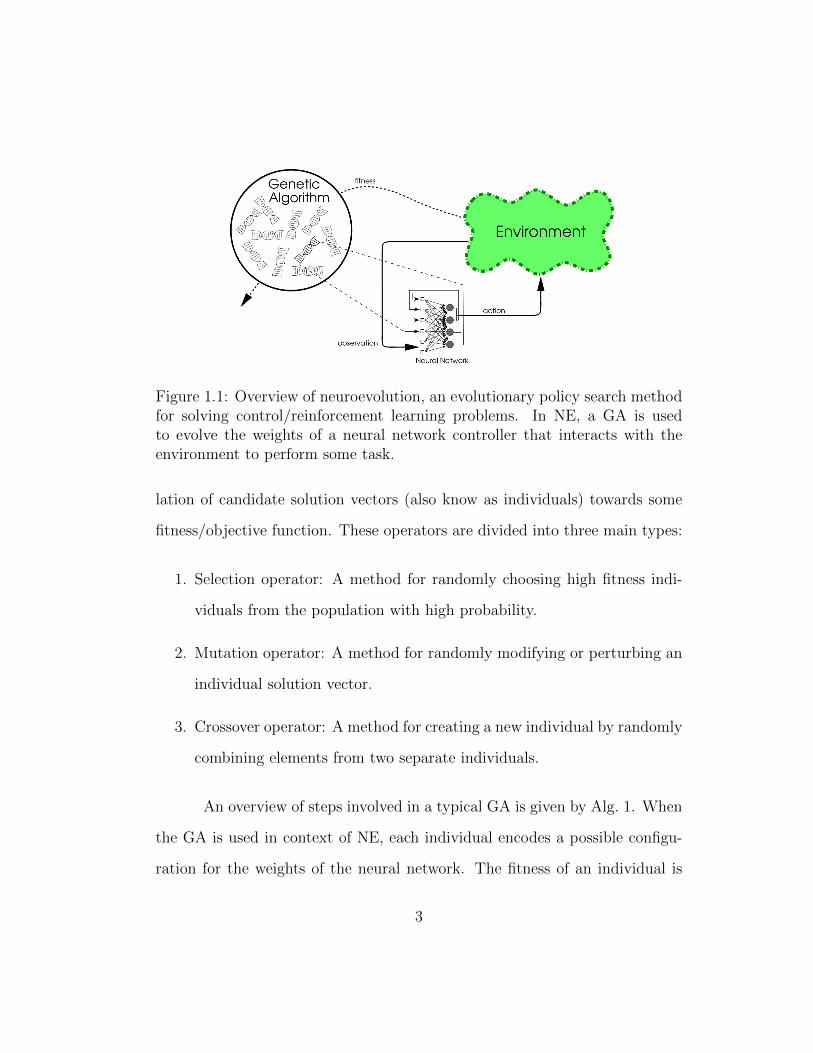
Figure 1.1: Overview of neuroevolution, an evolutionary policy search methodfor solving control/reinforcement learning problems. In NE, a GA is usedto evolve the weights of a neural network controller that interacts with theenvironment to perform some task.

lation of candidate solution vectors (also know as individuals) towards some

fitness/objective function. These operators are divided into three main types:

1. Selection operator: A method for randomly choosing high fitness indi-

viduals from the population with high probability.

2. Mutation operator: A method for randomly modifying or perturbing an

individual solution vector.

3. Crossover operator: A method for creating a new individual by randomly

combining elements from two separate individuals.

An overview of steps involved in a typical GA is given by Alg. 1. When

the GA is used in context of NE, each individual encodes a possible configu-

ration for the weights of the neural network. The fitness of an individual is

3

the performance of the associated neural network controller on some control

or reinforcement learning task. NE has been demonstrated to perform well in

many complex control problems, such as finless rocket stabilization, race-car

driving, bipedal walking, and helicopter hovering [2, 20, 28, 42].

Algorithm 1: Genetic Algorithm

1 Initialize population with K random individuals.2 Evaluate fitness of all individuals in population on some

fitness/objective function.3 Select high fitness individuals Ih from population.4 Create X new individuals In from Ih through application of

mutation and crossover.5 Replace X low fitness individuals Il with In.6 Repeat from Step 2 until a termination criterion is reached.

1.3 Bilevel Optimization

One major issue with EAs is that their performance is highly sensitive

to the parameters used. Even more so than gradient based optimization al-

gorithms, incorrectly set parameters not only make EAs run slowly but make

it difficult for them to converge onto the optimal solution. A commonly used

and yet vastly inefficient parameter tuning method is grid search [31], where

the parameter space is discretized and all possible combinations of parameters

are exhaustively evaluated. The computational complexity of grid search in-

creases exponentially with the dimensionality of the parameters. It becomes

computationally intractable once the number of parameters exceeds three or

four.

4

This problem with grid search can be avoided by framing parameter

tuning as a bilevel optimization problem [37]. Formally, a bilevel problem has

two levels: an upper level optimization task with parameters pu and objec-

tive function Fu, and a lower level optimization task with parameters pl and

objective function Fl. The goal is to find a pu that allows pl to be optimally

solved:

maximizepu

Fu(pu) = E[Fl(pl)|pu]subject to pl = Ol(pu),

(1.1)

where E[Fl(pl)|pu] is the expected performance of the lower level solution pl

obtained by lower level optimization algorithm Ol with pu as its parameters.

The maximization is done by a separate upper level optimization algorithm

Ou.

In the first part of the thesis, Ou is the proposed MEA, pu are the

parameters for NE, Ol is NE, pl are the weights of the neural network, and

Fl measures performance in two simulated and separate control tasks: double

pole balancing and helicopter hovering. As will be shown, the right heuristics

for Ou allow optimal parameters for Ol to be found much faster than with grid

search. Specifically, MEA makes use of fitness approximation to reduce the

number of Fu evaluations by Ou.

The second part of the thesis is based on an observation that GAs

often perform better on some fitness functions or optimization problems when

parameters such as mutation rate or crossover rate are allowed to vary based

5

on the current state of the population [39, 41]. Most adaptive GAs use fixed

heuristics for changing parameters, but MEA can be used to evolve an Ol

that optimally adapts certain elements of pu during the optimization of Fl. In

particular, MEA will be used to tune the weights of a neural network controller

so that it takes the state of the population as input and outputs the optimal

parameters for Ol for that generation.

1.4 Overview and Organization of Thesis

The thesis makes the following new contributions:

1. Casting parameter tuning for neuroevolution as a bilevel optimization

problem.

2. Presenting an efficient upper level algorithm Ou that achieves best results

to date on two real-world control tasks.

3. Showing that a more complex parameterization of Ol can increase its

potential performance.

4. Showing that an adaptive Ol can exceed the performance of static Ol on

a set of blackbox benchmark problems.

The rest of the thesis is organized as follows: Related work on param-

eter tuning and adaptive GAs is first summarized. The MEA algorithm and

its use in evolving an adaptive Ol are described in detail. MEA is evaluated

6

in the double pole balancing and helicopter hovering tasks, comparing its per-

formance to other hand-designed and automatic parameter tuning methods.

An adaptive and static Ol (both tuned by MEA) are compared using standard

benchmark functions for evaluating the performance of blackbox optimization

algorithms.

7

Chapter 2

Related Work

Automatic parameter tuning is a widely studied problem. A survey and

systematic categorization of current existing techniques is provided by Eiben

and Smit [15]. Many conventional methods for parameter tuning are funda-

mentally based on the grid search approach (evaluating all possible parameter

configurations) with additional heuristics to reduce computational complexity

by a constant factor [1, 31]. Examples include racing algorithms that try to

prune out bad parameters aggressively [9]. However, such approaches quickly

become intractable as the number of parameters increases beyond three or

four.

Modern algorithms for parameter tuning focus on searching through the

space of parameter configurations intelligently. One such example is ParamILS

[25], which combines hill climbing with restart heuristics. Recently, metaevo-

lutionary algorithms have been developed for the parameter tuning problem

as well [3, 13, 22, 32]. In metaevolution, the upper level algorithm Ou is an EA

and the objective function of Ou is the performance of Ol, another EA that

solves the target problem. Although more efficient than brute-force search,

metaevolution is inherently a nested procedure and still computationally com-

8

plex. To address this issue, in a method called GGA [3], the upper level

population is divided into two genders and only a subset of the population

every generation is evaluated. Furthermore, because EA’s are stochastic, it

is only possible to estimate the performance of Ol by averaging results from

multiple runs. Diosan and Oltean [13] attempted to alleviate this problem by

not optimizing pu but instead optimizing the order in which genetic operators

such as mutation and crossover are applied to the population.

Metaevolutionary algorithms are closely related to but distinct from

self-adaptive EAs [29]. The main difference is that metaevolution attempts to

find optimal parameters in an offline environment whereas self-adaptive EAs

do so online. Self-adaptive EAs thus can change their parameters dynamically

based on the state of the population [29]. On the other hand, they run slower

than EAs with static, tuned parameters.

There are a variety of diverse approaches for creating an adaptive GA.

In one approach [39], the authors propose setting a unique mutation and

crossover rate for each individual based on its fitness in relation with the

fitnesses of the rest of the population. Another paper [14] describes how an

adaptive GA can be learned by framing it as a classic reinforcement learning

problem. Q-learning is then used to discover a policy that maps the state of

the population to the optimal values for parameters such as population size,

mutation and crossover rate.

Most current research into metaevolutionary algorithms focuses on fit-

ness function approximation to reduce computational complexity [32, 37]. The

9

fitness function of the upper level, Fu(pu), is not always determined by running

Ol(pu), but is sometimes estimated using a regression model. Numerous mod-

els have been proposed, including both parametric and nonparametric ones

[24, 26, 33, 34]. BAPT, the most recent such algorithm [37], uses a local-

ized quadratic approximation model and achieves good results on classic test

problems. However, BAPT has not been tested on real-world problems and

in problems with more than three parameters in pu. Such more challenging

problems are the focus of this thesis.

10

Chapter 3

Algorithm Description

This chapter examines some of the limitations encountered with an

existing metaevolutionary algorithm such as BAPT and how MEA is able to

overcome these limitations. An adaptive GA that can be evolved with MEA

is also described.

3.1 MEA: A metaevolutionary algorithm for bilevel op-timization

MetaEvolutionary Algorithm (MEA) is fundamentally a real valued ge-

netic algorithm [11]. It is a type of EA that uses genetic operators such as

selection, mutation, crossover, and replacement to improve the overall fitness

of a population of solutions, represented by vectors of real numbers, itera-

tively over generations. MEA serves as the upper level algorithm Ou while a

GA that evolves an encoding of the weights of a neural network (NE) serves

as the lower level algorithm Ol. The roles of both MEA and NE within the

bilevel optimization framework are described in detail by Fig. 3.1. A step by

step summary of MEA is given by Alg. 2.

In BAPT [37], Fu(pu) is sometimes approximated using a regression

11

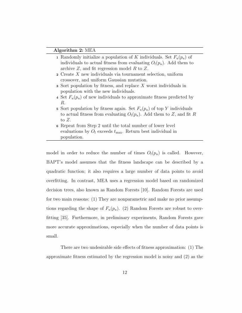
Algorithm 2: MEA

1 Randomly initialize a population of K individuals. Set Fu(pu) ofindividuals to actual fitness from evaluating Ol(pu). Add them toarchive Z, and fit regression model R to Z.

2 Create X new individuals via tournament selection, uniformcrossover, and uniform Gaussian mutation.

3 Sort population by fitness, and replace X worst individuals inpopulation with the new individuals.

4 Set Fu(pu) of new individuals to approximate fitness predicted byR.

5 Sort population by fitness again. Set Fu(pu) of top Y individualsto actual fitness from evaluating Ol(pu). Add them to Z, and fit Rto Z.

6 Repeat from Step 2 until the total number of lower levelevaluations by Ol exceeds tmax. Return best individual inpopulation.

model in order to reduce the number of times Ol(pu) is called. However,

BAPT’s model assumes that the fitness landscape can be described by a

quadratic function; it also requires a large number of data points to avoid

overfitting. In contrast, MEA uses a regression model based on randomized

decision trees, also known as Random Forests [10]. Random Forests are used

for two main reasons: (1) They are nonparametric and make no prior assump-

tions regarding the shape of Fu(pu). (2) Random Forests are robust to over-

fitting [35]. Furthermore, in preliminary experiments, Random Forests gave

more accurate approximations, especially when the number of data points is

small.

There are two undesirable side effects of fitness approximation: (1) The

approximate fitness estimated by the regression model is noisy and (2) as the

12

dimensionality of pu increases, the archive Z and population K must increase

to avoid overfitting. For example in BAPT, which uses regression model R to

fit pu directly, K must increase quadratically with the dimension of pu [37],

which makes it difficult to scale up the approach.

To deal with issue (1), Step 5 is included in MEA to ensure that the

actual fitness of promising but approximately evaluated individuals is always

known. In addition, MEA deals with issue (2) by replacing pu with perfor-

mance metrics that remain fixed in dimensionality. The lower level fitness

function, Ol(pu), is run for roughly fmax

α(α > 1) evaluations and the following

six metrics mu regarding the population of Ol are collected: (1) best fitness,

(2) average fitness, (3) fitness standard deviation, (4) population diversity, (5)

increase in average fitness over last 10 generations and (6) exact number of

function evaluations, which can vary depending on K. Finally, R is fitted

using the mu and actual fitness of individuals in Z, averaged over q runs. The

metrics mu can be used to predict the performance of Ol(pu) since there is usu-

ally strong correlation between an algorithm’s initial and final performance.

Because the size of mu is independent of pu, MEA has no problems dealing

with high-dimensional pu.

As an additional way of smoothing noise, if an upper level individual

remains in the population for multiple generations, its fitness is averaged over

multiple evaluations. Constraints for pu are enforced by clipping them to

the desired minimum and maximum values after mutation is performed. The

archive Z has a maximum size to limit the computational costs of fitting

13

R and when it is full, the newly added individuals replace the oldest ones.

MEA terminates automatically when the total number of lower level fitness

evaluations by Ol exceeds tmax and returns the pu with highest fitness. If there

is a tie, the individual that remained longest in the population is returned.

3.2 Evolving an Adaptive Genetic Algorithm with MEA

In NE, the GA that evolves the neural network is static; the parameters

of the GA do not change between generations during a run. An adaptive GA

(AGA) that is tunable with MEA can be created by modifying a static GA as

follows:

At the beginning of each generation, four metrics regarding the popula-

tion are collected: (1) best fitness in population, (2) mean fitness in population,

(3) standard deviation of population fitnesses, and (4) growth in mean fitness

over the past five generations. A feedforward neural network (also evolved,

but unrelated to controller being evolved in Fl) with four input units, three

hidden units, two output units, and sigmoid activation functions is then ac-

tivated using the metrics as input. The outputs of the network are used to

set the mutation amount and crossover rate of AGA for that generation. By

setting AGA as the lower level Ol in MEA, the weights of the parameter set-

ting neural network can be evolved simultaneously with the remaining static

parameters (population size, replacement rate, etc). A step by step overview

of AGA is given by Algorithm 3.

One issue with using neural networks is that the input must be in a

14

Algorithm 3: AGA

1 Initialize population with K random individuals.2 Evaluate fitness of all individuals in population on some

fitness/objective function.3 Collect metrics regarding state of the population.4 Feed metrics as input to neural network and use output of neural

network to set mutation amount and crossover rate.5 Select high fitness individuals Ih from population.6 Create X new individuals In from Ih through application of

mutation and crossover.7 Replace X low fitness individuals Il with In.8 Repeat from Step 2 until a termination criterion is reached.

reasonable range to avoid saturation of the neurons. This problem is addressed

in AGA by log-scaling the fitnesses of all individuals in the population and

subtracting a bias term equal to the minimum fitness in population to avoid

negative fitness values.

In the next chapter, the performance of MEA will be evaluated on a

diverse variety of test problems, including complex real-world control tasks

and a set of blackbox benchmark functions.

15

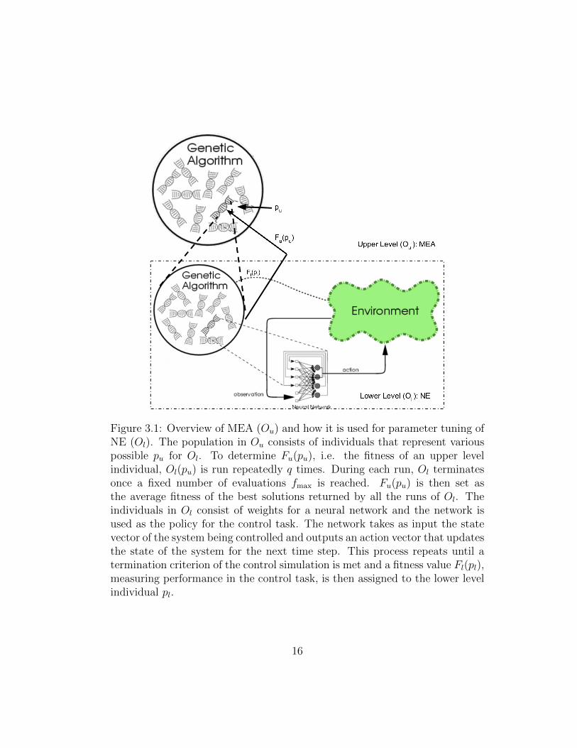
Figure 3.1: Overview of MEA (Ou) and how it is used for parameter tuning ofNE (Ol). The population in Ou consists of individuals that represent variouspossible pu for Ol. To determine Fu(pu), i.e. the fitness of an upper levelindividual, Ol(pu) is run repeatedly q times. During each run, Ol terminatesonce a fixed number of evaluations fmax is reached. Fu(pu) is then set asthe average fitness of the best solutions returned by all the runs of Ol. Theindividuals in Ol consist of weights for a neural network and the network isused as the policy for the control task. The network takes as input the statevector of the system being controlled and outputs an action vector that updatesthe state of the system for the next time step. This process repeats until atermination criterion of the control simulation is met and a fitness value Fl(pl),measuring performance in the control task, is then assigned to the lower levelindividual pl.

16

Chapter 4

Experimental Results

4.1 Experiment Setup

In order to evaluate the performance of MEA, it is compared against

two other EAs designed for parameter tuning on two real-world control tasks.

The first one is SMEA, a simplified version of MEA that does not perform

any fitness function approximation. Thus, instead of performing Steps 4 and

5, the actual fitness of every individual in the population is evaluated before

proceeding to the next generation. The second EA is a version of BAPT

designed for comparison with MEA and thus named BAPTM; it has the same

localized quadratic approximation scheme as BAPT but uses MEA’s uniform

crossover in place of PCX crossover [36]. Uniform crossover is a commonly

used operator that is shown to be effective in many domains [38, 40], including

preliminary experiments in double pole balancing and helicopter hovering. For

all experiments except where indicated, these are the parameters that MEA

uses: the maximum size of Z is set to 100K, K = 20, X = K/2, Y = K/2

and α = 4. Because of an elitist replacement scheme and constraints on pu, a

high mutation rate of 0.5 can be utilized, along with a crossover rate of 0.5.

As mentioned in the introduction, NE is utilized as the lower level Ol since it

is well suited for finding robust, efficient solutions to difficult control problems

17

Figure 4.1: The double pole balancing task. The system consists of two verticalpoles with different lengths that are attached to a movable cart with one degreeof freedom. The goal is to apply a force to the cart at regular time intervals toensure that both poles remain upright and that the cart remains within fixeddistance of its starting position. The six state variables of the system are theangular position and velocities of the poles, as well as the position and velocityof the cart. The fitness of the controller (Fl) is ts, the number of time stepsit can prevent either pole from falling over or the cart from straying too faraway. A pole balancing episode/evaluation is terminated when ts = 100, 000or when failure occurs. Double pole balancing is a good benchmark problemdue to its adjustable difficulty and similarity to many other control tasks.

[2, 20, 28, 42].

4.2 MEA in Double Pole Balancing

Pole balancing, or inverted pendulum, has long been a standard bench-

mark for control algorithms [7, 8, 18, 44]. It is easy to describe and is a

surrogate for other real-world control problems such as finless rocket stabi-

lization. While the original version with a single pole is too easy for modern

methods, the double-pole version can be made arbitrarily hard, and thus serves

as a good first benchmark for bilevel optimization. A summary of the double

18

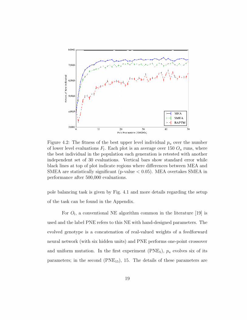
Figure 4.2: The fitness of the best upper level individual pu over the numberof lower level evaluations Fl. Each plot is an average over 150 Ou runs, wherethe best individual in the population each generation is retested with anotherindependent set of 30 evaluations. Vertical bars show standard error whileblack lines at top of plot indicate regions where differences between MEA andSMEA are statistically significant (p-value < 0.05). MEA overtakes SMEA inperformance after 500,000 evaluations.

pole balancing task is given by Fig. 4.1 and more details regarding the setup

of the task can be found in the Appendix.

For Ol, a conventional NE algorithm common in the literature [19] is

used and the label PNE refers to this NE with hand-designed parameters. The

evolved genotype is a concatenation of real-valued weights of a feedforward

neural network (with six hidden units) and PNE performs one-point crossover

and uniform mutation. In the first experiment (PNE5), pu evolves six of its

parameters; in the second (PNE15), 15. The details of these parameters are

19

Figure 4.3: The fitness of the best pu over the number of evaluations of Fl fordifferent values of q with MEA. The data is gathered in the same manner asFig. 4.2. Lower values of q result in better performance, suggesting that MEAis surprisingly robust against evaluation noise.

given in the Appendix.

For PNE5, the following parameters are set for each Ou: q = 1, fmax =

2, 000, and tmax = 5, 000, 000. K = 26 is used for BAPTM as the mini-

mum population size required for optimizing the six parameters of pu [37]. In

Fig. 4.2, the performance of all three Ou with PNE5 as Ol are compared. MEA

achieves statistically significant higher fitness than SMEA after approximately

500,000 lower level evaluations; both are significantly better than BAPTM in

both metrics. Fig. 4.3 shows how the performance of MEA is affected by dif-

ferent values of q, the number of times Ol(pu) is evaluated. Interestingly, lower

values of q result in faster learning with no difference in peak fitness achieved.

20

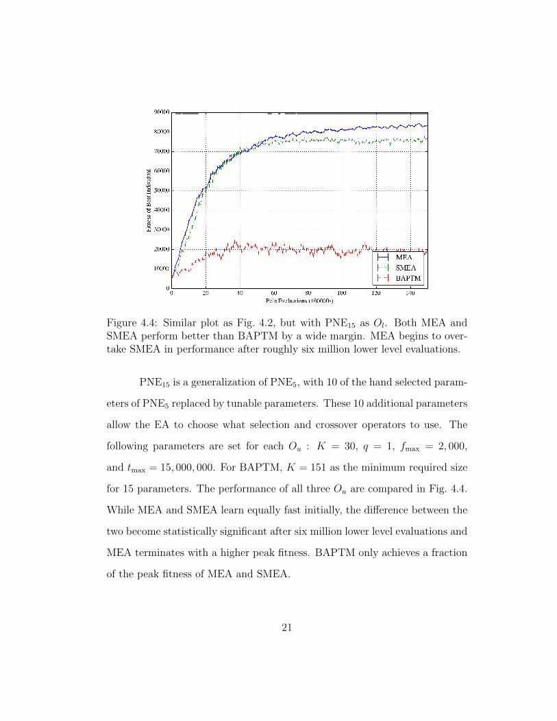
Figure 4.4: Similar plot as Fig. 4.2, but with PNE15 as Ol. Both MEA andSMEA perform better than BAPTM by a wide margin. MEA begins to over-take SMEA in performance after roughly six million lower level evaluations.

PNE15 is a generalization of PNE5, with 10 of the hand selected param-

eters of PNE5 replaced by tunable parameters. These 10 additional parameters

allow the EA to choose what selection and crossover operators to use. The

following parameters are set for each Ou : K = 30, q = 1, fmax = 2, 000,

and tmax = 15, 000, 000. For BAPTM, K = 151 as the minimum required size

for 15 parameters. The performance of all three Ou are compared in Fig. 4.4.

While MEA and SMEA learn equally fast initially, the difference between the

two become statistically significant after six million lower level evaluations and

MEA terminates with a higher peak fitness. BAPTM only achieves a fraction

of the peak fitness of MEA and SMEA.

21

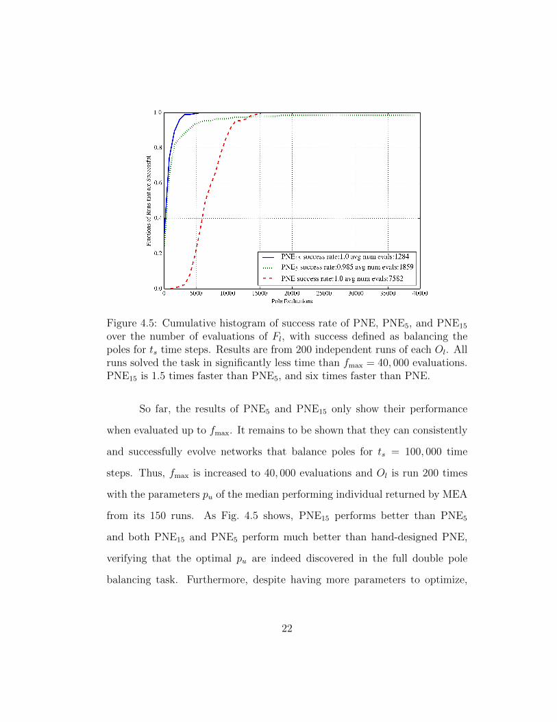
Figure 4.5: Cumulative histogram of success rate of PNE, PNE5, and PNE15

over the number of evaluations of Fl, with success defined as balancing thepoles for ts time steps. Results are from 200 independent runs of each Ol. Allruns solved the task in significantly less time than fmax = 40, 000 evaluations.PNE15 is 1.5 times faster than PNE5, and six times faster than PNE.

So far, the results of PNE5 and PNE15 only show their performance

when evaluated up to fmax. It remains to be shown that they can consistently

and successfully evolve networks that balance poles for ts = 100, 000 time

steps. Thus, fmax is increased to 40, 000 evaluations and Ol is run 200 times

with the parameters pu of the median performing individual returned by MEA

from its 150 runs. As Fig. 4.5 shows, PNE15 performs better than PNE5

and both PNE15 and PNE5 perform much better than hand-designed PNE,

verifying that the optimal pu are indeed discovered in the full double pole

balancing task. Furthermore, despite having more parameters to optimize,

22

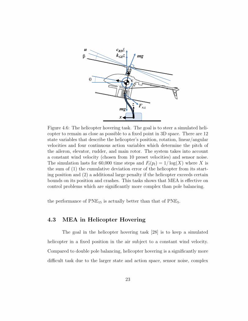
Figure 4.6: The helicopter hovering task. The goal is to steer a simulated heli-copter to remain as close as possible to a fixed point in 3D space. There are 12state variables that describe the helicopter’s position, rotation, linear/angularvelocities and four continuous action variables which determine the pitch ofthe aileron, elevator, rudder, and main rotor. The system takes into accounta constant wind velocity (chosen from 10 preset velocities) and sensor noise.The simulation lasts for 60,000 time steps and Fl(pl) = 1/ log(X) where X isthe sum of (1) the cumulative deviation error of the helicopter from its start-ing position and (2) a additional large penalty if the helicopter exceeds certainbounds on its position and crashes. This tasks shows that MEA is effective oncontrol problems which are significantly more complex than pole balancing.

the performance of PNE15 is actually better than that of PNE5.

4.3 MEA in Helicopter Hovering

The goal in the helicopter hovering task [28] is to keep a simulated

helicopter in a fixed position in the air subject to a constant wind velocity.

Compared to double pole balancing, helicopter hovering is a significantly more

difficult task due to the larger state and action space, sensor noise, complex

23

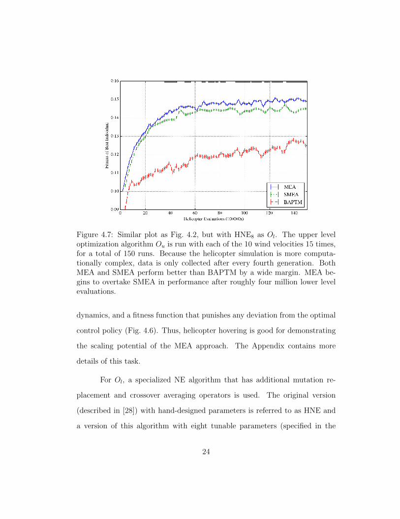
Figure 4.7: Similar plot as Fig. 4.2, but with HNE8 as Ol. The upper leveloptimization algorithm Ou is run with each of the 10 wind velocities 15 times,for a total of 150 runs. Because the helicopter simulation is more computa-tionally complex, data is only collected after every fourth generation. BothMEA and SMEA perform better than BAPTM by a wide margin. MEA be-gins to overtake SMEA in performance after roughly four million lower levelevaluations.

dynamics, and a fitness function that punishes any deviation from the optimal

control policy (Fig. 4.6). Thus, helicopter hovering is good for demonstrating

the scaling potential of the MEA approach. The Appendix contains more

details of this task.

For Ol, a specialized NE algorithm that has additional mutation re-

placement and crossover averaging operators is used. The original version

(described in [28]) with hand-designed parameters is referred to as HNE and

a version of this algorithm with eight tunable parameters (specified in the

24

Figure 4.8: The fitness of the best individual over the number of evaluationsof Fl by HNE and HNE8. Results are averaged over 500 runs, with 50 runs foreach of the 10 wind velocities. HNE8 both learns faster and achieves higherpeak fitness than HNE.

Appendix), is referred to as HNE8. The network evolved by HNE has a

hand-designed topology and consists of 11 linear and sigmoid hidden units

[28]. The following parameters are set for each Ou: q = 1, fmax = 5, 000,

and tmax = 15, 000, 000; for BAPTM, K = 51. As seen in Fig. 4.7, the per-

formance improvement of MEA over SMEA becomes statistically significant

after roughly four million evaluations and both are significantly better than

BAPTM. Fig. 4.8 compares the performance of representative examples (me-

dian performing individual for each wind velocity) of HNE8 and HNE when the

task is solved fully with fmax = 25, 000. In comparison to HNE, HNE8 learns

faster and achieves higher peak fitness, demonstrating the value of bilevel op-

25

timization over hand-design.

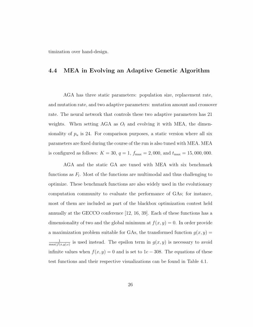
4.4 MEA in Evolving an Adaptive Genetic Algorithm

AGA has three static parameters: population size, replacement rate,

and mutation rate, and two adaptive parameters: mutation amount and crossover

rate. The neural network that controls these two adaptive parameters has 21

weights. When setting AGA as Ol and evolving it with MEA, the dimen-

sionality of pu is 24. For comparison purposes, a static version where all six

parameters are fixed during the course of the run is also tuned with MEA. MEA

is configured as follows: K = 30, q = 1, fmax = 2, 000, and tmax = 15, 000, 000.

AGA and the static GA are tuned with MEA with six benchmark

functions as Fl. Most of the functions are multimodal and thus challenging to

optimize. These benchmark functions are also widely used in the evolutionary

computation community to evaluate the performance of GAs; for instance,

most of them are included as part of the blackbox optimization contest held

annually at the GECCO conference [12, 16, 39]. Each of these functions has a

dimensionality of two and the global minimum at f(x, y) = 0. In order provide

a maximization problem suitable for GAs, the transformed function g(x, y) =

1max(f(x,y),ε)

is used instead. The epsilon term in g(x, y) is necessary to avoid

infinite values when f(x, y) = 0 and is set to 1e− 308. The equations of these

test functions and their respective visualizations can be found in Table 4.1.

26

Name and Equation Visualization

Dejong F5

f(x, y) =(0.002 +

∑25i=1

1i+(x1−a1i)6+(x2−a2i)6

)−1

a =

(−32 −16 0 16 32 −32 ... 32−32 −32 −32 −32 −32 −16 ... 32

)

Schaffer F6

f(x, y) = 0.5 +sin2(

√x2+y2)−0.5

[1+0.001·(x2+y2)]2

Schaffer F7

f(x0 · · ·xn) = [ 1n−1

√si · (sin(50.0s

15i ) + 1)]2

si +√x2i + x2i+1

Rosenbrockf(x1 · · ·xn) =

∑n−1i=1 (100(x2i − xi+1)

2 + (1− xi)2)

Rastriginf(x1 · · ·xn) = 10n+

∑ni=1(x

2i − 10cos(2πxi))

Schwefelf(x1 · · ·xn) =

∑ni=1(−xisin(

√|xi|)) + α · n

α = 418.982887

Table 4.1: Names, equations, and visualizations of the six optimization bench-mark functions that are used to evaluate the performance of AGA.

27

As shown by Fig. 4.9, MEA evolves an AGA that easily exceeds the

performance of the static GA for all six test functions. In some cases the

performance difference can be quite large, as seen in Fig. 4.9(f). The main

reason is that the function being optimized is g(x, y) = 1max(f(x,y),ε)

; the closer

f(x, y) gets to zero, the closer g(x, y) becomes to 1ε. As a result, small decreases

in f(x, y) near its minimum will translate into large increases in g(x, y).

In Fig. 4.10, the behavior of AGA is visualized for each of the six

functions. The plots on the odd and even columns show how the mutation

amount and crossover rate vary over the generations, respectively. Results

are averaged over 1500 runs of AGA (10 runs for each evolved pu returned

by MEA). The shaded error regions in the plots of each adaptive parameter

show the standard deviation. The visualizations indicate a clear pattern in the

adaption of the mutation amount: it starts high and steadily decreases over

the generations. On the other hand, no clear pattern exists for the crossover

rate.

The next chapter will analyze the results from experiments in more de-

tail, present interesting findings, and describe possible areas of future research.

28

(a) (b)

(c) (d)

(e) (f)

Figure 4.9: Comparison of the performance of the adaptive (blue line) andstatic (green line) GA as Ol and with (a) Dejong F5, (b) Schaffer F6, (c)Schaffer F7, (d) Rosenbrock, (e) Rastrigin, and (f) Schwefel as Fl. AGA showsnoticeable improvement in performance over the static version.

29

(a) (b)

(c) (d)

(e) (f)

Figure 4.10: Visualization of how AGA changes the mutation amount (oddcolumns) and crossover rate (even columns) for (a) Dejong F5, (b) SchafferF6, (c) Schaffer F7, (d) Rosenbrock, (e) Rastrigin, and (f) Schwefel as Fl.The x-axis shows the number of generations elapsed while the y-axis showsthe magnitude of the adaptive parameters. Shaded error regions shows thestandard deviation. For all six functions, there is a clear trend where themutation amount decreases over time. There is no evident pattern for crossoverrate.

30

Chapter 5

Discussion and Future Work

The experimental results in the previous chapter reveal some interesting

findings regarding MEA and its applications to optimizing control tasks and

benchmark functions. They also suggest interesting areas for further research.

5.1 Analysis of Experimental Results

The results from the experiments show that MEA performs better than

SMEA and that both are much better than BAPTM. The main cause of

BAPTM’s performance are the inaccurate approximations given by its re-

gression model. The relatively few number of individuals in Z during the first

generations and noise in evaluating Ol(pu) cause the quadratic model to overfit

initially. Furthermore, the fitness landscape of Fu is irregular and not well de-

scribed by a quadratic approximation. For example, preliminary experiments

show that doubling the population size of PNE5 can result in Fu(pu) decreasing

by an order of magnitude.

Surprisingly, running MEA with lower values of q results in better per-

formance and faster convergence to the optimal fitness value. This result is

counter-intuitive because there is more evaluation noise with smaller values

31

of q and some averaging of evaluations should be useful. One explanation is

that as the number of generations increase, both the fitness averaging and

approximation mechanisms of MEA become more accurate. They eventually

help smooth out the evaluation noise, retaining individuals with good fitness,

and eliminating those with bad fitness. This conclusion is supported by ob-

servations that the performance of MEA becomes steadily less noisy and more

consistent over the generations. As seen in Figs. 4.2, 4.4, and 4.7, MEA’s fit-

ness approximation mechanism also explains why its performance continues to

increase even though that of SMEA, which does not use fitness approximation,

is flattening out.

Interestingly, although PNE15 has three times as many pu as PNE5, the

performance of PNE15 is noticeably better. A more complex parameterization

of an optimization algorithm allows it to fit better to a problem, especially if

it is using parameters discovered through bilevel optimization. With MEA,

it might thus be possible to discover specialized optimization algorithms that

excel in solving particular problem domains.

The results of evolving AGA are promising on a selection of standard

benchmark functions for blackbox optimization. The tendency for mutation

amount to decrease resembles the behavior of hand-tuned adaptive GAs in

literature [41]. As the population moves closer to the optimum of the fitness

function, a decrease in the mutation amount makes sense since it increases the

probability that the newly created individuals will remain near the optimum

and not deviate too far off. The lack of a clear pattern for crossover rate may

32

suggest that the effectiveness of crossover may not depend on the current state

of the population or how close the population is to the optimum.

There are still some limitations to what AGA can achieve. Prelimi-

nary experimental results show that evolving AGA offers no performance im-

provement over a static GA in the domain of a real-world problem such as

double-pole balancing. The lack of any performance difference suggests that

the fitness function for NE is fundamentally different from test functions. It

is also possible that the optimal behavior for the GA parameters in NE is to

simply remain the same over the generations. Another limitation is that AGA

is not invariant to changes in the scaling of the fitness function. For exam-

ple, if AGA is tuned over f(x, y), it might output different and possibly worst

performing adaptive parameters for 100f(x, y). The reason is that the input

to the neural network which sets the parameters every generation will also be

increased by a factor of 100, thus causing the neurons to saturate.

5.2 Future Work

There are several interesting directions of future work:

1. Further research in evolving AGAs for neuroevolution tasks. This re-

search includes trying more state features and normalization schemes

for the parameter setting neural network and having that network set

other parameters such as population size.

2. Optimizing not only the learning parameters of NE at the upper level,

33

but also the topology of the neural network. This is reminiscent of

Whiteson and Stone’s NEAT+Q algorithm [43] where an upper level EA

evolves the topology of a neural network value-function approximator

and its weights are fined-tuned with backpropagation as Ol. There has

been much research recently into training deep neural networks for tasks

like image recognition and classification. In almost all cases, the topol-

ogy of the neural network and the learning parameters are selected by

hand, yet it has been acknowledged that both make a huge impact on the

performance. It would be interesting to see if a bilevel approach can dis-

cover deep neural networks that can exceed state of the art performance

on image classification datasets.

3. Combining various heuristics from existing EAs, such as differential evo-

lution and particle swarm optimization, to create a more complex and

general-purpose lower level parameterization that performs well on a

wide variety of optimization problems.

34

Chapter 6

Conclusion

In this thesis, parameter tuning for NE is cast as a bilevel optimization

problem. A novel upper level optimization algorithm, MEA, is proposed and

shown to achieve better results in optimizing parameters for NE. These evolved

parameters result in significantly better performance over hand-designed ones

in two difficult real-world control tasks. Remarkably, evolving a more complex

parameterization of the lower level optimization algorithm results in better

performance, even though such a parameterization would be very difficult to

manage by hand. Lastly, MEA has been shown to be capable of evolving an

AGA that outperforms static GAs on certain benchmark functions. Bilevel

optimization is thus a promising approach for solving a variety of difficult

optimization problems.

35

Chapter 7

Appendix

The Appendix contains more details regarding the two control tasks

and lower level optimization algorithms Ol that are used in the experiments

to evaluate the performance of MEA.

7.1 Details of Control Tasks

For the double pole balancing task, the length and mass of the longer

pole is set to 0.5 meters and 0.1 kilogram. The length and mass of the shorter

pole is set to 0.05 meters and 0.01 kilograms. The mass of the cart itself is 1.0

kilogram. The shorter pole is initialized in a vertical position while the longer

pole is initialized with one degree offset from the shorter pole. Both poles

and the cart have zero initial velocity. The topology of the neural network

controller whose weights are evolved by PNE5 and PNE15 is shown in Fig. 7.2.

For the helicopter hovering task, the linear equations that describe the

dynamics of the helicopter simulator is given in detail in [28]. The topology

of the controller whose weights are evolved by HNE8 is shown in Fig. 7.2.

The wind speeds in the simulator are fixed and within the range of [−5, 5] m

for both the X-axis and the Y-axis. The helicopter crashes when one of the

36

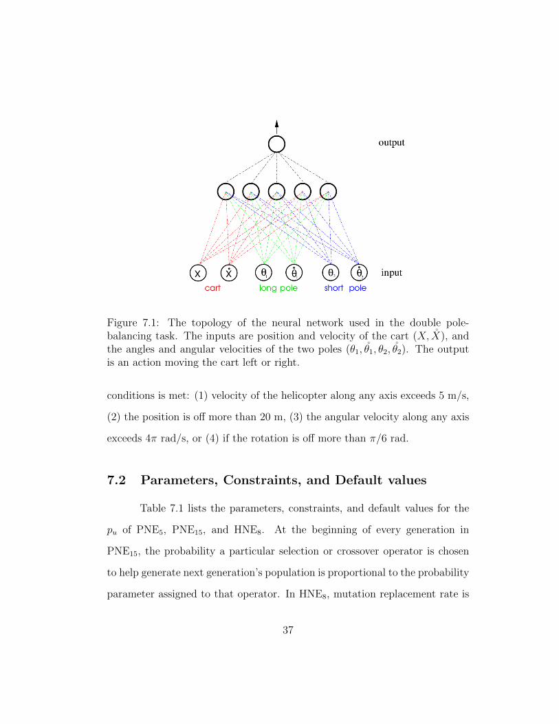
Figure 7.1: The topology of the neural network used in the double pole-balancing task. The inputs are position and velocity of the cart (X, X), andthe angles and angular velocities of the two poles (θ1, θ1, θ2, θ2). The outputis an action moving the cart left or right.

conditions is met: (1) velocity of the helicopter along any axis exceeds 5 m/s,

(2) the position is off more than 20 m, (3) the angular velocity along any axis

exceeds 4π rad/s, or (4) if the rotation is off more than π/6 rad.

7.2 Parameters, Constraints, and Default values

Table 7.1 lists the parameters, constraints, and default values for the

pu of PNE5, PNE15, and HNE8. At the beginning of every generation in

PNE15, the probability a particular selection or crossover operator is chosen

to help generate next generation’s population is proportional to the probability

parameter assigned to that operator. In HNE8, mutation replacement rate is

37

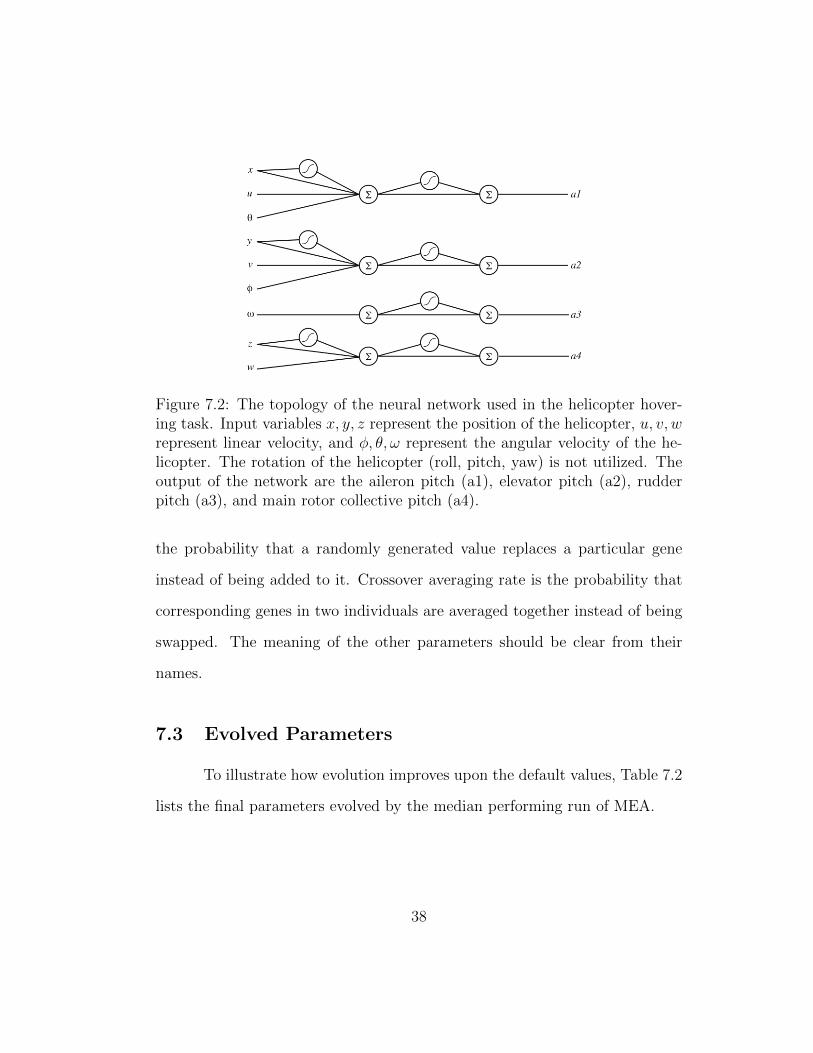
Figure 7.2: The topology of the neural network used in the helicopter hover-ing task. Input variables x, y, z represent the position of the helicopter, u, v, wrepresent linear velocity, and φ, θ, ω represent the angular velocity of the he-licopter. The rotation of the helicopter (roll, pitch, yaw) is not utilized. Theoutput of the network are the aileron pitch (a1), elevator pitch (a2), rudderpitch (a3), and main rotor collective pitch (a4).

the probability that a randomly generated value replaces a particular gene

instead of being added to it. Crossover averaging rate is the probability that

corresponding genes in two individuals are averaged together instead of being

swapped. The meaning of the other parameters should be clear from their

names.

7.3 Evolved Parameters

To illustrate how evolution improves upon the default values, Table 7.2

lists the final parameters evolved by the median performing run of MEA.

38

PNE5 Parameters Constraints DefaultMutation Rate [0,1] 0.40Mutation Amount [0,1] 0.30Replacement Fraction [0,1] 0.50Initial Weight Range [0,12] 6.00Population Size [0,400] 400Extra PNE15 Parameters Constraints DefaultMutation Probability [0,1] 1.00Crossover Probability [0,1] 1.00Uniform Crossover Rate [0,1] 0.00Tournament/Truncation Fraction [0,1] 0.25Tournament Selection Probability [0,1] 0.00Truncation Selection Probability [0,1] 1.00Roulette Selection Probability [0,1] 0.001-pt Crossover Probability [0,1] 1.002-pt Crossover Probability [0,1] 0.00Uniform Crossover Probability [0,1] 0.00HNE8 Parameters Constraints DefaultMutation Probability [0,1] 0.75Mutation Rate [0,1] 0.10Mutation Amount [0,1] 0.80Mutation Replacement Rate [0,1] 0.25Replacement Fraction [0,1] 0.02Population Size [0,200] 50Crossover Probability [0,1] 0.50Crossover Averaging Rate [0,1] 0.50

Table 7.1: Parameters, constraints, and default values for PNE5, PNE15, andHNE8.

39

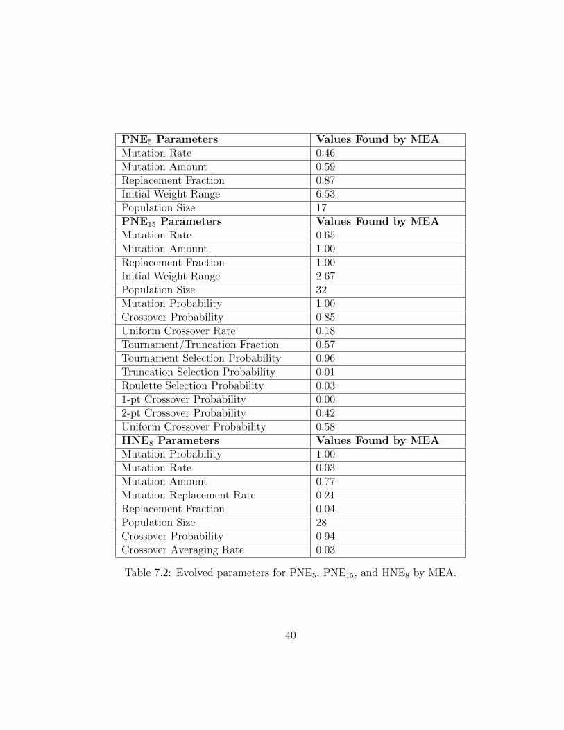
PNE5 Parameters Values Found by MEAMutation Rate 0.46Mutation Amount 0.59Replacement Fraction 0.87Initial Weight Range 6.53Population Size 17PNE15 Parameters Values Found by MEAMutation Rate 0.65Mutation Amount 1.00Replacement Fraction 1.00Initial Weight Range 2.67Population Size 32Mutation Probability 1.00Crossover Probability 0.85Uniform Crossover Rate 0.18Tournament/Truncation Fraction 0.57Tournament Selection Probability 0.96Truncation Selection Probability 0.01Roulette Selection Probability 0.031-pt Crossover Probability 0.002-pt Crossover Probability 0.42Uniform Crossover Probability 0.58HNE8 Parameters Values Found by MEAMutation Probability 1.00Mutation Rate 0.03Mutation Amount 0.77Mutation Replacement Rate 0.21Replacement Fraction 0.04Population Size 28Crossover Probability 0.94Crossover Averaging Rate 0.03

Table 7.2: Evolved parameters for PNE5, PNE15, and HNE8 by MEA.

40

Bibliography

[1] B. Adenso-Diaz and M. Laguna. “Fine-tuning of algorithms using frac-tional experimental designs and local search”. In: Operations Research54.1 (2006), pp. 99–114.

[2] B. F. Allen and P. Faloutsos. “Evolved controllers for simulated locomo-tion”. In: Motion in Games. Springer, 2009, pp. 219–230.

[3] C. Ansotegui, M. Sellmann, and K. Tierney. “A gender-based geneticalgorithm for the automatic configuration of algorithms”. In: Princi-ples and Practice of Constraint Programming-CP 2009. Springer, 2009,pp. 142–157.

[4] K. J. Astrom and T. Hagglund. Advanced PID control. ISA-The Instru-mentation, Systems, and Automation Society; Research Triangle Park,NC 27709, 2006.

[5] J. A. Bagnell and J. G. Schneider. “Autonomous helicopter control usingreinforcement learning policy search methods”. In: Robotics and Automa-tion, 2001. Proceedings 2001 ICRA. IEEE International Conference on.Vol. 2. IEEE. 2001, pp. 1615–1620.

[6] L. Baird and A. W. Moore. “Gradient descent for general reinforcementlearning”. In: Advances in neural information processing systems (1999),pp. 968–974.

[7] A. G. Barto. Reinforcement learning: An introduction. MIT press, 1998.

[8] H. R. Berenji and P. Khedkar. “Learning and tuning fuzzy logic con-trollers through reinforcements”. In: Neural Networks, IEEE Transac-tions on 3.5 (1992), pp. 724–740.

41

[9] M. Birattari et al. “F-Race and iterated F-Race: An overview”. In: Ex-perimental methods for the analysis of optimization algorithms. Springer,2010, pp. 311–336.

[10] L. Breiman. “Random forests”. In: Machine learning 45.1 (2001), pp. 5–32.

[11] L. Davis et al. Handbook of genetic algorithms. Vol. 115. Van NostrandReinhold New York, 1991.

[12] J. M. Dieterich and B. Hartke. “Empirical review of standard benchmarkfunctions using evolutionary global optimization”. In: arXiv preprintarXiv:1207.4318 (2012).

[13] L. S. Diosan and M. Oltean. “Evolving evolutionary algorithms usingevolutionary algorithms”. In: Proceedings of the 2007 GECCO confer-ence companion on Genetic and evolutionary computation. ACM. 2007,pp. 2442–2449.

[14] A. Eiben et al. “Reinforcement learning for online control of evolutionaryalgorithms”. In: Engineering Self-Organising Systems. Springer, 2007,pp. 151–160.

[15] A. E. Eiben and S. K. Smit. “Parameter tuning for configuring andanalyzing evolutionary algorithms”. In: Swarm and Evolutionary Com-putation 1.1 (2011), pp. 19–31.

[16] S. Finck et al. Real-parameter black-box optimization benchmarking 2009:Presentation of the noiseless functions. Tech. rep. Citeseer, 2010.

[17] D. Floreano, P. Durr, and C. Mattiussi. “Neuroevolution: from archi-tectures to learning”. In: Evolutionary Intelligence 1.1 (2008), pp. 47–62.

[18] F. Gomez, J. Schmidhuber, and R. Miikkulainen. “Accelerated neuralevolution through cooperatively coevolved synapses”. In: The Journalof Machine Learning Research 9 (2008), pp. 937–965.

42

[19] F. Gomez, J. Schmidhuber, and R. Miikkulainen. “Efficient non-linearcontrol through neuroevolution”. In: Machine Learning: ECML 2006.Springer, 2006, pp. 654–662.

[20] F. J. Gomez and R. Miikkulainen. “Active guidance for a finless rocketusing neuroevolution”. In: Genetic and Evolutionary Computation-GECCO2003. Springer. 2003, pp. 2084–2095.

[21] F. J. Gomez and R. Miikkulainen. Robust non-linear control throughneuroevolution. Computer Science Department, University of Texas atAustin, 2003.

[22] J. J. Grefenstette. “Optimization of control parameters for genetic algo-rithms”. In: Systems, Man and Cybernetics, IEEE Transactions on 16.1(1986), pp. 122–128.

[23] J. J. Grefenstette, D. E. Moriarty, and A. C. Schultz. “Evolutionary al-gorithms for reinforcement learning”. In: arXiv preprint arXiv:1106.0221(2011).

[24] F. Hutter, H. H. Hoos, and K. Leyton-Brown. “Sequential model-basedoptimization for general algorithm configuration”. In: Learning and In-telligent Optimization. Springer, 2011, pp. 507–523.

[25] F. Hutter et al. “ParamILS: an automatic algorithm configuration frame-work”. In: Journal of Artificial Intelligence Research 36.1 (2009), pp. 267–306.

[26] Y. Jin. “A comprehensive survey of fitness approximation in evolutionarycomputation”. In: Soft computing 9.1 (2005), pp. 3–12.

[27] N. Kohl and P. Stone. “Policy gradient reinforcement learning for fastquadrupedal locomotion”. In: Robotics and Automation, 2004. Proceed-ings. ICRA’04. 2004 IEEE International Conference on. Vol. 3. IEEE.2004, pp. 2619–2624.

43

[28] R. Koppejan and S. Whiteson. “Neuroevolutionary reinforcement learn-ing for generalized control of simulated helicopters”. In: Evolutionaryintelligence 4.4 (2011), pp. 219–241.

[29] O. Kramer. “Evolutionary self-adaptation: a survey of operators andstrategy parameters”. In: Evolutionary Intelligence 3.2 (2010), pp. 51–65.

[30] J. Lehman and R. Miikkulainen. “Neuroevolution”. In: Scholarpedia8.6 (2013), p. 30977. url: http://nn.cs.utexas.edu/?lehman:

scholarpedia13.

[31] R. Myers and E. R. Hancock. “Empirical modelling of genetic algo-rithms”. In: Evolutionary computation 9.4 (2001), pp. 461–493.

[32] V. Nannen and A. E. Eiben. “Relevance Estimation and Value Calibra-tion of Evolutionary Algorithm Parameters.” In: IJCAI. Vol. 7. 2007,pp. 975–980.

[33] I. C. Ramos et al. “Logistic regression for parameter tuning on an evo-lutionary algorithm”. In: Evolutionary Computation, 2005. The 2005IEEE Congress on. Vol. 2. IEEE. 2005, pp. 1061–1068.

[34] A. Ratle. “Accelerating the convergence of evolutionary algorithms byfitness landscape approximation”. In: Parallel Problem Solving from Nature-PPSN V. Springer. 1998, pp. 87–96.

[35] M. Robnik-Sikonja. “Improving random forests”. In: Machine Learning:ECML 2004. Springer, 2004, pp. 359–370.

[36] A. Sinha, A. Srinivasan, and K. Deb. “A population-based, parent centricprocedure for constrained real-parameter optimization”. In: EvolutionaryComputation, 2006. CEC 2006. IEEE Congress on. IEEE. 2006, pp. 239–245.

[37] A. Sinha et al. “A Bilevel Optimization Approach to Automated Param-eter Tuning”. In: (2014).

44

[38] W. M. Spears and K. D. De Jong. On the virtues of parameterized uni-form crossover. Tech. rep. DTIC Document, 1995.

[39] M Srinivas and L. M. Patnaik. “Adaptive probabilities of crossover andmutation in genetic algorithms”. In: Systems, Man and Cybernetics,IEEE Transactions on 24.4 (1994), pp. 656–667.

[40] G. Syswerda. “Uniform crossover in genetic algorithms”. In: (1989).

[41] D. Thierens. “Adaptive mutation rate control schemes in genetic algo-rithms”. In: Evolutionary Computation, 2002. CEC’02. Proceedings ofthe 2002 Congress on. Vol. 1. IEEE. 2002, pp. 980–985.

[42] J. Togelius and S. M. Lucas. “Evolving controllers for simulated carracing”. In: Evolutionary Computation, 2005. The 2005 IEEE Congresson. Vol. 2. IEEE. 2005, pp. 1906–1913.

[43] S. Whiteson and P. Stone. “Evolutionary function approximation forreinforcement learning”. In: The Journal of Machine Learning Research7 (2006), pp. 877–917.

[44] A. P. Wieland. “Evolving neural network controllers for unstable sys-tems”. In: Neural Networks, 1991., IJCNN-91-Seattle International JointConference on. Vol. 2. IEEE. 1991, pp. 667–673.

[45] X. Yao. “Evolving artificial neural networks”. In: Proceedings of theIEEE 87.9 (1999), pp. 1423–1447.

45

Vita

Jason Zhi Liang received his Bachelor’s degree in Electrical Engineering

and Computer Science from the University of California, Berkeley in 2013. As

an undergraduate there, he worked with Avideh Zakhor on Computer Vision

algorithms for image retrieval and localization in indoor environments. He is

currently a Master student in Computer Science under the supervision of Risto

Miikkulainen at the University of Texas at Austin and will graduate in 2015.

Permanent address: 2317 Speedway, Stop D9500Austin, Texas 78712-1757 USA

This thesis was typeset with LATEX† by the author.

†LATEX is a document preparation system developed by Leslie Lamport as a specialversion of Donald Knuth’s TEX Program.

46