copyright by huihui wang 2005 · acknowledgments first of all, i would like to express my sincere...
TRANSCRIPT

Copyright
by
Huihui Wang
2005
The Dissertation Committee for Huihui Wang
certifies that this is the approved version of the following dissertation:
Modeling and Wideband Characterization of Radio
Wave Propagation in Microcells
Committee:
Theodore S. Rappaport, Supervisor
Hao Ling
John H. Davis
Donald S. Fussell
E. Glenn Lightsey

Modeling and Wideband Characterization of Radio
Wave Propagation in Microcells
by
Huihui Wang, B.Sc., M.Eng., M.Sc.
Dissertation
Presented to the Faculty of the Graduate School of
The University of Texas at Austin
in Partial Fulfillment
of the Requirements
for the Degree of
Doctor of Philosophy
The University of Texas at Austin
May 2005

To My Family

Acknowledgments
First of all, I would like to express my sincere gratitude to my advisor, Professor
Theodore S. Rappaport, for his invaluable inspiration, encouragement, guidance and
support throughout my doctoral study. I am also very grateful to Professor Hao
Ling for his insightful expertise advices and many great helps with my research and
graduate study in the past few years. My many thanks to the professors on my
committee, Professor John H. Davis, Professor Donald S. Fussell, and Professor E.
Glenn Lightsey, for their reviewing my work and offering suggestions on my research.
The financial support provided by the National Science Foundation Next Generation
Software research program under the grant number ACI-0305644 and the WNCG
Industrial Affiliation Program are gratefully acknowledged.
My sincere thanks go to Craig Bergstrom at Virginia Tech for his collabo-
ration and help with the S4W software package in the Montage project. Without
his continuous remote help, I would not have been able to plunge into and have a
thorough taste of S4W . My special thanks go to Dr. William Mark Smith from
MIT Lincoln Laboratory for providing valuable measurement data and resourceful
suggestions on my research. Much appreciation is attributed to Dr. Yong Zhou for
always offering help and discussions ever since the early stage of my research.
I would like to express my thanks to all the people in WNCG. I would like to
thank my colleagues Chen Na and Jeremy Chen for their constructive discussions,
various help, vigorous encouragement, and friendships. My sincere thanks go to
v

Jennifer Wright and other staffs for their warmhearted help and support. Special
thanks to Lee Hill for his various help with computer facilities. My appreciation
extends to all my friends and colleagues who have offered their help and spiritual
encouragement during my graduate study.
I am very much indebted to my dear parents and family for their love, en-
couragement and support throughout my educational endeavors. Last, but not least,
I would like to thank my husband Huijie Xu for his love and continuous support
through my graduate study. Standing side by side, our years of stay overseas has
been one of the most memorable periods in my life.
Huihui Wang
The University of Texas at Austin
May 2005
vi

Modeling and Wideband Characterization of Radio
Wave Propagation in Microcells
Publication No.
Huihui Wang, Ph.D.
The University of Texas at Austin, 2005
Supervisor: Theodore S. Rappaport
This dissertation focuses on radio wave propagation prediction modeling in micro-
cellular environments. Mathematical modeling techniques and channel characteri-
zation have been addressed. The research begins with a survey of ray-tracing based
propagation prediction modeling methods and the evolution of diffraction modeling,
and makes three new contributions.
First, diffraction theory has been used to enhance the accuracy in shadowed
regions for ray-tracing algorithms by a novel, computationally fast approach. A
parametric formulation of the UTD diffraction coefficient has been proposed us-
ing the inverse problem theory. Significant improvement in the estimation of the
diffracted field for right-angle dielectric wedges is achieved over existing heuristic
vii

methods. This construction offers a faster estimation of the diffracted field and is
suitable for real-time wireless channel estimation. The diffraction modeling method
has been applied in indoor and outdoor environments to expedite propagation pre-
diction.
Next, the ray-tracing prediction modeling method developed on the NSF
Montage project is applied and validated with published measurements at 800 MHz
in the San Francisco financial area to investigate the ability to predict and model
wave propagation in a dense urban environment. Cross-correlation of the predicted
and the measured signal strengths has been calculated at various street intersections
and correlation coefficients of higher than 0.8 are achieved under all circumstances
where corner effect occurs. Further investigations show that the waveguide effect in
the street canyon is only applicable to the propagation phenomena in radial streets
with respect to the transmitter. While in the case of cross streets that are not close
to the transmitter, wave penetration through the building walls makes significant
contribution to signal variations.
Finally, site-specific prediction is applied to the campus of Pickle Research
Center at UT-Austin to study the MIMO channel characteristics. The prediction
using a 4× 8 uniform linear array system operating at 1.8 GHz shows that S4W is
able to reproduce fading statistics and that the estimation of MIMO channel capacity
using ray-tracing method is dependent on the accuracy of the input propagation
environment.
viii

Contents
Acknowledgments v
Abstract vii
List of Tables xiii
List of Figures xiv
Chapter 1 Introduction 1
1.1 Motivation of the Work . . . . . . . . . . . . . . . . . . . . . . . . . 1
1.1.1 Challenges to Current Site-Specific Models . . . . . . . . . . 2
1.1.2 Trend of Site-Specific Radio . . . . . . . . . . . . . . . . . . . 4
1.1.3 Site-Specific Modeling Tools . . . . . . . . . . . . . . . . . . . 6
1.2 Contribution of the Dissertation . . . . . . . . . . . . . . . . . . . . 8
1.3 Organization of the Dissertation . . . . . . . . . . . . . . . . . . . . 9
Chapter 2 Modeling of Propagation Mechanisms 11
2.1 Multipath Propagation . . . . . . . . . . . . . . . . . . . . . . . . . . 12
2.1.1 Free Space Propagation . . . . . . . . . . . . . . . . . . . . . 12
2.1.2 Specular Reflection . . . . . . . . . . . . . . . . . . . . . . . . 14
2.1.3 Transmission . . . . . . . . . . . . . . . . . . . . . . . . . . . 17
2.1.4 Diffraction . . . . . . . . . . . . . . . . . . . . . . . . . . . . 17
ix

2.1.5 Diffuse Scattering . . . . . . . . . . . . . . . . . . . . . . . . 19
2.1.6 Received Ray Power . . . . . . . . . . . . . . . . . . . . . . . 19
2.2 Improvement of Diffraction Modeling . . . . . . . . . . . . . . . . . . 20
2.2.1 GTD Diffraction Coefficient . . . . . . . . . . . . . . . . . . . 22
2.2.2 UTD Diffraction Coefficients . . . . . . . . . . . . . . . . . . 23
2.2.3 Luebbers’ Heuristic Model . . . . . . . . . . . . . . . . . . . . 25
2.2.4 Regional Modification . . . . . . . . . . . . . . . . . . . . . . 26
2.2.5 Comparison and Discussion . . . . . . . . . . . . . . . . . . . 27
2.2.6 Multi-Edge Transition Zone Diffraction . . . . . . . . . . . . 27
2.3 Diffraction in Propagation Prediction . . . . . . . . . . . . . . . . . . 32
2.3.1 Importance of Diffraction in Propagation Prediction . . . . . 32
2.3.2 UTD Propagation Models for Microcellular Communications 33
2.3.3 Challenges to the Prediction of Diffraction . . . . . . . . . . . 34
2.4 Summary . . . . . . . . . . . . . . . . . . . . . . . . . . . . . . . . . 35
Chapter 3 Ray-Tracing Based Site-Specific Modeling 36
3.1 Introduction . . . . . . . . . . . . . . . . . . . . . . . . . . . . . . . . 36
3.1.1 Brute-Force Ray Launching Algorithm . . . . . . . . . . . . . 36
3.1.2 Image Method . . . . . . . . . . . . . . . . . . . . . . . . . . 37
3.1.3 Hybrid Methods . . . . . . . . . . . . . . . . . . . . . . . . . 38
3.2 Acceleration of Ray-Tracing Algorithms . . . . . . . . . . . . . . . . 39
3.2.1 Angular Z-Buffer (AZB) . . . . . . . . . . . . . . . . . . . . . 39
3.2.2 Ray-Path Search Algorithm . . . . . . . . . . . . . . . . . . . 40
3.2.3 Dimension Reduction Method . . . . . . . . . . . . . . . . . . 40
3.2.4 Space-Division Method . . . . . . . . . . . . . . . . . . . . . 41
3.3 Improvement of Accuracy of Ray-Tracing Algorithms . . . . . . . . . 42
3.4 Site-Specific Statistical Modeling . . . . . . . . . . . . . . . . . . . . 43
3.5 Site-Specific System Simulator for Wireless System Design (S4W ) . 46
x

3.5.1 Background of S4W . . . . . . . . . . . . . . . . . . . . . . . 46
3.5.2 S4W Ray-Tracer . . . . . . . . . . . . . . . . . . . . . . . . . 47
3.6 Summary . . . . . . . . . . . . . . . . . . . . . . . . . . . . . . . . . 49
Chapter 4 Parametric Formulation of Diffraction Coefficient for S4W
51
4.1 Introduction . . . . . . . . . . . . . . . . . . . . . . . . . . . . . . . . 51
4.2 UTD Formulation of the Problem . . . . . . . . . . . . . . . . . . . 53
4.3 Inverse Solution of The Diffraction Coefficient . . . . . . . . . . . . . 55
4.4 Numerical Results . . . . . . . . . . . . . . . . . . . . . . . . . . . . 59
4.4.1 Error Analysis . . . . . . . . . . . . . . . . . . . . . . . . . . 61
4.4.2 Effect of Dielectric Constant . . . . . . . . . . . . . . . . . . 65
4.4.3 Sensitivity Analysis . . . . . . . . . . . . . . . . . . . . . . . 65
4.5 New S4W with Diffraction . . . . . . . . . . . . . . . . . . . . . . . . 68
4.6 Impact of Diffraction in Wideband Modeling . . . . . . . . . . . . . 69
4.7 Summary . . . . . . . . . . . . . . . . . . . . . . . . . . . . . . . . . 73
Chapter 5 Urban Propagation Modeling Using S4W 74
5.1 Introduction . . . . . . . . . . . . . . . . . . . . . . . . . . . . . . . . 75
5.2 Previous Urban Microcellular Propagation Models . . . . . . . . . . 76
5.3 Urban Propagation Environment . . . . . . . . . . . . . . . . . . . . 77
5.4 Corner Effects in Dense Urban Streets . . . . . . . . . . . . . . . . . 80
5.4.1 Comparisons of Predictions and Measurements . . . . . . . . 81
5.4.2 Multipath Channel Parameters . . . . . . . . . . . . . . . . . 82
5.4.3 Corner Effect at A Radial Street (Battery) . . . . . . . . . . 83
5.4.4 Corner Effect on Cross Streets (Montgomery and Sansome) . 85
5.4.5 Effect of Electrical Parameters . . . . . . . . . . . . . . . . . 88
5.5 Summary . . . . . . . . . . . . . . . . . . . . . . . . . . . . . . . . . 89
xi

Chapter 6 Channel Characterization for MIMO Wireless Communi-
cations 90
6.1 Introduction . . . . . . . . . . . . . . . . . . . . . . . . . . . . . . . . 90
6.2 MIMO System Capacity . . . . . . . . . . . . . . . . . . . . . . . . . 92
6.3 MIMO Channel Characterization using S4W . . . . . . . . . . . . . 94
6.3.1 Previous work . . . . . . . . . . . . . . . . . . . . . . . . . . . 94
6.3.2 Propagation Scenario . . . . . . . . . . . . . . . . . . . . . . 96
6.3.3 Wideband Capacity Results . . . . . . . . . . . . . . . . . . . 97
6.4 Spatial Correlation . . . . . . . . . . . . . . . . . . . . . . . . . . . . 99
6.5 Summary . . . . . . . . . . . . . . . . . . . . . . . . . . . . . . . . . 100
Chapter 7 Concluding Remarks 101
7.1 Conclusions . . . . . . . . . . . . . . . . . . . . . . . . . . . . . . . . 101
7.2 Future Directions . . . . . . . . . . . . . . . . . . . . . . . . . . . . . 102
Bibliography 104
Vita 118
xii

List of Tables
2.1 Material parameters at various frequencies . . . . . . . . . . . . . . . 15
2.2 Angles Involved in the calculation of diffraction coefficient . . . . . . 27
4.1 Initial guesses for fitting C1 and C2 . . . . . . . . . . . . . . . . . . . 57
4.2 Typical multiplying factors for some mostly common materials (par-
allel polarization) . . . . . . . . . . . . . . . . . . . . . . . . . . . . . 61
4.3 Measured and predicted path loss, rms delay spread and error . . . . 73
5.1 Cross-correlation coefficients of prediction and measurement at vari-
ous street corners . . . . . . . . . . . . . . . . . . . . . . . . . . . . . 81
5.2 Distribution of rms delay spread of predicted profiles on Montgomery 83
5.3 Distribution of number of multipath components on Montgomery . . 84
xiii

List of Figures
1.1 A site-specific system model in S4W . The system model consists of
a propagation model, an antenna model for post processing, and a
wireless sytem model [15]. . . . . . . . . . . . . . . . . . . . . . . . . 7
2.1 Uniform plane wave obliquely incident on an interface. . . . . . . . . 16
2.2 Diffraction geometry . . . . . . . . . . . . . . . . . . . . . . . . . . . 17
2.3 Transition function F (X). . . . . . . . . . . . . . . . . . . . . . . . . 25
2.4 Comparison of different formulations of the diffraction coefficient for
wedges (φ′ = 22o, s′ = 28.0 m, s = 27.5 m, f = 900 MHz, σ = 0.1 S/m, εr =
15.0). . . . . . . . . . . . . . . . . . . . . . . . . . . . . . . . . . . . 28
2.5 Directional derivative . . . . . . . . . . . . . . . . . . . . . . . . . . . 30
2.6 Multiple-edge transition zone diffraction . . . . . . . . . . . . . . . . 30
3.1 A schematic illustration of the brute-force method. . . . . . . . . . . 37
3.2 A schematic illustration of the image method. . . . . . . . . . . . . . 38
3.3 An illustration example of S4W . (a) Input polygonal propagation
environment. (b) Output (untrimmed) power delay profile at the
receiver. . . . . . . . . . . . . . . . . . . . . . . . . . . . . . . . . . . 48
4.1 Geometry of wedge edge diffraction. . . . . . . . . . . . . . . . . . . 54
xiv

4.2 Surfaces of C1, C2, C3, and C4 (parallel polarization, εr = 6, σ =
0.005 S/m, f = 900 MHz. The phases of C2 and C4 are approxi-
mately π and not shown in the graph. . . . . . . . . . . . . . . . . . 56
4.3 Initial values of |C1|, phase of C1, and |C2|. The solid curves are the
rigorous solutions and the dotted curves are the initial guesses for the
following optimizations. The numerical values are listed in Table 4.1. 58
4.4 Inverse solution of C1 and C2 compared with the rigorous solution
in [68]. . . . . . . . . . . . . . . . . . . . . . . . . . . . . . . . . . . . 60
4.5 Comparison of different formulations of diffracted field (parallel po-
larization). . . . . . . . . . . . . . . . . . . . . . . . . . . . . . . . . 62
4.6 Comparison of different formulations of diffracted field (perpendicular
polarization). . . . . . . . . . . . . . . . . . . . . . . . . . . . . . . . 63
4.7 Error over the 2-D region of φ and φ′. . . . . . . . . . . . . . . . . . 64
4.8 The effect of the dielectric constant on the curvature of the multiply-
ing factors (parallel polarization). . . . . . . . . . . . . . . . . . . . . 66
4.9 The effect of the dielectric constant on the curvature of the multiply-
ing factors (perpendicular polarization). . . . . . . . . . . . . . . . . 67
4.10 Top view of the second floor of Whittemore Hall measured at 1.3 GHz
and 4 GHz . . . . . . . . . . . . . . . . . . . . . . . . . . . . . . . . 70
4.11 LOS location G measured at 1.3 GHz . . . . . . . . . . . . . . . . . 71
4.12 Obstructed location H measured at 1.3 GHz . . . . . . . . . . . . . . 72
4.13 Obstructed location H measured at 4 GHz . . . . . . . . . . . . . . . 72
5.1 Blueprint of the vicinity of the transmitter. The numbers on the map
indicate building heights in feet. The solid lines represent property
boundaries. The dashed lines represent the available footprints of the
buildings that deviate significantly from the property lines. Reprinted
from [17] with permission. . . . . . . . . . . . . . . . . . . . . . . . . 78
xv

5.2 The 3-D plot of the vicinity of the transmitter. All building walls are
treated as planes with a fixed penetration of 10 dB. . . . . . . . . . . 79
5.3 Cumulative distribution functions of rms delay spread at various
street intersections on Montgomery. . . . . . . . . . . . . . . . . . . 83
5.4 Cumulative distribution functions of number of multipath compo-
nents received in an individual profile for profiles predicted at discrete
λ/3 on Montgomery. . . . . . . . . . . . . . . . . . . . . . . . . . . . 84
5.5 Corner effect on California at Battery. The prediction (solid) has a
high cross correlation with the measurement (dashed). . . . . . . . . 85
5.6 Corner effect on Sacramento at Battery. The prediction (solid) has a
high cross correlation with the measurement (dashed). . . . . . . . . 86
5.7 Effect of transmission on propagation predictions on Montgomery
Street. . . . . . . . . . . . . . . . . . . . . . . . . . . . . . . . . . . . 87
6.1 A MIMO system with M transmit antennas and N receive antennas. 91
6.2 A floor print of the propagation scenario on the Pickle Research Cen-
ter campus at UT-Austin. The primary feature is characterized by
one- and two-story buildings. . . . . . . . . . . . . . . . . . . . . . . 96
6.3 An example of the power delay profile predicted using S4W for one
pair of antenna elements. . . . . . . . . . . . . . . . . . . . . . . . . 97
6.4 Predicted mean capacity vs. ρ for various MIMO systems. (txspace =
λ, rxspace = 0.5λ) . . . . . . . . . . . . . . . . . . . . . . . . . . . . . 98
6.5 Spatial correlation of the received power by comparison between S4W
simulation and Rayleigh fading (according to [105]). . . . . . . . . . 98
xvi

Chapter 1
Introduction
1.1 Motivation of the Work
Propagation prediction modeling enables cost-effective software-aided wireless sys-
tem design and network deployment, which has been an important research topic
in the area of wireless communications [1–4]. Accurate propagation characteristics
enable successful wireless system design and network planning. Particularly, with
the rapid introduction of wireless broadband services in third generation systems
(UMTS) or in Wireless Local Area Networks (WLAN), the wideband properties
(e.g., delay spread, angular spread, and impulse response) of the mobile radio chan-
nel become more and more important for the planning process. However, more
recently, the concept of using site-specific knowledge of the physical environment
to control and adapt network devices in real time has been discussed in the litera-
ture [5–7]. The idea of giving wireless networks the ability to configure themselves
with site-specific models is new.
1

1.1.1 Challenges to Current Site-Specific Models
Site-specific models are based on numerical methods such as the ray-tracing method
and the finite-difference time-domain (FDTD) method. Ray-tracing based site-
specific models utilize physical environmental data to provide large-scale path loss
information and small-scale multipath fading characteristics. The FDTD methods
provide full-wave solutions [8–12] and are less common than the ray-based techniques
in propagation modeling because of the computational intensity involved. While
the FDTD method is more accurate, it is not suitable for solving complex boundary
conditions in real applications. It is mainly used for studying canonical cases in
which only simple boundary conditions exist. Hence ray-tracing modeling is the
most promising and widely used technique for radio wave propagation prediction.
With the ray theory, ray-tracing algorithms provide time delay and angle of
arrival information for multipath reception conditions, which is particularly attrac-
tive for system design. However, the variation of building size, shape, layout, and
type of materials inevitably complicates and slows down the ray-tracing calculation
procedure, which sometimes makes the prediction computationally prohibitive. In
order to improve the efficiency of ray-tracing procedures, various methods, such as
computer graphics techniques or parallel computing using multiple processors, are
employed to accelerate the intersections of rays with obstacles.
In microcells and especially in picocells, radio wave propagation is greatly af-
fected by the geometry of the buildings, which causes shadow regions of the radiated
field. The outdoor wave propagates through reflections from the vertical walls and
ground, diffractions from vertical and horizontal edges of buildings, scattering from
non-smooth surfaces, and possibly all combinations. Under such circumstances, site-
specific models are needed to yield accurate coverage prediction. Particularly, when
the prediction procedure is efficient enough, a portable tool will suffice for system
deployment.
2

From the communication point of view, wireless channels are inherently fre-
quency dispersive, time varying and spatially selective. Today’s transceivers pri-
marily rely on statistical digital signal processing algorithms to preform temporal
channel estimation, i.e., to predict the future channel states solely based on previ-
ously available channel states without any knowledge about the propagation scene.
Small-scale propagation statistics, including rms delay spread, coherence bandwidth,
Doppler spread, and coherence time, directly affect the possible throughput, the de-
sign of transceivers and the estimation of bit error rates. These statistical parameters
are estimated from realistic fading dependent channel impulse responses, which can
be predicted using site-specific modeling. In particular, provided that propagation
environmental information is always available and that the propagation modeling
algorithm is sufficiently fast, say “real-time”, it is possible to facilitate instanta-
neous channel estimation using site-specific modeling techniques to prevent signal
loss. It is yet hard to tell if site-specific modeling methods will eventually replace
traditional channel estimation techniques in terms of both efficiency and accuracy.
However, when achieving real-time performance in the future, site-specific propaga-
tion modeling is expected to serve as alternative computational or complementary
means capable of determining instantaneous channel parameters.
Furthermore, smart antenna systems exploit space diversity and require infor-
mation on the angle of arrivals of multipath components in addition to delay spreads.
Unlike traditional systems in which multipath is considered harmful, a multiple-
input-multiple-output (MIMO) antenna system utilizes the multipath structure to
provide higher capacity. Spatial and temporal channel characteristics need to be
thoroughly understood for design and implementation of these new systems, and
site-specific techniques can do this prediction.
In this dissertation, to deal with the aforementioned situations, computa-
tionally efficient site-specific modeling methods are developed based on ray-tracing
3

techniques and combinations of various numerical methods. The impact of channel
characteristics on wireless system performance is studied as well.
1.1.2 Trend of Site-Specific Radio
With the vast proliferation of personal communication systems and wireless local
area networks (WLAN), urban and indoor propagation must be well understood
for coverage prediction and capacity estimation. As computing power continues
to expand by Moore’s law, it is conceivable that future wireless devices will exploit
real-time propagation prediction using site-specific knowledge to make real-time net-
work decisions [6]. Such real-time site-specific computations could be important for
future broadband applications that exploit position location and multiple antenna
structures.
The fast-paced development of electronic devices facilitates baseband pro-
cessing of site-specific knowledge. Wireless devices with site-specific knowledge can
make appropriate decisions on how to transmit and receive data. Such decisions can
be made in the baseband in order to reduce battery-consuming operations in the
RF band. As the cost per MIPS in baseband digital circuitry has exponentially de-
creased these days, complex baseband operations can be an efficient and economical
solution. As a trend of transformation from narrowband radio to wideband radio,
multiple access by code spreading and despreading in CDMA is performed in base-
band, which does not need stringent RF filtering as required in FDMA/TDMA and
consequently reduces RF manufacturing cost. Furthermore, today’s two-dimensional
and three-dimensional vector graphics embedded in microprocessors enables efficient
processing of digitized site-specific information so that it can be utilized in power
control and modulation algorithms at a low cost.
Position location and tracking technology ebables wireless devices to obtain
global knowledge of the wireless channel state. At the network level, for instance,
4

with the assumption that each node in a network is equipped with a GPS device
and broadcasts its position information to neighboring nodes, a minimum-energy
connection can be established within the network [13].
Failure in a wireless data network takes the form of increased delays and the
inability to satisfy quality-of-service guarantees. With a real-time propagation pre-
diction model interacting with packet protocols, the performance can be improved
and more reliable. For instance, one of the major challenges for multi-hop wireless
ad hoc network routing protocols is rapid adaptation to topological change so that
users of the ad hoc network experience minimal packet loss and delay when topo-
logical change occurs. A real-time predictive propagation model that uses terrain
information, GPS position information for each node, and propagation modeling
can be designed to estimate the signal strength and loss factor between each pair of
nodes in an ad hoc network [14]. With the aid of a real-time predictive propagation
model, the routing protocol can adapt to impending changes in the network before
packets are lost or delayed. To be more specific, the model uses node location in-
formation, knowledge of terrain characteristics, and an RF propagation calculation
to compute a link quality metric between each pair of nodes in the network. The
ad hoc network protocol uses these link quality metrics in route selection.
In the RF propagation part in [14], a site-specific three-dimensional propaga-
tion model takes into account a direct ray, a ground-reflected ray, and rays reflected
from objects, as well as diffraction from these objects. The locations of the mobile
devices are known from the GPS information contained in the packets that they
transmit. The model takes as an input the locations and heights of the transmitter,
the receiver, and the buildings. Multipath is computed deterministically, assum-
ing interference of the direct ray and single specular reflections from the ground
and buildings. To make the ray-path search procedure more efficient, the search is
limited to the ellipsoid with foci co-located at the transmitter and receiver.
5

Diffraction effects are important when the line-of-sight is obstructed or a
building is present in the first Fresnel zone. Depending on the elevation profile,
the diffraction calculation can become quite challenging in this model. In this thesis
work, a new method for diffraction modeling is proposed to reduce the computational
complexity.
1.1.3 Site-Specific Modeling Tools
The software infrastructure that has been used and improved in this dissertation
work is called S4W (Site-Specific System Simulator for Wireless system design),
which is a problem solving environment (PSE) originally developed at Virginia Tech.
S4W is designed to provide deterministic electromagnetic propagation and stochas-
tic wireless system models for predicting the performance of wireless systems in
specific environments, such as office buildings. In addition, it also supports the
inclusion of new models into the system, visualization of results produced by the
models, integration of optimization loops around the models, and management of
the results produced by a large series of experiments [15]. A schematic diagram of
the system model in S4W is shown in Fig. 1.1. The propagation model consists of
three subcomponents: triangulation, space partitioning, and ray-tracing. Similarly,
the wireless system model consists of about three modules including data encoding,
channel modeling, and signal decoding.
S4W runs a parallel ray-tracing procedure as the primary mechanism to
model site-specific propagation effects including free-space propagation, reflection,
and transmission. For a given environment definition in AutoCAD, triangulation
and space partitioning are employed to reduce the number of intersection tests in
the preprocessing stage for ray-tracing. After ray-tracing, a power delay profile is
generated and antenna parameters and system resolution are incorporated in the
postprocessing procedure to generate channel impulse responses for the following
6

Figure 1.1: A site-specific system model in S4W . The system model consists ofa propagation model, an antenna model for post processing, and a wireless sytemmodel [15].
wireless system model. The output of the entire site-specific model is then used in
an optimization loop. The optimizer changes transmitter parameters and receives
feedback on system performance. The ray-tracer and wireless system model run on
a 200 node Beowulf cluster of workstations at Virginia Tech.
S4W is distributed by Virginia Tech group to UT through the Montage
project [16]. It is currently running on a LINUX cluster composed of three Dell
Precision 650 dual-processor computers. The wireless system model part is still un-
der active development at Virginia Tech. On the UT site, apart from the validation
of the prediction, improvement of the propagation model in the primary focus. Be-
cause diffraction is computationally expensive to model in an optimization loop, the
original ray-tracer captures reflection and transmission effects only. In this work, a
new diffraction modeling method is proposed to expedite the propagation prediction
procedure.
7

1.2 Contribution of the Dissertation
Appropriate modeling of propagation mechanisms is of paramount importance for
successful prediction of radio wave propagation. In order to improve the efficiency
and accuracy of the existing site-specific techniques, a literature survey of ray-tracing
based propagation prediction methods was first conducted. Various ray-tracing
based modeling methods have been summarized and discussed.
One way to improve current propagation predictions is to find better mathe-
matical formulations for different propagation mechanisms. This dissertation stud-
ied the evolution of diffraction formulation for prediction and developed a new con-
struction of the diffraction coefficient to enhance the accuracy in shadowed regions
for ray-tracing algorithms. Using the inverse problem theory, this dissertation in-
troduces a new parametric formulation of the uniform theory of diffraction (UTD)
coefficient by using multiple polynomial curve-fittings of the multiplying factors in
the diffraction coefficient. The inversely constructed diffraction coefficient is a rea-
sonable and real-time computable simplification of the exact solution in the sense
that the most important terms in series expansions of the characterization factors
of the diffraction coefficient are extracted. Significant improvement in the estima-
tion accuracy of the diffracted field for right-angle dielectric wedges is achieved over
existing heuristic methods. The proposed modeling method has been incorporated
in S4W to improve the accuracy and efficiency of the ray-tracing predictor. This
construction offers a faster evaluation of the diffracted field by building edges and
is suitable for real-time wireless channel estimation.
The ray-tracing prediction modeling method developed in this thesis, using
both the improved ray-tracing engine and parametric translation of diffraction was
applied and validated with measurements at 800 MHz in the San Francisco finan-
cial area [17] to verify the utility of this approach for predicting wave propagation
in dense urban environments. Cross-correlation of the predicted and the measured
8

signal strengths has been calculated at various street intersections and correlation
coefficients of higher than 0.8 are achieved under all circumstances where corner
effects occur. Further investigations show that the wave guiding effect in the street
canyon is only applicable to the propagation phenomena in radial streets with re-
spect to the transmitter, while in the case of cross streets that are not close to the
transmitter, field penetration makes significant contribution to signal variations.
As propagation channels present major issues that ultimately impact wireless
system performance, this site-specific prediction method was applied to the campus
of Pickle Research Center at UT-Austin to study the MIMO channel characteristics.
The prediction using a 4 × 8 uniform linear array system operating at 1.8 GHz
shows that S4W is capable of reproducing fading statistics and that the estimation
of MIMO channel capacity using the ray-tracing method is affected by the accuracy
of the input propagation environment.
1.3 Organization of the Dissertation
This dissertation is organized as follows.
Chapter 2 describes the primary propagation mechanisms that are involved
in current ray-tracing algorithms. Emphasis is placed on the development of diffrac-
tion modeling, which is often the most time-consuming computational task. The
importance of diffraction in propagation prediction is highlighted and the challenges
to evaluate the diffracted field in microcellular environments in a more rapid fashion
are addressed.
Chapter 3 surveys various ray-tracing based site-specific modeling methods.
Emphasis is placed on the approaches of improving the efficiency and accuracy of the
ray-tracing methods. S4W , the site-specific simulator using a parallel computing
ray-tracer, is briefly introduced. In the following work of this dissertation, S4W
serves as a main platform for propagation predictions, and is a key delivery of this
9

dissertation.
Chapter 4 presents the parametric formulation of the diffraction coefficient
in the context of the uniform theory of diffraction. First, the UTD formulation of
the problem is given. Then the novel inverse solution of the construction developed
in this dissertation is presented in detail. Both parallel and perpendicular polariza-
tions are considered. Wideband propagation modeling in an L-shaped corridor of a
campus building is validated with measurement results at 1.3 GHz and 4 GHz.
Chapter 5 discusses urban propagation modeling results. Prediction is ap-
plied in the San Francisco financial area and compared to the measurement at 800
MHz. The cross-correlation coefficient of the received signal strengths between pre-
diction and measurement at various street intersections is above 0.8, which demon-
strates the validity of the S4W ray-tracing code and other contributions of this
dissertation. The impact of propagation mechanisms on the street corner effect is
discussed as well.
Chapter 6 characterizes suburban MIMO channel modeling results based on
the ray-tracing prediction on the campus of Pickle Research Center at UT-Austin.
The wideband MIMO channel capacity is estimated and spatial correlation is ex-
plored.
Chapter 7 concludes the dissertation.
10

Chapter 2
Modeling of Propagation
Mechanisms
Radio wave propagation prediction modeling is composed of three stages: data ac-
quisition, mathematical modeling, and numerical prediction [18]. While the input
propagation scenarios are digitized in the acquisition procedure, appropriate math-
ematical modeling of the physical phenomena is essential to adequate propagation
prediction. As mentioned before, the full-wave formulations like FDTD methods are
conceptually similar to performing actual measurements, but as “simulated mea-
surements”, they have the advantage of providing a much better control over the
propagation environments. When the wavelength is assumed very small, radio wave
propagation can be viewed similar to light rays. Under this assumption, the radio
wave interacts with the propagation environment such as the atmosphere, the ter-
rain features, buildings, etc., through absorption, specular reflection, diffraction and
scattering. The ray theory essentially distinguishes each propagation phenomenon
with specific physical and mathematical descriptions. How clearly the ray theory
propagation phenomena exist in practice depends on the frequency, the environ-
ments, and how precisely the prediction and measurement results are analyzed.
11

In this chapter, the modeling of the basic propagation mechanisms is first briefly
described. Then, various heuristic formulations of diffraction for propagation pre-
diction in the context of the uniform theory of diffraction (UTD) are reviewed. The
application of diffraction modeling in propagation prediction is also discussed.
2.1 Multipath Propagation
Initiated by Turin [19], a general discrete model of the low-pass impulse response
for a mobile radio channel is given by
h(t) =N∑
k=1
ake−jθkδ(t− τk) (2.1)
in which the impulse response h(t) is the sum of N impulses arriving at time delays
τk with amplitudes ak and phases θk. The N constituent multipath components
may consist of the line-of-sight (LOS) signal received directly from the transmitter,
a variety of signals received from reflecting surfaces, penetrating walls, diffracting
edges/corners, and scattering surfaces. All of these fundamental propagation primi-
tives are incorporated in the ray-tracing algorithms to ultimately yield an ensemble
of the amplitudes and phases of the rays arriving at the receiver. The particular
calculation details for each of the five propagation mechanisms are described in the
following sections.
2.1.1 Free Space Propagation
Free space propagation occurs where a LOS path exists between a transmitter and
receiver, i.e., no obstacles such as walls, corners, grounds, etc, are encountered in
the ray path. Free space propagation is usually expressed in terms of the commonly
12

known Friis free space transmission formula:
Pr(s) = PtGtGrλ2
(4πs)2(2.2)
where Pr is the received power, Pt is the transmitted power, Gt and Gr are the trans-
mitter and receive antenna gains (as compared to an isotropic radiator), respectively,
λ is the wavelength, and s is the path distance from transmitter to receiver.
It is clear that Eq. 2.2 does not hold for s = 0. Hence, many propagation
models use a different representation for a close-in distance, s0, known as the received
power reference point. This is typically chosen to be 1 m. In realistic mobile radio
channels, free space is not the appropriate medium. A general path loss (PL) model
adopts a parameter, γ, to denote the power-law relationship between the separation
distance and the received power. So path loss (in decibels) can be expressed as [20]
PL(s) = PL(s0) + 10γlog(s/s0) + Xσ, (2.3)
where γ = 2 characterizes free space. However, γ is generally higher for wireless
channels. The variable Xσ denotes a zero-mean Gaussian random variable of stan-
dard deviation σ, which reflects the average variation of the received power. Hence
path loss dictates the area of coverage of mobile systems in a propagation model.
In free space, the power flux density (expressed in W/m2) is given by [21]
Pd =PtGt
4πs2=
EIRP
4πs2=|Ed|2
η0, (2.4)
where Ed is the electric field at the input to the receive antenna and η0 is the intrinsic
impedance of free space given by η0 =√
µ0/ε0 = 120πΩ. Let the effective aperture
of the receive antenna Ae be
Ae =Grλ
2
4π, (2.5)
13

Pd is related to Pr(s) as
Pr(s) = PdAe. (2.6)
Hence the electric field becomes
Ed =1s
√PtGtη0
4πej(φ0−ks) (2.7)
where φ0 is the reference phase, and k = 2π/λ.
2.1.2 Specular Reflection
The reflected field is mainly determined by the reflection coefficient, which depends
on the angle of incidence φ, the polarization of the incident wave, and material pa-
rameters including conductivity σ, permittivity ε, and roughness attenuation factor
of the reflecting surface ρ. For plane wave incidence, the general reflection coefficient
R is given as
R = Rsρ (2.8)
where Rs is the smooth surface reflection coefficient and ρ is the roughness attenu-
ation factor. The roughness attenuation factor ρ is given as [22]
ρ = e−4π∆h
λsin φ (2.9)
where ∆h is the standard deviation of the normal distribution for the surface rough-
ness. In most prediction methods including S4W , reflecting surfaces are treated as
perfectly smooth.
The smooth surface reflection coefficients Rs for parallel and perpendicular
polarizations, respectively, can be expressed as
Rs|| =sinφ−
√ε− cos2φ
sinφ +√
ε− cos2φParallel polarization (2.10)
14

Rs⊥ =εsinφ−
√ε− cos2φ
εsinφ +√
ε− cos2φPerpendicular polarization. (2.11)
The complex permittivity ε is given by
ε = εr − j60σλ (2.12)
where εr is the relative permittivity and σ is the conductivity of the reflecting surface
in S/m. Table 2.1 gives the material parameters at various frequencies [21].
Material Relative Permittivity εr Conductivity σ (s/m) Frequency (MHz)Poor Ground 4 0.001 100
Typical Ground 15 0.005 100Fresh Water 81 0.001 100
Brick 4.44 0.001 4000Limestone 7.51 0.028 4000
Glass, Corning 707 4 0.005 10000
Table 2.1: Material parameters at various frequencies
Parallel polarization occurs when the incident electric field is in the plane of
incidence, while perpendicular polarization indicates that the incident electric field
is perpendicular to the plane of incidence, as shown in Fig. 2.1. The reflected field
at an observation point is given by
Er(s) = EiA(s)Rse−jks (2.13)
where Ei is the incident field and s is the distance from the reflection point to the
observation point. The attenuation factor, A(s), is given by
A(s) =1s. (2.14)
15

(a) Parallel polarization
(b) Perpendicular polarization
Figure 2.1: Uniform plane wave obliquely incident on an interface.
16

Figure 2.2: Diffraction geometry
2.1.3 Transmission
The ray field that is transmitted through the interface is determined by the trans-
mission coefficient:
T = 1 + Rs (2.15)
and the transmitted field at an observation point is given by
Et(s) = EiA(s)(1 + Rs)e−jks (2.16)
2.1.4 Diffraction
The energy of the propagating radio wave diffracted from the illuminated edges can
be modeled by wedge diffraction coefficients in the context of the uniform theory of
diffraction [23,24]. The geometry for the two-dimensional wedge diffraction problem
is illustrated in Fig. 2.2. It is customary to label the two faces of a wedge, the 0-face
and n-face, respectively, and consider the incidence angle φ′ and diffraction angle
φ to be measured from the 0-face. The exterior wedge angle is denoted by nπ.
Therefore, 0 ≤ n ≤ 2.
Modified from the formulation of a perfectly conducting wedge case [24],
perhaps the most widely used heuristic formulation of the diffraction coefficient of
17

the wedges with finite conductivity is given by Luebbers [25]
D(L, φ, φ′) =−e−jπ/4
2n√
2πk
[cot
(π + (φ− φ
′)
2n
)F (kLa+(φ− φ
′))
+ cot
(π − (φ− φ
′)
2n
)F (kLa−(φ− φ
′))
+R⊥||,0 cot
(π − (φ + φ
′)
2n
)F (kLa−(φ + φ
′))
+R⊥||,n cot
(π + (φ + φ
′)
2n
)F (kLa+(φ + φ
′))
](2.17)
where
F (x) = 2j√
xejx∫ ∞
√x
e−jτ2dτ (2.18)
is a Fresnel integral, and
a±(φ± φ′) = 2cos2
(2nπN± − (φ± φ′)
2
)(2.19)
N± are the integers that most closely satisfy the equations
2πnN+ − (φ± φ′) = π (2.20)
2πnN− − (φ± φ′) = −π (2.21)
L =ss′
s + s′(2.22)
is a distance parameter with s being the distance from the observation point to the
incident point and s′ being the distance from the source to the incident point, as
illustrated in Fig. 2.2. The terms R0 and Rn refer to the reflection coefficients of
the incident and opposite wedge surfaces, respectively.
The diffracted field is thus given by
Ed(s) = EiD(L, φ, φ′)A(s′, s)e−jks (2.23)
18

The attenuation factor A(s′, s) describes how the amplitude of the field varies along
the diffracted ray [24]:
A(s′, s) =
1√s
for plane, cylindrical and conical
wave incidence√s′
s(s′+s) for spherical wave incidence
(2.24)
2.1.5 Diffuse Scattering
As given in Eq. 2.8, the roughness of the reflecting surface leads to attenuation of
the magnitude of the smooth surface specular reflection coefficient. The energy not
contained in the specular reflection from a rough surface is partly accounted for by
scattered energy from the rough surface. Should diffuse scattering happen, the total
scattered power from the surface is computed by multiplying the incident power at
the scatterer with the total radar cross section (RCS) σ. And the final scattered
power at the observation point is then obtained by including the attenuation incurred
by the propagation distance from the scatterer to the observation point. Hence the
scattering coefficient becomes:
As =σ
4πd2s
(2.25)
This scattering coefficient is used along with the other propagation primitives de-
scribed above to obtain the power at the receiver.
2.1.6 Received Ray Power
Depending on the scatterers encountered on the ray paths, the five propagation prim-
itives described above, i.e., direct, reflected, transmitted, diffracted and scattered
fields, combine to constitute the impact of the final rays arriving at the receiver. A
wideband power delay profile (PDP) representation of the propagation channel can
be obtained via time-weighted superposition of the individual contributions of each
19
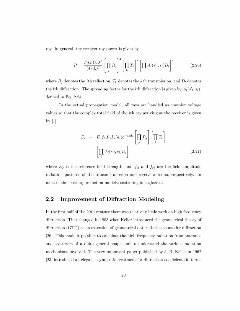
ray. In general, the receiver ray power is given by
Pi =PtGtGrλ
2
(4πdi)2
∏j
Rj
2 [∏k
Tk
]2 [∏l
Al(s′l, sl)Dl
]2
(2.26)
where Rj denotes the jth reflection, Tk denotes the kth transmission, and Dl denotes
the lth diffraction. The spreading factor for the lth diffraction is given by Al(s′l, sl),
defined in Eq. 2.24.
In the actual propagation model, all rays are handled as complex voltage
values so that the complex total field of the ith ray arriving at the receiver is given
by [1]
Ei = E0ftifriLi(di)e−jkdi
∏j
Rj
[∏k
Tk
][∏
l
Al(s′l, sl)Dl
](2.27)
where E0 is the reference field strength, and fti and fri are the field amplitude
radiation patterns of the transmit antenna and receive antenna, respectively. In
most of the existing prediction models, scattering is neglected.
2.2 Improvement of Diffraction Modeling
In the first half of the 20th century there was relatively little work on high frequency
diffraction. That changed in 1953 when Keller introduced the geometrical theory of
diffraction (GTD) as an extension of geometrical optics that accounts for diffraction
[26]. This made it possible to calculate the high frequency radiation from antennas
and scatterers of a quite general shape and to understand the various radiation
mechanisms involved. The very important paper published by J. B. Keller in 1962
[23] introduced an elegant asymptotic treatment for diffraction coefficients in terms
20

of certain canonical problems that include fields diffracted by straight edges, curved
edges, corners or tips, and surfaces. All the diffraction coefficients vanish as the
wavelength λ tends to zero.
However, the GTD failed in the vicinity of the shadow boundaries of the inci-
dent and reflected fields and consequently it was not suitable for general application
to radio propagation over diffracting edges. So the uniform GTD (UTD) was devel-
oped to overcome this limitation. In the UTD, the canonical problems are solved
by uniform asymptotic methods [24], and the resulting diffracted field not only de-
scribes the field in the shadow region, but also compensates for the discontinuities
in the geometrical optics field at the shadow boundaries.
Luebbers [25] modified the diffraction coefficient developed by Kouyoumjian
and Pathak in [24] to include finite conductivity and local surface roughness ef-
fects. By incorporating the Fresnel reflection coefficients in the diffraction coeffi-
cient, Luebbers’ heuristic method obtained significant improvement in accuracy for
geometries with grazing incidence in comparison to the Fresnel knife edge diffraction,
which neglected the shape and composition of diffracting surface.
Because the heuristic model proposed by Luebbers can be easily and effi-
ciently implemented in a computer program, this formulation is currently used in
many ray-tracing propagation predictions [1, 27–29]. However, this model intro-
duced an artificial dip (in the illuminated or shadow region) in the diffracted field
strength. In order to eliminate the physical inaccuracy of this model, Remley et
al. [30] proposed a new set of diffraction coefficients that the “effective” angles at
which the Fresnel coefficients were calculated were redefined based on whether the
angle of incidence was greater than or less than 180o, as explained subsequently, and
whether the observation point is in the illuminated region. The new diffraction coef-
ficient formulations ensured that the diffracted rays always decrease monotonically
away from the shadow boundaries.
21

The UTD is the uniform extension of the GTD since it has valid solutions
everywhere. However, the UTD still suffers from some of the deficiencies of the
GTD; namely, the theory fails when the incident field is not a ray-optical field,
and it cannot be applied when the reflection and diffraction are no longer local
phenomena. Researchers have developed formulations to compensate for the above
mentioned shortcomings. Slope diffraction is used in cases where the incident field
has a rapid spatial variation, e.g., in the edge-transition regions.
Wedge diffraction formulations and the application of diffraction theory to
propagation prediction modeling have been studied and improved by many re-
searchers. This section intends to give a thorough study of various mathematic
constructions originating from the geometric theory of diffraction (GTD), which in-
clude the uniform theory of diffraction (UTD), heuristic expression of diffraction
coefficient, slope diffraction, and other methods.
2.2.1 GTD Diffraction Coefficient
Keller postulated that high-frequency diffracted rays would depend strongly on the
geometry in the immediate vicinity of the point of the diffraction. Analogous to
reflected fields in geometric optics (GO), diffracted fields can be expressed by the
incident field on the diffraction point multiplied by a diffraction coefficient, a spread-
ing factor, and a phase term. In general, the diffracted field Ed at a distance s from
the diffraction point has the form
Ed(s) = EiDA(s)e−jks (2.28)
where Ei is the field incident at the point of diffraction on the edge, D is the
diffraction coefficient, and A(s) is the spreading factor defined by Eq. 2.24.
By comparing the solution for the diffracted field in (2.28) to an asymptotic
expansion of Sommerfeld’s solution to Helmholtz equation [23], Keller found that
22
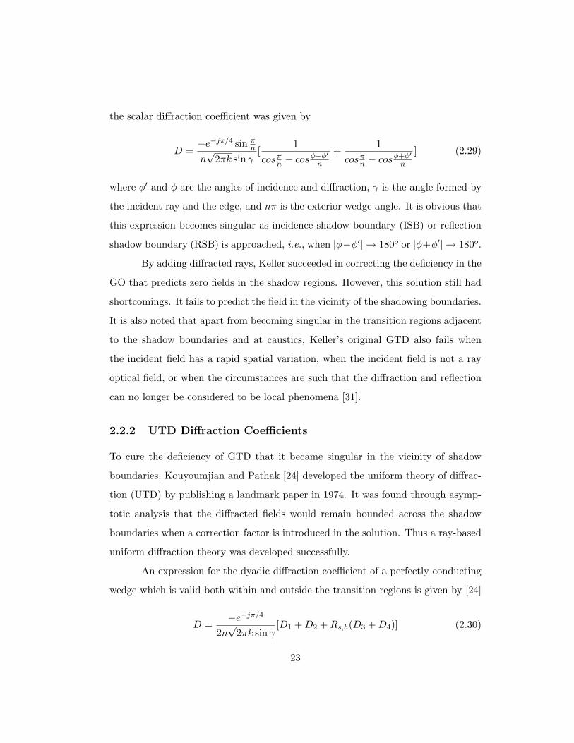
the scalar diffraction coefficient was given by
D =−e−jπ/4 sin π
n
n√
2πk sin γ[
1cosπ
n − cosφ−φ′
n
+1
cosπn − cosφ+φ′
n
] (2.29)
where φ′ and φ are the angles of incidence and diffraction, γ is the angle formed by
the incident ray and the edge, and nπ is the exterior wedge angle. It is obvious that
this expression becomes singular as incidence shadow boundary (ISB) or reflection
shadow boundary (RSB) is approached, i.e., when |φ−φ′| → 180o or |φ+φ′| → 180o.
By adding diffracted rays, Keller succeeded in correcting the deficiency in the
GO that predicts zero fields in the shadow regions. However, this solution still had
shortcomings. It fails to predict the field in the vicinity of the shadowing boundaries.
It is also noted that apart from becoming singular in the transition regions adjacent
to the shadow boundaries and at caustics, Keller’s original GTD also fails when
the incident field has a rapid spatial variation, when the incident field is not a ray
optical field, or when the circumstances are such that the diffraction and reflection
can no longer be considered to be local phenomena [31].
2.2.2 UTD Diffraction Coefficients
To cure the deficiency of GTD that it became singular in the vicinity of shadow
boundaries, Kouyoumjian and Pathak [24] developed the uniform theory of diffrac-
tion (UTD) by publishing a landmark paper in 1974. It was found through asymp-
totic analysis that the diffracted fields would remain bounded across the shadow
boundaries when a correction factor is introduced in the solution. Thus a ray-based
uniform diffraction theory was developed successfully.
An expression for the dyadic diffraction coefficient of a perfectly conducting
wedge which is valid both within and outside the transition regions is given by [24]
D =−e−jπ/4
2n√
2πk sin γ[D1 + D2 + Rs,h(D3 + D4)] (2.30)
23

where γ is the angle formed by the incident ray and the edge, and Rs,h are the soft
and hard reflection coefficients of the wedge edge corresponding to Dirichlet and
Neumann boundary conditions
Ez = 0 (2.31)
or∂Hz
∂n= 0 (2.32)
respectively. For a perfectly conducting edge, Rs,h = ∓1. The components of the
diffraction coefficients in (2.30) are given by
D1 = cotπ + (φ− φ
′)
2nF (kLa+(φ− φ
′)) (2.33)
D2 = cotπ − (φ− φ
′)
2nF (kLa−(φ− φ
′)) (2.34)
D3 = cot(π − (φ + φ
′)
2n)F (kLa−(φ + φ
′)) (2.35)
D4 = cot(π + (φ + φ
′)
2n)F (kLa+(φ + φ
′)) (2.36)
and
F (x) = 2j√
xejx∫ ∞
√x
e−jτ2dτ (2.37)
is the transition function,
L =ss′
s + s′sin2γ (2.38)
a+(β) = 2cos2(2nπN+ − β
2) (2.39)
a−(β) = 2cos2(2nπN− − β
2) (2.40)
where
β = φ + φ′ or β = φ− φ′ (2.41)
24

Figure 2.3: Transition function F (X).
The parameters s, s′, φ, and φ′ are specified as in Fig. 2.2.
In the above equations, N+ and N− are integers that most nearly satisfy the
equations
2πnN+ − β = π (2.42)
2πnN− − β = −π (2.43)
The transition function F (X) defined in the preceding expression involves a
Fresnel integral. Fig. 2.3 shows the magnitude and phase of F (X), where X = kLa.
2.2.3 Luebbers’ Heuristic Model
Luebbers [25] introduced a heuristic modification to the UTD equations in Kouy-
oumjian and Pathak’s solution. Fresnel reflection coefficients corresponding to the
dielectric material of the diffracting wedge are incorporated into the UTD coefficient
25

terms associated with the RSB. Hence the diffraction coefficient becomes
D =−e−jπ/4
2n√
2πk sin γ[D1 + D2 + R0D3 + RnD4] (2.44)
where Di’s are defined as in the section 2.2.2. R0 and Rn are the Fresnel reflection
coefficients defined by Eq. 2.11 for the 0 face and for the n face respectively. The
angle in Eq. 2.11 is the incidence angle φ′ for R0, and the diffraction angle nπ − φ
for Rn. A comparison of rigorous and heuristic solutions is available in [32].
2.2.4 Regional Modification
As discussed by Luebbers, the accurate use of these heuristic diffraction coefficients
is restricted to applications meeting certain conditions: The obstacles (wedges) must
have large interior angles, the observation points must be near shadow boundaries,
and the observation angles must be greater than the angles of incidence. In cases
where these conditions are not satisfied, a nonphysical dip in the diffracted field
may result for certain angles of observation. Remley et al. [30] refined the angular
dependence of the diffraction coefficients in a more physical way.
In Luebbers’ formulation, the Fresnel reflection coefficients R0 and Rn are
calculated at the angles of θ0 = φ′ and θn = nπ − φ, respectively. It is noticed that
only the observation point, in terms of φ, determines Rn for a fixed wedge. Since
RSB depends on the angle of incidence φ′, Rn should be determined by both the
angle of incidence φ′ and the angle of diffraction φ. Two factors are involved in
the new formulation: whether the angle of incidence is greater than or less than
180o (measured from the zero face), and whether the observation point φ is in the
illuminated region, i.e., |φ − φ′| < 180o, or in the shadow region. Table 2.2 lists θ0
and θn for four different cases proposed in [30].
26

Region θ0 θn
φ′ < π, illum. −φ′ −(φ + φ′)φ′ < π, shadow φ′ nπ − (φ + φ′)φ′ > π, illum. φ′ nπ − (φ + φ′)
φ′ > π, shadow. nπ − φ′ φ
Table 2.2: Angles Involved in the calculation of diffraction coefficient
2.2.5 Comparison and Discussion
The received signals predicted by different mathematical constructions that are de-
scribed in the previous sections are plotted in Figure 2.4. Keller’s expression for
a perfectly conducting wedge results in discontinuity at the RSB and ISB bound-
aries. Kouyoumjian and Pathak fixed this problem. But their formulation does
not consider the material of the wedge. A perfectly conducting wedge is assumed
and consequently the error in the shadow region is big. It is shown that Lueb-
bers’ construction gives significant improvement for the cases of grazing diffraction
angles. However, it inevitably leads to a nonphysical dip when the angle of diffrac-
tion is small. With Remley et al.’s formulation, the diffracted rays always decrease
smoothly and monotonically away from the shadow boundaries.
2.2.6 Multi-Edge Transition Zone Diffraction
When the incident field is not ray-optical, for instance, in the case of double-wedge
diffraction, conventional UTD is not sufficient because the second wedge is illumi-
nated by a transition-region field. In a region involving no more than one transition
region, slope diffraction yields good results [33]. Holm [33] considered perfectly
absorbing and conducting knife edges and noncurved wedges by expanding the inte-
gral of Vogler’s solution [34] to find higher order diffracted fields in a UTD context.
However the diffraction process involves excessive computations for high order terms
which is not practically feasible. J. B. Andersen [35] applied slope diffraction to mul-
27

Figure 2.4: Comparison of different formulations of the diffraction coefficient forwedges (φ′ = 22o, s′ = 28.0 m, s = 27.5 m, f = 900 MHz, σ = 0.1 S/m, εr = 15.0).
tiple absorbing screens in the transition zones of the shadow boundaries, which is
a first-order effect in transition zone diffraction. The solution was ensured to have
continuity of amplitude and slope at each point.
Slope Diffraction
The total edge-diffracted field consists not only of the first-order diffracted field,
but also of the so-called slope-diffracted fields. Whereas the first-order diffracted
field is proportional to the amplitude of the incident field at the diffraction point,
the slope-diffracted field is proportional to the derivative of the incident field at the
diffraction point. When a source is reasonably close to the edge, the slope-diffracted
field can be quite substantial. With slope diffraction involved, the total diffracted
field will then become
E =[EiD(α) +
∂Ei
∂nds(α)
]A(s)e−jks (2.45)
28

where α ≡ φ − φ′, D(α) is the amplitude diffraction coefficient, and ds(α) is the
slope diffraction coefficient denoted as
D(α) = − e−jπ/4
2√
2πkcos(α/2)F (2kLcos2(α/2)) (2.46)
ds(α) =1jk
∂D(α)∂α
(2.47)
As the derivative of the transition function F (x) is
F ′(x) = j[F (x)− 1] +F (x)2x
(2.48)
and accordingly
ds(α) = −e−jπ/4
√2πk
Ls sin(α/2)[1− F (x)] (2.49)
It should be noted that ∂Ei/∂n is the directional derivative of the incident field in
the normal direction of the ISB, pointing from the shadow region to the lit region.
In the two-dimensional case ∂Ei/∂n can be formulated in cylindrical coordinates.
Because n = φs, we have
∂Ei
∂n=(
∂Ei
∂ρρ +
1ρ
∂Ei
∂φsφs +
∂Ei
∂zz
)· φs (2.50)
so that∂Ei
∂n=
1ρ
∂Ei
∂φs=
1s
∂Ei
∂φs(2.51)
as shown in Fig. 2.5.
The L and Ls parameters, in Eq. 2.46 and 2.49 respectively, are calculated
to ensure continuity of the diffracted field and its slope along the shadow boundaries
of the edges. So the incident wave on the second edge consists of two components,
an amplitude wave and a slope wave, where the amplitude wave is the combined
incident and amplitude diffracted wave.
29

Figure 2.5: Directional derivative
Figure 2.6: Multiple-edge transition zone diffraction
Multiple Knife-Edge Diffraction
Consider the case of transition zone diffraction shown in Fig. 2.6, where α is the
angle from the ISB to the line connecting the edge and the observation point. When
α is large, x is large in (2.48), indicating rays in the normal diffraction region
characterized by GTD. We are interested in the case when α is small, i.e., in the
vicinity of the ISB - the transition region.
Andersen specified some general principles for computing multiple-edge diffrac-
tions [36]:
• At each edge, the incident field is diffracted with an amplitude diffraction
30

coefficient of D,
• At each edge, the incident slopes are diffracted with different slope diffraction
coefficient ds,
• Since the slopes are different for the various constituents depending on their
origin, we must keep track of the slopes originating from each edge.
Tzaras and Saunders [37] improved the heuristic UTD solution by Andersen
[35]. The innovation in the approach by Tzaras and Saunders is to develop different
continuity equations which vary for each ray independently so that D(α) and ds(α)
vary with diffracted rays. Their method, with a little added complexity, provides
more accurate output than Andersen’s because both the magnitude and the phase of
the signal are involved in enforcing amplitude and slope continuity over the shadow
boundary for the calculation of the L and Ls parameters. Hence, the field incident
on edge m is given by
Em =m−2∑n=0
Enm +[Em−1Dm−1(α) +
∂Em−1
∂ndm−1(α)
]Am−1(sm−1)e−jksm−1 (2.52)
where the first summation term is the total field at edge m with edge m− 1 absent,
resulting in an (m − 2)-edge diffraction problem. The terms in the square bracket
are analyzed for all the components of the field at edge m− 1 since the diffraction
coefficient could possess different values for different rays. It is seen that the field at
a given point after N edges needs information from all previous edges for that point.
Thus transition zone diffraction has “memory” in contrast to the GTD multiplication
of independent factors. This is indeed the cost in computation to apply ray theory
in transition regions. Fast computation can still be achieved by implementing the
computer algorithm recursively.
31

2.3 Diffraction in Propagation Prediction
In this section, existing UTD-based models are reviewed with a focus on determin-
istic propagation estimation in microcellular urban environments. New challenges
to the diffraction theory as well as its application to modeling are described. Ap-
proaches to increase the accuracy and efficiency of site-specific modeling methods
are presented for future exploration.
2.3.1 Importance of Diffraction in Propagation Prediction
Accurate characterization of wave propagation is essential to successful system de-
ployment and network planning. Current channel estimations provide two types
of parameters, the large-scale path-loss coverage information and small-scale fading
statistics for equalization, coding, and transceiver design [38]. The effect of diffrac-
tion in site-specific modeling is important for accurate signal estimation when a LOS
path does not exist. For instance, in a microcellular urban environment, diffractions
from vertical and horizontal edges of buildings make important contributions to the
received power. When the LOS path is not present from the transmitter to the
receiver, the diffracted field makes the dominant contribution to the received sig-
nal power. According to the asymptotic evaluation, only extremely high frequency
tends to have negligible diffracted fields. Since the frequencies of the signals used in
current wireless applications such as WLAN are still below 10 GHz, it is important
to take diffracted fields into consideration. Especially in the cases when diffracted
fields are dominant, incomplete account of various rays will significantly degrade
the ray-tracing accuracy. Therefore, the application of diffraction theory within the
scope of UTD in propagation modeling has been an important research topic in the
past decade.
32

2.3.2 UTD Propagation Models for Microcellular Communications
Several prediction models based on ray optics and diffraction theory have been
reported in the literature [2, 28, 32, 39–42]. However, most of these models are
restricted to path loss prediction. For city street and indoor single floor scenes, only
very few models have been published for comparisons of power delay profiles on
a location-by-location bases to assess the applicability of the model for predicting
wideband characteristics, i.e., individual multipath components in terms of their
time delays [1, 43].
Narrowband prediction
Many researchers have adopted the UTD diffraction coefficient to predict the diffracted
field in city street junction scenarios [2,28,32,40–42], and in corridors of office build-
ings [44]. Most of them employed Luebbers heuristic formulation and some presented
new heuristic models to simplify the calculation in the prediction procedure.
For instance, Tan and Tan developed a microcellular communications prop-
agation model based on the UTD and multiple image theory for microcells in Tokyo
and New York [2, 39], and Ottawa [45]. The model includes contributions to the
received signal from all possible propagation paths, including ground and wall re-
flections from diffracted and specularly reflected signals both in the LOS and out-of-
sight (OOS) regions. The tall building walls are treated as flat surfaces with average
relative permittivity and conductivity and the buildings at street corners are mod-
eled as conducting wedges which inevitably limited the accuracy of the model.
Wideband prediction
Seidel and Rappaport [1] developed a three-dimensional ray-tracing algorithm and
validated the prediction results with measurements in various buildings on the cam-
pus of Virginia Tech. Luebbers heuristic formulation was adopted in their method
33
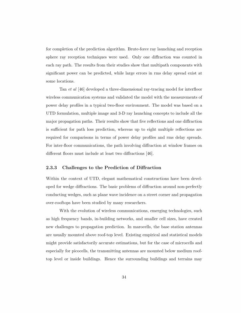
for completion of the prediction algorithm. Brute-force ray launching and reception
sphere ray reception techniques were used. Only one diffraction was counted in
each ray path. The results from their studies show that multipath components with
significant power can be predicted, while large errors in rms delay spread exist at
some locations.
Tan et al [46] developed a three-dimensional ray-tracing model for interfloor
wireless communication systems and validated the model with the measurements of
power delay profiles in a typical two-floor environment. The model was based on a
UTD formulation, multiple image and 3-D ray launching concepts to include all the
major propagation paths. Their results show that five reflections and one diffraction
is sufficient for path loss prediction, whereas up to eight multiple reflections are
required for comparisons in terms of power delay profiles and rms delay spreads.
For inter-floor communications, the path involving diffraction at window frames on
different floors must include at least two diffractions [46].
2.3.3 Challenges to the Prediction of Diffraction
Within the context of UTD, elegant mathematical constructions have been devel-
oped for wedge diffractions. The basic problems of diffraction around non-perfectly
conducting wedges, such as plane wave incidence on a street corner and propagation
over-rooftops have been studied by many researchers.
With the evolution of wireless communications, emerging technologies, such
as high frequency bands, in-building networks, and smaller cell sizes, have created
new challenges to propagation prediction. In marocells, the base station antennas
are usually mounted above roof-top level. Existing empirical and statistical models
might provide satisfactorily accurate estimations, but for the case of microcells and
especially for picocells, the transmitting antennas are mounted below medium roof-
top level or inside buildings. Hence the surrounding buildings and terrains may
34

create wide shadow regions. The received signals result from a combination of all
possible reflections from walls and ground surfaces, diffractions from building edges,
and scattering from rough surfaces. Various deterministic and empirical models have
been developed based on the dominant physical phenomena and the specification of
the environmental data.
To deal with the complex indoor propagation environments in which WLAN
is deployed, appropriate prediction of diffraction becomes vital for accurate overall
propagation prediction. To meet these challenges, existing prediction methods need
to be modified and improved, and new procedures and techniques have to be devel-
oped. This thesis in Chapter 4 offers promising, novel techniques that have been
validated by measurement.
2.4 Summary
Appropriate modeling of the radio environment must include free space propaga-
tion, specular reflection, transmission, diffraction, and scattering. Researchers have
developed various heuristic constructions of the diffraction coefficient in the scope
of UTD to improve propagation modeling for microcellular communication systems.
Adequate prediction of wideband characteristics, however, still needs more improve-
ment, and faster computational techniques are needed.
35

Chapter 3
Ray-Tracing Based Site-Specific
Modeling
3.1 Introduction
With the input of environmental data, ray-tracing models provide accurate site-
specific means to obtain useful simulation results for coverage prediction and mul-
tipath fading characterization. According to the ray optics and the uniform theory
of diffraction (UTD), propagation mechanisms may include direct (LOS), reflected,
transmitted, diffracted, scattered, and some combined rays, which, in fact, compli-
cates the calculation procedure. Hence many researchers have proposed improve-
ment methods to make the ray-tracing procedure more efficient. In this section, the
basic models of ray-tracing methods are briefly described.
3.1.1 Brute-Force Ray Launching Algorithm
The basic procedure of the brute-force method [47] is to exhaustively search in all
directions from the transmitter to trace all possible ray paths. When an object is
hit by incident rays, reflection, transmission, diffraction, or scattering will occur,
36

Figure 3.1: A schematic illustration of the brute-force method.
depending on the geometry and the electric properties of the object. When a ray
is received by a receiving antenna, the electric field (or power) associated with the
ray is calculated. A schematic illustration of the brute-force method is shown in
Fig. 3.1. The radiation sphere around the transmitter is divided into solid angular
segments from which rays are launched.
When launching a ray, it is either treated as a ray tube or a ray cone. When
ray cones are used to cover the spherical wavefront at the receiving location, these
cones have to overlap. For the ray-cone scheme, the reception test can be carried
out by using a reception sphere centered at the receiving point with radius equal to
αd/√
3 [1], where α is the angle between two adjacent rays and d is the unfolded
length of the ray path. Since ray cones are overlapped, ray double counting will occur
when a receiving point is located in the overlapping area between the ray cones. To
avoid errors, some procedures have been proposed to deal with this issue [48].
3.1.2 Image Method
The image method is a simple and accurate method for determining the ray tra-
jectory between the transmitter(Tx) and receiver(Rx). The basic idea of the image
method is shown in Fig. 3.2. For this simple case, the image of Tx due to W1
is first determined (Tx1). Then the image of Tx1 due to W2 is calculated (Tx2).
37

Figure 3.2: A schematic illustration of the image method.
The reflection point (P2) on W2 can be found by connecting Rx and Tx2 while the
reflection point (P1) on W1 is the intersection point of the line connecting P2 and
Tx1 with the reflecting plane W1. Imaging theory replaces reflecting walls and cor-
ners with images of the illuminating source [49,50]. The image method is accurate,
but can be cumbersome, suffering from inefficiency when large numbers of reflecting
surfaces are encountered and the intersection testing times are high. For realistic
applications, special techniques have to be adopted to reduce the computation time.
3.1.3 Hybrid Methods
To expedite the ray-tracing procedure, some hybrid methods that combine the image
and brute-force methods have been used [1, 2]. In those methods, the brute-force
method is first used to quickly identify a possible ray path from Tx to Rx. The
exact intersection points can then be accurately found with the image method. The
basic idea of the hybrid methods is to explore the advantages of both brute-force
38

(efficient) and image (accurate) ray-tracing methods.
One of the primary computation tasks in the ray-tracing algorithms is to
determine the dominant ray propagation paths, i.e., to determine the rays that
affect the received signal significantly. The efficient calculation of dominant ray
propagation paths for ray-tracing models has been an active area of current research.
3.2 Acceleration of Ray-Tracing Algorithms
Due to the simplicity of the ray-tracing method, it is widely used in the area of
site-specific propagation prediction and consequently many researchers focused on
tackling the problem of computational inefficiency of the ray-tracing algorithms.
One way to achieve efficiency is to reduce the number of intersection tests on the
ray paths, and the other is to accelerate the intersection test procedure. All acceler-
ation methods take into account the preprocessing of the propagation environments
and/or the positions of Tx and/or Rx.
3.2.1 Angular Z-Buffer (AZB)
The AZB method is based on the light buffer technique used in computer graphics
[51, 52]. The basic idea is to divide the space into angular regions according to a
source point which can be a Tx or an image of it with respect to a reflection plane.
When a ray is launched from the source point, only objects located in the angular
region containing the ray will be tested for ray intersection. The disadvantage of this
method lies in that when multiple reflections are involved, there are many source
points and an AZB needs to be established for each of them, which is not easy for
preprocessing.
39

3.2.2 Ray-Path Search Algorithm
Based on the idea that ray-tracing routines should be applied only to those areas
where rays are likely to exist, a visibility graph is employed in the ray-path search
algorithms [53,54] to limit the intersection test. The visibility graph contains several
layers. The first layer includes all objects visible to the Tx (for LOS rays). The
second layer contains objects visible to the first layer (for transmitted, reflected, and
diffracted rays). Further layers are of similar recursive relationship. Since it is not
easy to determine the visibility between two objects, bounding box is sometimes
employed in establishing the visibility graph.
When a ray is launched from the Tx, only those objects in the first layer of
the visibility graph need to be tested for the first intersection. To determine the nth
intersection of a ray in a path, only objects in the nth layer need to be tested, thus
leading to saving of computation time.
The visibility graph method has similar drawbacks to the AZB method in
the sense that when interaction levels are high, the establishment of the visibility
graph will be much more time consuming and complicated.
3.2.3 Dimension Reduction Method
To achieve efficient ray-tracing procedures and retain acceptable accuracy, ray-
tracing algorithms may be carried out in non full 3-D geometries. Examples of this
approach may include the 2-D/2.5-D method, the vertical plane launch method,
etc., as explained.
2-D/2.5-D Method
In a microcellular environment, particularly when the buildings in a region are
much taller than the Tx, the complex 3-D environment can be approximated by
much simpler 2-D structures (where the buildings are assumed to be infinitely tall)
40

and the computational intensity of the ray-tracing procedure will be significantly
reduced [28].
Vertical-Plane-Launch (VPL) Method
The VPL technique is proposed in [55]. The usual 2-D ray tracing is used in a
horizontal plane. Each ray in the 2-D case represents a vertical propagation plane.
When a ray hits a vertical wall, specular reflection from the vertical wall and diffrac-
tion from the rooftop horizontal edge can occur. When the ray hits a vertical edge,
diffraction also occurs. The over-rooftop diffraction creates two vertical propagation
planes, one in the same direction as the incident ray and the other in the direction
of reflection. Diffraction from the vertical edge creates a new source and many new
rays in 2-D planes should be launched. These rays are further traced in a similar
manner until some criteria are reached.
Rizk et al. [56] compared the results using lateral, full 3-D, and VPL methods.
It is found that when the average building heights are around the Tx height, VPL
can give very good predictions.
3.2.4 Space-Division Method
The space-division method is widely used in computer graphics. The basic idea is
to first create a grid (usually rectangular) in the propagation environment, and then
establish a lookup table registering objects residing in each grid cell. When a ray
is launched, it is traced in the grid. For each grid the ray is traversing, the lookup
table is checked to see if any objects reside in the grid. If yes, the ray is tested for
intersection with these objects. If any object is hit, a reflected (or diffracted) and/or
a transmitted ray will be created and the new rays will be further traced.
The space-division method can give fast ray traversing and efficient ray trac-
ing. This is due to the fact that the algorithm for traversing the grid can be fast
41

and the intersection test is performed only on a small number of objects.
Rectangular Division
The most widely used space-decomposition method is the rectangular method. A
unique ray-tracing method was developed by Yun et al. [57] employing fast ray-
traversing algorithm over a rectangular grid. It requires that the wall should be
exactly located on the grid lines to obtain best efficiency.
Triangular Division
Triangular division is also very popular and is supported by many commercial soft-
ware such as SGI OpenGL. In 2D cases, a triangular mesh is used to discretise the
propagation region of interest. In 3D cases, tetrahedral or triangular cylinders may
be used [58].
3.3 Improvement of Accuracy of Ray-Tracing Algorithms
Due to the fact that the environmental data input to a ray-tracing engine may not
be accurate and all of the materials of the objects in the region of interests may not
be known, the ray-tracing method can only provide approximate results for realistic
propagation environments [38]. Another factor that affects the accuracy of the ray-
tracing procedure is the incomplete accounts of all kinds of rays because taking more
rays into account inevitably increases the computation intensity.
Diffractions from wall edges are important contributions to the received
power, particularly for the non-LOS (NLOS) case. Methods for calculation of
diffraction coefficients for metal or materials with finite conductivity were devel-
oped in [24, 25, 59]. A comparison among the perfectly absorbing wedge (PAW)
method, UTD, and UTD heuristic methods is provided in [28]. It is found that
errors given by these three methods are comparable.
42

3.4 Site-Specific Statistical Modeling
Ray-tracing algorithms have been used for accurate prediction in site-specific prop-
agation modeling in spite of its computational intensity. Statistical models, on the
other hand, offers computational simplicity but poorer accuracy. In order to achieve
computational efficiency, Hassan-Ali and Pahlavan [60] proposed a new model for
predicting indoor radio propagation. This new model is based on the statistical
derivation of the ray-tracing operation. The patterns and lengths of rays in differ-
ent paths between the transmitter and receiver are related to statistical parameters
of the site-specific features of indoor environment, such as the floor plan geometry.
In this model, three site-specific parameters, which are mean free distance, mean
transmission coefficient, and mean reflection coefficient, are directly related to the
geometry of the floor layout, the materials of walls, door, and windows. By geo-
metric optics and geometric probability, a simple equation for power delay profile is
derived as follows.
When a ray arrives at the receiver, it has already gone through many re-
flections and transmissions (object intersections). Each time an object-intersection
occurs, the ray loses a certain amount of power while the propagation loss between
intersections will maintain the free-space inverse-square distance law. Only reflec-
tions and transmissions are taken into account.
After traveling a path distance l and undergoing n intersections, including
m reflections and (n−m) transmissions, the mean path power, is expresses as
P (l) = Pol−2
∞∑n=0
n∑m=0
f(n, m|l)R2mT 2(n−m) (3.1)
where R and T are the mean “voltage” reflection and transmission coefficients,
respectively, and Po is the free-space power at distance 1 meter. The PDF of a path
that intersects n objects after travelling distance l with m reflections and (n −m)
43

transmissions, f(n, m|l), is further decomposed into the product of two PDFs that
characterize the n intersections and m reflections respectively, i.e.
f(n, m|l) = f1(n|l)f2(m|n, l) (3.2)
By Monte Carlo simulations, the probability of n intersections after travelling dis-
tance l is a Poisson distribution for the indoor environment. Hence
f1(n|l) =(λl)n
n!e−λl (3.3)
where 1/λ is the mean free distance between two intersections depends on the floor
layout.
The probability of having m reflections and (n − m) in path length l is a
binomial distribution
f2(m|n, l) =
n
m
pm(l)qn−m(l) (3.4)
where p(l) and q(l) are the probabilities of reflection and transmission, respectively,
for a path of length l. Obviously p(l) + q(l) = 1. p(l) and q(l) are determined as a
function of the difference between the total path length l and the LOS distance L
by assuming that the reflection and transmission events take place equally likely.
Through a few manipulations, the mean path power becomes
p(l) = Pol−2e−λleλl(qT 2+pR2) (3.5)
This equation gives an explicit relationship between the average power of a path
with site-specific details and the building layout via λ, and the floor materials via
R and T .
44

The mean reflection and transmission coefficients are the mean of various
corresponding coefficients for all objects enclosed in an area of ellipsoid shape, whose
foci are the locations of Tx and Rx and boundary acts as the farthest reflector on
which rays bounce with the same length. Then R and T are estimated as
R =∑k
i=1 SiRi∑kk=1 Si
(3.6)
T =∑k
i=1 SiTi∑kk=1 Si
(3.7)
where Ri, Ti, and Si are reflection, transmission, and size coefficients, respectively,
for object i. In the two dimensional case, Si is the length of the object. The
reflection and transmission coefficient Ri and Ti are defined as in Eq. 2.11 and χ is
a coefficient that accounts for the transmission loss and is usually taken to be 0.5.
The estimation of the mean value of a random variable λ uses the geometric
probability distributions of a ray within a rectangular shape as described in [60].
The multipath power at a wideband receiver is then defined as the sum of the powers
of individual paths:
P (L) =∫ ∞
l=LP (l)dl ∼=
∞∑i=0
P (L + iδ) (3.8)
where δ/c is the bin time unit, assuming that a path exists in each bin, which is 5
ns in this case.
This prediction is simpler than the ray-tracing method and possesses better
accuracy than statistical method. It has an error bound of 5 dB with respect to the
ray-tracing and measurement data. Hence this model can be accepted to surrogate
the use of the brute-force ray-tracing technique for prediction of radio propagation in
indoor environments. The method was validated in the UHF band at 900 MHz [60].
45

3.5 Site-Specific System Simulator for Wireless System
Design (S4W )
S4W , developed at Virginia Tech, is a parallel computing ray-tracer supported by
MPI (message passing interface). It calculates power delay profiles (PDPs) for a
given 3D polygonal environment. The complete package S4W is composed of a par-
allel ray tracer that provides an accurate assessment of propagation characteristics
for a given physical environment and a problem solving environment (PSE) suite
that support the inclusion of new models for predicting the performance of wireless
systems in specific environments.
3.5.1 Background of S4W
The ray-tracing algorithm employed in S4W was originated from Seidel and Rappa-
port’s early work in 1990s [1,61]. S4W uses pyramidal beams to model electromag-
netic waves. By tessellating the faces of an icosahedron and extrapolating points to
the surface of an encapsulating sphere, a geodesic dome is drawn and shooting beams
in all directions. Beams are traced through reflections and penetrations through ob-
structions in a particular environment. Once an intersection with a receiver location
is detected, a ray is traced back from the receiver location to the transmitter location
through the sequence of reflections and penetrations encountered by the beam [1].
With the collaboration between computer scientists and electrical engineers
at Virginia Tech, the first version of S4W (Site-Specific System Simulator for Wire-
less system design) became a testbed for academic research in novel computational
technologies [15,62].
S4W contains several improvements to the basic ray-tracing procedure in [1].
S4W uses octree space partitioning to reduce the number of intersection tests and
image parallelism with dynamic scheduling to reduce simulation runtime. As widely
46

used data structures in computer graphics and computer vision, octrees recursively
subdivide a 3D environment using cubes so that ray intersection computations can
be localized to a small set of elements. Image parallelism refers to the configura-
tion where each processor has a complete copy of the physical environment and is
appropriated with a fraction of the total number of rays to process. This has ad-
vantages over object parallelism in which each processor works with a partition of
the environment and the communication cost can be prohibitive [63].
The initial database interfacing in S4W1.0 requires many supporting tools
such as PostgreSQL relational database system, TCL/TK, EXPECT, etc. Although
these tools help to organize and manage a large set of scientific experiments, S4W1.0
was cumbersome for setup. More recently, an updated S4W1.01 was released. This
version provides an option to remove database interfacing and build a “LITE” ver-
sion that is more convenient for users who are solely interested in the simulation of
the radio signal propagation with a distributive ray-tracing engine.
Currently, S4W1.01 is being distributed as open-source software for academic
research. Through the Montage Project, a joint venture of UT-Austin and Virginia
Tech [16], S4W is being tested and enhanced actively at UT-Austin. First, the
diffraction effect in propagation has been incorporated in the software based on
a new efficient formulation of wedge diffraction [64, 65]. The newly enhanced S4W
has been used for propagation prediction in indoor office environment [66] and dense
urban area. The following sections describe the details.
3.5.2 S4W Ray-Tracer
The environmental data in terms of polygons is input in AutoCAD DXF format
and is converted into XML format. The space-division method adopted in S4W
is octree subdivision. In this method, a 3-D triangular grid is first built over the
propagation scene. Then the whole 3-D space is separated into eight boxes of equal
47

sizes, called octants or voxels (pixels with volume), by slicing the bounding box
with a horizontal plane and then a vertical plane. Based on the content in each
octree block, more subdivisions will be carried out in some/all of the child blocks.
In this way, a rooted tree is constructed and the leaves of the octree are the points
where the decomposition ends. The objective is to place the triangles that define
the scene in the nodes of the octree so that when a ray is tested for intersections
within a voxel, only the triangles in the corresponding octree leaf and its ancestors
are considered. Ideally, no intersection test is performed with the triangles that are
outside of the voxel, which is impossible in reality. The algorithm has to reduce the
number of useless intersection tests as much as possible.
Figure 3.3: An illustration example of S4W . (a) Input polygonal propagation envi-ronment. (b) Output (untrimmed) power delay profile at the receiver.
When a hierarchical spatial data structure is constructed to represent the
three dimensional volumetric data at different levels of details, the subsequent trac-
ing process is accomplished by an exhaustive search of all possible interactions with
the triangles. First, the ray-tracer determines if an LOS path exists between the
transmitter and the receiver. If the LOS path exists, the received field is computed.
48

Next, the program traces a source ray in a predefined direction to detect if an object
intersection occurs. If no intersection occurs, the process stops and a new source
ray is initiated. On the other hand, if an intersection has been found, the program
checks to see if a specularly reflected or transmitted ray has an unobstructed path to
the receiving location. After checking for reception, the program divides the source
ray into a transmitted and reflected ray that are initiated at the intersection point.
The reflected and transmitted rays are then treated separately in a similar fashion
as a source ray. This type of recursion continues until a maximum number of tree
levels is exceeded, the ray intensity falls below a specified threshold, or no further
intersections occur. Once an intersection with a receiver location is detected, a ray
is traced back from the receiver location to the transmitter location through the
sequence of reflections and penetrations encountered in the aforementioned tracing
procedure. Fig. 3.3 gives an example of the input and output of S4W . It is noted
that the diffraction, important in propagation especially around building edges and
corners, is neglected in the current released version S4W1.01 [67] because diffraction
modeling is computationally expensive.
3.6 Summary
In this chapter, the basic ray-tracing models and various existing methods that ac-
celerate and/or improve the accuracy of ray-tracing calculations have been reviewed.
Basically there are several ways to improve the ray-tracing based propagation pre-
diction models. One way is to accelerate the ray-tracing engines which mainly is
done in the preprocessing stage. Various computer graphics techniques need to be
explored. The second approach is to construct better physical models for prop-
agation mechanisms so that the new models are more appropriate for predictive
implementation. The third approach is to combine deterministic and stochastic
techniques to create some hybrid methods to expedite the prediction procedure. A
49

state-of-the-art ray-tracer, S4W , uses the parallel processing ray-tracing procedure
that employs triangulation and octree space division and modeling approaches. We
now use the S4W software infrastructure in the following studies that improve both
S4W and the state of the art in propagation predictions.
50

Chapter 4
Parametric Formulation of
Diffraction Coefficient for S4W
4.1 Introduction
As discussed in earlier chapters, real-time site-specific computation will be impor-
tant for future broadband devices that are able to use real-time processing to make
instant and proper wireless decisions [6]. As an important propagation mechanism,
diffraction must also be considered in existing wireless propagation prediction al-
gorithms for modeling the scattering phenomena particularly due to the presence
of building corners [1, 2, 40, 42]. Accordingly, effective and rapid evaluation of the
diffracted field also plays an important role in successfully characterizing large-scale
path loss in existing prediction tools, such as S4W .
Ever since the pioneering introduction of the UTD formulation for per-
fectly conducting wedges by Kouyoumjian and Pathak [24], many researchers have
proposed various wedge diffraction solutions for nonperfectly conducting surfaces,
which can be categorized as rigorous solutions [33, 68–72] and heuristic expres-
sions [25, 42, 73–76]. Most of the exact solutions are based on Maliuzhinets’ deriva-
51

tion [77] and are computationally prohibitive for real-time propagation prediction.
Hence in the early development of propagation prediction models, diffracted rays
tended to be neglected for the purpose of simplicity. In fact, the original version of
S4W that existed prior to this thesis did not include diffraction. Heuristic formu-
lations of diffraction, modified from the UTD diffraction coefficient in [24], enables
efficient evaluation of diffracted field by dielectric wedges. Among them, perhaps
Luebbers’ heuristic diffraction coefficient [25] is the most commonly adopted in the
field of propagation prediction modeling. Although this method offers easy imple-
mentation, it does not yield accurate estimation of the diffracted field in the shadow
region, which is particularly prominent in building and campus environments.
In order to improve the estimation of wedge diffracted fields for ray-tracing
based modeling methods, this chapter exploits inverse problem theory to find a bet-
ter approximation of the diffraction coefficient for a dielectric wedge that may be
rapidly computed. It begins with the high frequency solution presented by Tiberio
et al. [68] (see Eq. 4.2). In general, each of the four terms contains a multiplying
factor that is practically difficult to evaluate and needs a reasonable approximation.
This approach is to first approximate each multiplying factor with a two-dimensional
polynomial of the incidence angle and diffraction angle, then apply the least square
method to find the optimal polynomial coefficients. The resultant approximations
of the multiplying factors lead to much simpler calculation than the original sinu-
soidal expression. The comparison of the parametric formulation of the diffraction
coefficient with both rigorous solution and other heuristic formulations shows that
this method is advantageous in the sense that it is simpler than rigorous solutions
and more accurate than heuristic methods. The obtained solution enables fast and
accurate estimation of diffracted field in propagation modeling.
This chapter is organized as follows. In section 4.2, the diffracted field for a
wedge with surface impedance is expressed in the context of UTD as in the original
52

formulation for perfectly conducting wedge and the multiplying factors that are to be
studied are also specified. Section 4.3 describes the least-square criterion used in the
inverse analysis. The numerical results are compared with other solutions and the
influence of the parameters is investigated in Section 4.4. Section 4.5 describes the
incorporation of this new formulation in S4W . Section 4.6 presents the results of the
application of the parametric formulation in numerical simulation for some indoor
environments in on-campus building. Section 4.7 summarizes the contribution of
this novel fast diffraction computation technique that could be used eventually in
real-time calculations and which has been implemented in a new version of S4W .
4.2 UTD Formulation of the Problem
The geometry for the two-dimensional wedge diffraction problem is illustrated in
Fig. 4.1. It is customary to label the two faces of a wedge, the 0-face and n-
face, respectively, and consider the incidence angle φ′ and diffraction angle φ to
be measured from the 0-face. The exterior wedge angle is denoted by nπ. The
total field, which is the sum of geometrical optic fields, two surface wave fields, and
a diffracted field, was presented in terms of an exact integral by Maliuzhinets [77].
Tiberio et al. [68] then specify the rigorous solution and an asymptotic expression for
the diffracted field. For simplicity, only the two-dimensional problem is considered
in this work, while it is easy to extend to the three-dimensions by incorporating an
incidence angle β0 as in [24].
When a wedge is illuminated by a plane wave, the high-frequency solution
for the diffracted field Ed is given by
Ed(s) = EiDe−jks
√s
(4.1)
where Ei is the field incident at the point of diffraction on the edge and D is the
53
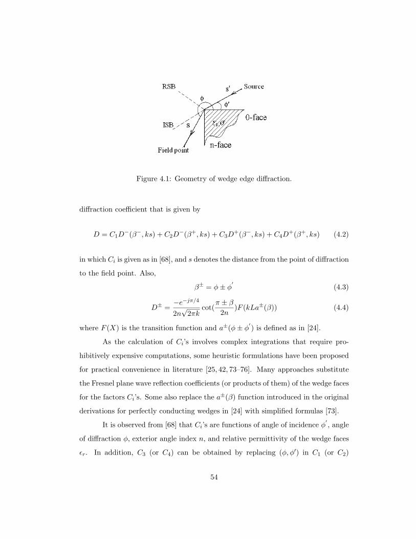
Figure 4.1: Geometry of wedge edge diffraction.
diffraction coefficient that is given by
D = C1D−(β−, ks) + C2D
−(β+, ks) + C3D+(β−, ks) + C4D
+(β+, ks) (4.2)
in which Ci is given as in [68], and s denotes the distance from the point of diffraction
to the field point. Also,
β± = φ± φ′
(4.3)
D± =−e−jπ/4
2n√
2πkcot(
π ± β
2n)F (kLa±(β)) (4.4)
where F (X) is the transition function and a±(φ± φ′) is defined as in [24].
As the calculation of Ci’s involves complex integrations that require pro-
hibitively expensive computations, some heuristic formulations have been proposed
for practical convenience in literature [25, 42, 73–76]. Many approaches substitute
the Fresnel plane wave reflection coefficients (or products of them) of the wedge faces
for the factors Ci’s. Some also replace the a±(β) function introduced in the original
derivations for perfectly conducting wedges in [24] with simplified formulas [73].
It is observed from [68] that Ci’s are functions of angle of incidence φ′, angle
of diffraction φ, exterior angle index n, and relative permittivity of the wedge faces
εr. In addition, C3 (or C4) can be obtained by replacing (φ, φ′) in C1 (or C2)
54

with (nπ − φ, nπ − φ′). Fig. 4.2(a) and 4.2(b) give an example of the curvature
surface of C1 and C3. As shown in the graphs, the factors C1 and C3 are complex
numbers. However, they have been taken as 1 for the purpose of simplification in
most heuristic formulations. The motivation is to use a polynomial curve fitting
approach to attempt to yield an easy, yet more accurate model to avoid the non-
physical artifacts that result from past heuristic approaches.
4.3 Inverse Solution of The Diffraction Coefficient
Each of the four terms in Eq. 4.2 corresponds to the situation when either surface is
shadowed (e.g. C1 and C3) or reflects the incident field (e.g. C2 and C4). Hence some
of the past approaches originated from the proper categorization of the illuminated
or shadow region. In contrast, the approach addresses the problem of diffraction
modeling using numerical analysis. From observation in [68], the multiplying factors
Ci’s are functions of sinusoids, where each sinusoid is essentially a summation of
polynomials. Further investigations reveal that the shapes of the curved surfaces
resemble hyperbolic sine and/or cosine. This indicates that appropriate polynomial
curve-fitting may yield good (if not optimal) approximations for the four multiplying
factors.
Assume that each surface is a product of polynomials P1(φ) and P2(φ′) of
degrees two or three. Then the least square criterion may be used to fit the curvature.
Since C1 and C3 are symmetric to each other, and so are C2 and C4, only C1 and C2
need to be considered for polynomial fitting. As shown in Fig. 4.2(a), we assume
that the surface of |C1|, denoted by S1(φ, φ′), is related to the diffraction angle φ
and the incidence angle φ′ in terms of P1(φ) and P2(φ′), i.e.,
S1(φ, φ′) = (a1φ2 + b1φ + c1)(a2φ
′2 + b2φ′ + c2) (4.5)
55

(a) |C1| and |C3|
(b) Phases of C1 and C3
(c) |C2| and |C4|
Figure 4.2: Surfaces of C1, C2, C3, and C4 (parallel polarization, εr = 6, σ =0.005 S/m, f = 900 MHz. The phases of C2 and C4 are approximately π and notshown in the graph.
56

Factor (a01, b
01, c
01(, d
01)) (a0
2, b02, c
02)
|C1| (0.057, -0.43, 1.82) (-0.0063, 0.030, 1.09)phase of C1 (0.014, -0.11, 0.13, 0.35) (-0.024, 0.11, 0.12)
|C2| (0.030, -0.22, 0.94) (0.09, -0.43, 1.08)
Table 4.1: Initial guesses for fitting C1 and C2
In order to find the optimal approximation S1(φ, φ′) to the surface S1(φ, φ′)
in the least square sense, an initial value of the coefficients (a01, b
01, c
01, a
02, b
02, c
02) is
obtained by two curve-fittings in the dimension of φ by setting φ′ = nπ/2 and in
another dimension of φ′ by setting φ = nπ/2, respectively (shown in Fig. 4.3(a) and
4.3(b)). The criterion for the inverse solution (shown in Fig. 4.4(a)) is defined such
that
(a1, b1, c1, a2, b2, c2) = arg min∑φ,φ′
(S1(φ, φ′)− S1(φ, φ′))2 (4.6)
For the case of fitting the phase surface of C1, two polynomials, P1(φ) =
a1φ3 + b1φ
2 + c1φ+ d1 of order 3 and P2(φ′) = a2φ′2 + b2φ
′+ c2 of order 2, are used.
The initial value (a01, b
01, c
01, d
01, a
02, b
02, c
02) is obtained by two one dimensional fittings
of P1(φ) at φ′ = nπ/2 and P2(φ′) at φ = nπ/2 (shown in Fig. 4.3(c) and 4.3(d)).
The inverse solution of the phase of C1 is shown in Fig. 4.4(b). The magnitude of
C2 is approximated using two second order polynomials, P1(φ) = a1φ2 + b1φ + c1
and P2(φ′) = a2φ′2 + b2φ
′ + c2. The initial value (a01, b
01, c
01, a
02, b
02, c
02) (as shown in
Fig. 4.3(e) and 4.3(f) ) is obtained in the same manner as for fitting the magnitude
of C1 and phase of C1. Fig. 4.4(c) shows the least-square optimized |C2| and the
exact solution computed in [68]. Since the phase of C2 takes values about π or −π,
it can be assumed to be π.
In summary, assuming that each magnitude or phase surface, denoted by
57

(a) |C1(φ, 135o)| (b) |C1(135o, φ′)|
(c) Phase of C1(φ, 135o) (d) Phase of C1(135o, φ′)
(e) |C2(φ, 135o)| (f) |C2(135o, φ′)|
Figure 4.3: Initial values of |C1|, phase of C1, and |C2|. The solid curves are therigorous solutions and the dotted curves are the initial guesses for the followingoptimizations. The numerical values are listed in Table 4.1.
58

Si(φ, φ′), is a product of two polynomials:
Si(φ, φ′) = [M∑
m=0
amφm][N∑
n=0
bnφ′n] (4.7)
where M,N = 2 or 3 depending on the shape of the surface. In order to find the
best curve fitting approximation Si(φ, φ′) to the surface Si(φ, φ′), the least square
criterion is applied as
(am, bn) = arg min∑φ,φ′
[(Si(φ, φ′)− Si(φ, φ′)]2 (4.8)
where the initial values of am and bn are obtained by polynomial fitting the curves
at φ′ = nπ/2 and φ = nπ/2, respectively. It should be noted that while optimizing
am and bn, the errors at all points (φ, φ′) are equally weighted regardless of the local
feature of the surface, as defined in Eq. 4.8.
4.4 Numerical Results
Once C1 and C2 are known, C3 and C4 can be obtained by replacing φ and φ′ with
nπ − φ and nπ − φ′ in the polynomials expressed by Eq. 4.7. Fig. 4.5(a) and
4.5(b) give the comparison of the inversely solved diffracted field with the rigorous
solution in [68] and Luebbers’ heuristic formulation [25]. The results are obtained
for a dielectric wedge with right angle for incidence angle φ′ = 45o and φ′ = 135o,
respectively. The relative dielectric permittivity is chosen to be εr = 6, conductivity
σ = 0.005S/m, and the frequency f = 900 MHz. The diffracted field is observed at
points uniformly distributed on an arc centered at the incidence point with radius
3 m. Fig. 4.6(a) and 4.6(b) gives the diffracted fields obtained by applying similar
approach to perpendicular polarization. Investigations reveal that only the magni-
tudes of Ci vary with φ′ and φ while the phase angles of Ci can be treated as 0. Fig.
59

(a) |C1|
(b) phase of C1
(c) |C2|
Figure 4.4: Inverse solution of C1 and C2 compared with the rigorous solution in [68].
60

Table 4.2: Typical multiplying factors for some mostly common materials (parallelpolarization)
Material εr Multiplying Factorsplaster 3.44 C1 = (0.117φ2 − 0.793φ + 2.29)
ei(0.0278φ3−0.204φ2+0.232φ+0.560)(−0.0547φ02+0.258φ0+0.640)
board C2 = −(0.0728φ2 − 0.494φ + 1.43)(0.170φ02 − 0.800φ0 + 1.53)
glass 4 C1 = (0.117φ2 − 0.793φ + 2.29)ei(0.0255φ3−0.187φ2+0.212φ+0.518)(−0.0592φ0
2+0.279φ0+0.693)
C2 = −(0.0742φ2 − 0.504φ + 1.46)(0.167φ02 − 0.785φ0 + 1.50)
brick 4.44 C1 = (0.117φ2 − 0.793φ + 2.29)ei(0.0243φ3−0.178φ2+0.201φ+0.495)(−0.0621φ0
2+0.293φ0+0.727)
C2 = −(0.0748φ2 − 0.508φ + 1.47)(0.165φ02 − 0.779φ0 + 1.49)
limestone 7.51 C1 = (0.0424φ2 − 0.340φ + 1.68)(−0.0076φ02 + 0.036φ0 + 1.076)
ei(0.0149φ3−0.118φ2+0.145φ+0.373)(−0.0642φ02+0.303φ0+0.458)
C2 = −(0.0312φ2 − 0.250φ + 1.24)(0.0982φ02 − 0.463φ0 + 1.32)
concrete 15 C1 = (0.0424φ2−0.340φ+1.68)(−0.0094φ02 +0.0442φ0 +1.059)
ei(0.0102φ3−0.0807φ2+0.100φ+0.251)(−0.0949φ02+0.447φ0+0.677)
C2 = −(0.0324φ2 − 0.260φ + 1.28)(0.0946φ02 − 0.446φ0 + 1.27)
4.5(a)-4.6(b) show that the calculated diffracted field agrees to the rigorous solution
much better than the heuristic solution.
A list of the parameters (am, bn) obtained using the above-described inverse
problem theory for different construction materials is given is Table 4.2. As the
permittivity value becomes bigger, the curvature of the magnitude surface of C1
in the dimension of φ′ increases and consequently the dependence of its magnitude
value on the incidence angle becomes important.
4.4.1 Error Analysis
In the previous section, the proposed approach is compared with the rigorous and
heuristic solutions and agreeable results are presented at incidence angles of 45o
and 135o. In order to show the entire applicability region, Fig. 4.7(a) and 4.7(b)
61

(a) φ′ = 45o
(b) φ′ = 135o
Figure 4.5: Comparison of different formulations of diffracted field (parallel polar-ization).
62

(a) φ′ = 45o
(b) φ′ = 135o
Figure 4.6: Comparison of different formulations of diffracted field (perpendicularpolarization).
63

(a) parallel polarization
(b) perpendicular polarization
Figure 4.7: Error over the 2-D region of φ and φ′.
64

give the errors in terms of 10 log(Dproposed/Drigorous) over the two dimensions of
φ and φ′ for parallel polarization and perpendicular polarization, respectively. It
is observed that the error reaches maximum when the incidence angle φ′ is about
90o or 180o due to the occurrence of grazing incidence. While other large errors in
the vicinity of 10o of the wedge surfaces result from the procedure of curve fitting.
The surface curvature in these regions is relatively large, which is not treated with
special attention since the orders of the polynomials are constrained to 2 or 3 in the
parametric formulation. It is also worth mentioning that reciprocity and continuity
at the ISB and RSB are still held.
4.4.2 Effect of Dielectric Constant
The fitting parameters am, bn depend on the dielectric constant εr which is an im-
portant parameter for dielectric wedges. Therefore, the effect of this parameter on
the results of the proposed solution is worth exploring. The parametric formulation
has been tested for wedges with different dielectric materials. Fig. 4.9(a)-4.9(d)
show how the dielectric constant affects the multiplying factors. In order to facil-
itate illustrations, either the incidence angle φ′ or the diffraction angle φ is set to
a constant. It is observed that the relative permittivity εr may introduce a shift
in the locations of the curvature surfaces Ci but does not change the order of the
polynomials.
4.4.3 Sensitivity Analysis
It is observed that the diffraction coefficient D is more sensitive to the multiplying
factor C2 (and C4) than to C1 (and C3). Probably this is one of the reasons that the
factors C1 and C3 are more simplified (e.g. as 1) in many of the existing heuristic
solutions. From previous discussion, we can see that the phase surface of C1 has
a high order curvature in the dimension of diffraction angle φ, which is sometimes
65
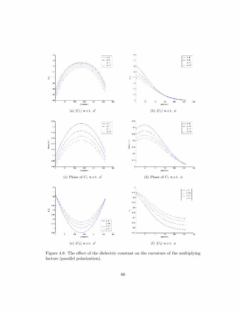
(a) |C1| w.r.t. φ′ (b) |C1| w.r.t. φ
(c) Phase of C1 w.r.t. φ′ (d) Phase of C1 w.r.t. φ
(e) |C2| w.r.t. φ′ (f) |C2| w.r.t. φ
Figure 4.8: The effect of the dielectric constant on the curvature of the multiplyingfactors (parallel polarization).
66
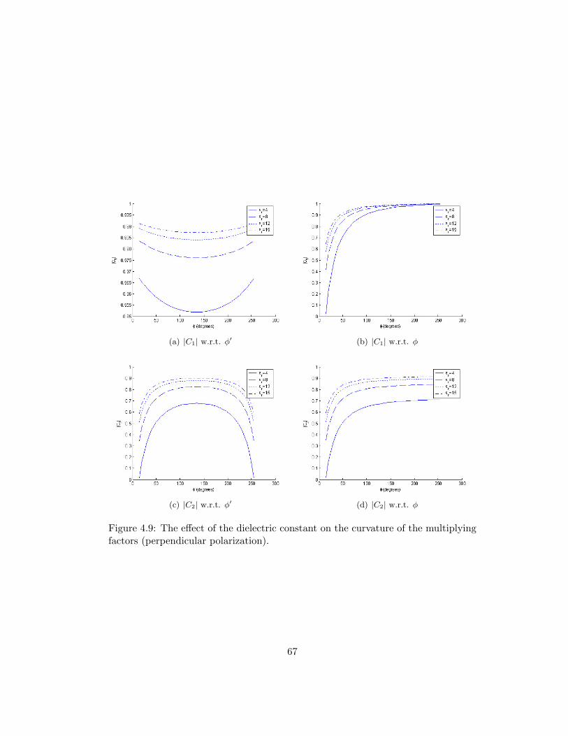
(a) |C1| w.r.t. φ′ (b) |C1| w.r.t. φ
(c) |C2| w.r.t. φ′ (d) |C2| w.r.t. φ
Figure 4.9: The effect of the dielectric constant on the curvature of the multiplyingfactors (perpendicular polarization).
67

less optimally fitted even by using a polynomial of order 3. However, this turns
out to barely degrade the overall accuracy of the construction. On the other hand,
even though the phase of C2 can be reasonably approximated as a constant π, the
magnitude of C2 still plays an important role in determining the value of diffraction
coefficient.
4.5 New S4W with Diffraction
Assume that the two wedge faces are of the same material, and that the sinusoids
are expanded to the fourth significant term in the Taylor’s series. While the com-
putational complexity of the parametric formulation is comparable to that of the
heuristic solutions, the parametric solution can calculate the diffraction field at least
ten times faster than using the rigorous solution. Quantitatively speaking, with the
assumption that one addition takes three cycles and one multiplication takes six
cycles, the total computation time on a 300 MHz microprocessor is less than one
half of a microsecond. Eventually, this approach and other fast computations can
be exploited in real-time wireless channel estimation.
The new method has been incorporated into S4W1.01. Initially, in the in-
tersection test procedure, once a plane is hit, the source ray will be divided into a
reflected ray and a transmitted ray only. In the new version, a wedge list is built
at the beginning and broadcasted to all computational nodes by the master node.
When a beam hits a triangular plane, in addition to initiating a reflected ray and a
transmitted ray, the program detects if the intersection point is on a dielectric wedge
edge. If the intersection point is not on the edge, proceed as usual. If the beam hits
on a wedge edge, the program decides if an unobstructed path exists between the
intersection point and the receiver location based on Keller’s law. That is to deter-
mine if the receiver is in the cone formed by diffracted rays. If a diffracted ray can
reach the receiver, the received field is calculated by tracing back from the receiver
68

location to the transmitter location through the sequence of diffraction, reflections
and transmissions encountered by the beam. If the receiving point is not on the
diffraction cone, no diffracted ray is created. In this manner, only one diffraction is
counted in the ray path searching process. It is found that this treatment is sufficient
because the attenuation by diffraction is big in most of the diffracted angles.
The new version of S4W incorporated with diffraction modeling is released
as S4W1.02. By taking the diffraction effect caused by building edges and corners,
the accuracy of the ray-tracing algorithm is improved.
4.6 Impact of Diffraction in Wideband Modeling
Most of the available literature has so far concentrated on investigating the average
path loss effect by comparing the prediction results with signal strength measure-
ments [4]. However, very few examples exist in terms of wideband propagation
prediction. This could be a nuisance in wireless system emulations because real-
time channel impulse response is not available. This section compares predicted
power delay profiles with wideband measurement results in on-campus buildings.
The measurements made in a campus office building are detailed in [78, 79]. Fig.
4.10 shows the floor plan of the second floor of Whittemore Hall on Virginia Tech
campus. The transmitter is located at the left end of the corridor. Power delay pro-
files received at various locations in the corridor are investigated. Fig. 4.11 shows
the calibration of the prediction using S4W with the measurement campaign at 1.3
GHz. The path loss measurement is -36.9 dB, which is agreeable to the prediction
of -38.2 dB. While the rms delay spread from measurement is 28.5 ns, the rms delay
spread from prediction is 58.3 ns [1]. In order to study the effect of diffraction in
wideband channel modeling, up to 8 reflections, 4 transmissions, and 1 diffraction
are counted in each ray path of the prediction. Fig. 4.12 gives the comparison of
the measurement (MEA), the parametric approach (PAR), and the heuristic method
69

Figure 4.10: Top view of the second floor of Whittemore Hall measured at 1.3 GHzand 4 GHz
70

Figure 4.11: LOS location G measured at 1.3 GHz
(HEU) at an obstructed location H at 1.3 GHz. The path loss from each scheme is
-59.4 dB, -58.4 dB, and -61.0 dB, respectively. Looking at the rms delay spreads, it
turns out that the parametric formulation gives an agreeable delay spread of 30.2
ns to the measured result of 29.9 ns, while the heuristic result is 65.9 ns, having a
far much larger deviation from the measurement. Similarly, Fig. 4.13 gives the
comparison of the measurement, the parametric approach, and the heuristic method
at an obstructed location H at 4 GHz. The path loss from each campaign is -54.6
dB, -54.7 dB, and -59.6 dB, respectively, which shows that parametric method gives
better match to the measurement than the heuristic method. Again, the rms delay
spreads for each campaign are 38.6 ns, 34.8 ns, and 59.0 ns, respectively. From
the above comparisons, it is observed that while both the parametric and heuristic
methods capture the major multipath components, the rms delay spread is predicted
more successfully by the parametric method. Therefore, it is clear that accurate pre-
diction of diffracted field may be important to regenerate real-time channel impulse
responses for future wireless network emulation and analysis.
71

Figure 4.12: Obstructed location H measured at 1.3 GHz
Figure 4.13: Obstructed location H measured at 4 GHz
72

Table 4.3: Measured and predicted path loss, rms delay spread and errorMeas. MEA PAR HEU MEA PAR HEU
PL(dB) PL(dB) (dB) σrms(ns) σrms(ns) (ns)’G’, 1.3 GHz -36.9 -38.2 -38.2 28.5 58.3 58.3’H’, 1.3 GHz -59.4 -58.4 -61.0 29.9 30.2 65.9’H’, 4 GHz -54.6 -54.7 -59.6 38.6 34.8 59.0
4.7 Summary
A new approximation of the diffracted field for right-angle dielectric wedges is pre-
sented using the inverse problem theory. It has been shown that significant im-
provement over existing heuristic formulations can be obtained by polynomial curve-
fitting of the multiplying factors in the UTD diffraction coefficient. The inversely
constructed diffraction coefficient is a reasonable and real-time computable simpli-
fication of the exact solution in the sense that the most important terms in series
expansions of the characterization factors that constitute the diffraction coefficient
are extracted. The parametric formulation of diffraction by a dielectric wedge is 10
times as fast as the rigorous solution provided in [68]. Although the new formulation
is comparable to the heuristic solution in terms of computational complexity, it is
much more accurate than the heuristic solutions. The proposed modeling method of
diffraction has been incorporated in the Site-Specific System Simulator for Wireless
system simulator (S4W ) [62] to improve the accuracy and efficiency of a ray-tracing
predictor. Eventually, this approach and other fast computations can be exploited
in real-time wireless channel estimation.
73

Chapter 5
Urban Propagation Modeling
Using S4W
Path loss characteristics are used to determine the coverage area for a particular
base station in cellular system. Urban areas contain physical obstacles that heavily
influence radio wave propagation and thus shape the coverage area of any wire-
less system. In this aspect, urban environments present significant challenges to
wireless system designers because radio signals interact with buildings, cars, and
other objects that have diverse materials and complex surfaces. Details of the prop-
agation environment may be absorbed into models so that a reasonably compact
representation may be used for design and evaluation of new wireless systems.
This chapter discusses the corner effect in urban environments. The well-
known corner effect phenomenon describes the abrupt change in signal strength
experienced by a mobile user while turning at a corner or going through an in-
tersection. A resource allocation event, e.g., a handoff or a change in modulation
level or transmit power, may be triggered by the corner effect. The signal chang-
ing rate determines how quickly the system must respond. S4W is used to predict
the signal strength at various intersections in the San Francisco financial area and
74

the prediction is compared to the measurement performed by W. M. Smith in the
San Francisco dense urban area [17]. The goal of this chapter is to demonstrate
S4W1.02’s accuracy and extension as a state-of-the-art tool in the field of urban
propagation modeling based on measurements published in [17].
5.1 Introduction
Propagation in a multipath environment is characterized by large, rapid fluctuations
in the received signal strength over space as an object moves through the scene.
Coding and interleaving the bits that are transmitted in a data frame can alleviate
some of the problems encountered by bursty bit errors that occur during a deep
signal fade. Diversity techniques use different observations of the same signal and
combine the results to obtain a composite signal that is of better quality than any of
the constituent signals. The different observation may take place in space, time, or
frequency. These mitigation techniques inherently depend on the stationarity of the
received signal. Interleaving works because only portions of a data frame may be
in error. The technique depends on the fact that the signal is likely to experience a
deep fade for only a short time. After a mobile user turns a corner in a dense urban
area, however, the signal may not increase significantly after the initial fade. This
phenomenon has come to be known as the “corner effect.” Not only does the corner
effect impact the effectiveness of fading mitigation techniques, but there are deeper
system issues involved as well. Since much of the control of mobile wireless systems
is conditioned on the signal quality of each link, the rate of change in the signal
quality determines how rapidly the system must respond before the link quality
deteriorates and the call is dropped.
The objective of this work is to study radio wave propagation in built-up
urban environments and to use the improved S4W to predict the corner effect. The
study is focused on how the city structure influences the estimation of the received
75

signal strength.
5.2 Previous Urban Microcellular Propagation Models
Previous research work has provided some insights in the statistical contributions
of measured path loss for microcellular system design [80,81].
As a result of the intergovernmental framework for European Co-operation
in the field of Science and Technological research, the COST231 study has two
models for urban microcellular propagation, COST231-Hata Model and COST231-
Walfish-Ikegami Model. The COST231-Hata model extends Hata and Okumura
model to 1500-2000 MHz where it is known that the Hata and Okumura model
underestimate path loss. This model can be used to the cases where the base
station (BS) antenna heights are greater than 30 m or surrounding buildings are
well below the BS antenna. It should not be used for small ranges where path loss is
highly dependent on the local topography such as the case of predicting path loss in
urban canyons. The COST231-Walfish-Ikegami Model is applicable to cases where
the BS antenna heights are either below or above the roof tops. It takes into account
parameters such as roof heights, street widths, and street orientations with respect
to radio path. The model works best when the BS antennas are much higher than
the roof tops. It is not very accurate when the BS antennas are about the same
height as the rooftops. It is poor when the BS antennas are much lower than the
rooftops because it does not consider wave guiding in street canyons or diffraction
at street corners.
An empirical street corner path loss model has been proposed by Grim-
lund and Gudmundson [82]. The model assumes LOS propagation until the mobile
reaches a street corner. The NLOS propagation after rounding the street corner
is modeled by assuming LOS propagation from an imaginary transmitter that is
located at the street corner having a transmit power equal to the received power at
76

the street corner from the serving BS.
5.3 Urban Propagation Environment
Urban environments are of practical interest to researchers because of their heavy
impact on radio wave propagation. A typical dense urban area is constituted by tall
buildings situated on a grid-like pattern of streets. In fact, the popularity of wire-
less services in these areas is leading to network congestion. Since adding additional
base stations to extend capacity is an expensive endeavor, deployment engineers
seek ways to extend the capacities of the existing systems. As discussed in the
previous section, one way to extend capacity is through improved resource alloca-
tion methods. Propagation models are important in this regard since they predict
the received signal strength. Although other parameters may be used in resource
allocation decisions, the received signal strength is the fundamental parameter. In
typical cellular systems, control channel signals from active cellular base stations
are transmitted continuously at constant power levels, providing beacons that can
be characterized throughout the coverage area.
The San Francisco financial district is characterized as a dense urban environ-
ment that is constituted by tall buildings situated on a grid-like pattern of streets.
Fig. 5.1 gives the blueprint of the vicinity of the transmitter. The transmitter is
located at 22 Battery Street at an elevation of 173 ft. The AT&T Wireless transmit-
ter antenna operating at 800 MHz is mounted on the north face of a medium-sized
building in the area and is below the rooftops of the surrounding tall buildings.
Since the side streets are flanked by buildings that are taller than the elevation of
the transmitter, the signal energy is likely to propagate around the corners of the
tall buildings rather than over the top of them. Therefore, as shown in Fig. 5.2, the
geometrical shape at the top of each building is simplified and the over the rooftop
effect is neglected.
77

Figure 5.1: Blueprint of the vicinity of the transmitter. The numbers on the mapindicate building heights in feet. The solid lines represent property boundaries.The dashed lines represent the available footprints of the buildings that deviatesignificantly from the property lines. Reprinted from [17] with permission.
78

Figure 5.2: The 3-D plot of the vicinity of the transmitter. All building walls aretreated as planes with a fixed penetration of 10 dB.
79

Fig. 5.2 shows the three-dimensional plot of the vicinity of the transmitter
in an AutoCAD DXF file. All building walls are assumed to be smooth flat surfaces
with average relative permittivity. Building corners are modeled as right angle
wedges for prediction of diffracted field due to these corners. There are more than 40
wedges in the propagation scene shown in the graph. The effect of phenomena such
as scattering and over-rooftop propagation are not yet considered by the model. The
proposed model is not only capable to provide macroscopic quantities like mean field
values and rms delay spread, but also the full wideband channel information, i.e.,
space dependent complex channel responses with a high time dispersion resolution.
5.4 Corner Effects in Dense Urban Streets
Because Battery Street is aligned primarily with the transmitter, there are a large
number of waveguide modes that propagate down the street. For the intersections
along Battery Street, this rich mixture of modes contributes to the gradual rolloff
at the street corners and to the pointed peak in the signal strength within the
intersection.
The intersections that most clearly exhibit the corner effect are the intersec-
tions with streets that cross the main radial streets from the transmitter (Battery
and Bush/Pine). Along Montgomery Street, in addition to the primary radial streets
from the transmitter, there are several cross streets (Bush, California, and Sutter)
that have strong enough signals for the strength in the intersections to rise above
the large-scale fading. A street’s perpendicular distance to the transmitter will de-
termine whether it is the inlet to or the outlet from the intersection. The inlet street
is the street that has the shorter distance to the transmitter and is the street from
which the signal enters the intersection. The signal flows from the intersection to
the outlet street, which has a larger distance to the transmitter. This general rule
helps explain why the corner effect is usually exhibited along cross streets to the
80

Corner Location Cross-Correlation rms errorCoefficient ρ (dB)
California at Battery 0.87 13.3Sacramento at Battery 0.95 12.7Montgomery at Pine 0.92 17.7Montgomery at Bush 0.85 8.8Montgomery at Sutter 0.74 24.3
Sansome at Pine 0.92 11.0
Table 5.1: Cross-correlation coefficients of prediction and measurement at variousstreet corners
main radial streets from the transmitter. For these intersections, there is a large
difference in the distance for each of the streets.
Several intersections along Montgomery Street exhibit the corner effect. The
transmitter is lined up most closely with Battery Street and is not located exactly at
the intersection with Pine Street. The signal from Battery Street is strong enough
to feed over into the cross streets (California, Bush, and Sutter).
5.4.1 Comparisons of Predictions and Measurements
In this chapter, the predictions are compared to the measurements. In the prediction
throughout this chapter, the transmit frequency is 800 MHz (λ = 0.375 m). The
averaging window is chosen to be about 20λ. The predicted and measured corner
effects are compared with cross correlation coefficient that is defined by
ρ =E[X − E[X]]E[Y − E[Y ]]
σXσY(5.1)
where E[ ] denotes the expected value and σ represents standard deviation.
Table 5.1 shows various cross correlation coefficients computed using Eq.
5.1. Most of the correlation coefficients are greater than 0.75, exhibiting a good
agreement between the predictions and measurements.
81

5.4.2 Multipath Channel Parameters
Wide-band multipath channels can be grossly quantified by their mean excess delay
τ and rms delay spread στ [21]. The mean excess delay is the first moment of power
delay profile and is defined to be
τ =∑N
i=1 Piτi∑Ni=1 Pi
(5.2)
where Pi and τi are the power and delay of the ith multipath component of a PDP,
respectively, and N is the total number of multipath components. The rms delay
spread is the square root of the second central moment of the power delay profile
and is defined to be
στ =√
τ2 − τ2 (5.3)
where
τ2 =∑N
i=1 Piτ2i∑N
i=1 Pi
(5.4)
The delays of each profile are the temporal intervals relative to the multipath
component arriving at τ1 = 0. The cumulative distribution functions (cdf’s) of the
rms delay spread at street intersections on Montgomery Street is obtained based
on the prediction result and shown in Fig. 5.3, where στ is computed for each
individual power delay profile at each location. The median values of rms delay
spread at Pine (157 ns) and Bush (160 ns) are greater than those at California (58
ns) and Sutter (64 ns). Fig. 5.4 gives the distributions of number of multipath
components on Montgomery, including the distribution along Montgomery and at
intersections with California, Pine, Bush, and Sutter. Nearly all of the cdf’s exhibit
symmetry about the mean. Obviously, the distribution along the entire Montgomery
street has the largest standard deviation. As the corner effects at Pine and Bush
are stronger than those at California and Sutter, the medians at Pine (70) and Bush
82

Locations mean (ns) median (ns) std (ns)Along Montgomery 150.3 140.5 102.3
Montgomery at California 72.8 57.9 37.1Montgomery at Pine 164.6 156.6 113.2Montgomery at Bush 169.8 159.9 63.9Montgomery at Sutter 84.1 63.7 80.2
Table 5.2: Distribution of rms delay spread of predicted profiles on Montgomery
(57) are greater than those at California (27) and Sutter (13).
Figure 5.3: Cumulative distribution functions of rms delay spread at various streetintersections on Montgomery.
5.4.3 Corner Effect at A Radial Street (Battery)
Figs. 5.5 and 5.6 show the corner effect at the intersections of a radial street (Bat-
tery) relative to the transmitter. The predictions on California and Sacramento are
agreeable to the measurements, giving a high cross-correlation coefficient of 0.87
and 0.95 respectively. It is conceived that the waveguid effect in street canyons is
dominant particularly on the main radial street with respect to the transmitter. As
83

Figure 5.4: Cumulative distribution functions of number of multipath componentsreceived in an individual profile for profiles predicted at discrete λ/3 on Montgomery.
Locations mean median stdAlong Montgomery 53 46 30
Montgomery at California 29 27 12Montgomery at Pine 59 70 31Montgomery at Bush 59 57 22Montgomery at Sutter 16 13 11
Table 5.3: Distribution of number of multipath components on Montgomery
84

Figure 5.5: Corner effect on California at Battery. The prediction (solid) has a highcross correlation with the measurement (dashed).
pointed in [17], a roll-off in signal strength at street corners indicates that a concen-
tration of energy in the lower-order modes which experience fewer reflections along
the radial street produces less coupling into the side streets. Higher-order modes
correspond to rays that bounce back and forth much more between the buildings
along the street. Therefore, higher-order modes tend to couple into the side streets
so that a gradual roll-off in signal strength is exhibited.
5.4.4 Corner Effect on Cross Streets (Montgomery and Sansome)
Along a cross street with respect to the transmitter, the wave guiding effect is not
obvious. This is different from the indoor hallway case in which the coupling of
higher-order modes and lower-order modes suffices to interpret the signal variation
trend along the hallway [83]. Penetration through building walls and diffraction
via building corners combine to play indispensable role in determining the large-
scale variation of the received signal strength along a cross street. In fact, the
correct fading characteristics is not properly captured with building wall penetration
85

Figure 5.6: Corner effect on Sacramento at Battery. The prediction (solid) has ahigh cross correlation with the measurement (dashed).
suppressed.
Fig. 5.7 gives an illustration of how different number of transmissions affect
the prediction. The prediction is taken along the Montgomery street that intersects,
from south to north, Sutter, Bush, Pine, and California (each of the cross streets
is denoted by two vertical dotted lines). The maximum number of reflections is 8
and the maximum number of transmissions varies from 0 to 6. Only 1 diffraction
is counted in the ray-tracing procedure. The received signal strength is averaged
using a rectangular window with a size of 20λ.
It is observed that the prediction is not adequate if only reflections are
counted. According to the measurement results, although not all intersections ex-
hibit the corner street, the phenomenon is still significant at all four intersections.
However, with transmissions suppressed in the predictions, the street corner effect
is only observed at the intersections of Pine and Bush, and is smeared as at Cal-
ifornia and Sutter. It turns out that the coupling of waveguide modes with more
reflections in the street canyons does not make significant contribution to received
86

Figure 5.7: Effect of transmission on propagation predictions on Montgomery Street.
87

signal strength on the streets that are fairly apart from the transmitter. Therefore,
in order to obtain reasonable prediction results, the threshold of number of trans-
missions should be at least 2 or even 4. Although the predicted signal strength at
the intersections is lower than the measurements, which is possibly caused by the
inaccuracy of the database, the correlation coefficients in Table 5.1 show effective
prediction using the prediction model.
Table 5.1 also shows the corner effect on a closer cross street Sansome at Pine.
The signal on Pine is strong enough to feed over Battery and reaches Sansome. It
is found that for streets that are close to the transmitter, reflections play the most
significant role in determining the received signal strength and transmissions could
be neglected. This phenomenon indicates a “quasi-indoor” wave guiding effect.
In fact, most of the future PCS microcellular systems are expected to operate
in the 1800-2000 MHz frequency bands. Some studies have suggested that path losses
experienced at 1900 MHz are approximately 10 dB larger than those at 900 MHz
where all other parameters are kept constant. As discussed in the previous section,
transmissions through buildings make significant contributions to the signal strength
received on Montgomery street since it is a cross street relative to the transmitter.
As higher frequency waves experience more attenuation than lower frequency ones,
it is foreseeable that the corner effect in higher frequency bands at the intersections
on Montgomery streets is not as severe as in lower frequency bands.
5.4.5 Effect of Electrical Parameters
The ray tracing model in S4W is dependent on the electrical parameters attributed
to the building walls. Variations of three units of the relative permittivity could lead
to completely erroneous predictions. The predictions are more sensitive when the
permittivity is low. Furthermore, constant loss per reflection or transmission leads
to less satisfactory predictions than the computations using the Fresnel reflection
88

coefficient that depends on the incident angle.
5.5 Summary
This chapter studies the corner effect at various street intersections in a typical
dense urban area. Predictions show that the wave-guiding effect of street canyon
is only applicable to the radial street or close cross streets to the transmitter. In
these cases, various modes of reflections make most important contribution to the
received signal strength. While at the intersections on cross streets fairly apart from
the transmitter, transmission is not negligible. Instead, it plays an important role
in forming the street corner effect.
89

Chapter 6
Channel Characterization for
MIMO Wireless
Communications
6.1 Introduction
Multiple-input-multiple-output (MIMO) wireless systems use multiple antenna ele-
ments at the transmitter and receiver to offer improved capacity over single antenna
topologies in multipath channels. In such systems, the antenna properties as well
as the multipath channel characteristics play a key role in determining communica-
tion performance. Research issues concerning antennas and propagation in MIMO
systems include channel capacity computation, channel measurement and modeling
approaches, and the impact of antenna element properties and array configuration
on system performance [84]. While coding and signal processing are key elements
to successful implementation of a MIMO system, considerable research has been
devoted recently to propagation channel and antenna design since these two ar-
eas represent major parameters that ultimately impact system performance. For
90

Figure 6.1: A MIMO system with M transmit antennas and N receive antennas.
instance, assessing the potential of MIMO systems requires a new level of under-
standing of multipath channel characteristics. Even when extensive information
concerning the behavior of antenna diversity in multipath channels is available, new
issues have come up about the impact of antenna properties and array configuration
on system performance.
With the growing interest in implementing MIMO communication systems,
evaluation of MIMO channel capacity in typical and realistic propagation environ-
ments has become important. The goal of this chapter is to focus on MIMO channel
capacity computation and spatial correlation through the S4W wideband propa-
gation modeling approach and wideband channel measurement. Throughout this
chapter, matrices and column vectors are represented as boldface uppercase and
lowercase letters, respectively, Hij is the element occupying ith row and j th column
of the matrix H, and hi is the ith element of the vector h.
91

6.2 MIMO System Capacity
MIMO wireless sytems, characterized by multiple antenna elements at the trans-
mitter and receiver, have demonstrated the potential for increased capacity in rich
multipath environments [85–88]. Such systems operate by exploiting the spatial
properties of the multipath channel, thereby offering a new dimension which can be
used to enable enhanced communication performance.
For linear channel elements, the continuous-time baseband waveforms x(ω)
(ω is frequency) is fed to the NT channel inputs and the channel H(ω) combines
the input signals to obtain the NR element output (receive) waveform vector y(ω).
Therefore, the MIMO channel input-output relationship may be written as
y(ω)︸ ︷︷ ︸NR×1
= H(ω)︸ ︷︷ ︸NR×NT
x(ω)︸ ︷︷ ︸NT×1
+ η(ω)︸ ︷︷ ︸NR×1
(6.1)
where η(ω) is additive noise produced by the channel (interference plus noise from
the RF front end) and the matrix dimensions are as specified. Each element Hij(ω)
represents the transfer function between the j th transmit and ith receive antenna.
It is convenient to define a single metric that captures both the signal-to-
noise ratio (SNR) and multipath spatial characteristics to represent the quality of the
MIMO channel. The Shannon channel capacity has emerged as the de facto measure
of choice for MIMO system analysis [89]. Intuitively, this quantity represents the
highest error-free MIMO transmission rate for a given transfer matrix under optimal
space/time-coding and modulation. Since MIMO is a narrowband concept where
the assumption of flat fading holds, the majority of the channel capacity expressions
are given for the narrowband case. Yet the wideband case or the frequency selective
channel is seen to provide diversity gain and hence higher capacity.
The expressions for MIMO capacity as well as MISO, SIMO, and SISO capac-
ity are included in [86]. These were derived under a number of assumptions, which
92

include narrowband Rayleigh channel during a data burst, channel knowledge at
the receiver, additive white Gaussian noise and total transmitted power remains the
same regardless of the number of transmit antennas. Under these assumptions, the
capacity represents the transmission rate per Hertz of bandwidth (bits/s/Hz).
As originally stated in [86], when the channel is unknown to the transmitter
but perfectly known to the receiver, and the transmit power is equally allocated to
all antenna elements, the achieved capacity of a narrowband nR×nT MIMO system
is given by
C(t, f) = log2
(det
(InR +
ρ
nTH(t, f)HH(t, f)
))(6.2)
where InR ∈ CnR×nT is the identity matrix, ρ is the average SNR at each receiver
branch over the whole bandwidth, H(t, f) ∈ CnR×nT is the normalized time-varying
MIMO channel matrix for frequency f and (·)H denotes matrix conjugate transpose.
For the frequency selective channel the capacity is given as the integral of the
narrowband channel [90]. Wideband capacity, normalized to bandwidth W , may be
obtained by integrating C(t, f) over the frequency domain:
C =1W
∫log2 det
(InR +
ρ
nTH(t, f)HH(t, f)
)df (6.3)
Since there are F distinct frequency samples available, integration degenerates to
the sum as
C(t) =1W
F∑f=1
log2 det(InR +
ρ
nTH(t, f)HH(t, f)
)(6.4)
where ∆f = W/F is the frequency separation of tones. The normalized channel
matrix H(t, f) is obtained by applying a normalization factor to the measured data
H(t, f), i.e.,
H(t, f) = H(t, f)/
√√√√ 1nRnT F
nR∑i=1
nT∑j=1
F∑k=1
|Hij(t, fk)|2 (6.5)
93

MIMO systems assume a rich scattering environment. The number of scat-
terers limits the MIMO channel capacity. In the case of a single LOS path, the
channel capacity is a function of range and the antenna geometry [91]. When a
LOS component is present with other scattered components the channel becomes
Rician and in this case the capacity is a function of the Rician factor [92]. Another
situation which results in a low rank matrix is known as the keyhole effect which
arises when the channel matrix is not correlated, such as in the case of transmission
in a tunnel, along a corridor or over roof top diffraction. This can be remedied using
horizontal polarization for reception for a vertical polarization transmission.
6.3 MIMO Channel Characterization using S4W
6.3.1 Previous work
Assessing the performance of MIMO systems in realistic environments requires a
detailed description of the multipath channel. This description must go beyond tra-
ditional models or measurement campaigns, as a matrix of transfer functions must
be accurately represented. In some cases, channel measurements are used to fully
characterize these channels. Most of the measurements for MIMO system evaluation
are in the 1.9-2.5 GHz band and the 5.2 and 5.8 GHz bands. The 5.2 and 5.8 GHz
cover picocells either in indoor environments, in hotspots, or in outdoor stationary
environments [93]. The 1.9 - 2.5 GHz measurements are mainly outdoor measure-
ments in urban and suburban environments carried out by Lucent and Stanford
University [94].
Since relatively few measurement campaigns have been performed and the
resulting data is not widely available, researchers have turned to channel models
that capture the key behaviors observed in the experimental data, which facilitate
performance assessment of potential space-time coding approaches in realistic prop-
94

agation environments.
As discussed in previous chapters, ray-tracing prediction has emerged as the
most popular solution for the analysis of site-specific scenarios due to its ability to
analyze very large structures with reasonable computational resources. The tech-
nique is based on geometrical optics, supplemented by diffraction theory to enhance
accuracy in shadowed regions. Existing ray-tracing techniques have demonstrated
reasonable accuracy in predicting large-scale path loss variation, with error standard
deviations of 3-7 dB being reported. However, perhaps due to oversimplification
of the geometrical scenario representation, preliminary comparisons of ray-tracing
predictions with measurements indicate that the simulations tend to underestimate
MIMO channel capacity [95]. Other work shows promising agreement in exact delay
of arrivals (DOAs) of measured and simulated microcells. In this case, the results
can be combined with uniformly distributed phases to regenerate wireless channel
impulse responses [96–99]. Ray-tracing predictions have been used to study MIMO
channel characteristics such as spatial-signature variation with small-scale move-
ment [100], capacity variation with array location and antenna spacing [101, 102],
and angular clustering of multipath arrivals [103]. More recently the effects of diffuse
scattering and diffraction on the MIMO channel capacity have been studied [12,104]
and it is shown that scattering and diffraction effects from metal frames, complex
walls, and leaves of trees lead to varying fading characteristics and increase of pre-
dicted MIMO capacity.
Although ray-tracing studies have led to the development of simpler statisti-
cal models, it is conceived that site-specific knowledge is essential for future wireless
system design. Therefore, in the following section of this chapter, we are going
to investigate how much model detail is needed to correctly represent the MIMO
channel characteristics.
95

Figure 6.2: A floor print of the propagation scenario on the Pickle Research Centercampus at UT-Austin. The primary feature is characterized by one- and two-storybuildings.
6.3.2 Propagation Scenario
Fig. 6.2 gives the propagation scene as part of the floor plan of the Pickle Research
Center (PRC) campus at the University of Texas at Austin. The campus is a typical
suburban environment spotted with about 50 one- or two-story buildings on grass-
covered ground. The transmitter is located on the rooftop of a one-story laboratory
building and thus it is approximately 15 m above ground level. The receiver is
placed 0.6 m above the ground near a one-story building. The Tx-Rx distance is
about 257 m. It is shown that the transmitter and receiver were separated by two
buildings. A LOS path does not exist.
96

0.8 1 1.2 1.4 1.6 1.8 2 2.2 2.4
−150
−145
−140
−135
−130
−125
−120
−115
−110
time delay (µs)
Rec
eive
d po
wer
(dB
m)
Figure 6.3: An example of the power delay profile predicted using S4W for one pairof antenna elements.
A 4× 8 MIMO system with vertical polarized dipole antenna elements oper-
ating at 1.8 GHz is input to the ray-tracer. The inter-element spacing is chosen to
be λ for the transmitter and 0.5λ for the receiver.
6.3.3 Wideband Capacity Results
Fig. 6.3 gives a snapshot of the predicted PDP for one antenna pair in the 4 × 8
MIMO system. Fig. 6.4 shows the mean capacity as a function of the average
SNR ρ for various MIMO systems. The concave shape of the curves indicates that
the simulation tends to underestimate the MIMO capacity. This could result from
the oversimplification of the geometric scenario in the propagation environment.
Some scatterers such as pipes and fences are not considered in the intersection test
procedure.
97

Figure 6.4: Predicted mean capacity vs. ρ for various MIMO systems. (txspace =λ, rxspace = 0.5λ)
Figure 6.5: Spatial correlation of the received power by comparison between S4Wsimulation and Rayleigh fading (according to [105]).
98

6.4 Spatial Correlation
The spatial correlation corresponding to a discrete scanning of the field along a line
is defined in the following way. Let P (i), i = 1..., N be the predicted samples along
line l and Pm the corresponding average value. We define
C(k) =∑N−k
i=1 (P (i)− Pm)(P (i + k)− Pm)∑N−ki=1 (P (i)− Pm)2
(6.6)
as the discrete spatial correlation over line l, which is a function of the distance
index k. It corresponds to a continuous spatial correlation at the normalized dis-
tance k∆s/λ, with ∆s being the scanning step along the line (1.67 cm here). The
simulation spatial correlation result refers to the environment shown in Fig. 6.2.
The transmitter is located as shown in the graph. The receiver has been placed
initially on the location denoted by “Rx” and then several field scans along lon-
gitudinal lines in the environment have been performed with a resolution of 1.67
cm. By computing the spatial correlation for all scans and then averaging point
by point, an overall spatial correlation function is obtained which depends only on
the environment and on transmitter location. The computed result is compared
with the theoretical curve for the case of a Rayleigh-fading channel with uniform
angle of arrival [105] in Fig. 6.5. It is evident that the estimated correlation is
always greater than the theoretical one. This is probably due to the strong direct
or wall-transmitted path between Tx and Rx, and to a nonuniform distribution of
the angle of arrival. The computed spatial correlation is in good agreement with
the theoretical one. This suggests that the ray-tracing modeling in S4W is capable
of faithfully reproducing the statistics of the fast fading (if not its exact shape) and
can be therefore considered a reliable and convenient tool for diversity performance
evaluation.
99

6.5 Summary
It is well known that channel capacity can be greatly increased by using antenna
array at both the transmit and receive sides as long as the environment can pro-
vide sufficient scattering. This chapter explores the MIMO channel capacity in
a suburban environment with both site-specific prediction results at 1.8 GHz. In
the 4 × 8 MIMO system, the spacing between two neighboring antenna elements
is 0.5λ at the receiver side and λ at the transmitter side. The capacity results
show that site-specific prediction tends to underestimate the MIMO channel capac-
ity. This could be the oversimplification of the building geometry and omission of
other scatterers existing in the propagation scene. Another interesting result is that
three-dimensional RT/UTD model is able to reproduce spatial fading statistics and
therefore can be used to evaluate diversity performance.
100

Chapter 7
Concluding Remarks
7.1 Conclusions
This dissertation first surveys site-specific propagation modeling techniques and
identifies the challenges to improving the existing ray-tracing based modeling meth-
ods. The contributions of the dissertation can be categorized in three groups.
The first contribution is focused on mathematical modeling for propagation
prediction and a new diffraction construction is developed for real-time channel mod-
eling. It has been shown that the commonly used heuristic diffraction coefficient
(i.e., Luebbers’) can lead to inaccurate results in the estimation of diffracted field.
This dissertation proposes a new method to formulate the UTD diffraction coeffi-
cient by least square polynomial curve fittings. This new approach can be denoted
as the parametric formulation of diffraction coefficient (PFD). This solution is valid
for right-angle dielectric wedges and for both parallel and perpendicular field polar-
izations. The proposed solution has about the same computational efficiency as the
commonly used solutions. As the parametric coefficients can be computed offline
in advance and possibly downloaded to mobile devices over the air or computed
in the device itself, this formulation enables more accurate and faster evaluation
101

of diffracted field by building edges in radio wave propagation modeling, and may
enable real-time prediction.
The second contribution is the addition of the PFD diffraction model to
the S4W software. The new improved S4W with diffraction provides a significant
improvement for the public domain software that has been funded by the NSF grant.
The third contribution is the investigation of the impact of propagation mech-
anisms on the street corner effect in dense urban environment. The S4W ray-tracing
prediction modeling method is applied and validated with measurements at 800
MHz in the San Francisco financial area. Cross-correlation of the predicted and the
measured signal strengths has been calculated at different street intersections and
correlation coefficients of higher than 0.8 are achieved where corner effect occurs.
Further investigations show that the waveguide effect in the street canyon is only
applicable to the propagation phenomena in radial streets with respect to the trans-
mitter. While in the case of cross streets that are not close to the transmitter, the
transmission mechanism makes significant contribution to received signal variations.
Finally, the S4W site-specific prediction capability is applied to the campus
of Pickle Research Center at UT-Austin to study the MIMO channel characteristics.
The prediction using a 4× 8 MIMO system operating at 1.8 GHz shows that S4W
is able to reproduce fading statistics and that the estimation of MIMO channel
capacity using site-specific prediction is dependent on the accuracy of the input
environment.
7.2 Future Directions
The results reported in this dissertation open new avenues for further research.
There are several aspects that are worth exploring.
First, in combination with wideband measurements, the new formulation of
diffraction can be employed to study canonical cases such as typical propagation
102

scenarios where diffraction plays a pivotal role in received signal strength. Further-
more, the nonlinear optimization criterion adopted in computing the parametric
coefficients for diffraction coefficient can be improved so as to decrease the error in
the inverse solution from the rigorous value.
More work is needed in accelerating the ray-tracer in the preprocessing stage.
Currently, S4W still conducts an exhaustive (brute force) search of ray-paths. The
future trend is to apply more efficient algorithms such as angular Z-buffer technique
to the ray-path search algorithm so that the number of intersection tests on the
ray paths can be reduced. As a parallel computing ray-tracer, S4W not only relies
on message passing interface libraries for multiprocessor communication but also
employs various computer science techniques such as database interface control,
balance loading algorithms, etc. As the ultimate long-term goal of this research
is to realize site-specific radio, the software package is yet to be converted into
a single-processor based, compact and portable program. A hybrid method that
utilizes statistical spatial geometry could be a feasible solution.
Finally, implementation issues of MIMO communication systems have be-
come popular research topics recently. In order to determine major parameters that
ultimately impact MIMO system performance, site-specific prediction tools can be
utilized to explore the properties of the physical multipath propagation channel.
MIMO channel characteristics such as spatial-signature variation with small-scale
movement, channel temporal and spatial correlations, capacity variation with array
location and antenna spacing and angular clustering of multipath arrivals can be
studied using ray-tracing simulations.
103

Bibliography
[1] S. Y. Seidel and T. S. Rappaport, “Site-specific propagation prediction for
wireless in-building personal communication system design,” IEEE Trans.
Veh. Technol., vol. 43, no. 4, pp. 879–891, November 1994.
[2] S. Y. Tan and H. S. Tan, “A microcellular communications propagation model
based on the uniform theory of diffraction and multiple image theory,” IEEE
Trans. Antennas Propagat., vol. 44, no. 10, pp. 1317 – 1326, October 1996.
[3] C. Yang, B. Wu, and C. Ko, “A ray-tracing method for modeling indoor wave
propagation and penetration,” IEEE Trans. Antennas Propagat., vol. 46, no. 6,
pp. 907–919, June 1998.
[4] J. H. Tarng, W. Liu, Y. Huang, and J. Huang, “A novel and efficient hy-
brid model of radio multipath-fading channels in indoor environments,” IEEE
Trans. Antennas Propagat., vol. 51, no. 3, pp. 585–594, March 2003.
[5] S. Shakkottai, T. S. Rappaport, and P. C. Karlsson, “Cross-layer design for
wireless networks,” IEEE Communications Magazine, vol. 41, no. 10, pp. 74–
80, October 2003.
[6] T. S. Rappaport, “Site-specific knowledge for next generation wireless net-
works,” IEEE 802.11-04-1478-00-0wng, November 2004.
104

[7] T. S. Rappaport, C. Na, and J. Chen, “Application throughput measure-
ments and predictions using site-specific information,” IEEE 802.11-04-1473-
00-000t, November 2004.
[8] A. Lauer, A. Bahr, and I. Wolff, “Fdtd simulations of indoor propagation,”
Proceedings of the 44th IEEE Vehicular Technology Conference, pp. 883–886,
1994.
[9] A. Lauer, I. Wolff, A. Bahr, J. Pamp, and J. Kunisch, “Multi-mode fdtd
simulations of indoor propagation including antenna properties,” Proceedings
of the 45th IEEE Vehicular Technology Conference, pp. 454–458, 1995.
[10] J. Litva, C. Wu, and A. Ghaforian, “Use of fdtd for simulating the angle of ar-
rival and time delay of signals propagating in indoor environments,” Electronic
Letters, pp. 930–932, May 1996.
[11] R. P. Torres, L. Valle, and M. Domingo, “Computer tool to analyze radio
channel in arbitrary enclosed spaces using ray tracing,” Proceedings of the
48th IEEE Vehicular Technology Conference, pp. 581–585, May 1998.
[12] Z. Yun, M. F. Iskander, and Z. Zhang, “Complex-wall effect on propagation
characteristics and mimo capacities for an indoor wireless communication en-
vironment,” IEEE Trans. Antennas Propagat., vol. 52, no. 4, pp. 914–922,
April 2004.
[13] V. Rodoplu and T. H. Meng, “Minimum energy mobile wireless networks,”
IEEE JSAC, vol. 17, no. 8, pp. 1333–1344, August 1999.
[14] R. J. Punnoose, P. V. Nikitin, J. Broch, and D. D. Stancil, “Optimizing wire-
less network protocols using real-time predictive propagation modeling,” IEEE
Radio and Wireless Conference, pp. 39–44, August 1999.
105
[15] A. Verstak, N. Ramakrishnan, L. T. Watson, J. He, C. A. Shaffer, K. K.
Bae, J. Jiang, W. H. Tranter, and T. S. Rappaport, “BSML: a binding
schema markup language for data interchange in pses,” Scientific Program-
ming, vol. 11, no. 3, pp. 199–224, March 2003.
[16] T. S. Rapport, J. C. Browne, N. Ramakrishnan, S. Shakkottai, and
S. Varadarajan, “Montage: an integrated end-to-end design and development
framework for wireless networks,” NSF Grant Number 0305644, 2003-2006.
[17] W. M. Smith, “Urban propagation modeling for wireless systems,” Ph.D. dis-
sertation, Stanford University, February 2004.
[18] D. J. Cichon and T. Kurner, Cost 231 Final Rep. Web:
http://www.lx.it.pt/cost231/, 1998, ch. 4, pp. 115 – 202.
[19] G. L. Turin, “A statistical model for urban multipath propagation,” IEEE
Transactions on Vehicular Technology, vol. VT-21, no. 1, pp. 1–9, 1972.
[20] J. B. Andersen, T. S. Rappaport, and S. Youshida, “Propagation measurement
and models for wireless communications channels,” IEEE Communications
Magazine, vol. 33, no. 1, pp. 42–49, February 1995.
[21] T. S. Rappaport, Wireless Communications: Principles and Practice, 2nd ed.
Upper Saddle River, NJ 07458: Prentice Hall, 2002, ch. 4 and 5.
[22] K. A. Chamberlain and R. J. Leubbers, “An evaluation of longley-rice and gtd
propagation models,” IEEE Trans. Antennas Propagat., vol. AP-30, no. 6, pp.
1093–1098, November 1982.
[23] J. B. Keller, “Geometrical theory of diffraction,” Journal of the Optical Society
of America, vol. 52, no. 2, pp. 116–130, February 1962.
106

[24] R. G. Kouyoumjian and P. H. Pathak, “A uniform geometrical theory of
diffraction for an edge in a perfectly conducting surface,” Proc. IEEE, vol. 62,
no. 11, pp. 1448–1461, November 1974.
[25] R. J. Luebbers, “Finite conductivity uniform UTD versus knife diffraction
prediction of propagation path loss,” IEEE Trans. Antennas Propagat., vol. 32,
pp. 70–76, January 1984.
[26] J. B. Keller, “The geometrical theory of diffraction,” Proceedings of the Sympo-
sium on Microwave Optics, June 1953, eaton Electronics Research Laboratory,
McGill University, Montreal, Cannada.
[27] H. R. Anderson, “A ray-tracing propagation model for digital broadcast sys-
tems in urban areas,” IEEE Trans. Broadcast., vol. 39, no. 3, pp. 309–317,
Semptember 1993.
[28] K. Rizk, J. Wagen, and F. Gardiol, “Two-dimensional ray-tracing modeling
for propagation prediction in microcellular environments,” IEEE Trans. Veh.
Technol., vol. 46, no. 2, pp. 508–518, May 1997.
[29] C. Demetrescu, C. C. Constantinou, and M. J. Mehler, “Corner and rooftop
diffraction in radiowave propagation prediction tools: a review,” VTC, pp.
515–519, 1998.
[30] K. A. Remley, H. R. Anderson, and A. Weisshar, “Improving the accuracy of
ray-tracing techniques for indoor propagation modeling,” IEEE Trans. Veh.
Technol., vol. 49, no. 6, pp. 2350–2358, November 2000.
[31] D. A. McNamara, C. W. I. Pistorius, and J. A. G. Malherbe, Introduction
to the Uniform Geometrical Theory of Diffraction. Norwood, MA: Artech
House, 1990.
107

[32] C. Bergljung and L. G. Olsson, “Rigorous diffraction theory applied to steet
microcell propagation,” Proc. GLOBECOM ’91, pp. 1292 – 1296, 1991.
[33] P. D. Holm, “Utd-diffraction coefficients for higher order wedge diffracted
fields,” IEEE Trans. Antennas Propagat., vol. 44, no. 6, pp. 879–888, June
1996.
[34] L. E. Vogler, “An attenuation function for multiple knife-edge diffraction,”
Radio Science, vol. 17, no. 6, pp. 1541–1546, November-December 1982.
[35] J. B. Andersen, “UTD multiple-edge transition zone diffraction,” IEEE Trans.
Antennas Propagat., vol. 45, no. 7, pp. 1093–1097, July 1997.
[36] ——, “Transition zone diffraction by multiple edges,” Proc. Inst. Elect. Eng.,
Microwave Antennas Propagat., vol. 141, no. 5, pp. 382–384, October 1994.
[37] C. Tzaras and S. R.Saunders, “An improved heuristic utd solution for multiple-
edge transition zone diffraction,” IEEE Trans. Antennas Propagat., vol. 49,
no. 12, pp. 1678–1682, December 2001.
[38] M. F. Iskander and Z. Yun, “Propagation prediction models for wireless com-
munication systems,” IEEE Trans. Microwave Theory Tech., vol. 50, no. 3,
pp. 662–673, March 2002.
[39] S. Y. Tan and H. S. Tan, “Utd propagation model in an urban street scene
for microcellular communications,” IEEE Trans. Energy Conversion, vol. 35,
no. 4, pp. 423–428, November 1993.
[40] V. Erceg, J. A. J. Rustako, and R. S. Roman, “Diffraction around corners and
its effects on the microcell coverage area in urban and suburban environments
at 900 mhz, 2 ghz, and 6 ghz,” IEEE Trans. Veh. Technol., vol. 43, no. 3, pp.
762 – 766, August 1994.
108

[41] W. Zhang, “Fast two-dimensional diffraction modeling for site-specific prop-
agation prediction in urban microcellular environments,” IEEE Trans. Veh.
Technol., vol. 49, no. 2, pp. 428–436, March 2000.
[42] H. M. El-Sallabi, G. Liang, H. L. Bertoni, I. T. Rekanos, and P. Vainikainen,
“Influence of diffraction coefficient and corner shape on ray prediction of power
and delay spread in urban microcells,” IEEE Trans. Antennas Propagat.,
vol. 50, no. 5, pp. 703 – 712, May 2002.
[43] M. C. Lawton and J. P. McGeehan, “The application of a deterministic ray
launching algorithm for the prediction of radio channel characteristics in small-
cell environments,” IEEE Trans. Veh. Technol., vol. 43, pp. 955–969, Novem-
ber 1994.
[44] J. H. Tarng, W. R. Chang, and B. J. Hsu, “Three-dimensional modeling of 900-
mhz and 2.44-ghz radio propagation in corridors,” IEEE Trans. Veh. Technol.,
vol. 46, no. 2, pp. 519–527, May 1997.
[45] S. Y. Tan and H. S. Tan, “Propagation model for microcellular communication
sapplied to path loss measurements in ottawa city street,” IEEE Trans. Veh.
Technol., vol. 44, no. 2, pp. 313 – 317, May 1995.
[46] S. Y. Tan, M. Y. Tan, and H. S. Tan, “Multipath delay measurements and
modeling for interfloor wireless communications,” IEEE Trans. Veh. Technol.,
vol. 49, no. 4, pp. 1334–1341, July 2000.
[47] A. S. Glassner, An Introduction to Ray Tracing. San Diego, CA: Academic,
1989.
[48] G. Durgin, N. Patwari, and T. S. Rappaport, “Improved 3d ray launching
method for wireless propagation prediciton,” Electronics Letter, vol. 33, no. 16,
pp. 1412–1413, 1997.
109

[49] M. Dottling, T. C. Becker, and W. Wiesbeck, “Modeling of the dect outdoor
radio channel,” Proceedings of the 47th IEEE Vehicular Technology Confer-
ence, pp. 1947–1951, May 1997.
[50] R. P. Torres, L. Valle, and M. Domingo, “Computer tool to analyze radio
channel in arbitrary enclosed spaces using ray tracing,” Proceedings of the
48th IEEE Vehicular Technology Conference, pp. 581–585, May 1998.
[51] M. F. Catedra, J. Perez, F. S. de Anana, and O. Gutierrez, “Efficient ray-
tracing techniques for three-dimensional analyses of propagation in mobile
communications: Application to picocell and microcell scenarios,” IEEE An-
tennas and Propagations Magazine, vol. 40, pp. 15–28, April 1998.
[52] F. S. de Adana, O. G. Blonco, I. G. Diego, J. P. Arriaga, and M. F. Catedra,
“Propagation model based on ray tracing for the design of personal commu-
nication systems in indoor environments,” IEEE Trans. Antennas Propagat.,
vol. 49, pp. 2105–2112, November 2000.
[53] F. A. Agelet, F. P. Fontan, and A. Formella, “Fast ray-tracing for microcellular
and indoor environments,” IEEE Trans. Magn., vol. 33, pp. 1484–1487, March
1997.
[54] F. A. Agelet, A. Formella, J. M. H. Rabanos, F. I. de Vicente, and F. P.
Fontan, “Efficient ray-tracing acceleration techniques for radio propagation
modeling,” IEEE Trans. Veh. Technol., vol. 49, pp. 2089–2104, November
2000.
[55] G. Liang and H. L. Bertoni, “A new approach to 3-d ray tracing for prop-
agation prediciton in cities,” IEEE Trans. Antennas Propagat., vol. 46, pp.
853–863, June 1998.
110

[56] K. Rizk, R. Valenzuela, D. Chizhik, and F. Gardiol, “Application of the slope
diffraction method fo rurban microwave propagation prediction,” VTC, pp.
1150–1155, 1998.
[57] Z. Yun, M. F. Iskander, and Z. Zhang, “Fast ray tracing procedure using space
division with uniform rectangular grid,” Electronics Letter, vol. 36, no. 10, pp.
895–897, May 2000.
[58] Z. Zhang, Z. Yung, and M. F. Iskander, “Ray tracing method for propagation
models in wireless communication systems,” Electronics Letter, vol. 36, no. 5,
pp. 464–465, March 2000.
[59] R. J. Luebbers, “A heuristic UTD slope diffraction coefficient for rough lossy
wedges,” IEEE Trans. Antennas Propagat., vol. 37, no. 2, pp. 206 – 211,
February 1989.
[60] M. Hassan-Ai and K. Pahlavan, “A new statistical model for site-specific in-
door radio propagation prediction based on geometric optics and geometric
probability,” IEEE Trans. Wireless Communications, vol. 1, no. 1, pp. 112–
124, January 2002.
[61] S. Y. Seidel, “Site-specific propagation prediction for wireless in-building
personal communication system design,” Ph.D. dissertation, Virginia Tech,
February 1993.
[62] A. Verstak, J. He, T. Watson, N. Ramakrishman, C. A. Shaffer, T. S. Rappa-
port, C. R. Anderson, K. Bae, J. Jiang, and W. H. Tranter, “S4W : Globally
optimized design of wireless communication systems,” Proceedings of the In-
ternational Parallel and Distributed Processing Symposium (IPDPS’02), pp.
173–180, April 2002.
111

[63] R. R. S. et al, “Towards integrated pses for wireless communications: expe-
riences with the s4w and SitePlanner projects,” ACM SIGMOBILE Mobile
Computing and Communications Review, vol. 1, no. 2, pp. 1–16, April 2004.
[64] H. Wang and T. S. Rappaport, “A parametric formulation of the UTD diffrac-
tion coefficient for a dielectric wedge,” IEEE Antenna and Propagation Society
International Symposium, vol. 1, pp. 962–965, June 2004.
[65] ——, “A parametric formulation of the UTD diffraction coefficient for real-
time propagation prediction modeling,” accepted by IEEE Antennas and Prop-
agation Letters.
[66] ——, “Diffraction modeling in wideband indoor propagation modeling,” 2005
URSI National Radio Science Meeting, January 5-8 2005.
[67] “Site specific system simulator for wireless system design,”
http://filebox.vt.edu/users/cbergstr/s4w/.
[68] R. Tiberio, G. Pelosi, and G. Manara, “A uniform GTD formulation for the
diffraction by a wedge with impedance faces,” IEEE Trans. Antennas Propa-
gat., vol. 33, no. 8, pp. 867 – 873, August 1985.
[69] R. G. Rojas, “Electromagnetic diffraction of an obliquely incident plane wave
field by a wedge with impedance faces,” IEEE Trans. Antennas Propagat.,
vol. 36, no. 7, pp. 956–970, July 1988.
[70] R. Tiberio, G. Pelosi, G. Manara, and P. H. Pathak, “High-frequency scat-
tering from a wedge with impedance faces illuminated by a linear source–part
i: Diffraction,” IEEE Trans. Antennas Propagat., vol. 37, no. 2, pp. 212–218,
February 1989.
[71] T. A. Russell, C. W. Bostian, and T. S. Rappaport, “A deterministic approach
to predicting microwave diffraction by buildings for microcellular systems,”
112

IEEE Trans. Antennas Propagat., vol. 41, no. 12, pp. 1640–1649, December
1993.
[72] M. F. Otero and R. G. Rojas, “Two-dimensional green’s function for a wedge
with impedance faces,” IEEE Trans. Antennas Propagat., vol. 45, no. 12, pp.
1799–1809, December 1997.
[73] P. D. Holm, “A new heuristic UTD diffraction coefficient for nonperfectly
conducting wedges,” IEEE Trans. Antennas Propagat., vol. 48, no. 8, pp.
1211–1219, August 2000.
[74] K. R. Jakobsen, “An alternative diffraction coefficient for the wedge,” IEEE
Trans. Antennas Propagat., vol. 32, no. 2, pp. 175 – 177, February 1984.
[75] R. Tiberio, A. Toccafondi, and F. Mioc, “High-frequency diffraction at the
edge of a dielectric screen,” SBMO/IEEE MTT-S IMOC’99 Proceedings, pp.
490–492, 1999.
[76] H. M. El-Sallabi, I. T. Rekanos, and P. Vainikainen, “A new heuristic diffrac-
tion coefficient for lossy dielectric wedges at normal incidence,” IEEE Anten-
nas and Wireless Propagation Letters, vol. 1, no. 8, pp. 165 – 168, 2002.
[77] G. D. Maliuzhinets, “Excitation, reflection and emission of surface waves from
a wedge with given face impedances,” Sov. Phys. Dokl., vol. 3, no. 4, pp. 752–
755, 1958.
[78] D. A. Hawbaker and T. S. Rappaport, “Indoor wideband radio propagation
measurement system at 1.3 ghz and 4.0 ghz,” VTC, pp. 626–630, May 1990.
[79] D. A. Hawbaker, “Indoor wideband radio propagation measurement system
at 1.3 ghz and 4.0 ghz,” Master’s thesis, Virginia Tech., May 1991.
113

[80] T. S. Rappaport, S. Y. Seidel, and R. Singh, “900-mhz multipath propaga-
tion measurements for us digital cellular radiotelephone,” IEEE Trans. Veh.
Technol., vol. 39, no. 2, pp. 132–139, May 1990.
[81] M. J. Feuerstein, K. L. Blackand, T. S. Rappaport, S. Y. Seidel, and H. H. Xia,
“Path loss, delay spread, and outage models as functions of antenna height
for microcellular system design,” IEEE Trans. Veh. Technol., vol. 43, no. 3,
pp. 487–498, August 1994.
[82] O. Grimlund, , and B. Gudmundson, “Handoff strategies in microcellular sys-
tems,” IEEE Vehicular Technology Conference, pp. 505–510, May 1991.
[83] D. Porat and D. C. Cox, “Uhf propagation in indoor hallways,” IEEE Trans-
actions on Wireless Communications, vol. 3, no. 4, pp. 1188–1198, July 2004.
[84] M. A. Jensen and J. W. Wallace, “A review of antennas and propagation for
mimo wireless communications,” IEEE Trans. Antennas Propagat., vol. 52,
no. 11, pp. 2810–2824, November 2004.
[85] J. H. Winters, “On the capacity of radio communication systems with diver-
sity in a rayleigh fading environment,” IEEE Journal on Selected Areas in
Communications, vol. SAC-5, pp. 871–878, June 1987.
[86] G. J. Foschini and M. J. Gans, “On limits of wireless communications in a
fading environment when using multiple antennas,” Wireless Personal Com-
munications, vol. 6, pp. 311–335, March 1998.
[87] T. L. Marzetta and B. M. Hochwald, “Capacity of a mobile multiple-antenna
communication link in rayleigh flat fading,” IEEE Trans. Inform. Theory,
vol. 45, pp. 139–157, January 1999.
[88] G. G. Raleigh and J. M. Cioffi, “Apatio-temporal coding for wireless commu-
nication,” IEEE Trans. Comput., vol. 46, pp. 357–366, March 1998.
114
[89] D. Gesbert, M. Shafi, D. S. Shiu, P. J. Smith, and A. Naguib, “From theory
to practice: An overview of mimo space-time coded wireless systems,” IEEE
Journal on Selected Areas in Communications, vol. 21, pp. 281–302, April
2003.
[90] A. Molisch, M. Steinbauer, M. Toeltsch, E. Bonek, and R. S. Thoma, “Capac-
ity of mimo systems based on measured wireless channels,” IEEE Journal on
Selected Areas in Communications, vol. 20, no. 3, pp. 561–569, April 2002.
[91] P. F. Driessen and G. J. Foschini, “On the capacity formula for multiple input-
multiple output wireless channels: a geometric interpretation,” IEEE Trans.
Comput., vol. 47, no. 2, pp. 173–176, February 1999.
[92] S. Loyka and A. Kouki, “On mimo channel capacity, correlations and keyholes:
analysis of degenerate channels,” IEEE Trans. Comput., vol. 50, no. 12, pp.
1886–1888, December 2002.
[93] S. Salous, “Multiple input multiple output systems: capacity and channel
measurements,” SCI2003, July 2003.
[94] H. Xu, M. Gans, D. Chizhik, J. Ling, P. Wolniansky, and R. Valenzuela,
“Spatial and temporal variation of mimo channels and impacts on capacity,”
ICC 2002, vol. 1, no. 28, pp. 262–266, May 2002.
[95] A. L. Swindlehurst, G. German, J. Wallace, and M. Jensen, “Experimental
measurements of capacity for mimo indoor wireless channels,” Proc. IEEE
3rd Workshop on Signal Processing Advances in Wireless Communications
(SPAWC’01), pp. 30–33, March 2001.
[96] H. Zhu, J. Takada, and T. Kobayashi, “The verification of a deterministic
spatio-temporal channel modeling approach by applying a deconvolution tech-
115

nique in the measurement,” roc. IEEE 53rd Veh. Technol. Conf., vol. 1, pp.
362–366, May 2001.
[97] A. Muller, “Monte-carlo multipath simulation of ray tracing channel models,”
Proc. IEEE Global Telecomm. Conf., vol. 3, pp. 1446–1450, November 1994.
[98] R. A. Valenzuela, “Ray tracing prediction of indoor radio propagation,” Proc.
IEEE 5th Int. Symp. on Personal, Indoor and Mobile Radio Comm., vol. 1,
pp. 140–144, September 1994.
[99] P. Marques, J. Fernandes, and J. Neves, “Complex impulse response modeling
for wideband channels,” Proc. IEEE Spring Veh. Technol. Conf., vol. 2, pp.
702–706, May 1998.
[100] K. R. Dandekar, A. Arredondo, G. Xu, and H. Ling, “Using ray tracing to
study urban vector channel propagation characteristics,” Proc. IEEE Spring
Veh. Technol. Conf., vol. 1, pp. 381–385, May 1999.
[101] F. Tila, P. R. Shepherd, and S. R. Pennock, “Theoretical capacity evaluation
of indoor micro- and macro-mimo systems at 5 GHz using site specific ray
tracing,” Electronics Letters, vol. 39, pp. 471–472, March 2003.
[102] C. N. Chuah, D. N. C. Tse, J. M. Kahn, and R. A. Valenzuela, “Capacity
scaling in mimo wireless systems under correlated fading,” IEEE Transactions
on Information Theory, vol. 48, pp. 637–650, March 2002.
[103] J. H. Jo, M. A. Ingram, and N. Jayant, “Angle clustering in indoor space-time
channels based on ray tracing,” Proc. IEEE 54th Veh. Technol. Conf., vol. 4,
pp. 2067–2071, October 2001.
[104] Z. Yun and M. F. Iskander, “Mimo capacity for realistic wireless communi-
cations environments,” IEEE Antennas and Propagation Society Symposium
2004, vol. 2, pp. 1231–1234, June 2004.
116

[105] W. C. Jakes, Microwave Mobile Communications. New York: Wiley, 1974.
117

Vita
Huihui Wang is a PhD student in the CommNetS area of the Department of Electri-
cal and Computer Engineering at The University of Texas. She received her B.Sc.
in applied physics from Shanghai Jiao Tong University, M.Eng. from National Uni-
versity of Singapore, and M.Sc. from The University of Texas. Before enrolled at
UT, she had years of industrial and research experience in software development and
image processing. She is currently pursuing a doctorate with Professor Theodore S.
Rappaport in the Wireless Networking and Communications Group. Her primary
research focus is site-specific propagation prediction modeling for next generation
wireless communications.
Permanent Address: Rm 101, No. 36, Lane 300, Pingyang Rd
Minhang, Shanghai 201102
P. R. China
This dissertation was typeset with LATEX2ε1 by the author.
1LATEX2ε is an extension of LATEX. LATEX is a collection of macros for TEX. TEX is a trademark ofthe American Mathematical Society. The macros used in formatting this dissertation were writtenby Dinesh Das, Department of Computer Sciences, The University of Texas at Austin, and extendedby Bert Kay, James A. Bednar, and Ayman El-Khashab.
118