copyright by hong-chih chan 2018
TRANSCRIPT

Copyright
by
Hong-Chih Chan
2018

The Thesis Committee for Hong-Chih Chan Certifies that this is the approved version of the following Thesis:
An Automated Methodology for Rapid Information Extraction from
Large Drilling Datasets
APPROVED BY
SUPERVISING COMMITTEE:
Supervisor: _______________________________ Eric van Oort Co-supervisor: _______________________________
Pradeepkumar Ashok
_______________________________ Brady Cox

An Automated Methodology for Rapid Information Extraction from
Large Drilling Datasets
by
Hong-Chih Chan
Thesis
Presented to the Faculty of the Graduate School of
The University of Texas at Austin
in Partial Fulfillment
of the Requirements
for the Degree of
Master of Science in Engineering
The University of Texas at Austin
December 2018

Dedication
Dedicated to my parents and sister: Chiu-Yi, Kuo-Cheng and Chin-Ju, I could not have
gone through all the challenges without your love and guidance, and my girlfriend for her
unwavering support. Thank you and I love you.

v
Acknowledgements
I would like to acknowledge and thank both of my supervisors, Dr. Pradeep Ashok
and Dr. Eric van Oort, for their continuous guidance and inspirations throughout this thesis.
You are both a great model for leading a revolution in the industry.
I would also like to acknowledge the time and support provided by all the great
undergraduate student assistants working in UT RAPID: Satwik Ale, Traven Boeckholt,
Erich Hoffpauir, Eric Kim, Koh Lee, Trung Luong, Alvin Nguyen, Akhil Potla, Annie
Truong, Jared Ucherek, Anthony Vrotsos, Andy Ye and the guidance of Gurtej Saini on
the storyboarding project.
A special thanks to Dr. Mitch Pryor, Melissa Lee and the rest of the members at UT
RAIPID for your support throughout my studies.
To my friends at UT and Taiwan, thank you for being a major source of
encouragements when things would get a bit discouraging. Thank you for always being
there for me.
To my family, I am very thankful for the sacrifices you made for me that brought
me here. Without out you I would have not be here.
To my girlfriend Hanna, thank you for your love and always believing in me when
I did not believe in myself.
This research and its content would not have been accomplished without you all.

vi
Abstract
An Automated Methodology for Rapid Information Extraction from
Large Drilling Datasets
Hong-Chih Chan, M.S.E.
The University of Texas at Austin, 2018
Supervisor: Eric van Oort
Co-supervisor: Pradeepkumar Ashok
Extracting information and knowledge from large datasets often takes a significant
amount of time in collecting, cleaning and processing the data. This process, from data
curation to data interpretation can last from a couple of weeks to several months. Therefore,
a structured methodology is developed using concepts such as spider bots and
storyboarding to rapidly extract meaningful information from drilling datasets. Three
categories of spider bots are identified: cleansing bots, processing bots and indexing bots.
These bots efficiently (1) cleanse raw data that may be structured, semi-structured or
unstructured, (2) process the cleansed data, and then (3) create index tables so that
information can be efficiently retrieved. Next, the storyboarding concept is used to
construct a series of visualizations from the information categorized and indexed in the
database. Lastly, depending on the question that needs to be answered from the data in the
database, a visual report, which contains a summary table and a set of graphs, are generated
and presented to the end user. Now, a process that used to take weeks or even months when

vii
done manually only takes seconds to generate and present an answer. The method and its
effectiveness in rapidly retrieving information from large datasets is demonstrated on a
field dataset consisting of five wells on a drilling pad.

viii
Table of Contents
List of Tables ............................................................................................................... xi
List of Figures ............................................................................................................. xii
Chapter 1: Introduction ...............................................................................................1
1.1 Background .....................................................................................................1
1.1.1 Motivation ........................................................................................1
1.1.2 Thesis Overview ..............................................................................2
Chapter 2: Storyboarding ............................................................................................4
2.1 History of storyboarding .................................................................................4
2.1.1 Storyboarding in Oil and Gas ..........................................................5
2.2 Implementation Example ................................................................................7
2.2.1 ROP With Well Trajectory ............................................................10
2.2.2 Hole Depth and Bit Depth versus Time .........................................11
2.2.3 MSE With Well Trajectory ............................................................12
2.2.4 Downhole to Surface Torque Ratio ...............................................13
2.2.5 Downhole to Surface WOB Ratio ..................................................14
2.2.6 Planned Versus Actual Trajectory .................................................15
2.2.7 Accrued Tortuosity Index with Measured Depth ...........................16
2.2.8 Vibration with Actual Trajectory ...................................................17
2.3 Working with Non-Predefined Questions .....................................................18
2.3.1 Word Vectorizer .............................................................................19
2.3.1 Fuzzy String Matching in Python ..................................................19
2.4 Chapter Summary .........................................................................................21

ix
Chapter 3: Spider Bots .................................................................................................22
3.1 Background ...................................................................................................22
3.2 Spider Bots in Oil and Gas ...........................................................................23
3.2.1 Cleansing Bots ...............................................................................23
3.2.1.1 Data Cleansing Function and Input/Output Collections ....24
3.2.2 Processing Bots ..............................................................................25
3.2.2.1 MSE Calculation Function and Input/Output Collections .27
3.2.2.2 Minimum Curvature Function and Input/Output Collections ...............................................................................28
3.2.2.3 Trajectory Offset Function and Input/Output Collections .30
3.2.2.4 Time to Depth Function and Input/Output Collection .......31
3.2.2.5 Parameter BHA Function and Input/Output Collections ...32
3.2.2.6 Parameter Formation Function and Input/Output Collections ...............................................................................34
3.2.2.7 Parameter Moving Means Function and Input/Output Collections ...............................................................................35
3.2.2.8 Parameter Survey Interval Function and Input/Output Collections ...............................................................................36
3.2.2.9 Parameter Overall Function and Input/Output Collections ...............................................................................38
3.2.3 Indexing Bots .................................................................................39
3.2.3.1 Data Indexing Function and Input/Output Collections ......40
3.3 Chapter Summary .........................................................................................42
Chapter 4: Database Architecture ................................................................................43
4.1 Background ...................................................................................................43
4.2 MongoDB .....................................................................................................43

x
4.3 Chapter Summary .........................................................................................48
Chapter 5: Conclusions and Future Work .................................................................49
5.1 Results ...........................................................................................................49
5.2 Future Work ..................................................................................................54
Appendix ......................................................................................................................55
Raw Collections and Field Names ......................................................................55
Cleansed Collections and Field Names ..............................................................55
Processed Collections and Field Names .............................................................56
Index Collection and Field Names ......................................................................57
References ....................................................................................................................58
Vita ...............................................................................................................................60
xi
List of Tables
Table 1: A subset of the possible data collections (Saini et al., 2018) ..........................6
Table 2: KPIs for best well (Saini et al., 2018). .............................................................8
Table 3: Summary table output for question number one (Saini et al., 2018). ..............8
Table 4: Summary table for “What is the Best Well Drilled?” for 5 wells. ................53

xii
List of Figures
Figure 1: Example of Walt Disney storyboarding for the “Dumbo” animation (Walt
Disney, 1941). .....................................................................................5
Figure 2: Storyboard Output as a PDF report. .............................................................10
Figure 3: ROP with well trajectory (Saini et al., 2018). ..............................................11
Figure 4: Hole depth and bit depth versus time (Saini et al., 2018). ...........................12
Figure 5: MSE with well trajectory (Saini et al., 2018). ..............................................13
Figure 6: Downhole to surface torque ratio (Saini et al., 2018). .................................14
Figure 7: Downhole to surface WOB ratio (Saini et al., 2018). ..................................15
Figure 8: Planned and actual trajectory (Saini et al., 2018). ........................................16
Figure 9: Accrued TI with MD (Saini et al., 2018). ....................................................17
Figure 10: Vibration with actual trajectory (Saini et al., 2018). ..................................18
Figure 11: Scoring results using FuzzyWuzzy. ...........................................................20
Figure 12: Example of BHA information in PDF format. ...........................................24
Figure 13: Input and output collections for data_cleansing function ..........................25
Figure 14: Input and output collections for cal_MSE function. ..................................27
Figure 15: Input and output collections for minimum_curvature function. .................29
Figure 16: Schematic diagram of Minimum-Curvature Method (MCM). Mitchell and
Miska (2011). ....................................................................................30
Figure 17: Input and output collections for trajectory_offset function. .......................31
Figure 18: Input and output collections for time_to_depth function. ..........................32
Figure 19: Input and output collections for parameter_BHA function. .......................33
Figure 20: Input and output collections for parameter_formation function. ...............34
Figure 21: Input and output collections for parameter_moving_means function. .......36

xiii
Figure 22: Input and output collections for parameter_survey_interval function. ......37
Figure 23: Input and output collections for parameter_overall function. ....................38
Figure 24: Input and output collections for data_indexing function. ...........................41
Figure 25: Workflow for the cleansing, processing and indexing bots. ......................42
Figure 26: MongoDB database architecture for database, collection and document
(Saini et al., 2018). ............................................................................44
Figure 27: Example of nested fields schema in MongDB. ..........................................45
Figure 28: 36 collections for each well excluding the index collection (Well 1 as an
example). ...........................................................................................47
Figure 29: Workflow for spider bots, MongoDB database and storyboarding. ...........50
Figure 30: Summary document for Well 5. .................................................................52
Figure 31: Schematic of a NLP-based search engine for drilling in oil and gas
industry. ............................................................................................54

1
Chapter 1: Introduction
1.1 BACKGROUND
Data analytics is becoming increasingly popular in the oil and gas industry due to
its ability to reduce operational costs (Feblowitz, 2013). Today, various data analytics
methods and commercial analytics software are used to help make critical decisions on
drilling, improving/forecasting well production and providing suggestions for reducing the
incidence of poor performing wells. These analytics methods and software not only provide
cost-effective solutions for the company but also pave the path for drilling automation.
Baaziz and Quoniam (2014) discussed the potential application of big data technology in
the upstream oil and gas industry and mentioned that it could also assist companies to
develop new business tracks, minimize operational costs and restructure current operations.
Liu et al. (2018) used supervised learning model with three input factors: wear factor,
aggressiveness and mechanic specific energy (MSE) that use the drilling data to predict bit
wearing in real-time. The result shows that the model has an average of 92% accuracy in
prediction. However, the data analysis process itself is still very un-organized and time
consuming.
1.1.1 Motivation
Drilling data satisfies the four V’s of Big Data: volume, variety, velocity and
veracity (Russo, 2011).
• Volume: Each operator may have thousands of wells and each well may contain
up to hundred days of continuous data. Over time, the volume of time series data
increases significantly.

2
• Variety: Drilling data comes in a variety of types ranging from real-time sensor
data (from both surface and downhole), Daily Drilling Reports (DDR), survey data,
rig equipment data, etc. Often data is also stored in various formats (csv, las, txt,
xlsx, PDF, etc.).
• Velocity: Real-time drilling data is often collected at a frequency of 1Hz; however,
some are collected at a higher frequency such as 200Hz or even higher. This not
only increases the velocity of the data but also the volume of the data.
• Veracity: Drilling data has high uncertainties with sensor accuracies being
affected by temperature, pressure and other environmental conditions. Human
errors and a lack of standard calibration practices also contribute to uncertainties.
Given these data characteristics, extracting information from large drilling datasets
could potentially last months with lots of manual labor involved. The speed of retrieving
information from these datasets could be greatly reduced from months to minutes with a
well-structured algorithm. This thesis proposes a solution that involves concepts such as
storyboarding and spider bots. The methodology, based on these concepts, is then applied
on historical datasets from a drilling operator.
1.1.2 Thesis Overview
Chapter two focuses on the storyboarding concept, drawing inspiration from early
pioneers such as Walt Disney, who used the storyboarding concept for their film
productions as early as the 1930s. The goal with storyboarding, in our case, is to generate
a PDF report based on the questions that are of interest to the user in a timely-manner. An
example question is given in this chapter to demonstrate the storyboarding concept.

3
Chapter three aims to inform the readers about the current application of spider bots
in Internet search engines. With regards to its application on drilling datasets, three
categories of spider bots are introduced: cleansing, processing and indexing bots. The
spider bot scripts, input and output data and interaction between each bots are discussed in
detail. The goal with applying spider bots on the storyboarding concept is to further reduce
the time for data cleansing, processing and indexing.
Chapter four introduces the database that was used for storing all the information
including the raw, cleansed to processed data. MongoDB database was selected for this
purpose because of its advantage in creating flexible schemas. Also, it offers a wide range
of online open resources and a Python module: PyMongo for Python coding. A unique
MongoDB database architecture is proposed and tested. The goal is to create a well-
structured database to store and retrieve data faster.
Chapter five presents a walkthrough example for the methodology to extract
information from a large drilling dataset. The future work is also discussed in this chapter.

4
Chapter 2: Storyboarding
2.1 HISTORY OF STORYBOARDING
The storyboarding concept was first used by Walt Disney Productions for animation
production during the 1930s (Holt, 1956). Storyboarding in the film industry typically
consists of a sequence of pre-production drawings to simulate the production animations
as shown in Figure 1. This allows the directors of the animation to use the storyboards to
experiment with the camera angles, actors and scene transitions before the animation
production. Later, the concept of storyboarding was adopted by other industries such as
Human Computer Interaction (HCI) software development, scientific research (Truong,
2006), etc. In the HCI industry, storyboarding is used by designers to communicate ideas
and demonstrate potential design applications to other designers. Most importantly, the use
of storyboarding eliminates costly and lengthy mistakes during the film production or
design phase.

5
Figure 1: Example of Walt Disney storyboarding for the “Dumbo” animation (Walt Disney, 1941).
2.1.1 Storyboarding in Oil and Gas
In the oil and gas industry, the storyboarding concept was introduced by Saini et al.
(2018) to extract meaningful information from large drilling datasets within minutes or
seconds. The information extracted from the database is presented in a series of visuals to
guide the user to interpret the computer-generated answer to their question(s). Saini et al.
(2018) mentioned that the process of storyboarding begins with collecting and aggregating
data from downhole sensors, surface sensors, DDR etc., that often comes in various formats
(CSV, las, txt, xls, PDF, etc.) from drilling operators. Next, data cleansing is performed on
the raw data. Then, the cleansed data is organized and distributed into a predetermined
schema as shown in Table 1 (note that the term collections are used synonymously with
6
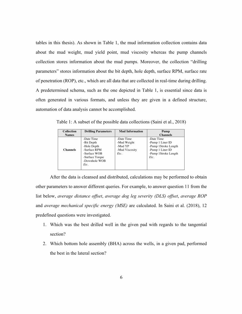
tables in this thesis). As shown in Table 1, the mud information collection contains data
about the mud weight, mud yield point, mud viscosity whereas the pump channels
collection stores information about the mud pumps. Moreover, the collection “drilling
parameters” stores information about the bit depth, hole depth, surface RPM, surface rate
of penetration (ROP), etc., which are all data that are collected in real-time during drilling.
A predetermined schema, such as the one depicted in Table 1, is essential since data is
often generated in various formats, and unless they are given in a defined structure,
automation of data analysis cannot be accomplished.
Table 1: A subset of the possible data collections (Saini et al., 2018)
Collection Names
Drilling Parameters Mud Information Pump Channels
Channels
-Date Time -Bit Depth -Hole Depth -Surface RPM -Surface WOB -Surface Torque -Downhole WOB Etc.
-Date Time -Mud Weight -Mud YP -Mud Viscosity Etc.
-Date Time -Pump 1 Liner ID -Pump 1Stroke Length -Pump 1 Liner ID -Pump 1Stroke Length Etc.
After the data is cleansed and distributed, calculations may be performed to obtain
other parameters to answer different queries. For example, to answer question 11 from the
list below, average distance offset, average dog leg severity (DLS) offset, average ROP
and average mechanical specific energy (MSE) are calculated. In Saini et al. (2018), 12
predefined questions were investigated.
1. Which was the best drilled well in the given pad with regards to the tangential
section?
2. Which bottom hole assembly (BHA) across the wells, in a given pad, performed
the best in the lateral section?

7
3. Which BHA across the wells, in a given pad, performed the best in the vertical
section?
4. Which rig crew performed the best?
5. Which directional driller was the best in a given field?
6. Which BHA had the best directional performance in a given formation?
7. Which BHA had the best drilling performance in a given formation?
8. Which rig crew followed the best connection practices?
9. Which BHA used in the lateral section was the best, from a directional drilling
perspective, at following the planned well path?
10. Which BHA used in the vertical section was the best, from a directional drilling
perspective, at following the planned well path?
11. Which is the best BHA for drilling the initial 1,000 feet of the Lateral Section?
12. Which well’s horizontal section was most efficiently drilled?
In the next section, one of the 12 questions will be used as an example for
demonstrating the storyboarding process.
2.2 IMPLEMENTATION EXAMPLE
The implementation example discussed here uses 16 well dataset from 4 different
drilling pads for question 1: “Which was the best drilled well in the given pad with regards
to the tangential section?”. The data includes raw time-based data, well plan data, survey
files, DDRs, formation tops and BHA data initially obtained as CSV, xlsx and PDF files.
In order to answer the questions, key performance indicators (KPI) need to be calculated.
For instance, the “best well” is defined in three aspects: drilling time, energy transfer
efficiency and wellbore quality each with different KPIs as shown in Table 2. The eight

8
KPIs are then calculated using scripts that use the cleansed data from the collections shown
in Table 1.
Table 2: KPIs for best well (Saini et al., 2018).
Aspects Drilling Time Energy Transfer Efficiency Wellbore Quality
KPIs
1. ROP 2. Depth drilled per unit time
1. Mechanical specific energy (MSE) 2. Ratio of downhole to surface torque 3. Ratio of downhole to surface weight on bit (WOB)
1. Actual versus planned trajectory 2. Tortuosity 3. Vibrations
Table 3: Summary table output for question number one (Saini et al., 2018).
As previously mentioned, the KPIs could be evenly weighted or weighted
depending on the end user’s preference. In this implementation example, the eight KPIs
are evenly weighted. A summary of the calculated KPIs for the top three wells is shown in
Table 3. Only the top three wells are reported, and the remaining 13 wells are excluded
from the storyboard. Amongst the three wells, a rank is assigned to each well for each KPI
after they are compared. The best KPIs will be ranked number 1. Then, a total weighted
rank is summed from the rankings to determine the best well. In other words, the lowest
sum of all rankings will be the best well. In this case, well 1 is the best well among the

9
three wells with the lowest total weighted rank and with the best ranking in all parameters
except depth/time. Several conclusions can be easily drawn directly from Table 3:
• Well 1 has the lowest average vibration with a value of 3.71 (level) followed by
Well 2 and Well 3.
• Well 1 has the fastest average ROP with a value of 164.07 ft/hr followed by Well
3 and Well 2.
After the KPIs are ranked appropriately, a series of visualizations are presented in
a sequence that is based on the weighted KPIs as shown in Table 2. The order of the plots
is important for the users to properly interpret the answer to their question. Plots of KPIs
with higher weights would be shown first, followed by those with lower weights. However,
in this case, the plots are generated in a random order because of the evenly weighted
scenario. A total of 8 plots are created for this question and each plot is discussed
individually in the following section.
• ROP with respect to the well trajectory
• Time from spud to total depth (TD)
• MSE with respect to the well trajectory
• Ratio of downhole to surface torque
• Ratio of downhole to surface WOB
• Actual versus planned trajectories
• Tortuosity
• Vibrations

10
Figure 2: Storyboard Output as a PDF report.
2.2.1 ROP With Well Trajectory
One of the 8 plots, that are generated to answer the question of the user, is the
representation of ROP with respect to the well trajectory, which is shown in Figure 3. From
the graph, the user is able to gain a quick understanding of the ROP change for the 3 wells
with respect to the well trajectory from spud to TD. ROP is colored from low values (red)

11
to high values (green). Moreover, the user is also presented with the average overall ROP
for each well. In this particular case, the visuals do not provide a clear indication of which
well is the best, but the overall average ROPs (with values of 164.07, 146.67 and 154.08
feet/hr for Well 1, Well 2 and Well 3, respectively) indicate Well 1 as the best well
according to this metric.
Figure 3: ROP with well trajectory (Saini et al., 2018).
2.2.2 Hole Depth and Bit Depth versus Time
Another example plot is the representation of hole depth and bit depth versus time
as shown in Figure 4. This plot allows the user to visualize the various drilling operations,
i.e. tripping in/out, on-bottom drilling that occurred for each well. Here, Well 3 had the
shortest total operational time to TD with approximately 150 hours, followed by Well 1
and Well 2, both with approximately 170 hours. Since the total depth for the 3 wells are
similar, Well 3 has the fastest depth per drilling time among them. Therefore, if the user is
interested in improving the operational speed for future operations, it would be useful to

12
use Well 3 as a reference. This plot also provides information about the BHA runs. This
plot also provides information about BHA runs. Well 1 had 3 BHA runs while Well 2 and
Well 3 had 4 BHA runs.
Figure 4: Hole depth and bit depth versus time (Saini et al., 2018).
2.2.3 MSE With Well Trajectory
Figure 5 shows MSE along the well trajectory for the 3 wells with coloring from
lowest MSE (green) to highest MSE (red). MSE is an indicator of the energy needed to
remove a volume of rock. From the 3 graphs, the common trend for MSE along the depth
is low MSE in the shallow section of the trajectory to higher MSE in the middle section
and ending with a highest MSE. From the graph for Well 2, MSE is higher in the middle
section of the well for a longer duration than for the other 2 wells. Moreover, Well 1 has
the lowest MSE overall by 25%. If the formations drilled are assumed to be the same, then
this indicates that Well 1 was drilled with less dysfunction than the other 2 wells. This was
also supported in the previous section where Well 1 only had 3 BHA runs whereas the

13
other 2 wells had 4 BHA runs, indicating that there were probably fewer tool failures in
Well 1.
Figure 5: MSE with well trajectory (Saini et al., 2018).
2.2.4 Downhole to Surface Torque Ratio
In Figure 6, the plots show the ratio of downhole torque to surface torque. The
objective of this KPI is to visualize the efficiency of torque transmission from the surface
along the entire drillstring to the bit. Moreover, it also provides an indirect indication of
the tortuosity and the friction along the well. According to this KPI plots, Well 1 has the
best overall performance according to this KPI, while Well 2 and Well 3 exhibit a lower
ratio just before they reach TD (i.e. less efficient torque transfer).

14
Figure 6: Downhole to surface torque ratio (Saini et al., 2018).
2.2.5 Downhole to Surface WOB Ratio
In Figure 7, the plots show the ratio of downhole WOB to surface WOB. The
purpose of this KPI is to identify the well with the most efficient surface to downhole WOB
transfer. Also, it could serve as an indicator for tortuosity and friction, similar to the
previous KPI. However, in this KPI analysis, there is no significant difference among the
3 wells because all wells exhibit a ratio close to 50%. Note that the number shows that
about half of the WOB applied at surface does not get transferred to the bit, and that thereby
surface WOB is a poor indicator of the actual WOB applied at the bit. This could be an
important piece of information when attempting to optimize drilling performance.

15
Figure 7: Downhole to surface WOB ratio (Saini et al., 2018).
2.2.6 Planned Versus Actual Trajectory
Figure 8 compares the planned trajectory (blue) to the actual trajectory (red) for
each well. The user can use this information to determine directional drilling performance
for each well. For all 3 wells, the actual trajectory is followed along the planned trajectory
from surface through to the first kick off point (KOP) and onward to the tangential section.
However, at the second KOP, the actual trajectory starts to significantly diverge from the
planned trajectory significantly for all 3 wells. This KPI gives the user a quick overview
of the trajectory and may provide a useful reference for drilling new wells on the same pad
while attempting to improve directional drilling performance and well placement. Here,
Well 3 appears to exhibit the worst performance with the largest offset value.

16
Figure 8: Planned and actual trajectory (Saini et al., 2018).
2.2.7 Accrued Tortuosity Index with Measured Depth
Figure 9 plots the accrued tortuosity index (TI) for each well along the measured
depth. A well with a lower TI value is generally considered to have a better wellbore quality.
In this example, Well 1 has the lowest accrued TI with a value of 1.8 compared to Well 2
and Well 3 that have significantly higher values of 4.9 and 7.3, respectively. The purpose
of this KPI is to give the user a quick understanding of the wellbore quality of the wells.

17
Figure 9: Accrued TI with MD (Saini et al., 2018).
2.2.8 Vibration with Actual Trajectory
Lastly, Figure 10 shows a representation of the vibration levels experienced during
drilling, ranging from low vibration (green) to high vibration (red) along the actual
trajectory. Well 1 has more blue and green intervals with only a few yellow and red
intervals compared to the other 2 wells. Therefore, Well 1 has the best overall vibration
performance. The average vibration level is also shown for reference.

18
Figure 10: Vibration with actual trajectory (Saini et al., 2018).
2.3 WORKING WITH NON-PREDEFINED QUESTIONS
The storyboarding concept was initially built around the 12 predefined questions
identified in the previous section. However, the future goal is to be more encompassing by
having a general system which can provide a storyboard for any question of interest to the
user, rather than only addressing a limited number of predefined questions.. This section
introduces 2 methods that could be used to map an arbitrary user question to questions that
are already programmed into the database. As an example, a set of 10 predefined questions
listed below will be used to match the target question: “What is the best well drilled in
West Texas?”.
1. What is the best drilled well in the region/pad?
2. What is the best BHA for the vertical section of the well?
3. Did adding a particular component in the BHA improve performance?
4. Which well has the best wellbore quality?
5. Which rig followed the best connection practice?

19
6. How well did the directional driller do?
7. Which drilling crew performed the best?
8. Which well had the least NPT?
9. How can we improve on the best well?
10. Which is a cost efficient well?
2.3.1 Word Vectorizer
The first method to address the above problem involves using a word vectorizer
module, such as the “TfidfVectorizer” from a Python scikit-learn package. This method
transforms strings of text into vectors and calculates the cosine similarity between 2 texts
using the term frequency–inverse document frequency (tf-idf).
For example, let’s assume that the target question is “What is the best well drilled
in the West Texas?”. First, the target question and the 10 predefined questions are imported
into the Python package. Then, set the vector df to 1 and the vect.fit_transform function in
the package is used to vectorize all the input text strings. Lastly, the vector between target
question and each predefined question is compared. The results from this approach indicate
that question one: “What is the best drilled well in the region/pad?” is the best match to the
target question.
2.3.1 Fuzzy String Matching in Python
The second method uses a Python module called “fuzz” from the Python package
“fuzzywuzzy”. The module compares 2 different text strings and assigns a score ranging
from 0 to 100 for each combination. The combination with the highest score is considered
as the best match.

20
There are various functions: “fuzz.ratio”, “fuzz.partial_ratio”,
“fuzz.token_sort_ratio” and “fuzz.token_set_point” in this module that can be used to
determine the scoring matrix. The appropriate function must be determined under careful
considerations since the output depends on the complexity of the text strings that are
compared.
• If 2 strings are highly similar to each other and are in the correct order, the first
function “fuzz.ratio” should be used for the scoring.
• If the string is out-of-order or partially similar such as “Texas Rangers” and
“Rangers”, then the functions “partial_ratio” or “fuzz.token_sort_ratio” should be
used.
• If the input string exhibits high complexity, then it is suggested that the last function
“fuzz.token_set_point” be used.
In this case, since the target questions could be formed in many different ways, the
function “fuzz.token_set_point” was most applicable to determine the scoring between the
target question and the predetermined question. The highest score for the target question
was 81 out of 100, and corresponds to the predefined question “What is the best drilled
well in a pad/region?”.
Figure 11: Scoring results using FuzzyWuzzy.

21
2.4 CHAPTER SUMMARY
The application of storyboarding to the oil and gas industry was discussed in this
Chapter. Visualizations allow computer-generated answers to questions to be better
received by the end user.. The framework developed provides a foundation for data analysis
automation. A methodology whereby the process could be adapted for different questions
from the end user was also discussed. This process can be facilitated and enhanced by using
spider bots, which will be discussed in the next Chapter.

22
Chapter 3: Spider Bots
3.1 BACKGROUND
Spider bots, typically known as web crawlers, continuously scour the web to gather
information and improve web indexing. Well-known bots such as Googlebot, bingbot,
Yahoo Slurp, etc. also monitor user search results to further improve search quality.
Commonly, spider bots follow a combination of 4 policies: selection, re-visit, politeness
and parallelization.
First, the selection policy targets the selection of websites that the web crawler will
cover. Gulli and Signorini (2005) showed that large-scale web search engines cover only
around 40-70% of the websites. Various selection methods were introduced by Cho (1998)
and Najork and Wiener (2001) to enhance web selection for specific purposes.
Next, the re-visit policy defines the optimal schedule for the web crawler to “re-
crawl” the website that was covered before. A re-visit policy is necessary because websites
are constantly updated, deleted or altered. Cho and Garcia-Molina (2000) defined the re-
visit policy by freshness and age. The objective of the re-visit policy is to keep the local
files as fresh as possible and minimize the age of the local files.
Then, the web crawler must follow the politeness policy of each website. The
politeness policy explains the visiting rate of web crawler to a certain site. This policy must
be followed to ensure the server does not overload and that other web crawlers have the
same opportunity to fetch data from the site.
Lastly, the parallelization policy determines the multi-processing of the web
crawlers to maximize downloading rate while avoiding the re-downloading of the same
data.

23
The 4 policies work together to create a better search quality for the user. In this
thesis, 3 spider bot types or policies, i.e. cleansing, processing and indexing, are introduced
for enhancing the user experience of generating information from raw data.
3.2 SPIDER BOTS IN OIL AND GAS
The idea of spider bots and its application to the oil and gas sector was introduced
by Saini et al. (2018). Spider bots support the storyboarding concept discussed in the
previous Chapter and work to both enhance the quality of reports and reduce the time it
takes to generate a report. Three classes of spider bots are considered: cleansing bots,
processing bots and indexing bots. These 3 bots work together and periodically run in the
background to refresh data and the collections that need to be indexed. The functions and
interaction of the 3 bots are discussed in following sections.
3.2.1 Cleansing Bots
Often, raw drilling data is of poor quality and reliability, and is not well organized.
Since operators collect drilling data from various sources and store them in different
databases, the data could also be in different formats. For example, real-time rig sensor
data is typically stored in historians and often distributed for analysis in the form of CSV
files, whereas DDRs that contains information about non-productive time (NPT), well
control incidents, tripping/drilling data, etc., are manually inputted by rig personnel and
are often distributed as PDF files (as shown in Figure 12) or as CSV files (but formatted in
a variety of ways). Errors often occur in the form of incorrect timestamps, inconsistent
units, missing data points, etc. The objective of the cleansing bots is to identify and remove
the errors and to structure the data into a fixed internal format for faster processing by the
processing bots.

24
Figure 12: Example of BHA information in PDF format.
The cleansing bots are executed under 2 main conditions: 1) new data needs to be
added to the storyboarding database, and 2) new cleansing algorithms are continuously
being developed. The first condition is relatively simple and straightforward. When new
data is entered into the storyboarding database, the cleansing bots are run to perform data
cleansing on the raw data. If the data is already clean and organized, then this step could
be skipped. The second condition is important to the user since the cleansing algorithm
may themselves undergo improvements. In this case, the user might want to re-run the
newly developed cleansing bots on the entire database.
3.2.1.1 Data Cleansing Function and Input/Output Collections
For this project, the cleansing bots are written in Python in the form of a function
called “data_cleansing”. It takes all the raw data and executes cleansing algorithms on the
input collections. The inputs for this function is the complete set of raw data collections,
and the outputs are the cleansed data in cleansed data collections (see Figure 13). Raw data
may be classified into various categories: real-time data, drill string/casing information,

25
well plan information, formation information, drilling mud information, and pump
information.
Figure 13: Input and output collections for data_cleansing function
The output collections are categorized in the same way as the input raw data
collections.
3.2.2 Processing Bots
After the raw data is cleansed and organized, the processing bots will perform
various calculations on the cleansed data in the collections. The calculations are conducted

26
to ensure that at the very least the 12 questions presented in the Chapter 2 can be answered.
For example, to plot the trajectory graph shown in Figure 3, Figure 5 and Figure 8 in the
earlier Chapter, 4 additional parameters require calculation: Northing, Easting, true vertical
depth (TVD) and dogleg severity (DLS). These parameters are calculated from measured
depth (MD), inclination (j1, j2), azimuth (q1, q2) and ratio factor (RF) using the equations
from the Minimum-Curvature Method (MCM) (Mitchell, 2011) listed in Section 3.2.2.2.
The processing bots are executed under 4 conditions: 1) new cleansed data is added
to the database, 2) new processed data that is an input to any of the processing bots is
generated, 3) new algorithms are developed or changes are made to previous processing
algorithms, and 4) new concept or questions are added to the storyboarding process. After
executing the processing bots, the newly created fields and results will be added as new
collections to the database. For the first and second condition, when newly cleansed data
or processed data is added to the database, the processing bots will automatically retrieve
the information needed and perform relevant calculations. For the third condition, new
processing algorithms might be developed using different equations or more efficient
Python scripts. Lastly, new KPIs may be required when new questions are defined for the
storyboarding process. This may also necessitate performing additional calculations on
data in the database.
The processing bots developed for this thesis are contained in nine Python functions:
“cal_MSE”, “minimum_curvature”, “trajectory_offset”, “time_to_depth”,
“parameter_BHA”, “parameter_formation”, “parameter_moving_means”,
“parameter_survey_interval” and “parameter_overall”. Each function will generate
processed collection(s) and these are discussed in more detail in the following sections.
The processing bots not only take cleansed data as input for the calculations but also other

27
processed data as well. In either case, the output collection will only be classified as a
processed collection.
3.2.2.1 MSE Calculation Function and Input/Output Collections
The inputs for the “cal_MSE” Python function are the cleansed “real-time data” and
“BHA information” collections. The purpose of this function is to calculate surface and
downhole MSE. The input parameters are WOB, ROP, bit area, differential pressure, mud
motor speed to flow ratio (rev/gal), motor differential pressure and motor maximum torque.
The output collection is “drilling performance” which contains surface MSE and downhole
MSE.
Figure 14: Input and output collections for cal_MSE function.

28
Surface MSE and downhole MSE values are calculated using the following
equations. Surface MSE is calculated using surface rotation rate (N), surface torque (T),
WOB, ROP and AB, where AB is the bit area (Teale, 1965). Downhole MSE is calculated
using WOB, ROP, AB, surface rotation rate (N), differential pressure (DP), motor
maximum torque (Tmotor,max), motor differential pressure (DPmotor,max), mud motor speed to
flow ratio (K, rev/gal) and flow rate through mud motor (Q) (Logan, 2015).
𝑀𝑆𝐸$%&'()* =𝑊𝑂𝐵𝐴0
+120×𝜋×𝑁×𝑇𝐴0×𝑅𝑂𝑃
(3.1)
𝑀𝑆𝐸;<=>?<@* =
𝑊𝑂𝐵𝐴0
+120×𝜋×(𝑁 + 𝐾×𝑄)×
𝑇E<F<&,E(H∆𝑃E<F<&,E(H
×∆𝑃
𝐴0×𝑅𝑂𝑃
(3.2)
3.2.2.2 Minimum Curvature Function and Input/Output Collections
The inputs for “minimum_curvature” Python function are the cleansed “well plan
information” and “actual survey” collections. The purpose of this function is to calculate
the well trajectory with both the well plan and the survey data. The inputs needed are
inclination, depth and azimuth for both the well plan and the actual survey information
collections. The outputs are MD, inclination, azimuth, DLS, Easting and Northing. The
output collections are called “planned survey” and “final survey”.

29
Figure 15: Input and output collections for minimum_curvature function.
The function uses equations from the Minimum-Curvature method (Mitchell, 2011)
to calculate the parameters for plotting the planned and actual well trajectories shown in
Figure 3, Figure 5 and Figure 8. In the Minimum-Curvature Method, MD, j1, j2, q1, q2 are
knowns and Northing, Easting, TVD, RF and DLS are unknowns. A schematic diagram
for the unknowns and knowns are shown in Figure 16.
𝑁𝑜𝑟𝑡ℎ𝑖𝑛𝑔 = 𝑀𝐷2 × sin𝜑W× cos 𝜃W + sin𝜑[× cos 𝜃[ ×𝑅𝐹 (3.3)
𝐸𝑎𝑠𝑡𝑖𝑛𝑔 = 𝑀𝐷2 × sin𝜑W× sin 𝜃W + sin𝜑[× sin 𝜃[ ×𝑅𝐹 (3.4)
𝑇𝑉𝐷 = 𝑀𝐷2 × cos𝜑W + cos𝜑[ ×𝑅𝐹 (3.5)
𝐷𝐿𝑆 = cosaW[cos(𝜑[ − 𝜑W) − sin𝜑W × sin𝜑[ × 1 − cos(𝜃[ − 𝜃W )] (3.6)

30
𝑅𝐹 =2𝐷𝐿𝑆× tan
𝐷𝐿𝑆2 (3.7)
Figure 16: Schematic diagram of Minimum-Curvature Method (MCM). Mitchell and Miska (2011).
3.2.2.3 Trajectory Offset Function and Input/Output Collections
The purpose of the “trajectory_offset” function is to calculate the distance between
the planned trajectory and actual trajectory. It is intended to evaluate if the well was drilled
according to the planned trajectory or not. The input collections are the processed
collections “planned survey” and “actual survey” generated in section 3.2.2.2. The output
collection is called “trajectory offset” and contains the following fields: hole depth,
distance offset and difference in DLS information.

31
Figure 17: Input and output collections for trajectory_offset function.
3.2.2.4 Time to Depth Function and Input/Output Collection
The purpose of “time_to_depth” function is to transform time-series data to depth
based data. The input collections are the cleansed collection “real-time data” and processed
collection “drilling performance”. The output collection is “Depth Data” with 10 fields.
This function outputs 7 parameters of interest (excluding date time, depth drilled and
drilling duration): differential pressure, RPM, torque, WOB, ROP, surface MSE and
downhole MSE. This function, however, is not limited to these 7 parameters. If the user is
interested in other parameters, the user can input their parameter of interest and obtain
similar results.

32
Figure 18: Input and output collections for time_to_depth function.
3.2.2.5 Parameter BHA Function and Input/Output Collections
The purpose of the “parameter_BHA” function is to calculate the parameters
relevant to BHA performance. For example, the function will calculate the min, max, mean
and standard deviation of parameters such as ROP, RPM, Torque, etc. for each BHA. There
are 4 input collections for this function: “real-time data”, “drilling performance”, “BHA
information” and “mud information”. The output collections are: “parameter BHA Max”,
“parameter BHA min”, “parameter BHA Mean” and “parameter BHA standard deviation”.
From the input collections, only some fields are taken into consideration for the calculation.

33
Figure 19: Input and output collections for parameter_BHA function.
This function processes statistical information for the parameters for faster indexing
and retrieval. It reduces the need to do calculations when the query is made, as the BHA-
based information is already calculated and stored in the database. In this case, 9 parameters
(excluding hole depth): downhole MSE, surface MSE, ROP, RPM, torque, WOB,
differential pressure, mud viscosity and mud yield point were given as inputs to the
function. However, it is not limited to only these 9 parameters. The user can enter any
parameter of interest and obtain similar results.

34
3.2.2.6 Parameter Formation Function and Input/Output Collections
The purpose of the “parameter_formation” is to calculate the parameters on a
formation basis. For example, the function will calculate the min, max, mean and standard
deviation of parameters such as ROP, RPM, Torque, etc. for each geological formation.
There are 4 input collections for this function: “real-time data”, “formation tops”, “mud
information” and “drilling performance”. The output collections are: “parameter formation
Max”, “parameter formation min”, “parameter formation Mean” and “parameter formation
standard deviation”. From the input collections, only some fields are taken into
consideration for the calculation.
Figure 20: Input and output collections for parameter_formation function.

35
The purpose of this function is to calculate statistical information on a formation
basis for faster indexing and retrieval. It reduces the need to do calculations when the query
is made, as the formation-based information is already calculated and stored in the database.
In this case, 10 parameters (excluding hole depth): downhole MSE, surface MSE, ROP,
RPM, torque, WOB, differential pressure, mud weight, mud viscosity and mud yield point
are entered into the function. However, the function is not limited to these inputs. The user
can add additional parameter of interest to the function and receive similar results.
3.2.2.7 Parameter Moving Means Function and Input/Output Collections
The purpose of the “parameter_moving_means” function is to calculate the
parameter’s moving mean. There are 2 input collections for this function: “real-time data”
and “drilling performance”. The output collection is: “parameter moving means”.
There are various methods to calculate moving mean, such as simple moving
average (SMA), cumulative moving average (CMA), weighted moving average (WMA),
exponentially weighted moving average (EWMA). In this function, SMA method is used
to calculate moving means for each parameter. The equation for SMA method is given by:
𝑀𝐴> =𝑃g>
ghW
𝑛 (3.8)
where n is the number of data points in the moving mean average, and P is the
parameter whose moving mean is calculated.

36
Figure 21: Input and output collections for parameter_moving_means function.
3.2.2.8 Parameter Survey Interval Function and Input/Output Collections
The purpose of the “parameter_survey_interval” function is to calculate the
parameter statistics on a survey interval basis. There are 3 input collections for this function:
“real-time data”, “drilling performance” and “final survey”. The output collections are:
“survey parameter max”, “survey parameter min”, “survey parameter mean” and “survey
parameter standard deviation”. In this function, tortuosity index is also calculated; however,
only one value is calculated for each new survey data point and is saved in the “survey
parameter mean” collection.

37
Figure 22: Input and output collections for parameter_survey_interval function.
This function is similar to the functions from section 3.2.2.5 and 3.2.2.6 which
process statistical information for the parameters for faster indexing and retrieval. The
function calculates statistical information on a survey interval basis and stores the
information in the database. In this case, 3 parameters of interest: downhole MSE, surface
MSE and RPM were given as input to the function. However, it is not limited to only these
3 parameters. The user can enter additional parameters of interest and retrieve similar
results.

38
3.2.2.9 Parameter Overall Function and Input/Output Collections
The purpose of the “parameter_overall” function is to calculate the parameter
overall mean and standard deviation for the entire well. For example, the function will
calculate overall mean rate of penetration (ROP) for wells 1, 2, 3, etc. There are 5 input
collections for this function: “real-time data”, “mud information”, “drilling performance”,
“trajectory offset” and “parameter survey mean”. Where the first 2 are cleansed collections,
the last 3 are processed collections. The output collections are: “parameter overall stats”
and “parameter overall standard deviation”.
Figure 23: Input and output collections for parameter_overall function.

39
The goal of this function is to summarize representative values for each well, such
that comparisons between wells can be made easily upon query. Moreover, preprocessing
these summaries allow the user to retrieve results within seconds. Here, there are 13 output
fields (excluding hole depth) for this function; however, the user can add additional
parameters of interest into the function.
3.2.3 Indexing Bots
In order to answer questions such as those presented in the previous Chapter in as
little time as possible, retrieving processed information as quickly as possible is important.
Here, the indexing bots come into play. The purpose of the indexing bots is to make
comparisons between the various parameters, and to store the rankings of these parameters
in a collection for quick future retrieval.
The indexing bots are run under 3 conditions: 1) new data is added to the database,
2) new questions are defined, and 3) updates are made to the indexing algorithms. After
the processing bots perform their calculations, the indexing bots will scour the database to
obtain the information needed to make comparisons and assign rankings. In the first
condition, when new processed data is added to the database, indexing bots will
automatically re-rank the parameters taking the new data into account. For example, a live
well will continue to produce more data as the well progresses. This new data is appended
to the previous data. Per policy, the cleansing bots will now output newly cleansed data,
and the processing bots will adjust calculations accordingly. Ultimately, the indexing bots
will re-rank the parameters based on the new calculations. In the second condition, new
KPIs may need to be defined when new questions are considered. For that reason, new
comparisons must be made based on the KPIs added to accommodate new questions. As

40
for the last condition, the indexing bots are run over the entire database whenever there is
an update to the indexing bot algorithm.
3.2.3.1 Data Indexing Function and Input/Output Collections
The purpose of this function is to compare all the wells in the database for each
parameter and to assign rankings for each parameter. Additionally, overall rankings for the
wells may also be generated. The input collections for this function are “well 1 parameter
overall stats”, “well 2 parameter overall stats”, etc. The number of input collections are
dependent on the number of wells in the database. If there are 5 wells in the database, there
will be 5 input collections. The output collection is “top ranked wells” with 11 fields:
“Name”, “Mean ROP”, “Mean surface MSE”, “Mean difference in DLS”, “Mean tortuosity
index”, “ROP rank”, “Surface MSE rank”, “Difference in DLS rank”, “Tortuosity index
rank”, “Well index” and “Well rank”.
The rankings are given to each well after comparing all the wells in the database.
The wells are ranked according to the parameter’s value, from the highest to the lowest,
and is given a ranking from low to high; for example, ROP, MSE, RPM, torque, WOB. On
the other hand, some parameters such as difference in DLS and Tortuosity Index are ranked
according to the parameters’ value from the lowest to the highest, and are given a ranking
from low to high..
In this work, only 4 parameters, i.e. ROP, surface MSE, difference in DLS and
tortuosity index, were taken into account for comparison. Nevertheless, the function is not
limited to only these 4 parameters.

41
Figure 24: Input and output collections for data_indexing function.
The overall well rank is stored in the well index fields. Each well’s well index is
the accumulation of the rankings for each parameter. The equation for calculating well
index is given in Eq.(3.9). The well with lowest well index is assigned the lowest rank.
𝑊𝑒𝑙𝑙𝐼𝑛𝑑𝑒𝑥 = (𝑅𝑎𝑛𝑘g
o
g
∗ 𝑊𝑒𝑖𝑔ℎ𝑡𝑠g) (3.9)
The well index calculation in this function is of great use when assigning ranking
for all wells in the database. Weighting can be adjusted for each parameter for customized
ranking.

42
3.3 CHAPTER SUMMARY
Figure 25 provides a system view of all the spider bots developed in this work. The
various collections that are generated from each bots are also shown in this figure. The 3
types of spider bots are able to efficiently perform data cleansing, processing and indexing
operations on the drilling dataset. In total, there are 8 raw collections, 8 cleansed collections,
20 processed collections and 1 index collection for each well. This approach is able to
considerably reduce the time to answering relevant performance questions for a well
dataset.
Figure 25: Workflow for the cleansing, processing and indexing bots.

43
Chapter 4: Database Architecture
4.1 BACKGROUND
Cleansing, processing and indexing the data using spider bots involve a lot of
pulling and pushing of the data into a database. There are many relational (SQL) and non-
relational (noSQL) databases available for use. Common relational (SQL) databases such
as MySQL, PostgreSQL, Teradata, etc. have a long history of usage and wide range of
resources. On the other hand, non-relational (noSQL) databases such as Cassandra and
MongoDB are gaining popularity, and are equally applicable for this kind of problem. Both
types of databases have their advantages and disadvantages. In this thesis, MongoDB is
chosen for the database to store data because of the listed reasons:
• MongoDB is free and open source with well documented manuals published online.
• Basic and advanced tutorials courses e.g. database set up, using query language,
schema designs, the use of a Python package named PyMongo, etc. are offered by
MongoDB at no cost.
• A non-relational (noSQL) database provides a flexible schema design option.
• It allows nested fields for each key-pair value for more schema flexibility.
• Different schemas can be stored in the same collection.
4.2 MONGODB
This section will introduce the terminologies used in MongoDB and explain some
of the logic for the schema used to store the data. Figure 26 summarizes the typical
architecture of a MongoDB database. The hierarchy in a MongoDB typically consists of:
1) databases, 2) collections and 3) documents.

44
Figure 26: MongoDB database architecture for database, collection and document (Saini et al., 2018).
A single document is comparable to a single row in a CSV or excel file with header
and associated values. MongoDB stores documents in a JSON format with key-pair value.
In this case, the key would be as listed below, and the value would be the numerical number
following each key. These set of key-pair values together constitute a single document.
• _id
• MD (ftKB)
• Incl
• Azm
• DLS
• Easting

45
• Northing
• TVD
• Sliding percent
• Downhole MSE mean
• ROP mean
• Rotating percent
• Surface MSE mean
• Tortuosity Index
Additionally, another layer of key-pair value can be nested in any key-pair value as
shown in Figure 27. This allows for great flexibility of storing drilling data. The nested
key-pair value comes in handy, especially when storing BHA information.
Figure 27: Example of nested fields schema in MongDB.

46
In this example, the document contains information about the BHA, including BHA
number, start date, end date, bit diameter, bit length, depth in/out, total flow area, bit nozzle
size, revolutions per gallon, differential pressure, maximum torque and drillstring
components. Within the drillstring components field, there are 7 nested fields that describe
the characteristics of the drillstring under consideration, such as item description, type,
joints, length (ft), OD (in), ID (in) and mass/length (lb/ft). This nested JSON feature
increases the flexibility in storing complicated BHA data.
A collection typically consists of one or more documents. The collection in Figure
26, is named “Well 1 Survey Parameters Mean Values”. The collections describe in the
thesis are designed in such a way that relevant information is all stored in the same
collection for faster processing. While this does mean replication of data, it allows for a
better user experience, since all data that need to be shown to the end user is available from
a fewer subset of collections. For example, the collection “Well 1 Survey Parameters Mean
Values”, contains parameters such as MD, TVD, inclination, azimuth, DLS, Easting and
Northing (which are all survey related) but also parameters such as ROP mean, Surface
MSE mean, etc. (which have nothing to do with survey). This collection was generated
such that the data required to plot Figure 3 and Figure 5 is all in one place. It greatly reduces
the time the code takes to fetch data.
Lastly, a database consists of one or multiple collections. In this case, the database
contains 37 collections for each well. There is a total of 8 raw data collections, 8 cleansed
data collections, 20 processed data collections and 1 summary index collection for all the
wells in the database. The database itself can be named by a variety of naming conventions
that would indicate the data stored in the database.

47
Figure 28: 36 collections for each well excluding the index collection (Well 1 as an example).

48
4.3 CHAPTER SUMMARY
This chapter discussed the rationale for choosing MongoDB as the database for this
project. MongoDB provides great flexibility for analyzing drilling datasets. Also, the
schema design and its rationale are explained.

49
Chapter 5: Conclusions and Future Work
5.1 RESULTS
The previous 3 chapters discussed the storyboarding concept, spider bots algorithm
and the MongoDB database architecture. In this chapter, the integration of the 3 concepts
will be presented using an example dataset which consists of 5 wells drilled on a pad. The
workflow integration is shown in Figure 29.
To test the workflow, the method is first applied on 4 wells and tested with a
question. Then, the data for the fifth well is added to the database and the same question is
asked again. The question used in the test is “What is best well drilled?”.
First, the raw data is stored in the MongoDB database. In this case, the raw data
collections start with the names: “Well 1 Raw”, “Well 2 Raw”, “Well 3 Raw” and “Well 4
Raw”. Each well has 8 raw collections as shown in Figure 29. As a result, there is a total
of 32 input collections for the 4 wells.
Next, the cleansing bots pick up data from these 32 collections and perform data
cleansing operations. This includes removing timestamp errors, accounting for missing
data points and ensuring correct units for the data. After the cleansing process is done on
the raw data, the outputs are stored in 32 cleansed collections and are saved in the
MongoDB database for future processing.

50
Figure 29: Workflow for spider bots, MongoDB database and storyboarding.
Then, the processing bots collect the information needed from the cleansed or other
processed collections to perform various calculations, such as time-series to depth-based

51
data transformation, well survey trajectory calculation, tortuosity index calculation, etc.
There is a total of 9 processing functions: “cal_MSE”, “minimum_curvature”,
“trajectory_offset”, “time_to_depth”, “parameter_BHA”, “parameter_formation”,
“parameter_moving_means”, “parameter_survey_interval” and “parameter_overall”
which have been previously discussed in this thesis. This step ensures that all KPIs that are
needed for comparisons are computed. This results in 20 processed collections for each
well.
In the last step, the indexing bots retrieve information from the processed
collections and make comparisons for 4 parameters: ROP, MSE, difference in DLS (actual
vs. planned) and tortuosity index. Then, rankings are assigned to the 4 parameters for the
4 wells in the database. Well index is calculated for the best well with even weights using
Eq. (5.1). This information is stored in the “Top Ranked Wells” collection.
𝑊𝑒𝑙𝑙𝐼𝑛𝑑𝑒𝑥 = (𝑅𝑎𝑛𝑘g
o
g
∗ 𝑊𝑒𝑖𝑔ℎ𝑡𝑠g) (5.1)
The storyboarding scripts then generate a report answering the question that was
posed. To verify that the spider bots performed as expected, the fifth well is added to the
database. The fifth well goes through the exact same steps as mentioned before:
• Raw data is categorized into 8 collections with the name starting with “Well 5 Raw”
and saved in the database;
• Data cleansing is performed on raw data and saved into 8 new cleansed collections;
• Data processing on the cleansed data is performed and outputs 20 collections with
processed values.

52
After the 3 steps listed above are completed, the indexing bots collect data from all
5 wells in the database and recalculate the rankings for each well. As a result, Well 5’s
ranking in the Top Ranked Well collection is updated accordingly (Figure 30).
Figure 30: Summary document for Well 5.
Lastly, the storyboarding script will retrieve ranking information from the “Top
Ranked Wells” collection for creating the storyboarding report. In this PDF report, the first
page contains a summary table including ranking information for the 4 parameters as
shown in Table 4 and Figure 30.

53
Table 4: Summary table for “What is the Best Well Drilled?” for 5 wells.
Parameters Well 1 Well 2 Well 3 Well 4 Well 5
Average ROP (ft/hr) 81.952 81.735 79.877 94.414 90.997
ROP Rank 3 4 5 1 2
Average MSE (MPa) 20363.38 26408.77 23464.85 25673.73 36092.71
MSE Rank 5 2 4 3 1
Average Tortuosity Index 8.35 7.81 12.27 11.54 9.56
Tortuosity Index Rank 2 1 5 4 3
Average Difference in DLS -2.13 -2.48 -2.83 -2.61 -2.99
Difference in DLS Rank 1 2 4 3 5
Well Index 11 9 18 11 11
Well Rank 2 1 5 2 2
In this example, because there are 3 wells with the same well index; therefore, the
3 wells have the same well ranking. This well ranking function can be enhanced by using
weighted values for each parameter (see Eq. (5.1)).
This exercise shows that the time to retrieve useful information from large dataset
is greatly reduced with the use of spider bots. Compared to the current practice in the
industry, which might take days, weeks or even months, this process only takes minutes.
The final PDF report was generated within minutes after the raw data is saved in the
MongoDB database.

54
5.2 FUTURE WORK
The application of storyboarding along with spider bot algorithms in the oil and gas
industry can provide a solid foundation for data exploration and analysis. There is
additional work exploiting advanced machine learning methods that can be done to
improve upon what is presented in thesis.
• First, the number of questions that can be answered through this process can be
expanded.
• Second, the use of Natural Language Processing (NLP) methods in the process can
be used to expand the search, allowing the user to search with keywords of interest.
In addition, a search engine for the database could be created (see Figure 31Error!
Reference source not found.). Here, the user can type a set of keywords and expect
search results to be shown in a hierarchical order. Then, the user can click on the
search result and receives a storyboarding report that answers the question or
matches the keywords.
• Finally, unsupervised learning algorithms can be integrated into the methodology
such that broad outlier phenomena can be identified.
Figure 31: Schematic of a NLP-based search engine for drilling in oil and gas industry.

55
Appendix
RAW COLLECTIONS AND FIELD NAMES
CLEANSED COLLECTIONS AND FIELD NAMES

56
PROCESSED COLLECTIONS AND FIELD NAMES

57
INDEX COLLECTION AND FIELD NAMES

58
References
Abusurra, M. S. M. (2017). Using artificial neural networks to predict formation stresses for marcellus shale with data from drilling operations. ProQuest Dissertations & Theses Global.
Baaziz, A. and Quoniam, L. (2014). How to use Big Data technologies to optimize operations in Upstream Petroleum Industry. In 21st World Petroleum Congress. https://doi.org/10.5585/iji
Burton, S. and Matthewson, L. (2015). Targeted construction storyboards in semantic fieldwork. Methodologies in Semantic Fieldwork.
Cho, J., Garcia-Molina, H. and Page L. (1998). Efficient crawling through URL ordering, Computer Networks and ISDN Systems, Volume 30, Issues 1–7, 1998, Pages 161-172, ISSN 0169-7552, https://doi.org/10.1016/S0169-7552(98)00108-1
Cho, J. and Garcia-Molina, H. (2000). The Evolution of the Web and Implications for an Incremental Crawler. The 26th International Conference on Very Large Data Bases (VLDB '00). https://dl.acm.org/citation.cfm?id=671679
Feblowitz, J. (2013, March 5). Analytics in Oil and Gas: The Big Deal About Big Data. Society of Petroleum Engineers. https://doi.org/10.2118/163717-MS
Gulli, A. and Signorini, A. (2005). The indexable web is more than 11.5 billion pages. The 14th international conference on World Wide Web (WWW '05). http://dx.doi.org/10.1145/1062745.1062789
Holt, H. (1956). The Story of Walt Disney.
Logan, W. D. (2015, September 28). Engineered Shale Completions Based On Common Drilling Data. Society of Petroleum Engineers. https://doi.org/10.2118/174839-MS
Mitchell, R. F. and Miska, S. Z. (2011). Fundamentals of Drilling Engineering. MongoDB 4.0 Manual (2018)
Mostofi, M., Rasouli, V. and Mawuli, E. (2011). An Estimation of Rock Strength Using a Drilling Performance Model: A Case Study in Blacktip Field, Australia. Rock Mechanics and Rock Engineering. https://doi.org/10.1007/s00603-011-0142-9
Najork, M. and Wiener, J. L. (2001). Breadth-first crawling yields high-quality pages. The 10th international conference on World Wide Web. https://doi.org/10.1145/371920.371965
Pollock, J., Stoecker-Sylvia, Z., Veedu, V., Panchal, N. and Elshahawi, H. (2018, April 30). Machine Learning for Improved Directional Drilling. Offshore Technology Conference. https://doi.org/10.4043/28633-MS
Russo, P. (2011). Big Data Analytics, TDWI best practices report. The Data Warehousing Institute (TDWI) Research.

59
Saini, G., Chan, H., Ashok, P., van Oort, E., and Isbell, M. R. (2018, March 6). Automated Large Data Processing: A Storyboarding Process to Quickly Extract Knowledge from Large Drilling Datasets. Society of Petroleum Engineers. https://doi.org/10.2118/189605-MS
Saini, G., Chan, H.-C., Ashok, P., van Oort, E., Behounek, M., Thetford, T., & Shahri, M. (2018, August 9). Spider Bots: Database Enhancing and Indexing Scripts to Efficiently Convert Raw Well Data Into Valuable Knowledge. Unconventional Resources Technology Conference. https://doi.org/10.15530/URTEC-2018-2902181
Teale, R. (1965, March). The concept of specific energy in rock drilling. International Journal of Rock Mechanics and Mining Sciences & Geomechanics Abstracts. https://doi.org/10.1016/0148-9062(65)90022-7
Truong, K. N., et al. (2006). Storyboarding: An Empirical Determination of Best Practices and Effective Guidelines. Proceedings of the 6th ACM Conference on Designing Interactive Systems. https://doi.org/10.1145/1142405.1142410
Whitehead, Mark (2004). Animation. Pocket Essentials.
Zhou, Y., Baumgartner, T., Saini, G., Ashok, P., and van Oort, E., The University of Texas at Austin; Isbell, M.R., Hess Corporation; Trichel, D.K., formerly of Hess Corporation. (2017, March 14-16). Future Workforce Education through Big Data Analysis for Drilling Optimization, SPE-184739-MS, SPE/IADC Drilling Conference and Exhibition. https://doi.org/10.2118/184739-MS

60
Vita
Hong-Chih (Tim) Chan attended National Taiwan University and received a
Bachelor of Science degree in Geosciences in 2015. Later, he began his graduate studies at
the University of Texas at Austin where he worked as a Graduate Research Assistant at
The Rig Automation and Performance in Drilling (RAPID).
Permanent email: [email protected]
This dissertation was typed by the author.