Copyright

by

Donald Do Nguyen

2015

The Dissertation Committee for Donald Do Nguyen

certifies that this is the approved version of the following dissertation:

Galois: A System for Parallel Execution of Irregular Algorithms

Committee:

Keshav Pingali, Supervisor

Lorenzo Alvisi

Richard Lethin

David Padua

Emmett Witchel

Galois: A System for Parallel Execution of Irregular Algorithms

by

Donald Do Nguyen, B.S.

Dissertation

Presented to the Faculty of the Graduate School of

The University of Texas at Austin

in Partial Fulfillment

of the Requirements

for the Degree of

Doctor of Philosophy

The University of Texas at Austin

May 2015

To my family

Acknowledgments

The work in this dissertation was supported by National Science Foundation grants CCF

1337281, CCF 1218568, ACI 1216701, and CNS 1064956. I was also supported by a De-

partment of Energy Sandia Fellowship.

Writing a dissertation is largely a solitary task, but this dissertation would not exist

without the support of colleagues, friends and family. Foremost, my adviser, Keshav Pingali

gave me the advice, encouragement and freedom to pursue my ideas. Most importantly,

Keshav taught me how to think about solving problems and pushed me towards addressing

the important questions.

My committee members—Lorenzo Alvisi, Richard Lethin, David Padua and Em-

mett Witchel—gave me thoughtful comments and much needed perspective to help situate

my work in a broader context.

My frequent collaborators, Amber Hassaan and Andrew Lenharth, were a pleasure

to work with and were always receptive to my latest harebrained ideas. I owe special thanks

to Andrew who opened my eyes to the mysteries of performance optimization.

Through the course of graduate school, I made many friends who provided welcome

relief from the days (and nights) at my desk. I’d like to especially thank Yinon Bentor, Ben

and Shannon Delaware, Thomas Finsterbusch, and Andrew Matsuoka. There is nothing

finer than good drinks with good friends.

My greatest thanks goes to my family. My parents, Dieu and Trung worked tirelessly

so that I was free to follow my passions. My brother, Andrew, introduced me to the wonders

v

of science, and the drive for exploration has stayed with me to this day. Of course, a life of

adventure is meant to be shared. For that, I’m eternally grateful to my fiancee, Rose, who

showed me that a head is only as good as the heart that sustains it.

DONALD DO NGUYEN

The University of Texas at Austin

May 2015

vi

Galois: A System for Parallel Execution of Irregular Algorithms

Publication No.

Donald Do Nguyen, Ph.D.

The University of Texas at Austin, 2015

Supervisor: Keshav Pingali

A programming model which allows users to program with high productivity and which

produces high performance executions has been a goal for decades. This dissertation makes

progress towards this elusive goal by describing the design and implementation of the Ga-

lois system, a parallel programming model for shared-memory, multicore machines. Central

to the design is the idea that scheduling of a program can be decoupled from the core compu-

tational operator and data structures. However, efficient programs often require application-

specific scheduling to achieve best performance. To bridge this gap, an extensible and ab-

stract scheduling policy language is proposed, which allows programmers to focus on se-

lecting high-level scheduling policies while delegating the tedious task of implementing the

policy to a scheduler synthesizer and runtime system. Implementations of deterministic and

prioritized scheduling also are described.

vii

An evaluation of a well-studied benchmark suite reveals that factoring programs

into operators, schedulers and data structures can produce significant performance improve-

ments over unfactored approaches. Comparison of the Galois system with existing program-

ming models for graph analytics shows significant performance improvements, often orders

of magnitude more, due to (1) better support for the restrictive programming models of ex-

isting systems and (2) better support for more sophisticated algorithms and scheduling,

which cannot be expressed in other systems.

viii

Contents

Acknowledgments v

Abstract vii

List of Figures xii

Chapter 1 Introduction 1

Chapter 2 A Data-Centric View of Parallelism and Locality 7

2.1 Model Problem: SSSP . . . . . . . . . . . . . . . . . . . . . . . . . . . . 7

2.2 Operator Formulation . . . . . . . . . . . . . . . . . . . . . . . . . . . . . 9

2.2.1 Baseline Execution Model . . . . . . . . . . . . . . . . . . . . . . 12

2.2.2 TAO Analysis . . . . . . . . . . . . . . . . . . . . . . . . . . . . . 15

2.2.3 Analysis of Iterative Fixpoint Algorithms . . . . . . . . . . . . . . 18

2.3 Parallel Algorithms . . . . . . . . . . . . . . . . . . . . . . . . . . . . . . 23

2.3.1 Delaunay Triangulation . . . . . . . . . . . . . . . . . . . . . . . . 23

2.3.2 Delaunay Mesh Refinement . . . . . . . . . . . . . . . . . . . . . 24

2.3.3 Inclusion-Based Points-to Analysis . . . . . . . . . . . . . . . . . 26

2.3.4 Breadth-First Search . . . . . . . . . . . . . . . . . . . . . . . . . 27

2.3.5 Approximate Diameter . . . . . . . . . . . . . . . . . . . . . . . . 28

2.3.6 Betweenness Centrality . . . . . . . . . . . . . . . . . . . . . . . . 29

ix

2.3.7 Connected Components . . . . . . . . . . . . . . . . . . . . . . . 29

2.3.8 Preflow-Push . . . . . . . . . . . . . . . . . . . . . . . . . . . . . 30

2.3.9 PageRank . . . . . . . . . . . . . . . . . . . . . . . . . . . . . . . 31

2.3.10 Support Vector Machines . . . . . . . . . . . . . . . . . . . . . . . 32

2.3.11 Matrix Completion . . . . . . . . . . . . . . . . . . . . . . . . . . 34

Chapter 3 Parallel Programming Models 37

Chapter 4 The Galois System 40

4.1 Principles of High-Performance Parallelism . . . . . . . . . . . . . . . . . 40

4.2 Separation of Concerns . . . . . . . . . . . . . . . . . . . . . . . . . . . . 44

Chapter 5 Parallel Data Structures 48

5.1 Memory Allocation . . . . . . . . . . . . . . . . . . . . . . . . . . . . . . 49

5.2 Exclusive Locking . . . . . . . . . . . . . . . . . . . . . . . . . . . . . . 51

5.3 Diffracted State . . . . . . . . . . . . . . . . . . . . . . . . . . . . . . . . 54

5.4 Approximate Value Stores . . . . . . . . . . . . . . . . . . . . . . . . . . 55

5.5 Sparse Graphs . . . . . . . . . . . . . . . . . . . . . . . . . . . . . . . . . 61

Chapter 6 Scheduling 63

6.1 Scheduler Building Blocks . . . . . . . . . . . . . . . . . . . . . . . . . . 63

6.1.1 Topology-Aware Bag of Tasks . . . . . . . . . . . . . . . . . . . . 64

6.1.2 Topology-Aware Priority Scheduler . . . . . . . . . . . . . . . . . 67

6.2 Compositional Scheduling Policies . . . . . . . . . . . . . . . . . . . . . . 73

6.2.1 Synthesis . . . . . . . . . . . . . . . . . . . . . . . . . . . . . . . 76

6.2.2 Problems with Naive Composition . . . . . . . . . . . . . . . . . . 77

6.2.3 Relaxed Concurrent Semantics . . . . . . . . . . . . . . . . . . . . 81

6.2.4 Workset Composition . . . . . . . . . . . . . . . . . . . . . . . . . 83

6.2.5 Preliminary Implementation and Evaluation . . . . . . . . . . . . . 87

x

6.3 Exploiting Data Locality . . . . . . . . . . . . . . . . . . . . . . . . . . . 97

6.4 Coordinated Scheduling . . . . . . . . . . . . . . . . . . . . . . . . . . . . 100

6.5 Related Work . . . . . . . . . . . . . . . . . . . . . . . . . . . . . . . . . 101

Chapter 7 Deterministic Scheduling 103

7.1 Interference Graph Scheduling . . . . . . . . . . . . . . . . . . . . . . . . 104

7.1.1 Deterministic Interference Graph Scheduling . . . . . . . . . . . . 108

7.1.2 DIG Optimizations . . . . . . . . . . . . . . . . . . . . . . . . . . 110

7.1.3 Evaluation . . . . . . . . . . . . . . . . . . . . . . . . . . . . . . 113

7.2 Refining Interference Graph Scheduling . . . . . . . . . . . . . . . . . . . 130

7.3 Related Work . . . . . . . . . . . . . . . . . . . . . . . . . . . . . . . . . 131

Chapter 8 Comparison with Other Parallel Programming Models 134

8.1 Rewriting Programs to Conform to Scalability Principles . . . . . . . . . . 135

8.1.1 Applying the Disjoint Access Principle . . . . . . . . . . . . . . . 136

8.1.2 Applying the Virtualization Principle . . . . . . . . . . . . . . . . 138

8.1.3 Evaluation . . . . . . . . . . . . . . . . . . . . . . . . . . . . . . 142

8.2 Parallel Programming Models . . . . . . . . . . . . . . . . . . . . . . . . 154

8.2.1 Other Domain Specific Languages in Galois . . . . . . . . . . . . . 155

8.2.2 Evaluation . . . . . . . . . . . . . . . . . . . . . . . . . . . . . . 158

8.3 Related Work . . . . . . . . . . . . . . . . . . . . . . . . . . . . . . . . . 169

Chapter 9 Conclusion 171

Bibliography 173

xi

List of Figures

2.1 Example of SSSP . . . . . . . . . . . . . . . . . . . . . . . . . . . . . . . 8

2.2 Illustration of the operator formulation . . . . . . . . . . . . . . . . . . . . 9

2.3 Example of a cautious operator . . . . . . . . . . . . . . . . . . . . . . . . 13

2.4 TAO analysis of algorithms . . . . . . . . . . . . . . . . . . . . . . . . . . 14

2.5 Example of node elimination . . . . . . . . . . . . . . . . . . . . . . . . . 18

2.6 Pseudocode for Delaunay triangulation . . . . . . . . . . . . . . . . . . . . 24

2.7 Example of Delaunay triangulation . . . . . . . . . . . . . . . . . . . . . . 25

2.8 Pseudocode for Delaunay mesh refinement . . . . . . . . . . . . . . . . . . 26

2.9 Pseudocode for preflow-push . . . . . . . . . . . . . . . . . . . . . . . . . 31

2.10 Bipartite graph of documents and features . . . . . . . . . . . . . . . . . . 32

2.11 Data access patterns for different matrix completion algorithms . . . . . . . 34

4.1 STAMP programming model . . . . . . . . . . . . . . . . . . . . . . . . . 42

4.2 Example Galois program in C++ . . . . . . . . . . . . . . . . . . . . . . . 46

5.1 Example memory hierarchy for a multicore machine . . . . . . . . . . . . 49

5.2 Marking a location with exclusive locking . . . . . . . . . . . . . . . . . . 52

5.3 Using method flags to indicate desired support for transactional execution . 53

5.4 Execution time of different barrier implementations . . . . . . . . . . . . . 54

5.5 Convergence of SVM-SGD on small input . . . . . . . . . . . . . . . . . . 58

xii

5.6 Speedup of SVM-SGD . . . . . . . . . . . . . . . . . . . . . . . . . . . . 59

5.7 Convergence of GLMNET on large input . . . . . . . . . . . . . . . . . . 60

5.8 Illustration of inlining graph data . . . . . . . . . . . . . . . . . . . . . . . 61

6.1 Organization of distributed chunked LIFO and obim schedulers . . . . . . . 64

6.2 Pseudocode for distributed chunked LIFO . . . . . . . . . . . . . . . . . . 65

6.3 Pseudocode for obim . . . . . . . . . . . . . . . . . . . . . . . . . . . . . 69

6.4 Auxiliary functions for Figure 6.3 . . . . . . . . . . . . . . . . . . . . . . 70

6.5 Scaling of obim and its variants for SSSP application . . . . . . . . . . . . 74

6.6 Scheduling specification syntax . . . . . . . . . . . . . . . . . . . . . . . . 76

6.7 Scheduling rule semantics . . . . . . . . . . . . . . . . . . . . . . . . . . 77

6.8 Application-specific scheduling specifications . . . . . . . . . . . . . . . . 78

6.9 Naive bucketed scheduler . . . . . . . . . . . . . . . . . . . . . . . . . . . 79

6.10 Relationship between M1, M and M2 in the proof of Theorem 6.2 . . . . . 86

6.11 Concrete syntax of HL order (AS1) scheduling policy for PFP application . 88

6.12 Concrete syntax of Global:G1 . . . Local:L1 . . . . . . . . . . . . . . . . 88

6.13 Relative performance when varying synthesizer optimizations . . . . . . . 89

6.14 Datasets used in scheduler synthesis evaluation . . . . . . . . . . . . . . . 90

6.15 Runtime of serial applications . . . . . . . . . . . . . . . . . . . . . . . . 92

6.16 Speedup over best serial applications . . . . . . . . . . . . . . . . . . . . . 93

6.17 Relative number of committed to total iterations for DMR . . . . . . . . . . 94

6.18 Relative number of committed to total iterations for DT . . . . . . . . . . . 95

6.19 Relative number of committed iterations to serial version for PFP . . . . . . 96

6.20 Throughput of matrix completion operators . . . . . . . . . . . . . . . . . 98

6.21 Convergence of matrix completion . . . . . . . . . . . . . . . . . . . . . . 99

7.1 Deterministic scheduler . . . . . . . . . . . . . . . . . . . . . . . . . . . . 106

7.2 Auxiliary functions for deterministic scheduler . . . . . . . . . . . . . . . 107

xiii

7.3 Abort ratio and task execution rates . . . . . . . . . . . . . . . . . . . . . 117

7.4 Atomic updates by application . . . . . . . . . . . . . . . . . . . . . . . . 118

7.5 Speedup with and without CoreDet system on non-deterministic programs . 120

7.6 Speedup of selected deterministic and non-deterministic variants . . . . . . 122

7.7 Baseline times for speedup calculations in deterministic evaluation . . . . . 123

7.8 Performance of variants relative to PBBS . . . . . . . . . . . . . . . . . . 125

7.9 Performance without continuation optimization . . . . . . . . . . . . . . . 126

7.10 DRAM performance . . . . . . . . . . . . . . . . . . . . . . . . . . . . . 127

7.11 Predicted efficiency across applications, variants and thread counts . . . . . 129

7.12 Effect of reordering input . . . . . . . . . . . . . . . . . . . . . . . . . . . 130

8.1 Original STAMP data structures and their scalable alternatives . . . . . . . 137

8.2 Example of converting fine-grain transactions into loop-based ones . . . . . 140

8.3 Scheduling virtualized transactions . . . . . . . . . . . . . . . . . . . . . . 141

8.4 Comparison of Stampede and STAMP programs . . . . . . . . . . . . . . . 143

8.5 Speedup of Stampede over STAMP sequential baseline . . . . . . . . . . . 144

8.6 Speedup of STAMP and Stampede programs with STM and HTM . . . . . 146

8.7 Commit ratios . . . . . . . . . . . . . . . . . . . . . . . . . . . . . . . . . 148

8.8 Performance of STAMP programs with scalable malloc . . . . . . . . . . . 151

8.9 Performance of STAMP programs with XTM . . . . . . . . . . . . . . . . 152

8.10 Approximate lines of code for each DSL feature . . . . . . . . . . . . . . . 156

8.11 Summary of application differences . . . . . . . . . . . . . . . . . . . . . 158

8.12 Input characteristics . . . . . . . . . . . . . . . . . . . . . . . . . . . . . . 160

8.13 Ratio of Ligra and PowerGraph runtimes to Galois . . . . . . . . . . . . . 161

8.14 Ratio of Ligra and PowerGraph runtimes to Ligra-g and PowerGraph-g . . 162

8.15 Runtime for DSLs and Galois with 40 threads . . . . . . . . . . . . . . . . 163

8.16 Approximate diameters computed . . . . . . . . . . . . . . . . . . . . . . 164

8.17 Runtime of PowerGraph on distributed system . . . . . . . . . . . . . . . . 165

xiv

8.18 Runtime for DSLs and Galois with 8 threads . . . . . . . . . . . . . . . . . 166

8.19 Runtime of out-of-core DSLs . . . . . . . . . . . . . . . . . . . . . . . . . 168

xv

Chapter 1

Introduction

Computing devices play a central role in society. With the rise of data centers, which

accounted for 2% of domestic energy consumption in 2012 (Natural Resources Defence

Council, 2014), and the ubiquity of mobile devices, there is increasing need to improve

the efficiency of computation to reduce energy consumption. The best way to improve effi-

ciency is to exploit parallelism and to minimize data movement.

This dissertation addresses performance through the lens of programming models;

it investigates what software program abstractions lead to high performance programs. One

traditional and successful model for programmer productivity is thinking of a program as an

algorithm over data structures or, in the words of Niklaus Wirth, Program = Algorithm +

Data Structure (Wirth, 1978). This model improves productivity because it divides writing

a program into two parts: algorithms that are specific to the problem at hand, and data

structures that are more general and can be reused among different programs.

This dissertation argues that parallel programs require a more refined model. The al-

gorithm itself should be divided into parts, Algorithm = Operator+Schedule. The operator

is the core computation that is specific to a problem, and the schedule is how the computa-

tion is mapped to particular hardware resources in time. In the same way data structures are

reused among sequential programs, schedulers should be reused among parallel programs.

1

Given a decomposition of a program into activities or tasks, the scheduling problem

is the assignment of these activities to processors, and the specification of an order in which

each processor should execute the activities assigned to it. Scheduling is important for both

sequential and parallel implementations of algorithms since it may affect locality and load

balance; it may even effect the total amount of work performed by some programs, as will

be shown shortly.

Scheduling can be done either statically by a compiler or dynamically by a runtime

or operating system. Static scheduling can be used when dependences between activities

are known statically and the execution time of each activity can be estimated accurately

at compile-time. Stencil computations are the classic examples of algorithms amenable to

static scheduling (for example see (Stock et al., 2014)). Dynamic scheduling is useful for

problems in which (1) dependences between activities cannot be elucidated statically, or (2)

new work is created dynamically so the number of activities is not known statically, or (3)

accurate estimates of the time required to execute each activity are not available. The vast

majority of algorithms, including almost all irregular algorithms (algorithms where the key

data structures are sparse graphs) require dynamic scheduling.

For the most part, prior work on dynamic scheduling has focused on problems in

which there are no dependences between activities, and new work is not created dynam-

ically, so the only problem is that the time required to execute an activity cannot be de-

termined accurately. Self-scheduling of DO-ALL loops in OpenMP is the classic example.

Activities in this case correspond to iterations of the DO-ALL loop; the number of iterations

is known before the loop is executed, and it is assumed that there are no dependences be-

tween iterations. However, different iterations may take different and unpredictable amounts

of time to execute, so to ensure good load balance, OpenMP provides scheduling policies

such as chunked dynamic self-scheduling, in which a processor gets a chunk of k iterations

every time it needs work, and guided self-scheduling, in which the chunk size decreases

steadily as the loop nears completion (Dagum and Menon, 1998). Chunking reduces the

2

overheads of scheduling and may improve locality.

More recently, attention has shifted to task-parallelism in which new activities are

created dynamically, although it is still assumed that all activities are independent except

for fork-join control dependences. In OpenMP 3.0, there is support for different dynamic

scheduling policies such as breadth-first and work-first policies (Duran et al., 2008). An-

other popular technique is work-stealing. In work-stealing, each thread has a local deque

that contains activities to execute. When a thread’s local deque is empty, it selects the local

deque of another thread, the victim, and tries to steal activities from it. Work-stealing is

parameterized by the order maintained in the local deque (usually LIFO) and how a thread

selects a victim (usually at random). Work-stealing was implemented in MultiLisp (Hal-

stead, 1985) and was later popularized by the Cilk language (Blumofe et al., 1995), where

it is used to implement fork-join parallelism. It is now available in many programming en-

vironments: Intel Threading Building Blocks (TBB) (Reinders, 2007) the Java library (Lea,

2000) and the .Net library (Leijen et al., 2009).

The key assumptions in such work on task-parallelism are that any dependences

between activities are captured by fork-join control dependences and are known statically.

While these assumptions are reasonable for regular (i.e., dense-array) algorithms and divide-

and-conquer algorithms, they do not hold for most irregular graph algorithms because de-

pendences in these algorithms are complex functions of runtime values (e.g., the shape of

the graph and the values on nodes and edges), which may themselves change during execu-

tion.

An abstract description of parallelism in irregular algorithms is the following. At

each step of the algorithm, there are certain active nodes in the graph where computation

needs to be performed. Performing the computation at an active node may require reading

or writing other graph nodes and edges, known collectively as the neighborhood of that

activity. The neighborhood is usually distinct from the neighbors of the active node. In

general, there are many active nodes in a graph, so a sequential implementation must pick

3

one of them and perform the appropriate computation.

In unordered algorithms, which are the focus of this dissertation, the implementa-

tion is allowed to pick any active node for execution. In contrast, ordered algorithms have a

specific order in which active nodes must be executed. For unordered algorithms, the final

output may be different for different orders of executing active nodes, but all such outputs

are acceptable, a feature known as don’t-care non-determinism. A parallel implementation

of such an algorithm can process active nodes simultaneously, provided their neighborhoods

do not overlap. This condition can be relaxed but is sufficient for correct execution. In gen-

eral, the neighborhood of an activity is not known until the activity has finished execution.

The parallelism that results from processing activities in parallel subject to neigh-

borhood and ordering constraints is amorphous data-parallelism (ADP) (Pingali et al.,

2011). Efficient exploitation of amorphous data-parallelism requires far more sophisticated

runtime support than fork-join parallelism or DO-ALL parallelism for the following rea-

sons.

1. In most irregular algorithms, nodes become active dynamically, so the number of

activities is not known statically.

2. In general, the neighborhood of an activity may be known only after the activity

completes execution. Therefore, it may be necessary to use optimistic or speculative

parallelization.

3. Most importantly, the number of activities that are executed by an algorithm may be

different for different schedules. In some cases, the amount of work may differ by an

asymptotic factor, as shown in the following chapter. If this is the case, it is critical to

capture the scheduling of the more work-efficient scheduling.

For these reasons, even sequential implementations of irregular algorithms often use

handcrafted, algorithm-specific scheduling policies; for example, some mesh refinement al-

gorithms process triangles or tetrahedra in decreasing size order since this can reduce the

4

total amount of refinement work (Miller, 2004). Section 2.3 gives examples of the poli-

cies used in the literature. However, following these orders strictly can dramatically reduce

parallelism, so parallel implementations of irregular algorithms often use more complex

scheduling policies that trade off extra work for increased parallelism. These schedulers are

themselves concurrent data structures and add to the complexity of parallel programming.

In addition, they cannot easily be reused for other applications.

This dissertation introduces a flexible and efficient approach for specifying and syn-

thesizing schedulers for sequential and parallel implementations of irregular algorithms. It

distinguishes between scheduling policies, which are informal descriptions of the order in

which activities should be processed (e.g., LIFO, FIFO, etc.), scheduling specifications,

which are formal descriptions of scheduling policies, and schedulers, which are concrete

implementations of scheduling specifications. A schedule is a specific mapping of activities

to processors in time.

Of course, to address performance, efficient scheduling must be combined with

scalable data structures. The main contribution of this dissertation is the design and imple-

mentation of a parallel programming model for unordered algorithms based on an extensi-

ble scheduling policy DSL and a library of parallel data structures. This system is called the

Galois system.

Chapter 2 describes the core program abstraction in Galois, the operator formu-

lation, and it also shows how the operator formulation is a natural abstraction for many

algorithms. Chapter 3 summarizes existing programming models for parallelism. Chap-

ter 4 introduces the design principles that guide the implementation of the Galois system.

Chapter 5 and Chapter 6 describe the implementation concretely in terms of data struc-

tures and scheduling, respectively. To address one concern with unordered algorithms, their

non-determinism, Chapter 7 presents a deterministic scheduling algorithm that permits un-

ordered algorithms to be run non-deterministically or deterministically as desired.

To support the utility of the Galois system, Chapter 8 evaluates the Galois system

5

in two ways. First, it shows that the design principles introduced in Chapter 4 are suffi-

cient conditions for scalability by showing that their manual application can substantially

improve the performance of the STAMP benchmark suite, a well-studied but until now

poorly performing benchmark suite. Second, Chapter 8 shows that the Galois system is a

significant improvement over existing parallel programming models because (1) existing

programming models can be reimplemented in Galois and obtain better performance than

their original implementations and (2) the Galois system can express more sophisticated

algorithms beyond the capabilities of previous systems, which result in orders of magnitude

performance improvements for many graph analytics problems.

6

Chapter 2

A Data-Centric View of Parallelism

and Locality

This chapter introduces the operator formulation of programs. Section 2.1 describes a model

problem that illustrates the key ideas, and Section 2.2 generalizes the basic issues in the

model problem to develop the operator formulation. Section 2.3 shows how various algo-

rithms can be expressed with this formulation.

2.1 Model Problem: SSSP

Given a weighted graph G = (V,E,w), where V is the set of nodes, E is the set of edges,

andw is a map from edges to edge weights, the single-source shortest-paths (SSSP) problem

is to compute the distance of the shortest path from a given source node s ∈ V to each node

in the graph. Edge weights can be negative, but it is assumed that there are no negative

weight cycles.

In most SSSP algorithms, each node is given a label that holds the distance of the

shortest known path from the source to that node. This label dist(v) is initialized to 0 for

Portions of this chapter have previously appeared in (Pingali et al., 2011), where the TAO classificationwas originally described.

7

x

y

a

b2

1

2

2

1

1

0

88

88

Figure 2.1: Example of SSSP (edge weights shown in blue)

s and ∞ for all other nodes. The basic SSSP operation is edge relaxation (Cormen et al.,

2009): given an edge (u, v) such that dist(u) +w(u, v) < dist(v), the value of dist(v) is

updated to dist(u) + w(u, v). Each relaxation, therefore, lowers the dist label of a node,

and when no further relaxations can be performed, the resulting node labels are the shortest

distances from the source to the nodes, regardless of the order in which the relaxations

were performed. When relaxations are applied arbitrarily, this algorithm is called chaotic

relaxation (Chazan and Miranker, 1969).

Nevertheless, some relaxation orders may converge faster and are therefore more

work-efficient than others. For example, consider the graph in Figure 2.1. Edges in the

graph where edge relaxation can be performed are shown in red. If edge b is relaxed, it will

create new opportunities for edge relaxation at all the outgoing edges of node y. If those

newly enabled edges are processed before edge a, those edges will be processed again once

edge a is relaxed. However, if edge a is processed before edge b, processing edge b will

not create any new opportunities for edge relaxation, and the total number of relaxation

operations is reduced. Dijkstra’s SSSP algorithm (Dijkstra, 1959) applies edge relaxation

to all the outgoing edges of a node and relaxes each node just once by using the following

strategy: from the set of nodes that have not yet been relaxed, pick one that has the minimal

label.

However, Dijkstra’s algorithm does not have much parallelism due to its reliance

on a centralized priority queue, so some parallel implementations of SSSP use this rule

only as a heuristic for priority scheduling: given a choice between two edges with different

dist labels on their sources, they pick the one with the smaller label, but they may also

8

Figure 2.2: Illustration of the operator formulation

execute some edges out of priority order to exploit parallelism. One such algorithm is delta-

stepping SSSP (Meyer and Sanders, 1998). The price of this additional parallelism is that

some nodes may be relaxed repeatedly. A balance must be struck between controlling the

amount of extra work and exposing parallelism.

2.2 Operator Formulation

To discuss common issues in parallel programs, it is convenient to use the terminology of

the operator formulation (Pingali et al., 2011), a data-centric programming model for ex-

pressing parallelism in regular and irregular algorithms. The basic concepts of the operator

formulation are illustrated in Figure 2.2.

• Active nodes are nodes in the graph where computation must be performed; they are

shown as red dots in Figure 2.2.

• The computation at an active node is called an activity, and it results from the appli-

cation of an operator to the active node. In some algorithms, it is more convenient

to think in terms of active edges rather than active nodes. Without loss of generality,

we will use the term active nodes. The operator is a composition of elementary graph

operations with other arithmetic and logical operations.

Note that graphs themselves are general data structures; any other data structure can

9

be expressed as a graph. An array is a node with ordered neighbors. A pointer-based

data structure is a graph of memory locations with edges corresponding to pointers

to other memory locations.

• The set of graph elements read and written by an activity is its neighborhood. The

neighborhood of the activity at each active node in Figure 2.2 is shown as a “cloud”

surrounding that node. If there are several data structures in an algorithm, neighbor-

hoods may span multiple data structures. In general, neighborhoods are distinct from

the set of immediate neighbors of the active node, and neighborhoods of different ac-

tivities may overlap. In a parallel implementation, the semantics of reads and writes

to such overlapping regions must be specified carefully. The general term for what

happens when two activities cannot proceed in parallel due to their neighborhoods is

a conflict.

The SSSP algorithms described in the previous section can be expressed in the

operator formulation. In chaotic relaxation and Dijkstra’s algorithm, the operator is the

edge relaxation operator. The active edges are edges where edge relaxation can be applied,

and the neighborhood is the active edge and the corresponding endpoints of the edge.

In general, there may be multiple active nodes, so an algorithm must specify which

order of executing active nodes is valid. There are two classes of ordering. In unordered

algorithms, any order of processing active nodes is valid. The chaotic relaxation algorithm

for SSSP is an example of an unordered algorithm. In ordered algorithms, the algorithm has

a specific order in which active nodes are processed. Dijkstra’s algorithm is an example. In

that algorithm, active edges must be processed in priority order.

The operator formulation leads to a natural definition of parallelism.

Definition 2.1. Given a set of active nodes and an ordering on it, amorphous data-parallelism

(ADP) is the parallelism that arises from simultaneously processing active nodes subject to

neighborhood and ordering constraints.

10

Amorphous data-parallelism generalizes many common notions of parallelism. ADP

with no neighborhood or ordering constraints is data parallelism (Hillis and Steele, 1986).

ADP with no neighborhood constraints but where activities are ordered according to fork-

join dependencies is nested data-parallelism (Blelloch, 1992). One can go even further.

Instruction-level parallelism (Hennessy and Patterson, 2003) can be seen as an instance of

ADP where (1) activities are processor instructions, (2) activities are ordered according to

program instruction order, and (3) conflicts only occur when neighborhoods overlap and at

least one activity writes to the overlapping region.

ADP also captures many models of consistency. If (1) conflicts only occur when

neighborhoods overlap and at least one activity writes to the overlapping region and (2)

active nodes can be processed in any order, then ADP generates serializable executions (Pa-

padimitriou, 1986). If conflicts only occur when two activities have overlapping neighbor-

hoods and both activities write to the overlapping region, then executions satisfy snapshot

isolation (Berenson et al., 1995).

The operator formulation and ADP permit an abstract description of algorithms that

highlights similarities between algorithms and parallelization techniques across application

domains. At first glance, the chaotic relaxation algorithm for SSSP and the relabel-to-front

algorithm for maximum flow, described in Section 2.3, seem very different, but it turns out

they share many of the same properties in the operator formulation, and optimizations like

ordered execution with priorities (e.g., Dijkstra’s algorithm) that are used for SSSP also

can be used with the maximum flow problem (e.g., HL ordering (Cherkassy and Goldberg,

1995)).

The next section gives a baseline execution model for programs in the operator

formulation, and Section 2.2.2 and Section 2.2.3 describe two techniques to analyze and

optimize programs based solely on their structure in the operator formulation.

11

2.2.1 Baseline Execution Model

The baseline execution model is speculative execution. Shared data structures like graphs

are stored in shared-memory, and active nodes are processed by some number of threads. A

thread picks an active node from a workset1 and speculatively applies the operator to that

node, making calls to a graph library to perform operations as needed. The neighborhood

of an activity grows incrementally as graph methods touch areas of the graph. To detect

conflicts, the graph maintains logical locks associated with each node or edge of the graph.

These locks are acquired by a thread before it can access that element. Locks are held until

the activity terminates. If a thread acquires a logical lock for writing that has been already

acquired by another thread (for reading or writing), a conflict is reported to the runtime

system, which rolls back one of the conflicting activities. Lock manipulation is performed

entirely by the methods in the graph class. In addition, to support rollback, each graph

method that modifies the graph makes a copy of the data before modification.

If active elements are unordered, the activity commits when the application of the

operator is complete, and all acquired locks are then released. If active elements are or-

dered, active nodes can still be processed in any order, but they must appear to commit in

serial order. This can be implemented using a data structure similar to a reorder buffer in

out-of-order processors. In this case, activities that have been executed out-of-order keep

their locks and are held in a reorder buffer until they reach the head of the buffer or are

aborted. Alternatively, a dependence graph can be used to schedule ordered tasks; although,

whether dependence graph scheduling is possible depends on what the order is and how

tasks behave (Hassaan et al., 2015).

For unordered active elements, transactional memory (Harris and Fraser, 2003; Her-

lihy and Moss, 1993) can be used to accelerate conflict detection and rollback in hardware,

see Section 8.1.

What constitutes a neighborhood conflict can be refined or coarsened. A more re-1Throughout this dissertation, the colloquial term workset is used, although more formally, these objects

behave as bags or multisets because they may contain duplicate items.

12

1 Workset ws (G. nodes ( ) )2 foreach Node p in ws :3 / / Phase 1 : r e a d i n g ne ighborhood4 i n t s = 05 f o r Node n in G. n e i g h b o r s ( p ) :6 s += G. g e t D a t a ( n )7 / / F a i l s a f e p o i n t8 / / Phase 2 : w r i t i n g t o ne ighborhood9 / / e l e m e n t s w r i t t e n t o were read i n Phase 1

10 f o r Node n in G. n e i g h b o r s ( p ) :11 G. g e t D a t a ( n ) += s

Figure 2.3: Example of a cautious operator

fined conflict detection scheme would allow activities to proceed in parallel as long as the

corresponding method calls commute with respect to the logical operations they are imple-

menting (Kulkarni et al., 2011). Accesses in disjoint areas of neighborhoods are presumed

to commute. A more coarse conflict detection scheme would allow activities to proceed

only if their neighborhoods are disjoint. Two activities reading or writing the same graph

element would result in a conflict. This scheme can be implemented with exclusive logical

locks that use a compare-and-set instruction to mark a graph element with the id of the

activity that touches it (see Section 5.2).

This speculative executor is sufficient to execute any program in the operator for-

mulation, but it may be inefficient in practice. For instance, the polyhedral model (Feautrier

and Lengauer, 2011) is a methodology that can optimize and schedule array programs with

affine subscripts at compile time without speculation. One way to address the performance

concerns of the baseline execution model is to identify specific program properties that

make programs amenable to certain analysis or execution strategies and use a specialized

executor instead of the baseline executor for these cases.

As an example, sometimes tasks are cautious (Mendez-Lojo et al., 2010), which

means they read their entire neighborhood before writing to any element of it (see Figure 2.3

for an example). For unordered cautious tasks, conflict detection and correction can be

done using lightweight mechanisms because the synchronization problem reduces to the

13

Algorithms

Topology

ActiveNodes

Operator

Structured

Semi-structured

Unstructured

Location

Ordering

Morph

Local computation

Reader

Topology-driven

Data-driven

Unordered

Ordered

Figure 2.4: TAO analysis of algorithms

well-known dining philosopher’s problem (Chandy and Misra, 1984). Conceptually, each

abstract location can be acquired by an owner. The execution of a task can be divided into

two phases: in the first phase, a task reads locations but does not write to any of them,

acquiring ownership of these locations, and in the second phase, the task writes to some

locations, but it does not write to any location that it did not read in the first phase, because

it is cautious. The point between the first and second phase is called the failsafe point. For

cautious tasks, conflicts are detected in the first phase, and rollback is implemented simply

by releasing ownership of all locations. Once the failsafe point has been crossed, global data

structures can be updated in place without the need for backup copies of modified data.

In this spirit, the following two sections describe methods of classifying programs

with an eye towards identifying properties that are useful for optimized execution. The

first is TAO analysis (Pingali et al., 2011) (see Section 2.2.2), which classifies programs

along three dimensions: topology, active nodes and ordering. The second method focuses

on properties of iterative fixpoint algorithms (see Section 2.2.3).

14

2.2.2 TAO Analysis

TAO analysis (Pingali et al., 2011) is a method for structural analysis of algorithms with re-

spect to their possible parallelizations. It is based on classifying algorithms and data struc-

tures along three dimensions.

1. Topology: graph topologies are classified according to the Kolmogorov complexity

of their descriptions. Highly structured topologies can be described concisely with

a small number of parameters, while unstructured topologies require verbose de-

scriptions. The topology of a graph is an important indicator of the kinds of opti-

mizations available to algorithm implementations; for example, algorithms in which

graphs have highly structured topologies may be more amenable to static analysis

and optimization.

• Structured: an example of a structured topology is a graph consisting of labeled

nodes and no edges. This is isomorphic to a set or multiset; its topology can be

described by a single number, the number of elements in the set or multiset. If

the nodes are totally ordered, the graph is isomorphic to a sequence of stream.

Cliques, i.e., graphs in which every pair of nodes is connected by a labeled

edge, are isomorphic to square dense matrices with row/column numbers com-

ing from the total ordering of the nodes. Their topology is completely specified

by a single number, the number of nodes in the clique.

• Semi-structured: trees are classified as semi-structured topologies. Although

trees have useful structural invariants, there are many trees with the same num-

ber of nodes and edges.

• Unstructured: general graphs fall in this category. Even among general graphs,

some may be considered more structured than others. For instance, graphs whose

nodes can be divided into partitions with a small edgecut versus graphs whose

partitions have a large edgecut value.

15

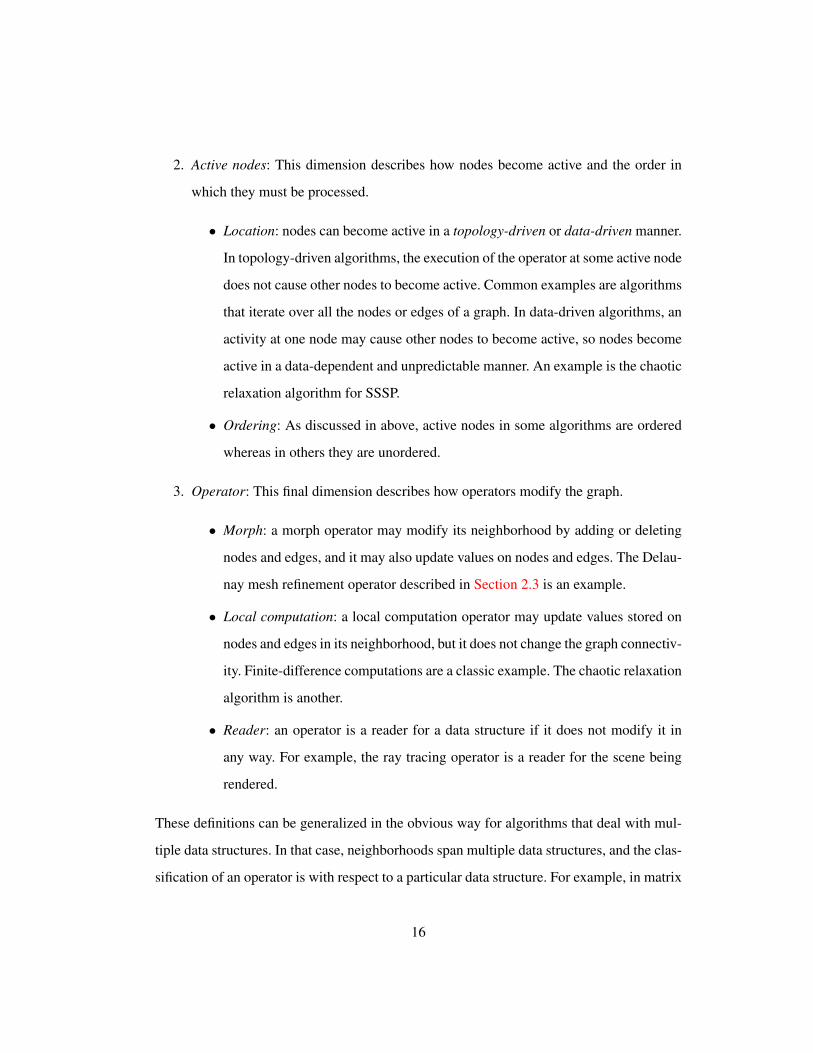
2. Active nodes: This dimension describes how nodes become active and the order in

which they must be processed.

• Location: nodes can become active in a topology-driven or data-driven manner.

In topology-driven algorithms, the execution of the operator at some active node

does not cause other nodes to become active. Common examples are algorithms

that iterate over all the nodes or edges of a graph. In data-driven algorithms, an

activity at one node may cause other nodes to become active, so nodes become

active in a data-dependent and unpredictable manner. An example is the chaotic

relaxation algorithm for SSSP.

• Ordering: As discussed in above, active nodes in some algorithms are ordered

whereas in others they are unordered.

3. Operator: This final dimension describes how operators modify the graph.

• Morph: a morph operator may modify its neighborhood by adding or deleting

nodes and edges, and it may also update values on nodes and edges. The Delau-

nay mesh refinement operator described in Section 2.3 is an example.

• Local computation: a local computation operator may update values stored on

nodes and edges in its neighborhood, but it does not change the graph connectiv-

ity. Finite-difference computations are a classic example. The chaotic relaxation

algorithm is another.

• Reader: an operator is a reader for a data structure if it does not modify it in

any way. For example, the ray tracing operator is a reader for the scene being

rendered.

These definitions can be generalized in the obvious way for algorithms that deal with mul-

tiple data structures. In that case, neighborhoods span multiple data structures, and the clas-

sification of an operator is with respect to a particular data structure. For example, in matrix

16

multiplication, C = AB, the operator is a local computation for C and a reader for matrices

A and B.

TAO analysis can be used to organize programs into classes that share the same

parallelization concerns. For topology-driven active nodes, if the topology and operator are

known at compile-time, which is the case for many dense matrix codes, parallelization can

also occur at compile-time in principle. In practice, to adapt to the variance in the execu-

tion time of tasks, high performance parallelizations of dense matrix codes may also in-

clude a runtime component for load balancing, for instance see the DAGuE system (Bosilca

et al., 2012). A similar trend occurs in data-parallel codes, which also can be parallelized

at compile-time, and often use a work-stealing scheduler (Blumofe et al., 1995) to balance

work among threads at runtime, for instance see (Baskaran et al., 2009).

For sparse matrix codes, the topology (i.e., the structure of the sparse matrix) is

not known until the input is read by the program. Compiler-based parallelization cannot be

used, and the earliest time that parallelization can be attempted is just-in-time, after the input

is read but before the bulk of computation begins. This is called the inspector-executor (Das

et al., 1995) approach. If the matrix is discovered to be relatively dense or if it has dense

subregions (e.g., nearly block-diagonal), the executor in the inspector-executor approach

can apply dense matrix subroutines for parts of the sparse matrix; however, in terms of the

classification of techniques, the earliest point at which the decision to apply these dense

matrix subroutines is when the input is read even though the dense subroutines themselves

may be parallelized at compile-time.

At the most extreme, parallelization may be done at runtime, interleaved with the

parallelized computation itself. This is the case with data-driven active nodes and with

most morph computations. Data-driven active nodes require runtime parallelization because

active nodes are not known without executing the activity.

A similar conclusion holds for morph operators, but one special case is when the

modification performed by the morph can be efficiently simulated without running the op-

17

x

a b

c d

a b

c d

Figure 2.5: Example of node elimination of node x

erator itself. Examples are sparse matrix factorization codes like Cholesky and LU decom-

position. In these codes, the operator performs a morph called node elimination, in which

a node is removed from a graph and edges are inserted as needed between its erstwhile

neighbors to make a clique (see Figure 2.5 for an example). This operator can simulated

by a just-in-time analysis with simple arithmetic operations although the operator itself

requires floating-point operations to compute the factored matrix values. In this applica-

tion area, the simulation of the factorization operator is called symbolic factorization and

is an important step in high-performance, parallel implementations (Gilbert and Schreiber,

1992). Symbolic factorization builds a dependence graph called an elimination tree. The

actual factorization, called numerical factorization, uses the elimination tree to schedule

tasks. LU has an analogous operator, but pivoting is often done to improve numerical sta-

bility. In terms of TAO analysis, the active nodes are data-driven, which means runtime

techniques must be used for parallelization. To facilitate just-in-time parallelization, paral-

lel LU implementations use partial pivoting instead, in which the operator is coarsened to

multiple nodes and pivoting only occurs within a coarsened operator.

TAO analysis is useful for understanding which parallelization strategies are feasi-

ble given a program. The following section describes another type of analysis that explores

possible ways of implementing a particular class of programs, iterative fixpoint algorithms.

2.2.3 Analysis of Iterative Fixpoint Algorithms

Iterative fixpoint algorithms are programs that consist of operators that repeatedly read and

write memory locations until some convergence property is met. A special case of iterative

18

fixpoint algorithms are asynchronous fixpoint algorithms (Bertsekas and Tsitsiklis, 1989).

They are asynchronous because values read may not correspond to the value most recently

written. Asynchronous algorithms2 are amenable to parallel and distributed computation

because they can tolerate long commutation delays. One example of an asynchronous fix-

point algorithm already introduced in this chapter is the chaotic relaxation algorithm for

SSSP.

Iterative algorithms as a class tend to benefit from the same kinds of transforma-

tions. Since some of these transformation change the operator or the asymptotic behavior

of the algorithm, they are not typical optimizations in the compiler community sense of the

term, but nevertheless, they are techniques that application programmers use to improve the

performance of programs.

The foremost transformation is tolerating asynchrony. Whether a program can tol-

erate stale updates is a deep algorithmic property, but once known, parallelizing systems

can exploit this property to restructure communication to follow more efficient patterns at

the machine level. For instance, as originally developed, using stochastic gradient descent

(SGD) for solving linear support vector machines (SVMs) requires reading the most recent

values for the weight vector, but the recently introduced Hogwild approach (Recht et al.,

2011) eschews a serializable locking policy for racy reads and writes. This is possible be-

cause the algorithm tends to still converge even in the presence of noisy or stale data (see

Section 5.4).

The remaining transformations can be summarized as follows: what does the oper-

ator do, where in the graph is it applied, and when is the corresponding activity executed?

What does the operator do? In general, the operator expresses some computation on

the neighborhood elements. In some graph problems such as SSSP, operators can be imple-

mented in two general ways called here push style or pull style. A push-style operator reads2In contrast to asynchronous algorithms which will converge for any communication delay, partially asyn-

chronous algorithms only converge when communication delays are bounded. For the purpose of the discussionin this section, asynchronous and partially asynchronous algorithms are treated interchangeably.

19

the label of the active node and writes to the labels of its neighbors; information flows from

the active node to its neighbors. A push-style SSSP operator attempts to update the dist

label of the immediate neighbors of the active node by performing relaxations with them.

In contrast, a pull-style operator writes to the label of the active node and reads the labels

of its neighbors; information flows to the active node from its neighbors. A pull-style SSSP

operator attempts to update the dist label of the active node by performing relaxations with

each neighbor of the active node. In a parallel implementation, pull-style operators require

less synchronization since there is only one writer per active node.

Usually, the operator represents the smallest logical unit of parallel computation,

but in some cases, the convergence of a fixpoint algorithm can be sped up by coarsening the

graph to speed up the flow of information across the graph. In its simplest form, coarsening

may simply be scheduling multiple activities as one unit or treating subgraphs as a single

node or edge, but the transformations used in practice may also incorporate algorithmic

performance improvements that change the behavior of the operator or the representation

of subgraphs for the coarsened algorithm. The multigrid method for solving linear systems

is a classic example as well as elimination-based dataflow analysis of programs (Allen and

Cocke, 1976). The basic idea is to transform the graph into a smaller subproblem, solve

the subproblem and interpolate the results back onto the original graph. The transforma-

tion, subproblem solving and interpolation steps are application-specific. A related idea is

preconditioning, which is used in iterative linear solvers to preprocess an input to improve

convergence or performance; in this case, the core operation remains the same whether or

not preconditioning is used.

Where is the operator applied? As in TAO analysis, active nodes can be topology-driven

or data-driven.

In a topology-driven computation, active nodes are defined structurally in the graph,

and they are independent of the values on the nodes and edges of the graph. The Bellman-

Ford SSSP algorithm is an example (Bellman, 1958; Ford and Fulkerson, 1962); this al-

20

gorithm performs |V | supersteps, each of which applies a push-style or pull-style operator

to all the edges. Practical implementations terminate the execution if a superstep does not

change the label of any node. Topology-driven computations can be parallelized by parti-

tioning the nodes of the graph between processing elements.

In a data-driven computation, nodes become active in an unpredictable, dynamic

manner based on data values, so active nodes are maintained in a workset. In a data-driven

SSSP program, only the source node is active initially. When the label of a node is updated,

the node is added to the workset if the operator is push-style; for a pull-style operator, the

neighbors of that node are added to the workset. Data-driven implementations can be more

work-efficient than topology-driven ones since work is performed only where it is needed

in the graph. However, load-balancing is more challenging, and careful attention must be

paid to the design of the workset to ensure it does not become a bottleneck.

When is an activity executed? When there are more active nodes than threads, the im-

plementation must decide which active nodes are prioritized for execution and when the

side-effects of the resulting activities become visible to other activities. There are two pop-

ular models that are called here autonomous scheduling and coordinated scheduling.

In autonomous scheduling, activities are executed with transactional semantics, so

their execution appears to be atomic and isolated. Parallel activities are serializable, so

the output of the overall program is the same as some sequential interleaving of activities.

Threads retrieve active nodes from the worklist and execute the corresponding activities,

synchronizing with other threads only as needed to ensure transactional semantics. This

fine-grain synchronization can be implemented using speculative execution with logical

locks or lock-free operations on graph elements. The side-effects of an activity become

visible externally when the activity commits.

Coordinated scheduling, on the other hand, restricts the scheduling of activities to

rounds of execution, as in the Bulk-Synchronous Parallel (BSP) model (Valiant, 1990). The

execution of the entire program is divided into a sequence of supersteps separated by barrier

21

synchronization. In each superstep, a subset of the active nodes is selected and executed.

Writes to shared-memory, in shared-memory implementations, or messages, in distributed-

memory implementations, are considered to be communication from one superstep to the

following superstep. Therefore, each superstep consists of updating memory based on com-

munication from the previous superstep, performing computations, and then issuing com-

munication to the next superstep. Multiple updates to the same location are resolved in

different ways as is done is the varieties of PRAM models, such as by using a reduction

operation (JaJa, 1992).

Application-specific priorities Of the different algorithm classes discussed above, data-

driven, autonomously scheduled algorithms are the most difficult to implement efficiently.

However, they converge much faster than algorithms that use coordinated scheduling for

some problems (Bertsekas and Tsitsiklis, 1989). Moreover, for high-diameter graphs like

road networks, data-driven autonomously scheduled algorithms may be able to exploit more

parallelism than algorithms in other classes; for example, in BFS, if the graph is long and

skinny, the number of nodes at each level will be quite small, limiting parallelism if coordi-

nated scheduling is used.

Autonomously scheduled, data-driven graph analytics algorithms benefit from ap-

plication-specific priorities and priority scheduling to balance work-efficiency and paral-

lelism. One example is delta-stepping SSSP (Meyer and Sanders, 1998), the most com-

monly used parallel implementation of SSSP. The workset of active nodes is implemented,

conceptually, as a sequence of bags, and an active node with label d is mapped to the bag at

position b d∆c, where ∆ is a user-defined parameter. Idle threads pick work from the lowest-

numbered non-empty bag, but active nodes within the same bag may execute in any order

relative to each other. The optimal value of ∆ depends on the graph.

The general picture is the following. Each task t is associated with an integer prior-

ity(t), which is a heuristic measure of the importance of that task for early execution relative

to other tasks. For delta-stepping SSSP, the priority of an SSSP relaxation task is the value

22

b d∆c. A task t1 has earlier priority than a task t2 if priority(t1) < priority(t2). It is

permissible to execute tasks out of priority order, but this may possibly lower work effi-

ciency.3 A good parallel runtime system must permit application programmers to specify

such application and input-specific priorities for tasks, and the system must schedule these

fine-grain tasks with minimal overhead and minimize priority inversions.

2.3 Parallel Algorithms

This section introduces several algorithms using the concepts of the operator formulation,

TAO analysis and analysis of fixpoint algorithms. Pseudocode for these algorithms is writ-

ten using the Galois programming model (see Chapter 4), which is a sequential, object-

oriented programming model augmented with a Galois unordered-set iterator, which is

similar to set iterators in C++ or Java but permits new items to be added to a set while it is

being iterated over.

• foreach T e in S: B(e) — The loop bodyB(e) is executed for each item e of type T

in set S. The order in which iterations execute is indeterminate and can be chosen by

the implementation. There may be dependences between the iterations. An iteration

may add items to S during execution.

2.3.1 Delaunay Triangulation

Finding the Delaunay triangulation (DT) of a set of points is a classic computational geom-

etry problem. There are many algorithms for finding the triangulation; this section describes

the incremental algorithm of Bowyer and Watson (Bowyer, 1981; Watson, 1981). Initially,

there is one large triangle that covers all the points. Then, point p calculates the triangle

that contains it and calculates all triangles whose circumcircles include p. This is the cavity3If the priority order must be strictly followed, the algorithm is ordered and different schedulers must be

applied (Hassaan et al., 2015). This dissertation focuses on implementing unordered algorithms.

23

1 Workset ws ( p o i n t s )2 foreach P o i n t p in ws :3 T r i a n g l e t = f i n d T r i a n g l e C o n t a i n i n g ( p )4 C a v i t y c ( t )5 c . expand ( )6 c . r e t r i a n g u l a t e ( )7 G. u p d a t e ( c )

Figure 2.6: Pseudocode for Delaunay triangulation

of p. Finding the triangle that contains a point can be accomplished with a spatial accel-

eration structure like a kd-tree or oct-tree over triangles. The cavity is re-triangulated, p is

removed, and the next point is processed. This process continues until there are no more

points to process. Figure 2.6 shows the pseudocode. G is the graph representing the trian-

gulation. Figure 2.7 shows an example of processing one point. To reduce the amount of

time spent updating the acceleration structure, it can be built over a subset of triangles and

a geometric search within the mesh can be used to find the enclosing triangle.

All orders of processing points lead to the same Delaunay triangulation. Clark-

son and Shor have shown that selecting points at random is optimal (Clarkson and Shor,

1989). Amenta et al. present an algorithm called biased randomized insertion order (BRIO)

that takes advantage of spatial locality while still maintaining the optimality of random-

ness (Amenta et al., 2003). Briefly, let n be the number of points to triangulate. Points are

processed in log n rounds. The probability that a point is processed in the final round is12 . For the remaining points, the probability that they will be processed in the next-to-last

round is 12 , and so on until the first round. For the first round, all remaining points are pro-

cessed with probability one. Within a round, points are processed according to the spatial

divisions of an oct-tree.

2.3.2 Delaunay Mesh Refinement

Delaunay mesh refinement (DMR) (Chew, 1993) is an algorithm related to Delaunay trian-

gulation. Given a Delaunay triangulation, triangles may have to satisfy additional quality

24

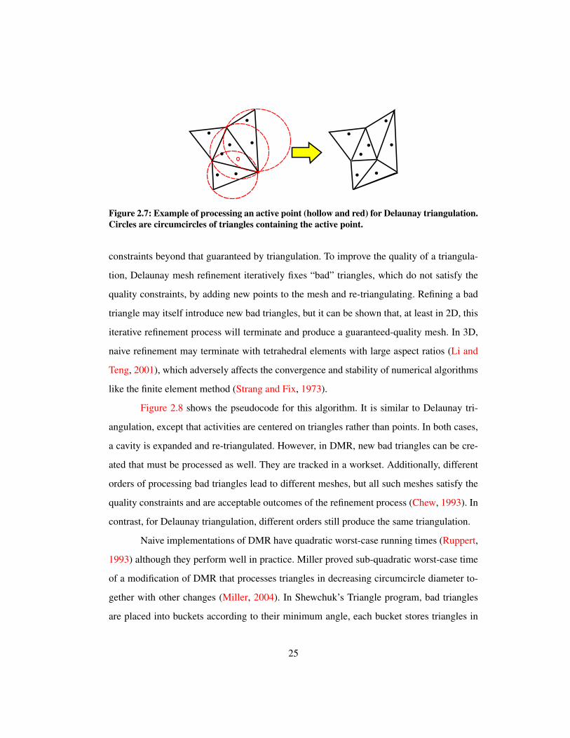
Figure 2.7: Example of processing an active point (hollow and red) for Delaunay triangulation.Circles are circumcircles of triangles containing the active point.

constraints beyond that guaranteed by triangulation. To improve the quality of a triangula-

tion, Delaunay mesh refinement iteratively fixes “bad” triangles, which do not satisfy the

quality constraints, by adding new points to the mesh and re-triangulating. Refining a bad

triangle may itself introduce new bad triangles, but it can be shown that, at least in 2D, this

iterative refinement process will terminate and produce a guaranteed-quality mesh. In 3D,

naive refinement may terminate with tetrahedral elements with large aspect ratios (Li and

Teng, 2001), which adversely affects the convergence and stability of numerical algorithms

like the finite element method (Strang and Fix, 1973).

Figure 2.8 shows the pseudocode for this algorithm. It is similar to Delaunay tri-

angulation, except that activities are centered on triangles rather than points. In both cases,

a cavity is expanded and re-triangulated. However, in DMR, new bad triangles can be cre-

ated that must be processed as well. They are tracked in a workset. Additionally, different

orders of processing bad triangles lead to different meshes, but all such meshes satisfy the

quality constraints and are acceptable outcomes of the refinement process (Chew, 1993). In

contrast, for Delaunay triangulation, different orders still produce the same triangulation.

Naive implementations of DMR have quadratic worst-case running times (Ruppert,

1993) although they perform well in practice. Miller proved sub-quadratic worst-case time

of a modification of DMR that processes triangles in decreasing circumcircle diameter to-

gether with other changes (Miller, 2004). In Shewchuk’s Triangle program, bad triangles

are placed into buckets according to their minimum angle, each bucket stores triangles in

25

1 Workset ws (G. b a d T r i a n g l e s ( ) )2 foreach T r i a n g l e t in ws :3 i f !G. c o n t a i n s ( t ) :4 c o n t in u e5 C a v i t y c ( t )6 c . expand ( )7 c . r e t r i a n g u l a t e ( )8 G. u p d a t e ( c )9 ws . add Al l ( c . b a d T r i a n g l e s ( ) )

Figure 2.8: Pseudocode for Delaunay mesh refinement

FIFO order, and buckets are processed in increasing angle order (Shewchuk, 1996). Kulka-

rni et al. showed that a parallel implementation of DMR that distributes the initial bad tri-

angles among threads and uses thread-local stacks for newly created bad triangles performs

well in practice (Kulkarni et al., 2008).

2.3.3 Inclusion-Based Points-to Analysis

Inclusion-based points-to analysis (PTA), also known as Andersen’s algorithm (Andersen,

1994), is a flow and context-insensitive static analysis that determines the points-to relation

for program variables. PTA is a fixpoint algorithm that computes the least solution to a sys-

tem of set constraints. The basic algorithm maintains a workset of program variables whose

points-to relations need to be computed. For each variable in the workset, the algorithm

examines the system of constraints to see if the current variable satisfies the constraints. If

so, the algorithm continues processing the remaining variables. If not, some set of program

variables are modified to satisfy the constraints. These modified variables are then added

to the workset, and the algorithm continues until the workset is empty. Hardekopf and Lin

showed how the basic fixpoint algorithm augmented with sophisticated cycle detection can

scale to large problem sizes (Hardekopf and Lin, 2007). From this algorithm, Mendez-

Lojo et al. produced the first parallel implementation of this algorithm (Mendez-Lojo et al.,

2010). The results in Section 6.2.5 are based on this implementation.

Since this is a fixpoint algorithm, all orders of processing variables will produce

26

the same solution. Many heuristics have been proposed for organizing the workset, such as

processing variables in least recently fired (LRF) order (Pearce et al., 2003) or dividing the

workset into current and next parts (Nielson et al., 1999). Variables are processed from the

current part, but newly active variables are enqueued onto the next part. When the current

part is empty, the roles of the current and next parts are swapped. Hardekopf and Lin report

that the divided workset approach performs better in practice (Hardekopf and Lin, 2007).

2.3.4 Breadth-First Search

Given an unweighted graph G = (V,E) and a starting node s ∈ V , breadth-first search

(BFS) numbering is the problem of labeling each node with the length of the shortest

path from s to that node. BFS is a special case of the SSSP problem, where all edge

weights are one. Depending on the structure of the graph, there are two important opti-

mizations. For low-diameter graphs, it beneficial to switch between push and pull-based

operators, which reduces the total number of memory accesses (Beamer et al., 2012). For

high-diameter graphs, it is beneficial to use autonomous scheduling. Coordinated execution

with high-diameter graphs produces many rounds with very few activities per round, while

autonomous execution can exploit parallelism among rounds.

BFS algorithms apply the relaxation operator until convergence. For a push-based

operator, the active node is a labeled node, and the operator assigns labels to unlabeled

neighbors of the active node. For a pull-based operator, the active node is an unlabeled

node, and the operator assigns it a label if it can find a labeled neighbor. At the begin-

ning of the computation, it is more efficient to use a push-based operator since there are

few labeled nodes and each edge relaxation propagates information through the graph; con-

versely, it is advantageous to switch to a pull-based implementation towards the end of the

computation when most nodes are labeled, particularly for low-diameter graphs. It is possi-

ble to blend coordinated and autonomous scheduling as well to create a hybrid algorithm.

Initially, the algorithm uses coordinated scheduling of the push and pull-based operators.

27

After a certain number of rounds of push-based traversals, the algorithm switches to pri-

oritized autonomous scheduling with a priority function that favors executing nodes with

smaller BFS numbers.

2.3.5 Approximate Diameter

The diameter of a graph is the maximum length of the shortest paths between all pairs of

nodes. One exact algorithm is to compute all-pairs shortest-paths and return the maximum

distance found. The cost of computing this exactly is prohibitive for any large graph, so

many applications call for an approximation of the diameter (DIA) of a graph.

One algorithm is based on finding pseudo-peripheral nodes in the graph. The eccen-

tricity ecc(v) of a node v is the maximum shortest distance between v and any other node.

A node is pseudo-peripheral if for every node u with distance ecc(v) from v, ecc(u) =

ecc(v). The algorithm begins by computing a BFS from an arbitrary node. Then, it com-

putes another BFS from the node with maximum distance, discovered by the first BFS. In

the case of ties for maximum distance, the algorithm picks a node with the least degree. It

continues this process until the maximum distance does not increase.

Another algorithm is to use the coordinated execution of BFS from k starting nodes

at the same time. The k parameter is often picked such that the search data for a node fits in

a single machine word so that it can be updated using machine atomic instructions. A bit-

vector records whether the node has been visited by a BFS from starting node i < k. Edge

relaxation performs logical-or on bit-vectors. The diameter is estimated by the maximum

distance reached by the k breadth-first searches, which is a lower-bound on the diameter.

Another possibility is to use probabilistic counting (Flajolet and Martin, 1985),

which estimates the number of unique vertex pairs with paths with a distance at most k.

When the estimate converges, k is an estimation of the diameter of the graph.

28

2.3.6 Betweenness Centrality

Given a graph G = (V,E) and a pair of nodes s, t, the betweenness score of a node v is the

fraction of shortest paths between s and t that pass through v. The betweenness centrality

(BC) of v is the sum of all its betweenness scores for all possible pairs s, t in G. A popular

algorithm by Brandes (Brandes, 2001) computes the betweenness centrality of all nodes by

using forward and backward breadth-first graph traversals. There are two major dimensions

of parallelization. One dimension is to compute the scores for multiple source nodes at a

time (outer loop parallelism). This is completely data-parallel. The other dimension is to

parallelize the computation of the scores with respect to a single source node (inner loop

parallelism). Inner loop parallelization can be accomplished by using the same techniques

as breadth-first search (Prountzos and Pingali, 2013).

2.3.7 Connected Components

In an undirected graph, a connected component (CC) is a maximal set of nodes that are

reachable from each other. One algorithm to compute the connected components of a graph

is to iteratively apply BFS, choosing as a starting node any unvisited node in the graph until

there are no more unvisited nodes. This algorithm is O(|V | + |E|) but has a sequential

dependency on the results of previous breadth-first searches. A more parallel algorithm is

based on a concurrent union-find data structure. It is a topology-driven computation where

each edge of the graph is visited once to add it to the union-find data structure. Another

algorithm is based on iterative label propagation. Each node of the graph is initially given a

unique id. Then, each node updates its label to be the minimum value id among itself and its

neighbors. This process continues until no node updates its label, and it will converge slowly

if the diameter of the graph is high. The complexity of this algorithm is O(d(|V | + |E|))

where d is the diameter of the graph.

29

2.3.8 Preflow-Push

Given a directed graph G = (V,E), a capacity function c : E → R+ mapping edges

to non-negative values, and source and sink nodes s, t ∈ V , the preflow-push algorithm

computes the maximal flow from source to sink. Unlike in maxflow algorithms based on

augmenting paths, nodes in preflow-push can temporarily have more flow coming into them

than going out. Each node n maintains its excess inflow excess(n). Each node n also

has a label called height, which is an estimate of the distance from n to t in the residual

graph induced by unsaturated edges. Nodes with non-zero excess that are not the source nor

sink are contained in a workset. These nodes are called active nodes (Goldberg and Tarjan,

1988). The preflow-push algorithm repeatedly selects a node from the workset. Each node

tries to eliminate its excess by pushing flow to a neighbor (see Figure 2.9). Pushing flow

may cause a neighbor to become active. A node can only push flow to a neighbor at a lower

height. If a node is active but no neighbors are eligible to receive flow, the node relabels

itself, increasing its height to one more than its lowest height neighbor.

Cherkassy and Goldberg show the importance of two heuristics named global rela-

beling and gap relabeling (Cherkassy and Goldberg, 1995). Global relabeling is a technique

that periodically reassigns heights by performing a breadth-first traversal from the sink. The

frequency of global relabeling is determined empirically. Gap relabeling is a technique that

preemptively removes from the workset any nodes that cannot push flow to the sink. The

key insight is that if no node has height h, all nodes with height greater than h cannot push

flow to the sink. Cherkassy and Goldberg also consider two orders for processing active

nodes: HL order, where nodes are processed in decreasing height order, and FIFO order.

30

1 Workset ws (s )2 foreach Node u in ws :3 L1 :4 whi le u . e x c e s s > 0 :5 f o r Node v : u . n e i g h b o r s ( ) :6 f l o a t cap = G. edgeData ( u , v )7 i f cap > 0 && u . h e i g h t == v . h e i g h t + 1 :8 pushFlow ( u , v , min ( cap , u . e x c e s s ) )9 i f v != s && v != t :

10 ws . add ( v )11 i f u . e x c e s s == 0 :12 break L113 r e l a b e l ( u )14 i f ∗ :15 g l o b a l R e l a b e l ( )

Figure 2.9: Pseudocode for preflow-push

2.3.9 PageRank

PageRank is an algorithm for computing the importance of nodes in an unweighted graph.

At its core is the following update rule

w(i+1)(v) = α+ (1− α)∑

u∈I(v)

w(i)(u)

|N(u)|

where w(i)(v) is the current PageRank value for v at iteration i, I(v) and N(v) are the

incoming and outgoing neighbors of v respectively, and 0 ≤ α < 1 is some fixed damping

parameter. The update rule is applied until the PageRank values converge.

Algorithms differ in how this update rule is scheduled. Topology-driven algorithms

update all nodes. In the early implementations of the Google search engine, PageRank

was computed using power iteration (Brin and Page, 1998), which is a topology-driven

approach. Data-driven algorithms update only nodes whose neighbors’ PageRank value has

changed significantly. Another data-driven approach is to take samples from the graph (Leskovec

and Faloutsos, 2006). Algorithms also vary in the consistency model used; in some cases,

very weak consistency models have been used, like unsynchronized updates to shared

31

d1

d2

d3

d4

k1

k2

k3

Figure 2.10: Bipartite graph of documents and features

PageRank values (Low et al., 2010). Convergence can vary significantly with scheduling

and consistency model. A possible priority function is to prefer earlier execution of nodes

with the greatest change in value.

The PageRank algorithm can be reduced to a sparse matrix-vector multiply. Instead

of working on the input graph, the algorithm works on the transpose of the graph with

edge weights added corresponding to the number of outgoing neighbors in the original

input graph. That is, given an input graph G and its adjacency matrix representation A,

the algorithm processes a matrix T , such that Tji = Aij · |N(i)|. The topology-driven and

coordinated sweep of the PageRank update above to all the nodes in the graph is equivalent

to the following matrix product, w(i+1) = T w(i).

2.3.10 Support Vector Machines

Given a set of documents, a set of keywords (i.e., the features), and a partial function on

documents indicating whether a document belongs to a class (i.e., binary classification), the

problem is to learn a classifier for all documents. These inputs can be modeled as a bipartite

graph with documents on one side and keywords on the other side; if a keyword k appears

in a document d, there is an undirected edge (d, k) whose weight is the frequency of that

keyword in that document, as shown in Figure 2.10 (weights are not shown in this figure).

One way to solve this problem is to train a support vector machine (SVM). Many

algorithms for SVMs associate a value with each keyword node in the bipartite graph (these

are called the model parameters), and iteratively update these parameters until some conver-

32

gence criterion is met. Stochastic gradient descent (SGD) is particular way of implementing

this idea. An update loop iterates over each document, updating the model parameters at

the immediate neighbors (keywords) of that document; for example, in Figure 2.10, the val-

ues at k1 and k2 are updated when d1 is processed (the value at d1 is read-only). There is

no particular order in which documents need to be visited in each iteration, so this is an

example of an unordered algorithm. An outer loop is used to repeat the update loop until

convergence.

One way to parallelize this algorithm is to recognize that if two documents do not

have keywords in common (such as documents d1 and d4 in Figure 2.10), they can be

processed in parallel. The inspector-executor approach (Das et al., 1995) can be used to

implement this parallelization strategy; given the graph, the inspector finds a conflict-free

schedule. Unfortunately, in realistic data sets, most keywords occur in most documents, so

the bipartite graph is fairly dense and there are usually very few documents that can be

processed in parallel with this parallelization strategy. Similarly, speculative parallelization

will not find much parallelism either.

One way to cut this Gordian knot is to change the semantics of loads and stores to

values at keywords to permit more parallelism in the update loop. The machine learning

community has explored three variations of this theme.

• Local (Agarwal et al., 2014). Documents are partitioned between threads but each

thread has a local copy of values associated with all keywords. Threads update key-

word values independently. Periodically, keyword values from different threads are

merged together using an application-specific merge function.

• Hogwild (Recht et al., 2011). Documents are partitioned between threads and there is

only one copy of keyword values. Threads update keyword values without synchro-

nization, and the cache-coherency protocol in hardware serializes writes to the same

cache line in some order.

• Stale synchronous (Ho et al., 2013). This is a bulk-synchronous strategy. The program

33

u1

u2

u3

u4

i1

i2

i3

(a) Stochasticgradient descent

u1

u2

u3

u4

i1

i2

i3

(b) Coordinatedescent

u1

u2

u3

u4

i1

i2

i3

(c) Alternatingleast squares

Figure 2.11: Data access patterns for the operator in different matrix completion algorithms.Red indicates values being updated. Blue indicates values being read.

is executed in rounds; in each round, threads read keyword values computed in the

last round. Updates to keyword values are accumulated locally to each thread, and at

the end of the round, all updates for a given keyword are merged for use in the next

round.

2.3.11 Matrix Completion

The following matrix completion problem underlies many modern recommender systems.

One is given a partially observed m × n ratings matrix A ∈ Rm×n, where m denotes the

number of users and n the number of items. Let Ω ⊆ 1 . . .m × 1, . . . , n denote the

observed entries of A, i.e., (i, j) ∈ Ω indicates that user i gave item j a rating of Aij . The

goal is to predict accurately the unobserved ratings.

One popular “latent factor” model for matrix completion finds matricesW ∈ Rm×k

and H ∈ Rm×k with k min(m,n) such that A ≈ WH> by minimizing the following

objective function

f(W,H) :=1

2

∑(i,j)∈Ω

(Aij −w>i hj

)2+ λ

(‖wi‖2 + ‖hj‖2

), (2.1)

where wi and hj denote the i-th and j-th row of W and H respectively, and λ is a scalar

parameter.

34

In the operator formulation, the matrix A is considered to be a bipartite graph in

which the nodes consist of either users or items, and an edge with weight Aij indicates that

the i-th user has given a rating ofAij to the j-th item (see Figure 2.11). Three common ways

of solving this matrix completion problem can be expressed with the operator formulation.

Stochastic Gradient Descent (SGD) SGD when applied to Equation 2.1 performs the

following update operations:

wi ← wi − η((

Aij −w>i hj

)hj +

λ

|Ωi|wi

)hj ← hj − η

((Aij −w>i hj

)wi +

λ∣∣Ωj

∣∣hj

)

where η is a scalar step-size, and |Ωi| (resp.∣∣Ωj

∣∣) denotes the number of observed

entries in the i-th row (resp. j-th column) of A. All edges of the graph are the active, and

they can be scheduled in different orders such as cyclic, randomized or prioritized order.

The operator can be applied in parallel to any set of edges which do not share a vertex

in common. For more rapid convergence, a variety of priority functions can be used. For

example, users who have rated a lot of items can be processed before others.

Unlike SGD when applied to the SVM problem, which accesses a document and

all its keywords, the SGD update for matrix completion only needs to access data associ-

ated with an edge and its endpoints. This is because the model parameters for the matrix

completion problem are much sparser than for the SVM problem (i.e., w versus wi,hj).

35

Coordinate Descent (CD) CD will apply the following update operator to every nodewit

of wi and hjt of hj respectively:

wit ←∑

j∈Ωi

((Aij −w>i hj

)+ withjt

)hjt

λ+∑

j∈Ωih2jt

hjt ←∑

i∈Ωj

((Aij −w>i hj

)+ hjtwit

)wit

λ+∑

i∈Ωjw2it

In the most common variant, vertices are cycled through repeatedly. The operator

can be applied in parallel to any set of active nodes and their neighbors as long as they don’t

share a vertex that has to be updated.

Alternating Least Squares (ALS) The ALS operator for w is

wi ←(H>Ωi

HΩi + λI)−1

H>ai

for i = 1, 2, . . . ,m, where HΩi denotes the sub-matrix of H formed by selecting the rows

j ∈ Ωi, and I is the identity matrix, and ai is the i-th row of A. A symmetric update

can be derived for hj . The algorithm repeatedly cycles through the vertices of the graph

and applies the updates. The operator can be applied in parallel to all users but it requires

barrier synchronization after cycling through the users before it can be applied to all the

items.

36

Chapter 3

Parallel Programming Models

Abstractions for parallelism have a rich history. One of the oldest is the dependence graph.

The idea of a dependence or task graph goes back to at least the 1950s when the US Navy

used them for project management (Jarnagin, 1960). Central to a dependence graph is that

dependencies are ordered or directed. Task a depends on task b. This directed representation

appeared in software program abstractions as early as the control flow graph (CFG) (Allen,

1970) in the early 1970s. Around the same time, but independently, the database com-

munity developed systems based on serializability, which is an unordered abstraction for

dependencies. Task a and task b should appear to execute in some order. These models of

computation only began to intersect in the early 1990s with the proposal of transactional

memory (TM) (Herlihy and Moss, 1993), a mechanism designed to provide the database

notion of transactional execution to programs in general, but it would be at least a decade

before practical TM systems became available.

The 1990s also saw sustained interest in auto-parallelization, which is the idea that

a compiler would take a program with sequential semantics and find opportunities for par-

allelization automatically. Prior to this, parallelism was usually expressed explicitly either

through direct use of low-level machine primitives (e.g., vector instructions) or through a

program abstraction like data-parallelism (Hillis and Steele, 1986). Due to the difficulties

37

of producing good parallelizations automatically, the most visible auto-parallelizing sys-

tem, HPF (Kennedy et al., 2007), never gained any traction. Performance of HPF programs

depended on careful data placement. Users annotated data structures with placement poli-

cies, and a compiler generated communication schedules. However, the placement policies

available were drawn from a small set and not extensible.

The mid-2000s saw a new growth (Charles et al., 2005; Allen et al., 2007; Chamber-

lain et al., 2007) of parallel programming models as the DARPA High Productivity Com-

puting Systems project sought ways to achieve high performance with high programmer

productivity. To avoid reliance on the compiler to find parallelism, these new languages re-

quired programmers to indicate parallelism explicitly. The underlying model of parallelism

was generally a fusion of data-parallelism with task dependencies.

As no parallel programming model has become dominant, this expansion of paral-

lel programming models continues to this day with proposals for general (Dean and Ghe-

mawat, 2004; Bauer et al., 2012) and application-specific (Kale and Krishnan, 1993; Low

et al., 2010; Kepner and Gilbert, 2011) models for parallelization. In most parallel program-

ming models, the system takes sole responsibility for scheduling parallel tasks, and there is

one fixed scheduling algorithm that it uses. For instance, Cilk (Blumofe et al., 1995) uses

randomized workstealing with thread-local deques. In systems that do provide a number

of schedulers like OpenMP (Dagum and Menon, 1998), the choices are from a small fixed

menu (e.g., block, block-cyclic). From the discussion in Chapter 2, it is clear that more flex-

ibility in scheduling is needed to cover the diversity of parallel algorithms. For instance, the

different algorithms for SSSP can be seen as the same operator with different scheduling

policies.

If we want a variety of scheduling policies, how should this be accomplished? Since

schedulers are complex pieces of concurrent code, one cannot expect general-purpose pro-

grammers to implement them directly. There should be an intermediate point between im-

plementing schedulers from scratch, which is error-prone, and selecting from a small set of

38

schedulers, which is insufficient for many algorithms.

Additionally, the implementation of the operator and its data structures can be in-

fluenced by which schedules are possible, or in other words, some data consistency models

are more efficient to implement than others. E.g., it is much easier to implement a shared

counter under bulk-synchronous consistency than to implement one under linearizability.

How should these opportunities be exploited when schedules fall in these special cases?

The Galois system, which is described in the following chapters, is one answer to

these questions. To address the need for a variety of schedulers, the Galois system pro-

vides an extensible library of scheduling policies and a scheduler synthesizer to produce a

concurrent scheduler from a high-level specification. To address the implementation of the

operator and its data structures, the Galois system uses exclusive locking for serializable

schedules. For more relaxed consistency models, it uses a methodology called diffracted

state to produce efficient data structure implementations even in the presence of frequent

sharing.

39

Chapter 4

The Galois System

The Galois system is software library and runtime system for parallelizing programs in

shared-memory based on the operator formulation (Section 2.2). Its main goal is the ef-

ficient parallelization of general unordered programs with high programmer productivity

(i.e., a small amount of additional programmer effort). This chapter describes the principles

that underlie the design of the Galois system, and the next two chapters describe how those

principles are put into practice in the implementation of parallel data structures (Chapter 5)

and scheduling (Chapter 6).

The Galois system is designed for shared-memory multicore systems. This means

that there is a single address space of memory and there are multiple threads of execution.

Threads are assigned to cores of a multicore processor, and there may be multiple proces-

sors per machine. Communication between processors may be slower than communication

between cores.

4.1 Principles of High-Performance Parallelism

This section articulates two design principles that must be embodied in scalable parallel

programs. These principles arise from the fact that the most common limiting factor on

40

scalability is data movement. Communication adds costs that increase as the number of

threads or machines increases, so the best way to improve the scalability of a program is to

(1) reduce communication and (2) to be tolerant of communication costs. Concretely, this

means the following for parallel programming models.

Principle 4.1 (Disjoint accesses). Tasks that are disjoint at the logical level should be

disjoint at the physical level.

This principle is a guide for reducing or eliminating conflicts between tasks that

logically should be able to execute concurrently: it says that concurrent tasks should not

conflict if they operate on disjoint data. For example, tasks that add and remove different

items to a bag should not interfere because they operate on disjoint data, even though they

operate on the same data structure. An implementation of a concurrent bag that uses a

single lock, for example, violates this principle. Here and in the remainder of this section,

the term conflict is used in a general sense. A conflict can mean introducing synchronization

to preserve program semantics or it can mean writing to a shared cache line which causes

an invalidation at the cache coherency protocol level.

Principle 4.2 (Virtualized tasks). Tasks should be virtualized.

Tasks are virtualized if their execution is not tied to a particular thread or schedule.

This principle is a guide for ensuring that threads do useful work even in the presence of

conflicts or communication delays. When this happens, implementations have flexibility in

choosing when tasks should execute. For instance, a thread can set aside task and perform

other work instead of waiting for a response for a remote memory request.

These principles may not be surprising, but parallel programs do not necessary

satisfy either principle. Consider the STAMP benchmark suite (Cao Minh et al., 2008), a

widely used suite of programs for evaluating parallel transactional memory (TM) programs,

and to illustrate the key ideas, consider the yada benchmark in STAMP, which performs

Delaunay mesh refinement of a triangular mesh. Figure 4.1 shows a simplified version. A

41

1 Workset wl23 void f unc ( i n t t h r e a d i d ) :4 whi le t rue :5 Task t = atomic wl . pop ( ) 6 i f ! t :7 break8 Tasks newTs = atomic work ( t , t h r e a d i d ) 9 f o r Task n t in newTs :

10 atomic wl . push ( n t ) 1112 t h r e a d r u n ( func , n u m t h r e a d s )

Figure 4.1: STAMP programming model

workset tracks the initial work and work generated during the progression of the algorithm.

Conceptually, each task represents a bad triangle. A workset of bad triangles, implemented

using a linked-list, is populated by walking over the initial mesh and testing each triangle

for badness using simple geometric tests on its vertices.

To process and eliminate a bad triangle, a small neighborhood of triangles surround-

ing the bad triangle is identified (i.e., the cavity) and deleted from the mesh. The region pre-

viously occupied by these triangles is then re-triangulated, and the new triangles are added

to the mesh. Some of these newly created triangles may be bad; if so, they are added to the

workset. In the pseudocode of Figure 4.1, this functionality is implemented by the function

work.

Parallelism in this algorithm arises from the fact that each cavity is usually a small

region of the overall mesh, so bad triangles whose cavities do not overlap can be processed

in parallel. However, it is difficult to tell a priori whether or not the cavities of two bad

triangles will overlap, so static parallelization does not work. Instead, we can consider the

processing of each bad triangle to be a transaction and execute transactions speculatively,

leaving it to the TM system to detect and recover from conflicts on the fly.

In yada, therefore, there are two concurrent data structures: the mesh and the work-

set of bad triangles. In the pseudocode shown in Figure 4.1, each thread executes the func-

42

tion func. The body of this function is a while loop that terminates when the workset is

empty. A thread pops a work-item from the workset using a transaction to synchronize with

other threads that may be manipulating the workset at the same time. The function work

is then called to perform the computation; in yada, this is the processing of the bad trian-

gle, which must be performed transactionally since the mesh is being updated by multiple

threads simultaneously. Finally, any newly created bad triangles are added to the workset

using another transaction.

The programming model and data structures in the STAMP implementation of yada

violate both principles for scalable parallel performance introduced earlier.

Workset push and pop operations from different threads conflict because a linked-

list is used to represent the workset. At the logical level however, two threads that pop work

items from the workset touch different data items, so they should not conflict according to

the disjoint access principle. Similar considerations apply to the representation of the graph

data structure: as long as cavities do not overlap, transactions should not conflict. However,

the graph representation used in STAMP, which uses a linked-list to store nodes, introduces

spurious conflicts, violating the principle of disjoint access.

In addition, the explicitly threaded programming model of Figure 4.1 violates the

principle of virtualized transactions. Once a transaction is attempted by a thread, there is

no way for the thread to put aside that transaction if it aborts and do some other work;

instead, the same thread must keep trying to finish that transaction until it commits. This

limits scheduling freedom and reduces processor utilization.

While this discussion has focused on yada, similar issues arise in the other STAMP

benchmarks. And while STAMP uses transactions to implement synchronization, a more

traditional parallel program using locks and threads would follow a similar structure, and

similar issues arise in parallel programs written by non-performance experts.

So, what can be learned from this example? First, most parallel programming mod-

els focus on scheduling parallelism, but addressing the performance problems in yada re-

43

quire addressing issues with scheduling and data structures. Second, addressing these issues

is not the intended use of TM but solving them is important for performance. Once yada

was modified to conform to the two performance principles, its execution time was reduced

by a factor of 62 on a 32 thread execution (see Section 8.1). Following these principles is

important for improved performance.

Now, rewriting programs by hand to conform the scalability principles introduced

here may be feasible for a small number of performance critical and widely used applica-

tions, but how can these performance insights be applied to the large number of parallel

programs being written today? The solution proposed by this dissertation is a program-

ming model approach where judicious application of abstraction encourages programmers

to write scalable programs.

4.2 Separation of Concerns

The goal of the Galois system is efficient and high-productivity parallelization. Productivity

is achieved through abstraction. Certain information is hidden from the programmer and its

implementation becomes the responsibility of the programming system, while other infor-

mation is made explicit and must be provided by the programmer. When a system requires

very little from the programmer, it promotes high productivity.

High productivity tends to be in tension with high performance. The less informa-

tion given by the programmer, the more a system must infer and the more likely that the

inferred information is suboptimal with respect to performance. Conversely, a dedicated

programmer with a sufficient amount of time can produce a program from scratch that per-

forms as well as or outperforms any one created by a programming system. The scientific

and engineering question becomes choosing where to draw the line between programmer

and system in such a way that balances productivity with performance.

One classic division of labor between programmer and system is the abstract data

type (ADT) (Liskov and Zilles, 1974). Programs are written against interfaces (e.g., list, set,

44

map) that specify a set of methods and their behavior (e.g., list append, list remove), but the

implementation details are hidden, and programmers can interchange different ADT imple-

mentations (i.e., data structures) with, at most, modest program changes. Niklaus Wirth’s

aphorism “Algorithms + Data Structures = Programs” (Wirth, 1978) memorably alludes to

the importance of ADTs to programming.

One reason for the success of ADTs is due to the fact that they factor “what” is done

from “how” it is done. Programmers can focus on solving their problems without getting

bogged down in the details. Another reason for the success of ADTs is due to the fact that

they can grow organically. Language designers cannot select in advance all the components

that programmers will need. ADTs provide a way for programmers to develop components

themselves, as the need arises, without having to leave the programming system.

The common programming abstractions for parallelism—threads, data-parallel loops,

task graph scheduling—do not satisfy these criteria. Threads closely match the underlying

machine semantics, so users must deal with low-level concerns like memory models and

data races. This contravenes the principle of abstraction. Not all parallel programs can be

expressed solely as data-parallel loops or task graphs (Hassaan et al., 2015), so program-

mers must look outside these abstractions to parallelize certain codes. This contravenes the

principle of growth.

The operator formulation offers one solution to this problem by abstracting a paral-

lel task from its implementation and is complete with respect to the applications studied in

this dissertation.

The Galois system is an implementation of the operator formulation for unordered

algorithms within a sequential programming language. Application programmers write par-

allel programs without explicit parallel programming constructs like threads and locks. In

the current system, the sequential language is C++. Key features of the system are the fol-

lowing.

• Application programmers specify parallelism implicitly by using an unordered-set

45

1 G a l o i s : : Graph : : F i r s t G r a p h<Node , Edge> G;23 s t r u c t O p e r a t o r 4 void operator ( ) ( P o i n t p , G a l o i s : : Use rCon tex t<P o i n t>& ws ) 5 T r i a n g l e t = f i n d T r i a n g l e C o n t a i n i n g ( p ) ;6 C a v i t y c ( t ) ;7 c . expand ( ) ;8 c . r e t r i a n g u l a t e ( ) ;9 G. u p d a t e ( c ) ;

10 11 ;1213 void main ( ) 14 s t d : : v e c t o r<P o i n t> p o i n t s = r e a d P o i n t s F r o m F i l e ( ) ;15 G = c o n s t r u c t I n i t i a l G r a p h ( )16 G a l o i s : : f o r e a c h ( p o i n t s . b e g i n ( ) , p o i n t s . end ( ) , O p e r a t o r ( ) ) ;17

Figure 4.2: Example Galois program in C++. This is the concrete implementation of pseu-docode in Figure 2.6.

iterator which iterates over a workset of active nodes. The workset is initialized with

a set of active nodes before the iterator begins execution. The execution of a iteration

can create new active nodes, and these are added to the workset when that iteration

completes execution.

• The body of the iterator is the implementation of the operator, and it is an imperative

action that reads and writes global data structures. Iterations are required to be cau-

tious: an iteration must read all elements in its neighborhood before it writes to any of

them. This is not a significant restriction since the natural way of writing applications

tends to produce cautious iterations.

• The relative order in which iterations are executed is left unspecified in the applica-

tion code; the only requirement is that the final result should be identical to that ob-

tained by executing the iterations sequentially in some order. An optional application-

specific priority order for iterations can be specified (see Section 6.2), and the imple-

mentation tries to respect this order when it schedules iterations.

46

• The system exploits parallelism by executing iterations in parallel. To ensure seri-

alizability of iterations, programmers must use a library of built-in concurrent data

structures for graphs, worksets, etc. (see Chapter 5). These library routines expose

a standard API to programmers, and they implement lightweight synchronization to

ensure serializability of iterations (see Section 5.2).

Figure 4.2 shows an example Galois program in C++ for the pseudocode given in

Figure 2.6. The program is implicitly parallel. Locks and synchronization are performed on

the programmer’s behalf by the data structure and scheduling library. Since data structures

are abstract and synchronization and scheduling are implicit, the Galois system is free to

use scalable implementations without changing the program; compare this model with the

STAMP program described earlier (Figure 4.1). There, important decisions about schedul-

ing and data structure implementations are fixed by the programmer and cannot be changed

without changing the meaning of the program.

47

Chapter 5

Parallel Data Structures

The Galois system is based around a library of data structures and scheduling policies. This

chapter describes the basic data structures used in the Galois system. The main challenge

in implementing data structures is following the disjoint access principle (Principle 4.1).

For example, a red-black tree may be a reasonable implementation of an associative map

for sequential programs, but performing tree operations in parallel requires careful syn-

chronization, and shared accesses on the root of the tree can be a performance bottleneck.

A more scalable implementation is a hashtable, which is a more decentralized alternative,

since logically disjoint operations can be implemented with operations on disjoint memory

areas.

Of course, some data structure operations require communication to implement;

e.g., finding the minimum value in a set in parallel requires some communication between

threads. When communication must be done, Galois data structures try to accomplish it

through the lowest cost communication pathways in the machine. In shared-memory multi-

core machines, memory is organized hierarchically (see Figure 5.1), and the communication

cost between two threads is a decreasing function of the height of their least common ances-

tor in the memory hierarchy, where the height of the root is zero. Communication between

Portions of this chapter have previously appeared in (Nguyen et al., 2013), where the Galois memoryallocator was originally described.

48

Core

Package

...

Thread

NUMA

Host

10 2 3

0 1

0

0

0

Figure 5.1: Example memory hierarchy for a multicore machine

threads that share the same core is faster than communication between threads that only

share the same package, which in turn is faster than communication between threads that

have nothing in common except that they are running on the same machine. Here, communi-

cation refers to reading and writing the same cache line. Large-scale non-uniform memory

access (NUMA) machines may have more levels of hierarchy than shown in the figure, al-

though the general cost pattern remains the same. Thus, when global communication must

be done, the cheapest way to implement it is to use a communication tree that follows the

memory hierarchy. This is similar to how distributed reduction algorithms are implemented.

All Galois data structures are built on top of a scalable memory allocator that is

described in the next section. Section 5.2 describes how Galois data structures implement

transactional execution by using an exclusive locking discipline. Section 5.3 introduces

a methodology called diffracted state for reducing communication costs by following a

machine’s communication hierarchy. Finally, Section 5.4 and Section 5.5 go in depth into

the implementation of two specific data structures, an approximate value store and a sparse

graph.

5.1 Memory Allocation

Galois data structures are based on a custom scalable memory allocator. While there has

been considerable effort towards creating scalable memory allocators (Berger et al., 2000;

Michael, 2004; Schneider et al., 2006), existing general solutions do not scale to large-scale

multi-threaded workloads that are very allocation intensive nor do they directly address non-

49

uniform memory access (NUMA) concerns, which are important for even modestly sized

multi-core architectures. Recently, there has been some effort in designing NUMA-aware

data structures specifically for local computations over graphs (Zhang et al., 2015).

Providing a general, scalable memory allocator is a large undertaking, particularly

because Galois supports morph applications that modify graphs by adding and removing

nodes and edges. For most applications, memory allocation is generally restricted to two

cases: allocations in the runtime (including library data structures) and allocations in an

activity to track per-activity state.

For the first case, the Galois runtime system uses a slab allocator, which allo-

cates memory from pools of fixed-size blocks. This allocator is scalable but cannot handle

variable-sized blocks efficiently due to the overhead of managing fragmentation. The sec-

ond case involves allocations from user code, which may require variable-sized allocation

but also have a defined lifetime, i.e., the duration of an activity. For this case, the Galois

system uses a bump-pointer region allocator.

The slab allocator has a separate allocator for each block size and a central page

pool, which contains huge pages allocated from the operating system. Each thread maintains

a free list of blocks. Blocks are allocated first from the free list. If the list is empty, the thread

acquires a page from the page pool and uses bump-pointer allocation to divide the page into

blocks.

The page pool is NUMA-aware; freed pages are returned to the region of the pool

representing the memory node they were allocated from.

Allocating pages from the operating system can be a significant scalability bottle-

neck (Yoo et al., 2009; Clements et al., 2012), so to initialize the page pool, each application

preallocates some number of pages prior to parallel execution; the exact amount varies by

application.

The bump-pointer allocator manages allocations of per-activity data structures, which

come from temporaries created by user code in the operator. This allocator supports stan-

50

dard C++ allocator semantics, making it usable with all standard containers. The allocator

is backed by a page from the page pool. If the allocation size exceeds the page size (2 MB),

the allocator falls back to malloc.

Each activity executes on a thread, which has its own instance of the bump-pointer

allocator. The allocator is reused (after being reset) between iterations on a thread. Since

the lifetimes of the objects allocated are bound to an activity, all memory can be reclaimed

at once at the end of the activity.

5.2 Exclusive Locking

The Galois system uses exclusive locking to implement transactional execution. This con-

trasts with transactional memory (TM) systems, which ensure transactional execution by

monitoring reads and writes to memory. One challenge tackled by the TM community is

supporting a high amount of concurrency by sometimes allowing a read in one transaction

to proceed in the presence of a concurrent read or write to the same address in another

transaction.

In multicore architectures, writing to a shared cache line is a potential scalabil-

ity bottleneck, and scalable programs are typically written (or rewritten) to not have such

sharing (Clements et al., 2013), e.g., replacing red-black trees with hashtables. Having a

conflict detection scheme that permits activities to write to a shared cache line enables a

level of concurrency at the task level that is not scalable at the cache coherency level.

An alternative is to simply not permit activities to proceed if they access the same

memory locations. One such scheme is exclusive locking. Whenever an activity reads or

writes memory, it marks that location with its activity id. If another activity has already

marked the location, the current activity aborts, rolling back its state changes and clearing

its marks. When a activity finishes, it also clears its marks.

Figure 5.2 shows pseudocode for this mark functionality, which must be called be-

fore reading or writing a memory location. The value−1 is used to indicate that the location

51

1 s t r u c t E x c l u s i v e L o c a t i o n :2 T v a l u e3 T o l d V a l u e4 i n t owner5 E x c l u s i v e L o c a t i o n ∗ n e x t67 ThreadLoca l<i n t> myId8 ThreadLoca l<E x c l u s i v e L o c a t i o n∗> myLocs9

10 void mark ( E x c l u s i v e L o c a t i o n ∗ l ) :11 whi le t rue :12 i f l−>owner == myId :13 re turn14 e l s e i f l−>owner != −1:15 r o l l b a c k ( )16 / / r e t u r n s t o s c h e d u l e r t o r e s c h e d u l e17 r a i s e A b o r t ( )18 e l s e i f compareAndSwap(& l−>owner , −1, myId ) :19 / / i f l−>owner was −1 and i t i s20 / / s u c c e s s f u l l y upda ted t o myId21 l−>o l d V a l u e = l−>v a l u e22 l−>n e x t = myLocs23 myLocs = l24 re turn

Figure 5.2: Marking a location with exclusive locking

has not been marked by any activity. Exclusive locations acquired by an activity are main-

tained in a linked-list. To clear its marks, an activity walks its list of marked locations, sets

the owner fields back to the unacquired value, and resets the next fields to null. Rollback

is similar to clearing marks except that the activity additionally restores the value to the

previously stored old value. One optimization is to use transactional boosting (Herlihy and

Koskinen, 2008) and use undo logs to rollback state. In the Galois system, an activity is as-

sumed to be cautious. That is, it reads all its locations before modifying any of them. In this

case, there is no state to rollback when a conflict occurs because no writes have happened

yet.

Exclusive locking fails fast on activities that other conflict detection schemes would

permit to continue. However, if a program follows the disjoint access and virtualization prin-

ciples, the number of conflicts should be small because (1) activities access mostly disjoint

52

1 s t r u c t Graph :2 / / . . .3 NodeData& g e t D a t a ( GraphNode n , MethodFlag m = ALL ) :4 / / Re tu rn da ta a s s o c i a t e d w i t h graph node n56 Graph g7 GraphNode n89 g . g e t D a t a ( n ) / / Get da ta w i t h f u l l t r a n s a c t i o n a l e x e c u t i o n

10 g . g e t D a t a ( n , NONE) / / Get da ta w i t h o u t t r a n s a c t i o n a l e x e c u t i o n

Figure 5.3: Using method flags to indicate desired support for transactional execution

data and (2) aborted activities can be rescheduled to reduce conflicts. Exclusive locking also

reflects the realities of modern hardware. Writes to shared cache lines are scalability bot-

tlenecks, and exclusive locking reflects the performance model of the underlying hardware

directly in the programming model. This makes potential problems more obvious, which

encourages programmers to address them early.

A useful optimization is to bypass exclusive locking when an operator only per-

forms a simple update to a machine word or when transactional execution is not needed at

all. For these cases, all Galois data structure methods have an optional parameter that indi-

cates whether an operation always or never acquires locks. Experienced users can disable

locking and use machine atomic instructions if desired (see Figure 5.3).

An objection to exclusive locking is that it produces conflicts with read-only work-

loads. Locations that are always read-only can usually be determined statically (e.g., (Lat-

tner et al., 2007)). For situations where a location is sometimes read and sometimes written,

TMs that allow concurrent reads typically use timestamp-based validation (Dice et al., 2006;

Riegel et al., 2006), which has its own scalability cost because a global counter is atomi-

cally updated by each thread on commit. The cost of synchronization can be eliminated by

using a hardware clock (Riegel et al., 2007) or hardware performance counters (Ruan et al.,

2013), but in these cases, transactions sometimes must wait to commit. One could instead

turn to thread-local clocks (Avni and Shavit, 2008) but at the cost of false conflicts.

53

DS

CountingMCS

DS

MCS

Counting

DSMCS

Countingm2x4 m4x10 numa8x4

0

5

10

15

20

0

100

200

300

400

500

0

250

500

750

4 8 12 16 0 10 20 30 40 0 10 20 30Threads

Tim

e (m

s)

Figure 5.4: Execution time of different barrier implementations for executing 16 · 1024 invo-cations

5.3 Diffracted State

Diffracted state is a methodology used by Galois data structures to reduce communica-

tion costs for highly shared data structures like schedulers and approximate value stores

(see Section 5.4). The basic idea is to associate state (replicas) at the various nodes of the

memory hierarchy of a machine (see Figure 5.1). Data structure operations refer to replicas

by node and strive to ensure that the most frequently executed operations refer to nodes

closest to the executing thread. If an operation wants a more global view of state, it merges

multiple replicas together with an operation-specific merge function.

As an example, consider the implementation of a barrier on a multicore machine.

The standard implementation in the pthread library uses a mutex and a single count variable.

A more efficient implementation would be to distribute the single count variable into a tree

of variables with a variable for each thread in the machine. Each variable is a flag indicating

whether the children of that node are waiting in the barrier. A thread only accesses flag

variables of itself and its children in the tree. This is the approach taken by the classic MCS

tree barrier (Mellor-Crummey and Scott, 1991). One implementation following diffracted

state would be to create replicas for each thread and package of a machine. In contrast to

the MCS tree barrier, state is explicitly mapped to the memory hierarchy.

Figure 5.4 shows the execution time of the counting, MCS and diffracted state (DS)

barrier. The machines used for the evaluation are: (1) m2x4, a two processor, four cores per

54

processor Intel system, (2) m4x10, a four processor, ten cores per processor Intel system,

and (3) numa8x4, an eight processor, four cores per processor Intel system where every two

processors are packaged into boards and boards are connected using a NUMA interconnect.

The diffracted state implementation used by Galois is about twice as fast as the classic MCS

tree at scale. This is due to the fact that the communication pattern more closely matches

the actual machine hierarchy. Also, the MCS barrier uses a binary tree, while the typical

number of threads per package is usually greater than two, so the overall tree height of the

barrier has been reduced in the diffracted state implementation.

A barrier is a simple example of the principle of diffracted state. The next section

introduces a more complex example: the implementation of approximate value stores.

5.4 Approximate Value Stores

A value store is a collection of locations that can be read and written. An asynchronous

update is a procedure that reads a set of locations and writes to a set of locations. It is

asynchronous because the value read at a location may not correspond to the most recent

value written to that location; instead some previously written value may be returned. An

approximate value store is a value store that may return values that have not been previously

written. A value store implementation may provide progress guarantees that bound what

values may be returned.

Many problems can be solved with the iterative application of asynchronous up-

dates (Bertsekas and Tsitsiklis, 1989), and such asynchronous algorithms are attractive be-

cause they are robust to communication delays. For instance, a value store for distributed

memory may buffer updates locally and only periodically exchange updated values with

other distributed nodes. When there are multiple updated values for a location, those values

are reduced to a single value based on an algorithm-specific reduction function.1 This ap-1 Given a set S of multiple values, if the algorithm-specific reduction function returns an element of S (e.g.,

minimum value), the algorithm is simply asynchronous. If the function may return a value not in S (e.g., meanvalue), the algorithm is asynchronous and approximate.

55

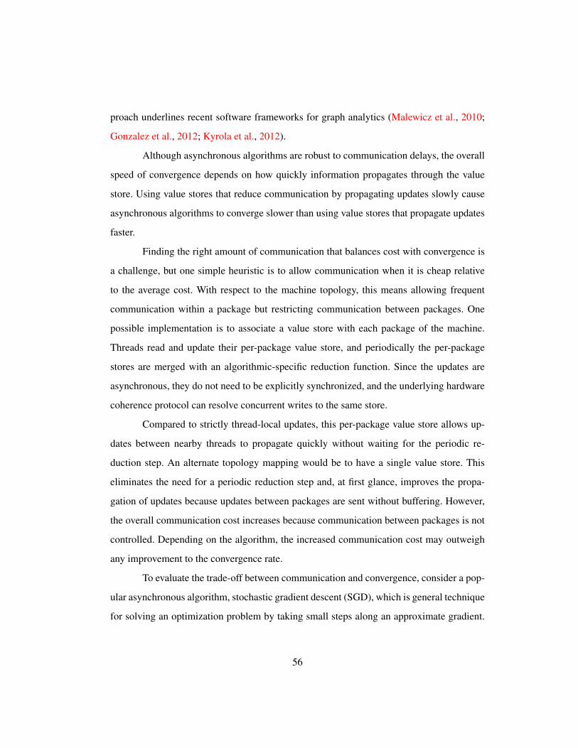
proach underlines recent software frameworks for graph analytics (Malewicz et al., 2010;

Gonzalez et al., 2012; Kyrola et al., 2012).

Although asynchronous algorithms are robust to communication delays, the overall

speed of convergence depends on how quickly information propagates through the value

store. Using value stores that reduce communication by propagating updates slowly cause

asynchronous algorithms to converge slower than using value stores that propagate updates

faster.

Finding the right amount of communication that balances cost with convergence is

a challenge, but one simple heuristic is to allow communication when it is cheap relative

to the average cost. With respect to the machine topology, this means allowing frequent

communication within a package but restricting communication between packages. One

possible implementation is to associate a value store with each package of the machine.

Threads read and update their per-package value store, and periodically the per-package

stores are merged with an algorithmic-specific reduction function. Since the updates are

asynchronous, they do not need to be explicitly synchronized, and the underlying hardware

coherence protocol can resolve concurrent writes to the same store.

Compared to strictly thread-local updates, this per-package value store allows up-

dates between nearby threads to propagate quickly without waiting for the periodic re-

duction step. An alternate topology mapping would be to have a single value store. This

eliminates the need for a periodic reduction step and, at first glance, improves the propa-

gation of updates because updates between packages are sent without buffering. However,

the overall communication cost increases because communication between packages is not

controlled. Depending on the algorithm, the increased communication cost may outweigh

any improvement to the convergence rate.

To evaluate the trade-off between communication and convergence, consider a pop-

ular asynchronous algorithm, stochastic gradient descent (SGD), which is general technique

for solving an optimization problem by taking small steps along an approximate gradient.

56

SGD itself can be used to solve many different problems. For this case study, consider the

problem of learning a linear support vector machine (SVM) model for use in binary classi-

fication (see Section 2.3). Briefly, the input to the algorithm is a set of documents xi ∈ X ,

which are vectors of length M , and a label yi ∈ −1, 1 for each document indicating

whether the document is a positive or negative example of classification being learned. The

output is a vector w also of length M such that w · xi · yi > 0 for as many documents as

possible. The vector w can be used to classify new documents by computing the product

w · xj . If this value is greater than zero, the document is a positive example; otherwise, it

is a negative example. SGD solves this problem by starting at an initial guess for w and

processing documents individually. Each document processed produces an update to w,

and eventually w converges to w. Parallelism exists in this algorithm when documents are

sparse, which means not all elements of w need to be updated for each document.

Since SGD is an asynchronous algorithm, it can be implemented with many dif-

ferent value stores. Consider four possible implementations, three of which have been pre-

viously considered for parallelizing SGD. The first is thread-local value stores with peri-

odic merging (Agarwal et al., 2014). The second is “hogwild” updates (Recht et al., 2011)

where there is a single value store updated by all threads, and the hardware coherence sorts

out concurrent updates. The third is stale synchronous (Ho et al., 2013) in which execu-

tion proceeds in rounds. Locations read in one round return values written in the previous

round. Writes to locations are accumulated. When a round ends, the accumulated writes

are merged to form the values to be read in the following round. The new implementation

is a store using the diffracted state methodology introduced in the previous section. It uses

per-package value store replicas with high value updates communicated between packages

in a ring topology. In contrast to previous value store implementations, the diffracted state

store explicitly maps data to the memory hierarchy.

Figure 5.5 shows how accuracy (i.e., prediction quality) improves with time for a

small input (news20 (Keerthi and DeCoste, 2005): 20 K documents, 1.4 M features) and a

57

m2x4 m4x10 numa8x4

0.80

0.85

0.90

0.95

1.00

0.80

0.85

0.90

0.95

1.00

0.80

0.85

0.90

0.95

1.00

0.0 0.5 1.0 0.0 0.5 1.0 0.0 0.5 1.0

Time (s)A

ccura

cy

Wild

Local

DS

Stale DS

Wild

Local

Stale

Wild

DS Stale

Local

Figure 5.5: Convergence of SVM-SGD training on small input on three different machineswith maximum number of threads on each machine

large data set (webspam (Webb et al., 2006): 350 K documents, 16.6 M features). The ma-

chines used for the evaluation are the same as in Section 5.3. Prediction accuracy is mea-

sured by training on four-fifths of the documents and testing on the last fifth. For reference,

the widely used liblinear library (Fan et al., 2008) takes about 0.833 seconds to achieve

an accuracy of 0.965 on the small input on machine m4x10 and 93.9 seconds to achieve

an accuracy of 0.993 on the large input. However, it uses a different training algorithm,

GLMNET, which will be discussed shortly.

Value store implementations that communicate frequently like the diffracted state

(DS) and hogwild (Wild) approaches improve their accuracy more quickly than approaches

that communicate less frequently like bounded staleness (Stale) and thread-local stores

(Local). Convergence results for the large input are omitted because all of the implemen-

tations except for stale synchronous converged to the same accuracy (≈ 0.985) after one

round of SGD updates. The stale synchronous approach failed to converge. Thus, for the

large input, performance is determined by how fast each implementation can do one round

of SGD updates.

Figure 5.6 shows speed-up for executing one round of SGD, where the baseline is

the time of the best implementation for one thread. For reference, the time to execute one

SGD round with the diffracted state value store on machine m4x10 with 40 threads is 0.048

seconds for the small input and 1.3 seconds for the large input. Comparing Figure 5.5 and

58

Stale

LocalDS

Wild

Stale

Local

Wild

DS

Stale

Local

WildDS

Wild

Local

Stale

DS

Wild

StaleLocal

DS

Wild

StaleLocal

DS

m2x4, small m2x4, large

m4x10, small m4x10, large

numa8x4, small numa8x4, large

2

4

6

2.5

5.0

7.5

5

10

0

10

20

30

2.5

5.0

7.5

10.0

0

5

10

15

20

4 8 12 16 4 8 12 16

0 10 20 30 40 0 10 20 30 40

0 10 20 30 0 10 20 30

Threads

Speedup

Figure 5.6: Speedup of SVM-SGD training for one SGD round

Figure 5.6 for the small input, one sees that although the hogwild approach produces higher

quality results, it is doing so at increasing cost, as shown by the lower speedup numbers

for an SGD round. The thread-local and bounded staleness stores also have low speedups

because the overhead of merging values between rounds. On the large input, the increased

communication of the hogwild approach is not worth the cost, and it is the diffracted state

implementation that achieves the best performance.

To show the generality of the diffracted state store, consider logistic regression, an

alternate machine learning method for classification. Although SGD can be used in this case

as well, it requires frequent evaluation of transcendental functions, which can be avoided by

using a different method called GLMNET (Friedman et al., 2010). The core of the method is

computing an approximate Hessian, which has a similar data access pattern as SGD except

that iterations are over keywords nodes and updates are to values on adjacent documents (in

SVM-SGD iterations are over documents and updates are to values on adjacent keywords).

59

1234 5

1

2

3 4

5

1 2 3 4 5

m4x10

0.4

0.6

0.8

1.0

30 60 90 120

Time (s)

Acc

ura

cy

DSWild

Local

Figure 5.7: Convergence of GLMNET training on large input on machine m4x10 with 40threads. Boxes indicate the min and max values observed over three runs. Boxes are labeledwith the number of Newton iterations executed so far.

Another important difference is that in SGD-SVM, the value store maintains the model pa-

rameters themselves, while in GLMNET, the value store maintains elements of the Hessian,

which will then be used by subsequent processing stages to update the model parameters.

This added level of feedback has the potential to amplify the effect of small approximation

errors.

Figure 5.7 shows the convergence of GLMNET with different approximate value

stores. The bounded staleness store timed out and is not shown. Compared to SVM-SGD,

there is more performance and quality variation as indicated by the width and height of

the boxes. On this input and number of threads, the hogwild approach does worse than

diffracted state due to the uncontrolled error introduced by racy reads and writes. This error

causes subsequent phases of GLMNET to take longer to converge, which is why the fifth

iteration with hogwild has such a wide variation in time. An unlucky interleaving of reads

and writes can have a large performance impact on downstream phases.

These results show that having a good approximate value store implementation re-

quires balancing communication costs based on the application and machine.

60

node data[N]

node idx[N]

edge dst[E]

edge data[E]

...

...

...

...

nd0 nd1

dst0 dst1 dst2

ed0 ed1 ed2

(a) Compressed sparse row(CSR) representation

node data[N]

node idx[N]

edge dst/data[E]

...

...

...dst0 dst1ed0 ed1

nd0 nd1

(b) CSR after one level of inlining

data[N+E] ...dst0 dst1ed0 ed1nd0

(c) CSR after two levels of inlining

Figure 5.8: Illustration of inlining graph data

5.5 Sparse Graphs

A common data structure is a sparse graph. The Galois system provides a variety of sparse

graph implementations based on whether the operator is a local computation or a morph. In

this way, sparse graphs can be specialized according to their expected use.

For morph operators, Galois provides a general morph graph that supports concur-

rent node and edge addition and removal. The graph is implemented as a collection of node

objects. Each node contains an array of edges that can grow dynamically. Each edge main-

tains the label data on the edge and a pointer to the neighboring node. The array of edges

stores both edges from neighbors (in-edges) and edges to neighbors (out-edges). For undi-

rected graphs, an in-edge stores a pointer to the corresponding out-edge so that updates to

an edge label on one edge are reflected in the matching edge. The memory for this graph is

allocated from the memory allocators described in Section 5.1.

The exclusive lock locations described in Section 5.2 are implemented as an addi-

tional field on each node of the graph.

When the operator is a local computation, the general morph graph implementation

61

wastes space on metadata like the resizable number of edges, which is not necessary for

local computations. In this case, the sparse graph behaves like a sparse matrix and similar

implementations can be used. Figure 5.8 shows one popular sparse matrix representation,

compressed sparse row (CSR). It uses four fixed-size arrays: one array for the node data

(labels), one index array indicating where the edges for a node can be found, one array

for the ids of the neighboring nodes, and one array for the edge data (labels). In local

computations, the size and structure of the graph is known in advance, so the memory for

these arrays can be allocated all at once from the operating system. One small optimization

for graphs that have random access behavior is to interleave the allocation across NUMA

nodes to improve memory bandwidth.

Another optimization is to inline the arrays to increase spatial locality. The common

pattern of accessing a node and its neighbors in CSR representation requires accessing

entries in four different arrays. Inlining as is shown in Figure 5.8 can reduce the number of

memory accesses by reducing the number of arrays accessed. Users of the Galois system

can select different local computation graphs based on their desired level of inlining.

62

Chapter 6

Scheduling

Parallel programming models like Cilk (Blumofe et al., 1995) or OpenMP only provide a

small number of scheduling policies, but Section 2.3 illustrates the need for a variety of

scheduling policies for algorithms. Efficient algorithms often require application-specific

scheduling strategies. This chapter describes how the Galois system supports a variety of

scheduling policies through compositional scheduler synthesis.

6.1 Scheduler Building Blocks

This section describes two example building blocks for a scheduler: (1) a topology-aware

bag of tasks (Section 6.1.1), called distributed chunked LIFO, and (2) a topology-aware pri-

ority scheduler (Section 6.1.2), called obim. While these blocks can be used as task sched-

ulers by themselves, the intention is to use them as well as other schedulers in the com-

positional scheduler synthesis described in Section 6.2 to implement programmer-supplied

scheduling policies.

63

ChunkCore

0

Package 0

Core1

Package 1

Stack ofChunks

Core0

Core1

(a) Distributed chunkedLIFO, a topology-awarebag of tasks

LocalMap 1 3 3 7

Bag1 Bag3 Bag7

1 3 7GlobalMap

Core0

Core1

(b) Obim, atopology-awarepriority scheduler

Figure 6.1: Organization of distributed chunked LIFO and obim schedulers

6.1.1 Topology-Aware Bag of Tasks

A common scheduling abstraction is a data structure that allows concurrent insertion and re-

trieval of unordered tasks. This data structure is called a bag, and it is a basic building block

for dynamic scheduling of tasks. There are many possible implementations. One of the most

well-known is per-thread deques with randomized workstealing, which was popularized by

the Cilk system (Blumofe et al., 1995). This section describes another bag implementation,

a distributed chunked LIFO, which unlike the original Cilk scheduler, attempts to optimize

communication to follow the communication topology of a multicore processor. This is

another application of the diffracted state methodology (see Section 5.3). It is possible to

manipulate the bag in FIFO-style as well, but to keep this description simple, that possibility

is omitted here.

Figure 6.1a outlines the structure of the distributed chunked LIFO and Figure 6.2

gives pseudocode to implement its two main operations: push, which adds a task to the bag,

and pop, which retrieves a task from the bag if available.

This chapter assumes throughout that threads are bound uniquely to cores.

• Each thread has a data structure called a chunk, which is a ring-buffer that can contain

8–64 tasks (size chosen at compile time). The ring-buffer is manipulated as a stack

Portions of this chapter have previously appeared in (Nguyen and Pingali, 2011), where the Galois synthe-sis procedure was originally described.

64

1 c l a s s Dis t r i bu t edChunkedLIFO :2 / / One chunk per t h r e a d3 PerThread<Chunk∗> p e r T h r e a d45 / / Chunk embeds a n e x t p o i n t e r f o r t h e l i n k e d l i s t6 PerPackage<T h r e a d S a f e L i n k e d L i s t<Chunk∗>> p e r P a c k a g e78 / / Add a t a s k9 void push ( Task t ) :

10 / / Get t h read−l o c a l chunk11 Chunk∗& c u r = p e r T h r e a d . l o c a l ( )12 / / Push t a s k t o l o c a l chunk i f e x i s t s13 i f c u r && cur−>push ( t ) :14 re turn15 / / O therwise , chunk i s f u l l or does n o t e x i s t16 i f c u r :17 p e r P a c k a g e . l o c a l ( ) . push ( c u r )18 / / Cr ea t e a new chunk and use i t19 c u r = new Chunk20 cur−>push ( v a l )2122 / / Get n e x t t a s k23 Task pop ( ) :24 Chunk∗& c u r = p e r T h r e a d . l o c a l ( ) ;25 / / Try t h e l o c a l chunk f i r s t26 i f c u r && ! cur−>empty ( ) :27 re turn cur−>pop ( )28 / / D e l e t e empty chunk29 i f c u r :30 d e l e t e c u r31 / / Next , t r y t h e per−package l i s t32 c u r = p e r P a c k a g e . l o c a l ( ) . pop ( )33 i f c u r :34 re turn cur−>pop ( )35 / / I f no t a s k i s found , probe o t h e r packages36 f o r l s t in p e r P a c k a g e :37 / / Lock−f r e e t e s t f o r t a s k s38 i f ! l s t . empty ( ) :39 c u r = l s t . pop ( ) / / s y n c h r o n i z e d pop40 i f c u r :41 re turn cur−>pop ( )42 re turn FAIL

Figure 6.2: Pseudocode for distributed chunked LIFO

65

(LIFO). New tasks are pushed onto the ring buffer, and tasks are popped from it when

the thread needs work.

• Each package has a list of chunks. This list is manipulated in LIFO order.

• When the chunk associated with a thread becomes full, it is moved to the package-

level list.

• When the chunk associated with a thread becomes empty, the thread probes its pack-

age-level list to obtain a chunk. If the package-level list is also empty, the thread

probes the lists of other packages to find work. To reduce traffic on the inter-package

connection network, only one hungry thread hunts for work in other packages on

behalf of all hungry threads in a package.

This implementation is topology-aware because the most frequent operations use

the least cost communication paths, while less frequent operations may use more costly

communication. Threads can usually satisfy pushing or popping tasks by manipulating

thread-private chunks. Only when a per-thread chunk becomes full or empty is the per-

package linked-list manipulated. Communication between threads sharing the same pack-

age costs more than thread-private communication but costs less than communication be-

tween packages. Only in the rare case when (1) a thread is trying to pop a task, (2) its

thread-private chunk is empty, and (3) its per-package linked-list is empty does a thread use

expensive inter-package communication to find tasks in other packages.

Similar topology-aware optimizations have been proposed for per-thread deques (Guo

et al., 2010; Wang et al., 2012b; Drebes et al., 2014), and the compositional scheduler syn-

thesis described in Section 6.2 can use these schedulers, with slight modification (see Sec-

tion 6.2.3), in addition to the topology-aware bag described here. However, most prior work

in scheduling considers the problem of implementing a single, monolithic scheduler that

is used for all parallel tasks and does not consider schedulers as blocks out of which more

sophisticated schedulers are built. In the compositional scheme introduced later in this chap-

66

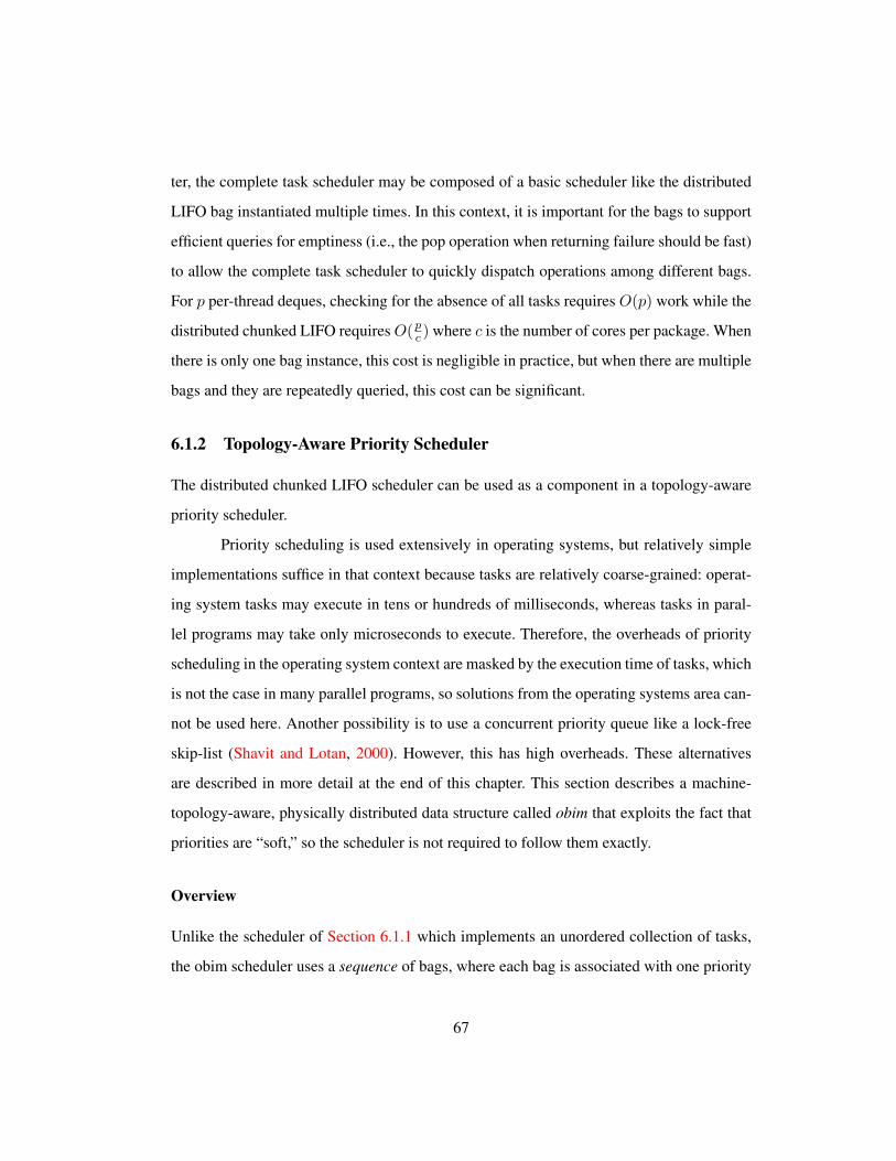
ter, the complete task scheduler may be composed of a basic scheduler like the distributed

LIFO bag instantiated multiple times. In this context, it is important for the bags to support

efficient queries for emptiness (i.e., the pop operation when returning failure should be fast)

to allow the complete task scheduler to quickly dispatch operations among different bags.

For p per-thread deques, checking for the absence of all tasks requires O(p) work while the

distributed chunked LIFO requiresO(pc ) where c is the number of cores per package. When

there is only one bag instance, this cost is negligible in practice, but when there are multiple

bags and they are repeatedly queried, this cost can be significant.

6.1.2 Topology-Aware Priority Scheduler

The distributed chunked LIFO scheduler can be used as a component in a topology-aware

priority scheduler.

Priority scheduling is used extensively in operating systems, but relatively simple

implementations suffice in that context because tasks are relatively coarse-grained: operat-

ing system tasks may execute in tens or hundreds of milliseconds, whereas tasks in paral-

lel programs may take only microseconds to execute. Therefore, the overheads of priority

scheduling in the operating system context are masked by the execution time of tasks, which

is not the case in many parallel programs, so solutions from the operating systems area can-

not be used here. Another possibility is to use a concurrent priority queue like a lock-free

skip-list (Shavit and Lotan, 2000). However, this has high overheads. These alternatives

are described in more detail at the end of this chapter. This section describes a machine-

topology-aware, physically distributed data structure called obim that exploits the fact that

priorities are “soft,” so the scheduler is not required to follow them exactly.

Overview

Unlike the scheduler of Section 6.1.1 which implements an unordered collection of tasks,

the obim scheduler uses a sequence of bags, where each bag is associated with one priority

67

level. To be concrete, this section assumes that each bag is implemented as the distributed

chunked LIFO described above, but in practice, the scheduler synthesizer can use any bag

implementation. Tasks in the same bag have identical priorities and can therefore be ex-

ecuted in any order; however, tasks in bags that are earlier in the sequence are scheduled

preferentially over those in later bags. This is shown pictorially as the Global Map in Fig-

ure 6.1b. This map is sparse since it contains bags only at entries 1, 3 and 7. Threads work

on tasks in bag 1 first; only if a thread does not find a task in bag 1 does it look for work in

the next bag (bag 3). If a thread creates a task with some priority and the corresponding bag

is not there in the global map, the thread allocates a new bag, updates the global map, and

inserts the task into that bag.

The global map is a central data structure that is read and written by all threads. To

prevent it from becoming a bottleneck and to reduce coherence traffic, each thread maintains

a software-controlled lazy cache of the global map, as shown in Figure 6.1b. Each local map

contains some portion of the global map that is known to that thread, but it is possible for a

thread to update the global map without informing other threads.

The main challenge in the design of obim is getting threads to work on early priority

work despite the distributed, lazy-cache design. This is accomplished as follows.

Implementation of global/local maps

The thread-local map is implemented by a sorted, dynamically resizable array of pairs.

Looking up a priority in the thread-local map is done using a binary search. Threads also

maintain a version number representing the last version of the global map they synchronized

with. The global map is represented as a log-based structure which stores bag-priority pairs

representing insert operations on the logical global map. Each logical insert operation up-

dates the global version number.

Updating the global map When a thread cannot find a bag for a particular priority using

only its local map, it must synchronize with the global map and possibly create a new

68

1 c l a s s Obim :2 s t r u c t Data : / / Per−t h r e a d da ta3 Bag∗ c u r r e n t / / C u r r e n t bag4 i n t c u r P r i o r i t y / / C u r r e n t p r i o r i t y5 i n t l a s t V e r s i o n / / L a s t v e r s i o n s yn ce d6 OrderedMap<i n t , Bag∗> loca lMap / / Copy o f g l o b a l s t a t e78 PerThread<Data> p e r T h r e a d9 T h r e a d S a f e V e c t o r<P a i r<i n t , Bag∗>> masterLog

10 i n t m a s t e r V e r s i o n11 S p i n l o c k mas te rLock1213 / / Add a t a s k w i t h a p r i o r i t y14 void push ( Task t , i n t p r i o r i t y ) :15 Bag∗ b16 Data& d = p e r T h r e a d . l o c a l ( )17 / / Check cache18 i f d . c u r P r i o r i t y == p r i o r i t y && d . c u r r e n t :19 b = t l d . c u r r e n t20 e l s e :21 b = u p d a t e L o c a l O r C r e a t e ( d , p r i o r i t y )22 b−>push ( t )23 / / Update p r i o r i t y i f n e c e s s a r y24 i f p r i o r i t y < t l d . c u r P r i o r i t y :25 d . c u r r e n t = b26 d . c u r P r i o r i t y = p r i o r i t y2728 Task pop ( ) :29 Data& d = p e r T h r e a d . l o c a l ( )30 i f d . c u r r e n t && (++ d . popCount % s c a n P e r i o d ) != 0 :31 Task t = t l d . c u r r e n t−>pop ( )32 i f t != FAIL :33 re turn t34 r e p l a y L o g ( d ) / / Fa i l ed , up da t e l o g35 re turn s can ( d )

Figure 6.3: Pseudocode for obim; auxiliary functions in Figure 6.4

69

1 c l a s s Obim :2 / / . . .34 / / Search f o r e a r l i e r p r i o r i t y work5 Task scan ( Data& d ) :6 i n t s c a n S t a r t7 i f u s i n g B a c k S c a n P r e v e n t i o n :8 s c a n S t a r t = min ( [ x . c u r P r i o r i t y f o r x in p e r T h r e a d . p a c k a g e L o c a l ( ) ] )9 e l s e :

10 s c a n S t a r t = 011 f o r p in r a n g e ( s c a n S t a r t , d . loca lMap . maxKey + 1 ) :12 Bag∗ b = loca lMap . f i n d ( p )13 i f b :14 Task t = b−>pop ( )15 i f t != FAIL :16 d . c u r P r i o r i t y = p17 d . c u r r e n t = b18 re turn t19 re turn FAIL2021 / / Find e n t r y i n l o c a l cache or c r e a t e e n t r y i n g l o b a l map22 Bag∗ u p d a t e L o c a l O r C r e a t e ( Data& d , i n t p r i o r i t y ) :23 whi le t rue :24 r e p l a y L o g ( d )25 i f d . loca lMap . f i n d ( p r i o r i t y ) :26 re turn d . loca lMap . f i n d ( p r i o r i t y )27 i f maste rLock . t r y L o c k ( ) :28 break29 / / S e r i a l i z a t i o n p o i n t30 r e p l a y L o g ( d )31 i f d . loca lMap . f i n d ( p r i o r i t y ) :32 re turn d . loca lMap . f i n d ( p r i o r i t y )33 / / Update l o g34 i n t v = m a s t e r V e r s i o n + 135 Bag∗ b = new Bag36 mas te rLog [ v ] = P a i r ( p r i o r i t y , b )37 memoryBar r i e r ( )38 m a s t e r V e r s i o n = v39 d . loca lMap . i n s e r t ( p r i o r i t y , b )40 mas te rLock . un loc k ( )41 re turn b4243 / / Update l o c a l cache from l o g44 void r e p l a y L o g ( Data& d ) :45 i n t m = m a s t e r V e r s i o n46 f o r i in r a n g e ( d . l a s t V e r s i o n , m) :47 d . loca lMap . i n s e r t ( mas te rLog [ i ] )48 d . l a s t V e r s i o n = m

Figure 6.4: Auxiliary functions for Figure 6.3

70

mapping there. This is accomplished in the updateLocalOrCreate method (see Figure 6.4

line 22). A thread replays the global log from the point of the thread’s last synchronized

version to the end of the current global log. This inserts all newly created mappings into

the thread’s local map. If the right mapping is still not found, the thread will acquire a write

lock, replay the log again, and append a new mapping to the global log and its local map.

The write lock ensures that only one mapping exists for any priority value. Some care must

be taken with the implementation of the global log to ensure that the log can be appended

in the presence of concurrent readers without requiring locks.

Pushing a task A thread pushing a task uses its local map to find the correct bag into

which to insert. Failing that, the thread updates its local map from the global map, as above,

possibly creating a new mapping, and it uses the found or created bag for the push operation.

Retrieving a task To keep close to the ideal schedule, all threads must be working on

important (earliest priority) work. When a task is executed, it may create one or more new

tasks with earlier priority than itself because priorities are arbitrary application-specific

functions. If so, the thread executes the task with the earliest priority and adds all the other

tasks to the local map. Threads search for tasks with a different priority only when the bag

in which they are working becomes empty or if a heuristically defined number of pops has

occurred; the threads then scan the global map looking for important work. This procedure

is called the back scan.

Because a scan over the entire global map can be expensive, especially if there

are many bags, an approximate consensus heuristic, called back scan prevention, is used

to locally estimate the earliest priority work available and to prevent redundant scans for

earlier priority work. Each thread publishes the priority it is working at by writing it to

shared memory. When a thread needs to scan for work, it looks at this value for all threads

that share the same package and uses the earliest priority it finds to start the scan for work.

To propagate information between packages, in addition to scanning all the threads in its

71

package, one leader thread per package will scan the other package leaders. This restriction

allows most threads to incur only a small amount of local communication. Once a thread

has a starting point for a scan, it simply tries to pop work from each bag from the scan point

onwards.

Back scan prevention is effective because, in many uses of priority scheduling, tasks

generate work at the same or later priority, and back scan prevention can limit the scan for

earlier priority tasks to just a few bags.

This scheduler is topology-aware because push and pop operations are most likely

satisfied by accessing thread-private chunks in a distributed chunked LIFO via operations

on the bag at the current priority. The next most frequent operation is using the ordered map

to find the bag into which to insert new work. The local map cache allows this operation

to also be core-private with high probability. Finally, threads must from time to time find

an earlier priority bag to retrieve work from. This requires some communication between

threads to find the global minimum. Although this could done on mostly read-only data,

adding some communication in the form of a topology-aware, approximate, autonomous

consensus algorithm greatly reduces the total time spent looking for the least bag in the

system and reduces cases where a thread works on one priority even though earlier priority

work has been enqueued (i.e., priority inversions).

Alternatively, one may use a more inductive argument to show that this scheduler

is topology-aware. The push and pop operations mainly consist of finding an early priority

bag and applying the appropriate operation to the bag. The bag is already known to be

topology-aware, so one must only show that finding early priority bags is topology-aware.

Evaluation of Design Choices

This section evaluates the design choices of the obim scheduler by comparing the perfor-

mance of several de-optimized variants. Figure 6.5b lists the variants, which focus on two

main optimizations: (1) the use of per-package linked-list of chunks and (2) back scan

72

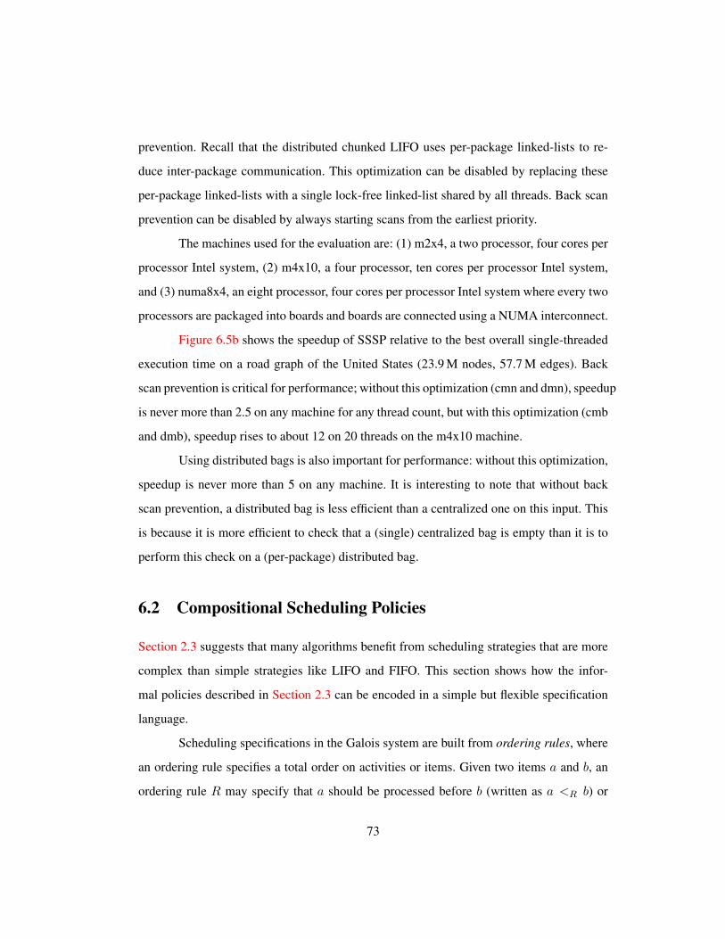
prevention. Recall that the distributed chunked LIFO uses per-package linked-lists to re-

duce inter-package communication. This optimization can be disabled by replacing these

per-package linked-lists with a single lock-free linked-list shared by all threads. Back scan

prevention can be disabled by always starting scans from the earliest priority.

The machines used for the evaluation are: (1) m2x4, a two processor, four cores per

processor Intel system, (2) m4x10, a four processor, ten cores per processor Intel system,

and (3) numa8x4, an eight processor, four cores per processor Intel system where every two

processors are packaged into boards and boards are connected using a NUMA interconnect.

Figure 6.5b shows the speedup of SSSP relative to the best overall single-threaded

execution time on a road graph of the United States (23.9 M nodes, 57.7 M edges). Back

scan prevention is critical for performance; without this optimization (cmn and dmn), speedup

is never more than 2.5 on any machine for any thread count, but with this optimization (cmb

and dmb), speedup rises to about 12 on 20 threads on the m4x10 machine.

Using distributed bags is also important for performance: without this optimization,

speedup is never more than 5 on any machine. It is interesting to note that without back

scan prevention, a distributed bag is less efficient than a centralized one on this input. This

is because it is more efficient to check that a (single) centralized bag is empty than it is to

perform this check on a (per-package) distributed bag.

6.2 Compositional Scheduling Policies

Section 2.3 suggests that many algorithms benefit from scheduling strategies that are more

complex than simple strategies like LIFO and FIFO. This section shows how the infor-

mal policies described in Section 2.3 can be encoded in a simple but flexible specification

language.

Scheduling specifications in the Galois system are built from ordering rules, where

an ordering rule specifies a total order on activities or items. Given two items a and b, an

ordering rule R may specify that a should be processed before b (written as a <R b) or

73

m2x4 m4x10 numa8x4

dmncmn

cmb

dmb

dmncmncmb

dmb

dmncmncmb

dmb

0

3

6

9

12

2 4 6 8 0 10 20 30 40 0 10 20 30

Threads

Sp

ee

du

p

(a) Speedup of variants on road graphBack Scan Prevention

No Yes

Centralized Bag cmn cmbDistributed Bag dmn dmb (obim)

(b) Obim variants

Figure 6.5: Scaling of obim and its variants for SSSP application

vice versa (b >R a), or it may leave the order unspecified (a =R b). For example, if items

have integer priorities, an ordering rule A1 may order them in ascending priority order;

the relative order of items with the same priority is left unspecified by A1. Ordering rules

can be composed sequentially in a manner similar to lexicographic ordering: a sequence

D = R1R2R3 . . . is itself an ordering rule that first orders items according to R1; if two

items are not strictly ordered by R1, they are ordered according to R2, etc. For example, if

F1 orders items in FIFO order, thenA1 F1 denotes the order in which items are processed in

increasing priority order and items with the same priority are processed in FIFO order. For

the synthesis procedure described in Section 6.2.1, it is convenient to distinguish between

final rules, which are rules that appear last in an ordering sequence, and non-final rules.

As discussed in Section 2.3, some implementations of irregular algorithms maintain

separate global and thread-local worksets, so it is natural to use different ordering rules for

them. A scheduling specification can have both a global ordering rule and a local ordering

rule. The global rule is applied to the initial set of items, and the local rule is applied to each

74

thread-local workset, which holds items created dynamically by the corresponding thread.

A thread accesses the global workset only when its local workset is empty. Continuing the

previous example, if L1 is last-in-first-out (LIFO) order, then global order A1F1 and local

order L1 specify that global items are processed as before, and local items are processed in

LIFO order.

Figure 6.6 gives the syntax rules for scheduler specifications. T is the type of items.

Figure 6.7 gives the semantics. The meaning of an ordering rule R is given as a function

over items a and b that is true iff a <R b. The relation < is the standard order on integers

and reals.1 For the FIFO and LIFO rules, we define an auxiliary function time that maps

an item to an integer according to when the item is added to the scheduler. For the first item

x1 added to the scheduler, time(x1) = 0; for the second item x2, time(x2) = 1, and so

on. fU is an injective function mapping items to integers; this function essentially encodes

a random permutation of items. The function fD should be consistent with a total order.

Figure 6.8 shows the specifications of the scheduling policies discussed in Sec-

tion 2.3. When a specification has an empty local ordering, the figure omits the global and

local tags. The BRIO specification assumes that items have already been assigned rounds

according to the random distribution described in Section 2.3. In the original delta-stepping

algorithm (Meyer and Sanders, 1998), edges relaxations are divided into light (i.e., < ∆)

and heavy requests, and for a particular bucket, light requests are processed first, including

any light requests enabled by processing a request, before moving on to the heavy requests.

To process light requests before heavy ones, the delta-stepping specification splits each

bucket into two: one part for the light requests and one part for the heavy requests.1 Instead of binary relation on pairs of items T × T → bool, the semantics of a rule could be a function

that maps a set of items to a sequence of sets of items SetT → SeqSetT. This allows a cleaner formaldevelopment (e.g., the non-syntactic a and b terms can be removed). We adopt the current approach because itseems more intuitive for programmers.

75

P ::= Global:D Local:D SpecificationD ::= RNF

∗ RF? Ordering ruleRF ::= FIFO Final rule

| LIFO| Random

RNF ::= ChunkedFIFO(k) Non-final rule| ChunkedLIFO(k)

| Ordered(fD)

| OrderedByMetric(fM)

k IntegerfD T× T→ bool

fM T→ R

Figure 6.6: Scheduling specification syntax

6.2.1 Synthesis

It is straightforward to implement sequential schedulers for policies specified in the lan-

guage described in Section 6.2. Each rule can be implemented by a workset, which is an

object with the following methods:

• void push(Task t ) — adds an item to the workset

• Task pop() — removes and returns the next item to execute; if there are no items left,

returns a FAIL value distinct from all items added to the workset

Items are added to the workset by invoking the push method, which returns the value void

when it completes. To get items from the workset, the pop method is invoked; if this method

invocation does not find any items in the workset, it returns a unique FAIL value.

The goal of this section is to synthesize concurrent worksets that implement this

functionality. One approach is to compose a set of library components, each of which is a

workset by itself. There is a workset for each final rule; non-final rules are implemented by

worksets parameterized by a function that constructs instances of the next workset in the

ordering sequence, the inner workset.

76

JFIFOK(a, b) = time(a) < time(b)

JLIFOK(a, b) = time(a) > time(b)

JRandomK(a, b) = fU(a) < fU(b)

JChunkedFIFO(k)K(a, b) = btime(a)/kc < btime(b)/kcJChunkedLIFO(k)K(a, b) = btime(a)/kc > btime(b)/kc

JOrdered(fD)K(a, b) = fD(a, b)

JOrderedByMetric(fM)K(a, b) = fM(a) < fM(b)

JR1R2 . . .K(a, b) =

JR2 . . .K(a, b) if a =R1 b

JR1K(a, b) otherwise

Figure 6.7: Scheduling rule semantics

However, a naive implementation along these lines can be incorrect in a concurrent

setting, as will be seen in Section 6.2.2, and the result may not satisfy any intuitive notion

of correctness such as linearizability (Herlihy and Wing, 1990). To address this problem,

Section 6.2.3 proposes a relaxed correctness condition that requires modifications to the

semantics of worksets and to how they are used by clients.

Section 6.2.4 discusses two important consequences of this relaxed condition: (1)

all final scheduling policy rules in Section 6.2 have implementations that satisfy the relaxed

condition, and (2) non-final worksets satisfy the relaxed condition assuming only that their

inner worksets satisfy the relaxed condition. This permits compositional construction of

worksets.

Section 6.2.5 discusses a preliminary implementation of scheduling policies in Java

in an early version of the Galois system and several optimizations to improve the perfor-

mance of the synthesized worksets.

6.2.2 Problems with Naive Composition

To understand the issues that arise in composing worksets, consider the implementation of

the bucket-based scheduler in lines 1–18 of Figure 6.9. This is one possible implementation

of the OrderedByMetric rule (the obim scheduler of Section 6.1.2 is another). Lines 20–25

77

Specification Used by

DMR OrderedByMetric(λt.minangle(t)) FIFO Triangle angle (AS2)(Shewchuk, 1996)

Global: ChunkedFIFO(k) Local: LIFO Local stack (AS1)(Kulkarni et al., 2008)

DT OrderedByMetric(λp. round(p)) ChunkedFIFO(k) BRIO (AS1) (Amentaet al., 2003)

Random Random (Clarksonand Shor, 1989)

PFP FIFO FIFO (Goldberg andTarjan, 1988)

OrderedByMetric(λn. − height(n)) FIFO HL order (AS1)(Cherkassy andGoldberg, 1995)

PTA FIFO LRF (Pearce et al.,2003)

(empty) Split worklists (BS-F)(Nielson et al., 1999;Hardekopf and Lin,2007)

SSSP FIFO Bellman-Ford (Bell-man, 1958; Ford andFulkerson, 1962)

OrderedByMetric(λn. b2 ∗ w(n)/∆c+ (light(n) ? 0 : 1)) FIFO Delta-stepping (AS1)(Meyer and Sanders,1998)

Ordered(λa, b. w(a) ≤ w(b)) Dijkstra (AS2) (Dijk-stra, 1959)

Figure 6.8: Application-specific scheduling specifications

78

1 c l a s s B u c k e t e d S c h e d u l e r :2 Vector<Bag> b u c k e t s3 i n t c u r s o r45 void push ( Task t ) :6 i n t i n d e x = f l o a t T o I n t (fM(t) )7 b u c k e t s [ i n d e x ] . push ( t )8 i f i n d e x < c u r s o r : c u r s o r = i n d e x9

10 Task pop ( )11 Task t = FAIL12 whi le c u r s o r < b u c k e t s . s i z e ( ) :13 t = b u c k e t s [ c u r s o r ] . pop ( )14 i f t == FAIL :15 c u r s o r ++16 e l s e :17 break18 re turn t1920 B u c k e t e d S c h e d u l e r s c h e d u l e r21 ThreadPoo l . f o r k (N) / / spawn N t h r e a d s22 Task i t em23 whi le ( i t em = s c h e d u l e r . pop ( ) ) != FAIL :24 operator . c a l l ( i tem , s c h e d u l e r )25 ThreadPoo l . j o i n (N)

Figure 6.9: Naive bucketed scheduler

show how this scheduler might be used in a parallel runtime system. The runtime system

manages threads and assigns them work. The workset creates an array of inner worksets

and processes each inner workset in ascending order. This workset is essentially an imple-

mentation of a priority queue in which the range of keys is known a priori; there is one

inner workset (bucket) for each key value. Similar worksets have been used in a variety

of sequential (Amenta et al., 2003; Cherkassy and Goldberg, 1995; Shewchuk, 1996) and

parallel implementations (Meyer and Sanders, 1998) of irregular algorithms.

Unfortunately, the workset in Figure 6.9 can exhibit incorrect behavior because it is

possible for items to be inserted into the workset but never retrieved. Consider two threads

T1 and T2, where T1 is executing the pop method and T2 is executing the push method. The

following sequence of events may take place:

79

1. T1 executes line 13. The cursor value is i, and the pop method on buckets[i] returns

FAIL.

2. T2 executes lines 6–8. The value of index = i, so an item is added to buckets[i].

3. T1 executes lines 14 and 15 of the pop method, incrementing cursor.

Clearly, the item added by T2 is now lost. The race exists even if each line of the

implementation is atomic, so that reading and updating the cursor on line 15 or increment-

ing its value on line 15 is performed atomically. To use this implementation correctly in a

concurrent context, one must ensure that when poll moves to the next bucket, no thread is

adding an element to an earlier priority bucket.

A second problem is that even if the methods of a workset are linearizable, the

workset cannot be used to directly control the execution of threads in the client. In the

client code of Figure 6.9, a thread stops processing items when the workset returns FAIL,

and then waits for the rest of the threads to join it. However, one possible scenario is (1) all

threads but one are waiting at the barrier, (2) the workset is empty, and (3) while processing

the last item, the last thread adds several items to the workset. The waiting threads now

need to wake up and re-enter the parallel loop, but this will not happen in the client code

of Figure 6.9. Abstractly, the problem is one of termination detection: when should parallel

execution stop? An eager termination detection algorithm risks having threads idle when

there is work to be done. A lazy algorithm will wait needlessly when there is no work. A

naive client of a concurrent workset will generally be too eager, so parallel runtime systems

need to have separate mechanisms for termination detection.

These observations can be summarized as follows.

• In general, simple compositions of worksets do not produce correct concurrent work-

sets.

• Composition of concurrent worksets is problematic even in absence of having to

maintain a particular order of items.

80

• Worksets are used by parallel runtime systems. In some cases, runtime systems them-

selves separately implement stronger properties like termination detection that over-

lap with some workset functionality.

6.2.3 Relaxed Concurrent Semantics

This section describes a solution to the problem of composing worksets that takes advantage

of the fact that scheduling specifications for unordered algorithms are inherently “fuzzy”

and are intended as suggestions to the runtime system rather than as commands that must

be followed exactly. At a high level, the idea is the following.

• Relax the behavior of the pop method so that in a parallel setting, it may return a dif-

ferent item than the one it would have returned in a sequential setting. In addition, pop

may return FAIL even when there are still items in the workset. These modifications

permit us to implement pop with low overhead.

• To compensate for the relaxed behavior of pop, introduce a new method pop-s that

is similar to pop but is never executed concurrently with other invocations. It returns

FAIL only when the workset is truly empty.

Intuitively, if most items are retrieved from the workset using the pop method, and

pop-s is used infrequently to determine if the workset is truly empty, the resulting scheduler

is both correct and efficient. This section formalizes this behavior, and Section 6.2.4 shows

how this behavior is closed under composition.

A workset is modeled by its history H , which is a finite sequence of events, where

an event is either (1) a method invocation, (2) a response to a method invocation, or (3) a

special termination event, 〈term〉. The invocation on object o of method m with arguments

a, b, . . . by thread T is written as 〈o.m(a, b, . . . ) T 〉; the response to method m with return

value r is written as 〈o.m(a, b, . . . )/r T 〉; The unit return value is written as void. An

invocation 〈o1.m1(a1, b1, . . . ) T1〉 matches a response 〈o2.m2(a2, b2, . . . )/r T2〉 if o1 =

81

o2, m1 = m2, a1 = a2, b1 = b2 and so on, and T1 = T2. Objects and/or threads are

omitted if they are clear from context. Terms x1, x2, . . . are variables over arguments or

return values.

An invocation is pending in H if it has no matching response. A history is whole

if it has no pending invocations and it contains exactly one termination event and that is

the last event in the history. A history restricted to object o or thread T is the subsequence

with only events on o or by T respectively and possibly a termination event. Without loss

of generality, items are assumed to be unique. The notation a →H b denotes that event a

precedes event b in history H; when the history is clear from context, this is written a→ b.

Property 6.1 is a formal description of the behavior of pop and pop-s.

Property 6.1 (Weak Bag). A history H models a weak bag if the following are true:

B1. There is an injective functionM from non-FAIL response events e1 = 〈pop()/x1 T1〉

or e1 = 〈pop-s()/x1 T1〉 to invocation events e2 = 〈push(x2) T2〉 such that (1)

M(e1) = e2, (2) x1 = x2, and (3) e2 → e1.

B2. For each invocation event e = 〈pop-s() T 〉 of pop-s in H = H1, e,H2, there are no

pending invocations in H1.

B3. For each FAIL response event e = 〈pop-s()/null T 〉 of pop-s in H = H1, e,H2,

H1 satisfies condition B1 and M is a bijective function.

Condition B1 states that (1) items returned by pop and pop-s must have been added

earlier by the push method and (2) a given item can only be returned once. Both require-

ments are captured by the injective function M . Condition B2 states that pop-s cannot

be invoked when there are pending method invocations. Condition B3 states that if pop-s

returns FAIL, all previously pushed items have been retrieved by pop or pop-s, and the

workset is truly empty. This is captured by requiring M to be a bijective function.

A workset is correct if it only generates whole histories satisfying Property 6.1.

It is the responsibility of the client to use the workset properly by never invoking pop-s

82

concurrently with other methods. This form of correctness may seem particularly weak

since it does not refer to the sequential ordering semantics. However, we have found it

useful because it includes many natural compositions of worksets as well as most hand-

written schedulers. A linearizable bag is a correct workset if one considers pop-s the same

as pop. Likewise, a bag with a single lock guarding all its methods is also a correct workset.2

One correct workset and its proper use by a runtime system is the following modi-

fication of Figure 6.9. Before line 25, the runtime system should call pop-s; if the returned

value is a non-FAIL item, the system should process that item and go to line 23 to con-

tinue execution. The pop-s method should walk the bucket array calling poll-s on each inner

workset and return the first non-FAIL item if it exists.

The implementations in the Galois system of the final rules in Figure 6.6 satisfy

Property 6.1 since the LIFO and FIFO rules are implemented by a linearizable stack and

queue respectively, and the Random rule is implemented with a resizable array and all

method invocations are protected by a single lock.

6.2.4 Workset Composition

This section summarizes how the implementations of the non-final rules in Figure 6.6 sat-

isfy Property 6.1, assuming they are parameterized by correct worksets, and gives a detailed

description for one non-final rule, OrderedByMetric. The correctness of other worksets is

briefly summarized.

Theorem 6.1 models the behavior of the OrderedByMetric workset by its history

with respect to its inner worksets. Theorem 6.2 shows how objects that generate such histo-

ries are correct worksets.

Theorem 6.1 (OrderedByMetric). Let o be an instance of the OrderedByMetric workset in

Figure 6.9 modified so that each thread maintains a thread-local cursor variable and pop-s

walks all the buckets calling pop-s on each inner workset. Let W = w1, w2, . . . , wn be2It is possible to introduce deadlock when arbitrarily composing worksets with locks. However, composi-

tions based on Theorem 6.2 whose implementations are themselves wait-free do not introduce deadlocks.

83

the set of correct worksets contained in the buckets. The workset o only generates whole

histories containing the following non-overlapping sequences when restricted to thread T

for all threads:

D1. 〈o.push(x)〉,

〈w.push(x)〉, 〈w.push(x)/void〉,

〈o.push()/void〉.

D2. 〈o.pop()〉,

(〈w∗.pop()〉, 〈w∗.pop()/FAIL〉)∗,

〈w.pop()〉, 〈w.pop()/x〉,

〈o.pop()/x〉 where x 6= FAIL.

D3. The above with pop() replaced with pop-s().

D4. 〈o.pop()〉,

(〈w∗.pop()〉, 〈w∗.pop()/FAIL〉)∗,

〈o.pop()/FAIL〉.

D5. 〈o.pop-s()〉,

〈w1.pop-s()〉, 〈w1.pop-s()/FAIL〉, . . . ,

〈wn.pop-s()〉, 〈wn.pop-s()/FAIL〉,

〈o.pop-s()/FAIL〉.

Proof. Note that the only objects shared between threads executing methods of o are the

inner worksets in W , represented in Figure 6.9 as the variable buckets. Thus, it is sufficient

to only consider sequential executions of o.

The push method clearly satisfies clause D1.

The pop method may either return FAIL or a non-FAIL value. In the case of

FAIL, each inner workset visited returns FAIL, and o satisfies clause D4. In the case of a

non-FAIL value, there are some number of inner worksets that return FAIL and exactly

one that returns a non-FAIL value. This satisfies clause D2.

84

The pop-s method is the same as the pop method except that it visits all the inner

worksets in W . By reasoning similar to the pop method, the pop-s method must satisfy

clauses D3 or D5.

Theorem 6.2 (OrderedByMetric is correct). Whole histories H satisfying Theorem 6.1

model a weak bag.

Proof. Consider each condition of Property 6.1 in turn.

First, H satisfies condition B1. Without loss of generality, consider events of pop;

events of pop-s behave similarly. From clauses D2 and D4, the only time the workset o

produces a non-FAIL response e1 = 〈o.pop()/x1〉 is when one of its correct worksets

w ∈ W produces a response f1 = 〈w.pop()/x1〉. There is exactly one event e1 for each

event f1 and vice versa. Let M1 be the bijective function from events of the form e1 to

events of the form f1. From clause D1, there is exactly one event f2 = 〈w.push(x2)〉 for

each event e2 = 〈o.push(x2)〉 and vice versa. Let M2 be the bijective function from events

of the form f2 to events of the form e2.

We now show there exists an injective function MC such that MC(e1) = e2, x1 =

x2 and e1 → e2. By definition, M1(e1) = f1 = 〈w.pop()/x1〉. Since w is a correct

workset, there exists an injective function Mw such that Mw(f1) = f2 = 〈w.push(x1)〉

and f2 → f1. Let M be the expansion of Mw over the range of all w ∈ W . The ranges of

Mw1 , . . . ,Mwn are disjoint and each Mw is an injective function so M is also an injective

function (see Figure 6.10). By definition, M2(f2) = e2 = 〈o.push(x1)〉. Let MC be the

composed function M2 M M1. MC is injective because M is injective and M1 and M2

are bijective. MC(e1) = e2 by function composition. From clauses D1 and D2, e2 → f2

and f1 → e1, and by the correctness of w, f2 → f1; so, by transitivity, e2 → e1.

Second,H satisfies condition B2. Clients of o do not invoke o.pop-s() concurrently.

From clauses D3 and D5, it is clear that if there are no pending invocations immediately

before o.pop-s() is invoked, then there will be no pending invocations immediately before

w.pop-s() for all w ∈W .

85

M

w

M M

M

1 2

1

wMn

...

o.popw.pop w.push

o.push

Figure 6.10: Relationship between M1, M and M2 in the proof of Theorem 6.2

Finally, H satisfies condition B3. From above, MC satisfies condition B1 and is an

injective function from non-FAIL pop and pop-s responses to push invocations on o. We

now show that when o produces the FAIL response 〈o.pop-s()/FAIL〉, MC is a bijection

as well. From clause D5, if o produces a FAIL response, allw ∈W have produced a FAIL

response as well. Thus, M is a bijection, and correspondingly, MC is one as well.

The ChunkedFIFO rule is implemented with a single linearizable (global) queue

whose elements (chunks) are instances of the inner workset. Each inner workset contains at

most k items. Each thread maintains a thread-local chunk to pop from. When the chunk is

empty, the thread pops from the global queue for the next chunk. Each thread also maintains

a thread-local chunk to push to. When the chunk is full, the thread pushes it to the global

queue and creates a new empty chunk to push to. The pop-s method walks each thread-local

chunk and the global queue calling pop-s on each.

Theorem 6.2 does not immediately apply because chunks are created and discarded

dynamically. One modification would be to keep track of all the chunks ever created. How-

ever, one observation is that chunks are accessed by at most one thread at a time, and they

are discarded when they are empty, which can be determined by invoking pop-s on the

chunk. Empty chunks will never contain any more items. Thus, discarded chunks do not

affect the eventual correctness of the workset. Only chunks that may contain items matter,

which are precisely those traversed by pop-s.

86

The ChunkedLIFO rule is implemented similarly to ChunkedFIFO except with a

linearizable stack.

The Ordered rule is implemented with a concurrent heap with additional locks to

protect the inner worksets. Showing the correctness of its implementation is beyond the

scope of this chapter because it uses commutativity conditions to reduce the granularity of

the locking (Kulkarni et al., 2011).

Although not a rule per se, the composition of a global and local rule, used to imple-

ment global and local orders in specifications, is implemented with worksets as well. There

is one workset that implements the global rule and thread-local worksets that implement the

local rule. Initial work is pushed to the global workset, while newly created work is pushed

to the thread-local workset. New work is retrieved from the thread-local workset, if possi-

ble, and from the global workset otherwise. For proving correctness, this implementation

can be viewed as a refinement of a chunked workset where chunks are never discarded but

are instead refilled from the global workset.

6.2.5 Preliminary Implementation and Evaluation

This section describes a preliminary version of scheduler synthesis built on top of an early

version of the Galois system (version 2.0.1), which used the Java programming language.

Since that version, the Galois system (version 2.1.0 and above) has been written in C++.

The new versions use the same scheduling techniques introduced in this section, but the

performance results are not directly comparable between the versions.

Implementation

The specification language is a library-based domain-specific language. Each rule is rep-

resented by a Java class that implements the corresponding workset. Figure 6.11 gives an

example. Figure 6.12 gives the general form. In the newer versions of the Galois system,

there are some syntactic changes to accommodate differences between the Java and C++

87

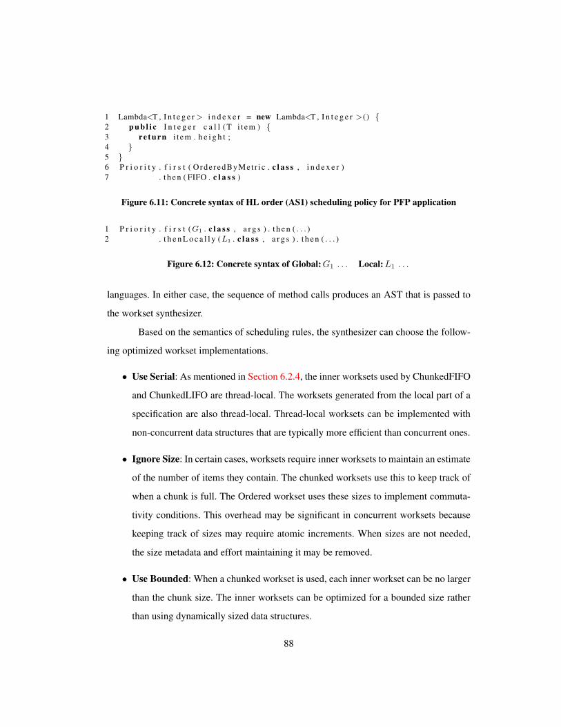
1 Lambda<T , I n t e g e r > i n d e x e r = new Lambda<T , I n t e g e r >() 2 p u b l i c I n t e g e r c a l l ( T i t em ) 3 re turn i t em . h e i g h t ;4 5 6 P r i o r i t y . f i r s t ( OrderedByMet r i c . c l a s s , i n d e x e r )7 . t h e n ( FIFO . c l a s s )

Figure 6.11: Concrete syntax of HL order (AS1) scheduling policy for PFP application

1 P r i o r i t y . f i r s t (G1 . c l a s s , a r g s ) . t h e n ( . . . )2 . t h e n L o c a l l y (L1 . c l a s s , a r g s ) . t h e n ( . . . )

Figure 6.12: Concrete syntax of Global:G1 . . . Local:L1 . . .

languages. In either case, the sequence of method calls produces an AST that is passed to

the workset synthesizer.

Based on the semantics of scheduling rules, the synthesizer can choose the follow-

ing optimized workset implementations.

• Use Serial: As mentioned in Section 6.2.4, the inner worksets used by ChunkedFIFO

and ChunkedLIFO are thread-local. The worksets generated from the local part of a

specification are also thread-local. Thread-local worksets can be implemented with

non-concurrent data structures that are typically more efficient than concurrent ones.

• Ignore Size: In certain cases, worksets require inner worksets to maintain an estimate

of the number of items they contain. The chunked worksets use this to keep track of

when a chunk is full. The Ordered workset uses these sizes to implement commuta-

tivity conditions. This overhead may be significant in concurrent worksets because

keeping track of sizes may require atomic increments. When sizes are not needed,

the size metadata and effort maintaining it may be removed.

• Use Bounded: When a chunked workset is used, each inner workset can be no larger

than the chunk size. The inner worksets can be optimized for a bounded size rather

than using dynamically sized data structures.

88

Ignore Size Use Serial Use Bounded t = 1 t = 8

+ + + 0.0 0.0- + + 0.8 12.1+ - + 2.4 5.5- - + 7.8 7.7+ + - 3.6 3.5- + - 11.3 11.5+ - - 5.0 16.8- - - 2.9 17.5

Figure 6.13: Relative difference in percent (%) of the runtime of PFP application with BASEscheduler on m4x4 machine varying synthesizer optimizations (+: on, -: off) relative to alloptimizations on for one and eight threads

The synthesizer applies rewrite rules over the AST to detect the above cases and

selects, if possible, implementations that are non-concurrent, do not keep track of their size

or are bounded.

To implement these optimizations, the synthesizer introduces new rules (classes) to

represent serial implementations of all the rules and bounded size implementations of the

FIFO, LIFO and Random rules. It also adds an ignore size parameter to each rule, which

determines if the implementation keeps track of its size. Then, the synthesizer traverses

the AST (1) rewriting any rule after a chunked rule to use its serial implementation, (2)

rewriting only rules after an Ordered rule to keep track of their sizes, and (3) rewriting rules

after a chunked rule to use bounded implementations if possible, using the chunk size as

the bound.

Figure 6.13 summarizes the impact of these optimizations for a preflow-push (PFP)

application and a synthesized scheduler called BASE (described in more detail in the fol-

lowing section). Positive numbers indicate how much slower a combination is relative to all

optimizations on. The PFP application was chosen because all the optimizations described

above can be applied and the amount of work done per workset item is small, which in-

creases the relative impact of an efficient workset implementation. From the figure, it is

89

DMR Triangle mesh of 550,000 triangles of which 261,100 are initiallybad

DT 1,733,360 points generated from edge detection of a photographPFP A flow network of 526,904 vertices arranged in 14 consecutive

194x194 frames with uniformly random capacitiesPTA Analysis of the gimp programSSSP Road network of western USA, weights are distances between lo-

cations: 6,262,104 vertices, 15,119,284 edges

Figure 6.14: Datasets used in scheduler synthesis evaluation

clear that these optimizations on worksets have a significant and mostly beneficial impact

on single-threaded and multi-threaded performance.

Evaluation

This section evaluates the scheduler synthesizer on a suite of applications described in Sec-

tion 2.3. Figure 6.14 shows the datasets used for each application. Each application was run

with the following set of schedulers.

• BASE: This is the default scheduler used by the Galois system. It is a synthesized

ChunkedFIFO with a chunk-size of 32.3 Each chunk is a thread-local LIFO.

• FIFO, LIFO, RAND: These schedulers are synthesized from the final rules FIFO,

LIFO and Random. Application-specific schedulers typically use one of these sched-

ulers as their lowest-level (final) scheduler.

• WS-L, WS-F: These schedulers are work-stealing with local LIFOs and FIFOs re-

spectively. These schedulers were ported directly from the Fork-Join implementation

in JSR166 and appear in the Java JDK 7. WS-L is widely used in many parallel sys-

tems.3In the more recent C++ version of Galois, the default scheduler is a distributed chunked FIFO (see Sec-

tion 6.1.1).

90

• BS-L, BS-F: These schedulers use a bulk-synchronous strategy with global LIFOs

and FIFOs respectively. A barrier is used to safely swap between queues concurrently.

• AS1, AS2: These schedulers are synthesized from the application-specific specifica-

tions in Figure 6.8.

The evaluation uses three machines.

• m2x4: a Sun Fire X2270 machine running Ubuntu Linux 8.04.4 LTS 64-bit. It con-

tains two 4-core 2.93 GHz Intel Xeon X5570 (Nehalem) processors. The two CPUs

share 24 GB of main memory. Each core has a 32 KB L1 cache and a unified 256 KB

L2 cache. Each processor has an 8 MB L3 cache that is shared among the cores.

• m4x4: a machine also running Ubuntu Linux 8.04.4 LTS 64-bit. It contains four 4-

core 2.7 GHz AMD Opteron 8384 (Shanghai) processors. Each core has a 64 KB L1

cache and a 512 KB L2 cache. Each processor has a 6 MB L3 cache that is shared

among the cores.

• uma4x8: a Sun T5440 machine running SunOS 5.10. It contains four 8-core 1.4 GHz

Sun UltraSPARC T2 Plus (Niagara 2) processors. Each processor has a 4 MB L2

cache that is shared among the cores.

The Sun JDK v1.6.0 21 was used to compile and run the programs with a heap size

of 20 GB. To control for JIT compilation, each application was run four times within the

same JVM instance and only the last run is reported.

The Galois system uses speculative parallelization (see Section 2.2.1), which intro-

duces overheads from (1) using concurrent implementations of data structures and sched-

ulers rather than their sequential counterparts, (2) acquiring locks to guarantee disjointness

of neighborhoods, and (3) recording undo actions to implement rollback. The serial version

of an application uses sequential data structures only and does not acquire locks or perform

undo actions. The difference in performance between the serial version and the parallel,

91

BASE RAND LIFO FIFO WS-L WS-F BS-L BS-F AS2 AS1

m2x4

DMR 12.88 14.80 11.45 13.09 11.51 13.27 12.76 13.17 15.56 11.62DT 25.04 25.42 14.78PFP 110.93 109.77 169.86 115.40 173.47 116.44 110.18 118.59 45.94PTA 13.87 - - 12.58 - 12.74 20.26 12.84SSSP - - - - - - - - 7.66 4.96

m4x4

DMR 16.29 19.52 13.55 16.76 13.74 16.76 16.25 16.71 19.59 13.64DT 43.40 43.55 27.86PFP 237.04 210.57 320.24 237.17 314.53 234.13 216.50 217.67 74.26PTA 19.99 - - 18.80 - 18.79 26.44 18.82SSSP - - - - - - - - 11.08 9.53

uma4x8

DMR 61.76 68.10 54.79 63.51 53.84 63.31 62.86 64.17 77.81 60.33DT 178.21 179.00 149.42PFP 787.05 734.27 1264.61 741.01 1297.71 775.04 720.20 827.07 342.41PTA 59.17 - - 57.73 - 57.30 76.16 56.99SSSP - - - - - - - - 33.84 23.35

Figure 6.15: Runtimes of serial versions in seconds. In bold are the best serial times, the basisfor the speedup numbers in Figure 6.16. Entries with - timed out. Blank entries indicate invalidor redundant combinations.

one-threaded version is the overhead of enabling speculative execution but never using it.

This overhead can be significant for applications with short activities like PFP and SSSP.

Figure 6.15 shows the runtimes for serial applications. Figure 6.16 shows the par-

allel speedup over the best performing serial scheduler (shown in bold in Figure 6.15). The

runtimes for PTA exclude time to read input, perform offline-cycle detection and write re-

sults. This differs from the methodology of Mendez-Lojo et al., which includes the time

to perform offline-cycle detection (Mendez-Lojo et al., 2010). For all other applications,

runtimes exclude time to read input data or write results but may include sections of the

application that are not parallelized. This portion of time is usually negligible, but for DT

with the AS1 scheduler, this includes time to construct the oct-tree.

92

BASE RAND LIFO FIFO WS-L WS-F BS-L BS-F AS2 AS1

m2x4 (t ≤ 8)

DMR 5.70 4.82 0.95 3.81 4.35 5.13 2.64 3.53 2.01 6.15DT 2.21 2.09 2.35PFP 1.30 0.71 0.20 1.15 0.72 2.30 0.37 0.89 3.35PTA 2.83 - - 3.53 - 2.05 2.37 3.77SSSP - - - - - - - - 0.61 3.16

m4x4 (t ≤ 16)

DMR 7.85 3.43 0.95 3.74 6.94 7.53 1.91 3.83 2.32 10.45DT 2.64 2.65 2.53PFP 1.28 0.62 0.20 1.00 0.65 2.19 0.37 0.74 2.56PTA 3.69 - - 3.63 - 3.08 3.25 5.03SSSP - - - - - - - - 0.80 3.04

uma4x8 (t ≤ 32)

DMR 18.77 5.95 0.89 6.81 11.47 18.53 3.60 5.89 3.59 21.53DT 5.43 5.48 3.29PFP 2.30 1.25 0.32 2.84 2.18 4.46 0.80 2.13 5.92PTA 4.20 - - 4.49 - 5.42 4.62 6.16SSSP - - - - - - - - 0.50 2.33

Figure 6.16: Speedup over serial versions. In bold are the best speedups for each (application,machine) pair. Entries with - timed out. Blank entries indicate invalid or redundant combina-tions.

Empty entries indicate combinations of schedulers and applications that would ei-

ther be redundant or perform significantly worse (by an order of magnitude or more) than

the best serial version. For DT, the performance without randomizing the initial points is

much worse than with randomization. Since the application does not create any new tasks,

the BASE and WS-L runs include an initial timed phase that randomizes the input points.

The other non-random schedulers are omitted because they perform similarly after includ-

ing this phase. For PTA, the RAND, LIFO and WS-L schedulers timed out. For SSSP, only

the AS1 and AS2 schedulers are competitive.

An important result is that the best scheduler for serial execution tends to be the

best for parallel execution as well. This supports the use case where users experiment with

93

BASE RAND LIFO FIFO WS−L WS−F BS−L BS−F AS2 AS1

0.4

0.6

0.8

1.0

4 8 1216 4 8 1216 4 8 1216 4 8 1216 4 8 1216 4 8 1216 4 8 1216 4 8 1216 4 8 1216 4 8 1216Threads

Com

mit

Rat

io

Figure 6.17: Relative number of committed to total iterations for DMR on m4x4

scheduling specifications within a sequential programming model and rely on a synthe-

sis routine to generate efficient, concurrent schedulers that faithfully maintain the desired

scheduling. Also, note the large swings between best and worst schedulers and recall that

the missing entries for PFP, PTA and SSSP correspond to combinations that perform sig-

nificantly worse than the recorded times. Choosing the wrong scheduler can have a drastic

impact on performance.

Overall, the AS1 schedulers perform as well or better than any fixed-function sched-

uler for the same application. Importantly, the BASE scheduler, which is implemented by

a global queue with fixed-size local stacks, performs relatively well across applications.

The DMR application benefits from LIFO policies, while PFP, PTA and SSSP benefit from

FIFO policies.

While direct comparison is not possible, these results are similar to previously

reported results of application-specific schedulers on similar inputs for PFP (Bader and

Sachdeva, 2005), PTA (Mendez-Lojo et al., 2010) and SSSP (Madduri et al., 2006).

Now, let us turn to each application in more detail.

Delaunay mesh refinement Figure 6.15 shows that for the serial implementation, the

best performance is obtained by the LIFO scheduler. When a bad triangle is fixed, it may

create a set of new bad triangles whose cavities overlap with the cavity of the original bad

94

BASE WS−F AS1

0.7

0.8

0.9

1.0

4 8 12 16 4 8 12 16 4 8 12 16Threads

Com

mit

Rat

io

Figure 6.18: Relative number of committed to total iterations for DT on m4x4

triangle. The LIFO scheduler exploits this potential temporal and spatial locality. However,

both of the global LIFO scheduling policies, LIFO and BS-L, perform poorly in a paral-

lel setting because the probability of conflicts increases if triangles close to each other in

the mesh are processed speculatively in parallel. Figure 6.17 shows the relative number of

committed to total iterations on m4x4. The trends are similar for the other two machines.

Not surprisingly, global FIFO schedulers behave the same way. The BASE scheduler, which

uses a global FIFO, ameliorates this problem to some extent by distributing chunks of work

to each thread.

The best performance is obtained with the AS1 scheduler, which is implemented by

a global workset processed in chunked FIFO order and local worksets maintained in LIFO

order. This enables exploitation of locality while controlling the commit ratio, as can be

seen in Figure 6.17.

Delaunay triangulation This application does not create any new work. Its performance

is governed by the initial work order, which should be randomized for best algorithmic

performance. With randomization, the BASE and WS-L schedulers perform similarly. AS1

is significantly faster than the other two schedulers serially, but the performance difference

dissipates as the number of threads increases. Recall that the AS1 scheduler is designed to

increase spatial locality between activities. In speculative parallel execution, this scheduling

95

BASE RAND LIFO FIFO WS−L WS−F BS−L BS−F AS1

1

2

3

4

4 8 1216 4 8 1216 4 8 1216 4 8 1216 4 8 1216 4 8 1216 4 8 1216 4 8 1216 4 8 1216Threads

Rel

. Ite

ratio

ns

Figure 6.19: Relative number of committed iterations to the best performing serial version forPFP on m4x4

strategy causes the commit ratio to decrease, as can be seen in Figure 6.18.

Preflow-push This application is an example of an algorithm whose performance is highly

schedule-dependent because different schedulers result in dramatically different amounts of

work. Figure 6.19 shows the number of iterations committed relative to the best performing

serial version on m4x4. Most schedulers result in twice as many iterations as the best serial

version. LIFO and WS-L perform four times more iterations in some cases. Figure 6.15

shows the impact of the varying work on the serial versions. The runtime of the fastest and

slowest schedulers differ by a factor of more than three.

For a hand-parallelized implementation of PFP using the heuristics described in

Section 2.3, Bader and Sachdeva reported a maximum speedup of about 2 with eight pro-

cessors on an UltraSPARC II architecture with an input similar to that used here, which is

referred to as an RMF graph (Bader and Sachdeva, 2005).

Inclusion-based points-to analysis This application is another example of a highly sched-

ule-dependent algorithm. The PTA application performs a fixpoint computation, and for

these computations, FIFO policies usually perform well because a variable gets to accu-

mulate several updates before its value is propagated down-stream. LIFO policies perform

96

poorly, and most versions time-out. BS-F, which alternates between two queues, does the

best on this input. However, on other inputs, not shown here, BASE outperforms BS-F.

As noted earlier, these results are based on the implementation of Mendez-Lojo et

al., the first parallel implementation of PTA (Mendez-Lojo et al., 2010).

Single-source shortest-Path This application is a case where the generally accepted best

serial scheduler, which is AS2 and is based on Dijkstra’s algorithm, does not perform well

in parallel. It has better theoretical algorithmic complexity, but the concurrent priority queue

limits performance on most inputs. The difficulty in implementing such queues is one moti-

vation for the delta-stepping order (AS1), which seeks to balance good order with efficient

concurrent implementation. From experiments not shown here, it can be shown that the

delta-stepping order performs only 1.2 times more work than Dijkstra’s algorithm for this

input, an overhead that is modest enough to overcome through parallelism.

Madduri et al. produced an implementation of delta-stepping for the Cray MTA-2

architecture (Madduri et al., 2006). On the same input used here, a road network of the

western USA, they reported a maximum speedup of about 2 on sixteen processors.

6.3 Exploiting Data Locality

Locality is exploited in the Galois system by scheduling activities according to the physical

layout of data structures.

Although Galois data structures present a single logical view of data, they are often

physically partitioned by thread or by package or by NUMA node. For instance, the morph

graph described in Section 5.5 has nodes partitioned by thread. Users are not exposed to

this partitioning directly, but through a scheduling policy, they can request that active nodes

be initially assigned to the thread that owns the corresponding data. This increases the

locality when the neighborhood of an operator is just the active node, which is common in

data-parallel loops. Since partitions may be unbalanced, once a thread runs out of active

97

netflix yahoo

0

25

50

75

100

125

10

20

30

40

20 40 20 40Threads

GF

LOP

S

Kind galois graphlab nomad

Figure 6.20: Throughput of matrix completion operators on machine m4x10 (theoretical peakthroughput: 363.2 GFLOPS)

nodes that it owns the data for, it uses workstealing to find new work corresponding to

other threads’ partitions. In this way, locality can be exploited but full thread utilization is

preferred over working on non-local data.

When neighborhoods consist of multiple nodes of a partitioned data structure, it

is not obvious in general how to assign active nodes to threads. The owner-computes rule

is one such strategy (Rogers and Pingali, 1989). For maximum effectiveness, the neigh-

borhood of an operator should be contained to a single partition. Space-filling curves can

be applied for geometric graphs, and graph partitioning algorithms (Karypis and Kumar,

1997) can be applied to arbitrary sparse graphs to increase the likelihood that a node’s

neighbors are assigned to the same partition, but general graph partitioning algorithms can

be expensive relative to simple graph analytics algorithms. The well-known Metis graph

partitioner can be expressed and parallelized in the Galois system (Sui et al., 2011), which

raises the possibility of exploiting locality for more heavyweight algorithms. Recently more

lightweight matrix reordering algorithms have been implemented in Galois (Karantasis

98

13 32263

netflix

0.9

1.1

1.3

1.5

0 50 100 150 200Time (s)

Err

or

331333

yahoo

17.5

20.0

22.5

25.0

27.5

30.0

0 200 400 600Time (s)

Err

or

Kind galois graphlab nomad

Figure 6.21: Convergence of matrix completion with 20 threads on machine m4x10. Horizontalline indicates error threshold of 90% of minimum observed error. Numbers indicate time toreach threshold.

et al., 2014), which also can be used to increase the likelihood that the neighborhood of

an activity is localized to a small region of the physical data structure. Since the Galois

system provides parallel data structures and scheduling, integrating these reordering and

partitioning algorithms should not require significant changes in user programs, but a com-

prehensive solution has not yet been implemented.

Some locality optimizations can be framed as different scheduling policies. As an

example, consider the matrix completion problem described in Section 2.3. When using

SGD, the operator is over an edge and its two endpoints in a bipartite graph. In practice, the

data associated with each endpoint is a reasonably sized vector (k ≈ 100), which means

that a high locality schedule is one that assigns edges to threads in such a way that the edges

assigned to a thread share as many endpoints as possible. In this way, activities on edges

reuse node data as much as possible. If the graph were complete, this schedule would re-

semble classical tiling for matrix-matrix multiply. However, in this case, the graph is sparse

and the operator writes to its endpoints, which means that activities that share endpoints

cannot be scheduled concurrently.

99

That being said, this sparse tiling is still a useful optimization. Figure 6.20 shows the

computational throughput of SGD for matrix completion on two inputs, netflix (17 K items,

480 K users, 99 M ratings) and yahoo (624 K items, 1 M users, 253 M ratings). The label

Galois refers to an application in Galois using sparse tiling, which is simply a scheduling

policy applied to the basic SGD algorithm; GraphLab refers to an application written in the

GraphLab parallel programming model and does not do any locality optimizations; Nomad

is a hand-written parallel code using MPI and pthreads (Yun et al., 2014). It tries to reduce

communication (increase locality) by cyclically scheduling block diagonals of the matrix

representation of the bipartite graph. The results show that even the simple block diagonal

tiling done by Nomad is a significant improvement over no tiling at all and that the sparse

tiling implemented in Galois can provide further performance improvements.

Figure 6.21 shows the impact of the improved throughput on the end-to-end com-

putation which runs until a certain error level is reached or for a certain amount of time. In

this case, there are additional randomization steps taken by the Nomad implementation that

reduce the initial throughput advantage of the Galois implementation for the yahoo input

as time goes on, which is why 50% throughput improvement does not translate into a 50%

reduction in overall time.

6.4 Coordinated Scheduling

The discussion so far has focused on autonomous scheduling (see Section 2.2.3), where

activities are scheduled without global communication. Coordinated scheduling, where ac-

tivities are executed in bulk-synchronous rounds, is also possible in the Galois system. An

accumulating collection is a collection of elements that supports concurrent insertion of

new elements but does not need to support concurrent reads of the collection. Coordinated

scheduling policies can be built from multiple autonomously scheduled loops and an ac-

cumulating collection data structure, which is provided by the Galois library. For example,

loop 1 executes, populating a collection with work that should be done by loop 2. Then,

100

loop 1 finishes, and loop 2 iterates over the collection generated by loop 1, and so on.

Control logic can be placed between loops, allowing the expression of sophisticated coor-

dinated strategies like the pull versus push operators required for breadth-first search (see

Section 2.3).

6.5 Related Work

Although the Galois system synthesizes schedulers from specifications, this is not the stan-

dard concurrent program synthesis problem considered in the literature (Vechev et al., 2007;

Solar-Lezama et al., 2008). Scheduling specifications for unordered algorithms are inher-

ently “fuzzy” (even FIFO scheduling of the workset can result in different executions de-

pending on the speed of processors). Therefore, a scheduling specification is advice to the

runtime system about how to bias scheduling decisions for efficiency, whereas in conven-

tional program synthesis, implementations must satisfy specifications exactly.

Some work has shown that more efficient workset implementations may be possible

if the application is written so that it can tolerate duplicate work items (Michael et al., 2009;

Leijen et al., 2009). Exploiting this idempotence property would require changes to the def-

initions in Section 6.2 and Section 6.2.1, but the implementation would be straightforward

for final worksets. However, some non-final worksets, such as the chunked worksets, de-

pend on the correspondence between adds and polls, which makes taking advantage of

idempotence a challenge in these cases.

Previously, Kulkarni et al. (Kulkarni et al., 2008) explored different handwritten

scheduling policies in the Galois system. However, the policies were a small number of

fixed forms. In contrast, the schedulers described here are synthesized (not handwritten),

they include policies studied in the literature such as delta-stepping, and they can be com-

posed arbitrarily, which is important in practice.

There are several concurrent priority queues implementations (Hunt et al., 1996;

Shavit and Lotan, 2000; Sundell and Tsigas, 2005; Bronson et al., 2010). Preliminary

101

studies using concurrent skip-lists (Shavit and Lotan, 2000), a common implementation,

revealed poor performance in the Galois system. Improved performance can be achieved

by using bounded priorities (Shavit and Zemach, 1999), but the basic problem of lack of

scalability remains. Chazelle investigated approximate priorities (Chazelle, 2000) but only

considered sequential implementations.

Another possibility is to use a concurrent priority queue for each thread with work-

stealing from other priority queues if the local priority queue becomes empty. Variations of

this idea have been used previously in the literature (Papaefthymiou and Rodrigue, 1994;

Bertsekas et al., 1996), and it is also used in GraphLab (Low et al., 2010). However, the

work efficiency of the resulting implementation is often poor because early priority work

generated by one thread does not diffuse quickly enough to other threads.

Yet another possibility is to use a concurrent priority queue for each thread, with

logically partitioned graphs and the owner-computes rule (Rogers and Pingali, 1989) for

task assignment. When task a creates a new task b, it looks at the partition assigned to task

b to determine which priority queue to push task b on. This policy is used in GraphLab

and other systems (Tang et al., 2008; Pearce et al., 2010). This policy is well-suited for

distributed systems and has been used in distributed graph traversal algorithms (Pearce

et al., 2010) but will perform poorly when work is localized to a subset of partitions.

102

Chapter 7

Deterministic Scheduling

In the optimistic scheduling described in Chapter 6, when there is a conflict between two

tasks1, there is no particular order in which those tasks are executed, which can result in

non-deterministic program execution. Non-deterministic scheduling is sufficient for many

applications, but it is also possible to use a deterministic scheduler to guarantee that task

conflicts are resolved in a reproducible way if desired.

The way non-determinism appears in the operator formulation is as follows:

• P is a pool of tasks that can be performed in any order, i.e., an unordered algorithm.

The program terminates when all tasks have been executed.

• When task t is completed, it may create a set of new tasks S(t), which are added to

the task pool. Task t is the parent of the tasks it creates; the transitive closure of the

parent relation is called the ancestor relation.

• Each task performs computation and reads and writes shared-memory locations. The

set of locations read R(t) and written W (t) by a task t is said to constitute its neigh-

borhood, which is denoted by L(t) = R(t)∪W (t). Tasks are required to be cautious:

This chapter draws from (Nguyen et al., 2014), where deterministic scheduling for the Galois system wasoriginally described.

1This chapter uses task interchangeably for activity to emphasize the applicability of these techniques forall programs including those not written in the operator formulation.

103

that is, a task must read all of the locations in its neighborhood before it can write to

any of them.

• A conflict occurs between tasks t1 and t2 if (1) neither task is an ancestor of the other,

and (2) one of them writes to the neighborhood of the other (W (t1) ∩ L(t2) 6= ∅).

If there can be no conflicts between tasks, parallel execution is straightforward since

the program is a generalized data-parallel loop in which the iteration range can grow

dynamically. In the presence of conflicts, a correct parallel schedule for the program

should be serializable: it must appear as if all tasks were performed atomically in

some order that respects the ancestor relation.

Non-determinism arises in this formulation because the serialization order between

conflicting tasks is not defined. Schedulers that guarantee the same serialization order be-

tween conflicting tasks are deterministic. In practice, there may be other sources of non-

determinism in the system, e.g., the tasks themselves use random variables or read non-

deterministic external state; in this chapter, we will restrict ourselves to systems where the

only source of non-determinism is the order in which conflicting tasks execute.

Section 7.1 outlines a method of deterministically scheduling any unordered algo-

rithm, but it requires runtime analysis to deal with potentially changing runtime depen-

dencies. Under certain program restrictions, this deterministic runtime scheduling can be

refined to use more efficient schedulers (see Section 7.2).

7.1 Interference Graph Scheduling

One general deterministic scheduling technique is based on successive construction and

scheduling of interference graphs.

Definition 7.1. Given a set of tasks P , an interference graph for P is an undirected graph

GP = (VP , EP ) in which there is a distinct node in VP representing each task in P , and

104

there is an undirected edge (v1, v2) ∈ EP if the tasks represented by v1 and v2 have a

conflict.

The interference graph for a set of tasks can be built by executing each task up to its

failsafe point (see Section 2.2.1) while tracking its neighborhood and putting a conflict edge

between two tasks if their neighborhoods overlap. This is a conservative approach since it

puts a conflict edge between two tasks even if they both read a location that neither of them

writes to. A more precise technique which distinguishes reads from writes is described later

in Section 7.1.2.

Interference graphs can be used to schedule tasks as follows. The tasks in the task

pool P are executed in rounds. In each round, the scheduler performs the following activi-

ties:

• inspect: builds an interference graph GP for the tasks in P ,

• select: finds an independent set I of nodes in GP and removes the corresponding

tasks from P , and

• execute: executes the tasks in I in parallel, adding any newly created tasks to P .

Scheduling is completed when all tasks have been executed. During the select phase,

it is desirable but not necessary to find a maximal independent set of nodes in the graph.

A subtle point is that the interference graph must in general be rebuilt from scratch

each round since the neighborhood of a task is relative to the global state, which is modified

by tasks in the execute phase. For instance, consider three tasks: task t1, which writes 1 to

location l1; task t2, which reads l1 and if it is 1, writes to l2 otherwise it does nothing; and

task t3, which reads from l2. Let the initial value of l1 be 0. The initial interference graph

is G0P = (V 0

P = vt1 , vt2 , vt3, E0P = (vt1 , vt2)). Assume that only task t1 executes. In

the following round, the interference graph is G1P = (V 1

P = vt2 , vt3, E1P = (vt2 , vt3)).

Note that the edge between vt2 and vt3 only appears after executing task t1.

105

1 Tasks cur , nex t , t odo2 todo = P ;3 whi le | | t odo | | > 0 :4 / / o r d e r t a s k s i n todo d e t e r m i n i s t i c a l l y5 n e x t = s o r t ( t odo )6 todo = 7 / / e x e c u t e s o r t e d t a s k s8 whi le | | n e x t | | > 0 : / / f o r each round . . .9 ca l cu l a t eW indow ( )

10 b a r r i e r . w a i t ( )11 / / g e t p r e f i x o f s i z e window from n e x t12 cur , n e x t = getWindowOfTasks ( n e x t )13 / / compute n e i g h b o r h o o d s o f t a s k s i n cur14 i n s p e c t ( c u r )15 b a r r i e r . w a i t ( )16 / / e x e c u t e s u c c e s s f u l t a s k s , move17 / / f a i l e d t a s k s t o nex t , and add any18 / / newly c r e a t e d t a s k s t o todo s e t19 todo = todo ∪ s e l e c t A n d E x e c ( cur , n e x t )20 b a r r i e r . w a i t ( )

Figure 7.1: Deterministic scheduler

There is an enhancement to this basic scheme that is useful for reducing the over-

head of interference graph construction. Note that the scheduling strategy works correctly

even if, in each round, the interference graph is constructed only for a subset of tasks in

the pool; the remaining tasks are simply delayed to later rounds. This windowing scheme

can reduce the overhead of interference graph construction when the number of tasks is

much larger than the number of threads because the conflict rate monotonically increases

with the number of tasks inspected a round. For the windowed scheduler to be determin-

istic, one must ensure the following in each round: (1) tasks for the current window are

chosen deterministically from the task pool, and (2) during the select phase, the indepen-

dent set of nodes is chosen deterministically. Section 7.1.1 describes an implementation of

deterministic interference graph (DIG) scheduling.

106

1 Tasks s o r t ( Tasks todo ) :2 / / s o r t t a s k s i n s e t t odo34 void i n s p e c t ( Tasks c u r ) :5 d o a l l t in c u r :6 wri teMarksMax ( i d ( t ) , L ( t ) )78 Tasks s e l e c t A n d E x e c ( Tasks cur , Tasks n e x t ) :9 Tasks newWork =

10 d o a l l t in c u r :11 i f readMarks (L ( t ) ) == i d ( t ) :12 / / a l l r e a d s e q u a l id , so e x e c u t e t a s k t13 t ( )14 / / add new work i f any t o newWork15 newWork = newWork ∪ S ( t )16 e l s e :17 n e x t = n e x t ∪ t18 w r i t e M a r k s ( i d ( t ) , 0 , L ( t ) )19 re turn newWork2021 bool w r i t e M a r k s ( Id expec t ed , Id id , Set<Loc> l o c s ) :22 f o r l o c in l o c s :23 atomic :24 i f Mark ( l o c ) == e x p e c t e d :25 Mark ( l o c ) = i d26 e l s e :27 re turn f a l s e28 re turn true2930 void writeMarksMax ( Id id , Set<Loc> l o c s ) :31 f o r l o c in l o c s :32 atomic :33 i f Mark ( l o c ) < i d :34 Mark ( l o c ) = i d3536 Set<Id> readMarks ( Set<Loc> l o c s ) :37 / / r e t u r n s e t o f i d s i n mark l o c a t i o n s

Figure 7.2: Auxiliary functions for deterministic scheduler

107

7.1.1 Deterministic Interference Graph Scheduling

Figure 7.1 shows the pseudocode for the implementation of deterministic scheduling; aux-

iliary functions are shown in Figure 7.2. In the pseudocode, doall indicates a loop whose

iterations are run in parallel. Instead of explicitly building an interference graph, this code

directly finds an independent set of tasks by using marks on locations.

A summary of what the scheduler does is the following. The task set todo is initial-

ized to the initial set of tasks P. These tasks are ordered deterministically to form a sequence

next. This sequence of tasks is executed over several rounds; in each round, a prefix cur of

tasks in next is tried for execution. Some of these will succeed and others may fail. Tasks

created by successful tasks are added to todo; these are executed after next becomes empty.

Failed tasks are added back to next and retried in later rounds. Execution terminates when

todo and next become empty.

The inspect operation uses writeMarksMax to mark the neighborhood of a task,

stealing ownership of neighborhood locations from tasks with lower ids. While the mark on

a given location may be updated non-deterministically depending on how the tasks in cur

are scheduled, the final mark values will be the same regardless of the order in which tasks

were processed in the inspect phase. This is because the maximum (or minimum) element

of a set with a total order is deterministic (the set in question is the set of ids of the tasks

that read or wrote to a particular location in the current round).

The non-deterministic Galois execution uses exclusive locking (see Section 5.2)

to identify conflicts. The behavior of exclusive locking is like the writeMarks function

in Figure 7.2. One important difference between writeMarks and writeMarksMax is that

writeMarks can fail early if it cannot update a mark location, but in order to be determin-

istic, writeMarksMax must attempt to update all mark locations even if it failed to update

some of them. If a task skips some mark locations, it changes the set that writeMarksMax

is computing the maximum of, and if the mark locations skipped depend on a scheduling

choice, then the resulting maximums are non-deterministic.

108

In the second phase, the scheduler selects and executes an independent set of tasks

(line 19 in Figure 7.1 and function selectAndExec in Figure 7.2). A task is selected if all

of its neighborhood locations are still marked with its id at the end of the inspection phase.

Tasks selected this way form an independent set in the interference graph. This set is unique

because of the total order on ids. If any of the neighborhood locations of a task does not

contain its id, the task is not part of the independent set, and it is placed in the next set

to be executed in a future round. In either case, the marks written by a task are cleared in

preparation for the next round.

Execution continues in rounds until there are no tasks left in next. If there are no

tasks in the todo set, the scheduler terminates; otherwise these tasks are moved to next, and

execution continues. Note that in each round, the task in cur with maximum id is guaranteed

to execute, so each round executes at least one task.

Before enqueued tasks can be scheduled, they must be assigned a unique id. The

assignment of ids must also be deterministic. Ids are assigned as follows. The initial tasks

are given ids based on the iteration order of the C++ iterator that contains the tasks. When

task t creates task u, the scheduler stores with task u the id of the task that created it id(t)

and a number k indicating whether it was the first, second, third, etc. task created by t. In

the sort function, tasks are sorted lexicographically based on the pair (id(t), k), and the

scheduler uses the position in the total order defined by the sort as the id for the new tasks.

The performance of this scheduler depends critically on the window size, so the

scheduler uses an adaptive algorithm that grows and shrinks the window size each round

depending on the number of tasks that successfully committed in the previous round. The

getWindowOfTasks and calculateWindow functions in Figure 7.1 implement this function-

ality. The calculateWindow function computes the window size for the current round based

on the fraction of tasks that committed in the previous round. If the commit ratio is less than

some target threshold (0.95 in these experiments), the next window size is scaled down pro-

portionally. If the commit ratio is above the threshold, the window size is doubled. The

109

getWindowOfTasks function simply returns this prefix of tasks in cur and postpones the

remainder to next. Since the number of tasks that commit in a round is independent of the

number of executing threads, this heuristic is portable across machines.

To implement the deterministic marking scheme in the Galois system, there are two

changes that need to be made to the non-deterministic scheduling system.

First, the default mark values in the Galois system are not ordered. The marking

code needs to be modified to keep track of the id of a task and to use that value appropriately

when writing mark values.

Second, neighborhoods are not explicitly maintained by the Galois system. Marks

are acquired incrementally during execution via user code calls to a data structure library.

The only way to get the neighborhood of a task is to execute the task and observe which

marks are acquired. To implement the inspect phase, tasks are simply executed, which,

by their normal execution, mark locations in their neighborhoods. When a task reaches its

failsafe point (the first write to a global location), it immediately returns. To implement

the selectAndExec phase, tasks are re-executed from the beginning, and instead of writing

marks, they check whether the marks that would have been written match the values that

have been written. This implements line 11 of Figure 7.2. If a task reads a mark value that

is not its id, the scheduler goes to line 17.

This baseline implementation is sufficient to deterministically schedule any un-

ordered algorithm in the operator formulation.

7.1.2 DIG Optimizations

The baseline deterministic scheduler described in Section 7.1.1 contains several inefficien-

cies, which are addressed in an optimized scheduler.

First, it redundantly executes the prefix of a task up to its failsafe point when a task

is selected and executed. A more efficient method would be to suspend execution of a task

at the failsafe point during the inspect phase and to resume execution in the commit phase.

110

On resumption, the task must check that all the mark values still match its id (Figure 7.2

line 11). The capability to pause and resume execution can be achieved generally using

additional threads or creating continuations. The optimized scheduler uses a more ad-hoc

approach, which simulates the effect of forming a continuation without implementing a full

compiler transform. The scheduler provides a library function that allows users to allocate

objects in the inspect phase which can be recalled during the commit phase. Programmers

can use this functionality to manually achieve the same effect as task suspend and resume.

To make sure that resumed tasks are valid to commit, the optimized scheduler makes

a small change to the protocol in the inspect phase. Instead of just writing the maximum

mark value, a task t checks if the previous value of the mark location is not 0 and not

id(t); if so, by writing its mark, task t will prevent the task u that corresponds to the current

mark value from committing. Normally, task u detects this case when the scheduler executes

line 11, or in the case of the baseline scheduler, when task u is executed a second time. When

using the continuation optimization, t is now responsible for preventing u from executing.

It does this by writing to a flag variable that u checks before resuming execution.

Second, the performance of the scheduler is very sensitive to initial task order. Ap-

plications that exploit temporal locality execute tasks with overlapping neighborhoods close

in time. This typically translates to those tasks being close together in iteration order, which,

in the baseline scheduler implementation, means that they typically will be executed in the

same round, where they will certainly conflict with each other. This leads to the perverse sit-

uation where the scheduler needs to reduce locality to improve performance. The optimized

scheduler addresses this issue by assuming that tasks placed close together in iteration order

have high locality and places those tasks in separate rounds if possible.

Third, the cost of sorting enqueued tasks can be large relative to the application

time. There is a common special case where a task enqueues tasks, but those tasks are

drawn from a fixed set of tasks. In this case, tasks can be assigned unique ids before parallel

execution, and the programmer can pass these ids to the scheduler, which uses them directly

111

instead of generating new ids via the sort function.

Two possible optimizations not yet included in the optimized scheduler are the fol-

lowing.

First, instead of sorting tasks to generate ids for enqueued tasks, any deterministic

hash function can be used instead. One way to generate unique ids with a deterministic

hash function is to use a variation of linear probing with priority writes (Shun and Blelloch,

2014).

Second, the interference graph has an edge whenever two tasks have overlapping

neighborhoods, but if both tasks only read locations the overlapping region, these tasks can

be allowed to proceed in parallel. This situation does not frequently occur in the applications

evaluated in Section 7.1.3, but allowing such tasks to proceed in parallel only requires a

small modification to the deterministic interference graph scheduling algorithm. Each task

t now has two ids, wid(t) which is the id it marks when it wants to write to a location, and

rid(t) which is the id it marks when it wants to read a location. Marking a location to write

is the same as before. When marking a location to read and the previous owner is a write

id, the behavior is the same as a write. When marking a location to read and the previous

owner u is a read id, the task t updates a disjoint-set data structure to record that t and u

both have a read dependency on the same location. After the inspect phase, another phase

is added to check if any location read was subsequently marked by a writer, and if so, the

tasks that have a read dependency on that location are disabled for the current round. To

ensure progress, the read and write id the greatest task (in a window) should be greater than

the read and write ids of any other task.

Even with these implemented and proposed optimizations, there are some inherent

inefficiencies that are introduced by any DIG scheduling implementation compared to non-

deterministic scheduling.

1. The deterministic scheduler executes many more instructions than non-deterministic

scheduling.

112

2. The deterministic scheduler introduces a concept of rounds that is not present in

the original program. These rounds are implemented using global synchronization.

Rounds extend the critical path length of a program because the scheduler cannot

proceed to the next round until all of the tasks are processed for the current round.

3. The scheduler executes tasks according to a particular schedule, but that schedule

may not be the best performing one among possible program schedules.

4. The execution of a task is broken into two parts, the inspect phase and the execu-

tion phase, separated by a barrier. The memory locations accessed during the inspect

phase of a task are very likely to be accessed by the execution phase of the same

task, but under DIG scheduling, these two phases are temporally separated by a fac-

tor that is a function of number of tasks attempted during a round, which is typically

very large. Conversely, increasing locality by reducing the number tasks attempted

in a round increases the number of rounds executed, which increases the critical path

length of the program.

7.1.3 Evaluation

To evaluate DIG scheduling, applications were drawn from three different sources: the

PARSEC (v2.1) benchmark suite (Bienia et al., 2008), the problem based benchmark suite

(PBBS) (v0.1) (Blelloch et al., 2012), and the Lonestar (v2.1.5) benchmark suite (Kulkarni

et al., 2009).

The PARSEC benchmark suite has been used in previous evaluations of determinis-

tic scheduling (Bergan et al., 2010a; Devietti et al., 2011; Liu et al., 2011). It contains twelve

applications or kernels. Most are parallelized using the pthread library. The evaluation uses

the three benchmarks that have OpenMP implementations: blackscholes, bodytrack and

freqmine. The blackscholes and freqmine results are for the simlarge input, while the body-

track results are for the native input.

113

The PBBS programs (Blelloch et al., 2012) are organized by problem, and each

problem has one or more solution programs, at least one of which is deterministic. There

are a total of sixteen problems, but many of these programs are data-parallel or nested

data-parallel, and their performance depends largely on factors like good load balancing

and not on scheduling and therefore were excluded from this evaluation. The remaining

deterministic programs solved the five remaining problems: breadth-first search (BFS), De-

launay triangulation (DT), Delaunay mesh refinement (DMR), maximal independent set

(MIS), and maximal matching. Maximal matching was excluded from the evaluation due

to its similarity to maximal independent set. In these codes, determinism is ensured by

application-specific techniques customized to each application, and they typically involve

bulk-synchronous execution in rounds. The PBBS maximal independent set program is

data-parallel, but it is included in this evaluation for comparison with a non-deterministic

maximal independent set program that exists in the Lonestar suite.

From the Lonestar benchmark suite, the evaluation contains four programs that

solve the same problems as those included from PBBS, using the same algorithms, and an

implementation of the preflow-push algorithm (PFP) that uses the global relabeling heuris-

tic to improve convergence (see Section 2.3). The deterministic implementations of all Lon-

estar programs are automatically generated by applying the DIG scheduler (Section 7.1.1)

and its optimizations (Section 7.1.2).

There is one small difference between the PBBS and Lonestar implementations of

Delaunay triangulation. The algorithmic complexity of Delaunay triangulation depends on

the order in which points are inserted, and random insertion order has been shown to be

optimal (Clarkson and Shor, 1989). In the PBBS implementation, points are randomized

offline. In the Lonestar implementation, points are reordered online using the biased ran-

domized insertion order algorithm (Amenta et al., 2003). For comparison purposes, the

evaluation does not include the reordering time in either implementation.

The performance of the PBBS and Lonestar benchmarks can vary significantly with

114

the type of input. From experience, the behavior across random inputs for an application

is largely similar, so the evaluation uses a single representative input for each application.

These inputs are largely drawn from the evaluation of Blelloch et al. (Blelloch et al., 2012).

The BFS results use a random graph of 10 million nodes where each node is connected to

five randomly selected nodes. The DMR results use a Delaunay triangulated mesh of 2.5

million randomly selected points from the unit square. The DT results use 10 million points

randomly selected from a unit square. The MIS results use the same input as BFS. The PFP

results use a random graph of 223 nodes with each node connected to 4 random neighbors.

In the experimental results, the variant g-n denotes the original non-deterministic

Lonestar application, and the deterministic variant generated from DIG scheduling is called

g-d. The variant PBBS denotes the PBBS version of the application.

The evaluation uses three machines and runtimes are the average of at least three

runs for each application/machine/thread-count combination. The three machines are

1. m4x10, a machine running Ubuntu Linux 10.04 LTS 64-bit (Linux 2.6.32) with four

ten-core Intel Xeon E7-4860 (2.27 GHz) processors;

2. m4x6, a machine running Ubuntu Linux 10.04 LTS 64-bit (Linux 2.6.32) with four

six-core Intel Xeon E7540 (2.0 GHz) processors; and

3. numa8x4, an SGI UV machine (ccNUMA) running SuSE Enterprise 11 SP1 64-

bit (Linux 2.6.32.24) with eight four-core Intel E7520 (1.87 GHz) processors. The

processors of numa8x4 are divided into blades of two processors each and enclosures

of two blades each. Inter-blade communication uses SGI NUMALink 5.

Programs are compiled with icc version 12.1 with the -O3 optimization flag. For

the PBBS programs, the Cilk runtime is used to manage and load balance threads. For the

Lonestar programs, the Galois runtime system is used.

The evaluation is divided into four parts.

115

1. The first part (Application Characteristics) describes applications characteristics use-

ful for understanding the performance results.

2. The second part (Deterministic Thread Scheduling) compares the performance of

non-deterministic programs with and without CoreDet (Bergan et al., 2010a), a sys-

tem that provides determinism by modifying how threads are scheduled. Because the

C++ language primitives used in the Lonestar programs are not supported by Core-

Det, the evaluation uses non-deterministic versions of the PBBS programs as repre-

sentative of the non-deterministic benchmarks. The evaluation shows that with Core-

Det, the non-deterministic PBBS programs do not perform well and have a median

slowdown of 3.7X (min: 1.3X, max: 55X) compared to running without CoreDet.

These experiments show that systems like CoreDet that provide determinism through

deterministic thread scheduling are not suitable for irregular applications, which have

relatively fine-grain tasks.

3. The third part (DIG Scheduling) compares the performance of non-deterministic Ga-

lois programs (g-n), generated deterministic implementations of these Galois pro-

grams (g-d), and handwritten deterministic PBBS programs for the same problems.

Overall, the results show that at the maximum number of threads on each machine,

(1) g-n variants achieve a median improvement of 4.2X compared to g-d, (2) g-n

variants are 2.4X faster than the PBBS variants, and (3) g-d variants are only 0.62X

slower than the PBBS variants.

4. These results show that the automatically generated deterministic Galois programs

are comparable in performance to the handwritten PBBS programs and that there

is a significant performance penalty for deterministic execution. Finally, a study with

performance counters (Determinism and Locality) reveals that, for the most part, non-

deterministic programs perform better than deterministic ones because they exploit

more locality.

116

p = 1 p = 40

AbortRatio

Tasksper µs

AbortRatio

Tasksper µsVariant Rounds

bfs g-d 1700 0.08 0.45 0.08 9.76bfs g-n 0 0 1.32 0 39.92bfs pbbs 11 0 1.24 0 24.27

dmr g-d 1287 0.11 0.13 0.11 2.53dmr g-n 0 0 0.26 < 0.01 8.98dmr pbbs 1165 0.03 0.18 0.03 2.90

dt g-d 35213 0.27 0.12 0.27 1.78dt g-n 0 0 0.24 < 0.01 7.47dt pbbs 1330 0.10 0.11 0.10 2.48

mis g-d 100 0.08 0.77 0.08 21.05mis g-n 0 0 3.98 < 0.01 79.69mis pbbs 29 0.05 14.59 0.05 143.12

pfp g-d 21047 0.04 0.26 0.04 2.58pfp g-n 0 0 0.67 < 0.01 14.99

Figure 7.3: Abort ratio and task execution rates on machine m4x10

Application Characteristics

Previous evaluations of deterministic scheduling have focused mostly on applications with

coarse-grain tasks that communicate relatively infrequently. Deterministic scheduling for

these kinds of applications can be supported using relatively heavyweight mechanisms

since the overhead of the system is a small fraction of the overall execution time. How-

ever, these mechanisms may not be useful for applications with very lightweight tasks that

communicate frequently. On a shared-memory system, the concept of communication is

less well-defined compared to a distributed system, but one approximation is the number

of atomic updates an application performs. Figure 7.3 shows task execution rates and abort

ratios on machine m4x10 with 1 and 40 threads. Figure 7.4 shows atomic update rates. For

117

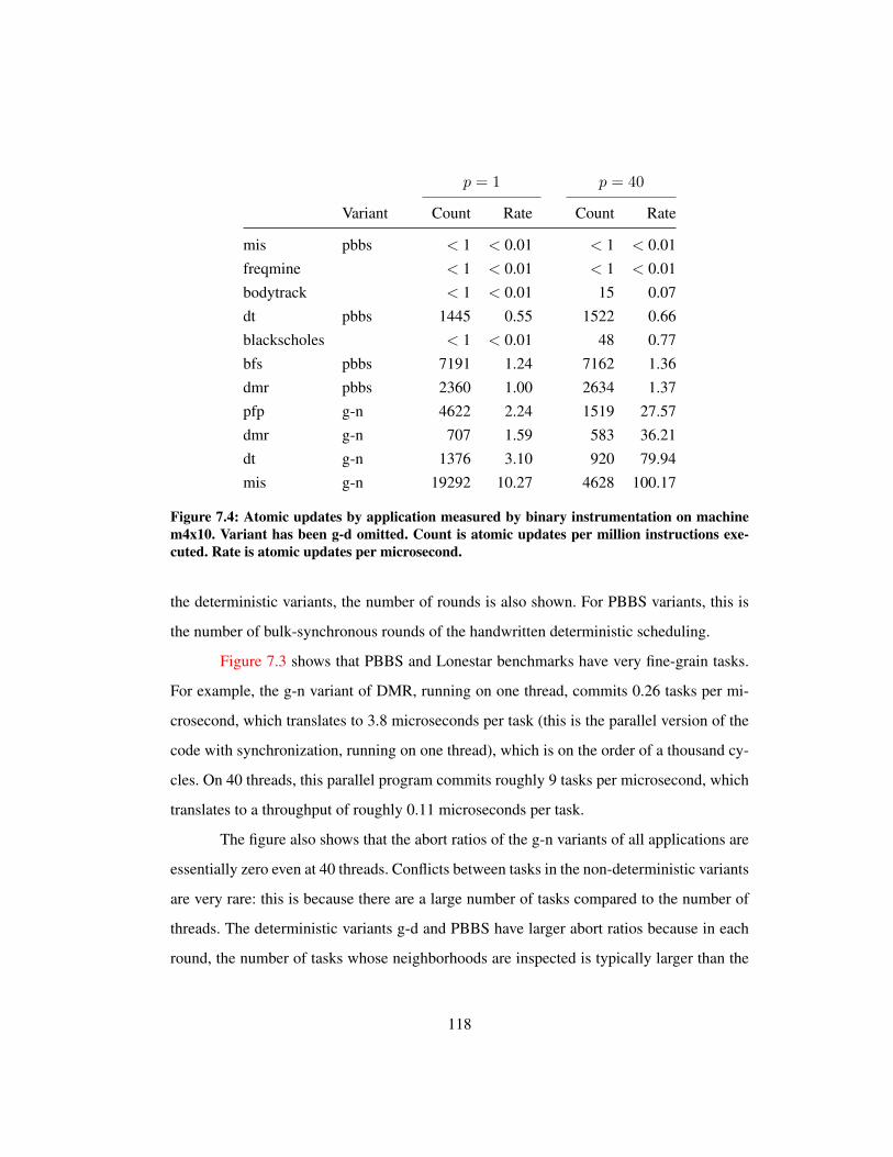
p = 1 p = 40

Variant Count Rate Count Rate

mis pbbs < 1 < 0.01 < 1 < 0.01freqmine < 1 < 0.01 < 1 < 0.01bodytrack < 1 < 0.01 15 0.07dt pbbs 1445 0.55 1522 0.66blackscholes < 1 < 0.01 48 0.77bfs pbbs 7191 1.24 7162 1.36dmr pbbs 2360 1.00 2634 1.37pfp g-n 4622 2.24 1519 27.57dmr g-n 707 1.59 583 36.21dt g-n 1376 3.10 920 79.94mis g-n 19292 10.27 4628 100.17

Figure 7.4: Atomic updates by application measured by binary instrumentation on machinem4x10. Variant has been g-d omitted. Count is atomic updates per million instructions exe-cuted. Rate is atomic updates per microsecond.

the deterministic variants, the number of rounds is also shown. For PBBS variants, this is

the number of bulk-synchronous rounds of the handwritten deterministic scheduling.

Figure 7.3 shows that PBBS and Lonestar benchmarks have very fine-grain tasks.

For example, the g-n variant of DMR, running on one thread, commits 0.26 tasks per mi-

crosecond, which translates to 3.8 microseconds per task (this is the parallel version of the

code with synchronization, running on one thread), which is on the order of a thousand cy-

cles. On 40 threads, this parallel program commits roughly 9 tasks per microsecond, which

translates to a throughput of roughly 0.11 microseconds per task.

The figure also shows that the abort ratios of the g-n variants of all applications are

essentially zero even at 40 threads. Conflicts between tasks in the non-deterministic variants

are very rare: this is because there are a large number of tasks compared to the number of

threads. The deterministic variants g-d and PBBS have larger abort ratios because in each

round, the number of tasks whose neighborhoods are inspected is typically larger than the

118

number of threads. Conflicts can also happen with only one thread when two tasks with

overlapping neighborhoods are inspected in the same round.

Figure 7.4 shows that the PARSEC benchmarks—blackscholes, bodytrack and fre-

qmine, which are frequently used to evaluate deterministic schedulers—have orders of mag-

nitude fewer atomic updates than the irregular algorithms of the PBBS and Lonestar suites.

For example, blackscholes at 40 threads performs atomic updates at a rate of about 1 up-

date per microsecond, while the MIS g-n variant performs atomic updates at the rate of 100

updates per microsecond.

These qualitative differences in application characteristics significantly impact the

design of deterministic schedulers, which is quantified in the next section.

Deterministic Thread Scheduling

This section presents the performance results from using CoreDet, a deterministic thread

scheduler, on the benchmark applications. Unlike DIG scheduling, CoreDet runs on un-

modified pthread programs.

Ideally, CoreDet could be directly applied to run the PARSEC and g-n non-deter-

min-istic programs deterministically. Unfortunately, the CoreDet compiler is based on the

older LLVM v2.6 compiler, and it is unable to compile any of the g-n programs. To get

around this problem, the evaluation exploits the fact that BFS, DMR and DT in PBBS are

deterministic implementations of non-deterministic algorithms whose program structure is

similar to Figure 7.1. The programs are transformed by hand to be non-deterministic, and

these programs are run with CoreDet. The MIS benchmark is left as a data-parallel program.

CoreDet supports many different conflict detection implementations. This evalua-

tion uses CoreDet in its low-overhead, synchronization-only mode, which reduces the sys-

tem to an implementation of the Kendo algorithm (Olszewski et al., 2009) and requires

all synchronization between threads to use the pthread library. To fairly compare with the

PARSEC and PBBS benchmarks, which use OpenMP or Cilk runtimes for parallelization,

119

m4x10 m4x6 numa8x4

0.0

0.5

1.0

1.5

2.0

0

10

20

2

4

6

0.0

2.5

5.0

7.5

10.0

0

2

4

0.5

1.0

1.5

2.0

2.5

12345

bfs

bla

cksch

ole

sbodytra

ck

dm

rdt

freqm

ine

mis

0 10 20 30 40 0 5 10 15 20 25 0 10 20 30

Threads

Speedup

Figure 7.5: Speedup with (solid lines) and without (dotted lines) CoreDet system on non-deterministic programs. Speedup baselines are in Figure 7.7. Some DMR and DT runs onnuma8x4 timed out after 10 minutes.

120

all results comparing with CoreDet use programs where the calls to the OpenMP or Cilk

runtimes are replaced with calls to a simple pthread-only runtime. The simple pthread-only

runtime likely introduces minor inefficiencies compared to the more optimized Cilk and

OpenMP runtimes, but they are dwarfed by the overheads of CoreDet. The results in this

section use the LLVM v2.6 compiler with the -O3 optimization flag to compile programs.

Figure 7.5 summarizes the results using the CoreDet system to make PARSEC and

modified PBBS programs deterministic. CoreDet works well for blackscholes: the perfor-

mance with CoreDet is almost the same as without CoreDet for a small number of threads.

As the number of threads increases, the gap between using CoreDet and not using CoreDet

increases, hinting at a serialization bottleneck in the deterministic scheduler. The bodytrack

and freqmine applications show more limited speedups. For the modified PBBS programs,

the performance with CoreDet is poor except for MIS, the data-parallel code. The BFS,

DMR and DT applications perform substantially more synchronization than the PARSEC

applications and the MIS code (see Section 7.1.3). Overall, at the maximum number of

threads on each machine, the benchmarks in this suite experience a median slowdown of

3.7X (min: 1.3X, max: 55X) compared to non-CoreDet runs.

Although this evaluation uses CoreDet, the other deterministic thread schedulers

such as Kendo and DThreads have similar scheduling algorithms and differ mainly in how

they deal with racy data accesses, which none of the modified PBBS programs have.

These results make the case that a different approach than deterministic thread

scheduling is needed to handle applications that perform orders of magnitude more syn-

chronization than more conventional programs like the PARSEC benchmarks.

DIG Scheduling

Figure 7.6 shows the speedups of g-n, g-d and PBBS relative to the best performing serial

implementations shown in Figure 7.7. For BFS, the baseline is the code of Schardl and Leis-

erson. It uses data structures customized to the BFS problem (Leiserson and Schardl, 2010).

121

m4x10 m4x6 numa8x4

g−dpbbs

g−n

g−d

pbbs

g−n

g−d

pbbs

g−n

g−dg−n

pbbs

g−d

g−n

g−d

g−n

pbbs

g−d

pbbs

g−n

g−d

pbbs

g−n

g−dg−n

pbbs

g−d

g−n

g−dpbbs

g−n

pbbs

g−d

g−n

g−dpbbs

g−n

g−dg−n

pbbs

g−d

g−n

0

5

10

15

0

10

20

30

0

10

20

30

0.0

2.5

5.0

7.5

10.0

0

5

10

15

dt

mis

pfp

0 10 20 30 40 0 5 10 15 20 25 0 10 20 30

Threads

Speedup

bfs

dm

r

Figure 7.6: Speedup of selected deterministic and non-deterministic variants. Speedup base-lines are in Figure 7.7.

122

Machine Var. Time (s)

bfs m4x10 cilk 3.76bfs m4x6 cilk 4.36bfs numa8x4 cilk 4.85bs m4x10 8.42bs m4x6 11.27bs numa8x4 12.01bt m4x10 164.84bt m4x6 216.31bt numa8x4 249.07dmr m4x10 g-nd 44.48dmr m4x6 g-nd 60.04dmr numa8x4 g-nd 63.29

Machine Var. Time (s)

dt m4x10 g-nd 42.35dt m4x6 g-nd 56.37dt numa8x4 g-nd 61.15fm m4x10 7.95fm m4x6 10.57fm numa8x4 11.33mis m4x10 pbbs 0.72mis m4x6 pbbs 0.90mis numa8x4 pbbs 0.91pfp m4x10 hi pr 13.64pfp m4x6 hi pr 14.64pfp numa8x4 g-nd 26.17

Figure 7.7: Baseline times in seconds for speedup calculations (bs: blackscholes, bt: bodytrack,fm: freqmine). These are the best times for any variant with one thread. Cilk is a parallel BFScode (Leiserson and Schardl, 2010). hi pr is a sequential implementation of PFP (Goldbergand Tarjan, 1988).

For preflow-push, the baseline is the highly optimized hi pr implementation from Goldberg

and Tarjan (Goldberg and Tarjan, 1988). For the other benchmarks, the best performing

versions were from the benchmark suites considered in this evaluation.

The figure shows that the best performing variant overall is g-n, which has a me-

dian improvement of 2.4X over corresponding PBBS programs at the maximum number of

threads on each machine (from Figure 7.8). The benefit is largest on the numa8x4 machine

where the scalability of the PBBS variant is particularly poor, but there are positive benefits

for almost all non-deterministic variants. Figure 7.6 also suggests that there are also signif-

icant scalability advantages to the non-deterministic variants compared to the deterministic

ones. The g-n variants are able to achieve at least a 15X speedup on m4x10 for four of the

five applications.

The main outlier in these results is the behavior of MIS. As mentioned above, the

PBBS variant of MIS is a data-parallel program, and its execution characteristics are sig-

nificantly different than the g-n or g-d variants. The main conclusion from this benchmark

123

is that if one has a deterministic algorithm for some problem, it may be better to use that

algorithm rather than deterministically schedule a non-deterministic algorithm for the same

problem. However, Section 7.1.3 shows that the PBBS variant of MIS is more sensitive to

input ordering than the g-n one.

The sharp drop in performance at eight threads in some of the numa8x4 runs is

caused by inter-NUMA node communication. Runs of eight threads or less are scheduled to

run on a single NUMA node. Runs with more than eight threads use more than one NUMA

node, and remote memory accesses are significantly more expensive than local memory

accesses. The g-n variants for DMR and DT are able to tolerate the transition to inter-node

communication due to locality optimizations in the Galois runtime system. Fully exploiting

locality may be difficult in deterministically scheduled programs due to the multiple parallel

phases needed to execute a task. Section 7.1.3 attempts to quantify the locality lost in these

benchmarks.

These results suggest that for irregular applications, determinism comes at a sig-

nificant price in performance, even if the determinism is obtained through hand-optimized,

application-specific code.

A previous study by Blelloch et al. (Blelloch et al., 2012) reached the opposite

conclusion; for example, they found that the deterministic PBBS version of DT was sub-

stantially faster than the non-deterministic DT program in the Lonestar suite. Unfortunately,

their study did not ensure that the same algorithm was used for a given problem; in particu-

lar, the DT algorithm in the PBBS suite is different (and more efficient) than the one that was

used in the Lonestar suite at the time their study was performed. For this evaluation, the DT

algorithm in the Lonestar suite was reimplemented to match the algorithm used in PBBS,

so the performance differences between non-deterministic and deterministic programs for

a given problem are not entangled with algorithmic differences.

DIG scheduling vs. determinism by construction How good is the general-purpose de-

terministic scheduler described in Figure 7.1 compared to the application-specific, hand-

124

m4x10 m4x6 numa8x4

Variant Mean Max I1 Imax Mean Max I1 Imax Mean Max I1 Imax

bfs g-n 1.28 1.68 1.07 1.64 1.10 1.20 1.00 0.98 2.23 3.48 1.00 3.09bfs g-d 0.31 0.37 0.33 0.37 0.29 0.32 0.28 0.25 0.61 1.03 0.30 0.71bfs pbbs 1.00 1.00 1.00 1.00 1.00 1.00 1.00 1.00 1.00 1.00 1.00 1.00

dmr g-n 2.12 2.99 1.39 2.90 1.63 2.11 1.11 2.11 5.45 9.12 1.18 9.12dmr g-d 0.62 0.71 0.57 0.70 0.60 0.66 0.52 0.66 1.38 1.75 0.55 1.59dmr pbbs 1.00 1.00 1.00 1.00 1.00 1.00 1.00 1.00 1.00 1.00 1.00 1.00

dt g-n 2.81 3.34 2.34 3.34 2.43 2.76 1.92 2.73 6.70 9.30 2.07 9.26dt g-d 0.72 0.95 0.87 0.58 0.77 0.89 0.79 0.70 1.15 2.08 1.11 0.86dt pbbs 1.00 1.00 1.00 1.00 1.00 1.00 1.00 1.00 1.00 1.00 1.00 1.00

mis g-n 0.40 0.64 0.29 0.59 0.27 0.35 0.31 0.21 0.48 0.94 0.28 0.44mis g-d 0.09 0.15 0.05 0.14 0.07 0.09 0.05 0.08 0.12 0.18 0.05 0.18mis pbbs 1.00 1.00 1.00 1.00 1.00 1.00 1.00 1.00 1.00 1.00 1.00 1.00

Figure 7.8: Performance of variants relative to PBBS variant. Let timePBBS(p) and timevar(p)be the times for variant PBBS and var respectively with p threads. The performance numbershown is timePBBS(p)/timevar(p). I1 and Imax show performance at 1 and the maximum numberof threads respectively.

optimized deterministic code in the PBBS programs? Figure 7.8 shows the performance for

different variants relative to the same baseline, the PBBS variant.

Across all machines and benchmarks and at the maximum number of threads (Imax),

the median performance of the g-d variant relative to PBBS is 0.62X. If the benchmark mis

is dropped, the median performance is 0.70X. These results show that the general-purpose

deterministic scheduler described in Figure 7.1 provides reasonable performance compared

to application-specific, hand-optimized determinism by construction code, although there

is room for improvement.

For DMR and DT, the PBBS variants correspond to a handwritten version of DIG

scheduling of the g-nd variants. The performance difference between the g-d and PBBS

variants is largely due to the application-specific implementation of resuming tasks and the

handtuned window selection policy used in PBBS.

125

m4x10

Variant Mean Max I1 Imax

bfs g-d 0.31 0.37 0.33 0.37bfs without 0.27 0.32 0.30 0.32

dmr g-d 0.62 0.71 0.57 0.70dmr without 0.48 0.54 0.43 0.52

dt g-d 0.72 0.95 0.87 0.58dt without 0.56 0.71 0.68 0.49

mis g-d 0.09 0.15 0.05 0.14mis without 0.08 0.13 0.05 0.12

Figure 7.9: Performance without continuation optimization relative to PBBS variant on ma-chine m4x10. I1 and Imax show performance at 1 and the maximum number of threads respec-tively.

Impact of continuation optimization The g-d variants use the continuation optimiza-

tion described in Section 7.1.2, which requires some user input to form proper continu-

ations. This transformation could be done by a compiler, but the DIG scheduling system

does not implement this yet. To weigh the effect of this optimization, Figure 7.9 shows the

performance of programs without this optimization. Overall, the continuation optimization

provides a median improvement of 1.14X for the deterministic programs and provides a

significant improvement only for the relatively more complicated DMR and DT programs.

Determinism and Locality

Section 7.1.2 describes several inherent limitations of DIG scheduling. This section quanti-

fies two of those costs. First, DIG scheduling can reduce existing locality, and second, DIG

scheduling can make it more difficult to exploit locality.

Intra-task locality DIG scheduling decreases locality by splitting a task, which might

have significant intra-task locality, into two phases well-separated in time. The impact of

126

bfs dmr dt

mis pfp

0.10

0.15

0.20

0.25

0.30

0.4

0.8

1.2

0.3

0.6

0.9

1.2

0.1

0.2

0.5

0.7

0.9

0 10 20 30 40 0 10 20 30 40 0 10 20 30 40

0 10 20 30 40 0 10 20 30 40

Threads

Samples (billions) pbbs

g−d

g−n

g−n

pbbs

g−d

g−n

pbbs

g−d

g−d

pbbs

g−n

g−n

g−d

Figure 7.10: Samples of DRAM access performance counter on machine m4x10

this transformation can be quantified by measuring performance counter information about

memory-level events.

Figure 7.10 gives the number of data requests satisfied from DRAM for the g-n,

g-d, and PBBS application variants. One reason for the difference between g-d and PBBS

for DMR is due to the increased number of memory accesses needed to sort new tasks. The

DT application has many of the same trends as DMR, but since DT does not create any new

tasks, the g-d variant has has about the same number of DRAM accesses as PBBS. Overall,

the non-deterministic variants typically have far fewer samples than the deterministic ones,

but is the change in samples enough to explain the difference in performance?

One way to answer this question is to see how the observed data fits a simple model

of performance. Let efficiency be speedup normalized by the number of threads. One sim-

ple model is that there is a linear relationship between the change in efficiency and the

change of some performance counter. Symbolically, let effvar and PCvar be the efficiency

and performance counter value, respectively, of some application variant with some num-

ber of threads on a machine, and let effref and PCref be the likewise for a particular reference

127

variant of the same application with the same number of threads. We would like to know

how well the following linear model fits the observed data

effvar = B0 +B1(PCref/PCvar)effref.

Fitting the above linear model to our observed data on machine m4x10 reveals that

the change in DRAM accesses significantly predicts the change in performance, β = 0.35,

t(108) = 16.8, p < 0.001. The change in this performance counter also explained a sig-

nificant portion of the variance in change of performance, R2 = 0.72, F (1, 108) = 282,

p < 0.001. There are performance counters that are more highly correlated (R2 ≥ 0.75),

clock cycles for instance, but that relationship is trivial.

DRAM accesses are not strongly correlated (R2 < 0.9) to performance only for the

MIS variants. In these cases, performance counters that measure operations closer to the

processor such as instruction length decoder stalls and L1 cache misses are more closely

correlated to performance. This suggests the behavior of MIS is qualitatively different

than the other variants, which is not surprising given that the deterministic MIS and non-

deterministic MIS variants are two different algorithms.

Figure 7.11 shows the fitted linear model along with observed and predicted effi-

ciencies according to the model. The g-d variants across applications are well-predicted by

the model. The main exception is MIS where there is not much variation in DRAM accesses

or observed performance (i.e., MIS points are clustered along small vertical and horizontal

bands). But among DIG scheduling implementations (i.e., the BFS, DMR, DT and PFP ap-

plications with the PBBS or g-d variants), there is a strong correlation between change in

DRAM accesses and change in performance.

Among g-n variants, the outliers for the model are the DMR and DT applications.

Here, the predicted performance is much higher than the observed performance, which

means that the g-n variants have fewer DRAM accesses but that is not resulting in a cor-

responding increase in performance. One possible explanation is that factors that are not

128

l

l

l

l

ll

ll

l

l

l

l

l

l

l

l

l

l

l

l

l

l

l

ll

ll

l

l

l

l

l

l

llllllll

ll

l

l

ll

llll l

l

l

l

0

2

4

6

0 1 2

Efficiency

Pre

dic

ted

Effic

ien

cy

Algo l l l l lbfs dmr dt mis pfp

Variant lg−d g−n

Figure 7.11: Correlation between predicted efficiency and measured efficiency on machinem4x10 across applications, variants and thread counts. Line indicates least-squares fit for lin-ear model.

modeled such as memory bandwidth or memory allocation performance are now playing a

stronger role.

Inter-task locality Figure 7.12 shows how the performance of MIS can vary on the same

input, depending on whether the input is randomized or sorted. The input graph is a 2D

mesh which is ordered by sorting nodes according to a space-filling curve. The left plot

(ordered) shows that the g-n variant is able to effectively exploit the locality in the input

data and obtains far better performance than the g-d or PBBS variants. When the input

graph is randomized, there is no locality to be exploited, and the PBBS version performs

slightly better than the g-n version.

In summary, non-deterministic programs can more readily exploit both intra-task

and inter-task locality. The execution of a single task is not divided into phases separated

in time, so they can exploit intra-task locality better. Furthermore, locality in the input data,

which leads to inter-task locality, is easier to exploit.

129

pbbsg−d

g−n

g−dg−n

pbbs

0

5

10

15

0 10 20 30 40 0 10 20 30 40

Threads

Sp

ee

du

p

Figure 7.12: Effect of reordering input for MIS. Speedup is relative to the best variant withone thread among the two inputs (g-n, 4.3 seconds). The ordered input is a graph of a 2D mesh.The nodes are sorted according to a space-filling curve.

7.2 Refining Interference Graph Scheduling

Deterministic interference graph scheduling is general but heavyweight. One source of over-

head is that the neighborhood of a task t must be computed and then recomputed if a task u

with an overlapping neighborhood executes before t. In some cases, the neighborhood of a

task does not change due to the execution of another task. An example is a topology-driven,

local computation algorithm with an operator that just accesses the direct neighbors of a

node in a graph. Since the algorithm is topology-driven, whether a node is active does not

depend on the execution of another task, and since the algorithm is a local computation, the

graph structure does not change, so the direct neighbors of a node also do not change. In

this case, an interference graph of tasks can be built once and reused over multiple rounds

of computation. Deterministic scheduling then looks like traditional task graph scheduling.

Hassaan et al. present a number of sufficient conditions for using task graph scheduling for

the operator formulation (Hassaan et al., 2015).

When unordered local computations operate on undirected graphs and their oper-

ators read the direct neighbors of an active node and only write to the active node, the

interference graph of tasks is a subgraph of the application graph that is being manipulated

by the algorithm. Instead of constructing an interference graph at runtime, scheduling can

be done just-in-time by constructing independent sets or graph coloring on the application

graph itself when it is read by the program (Kaler et al., 2014).

130

7.3 Related Work

The majority of deterministic parallel systems work by executing tasks in rounds and deter-

ministically resolving conflicts when two tasks access the same resource in a round. A com-

mon way to resolve conflicts is to buffer updates privately and then deterministically merge

updates to form the new state for the next round. Hardware systems like RCDC (Devietti

et al., 2011) and Calvin (Hower et al., 2011) work this way, as well as runtime replacements

like DThreads (Liu et al., 2011) and Kendo (Olszewski et al., 2009), compiler-based systems

like CoreDet (Bergan et al., 2010a), OS systems like dOS (Bergan et al., 2010b) and Deter-

minator (Aviram et al., 2010), and some parallel programming models like Grace (Berger

et al., 2009).

Ideally, a deterministic parallel system would provide the following three features.

• On-demand determinism. It should be possible to turn deterministic execution on

and off without much effort. Deterministic execution often imposes a substantial run-

time overhead, particularly for parallel programs with fine-grain tasks. This overhead

may be acceptable in some cases, but it should be possible to turn off determinism

when desired.

• Portability. The output of a deterministic program should be the same regardless of

the machine that it runs on. At the very least, this means that the output should not

depend on the number of executing threads. Portability ensures that programs enjoy

the benefits of determinism even when moving between machines.

• Parameter-freedom. If there are scheduling parameters that must be tuned to achieve

good performance, they should not affect the output state. Since optimal values for

such parameters vary by machine, such scheduling parameters hinder portability by

providing an incentive for producing different results on different machines.

The deterministic interference graph scheduler described in Chapter 7 provides all

these three features. Prior systems have not.

131

In systems that are deterministic by construction such as DPJ (Bocchino et al.,

2009), nested data-parallel programs (Blumofe et al., 1995), stream programs (Thies et al.,

2002) and commutativity-based techniques (Burckhardt et al., 2010; Blelloch et al., 2012),

tasks have no conflicts. However, it is not possible to write non-deterministic programs in

these approaches. Bocchino et al. have shown how to extend DPJ to compose safely with

non-deterministic programs (Bocchino et al., 2011), but as yet, there is no system to make

the resulting program deterministic on demand.

For round-based systems, an important characteristic of the system is how tasks are

determined. The hardware systems and Kendo use the number of instructions executed (or

a similar proxy) to divide sequences of instructions into tasks. Depending on how conflicts

are detected, task boundaries may also have to be formed at every memory fence, synchro-

nization instruction, store buffer completion, etc. RCDC and the bounded mode of Calvin

form tasks based on when the store buffer is full, which is a micro-architectural event. This

means that executions may not be reproducible across different processor implementations.

CoreDet, Kendo and the unbounded mode of Calvin form tasks based on the number of ex-

ecuted instructions, so their results should be the same between processor implementations.

The determinism guarantee of these systems is still quite fragile, because the inser-

tion of a single instruction will produce a program that generates different outputs. Also,

performance is sensitive to the task length. Devietti et al. show that system overheads can

vary between 160%–250% depending on the task size parameter (Devietti et al., 2011).

In contrast, systems like Grace and DThreads form their tasks based on synchro-

nization instructions, which means that adding non-synchronization instructions will not

change the decomposition of the program into tasks. However, this flexibility comes at a

cost as tasks are now quite long, and load balancing becomes an issue. DThreads uses a se-

quential token passing algorithm to deterministically process synchronization events, so the

entire sequence of instructions bounded by synchronization instructions is blocked waiting

for the token. Kendo, which breaks tasks up into smaller pieces, can extract more paral-

132

lelism by executing a prefix of instructions before the synchronization instruction. More

recently, Cui et al. have proposed that users add performance hints akin to thread barriers

to improve the load balancing of a deterministic scheduler (Cui et al., 2013).

Kendo, CoreDet, Determinator and some PBBS programs (Blelloch et al., 2012)

have a tunable parameter that controls the task or round size, but they have no method to

adaptively set that parameter based on observed execution. dOS uses instruction-based task

formation, but it uses an adaptive algorithm like the one described in Section 7.1.1 to de-

terministically adjust the task size based on observed parallelism. Calvin uses a standard

hardware two-bit predictor to dynamically increase task size when there is no synchroniza-

tion in a task (Hower et al., 2011).

133

Chapter 8

Comparison with Other Parallel

Programming Models

This chapter tries to answer two questions: (1) how necessary is a new parallel programming

model, and (2) if one is necessary, why should the Galois system be preferred over existing

systems?

To address the first question, consider the current state of parallel programming for

shared-memory machines. Parallel programs are written using a data-parallel programming

model (e.g., MapReduce, OpenMP, Cilk), or they are written using the operating system

thread primitives directly. The summary of algorithms in Section 2.3 shows that many useful

algorithms are not strictly data-parallel, so programmers must use threads, which are an

error-prone and low-productivity programming abstraction.

The next natural point of comparison is transactional memory (TM), a hardware

mechanism designed to improve the productivity of parallelizing arbitrary code. TM still

requires spawning threads, but once programmers identify atomic regions of execution and

delineate them for the TM system, TM implementations take care of the error-prone syn-

chronization automatically. Section 8.1 shows that the performance of TM, even with hard-

ware implementations, on the well-studied STAMP benchmark suite is still poor.

134

To get a sense of how much room there is for performance improvements, Sec-

tion 8.1 shows how to rewrite the STAMP benchmarks to improve their performance. To

ground the scope of the rewriting, the section focuses on transformations that enforce the

disjoint accesses (Principle 4.1) and virtualization (Principle 4.2) principles introduced in

Section 4.1. By following these principles, the median improvement over STAMP with 32-

thread runs of an Intel Westmere machine is 3.94X (min: 0.25X, max: 169X, geomean:

5.3X). These results support the claim that parallel codes will have to be rewritten in some

form to achieve scaling on parallel hardware. Additionally, these results support the claim

that these scalability principles are sufficient conditions on scalable implementations.

Now, the question becomes if programs should be rewritten for scalable parallelism,

what is the appropriate programming model? Section 8.2 addresses this question in two

ways for the graph analytics application domain. First, it shows that existing graph analyt-

ics programming models are restricted versions of the operator formulation, and programs

written in other graph analytics programming models can be run using Galois with the

same and often better performance. Second, since the operator formulation is strictly more

expressive than the graph analytics programming models, there are some programs that they

cannot express efficiently. This expressibility gap has practical performance implications as

Section 8.2 shows that orders of magnitude performance improvements can be gained by

implementing better algorithms, which are not possible in previous graph analytics pro-

gramming models.

8.1 Rewriting Programs to Conform to Scalability Principles

One of the most important arguments for transactional memory (TM) is that it simplifies the

writing of scalable parallel programs because it gives programmers the concurrency ben-

efits of fine-grain locking without requiring them to write fine-grain locking code, which

is usually difficult to debug, port and maintain. TM has been evaluated using mostly mi-

crobenchmarks, such as implementations of traditional data structures like stacks and trees,

135

and benchmark suites, such as the STAMP benchmarks (Cao Minh et al., 2008), that use

these data structures. Evaluations using these benchmarks have focused mostly on small-

scale1 systems, but the speedups obtained for the STAMP benchmarks are very limited on

all existing TM systems. For example, with 64 threads on the IBM Blue Gene/Q, the median

speedup over sequential code is 4.1X on a state-of-the-art software transactional memory

(STM), and the median speedup is 1.4X using the Blue Gene hardware transactional mem-

ory (HTM).

Are these scalability issues due to the benchmarks or existing TM implementations?

This section shows that the scalability issues of STAMP can be addressed by using the

right data structures and parallelization primitives. By systematically modifying STAMP

to follow the disjoint access (Principle 4.1) and virtualization (Principle 4.2) principles

and exploiting the now simpler access patterns, which permit a simpler conflict detection

scheme, the median improvement over STAMP with 64-thread runs of a Blue Gene/Q ma-

chine is 4.4X (min: 0.19X, max: 37X, geomean: 3.9X). This new benchmark suite is called

Stampede. These changes were not particularly difficult to implement; roughly 90% of the

application code is unchanged, but they illustrate the kinds of changes that produce scalable

programs. The following sections detail the changes made.

8.1.1 Applying the Disjoint Access Principle

The disjoint access principle requires that transactions accessing disjoint logical data struc-

ture elements should access disjoint physical memory locations. This is a general principle

for scalability even for programs without transactions. For the STAMP benchmark suite,

this is achieved by examining and changing the data structures used in each program.

Four general techniques were applied.

First, given an abstract data type (ADT), a scalable implementation was chosen.

There are many different data structures that can satisfy an abstract data type, but some are1A few studies have investigated transactions for very specialized code patterns such as decoupled software

pipelining (Kim et al., 2010) or microbenchmarks (Bocchino et al., 2008).

136

Original Scalable Alternative

bayes linked-list workstealing schedulergenome hashtable reduction of hashtableskmeans shared-counter workstealing schedulerintruder dynamic buffer per-iteration bufferlabyrinth growable array workstealing schedulerssca2vacation red-black tree hashtableyada eager root update; linked-list lazy update; workstealing scheduler

Figure 8.1: Original STAMP data structures and their scalable alternatives

more scalable than others. For instance, both a red-black tree and a hashtable can be used

to implement a map, but a hashtable is more scalable because operations on different keys

typically access different portions of the hashtable. Accesses to different keys in a red-black

tree will have overlapping accesses on shared path from the root.

Second, for a given behavior, a scalable ADT was chosen. Supporting certain com-

binations of operations may be more scalable than others. For instance, a counter that sup-

ports concurrent modification and provides access to intermediate values requires more

communication than a counter that does not. The latter can be implemented using a reduc-

tion tree while the former requires read-modify-write updates.

Third, scalable memory allocation patterns were chosen. Memory allocation is a

common scalability bottleneck. Allocating new pages may be serialized in the operating

system, and techniques for recycling and coalescing memory regions requires communi-

cation between threads. To avoid contention overheads, the Galois memory allocator was

used (Section 5.1).

Fourth, transactions were assumed to have exclusive ownership of the data they ac-

cess. Under the disjoint access principle, most transactions should access disjoint memory

regions, so a strengthening of all accesses to be exclusive should not impact performance

too much, especially when applying the scheduling optimizations available under the virtu-

137

alization principle (see Section 8.1.2). Tracking exclusive accesses enables a low-overhead,

exclusive conflict detection policy (see Section 5.2).

Although the data structure analysis is manual, the code changes required were

small because in many cases one ADT implementation was simply swapped for another.

Figure 8.1 shows the original STAMP data structures and their scalable alternatives. Some

of the important changes are described below.

In four applications (bayes, kmeans, labyrinth, yada), a sequential data structure

with transactions is used to implement a work-stealing scheduler, but it is more efficient

to use a data structure designed from the ground up to be a scheduler than to use a shared

counter or linked-list.

In genome, a central hashtable is used to find duplicate strings. Since the goal is to

produce a hashtable without duplicates, a more scalable alternative is to create a hashtable

for disjoint subsets of strings and then merge them in a reduction tree.

In intruder, dynamically allocated buffers are used to communicate values between

processing pipeline stages. These allocations can be replaced with per-iteration allocation,

which is highly scalable when downstream pipeline stages are nested in the current stage.

The vacation application uses a red-black tree to maintain database relations, but a more

scalable implementation of the same abstract data type is a hashtable.

Finally, the yada application maintains a pointer to a mesh element to verify con-

nectivity of the final mesh. Each transaction checks if it is removing the element referenced

by this pointer, and if so, it updates the pointer to another element. Since this pointer is used

only during verification, it is possible to simply search for a valid element just before the

verification step rather than eagerly updating the pointer during a transaction.

8.1.2 Applying the Virtualization Principle

The virtualized transaction principle requires that transactions be decoupled from threads

and schedules. STAMP programs violate this principle in two ways. First, since STAMP

138

programs use threads directly, transactions are tied to the thread that issued them. Second,

transactions issued by a thread are processed in-order, which unnecessarily restricts the

space of possible schedules. A thread cannot execute its next transaction until its current

transaction has committed.

Parallel programs can be written in a form that separates scheduling from the core

computational operator like in the operator formulation. Given this form, the most natu-

ral granularity for a transaction is the complete execution of the operator or equivalently,

an iteration of a parallel loop. These are called loop-based transactions in this chapter.

Loop-based transactions are naturally virtualized. The mapping of transactions to threads is

implicit, and the iteration space of the loop gives the entire set of transactions to execute.

In STAMP programs, transactions can appear anywhere, and in fact, one optimiza-

tion is to reduce the granularity of transactions to be smaller than the computational opera-

tor. These are called fine-grain transactions in this chapter. Fine-grain transactions are akin

to fine-grain locking. They can significantly improve performance by reducing transactional

state, but they require sophisticated reasoning to ensure correct behavior. For instance, one

must prove facts of the form: “atomic A; B ” is equivalent to “atomic A ; atomic B .”

In contrast, loop-based transactions are easier to reason about. The behavior of a parallel

loop with coarse-grain transactions is equivalent to executing iterations in some sequential

order. They can also have performance benefits over fine-grain transactions. For instance,

since transactions are the same as parallel tasks, many of the techniques used to schedule

parallel tasks like workstealing can be directly applied to schedule transactions.

Fine-grain transactions can be made into loop-based ones by applying a continua-

tion-passing transformation to divide loop iterations into units matching the fine-grain trans-

action boundaries (see Figure 8.2). These new coarse-grain transactions will have the same

granularity as the original fine-grain ones, but unlike the originals, there is overhead from

forming the continuation and a possible loss of data locality due the possible rescheduling

of two previously sequentially composed transactions.

139

1 foreach I t em i in I :2 i n t v3 atomic b = fn0 ( i ) 4 atomic fn1 ( i , v ) 5

(a) Original fine-grain transaction program

1 s t r u c t Task I t em i ; i n t v ; i n t s ; 23 foreach Task t in T :4 atomic :5 sw i t ch t . s :6 case 0 :7 t . v = fn0 ( t . i ) ; t . s = 1 ; T . push ( t ) ;8 break ;9 case 1 :

10 fn1 ( t . i , t . v ) ;11 break ;

(b) New loop-based transaction program

Figure 8.2: Example of converting fine-grain transactions into loop-based ones

If expert parallel programmers still want to use fine-grain transactions, they can

mimic most of their effect in loop-based code by annotating particular reads or writes in an

iteration as protected by the transaction or not. In Stampede programs, this is accomplished

by a special API call before shared data accesses.

Virtualization provides an opportunity for rescheduling work to improve perfor-

mance. Figure 8.3 shows two possible schedulers for transactions. The first scheduler (Fig-

ure 8.3a) uses static work assignment and immediately retries aborted transactions. This

is roughly the behavior of all the transactions in STAMP programs. The second scheduler

(Figure 8.3b) uses workstealing to initially distribute transactions and uses a serialization

tree to guarantee forward progress by gradually serializing aborted transactions on fewer

and fewer threads. If thread n executes transaction t and it aborts, thread n tries the activ-

ity again (in case the conflict is transient), and if transaction t aborts again, thread n gives

transaction t to thread bn/2c to execute, and so on.

The second scheduler is only possible when transactions are virtualized and is but

140

1 void e x e c u t e ( ) :2 f o r i n t i in r a n g e ( begin , end ) :3 whi le t rue :4 t a s k [ i ] . e x e c u t e ( )5 i f ! t a s k [ i ] . a b o r t e d :6 break

(a) Scheduling for unvirtualized transactions

1 ThreadLoca l<i n t> myId2 T e r m i n a t i o n D e t e c t i o n te rm3 Works t ea l i ngQueue q4 Queue a b o r t e d [ numThreads ]56 void e x e c u t e ( ) :7 Task t8 whi le ! t e rm . a l l D o n e ( ) :9 i f ( t = q . pop ( ) )

10 | | ( t = a b o r t e d [ myId ] . pop ( ) ) ) :11 te rm . notDone ( )12 t . e x e c u t e ( )13 i f t . a b o r t e d :14 a b o r t e d [ myId ] . push ( t )15 whi le ( t = a b o r t e d [ myId ] . pop ( ) ) :16 t . e x e c u t e ( )17 i f t . a b o r t e d :18 a b o r t e d [ myId / 2 ] . push ( t )19 e l s e :20 te rm . done ( )

(b) Improved scheduling for virtualized transactions using workstealing and serialization tree

Figure 8.3: Scheduling virtualized transactions

one of many schedulers that could be used. CAR-STM (Dolev et al., 2008) previously

investigated serializing aborted transactions in the context of STM, but it technically breaks

the TM programming model by potentially scheduling a transaction on a thread that is

different than the thread that reached the transactional code block. More importantly, this

work did not investigate improving the program data structures; scalable programs result

when both the virtualization and disjoint access principles are followed.

141

8.1.3 Evaluation

Starting with the STAMP benchmark suite (v0.9.10), each program was modified according

to the disjoint access and virtualization principles to produce the Stampede benchmark

suite. To give a sense of the change from STAMP to Stampede, STAMP has 41586 lines of

code. Stampede has 43563 lines of code, of which 38677 lines (88%) are exactly the same

as STAMP. The bulk of the changes are due to changing the way STAMP data structures

iterate through elements to support the Stampede memory allocator and shifting code to

conform to loop-based transactions. Of the changes, only 326 lines are due to new code;

in this case, these are new data structures that do not have any analogue in the original

STAMP code. This is a reasonable amount of effort as even applying TM to an existing

threaded program using compiler support requires some level of human intervention and

significant non-local changes (Ruan et al., 2014).

Each application was run with its largest input on two machines: an Intel Xeon E7-

4860 (Westmere) machine, which has four 10-core processors2, and a single Blue Gene/Q

compute node. The Blue Gene/Q compute node has sixteen cores. Each core has four hard-

ware execution contexts, which gives a total of 64 execution contexts per node. Westmere

does not support hardware transactional memory, but Blue Gene/Q does. It is enabled by an-

notating programs with compiler pragmas that denote transaction boundaries. Transactional

execution is achieved via the coordination of the compiler, kernel and TM runtime.

On Blue Gene/Q, programs are compiled with the IBM XLC compiler (v12.1) with

the following compiler options: -O -qsmp=noopt3 -qalias=noansi. On Westmere,

programs are compiled with GCC (v4.8.1) with -O3.

Figure 8.4 compares the performance of STAMP programs using an STM system

(STAMP+STM) with Stampede programs using several possible execution systems. There2Although this machine has 40 cores, the experiments only run with threads in powers of two due to a

restriction in the STAMP benchmark suite3This option disables auto-parallelization in the XLC compiler; the other standard compiler optimizations

are not affected.

142

lll l l l

ll

l

l

ll

lll l l lllll

l

l

intruder yada

0

50

100

0 10 20 30 0 10 20 30

Threads

Sp

eedu

p

lll

l l llll l l l ll

ll l l

lll

l

l l

lll l l llll

ll l lll l l lll

ll l

l

lll

l

l

l

lll

l

ll

lll l l llll l

ll

llll

l l

lll

l

l

l

llll

l l

lll

l

l

l

bayes genome

kmeans−high kmeans−low

labyrinth ssca2

vacation−high vacation−low

0

10

20

30

0

10

20

30

0

10

20

30

0

10

20

30

0 10 20 30 0 10 20 30

Threads

Sp

ee

du

p

l

l

STAMP+STM

Stampede+STM

Stampede+VTM

Stampede+VXTM

(a) Xeon Westmere

llll l l llll

ll

l

l

llll l l llll

ll

l

l

intruder yada

0

20

40

60

0 20 40 60 0 20 40 60

Threads

Sp

eedu

p

lll

l l l lllll l l l ll

ll

ll l

lll

l l

ll

llll l l llll

l ll l

llll

l l llll

ll

l

l

lll

l

ll l

lll

l ll

l

llll l l l

llll

l

ll

llll ll

l

lll

l

l

l

l

llll ll

l

lll

ll

l

l

bayes genome

kmeans−high kmeans−low

labyrinth ssca2

vacation−high vacation−low

0

10

20

30

0

10

20

30

0

10

20

30

0

10

20

30

0 20 40 60 0 20 40 60

Threads

Sp

ee

du

p

l

l

STAMP+STM

Stampede+STM

Stampede+VTM

Stampede+VXTM

(b) Blue Gene/Q

Figure 8.4: Comparison of programs on two architectures using improved data structures andscheduling (Stampede) and original STAMP programs. Speedup relative to STAMP sequentialbaseline (see Figure 8.5). Points at mean value of at least 5 runs. Vertical bars indicate min andmax observed values.

143

Xeon Westmere Blue Gene/QApplication Speedup Time Speedup Time

bayes 1.94 7.07 2.58 67.79genome 1.23 6.84 0.98 60.10intruder 15.53 1.81 2.31 43.46kmeans-high 0.96 2.78 0.84 14.78kmeans-low 0.98 15.42 0.93 78.26labyrinth 1.21 63.61 1.09 524.00ssca2 0.89 7.82 0.91 29.99vacation-high 1.03 25.19 1.26 70.67vacation-low 1.02 19.39 1.23 51.77yada 1.74 7.05 1.87 54.77

Figure 8.5: Speedup over STAMP sequential baseline and execution times in seconds for Stam-pede+VXTM programs with one thread

are many software transactional memory systems to choose from. This comparison uses

TinySTM (Felber et al., 2008) (v1.0.4) as a representative system. It supports several dif-

ferent policies for conflict detection and resolution. It is used in its default configuration,

which is encounter-time locking with write-back of transactional state on commit.

To run Stampede with HTM (Stampede+HTM), loop bodies are marked with com-

piler pragmas to indicate a transaction. The transaction only includes the loop body itself

and does not include scheduling code. To run with STM (Stampede+STM), transactions

boundaries are marked as in the HTM case, and shared values (i.e., exclusive locations) are

marked as transactional variables. To access their values, the program writes the currently

executing thread id to an owner field, relying on the underlying STM system to detect con-

flicts.

Although Stampede programs have virtualized transactions, Stampede with HTM

or STM will behave as if transactions are not virtualized because the underlying TM is not

aware of the virtualization and it will execute transactions like in Figure 8.3a. To measure

the impact of virtualization, Stampede transactions are modified to abort if they are re-

144

executed by monitoring a non-transactional memory location. The aborted transactions are

placed on a serialization tree and processed according Figure 8.3b. This variant is called

Stampede+VTM. A similar modification can not be applied to Stampede+HTM because

the HTM provides strong atomicity and does not indicate if a transaction aborts.

Finally, Stampede+VXTM schedules virtualized transactions using workstealing

and uses a serialization tree like Stampede+VTM, but instead of using an off-the-shelf STM,

it uses the exclusive locking implementation described in Section 5.2.

Overall, Figure 8.4 shows that Stampede programs outperform the corresponding

STAMP+STM programs with Stampede+VXTM being the fastest overall. On Westmere,

the median speedup with 32 threads over sequential code is 2.25X for STAMP+STM, 5.98X

for Stampede+STM and 13.24 for Stampede+VXTM. On Blue Gene/Q, the median speedup

with 64 threads is 3.6X for STAMP+STM, 6.7X for Stampede+STM and 12.76X for Stam-

pede+VXTM.

Two exceptions to this trend are bayes and labyrinth. The behavior of bayes is

highly variable, but the mean STAMP+STM time is usually faster than the Stampede time

across threads. The exclusive access policy taken by Stampede programs is a performance

detriment on bayes. Section 8.1.3 examines this effect further. For labyrinth on Westmere,

STAMP+STM is faster than Stampede+STM, and on Blue Gene/Q, it is even faster than

Stampede+VXTM for some number of threads. Here, the STAMP program implements a

lazy transaction validation scheme that is not available in the Stampede program.

Another general trend is that Stampede+VTM is typically the same or faster than

Stampede+STM. The difference between the two indicates the performance opportunity of

virtualization. On Westmere, the difference is negligible for most programs, but on Blue

Gene/Q, intruder, yada, vacation-high and vacation-low see significant performance gains

with Stampede+VTM. Moreover, virtualization is an enabling transformation that facilitates

optimizations like exclusive conflict detection. For example, Section 8.1.3 shows how ap-

plying exclusive conflict detection to STAMP programs directly can produce dramatically

145

l

l

l

l

l l l

llll l l l

lll

l

l

ll

lll

l

l

l l

llll l l l

llll l l l

lll

l

l ll

l

l

l

l l

l

l

lll

l

ll

l

ll

l

l

l

l l

ll

l

l

l

ll

llll l l l lll

l

l

l l

ll

ll ll l

lllll

l

l

llll l l llll

ll

l

l

llll l l lllll l l lllll l l l

bayes genome intruder kmeans−high kmeans−low

labyrinth ssca2 vacation−high vacation−low yada

0.0

2.5

5.0

7.5

10.0

0

5

10

0

5

10

15

1

2

3

0.0

2.5

5.0

7.5

5

10

0.0

2.5

5.0

7.5

10.0

0

5

10

15

20

0

5

10

0

20

40

0 20 40 60 0 20 40 60 0 20 40 60 0 20 40 60 0 20 40 60

Threads

Sp

eed

up

l STAMP Stampede

Figure 8.6: Speedup of STAMP and Stampede programs with STM (solid lines) and with HTM(dotted lines) on Blue Gene/Q

worse performance.

Figure 8.5 gives the absolute running times and the speedup of Stampede+VXTM

programs with one thread over the STAMP sequential baseline, which is the application

without any support for TM or parallelism. For most applications, the performance of

Stampede+VXTM is close to the original sequential STAMP programs. The main excep-

tion is intruder. The loop-based Stampede version has significantly better locality than the

pipeline-based STAMP version.

Hardware Transactional Memory

Figure 8.6 shows the speedup of STAMP and Stampede programs with an STM or HTM. A

comparison of STAMP programs using STM and HTM on the Blue Gene/Q was previously

done by Wang et al. (Wang et al., 2012a). The results here for the HTM and STM programs

broadly match their reported results with one exception. Wang et al. report a maximum

speedup of 12X for vacation-low and 16X for vacation-high.

146

The performance of HTM on vacation-high (and on vacation-low) strongly depends

on the memory allocator used. The results in Figure 8.6 use standard malloc while the re-

sults of Wang et al. use a different memory allocator that preallocates thread-local pools but

does not track freed memory, causing a memory leak. The similarity of results between the

two different evaluations excluding the vacation programs suggests that improving mem-

ory allocation by itself does not typically impact performance. Section 8.1.3 shows results

when switching the ad-hoc pooled allocator for a scalable malloc replacement. Only the

yada benchmark was significantly improved (maximum speedup of 12X on Blue Gene/Q)

compared to using standard malloc.

For STAMP programs, STAMP+HTM is faster than STAMP+STM for three out

of ten benchmarks (genome, kmeans-high and kmeans-low), and for most STAMP bench-

marks, the performance difference between STAMP+HTM and STAMP+STM is not more

than a factor of two. The large exception is labyrinth where the large working set exhausts

the transactional state of the hardware, which then serializes execution. For Stampede

programs, Stampede+HTM is faster than Stampede+STM for four benchmarks (genome,

ssca2, vacation-low and yada).

The existence of benchmarks with a large difference between STAMP+HTM and

Stampede+HTM performance like ssca2, vacation-high, vacation-low and yada show that

some of the poor performance with HTM can be alleviated by starting with scalable pro-

grams.

Commit Ratios

Figure 8.7 shows the commit ratio of STAMP and Stampede programs. STAMP+STM has

a higher commit ratio than Stampede+VXTM for only three benchmarks (bayes, vacation-

high, vacation-low), which illustrates how the application of the disjoint access and virtu-

alization principles can improve the effectiveness of transactional programs. Virtualization,

that is moving from Stampede+STM to Stampede+VTM, usually improves the commit ra-

147

l

l

l

l

l

ll

l

l

l

l ll l

llll l l l l

lll l l l

l

lll l

l l

llll l l l llll

ll

l

l

l

ll

l

l l

l

l

ll l

ll

lll

l

l

l

l

l

l

ll l l l

llll l l l l

l

l

l

ll l

ll

l

ll l l

lll

l

l

l

l

l

l

l

l

l

ll

lll

l

l l l

llll

l

l

l

llll

l

l

ll

lll ll

l

llll l l l llll l l lllll l l lllll l l l llll l ll

l

l

ll l l l

llll

l

l

l

llll l l ll

l

ll l l l

llll ll

l

intruder yada bayes genome kmeans−high

kmeans−low labyrinth ssca2 vacation−high vacation−low

0.00

0.25

0.50

0.75

1.00

0.00

0.25

0.50

0.75

1.00

0 20 40 60 0 20 40 60 0 20 40 60 0 20 40 60 0 20 40 60

Threads

Com

mit R

atio

l

l

STAMP

Stampede

Stampede+VTM

Stampede+VXTM

Figure 8.7: Commit ratios of STAMP+STM (solid line), STAMP+HTM (dotted line), Stam-pede+STM (solid line), Stampede+HTM (dotted line), Stampede+VTM and Stampede+VXTMprograms on Blue Gene/Q

tio and is one reason that Stampede+VTM programs are faster than Stampede+STM ones.

Typically, moving from Stampede+VTM to the exclusive locking scheme of Stam-

pede+VXTM also improves the commit ratio. This is because Stampede+VXTM detects

conflicts at the memory word granularity and does not suffer from false sharing conflicts

like many STMs do.

Even with the less precise exclusive conflict detection, the commit ratio of Stam-

pede+VXTM programs exceeds that of Stampede+HTM for seven benchmarks (intruder,

yada, genome, kmeans-low, labyrinth, ssca2, vacation-high). This suggests that some amount

of capacity or false conflicts is inhibiting the performance of HTM programs. This is cer-

tainly true for labyrinth, which has a large working set that exhausts the capacity of the

148

HTM. Even when the commit ratio of Stampede+HTM is equal to or greater than Stam-

pede+VXTM (bayes, kmeans-high and vacation-low), the performance is worse than Stam-

pede+VXTM, suggesting that the cost of implementing more precise conflicts outweighs

the benefit of having less conflicts.

The flattening of the commit ratio around 50% for Stampede+HTM is due to the

fact that, during high conflict situations, the HTM runs a transaction once speculatively,

and on abort, it is run in “irrevocable mode,” which gives an expected 50% commit ratio.

There are three general reasons why one conflict detection implementation performs

differently than another on the same application.

1. The schedule produced by one implementation creates more total work than another

implementation. This can happen in the bayes application because, depending on the

scheduling, different operations will be attempted, which changes the total amount of

work done.

2. Assuming that the total amount of work is the same between program executions, the

number of conflicts can vary due to different definitions of a conflicts (e.g., word or

cache line-based detection).

3. And finally, even if one implementation produces less conflicts than another, the

cost of implementing more precise conflict detection may outweigh the benefit of

the lower number of conflicts.

The first reason is strongly dependent on the application, but the latter two reasons

are due to general properties of conflict detection systems.

Conflict detection in Stampede+VXTM only allows exclusive access to locations,

so a read before a write will always be treated as a conflict for the writer. Both HTM and

STM systems allow for more precise classification of reads and writes, but the granularity

of detection varies. The HTM on the Blue Gene/Q detects conflicts at cache line granularity,

which may result in false conflicts when state from two transactions shares the same cache

149

line. TinySTM is word-based, but since TinySTM is used only to track exclusive locations,

which are cache-line aligned, the detection granularity of Stampede+STM is the same as

Stampede+VXTM.

TM systems can suffer from capacity conflicts when there is no conflict but the

system reports one due to limitations in the implementation. For instance, TM systems may

use Bloom filters or address hashing to improve the performance of conflict detection but

that produces some number of false positives. HTM systems have a finite amount of storage

for transactional state, and exceeding that limit is treated as a conflict. The Blue Gene/Q

HTM is further hampered by the fact that STMs allow control over which memory locations

are transactional, but in the Blue Gene/Q HTM, all memory accesses within a transaction

are considered part of the transactional state.

With respect to the cost of implementing conflict detection, conflict detection in

Stampede+VXTM is very simple; it uses exclusive locking. General TM implementations

are more complicated because they support state rollback and more precise read-write con-

flicts. For instance, to support state rollback, the default configuration of TinySTM uses a

write-back cache, which means that accesses of modified state must go through a level of

indirection. To support lightweight read transactions, TinySTM uses a time-based mecha-

nism that requires shared access to a global clock. The Blue Gene/Q HTM implementation

stores transaction metadata in the L2 cache, and transactions must either bypass or flush the

L1 cache to ensure consistent updates of metadata (Wang et al., 2012a).

A question to ask is whether commit ratios are correlated with performance. Let

efficiency be speedup normalized to the number of threads. There is a correlation between

the change in commit ratio of Stampede+HTM and Stampede+VXTM programs and the

change in efficiency of the two, β = 0.63, t(58) = 4.58, p < 0.001. The change in commit

ratio also explained a significant portion of the variance in changes in efficiency,R2 = 0.25,

F (1, 58) = 20.98, p < 0.001. The same does not hold when comparing the change in

commit ratio between Stampede+VTM and Stampede+VXTM programs, t(58) = 0.630,

150

ll

l

ll l l

l

l

l

l

l ll

ll

l

l

l

ll

ll

l

l

l

ll

llll l l l

llll l l l

lll

l

l ll

lll

ll l

l

lll

l

l

l

l

lll

l

l

l

l

ll

l

l

l

ll

ll

l

l

l

ll

lll

l

l

l l

lll

l

l

l l

lllll

l

l

lllll

l

l

llll

l

l

l

llll

l

l

l

llll l l l

llll

l

l

l

bayes genome intruder kmeans−high kmeans−low

labyrinth ssca2 vacation−high vacation−low yada

0

5

10

15

20

2.5

5.0

7.5

0

5

10

15

1

2

3

2

4

6

5

10

0.0

2.5

5.0

7.5

0

5

10

15

20

0.0

2.5

5.0

7.5

10.0

12.5

0

10

20

0 20 40 60 0 20 40 60 0 20 40 60 0 20 40 60 0 20 40 60

Threads

Sp

eed

up

l STAMP+STM Stampede+STM

Figure 8.8: Performance of STAMP programs without (solid line) and with scalable malloc(dotted line) on Blue Gene/Q. Stampede+STM results have been included for reference.

p > 0.1 or between Stampede+STM and Stampede+VXTM programs, t(58) = 1.923, p >

0.1, suggesting that their performance is mostly related to the implementation of conflict

detection rather than the number of conflicts detected.

Scalable Malloc

One of the transformations mentioned in Section 8.1.1 is to use a scalable memory allocator.

Considering that applying the disjoint access principle might require refactoring an existing

program, is it possible to achieve similar results by just linking in an off-the-shelf scalable

memory allocator? Figure 8.8 shows the performance of STAMP benchmarks with and

without TCMalloc (Ghemawat and Menage, 2014), a scalable malloc replacement. Only the

yada benchmark is significantly improved by using the scalable malloc alternative, which

suggests that the program refactoring done in Stampede may be necessary.

151

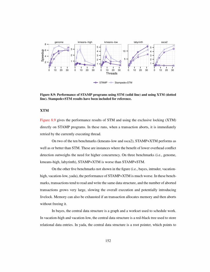
l

l

l

l

ll

ll

l

l

l

l

lll l

lll

ll

ll l l

l

l l

lll

ll

l

l l

ll

l

l

l

l

ll

l

l

l

l

lll l l lll

l

l

l

l

genome kmeans−high kmeans−low labyrinth ssca2

2

4

6

8

1

2

3

1

2

3

4

5

5

10

1

2

3

4

5

0 10 20 30 0 10 20 30 0 10 20 30 0 10 20 30 0 10 20 30

Threads

Sp

eedu

p

l STAMP Stampede+STM

Figure 8.9: Performance of STAMP programs using STM (solid line) and using XTM (dottedline). Stampede+STM results have been included for reference.

XTM

Figure 8.9 gives the performance results of STM and using the exclusive locking (XTM)

directly on STAMP programs. In these runs, when a transaction aborts, it is immediately

retried by the currently executing thread.

On two of the ten benchmarks (kmeans-low and ssca2), STAMP+XTM performs as

well as or better than STM. These are instances where the benefit of lower overhead conflict

detection outweighs the need for higher concurrency. On three benchmarks (i.e., genome,

kmeans-high, labyrinth), STAMP+XTM is worse than STAMP+STM.

On the other five benchmarks not shown in the figure (i.e., bayes, intruder, vacation-

high, vacation-low, yada), the performance of STAMP+XTM is much worse. In these bench-

marks, transactions tend to read and write the same data structure, and the number of aborted

transactions grows very large, slowing the overall execution and potentially introducing

livelock. Memory can also be exhausted if an transaction allocates memory and then aborts

without freeing it.

In bayes, the central data structure is a graph and a workset used to schedule work.

In vacation-high and vacation-low, the central data structure is a red-black tree used to store

relational data entries. In yada, the central data structure is a root pointer, which points to

152

some element of a mesh, and is used to verify the correctness of the benchmark.

As noted above, these kinds of program behaviors are unlikely to scale irrespec-

tive of transactional memory. Highly concurrent transactional memory systems can amelio-

rate the scalability problem, but solving it requires changing the program itself, and Sec-

tion 8.1.1 discusses how these centralized access patterns can be addressed by modifying

data structures.

Other Benchmarks

These scalability principles apply to other benchmarks as well. This section gives prelim-

inary results on the PARSEC suite. The PARSEC suite (Bienia et al., 2008) (v2.1) is a

collection of parallel programs that cover a number of parallelization techniques. How-

ever, none of the programs use TM, and as reported by others, most of the programs are

data-parallel (Best et al., 2011). One that is not is canneal, which simulates cache-aware

annealing to optimize routing costs.

Three variants of this program were evaluated. The first is the original PARSEC

program that uses fine-grain locking, PARSEC+FGL. The second is a manual transforma-

tion to use TinySTM instead of locks, PARSEC+STM. The third is a new program that

follows the disjoint access and virtualization principles and uses exclusive locking, New-

PARSEC+VXTM. To satisfy disjoint access, the only change made was to allocate the

main graph data structure in a NUMA-interleaved fashion to avoid congestion on physi-

cal memory controllers. Satisfying virtualization was simply a matter of converting explicit

threading to parallel loops. On Westmere with 32 threads and using the largest input size,

PARSEC+FGL is 22.3X faster than with 1 thread. On 32 threads, PARSEC+STM is 7%

faster than PARSEC+FGL, and NewPARSEC+VXTM is 16% faster. These preliminary re-

sults support the applicability of our scalability principles beyond STAMP and programs

initially written to use transactions.

153

8.2 Parallel Programming Models

The previous section described how programs can be rewritten to be more scalable by fol-

lowing the disjoint access and virtualization principles. If programs are rewritten, which

parallel programming model should they use? This section evaluates the performance of

several parallel programming models or domain-specific languages (DSLs) for graph ana-

lytics.

Graph analytics DSLs usually constrain programmers to use a subset of features

described in Section 2.2.

GraphLab (Low et al., 2010) is a shared-memory programming model for topology

or data-driven computations with autonomous or coordinated scheduling, but it is restricted

to vertex programs. A vertex program has a graph operator that can only read from and

write to the immediate neighbors of the active node. There are several priority scheduling

policies available, but the implementation of the priority scheduler is very different from

the one used in the Galois system (see Section 6.1.2).

PowerGraph (Gonzalez et al., 2012) is a distributed-memory programming model

for topology or data-driven computations with autonomous or coordinated scheduling, but

it is restricted to gather-apply-scatter (GAS) programs, which are a subset of vertex pro-

grams. Graphs are partitioned by edge where the endpoints of edges may be shared by mul-

tiple machines. Values on shared nodes can be resolved with local update and distributed

reduction. On scale-free graphs, which have many high-degree nodes, this is a useful op-

timization to improve load balancing. PowerGraph supports autonomous scheduling, but

the scheduling policy is fixed by the system and users cannot choose among autonomous

policies.

GraphChi (Kyrola et al., 2012) is a shared-memory programming model for vertex

programs that supports out-of-core processing when the input graph is too large to fit in

‡This section draws from (Nguyen et al., 2013), where the evaluation of Galois versus graph analytics DSLswas originally reported.

154

memory. GraphChi relies on a particular sorting of graph edges in order to provide I/O-

efficient access to both the in and out edges of a node. Since computation is driven by the

loading and storing of graph files, GraphChi only provides coordinated scheduling.4

Ligra (Shun and Blelloch, 2013) is a shared-memory programming model for ver-

tex programs with coordinated scheduling. A unique feature of Ligra is that it switches

between push and pull-based operators automatically based on a user-provided threshold.

Linear algebra formulations (Kepner and Gilbert, 2011) are a methodology for

exploiting the substantial expertise in parallelizing dense matrix kernels and sparse matrix-

vector multiply operations to implement graph algorithms. The basic idea is to express

graph operations as matrix operations over some algebraic semiring. For instance, in stan-

dard linear algebra, operations are over the field (R,+, ·). The shortest path can be found

by iterative application of matrix-vector multiply over the semiring (R ∪∞,min,+).

Section 2.3 shows programs can use rich programming models. However, most ex-

isting graph DSLs have restricted themselves to supporting a simple programming model,

and they do not support the more complex features such as autonomously scheduled, data-

driven computation. Next, we discuss how these simpler models can be layered on top of

the more expressive Galois system.

8.2.1 Other Domain Specific Languages in Galois

Graph analytics DSLs such GraphLab, GraphChi and Ligra can be simply layered on top

of Galois. This section describes how to implement features of the GraphLab, GraphChi,

and Ligra APIs on top of the Galois system. The Galois implementations of GraphLab

and Ligra are called GraphLab-g and Ligra-g respectively. Also, to demonstrate the ease

with which new DSLs can be implemented, a DSL called LigraChi-g is developed that

combines features of the Ligra and GraphChi systems. Figure 8.10 gives the approximate

lines of code required to implement these features on top of the Galois system.4GraphChi takes a program that could be autonomously scheduled but imposes a coordinated schedule for

execution.

155

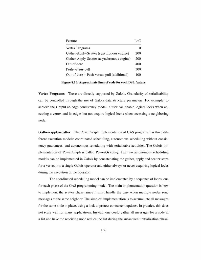
Feature LoC

Vertex Programs 0Gather-Apply-Scatter (synchronous engine) 200Gather-Apply-Scatter (asynchronous engine) 200Out-of-core 400Push-versus-pull 300Out-of-core + Push-versus-pull (additional) 100

Figure 8.10: Approximate lines of code for each DSL feature

Vertex Programs These are directly supported by Galois. Granularity of serializability

can be controlled through the use of Galois data structure parameters. For example, to

achieve the GraphLab edge consistency model, a user can enable logical locks when ac-

cessing a vertex and its edges but not acquire logical locks when accessing a neighboring

node.

Gather-apply-scatter The PowerGraph implementation of GAS programs has three dif-

ferent execution models: coordinated scheduling, autonomous scheduling without consis-

tency guarantees, and autonomous scheduling with serializable activities. The Galois im-

plementation of PowerGraph is called PowerGraph-g. The two autonomous scheduling

models can be implemented in Galois by concatenating the gather, apply and scatter steps

for a vertex into a single Galois operator and either always or never acquiring logical locks

during the execution of the operator.

The coordinated scheduling model can be implemented by a sequence of loops, one

for each phase of the GAS programming model. The main implementation question is how

to implement the scatter phase, since it must handle the case when multiple nodes send

messages to the same neighbor. The simplest implementation is to accumulate all messages

for the same node in place, using a lock to protect concurrent updates. In practice, this does

not scale well for many applications. Instead, one could gather all messages for a node in

a list and have the receiving node reduce the list during the subsequent initialization phase,

156

but this requires significant memory allocation for applications that send many messages to

the same node. The implementation used in PowerGraph-g is to have per-package message

accumulation, protected by a spin-lock. The receiver accumulates the final message value

by reading from the per-package locations.

PowerGraph supports dividing up the work of a single gather or scatter operation

for a node among different processing units, but PowerGraph-g does not yet have this opti-

mization.

Out-of-core The GraphChi implementation of out-of-core processing for vertex programs

uses a carefully designed graph file format to support I/O-efficient access to both the incom-

ing and outgoing edge values of a node. For the purpose of understanding how to provide

out-of-core processing using general reusable components, this section focuses on support-

ing only a subset of GraphChi features.

The implementation of out-of-core processing is based on incremental loading of

the compressed sparse row (CSR) format of a graph and the graph’s transpose. The trans-

pose graph represents the incoming edges of a graph and stores a copy of the edge values

of the corresponding outgoing edges. Since these values are copies, it does not support up-

dating edge values like GraphChi does; however, none of the applications described in this

chapter require updating edge values. To reduce the waiting time on I/O operations, loading

portions of the graph is double-buffered.

Push-versus-pull The push-versus-pull optimization in Ligra can be implemented as two

vertex programs that take an edge update rule and perform either a push or pull-based traver-

sal according to some threshold of active nodes to all the nodes in the graph. The Galois

implementation of Ligra is called Ligra-g. It uses the same threshold heuristic as Ligra. In

order to perform this optimization, the graph representation must store both incoming and

outgoing edges.

157

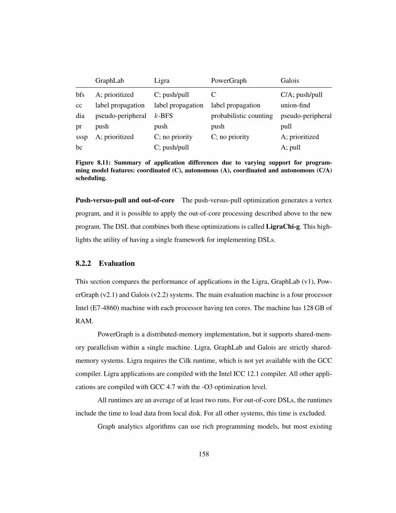
GraphLab Ligra PowerGraph Galois

bfs A; prioritized C; push/pull C C/A; push/pullcc label propagation label propagation label propagation union-finddia pseudo-peripheral k-BFS probabilistic counting pseudo-peripheralpr push push push pullsssp A; prioritized C; no priority C; no priority A; prioritizedbc C; push/pull A; pull

Figure 8.11: Summary of application differences due to varying support for program-ming model features: coordinated (C), autonomous (A), coordinated and autonomous (C/A)scheduling.

Push-versus-pull and out-of-core The push-versus-pull optimization generates a vertex

program, and it is possible to apply the out-of-core processing described above to the new

program. The DSL that combines both these optimizations is called LigraChi-g. This high-

lights the utility of having a single framework for implementing DSLs.

8.2.2 Evaluation

This section compares the performance of applications in the Ligra, GraphLab (v1), Pow-

erGraph (v2.1) and Galois (v2.2) systems. The main evaluation machine is a four processor

Intel (E7-4860) machine with each processor having ten cores. The machine has 128 GB of

RAM.

PowerGraph is a distributed-memory implementation, but it supports shared-mem-

ory parallelism within a single machine. Ligra, GraphLab and Galois are strictly shared-

memory systems. Ligra requires the Cilk runtime, which is not yet available with the GCC

compiler. Ligra applications are compiled with the Intel ICC 12.1 compiler. All other appli-

cations are compiled with GCC 4.7 with the -O3 optimization level.

All runtimes are an average of at least two runs. For out-of-core DSLs, the runtimes

include the time to load data from local disk. For all other systems, this time is excluded.

Graph analytics algorithms can use rich programming models, but most existing

158

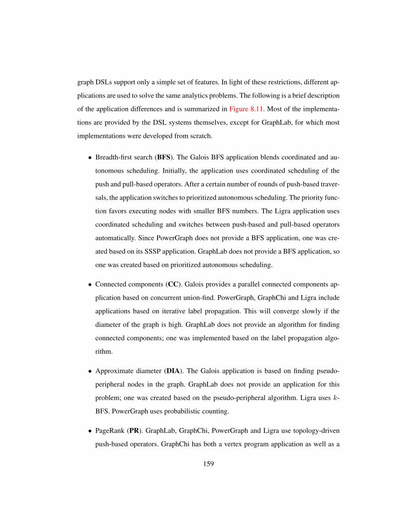
graph DSLs support only a simple set of features. In light of these restrictions, different ap-

plications are used to solve the same analytics problems. The following is a brief description

of the application differences and is summarized in Figure 8.11. Most of the implementa-

tions are provided by the DSL systems themselves, except for GraphLab, for which most

implementations were developed from scratch.

• Breadth-first search (BFS). The Galois BFS application blends coordinated and au-

tonomous scheduling. Initially, the application uses coordinated scheduling of the

push and pull-based operators. After a certain number of rounds of push-based traver-

sals, the application switches to prioritized autonomous scheduling. The priority func-

tion favors executing nodes with smaller BFS numbers. The Ligra application uses

coordinated scheduling and switches between push-based and pull-based operators

automatically. Since PowerGraph does not provide a BFS application, one was cre-

ated based on its SSSP application. GraphLab does not provide a BFS application, so

one was created based on prioritized autonomous scheduling.

• Connected components (CC). Galois provides a parallel connected components ap-

plication based on concurrent union-find. PowerGraph, GraphChi and Ligra include

applications based on iterative label propagation. This will converge slowly if the

diameter of the graph is high. GraphLab does not provide an algorithm for finding

connected components; one was implemented based on the label propagation algo-

rithm.

• Approximate diameter (DIA). The Galois application is based on finding pseudo-

peripheral nodes in the graph. GraphLab does not provide an application for this

problem; one was created based on the pseudo-peripheral algorithm. Ligra uses k-

BFS. PowerGraph uses probabilistic counting.

• PageRank (PR). GraphLab, GraphChi, PowerGraph and Ligra use topology-driven

push-based operators. GraphChi has both a vertex program application as well as a

159

|V | |E| MB Weighted MB

rmat24 17 268 1207 2281rmat27 134 2141 9637 18218twitter40 42 1469 6207 12080twitter50 51 1963 8262 16114road 24 58 422 653

Figure 8.12: Input characteristics. Number of nodes and edges is in millions. MB is the size ofCSR representation in megabytes.

gather-apply-scatter application. The latter is used because it is slightly faster. Galois

provides a pull-based PageRank application that reduces the memory overhead and

synchronization compared to push-based applications.

• Single-source shortest-paths (SSSP). The Galois SSSP application uses the data-

driven, autonomously scheduled delta-stepping algorithm, using auto-tuning to find

an optimal value of ∆ for a given input. GraphLab does not provide an SSSP applica-

tion, so one was created based on the Galois application, using the priority scheduling

available in GraphLab. PowerGraph and Ligra use Bellman-Ford, which uses coordi-

nated scheduling.

• Betweenness centrality (BC). The Galois application is based on a priority-scheduled,

pull-based algorithm for computing betweenness centrality. The priority function is

based on the BFS number of a node. The Ligra application switches between pull and

push-based operators with coordinated execution, which can have significant over-

head on large diameter graphs.

Figure 8.12 summarizes the graph inputs used. The rmat24 (a = 0.5, b = c = 0.1,

d = 0.3) and rmat27 (a = 0.57, b = c = 0.19, d = 0.05) graphs are synthetic scale-free

graphs. Following the evaluation done by Shun and Blelloch (Shun and Blelloch, 2013), the

graphs are made symmetric. The twitter40 (Kwak et al., 2010) and twitter50 (Cha et al.,

2010) graphs are real-world social network graphs. From twitter40 and twitter50, only the

160

Ligra

Galois

PowerGraph

Galois

1

10

100

1000

10000

1

10

100

1000

10000tw

itter5

0ro

ad

bfs cc dia pr sssp bfs cc dia pr sssp

Run

tim

e R

atio

s

Figure 8.13: Ratio of Ligra and PowerGraph runtimes to Galois with 40 threads. Valuesgreater than 1 (shown as blue crosses) indicate how many times faster the denominator systemis than the numerator.

largest connected component is used. Finally, road is a road network of the United States

obtained from the DIMACS shortest paths benchmark.

The road graph is naturally weighted; the weights are removed when an unweighted

graph is needed. The other four graphs are unweighted. To provide a weighted input for the

SSSP algorithms, unweighted graphs are given random edge weights in the range (0, 100].

Figure 8.13 shows the runtime ratios of the Ligra and PowerGraph applications

compared to the Galois versions on the twitter50 and road inputs for five applications. When

the Galois version runs faster, the data point is shown as a cross; otherwise it is shown as an x

(i.e., BFS on twitter50 and PR on road). The values range over several orders of magnitude.

The largest improvements are on the road graph and with respect to PowerGraph.

Figure 8.14 shows the runtime ratios of the Ligra and PowerGraph applications

compared to the Ligra-g and PowerGraph-g versions (that is, the implementations of those

DSLs in Galois). The performance of Ligra-g is roughly comparable to Ligra. PowerGraph-

g is mostly better than PowerGraph. This shows that much of the huge improvements in

Figure 8.13 come not so much from the better implementations of the DSL in Galois per

se but from the better programs that can be written when the programming model is rich

161

Ligra

Ligra−g

PowerGraph

PowerGraph−g

47 51

1

2

12

4

6

twitte

r50

road

bfs cc dia pr sssp bfs cc dia pr sssp

Run

tim

e R

atios

Figure 8.14: Ratio of Ligra and PowerGraph runtimes relative to Ligra-g and PowerGraph-g runtimes. Values greater than 1 (shown as blue crosses) indicate how many times fasterthe denominator system is than the numerator. Larger ratios shown as numbers rather thanpoints.

enough.

Comparison between the two figures can also be illuminating. For example, most

of the ratios in Figure 8.13 are greater than those in Figure 8.14, but one notable exception

is the behavior of PowerGraph with PageRank on the road graph. The Galois improvement

is about 10X while the PowerGraph-g improvement is about 50X. This suggests that the

Galois application of PageRank, which is pull-based, is not as good as the push-based algo-

rithm used by PowerGraph, on the road graph. Thus, Galois is faster than PowerGraph on

PageRank because of a more efficient implementation of a worse algorithm.

The following sections dig deeper into the performance results.

Overall results

Figure 8.15 gives the complete runtime results with 40 threads. The PageRank (PR) times

are for one iteration of the topology-driven algorithm. The betweenness centrality (BC)

times are for computing results with respect to one source node. Ligra-g and PowerGraph-g

results will be discussed in the next section.

Overall, there is a wide variation in running times across different programming

162

rmat24 rmat27 twitter40 twitter50 road

bfs Galois 0.5 1.5 0.7 2.5 0.5bfs Ligra-g 0.3 1.3 0.8 2.3 1.1bfs PowerGraph-g 10.8 84.2 28.0 37.7 17.5bfs GraphLab 12.4 83.9 26.7 60.5 4092.7bfs Ligra 0.4 1.5 1.2 2.3 2.8bfs PowerGraph 7.0 30.8 16.9 24.1 821.6

cc Galois 7.3 17.9 13.9† 39.6† 0.6cc Ligra-g 1.3 11.1 16.6 31.9 62.3cc PowerGraph-g 21.8 120.3 58.8 105.0 572.9cc GraphLab 14.1 89.6 36.0 64.5 1033.5cc Ligra 2.5 22.2 31.7 57.5 127.0cc PowerGraph 39.0 129.5 115.5 201.5 2831.5

dia Galois 1.1 5.1 2.8 5.5 2.6dia Ligra-g 2.3 21.4 19.7 44.3 8.6dia PowerGraph-g 2029.7 oom 3816.1 4841.9 2466.6dia GraphLab 84.8 478.2 192.0 257.1 21363.3dia Ligra 1.7 11.8 19.3 45.8 20.1dia PowerGraph 1239.0 oom 5376.0 7390.5 7047.5

pr Galois 1.3 10.3 6.5 10.7 0.5pr Ligra-g 1.1 15.6 4.6 11.5 0.4pr PowerGraph-g 2.1 21.0 11.7 14.0 0.2pr GraphLab 4.9 47.6 45.8 30.7 14.6pr Ligra 1.0 11.6 8.7 11.5 0.2pr PowerGraph 8.4 38.8 20.4 30.2 10.6

sssp Galois 1.9 6.0 11.6 8.6 0.6sssp Ligra-g 2.8 9.1 10.0 12.5 320.7sssp PowerGraph-g 22.8 100.0 43.3 66.8 3317.3sssp GraphLab 28.8 153.9 60.9 87.6 28.6sssp Ligra 2.3 12.3 15.9 17.8 219.4sssp PowerGraph 34.4 78.8 52.9 104.4 18919.2

bc Galois 1.3 13.7 13.0 12.0 1.3bc Ligra-g 1.4 7.6 5.3 12.9 5.1bc Ligra 1.2 5.5 6.8 13.9 6.6

Figure 8.15: Runtime in seconds of applications with 40 threads. The label oom indicates theapplication ran out of memory. In bold are the best times for each input and graph problempair. (†) indicates that the best time on CC occurred with eight threads: twitter40 (13.8 s),twitter50 (13.6 s).

163

rmat24 rmat27 twitter40 twitter50 road

Galois 17 10 14 14 8440Ligra 10 6 15 15 6262PowerGraph 9 7 8 >100

Figure 8.16: Approximate diameters computed

models solving the same problem. The variation is the least for PageRank, which is co-

ordinated and topology-driven. For the other graph problems, the performance difference

between programming models can be several orders of magnitude and is quite stark for the

road input, whose large diameter heavily penalizes coordinated scheduling of data-driven

algorithms.

The performance differences can be broadly attributed to three causes.

In some cases, a poor algorithm was selected even though a better algorithm ex-

ists and is expressible in the DSL. The PowerGraph diameter application is an example

of this. The probabilistic counting algorithm just takes too long on these inputs and gives

worse results than the Ligra algorithm, which also can be expressed as a gather-apply-

scatter program. Figure 8.16 gives the approximate diameters returned by each algorithm.

The PowerGraph algorithm quits after trying diameters up to 100. Both Galois and Ligra

algorithms give strict lower-bounds on the true diameter. The PowerGraph algorithm gives

a probabilistic estimate.

In some other cases, the same algorithm is expressed in multiple DSLs, but one

programming model just has a better system implementation. All the PageRank applications

are largely implementations of the same algorithm. Differences between implementations

are due to differences in the runtime systems for each programming model.

Finally, a DSL may be unable to capture an important algorithmic optimization—

such as when an important optimization cannot be expressed in a DSL or when it can be

expressed but the implementation of the DSL cannot adequately exploit it.

An example of not being able to express an optimization is the lack of priority

164

rmat24 rmat27 twitter40 twitter50 road

8x16 64x16 8x16 64x16 8x16 64x16 8x16 64x16 8x16 64x16

bfs 29.2 21.8 73.0 28.6 73.2 38.5 81.5 50.8 161.5 821.6cc 114.5 53.5 270.5 71.5 270.0 90.0 406.0 112.0pr 11.6 9.9 43.2 14.8 30.5 17.6 42.3 16.4 4.1 5.8sssp 112.0 76.9 173.9 63.0 175.2 111.0 321.9 127.5

Figure 8.17: Runtime in seconds of PowerGraph applications on a distributed system witheight or 64 machines

scheduling for the Ligra and PowerGraph applications for SSSP. GraphLab supports priority

scheduling, so although the GraphLab SSSP application is worse on scale-free inputs, it

performs much better than Ligra and PowerGraph on the road input due to its support for

priority scheduling. Thus, in some cases, it is preferable to have inefficient support for

priority scheduling than no support at all.

Another example is the push-versus-pull optimization implemented in Ligra. In

principle, this optimization can be implemented in any DSL that supports coordinated

scheduling of vertex programs, like GraphLab, but GraphLab does not provide any sup-

port for user-visible concurrent bag or worklist objects, so it is not possible to efficiently

switch between push and pull traversals.

An example of the inability to exploit an optimization is the GraphLab diameter

application. The faster pseudo-peripheral algorithm was implemented in GraphLab, but be-

cause of large overheads in starting and stopping parallel execution, which are required for

the sequential composition of the parallel breadth-first searches, the overall application has

very poor performance.

Figure 8.17 shows the performance of PowerGraph when run on a distributed sys-

tem, the Stampede cluster at the Texas Advanced Computing Center (TACC). Each machine

used is an instance of a two processor Intel (E5-2680) machine with each processor having

eight cores. Each machine has 32 GB of RAM. Given the poor performance of the con-

165

rmat24 rmat27 twitter40 twitter50 road

bfs Galois 1.4 4.3 2.2 4.8 0.8bfs Ligra-g 1.0 4.5 2.8 5.4 1.0bfs PowerGraph-g 7.2 47.2 22.7 37.7 5.8bfs GraphLab 20.3 90.2 52.3 60.6 3177.2bfs Ligra 0.6 2.1 1.8 2.9 2.1bfs PowerGraph 11.9 58.7 29.4 42.8 452.8

cc Galois 1.7 12.9 13.8† 13.6† 1.0cc Ligra-g 4.3 33.5 35.8 61.9 236.8cc PowerGraph-g 46.4 194.8 144.2 320.1 1336.3cc GraphLab 36.1 130.7 89.3 91.5 1512.6cc Ligra 2.7 24.9 27.1 49.4 141.0cc PowerGraph 70.0 280.5 226.5 384.0 2846.5

dia Galois 3.5 13.5 7.4 9.8 3.7dia Ligra-g 8.8 55.8 54.1 89.4 21.7dia PowerGraph-g 2678.4 oom 3969.8 6094.5 3151.5dia GraphLab 177.5 810.0 259.6 230.8 20047.4dia Ligra 5.1 35.6 39.1 68.0 37.2dia PowerGraph 3528.0 oom 14877.0 20161.0 9617.5

pr Galois 2.2 15.6 8.1 13.1 1.0pr Ligra-g 2.7 25.0 12.2 22.9 0.9pr PowerGraph-g 2.1 24.5 10.5 13.0 0.7pr GraphLab 13.3 92.5 30.8 30.2 28.2pr Ligra 2.9 34.7 20.6 34.0 0.4pr PowerGraph 12.8 67.2 37.0 51.0 16.6

sssp Galois 3.4 15.4 12.2 14.8 1.1sssp Ligra-g 7.2 25.2 17.9 24.7 1154.2sssp PowerGraph-g 38.8 114.6 68.0 140.8 9071.7sssp GraphLab 84.0 548.1 199.9 276.2 60.1sssp Ligra 4.7 22.0 17.7 29.9 440.8sssp PowerGraph 54.2 141.4 90.7 189.1 23556.2

bc Galois 4.3 27.0 21.2 18.9 1.9bc Ligra-g 4.0 20.6 17.7 30.7 3.6bc Ligra 2.2 11.3 11.2 17.8 5.4

Figure 8.18: Runtime in seconds of applications with 8 threads. The label oom indicates theapplication ran out of memory. In bold are the best times for each input and graph problempair; in all but two cases, best times are with 40 threads (see Figure 8.15).

166

nected components and SSSP PowerGraph implementations on the road graph on shared-

memory machines, they were not run on the distributed machine. Even with 64 machines

(64 · 16 = 1024 cores), the performance is worse than that of the best implementation on

a single machine with 8 cores and 4 times the RAM for all but one application-input com-

bination (see Figure 8.17 and Figure 8.18). The one slower combination is PageRank on

rmat27 where Galois takes 15.6 seconds and PowerGraph takes 14.8 seconds.

Comparison of Implementations

Figure 8.15 also shows the performance results of Ligra and PowerGraph compared to

the implementations of their programming models with the Galois system, Ligra-g and

PowerGraph-g respectively.

Overall, the Galois implementations of graph DSLs do better than the original DSL

implementations, although this varies from DSL to DSL. If pairs of Ligra and Ligra-g run-

times are considered for each graph problem, input and number of threads, in 18/30 ≈ 60%

of the pairs, the Galois version is faster. However, due to compiler incompatibilities, a differ-

ent compiler was used for each version of the application. Considering pairs of PowerGraph

and PowerGraph-g, runtimes, 18/24 = 75% of the pairs favor the Galois version. As noted

earlier, PowerGraph supports distributed-memory execution as well, so some portion of the

performance gap is due to the additional overhead of supporting distributed-memory exe-

cution and not using it. For GraphLab and Galois, all of the pairs favor Galois, although in

this case, the Galois applications include optimizations that could not be implemented in

GraphLab, like push-versus-pull.

Some improvements can be made to the Galois versions of these DSLs. For in-

stance, the Ligra version of the diameter application tends to be faster than the Ligra-g

version, and the PowerGraph version of BFS tends to scale better than the PowerGraph-g

version, but overall, the results suggest that the Galois infrastructure is a reasonable sub-

strate on which graph DSLs can be built.

167

rmat24 rmat27 twitter40 twitter50 road

bfs LigraChi-g 9 133 187 960 12cc LigraChi-g 17 205 175 310 169cc GraphChi 223 1164 870 1179 120dia LigraChi-g 21 192 265 697 29pr LigraChi-g 16 143 90 114 6pr GraphChi 38 308 154 220 13sssp LigraChi-g 36 1127 3227 4873 790bc LigraChi-g 18 237 251 1561 14

Figure 8.19: Runtime in seconds of applications on small memory machine with eight threads

Evaluation of Out-of-core DSLs

To evaluate the out-of-core DSLs, GraphChi and LigraChi-g (the combination of Ligra and

GraphChi in Galois), a machine with less memory is used. Instead of the machine with

128 GB RAM used in the previous figures, this machine has 24 GB of RAM. It is a two

processor Intel (X5570) machine. Each processor has four cores. To test the out-of-core

capability, each DSL is given a memory budget of 2 GB of RAM to store graph data. This

includes graph adjacency information and edge values, but it does not include user data

allocated for a node nor any additional user or runtime-allocated structures. The entire road

graph fits in this memory budget.

Figure 8.19 gives the performance of the out-of-core DSLs. Inputs were stored on a

7200 RPM SATA drive. GraphChi allows separate configuration of load threads, which read

the graph file, and execute threads, which run the vertex program. For these experiments,

the number of threads refers to the number of execute threads. Two load threads are always

used.

These out-of-core experiments highlight the impact of having enough memory for

graph analytics applications. Ignoring differences in processors but keeping the number of

threads the same, on the larger inputs, i.e., rmat27, twitter40 and twitter50, running in a

memory-constrained environment with LigraChi-g (see Figure 8.19) is between 3.4X and

168

197X slower than performing the same algorithm with Ligra-g on machine m4x10 (compare

with Figure 8.18), an unconstrained memory environment.

These results provide more context for the claim by Kyrola et al. that out-of-core

execution of graph analytics only incurs a modest performance penalty (Kyrola et al., 2012).

The slowdown is between 3.4X and 7.8X for the connected components, approx-

imate diameter and PageRank applications. Considering a 5X reduction in memory, these

results suggest a reasonable trade-off between space and time for connected components

and PageRank. For the approximate diameter application, there are additional gains from

switching to the more expressive Galois programming model.

For the other applications, the slowdown ranges between 11.5X and 197X, not in-

cluding the additional slowdown of Ligra or Ligra-g versus Galois. The out-of-core DSLs

impose a particular scheduling of activities that optimizes I/O operations, but that order may

not be efficient from the application standpoint. For more effective out-of-core implemen-

tations of these applications, more attention should be paid towards the joint optimization

of application and I/O-level scheduling.

8.3 Related Work

There have been several performance evaluations of hardware transactional memory (Dice

et al., 2009; Dalessandro et al., 2011; Wang et al., 2012a; Yoo et al., 2013; Diegues et al.,

2014), and as noted in Section 8.1.3, some part of the evaluation in this dissertation repro-

duces the results of Wang et al. Intel has also released HTM support in their fourth genera-

tion Intel Core i7 (Haswell) processors, but it has since been disabled due to reports of an

implementation bug (Intel, 2014). Prior to its disabling, there were several evaluations of

the Haswell HTM (Yoo et al., 2013; Diegues et al., 2014). The hardware is targeted towards

short-running, fine-grain transaction programs, which are not the kinds of transactions that

arise in STAMP programs. The results of Yoo et al. on STAMP programs using four threads

show abort rates significantly higher than using an STM, which suggests a large number of

169

capacity or false conflicts even at low levels of parallelism. The highest speedup over se-

quential reported by Diegues et al. for HTM is 3.5X on 8 threads for kmeans. In any event,

the goal of this dissertation is not strictly to evaluate HTM implementations but to show

how simple mechanisms are sufficient to efficiently execute programs with transactional

semantics.

SwissTM (Dragojevic et al., 2009) has been shown to perform slightly better than

TinySTM, which was used as a representative STM in Section 8.1, but the STAMP bench-

marks where SwissTM outperforms TinySTM the most (by 1.2X–1.5X)—intruder, kmeans-

high, yada—also have poor scalability, so the actual performance difference is small.

There are several proposals for parallel programming models that support transac-

tional behavior (Adl-Tabatabai et al., 2006; Carlstrom et al., 2006; Chamberlain et al., 2007;

Ni et al., 2008), but in these cited works, transactions are fine-grain, and no separation is

made between schedulers and user data structures, which is crucial to simplifying transac-

tion implementation. Automatic Mutual Exclusion (AME) (Abadi et al., 2011) introduced a

higher level abstraction for transactional execution where code blocks are transactional by

default. This matches the spirit of loop-based transactions described here, but the work on

AME is mainly concerned with semantics rather than performance.

170

Chapter 9

Conclusion

The growth of data center and mobile computing has renewed interest in computing effi-

ciency and performance. Prior work on parallelism assumed that activities are independent

or that dependences are subsumed by fork-join control dependences, so current general-

purpose runtime schedulers embody only a few simple scheduling policies. In contrast,

handwritten schedulers for parallel implementations of irregular algorithms often use care-

fully crafted policies that trade-off excess work for increased parallelism, but they increase

the burden of parallel programming and may be difficult to reuse for other algorithms. Ad-

ditionally, prior programming models often did not clearly distinguish the computational

operator from its scheduling and from its data structures.

This dissertation described the design and implementation of a new parallel pro-

gramming system, Galois, that surmounts these challenges and argues that a distinction

between computational operators from scheduling and from data structures is necessary for

high performance, high productivity programming models. To support this point, it showed

that the performance of a well-studied benchmark suite can be significantly improved by

factoring programs along these lines. To show that these benefits can be achieved without

much programmer effort, the Galois system was evaluated against existing programming

models for graph analytics, and the results showed orders of magnitude performance im-

171

provements. The benefit is mainly due to better support for more efficient algorithms, but if

a simpler programming model is desired, it can be layered on top of the Galois system. The

Galois system also facilitates efficient deterministic scheduling.

Overall, these results suggest a promising new direction for the design of program-

ming models—one that sees a parallel program as operator + schedule + parallel data struc-

ture.

172

Bibliography

M. Abadi, A. Birrell, T. Harris, and M. Isard. Semantics of transactional memory and au-

tomatic mutual exclusion. ACM Transactions on Programming Languages and Systems,

33(1):2:1–2:50, Jan. 2011. ISSN 0164-0925. doi: 10.1145/1889997.1889999.

A.-R. Adl-Tabatabai, B. T. Lewis, V. Menon, B. R. Murphy, B. Saha, and T. Shpeisman.

Compiler and runtime support for efficient software transactional memory. In Proceed-

ings of the ACM SIGPLAN Conference on Programming Language Design and Imple-

mentation, PLDI, pages 26–37, New York, NY, USA, 2006. ACM. ISBN 1-59593-320-4.

doi: 10.1145/1133981.1133985.

A. Agarwal, O. Chapelle, M. Dudık, and J. Langford. A reliable effective terascale linear

learning system. Journal of Machine Learning Research, 15(1):1111–1133, Jan. 2014.

ISSN 1532-4435. URL http://jmlr.org/papers/v15/agarwal14a.html.

E. Allen, D. Chase, J. Hallett, V. Luchangco, J.-W. Maessen, S. Ryu, G. L. Steele Jr., and

S. Tobin-Hochstadt. The Fortress language specification version 1.0. Technical report,

Sun Microsystems, 2007.

F. E. Allen. Control flow analysis. SIGPLAN Notices, 5(7):1–19, July 1970. ISSN 0362-

1340. doi: 10.1145/390013.808479.

F. E. Allen and J. Cocke. A program data flow analysis procedure. Communications of the

ACM, 19(3):137–147, 1976. ISSN 0001-0782. doi: 10.1145/360018.360025.

173

N. Amenta, S. Choi, and G. Rote. Incremental constructions con brio. In Proceedings of

the Symposium on Computational Geometry, SCG, pages 211–219, New York, NY, USA,

2003. ACM. ISBN 1-58113-663-3. doi: 10.1145/777792.777824.

L. O. Andersen. Program Analysis and Specialization for the C Programming Language.

PhD thesis, DIKU, University of Copenhagen, May 1994. (DIKU report 94/19).

A. Aviram, S.-C. Weng, S. Hu, and B. Ford. Efficient system-enforced determinis-

tic parallelism. In Proceedings of the USENIX Conference on Operating Systems

Design and Implementation, OSDI, Berkeley, CA, USA, 2010. USENIX Associa-

tion. URL https://www.usenix.org/conference/osdi10/efficient-

system-enforced-deterministic-parallelism.

H. Avni and N. Shavit. Maintaining consistent transactional states without a global clock. In

Proceedings of the International Colloquium on Structural Information and Communica-

tion Complexity, SIROCCO, pages 131–140, Berlin, Heidelberg, 2008. Springer-Verlag.

ISBN 978-3-540-69326-0. doi: 10.1007/978-3-540-69355-0_12.

D. A. Bader and V. Sachdeva. A cache-aware parallel implementation of the push-relabel

network flow algorithm and experimental evaluation of the gap relabeling heuristic. In

Proceedings of the International Conference on Parallel and Distributed Computing Sys-

tems, PDCS, Sep. 2005.

M. M. Baskaran, N. Vydyanathan, U. K. R. Bondhugula, J. Ramanujam, A. Roun-

tev, and P. Sadayappan. Compiler-assisted dynamic scheduling for effective paral-

lelization of loop nests on multicore processors. In Proceedings of the 14th ACM

SIGPLAN Symposium on Principles and Practice of Parallel Programming, PPoPP

’09, pages 219–228, New York, NY, USA, 2009. ACM. ISBN 978-1-60558-397-6.

doi: 10.1145/1504176.1504209. URL http://doi.acm.org/10.1145/

1504176.1504209.

174

M. Bauer, S. Treichler, E. Slaughter, and A. Aiken. Legion: Expressing locality and inde-

pendence with logical regions. In Proceedings of the International Conference on High

Performance Computing, Networking, Storage and Analysis, SC, pages 66:1–66:11, Los

Alamitos, CA, USA, 2012. IEEE Computer Society Press. ISBN 978-1-4673-0805-2.

doi: 10.1109/SC.2012.71.

S. Beamer, K. Asanovic, and D. Patterson. Direction-optimizing breadth-first search. In

Proceedings of the International Conference on High Performance Computing, Network-

ing, Storage and Analysis, SC, pages 12:1–12:10, Los Alamitos, CA, USA, 2012. IEEE

Computer Society Press. ISBN 978-1-4673-0805-2. doi: 10.1109/SC.2012.50.

R. Bellman. On a routing problem. Quarterly of Applied Mathematics, 16(1):87–90, 1958.

H. Berenson, P. Bernstein, J. Gray, J. Melton, E. O’Neil, and P. O’Neil. A critique of ANSI

SQL isolation levels. In Proceedings the ACM SIGMOD International Conference on

Management of Data, SIGMOD, pages 1–10, New York, NY, USA, 1995. ACM. ISBN

0-89791-731-6. doi: 10.1145/223784.223785.

T. Bergan, O. Anderson, J. Devietti, L. Ceze, and D. Grossman. CoreDet: a compiler and

runtime system for deterministic multithreaded execution. In Proceedings of the Inter-

national Conference on Architectural Support for Programming Languages and Operat-

ing Systems, ASPLOS, pages 53–64, New York, NY, USA, 2010a. ACM. ISBN 978-1-

60558-839-1. doi: 10.1145/1736020.1736029.

T. Bergan, N. Hunt, L. Ceze, and S. D. Gribble. Deterministic process groups

in dOS. In Proceedings of the USENIX Conference on Operating Systems De-

sign and Implementation, OSDI, Berkeley, CA, USA, 2010b. USENIX Association.

URL https://www.usenix.org/conference/osdi10/deterministic-

process-groups-dos.

E. D. Berger, K. S. McKinley, R. D. Blumofe, and P. R. Wilson. Hoard: a scalable memory

175

allocator for multithreaded applications. SIGPLAN Notices, 35(11):117–128, Nov. 2000.

ISSN 0362-1340. doi: 10.1145/356989.357000.

E. D. Berger, T. Yang, T. Liu, and G. Novark. Grace: safe multithreaded programming for

C/C++. In Proceedings of the ACM SIGPLAN Conference on Object-oriented Program-

ming Systems, Languages, and Applications, OOPSLA, pages 81–96, New York, NY,

USA, 2009. ACM. ISBN 978-1-60558-766-0. doi: 10.1145/1640089.1640096.

D. P. Bertsekas and J. N. Tsitsiklis. Parallel and distributed computation: numerical meth-

ods. Prentice-Hall, Inc., Upper Saddle River, NJ, USA, 1989. ISBN 0-13-648700-9.

D. P. Bertsekas, F. Guerriero, and R. Musmanno. Parallel asynchronous label-correcting

methods for shortest paths. Journal of Optimization Theory and Applications, 88(2):

297–320, Feb. 1996. ISSN 0022-3239. doi: 10.1007/BF02192173.

M. J. Best, S. Mottishaw, C. Mustard, M. Roth, A. Fedorova, and A. Brownsword. Synchro-

nization via scheduling: Techniques for efficiently managing shared state. In Proceedings

of the ACM SIGPLAN Conference on Programming Language Design and Implementa-

tion, PLDI, pages 640–652, New York, NY, USA, 2011. ACM. ISBN 978-1-4503-0663-

8. doi: 10.1145/1993498.1993573.

C. Bienia, S. Kumar, J. P. Singh, and K. Li. The PARSEC benchmark suite: Characteriza-

tion and architectural implications. In Proceedings of the International Conference on

Parallel Architectures and Compilation Techniques, PACT, pages 72–81, New York, NY,

USA, 2008. ACM. ISBN 978-1-60558-282-5. doi: 10.1145/1454115.1454128.

G. E. Blelloch. Nesl: A nested data-parallel language. Technical report, Carnegie Mellon

University, Pittsburgh, PA, USA, 1992.

G. E. Blelloch, J. T. Fineman, P. B. Gibbons, and J. Shun. Internally deterministic parallel

algorithms can be fast. In Proceedings of the ACM SIGPLAN symposium on Principles

176

and Practice of Parallel Programming, PPoPP, pages 181–192, New York, NY, USA,

2012. ACM. ISBN 978-1-4503-1160-1. doi: 10.1145/2145816.2145840.

R. D. Blumofe, C. F. Joerg, B. C. Kuszmaul, C. E. Leiserson, K. H. Randall, and Y. Zhou.

Cilk: An efficient multithreaded runtime system. In Proceedings of the SIGPLAN Sympo-

sium on Principles and Practice of Parallel Programming, PPoPP, pages 207–216, New

York, NY, USA, 1995. ACM. ISBN 0-89791-700-6. doi: 10.1145/209936.209958.

R. L. Bocchino, V. S. Adve, and B. L. Chamberlain. Software transactional memory for

large scale clusters. In Proceedings of the ACM SIGPLAN Symposium on Principles and

Practice of Parallel Programming, PPoPP, pages 247–258, New York, NY, USA, 2008.

ACM. ISBN 978-1-59593-795-7. doi: 10.1145/1345206.1345242.

R. L. Bocchino, Jr., V. S. Adve, S. V. Adve, and M. Snir. Parallel programming

must be deterministic by default. In Proceedings of the USENIX Conference on

Hot Topics in Parallelism, HotPar, Berkeley, CA, USA, 2009. USENIX Associa-

tion. URL https://www.usenix.org/legacy/events/hotpar09/tech/

full_papers/bocchino/bocchino.pdf.

R. L. Bocchino, Jr., S. Heumann, N. Honarmand, S. V. Adve, V. S. Adve, A. Welc, and

T. Shpeisman. Safe nondeterminism in a deterministic-by-default parallel language. In

Proceedings of the ACM SIGPLAN-SIGACT Symposium on Principles of Programming

Languages, POPL, pages 535–548, New York, NY, USA, 2011. ACM. ISBN 978-1-

4503-0490-0. doi: 10.1145/1926385.1926447.

G. Bosilca, A. Bouteiller, A. Danalis, T. Herault, P. Lemarinier, and J. Dongarra. DAGuE: A

generic distributed DAG engine for high performance computing. Parallel Computing, 38

(1-2):37–51, Jan. 2012. ISSN 0167-8191. doi: 10.1016/j.parco.2011.10.003.

A. Bowyer. Computing Dirichlet tessellations. The Computer Journal, 24(2):162–166,

1981. doi: 10.1093/comjnl/24.2.162.

177

U. Brandes. A faster algorithm for betweenness centrality. Journal of Mathematical Soci-

ology, 25(2):163–177, 2001. doi: 10.1080/0022250X.2001.9990249.

S. Brin and L. Page. The anatomy of a large-scale hypertextual web search engine.

Computer Networks and ISDN Systems, 30(17):107 – 117, 1998. ISSN 0169-7552.

doi: 10.1016/S0169-7552(98)00110-X. Proceedings of the Seventh Interna-

tional World Wide Web Conference.

N. G. Bronson, J. Casper, H. Chafi, and K. Olukotun. A practical concurrent binary search

tree. In Proceedings of the ACM SIGPLAN Symposium on Principles and Practice of

Parallel Programming, PPoPP, pages 257–268, New York, NY, USA, 2010. ACM. ISBN

978-1-60558-877-3. doi: 10.1145/1693453.1693488.

S. Burckhardt, A. Baldassin, and D. Leijen. Concurrent programming with revisions and

isolation types. In Proceedings of the ACM International Conference on Object-oriented

Programming, Systems, Languages, and Applications, OOPSLA, pages 691–707, New

York, NY, USA, 2010. ACM. ISBN 978-1-4503-0203-6. doi: 10.1145/1869459.

1869515.

C. Cao Minh, J. Chung, C. Kozyrakis, and K. Olukotun. STAMP: Stanford transactional

applications for multi-processing. In Proceedings of the IEEE International Symposium

on Workload Characterization, IISWC, pages 35–46, 2008. doi: 10.1109/IISWC.

2008.4636089.

B. D. Carlstrom, A. McDonald, H. Chafi, J. Chung, C. C. Minh, C. Kozyrakis, and

K. Olukotun. The Atomos transactional programming language. In Proceedings of

the ACM SIGPLAN Conference on Programming Language Design and Implementa-

tion, PLDI, pages 1–13, New York, NY, USA, 2006. ACM. ISBN 1-59593-320-4.

doi: 10.1145/1133981.1133983.

M. Cha, H. Haddadi, F. Benevenuto, and K. P. Gummadi. Measuring user influence

178

in Twitter: the million follower fallacy. In Proceedings of the International AAAI

Conference on Weblogs and Social Media, ICWSM, Menlo Park, CA, USA, 2010.

The AAAI Press. URL http://www.aaai.org/ocs/index.php/ICWSM/

ICWSM10/paper/view/1538.

B. Chamberlain, D. Callahan, and H. Zima. Parallel programmability and the chapel lan-

guage. International Journal of High Performance Computing Applications, 21(3):291–

312, Aug. 2007. ISSN 1094-3420. doi: 10.1177/1094342007078442.

K. M. Chandy and J. Misra. The drinking philosophers problem. ACM Transactions

on Programming Languages and Systems, 6(4):632–646, Oct. 1984. ISSN 0164-0925.

doi: 10.1145/1780.1804.

P. Charles, C. Grothoff, V. Saraswat, C. Donawa, A. Kielstra, K. Ebcioglu, C. von Praun,

and V. Sarkar. X10: An object-oriented approach to non-uniform cluster computing. In

Proceedings of the ACM SIGPLAN Conference on Object-oriented Programming, Sys-

tems, Languages, and Applications, OOPSLA, pages 519–538, New York, NY, USA,

2005. ACM. ISBN 1-59593-031-0. doi: 10.1145/1094811.1094852.

D. Chazan and W. Miranker. Chaotic relaxation. Linear Algebra and its Applications, 2(2):

199–222, 1969. ISSN 0024-3795. doi: 10.1016/0024-3795(69)90028-7.

B. Chazelle. The soft heap: an approximate priority queue with optimal error rate. Journal

of the ACM, 47(6):1012–1027, Nov. 2000. ISSN 0004-5411. doi: 10.1145/355541.

355554.

B. V. Cherkassy and A. V. Goldberg. On implementing push-relabel method for the max-

imum flow problem. In Proceedings of the International Conference on Integer Pro-

gramming and Combinatorial Optimization, IPCO, pages 157–171, London, UK, 1995.

Springer-Verlag. ISBN 3-540-59408-6. doi: 10.1145/645586.659457.

179

L. P. Chew. Guaranteed-quality mesh generation for curved surfaces. In Proceedings of the

Symposium on Computational Geometry, SCG, pages 274–280, New York, NY, USA,

1993. ACM. ISBN 0-89791-582-8. doi: 10.1145/160985.161150.

K. L. Clarkson and P. W. Shor. Applications of random sampling in computational ge-

ometry, II. Discrete and Computational Geometry, 4(1):387–421, 1989. ISSN 0179-

5376. doi: 10.1007/BF02187740. URL http://dx.doi.org/10.1007/

BF02187740.

A. T. Clements, M. F. Kaashoek, and N. Zeldovich. Scalable address spaces using RCU

balanced trees. In Proceedings of the International Conference on Architectural Support

for Programming Languages and Operating Systems, ASPLOS, pages 199–210, New

York, NY, USA, 2012. ACM. ISBN 978-1-4503-0759-8. doi: 10.1145/2150976.

2150998.

A. T. Clements, M. F. Kaashoek, N. Zeldovich, R. T. Morris, and E. Kohler. The scalable

commutativity rule: Designing scalable software for multicore processors. In Proceed-

ings of the ACM Symposium on Operating Systems Principles, SOSP, pages 1–17, New

York, NY, USA, 2013. ACM. ISBN 978-1-4503-2388-8. doi: 10.1145/2517349.

2522712.

T. Cormen, C. Leiserson, R. Rivest, and C. Stein, editors. Introduction to Algorithms. MIT

Press, 2009. ISBN 978-0262033848.

H. Cui, J. Simsa, Y.-H. Lin, H. Li, B. Blum, X. Xu, J. Yang, G. A. Gibson, and R. E. Bryant.

Parrot: A practical runtime for deterministic, stable, and reliable threads. In Proceedings

of the ACM Symposium on Operating Systems Principles, SOSP, pages 388–405, New

York, NY, USA, 2013. ACM. ISBN 978-1-4503-2388-8. doi: 10.1145/2517349.

2522735.

L. Dagum and R. Menon. OpenMP: An industry-standard API for shared-memory pro-

180

gramming. IEEE Computational Science and Engineering, 5(1):46–55, 1998. doi: 10.

1109/99.660313.

L. Dalessandro, F. Carouge, S. White, Y. Lev, M. Moir, M. L. Scott, and M. F. Spear. Hybrid

NOrec: a case study in the effectiveness of best effort hardware transactional memory. In

Proceedings of the International Conference on Architectural Support for Programming

Languages and Operating Systems, ASPLOS, pages 39–52, 2011. ISBN 978-1-4503-

0266-1. doi: 10.1145/1950365.1950373.

R. Das, J. Wu, J. Saltz, H. Berryman, and S. Hiranandani. Distributed memory compiler

design for sparse problems. IEEE Transactions on Computers, 44(6):737–753, 1995.

ISSN 0018-9340. doi: 10.1109/12.391186.

J. Dean and S. Ghemawat. MapReduce: Simplified data processing on large clus-

ters. In Proceedings of the USENIX Conference on Operating Systems De-

sign and Implementation, OSDI, Berkeley, CA, USA, 2004. USENIX Associa-

tion. URL http://usenix.org/publications/library/proceedings/

osdi04/tech/full_papers/dean/dean.pdf.

J. Devietti, J. Nelson, T. Bergan, L. Ceze, and D. Grossman. RCDC: a relaxed consis-

tency deterministic computer. In Proceedings of the International Conference on Archi-

tectural Support for Programming Languages and Operating Systems, ASPLOS, pages

67–78, New York, NY, USA, 2011. ACM. ISBN 978-1-4503-0266-1. doi: 10.1145/

1950365.1950376.

D. Dice, O. Shalev, and N. Shavit. Transactional locking II. In Proceedings of the In-

ternational Conference on Distributed Computing, DISC, pages 194–208, Berlin, Hei-

delberg, 2006. Springer-Verlag. ISBN 3-540-44624-9, 978-3-540-44624-8. doi: 10.

1007/11864219_14.

D. Dice, Y. Lev, M. Moir, and D. Nussbaum. Early experience with a commercial hard-

181

ware transactional memory implementation. In Proceedings of the International Con-

ference on Architectural Support for Programming Languages and Operating Systems,

ASPLOS, pages 157–168, 2009. ISBN 978-1-60558-406-5. doi: 10.1145/1508244.

1508263.

N. Diegues, P. Romano, and L. Rodrigues. Virtues and limitations of commodity hardware

transactional memory. In Proceedings of the International Conference on Parallel Archi-

tectures and Compilation, PACT, pages 3–14, New York, NY, USA, 2014. ACM. ISBN

978-1-4503-2809-8. doi: 10.1145/2628071.2628080.

E. W. Dijkstra. A note on two problems in connexion with graphs. Numerische Mathematik,

1(1):269–271, 1959.

S. Dolev, D. Hendler, and A. Suissa. CAR-STM: Scheduling-based collision avoidance and

resolution for software transactional memory. In Proceedings of the ACM Symposium

on Principles of Distributed Computing, PODC, pages 125–134, New York, NY, USA,

2008. ACM. ISBN 978-1-59593-989-0. doi: 10.1145/1400751.1400769.

A. Dragojevic, R. Guerraoui, and M. Kapalka. Stretching transactional memory. In Pro-

ceedings of the ACM SIGPLAN Conference on Programming Language Design and Im-

plementation, PLDI, pages 155–165, New York, NY, USA, 2009. ACM. ISBN 978-1-

60558-392-1. doi: 10.1145/1542476.1542494.

A. Drebes, K. Heydemann, N. Drach, A. Pop, and A. Cohen. Topology-aware and

dependence-aware scheduling and memory allocation for task-parallel languages. ACM

Transactions on Architecture and Code Optimization, 11(3):30:1–30:25, Aug. 2014.

ISSN 1544-3566. doi: 10.1145/2641764.

A. Duran, J. Corbalan, and E. Ayguade. Evaluation of OpenMP task scheduling strategies.

In Proceedings of the Conference on OpenMP in a new era of parallelism, IWOMP,

182

pages 100–110, Berlin, Heidelberg, 2008. Springer-Verlag. doi: 10.1007/978-3-

540-79561-2_9.

R.-E. Fan, K.-W. Chang, C.-J. Hsieh, X.-R. Wang, and C.-J. Lin. LIBLINEAR: A library

for large linear classification. Journal of Machine Learning Research, 9:1871–1874, June

2008. ISSN 1532-4435. URL http://jmlr.org/papers/v9/fan08a.html.

P. Feautrier and C. Lengauer. The Polyhedron Model. In D. Padua, editor, Encyclopedia of

Parallel Programming. Springer, 2011. ISBN 978-0-387-09765-7.

P. Felber, C. Fetzer, and T. Riegel. Dynamic performance tuning of word-based software

transactional memory. In Proceedings of the ACM SIGPLAN Symposium on Princi-

ples and Practice of Parallel Programming, PPoPP, pages 237–246, 2008. ISBN 978-1-

59593-795-7. doi: 10.1145/1345206.1345241.

P. Flajolet and G. N. Martin. Probabilistic counting algorithms for data base applications.

Journal of Computer and System Sciences, 31(2):182–209, Sep. 1985. ISSN 0022-0000.

doi: 10.1016/0022-0000(85)90041-8.

L. R. Ford and D. R. Fulkerson. Flows in Networks. Princeton University Press, 1962.

J. Friedman, T. Hastie, and R. Tibshirani. Regularization paths for generalized linear models

via coordinate descent. Journal of Statistical Software, 33(1):1–22, 2010.

S. Ghemawat and P. Menage. TCMalloc: Thread-caching malloc. http://goog-

perftools.sourceforge.net/doc/tcmalloc.html, 2014.

J. R. Gilbert and R. Schreiber. Highly parallel sparse cholesky factorization. SIAM Jour-

nal on Scientific and Statistical Computing, 13(5):1151–1172, 1992. ISSN 0196-5204.

doi: 10.1137/0913067.

A. V. Goldberg and R. E. Tarjan. A new approach to the maximum-flow problem. Journal

of the ACM, 35(4):921–940, 1988. ISSN 0004-5411. doi: 10.1145/48014.61051.

183

J. E. Gonzalez, Y. Low, H. Gu, D. Bickson, and C. Guestrin. PowerGraph: distributed

graph-parallel computation on natural graphs. In Proceedings of the USENIX Confer-

ence on Operating Systems Design and Implementation, OSDI, pages 17–30, Hollywood,

CA, 2012. USENIX. ISBN 978-1-931971-96-6. URL https://www.usenix.org/

conference/osdi12/technical-sessions/presentation/gonzalez.

Y. Guo, J. Zhao, V. Cave, and V. Sarkar. SLAW: A scalable locality-aware adaptive work-

stealing scheduler for multi-core systems. In Proceedings of the ACM SIGPLAN Sympo-

sium on Principles and Practice of Parallel Programming, PPoPP, pages 341–342, New

York, NY, USA, 2010. ACM. ISBN 978-1-60558-877-3. doi: 10.1145/1693453.

1693504.

R. H. Halstead, Jr. MULTILISP: A language for concurrent symbolic computation. ACM

Transactions on Programming Languages and Systems, 7(4):501–538, 1985. ISSN 0164-

0925. doi: 10.1145/4472.4478.

B. Hardekopf and C. Lin. The ant and the grasshopper: Fast and accurate pointer analysis

for millions of lines of code. In Proceedings of the ACM SIGPLAN Conference on Pro-

gramming Language Design and Implementation, PLDI, pages 290–299, New York, NY,

USA, 2007. ACM. ISBN 978-1-59593-633-2. doi: 10.1145/1250734.1250767.

T. Harris and K. Fraser. Language support for lightweight transactions. In Proceedings

of the ACM SIGPLAN conference on Object-oriented Programing, Systems, Languages,

and Applications, OOPSLA, pages 388–402, New York, NY, USA, 2003. ACM. ISBN

1-58113-712-5. doi: 10.1145/949305.949340.

M. A. Hassaan, D. Nguyen, and K. Pingali. Kinetic dependence graphs. In Proceedings of

the International Conference on Architectural Support for Programming Languages and

Operating Systems, ASPLOS, New York, NY, USA, 2015. ACM. ISBN 978-1-4503-

2835-7. doi: 10.1145/2694344.2694363.

184

J. L. Hennessy and D. A. Patterson. Computer Architecture: A Quantitative Approach.

Morgan Kaufmann Publishers Inc., San Francisco, CA, USA, 3 edition, 2003. ISBN

1558607242.

M. Herlihy and E. Koskinen. Transactional boosting: a methodology for highly-concurrent

transactional objects. In Proceedings of the ACM SIGPLAN Symposium on Principles

and practice of parallel programming, PPoPP, pages 207–216, New York, NY, USA,

2008. ACM. ISBN 978-1-59593-795-7. doi: 10.1145/1345206.1345237.

M. Herlihy and J. E. B. Moss. Transactional memory: Architectural support for lock-free

data structures. In Proceedings of the International Symposium on Computer Architec-

ture, ISCA, pages 289–300, New York, NY, USA, 1993. ACM. ISBN 0-8186-3810-9.

doi: 10.1145/165123.165164.

M. P. Herlihy and J. M. Wing. Linearizability: a correctness condition for concurrent

objects. ACM Transactions on Programming Languages and Systems, 12(3):463–492,

1990. ISSN 0164-0925. doi: 10.1145/78969.78972.

W. D. Hillis and G. L. Steele, Jr. Data parallel algorithms. Communications of the ACM,

29(12):1170–1183, 1986. ISSN 0001-0782. doi: 10.1145/7902.7903.

Q. Ho, J. Cipar, H. Cui, S. Lee, J. K. Kim, P. B. Gibbons, G. A. Gibson, G. R. Ganger,

and E. P. Xing. More effective distributed ML via a stale synchronous parallel pa-

rameter server. In Advances in Neural Information Processing Systems, NIPS. Curran

Associates, Inc., 2013. URL http://papers.nips.cc/paper/4894-more-

effective-distributed-ml-via-a-stale-synchronous-parallel-

parameter-server.

D. Hower, P. Dudnik, M. D. Hill, and D. A. Wood. Calvin: Deterministic or not? free

will to choose. In Proceedings of the IEEE International Symposium on High Perfor-

mance Computer Architecture, HPCA, pages 333–344, Washington, DC, USA, 2011.

185

IEEE Computer Society. ISBN 978-1-4244-9432-3. doi: 10.1109/HPCA.2011.

5749741.

G. C. Hunt, M. M. Michael, S. Parthasarathy, and M. L. Scott. An efficient algorithm

for concurrent priority queue heaps. Information Processing Letters, 60:151–157, Nov.

1996. ISSN 0020-0190. doi: 10.1016/S0020-0190(96)00148-2.

Intel. Desktop 4th generation intel core processor family, desktop intel pentium

processor family, and desktop intel celeron processor family: Specification update

(revision 014). http://www.intel.com/content/dam/www/public/us/

en/documents/specification-updates/4th-gen-core-family-

desktop-specification-update.pdf, Oct. 2014.

J. JaJa. An Introduction to Parallel Algorithms. Addison-Wesley, 1992. ISBN 978-

0201548563.

M. P. Jarnagin. Automatic machine methods of testing pert networks for consistency. Tech-

nical Report K-24/60, U. S. Naval Weapons Laboratory, Dahlgren, Virginia, USA, 1960.

L. V. Kale and S. Krishnan. Charm++: A portable concurrent object oriented system based

on c++. In Proceedings of the Conference on Object-oriented Programming, Systems,

Languages, and Applications, OOPSLA, pages 91–108, New York, NY, USA, 1993.

ACM. ISBN 0-89791-587-9. doi: 10.1145/165854.165874.

T. Kaler, W. Hasenplaugh, T. B. Schardl, and C. E. Leiserson. Executing dynamic data-

graph computations deterministically using chromatic scheduling. In Proceedings of the

ACM Symposium on Parallelism in Algorithms and Architectures, SPAA, pages 154–

165, New York, NY, USA, 2014. ACM. ISBN 978-1-4503-2821-0. doi: 10.1145/

2612669.2612673.

K. I. Karantasis, A. Lenharth, D. Nguyen, M. J. Garzaran, and K. Pingali. Parallelization

of reordering algorithms for bandwidth and wavefront reduction. In Proceedings of the

186

International Conference for High Performance Computing, Networking, Storage and

Analysis, SC, pages 921–932, Piscataway, NJ, USA, 2014. IEEE Press. ISBN 978-1-

4799-5500-8. doi: 10.1109/SC.2014.80.

G. Karypis and V. Kumar. A coarse-grain parallel formulation of multilevel k-way graph-

partitioning algorithm. In Proceedings of the SIAM Conference on Parallel Processing

for Scientific Computing, 1997.

S. S. Keerthi and D. DeCoste. A modified finite newton method for fast solution of large

scale linear SVMs. Journal of Machine Learning Research, 6:341–361, Dec. 2005. ISSN

1532-4435. URL http://jmlr.org/papers/v6/keerthi05a.

K. Kennedy, C. Koelbel, and H. Zima. The rise and fall of high performance fortran: An

historical object lesson. In Proceedings of the ACM SIGPLAN Conference on History

of Programming Languages, HOPL III, pages 7–1–7–22, New York, NY, USA, 2007.

ACM. ISBN 978-1-59593-766-7. doi: 10.1145/1238844.1238851.

J. Kepner and J. Gilbert. Graph Algorithms in the Language of Linear Algebra. Society for

Industrial and Applied Mathematics, Philadelphia, PA, USA, 2011. ISBN 0898719909,

9780898719901.

H. Kim, A. Raman, F. Liu, J. W. Lee, and D. I. August. Scalable speculative parallelization

on commodity clusters. In Proceedings of the IEEE/ACM International Symposium on

Microarchitecture, MICRO, pages 3–14, Washington, DC, USA, 2010. IEEE Computer

Society. ISBN 978-0-7695-4299-7. doi: 10.1109/MICRO.2010.19.

M. Kulkarni, P. Carribault, K. Pingali, G. Ramanarayanan, B. Walter, K. Bala, and L. P.

Chew. Scheduling strategies for optimistic parallel execution of irregular programs. In

Proceedings of the Symposium on Parallelism in Algorithms and Architectures, SPAA,

pages 217–228, New York, NY, USA, 2008. ACM. ISBN 978-1-59593-973-9. doi: 10.

1145/1378533.1378575.

187

M. Kulkarni, M. Burtscher, C. Cascaval, and K. Pingali. Lonestar: A suite of parallel

irregular programs. In Proceedings of the IEEE International Symposium on Perfor-

mance Analysis of Systems and Software, ISPASS, pages 65–76, 2009. doi: 10.1109/

ISPASS.2009.4919639.

M. Kulkarni, D. Nguyen, D. Prountzos, X. Sui, and K. Pingali. Exploiting the commutativ-

ity lattice. In Proceedings of the ACM SIGPLAN Conference on Programming Language

Design and Implementation, PLDI, pages 542–555, New York, NY, USA, 2011. ACM.

ISBN 978-1-4503-0663-8. doi: 10.1145/1993498.1993562.

H. Kwak, C. Lee, H. Park, and S. Moon. What is Twitter, a social network or a news media?

In Proceedings of the International Conference on World Wide Web, WWW, pages 591–

600, New York, NY, USA, 2010. ACM. ISBN 978-1-60558-799-8. doi: 10.1145/

1772690.1772751.

A. Kyrola, G. Blelloch, and C. Guestrin. GraphChi: large-scale graph compu-

tation on just a PC. In Proceedings of the USENIX Conference on Operat-

ing Systems Design and Implementation, OSDI, pages 31–46, Hollywood, CA,

2012. USENIX. URL https://www.usenix.org/conference/osdi12/

technical-sessions/presentation/kyrola.

C. Lattner, A. Lenharth, and V. Adve. Making context-sensitive points-to analysis with heap

cloning practical for the real world. In Proceedings of the ACM SIGPLAN Conference

on Programming Language Design and Implementation, PLDI, pages 278–289, New

York, NY, USA, 2007. ACM. ISBN 978-1-59593-633-2. doi: 10.1145/1250734.

1250766.

D. Lea. A Java fork/join framework. In Proceedings of the ACM Conference on Java

Grande, JAVA, pages 36–43, New York, NY, USA, 2000. ACM. ISBN 1-58113-288-3.

doi: 10.1145/337449.337465.

188

D. Leijen, W. Schulte, and S. Burckhardt. The design of a task parallel library. In Pro-

ceedings of the ACM SIGPLAN Conference on Object-oriented Programming, Systems,

Languages, and Applications, OOPSLA, pages 227–242, New York, NY, USA, 2009.

ACM. ISBN 978-1-60558-766-0. doi: 10.1145/1640089.1640106.

C. E. Leiserson and T. B. Schardl. A work-efficient parallel breadth-first search algorithm

(or how to cope with the nondeterminism of reducers). In Proceedings of the ACM

symposium on Parallelism in Algorithms and Architectures, SPAA, pages 303–314, New

York, NY, USA, 2010. ACM. ISBN 978-1-4503-0079-7. doi: 10.1145/1810479.

1810534.

J. Leskovec and C. Faloutsos. Sampling from large graphs. In Proceedings of the ACM

SIGKDD International Conference on Knowledge Discovery and Data Mining, KDD,

pages 631–636, New York, NY, USA, 2006. ACM. ISBN 1-59593-339-5. doi: 10.

1145/1150402.1150479.

X.-Y. Li and S.-H. Teng. Generating well-shaped delaunay meshes in 3D. In Proceedings of

the ACM-SIAM Symposium on Discrete Algorithms, SODA, pages 28–37, Philadelphia,

PA, USA, 2001. Society for Industrial and Applied Mathematics. ISBN 0-89871-490-7.

URL http://dl.acm.org/citation.cfm?id=365411.365416.

B. Liskov and S. Zilles. Programming with abstract data types. SIGPLAN Notices, 9(4):

50–59, Mar. 1974. ISSN 0362-1340. doi: 10.1145/942572.807045.

T. Liu, C. Curtsinger, and E. D. Berger. Dthreads: Efficient deterministic multithreading.

In Proceedings of the ACM Symposium on Operating Systems Principles, SOSP, pages

327–336, New York, NY, USA, 2011. ACM. ISBN 978-1-4503-0977-6. doi: 10.1145/

2043556.2043587.

Y. Low, J. Gonzalez, A. Kyrola, D. Bickson, C. Guestrin, and J. M. Hellerstein. GraphLab:

A new parallel framework for machine learning. In Proceedings of the Conference on Un-

189

certainty in Artificial Intelligence, UAI, pages 340–349, Corvallis, Oregon, 2010. AUAI

Press. URL https://dslpitt.org/papers/10/p340-low.pdf.

K. Madduri, D. A. Bader, J. Berry, and J. Crobak. Parallel shortest path algorithms for solv-

ing large-scale instances. Technical Report GT-CSE-06-19, Georgia Institute of Technol-

ogy, Sep. 2006.

G. Malewicz, M. H. Austern, A. J. Bik, J. C. Dehnert, I. Horn, N. Leiser, and G. Cza-

jkowski. Pregel: a system for large-scale graph processing. In Proceedings of the ACM

SIGMOD International Conference on Management of Data, SIGMOD, pages 135–

146, New York, NY, USA, 2010. ACM. ISBN 978-1-4503-0032-2. doi: 10.1145/

1807167.1807184.

J. M. Mellor-Crummey and M. L. Scott. Algorithms for scalable synchronization on shared-

memory multiprocessors. ACM Transactions on Computer Systems, 9(1):21–65, Feb.

1991. ISSN 0734-2071. doi: 10.1145/103727.103729.

M. Mendez-Lojo, A. Mathew, and K. Pingali. Parallel inclusion-based points-to analysis.

In Proceedings of the ACM International Conference on Object-oriented Programming,

Systems, Languages, and Applications, OOPSLA, pages 428–443, New York, NY, USA,

2010. ACM. ISBN 978-1-4503-0203-6. doi: 10.1145/1869459.1869495.

U. Meyer and P. Sanders. Delta-stepping: A parallel single source shortest path algorithm.

In G. Bilardi, G. Italiano, A. Pietracaprina, and G. Pucci, editors, Algorithms - ESA ’98,

volume 1461 of Lecture Notes in Computer Science, pages 393–404. Springer Berlin

Heidelberg, 1998. ISBN 978-3-540-64848-2. doi: 10.1007/3-540-68530-8_33.

M. M. Michael. Scalable lock-free dynamic memory allocation. In Proceedings of the ACM

SIGPLAN Conference on Programming Language Design and Implementation, PLDI,

pages 35–46, New York, NY, USA, 2004. ACM. ISBN 1-58113-807-5. doi: 10.1145/

996841.996848.

190

M. M. Michael, M. T. Vechev, and V. A. Saraswat. Idempotent work stealing. In Proceed-

ings of the ACM SIGPLAN Symposium on Principles and Practice of Parallel Program-

ming, PPoPP, pages 45–54, New York, NY, USA, 2009. ACM. ISBN 978-1-60558-397-6.

doi: 10.1145/1504176.1504186.

G. L. Miller. A time efficient Delaunay refinement algorithm. In Proceedings of the

ACM-SIAM Symposium on Discrete Algorithms, SODA, pages 400–409, Philadelphia,

PA, USA, 2004. Society for Industrial and Applied Mathematics. ISBN 0-89871-558-X.

URL http://dl.acm.org/citation.cfm?id=982792.982850.

Natural Resources Defence Council. America’s data centers consuming and wasting

growing amounts of energy. http://www.nrdc.org/energy/data-center-

efficiency-assessment.asp, 2014. Accessed: 2014-11-15.

D. Nguyen and K. Pingali. Synthesizing concurrent schedulers for irregular algorithms. In

Proceedings of the International Conference on Architectural Support for Programming

Languages and Operating Systems, ASPLOS, pages 333–344, New York, NY, USA,

2011. ACM. ISBN 978-1-4503-0266-1. doi: 10.1145/1950365.1950404.

D. Nguyen, A. Lenharth, and K. Pingali. A lightweight infrastructure for graph analytics.

In Proceedings of the ACM Symposium on Operating Systems Principles, SOSP, pages

456–471, New York, NY, USA, 2013. ACM. ISBN 978-1-4503-2388-8. doi: 10.1145/

2517349.2522739.

D. Nguyen, A. Lenharth, and K. Pingali. Deterministic Galois: on-demand, portable and

parameterless. In Proceedings of the International Conference on Architectural Support

for Programming Languages and Operating Systems, ASPLOS, pages 499–512, New

York, NY, USA, 2014. ACM. ISBN 978-1-4503-2305-5. doi: 10.1145/2541940.

2541964.

Y. Ni, A. Welc, A.-R. Adl-Tabatabai, M. Bach, S. Berkowits, J. Cownie, R. Geva,

191

S. Kozhukow, R. Narayanaswamy, J. Olivier, S. Preis, B. Saha, A. Tal, and X. Tian.

Design and implementation of transactional constructs for C/C++. In Proceedings of

the ACM SIGPLAN Conference on Object-oriented Programming, Systems, Languages,

and Applications, OOPSLA, pages 195–212, New York, NY, USA, 2008. ACM. ISBN

978-1-60558-215-3. doi: 10.1145/1449764.1449780.

F. Nielson, H. R. Nielson, and C. Hankin. Principles of Program Analysis. Springer-Verlag

New York, Inc., Secaucus, NJ, USA, 1999. ISBN 3540654100.

M. Olszewski, J. Ansel, and S. Amarasinghe. Kendo: efficient deterministic multithread-

ing in software. In Proceedings of the International Conference on Architectural Sup-

port for Programming Languages and Operating Systems, ASPLOS, pages 97–108, New

York, NY, USA, 2009. ACM. ISBN 978-1-60558-406-5. doi: 10.1145/1508244.

1508256.

C. Papadimitriou. The Theory of Database Concurrency Control. Computer Science Press,

Inc., New York, NY, USA, 1986. ISBN 0-88175-027-1.

M. Papaefthymiou and J. Rodrigue. Implementing parallel shortest-paths algorithms. In

DIMACS Series in Discrete Mathematics and Theoretical Computer Science, pages 59–

68, 1994.

D. J. Pearce, P. H. J. Kelly, and C. L. Hankin. Online cycle detection and difference propaga-

tion for pointer analysis. In Proceedings of the International IEEE Workshop on Source

Code Analysis and Manipulation, SCAM, pages 3–12, 2003. doi: 10.1109/SCAM.

2003.1238026.

R. Pearce, M. Gokhale, and N. M. Amato. Multithreaded asynchronous graph traversal for

in-memory and semi-external memory. In Proceedings of the ACM/IEEE International

Conference for High Performance Computing, Networking, Storage and Analysis, SC,

192

pages 1–11, Washington, DC, USA, 2010. IEEE Computer Society. ISBN 978-1-4244-

7559-9. doi: 10.1109/SC.2010.34.

K. Pingali, D. Nguyen, M. Kulkarni, M. Burtscher, M. A. Hassaan, R. Kaleem, T.-H. Lee,

A. Lenharth, R. Manevich, M. Mendez-Lojo, D. Prountzos, and X. Sui. The tao of paral-

lelism in algorithms. In Proceedings of the ACM SIGPLAN Conference on Programming

Language Design and Implementation, PLDI, pages 12–25, New York, NY, USA, 2011.

ACM. ISBN 978-1-4503-0663-8. doi: 10.1145/1993498.1993501.

D. Prountzos and K. Pingali. Betweenness centrality: Algorithms and implementations. In

Proceedings of the ACM SIGPLAN Symposium on Principles and Practice of Parallel

Programming, PPoPP, pages 35–46, New York, NY, USA, 2013. ACM. ISBN 978-1-

4503-1922-5. doi: 10.1145/2442516.2442521.

B. Recht, C. Re, S. Wright, and F. Niu. Hogwild: A lock-free approach to par-

allelizing stochastic gradient descent. In P. Bartlett, F. Pereira, R. Zemel,

J. Shawe-Taylor, and K. Weinberger, editors, Advances in Neural Information

Processing Systems, NIPS, pages 693–701. Curran Associates, Inc., 2011. URL

http://papers.nips.cc/paper/4390-hogwild-a-lock-free-

approach-to-parallelizing-stochastic-gradient-descent.pdf.

J. Reinders. Intel Threading Building Blocks: Outfitting C++ for Multi-core Processor

Parallelism. O’Reilly Media, 2007. ISBN 978-0-596-51480-8.

T. Riegel, P. Felber, and C. Fetzer. A lazy snapshot algorithm with eager validation. In

Proceedings of the International Conference on Distributed Computing, DISC, pages

284–298, Berlin, Heidelberg, 2006. Springer-Verlag. ISBN 3-540-44624-9, 978-3-540-

44624-8. doi: 10.1007/11864219_20.

T. Riegel, C. Fetzer, and P. Felber. Time-based transactional memory with scalable time

bases. In Proceedings of the ACM Symposium on Parallel Algorithms and Architectures,

193

SPAA, pages 221–228, New York, NY, USA, 2007. ACM. ISBN 978-1-59593-667-7.

doi: 10.1145/1248377.1248415.

A. Rogers and K. Pingali. Process decomposition through locality of reference. In Proceed-

ings of the ACM SIGPLAN Conference on Programming language design and implemen-

tation, PLDI, pages 69–80, New York, NY, USA, 1989. ACM. ISBN 0-89791-306-X.

doi: 10.1145/73141.74824.

W. Ruan, Y. Liu, and M. Spear. Boosting timestamp-based transactional memory by exploit-

ing hardware cycle counters. ACM Transactions on Architectures and Code Optimization,

10(4):40:1–40:21, Dec. 2013. ISSN 1544-3566. doi: 10.1145/2541228.2555297.

W. Ruan, T. Vyas, Y. Liu, and M. Spear. Transactionalizing legacy code: An experience

report using gcc and memcached. In Proceedings of the International Conference on

Architectural Support for Programming Languages and Operating Systems, ASPLOS,

pages 399–412, New York, NY, USA, 2014. ACM. ISBN 978-1-4503-2305-5. doi: 10.

1145/2541940.2541960.

J. Ruppert. A Delaunay refinement algorithm for quality 2-dimensional mesh generation. In

Proceedings of the ACM-SIAM Symposium on Discrete Algorithms, SODA, pages 548–

585, Orlando, FL, USA, 1993. Academic Press, Inc. URL http://dl.acm.org/

citation.cfm?id=203612.203634.

S. Schneider, C. D. Antonopoulos, and D. S. Nikolopoulos. Scalable locality-conscious

multithreaded memory allocation. In Proceedings of the International Symposium on

Memory Management, ISMM, pages 84–94, New York, NY, USA, 2006. ACM. ISBN

1-59593-221-6. doi: 10.1145/1133956.1133968.

N. Shavit and I. Lotan. Skiplist-based concurrent priority queues. In Proceedings of the

International Symposium on Parallel and Distributed Processing, IPDPS, pages 263–

194

268, Washington, DC, USA, 2000. IEEE Computer Society. ISBN 0-7695-0574-0.

doi: 10.1109/IPDPS.2000.845994.

N. Shavit and A. Zemach. Scalable concurrent priority queue algorithms. In Proceedings

of the ACM Symposium on Principles of Distributed Computing, PODC, pages 113–122,

New York, NY, USA, 1999. ACM. ISBN 1-58113-099-6. doi: 10.1145/301308.

301339.

J. R. Shewchuk. Triangle: Engineering a 2d quality mesh generator and Delaunay triangula-

tor. In Applied Computational Geometry: Towards Geometric Engineering, volume 1148

of Lecture Notes in Computer Science, pages 203–222. Springer-Verlag, 1996. ISBN

978-3-540-61785-3. doi: 10.1007/BFb0014497.

J. Shun and G. E. Blelloch. Ligra: a lightweight graph processing framework for shared

memory. In Proceedings of the ACM SIGPLAN Symposium on Principles and Practice

of Parallel Programming, PPoPP, pages 135–146, New York, NY, USA, 2013. ACM.

ISBN 978-1-4503-1922-5. doi: 10.1145/2442516.2442530.

J. Shun and G. E. Blelloch. Phase-concurrent hash tables for determinism. In Proceedings

of the ACM Symposium on Parallelism in Algorithms and Architectures, SPAA, pages

96–107, New York, NY, USA, 2014. ACM. ISBN 978-1-4503-2821-0. doi: 10.1145/

2612669.2612687.

A. Solar-Lezama, C. G. Jones, and R. Bodik. Sketching concurrent data structures. In

Proceedings of the ACM SIGPLAN Conference on Programming Language Design and

Implementation, PLDI, pages 136–148, New York, NY, USA, 2008. ACM. ISBN 978-1-

59593-860-2. doi: 10.1145/1375581.1375599.

K. Stock, M. Kong, T. Grosser, L.-N. Pouchet, F. Rastello, J. Ramanujam, and P. Sadayap-

pan. A framework for enhancing data reuse via associative reordering. In Proceedings of

the 35th ACM SIGPLAN Conference on Programming Language Design and Implemen-

195

tation, PLDI ’14, pages 65–76, New York, NY, USA, 2014. ACM. ISBN 978-1-4503-

2784-8. doi: 10.1145/2594291.2594342.

G. Strang and G. Fix. An Analysis of the Finite Element Method. Prentice-Hall, 1973.

X. Sui, D. Nguyen, M. Burtscher, and K. Pingali. Parallel graph partitioning on multicore

architectures. In K. Cooper, J. Mellor-Crummey, and V. Sarkar, editors, Languages and

Compilers for Parallel Computing, volume 6548 of Lecture Notes in Computer Science,

pages 246–260. Springer Berlin Heidelberg, 2011. ISBN 978-3-642-19594-5. doi: 10.

1007/978-3-642-19595-2_17.

H. Sundell and P. Tsigas. Fast and lock-free concurrent priority queues for multi-thread

systems. Journal of Parallel and Distributed Computing, 65:609–627, May 2005. ISSN

0743-7315. doi: 10.1016/j.jpdc.2004.12.005.

Y. Tang, Y. Zhang, and H. Chen. A parallel shortest path algorithm based on graph-

partitioning and iterative correcting. In Proceedings of the IEEE International Con-

ference on High Performance Computing and Communications, HPCC, pages 155–

161, Washington, DC, USA, 2008. IEEE Computer Society. ISBN 978-0-7695-3352-0.

doi: 10.1109/HPCC.2008.113.

W. Thies, M. Karczmarek, and S. P. Amarasinghe. StreamIt: A language for streaming

applications. In Proceedings of the International Conference on Compiler Construction,

CC, pages 179–196, Berlin, Heidelberg, 2002. Springer-Verlag. ISBN 978-3-540-43369-

9. doi: 10.1007/3-540-45937-5_14.

L. G. Valiant. A bridging model for parallel computation. Communications of the ACM, 33

(8):103–111, 1990. ISSN 0001-0782. doi: 10.1145/79173.79181.

M. T. Vechev, E. Yahav, D. F. Bacon, and N. Rinetzky. CGCExplorer: a semi-automated

search procedure for provably correct concurrent collectors. In Proceedings of the ACM

SIGPLAN Conference on Programming Language Design and Implementation, PLDI,

196

pages 456–467, New York, NY, USA, 2007. ACM. ISBN 978-1-59593-633-2. doi: 10.

1145/1250734.1250787.

A. Wang, M. Gaudet, P. Wu, J. N. Amaral, M. Ohmacht, C. Barton, R. Silvera, and

M. Michael. Evaluation of Blue Gene/Q hardware support for transactional memo-

ries. In Proceedings of the International Conference on Parallel Architectures and

Compilation Techniques, PACT, pages 127–136, 2012a. ISBN 978-1-4503-1182-3.

doi: 10.1145/2370816.2370836.

Y. Wang, W. Ji, Q. Zuo, and F. Shi. A hierarchical work-stealing framework for multi-

core clusters. In Proceedings of the International Conference on Parallel and Dis-

tributed Computing Applications, pages 350–355. IEEE Computer Society Press, 2012b.

doi: 10.1109/PDCAT.2012.17.

D. F. Watson. Computing the n-dimensional tessellation with application to Voronoi poly-

topes. The Computer Journal, 24(2):167–172, 1981. doi: 10.1093/comjnl/24.2.

167.

S. Webb, J. Caverlee, and C. Pu. Introducing the webb spam corpus: Using email spam

to identify web spam automatically. In Proceedings of the Conference on Email and

Anti-Spam, 2006.

N. Wirth. Algorithms + Data Structures = Programs. Prentice Hall PTR, Upper Saddle

River, NJ, USA, 1978. ISBN 0130224189.

R. M. Yoo, A. Romano, and C. Kozyrakis. Phoenix rebirth: Scalable MapReduce on a large-

scale shared-memory system. In Proceedings of the IEEE International Symposium on

Workload Characterization, IISWC, pages 198–207, 2009. ISBN 978-1-4244-5156-2.

doi: 10.1109/IISWC.2009.5306783.

R. M. Yoo, C. J. Hughes, K. Lai, and R. Rajwar. Performance evaluation of Intel R© trans-

actional synchronization extensions for high-performance computing. In Proceedings

197

of the International Conference for High Performance Computing, Networking, Storage

and Analysis, SC, pages 19:1–19:11, New York, NY, USA, 2013. ACM. ISBN 978-1-

4503-2378-9. doi: 10.1145/2503210.2503232.

H. Yun, H.-F. Yu, C.-J. Hsieh, S. Vishwanathan, and I. S. Dhillon. Nomad: Non-locking,

stochastic multi-machine algorithm for asynchronous and decentralized matrix comple-

tion. In International Conference on Very Large Data Bases, VLDB, pages 975–986,

2014. URL http://www.vldb.org/pvldb/vol7/p975-yun.pdf.

K. Zhang, R. Chen, and H. Chen. NUMA-aware graph-structured analytics. In Proceedings

of the SIGPLAN Symposium on Principles and Practice of Parallel Programming, PPoPP,

pages 183–193, New York, NY, USA, 2015. ACM. ISBN 978-1-4503-3205-7. doi: 10.

1145/2688500.2688507.

198