copyright by chrissi lynn brown 2004
TRANSCRIPT

Copyright
by
Chrissi Lynn Brown
2004

The Dissertation Committee for Chrissi Lynn Brown certifies that this is the approved version of the following dissertation:
Design of a Field Scale Project for Surfactant Enhanced
Remediation of a DNAPL Contaminated Aquifer
Committee:
Daene C. McKinney, Co-Supervisor
Gary A. Pope, Co-Supervisor
Randall J. Charbeneau
Richard E. Jackson
Russell T. Johns
Gerald E. Speitel, Jr.

Design of a Field Scale Project for Surfactant Enhanced
Remediation of a DNAPL Contaminated Aquifer
by
Chrissi Lynn Brown, B.S., M.S.
Dissertation
Presented to the Faculty of the Graduate School of
The University of Texas at Austin
in Partial Fulfillment
of the Requirements
for the Degree of
Doctor of Philosophy
The University of Texas at Austin
May 2004

DEDICATION
This dissertation is dedicated,
with great affection and gratitude,
to my grandmother
CHRISTENE TRAFFORD
who never lost faith in me,
and to my fiancé
BRIAN KING
who put up with me,
during the never-ending dissertation,
with good humor, good times, and a great heart.

v
ACKNOWLEDGEMENTS
I am grateful to Dr. Daene C. McKinney and to Dr. Gary A. Pope for
supervising this research. I have learned so much from them, about formulating
research, understanding phase behavior, modeling groundwater, and about how the
physics and chemistry important to petroleum engineering and environmental
engineering are the same, even though drivers, issues, and terms may differ, and I
still have much yet to learn. They both advised me not to return to work before
finishing the dissertation (very good advice!), and nevertheless accepted me back,
years later, when I wanted to complete the Ph.D. I owe them more than I can say or
can ever repay.
I am grateful to the other members of my dissertation committee, Dr. Randall
Charbeneau, Dr. Richard Jackson, Dr. Russell Johns, and Dr. Gerald E. Speitel, Jr.
They were there at the very beginning of this process and stayed the course until
completion, reviewing a very long dissertation draft with good grace, good humor,
many corrections, and excellent suggestions for improvement.
Dr. Mojdeh Delshad was a rescuing angel so many times when I got stuck,
always knowing anything and everything about UTCHEM and the best and fastest
way to resolve difficulties. And Joanna Castillo was, likewise, supremely competent
at resolving all my other innumerable software and hardware difficulties. Thanks
also to Esther Barrientes for help in navigating the ways of the University and the
department and much else.

vi
I am also grateful to Gunalini Kanthasamy, my undergraduate assistant, (and
to Professor Pope for providing funding for this position) for countless hours of
creating graphics and conducting analyses of the field test data and research.
Pat Brown, ex-English teacher, mother, and proofreader extraordinaire,
cheerfully read and re-read the draft several times over. I am most grateful.
I must also thank my managers at ChevronTexaco for granting an
educational leave of absence, much longer than any of us expected, and then
accepting me back with excellent opportunities in California and in Kazakhstan.
As always, I am grateful to my wonderful family, aunts, uncles, cousins, and
especially my mother Pat Brown and my father Frank Brown, for their never-
flagging support, their confidence in me, and their understanding during the long
years of the Ph.D.
The field tests described here were sponsored by the Air Force Center for
Environmental Excellence (AFCEE), Brooks AFB Texas and I am grateful to Sam
Taffinder of AFCEE for his support of the project and Jon Ginn and other Hill Air
Force base personnel for their great support and cooperation and the opportunity to
conduct this test at Hill AFB. Financial support for this research has been provided
by both the EPA and two State of Texas Advanced Technology Program grants that
were crucial to the success of the project. It has not been subject to EPA review and,
therefore, does not necessarily reflect the views of the agency.
The Hill AFB OU2 SEAR and PITT field tests described here were a joint
project between INTERA, Radian International LLC and The University of Texas.
Many people at these organizations contributed to the laboratory experiments and
the characterization of the site and the design and operation of the field tests

vii
including especially Varadarajan Dwarakanath, Hans Meinardus, Mojdeh Delshad,
Dick Jackson, John Londergan, Tim Oolman, Bill Wade, Paul Cravens, Jeff Edgar,
Tim Hunsucker, Dino Kostarelos, Paul Mariner, Bruce Rouse, Ronald Santini,
Douglas Shotts and Vinitha Weerasooriya.

viii
Design of a Field Scale Project for Surfactant Enhanced
Remediation of a DNAPL Contaminated Aquifer
Publication No._____________
Chrissi Lynn Brown, Ph.D.
The University of Texas at Austin, 2004
Co-Supervisors: Daene C. McKinney, Gary A. Pope
This dissertation describes a new methodology for the use of numerical
modeling in the design and interpretation of field-scale surfactant remediation of an
unconfined aquifer contaminated with DNAPLs, dense non-aqueous phase liquids.
A three-dimensional, multi-component, multi-phase simulation study was conducted
incorporating extensive laboratory and field data. UTCHEM, the University of
Texas CHEMical flood simulator, was used to model the aquifer, groundwater,
contaminants, and injected chemicals. The primary objective of this research was to
develop and apply engineering methods, especially flow and transport modeling, to
optimize the removal of contaminants using surfactant enhanced aquifer remediation
(SEAR), including the effect and importance of such processes as adsorption,
solubilization/mobilization, dispersion/diffusion, gravity, and viscous forces upon

ix
remediation efficiency. Partitioning tracer tests were included in the project, both
preceding and following the surfactant remediation, to establish the volume of
DNAPL present to be remediated and to determine the effectiveness of this process
in removing the DNAPL source.
Field surfactant floods and tracer tests were conducted at a site in Hill AFB,
which allowed validation of the test design methodology, including the value of
simulation in this process. The simulations accurately predicted tracer breakthrough
times, tracer peak times and concentrations, and performance of the tracer “tail” or
concentration decline critical for moment analysis and DNAPL volume
determination. The simulations also were critical in determining the appropriate
injection and extraction rates, injection concentrations, and time required for each
segment of the test. Surfactant was injected successfully in the field, as evidenced
by no loss in hydraulic conductivity during the test, low adsorption and high
surfactant recovery, a dramatic increase in contaminant production at surfactant
breakthrough, and successful treatment of produced fluids by existing facilities.
Hydraulic control was designed by tuning rates of injection/extraction/hydraulic
control wells and was confirmed in the field results by high recovery of injected
chemicals and low concentrations of tracers in monitoring wells north and south of
the test area. This field test resulted in 98.5% DNAPL recovery and a reduction in
TCE concentration in the produced water from 900 mg/l down to 10 mg/l at the end
of the test.
x
TABLE OF CONTENTS LIST OF TABLES.......................................................................................................................... xiv
LIST OF FIGURES ....................................................................................................................... xvii
Chapter 1: Introduction ................................................................................................................... 1 1.1 Background and Motivation ..................................................................................................... 1 1.2 Objectives ................................................................................................................................. 4 1.3 Review of Chapters................................................................................................................... 5 Chapter 2: Surfactant Remediation Design..................................................................................... 7 2.1 Introduction and Background ................................................................................................... 7
2.1.1 Field Studies..................................................................................................................... 7 2.1.2 Laboratory Studies ......................................................................................................... 20
Surfactant selection, optimization, and solubilization studies ........................................ 21 SEAR-NB, neutral buoyancy studies ............................................................................. 24 Unsaturated zone SEAR ................................................................................................. 26 Surfactant sorption.......................................................................................................... 27 Surfactant/NAPL phase behavior ................................................................................... 28 Conductivity reduction and gel formation with SEAR................................................... 30 Non-equilibrium mass transfer ....................................................................................... 31 Use of alcohol as a cosolvent.......................................................................................... 33 Use of polymers for mobility control ............................................................................. 34 Surfactant-foam remediation .......................................................................................... 35 SEAR field concentration measurements ....................................................................... 36 Contaminant studies........................................................................................................ 36 SEAR modeling assumptions ......................................................................................... 37 Remediation of sorbed contaminant ............................................................................... 38 SEAR field economics.................................................................................................... 38 Spill event and SEAR 2-D visualization studies ............................................................ 39 Surface treatment of SEAR produced fluids................................................................... 40 Surfactants and chemical degradation ............................................................................ 41 Surfactants and biodegradation....................................................................................... 41
2.1.3 Simulation Studies.......................................................................................................... 42 2.1.4 Comparison of surfactant EOR and remediation............................................................ 51 2.1.5 Approximate costs of surfactant remediation and some remediation alternatives ......... 53
2.2 Use of UTCHEM aquifer simulator in surfactant remediation design.................................... 55 2.2.1 Introduction .................................................................................................................... 55 2.2.2 Overview of UTCHEM, The University of Texas Chemical Flood Simulator .............. 55
Formulation .................................................................................................................... 56 Phase behavior................................................................................................................ 58 Interfacial tension ........................................................................................................... 62

xi
Density............................................................................................................................ 64 Viscosity ......................................................................................................................... 64 Rock/fluid interaction properties .................................................................................... 65
Relative permeability ................................................................................................. 65 Capillary pressure ...................................................................................................... 66 Capillary desaturation or mobilization....................................................................... 67 Adsorption ................................................................................................................. 70
2.2.3 Effect of simulation parameters upon design and performance ..................................... 71 2.3 Most important surfactant flooding design parameters........................................................... 75
2.3.1 Amount of surfactant...................................................................................................... 76 2.3.2 Mobility control ............................................................................................................. 77 2.3.3 Composition of surfactant solution ................................................................................ 78 2.3.4 Well pattern and completion design............................................................................... 78
Chapter 3: Tracer Design .............................................................................................................. 80 3.1 Introduction and Background ................................................................................................. 80 3.2 Tracer Test Analysis ............................................................................................................... 82
3.2.1 Method of Moments ....................................................................................................... 82 3.2.2 Extrapolation .................................................................................................................. 85
3.3 Design and Aquifer Parameters ................................................................................ 86 Chapter 4: A New Methodology For The Design And Interpretation Of Surfactant Remediation Using Modeling ............................................................................................................................ 90 4.1 Planning .................................................................................................................................. 92 4.2 Site Characterization and Laboratory Studies......................................................................... 97
4.2.1 Site History and Test Array Well Description ............................................................... 97 4.2.2 Aquifer Characterization .............................................................................................. 100
Structure and Sedimentology........................................................................................ 101 Hydraulic testing........................................................................................................... 114
4.2.3 DNAPL Characterization ............................................................................................. 118 Soil Borings Contaminant Measurements .................................................................... 120
4.2.4 Laboratory Experiments ............................................................................................... 144 Phase Behavior Experiments ........................................................................................ 145 Column Surfactant Experiments................................................................................... 156 Column Tracer Experiments......................................................................................... 159
4.2.5 Surface Treatment ........................................................................................................ 162 4.3 Simulation Model Development ........................................................................................... 163
4.3.1 Aquifer Model.............................................................................................................. 163 Simulation Mesh and Aquitard Structure ..................................................................... 163 Model boundaries and hydraulic gradient .................................................................... 178 Aquifer permeability and porosity................................................................................ 179 Aquitard permeability and porosity .............................................................................. 186 Initial DNAPL distribution ........................................................................................... 187
4.3.2 Phase Behavior............................................................................................................. 192 Phase Regions and Contaminant Solubility.................................................................. 192 Interfacial Tension........................................................................................................ 208 Density.......................................................................................................................... 210
4.3.3 Aquifer/fluid interaction properties.............................................................................. 212 Relative Permeability and Capillary Pressure............................................................... 212 Capillary Desaturation .................................................................................................. 214

xii
Surfactant Adsorption................................................................................................... 216 4.3.4 Well Model................................................................................................................... 217
4.4 Tracer Tests........................................................................................................................... 219 4.4.1 Tracer Test Design and Simulations ............................................................................ 219
Purpose of over-production .......................................................................................... 220 Purpose of hydraulic control well................................................................................. 223 Evolution of the design and model ............................................................................... 225
Aquifer model changes ............................................................................................ 225 UTCHEM changes................................................................................................... 227 Test design changes ................................................................................................. 227
Final initial tracer test design........................................................................................ 228 Initial tracer test simulations......................................................................................... 233 Moment Analysis to determine DNAPL volume and swept volume............................ 249
Well SB-1 Moment Analysis ................................................................................... 250 Well U2-1 moment analysis..................................................................................... 262
Pre-remediation tracer test design and simulation results............................................. 270 Post-remediation tracer test design and simulation results ........................................... 273
4.4.2 Tracer Test Execution and Field Results...................................................................... 279 Initial tracer test field results ........................................................................................ 279 Determination of swept and DNAPL volumes from tracer tests .................................. 284 Hydraulic control .......................................................................................................... 286 Pre-remediation tracer test ............................................................................................ 287 Post-remediation tracer test .......................................................................................... 289
4.4.3 Comparison with Simulation Results ........................................................................... 292 Initial tracer test and Simulation Case 46 ..................................................................... 292 Initial tracer test and published work plan Phase I Case, Prediction Case 17 .............. 298 Intermediate Phase I simulation case 28cd ................................................................... 302 Pre-remediation tracer test and simulation Case 46...................................................... 303 Post-remediation tracer test and simulation Case 47 .................................................... 306
4.5 Surfactant Remediation......................................................................................................... 311 4.5.1 Remediation Design and Model Predicted performance.............................................. 311
Aquifer model results ................................................................................................... 314 Evolution of the Phase II Design and Aquifer Model .................................................. 330
Surfactant Injection.................................................................................................. 330 Phase II Surfactant Remediation Test Simulation Results............................................ 332
4.5.2 Remediation Execution and Field Results.................................................................... 345 Surfactant Injection Pilot Test Field Results, Phase I................................................... 345
Test of Surface and Subsurface Equipment ............................................................. 346 Surfactant Enhanced Aquifer Remediation Field Test, Phase II .................................. 351
Hydraulic Conductivity............................................................................................ 352 DNAPL Recovery......................................................................................................... 354
Estimated from soil borings data ............................................................................. 358 Estimated from tracer test data................................................................................. 359 Estimated from extraction well effluent data ........................................................... 362 Estimated from surface treatment plant data............................................................ 364
4.5.3 Field Results Analysis and Comparison with Model Predicted Performance.............. 372 Surfactant Injection Pilot Test ...................................................................................... 372 Surfactant Enhanced Aquifer Remediation Test........................................................... 380
4.6 Surfactant Test Design Observations, Conclusions, and Recommended Design Protocol... 386 Chapter 5: Conclusions ............................................................................................................... 403

xiii
Appendix: Hill AFB Case Descriptions...................................................................................... 406
Nomenclature, Acronyms, and notes on conversion of units...................................................... 423 Nomenclature.............................................................................................................................. 423 Acronyms and Definitions .......................................................................................................... 427 Notes on conversion of units: ..................................................................................................... 428 References................................................................................................................................... 429
VITA........................................................................................................................................... 449

xiv
LIST OF TABLES Table 4-1: Soil boring samples DNAPL constituents and saturations ...............122 Table 4-2: Toxicity of Site DNAPL Constituents..............................................123 Table 4-3: Average DNAPL saturation and constituent mole fractions, by well
....................................................................................................................125 Table 4-4: Pure component and estimated mixture properties...........................127 Table 4-5: DNAPL saturations from soil borings ..............................................128 Table 4-6: Test area initial DNAPL volumes, based on model pore volumes...132 Table 4-7: DNAPL saturations calculated from contour maps, test array area .140 Table 4-8: Uncertainties in estimating initial DNAPL volume from soil borings
....................................................................................................................142 Table 4-9: Alcohol tracer toxicity ......................................................................161 Table 4-10: Summary of three stochastic permeability fields, at 0.6, 0.7, and 0.8
Dykstra-Parsons Coefficients.....................................................................182 Table 4-11: Summary of phase behavior experiments used in calibrating
UTCHEM phase behavior ..........................................................................200 Table 4-12: Capillary pressure, as a function of permeability ...........................213 Table 4-13: Phase 1 Design (Work Plan Simulation Case 17) .........................229 Table 4-14: Phase 1 Design, as actually executed in the field (Simulation Case
46)...............................................................................................................234 Table 4-15: Initial Tracer Test: predicted tracer breakthroughs and peak
concentrations (Case 46) ............................................................................250 Table 4-16: SB-1 Moment Analysis Summary, Simulated Initial Tracer Test,
Case 46 .......................................................................................................254 Table 4-17: SB-5 Moment Analysis Summary, Simulated Initial Tracer Test,
Case 46 .......................................................................................................261 Table 4-18: U2-1 Moment Analysis Summary, Simulated Initial Tracer Test,
Case 46 .......................................................................................................264 Table 4-19: Summary of initial tracer test moment analysis results, 10 day test
extrapolation (Case 46) ..............................................................................265 Table 4-20: Summary of results for simulation pre-remediation tracer test ......271 Table 4-21: Sampling schedule for pre-remediation tracer test .........................272 Table 4-22: Sampling schedule for post-remediation tracer test .......................273 Table 4-23: Design injection and extraction rates, for pre- and post-remediation
tracer tests...................................................................................................274 Table 4-24: Predicted test area pore volumes from moment analysis................277 Table 4-25: Moment Analysis Summary of Three Predicted Tracer Tests........278 Table 4-26: Field Initial Tracer Test: Summary.................................................280

xv
Table 4-27: Initial DNAPL volume, with uncertainty range, for the initial Phase II tracer test.................................................................................................281
Table 4-28: Initial Tracer Test: Summary of Field Results ...............................284 Table 4-29: Summary of field results for pre-remediation tracer test................288 Table 4-30: Summary of DNAPL volumes calculated from initial and final tracer
test moment analyses..................................................................................290 Table 4-31: Measured field injection concentrations, pre- and post-remediation
tracer tests...................................................................................................291 Table 4-32: Final field measured tracer concentrations, from onsite gc
measurements .............................................................................................292 Table 4-33: Comparison of Field and Simulation Results for Initial Tracer Test
....................................................................................................................296 Table 4-34: Comparison of Field and Simulation Results for Initial Tracer Test
Moment Analysis .......................................................................................297 Table 4-35: Comparison of Field and Simulation Results for Initial Tracer Test,
published workplan. ...................................................................................301 Table 4-36: Comparison of Field and Simulation Results for Initial Tracer Test
Moment Analysis, Work Plan Case, except rates and temperatures adjusted to actual field conditions ............................................................................303
Table 4-37: Comparison of post-remediation tracer test moment analysis: field vs. simulation .............................................................................................307
Table 4-38: Predicted Model Contaminant Recovery (in gallons) ....................334 Table 4-39: Predicted Model DNAPL Recovery (in gallons)............................334 Table 4-40: Summary of Results for Surfactant Injection Pilot Test.................346 Table 4-41: Initial Concentrations of VOC Contaminants, Surfactant Injection
Pilot Field Test, in mg/l..............................................................................347 Table 4-42: Final Concentrations of VOC Contaminants, Surfactant Injection
Pilot Field Test, in mg/l..............................................................................348 Table 4-43: Summary of Phase II Test...............................................................351 Table 4-45: Contaminant produced from test area, three different methods .....358 Table 4-46: Initial and Final DNAPL Volumes and Saturations .......................358 Table 4-47: Tracer Test Material Balance Method Uncertainties......................359 Table 4-48: Uncertainties in saturation and volume estimates, from Initial Phase I
Field Tracer Test, by well pair ...................................................................360 Table 4-49: Uncertainties in saturation and volume estimates, from Final Phase II
Field Tracer Test, by well pair ...................................................................361 Table 4-50: Summary of Total Contaminant Recovered based on Extraction Well
Effluent Measurements, Phase I and Phase II ............................................363 Table 4-51: Effluent Data Material Balance Method Uncertainties ..................364 Table 4-52: SRS Free Product Recovery Material Balance Method Uncertainties
....................................................................................................................366

xvi
Table 4-53: Hill AFB OU2: Radian SRS Operations Report Table A1- Aug. '96....................................................................................................................367
Table 4-54: Comparison of Field and Simulation Surfactant Results for Surfactant Injection Pilot Test....................................................................376
Table 4-55: Comparison of Field and Simulation Contaminant Recovery for Surfactant Injection Pilot Test....................................................................377
Table 4-56: Comparison of Field and Simulation DNAPL initial and final volumes for Surfactant Injection Pilot Test................................................378
Table 4-57: Comparison of Field and Simulation Surfactant Results for Surfactant Injection Pilot Test, Published Work Plan Case 17..................380

xvii
LIST OF FIGURES Figure 2-1: Comparison of waterflooding and surfactant remediation ................54 Figure 2-2: Ternary Phase Diagrams for Winsor Type I, II, and III systems ......59 Figure 2-3: Effect of capillary number upon residual NAPL saturation..............69 Figure 2-4: Effect of interfacial tension upon residual NAPL saturation ............70 Figure 2-5: Effect of mesh refinement upon calculated effluent tracer
concentration, linear scale ............................................................................73 Figure 2-6: Effect of mesh refinement upon calculated effluent tracer
concentration, log scale ................................................................................73 Figure 3-1: Entry pressure, in inches of TCE, required to enter porous media of
three different permeabilities .......................................................................88 Figure 4-1: Site Plan View...................................................................................99 Figure 4-2: Hill AFB OU2 Aquitard Structure ..................................................102 Figure 4-3: Plan view of cross-sections of test area and lithology key..............105 Figure 4-4: AA’ west->east stratigraphic cross-section through Well U2-1 .....107 Figure 4-5: B-B’ west->east stratigraphic cross-section through Well SB-2 ....107 Figure 4-6: C-C’ north->south stratigraphic cross-section through Well SB-1.111 Figure 4-7: D-D’ north->south stratigraphic cross-section through Well U2-1 112 Figure 4-8: Fence diagram showing test area stratigraphy ................................113 Figure 4-9: DNAPL Saturations from Soil Borings...........................................129 Figure 4-10: Average DNAPL Saturations from Soil Borings ..........................130 Figure 4-11: Average DNAPL Saturations from Soil Borings, adjusted for
additional data ............................................................................................135 Figure 4-12: Measured organic solubility, as a function of chloride
concentration, for 8 wt% MA surfactant solution, with 4% IPA, no xanthan gum, 12°C, 50% DNAPL (Dwarakanath, 1997, p. 161) ............................147
Figure 4-13: Calculated and experimental organic solubility ratio, as a function of normalized electrolyte concentration (Dwarakanath, 1997)..................149
Figure 4-14: Comparison of experimental and calculated interfacial tension (Dwarakanath, 1997, for Hill DNAPL data) ..............................................154
Figure 4-15:Three-dimensional grid of site aquifer ...........................................165 Figure 4-16: site stratigraphy and simulation mesh, ..........................................167 Figure 4-17: Site stratigraphy and simulation mesh, west-east cross-section
through the three injection wells ................................................................168 Figure 4-18: Layer 1 site aquifer simulation model...........................................171 Figure 4-19: Layer 2 site aquifer simulation model...........................................172 Figure 4-20: Layer 3 site aquifer simulation model...........................................173 Figure 4-21: Layer 4 site aquifer simulation model...........................................174

xviii
Figure 4-22: Layer 5 site aquifer simulation model...........................................175 Figure 4-23: Layer 6 site aquifer simulation model...........................................176 Figure 4-24: Hill AFB OU2 aquifer model simulation mesh, north-south cross-
sections through each of the three injection/extraction test array well pairs....................................................................................................................177
Figure 4-25: Aquifer Model Permeability, 3D view..........................................184 Figure 4-26: Site Aquifer Model Permeability, by layer ...................................185 Figure 4-27: Site aquifer model 3-D DNAPL distribution at the beginning of
Phase I Pilot Test........................................................................................189 Figure 4-28: Site aquifer model distribution at the beginning of Phase I Pilot
Test, by layer. .............................................................................................190 Figure 4-29: Phase Behavior Schematic, for 8 wt.% MA, 4 wt.% IPA, 7000 mg/l
added NaCl, at 12 oC. .................................................................................193 Figure 4-30: Calculated and experimental organic solubility, as a function of
surfactant and electrolyte concentration, Phase I simulations ...................202 Figure 4-31: Calculated and experimental organic solubility, as a function of
anion concentration, for 8 wt% MA surfactant solution, with 4% IPA, no xanthan gum, 12oC .....................................................................................203
Figure 4-32: Calculated and experimental organic solubility, as a function of surfactant and electrolyte concentration.....................................................204
Figure 4-33: Calculated phase diagram, at injected and source water electrolyte concentrations.............................................................................................205
Figure 4-34: Calculated and experimental organic solubility, as a function of surfactant and electrolyte concentration, Phase I simulations. ..................206
Figure 4-35: Calculated Phase Diagram, at injected and source water electrolyte concentrations, Phase I design simulations ................................................207
Figure 4-36: Calculated interfacial tension, as a function of surfactant injection concentration (Hill DNAPL experimental data from Dwarakanath (1997).....................................................................................................................209
Figure 4-37: Capillary pressure, as a function of permeability .........................213 Figure 4-38: Effect of capillary number upon residual DNAPL saturation.......215 Figure 4-39: Predicted non-partitioning tracer concentration distribution,
beginning of initial tracer test, Case 46......................................................236 Figure 4-40: Predicted non-partitioning tracer concentration distribution, end of
initial tracer test, Case 46 ...........................................................................237 Figure 4-41: Predicted partitioning tracer concentration distribution, beginning of
initial tracer test, Case 46 ...........................................................................238 Figure 4-42: Predicted partitioning tracer concentration distribution, end of initial
tracer test, Case 46 .....................................................................................239 Figure 4-43: Well SB-1 produced tracer concentrations, simulation case 46....243 Figure 4-44: Well SB-5 produced tracer concentrations, simulation case 46....244 Figure 4-45: Well U2-1 produced tracer concentrations, simulation case 46....245

xix
Figure 4-46: Well SB-1 tracer recovery, simulation case 46 .............................246 Figure 4-47: Well SB-5 tracer recovery, simulation case 46 .............................246 Figure 4-48: Well U2-1 tracer recovery, simulation case 46 .............................247 Figure 4-49: Well SB-1 well bore pressure, simulation case 46........................247 Figure 4-50: Well SB-5 well bore pressure, simulation case 46........................248 Figure 4-51: Well U2-1 well bore pressure, simulation case 46........................248 Figure 4-52: Well SB-1 Tracer effluent concentration with linear extrapolation,
log scale, simulation case 46 ......................................................................252 Figure 4-53: Well SB-1 Tracer effluent concentration, log scale, initial tracer
test, simulation case 46...............................................................................253 Figure 4-54: Well SB-1 initial tracer test moment analysis calculated DNAPL
volume and saturation versus time, simulation case 46 .............................255 Figure 4-55: Well SB-1 initial tracer test moment analysis calculated swept
aquifer volume versus time, simulation case 46 ........................................256 Figure 4-56: Well SB-1 initial tracer test moment analysis calculated tracer
recovery versus time, simulation case 46...................................................257 Figure 4-57: Well SB-5 Tracer effluent concentration with linear extrapolation,
log scale, initial tracer test, simulation case 46..........................................260 Figure 4-58: Well U2-1 Tracer effluent concentration with linear extrapolation,
log scale, initial tracer test, simulation case 46..........................................263 Figure 4-59: Phase II Test Design Summary .....................................................266 Figure 4-60: Predicted 1-proponal tracer distribution at the end of tracer
injection, 15 days, during the post-remediation tracer test, Layers 1-6, Case 47................................................................................................................275
Figure 4-61: Predicted 1-heptanol tracer concentration distribution at the end of the post-remediation tracer test and water flushing (24 days), Case 47.....276
Figure 4-62: Equipment configuration for field site tracer and surfactant tests 283 Figure 4-63: Comparison of field vs. simulation produced tracer concentration
for initial tracer test, Well SB-1 .................................................................294 Figure 4-64: Comparison of field vs. simulation produced tracer concentration
for initial tracer test, Well SB-5 and U2-1 .................................................295 Figure 4-65: Comparison of field vs. model-predicted produced tracer
concentration for pre-remediation tracer test, Well SB-1, “Work plan” Case 17................................................................................................................300
Figure 4-66: Comparison of field vs. model-predicted produced tracer concentration for pre-remediation tracer test, Well SB-1 ..........................304
Figure 4-67: Comparison of field vs. model-predicted produced tracer concentration for pre-remediation tracer test, Well SB-5 ..........................305
Figure 4-68: Comparison of field vs. model-predicted produced tracer concentration for pre-remediation tracer test, Well U2-1 ..........................306
Figure 4-69: Comparison of field vs. model-predicted produced tracer concentration for post-remediation tracer test, Well SB-1.........................308

xx
Figure 4-70: Comparison of field vs. model-predicted produced tracer concentration for post-remediation tracer test, Well SB-5.........................309
Figure 4-71: Comparison of field vs. model-predicted produced tracer concentration for post-remediation tracer test, Well U2-1.........................310
Figure 4-72: Predicted VOC distribution during the first half of the surfactant injection pilot test, for a cross-section through the center of the test area .319
Figure 4-73: Predicted VOC distribution during the second half of the surfactant injection pilot test, for a cross-section through the center of the test area, Case 46 .......................................................................................................320
Figure 4-74: Predicted surfactant distribution during the first half of the surfactant injection pilot test, for a cross-section through the center of the test area, Case 46........................................................................................321
Figure 4-75: Predicted surfactant distribution during the last half of the surfactant injection pilot test, for a cross-section through the center of the test area (expanded concentration scale), Case 46 ...................................................322
Figure 4-76: Predicted contaminant distribution at 6.0 and 6.6 days (after 2.4 hours and at the end of surfactant injection), Layers 4-6, Case 46 ............323
Figure 4-77: Predicted microemulsion distribution at the end of surfactant injection (6.6 days), Layers 2-6, Case 46...................................................324
Figure 4-78: Predicted surfactant distribution at the end of surfactant injection (6.6 days), Layers 1-6, Case 46..................................................................325
Figure 4-79: Predicted 3-D surfactant distribution at the end of surfactant injection (6.6 days), Case 46 ......................................................................326
Figure 4-80: Predicted contaminant distribution at the end the surfactant injection pilot test (15 days), Layers 1-6, Case 46....................................................327
Figure 4-81: Predicted 3-D DNAPL distribution at the end of the surfactant injection pilot test (15 days), Case 46 ........................................................328
Figure 4-82: Predicted 3-D surfactant distribution at the end of the surfactant injection pilot test (15 days), Case 46 ........................................................329
Figure 4-83: Predicted contaminant distribution at the beginning of the surfactant enhanced aquifer remediation test, Layers 1-6, Case 47............................335
Figure 4-84: Predicted 3-D DNAPL distribution at the beginning of the surfactant enhanced aquifer remediation test, Case 47 ..............................336
Figure 4-85: Predicted VOC distribution at the beginning of the surfactant enhanced aquifer remediation SEAR test, for a cross-section through the center of the test area, Case 47...................................................................337
Figure 4-86: Predicted VOC distribution during surfactant enhanced aquifer remediation SEAR test, for a cross-section through the center of the test area, Case 47 ..............................................................................................338
Figure 4-87: Predicted 3-D surfactant distribution at the end of surfactant injection (8.7 days), Case 47 ......................................................................339

xxi
Figure 4-88: Predicted 3-D DNAPL distribution at the end of the surfactant enhanced aquifer remediation test ( 24 days), Case 47 ..............................340
Figure 4-89: Predicted 3-D surfactant distribution at the end of the surfactant enhanced aquifer remediation test ( 24 days), Case 47 ..............................341
Figure 4-90: Predicted 3-D surfactant distribution at the end of the surfactant enhanced aquifer remediation test, expanded scale ( 24 days), Case 47....342
Figure 4-91: Predicted 1-proponal distribution at the end of the Phase II test (24 days), Case 47 ............................................................................................343
Figure 4-92: Predicted 3-D chloride distribution at the end of the surfactant enhanced aquifer remediation test, 4400 mg/L chloride injection concentration, 170 mg/L for source water, 60 mg/L for groundwater ( 24 days), Case 47 ............................................................................................344
Figure 4-93: Surfactant Injection Pilot Test: Field Measured Temperatures, showing diurnal variation in aquifer temperature, closely tracking changes in air temperatures......................................................................................348
Figure 4-94: Field produced dissolved contaminant: concentrations, cumulatives, and percentages, Well SB-1, Surfactant Injection Pilot Test. ...................349
Figure 4-95: Field produced dissolved contaminant: concentrations, cumulatives, and percentages, Well SB-1, Surfactant Injection Pilot Test. ...................350
Figure 4-96: Difference in water table depth between test area extraction/injection well pairs, Phase I and Phase II..................................353
Figure 4-97: Measured IPA injection concentrations, mg/l, Field SEAR test, UT GC measurements.......................................................................................370
Figure 4-98: Produced water rate entering the source recovery system, SEAR field test ......................................................................................................371
Figure 4-99: Surfactant concentration measured at the source recovery system, SEAR field test...........................................................................................371
Figure 4-100: Comparison of field vs. simulation produced surfactant and contaminant concentration for pilot surfactant injection, Well SB-1 ........373
Figure 4-101: Comparison of field vs. simulation produced surfactant concentration for pilot surfactant injection, Well SB-5 .............................374
Figure 4-102: Comparison of field vs. simulation produced surfactant concentration for pilot surfactant injection, Well U2-1 .............................375
Figure 4-103: Comparison of field-measured and simulation-predicted produced surfactant concentrations, published Workplan Case 17, Well SB-1 ........379
Figure 4-104: Comparison of field vs. model-predicted produced contaminant concentration for surfactant remediation, Well SB-1.................................382
Figure 4-105: Comparison of field vs. model-predicted produced contaminant concentration for SEAR test, Well SB-1....................................................383
Figure 4-106: Comparison of field vs. model-predicted produced total VOC and surfactant concentration for SEAR test, Well SB-5...................................384

xxii
Figure 4-107: Comparison of field vs. model-predicted produced total VOC and surfactant concentration for SEAR test, Well U2-1...................................385

1
CHAPTER 1: INTRODUCTION
The purpose of this chapter is to give the background, motivation, and
objectives of this research and an overview of the remaining chapters.
1.1 BACKGROUND AND MOTIVATION
The migration and fate of nonaqueous phase liquid (NAPL) organic
contaminants in the subsurface has been the subject of intensive investigation and
increasing concern over the past two decades. It is now generally recognized that
the prevalence of NAPLs at contaminated sites is a significant impediment to aquifer
restoration, as they are difficult to locate in the subsurface, and, even when located,
are difficult to remove (Mackay and Cherry, 1989). As a NAPL migrates through a
porous formation, a portion of the organic liquid is retained within the pores as
discrete ganglia due to the action of capillary forces. This volume of ‘trapped’
NAPL, commonly referred to as residual saturation, may occupy between 5 and 40%
of the pore volume (Wilson and Conrad, 1989). Of particular concern are sites
contaminated with one class of NAPL contaminants, chlorinated solvents, which,
due to their high densities and low viscosities, are not typically confined to the
unsaturated zone. This class of contaminants is termed DNAPLs, or dense

2
nonaqueous phase liquids, which have a density greater than that of water.
Chlorinated solvents have come into general use over the last century, with carbon
tetrachloride first manufactured in 1906 and PCE and TCE in 1923, and have been
detected as contaminants dissolved in groundwater over the past several decades
(Cohen and Mercer, 1993). However, recognition of the problem of these
contaminants existing as a separate phase in the aquifer is of much more recent
origin. The term ‘NAPL’ was only coined in 1981, during site investigations at
Niagara Falls, New York of a black, heavier than water, ‘immiscible’ organic liquid
(Pankow and Cherry, 1996).
DNAPLs tend to migrate vertically under gravity forces and, given sufficient
spill volume, will displace water within the saturated zone and may spread deep
within an aquifer formation. The chlorinated solvent contaminants tend to have
rather low solubilities in groundwater, on the order of 100 to 1000 mg/l, and even
lower acceptable levels for drinking water, as low as 5 ppb or 0.005 mg/l. This
combination of a low groundwater solubility, an even lower safe drinking water
level, and slow chemical and biological degradation may result in contaminated
groundwater plumes extending over miles in areal extent, with the DNAPL itself
serving as a continuing source of contamination for decades or even centuries.
CERCLA, the Comprehensive Environmental Response, Compensation, and
Liability Act, 1980, was created with the goal of aquifer remediation that caused the
volume, toxicity, and mobility of contaminants to be “permanently and significantly”
reduced, with the ultimate goal of site restoration to meet drinking-water guidelines.
In 1993, the EPA modified this approach to allow for the CERCLA concept of

3
technical impracticability (TI) at DNAPL sites, with a move towards containment.
(Jackson, 2003).
Conventional pump-and-treat remediation technologies have proven to be an
ineffective and costly approach to aquifer restoration when NAPLs are present
(Mackay and Cherry, 1989; Haley et al., 1991). Conventional pump-and-treat
methods, while effective at recovering the contaminated groundwater and any
mobile DNAPL the wellbore happens to contact, are totally ineffective at recovering
the less mobile ‘residual’ or ‘trapped’ DNAPL remaining after the more mobile
DNAPL has been extracted or has migrated.
Therefore, as an enhancement of conventional pump and treat methods,
surfactant enhanced aquifer remediation (SEAR) has been proposed as a promising
remediation technology for recovering entrapped organic residuals (examples of
early references to SEAR include Fountain, 1992; Fountain et al., 1990; West and
Harwell, 1992). SEAR is implemented by injecting dilute aqueous surfactant
solutions into contaminated formations. These solutions contain surfactant
concentrations sufficient to cause the formation of colloidal aggregates of surfactant
molecules known as micelles, which are responsible for the enhanced solubilization
of organic liquids in the aqueous phase microemulsion. Extraction wells then pump
from the aquifer the mixture of water, surfactant, organic contaminants and other
added chemicals. The presence of surfactant also tends to lower the interfacial
tension between the organic and aqueous phases, which may result in mobilization
of the entrapped NAPLs. These two mechanisms, micellar solubilization and
mobilization, are responsible for organic recovery in SEAR.
4
One of the primary difficulties that must be solved before any remediation is
initiated is to locate the DNAPL source itself, as it is invariably a very small volume
compared to the volume of the groundwater aquifer. Even if the surface location of
the contaminant spill site is known, the subsequent below ground migration of the
DNAPL, and its areal and vertical extents, are very much unknowns. A partitioning
interwell tracer test (PITT) has been proposed and utilized as a valuable tool to better
characterize the location and volume of the DNAPL before remediation. In a PITT,
a suite of tracers, with a range of partition coefficients (degree of partitioning
between the aqueous phase and NAPL), are injected into a well or wells and then
produced from different wells. The volume of DNAPL in the aquifer volume
between the injection/extraction wells may then be determined by the ‘retardation’
of the higher partitioning tracers. A tracer test would also be of great utility
performed immediately after the remediation to determine the amount of
contaminant remaining and, therefore, the efficacy of the remediation process.
This research was conducted from 1994 to 1997 and this dissertation reflects
the state of knowledge up to this time; however, the literature review has been
updated through 2003.
1.2 OBJECTIVES
The research presented here was part of a research program at the University
of Texas involving the characterization and remediation of groundwater aquifers
contaminated with NAPLs. The main role of the University of Texas at Austin
SEAR group is to provide technical expertise for tracer selection, surfactant

5
selection, and designing and performing surfactant remediation and tracer tests. The
primary focus of my research is the design and interpretation of these tests.
The main objectives of my research were to:
1. Develop a methodology for the design of aquifer surfactant remediation
schemes, including partitioning tracer tests for NAPL characterization and
performance assessment.
2. Confirm and validate the design approach developed for this research at a
field site, including design of the well field to achieve hydraulic control
without sheet piling boundaries, design of effective tracer tests, and design of
the surfactant injection segments to maintain aquifer conductivity while
achieving high DNAPL removal efficiency and a very low residual
saturation.
1.3 REVIEW OF CHAPTERS
Chapter 2 focuses on the design of surfactant remediation for aquifers
contaminated with DNAPLs and includes a literature review, a brief overview of the
phase behavior critical to implementing this process, a summary of the UTCHEM
simulator, and a discussion of surfactant remediation design, including the most
important design and site variables. The focus of Chapter 3 is on partitioning tracer
tests and includes a literature review, a brief description of tracer test analysis using
the method of moments, a discussion of tracer test design including the most
important design and site variables, and a summary of conclusions and observations.

6
Chapters 2 and 3 include illustrations from the many cases and sensitivity studies
conducted for the several sites examined during this research.
Chapter 4 focuses on the use of simulation for design and interpretation of
surfactant remediation, including the site characterization, model development, test
design, test execution, analysis of the field results, and a comparison of the predicted
simulation results and actual test performance from a field trial of this research
conducted at Hill Air Force Base in Utah. Chapter 5 concludes the dissertation with
the most important observations and results of this research. The appendix contains
brief descriptions the motivation and results of each of the approximately one
hundred simulation cases needed to design the field trial.
This dissertation reports extensive data from site characterizations and field
test results. In order to increase the ease of use to design or compare with other such
field tests, the data are reported primarily be in ‘field’ units as well as SI units, e.g.
pumping rates in gpm as well as m3/s. This research draws from both the petroleum
and environmental engineering disciplines, and conventional field terms and units
from either or both of these areas are used depending upon the context, such as
permeability in darcy and hydraulic conductivity in m/s or pressure in psi and
hydraulic head in feet of water.

7
CHAPTER 2: SURFACTANT REMEDIATION
DESIGN
This chapter focuses on the design of surfactant remediation for aquifers
contaminated with DNAPLs and includes a literature review, a brief overview of the
phase behavior critical to implementing this process, and a discussion of surfactant
remediation design including the most important design variables.
2.1 INTRODUCTION AND BACKGROUND
2.1.1 FIELD STUDIES
An extensive literature exists on the application of surfactants to enhance oil
recovery in petroleum reservoirs (see, for example, Lake, 1989; Pope and Bavière,
1991). Aqueous surfactant solutions have been used with some success in laboratory
studies to remove entrapped NAPLs (Texas Research Institute, 1985; Fountain et al.,
1991; Pennell et al., 1993a,b, Dwarakanath et al., 1999b); a few field investigations
of SEAR were also undertaken before 1996, the date for the field trial discussed in
this dissertation. These tests achieved mixed results, primarily due to the
(unanticipated) appearance of complex phase behavior, such as the formation of
emulsions (Nash, 1987), or the presence of aquifer heterogeneities. Later tests have
generally been more successful.

8
The 1996 Hill AFB field SEAR test, reported in this dissertation and in
Intera, 1996, was the first field trial recovering over 98% of the DNAPL and the first
field SEAR conducted without surrounding walls or sheet pilings confining the
system, and led to the first successful full-scale field SEAR, the Hill Panel SEAR in
1999; modeling in particular played a key role in this development over several
years. This field trial was summarized in Brown et al. (1996), Brown et al. (1999),
and Londergan et al. (2001) and is discussed in detail in Chapter 4 of this
dissertation.
SEAR field projects are summarized in the table below:
Site, Date, (Reference): % DNAPL recovery, Chemicals injected, Comments:
Borden Site, Canadian Forces Base, 1991 (Fountain et al. 1996)
86% DNAPL recovery from 14.4 pv of a 4% surfactant solution (1:1 nonylphenol ethoxylate phosphate and nonylphenol ethoxylate with no added chlorides). 3 m x 3 m sheet-piling bounded cell, purposefully contaminated with PCE, approx. 114 gallons, for an initial DNAPL sat. of 5%.
Traverse City Michigan Coast Guard Station, 1995, (Knox et al., 1997, and Sabatini et al., 1997)
A 3.6 wt.% DowFax surf. was injected at the top 5’ of the 12’ completed interval and the lower 5’ of the same completion interval was simultaneously produced, a VCW vertical circulation well system.
Hill AFB OU1 Site, Utah, 1996
86% LNAPL recovery: of a multi-component LNAPL from 9.5 pv of a 3% surfactant
Hill AFB OU2 Site, Utah, 1996 (Brown et al. 1996, Brown et al. 1999, Londergan et al. 2001, and this dissertation)
98.5% DNAPL recovery: first field SEAR conducted without surrounding walls or sheet pilings confining the system.
Hill AFB OU2 Site, Utah, 90% DNAPL recovery: of a multi-component

9
1997 DNAPL from a 4% surfactant + foam injection.
Picatinny Arsenal, NJ, (Smith et al., 1997, and Sahoo et al., 1998)
The only source remaining at this site was primarily sorbed contaminant and the surfactant concentration was near the CMC.
Thouin Sand Pit near Montreal, (Martel et al., 1997)
86% DNAPL recovery by 0.9 pv of surfactant solution (Hostapur SAS 60 R surfactant, n-butanol alcohol, xanthan polymer, and D-limonene and toluene as solvents).
Hill AFB Utah, (Jawitz et al., 1998)
72% LNAPL recovery by 10 pv of surfactant. The test was conducted within a hydraulically isolated test cell, 2.8 x 4.6 m.
Tinker AFB OK Southwest tank farms site, Midwest City, (Sabatini et al., 1998)
NAPL recovery unknown as a contaminant mass balance was not within the project scope; however, the BTEX contaminant concentration increased 40- to 100-fold over the background values after surfactant was added to the injection stream.
Hill AFB, Utah (Harwell et al., 1999)
43% LNAPL recovery by 10 pv of 4.3 wt.% Dowfax 8390. Cell #1, the solubilization experiment.
75-98% NAPL recovery by 6.6 pv of 2.2 wt.% anionic Aerosol OT, 2.1 wt.% nonionic Tween 80 plus CaCl2. Cell #2, the mobilization experiment.
Two 3m x 5m cells were constructed with an aquitard underlying at approximately 7 m depth.
SCERES, The Controlled Experimental Site for Water and Soil Remediation (Bettahar et al., 1999)
Contaminant recovery was not quantified because of difficulties in reconciling the mass balance of the soil samplings. The site consists of a large (25m x 25m x 3m) concrete basin the can be filled with soils, contaminants, and groundwater for well-controlled but field-scale contamination and remediation experiments. Two experiments were conducted and mobilization was observed.
Camp Lejeune, 1997 72% DNAPL recovery: of a PCE DNAPL by 5 pv injection of a 4% surfactant solution.

10
Alameda Point, CA former Naval Air Station, Site 5, 1999, (Hasegawa et al., 2000)
>97% DNAPL recovery by 6 pv of surfactant solution (5 wt.% Dowfax 8390, 2 wt.% AMA-80, 3 wt.% NaCl, and 1 wt.% CaCl2)
Pearl Harbor, 1999 (Dwarakanath et al, 2000)
86% recovery: of a Naval Special heavy 1000 cp fuel oil by 10 pv injection of a 8% surfactant solution.
Hill AFB Panel SEAR, Utah, 1999, 2001, 2002 (Holbert et al., 2002, Meinardus et al., 2002)
90% DNAPL recovery for the first successful full-scale SEAR (swept pore volume of 318,000 gallons), using 44,000 kg surfactant and 23,000 kg IPA, five panels, using a line drive pattern.
Hill AFB OU1, Utah, (Sabatini et al., 2000)
40-50% DNAPL recovery by 10 pv of 4.3 wt.% DowFax 8390 -- the “solubilization” SEAR
85-90% DNAPL recovery by 6.6 pv of 2.2 wt.% AOT, 2.1 wt.% Tween80 and 0.43 wt.% CaCl2 -- the “mobilization” SEAR
Bloomington Illinois former MGP (manufactured gas plant), 2001, (Young et al., 2002)
80% DNAPL recovery by thermally enhanced 3 pv of 4% surfactant, 8% secondary butyl alcohol, 0.13% polymer, and 0.08% CaCl2. DNAPL was recovered as 10% solubilized, 90% mobilized. The surfactant was AlfoterraTM 123-8 PO Sulfate (branched propoxylated alcohol sulfates).
The SEAR field projects summarized in the table above are discussed in
more detail below:
Smith et al. (1997) and Sahoo et al. (1998) conducted a nonionic surfactant
remediation test at a TCE-contaminated unsaturated aquifer at Picatinny Arsenal, NJ,
into an injection well surrounded by six sampling wells approximately 3.3 m apart.
The 400 mg/l injection concentration of the Triton X-100 surfactant was near the
CMC of 130 mg/l, by design, and this is believed to be responsible for the high

11
sorption of the nonionic surfactant to the site soil, which could not be modeled with
an equilibrium sorption model. Even though there were not dramatic increases in
produced TCE concentration after surfactant breakthrough, modeling with SUTRA
suggested that the rate of TCE desorption increased by approximately 30% as a
result of the surfactant injection, highlighting the potential for even relatively low
concentrations of surfactant to reduce remediation time at contaminant sites where
the only source remaining is primarily sorbed contaminant.
Martel et al. (1997), INRS-Georessources Quebec, conducted a SEAR field
test at Thouin Sand Pit near Montreal using 0-D (batch), 1-D, and 2-D laboratory
experiments (site soil, DNAPL, temperature) to optimize the surfactant, alcohol,
polymer, and other elements of the SEAR design. The test plot (4.3 x 4.3 x 0.8 m
sat. thickness) was produced with 4 pumping wells surrounding one injector in a 5-
spot pattern. The average initial DNAPL saturation within the saturated zone was
0.27. There were pre- and post- polymer floods (xanthan) to increase sweep
efficiency and recovered injected chemicals. 86% of the residual (initial?) DNAPL
was recovered by injection 0.9 pv of surfactant, as determined by soil sampling.
Freezing problems prevented injection of additional surfactant as planned. The
surfactant solution injected consisted of Hostapur SAS 60 R surfactant, n-butanol
alcohol, xanthan polymer, and D-limonene and toluene as solvents (concentrations
not reported in this paper). The water-polymer-surfactant-polymer-water floods
were followed by injected of acclimated autochthonous bacteria and nutrients to
promote biodegradation of remaining contaminant and injected chemicals.
Knox et al. (1997) and Sabatini et al. (1997) conducted a tracer and
surfactant vertical circulation single well test in 1995 at the Traverse City Michigan

12
Coast Guard Station. The shallow unconfined aquifer was contaminated with PCE
and jet fuel but had undergone a decade of remediation activities and contaminant
concentrations were low. For this reason, and because of limited resources, the field
test portion of this study focused on surfactant recovery and the hydraulics of the
system during SEAR rather than on contaminant recovery. However, much more
extensive 0-D, 1-D, and 3-D laboratory studies were conducted to study contaminant
constituent solubilization, possible iron precipitation, sorption, and foaming. The
VCW (vertical circulation well) system was simulated using USGS’s MOC
groundwater flow and solute transport model.
In the field test, DowFax surfactant at 3.6 wt.% was injected at the top 5’ of
the 12’ completed interval and the lower 5’ of the same completion interval was
simultaneously produced, a VCW system. Produced PCE and jet fuel
concentrations increased 40-fold and 90-fold, respectively, after surfactant was
added to the injected water. Minimal adsorption and gel formation was observed in
this test, using an anionic surfactant (in contrast to the nonionic in Smith et al.
(1997) above), and the injected concentration was an order of magnitude greater than
the CMC of 0.36 wt.% (3600 mg/l). Surfactant recovery was 95%. The
contaminant recovery percentage was not reported. The authors included a lessons
learned section valuable to anyone planning a field test, with the following
observations and recommendations:
1. Extensive pre-test work is essential for a successful field test, including site
characterization, batch and column studies, and modeling studies, using site-
specific soil, fluids, and conditions.

13
2. The confidence of regulatory staff was found to be proportional to the level of
detail of the modeling study.
3. Contaminant recovery estimates should be “realistic” or “expected under field
conditions” rather than that hoped for under ideal conditions. 100%
recovery of contaminants is not realistic in the field; therefore, the risks and
fate of the unrecovered contaminant should be addressed before the field test
is underway.
4. Adequate facility infrastructure can play a critical role in the success of a field test
(or lack of such), including: power, water, heat, shelter, experienced onsite
personnel and ancillary services such as well drillers, analytical laboratories,
and waste disposers.
Jawitz et al. (1998), Univ. of Florida, reported on a Winsor Type I SEAR
field test for LNAPL removal at Hill AFB Utah. Nine pv of solution was injected,
consisting of 3 wt.% Brij 97 surfactant (polyoxyethylene (10) oleyl ether) plus 2.5
wt.% 1-pentanol alcohol. After 9 pv, the injection solution was switched to
surfactant only (1 pv, 3 wt.%) to facilitate removal of the 1-pentanol, followed by 10
pv injection of water during the post-SEAR PITT. Removal efficiency was
evaluated with core sampling, PITTs, and NAPL constituent effluent concentrations.
The test was conducted within a hydraulically isolated test cell, 2.8 x 4.6 m. Eight-
six surfactants were screened for maximum (Type 1) solubilization and low
viscosity. The concentration of the surfactant was set at a relatively low level (3
wt.%) to keep the viscosity of the injected solution relatively low (1.7 cp). The
LNAPL (with a density of 0.88 mg/L and containing over 200 constituents) had
smeared throughout a wide zone, approximately 3 m thick (5-8 m bgs), due to water
14
table fluctuations. Using pre- and post- remediation PITTs, about 72% of the NAPL
volume was removed by 10 pv of surfactant. Soil core data indicated 90-95% of the
most prevalent NAPL constituents were removed. Analysis of the NAPL
constituents breakthrough curves indicated 55-75% removal efficiency (using PITT
for initial NAPL amount) to 60-175% removal efficiency (using soil core data for
initial NAPL amount of two target LNAPL constituents). In analyzing the NAPL
constituent breakthrough curves, all constituents were produced within a narrow
time window, as expected, consistent with all constituents within the NAPL entering
the microemulsion within homogeneously dispersed droplets. However, a trend in
the order of the elution was observed, with least hydrophobic constituents eluted
first, followed in order of increasing hydrophobicity – this behavior is being
investigated. Evaluation and examination of the POST-SEAR core samples indicate
that all solvent extractable NAPL constituents had been removed from the soil.
However, flushed soil showed a dark coating (not observed in uncontaminated field
soil samples) which could have served as a sorbent for the partitioning tracers and
resulted in a higher volume calculated of unremediated LNAPL post-SEAR.
Sabatini et al. (1998) conducted a surfactant remediation field test at the
Tinker AFB Southwest tank farms site, Midwest City OK, with two primary
objectives: (1) improve remediation of the BTEX contaminants, and (2) demonstrate
practicality of surfactant recycling by decontamination and reconcentration using
membrane processes. Hollow fiber membranes were used for decontamination, to
separate the surfactant from the contaminant. Ultrafilter membranes were used for
surfactant concentration, to separate the diluted surfactant from produced
groundwater. MODFLOW was used to model the subsurface remediation.

15
AIRSTRIP was used to model the surface separation of the contaminants from the
surfactant. The authors found that the ultrafiltration unit was very robust, with
minimal membrane clogging. Operation of the hollow fiber contaminant removal
unit was also relatively trouble free, and anti-foaming agents were not required,
instead, the unit back pressure was carefully calibrated to prevent foaming due to
surfactant-reduced surface tension while minimizing the amount of entrained air.
The optimal back pressure rate was a function of air and liquid flow rates and had a
large impact upon surfactant recovery efficiency. Surfactant recovery during
subsurface remediation was 90% +_6%. Surfactant recovery from the surface
treatment was 80% of that produced, indicating the high potential for surfactant
recycling, and could be increased further if the ultrafilter MWCO (molecular weight
cutoff) were reduced from 10,000 down to 500-1000, to recover surfactant
monomers as well as micelles (economic decision). A contaminant mass balance
was not within the project scope and not conducted, so the subsurface contaminant
recovery efficiency can not be estimated; however, the contaminant concentration
increased 40- to 100-fold over the background values after surfactant was added to
the injection stream, indicating that this surfactant design could be expected to
greatly improve a conventional pump-and-treat remediation process.
Harwell et al. (1999) reported on two surfactant remediation tests at Hill
AFB, Utah and includes an informative overview of NAPL groundwater pollution,
surfactant and colloidal science including the Winsor systems and the appropriate
choice of predominately solubilizing vs. mobilizing surfactant systems. Other
important design criteria discussed include:

16
1. Surfactant Krafft point should be higher than aquifer temperature range to
preclude surfactant precipitation.
2. Surfactant should have minimal adsorption upon site soils to maximize surfactant
in solution to contact the contaminant and minimize surfactant remaining in
aquifer after remediation is complete.
3. Surfactant should have the lowest possible toxicity but the “optimal”
biodegradability: low enough that surfactant is effective at contacting and
removing the contaminant but high enough that any surfactant remaining
after the remediation is complete does not persist at the site.
4. Surfactant should have a high hardness tolerance to avoid precipitation in the
presence of site groundwater dissolved ions such as calcium, magnesium,
etc.
Two 3m x 5m cells were constructed with an aquitard underlying at
approximately 7 m depth. In the first cell, with a design emphasizing solubilization
of the contaminant, 4.3 wt.% Dowfax 8390 surfactant was injected for 10 pv.
LNAPL recovery was 43%, determined by partitioning tracers. In the second cell,
with a design emphasizing mobilization of the contaminant, a mixture of 2.2 wt.%
anionic Aerosol OT and 2.1 wt.% nonionic Tween 80 surfactant was injected for 6.6
pv. The injection solution containing two surfactants plus CaCl2 was formulated to
achieve Winsor Type III behavior (mobilization dominates) for the site specific
contaminant, groundwater, and temperatures. Removal efficiency was 98% of
toluene, 75.2% dichlorobenzene, 97% o-xylene, 93% trimethylbenzene, 91%
decane, and 92% naphthalene. The outstanding unknown identified for future study
was the biodegradation of the surfactants at aquifer conditions.

17
Bettahar et al. (1999) reported on two remediation trials at SCERES, an
acronym that translates into English as The Controlled Experimental Site for Water
and Soil Remediation. The site consists of a large (25m x 25m x 3m) concrete basin
the can be filled with well-characterized soils, contaminants, and groundwater for
well-controlled but field-scale contamination and remediation experiments. The
authors report on two tests:
1. infiltration from the soil surface for vadose zone treatment: 3 pv of surf. inj., 98%
surfactant recovery, significant decrease in hydraulic conductivity after surfactant
injection
2. injection at depth for capillary fringe treatment: 81% surfactant recovery.
Mobilization was observed within the cell but no free LNAPL was produced.
Both tests involved injection of RESOL 30, a commercial 1:1
anionic:nonionic surfactant mixture. Contaminant recovery, while significant, was
not quantified because of difficulties in reconciling the mass balance, due to the
extremely heterogeneous nature of the soil samplings. The authors plan further
research into polymers to resolve mobility differences in the mobilized contaminant
and the surfactant-rich solutions.
Hasegawa et al. (2000) reported results of a SEAR field test conducted in
1999 at a Alameda Point, CA former Naval Air Station, Site 5. Over 97% of the
DNAPL was recovered by 6 pv of surfactant solution injected. the DNAPL
consisted of TCA, TCE, DCA, and DCE. the surfactant solution consisted of 5 wt.%
Dowfax 8390, 2 wt.% AMA-80, 3 wt.% NaCl, and 1 wt.% CaCl2.DNAPL recovery
was determined by pre- and post-SEAR PITTs to be 100-166 gallons, by soil coring

18
to be 33 gallons, and by effluent concentration measurements to be over 320 kg of
TCA+TCE recovered.
Sabatini et al. (2000), Univ. of Oklahoma, discussed design of SEAR field
tests at Hill AFB, OU1, Utah, using site specific laboratory experiments to: (1)
maximize solubility, and (2) minimize surfactant losses due to sorption and
precipitation. The authors include a very clear overview of surfactant phase
behavior and its importance in SEAR design. Two field tests were conducted:
1. the “solubilization” SEAR: 40-50% contaminant removal by injection of 10
pv of 4.3 wt.% DowFax 8390.
2. the “mobilization” SEAR: 85-90% contaminant removal by injection of 6.6 pv
of 2.2 wt.% AOT, 2.1 wt.% Tween80 and 0.43 wt.% CaCl2.
The authors also presented promising lab results for a potential SEAR design method
where mobilization is undesirable: the use of a surfactant gradient system, where the
surfactant mixture is gradually changed (either surf. type or CaCl2 conc.) from a high
IFT to a low IFT system so that the “early” or “easy” DNAPL, that most likely to
mobilize, is instead first contacted and removed by a surfactant solution least likely
to mobilize it, and that “late” or “difficult” DNAPL, more intransigent, is contacted
by a more aggressive surfactant more likely to remove more, more quickly.
Dwarakanath et al. (2000) reported on a thermally enhanced SEAR
remediation of a viscous NAPL fuel oil at a Pearl Harbor field site.
Holbert et al. (2002) and Meinardus et al. (2002) presented results of the
first successful full-scale field surfactant remediation, the Hill AFB Panel SEAR,
conducted in 1999, 2001 and 2002. This SEAR consisted of line drive well arrays in
five adjacent sections or panels, where different SEAR designs could be evaluated in

19
the five panels. Partitioning tracer tests were conducted before and after the
remediations. The swept aquifer volume was 318,000 gallons, with approximately
1,460 gallons of DNAPL. A surfactant/foam flood was conducted in Panel 1. In
Panel 2, a SEAR was conducted by injecting 32,000 kg of surfactant and 23,000 kg
of IPA cosolvent. The DNAPL removal was approximately 90%, with post-
remediation analyses suggesting this could be further improved by use of a mobility
control agent.
A rigorous SEAR design program used both laboratory studies and transport
and flow modeling to maximize DNAPL recovery from the target zone while
achieving the most efficient use of surfactant through the use of foam for mobility
control. Air was simultaneously injected with surfactant in a two-hour alternating
mode to generate foam. The generation and propagation of foam in situ was
intended to divert surfactant from the upper, uncontaminated portion of the
paleochannels to the lower DNAPL-contaminated zone in each panel. Based on
treatability studies, base-promoted hydrolytic decomposition of the surfactant was
used to reduce downstream foal generation/stability for better surface treatment.
Two primary factors were attributed to the high DNAPL recovery during this
flood: (1) the installation of additional wells in the Panel 1 aquifer to improve
surfactant distribution, and (2) the use of foam for mobility control, which forced
surfactant through the deepest portions of the aquifer and through lower permeability
zones that were not swept during the pre-SEAR PITT. A comparison of the
performance of the Panel 1 and Panel 5 surfactant/foam floods to the Panel 2 SEAR
conducted without mobility control, strongly indicates that mobility control should

20
be an integral part of all future SEAR technology applications in heterogeneous
geosystems.
Young et al. (2002) Intera, reported on a thermally enhanced polymer
surfactant pilot field test conducted in 2001 at a former MGP (manufactured gas
plant) in Bloomington Illinois. 80% of the coal tar DNAPL was removed (10%
solubilized, 90% as mobilized phase). Heating the injection solution was key to the
success of the remediation, as the viscosity of the coal tar dropped by 50% (from 65
cps to 34 cps) when the temperature increased from 24oC to 38oC. The surfactant
was AlfoterraTM 123-8 PO Sulfate (branched propoxylated alcohol sulfates), recently
designed for recovery of bunker fuel. Batch and column experiments were
conducted to optimize the SEAR design for site DNAPL, soil, and temperature. 3 pv
of surfactant solution were injected. The solution consisted of 4% surfactant, 8%
secondary butyl alcohol, 0.13% polymer, and 0.08% CaCl2. The initial saturation of
the coal tar was unusually high, around 35%.
2.1.2 LABORATORY STUDIES
Although literature reporting SEAR field tests is rather sparse, there is an
extensive literature reporting laboratory SEAR results. The primary focus of this
dissertation is field-scale tests and design studies. More in-depth literature surveys
and reports of laboratory SEAR results may be found in Jin (1995), Dwarakanath
(1997), Elliott (1999), Jayanti (2000), Dwarakanath et al. (2000), and Jayanti et al.
(2002). Site-specific laboratory tests are critical to achieving successful field
remediation projects and interpreting the results. Non-site-specific laboratory tests
are essential for learning how to prevent potential SEAR field design flaws and

21
studying in detail critical phenomena such as mobilization, solubilization, buoyancy
under controlled conditions, adsorption and desorption, macro-emulsion formation,
etc. The laboratory literature summarized in the following text include:
• surfactant selection, optimization, and solubilization studies
• SEAR-NB, neutral buoyancy studies
• unsaturated zone SEAR
• surfactant sorption
• surfactant/NAPL phase behavior
• conductivity reduction and gel formation with SEAR
• non-equilibrium mass transfer
• use of alcohol as a cosolvent
• use of polymers for mobility control
• surfactant-foam remediation
• SEAR field concentration measurements
• contaminant studies
• SEAR modeling assumptions
• remediation of sorbed contaminant
• SEAR field economics
• spill event and SEAR 2-D visualization studies
• surface treatment of SEAR produced fluids
• surfactants and chemical degradation
• surfactants and biodegradation
Papers addressing these issues are summarized below.
Surfactant selection, optimization, and solubilization studies

22
Szafranski et al. (1996) reported over 90% TCE recovery after 2 pv injection
of 4% anionic surfactant (sodium dihexyl sulfosuccinate) at optimal salinity,
alternated with air (for a surfactant foam flood), in a 50 cm x 9 cm x 2 cm sand tank.
Dwarakanath (1997) and Dwarakanath et al. (1999b), reported results of
experiments surfactant remediation of LNAPLs and DNAPLS, with recoveries up to
99.9%, and also present guidelines for achieving such high recoveries, such as the
surfactant formulation.
Dwarakanath et al. (1998) developed guidelines for selecting surfactants to
ensure effective SEAR floods by evaluating a series of surfactants using batch and
column experiments. The model NAPL used was TCE, PCE, and JP4 jet fuel from
Hill AFB. For the porous media, Ottawa sand and Hill AFB soil were used.
Surfactant selection criteria included:
1. removal of >99% contaminant
2. solubilization of high contaminant volumes
3. fast coalescence times
4. no liquid crystal phases or gel formation
5. low surfactant adsorption by the porous media
6. minimal loss of hydraulic conductivity
The authors conclude by highlighting the importance of the following for effective
surfactant selection:
1. the importance of initial phase behavior experiments, with site specific conditions
and chemicals, for the initial surfactant screening.
2. measurement of pressure gradients in the column experiments, both before and
after surfactant injection.

23
3. use of partitioning tracer tests, both before and after surfactant injection, for better
mass balance.
4. potential of polymer to reduce the volume of surfactant needed.
Baran et al. (1998) presented a method for predicting and optimizing Winsor
Type III surfactant systems for SEAR. Mixing rules originally developed for EOR
design are applied for SEAR surfactants/DNAPLs and tested with experimental data.
The optimal salinity and EACN were predicted for a range of binary, ternary and
more complex DNAPL mixtures, for a single surfactant or the surfactant mixtures
often necessary to obtain favorable Type III phase behavior. The authors discuss key
considerations for surfactant selection, such as calcium tolerance and macroemulsion
formation at lower aquifer temperatures.
Boving et al. (1999) conducted batch and column experiments of SEAR for
two DNAPLs (TCE and PCE) and two surfactants (HPCD and MCD, low toxicity
sugar derivatives) for removal of residual-phase contaminant. Addition of these
surfactants increased the solubility of TCE and PCE by 9.5 and 36 times,
respectively. Mobilization was observed only for the MCD surfactant. The authors
found that the critical values of capillary and bond numbers for mobilization in their
experiments were consistent with that reported in the literature (~10-5).
Elliott (1999) and Jayanti (2000) reported results of surfactant flooding in
soil columns, including experiments involving neutral-buoyancy SEAR.
Dwarakanath and Pope (2000) presented a systematic approach to choosing
appropriate, effective surfactants for DNAPL remediation.
Deshpande et al. (2000) evaluated the use of DOWFAX for SEAR, focusing
on measuring sorption and optimizing the surfactant formulation for maximum

24
contaminant solubility. Phenanthrene was the model DNAPL. The authors found
that solubilization increased as the surfactant hydrophobicity increased and as the
hydrophilicity decreased. Likewise sorption increased as the surfactant
hydrophobicity increased and as the hydrophilicity decreased. As these surfactants
have low sorption potential, an optimized DOWFAX formulation should typically
contain more hydrophobic components.
Zhou and Rhue (2000) evaluated 42 surfactants for maximum PCE
solubilization (and mobilization) using batch experiments and (for 2 surfactants) also
column experiments.
Dotelli et al. (2002) used single and parallel sandpack floods to evaluate
such factors affecting SEAR process efficiency as microemulsion viscosity and gel
formation. For the parallel floods, one column contained TCE at residual saturation,
the other clean sand, to evaluate how much of the injected surfactant actually entered
the less permeable contaminated zones.
Duffield et al. (2003) reported on laboratory column experiments examining
the effect of a non-ionic surfactant (Triton X-100) for remediation of an LNAPL
(mineral oil) in Ottawa sand. The authors examined the use of NT, the total trapping
number, for quantifying and predicting contaminant mobilization and found
limitations with this approach when macro-emulsion formation occurs.
SEAR-NB, neutral buoyancy studies
Kostarelos et al. (1999) developed a method of minimizing vertical
migration of microemulsions by the addition of alcohol to achieve neutral buoyancy
SEAR, or SEAR-NB. The model DNAPL was TCE (dyed red for visualization) and

25
the surfactant formulation was 4 wt.% Aerosol MA-80, 0.6-0.7 wt.% NaCl, 0.03-
0.05 wt.% xanthan gum polymer, and, as the buoyancy control agent, 0.0-8.0 wt.%
IPA. Sand tank experiments (1.0 x 0.5 x 0.05 m) were conducted to contrast and
compare SEAR with normal high buoyancy conditions with the engineered neutral
buoyancy conditions. By design, no mobilization of the TCE was observed in either
experiment; the primary recovery mechanism was solubilization. However, in the
experiment without buoyancy control (IPA=0 wt%), the red TCE-rich
microemulsion migrated downwards and reached the bottom of the tank after only 0.
25 pv injection of surfactant. In contrast, in the buoyancy controlled (IPA=8 wt%)
experiment, the vertical migration of the TCE-rich microemulsion was mitigated and
did not reach the bottom of the tank during the entire remediation, which was
completed at 3.4 pv of surfactant injection when TCE was no longer detected in the
effluent streams (concentration lower than 0.0001 wt.% gc detect level). The
authors present a graph that shows the volume of alcohol required in the injectant to
lower the density of the surfactant microemulsion for increasing volumes of DNAPL
solubilized, for two different alcohols (IPA and ethanol).
Ramsburg et al. (2002) conducted 2-D heterogeneous sand experiments to
evaluate SEAR-DMD, density-modified displacement. The DNAPL used was TCE,
the surfactants were Tween 90 and Span 80 and the density modification agent was
n-butanol.
Ramsburg and Pennell (2002a and 2002b) evaluated DMD, Density
Modified Displacement, the use of alcohol to reduce the density of a DNAPL and
minimize downwards vertical migration during SEAR, using horizontal 1-D column
studies (2002a) and a heterogeneous 2-D sand tank (2002b), 0.6 x 0.4 x 0.01 m.

26
Unlike the SEAR-NB approach discussed previously, these authors address the
vertical migration problem with an alcohol pre-flush rather than including alcohol in
the surfactant injectant, where the alcohol partitions into the DNAPL before the
SEAR and decreases the density to that of an LNAPL. The alcohol evaluated was n-
butanol (BuOH) and the DNAPLs used in these horizontal column tests were CB
(Chlorobenzene) and TCE. The authors concluded that a 6 wt% BuOH solution
adequately decreased the contaminant density without causing “premature”
displacement; multiple pore volumes of the alcohol solution were necessary for the
heavier DNAPL TCE.
Unsaturated zone SEAR
Walker et al. (1998) conducted 2-D laboratory experiments to evaluate
SEAR in a partially saturated, stratified porous medium. The surfactant used was
nonionic, Triton X-100, at a 4.0 vol.% in water. Coarse sand was packed in a 1.7
long x 1.0 high x 0.05 m tank, with a 30 cm high fine sand lens placed in the center
of the tank. The free water table was established at 0.11 m from the bottom of the
tank, with an approximately 0.20 thick capillary fringe above; while the finer grained
material in the sand lens in the middle of the tank was at nearly saturated conditions.
The contaminant event was modeled by spilling PCE on the surface of the sand in
the middle of the tank. The low permeability lens trapped the majority of the spilled
DNAPL. A surfactant solution was injected at the surface of the sand at the same
point as the DNAPL spill, with one extraction point at the bottom of the tank in the
center (beneath the spill point). As surfactant entered the lens, it reduced the air-
liquid interfacial tension and caused partial draining of the lens, reducing the height

27
of the water zone in the lens from .2 m to 0.04 m. The surfactant spread across the
lens, increasing the width of the contaminated zone. As additional surfactant was
injected, dense PCE-rich microemulsion fingers formed at the fine/coarse sand lower
interface. There was significant DNAPL remaining and not recovered at either end
of the sand lens, as additional surfactant followed the preferential flow paths
established by the fingers. To recover this DNAPL, additional extraction ports were
utilized to either side of the central port, which recovered the majority of the
remaining DNAPL. This would require drilling of additional extraction wells in the
field for analogous performance, with the additional difficulty that the fingering
microemulsion and by-passed DNAPL would be almost impossible to determine or
predict. The authors suggest surfactant could be very useful in remediation of
unsaturated zone DNAPL, not because of its ability to increase contaminant
solubility, but because it can reduce the height of the capillary fringe, desaturating
and exposing more contaminated soil for either air sparging or vapor extraction.
Kremer et al. (2002) compared air-sparging to surfactant-air sparging using
soil columns contaminated with PCE. The addition of surfactant improved the PCE
removal rates by about one order of magnitude, by reducing water/air IFT and
reducing air channeling.
Henry and Smith (2002), examined the effect of surface-active organic
contaminants upon the capillary fringe in vadose zones using a 2.4 x 1.5 x 0.1 m
glass-walled cell and a 7% 1-butanol in water solution as the contaminant. The
lowered air/liquid surface resulted in a smaller capillary fringe.
Surfactant sorption

28
John et al. (2000) used batch experiments to measure sorption of surfactant
and its effect on contaminant distribution. PCE was the model DNAPL. Three
nonionic surfactants were evaluated (Igepal CA-620, CA-720, and CA-887).
Surfactant desorption, but not surfactant loss by partitioning to the DNAPL, was
decreased by using higher concentration surfactants (significantly above CMC).
Lee et al. (2002) looked at the effect of soil texture upon SEAR efficiency by
batch and column experiments using five soils, two anionic surfactants (DOSL and
LS), and two NAPLs (an LNAPL, toluene, and a DNAPL, TCB). For both the batch
and column experiments, the authors found that SEAR efficiency for both NAPLs
correlated with decreased clay content in the soil, and if remediation of clayey soils
was necessary, recommended DOSL over LS surfactant, as having less sorption.
Surfactant/NAPL phase behavior
Butler and Hayes (1998) evaluated the effects of sorption, partitioning and
mixing for two model NAPLs (hexane and 1,2-DCB), a nonionic surfactant mixture,
and 0.02% organic-coated silica, by conducting batch experiments. The surfactant
mixture consisted of poly-ethoxylated dodecyl alcohols with an average of 14 EO
groups per molecule. Enhanced solubility of 1,2-DCB surfactant solution did not
occur until concentrations were much higher than the CMC of 98 mg/l due to
partitioning of the surfactant into the NAPL; surfactant concentration measurements
of the aqueous solution after equilibration resulted in approximately 50% loss of the
original surfactant to NAPL partitioning, with the more hydrophobic surfactant
molecules preferentially partitioning into the polar aromatic compound. This
partitioning, and resultant lowering of contaminant solubilization, would be of

29
concern in nonionic SEAR field applications even where the NAPL volume is a
small fraction of the solution volume – in these experiments the ratio was 1:40. No
surf.->NAPL partitioning behavior, and consequent reduction in solubilization, was
observed for the hexane. Concentrations of the initial surfactant solution ranged from
0 to 8000 mg/l before mixing; after mixing and equilibration, surfactant
concentrations in the 1,2-DCB NAPL reached 100,000 mg/l, highlighting the
potential for loss of surfactant and the necessity of determining the phase behavior
diagram at aquifer and injected salinity, temperature, and chemical concentrations.
Sorption of the surfactant upon the coated silica resulted in much higher than CMC
surfactant concentrations needed before the solubility of hexane into the
microemulsion increased (around 400 mg/l above the CMC of 98 mg/l of surfactant).
Significant macroemulsion formation was observed for the 1,2-DCB/surf. systems
(characteristic milky appearance) but not for the hexane/surfactant systems, under
mild to vigorous mixing conditions.
Zimmerman et al. (1999) conducted batch experiments to evaluate the effect
of surfactant partitioning into DNAPLs. Four nonionic surfactants (EO=10 to 30)
and 7 different DNAPLs were studied. The authors contrast the “actual MSR”
(MSR=molar solubilization ratio, ratio of moles of contaminant solubilized to the
moles of surfactant) to the “apparent MSR” (not considering surfactant partitioning
into DNAPL) and observe that neglecting surfactant partitioning behavior in batch
experiments can produce anomalous conclusions regarding surfactant solubilization
capacity and that this partitioning behavior also has implications for SEAR design
(selecting appropriate type and concentration of surfactant), particularly for sites
with high DNAPL saturations.

30
Cowell et al. (2001) evaluated surfactant partitioning (between the aqueous
phase and NAPL) in 0-D batch lab experiments for six surfactants and five
DNAPLs. Surfactant partitioning was found to be strongly correlated to three
properties:
1. surfactant mixture polydispersivity (higher HLB or polydispersivity -> higher
partitioning of hydrophobic components into NAPL)
2. surfactant hydrophobicity (higher hydrophobicity -> higher partitioning into
NAPL)
3. NAPL water IFT (lower IFT -> higher partitioning into NAPL).
where HLB is the hydrophile:lipophile balance, an empirical measure of surfactant
hydrophobicity. Surfactant partitioning into the NAPL contaminant may greatly
reduce SEAR efficiency, especially when relatively dilute solutions of surfactant are
used and relatively high saturations of NAPL are contacted.
Conductivity reduction and gel formation with SEAR
Jain and Demond (2002a and 2002b) evaluated emulsification and
consequent conductivity reduction during SEAR. Both of the surfactants evaluated
during this study were nonionic (Witconol 2722 and Witconol SN 120). The
DNAPL was PCE. Numerical simulation was conducted to evaluate the relative
contribution of different phenomena to the conductivity reduction. Two different
mean particle diameter sand packs were used in the 1-D column experiments, with
similar behavior observed for the two sand packs and the two surfactants: Hydraulic
conductivity was reduced around 75-85% as a result of injection of a PCE/surfactant
emulsion (2002a), with around 25% attributed to the higher viscosity of the

31
PCE/surfactant solution and the remainder attributed to the formation and deposition
of the emulsion and subsequent pore clogging. Hydraulic conductivity was reduced
only around 35% as a result of surfactant injection (2002b), (23% attributed to the
higher viscosity of the surfactant solution and 8% attributed to the formation and
deposition of the emulsion). The authors suggest that the relatively small reduction
in conductivity observed under these conditions may be understood by comparing
the ex situ and in situ formed emulsion; the in situ emulsion droplets were around an
order of magnitude smaller, favoring deposition over plugging of the porous media.
The authors conclude with observations that: (1) Actual field conditions may result
in much more dramatic and serious conductivity decreases. (2) Much colder in situ
conditions may substantially increase the surfactant viscosity. (3) The presence of
small concentrations of additional constituents in the DNAPLs may result in the
formation of unfavorable emulsions upon contact with surfactant. (4) Even more
critically, the presence of loams or clays may result in conductivity decreases of two
orders of magnitude upon surfactant injection (due to dispersion, deposition, and
swelling).
Non-equilibrium mass transfer
Chevalier et al. (1998) looked at dissolution of an LNAPL (dodecane) in a
nonionic surfactant (Witconol NP-150), using batch and column experiments, and
found that dissolution was rate-limited, with equilibration reached after 24 hours,
and that the dodecane solubility was increased by a factor of 500 by the addition of
50 g/L of surfactant.

32
Johnson et al. (1999) studied the non-equilibrium mass transfer of
contaminant in SEAR processes, through 0-D and 1-D laboratory experiments and
simulations. The authors found that mass transfer rate coefficients calculated from
batch experiments can be successfully applied to column experiments. Simulation
predictions showed that neglecting to include non-equilibrium mass-transfer can
result in under-predicting the clean-up time by around 30%, for the conditions
studied.
Mayer et al. (1999) measured mass transfer rates and evaluated the
implications of non-equilibrium mass transfer for SEAR efficiency and design, by
conducting batch and column experiments, with TCE as the DNAPL, and a
surfactant formulation consisting of 1.6 or 4.0 wt.% Aerosol MA, 4.0 wt.% IPA, and
3000 ppm NaCl. The authors developed a correlation that relates mass transfer rates
to NAPL volumetric fraction and pore velocity. Non-equilibrium mass transfer was
found to be significant only for relatively low NAPL volumetric fractions,
θn=0.025% to 0.25% (where θn = liquid volume/bulk volume), over the range of pore
velocities studied. The authors suggest that, for field remediation, physical non-
equilibrium effects may be more significant than chemical non-equilibrium effects,
for example bypassing, which may be minimized by the use of mobility control
agents.
Abriola et al. (2000) used column experiments to explore the effects of soil
texture upon non-equilibrium mass transfer using Ottawa quartz sand columns (with
a range of grain sizes) and measured effluent contaminant concentration levels that
were less than 55% of the batch-measured equilibrium values. The surfactant used
was Witconol 2722; the model LNAPL was decane. A correlation was developed

33
for a modified Sherwood number, correlating Reynolds number, normalized mean
grain size, and sand uniformity index to an overall volumetric mass transfer
coefficient, with a similar dependence for both micellar solubilization and
dissolution. More investigation is needed, however, as this Sherwood number is
more than an order of magnitude lower than that predicted by typical correlations.
Zhong et al. (2003) found a direct relationship between mass transfer rate
coefficient and the formulation of the surfactant solution, by conducting a series of
batch and column experiments and measuring the rate of DNAPL solubilization,
evaluating four different surfactants (MA-80, SDS, Tween 80, and a
Rexophos25/97-Witconol mixture) and using TCE as the DNAPL.
Use of alcohol as a cosolvent
Bettahar et al. (1999) presented the use of alcohol cosolvents as a solution to
potential problems with lowered conductivity as a result of surfactant injection.
Column experiments were conducted using diesel as the model LNAPL and “Resol
30” surfactant a commercial formulation consisting of a 50:50 mixture of an anionic
surfactant (sodium dioctyl sulfosuccinate, MA, 0.5 wt%) and a nonionic surfactant
(ethoxylated (20 OE) sorbitan triolate, 0.5 wt%), plus 0.15 wt% NaCl. The authors
found that the flow rate dropped to essentially zero for surfactant injection with no
alcohol cosolvent. This plugging occurred even when clay particles were removed
from the porous medium. The authors attribute this pore plugging to aggregate
formation of the surfactant micelles, as determined by measuring large liquid crystal
particles with an average size of 450 nm, much larger than a surfactant micelle.
There was a direct inverse correlation between surfactant “ripening time” and the

34
time required to completely plug the formation, indicating that during this time an
increasing number of aggregates form, suggesting that this surfactant should not be
allowed to stand for a long time before injection. Adding 4 wt.% butyl alcohol to the
surfactant mixture completely eliminated this problem. 86% of the contaminant was
recovered by injecting this mixture for 6 pv, compared to 21% recovery for the
surfactant without cosolvent.
Uchiyama et al. (2000) reported the effect of alcohol “linker” molecules to
improve the solubilization capacity of anionic surfactants for hydrocarbon and
chlorinated contaminants.
Use of polymers for mobility control
Martel et al. (1998) evaluated a variety of polymers for use in mobility
control, including phenomena and factors critical to use in field SEAR, such as
adsorption, surfactant phase behavior, temperature, alcohol, and salinity effects,
chemical and biological stability, and costs. Xanthan gum was selected as the
polymer most suitable for aquifer remediation, on the basis of: high solubilities even
at low aquifer temperatures, high viscosity/concentration ratio, and high
pseudoplastic behavior. Batch and 2-D experiments were conducted. A model
NAPL was not included in the experiments as the primary focus was on the behavior
of polymer and interactions with soil and surfactant solutions. Five polymers were
evaluated: guar gum, carrageenin, xanthan gum, GS-550 polyacrylamide, and
sodium carboxymethylcelulose (CMC). Salinity can have significant effect upon the
relative viscosity of the polymer solutions and must be considered in SEAR design,
particularly for high salinity/high concentration polymer combinations. Phase

35
diagrams for surfactants were developed for distilled water and with polymer
solutions, with no effect upon the NAPL-in-water microemulsion zone; however, the
authors caution that “high” concentrations of alcohol may cause xanthan gum
precipitation. Though xanthan gum is quite expensive ($80/kg) compared to
alcohol and surfactants ($1.80 and $3.75, respectively), given the low concentrations
required compared to typical surfactant and alcohol concentrations, polymer costs
are estimated to be only 7-30% of the total cost of the three chemicals. Sand box
experiments with layered permeability were conducted with amaranth dye for
visualization. At unfavorable mobility ratios (M=33, water displacing 800 mg/l
polymer), viscous fingering occurred in the high permeability layer, with negligible
sweep of the low permeability layers. At the favorable mobility ratio (M=0.03, 800
mg/l polymer displacing water), no fingering was observed and the low permeability
zones were also swept, with the fluid front in the three-times more permeable zone
only 40% more rapid than for the less permeable zones. The authors suggest that a
xanthan gum preflush may be useful to increase recovery efficiency by occupying
adsorption sites on solids and hence reducing surfactant losses by adsorption
(depending upon the relative costs of the two chemicals and environmental
considerations). The polymer preflush may also have advantages in increasing the
surfactant solution entering lower permeability zones, depending upon the
permeability distribution and microemulsion density – again the importance of site
specific measurements and experimental conditions was emphasized.
Surfactant-foam remediation
36
Rothmel et al. (1998) evaluated surfactant foam for aquifer remediation with
column experiments using a WAG process of an anionic surfactant foam (Steol C3-
330) alternated with AGW (artificial groundwater). 3 PV of the injection
(foam/AGW/foam) resulted in 75% removal of the TCE-DNAPL. 95-99% of the
remaining TCE was degraded by adding a bacterial strain (ENV 435) to the second
foam pulse. These promising lab results highlight the potential for field application
of surfactant foam remediation to reduce TCE to levels compatible with
biodegradation, followed by injection of selected bacterial strains, to achieve high
contaminant removal efficiency.
SEAR field concentration measurements
Silva et al. (2003) developed an in-line gas-chromatography system to
measure tracers and contaminants during field SEAR and PITTs projects. This
method has the potential to reduce costs for PITTs and SEARs by 85% and 74%,
respectively, and to enable “real-time” measurements and performance evaluations.
Contaminant studies
Mariner et al. (1997) presented an algorithm for measuring NAPL saturation
and composition in soil core samples and have developed software, NAPLANAL, to
performance the calculations, such as air/water partitioning, sorption, etc.
Jackson and Dwarakanath (1999) discussed the most important physical and
chemical properties of degreasing solvents additives and constituents that are now
common aquifer contaminants and the effects of these upon aquifer remediation.
Some additives, often more toxic than the solvent itself, have a relatively high
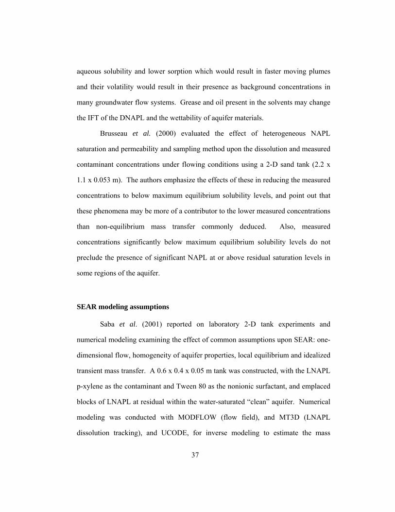
37
aqueous solubility and lower sorption which would result in faster moving plumes
and their volatility would result in their presence as background concentrations in
many groundwater flow systems. Grease and oil present in the solvents may change
the IFT of the DNAPL and the wettability of aquifer materials.
Brusseau et al. (2000) evaluated the effect of heterogeneous NAPL
saturation and permeability and sampling method upon the dissolution and measured
contaminant concentrations under flowing conditions using a 2-D sand tank (2.2 x
1.1 x 0.053 m). The authors emphasize the effects of these in reducing the measured
concentrations to below maximum equilibrium solubility levels, and point out that
these phenomena may be more of a contributor to the lower measured concentrations
than non-equilibrium mass transfer commonly deduced. Also, measured
concentrations significantly below maximum equilibrium solubility levels do not
preclude the presence of significant NAPL at or above residual saturation levels in
some regions of the aquifer.
SEAR modeling assumptions
Saba et al. (2001) reported on laboratory 2-D tank experiments and
numerical modeling examining the effect of common assumptions upon SEAR: one-
dimensional flow, homogeneity of aquifer properties, local equilibrium and idealized
transient mass transfer. A 0.6 x 0.4 x 0.05 m tank was constructed, with the LNAPL
p-xylene as the contaminant and Tween 80 as the nonionic surfactant, and emplaced
blocks of LNAPL at residual within the water-saturated “clean” aquifer. Numerical
modeling was conducted with MODFLOW (flow field), and MT3D (LNAPL
dissolution tracking), and UCODE, for inverse modeling to estimate the mass

38
transfer coefficients (fitting parameters in four empirical Gilland-Sherwood
relationships). Contaminant concentrations in the produced fluid were measured by
gas chromatography and within the sand tank by a dual-gamma attenuation system.
Remediation of sorbed contaminant
Kim et al. (2000) evaluated the use of APU amphiphilic polyurethane nano-
network polymer particles for remediation of sorbed contaminants compared to
surfactants. The model contaminant was phenanthrene. The 1.5 x 20 cm long
columns were packed with sand and contaminant, then flushed with water and APU.
The authors found the following advantages for APU: less adsorption and therefore
higher recovery with less water flushing, less emulsion formation, fewer pv required
for cleanup, high sorbed contaminant recovery efficiency (95%).
SEAR field economics
Ramsburg and Pennell (2001) compared two surfactant formulations for the
planned remediation of a PCE-contaminated site associated with a dry cleaning
business in Oscoda, Michigan, with an emphasis on projected economics for pilot-
scale and field-scale SEAR projects. Two 2-D glass plate cells were constructed and
results were scaled-up for the pilot and field projects using flow simulators. For the
first cell, 8 pv of 4% Tween 80 +500 mg/L CaCl2 were injected for a 53% recovery
of PCE. For the second cell, only 3 pv of 8% Aerosol MA/IPA + 15,000 mg/L NaCl
were injected for a 78% PCE recovery. Site specific soil was used in both cells, with
lower permeability lenses created with finer-grained material. The results from the
two 2-D lab experiments were scaled up to estimate pilot-scale and field-scale

39
project economics, using particle tracking flow simulations and conservative
assumptions for scale-up, such as that contaminant solubility in the surfactant would
be 10% of the theoretical equilibrium value. For pilot scale projects, the authors
estimate remediation would cost $222,000 and $244,000 for remediation by Tween
80 and Aerosol MA/IPA, compared to $316,000 for remediation by conventional
pump-and-treat methods. For field-scale projects the authors estimate remediation
would cost $382,000 and $443,000 for remediation by Tween 80 and Aerosol
MA/IPA, compared to $1,167,000 for remediation by conventional pump-and-treat
methods, for a line-drive pattern, with a substantial reduction in time required (4360
days less for Tween 80). To minimize risk of PCE mobilization, the authors
recommend Tween 80 over Aerosol MA/IPA, where the risk of PCE mobilization
discussed is migration into low permeability lenses or into pristine areas of the
aquifer. The authors saw little benefit in surfactant recycling for the low volumes
required in a pilot-scale project, and estimated savings of 3% of the total project
costs for a full-field remediation project (around $12,000). Risks of recycling
equipment failure or project delays were not included in this evaluation.
Spill event and SEAR 2-D visualization studies
Conrad et al. (2002) used a 2-D heterogeneous sand tank to evaluate and
visualize DNAPL spill events, SEAR, and permanganate in situ oxidation. The 0.6 x
0.6 x 0.01 m tank was packed with sands whose permeability varied by over one
order of magnitude. The DNAPL used was TCE; the surfactants evaluated were
Aerosol MA and Tween 80. Tracer tests were conducted prior to the remediation
experiment to determine the DNAPL saturation. After the spill event, the DNAPL

40
was distributed primarily as a series of high saturation pools on top of the lower
permeability lenses, rather than as a more widely distributed near-residual saturation
often seen in column experiments. 7.3 pv of Aerosol MA solution (1.6% surf., 4%
IPA, 0.3% NaCl) were injected. The authors observed significant DNAPL invasion
into the lower permeability lenses and the underlying aquitard during the SEAR, due
to lowering the IFT of the DNAPL (0.62 dyne/cm). For this reason, the authors did
not conduct a post-SEAR tracer test, believing that injected tracer would not contact
these lenses and that it was “unlikely……a PIT test, would identify this mass as
remaining in the subsurface”. There was less DNAPL mobilization observed during
injection of the Tween 80 surfactant, the IFT was 9.0 dyne/cm, significantly higher
than for Aerosol MA.. 8.6 pv of Tween 80 surfactant were injected. The
contaminant recovered by each surfactant test was not reported (not measured?), as
the purpose of these experiments is visualization of the contaminant migration paths,
and where contaminant resides after remediation is complete.
Surface treatment of SEAR produced fluids
Hitchens et al. (2001) and Abou-Nemeh et al. (2001) reported on VOC
removal from water and surfactant solutions by a pervaporation pilot system for
surface treatment of produced water during a SEAR process. The authors found that
it was possible to separate surfactant without altering its properties, highlighting the
potential for recycling of surfactant to improve the economics of SEAR.
Cheng et al. (2001) reported on another experiment of surface treatment of
produced SEAR fluids: solvent extraction of the contaminant from the
microemulsion using a hollow fiber membrane technology.

41
Severin and Harris (2002) conducted batch experiments to show the potential
utility of detergent/surfactant in a three phase soil washing system to remove PCB
from contaminated soil. The PCB is removed from the surfactant so that surfactant
may be reused for further soil washing, by leaching the PCB with a sacrificial oil
such as vegetable oil (the oil can then be incinerated).
Surfactants and chemical degradation
Li et al. (2002) conducted batch and column experiments to evaluate the
addition of cationic surfactants to increase the degradation of PCE by zero-valent
iron (ZVI) permeable barriers, and found degradation improved by a factor of 5.
Surfactants and biodegradation
Carvalho et al. (2002) conducted batch experiments to evaluate the use of
cosolvents and surfactants to enhance PAH naphthalene bioremediation by
increasing aqueous phase solubility and bio-availability. The authors had mixed
results due to toxicity and biodegradability of these chemicals (ethanol and
Tween80) and emphasize the importance of further research in this area.
Yang et al. (2002) studied biodegradation of phenanthrene in surfactant
microemulsions using batch experiments. Two nonionic surfactants (Tween80 and
Triton X-100) were used as a mixture. This mixture increased the amount of
phenanthrene available for biodegradation in the aqueous phase and did not inhibit
biodegradation, thereby showing the potential of SEAR combined with
bioremediation processes.

42
2.1.3 SIMULATION STUDIES
To date, relatively little attention has been focused on the mathematical
modeling of SEAR field tests . However, these models could play an essential role in
the interpretation of laboratory and field measurements and in the design of effective
field applications. Such models will be necessary to quantitatively integrate and
assess the complex physical and chemical processes affecting the recovery of
entrapped organics. The models of SEAR which have appeared in the literature have
focused primarily on single-phase (aqueous) flow, assuming that recovery of the
entrapped residual is through promotion of micellar solubilization.
The table below summarizes some of the SEAR simulation studies
conducted over the past several decades.
Date Description Simplifying Assumptions
1989, 1991 Wilson, Wilson & Clark: Solubilization of DNAPL by surfactant in an areal model. incl. surfactant adsorption.
2-D, one mobile phase, homogeneous K, equilibrium mass transfer
1993 Abriola et al.: Non-equilibrium solubilization of DNAPL by surfactant
1-D, one mobile phase, homogeneous K
1994 Brown et al.: SEAR in a 2-D and 3-D heterogeneous aquifer with a simple flat aquitard, incl. solubiliz. and mobiliz. of DNAPL. Incl. surf. adsorption. conceptual model only. (UTCHEM)
equilibrium mass transfer, no contaminant adsorption
1996 This research: Field SEAR/PITT in a 3-D heterogeneous aquifer with complex aquitard surface incl. solubilization and mobilization of DNAPL. Incl. comparison with actual field performance. Incl. surf. adsorption. (UTCHEM)
equilibrium mass transfer, no contaminant adsorption
1997 Sabatini et al.: simulation of a single well VCW, vertical circulation well, using the USGS MOC model.
flow field and component tracking model only. no solubilization or mobilization of DNAPL.
1997 Santharam et al.: Biodegradation, surfactant 0-D material balance model, one

43
remediation, and phytoremediation of NAPLS.
mobile phase, equilibrium mass transfer
1998 Ko and Schlautman: Adsorption and desorption of contaminants and surfactants
1-D, homogeneous K, no DNAPL phase (only as sorbed component).
1998 Shook et al.: study of vertical migration and its minimization in SEAR, incl. solubilization & mobilization (TETRAD).
2-D, equilibrium mass transfer, homogeneous K
1999 Finkel et al.: study of SEAR for tar removal using an areal heterogeneous K model (SMART), incl. surfactant and contaminant sorption.
2-D, no velocity changes, equilibrium mass transfer, no DNAPL mobilization.
2000 Dekker and Abriola: study of SEAR for DNAPLs using a 2-D vertical heterogeneous K model (MSURF2D), incl. non-equilibrium mass-transfer.
2-D, no DNAPL mobilization, no surf./cont. adsorption.
2002 Saenton et al.: looked at non-equilibrium solubilization in heterogeneous aquifers for SEAR of LNAPLs.
2-D, one mobile phase, no DNAPL mobilization
2002 Young et al.: design of a SEAR polymer field test for coal tar remediation at Bloomington Ill. by Intera, using a 3-D heterogeneous aquifer model, incl. solubilization and mobilization. (UTCHEM)
2002 Holbert et al. and Meinardus et al.: design of surfactant and surfactant-foam field remediations Hill OU2 for five panels using 3-D heterogeneous aquifer model by Intera Inc.. (UTCHEM)
These simulation studies are discussed in more detail in the text below.
Wilson (1989) and Wilson and Clarke (1991) presented a two-dimensional
areal, single-phase flow model of the solubilization process that assumes local
equilibrium and constant and isotropic permeability of the aquifer. The only
chemistry included in their model was the adsorption of the surfactant and
solubilization of the contaminant. Wilson chose an ionic surfactant, sodium
dodecylsulfate, because it can be recovered by polar solvent extraction and is
“cheap, readily available, relatively nontoxic.” The three NAPL contaminants

44
evaluated were p-dichlorobenzene, naphthalene, and biphenyl. The modeling
technique consisted of two phases: (1) calculation of the flow field and (2)
determination of surfactant movement. Two methods for determining the surfactant
movement were used:
(1) Solve the conservation equation: This is the more realistic but also more
CPU intensive approach. Wilson considered dispersive, advective and
sorptive terms, and neglected biological and chemical reaction terms. Other
assumptions included (a) local equilibrium, (b) a linear function for PCE
solubility vs. surfactant concentration, and (c) an immobile non-aqueous
phase. As an additional assumption, physical dispersion was modeled by
assuming it was equal to the numerical dispersion of the finite difference
approximation of the advection term, with the mesh size adjusted for
consistency with this assumption.
(2) Assume that the surfactant concentration of all streamlines is equal to the
injected surfactant concentration. This simplifying assumption allows
execution of the model on a PC. This method includes all assumptions of the
first method and also assumes that surfactant dilution from the hydraulic
gradient and adsorption may be neglected. The flow field was determined
assuming a constant groundwater flow field, homogeneous thickness and
isotropic permeability, and no permeability reduction due to the presence of
DNAPLs (i.e., the relative permeability effect).
Wilson looked at the sensitivity of the flow field to three variables: (1) the
presence or absence of the hydraulic gradient, (2) the position of the production-
injection axis relative to the flow field direction, and (3) a production rate greater

45
than the injection rate. Calculated surfactant injection times ranged from 5.6 to 16.7
hours to flush the contaminant from a 20x30x1 m remediation volume.
Abriola et al. (1993) present a one-dimensional single-phase flow model of
the solubilization process with special emphasis on rate-limited mass transfer. The
model was implemented in a finite-element simulator and calibrated to laboratory
measurements of dodecane solubilization in soil columns.
Brown (1993) and Brown et al. (1994) presented the results of 3-D
simulations of DNAPL spill events, water flooding, and surfactant flooding in
heterogeneous aquifers, including solubilization and mobilization effects.
Sabatini et al. (1997) conducted a tracer and surfactant vertical circulation
single well test in 1995 at the Traverse City Michigan Coast Guard Station. The
shallow unconfined aquifer was contaminated with PCE and jet fuel but had
undergone a decade of remediation activities and contaminant concentrations were
low. The VCW (vertical circulation well) system was simulated using USGS’s
MOC groundwater flow and solute transport model.
Santharam et al. (1997) presented a simulation study that models surfactant
remediation, biodegradation, and phytoremediation of NAPLs, including NAPL
dissolution, NAPL and surfactant sorption, and the effect of oxygen concentration
upon surfactant and NAPL biodegradation. Also included is the treatment of the
produced flushing surfactant contaminant solution by phytoremediation in which the
solution is sprayed onto a vegetated zone and the contaminant is allowed to
mineralize. Of course, many simplifying assumptions were required to model these
complex processes, including

46
1. The contaminant distribution and the aquifer are homogeneous and the entire zone
is identically flushed by water or the surfactant solution (a 0-D material
balance model).
2. All NAPL is contacted by the surfactant, with equilibrium solubility.
3. The contaminant in not mobilized by the surfactant (solubilization only).
4. The surfactant is biodegradable and does not inhibit/affect the contaminant
biodegradation.
5. The limiting factor for contaminant biodegradation is the oxygen concentration in
the aquifer (all other nutrients are assumed to be available as needed).
6. Only one contaminant compound is present.
7. Only one mobile phase is present, an aqueous phase. No mobile NAPL or oleic
phase surfactant is present.
Pyrene, a DNAPL, was chosen as the model contaminant. The solubility of this
contaminant was increased 130 times by adding 1% Triton X-100 surfactant to the
flushing solution. Hundreds of cases were studied, to examine the effect of
surfactant concentration, oxygen concentration (including air vs. pure oxygen
injection), contaminant and surfactant type, and the number of pore volumes of
flushing liquid required to achieve a final contaminant concentration of 100 ppb.
When combined with biodegradation and phytoremediation, surfactants were found
to have the potential to reduce NAPL remediation time by orders of magnitude
compared to conventional water flushing strategies.
Ko and Schlautman (1998) developed a 1-D simulator to model in detail the
adsorption and desorption of: (1) surfactant upon the subsurface solids, and (2)
contaminant upon the subsurface solids and upon the adsorbed surfactant. The

47
authors report the effect of these phenomena upon SEAR efficiency. A large number
of experimentally determined rate and equilibrium sorption parameters are reported
in this paper, for three contaminants (phenanthrene, naphthalene, and pyrene) and
two surfactants (SDS and Tween 80). The authors found that, under the conditions
simulated, removal of phenanthrene and naphthalene from a sandy aquifer was
actually hindered by adding surfactant to the flushing solution, (by increasing
sorption of the contaminant upon the soil matrix), unlike as expected for more
hydrophobic contaminants such as pyrene, where the use of surfactant enhanced
contaminant removal. Note: Contaminant present as a NAPL was not considered in
this study, only as a sorbed component; therefore, the effectiveness of surfactant in
remediation was wholly dependant upon its sorption/desorption characteristics rather
than its solubilization characteristics.
Shook et al. (1998) examined vertical migration, and its minimization,
during SEAR using three dimensionless scaling groups (RL, Mo, and NG) and four
design parameters. These four parameters can be used to design a remediation with
near-neutral buoyancy, addressing stakeholder concerns about uncontrolled vertical
migration of a contaminant contacted by surfactant, which reduces interfacial tension
and thereby increases contaminant mobility. This neutral buoyancy SEAR, or
SEAR-NB, is critical for remediation in aquifers not underlain by a low permeability
flow barrier. Using the TETRAD simulator, relative vertical migration of the
DNAPL was evaluated over a wide range of the three scaling groups, and graphs
were prepared from the results. These graphs should be very useful as screening
tools and for preliminary design of field and laboratory tests, though the authors
emphasize that site-specific data acquisition and remediation simulation must be

48
conducted prior to any field remediation. The utility of the graphs for predicting
vertical migration was verified by laboratory experiments conducted by the authors
using sand tanks (1 x 0.4 x 0.05 m) and TCE as the DNAPL. The four design
parameters identified as useful for designing SEAR field projects with minimal
vertical migration are:
1. well spacing
2. microemulsion phase density (adding alcohol to injectant)
3. microemulsion phase viscosity (adding polymer to injectant)
4 .injection rate.
Finkel et al. (1999), University of Tuebingen, developed SMART, a
simulator to model surfactant remediation of coal tar. SMART (Streamtube Model
for Advective and Reactive Transport) is a 2-D areal model and includes the effect
of:
1. surfactant micellization above CMC (Winsor Type I system)
2. surfactant sorption on soil
3. contaminant sorption on soil or surfactant/soil
4.increased contaminant solubilization by the surfactant microemulsion
5.heterogeneous permeability and adsorption
Simplifying assumptions included:
1. time-invariant flow-field (no velocity changes during the test and DNAPL
removal does not significantly affect the field)
2. no mass transfer between stream tubes
3. equilibrium mass transfer

49
The streamtubes were calculated using MODFLOW (flow-field) and
MODPATH (particle-tracking). Under the conditions studied, and given the
simplifying assumptions, the authors did not find clean-up efficiently to be
predominantly controlled by large-scale heterogeneity. The authors plan to extend
SMART to model three-dimensional and non-equilibrium sorption.
Delshad (2000) presented a SEAR design a surfactant flood at Camp
Lejeuene, using UTCHEM, to model a 3-D heterogeneous aquifer with extremely
low permeability in the DNAPL area.
Dekker and Abriola (2000) developed a 2-D vertical simulator, MSURF2D,
to model field-scale SEAR processes, including solubilization, permeability and
contaminant heterogeneity, and rate limited mass transfer. The authors used USGS
SUTRA as a basis for the code development, assuming an immobile DNAPL phase,
negligible organic/surfactant sorption upon the sandy matrix (developed for Borden
type soils). The initial DNAPL saturation was obtained by modeling the
contamination event with the M-VALOR simulator. Multiple realizations of the
permeability field for the aquifer were developed, to estimate mean and variances of
output parameters such as volumes injectant required for 50%, 90% & 99.99%
contaminant removal – the authors determined that 15 to 20 realizations were
needed to result in stable mean and variance results. For a 99.9% contaminant
removal, reducing the variance to zero (homogeneous formation) decreased the
cleanup volume by 41%; doubling the variance increased the cleanup volume
required by 72%. The authors also looked at the effect of spatial correlation length
(2.8-8.3 m horizontal and 0.12-0.38 m vertical) and found that, as expected, the
greater correlation lengths resulted in a greater volume of injectant required for

50
cleanup, as well as greater variability in the model predictions, particularly for the
increased variance case. Over the three orders of magnitude range of mass transfer
coefficients explored, there was a relatively small impact upon flushing volumes (7-
11% increase) compared to other parameters, particularly compared to what has been
observed in column experiments. The authors suggest that this is likely due to the
larger dimensions of the spill explored, which result in longer mass transfer zones,
and also that, due to insufficient information, mass transfer coefficient was not
correlated with permeability; such a correlation would be expected to result in a
larger variation in results.
Saenton et al. (2002), of Colorado School of Mines, modeled 2-D non-
equilibrium contaminant dissolution in heterogeneous aquifers for surfactant
enhanced remediation of LNAPL, using the MODFLOW and MT3D simulators and
Gilland-Sherwood empirical correlation models for dissolution of the LNAPL into
the aqueous phase. MODFLOW was used to generate the groundwater flow fields.
Solute transport was simulated with MT3D. The only mobile phase modeled was
the aqueous phase (or aqueous phase microemulsion). Simulations were conducted
for a 91 x 61 cm tank with spills of LNAPL (Soltrol). The authors conclude that
surfactant remediation may result in incomplete delivery of surfactant to low
permeability zones, and therefore achieving cleanup goals may be uncertain. The
authors do not discuss methods to mitigate this risk, such as improving the mobility
ratio and sweep efficiency by the addition of polymer.
Jayanti (2003) evaluated the benefits of reducing DNAPL source mass in
reducing downstream contaminant mass flux and improving groundwater quality,

51
including the effect of contaminant `diffusion from low permeability zones, using
UTCHEM.
Solubilization, however, as noted above, is not the only process which acts
to remove entrapped residuals upon introduction of an aqueous surfactant solution.
The surfactant also tends to reduce the interfacial tension (IFT) between the aqueous
and organic phases, potentially resulting in mobilization of the NAPL as a separate
phase. Indeed, enhanced oil recovery strategies have been based on this process by
promoting the formation of middle-phase microemulsions which lead to ultra-low
interfacial tensions (<10-3 dynes/cm) (Bourrel and Schechter, 1988). Thus, a
general SEAR modeling approach must necessarily be multiphase, taking into
consideration the complexities created by IFT reduction and phase behavior. In
addition, the modeling approach should be multidimensional and permit
heterogeneous distributions of properties, in order to appropriately assess aquifer
conditions present at the field scale.
2.1.4 COMPARISON OF SURFACTANT EOR AND REMEDIATION
Though surfactant EOR and surfactant aquifer remediation both involve the
recovery of an oleic liquid or ‘oil’ by surfactant dissolved in injected water, there are
major differences in these two processes. The goal in surfactant enhanced oil
recovery is to increase oil recovery in order to maximize profitability, with oil
recoveries ranging from approximately 40-70% of that initially in place. The goal in
aquifer remediation is typically to minimize costs rather than maximize profits and
to recover all of the oleic liquid contaminant present (or all practicable), in order to
achieve current regulatory compliance and minimize future site environmental
52
liabilities. This may require removal of up to 99% or more of the NAPL, to achieve
final contaminant concentrations in produced groundwater as low as 5 ppb (0.005
mg/l). Additional differences in surfactant EOR and aquifer remediation include
differences in initial ‘oil’ saturation, aquifer conditions, and surfactant selection
criteria.
In EOR, typically the oleic components' solubility in water is neglected; in
environmental applications the oleic contaminants dissolved in the groundwater have
critical implications for the extent of the contamination (the groundwater plume) and
for determining the oleic mass balance. Permeabilities in petroleum reservoirs are
typically smaller and more heterogeneous than for groundwater aquifers. Surfactant
selection criteria for petroleum applications include cost, thermal stability, hardness
and salinity tolerance, and minimizing the IFT (type III behavior). Surfactant
selection criteria for remediation applications include cost, non-toxicity,
biodegradability, effectiveness in fresh waters, and dominance of either mobilization
or solubilization. Volumes of surfactant injected for remediation applications are
typically much larger, 1-14 pv, than for petroleum reservoir recovery, where the
injected volume of surfactant solution is typically less than 1 pv.
Additionally, wells tend to be shallower and more closely spaced in
environmental applications (1’-50’ deep, 10’-100’ apart) than in petroleum
applications (500’-5000’ deep, 10-100 acre spacing). In environmental applications
the oleic phase contaminant may be crude oil from petroleum reservoirs but may
also be a wide range of chemicals or complex mixtures including LNAPLs such as
gasoline, jet fuel and other refined oil hydrocarbons, and also non-hydrocarbon
DNAPLs such as carbon tetrachloride, TCE, and PCE.

53
Pope and Wade (1995) compared surfactant flooding for environmental and
oil recovery applications and presented lessons learned from petroleum engineering
projects with great potential utility for remediation applications.
2.1.5 APPROXIMATE COSTS OF SURFACTANT REMEDIATION AND SOME REMEDIATION ALTERNATIVES
The maximum total recovery costs acceptable for enhanced oil recovery are
around $0.12-$0.35 for each gallon of oil recovered ($5-$15 per barrel) including the
costs of exploration, drilling, and production. The costs of injected chemicals must
be kept relatively low to meet this constraint. In contrast, the recovery cost for
organic liquid contaminants in groundwater aquifers using the most common
technology, “pump and treat” (primary recovery), is around $400-$4000 a gallon -
$16,000-$160,000 per barrel! Therefore, the acceptable costs (and quantity) of
surfactants used may be much higher for surfactant remediation of groundwater
aquifers than for EOR of petroleum reservoirs. Krebs-Yuill et. al (1995), Fiorenza
et. al. (2000), and Lowe et. al (2000) presented very useful guidelines and case
studies for estimating aquifer remediation costs. NFESC Technical Report TR-
2206-ENV (2002) included useful cost information as well as information on all
aspects of SEAR design and field application.

54
Surfactant Flooding vs. Water Flooding
Years of Remediation
50 75 100 10
100
1,000
10,000
100,000
0.00 0.25 0.50 1.000.75 1.25 1.50
Surfactant Flooding
Water Flooding
Years PV Ratio
Water Flooding 130 442 116
Surfactant Flooding 1.1 3.8 1
Figure 2-1: Comparison of waterflooding and surfactant remediation
However, the primary benefit of surfactants over pump-and-treat remediation
may be time rather than cost: As shown in Figure 2-1, previous modeling work
(Brown, 1993) suggests that adding a carefully designed surfactant injection phase to
a pump and treat program can decrease the cleanup time from decades, or even
centuries, down to a few years or less than a year.

55
2.2 USE OF UTCHEM AQUIFER SIMULATOR IN SURFACTANT REMEDIATION DESIGN
This section briefly summarizes the UTCHEM simulator, describes the
development and use of an aquifer simulation model for studying and designing
aquifer remediations and tracer tests, and examines the effect of some simulated
parameters upon the test design and performance.
2.2.1 INTRODUCTION
UTCHEM is a three-dimensional, multi-component, multiphase (water,
NAPL, microemulsion, air) compositional simulator incorporating higher-order
finite-difference methods with a flux limiter. Use of this simulator makes possible
the study of phenomena critical to surfactant flooding such as solubilization,
mobilization, surfactant adsorption, interfacial tension, capillary desaturation,
dispersion/diffusion, and the complex phase behavior of water /surfactant/ NAPL/
alcohol/ electrolyte mixtures (Delshad et al., 1996; Brown et al., 1994, de Blanc et
al., 1999, Delshad et al., 2000; Wu et al., 2000; Jayanti, 2003).
2.2.2 OVERVIEW OF UTCHEM, THE UNIVERSITY OF TEXAS CHEMICAL FLOOD SIMULATOR
Surfactant enhanced oil recovery models are based upon what is known as a
compositional modeling approach, in which discrete mass balance equations are
solved for each chemical component in the system. In UTCHEM, mass balance
equations are solved for up to nineteen components (water, oil, surfactant, polymer,
alcohol, air, and various electrolytes and tracers). These components can form up to

56
four fluid phases (aqueous, oleic, air, and microemulsion) and numerous solid
phases. A detailed description of UTCHEM modeling capabilities for enhanced oil
recovery has been presented elsewhere (Datta Gupta et al., 1986; Bhuyan et al.,
1990; Saad et al., 1990) and will not be repeated here. Instead, an overview of those
portions of the mathematical model which specifically relate to the presented
remediation design simulations is given below.
Formulation
A mass balance equation for a component k may be written as
[ ] k
n
lkllklkkk QDuCCn
t
p
=⎟⎟⎠
⎞⎜⎜⎝
⎛⎟⎠⎞⎜
⎝⎛
⎥⎦⎤
⎢⎣⎡ −•∇+
∂∂ ∑
=1
~~ rrrρρ (2.2-1)
where n is the porosity, k˜ C is the overall volume of component k per unit
pore volume, klC is the volume concentration of component k in phase l, kρ is the
density of pure component k, and kl˜ D is the dispersion flux of component k in the l
phase, pn .is the number of phases, and kQ is the source term. The phase velocity,
lr u , is given by Darcy's law:
( )hPkku lll
rll ∇−∇•−=
rrrr
r γµ , (2.2-2)
where rlk is the relative permeability, r r k is the intrinsic permeability tensor,
lµ is the viscosity, and lγ is the specific weight ρg( ) for phase l and h is the vertical
coordinate, or depth for the velocity vector.
The dispersive flux is assumed to have a Fickian form given by

57
kl˜ r D = n lS
r r K •
r ∇ klC (2.2-3)
where lS is the saturation of phase l. Here klK is the dispersion tensor,
which is given as (Bear, 1979):
ijklK ≡ klDτ ijδ + Tα
n lSlu + Lα − Tα( )
n lSilu jlu / lu
(2.2-4)
where klD is the diffusivity of component k in phase l; τ is the tortuosity; αL
and αT are the longitudinal and transversal dispersivities; and uil is the component
of the Darcy velocity of phase l in direction i.
A pressure equation can be developed by substituting Darcy's law for the
phase velocity terms in the continuity equation (1), summing over all components
(ncv), and noting that klCk =1
cvn∑ = 1 . The resulting equation can be written explicitly in
terms of aqueous phase pressure (phase 1) as:
n tC∂ 1P∂ t
+r ∇ •
r r k • rTcλ
r ∇ 1P =
−r ∇
r r k
l =1
pn∑ • rlcλ
r ∇ h +
r ∇ •
r r k
l =1
pn∑ • rlcλ
r ∇ cl1P + kQ
k =1
cvn∑
(2.2-5)
where tC is the total compressibility, which is the volume weighted sum of
matrix and component compressibilities, rlcλ is the relative mobility, rTcλ is the
total relative mobility, cl1P is capillary pressure or the pressure difference between
the NAPL and aqueous phases. For incompressible fluids, rlcλ represents the ratio
rlklµ ≡ rlλ and rTcλ = rlλ
l =1
pn∑ .

58
The solution method used in UTCHEM is analogous to the implicit pressure-
explicit saturation (IMPES) method, which is well-established in the petroleum
engineering literature (Aziz and Settari, 1979). First, the pressure equation (2.2-5) is
solved implicitly using a Jacobi conjugate gradient solver, then the mass
conservation equations (2.2-1) are solved explicitly for the total concentration of
each component. Simulations presented herein incorporate three fluid phases, oleic
(organic), aqueous, and aqueous phase microemulsion, and a single solid phase. The
modeled components include organic, surfactant, water, cation, anion, and up to five
tracers. A third-order finite-difference method (Saad et al., 1990) that greatly
reduces numerical dispersion and grid orientation effects is used to solve these
equations. A flux limiter that is total variation diminishing (TVD) (Datta Gupta et
al., 1991) increases the stability and robustness of this third-order method.
Validation of UTCHEM for surfactant enhanced oil recovery field operations can be
found in Saad (1989) and Delshad et al. (1996). A well model is included that
allows for multiphase flow in the injecting and producing wells, either rate or
pressure constraints, and other features standard in the petroleum reservoir
simulation literature (Aziz and Settari, 1979). Aquifer boundaries are modeled as
constant potential and/or closed surfaces.
Phase behavior
In UTCHEM, Winsor Type I, II, and II systems are modeled, as summarized
in the ternary diagram below:

59
.
TYPE II +WINSOR TYPE II
PL
W
S
O
WATER TYPE IIIWINSOR TYPE III
OIL
PL PRM
SURFACTANT
WATER OILTYPE II -WINSOR TYPE I
ELECTROLYTE CONCENTRATIO
N
TEMPERATURE, PRESSURE
SURFACTANT, ELECTROLYTES,
OLEIC TYPE, M
IXTURE
CO-SOLVENTS
SURFACTANT
PR
Figure 2-2: Ternary Phase Diagrams for Winsor Type I, II, and III systems
Phase behavior parameters define the solubility of the organic contaminant
in the microemulsion as a function of surfactant and electrolyte concentrations.
These parameters may be obtained by matching the experimentally determined
solubility for the site contaminant in solutions containing various types and
concentrations of surfactants, co-solvents, and electrolytes.

60
UTCHEM models phase behavior by the Hand equations (Pope and Nelson,
1978). For the microemulsion phase,
c33
c23
= Ac33
c13
⎛
⎝ ⎜ ⎞
⎠ ⎟
B
(2.2-6)
where A is the Hand parameter, determined at various conditions from the
experimental phase behavior data. In these and all subsequent equations, the first
number in the pair of subscripts refers to the component:1=water, 2=contaminant,
3=surfactant. The second number in the subscript pair refers to the phase:
1=aqueous, 2=oleic (NAPL), 3=microemulsion, 4=air. (see Nomenclature section.)
The exponent B may also be determined experimentally; however, UTCHEM
assumes that a symmetrical bimodal curve defines the two-phase region, and,
therefore B = -1:
c33
c23
= Ac33
c13
⎛
⎝ ⎜ ⎞
⎠ ⎟
−1
= Ac13
c33
⇒ A =c33
2
c23c13 (2.2-7)
By definition, the component concentrations in the microemulsion (phase 3)
must sum to 1:
c13 = 1− c23 − c33 (2.2-8)
Combining Eqs. 2.2- and 2.2-8 gives
A =c33
2
c23 1 − c23 − c33( ) 2.2-9)

61
Since the bimodal curve is symmetric (as discussed in text before Eq. 2.2-7),
the maximum C33, C3max, occurs where C23 = C13. Combining this data with a
rearranged Eq. 2.2-8 now results in
c23 = 1 − c3max − c13 = 1 − c3max − c23 (2.2-10)
or
c23 =1− c3 max
2⇒ c3 max = 1− 2c23
(2.2-11)
Substituting Eq. 2.2-11 into 2.2-9 gives
A =2c3max
1− c3 max
⎛
⎝ ⎜ ⎞
⎠ ⎟
2
(2.2-12)
where, for surfactant aquifer remediation applications, these concentrations
are all ‘normalized’ concentrations, adjusted for the oil solubility in water and for the
surfactant CMC, critical micellar concentration. The conversion between
normalized and unnormalized concentrations may be found in Delshad (1989).
To find the concentration for any given electrolyte concentration, UTCHEM
assumes that the Hand parameter A varies linearly between three different salinities:
zero, optimal, and twice optimal, A0, A1, and A2:
A0 =2c3max 0
1− c3 max 0
⎛
⎝ ⎜ ⎞
⎠ ⎟
2
(2.2-13)
A1 =2c3max 1
1 − c3 max1
⎛
⎝ ⎜ ⎞
⎠ ⎟
2
(2.2-14)

62
A2 =2c3max 2
1− c3 max 2
⎛
⎝ ⎜ ⎞
⎠ ⎟
2
(2.2-15)
and:
A = A0 + A1 − A0( ) cse
csopt
for cse ≤ csopt
(2.2-16)
A = A1 + A2 − A1( ) cse
csopt
−1⎛
⎝ ⎜ ⎞
⎠ ⎟ for cse ≥ csopt
(2.2-17)
Interfacial tension
Based on a review of experimental results, Chun Huh (1979) proposed that
the interfacial tension and solubility are intrinsically related by the following simple
function:
2Rc
ow =σ (2.2-18)
where σow is the interfacial tension between the organic and the
microemulsion phases, R is the solubilization ratio, defined below, and c is a
constant.
The UTCHEM correlation for calculating interfacial tension between the
microemulsion phase and the excess phase is based on this simple relationship. In
UTCHEM, this function relates the interfacial tension σl3 and the solubilization
ratio Rl3 :
( )23
3l
l Rc
=σ (2.2-19)

63
where c is a constant typically around 0.20. For an excess aqueous phase
Winsor Type I microemulsion, the phase number is l =1. For an excess oleic phase
Winsor Type II microemulsion, the phase number is l =2 . Rl3 is the solubilization
ratio Rl 3 =
Cl3
C33
, the ratio of the concentration of component l (= 1 for water or = 2
for contaminant) in the microemulsion (phase 3) divided by the concentration of
surfactant (component 3) in the microemulsion (phase 3).
In Eq. 2.2-19, the interfacial tension approaches infinity as the solubilization
ratio approaches zero. To establish a more realistic interfacial tension function, in
UTCHEM the interfacial tension correlation is modified so that σl3 approaches the
oil-water interfacial tension σ21 as Rl3 approaches zero:
σl3 =c
Rl3( )2 Fl 1 − e−aRl 3( )+ σ21e−aR
l 3
(2.2-20)
for l = 1,2 where a and c are the experimental constants and are inputs to the simulator and
F l =1 − e
− C1l − C13( )2 + C2l − C23( )2 + C3l − C33( )2
1 − e− 2for l = 1, 2
(2.2-21)
In the absence of surfactant, interfacial tension reduces to the oil-water
interfacial tension σ21, which, for example, for the site DNAPL and groundwater, is
4.8 dyn/cm.

64
Density
The densities of the microemulsion are determined in UTCHEM from
component densities, using the following relationship:
VT = VS + VA + VW (2.2-22)
where the volume of the total mixture is sum of the pure component
surfactant, alcohol and water volumes or concentrations within the phase.
Phase densities (or specific weights) are calculated in UTCHEM using the
following relationship:
lllllll 332211 γγγγ CCC ++= (2.2-23)
where:
is the specific weight of phase , is the concentration of component 1 (water)
in phase , and is the specific weight of component 1, adjusted for phase
compressibility.
Viscosity
Viscosity in UTCHEM is calculated from the pure component viscosities
and five alpha parameters, with the following equations:
µ 1 = C 11µ w e α 1 C 21 + C 31( ) [ ] + C 21µ o e α 2 C 11 + C 31( ) [ ] + C 31α 3 e α 4 C 11 + α 5 C 31[ ]
µ 2 = C 12µ w e α 1 C 22 + C 32( ) [ ] + C 22µ o e α 2 C 12 + C 32( ) [ ] + C 32α 3 e α 4 C 12 + α 5 C 32[ ]
µ 3 = C 13µ w e α 1 C 23 + C 33( ) [ ] + C 23µ o e α 2 C 13 + C 33( ) [ ] + C 33α 3 e α 4 C 13 + α 5 C 33[ ]
(2.2-24)
l1γl1Cl
l
lγ

65
The microemulsion viscosities calculated by UTCHEM were calibrated to match
measured microemulsion data by adjusting the five alpha parameters.
Rock/fluid interaction properties
Relative permeability
Relative permeability in UTCHEM is modeled by Corey-type functions
(Brooks and Corey, 1966; Pope and Nelson, 1978):
r1k = r1ok n1S( ) 1n
, (2.2-25)
r2k = r 2ok n11 − S( ) 2n
, (2.2-26)
r3k = r3ok n3S( ) 3n
, (2.2-27)
where
n1S = 1S − 1rS( )1 − 1rS − 2rS( )
is the normalized aqueous saturation for imbibition,
and
n3S = 3S − 3rS( )1 − 3rS − 2rS( )
is the normalized microemulsion saturation for
imbibition,
and kr1o , kr2
o , and kr3o are the relative permeability endpoints; n1, n2 and n3,
are the exponents for phase 1 (aqueous phase), phase 2 (DNAPL), and phase 3
(microemulsion phase); and S1r, S2r, and S3r are the aqueous phase residual
saturation, the DNAPL entrapped saturation, and the microemulsion phase residual
saturation, respectively. The influence of IFT upon relative permeability is modeled

66
by making all the above parameters (kr1o , kr2
o , kr3o , n1, n2, n3 , S1r , S2r, S3r) a linear
function of capillary number, which is itself a function of interfacial tension (see Eq.
2.2-29).
Capillary pressure
Similarly to relative permeability, imbibition capillary pressure is modeled
with a modified Brooks-Corey function:
bPcP
⎛ ⎝
⎞ ⎠
λ i
= n1(1 − S ) (2.2-28)
Here Pb is the entry pressure and λi is a curve fitting parameter also known
as the pore size index. Normalized saturations are defined as above for relative
permeability.
The entry pressure Pb in equation (2.2-28) will change as the system
interfacial tension changes. To incorporate this effect in the model, UTCHEM
employs a Leverett function (Leverett, 1941) scaling procedure. Thus, Pb is
replaced by iσ c nk
. Here ci is a curve fitting parameter, σ is the interfacial
tension between the two phases, and k is the geometric mean of the horizontal
permeabilities in the x and y directions. Through this scaling approach, capillary
pressure and relative permeability are modeled as functions of interfacial tension,
porosity, and permeability as well as saturation.
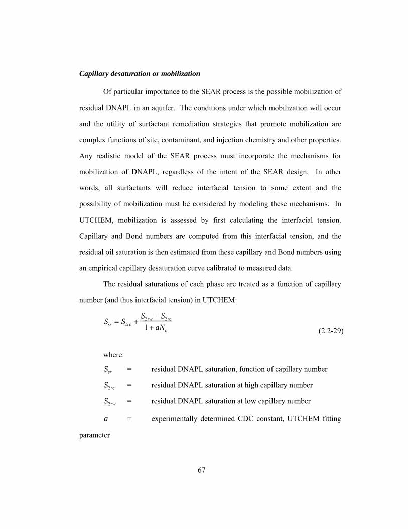
67
Capillary desaturation or mobilization
Of particular importance to the SEAR process is the possible mobilization of
residual DNAPL in an aquifer. The conditions under which mobilization will occur
and the utility of surfactant remediation strategies that promote mobilization are
complex functions of site, contaminant, and injection chemistry and other properties.
Any realistic model of the SEAR process must incorporate the mechanisms for
mobilization of DNAPL, regardless of the intent of the SEAR design. In other
words, all surfactants will reduce interfacial tension to some extent and the
possibility of mobilization must be considered by modeling these mechanisms. In
UTCHEM, mobilization is assessed by first calculating the interfacial tension.
Capillary and Bond numbers are computed from this interfacial tension, and the
residual oil saturation is then estimated from these capillary and Bond numbers using
an empirical capillary desaturation curve calibrated to measured data.
The residual saturations of each phase are treated as a function of capillary
number (and thus interfacial tension) in UTCHEM:
Ssr = S2rc +S2rw − S2rc
1 + aNc (2.2-29)
where:
Ssr = residual DNAPL saturation, function of capillary number
S2rc = residual DNAPL saturation at high capillary number
S2rw = residual DNAPL saturation at low capillary number
a = experimentally determined CDC constant, UTCHEM fitting
parameter

68
Nc = capillary number = σ
Φ∇⋅k
Figure 2-3 shows capillary number values and their effect upon the porous
medium’s residual NAPL saturation, for various experiments and the fit of this data
to the above UTCHEM parametric. Figure 2-4 shows the effect of IFT reduction
alone, for all other variables held constant.

69
Figure 2-3: Effect of capillary number upon residual NAPL saturation
0.0
0.1
0.2
0.3
0.4
0.5
0.6
0.7
0.8
0.9
1.0
1.1
1.2
1E-08 1E-06 1E-04 1E-02 1E+00
Capillary Number .
Res
idua
l DN
AP
L S
atur
atio
n/Lo
w C
apill
ary
Num
ber R
esid
ual S
atur
atio
n
UTCHEM curve for Work Plan Cases 15-25, a=2000
Hill soil & DNAPL, MA surf., 10,000 mg/l NaCl (Oolman et. al, 1995)
Unconsol. Ottaw a 20-30 mesh sand, PCE, MA/AY/OT/W2722 surfs. (Pennell, 1996)
match UTCHEM CDC to Pennell data: a=7000
Sandstone, Decane, petroleum sulfonate surf. (Moh. Delshad, 1990)
match UTCHEM CDC to Delshad data: a = 59074

70
Figure 2-4: Effect of interfacial tension upon residual NAPL saturation
Adsorption
Surfactant adsorption is one of the most important parameters to be
quantified for successful implementation of any field SEAR project. Low values of
surfactant adsorption reduce surfactant quantities needed and hence lower
remediation costs.
Surfactant sorption is modeled in UTCHEM by a Langmuir type isotherm
and is a function of salinity and surfactant concentration:
0.0%
10.0%
20.0%
30.0%
40.0%
50.0%
60.0%
70.0%
80.0%
90.0%
100.0%
0.0001 0.001 0.01 0.1 1 10 100
IFT, dynes/cm
Per
cent
red
uctio
n in
Snr
(am
ount
of D
NAP
L m
obili
zed)
UTCHEM "a" = 7000: unconsolidated Ottawa sand, PCE, W2722/MA/OT/POE20 (Pennell, 1995)
UTCHEM "a" = 59074: Berea sandstone, decane, petroleum sulfonate (Moh. Delshad, 1990)
estimated Hill AFB typical conditions

71
C^
3 = d3b3C31
1 + b3C31 (2.2-30)
where d3 and b3 are experimentally determined parameters, representing the
maximum adsorption capacity and the rate of adsorption divided by the rate of
desorption, respectively. Here the subscript 3 represents the surfactant component
and 1 represents the aqueous phase. The maximum adsorption capacity, d3 is treated
as a linear function of effective salinity in the model. The focus in remediation is
upon recovering the separate DNAPL phase, which contains the majority of the mass
of contaminant within the aquifer, (not recovery of the sorbed phase) and, therefore,
organic sorption was neglected.
2.2.3 EFFECT OF SIMULATION PARAMETERS UPON DESIGN AND PERFORMANCE
The development of an appropriate simulation model is critical to accurate
prediction of remediation performance. This depends not only upon good quality
site characterization and laboratory data but also modeling decisions such as the
number of gridblocks in the model (the mesh refinement), the use of a two-or three-
dimensional model, modeling non-equilibrium phenomena, modeling capillary
desaturation, the number of phases modeled (i.e., inclusion of vadose zone), and the
finite differencing method selected.
The simulation mesh should be fine enough to model the important processes
(consistent with the scale of the variation in aquifer properties and fluids), without
being prohibitively expensive (in terms of computing power, manpower hours, and
elapsed time) to develop, execute, and evaluate. Rather than a globally fine
homogeneous mesh, the degree and location of the mesh refinement may be a

72
function of the type of problem: In LNAPL/unsaturated aquifer cases, where water
table fluctuations and the capillary transition zone have great impact upon predicted
performance, mesh refinement will be most effective in this area of the simulation
model. In DNAPL cases, the mesh can be refined around the DNAPL accumulation
area, and the lower sealing layer of the aquifer, if DNAPL has reached or will reach
this area during remediation.
To determine the effect of mesh refinement upon tracer test performance,
two cases were compared. The Case 12 aquifer model is 16x14x8 mesh with 1792
gridblocks and a gridblock size of 3 ft x 3 ft. x 2 ft. within the test area. The Case 13
aquifer model is a 16x17x9 mesh with 2448 gridblocks and a grid block size of 2 ft.
x 2 ft. x 1 ft.' within the test area, for a gridblock pore volume approximately one
fifth that of the Case 12 model.
Figure 2-5 shows the effect of mesh refinement upon the calculated effluent
concentration for the partitioning tracer, 1-pentanol, in mg/L units. As shown in the
second figure, with a log scale, the refined mesh resulted slightly less curvature at
lower tracer concentrations than in the coarser meshed case.

73
0
100
200
300
400
500
600
700
0 1 2 3 4 5 6
Days
Case 13, refined mesh
Case 12
Figure 2-5: Effect of mesh refinement upon calculated effluent tracer concentration, linear scale
1
10
100
1000
0 1 2 3 4 5 6
Days
Case 13, refined mesh
Case 12
Figure 2-6: Effect of mesh refinement upon calculated effluent tracer concentration, log scale

74
With mesh refinement tracer breakthrough was slightly earlier and peaked at
a slightly higher value. The table below compares the calculated swept volume and
contacted DNAPL volumes from tracer moment analysis for the two meshes:
Case 13, refined mesh
Case 12 difference
DNAPL Saturation: 0.095 0.085 12% greater
DNAPL Volume: 42 ft3 35 ft3 18% greater
Swept Volume: 430 ft3 415 ft3 3% greater
1-Pentanol Recovery: 96% 93%
All values in the preceding table are for 2-propanol / 1-pentanol tracer pair,
for a 5.5 day tracer test with no extrapolation of the concentrations. The mesh
refinement had little effect upon swept volume. Differences in calculated DNAPL
volume may be related to the greater recovery of the partitioning tracer in Case 13
(96% vs. 93% in Case 12). Execution time increased from 4.3 cpu hrs to 13.9 hrs
(CRAY YMP) with mesh refinement, partly due to the 37% increase in gridblocks.
However, the primary cause for the increased execution time is the much smaller
gridblocks for the extraction well completion (pore volume decreased by a factor of
2). Including the 10-day pumping period before the tracer test increased the total
execution time from 13.9 cpu hrs to 20.4 cpu hrs. Note: All CPU times are for
1996 hardware and software. Computer run times in 2004 are substantially less, due
to enhancements in UTCHEM and hardware improvements. In 2004, a 22.4 day
Phase II case required around 1.6 cpu hrs on a 2.4GHz Pentium PC (Delshad, 2004),
in contrast to 9.9 cpu hrs on a Cray in 1996 (Case 39).

75
2.3 MOST IMPORTANT SURFACTANT FLOODING DESIGN PARAMETERS
One of the most valuable uses of a simulation model is as a ‘what if’ tool to
evaluate the effect of many design decisions upon remediation performance. Some
of the most important design parameters, questions and issues include:
• amount and type(s) of surfactant injected
• composition of surfactant solution (type and concentration of added
electrolytes and cosolvents, if any)
• is mobility control (polymer) needed?
• well pattern and well completion design
• injection and extraction rates
• hydraulic control well locations (if any) and rates
• location and frequency of sampling points
• is an electrolyte pre-flush needed?
• design of post-test water flush
• surface treatment facilities
• cost and availability of chemicals
• surfactant toxicity and biodegradability
• percentage of contaminant source removed, under various designs
• effluent concentration peaks of contaminant constituents and injected tracers,
surfactants, salts, and alcohols
• mobilized vs. solubilized contaminant recovery

76
These design parameters are introduced below and discussed in more detail
in Chapter 4: A New Methodology for the Design and Interpretation of Surfactant
Remediation using Modeling. The effects of aquifer and contaminant properties and
uncertainties upon the optimal design are also covered in this chapter.
2.3.1 AMOUNT OF SURFACTANT
The effect of the surfactant injection quantity upon remediation performance
was evaluated, for 1.6 pv, 2 pv, and 2.5 pv injection of a 8% surfactant, polymer,
IPA, electrolyte solution. In the table below, the DNAPL remaining is based upon
tracer test moment analysis of the test area extraction wells. PV Surfactant injected
CaseDNAPL
recovered (gal) DNAPL
remaining (gal) % DNAPL Recovery
1.6
(18,000 lbs of MA-80)
29 455 32 92%
2.0 (23,000 lbs of MA-80)
30 505 20 95%
2.5 (28,800 lbs of MA-80)
31 550 17 96%
As shown in the table above, increasing the amount of surfactant by 28% (2
vs. 1.6 pv) increased the DNAPL recovery by 11% (505 vs. 455 gal); increasing the
amount of surfactant injected by an additional 25% (2.5 vs. 2.0 pv) increased the
DNAPL recovery by an additional 9% (550 vs. 505 gal). This method of
comparison would suggest the point of diminishing returns had been reached for any
additional surfactant over the base case. However, a more useful comparison
parameter is the amount of remaining DNAPL, since minimizing this parameter is

77
the goal of any remediation scheme. The amount of DNAPL remaining decreases by
38% (20 vs. 32 gal) if the amount of surfactant injected is increased by 28% (2 vs.
1.6 pv). The amount of DNAPL remaining decreases by 47% (17 vs. 32 gal) if the
amount of surfactant injected is increased by 38% (2.5 vs. 1.6 pv). The ‘optimal’
amount of surfactant injected will be a function of the remediation objective,
surfactant cost, surfactant / contaminant / groundwater phase behavior, confinement,
aquifer properties such as heterogeneities, and polymer.
If the aquifer is very heterogeneous, inclusion of polymer may greatly reduce
the amount of surfactant required to effectively sweep lower permeability zones of
the aquifer. However, if the aquifer is unconfined (either geologically or
hydraulically) inclusion of polymer may actually decrease contaminant recovery by
resulting in poorer confinement of the injected fluid and lower recovery of injected
fluid and the contaminant it carries. In this as in much else, remediation
performance is very much site specific and therefore the remediation design must be
customized carefully for the site's geology, geochemistry, and contaminant(s)
characteristics.
2.3.2 MOBILITY CONTROL
Case Description Case
Swept Pore Volume, gal
DNAPL remaining (gal)
% DNAPL Recovery
no polymer 33d 11,585 35.6 93.1 %
500 mg/l polymer 36 14,760 30.0 94.9%
Case 33d had 2.0 pv of surfactant injected, no polymer added, a 16.5 day
test, chloride preflush for 1 day before surfactant injection. Case 36 was identical,

78
except polymer was added to the all phases of the test. Swept pore volume is for
final tracer test.
2.3.3 COMPOSITION OF SURFACTANT SOLUTION
Increasing the IPA alcohol concentration in the injected fluid decreases the
amount of salt required to achieve optimal salinity, with an approximately semi-
logarithmic relationship between optimal salinity and % IPA (Figure 6.44 of
Dwarakanath, 1997). Increasing the IPA concentration from 2% to 8% decreases the
optimal salinity from 8,000 mg/l NaCl to 5,800 mg/l NaCl.
2.3.4 WELL PATTERN AND COMPLETION DESIGN
There is an inherent conflict between maximizing site data acquisition and
maximizing well design freedom -- while minimizing project costs. Well data is
needed for accurate simulations leading to a reliable robust remediation designs.
However, if these wells are already drilled in order to acquire aquifer data, then the
well locations and completions cannot be changed during the design process. From
a data/design standpoint, the optimal approach (but most expensive) is to drill test
wells for data acquisition, develop the site characterization, optimize wells during
remediation design simulations, abandon the data wells or use only for monitoring
during the remediation, and then drill completely new wells for surfactant
remediation injection, production, and hydraulic control. However, drilling new
wells after the remediation design simulation also introduces new uncertainties and
may even result in sub-optimal remediation performance, as new wells may have
permeabilities or aquifer thicknesses far different than the design basis or model. In

79
practice, the data wells will be recycled for injection/extraction/monitoring if at all
possible during the remediation to minimize costs.

80
CHAPTER 3: TRACER DESIGN
This chapter focuses on partitioning tracer tests and includes a literature
review, a brief description of tracer test analysis using the method of moments, a
discussion of tracer test design including the most important design variables, and
observations and conclusions regarding tracer design methodology.
3.1 INTRODUCTION AND BACKGROUND
The purpose of a tracer test is to detect and quantify the volume of NAPL, a
discrete, separate nonaqueous contaminant phase. Tracer tests will not detect
contaminant present in the aquifer in the gas, aqueous, or solid phases (vaporized,
dissolved, or sorbed). A great number of partitioning interwell tracer tests (PITTs)
have been conducted since 1994, including LNAPL and DNAPL sites, in saturated
and unsaturated zones, including many tracer tests conducted at Hill AFB, primarily
at the Operable Unit OU1 site, where nine test cells have been constructed to
evaluate different remediation techniques and partitioning tracer tests are used to
determine the amount of NAPL present before and after the remediation (Rao,
1997).
Meinardus et al. (2002) reports on performance assessment for a field
surfactant-foam of a DNAPL contaminated unconfined aquifer at Hill AFB, Utah.

81
The many uncertainties in estimated DNAPL volume, pre- and post-flood, using soil
borings are discussed and compared with those for PITTs. Using soil borings, the
pre-flood DNAPL volume estimate was 74 m 48 l and post-flood DNAPL estimate
was 5.2 m 3.4 l, for a DNAPL volume uncertainty of m 65% for both the pre- and
post-floods. Using PITTs, the pre-flood DNAPL volume estimate was 79 m 27 l and
the post-flood DNAPL estimate was 9.8 m 7.6 l. This represents a m 34% uncertainty
for the pre-flood DNAPL volume and m 78% uncertainty for the post-flood DNAPL
volume. One key finding of this study is that PITTs, properly designed, do not
underestimate the volume of DNAPL, even in this “real world” test where there was
substantial heterogeneity in the permeability and DNAPL distribution. The authors
recommend PITTs for macro-scale NAPL characterization and selective core
sampling for micro-scale NAPL characterization and, in particular, vertical
distribution of the NAPL saturation.
While simulation models are invaluable in the design of tracer tests, the
quality of the simulation is directly a function of the quantity and quality of the site
and fluid data upon which it is based. Therefore, laboratory experiments are of
crucial importance for: screening and selecting the tracers, determining static and
dynamic partition coefficients, and conducting tracer test column floods.
Setarge et al. (1999) report on batch and column laboratory experiments
evaluating four alcohols (IPA, 23DM2B, 4M2P, 24DM3P) and one surfactant
(Marlinat) for use in characterizing coal tar DNAPL volume. Partition coefficients
ranged from 1 to 22. The authors highlight the importance of determining the proper
residence time to achieve equilibrium: decreasing the velocity by a factor of 4

82
increased the mean residence time from 3 to 5 hours and increased the calculated
coal tar saturation 6%.
The following parameters can be usefully predicted by a good quality aquifer
model:
* overall swept pore volume
* degree of hydraulic confinement
* recovery of injected chemicals
* test timing
* breakthrough for the non-partitioning tracers
Parameters that depend upon the amount of DNAPL present, such as
breakthrough of the partitioning tracers, or the degree of separation between tracer
concentration curves, cannot be determined pretest by a simulation model.
However, a series of simulations, with a range of DNAPL present, can be very
useful to “bracket” the possibilities and ensure that the tracer suite design is robust
enough for either high or low volume DNAPL scenarios
3.2 TRACER TEST ANALYSIS
3.2.1 METHOD OF MOMENTS
The DNAPL volume swept by tracers may be determined very simply,
without simulation or inverse modeling, by the method of first moments. The
following analysis assumes steady state conditions (constant injection and extraction
rates), an immobile, invariant DNAPL saturation, equilibrium partitioning (rates low
enough to achieve the minimum retention time determined from laboratory
experiments), and no loss of tracer through volatilization, degradation, or adsorption.

83
These constraints could be relaxed; however, the analysis would be more complex
and the results are likely to be more uncertain.
First, the first moment is determined from the produced tracer concentrations
vs. time data:
2
0
0 s
i
i
it
dtC
tdtCt −=
∫
∫∞
∞
(3.2-1)
where ‘ it ’ is the first moment for the tracer ‘i’, ‘ iC ’ is the concentration of
the produced tracer ‘i’ at time ‘ t ’, and ‘ st ’ is the tracer slug size or time interval
over which the tracer is injected.
The volume of DNAPL swept during a tracer test may be determined by
calculating the difference in the first moments of the tracers. For the case where one
of the pair of tracers dissolves in the aqueous phase only (a nonpartitioning tracer):
Ktt
Mqm
V jn j
12 −=
(3.2-2)
N
N
n
p
SKS
tt
R−
==1 (3.2-2b)
where ‘ jnV ‘ is the DNAPL volume swept by tracers flowing to the
extraction well ‘j’, ‘ q ’ is the flow rate of extraction well ‘j’, ‘ jm ’ is the mass of
tracer recovered by extraction well ‘j’, ‘ M ’ is the total mass of tracer injected by all
injectors in the test area, ‘ 2t ’ is the first moment for the partitioning tracer, ‘ 1t ’ is
the first moment for the nonpartitioning tracer, and ‘ K ’ is the static partition

84
coefficient for the partitioning tracer. The static partition coefficient can be defined
as
K i =Ci, DNAPL
Ci, Water (3.2-3)
where 'K i ' is the partition coefficient of tracer species 'i' and "Ci,DNAPL ' and
'Ci,Water ' are the concentrations of tracer species 'i' in the nonaqueous phase and
aqueous phase, respectively, in units of mg/l.
The theory and applicability of partitioning tracers for estimation of DNAPL
contamination is described by Jin et. al. (1995) and Pope (1994b).
For accurate determination of the DNAPL volume, it is essential to know
very precisely the partition coefficients of the tracers being used, which will vary
with the contaminant, or mixture of contaminants, at the site. The theory and
applicability of partitioning tracers for estimation of DNAPL contamination is
described in detail by Pope et al. (1994), Jin (1995), Jin et al. (1995), and
Dwarakanath et al., (1999). Dwarakanath and Pope (1998) present a method for
estimating partitioning coefficients for alcohol tracers. Jin et al. (2000) and Jayanti
(2003) discuss interpretation and error analysis of tracer tests, including the effect of
aquifer heterogeneity and extrapolation of tracer test data.
Static partition coefficient tests were conducted by V. Dwarakanath (1996)
using DNAPL from the case study site to measure the partitioning coefficients for a
range of alcohol tracers. A total of seven alcohols were evaluated as tracers. The
optimum injection rates in terms of desired retention times for both surfactant and
tracer tests were determined through column experiments. These indicated that a
retention time greater than about 24 hours is needed to achieve local equilibrium,

85
essential for obtaining good estimation of residual DNAPL saturations using
partitioning tracer tests.
3.2.2 EXTRAPOLATION
The tracer response curves should be complete, in order to estimate the
DNAPL volume accurately, because much of the information is contained in the tail
of the response curves, particularly when DNAPL saturations are low and the tracers
have high partition coefficients and, therefore, later, ‘retarded’ arrival times.
Unfortunately, the tracer response curves are often incomplete because time and
budget constraints prevent a tracer test of long duration, particularly when the test
volume is unconfined, as at the Hill OU2 site, which does not have sheet piling
boundaries common in smaller scale tests. The tracer response curves may also be
incomplete due to the dilution of the tracer concentration below the detectable limit
or for other reasons. However, the tails of the tracer response curves can be
estimated by an exponential function, provided the duration of the test is sufficient to
establish this decline (Pope at al., 1994). The first moments of the tracer response
curves can be obtained by dividing the data into two parts. The first part represents
the data from zero to the time tb where it becomes exponential, and the second
covers the exponential part in which it goes from tb to infinity.
After time tb, the tracer response is assumed to follow an exponential decline
given by
C = Cbe− (
t − tba
)
(3.2-4)
where 1/a is the slope of the straight line when the tracer response curves are
plotted on a semi-log scale, and Cb is the tracer concentration at time tb .

86
It can be shown by integration that
Cbe− (
t − tba
)dt = aCbtb
∞
∫ (3.2-5)
and
Cbe− (
t − tba
)tdt = a
tb
∞
∫ (a + tb )Cb (3.2-6)
The first moment ( t ) of the tracer response curve can now be calculated as
t =tCdt + a(a + tb )Cb0
tb
∫Cdt + aCb0
tb
∫ (3.2-7)
3.3 Design and Aquifer Parameters
One of the more valuable uses of a simulation model is as a ‘what if’ tool to
evaluate the effect of design decisions upon tracer test performance. Some of the
most important design parameters and issues include:
• well configuration
• the need for hydraulic control wells; their locations and rates
• injection and extraction rates
• location of well screens and tubing
• location and frequency of sampling points
• number, quantities, and concentrations of injected tracers
• cost and availability of injected chemicals
• required length of tracer test; effect of extrapolation

87
• tracer toxicity and biodegradability
Aquifer characteristics found to be most important in surfactant remediation
and tracer test design and performance:
• interbedded clays and silts
• horizontal permeability
• vertical permeability
• effect of DNAPL distribution (pooled vs. residual DNAPL)
• entry pressure of DNAPL into the low permeability layers, and
corresponding height of DNAPL required for invasion
It has been suggested in` proposals for surfactant remediation that if the low
permeability layers are orders of magnitude lower in permeability, the capillary entry
pressure will probably be too high for the DNAPL to enter the layer. Thus the
permeability contrast that will be the greatest problem will most likely be 3:1 to
10:1. Assuming that the capillary behavior and properties are similar to those of the
Kueper Borden (Kueper and McWhorter 1991) data, the entry pressure for a 55 D
sand is 0.10 psi and for a 7 D sand is 0.28 psi. This would require a thickness for the
DNAPL fluid of 2 inches and 5.4 inches above the zone for entry. (see figure below)
The thickness of the DNAPL accumulations is unknown at Plant 4 and ranged from
10 to 25 feet in the site test area at Hill AFB. Therefore, soil with much lower
permeability (and therefore higher entry pressure) may contain DNAPL at these
sites. Figure 3-1 below shows the TCE/water capillary pressure curve, in inches of
TCE for three permeabilities: the 55 and 7 and 0.55 Darcy. The MS Excel formulae
are also shown to the right of this figure. When the permeability is reduced two

88
orders of magnitude below 55 Darcy, to 0.55 Darcy, the entry pressure is increased
to 1.0 psi, equivalent to a 19 inch column of TCE above the low permeability zone
needed for entry. As the low permeability zones may largely determine the time
required for remediation, they should be included in experiments and simulations of
water flooding and surfactant flooding.
Figure 3-1: Entry pressure, in inches of TCE, required to enter porous media of three different permeabilities
Other aquifer and contaminant characteristics which may be critical in the
proper design of a tracer test to determine NAPL (or even in determining if a tracer
test is an option), many of which were evaluated using these and other simulation
models, include:
• DNAPL composition
• geological structure of aquifer and aquitard
0.0
12.0
24.0
36.0
48.0
0.0 0.2 0.4 0.6 0.8 1.0
Pc, i
nche
s of
TC
E
k=0.55 Dk=7 Dk=55 D
wetting phase saturation
TCE/water Pc, in inches of TCE Formulae:ka = SQRT(kx*ky)Sn1 = (S1_-Sr1)/(1-(Sr1+Sr2))Sn3 = (S3_-Sr3)/(1-(Sr3+Sr2))in units of psi
Pc12 = Cpc*SQRT(ø/ka)*((1-Sn1)^epc)in units of inches of T CE:
Pc12 = Cpc*SQRT(ø/ka)*((1-Sn1)^epc)*18.91 inches

89
• relative permeability and capillary pressure
• composition of both soil and groundwater
• location and seasonal variations in water table
• groundwater temperature; seasonal variations
• presence of a natural hydraulic gradient
• seasonal variations in gradient amplitude or direction
Additional tracer test modeling design and interpretation issues will be
discussed in Chapter 4, A new methodology for the design and interpretation of
surfactant remediation using modeling. Tracer test design observations, conclusions,
and recommended design protocol are summarized in Section 4.6.

90
CHAPTER 4: A NEW METHODOLOGY FOR THE DESIGN AND INTERPRETATION OF
SURFACTANT REMEDIATION USING MODELING
This chapter presents the design and interpretation of surfactant remediation
using modeling, including planning, site characterization, model development, tracer
and surfactant tests design and execution, analysis of the field results, and
comparisons of the predicted simulation results and actual test performance.
Numerous examples from a field trial conducted at Hill AFB and other specific sites
are discussed to illustrate lessons learned and to develop a recommended
methodology for the design and interpretation of tracer test site characterization and
surfactant remediation. Unless otherwise stated, the data and simulations referred to
are from the Hill AFB Phase I and II tracer and surfactant tests conducted in 1996.
Each of the sections below begin with general recommendations and
observations for each major phase of the remediation, followed by a discussion of
specific case examples, to illustrate and support the general recommendations and
observations.
The aquifer simulation model should be developed based on the specific site
characterization and field hydraulic testing; site DNAPL contaminant characteristics;
test array well data, and laboratory experiments using site soil, DNAPL,
groundwater and injected water.

91
Partitioning interwell tracer tests are used initially to estimate the volume of
DNAPL in place and finally to assess the performance of the surfactant remediation.
An extensive program of laboratory experimentation, hydrogeological
characterization, effluent treatment and predictive simulation is critical in the design
of these tests and the success of the project. Simulations are conducted to determine
tracer test design variables such as rates, injected chemical quantities, suite of
tracers, test timing and to predict contaminant and injected chemical recovery,
degree of hydraulic confinement, and pore volume of the aquifer swept by the test
area wells.
From dozens to hundreds of simulation prediction and design parameter
cases may be needed to properly design tests that would achieve the remediation
objectives in the shortest time and at the least cost possible. Design parameters
optimized as a result of the modeling include the well test array, design needed to
achieve hydraulic control, well locations and completion intervals, injection and
extraction rates, location and frequency of sampling points, surfactant quantity,
composition of injected surfactant solution, mobility control with polymer, duration
of water flooding and extraction needed after the surfactant injection, and the
predicted concentrations of contaminants, surfactant, and alcohol in the effluent.
These simulation studies are typically conducted before the site characterization, on
a scoping basis, then after the site characterization for pre-remediation tracer test
design, then after the tracer test for refinements in the remediation design based on
tracer test data and results. Many such iterations may be required over the entire
timeline of the project, from planning to final post-test analyses, but should not be

92
too time-consuming or onerous, if the initial model development results in a robust
and well-characterized simulation model.
In figures in the following sections, field data or experimental data are
typically shown as points and simulation data are shown as smooth curves rather
than discrete points.
4.1 PLANNING
Careful and thorough initial planning sessions are critical to a successful
remediation. Initial sessions should involve all stakeholders, including site owners
and contractors, state and federal agencies, such as DOE, EPA, DOD, TRRC,
TNRCC, etc, and also any other remediation field operators that have current or
future operations near the site. These initial planning sessions should include
determination of:
1. Objectives
2. SWOT analyses (strengths, weaknesses, opportunities, threats)
3. Most important stakeholder concerns and objections
4. Critical constraints or “givens”, such as limitations on costs, time, areas
of operation
5. Project criteria for success, such as contaminant and inj. chemical
recovery, final dissolved concentrations in groundwater, etc.
After the initial planning sessions are conducted, the design process planning
may begin. This should include plans to:
1. begin site characterization and laboratory studies
2. identify test design alternatives

93
3. build simulation model(s) for design evaluation
4. check model quality and validate model with hydraulic conductivity tests
and other field and laboratory data
5. evaluate each alternative’s effectiveness at meeting project objectives,
stakeholder concerns, etc.
6. choose preferred test design
7. predict test performance
8. execute test
9. evaluate test results
10. compare predicted and actual test performance
11. document test results, lessons learned, and recommendations for future
tests.
A field-scale pilot test to remediate DNAPLs using surfactants was
conducted in 1996 at Hill Air Force Base in Utah. The test was divided into two
phases. The rationale for dividing the field test into two separated phases was: (1) to
provide needed additional ‘real field’ performance data before finalizing the design
for the surfactant flood and (2) to address and resolve issues of concern to those
responsible for oversight of the Hill AFB OU2 Site. One of these concerns was that
the injection of solutions containing surfactant could result in gel formation or other
unfavorable phase behavior that might lead to pore plugging, decreased aquifer
hydraulic conductivity, decreased well productivity and injectivity, and increased
trapping of contaminants within the aquifer, resulting in the very opposite of the
tests’ objective — increased contaminant removal. Another concern was that the
decision not to use sheet-piling boundaries would result in a lack of hydraulic

94
control, migration of microemulsions containing high concentrations of dissolved
contaminants outside the test array, poor recovery of the injected chemicals, and
high remaining concentrations of injected chemicals remaining in the aquifer after
the tests’ completion. The Phase I test was designed to resolve these concerns
before the Phase II test’s injection of large quantities of surfactant into the test area.
The objectives for the pre-remediation tracer test are typically to:
(1) determine the amount of DNAPL initially present with tracers,
(2) achieve and demonstrate hydraulic control,
(3) determine the swept volumes with tracers,
(4) measure hydraulic conductivity before surfactant injection,
(5) test the surface treatment facilities,
(6) test the subsurface injection-extraction well equipment,
(7) validate tracer selection and performance,
(8) validate well patterns and locations, and
(9) optimize the onsite sampling and analysis procedures.
The pre-remediation tracer test consists of an initial water flushing segment,
tracer injection, water flushing, and final post-test extraction to recover any
remaining injected chemicals. Water flushing consists of injection of water only to
move the fluids within the test array aquifer volume (consisting of injected water,
dissolved and/or separate phase contaminant, groundwater, injected chemicals)
through the test area and towards the extraction wells where they are pumped and
treated at the surface.
The objectives for the surfactant remediation test are typically to:
(1) remove essentially all DNAPL in the swept volume,

95
(2) achieve a final DNAPL saturation of below the success criterion (for
example, final DNAPL saturation of 0.001 or 0.1%), and
(3) maintain hydraulic control.
In addition to these objectives, the initial project planning sessions may
result in project “givens” or constraints, such as:
(4) completion of the test within a certain amount of time, (for example, 30
days)
(5) use of only biodegradable chemicals, and
(6) use of only the existing surface treatment facilities on site.
The surfactant remediation phase typically consists of an initial water
flushing segment, tracer injection, water flushing, chloride injection, surfactant flood
with surfactant/alcohol/chloride/(polymer) injection, water flushing, tracer injection,
water flushing, followed by post-test extraction to recover any remaining injected
chemicals. A tracer test may not be required for this phase, if the well pattern and
locations are not changed, and the site remains exactly the same as when the initial
tracer test was conducted.
The objectives for the post-remediation tracer test are typically to:
(1) accurately assess remediation performance by determining the amount of
DNAPL remaining after remediation,
(2) achieve and demonstrate hydraulic control,
(3) determine the post-remediation swept volumes,
(4) measure hydraulic conductivity after surfactant injection,
(5) recover all the injected chemicals, and
(6) measure low final concentrations of all injected chemicals.

96
The post-remediation tracer test phase typically consists of water flushing,
then tracer injection, followed by water flushing, ending with additional extraction to
recover any remaining injected chemicals.
An example timeline for a surfactant remediation project is the three years
required from project initiation to final report for the tests at Hill AFB. The timing
and steps for this project were:
• project planning, including initial discussions, preliminary proposal
submission and approval, 1994 and first half 1995
• data gathering and development of the initial workplan, first half 1995
• preliminary tracer and surfactant simulations, Sep. - Dec. 1995
• site characterization, test well drilling, and laboratory experiments,
second half of 1995
• pre-test DNAPL pumping, late Oct. & early Nov. 1995
• cased hole logging, late Nov. 1995
• hydraulic testing, early Dec. 1995
• simulation model development, Jan. 1996
• tracer and remediation tests design, Feb. & April 1996
• Phase I Test Field Execution (pre-tracer test and test surf. injection),
April & early May 1996
• analysis and interpretation of the Phase I test, May & June 1996
• Phase II surfactant remediation test design refinements, June & July
1996
• Phase II Test Field Execution (surfactant remediation and final post
tracer test) Aug. & Sept.1996

97
• analysis and interpretation of the Phase II test, including additional post-
test simulations and preliminary documentation, Oct. 1996 – Dec. 1996.
• documentation and Final Project Report, Jan.1997 – Aug. 1997.
4.2 SITE CHARACTERIZATION AND LABORATORY STUDIES
Most critical to the design of a surfactant remediation test that will
successfully meet its objectives is a thorough knowledge and understanding of the
characteristics of the site and the contaminant and the behavior of various tracers and
surfactants interacting with site soil, contaminant, and groundwater and injection
water and their constituents. Extensive field data acquisition and laboratory
experiments are essential in gaining this knowledge. One of the best tools for
synthesis of these many disparate data is the use of simulation, which, used properly,
allows evaluation of the effect of different design parameters and data uncertainties
upon remediation performance.
The site characterization includes the following steps: reviewing site history,
hydraulic testing and well logging, development of the geologic model, DNAPL
characterization, phase behavior and column laboratory experiments, surface
treatment simulation and bench testing.
4.2.1 SITE HISTORY AND TEST ARRAY WELL DESCRIPTION
From 1967 to 1975, spent degreaser solvents and other chemicals were
disposed of in two shallow unlined earthen trenches at the Hill Air Force Base

98
Operable Unit 2 (Hill AFB OU2), formerly Chemical Disposal Pit #3, located north
of Salt Lake City, Utah. These disposal trenches allowed DNAPL to drain into an
alluvial aquifer confined on its sides and below by thick clay, resulting in the
formation of a DNAPL pool. The DNAPL at this site consists primarily of three
chlorinated solvents or VOCs (volatile organic compounds). These are
trichloroethene (TCE), 1,1,1-trichloroethane (1,1,1-TCA), and tetrachloroethene
(PCE).
After high concentrations of TCE were discovered downstream of this site,
Radian installed the SRS, Source Recovery System, consisting of extraction wells
and surface treatment facilities, to recover DNAPL and contaminated groundwater.
From October 1993 to June 1994, 23,000 gallons of DNAPL and over 1,000,000
gallons of contaminated groundwater were produced from these wells (Radian,
1994a). This still left much DNAPL source remaining at the site in the form of
residual or bypassed DNAPL not recovered by pump and treat operations that will
continue to contaminate the groundwater. In September and October of 1995, Intera
drilled the test array well borings, SB-1 through SB-8 in the OU2 area. In
November 1995, approximately 550 gallons of DNAPL were pumped from these
wells. As part of the site characterization process, in November and December of
1995, hydraulic testing and natural gamma logging were conducted for these wells.
In April and May of 1996, the Phase I test was conducted. In August and September
of 1996, the Phase II test was conducted.

99
SB-1
U2-201
U2-638
SB-5
SB-6
SB-3SB-2
SB-4
SB-8
SB-7
U2-637
N
0 20 40
Approximate Scale, ft.
U2-1
Extraction wellInjection wellHydraulic control wellTest monitor wellMonitor well
Figure 4-1: Site Plan View
Figure 4-1 shows the site and the locations of the test array wells and nearby
wells. Within the test array, there are a line of extraction wells (U2-1, SB-1, SB-5)
to the north 10 feet (3.1 m) apart and a line of injectors (SB-3, SB-2, SB-4) 10 feet
(3.1 m) meters apart and located 18 feet (5.4 m) south of the line of extractors. This
20 ft by 18 ft (6.1 m x 5.4 m) approximately square test array well configuration is
also referred to as a 3x3 line drive pattern. A monitoring well, SB-6, is located in
the center of the test array. An hydraulic control well, SB-8, is located 18 feet (5.4
m) south of the line of injectors. The injectors within the test array inject water and
various chemicals while the hydraulic control well is located outside of the test array
and injects water only. Water samples were taken from monitoring wells U2-631

100
and U2-33 to the north and south of the test array, respectively. Additional fluid
level monitoring wells are located to the north and south of the test array. The site’s
two abandoned chemical disposal trenches, used for disposal of spent degreasing
solvents, are believed to be located above and slightly to the south of U2-1; the exact
location is unknown. The approximate orientation of the two parallel disposal
trenches is estimated to be running from north-northwest to south-southeast, with
dimensions of 10 feet (3 m) wide by 6 feet (2 m) deep by 10 and 100 feet (15 and 30
m) long, and about 25 feet (8 meters) apart (Radian, 1993; Intera, 1996).
4.2.2 AQUIFER CHARACTERIZATION
The uppermost shallow unconfined aquifer at the site is of limited areal
extent and is located in a deltaic depositional environment, on the edge of a landslide
complex. This aquifer is in the Pleistocene Provo Formation, composed primarily of
discontinuous lenticular gravels and sands, with occasional occurrences of
interbedded silts and clays. Underlying the Provo is the Pleistocene Alpine
formation, several hundred feet thick and composed primarily of layered clays with
occasional stringers of coarser grained material. Underlying the Provo are two
deeper confined aquifers. The water table for the shallow aquifer is approximately
20 feet (6 m) below ground level. (Intera, 1996)
The regional hydraulic gradient in the Provo Formation unsaturated aquifer
is largely controlled by the topography of the aquitard and the stratigraphy resulting
from the landslide processes that formed the aquifer. Groundwater flow is towards
the northeast and may be as high as 0.08 to 0.20 in areas of the aquifer with high
topographic relief, varying in direction and magnitude seasonally. Where the aquifer

101
channel is much flatter, however, as in the test array, the hydraulic gradient is much
smaller. In the test area the hydraulic gradient is around 0.002 (Radian 1994a), with
water entering the aquifer in the test area by (1) flowing down the sloping ground
surface to the west of the test area and percolating through the unsaturated zone and
(2) from the regional natural hydraulic gradient, entering the test array from the
southeast. The natural hydraulic gradient is approximately two orders of magnitude
less than the artificial gradients induced during the field tests.
Structure and Sedimentology
Figure 4-2 is a contour map of the aquitard underlying the aquifer and
bounding it to the east and west. North is pointing to the top of the figure. This
aquitard structure map was developed by Hans Meinardus of Intera in January 1996
and is based upon earlier regional structure maps, drilling logs, and gamma logs.

102
Figure 4-2: Hill AFB OU2 Aquitard Structure
Depth to the water table (approx. 4667' AMSL, above mean sea level) is 20
feet to 25 feet below ground surface in the U2-1 area and varies substantially
throughout the year due to rainfall variations and operation of the source recovery
system. For example, the water table was approximately 4655' AMSL in March
1996, for a saturated zone thickness at Well SB-6 of only 8 feet. The source
recovery wells were shut-in a few weeks before the Phase I test and the water table
rose 12 feet, to 4667’ AMSL, for a maximum saturation zone thickness of 20 feet (at
Well SB-6). The thick contour line to the east and west of the test array indicates an
estimated contour line for the 4667' AMSL depth of the aquitard, the Alpine
Formation, underlying the aquifer.
U2-1 SB-1 SB-5
SB-6
SB-3 SB-2 SB-4
SB-8
"Wet Season" Water Table DepthApproximate Depth to DNAPL "Pool"Test Area WellsPumping and Monitoring Wells
Legend:
Contour Interval: 2 ft

103
This map of the aquitard structure changed substantially from the time of the
study planning stages to the time the SB series of wells were drilled. The north to
south trend of the aquifer was known but the east to west extent of the saturated zone
was very uncertain. For example Well SB-7 (Figure 4-1) was originally intended as a
downstream monitoring well. However, during drilling of SB-7, no saturated zone
was encountered; the aquitard was reached at 4680’ AMSL, 13 feet above the 4667’
AMSL water table. The Alpine Formation is on the order of several hundred feet
thick and bounds the aquifer below and to the east and west by a very steeply
dipping structure, ranging from 30° to 60° dip angle, and results in the north to south
trend of this unconfined alluvial aquifer. The deepest part of this aquitard also
determines the probable migration path of the DNAPL contaminant. Once the
DNAPL migrated downwards from the disposal trenches to the aquitard (or any zone
of sufficiently low permeability above the aquitard), it migrated down slope along
the channel. DNAPL pools have been detected both to the north and to the south of
the disposal trenches. The 4650’ contour (shown as the figure 8 type double lobed
blue contour line) represents the depth of the DNAPL pool discovered in 1993. The
larger northern lobe of the pool was pumped and the more mobile DNAPL recovered
by the source recovery system in 1993 and 1994. The southern lobe of this DNAPL
pool is in the Phase I&II test area and the more mobile DNAPL was recovered from
this section by pumping in December 1995.
The test array wells are labeled in the Figure 4-2 map (shown in red). Other
wells are shown as unlabeled dots (green). The light gray lines are two foot contour
intervals representing the structure of the Alpine formation, the base of the aquifer.
The 4667’ blue contour interval is the depth of the water table in April 1996 and,

104
therefore, demonstrates the maximum extent of the saturated zone at the beginning
of the Phase I test, around 60 feet in width from east to west. In drier seasons or
when the source recovery system is operating, the areal extent of the aquifer zone
would be substantially less. These aquitard contour intervals are based on rather
sparse data, particularly at the east and west boundaries, and there is substantially
more uncertainty in these contours than through the central channel of the aquifer.
Figure 4-3 is a key to the five cross-section figures, Figure 4-4 to Figure 4-8. The
areal locations of sections AA’ through DD’ are indicated in the plan view on the
left. In this plan view, the three test array extraction wells are indicated by solid
circles with arrows pointing upward (red in color versions), injection wells are
indicated by solid circles with arrows pointing downwards (green for test array
injection wells and blue for the hydraulic control well in color versions). Well SB-6,
in the center of the test array, is a monitoring well (lilac in the color versions). The
sedimentology, the key on the right side of Figure 4-3, was estimated from drilling
cutting descriptions or from examination of cores. In general, lighter patterns
represent media with larger particle size and higher permeability while darker
patterns represent smaller particle sizes and lower permeability zones of the aquifer,
with the solid blocks representing vertical sections where clay or silty clay was
encountered. The water table depths at various times are shown on the cross-
sections as a date above an open triangle resting upon a blue horizontal line.
Likewise, depths to DNAPL encountered in wellbores are represented by a date
above a closed triangle resting upon a red dotted horizontal line.

105
Silty Sand orClayey Sand
Clay or Silty Clay
Silt or Clayey Siltor Sandy Silt
SandGravel orSandy Gravel orGravelly Sand
InterbeddedSilt/Clay/Sand
Water Table LevelDNAPL Level
LITHOLOGYPLAN VIEW OF CROSS-SECTION
SB-8
SB-4
approx. scale, in feet
0 20 40
N
U2-1SB-6
SB-7
U2-637
U2-638
U2-201SB-5
C
B'
D
A
B
A'
D'
SB-3
Extraction Well
Test Area Monitoring WellHydraulic Control Inj. WellInjection Well
SB-2
SB-1
C'WELL SYMBOL KEY
Figure 4-3: Plan view of cross-sections of test area and lithology key
Figure 4-4 is a west to east cross-section through the three extraction wells U2-
1, SB-1, SB-5, and well boring SB-7. Vertical depths are to scale while horizontal
distances between wells are not shown to scale in this and the other cross-section
figures. The SB-7 boring, located 40 feet to the east of SB-5, encountered no sand;
the revised aquifer model, with a saturated zone ending 20 feet to the east of SB-5, is
consistent with this. The solid blue line at 4667’ AMSL represents the water table
used in this design study. Previous studies (Oolman, 1995; Jin, 1995) assumed a
water table depth of 4670’ AMSL, based on characterization knowledge current at
that time. Fourteen feet below this 4667’ line, the red dashed line at 4653’ AMSL
represents the top of the DNAPL “secondary pool” contaminated zone used in these
design studies (4650’ AMSL used in previous studies). The sand packed interval

106
(gray-shaded rectangle) and screened interval (striped rectangle within gray-shaded
rectangle) are indicated by rectangles to the right of the depth scale for each well
boring. For example, Well SB-1 is sand-packed from 4660’ down to 4647’ AMSL
and screened over the lower 10 feet of this interval, from 4657’ to 4647’ AMSL.
The depth to the clay aquitard (lower extent of the aquifer) is highlighted by a thick
gray line connecting the top of the clay in each well. This aquitard depth was
estimated by Hans Meinardus of Intera by evaluating all the data available: gamma
logs, well cuttings, and cores and DNAPL levels where available.

107
4670'
4660'
4650'
4640'
4680'
4690'
U2-1
EAST
WEST
8
7
6
5
9
8
7
6
5
9
SB-7
?10/95
SB-1
9/95
8
7
6
5
9
8
7
6
5
9
SB-5
WEST
4/5/96
4/15/96
approx. 10 feet approx. 10 feet approx. 40 feetAA'
17° dip41° dip
34° dip
?
?
?
?10050 10050
10050
Figure 4-4: AA’ west->east stratigraphic cross-section through Well U2-1
8
7
6
5
9
SB-4
8
7
6
5
9
10/95
WEST EAST
4670'
4660'
4650'
4640'
4680'
4690'
9/95
9/95
8
7
6
5
9
4/5/96
4/15/96
B B'approx. 10 feet
10050
10050
44° dip
16° dip
SB-2SB-3 approx. 10 feet
Figure 4-5: B-B’ west->east stratigraphic cross-section through Well SB-2
Most wells have a 15 to 25 feet thick gravel zone above this aquitard, which
would result in a high hydraulic conductivity for the aquifer. Well SB-1 shows

108
approximately 2 feet of finer grained material (sand) between the gravel and the
aquitard. There are question marks over the Well U2-1 sedimentology because this
well was drilled several years ago, before the SB series of wells, and no core was
obtained for this well. Hence, there is considerable uncertainty in the depths and
sedimentology descriptions of cuttings recorded in the drilling log for this well.
Given the uncertainty of the depth to the aquitard for U2-1 and, to a lesser extent, the
SB series of wells and the critical importance of the aquitard in both the probable
migration path of the DNAPL and subsequent distribution and the performance of
the remediation, an accurate determination of the structure of the aquifer (and the
depth to the aquitard) was essential. Early simulations conducted in September 1995
with a flat test area structure showed a substantially different performance.
For this reason, the wells were logged in late November 1995, between the
DNAPL pumping in early November 1995 and the hydraulic testing in December
1995. Because the wells had been completed for extraction, a cased hole technique,
natural gamma logging, was used. In this technique, the fluctuations in the natural
gamma radiation of the formation as a function of depth down-hole is measured and
recorded. In sedimentary formations such as those at OU2, the magnitude of the
gamma radiation measures the clay content of the formations, because shale and
clays concentrate the naturally occurring radioactive elements, such as potassium,
uranium, and thorium isotopes. In general, the average depth of penetration of
gamma rays is around a foot, an indication of the sampling radius of this logging
technique (Schlumberger, 1972). The gamma logs are shown in Figure 4-4 through
Figure 4-7, to the left of the sedimentology. Low gamma radiation intervals (low
amplitude measurements, nearer the left side of the gamma log) indicate higher

109
permeability formation containing fewer clays, such as sands and gravels. Higher
gamma radiation intervals (high amplitude measurements, nearer the right boundary
of the gamma log) indicate aquifer containing shales and clays, with typically lower
permeability. There is an artificially high gamma peak shown on these logs at the
depth of just above the sand packs, which are sealed with 2 - 4 feet thick plugs of
bentonite (clay containing small amounts of naturally occurring radioactive
minerals) slurry atop the pack. For example, Well SB-5 has a two foot bentonite
plug placed from 4667’ to 4669’ AMSL, and the highest gamma ray peak for this
well is from 4666’ to 4670’ AMSL. This type of completion confirmation in the
logs may be useful for depth cross-validation.
Based on these logs, the depth to the bottom of the aquifer is at 4657.6’
AMSL at Well U2-1 and drops 8.8 feet vertically downwards to central extraction
Well SB-1, which is only 10 feet east, for a dip angle of 41°. This dip should be
considered an average and estimate only, as the aquitard is, of course, not a straight
plane between wells but rather a complex undulating boundary with variable slope
and intervening ‘dimples’ and ‘bumps’. The western extraction Well SB-5, 10 feet
east of SB-1, dips upwards 3.1’, for a dip angle of 17° (Figure 4-4). Well SB-7,
located 40 feet to the east of Well SB-5, encountered the aquitard at 4679’ AMSL,
which is 27.1 feet shallower than at SB-5, for an average dip of 34° (Figure 4-1).
These very high dip angles, ranging from 17° to 41°, illustrate the high degree of
confinement in the saturated zone aquifer to the east and west of the aquifer in the
test array.
This cross-section AA’ (Figure 4-4) also demonstrates the importance of the
water table level in the performance of any tracer test or remediation trial. When the

110
water table dropped from 4667’ AMSL down to 4655’ AMSL, as it did in March
1996, there was no water at all in the Well U2-1 wellbore, and only a few feet of
saturated sand at the extraction wells SB-1 and SB-5, which would have been
reduced further once the wells began pumping and would of course substantially
decrease the wells’ productivity and sustainable rates.
Figure 4-5 is a west to east cross-section, BB’, through the three test array
injection wells SB-3, SB-2, and SB-4. The channel structure for these three injectors
is similar to that for the three test array extraction wells of the previous cross-
section, AA’, where the central well is deepest, the western well is shallowest, and
the eastern well is located between. Once again, the greatest dip is between the
eastern well and the central well, suggesting that the western edge of the test array is
closer to the ‘wall’ of the aquifer channel and the eastern edge of the test array is
farther from the wall of the channel.
Figure 4-6 is a north to south cross-section through the center of the test array,
passing through the extraction Well SB-1, the monitoring well SB-6, the test array
injection Well SB-2, and the hydraulic control well SB-8. In contrast to the previous
two cross-sections across the channel, this cross-section is along the axis of the
aquifer channel, and the slope of the aquitard is much flatter The aquitard for
extraction Well SB-1 is at 4648.8’ AMSL and drops only 1.9 feet to monitoring
Well SB-6, located 10 feet to the south, for a dip of around 11° downwards. The
aquitard at Well SB-6 is deepest of all the test array wells. At injection Well SB-2,
located 10 feet to the south of Well SB-6, the aquitard is 0.7 feet higher, for an
average dip of only 4° upwards. The aquitard at the hydraulic control Well SB-8, 20
feet to the south of SB-2 is 2 feet shallower, for a dip of 6° upward. The aquitard

111
slopes downward from SB-1 to SB-6 and then slopes gently upward from SB-6 to
SB-2 to SB-8.
4/5/96
10/95
8
7
6
5
9
SB-6
4/15/96
9/95
9/95
8
7
6
5
9
SB-2
9/95
8
7
6
5
9
4670'
4660'
4650'
4640'
4680'
4690'
8
7
6
5
9
SB-8
4/5/96
4/15/96
4/5/96
4/15/96
SOUTH
C C'approx. 10 feet approx. 10 feet
11° dip 4° dip
10050 100501005010050
6° dip
approx. 20 feetSB-1
NORTH
Figure 4-6: C-C’ north->south stratigraphic cross-section through Well SB-1

112
8
7
6
5
9
4/944670'
4660'
4650'
4640'
4680'
4690'
8
7
6
5
9
U2-637
4/94
5
8
7
6
9
11/94
U2-201NORTH
A'SOUTH
U2-1
8
7
6
5
9
4/5/96
4/15/96
8
7
6
5
9
10/95
SOUTH
U2-638 D'D SB-3
?
?
?
?
approx. 16 feet approx. 7 feet approx. 15 feet approx. 3 feet
Figure 4-7: D-D’ north->south stratigraphic cross-section through Well U2-1
Figure 4-7 is a north to south cross-section through the western edge of the test
array, passing through Wells U2-201 and U2-638, the test array extraction Well U2-
1, Well U2-637, and the test array injection Well SB-3 (see Figure 4-3). Well U2-201
has only around 7 feet of sand in the saturated zone between the aquitard and the
water table. As shown in this cross-section figure and the three previous figures,
most wells have finer-grained, less permeable zones (silt/clay) in the upper
unsaturated aquifer and higher permeability zones (gravel/sand) in the saturated
zone, between the water table (thin solid blue line) and the aquitard (thick gray line).
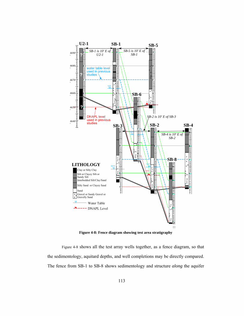
113
10/95
8
7
6
9
SB-2
5
9
8
7
6
5
SB-4
SB-4 is 10' E ofSB-2
SB-89/95
9/95
SB-2 is 10' E of SB-38
7
6
5
9
8
7
6
9
SB-3
5
10/95
SB-1
8
7
6
5
9
9/95
SB-5
8
7
6
5
9
?
SB-5 is 10' E ofSB-1
DNAPL levelused in previousstudies
U2-1
8
7
6
5
9 SB-1 is 10' E ofU2-1
water table levelused in previousstudies
SB-6
Silty Sand or Clayey Sand
Clay or Silty ClaySilt or Clayey Silt orSandy Silt
SandGravel or Sandy Gravel orGravelly Sand
Interbedded Silt/Clay/Sand
LITHOLOGY
Water TableDNAPL Level
9
8
7
6
5
4670'
4660'
4650'
4640'
4680'
4690'
?
?
?
?
Figure 4-8: Fence diagram showing test area stratigraphy
Figure 4-8 shows all the test array wells together, as a fence diagram, so that
the sedimentology, aquitard depths, and well completions may be directly compared.
The fence from SB-1 to SB-8 shows sedimentology and structure along the aquifer

114
channel and the fences going from U2-1 to SB-5 and SB-3 to SB-4 likewise show
sedimentology and structure across the aquifer channel. A few feet of finer-grained
material occurs just above the aquitard in four of the seven test array wells. In Wells
SB-1 and SB-3 this is a sand interval and in Wells SB-6 and SB-4 this is a silty sand
interval. This finer grained material may serve as capillary traps for DNAPL and
increase the resistance to flow for fluids entering the wellbores from this zone. This
finer grained material was not modeled as a specific geologic layer in the
simulations, as it was discontinuous and is believed to be lenticular rather than
layered (Intera, 1997).
Further information on the characteristics of Hill AFB Site OU2 may be
found in Radian (1994a), Oolman et al. (1995, Intera (1996), and Intera (1997).
Hydraulic testing
Many pumping tests have been conducted in the field over the past eight
years and measured hydraulic conductivities ranging from 3.5x10⁻⁵ to 4.1x10⁻⁴ m/s,
equivalent to 3.6 to 44 darcy for an aquifer containing only water at normal density
and viscosity. Hydraulic conductivity and permeability are related in the following
manner:
(4.2-1)
Analysis of U2-1 pumping tests conducted in 1988 yield conductivities
ranging from 3.5x10⁻⁵ to 1.4x10⁻⁴ m/s (equivalent to 3.6 to 15 darcy). Analysis of
U2-1 pumping tests conducted in 1994 yields conductivities from 1.5x10⁻⁴ to 4.1x10-
w
wrw gkkKµ
ρ=

115
4 m/s (16 to 43 darcy). (Radian, 1994). Hans Meinardus of Intera has suggested that
the increases in conductivity observed from 1988 to 1994 may be caused by a
decreasing DNAPL saturation, which would increase the water relative permeability
due to less pore blocking/interference effects and, therefore, would increase the
observed hydraulic conductivity, though the absolute permeability remains
unchanged.
Determining realistic in situ properties for unconsolidated samples can be
very difficult, due to rearrangement of the grains and disruption of the porous media
during boring, transport, cutting, and storage. The difficulty is increased for the site
samples because the aquifer is composed primarily of gravel interspersed with
cobbles, some of them larger than the 6 cm diameter sampling tube. To minimize
the core disruption, the sampling tube was frozen upon reaching the laboratory,
before core cutting and until the measurements could be obtained. TerraTek Inc.
(1994) measured permeabilities from the Hill AFB OU2 site (just north of the test
array) for five soil samples which ranged from 3.9 to 44 darcy, with an average of 13
darcy. Dwarakanath (1996) has measured permeabilities in columns containing
packed soil from the SB wells ranging from 4.7 to 8.1 darcy.
Hydraulic testing was conducted in December 1995 and was modeled and
analyzed in February and March 1996 by Hans Meinardus of Intera. The hydraulic
test consisted of the following phases: resting/monitoring, extraction only, injection
only, injection and extraction, extraction only, and recovery (the “build-up” phase,
with no injection or extraction). The injection well was Well SB-1 throughout the
hydraulic test, with a rate of 7.6 gpm. The extraction Well was Well U2-1, 10 feet to
the west of Well SB-1, with a rate of 3.9 gpm. Water levels within the wellbores

116
were monitored throughout the test in test array Wells U2-1, SB-1, SB-5, SB-3, SB-
2, and SB-4, plus monitoring wells SB-6 and U2-638.
Analysis of the recovery phase of the test yielded the following hydraulic
conductivities (permeabilities), for each well:
U2-1
SB-1
4.4 x 10⁻⁵ m/s (5 darcy)
SB-5
8.0 x 10⁻⁵ m/s (8 darcy)
SB-6
1 x 10⁻⁵ m/s (1 darcy)
SB-3
7.5 x 10⁻⁵ m/s (8 darcy)
SB-2
9.3 x 10⁻⁵ m/s (10 darcy)
SB-4
9.6 x 10⁻⁵ m/s (10 darcy)
SB-8
1.4 x 10⁻⁴ m/s (14 darcy)
The approximately one day recovery period was also modeled with a
hydraulic simulator, SWIFT, using a three dimensional, one phase model. The
simulation mesh was 38 x 68 x 6 layers, for a total of 15,504 gridblocks. The model
was 76 feet E-W, 457 feet N-S, and 20.2 feet vertically. The east, west, upper and
lower model boundaries were closed and the north and south boundaries were
constant potential. The water table was set to a constant 4668’ AMSL. The
hydraulic conductivity was initially set to 2 x 10⁻⁴ m/s (equivalent to 20 darcy for
single phase water only flow) throughout the aquifer. The horizontal to vertical

117
permeability ratio was set to 0.5. The sensitivity of predicted water levels to three
variables was determined: (1) hydraulic conductivity, (2) E-W channel width, and
(3) north south boundaries. This hydraulic model was found to be more sensitive to
E-W channel width and less sensitive to changes in hydraulic conductivity and N-S
boundary distances. Measured water levels in the test array wells during the one day
recovery period of the hydraulic test were matched to the simulation-predicted water
levels by decreasing the E-W channel width from 76 to 70 feet and changing the
hydraulic conductivities to be roughly consistent to those calculated for each wells
drainage area. Within the test array area, the hydraulic conductivity was set to 1.8 x
10-4 m/s (18 darcy) in the upper two layers of the model. In the lower layers the
hydraulic conductivity ranged from 1 x 10⁻⁵ m/s (1 darcy) around Well SB-6; 4.4 x
10-5 m/s (5 darcy) around Well SB-1; 7.0 x 10⁻⁵ m/s (7 darcy) around Wells SB-5
and U2-1; 9.4 x 10⁻⁵ m/s (9 darcy) around Wells SB-3, SB-2, and SB-5; and 1.8 x
10-4 m/s (18 darcy) for the aquifer outside and to the north and south of the test
array.
Because of various uncertainties in the tests and complexities in the aquifer
geometry, these conductivities are considered qualitative estimates of relative
conductivities rather than quantitative measures. Additionally, no adjustments in
this analysis were possible for the presence of DNAPL in the pores (since SWIFT is
a single phase simulator), which would reduce the hydraulic conductivity due to
interference/relative permeability effects. SB-6, the well with the lowest pump test
conductivity, also is lowest on the structure (Figure 4-6) and, therefore, may have the
greatest accumulation of DNAPL and a correspondingly lower conductivity to water.

118
4.2.3 DNAPL CHARACTERIZATION
A site’s initial DNAPL saturation distribution cannot be known definitively
without costly excavation of the entire site, which would preclude fulfilling the very
purpose of the test – an in situ remediation. The purpose of a tracer test is to
determine the overall amount and saturation of in situ DNAPL and, therefore, this is
an unknown for the simulation predictions conducted prior to the pre-remediation
partitioning tracer tests. However, even though the DNAPL volume and distribution
is unknown before the tracer test, some DNAPL saturation distribution must be
initialized in the aquifer model for the tracer test design simulations. This initial
DNAPL saturation distribution in these tracer test design simulations was estimated
based upon, in order of importance: (1) soil contaminant concentrations measured in
boring samples, (2) observed DNAPL-water contacts (depth to the DNAPL fluid
level within the wellbores), (3) aquitard structure, (4) produced DNAPL cut history
from extraction wells within and outside the test array, (5) produced VOC
concentration history from extraction wells within and outside the test array, (6) soil
types encountered in the borings, (7) evidence of possible disposal trench locations.
During September and October 1995, the eight SB series wells were drilled.
Soil contaminant concentrations high enough to result in positive DNAPL
saturations were detected in samples from borings SB-1, SB-2, SB-5, and SB-6. The
highest DNAPL saturations were measured in two wells in the center of the aquitard
contour (presumably located in the deepest part of the channel), Wells SB-1 and SB-
6. One of the other two wells drilled through the center of the channel, SB-2, had no
samples measured in the aquifer just above the aquitard, and only one soil sample

119
was measured for contaminant content, from approximately 4 feet above the
aquitard.
Two of the SB wells encountered possible evidence of the disposal trenches.
In SB-6, the drilling log noted "a dark reddish concretion" that may have been the
remains of a rusted metal barrel, at 7.8 feet below ground surface. In SB-8, the
drilling log noted a "white material in shoe - plastic drum", 17.5 feet below ground
surface. If the disposal trenches are within the test array area, DNAPL may be
located throughout the unsaturated zone and in the upper saturated zones in some
areas, rather than only in the aquifer immediately overlying the aquitard. Some of
the early simulations had initial DNAPL saturations developed with the ‘trenches’
passing through Wells SB-6 and SB-8, with residual DNAPL saturated throughout
the saturated zone is this region. However, the design simulations presented in this
chapter assume the DNAPL trench location was unknown and could be outside the
20x20 feet test area, and, therefore, had no residual DNAPL saturation in the upper
layers.
In 1993, Radian installed the source recovery system to recover the more
mobile DNAPL source. In 1995, Intera drilled the test array wells and discovered a
thin pool less then two feet thick of free phase contaminant liquid in the central wells
(SB-1, SB-6, and SB-2). This was not anticipated, because the test array is
upstructure of the source recovery area and the primary northern DNAPL pool,
which was pumped until there were no measurable DNAPL cuts in 1993. It is
believed that this secondary pool remained unrecovered by the SRS extraction wells
because of a ‘saddle’ structure in the aquitard topography between the SRS primary

120
DNAPL pool area and the test area, as shown in Figure 4-2: Hill AFB OU2 Aquitard
Structure.
Around 550 gallons of DNAPL were produced before the Phase I tracer test
began, by alternately pumping the wells lowest on the structure, wells SB-1, SB-6,
and SB-2. This results in much lower saturations of DNAPL for the Phase I and
Phase II tests than measured in the original soil borings, since the more mobile
NAPL was recovered before Phase I began. However, there will be some DNAPL
saturations that remained above residual in or above the lower permeability zones,
where capillary/trapping forces exceed viscous forces. Nevertheless, in this aquifer,
composed primarily of high permeability sand and gravel, the effect of aquitard
structure was more important than heterogeneous permeability in determining where
mobile phase DNAPL occurred. Thus, most of the DNAPL above the residual
saturation drained downstructure towards the lowest well, SB-6, and was produced
before Phase I began.
Soil Borings Contaminant Measurements
Soil borings should be collected from all wells, for contaminant and
sedimentology characterization.
Soil borings were collected from all site test array SB wells, except Well SB-
8. Twenty-six samples (each 6” in length) were cut from these soil borings and the
mass of VOC in the soil (g VOC/kg soil) was measured for each sample. The
DNAPL saturation was calculated from this VOC soil content measurement,
assuming equilibrium partitioning of each VOC constituent onto the soil particles
and into the aqueous phase, with all remaining VOC mass in the DNAPL (Mariner et

121
al., 1997). The effective solubility of each constituent was determined by the
summation of the effective solubilities of each component, using a solubility analog
of Raoult’s law (for vaporization of mixtures). The analysis assumes equilibrium
partitioning, ideal mixing, and no partitioning of the contaminant into a vapor phase
(i.e., no air phase -> liquid saturated cores). The samples were analyzed only for
volatile organic compounds (VOCs) and therefore do not include grease (which
would have been dissolved in the degreasing solvents) or other non-volatile organic
compounds.

122
Table 4-1: Soil boring samples DNAPL constituents and saturations
Constituent Abbreviations:TCE: trichloretheneTCA: 1,1,1-TCA, 1,1,1-trichloroethane, methyl chloroformPCE: tetrachloroethane, perchloroethyleneFreon: Freon 113, 1,1,2-trichlorotrifluroethaneC-Tet: carbon tetrachloride, tetrachloromethaneTol.: tolueneMC: dichloromethane, methylene chloride
SampleDNAPL Tot.So Mole Fraction of Constitnuent within DNAPLWell # Sat. mg/l TCE TCA PCE Freon C-Tet Tol. MC otherSB-1 SB-102 2.5% 1,010 64% 19% 8% 6.2% 2.1% 0.9% 0.0% 0.1%SB-1 SB-104 19.6% 1,070 71% 16% 7% 3.3% 1.6% 0.7% 0.1% 0.2%SB-1 SB-106 9.4% 1,060 73% 15% 8% 1.9% 1.4% 0.8% 0.1% 0.1%SB-1 SB-107 1.9% 1,000 74% 11% 12% 0.7% 1.2% 1.2% 0.0% 0.0%SB-1 SB-108 23.7% 1,080 74% 15% 7% 2.8% 1.2% 0.6% 0.2% 0.1%SB-1 SB-109 11.9% 1,110 73% 14% 8% 2.8% 1.3% 0.7% 0.4% 0.1%SB-1 SB-111 0.1% 1,030 74% 7% 19% 0.0% 0.0% 0.0% 0.4% 0.0%SB-2 SB-204 5.2% 960 63% 15% 12% 6.6% 1.7% 0.8% 0.0% 0.0%SB-3 SB-304 0.0%SB-3 SB-305 0.0%SB-3 SB-306 0.0%SB-4 SB-411 0.0%SB-4 SB-412 0.0%SB-4 SB-413 0.0%SB-5 SB-502 13.9% 1,070 77% 15% 5% 2.9% 0.0% 0.6% 0.0% 0.0%SB-5 SB-503 15.2% 1,060 74% 16% 5% 4.5% 0.0% 0.6% 0.0% 0.1%SB-5 SB-504 13.4% 1,060 76% 15% 5% 3.6% 0.0% 0.7% 0.0% 0.1%SB-6 SB-603 0.0%SB-6 SB-604 2.4% 1,090 77% 17% 6% 0.0% 0.0% 0.0% 0.0% 0.0%SB-6 SB-605 9.4% 1,090 76% 17% 6% 0.0% 0.0% 0.7% 0.0% 0.0%SB-6 SB-607 9.7% 1,090 79% 15% 6% 0.0% 0.0% 0.7% 0.0% 0.0%SB-6 SB-608 2.0% 1,090 78% 16% 6% 0.0% 0.0% 0.0% 0.0% 0.0%SB-6 SB-611 2.7% 1,010 77% 10% 13% 0.0% 0.0% 0.0% 0.0% 0.0%SB-6 SB-612 66.5% 1,140 80% 12% 6% 0.0% 0.0% 0.7% 0.4% 0.0%SB-6 SB-613 67.1% 1,130 81% 11% 7% 0.0% 0.0% 0.7% 0.3% 0.0%SB-7 SB-701 0.0%

123
Table 4-2: Toxicity of Site DNAPL Constituents
Table 4-1 shows the average saturation and composition for 26 soil samples.
Three constituents comprise 95% of the DNAPL present at this site: trichloroethene
(TCE), 1,1,1-trichloroethane (1,1,1-TCA), and tetrachloroethene (PCE). Additional
minor constituents include 1,1,2-trichlorotrifluoroethane (Freon 113), toluene,
carbon tetrachloride, dichloromethane (methylene chloride), trichloromethane
(chloroform), plus small amounts of grease. The average composition for each well
reported in this table represents the average for all samples containing a non-zero
Toxicity Calc. Equilibrium BiologicalDNAPL Threshold* Solubility in water Effects ***Constituent of each constituent
of DNAPL mixture LD50
tricholorethylen 65 mg/l 800 mg/l ****
1,1,1-trichloro- ethane ** 200 mg/l
10.3-12.3 g/kg
tetrachloro-ethylene ** 20 mg/l > 5 g/kg
carbon tetrachloride 30 mg/l <10 mg/l ****
dichloromethan 1000 mg/l <30 mg/l 1.6 g/kg
Notes:* Toxicity threshold reported is for bacteria.**No toxicity threshold was found reported.***Reported biological effects are for a single oral dose that is lethal to 50% of the rats,reported in grams of chemical admistered per kg of body weight.****No biological effect was found reported.

124
DNAPL saturation, weighted by the DNAPL saturation determined for each sample.
The average concentration reported for all wells is the arithmetic average of each
well’s average concentration. The measured TCE concentration in the DNAPL
varies from 63% to 80%, averaging 73%. The 1,1,1 TCA concentration varies from
12% to 15%, averaging 14%. The PCE concentration varies from 5% to 13%,
averaging 8%. The Freon 113 concentration varies from 0% to 7%, averaging 3%.
Carbon tetrachloride, toluene, and dichloromethane are present in concentrations less
than 1%. The toxicity of some of these components is summarized in Table 4-2, as
reported by Verschueren (1983).

125
Table 4-3: Average DNAPL saturation and constituent mole fractions, by well
Table 4-3 lists the pure component properties for these components of the
DNAPL and the measured and calculated solubility for the DNAPL mixture,
excluding oil and grease. The solubility of the DNAPL in water was calculated by
DNAPL Tot. So Mole Fraction of Consitituent within DNAPLWell Sat. mg/l TCE TCA PCE Freon C-Tet Tol. MC other
SB-1: 9.9% 1,070 72.4% 14.9% 7.3% 2.9% 1.4% 0.7% 0.2% 0.1%
SB-2: 5.2% 960 63.0% 15.4% 12.5% 6.6% 1.7% 0.8% 0.0% 0.0%
SB-3: 0.0%
SB-4: 0.0%
SB-5: 14.2% 1,060 75.6% 15.1% 4.9% 3.7% 0.0% 0.6% 0.0% 0.1%
SB-6: 22.8% 1,130 80.2% 12.3% 6.5% 0.0% 0.0% 0.7% 0.3% 0.0%
SB-7: 0.0%
For All Wells: 1,060 72.8% 14.4% 7.8% 3.3% 0.8% 0.7% 0.1% 0.1%
Notes:
1. The saturation and constituent concentration data were developed by MinquanJin, of Intera, in Oct. and Dec. 1995.
2. DNAPL constituent mole fractions and solulbilities reported for each well aresaturation-weighted averages for all non-zero saturation samples for each well.
3. The average mole fractions and solubilities reported for all SB wells is anarithmetic average of the four wells with measured DNAPL saturations.
4. All DNAPL saturation estimates are based upon an assumed porosity of 27%for all samples.
5. All DNAPL saturation estimates are based upon equilibrium partitioningbetween the oleic and aqueous and solid phases.
6. DNAPL constituent abbreviations are explained in Table 4-1.

126
analogy with Raoult's Law: the total solubility of the mixture is the sum of the
products of each component's solubility and mole fraction. The calculated mixture
solubility of 1,100 mg/L is consistent with chlorinated solvent concentrations
measured in the produced groundwater, ranging from 300 mg/L to 1000 mg/L
(Oolman et al., 1995). Table 4-4 lists other physical properties for the DNAPL
constituents and calculated and measured DNAPL mixture properties. The
calculated molecular weight of the site DNAPL is 136 mg/L. Interfacial tensions
reported in the literature between the contaminants constituents (pure components)
and water ranged from 28 to 45 dyne/cm. The measured site DNAPL/water IFT was
much lower, 4.8 dyne/cm, suggesting the presence of naturally occurring ‘surface
active’ or surfactant-like components in the DNAPL. The samples were analyzed
only for volatile organic compounds and therefore do not include grease (which
would have been dissolved in the degreasing solvents) or other non-volatile organic
compounds.

127
Table 4-4: Pure component and estimated mixture properties
(Based upon average mole fractions for the four SB wells with measured DNAPL saturations)
DNAPL mixture DNAPL ConstituentProperty Exp. Calc. TCE TCA PCE Freon C-Tet Tol. MC
Avg. Mole Frac. 100% 72.8% 14.4% 7.8% 3.3% 0.8% 0.7% 0.1%
Pure Comp. 1100 1360 240 200 757 535 20000Solubility, mg/L
Organic Cont. 1,100 801 196 19 7 6 4 24 MixtureSolubility, mg/L
Mol. Wt., g/mol: 136 131 133 166 187 154 92 85
Mass Fraction 100% 70.4% 14.2% 9.5% 4.6% 0.9% 0.5% 0.1%
Density, g/cc 1.38 1.46 1.46 1.34 1.62 1.56 1.59 0.87 1.33 Viscosity, cps 0.77 0.69 0.57 1.20 0.89 0.68 0.97 0.59 0.43 IFT, dynes/cm 4.8 35 45 44 45 28
MCL, mg/L 0.005 0.200 0.005 0.005 0.005
Notes:1. Organic Contaminant Mixture Solubility calculated by analogy withRaoult's Law.
2. Calculated viscosity is weighted by each component's mole fraction.
3. Pure component properties are from Cohen and Mercer (1993)
4. MCL is Maximum Concentration Level, in mg/l, as established by theSafe Drinking Water Act.

128
Table 4-5: DNAPL saturations from soil borings
Table 4-5 shows the twenty-six soil samples, the well from which the sample
was obtained, the DNAPL saturation for each sample (calculated from the VOC soil
content), and the depth of each sample. Figure 4-9 shows these DNAPL saturations
plotted versus depth AMSL (above mean sea level). The samples show a rough
DNAPL Ground Sample DepthWell Sample # Sat. Elev. ft. feet feet
AMSL BGL AMSL
SB-1 SB-102 2.5% 4,693.6 42.4 4,651.2 SB-1 SB-104 19.6% 4,693.6 43.1 4,650.5 SB-1 SB-106 9.4% 4,693.6 44.0 4,649.6 SB-1 SB-107 1.9% 4,693.6 44.5 4,649.1 SB-1 SB-108 23.7% 4,693.6 45.0 4,648.6 SB-1 SB-109 11.9% 4,693.6 45.1 4,648.5 1/2 claySB-1 SB-111 0.1% 4,693.6 46.0 4,647.6 clay
Average for SB-1: 9.9%
SB-2 SB-204 5.2% 4,693.5 42.8 4,650.8
SB-3 SB-304 0.0% 4,693.7 36.8 4,656.9 SB-3 SB-305 0.0% 4,693.7 37.3 4,656.4 SB-3 SB-306 0.0% 4,693.7 37.8 4,655.9
SB-4 SB-411 0.0% 4,693.7 40.3 4,653.5 SB-4 SB-412 0.0% 4,693.7 40.8 4,653.0 SB-4 SB-413 0.0% 4,693.7 41.3 4,652.5
SB-5 SB-502 13.9% 4,693.6 40.7 4,652.9 SB-5 SB-503 15.2% 4,693.6 41.1 4,652.5 SB-5 SB-504 13.4% 4,693.6 41.6 4,652.0
Average for SB-5: 14.2%
SB-6 SB-603 0.0% 4,693.4 38.1 4,655.3 SB-6 SB-604 2.4% 4,693.4 40.8 4,652.6 SB-6 SB-605 9.4% 4,693.4 41.3 4,652.1 SB-6 SB-607 9.7% 4,693.4 41.8 4,651.6 SB-6 SB-608 2.0% 4,693.4 42.8 4,650.6 SB-6 SB-611 2.7% 4,693.4 45.1 4,648.3 SB-6 SB-612 66.5% 4,693.4 45.6 4,647.8 SB-6 SB-613 67.1% 4,693.4 46.1 4,647.3
Average for SB-6: 22.8%
SB-7 SB-701 0.0% 4,693.0 45.0 4,648.0 clay

129
correlation of increasing DNAPL
saturation with increasing depth,
though there are significant anomalies.
There was no apparent correlation in
the saturations areally but this may be
due to sparsity of the data. The top of
the DNAPL pool (DNAPL-water
contact) to the north of the test array
was estimated at 4650’ AMSL
(Oolman et al., 1993). When the soil
contaminant concentrations were
measured for samples containing only
aquitard clay (samples SB-111 and
SB-701), the DNAPL saturations were
zero, consistent with the aquitard
forming an effective barrier to
DNAPL migration. Samples
containing clay are indicated by a note to the right of the last column in Table 4-5.
Even for those samples without any clay aquitard, the DNAPL saturation varied
greatly from sample to sample, Table 4-5.
4,647
4,648
4,649
4,650
4,651
4,652
4,653
4,654
4,655
4,656
4,657
4,658
0% 20% 40% 60% 80% 100%
SB-1
SB-2
SB-3
SB-4
SB-5
SB-6
SB-7
Sam
ple
Dep
th, F
eet a
bove
MS
L
Figure 4-9: DNAPL Saturations from Soil Borings

130
Based on these soil
measurements initial DNAPL was
found to be in the lower six feet
(from 4653’ to 4646.9’ AMSL) of
a narrow channel filled with sand
and gravel.
The areal extent of the test
array is 360 ft2 (20.2 x 17.7 feet)
from the water table depth of
4667’ down to 4657’ AMSL. At
lower depths the areal extent
decreases as the test array ‘cube’ is
bisected by the aquitard to the east
and west of the channel, as shown
in Figure 4-4. The pore volume was
calculated for six depths
corresponding to the mid-point of
the six layers of the aquifer model (which will be discussed in the next section).
The depths for these layers are shown in the first lines of Table 4-6. A porosity of
27% was used to calculate pore volume, which is based on the average porosity of
the six cores from the site area (Radian, 1994)
As an initial estimate of DNAPL saturation and volume in the test array,
average saturations were determined from each foot of depth of the aquifer,
excluding the three samples containing the clay aquitard. This average saturation
4,647
4,648
4,649
4,650
4,651
4,652
4,653
4,654
4,655
4,656
4,657
4,658
0% 10% 20% 30% 40% 50% 60% 70% 80%
SB-1
SB-2SB-3
SB-4SB-5
SB-6SB-7
average
Sam
ple
Dep
th, F
eet a
bove
MS
L
Figure 4-10: Average DNAPL Saturations from Soil
Borings

131
distribution is shown in Figure 4-10. Average saturations of each of the six simulation
layers were calculated by averaging the samples within each of the six layers,
excluding samples containing aquitard clay. These average saturations are shown
just below line 1a of Table 4-6 and are plotted for each foot in Figure 4-10. The
average DNAPL saturation in the 2 foot interval (4647.5’ to 4649.5’ AMSL,
simulation layer 6) representing the deepest part of the aquifer in the test array area
is 28.3% This surprisingly low saturation results from averaging data points ranging
from 1.9% to 67%. The sparseness of the data affects the calculated average
saturations. For example, Well SB-2 produced several hundred gallons of DNAPL
during the pretest pumping but unfortunately only one soil sample was analyzed for
this well, obtained from a depth of around 4 feet above the aquitard, and this sample
had a DNAPL saturation of only 5.2% (see Table 4-5). An initial DNAPL volume
of 305 gallons (Table 4-6, just before Section 1a) is calculated when the average
saturation distribution calculated averaging the soil sample data is multiplied by the
aquifer pore volume data for each interval (the Figure 4-10 distribution).

132
Table 4-6: Test area initial DNAPL volumes, based on model pore volumes
For an estimate of the amount of DNAPL present to be remediated at the
start of the Phase I test, the amount of DNAPL produced during pretest pumping
Layer1 2 3 4 5 6 Total
test area pv, gal. 5,908 4,090 2,348 1,338 644 480 14,807 top of layer, 'AMSL 4667 4660.5 4656 4653 4651 4649.5 4667bottom of layer, 'AM 4660.5 4656 4653 4651 4649.5 4647.5 4647.5layer thickness, ft. 6.5 4.5 3 2 1.5 2 19.5
1a. from averaging of all datachem core data no adjustments:initial DNAPL sat 0.0% 0.0% 0.0% 8.3% 9.1% 28.3% 2.1%gallons - - - 111 59 136 305 1b. subtract 407 gallons (est. Nov '95 pretest pumping from test area)gallons pumped: 140 87 180 407 DNAPL gal. at start of Phase I - - - (29) (28) (44) (102) DNAPL sat. at start of Phase I 0.0% 0.0% 0.0% -2.2% -4.4% -9.2% -0.7%
2a.from datachem core data, adjusted for observed depth of DNAPL inSB-1, SB-2, and SB-6.:initial DNAPL sat 0.0% 0.0% 0.0% 10.0% 48.0% 67.0% 5.2%gallons - - - 134 309 321 764 2b. subtract 407 gallons (est. Nov '95 pretest pumping from test area)gallons pumped: - 182 225 407 DNAPL gal. at start of Phase I - - - 134 127 96 357 DNAPL sat. at start of Phase I 0.0% 0.0% 0.0% 10.0% 19.7% 20.1% 2.4%
3a.from datachem core data, adjusted for U2-1 Production andobserved depth of DNAPL in SB-1, SB-2, and SB-6:initial DNAPL sat 0.0% 4.0% 1.0% 10.0% 48.0% 67.0% 6.4%gallons - 164 23 134 309 321 951 3b. subtract 407 gallons (est. Nov '95 pretest pumping from test area)gallons pumped: - 182 225 407 DNAPL gal. at start of Phase I - 164 23 134 127 96 544 DNAPL sat. at start of Phase I 0.0% 4.0% 1.0% 10.0% 19.7% 20.1% 3.7%

133
must be subtracted from this 305 gallon estimate. The purpose of the pretest
pumping was to recover as much free-product as possible by simple pumping,
consistent with standard remediation practice. Another reason for the pretest
pumping is that the method of moments analysis used here for estimating DNAPL
from partitioning tracer tests requires that the DNAPL saturation not vary
significantly (i.e. not decrease) throughout the tracer test (this constraint may be
relaxed but requires a less straightforward analysis). The amount of DNAPL
recovered during this pre-test pumping is estimated to be approximately 550 gallons.
Most of this DNAPL would have originated from the aquifer within the test array
but some would have flowed towards the extraction wells from DNAPL just outside
the test array, such as from the small volume of aquifer a few feet south of Well SB-
2 in Figure 4-3: Plan view of cross-section with an aquitard depth deeper than the 4650’
AMSL DNAPL-water contact. Based on the total aquifer pore volume south of the
‘saddle’ and below the 4650’ AMSL DNAPL-water contact, 74% or 407 gallons of
the DNAPL ‘pool’ volume originated from within the test array and 26% or 143
gallons originated from just outside the test array. Therefore, 407 gallons would
have to be subtracted from any soil borings-derived DNAPL volume estimate to
determine the volume of DNAPL within the test array at the beginning of the Phase I
test. But the test array DNAPL estimate from the soil borings, 305 gallons, is less
than that pumped from the test array, which would result in a negative initial
DNAPL saturation (see Table 4-6, Section 1a), which is, of course, unrealistic.
This highlights one of the greatest problems with basing estimates of
DNAPL present upon the small percentage of the aquifer sampled by soil borings
alone – and of designing a remediation plan based upon these estimates. Why was

134
the DNAPL saturation estimate so low? The largest source of error is the small
aquifer volume sampled by the soil borings. Also, significant solvent mass was
undoubtedly lost from the borings during the sampling process, through liquid
drainage and through volatilization (during packaging, transport, storage, and
cutting) before the VOC soil content could be measured. This would occur in spite
of the many precautions taken to minimize losses: samples were sealed at the well
site, placed in coolers for transport, and stored chilled at the laboratory. Samples
taken from different wells at the same depth had very different saturations and
samples taken from the same well at increasing depths did not consistently exhibit
increasing DNAPL saturations. This lack of consistency could indicate severe
heterogeneity in the DNAPL saturations but, given the gravel/sand sedimentology
observed in all the wells for the depth of interest, it could also indicate there is a
great deal of uncertainty/scatter in determining DNAPL saturations from the soil
borings measurements. These and other sources of error and uncertainty in
determining the DNAPL volume from soil borings will be discussed at the end of
this section and were reviewed extensively in Meinardus et al. (2002).
To determine a more realistic initial DNAPL saturation for the aquifer
simulation, an adjusted DNAPL saturation distribution, Figure 4.2-11, was
developed using the soil borings data combined with the following additional data
and assumptions:

135
(1) the DNAPL saturation is
initially high below the level
of the free product DNAPL
depth observed in three of the
test array wells.
(2) the average DNAPL saturation
within the test array generally
increases with depth.
(3) there exists significant
DNAPL saturation in the area
of Well U2-1, which produced
free product when it was first
completed in 1993.
(4) the DNAPL saturations
calculated from the soil
analysis are lower than the in
situ saturations, due to
contaminant drainage and
volatilization from the soil
samples.
These four issues are discussed below:
After drilling and completing the test array wells in October of 1995, free
DNAPL product was discovered standing in the three deepest wells (SB-1, SB-6,
and SB-2) located in the center of the channel. As mentioned previously, this was
Figure 4-11: Average DNAPL Saturations from Soil
Borings, adjusted for additional data
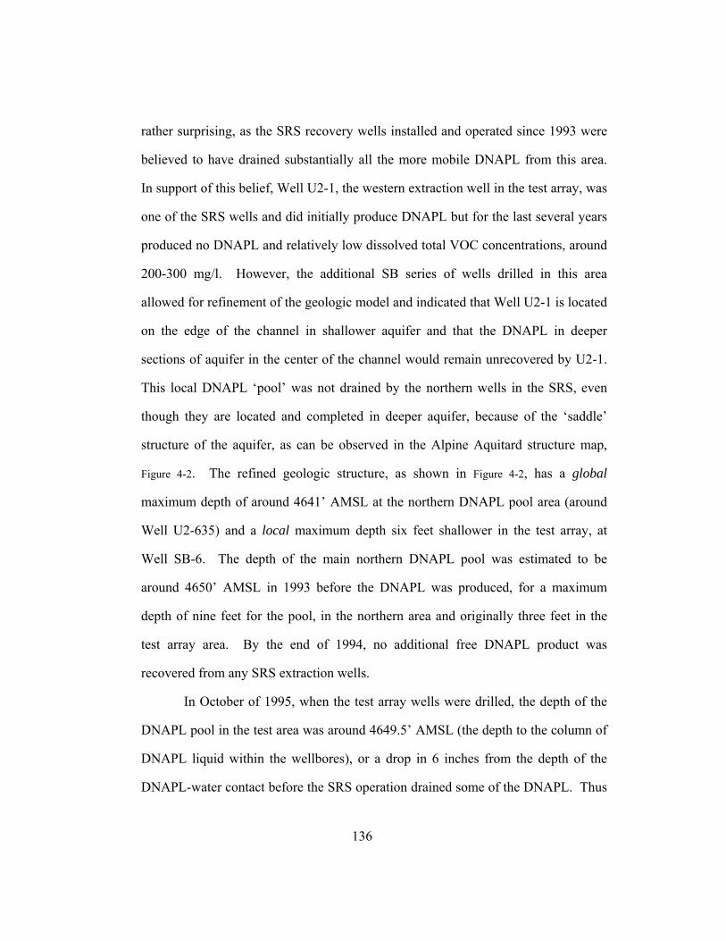
136
rather surprising, as the SRS recovery wells installed and operated since 1993 were
believed to have drained substantially all the more mobile DNAPL from this area.
In support of this belief, Well U2-1, the western extraction well in the test array, was
one of the SRS wells and did initially produce DNAPL but for the last several years
produced no DNAPL and relatively low dissolved total VOC concentrations, around
200-300 mg/l. However, the additional SB series of wells drilled in this area
allowed for refinement of the geologic model and indicated that Well U2-1 is located
on the edge of the channel in shallower aquifer and that the DNAPL in deeper
sections of aquifer in the center of the channel would remain unrecovered by U2-1.
This local DNAPL ‘pool’ was not drained by the northern wells in the SRS, even
though they are located and completed in deeper aquifer, because of the ‘saddle’
structure of the aquifer, as can be observed in the Alpine Aquitard structure map,
Figure 4-2. The refined geologic structure, as shown in Figure 4-2, has a global
maximum depth of around 4641’ AMSL at the northern DNAPL pool area (around
Well U2-635) and a local maximum depth six feet shallower in the test array, at
Well SB-6. The depth of the main northern DNAPL pool was estimated to be
around 4650’ AMSL in 1993 before the DNAPL was produced, for a maximum
depth of nine feet for the pool, in the northern area and originally three feet in the
test array area. By the end of 1994, no additional free DNAPL product was
recovered from any SRS extraction wells.
In October of 1995, when the test array wells were drilled, the depth of the
DNAPL pool in the test area was around 4649.5’ AMSL (the depth to the column of
DNAPL liquid within the wellbores), or a drop in 6 inches from the depth of the
DNAPL-water contact before the SRS operation drained some of the DNAPL. Thus

137
the DNAPL ‘pool’ thickness is around 1 foot at the extraction Well SB-1, around 2.5
feet at the monitoring Well SB-6, and around 2 feet at the injection Well SB-2 (all
before the 1995 Phase I pretest pumping). Therefore, for consistency with this
known pool of free DNAPL, the average saturations were adjusted for depths below
the 4649.5’ AMSL DNAPL contact to high values, 60% to 67% (before pre-test
DNAPL pumping), Figure 4-11. Saturations for aquifer shallower than the DNAPL
contact were then adjusted to decline gradually to zero DNAPL saturation around
5653’ AMSL, around 3.5 feet above the DNAPL contact. As shown in this figure,
this adjusted saturation distribution is consistent with depths where non-zero
DNAPL saturation was measured in the samples.
The average saturation for each of the six layers was then recalculated,
Section 2a of Table 4-6. This adjustment of the soil sample saturations for
consistency with the observed DNAPL contact increases the calculated test array
DNAPL volume from 305 gallons to 764 gallons. Subtracting the estimated 407
gallons removed from the test array during pumping would leave 357 gallons of
DNAPL within the test array at the beginning of Phase I, corresponding to an initial
DNAPL saturation of 2.4%.
A further adjustment in the saturation data was also made, for consistency
with historical DNAPL production from Well U2-1. The depth to the aquitard in the
Well U2-1 boring was around 4657’ AMSL. This was determined by gamma ray
logging conducted in 1995, as the boring log for this well was sketchy and there
were problems with the cuttings report. DNAPL was produced from Well U2-1
when it was first pumped, even though it is located about 7 feet above the estimated
4650’ AMSL DNAPL contact. For consistency with this observed U2-1 free

138
DNAPL production, the DNAPL saturations were increased slightly in the upper
regions of the aquifer around a depth of 4657’ AMSL (simulation layers 2 and 3), as
shown in Figure 4-11. One of the chemical disposal trenches is believed to have been
located in the vicinity of this well and localized high DNAPL saturations could have
existed in the U2-1 drainage area, through small stratigraphic or structural DNAPL
trapping. A stratigraphic trap could be the result of a lens of low permeability
material in the aquifer above the aquitard boundary, creating a ‘perched’ DNAPL
pool. A structural trap could be formed by a small dimple or “scour hole” structure
in the aquitard in the vicinity of U2-1.
An average adjusted DNAPL saturation distribution as a function of depth
was determined based on the soil VOC content measurements and additional data
(DNAPL pool depth and U2-1 DNAPL production). This distribution is shown as
the red-shaded line in Figure 4-11. The DNAPL volume calculated for this
distribution is shown in Table 4-6, section 3. The initial DNAPL saturation varies
from 0% near the top of the water table and increases to 67% in the deepest section
of the aquifer. The DNAPL volume is 951 gallons before pretest pumping.
Subtracting 407 gallons for the pretest pumping leaves 544 gallons at the start of
Phase I, or an initial DNAPL saturation of 3.7%.
Alternatively, Well U2-1 could have penetrated a small, high saturation
DNAPL pool, perhaps related to evidence of an old solvent barrel in the well core
borings, near the surface of the aquifer. Well U2-1 has a very long screened
interval, over 30’, and is sand-packed to within 20 feet of the ground surface, Figure
4-5: B-B’ west->east stratigraphic cross-section through Well SB-2. An extremely
localized source of DNAPL could account for the free DNAPL production in this

139
well when first produced in 1993 but might result in little DNAPL saturation
remaining within the test array. Determining the most likely scenario is difficult as
this well was not drilled recently or by current project participants and no soil
samples were analyzed and the drilling log has limited information. To make
matters even more uncertain, the amount of DNAPL production from this well is
also unknown but was apparently sufficient to cause failure of the submersible pump
parts from degradation by solvent contact and require its replacement. Inclusion of
rather ambiguous data such as the U2-1 production in developing the DNAPL
distribution for the aquifer model may have a large effect upon the chosen design,
since it increases the DNAPL volume to be remediated by 50%, from 357 to 544
gallons (Table 4-6, Sections 2b and 3b) and also changes the vertical and areal
distribution of the DNAPL. The decision is less than clear cut, but rather a question
of ‘engineering judgment’, and there are many such decisions involved in this design
process, indeed in any design. The point is not to highlight the ambiguity of the
process but rather to emphasize the need to develop ‘robustness’ in the design and to
resist ‘over-engineering’ the design, given the uncertainty in the data and in the
analyses of the data.

140
Table 4-7: DNAPL saturations calculated from contour maps, test array area
As a quality control check, this initial DNAPL volume determination was
repeated working from the contour maps directly, rather than from the aquifer
model. The aquifer model was based on the contour maps but may have
inaccuracies due to mesh discretization or human errors. The results of this quality
control check analysis are shown in Table 4-7. The aquifer pore volume for the test
array for the aquifer model is slightly larger than that for the contour map, perhaps
due to differences introduced by inclusion of the entire grid-blocks containing the
test array wells. In general, the estimates using either method agree very closely,
within 10%:
contour interval, feet AMSL: 4667 4661 4656 4655 4653 4651 4650 4649 4647 4646 4645 TOTAL
1thickness of contour interval, ft 6.5 4.5 1 2 2 1 1 2 1 1
2
area of contour interval from map, sq. ft.: 360 360 360 324 268 216 180 136 52 28 0
3 pv , cubic feet 631.8 437.4 92.34 159.8 130.7 53.46 42.66 50.76 10.8 3.78 1,6144 pv, gallons 4726.3 3272.1 690.8 1195.7 977.6 399.9 319.1 379.7 80.8 28.3 12,0705 percentage of total: 39% 27% 6% 10% 8% 3% 3% 3% 1% 0.2%
6Average Initial DNAPL Saturation: 0% 0% 0% 0% 8% 9% 5% 30% 67% 67% 2.6%
7Initial DNAPL volume: 0 0 0 0 78 36 16 114 54 19 317
8Adjusted Initial DNAPL Saturation: 0% 5% 1% 0% 10% 30% 63% 67% 67% 67% 7.6%
9Initial DNAPL volume: 0 164 7 0 98 120 201 254 54 19 917
10
Pre-test pumping DNAPL production, gallons 0 0 0 0 0 40 137 178 38 13 407
11DNAPL remaining after production 0 164 7 0 98 80 64 76 16 6 510
12DNAPL satuaration after pre-test pumping 0% 5% 1% 0% 10% 20% 20% 20% 20% 20% 4.2%
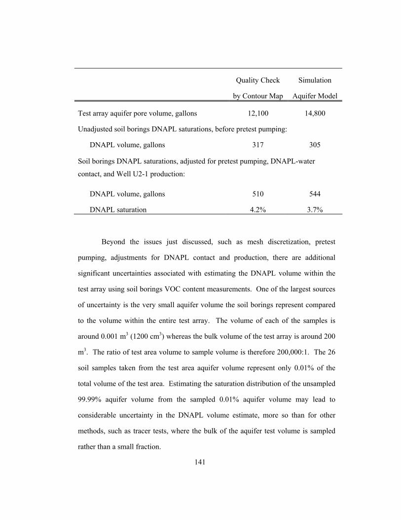
141
Quality Check
by Contour Map
Simulation
Aquifer Model
Test array aquifer pore volume, gallons 12,100 14,800
Unadjusted soil borings DNAPL saturations, before pretest pumping:
DNAPL volume, gallons 317 305
Soil borings DNAPL saturations, adjusted for pretest pumping, DNAPL-water
contact, and Well U2-1 production:
DNAPL volume, gallons 510 544
DNAPL saturation 4.2% 3.7%
Beyond the issues just discussed, such as mesh discretization, pretest
pumping, adjustments for DNAPL contact and production, there are additional
significant uncertainties associated with estimating the DNAPL volume within the
test array using soil borings VOC content measurements. One of the largest sources
of uncertainty is the very small aquifer volume the soil borings represent compared
to the volume within the entire test array. The volume of each of the samples is
around 0.001 m3 (1200 cm3) whereas the bulk volume of the test array is around 200
m3. The ratio of test area volume to sample volume is therefore 200,000:1. The 26
soil samples taken from the test area aquifer volume represent only 0.01% of the
total volume of the test area. Estimating the saturation distribution of the unsampled
99.99% aquifer volume from the sampled 0.01% aquifer volume may lead to
considerable uncertainty in the DNAPL volume estimate, more so than for other
methods, such as tracer tests, where the bulk of the aquifer test volume is sampled
rather than a small fraction.

142
Table 4-8: Uncertainties in estimating initial DNAPL volume from soil borings
Estimated Uncertainty Sources of Uncertainty
lower bound
upper bound
-? +? ± five orders of magnitude difference between small soil boring volumes (~ 0.001 m3) and the much larger total test volume (~200 m3)
-? +? ± no soil samples were available from Well U2-1, which was drilled and completed in 1993, long before the Phase I&II tests. This well is believed to have significant DNAPL in its vicinity since it produced free product initially.
0 +? +DNAPL draining from soil borings before measurement
0 +? +VOC volatilization from soil borings and cores before measurement
0 +? +non-VOC constituents in the DNAPL
-? +? ±uncertainties in equilibrium partitioning analysis method for estimating saturations from soil contaminant content, which requires assumptions regarding porosity, soil moisture content, temperature, and partitioning coefficients for each contaminant constituent.
-? +? ±uncertainties in volume of DNAPL measured from pre-test pumping
-? +? ±uncertainties in how much of volume of DNAPL measured from pre-test pumping actually within the test area
-200? +500? Estimated Total Uncertainty for Soil Borings Method, in gallons of DNAPL
Table 4-8 summarizes some of the sources of uncertainty when estimating
initial DNAPL from soil contaminant measurements. It is difficult to estimate the

143
individual uncertainties associated with each of the items listed in this table.
However, the lower and upper bounds of the total uncertainty can be very roughly
estimated by considering reasonable ranges of recoveries from primary recovery
processes. Approximately 43% of the DNAPL initially in place was recovered
during the pretest pumping, based on a value of 544 gallons of DNAPL remaining
after 407 gallons were produced. The highest reasonable recovery for a primary
recovery process would be around 60% to 70%. A 65% recovery would result in
333 gallons remaining after 618 gallons were produced. Therefore, the lower
boundary on the initial DNAPL in place estimate is around 333 gallons, or 211
gallons less than the 544 gallon value. There is considerably more uncertainty in the
upper bound estimate, especially given that the third, fourth, and fifth items on Table
4-8 could only increase the estimated DNAPL volume, but I estimate it to be around
100%, or 500 gallons.
Unfortunately, it is not possible to develop an estimate of DNAPL recovery
using soil borings data because no soil samples were obtained after the Phase II test
was completed, as the test required more time than estimated and, as always, there
were timing and budget constraints. However, even if this had been done, the
reliability of estimating remaining DNAPL from a few isolated soil borings samples
would have been problematic for the reasons discussed previously.
The development of an initial saturation distribution for the aquifer model,
and subsequent revisions as more data were obtained, is discussed further in Section
4.3.1.

144
4.2.4 LABORATORY EXPERIMENTS
The quality of the simulation predictions and the resulting field design are
directly and strongly a function of the quality and quantity of the experimental data
upon which the simulation model is based. Simulation predictions, no matter how
sophisticated and complex, with little or no experimental data to calibrate the
parametric models are likely to be very poor predictors of actual field performance.
This is particularly so for situations such as this, involving design of a field scale
surfactant remediation test, where the database of prior experience is very sparse.
The most critical types of project design information obtained from
laboratory experiments are injected chemicals selection, fluid phase behavior, and
column experiments to study the interactions between the site porous media and the
various reservoir and injected fluids.
Most of the work described in this section was conducted primarily by
Varadarajan Dwarakanath and also Douglas Shotts, building upon earlier
experimental work by Minquan Jin. A much more extensive treatment of this
material, as well as a great deal of other interesting and important work, including a
detailed laboratory protocol, may be found in Dwarakanath (1997), with additional
interesting and relevant results and analyses in Shotts (1996), Jin (1995),
Dwarakanath et al. (1999), and Dwarakanath and Pope (2000). All laboratory
results presented here not explicitly referenced are based on Varadarajan
Dwarakanath’s research, and may be found in his 1997 dissertation.

145
Phase Behavior Experiments
Extensive phase behavior experiments were conducted to select surfactants
with high contaminant solubilization, low coalescence/equilibration times, low
adsorption and minimal liquid crystal forming tendencies. Under some conditions,
surfactants may form liquid crystals and gels, usually associated with stable
macroemulsions, which may cause mass transfer limitations between trapped NAPL
and surfactant micelles and greatly impede NAPL removal efficiency (Mason and
Kueper, 1996). One very important function of laboratory experiments is to identify
these conditions. In addition, such surfactants may cause loss of hydraulic
conductivity (Renshaw et al., 1997).
The surfactants evaluated for use in this project include sodium diamyl
sulfosuccinate (commercial name Aerosol AY), sodium dihexyl sulfosuccinate
(commercial name Aerosol MA-80I), and sodium dioctyl sulfosuccinate
(commercial name Aerosol OT), all obtained from CYTEC Industries. The
cosolvents evaluated were isopropyl alcohol and secondary butyl alcohol. The
polymer evaluated was xanthan gum, a biologically generated and easily
biodegraded viscosifying agent. The electrolyte added to the surfactant solution was
sodium chloride. Additional studies were carried out using CaCl2 as an electrolyte
to determine the tolerance of the surfactant formulations to the presence of calcium
ions.
Anionic surfactants were selected because of their low adsorption on
reservoir rocks, ready availability, and low cost (Pope and Baviere, 1991; Pope and
Wade, 1995). Anionic surfactants have low adsorption because their negatively
charged hydrophilic groups are repelled by the negatively charged surfaces of clays

146
in the aquifer porous media. Surfactants with high adsorption will increase
remediation costs, as a greater mass of surfactant will be required for remediation,
and will also increase the amount of surfactant remaining in the aquifer at the end of
the test.
Dwarakanath and Pope (2000) and Jayanti (2000) evaluated surfactant phase
behavior for the remediation of field degreasing solvent DNAPLs. Mayer et al.
(1999) measured mass-transfer rates for the dissolution of TCE by surfactants and
found a near linear dependence to NAPL volumetric fraction and pore velocity.
Furthermore, the system they investigated (TCE and Aerosol MA sulfosuccinate, the
surfactant used in the field SEAR) exhibited rapid coalescence, such that equilibrium
behavior conditions apply for the expected field velocities and saturations.
Several phase behavior experiments were carried out with surfactant, alcohol
cosolvent, polymer and electrolyte mixtures. Volume fraction diagrams were
developed for various surfactant formulations by varying the electrolyte
concentrations. The DNAPL solubilization ratios of various surfactant formulations
were measured at ambient temperature (23°C) and the expected minimum aquifer
temperature of 12°C. The phase behavior data described in this dissertation and
shown in the figures may be found primarily in Dwarakanath (1997), and also Shotts
(1996), and Jin (1995).).

147
Figure 4-12: Measured organic solubility, as a function of chloride concentration, for 8 wt% MA surfactant solution, with 4% IPA, no xanthan gum, 12°C, 50% DNAPL (Dwarakanath,
1997, p. 161)

148
Sodium dihexyl sulfosuccinate (MA) was chosen as the surfactant for the
Phase I and Phase II field tests. The cosolvent chosen was 2-propanol (also referred
to as isopropanol, isopropyl alcohol, or IPA). These chemicals were selected after
many phase behavior experiments (Dwarakanath. 1997).
Figure 4-12 shows measured solubilities of the site contaminant in a solution
containing 8 % MA and 4% IPA, as a function of the concentration of sodium
chloride added to the solution. This figure illustrates the primary virtue of
surfactants for aquifer remediation: while the solubility of the Hill AFB OU2 site
contaminant in water alone is only around 1,100 mg/l, this solubility may be
increased 5400%, to 60,000 mg/l, by adding 8 wt.% surfactant to the water.
Furthermore, this solubility may be increased by another order of magnitude, to
around 625,000 mg/l, by adding 7,000 mg/l NaCl to the surfactant solution.
The microemulsion resulting from the surfactant solution coalesced in about
4 hours (Dwarakanath, et al., 1999). This is a very quick coalescence time compared
to typical residence times for the surfactant in field tests, usually of the order of 24
hours or greater. No evidence of gels or liquid crystals was observed based on
visual observations. The presence of 4 wt.% isopropyl alcohol in the injected
surfactant solution improves the performance because it increases coalescence rates
and minimizes liquid crystals and gels (Bourrel and Schechter, 1988).

149
Figure 4-12 shows a set of
measured solubilities for one
surfactant formulation, for a series
of increasing electrolyte
concentrations, sometimes referred
to as a ‘salinity scan’. Actually,
multiple series of such phase
behavior experiments were
conducted, Figure 4-13, and the
UTCHEM phase behavior model
was calibrated by evaluating the
results of these multiple phase
behavior experiments. The best
way to evaluate and compare
different phase behavior
experiments (with differing
surfactant concentrations and
optimal salinities) is to ‘normalize’
the data by plotting the solubility
ratio versus the normalized
electrolyte concentration. The
solubility ratio (the y-axis for Figure 4-13) is the concentration of contaminant in the
microemulsion divided by the concentration of surfactant in the microemulsion, with
both concentrations on a volumetric basis. The normalized electrolyte concentration
Figure 4-13: Calculated and experimental organic
solubility ratio, as a function of normalized electrolyte concentration (Dwarakanath, 1997)
0
1
2
3
4
5
6
7
8
9
0.0 0.2 0.4 0.6 0.8 1.0 1.2Normalized Electrolyte Concentration, S/S*
Sol
ubili
ty R
atio
, (C2
3/C3
3)
8% MA, 4% IPA, no xanthan, NaCl, 12°C8% MA, 8% IPA, 500 ppm xanthan, NaCl,12°C8% MA, 8% IPA, 500 ppm xanthan, NaCl, 23°C4% MA, 4% IPA, 500 ppm xanthan, NaCl, 23°C4% MA, no IPA, no xanthan, NaCl, 23°C1-8% MA, no IPA,no xanthan, no added NaCl, 23°C8% MA/4% IPA: UTCHEM Phase Behavior

150
(the x-axis for Figure 4-12) is the concentration of the electrolyte in the surfactant
solution divided by the optimal salinity. The optimal salinity, discussed in Chapter
2, is the electrolyte concentration corresponding to the lowest interfacial tensions
and is usually taken as the mid-point between the upper and lower salinities
bounding the Type III region.
Figure 4-13 shows such a ‘normalized’ plot, for several different surfactant
formulations and two different temperatures. These two temperatures correspond to
normal ambient laboratory conditions and the lowest anticipated field temperature.
The solid red line represents the UTCHEM phase behavior calibrated to Phase II
conditions and will be discussed in the next section. The surfactant formulation
shown in the previous graph (Figure 4-12) as solid black squares is also shown in this
Figure 4-13 graph as solid red squares.
The strong effect of temperature is quite apparent in this figure: The data
plotted as open and closed red squares were measured at the estimated aquifer
temperature of 12°C; all other experiments were conducted at ambient laboratory
conditions, around 23°C. For the Winsor Type I region (0.0 ≤ Cs/Cs* ≤ 0.85 to
0.95, approximately), there is a noticeable separation between measurements
conducted at the two temperatures, with the lower temperature increasing the
solubility of the contaminant in the microemulsion. The data for the two
temperatures apparently converge (within the scatter of the measurements) at higher
normalized electrolyte concentrations corresponding to Type III and Type II regions
(Cs/Cs* > 0.85 to 0.95, approximately). While an increased contaminant solubility
may seem desirable, the effect of temperature upon microemulsion phase behavior is
not an unmitigated blessing – quite the contrary, if this effect is not known, not well

151
understood, and not incorporated into the remediation design. The danger is one of
inadvertently establishing a very undesirable phase behavior region (Winsor Type II)
within the aquifer. This will be discussed further in the surfactant design section of
this chapter.
The effect of temperature is much less when no additional NaCl is added to
the surfactant solution, such as for the Phase I test conditions. There were no
changes in phase region and only a small change in measured contaminant solubility:
The GC measured solubility of the Hill contaminant in a 4 wt.% MA surfactant
solution was 15,500 mg/l at 23°C and approximately 16,000 mg/l at 12°C. The GC
measured solubility of the Hill contaminant in a 8 wt.% MA surfactant solution was
60,600 mg/l at 23°C and increased to approximately 78,000 mg/l at 12°C. (see
Figure 6.48 of Dwarakanath, 1997)
The very small effect of cosolvent can be observed in Figure 4-13 by
comparing the solid and open red squares, with IPA concentrations of 4 wt.% and 8
wt.%, respectively. Solubilities for the two different IPA concentrations virtually
overlay. (Xanthan gum is also present in one of the formulations, but this does not
alter the contaminant solubility.) A similarly small effect can also be observed by
comparing the open and closed purple diamonds, which are measured at the same
temperature and for identical surfactant formulations except for IPA concentrations,
which are 4 wt.% and 0 wt.%, respectively. Thus, cosolvent is not added to increase
solubility but rather to prevent undesirable phase behavior effects as discussed
previously. However, the presence of cosolvent does have a significant effect upon
the optimal salinity, so an ‘unnormalized’ plot would show significantly different
contaminant solubilities for a given NaCl injection concentration. For example, for a
152
8 % MA, 4% IPA formulation, at 12°C, (the solid red squares) the contaminant
solubility at 5800 mg/l added NaCl is 280,000 mg/l. Adding 4% IPA to the
surfactant solution at the same NaCl concentration would increase the contaminant
solubility by 47%, to 412,000 mg/l (the open red squares). This increase is due to
the change in phase regions: adding 4% IPA decreases the optimal salinity from
7000 mg/l to 5900 mg/l added NaCl, resulting in a Winsor Type I region for the
microemulsion with no IPA and a Type III region for the microemulsion containing
4% IPA.
The green horizontal dashes in Figure 4-13 show the low solubilization ratios
resulting from surfactant solutions without added NaCl. The solubilization ratios are
all below 1.0, ranging from around 0.2 (for 1 or 2 wt.% surfactant) up to around 0.6
(for 7 or 8 wt.% surfactant). Solubilization ratios of less than 1.0 indicate that, even
under ideal conditions, an injected gallon of 100% surfactant would recover less than
a gallon of contaminant. As actual field conditions are far from ideal, this greatly
increases the quantity of surfactant required and therefore the cost and time required
for a successful remediation. This comparison assumes that ‘solubilization’ is the
primary contaminant recovery mechanism; if mobilization is substantial, then a
surfactant formulation without added NaCl could be quite effective at recovering
substantial DNAPL, particularly if it is the more easily mobilized DNAPL present at
the beginning of a remediation project. (The issue of solubilization and/or
mobilization will be discussed later, in the test results analysis section of this
chapter.) In any case, these data highlight the desirability of adding electrolytes to
the field injection surfactant solution, even if there is regulatory resistance and
concerns about further contaminating the aquifer by injecting salt at a site already

153
massively contaminated with organic solvents. It is not even a question of choosing
the lesser evil, as the injected salt is removed from the aquifer by the many pore
volumes of water flushed through the aquifer immediately following the surfactant
injection and during the final tracer test. Of course, recovering substantially all the
injected NaCl requires that hydraulic confinement be achieved and maintained
throughout the project.

154
Figure 4-14: Comparison of experimental and calculated interfacial tension (Dwarakanath, 1997, for Hill DNAPL data)
Interfacial tensions (IFT) between water and DNAPL and between
microemulsion and DNAPL were measured and are shown by the solid markers in
Figure 4-14, plotted versus measured solubilization ratio. The interfacial tensions
measured between the DNAPL and water varied between 4-7 dynes/cm, and is
estimated to be approximately 4.8 dynes/cm. An IFT of 0.200 dynes/cm was
measured between the DNAPL and a microemulsion containing 4 wt.% sodium
0.001
0.01
0.1
1
10
0 1 2 3 4 5
Solubilization Ratio, C23/C33
Inte
rfaci
al T
ensi
on, d
yne/
cm
Hill DNAPL, distilled water, 25°C, no surf.4% MA, Hill DNAPL, 25°C, source water4% MA, Hill DNAPL, 25°C, 9000 mg/L NaCl8% MA, Hill DNAPL, 12°C, 5900 mg/l NaClAY:OT, PCE exp. data (Jin, 1995)decane exp. data (Delshad, 1986)

155
dihexyl sulfosuccinate, dissolved contaminant, no added NaCl, and Hill tap water (a
Winsor type I system, corresponds to the Phase I injection fluid). This represents a
96% reduction (over an order of magnitude difference) in IFT compared to that
between the DNAPL and groundwater alone. For a solution corresponding to the
Phase II injection fluid (4% sodium dihexyl sulfosuccinate and 11,500 mg/l added
NaCl, a Winsor type III system), the measured value was 0.097 dynes/cm. This
represents a 52% decrease in IFT measured for the Phase II surfactant solution
compared to that for Phase I.
For comparison purposes, and to illustrate the similar IFT relationships for
many disparate contaminant and surfactant systems, additional experiments are also
shown on this graph: The open squares represent IFT measurements between PCE
and a microemulsion containing 1:1 diamyl:dioctyl sulfosuccinate at 4 wt.%
concentration and added CaCl2 (Jin, 1995). The open diamonds are not even IFT
measurements for chlorinated solvents but rather for decane, a hydrocarbon
‘LNAPL’ (Delshad, 1986). These data all show a similar trend which Chun Huh
(1979) has correlated by relating the interfacial tension to the inverse of the
solubility ratio squared. This correlation has been incorporated into UTCHEM.
The viscosities of various surfactant, alcohol, polymer and electrolyte
formulations were measured before injecting them into laboratory soil column
experiments. The viscosity of the surfactant microemulsion was 1.3 cp at low shear
rates (0.1 sec-1) and changed little even at much higher shear rates (about 50 sec-1).
Adding polymer to the surfactant solution increased the viscosity to 13 cp at low
shear rates (0.1 sec-1) which decreased at higher shear rates (about 50 sec-1) to
about 7 cp. This increase in viscosities by adding polymer to the injected surfactant

156
solutions would result in improved sweep of the contaminated regions and would
reduce the number of pore volumes of surfactant required for remediation.
Development of the simulation phase behavior data from these experimental
measurements is discussed in Section 4.3.
Column Surfactant Experiments
By performing flow experiments in soil columns, DNAPL-surfactant
interactions, surfactant-field soil interactions, tracer adsorption, and surfactant
adsorption can be quantified. The optimum injection rates consistent with proper
retention times for both surfactant and tracer tests can also be determined.
Based on the phase behavior experiments discussed in the previous section
(from Dwarakanath, 1997), surfactant solution formulations were selected to
remediate DNAPL contaminated soil columns. Critical data measured included: the
amount of DNAPL recovered (and whether any DNAPL is left unrecovered),
hydraulic gradients across the soil column before, during, and after surfactant
flooding, and surfactant adsorption. Surfactants used for field applications were
selected only after satisfactory results were obtained in these soil column
experiments. It was determined that surfactants could reduce the final NAPL
saturation to less than 0.001, or around 98%-99.9% contaminant recovery, for 1.8-
2.8 pv of surfactant injected.
Three of the most important column experiments (Dwarakanath, 1997) for
the purposes of the surfactant remediation field design were:
(1) OU2#5: The column, oriented horizontally, contained DNAPL
contaminated soil samples from Well SB-6, with a permeability of 3.8 darcy and at

157
an initial saturation of around 0.13, determined by an initial tracer test, which had
low retention times (4-6 hours) which did not allow sufficient time for equilibrium
between the tracer and DNAPL to be achieved and therefore underestimated the
initial saturation. The surfactant flooding consisted of two ‘phases’: 0.5 pv of wt.%
MA in site tap water, followed by 2.7 pv of water, followed by 2.3 pv of 4 wt.%
MA, 8 wt.% IPA, 500 mg/l xanthan polymer, and 10,600 mg/l NaCl (optimal
salinity at 23°C). The column orientation was horizontal during the first phase and
vertical during the second phase. High hydraulic gradients were observed during the
second surfactant injection phase, from 0.5-0.9. The final tracer test indicated a
contaminant recovery of approximately 98.2%, with a final residual DNAPL
saturation of 0.0070.
(2) OU2#7: The column, oriented vertically, contained soil samples from
Well SB-5, with a permeability of 5.9 darcy, and was contaminated by DNAPL
flooding to an initial saturation of around 0.26, based on mass balance (Sni=0.261)
and an initial tracer test (Sni=0.255), with a residence time of 19 hours. The
surfactant flooding consisted of 2.1 pv of 4 wt.% MA, 4 wt.% IPA, 500 mg/l
xanthan polymer, and 11250 mg/l NaCl (optimal salinity at 23°C). The hydraulic
gradient was 0.23 during the initial tracer test, then peaked at 1.2 during the
surfactant/polymer flood, dropping to 0.3 during the polymer/water post-flush.
Approximately 74% of the DNAPL was produced as a ‘mobilized’ DNAPL and
26% as ‘solubilized’ dissolved contaminant. The final tracer test indicated a
contaminant recovery of approximately 99.9%, with a final residual DNAPL
saturation of 0.0002.

158
(2) OU2#8: The column, oriented vertically and maintained at 12 °C by a
water bath, contained DNAPL-contaminated soil samples from Well SB-6, with a
permeability of 7.7 darcy and at an initial saturation of around 0.08, based on an
initial tracer test, with a tracer residence time of 18 hours. The surfactant flooding
consisted of 1.8 pv of 8 wt.% MA, 8 wt.% IPA, 500 mg/l xanthan polymer, and 5850
mg/l NaCl (optimal salinity at 12 °C). The hydraulic gradient was 0.13 during the
initial tracer test, then increased to 0.25 at the start of the surfactant/polymer flood,
peaking at 0.9 at DNAPL breakthrough, dropping to 0.3 during the polymer/water
post-flush. Approximately 40% of the DNAPL was produced as a ‘mobilized’
DNAPL and 60% as ‘solubilized’ dissolved contaminant. The final tracer test
indicated a contaminant recovery of approximately 98.1%, with a final residual
DNAPL saturation of 0.0010.
The final DNAPL saturation was determined using one or more of three
independent methods:
(1) partitioning tracers: before and after surfactant flooding (only method
possible when using soil samples already contaminated with DNAPL).
(2) mass balance: by weighing the column before flooding with DNAPL
(contamination event) and after surfactant remediation.
(3) material balance: by considering the differences in the volume of
DNAPL injected during the DNAPL flood (contamination event), the
volume of DNAPL produced during the DNAPL flood, and the amount
of dissolved contaminant and DNAPL produced during the surfactant
remediation.

159
The final TCE concentration after surfactant flooding measured in the
column experiments varied from 10 mg/l down to less than the detection limit of 1
mg/l. This TCE concentration detection limit is higher than that that could be
achieved if a purge and trap mechanism were available to pre-concentrate the
samples before measurement with a gas chromatograph.
These column experiments confirmed that up to 99.9% DNAPL could be
recovered as a result of surfactant flooding, at least under ideal laboratory
conditions.
Surfactant adsorption was measured by comparing the response of a
conservative tracer (tritiated water) to that of the 14C radio-labeled sodium dihexyl
sulfosuccinate in column experiments using Hill soil. There was essentially no
retardation of the surfactant compared to the tritium tracer indicating negligible
adsorption on the soil, less than 0.3 mg/g of soil (Dwarakanath, 1997).
Column Tracer Experiments
The performance of partitioning tracers to estimate residual DNAPL
saturations was evaluated by performing several experiments. The first step was to
measure the partition coefficients of 7 partitioning tracers with site DNAPL using
static partition coefficient tests. The next step involved the use of partitioning tracers
to estimate the known residual DNAPL saturation in Ottawa sand, allowing for
determination of dynamic partitioning tracer coefficients. This was followed by
measuring tracer adsorption in uncontaminated site field soil by injecting a suite of
partitioning and non partitioning tracers into clean Hill field soil. The adsorption of
tracers by site field soil was less than 5 mg/g. This corresponded to a distribution

160
coefficient (Kd) of 0.0048 liters/kg. Dwarakanath (1997) reports that this adsorption
value was within the accuracy of the measurement and, therefore, there was
negligible adsorption of the alcohol tracers by the Hill field soil. Partitioning tracers
were used to estimate the residual saturations of contaminated field soil and
determine the minimum residence time for partitioning tracers.
Based on many laboratory experiments it was determined that a minimum
residence time of 18 hours was required to obtain accurate estimates of residual
DNAPL saturation. Tracer tests with residence times of 3.9 to 6 hours showed
distinct non-equilibrium behavior. In order to obtain accurate residual DNAPL
saturation estimates from partitioning tracer measurements, a minimum retardation
of 1.2 is recommended. In most laboratory experiments, retardation factors between
1.5 and 7 were used; however, lower retardation factors may be acceptable in field
tests, where DNAPL saturations are often lower and time and cost constraints are
greater. The average error in residual NAPL saturation estimation was 7% for the
retardation factors observed in laboratory measurements. The uncertainty in the
measurement of the retardation factors was, at most, around ± 0.035. Based on this
very conservative estimate of uncertainty, the detection limit for partitioning tracers
is a DNAPL saturation of ± 0.0004. Final NAPL saturations of less than 0.0004
(0.04% saturation) were achieved in several laboratory experiments.
The theory and applicability of partitioning tracers for estimation of DNAPL
contamination is described in detail by Jin et al. (1995), Jin (1995), and Pope et al.
(1994) and summarized in Chapter 3 of this dissertation.
Toxicity data for the tracers is summarized in the table below, as reported by
Verschueren (1983).

161
Table 4-9: Alcohol tracer toxicity
The data obtained from these laboratory experiments and used in the aquifer
tracer tests simulations included: tracer partition coefficients for the site DNAPL,
minimum residence times (or maximum rates) for tracer equilibration, tracers
suitable for this site (low loss of tracer to adsorption and volatilization, no gas
Toxicity Final Biological BiodegradationAlcohol Threshold*Extraction WeEffects ***
Concentration LD50
2-propanol 1050 mg/l ~1 mg/l 5.84 g/kg 99% removal (COD) at 52 mg/g dry inoculum/hr
1-pentanol 220 mg/l ~1 mg/l ****84% removal (BOD) after 5 days, 20°C, 333 mg/l influent.
A.S.
2-ethyl-1- butanol ** ~1 mg/l 1.85 g/kg *****
1-hexanol 62 mg/l ~1 mg/l ****57% removal (BOD) after 10 days, 20°C, 200-1,000 mg/l
influent.
1-heptanol 67 mg/l ~1 mg/l **** 28.9% removal of ThOD, A.S.
Notes:* Toxicity threshold reported is for bacteria.**No toxicity threshold was found reported.***Reported biological effects are for a single oral dose that is lethal to 50% of the rats,reported in grams of chemical admistered per kg of body weight.****No biological effect was found reported.*****No biodegradability data was found reported.

162
chromatograph interference with the site contaminants, low cost), selection of suites
of tracers with a range of partition coefficients appropriate for the range of DNAPL
saturations expected for each well pair, and tracers which exhibit no gas
chromatograph interference.
4.2.5 SURFACE TREATMENT
For the most favorable economics for the remediation, the fluids produced
during the remediation must be treatable with the existing groundwater treatment
facilities, including phase separators and a steam stripper. The high levels of
surfactant, salt, IPA, and contaminant in the recovered groundwater presented
significant challenges for steam stripper operation. Prior to the field tests, Radian
(1994b) conducted predictive modeling of the SRS surface treatment plant to
determine if and how the existing steam stripper could reduce TCE concentrations to
levels low enough to meet criteria for the municipal water treatment plant, which
treated further the water treated at the SRS. The surface treatment predictive
modeling used as input the following output from the subsurface aquifer simulation
which is the focus of this dissertation: predicted water rates, DNAPL rates, and
dissolved contaminant, surfactant, salt, and alcohol concentrations.
Additional information on this critical component of the remediation design
may be found in Oolman et al. (1995) and Radian (1994b).

163
4.3 SIMULATION MODEL DEVELOPMENT
4.3.1 AQUIFER MODEL
The aquifer model described in the following sections represents that used
for the final design cases, Cases 46 / 47 for Phase I / II. When other simulation
cases are discussed in other sections in this chapter, differences between the aquifer
models for these cases and that for Cases 46 and 47 will be summarized.
Simulation Mesh and Aquitard Structure
Choosing the mesh for a simulation is a matter of balancing the need for a
grid coarse enough for reasonably short execution times (and also time and effort
required for model development, quality control, post-processing, and analysis – all
of which are a function of the number of model gridblocks) and yet fine enough to
capture the pressure, concentration, and saturation changes between wells and within
the aquifer and the effects of aquifer heterogeneity. For these simulations, there are
six gridblocks between each of the three test array injection/extraction well pairs,
three gridblocks between each of the three injection wells, three gridblocks between
each of the three test array extraction wells, and three gridblocks between the
hydraulic control injection well and the closest test array injection well. Three
simulation layers modeled the upper 12 feet of the saturated zone and three
simulation layers modeled the lower 5.5 feet of the saturated zone, the primary area
of interest as it is believed to contain the majority of the DNAPL.

164
The aquifer model was based upon the Alpine Formation (aquitard) structure
contour map developed in Jan. 1996 by Hans Meinardus, of Intera Inc., and upon
hydraulic testing of the test array wells, also conducted and analyzed by Hans
Meinardus (discussed in Section 4.2.2). Scott Muchard, in the EWRE program at
UT, performed the very time-intensive and tedious but critically important task of
modifying the UTCHEM rock properties matrices to model the aquitard gridblocks
and thereby define the structure of the aquifer. A much preferred alternative to this
manual method would be the use of a reservoir characterization or ‘gridding’
package, such as G2/GOCAD, GRIDDER, etc. As a non-commercial, research-
oriented simulation program, UTCHEM does not currently have reservoir
characterization/gridding pre-processing packages; however, stand-alone software
programs are available, and would be essential for developing non-cartesian
coordinates and rock properties for curvilinear meshes. Alternation of the mesh
dimensions and other aquifer properties during model calibration to match historical
performance is also much facilitated by the use of such software.

165
Figure 4-15:Three-dimensional grid of site aquifer
The aquifer test volume was simulated with a three-dimensional 20 x 17 x 6
(xyz or IJL) mesh, with a total of 2040 gridblocks. Figure 4-15 shows the three-
dimensional model grid and well locations. The 3x3 line drive pattern has a line of
extraction wells (U2-1, SB-1, SB-5) to the north 10 feet apart and a line of injectors
(SB-3, SB-2, SB-4) 10 feet apart and located 18 feet south of the line of extraction
wells. A monitoring well, SB-6, is located in the center of the pattern. A hydraulic
control well, SB-8, is located 18 feet south of the line of injectors. The white
gridblocks contain aquifer; the gray contain aquitard. The section modeled in this
study is 177 feet in length from north to south, 66 feet in width from west to east,
and 19.5 feet deep from the top of the saturated zone to the deepest aquitard contour
(54 x 20 x 5.9 m). Mesh size varied from 2.5 x 2.5 x 1.5 feet (0.76 x 0.76 x 0.5 m)
0' 10' 20' 30' 40' 50' 60' 70' 80' 90' 100' 110' 120' 130' 140' 150' 160' 170'' ' '
17
1615
SB-8 SB-2SB-3
SB-5
SB-1
U2-1
Z
Y
X
1311
97
75
32
1
1
2
3456
4665
4660
4655
4650
4645
0'
10
'
20'
30'
40
'
50'
60'
66'
177'
SB-6
SB-4
1
2
3
456
19 18 17 16 14 12 10 8 6 5 4 3 2 120
N
W
E
S
19 18 17 16 14 12 10 8 6 5 4 3 2 120
FeetAMSL
L=
I= J =I=

166
for the smallest aquifer cell (19 gal or 72 l of pore volume) within the test array up to
45 x 9 x 6.5 feet (13.7 x 2.7 x 2 m) for the largest aquifer cell (5,320 gal or 20,000 l
of pore volume) at the outer, constant potential boundaries. In the test area, the three
wells in the center of the test area (extraction well SB-1, monitoring well SB-6, and
injection well SB-2) occupy the deepest portion of the aquifer, with the remaining
wells penetrating significantly thinner zones of the aquifer, since they are located on
the steeply sloping sides of the aquifer channel.
The total pore volume of the aquifer model is 217,866 gallons, with 14,807
gallons pore volume within the test array. This test array volume includes all
gridblocks within the rectangular prism bounded by, and including, the two rows of
test array wells, excluding aquitard gridblocks, for an area of 20 ft x 22.5 ft, and an
average aquifer thickness of 16 ft. A cross-section of the three-dimensional grid
passing through the three extraction wells is shown in Figure 4-16. The upper section
of this figure is a stratigraphic cross-section passing through the three extraction
wells and a delineation boring drilled to the east of the test array, showing borings
and gamma logs, and completion details for each of the extraction wells.
Sedimentology of the aquifer is indicated by pattern within the well column (see
Figure 4-3 for key), with the lightest blocks corresponding to gravels and the darkest
blocks corresponding to clay. The boundary between the clay layer and the aquifer
is indicated by the thick gray line. The central extraction well, SB-1, is drilled in the
deepest section of the aquifer. Wells U2-1 and SB-5 are higher up on the structure.
The lower section of Figure 4-16 shows the simulation grid cross-section
corresponding to this stratigraphic cross-section; the horizontal and vertical scales
for both figures are identical. The gray cells contain aquitard; the white cells are
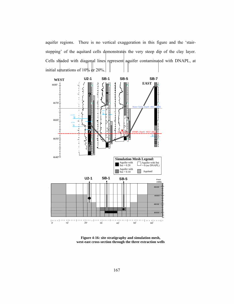
167
aquifer regions. There is no vertical exaggeration in this figure and the ‘stair-
stepping’ of the aquitard cells demonstrates the very steep dip of the clay layer.
Cells shaded with diagonal lines represent aquifer contaminated with DNAPL, at
initial saturations of 10% or 20%.
Figure 4-16: site stratigraphy and simulation mesh,
west-east cross-section through the three extraction wells
8
7
6
5
10/95
4670'
4660'
4650'
4640'
8
7
6
5
8
7
6
5
9/95
8
7
6
5
WEST
4/5/96
4/15/96
?
?
?
4 6 6 5 '
4 6 6 0 '
4 6 5 0 '
4 6 5 5 '
20'0' 60'50'40'10' 30
U2-1 SB-1
SB-5 SB-7U2-1 SB-1EAST
Simulation Mesh Legend:Aquifer with Sni= 0 (no DNAPL)
AquitardAquifer withSni = 0.10
Aquifer withSni = 0.20
SB-5
4680'
Water Table Depth: 4667' AMSL
DNAPL Depth: 4653' AMSL
WEST
Fee tA MSL
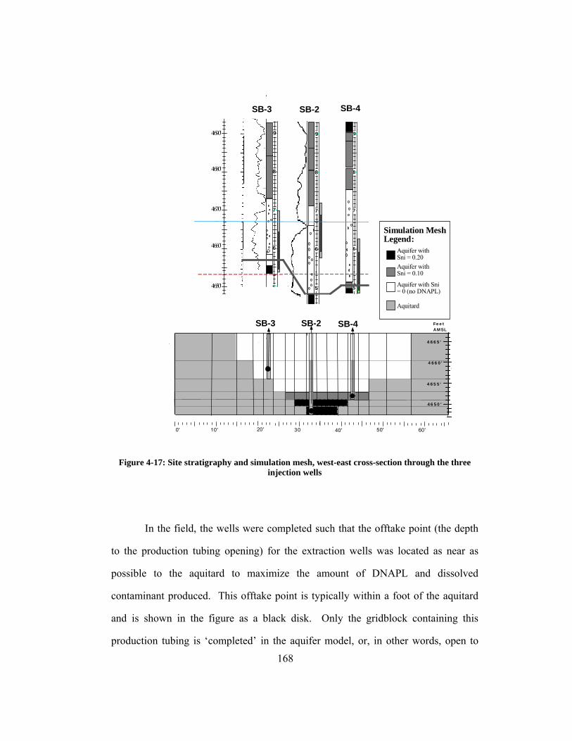
168
Figure 4-17: Site stratigraphy and simulation mesh, west-east cross-section through the three
injection wells
In the field, the wells were completed such that the offtake point (the depth
to the production tubing opening) for the extraction wells was located as near as
possible to the aquitard to maximize the amount of DNAPL and dissolved
contaminant produced. This offtake point is typically within a foot of the aquitard
and is shown in the figure as a black disk. Only the gridblock containing this
production tubing is ‘completed’ in the aquifer model, or, in other words, open to
8
7
6
5
9
44° dip
8
7
6
5
9
8
7
6
5
9
10050
4670'
4660'
4650'
4680'
4690'
4640'
SB-4SB-3 SB-2
4 6 6 5 '
4 6 6 0 '
4 6 5 0 '
4 6 5 5 '
20'0' 60'50'40'10' 30
Simulation MeshLegend:
Aquifer with Sni= 0 (no DNAPL)
Aquitard
Aquifer withSni = 0.10
Aquifer withSni = 0.20
Fe e tAMSL
SB-3 SB-2 SB-4

169
flow from the aquifer into the wellbore and then to the surface. The 12 to 15 feet
screened and sand-packed interval (the gray speckled rectangles shown in the aquifer
model cross-section and, in the stratigraphic cross-section, the gray boxes to the
right of the well sedimentology column.) of each well is modeled by increasing the
permeability (horizontal and vertical) in the gridblocks above the offtake point.
A west-east cross-section of the three-dimensional grid and the
corresponding stratigraphic cross-section passing through the three injection wells is
shown in Figure 4-17. The three injection wells are located in a slightly deeper part of
the aquifer compared to the three extraction wells. As shown in this and the
previous figure, the steeply sloping sides of the aquifer channel serve to greatly
confine the injected fluid streamlines, which can thereby only flow to the north or
south of the line of injectors.
Figure 4-18 through Figure 4-23 show the six layers of the aquifer simulation
model. Gray areas are aquitard cells. The gridblocks shaded with diagonal lines
contain initial DNAPL saturation (10% or 20%). White areas represent aquifer
uncontaminated with initial DNAPL. The north and south boundaries are open flow
and the west and east boundaries are closed by either the synclinal aquitard or the
closed model boundary. Black circles show locations of wells producing from or
injecting in this layer. Circles shaded by horizontal lines indicate wells that are
screened over the depths corresponding to this layer. Open circles show locations of
wells not producing from or injecting in this layer. There are two monitoring wells
outside the test pattern: U2-631 to the north of the test pattern, and U2-33, to the
south-east of SB-8. There are two unlabeled monitoring wells shown here, in the
I=17 row, 10 feet directly to the south of injection Wells SB-3 and SB-4. These two

170
wells do not correspond to ‘real’ monitoring wells but were included in the
simulation model to allow for monitoring of injected chemical concentrations that
tend to accumulate in the ‘stagnation zone’ that is created between the line of test
array injectors and the hydraulic injection Well SB-8.
Layers 2 through 6 are shown in Figure 4-19 through Figure 4-23, respectively.
In these figures, the very large gridblock rows on the north and south boundaries of
the aquifer (I=1 and I=20) have been truncated so that the remaining aquifer model
will be larger in the figure and details within the test array can be more readily
discerned. Flipping downward through the figures for each of the layers dramatically
shows the narrowing of the aquifer channel and the reduced area of the aquifer
within the test array. More aquitard gridblocks are required for each deeper layer.
The areal extent of the aquifer within the test array at the top of the saturated zone,
layer 1, is 360 ft2. The areal extent of the aquifer at the bottom of the channel, layer
6, 4649.5’ - 4647.5’ AMSL, is only 28 ft2, or 8% of the total test array area, with the
remaining 92% of the test array area comprised of aquitard at this depth. This very
small area is, however, very much worth modeling, as DNAPL tends to accumulate
in the deepest zones. Figure 4-23, layer 6, also shows the location of the northern
“primary pool”, (at Well U2-631 location) which in this simulation model is
modeled conceptually rather than precisely, to allow for evaluation of the effect of
surfactant in this area should significant amounts escape the test area and migrate
north upon loss of hydraulic control within the test array.

171
Figure 4-18: Layer 1 site aquifer simulation model
Legend:Aquifer Containing20% DNAPL Sat.
Aquifer Containing noDNAPL
Aquitard
Well tubing outlet in thislayer (well completed)
Well located here butscreened in otherlayer(s)
Aquifer Containing10% DNAPL Sat.
North
Layer thickness =6.5'Top of layer =4667' AMSL
Bottom of layer =4660.5' AMSL
10'
20'
30'
40'
50'
60'
80'
90'
70'
130'
100'
110'
120'
140'
150'
160'
170'
0'
177'
140'
1 7 16 15 13 11 9 8 7 6 5 4 3 2 1
XY
1
2
3
4
56789
1 01 11 21 31 41 51 6
1 7
1 8
1 9
2 0
60'50'40'30'20'10'0'
SB- 1
SB- 8
SB- 2 SB- 4SB- 3
U2 - 1
SB- 6
SB- 5
U2 -3 3
U2 -6 3 1
Well screened in thislayer
or
J =
I =
I =

172
Figure 4-19: Layer 2 site aquifer simulation model
60 '50 '40'30 '20'10 '0'
40'
50'
60'
80'
90'
70'
130'
100'
110'
120'
140'
150'
140'
17 16 15 13 11 9 8 7 6 5 4 3 2 1
2
3
4
56789
1 01 11 21 31 41 51 6
1 7
1 8
1 9
SB- 1
SB- 8
SB- 2 SB- 4SB- 3
U2 - 1
SB- 6
SB- 5
U2 - 3 3
U2 - 6 3 1
Layer thickness = 4.5'Top of layer = 4660.5' AMSLBottom of layer = 4656' AMSL
Nort h
I =
J =

173
Figure 4-20: Layer 3 site aquifer simulation model
6 0 ' 5 0 ' 4 0 ' 3 0 ' 2 0 ' 1 0 ' 0 '
40'
50'
60'
8 0 '
9 0 '
7 0 '
1 3 0 '
1 0 0 '
1 1 0 '
1 2 0 '
1 4 0 '
1 5 0 '
1 4 0 '
1 7 1 6 1 5 1 3 1 1 9 8 7 6 5 4 3 2 1
2
3
4
5 6 7 8 9
1 0 1 1 1 2 1 3 1 4 1 5 1 6
1 7
1 8
1 9
S B - 1
S B - 8
S B - 2 S B - 4 S B - 3
U 2 - 1
S B - 6
S B - 5
U 2 - 3 3
U 2 - 6 3 1
Layer thickness = 3'Top of layer = 4656' AMSL Bottom of layer = 4653' AMSL
N o r t h
I =
J =

174
Figure 4-21: Layer 4 site aquifer simulation model
6 0 ' 5 0 ' 4 0 ' 3 0 ' 2 0 ' 1 0 ' 0 '
40'
50'
60'
8 0 '
9 0 '
7 0 '
1 3 0 '
1 0 0 '
1 1 0 '
1 2 0 '
1 4 0 '
1 5 0 '
1 4 0 '
1 7 1 6 1 5 1 4 1 2 1 0 9 8 7 6 5 4 3 2 1
2
3
4
5 6 7 8 9
1 0 1 1 1 2 1 3 1 4 1 5 1 6
1 7
1 8
1 9
S B - 1
S B - 8
S B - 2 S B - 4 S B - 3
U 2 - 1
S B - 6
S B - 5
U 2 - 3 3
U 2 - 6 3 1
Layer thickness = 2'Top of layer = 4653' AMSL Bottom of layer = 4651' AMSL
N o r t h
I =
J =

175
Figure 4-22: Layer 5 site aquifer simulation model
6 0 ' 5 0 ' 4 0 ' 3 0 ' 2 0 ' 1 0 ' 0 '
40'
50'
60'
8 0 '
9 0 '
7 0 '
1 3 0 '
1 0 0 '
1 1 0 '
1 2 0 '
1 4 0 '
1 5 0 '
1 4 0 '
1 7 1 6 1 5 1 4 1 2 1 0 9 8 7 6 5 4 3 2 1
2
3
4
5 6 7 8 9
1 0 1 1 1 2 1 3 1 4 1 5 1 6
1 7
1 8
1 9
S B - 1
S B - 8
S B - 2 S B - 4 S B - 3
U 2 - 1
S B - 6
S B - 5
U 2 - 3 3
U 2 - 6 3 1
Layer thickness = 1.5'Top of layer = 4651' AMSL Bottom of layer = 4649.5' AMSL
N o r t h
I =
J =

176
Figure 4-23: Layer 6 site aquifer simulation model
6 0 ' 5 0 ' 4 0 ' 3 0 ' 2 0 ' 1 0 ' 0 '
40'
50'
60'
8 0 '
9 0 '
7 0 '
1 3 0 '
1 0 0 '
1 1 0 '
1 2 0 '
1 4 0 '
1 5 0 '
1 4 0 '
2
3
4
5 6 7 8 9
1 0 1 1 1 2 1 3 1 4 1 5 1 6
1 7
1 8
1 9
S B - 1
S B - 8
S B - 2 S B - 4 S B - 3
U 2 - 1
S B - 6
S B - 5
U 2 - 3 3
U 2 - 6 3 1
Layer thickness = 2'Top of layer = 4649.5' AMSL Bottom of layer = 4647.5' AMSL
N o r t h
1 7 1 6 1 5 1 4 1 2 1 0 9 8 7 6 5 4 3 2 1
I =
J =

177
Figure 4-24 shows the three south to north cross-sections passing through the
three extraction/injection well pairs. Screened intervals are indicated by solid black
rectangles. The well completion (well tubing opening) is located in the deepest
gridblock of the screened interval. These cross-sections illustrate the much lower
degree of relief along the axis of the channel compared to cross-sections
perpendicular to the axis channels, Figure 4-16 and Figure 4-17.
Figure 4-24: Hill AFB OU2 aquifer model simulation mesh, north-south cross-sections through each of the three injection/extraction test array well pairs
.
19 18 17 16 14 12 10 9 8 7 6 5 4 3 2 120
SB-5SB-4S N
0' 20' 30' 40' 60' 70' 80' 90' 100' 110' 120' 130' 140' 150' 160' 170' 177'50' 10'
A M S L 4670'
4660'
4650'
19 18 17 16 14 12 10 9 8 7 6 5 4 3 2 120
SB-8SB-2
SB-6SB-1
S N A M S L 4670'
4660'
4650'
19 18 17 16 14 12 10 9 8 7 6 5 4 3 2 120
A M S L 4670'
4660'
4650'
SB-3 U2-1 U2-631 N S
A q u i f e r w i t h S n i = 0 ( n o D N A P L ) A q u i t a r d
A q u i f e r w i t h S n i = 0 . 1 0
A q u i f e r w i t h S n i = 0 . 2 0
S i m u l a t i o n M e s h L e g e n d :
I=
I=
I=
I=
I=
I=
J = 13 cross-section:
J = 9 cross-section:
J = 5 cross-section:

178
Model boundaries and hydraulic gradient
The site natural hydraulic gradient is approximately 0.002 (Intera, 1997), or
around two orders of magnitude less than the 0.10 to 0.20 artificial gradients induced
during the field tests and was, therefore, neglected in the design simulations. Open
boundaries were placed at the north and south sections of aquifer model to allow
flow into and out of the aquifer in response to the test area injection and extraction.
These boundaries are located 80 feet (24 m) from the test array borders. Both north
and south boundaries maintain a constant potential equal to the hydrostatic head.
The western and eastern model boundaries are closed boundaries
approximately 23 feet (7 m) from the test array borders and these edges are primarily
aquitard gridblocks. The lower boundary of the aquifer is also comprised primarily
of aquitard cells, with the lower boundary of the aquifer model a closed boundary.
The upper boundary of the aquifer model is modeled as a closed boundary as
well and is initialized at atmospheric pressure depth with the pressure increasing by
the hydrostatic head downwards. The upper boundary is fixed; in other words, the
water table depth is assumed to be flat and at a constant depth throughout the test.
Sensitivity tests with and without the vadose zone were conducted in initial
scoping work. Remediation performance (measured by extraction well produced
concentrations and aquifer DNAPL saturations with time) was not sensitive to
including the vadose zone. Therefore, the vadose zone was not included in the
design and post-test simulation models. This allowed grid blocks to be concentrated
where most needed, in the lower aquifer DNAPL zone, while still keeping CPU time
reasonable.

179
Aquifer permeability and porosity
The degree of variability of the permeability within the aquifer is an
unknown. Firstly, there were very few permeability measurements taken. Secondly,
determining realistic in situ properties for these unconsolidated samples can be very
difficult, due to rearrangement of the grains and disruption of the porous media
during boring, transport, cutting, and storage. This disruption is exacerbated by the
many large cobbles in the gravel comprising the aquifer. Measured soil borings
samples permeability ranged from 3.9 to 44 darcy (Oolman et al., 1995, and
Dwarakanath, 1996). Hydraulic conductivities determined from the hydraulic tests
ranged from 1 to 14 x10-5 m/s (equivalent to a permeability of 1 to 14 darcy). These
permeabilities cannot be used directly in estimating small scale variations, as they
represent average hydraulic conductivity over a well’s entire drainage volume, a
volume much larger than the aquifer model’s 2.5 x 2.5 x 1.5 feet gridblock size.
Also, some of the variation may have been due to lower hydraulic conductivity for
some wells from the presence of DNAPL interfering with water flow within the
pores. As a matter of fact, the lowest conductivity from the hydraulic testing was
measured for Well SB-6, which was also the deepest well in the test array and,
therefore, likely to have the greatest quantity of DNAPL in the well drainage
volume.
For the simulation cases presented here, a three-dimensional stochastically
generated permeability field with a mean of 20 darcy (20 µm2) was used. The mean
permeability is equivalent to a hydraulic conductivity of 55 ft/day or 20x10-5 m/s, for
a porous media saturated with water only, at normal density and viscosity. The
correlation lengths for the stochastic permeability field were chosen based upon
180
depositional environment (lenticular accumulations) and a qualitative evaluation of
the well logs in the test area, which indicated little correlation in sedimentology even
for wells as close as 10 feet (3 meters). A value of 5 feet (1.5 m) was chosen for the
y direction correlation length, perpendicular to the aquifer channel axis, and a
correlation length of 10 feet (3 m) was chosen for the x direction, parallel to the
aquifer channel axis. The correlation length in the vertical direction was set to 1 foot
(0.3 m), resulting in no vertical correlation in the permeability fields generated for
these simulations, where the vertical mesh was at least 1.5 feet (0.5 m).
The degree of permeability variation for the aquifer model was selected by
the following method: Three different stochastic permeability fields were generated
and evaluated:
(1) SD ln k = 0.92, VDP=0.60,
(2) SD ln k = 1.2, VDP=0.70, and
(3) SD ln k = 1.6, VDP=0.80,
where ‘SD ln k’ is the standard deviation in the natural log of the
permeabilities and VDP is the Dykstra Parsons coefficient for variation in
permeability (Dykstra and Parsons, 1950), commonly used for petroleum reservoirs.
Table 4-10 summarizes the permeability and its variation, by layer, for each of the
three realizations. For the realization with the lowest permeability variation (SD ln k
= 0.92, VDP=0.60), only 0.3% of the gridblocks have permeabilities less than 1 darcy
(1 µm2) and 0.8% have permeabilities greater than 100 darcy (100 µm2). For the
realization with the mid-level of variation (SD ln k = 1.2, VDP=0.70), 4% of the
gridblocks have permeabilities less than 1 darcy and 2% have permeabilities greater
than 100 darcy. For the realization with the highest degree of permeability variation,

181
(SD ln k = 1.6, VDP=0.80), 14% of the gridblocks have permeabilities less than 1
darcy and around 3% have permeabilities greater than 100 darcy. The three different
stochastic permeability fields were compared and a standard deviation in ln k of 1.2
(VDP=0.70) was chosen as being most consistent with: (1) typical variations
observed in other porous media and (2) the range of permeabilities for the Hill OU2
measured permeabilities.

182
Table 4-10: Summary of three stochastic permeability fields, at 0.6, 0.7, and 0.8 Dykstra-Parsons Coefficients
For the chosen stochastic permeability field used in the final remediation
design simulations, the permeability in the aquifer is a mean 20 darcy (20 µm2), with
For Vdp = 0.60 Realization:overall Layer 1 Layer 2 Layer 3 Layer 4 Layer 5 Layer 6
mean 19,760 22,510 15,510 15,320 14,840 21,290 29,120 SD 21,100 25,460 11,700 17,510 15,130 20,980 27,540
SD lnK 0.92 0.88 0.81 0.95 0.88 0.95 0.80CV 1.07 1.13 0.75 1.14 1.11 0.99 0.95Vdp 0.60 0.59 0.55 0.61 0.58 0.61 0.55min K 601max K 230,000 # cells < 1 Darcy 6 0.3%# cells > 100 Darcy 16 0.8%
For Vdp = 0.70 Realization:overall Layer 1 Layer 2 Layer 3 Layer 4 Layer 5 Layer 6
mean 19,460 23,360 13,290 14,070 12,280 21,280 31,510 SD 30,580 38,660 13,760 25,330 19,000 28,520 43,090
SD lnK 1.20 1.16 1.06 1.24 1.15 1.25 1.05CV 1.57 1.66 1.04 1.80 1.43 1.34 1.37Vdp 0.70 0.49 0.65 0.71 0.68 0.71 0.65min K 168max K 417,000 # cells < 1 Darcy 78 3.8%# cells > 100 Darcy 49 2.4%
For Vdp = 0.80 Realization:overall Layer 1 Layer 2 Layer 3 Layer 4 Layer 5 Layer 6
mean 18,700 24,510 9,933 12,460 10,990 20,340 33,950 SD 47,040 60,910 15,320 40,980 23,150 38,770 72,110
SD lnK 1.61 1.55 1.42 1.66 1.54 1.67 1.41CV 2.52 2.49 1.54 3.29 2.11 1.91 2.12Vdp 0.80 0.79 0.76 0.81 0.79 0.81 0.76min K 24max K 836,000 # cells < 1 Darcy 290 14.2%# cells > 100 Darcy 57 2.8%

183
a 1.44 variance in ln k (equivalent to a 0.70 Dykstra Parsons coefficient) and a range
in permeability from 0.2 to 417 darcy (0.2 µm2 to 420 µm2), or a range of over three
orders of magnitude. The stochastic permeability field is illustrated in Figure 4-25, a
three-dimensional grid, and in Figure 4-26, showing the distribution for each of the
six model layers. The aquitard boundary is shown by the heavy black boundary
between the constant permeability aquitard cells and the variable permeability
aquifer cells. Due to limitations in the graphics software (Spyglass), the variation in
the mesh size, shown in previous figures, cannot be represented here. This figure
and all subsequent concentration and saturation maps will likewise not be to scale
and model boundaries will appear nearer the test array than they actually are.
However, the test array and the immediately adjacent gridblocks all have the same
mesh (2.5 x 2.5 feet) so there is no distortion in these and subsequent maps in the
immediate test array area.

184
Figure 4-25: Aquifer Model Permeability, 3D view
Aquifer Permeability, in Darcy
U2-1
SB-1
SB-5
SB-3
SB-2
hill 45permxEAST
WEST
20 15 10 5 0
SB-4
SB-6
SB-8

185
Figure 4-26: Site Aquifer Model Permeability, by layer
The aquifer porosity throughout the model was set to a constant 27%. This
is based on the average for porosities measured in borings from the OU2 site, which
ranged from 22.2% to 32.1% (TerraTek, 1994).
Layer 1 Layer 2 Layer 3
Horizontal Permeability, in Darcy
Layer 4 Layer 5 Layer 6
8 7 6 5 4 3 2 1 0
NE
SW

186
This porosity was increased from 27% to 90% in the few gridblocks on the
east and west boundaries of the model (columns J=1 and J=17, see Figure 4-15).
This allowed the pore volume of the aquifer channel in this area distant from the test
array to be modeled accurately while minimizing the total number of model
gridblocks.
Aquitard permeability and porosity
The steeply dipping lower boundary of the aquifer was modeled by assigning
lower permeability and porosity to all gridblocks lying within the aquitard.
The hydraulic conductivity of samples from the clay aquitard borings from
the site was measured as 9.6 x 10⁻¹¹ m/s or 2.7 x 10⁻⁵ ft/yr, equivalent to a
permeability of 1 x 10⁻⁵ darcy or 0.01 md (Core Laboratories, 1996; Intera, 1996).
This is an extremely low hydraulic conductivity. The measured permeability was
adjusted to 0.005 md for input into UTCHEM to result in the appropriate
transmissibility across the aquitard boundary, because UTCHEM includes
permeability of both upstream and downstream gridblocks in calculating the
transmissibility. The vertical permeability was set equal to 1/10 the horizontal
permeability over the entire aquifer model, for both aquifer and aquitard gridblocks.
The porosity of the aquitard was set to a low value, 1%. This does not
represent the actual measured porosity of the clay but was chosen rather to minimize
the pore volume in the aquitard and, therefore, minimize anomalous material balance
results and spurious simulation graphics resulting from numerical dispersion and
other effects into the gridblocks containing clay. In any case, the primary focus here

187
is the behavior of the aquifer and aquitard gridblocks are included primarily to
define topography.
An alternative to modeling the aquitard as low permeability gridblocks
would be the use of curvilinear coordinates to specify a complex lower aquifer
boundary, thereby excluding the aquitard entirely. This alternative was not chosen
for the aquifer model because of time and code constraints. At the time these
simulation studies were conducted, the curvilinear option for UTCHEM was not yet
extensively tested and curvilinear variation was possible only in two dimensions,
whereas the complex shape of the site aquitard required variation in all three
dimensions.
Initial DNAPL distribution
For the Phase I design simulations, such as Case 17, published in the Phase I
Work Plan submitted by Intera to the Air Force (before the test was conducted), and
preliminary Phase II design simulations, the DNAPL saturation was set to 0.20 in the
lowest three simulation layers (excluding aquitard regions), representing the lowest
5.5 feet (2 m) of the aquifer. The upper 14 feet (4.3 m) of the aquifer (the upper
three model layers) contained no DNAPL in the test area. The initial saturation at
the beginning of Phase I in the model aquifer within the test array was approximately
4%, by the volumetric average of the initial saturations (either 20% or 0%).
For the final Phase II design simulations and Phase I simulations conducted
after the Phase I field test, such as Phase I Case 46 and Phase II Case 47, the initial
DNAPL saturation distribution is consistent with that described in the text and table
in Section 4.2. The lowest 3.5 feet (1.1 m, simulation layers 5-6) of the aquifer was

188
set to an initial DNAPL saturation of 20% and the next higher 2 feet (0.6 m,
simulation layer 4) was set to 10%. The upper 14 feet (4.3 m, simulation layers 1-3)
contained no DNAPL except for a small volume around the U2-1 well completion
with an initial DNAPL saturation of 20%. When the initial saturations throughout
the test area (either 20%, 10%, or 0%) are volumetrically averaged, the average
initial saturation in the model test area is approximately 4%. The Phase II
simulations were executed as a continuation or ‘restart’ of the Phase I simulations;
therefore, the DNAPL distribution at the beginning of the Phase II simulation was a
heterogeneous distribution and a function of the predicted Phase I test performance.
Figure 4-27 is a three-dimensional representation of initial DNAPL distribution. The
initial DNAPL saturation for each of the six model layers is shown in Figure 4-28.
These figures show the initial DNAPL saturation at the beginning of the Phase I test
simulation. The slight amount of DNAPL saturation lost by dissolution during the
three day injection/extraction period before the Phase I test began is apparent in the
last figure, particularly around the injection and extraction well completions in layers
4-6.

189
Figure 4-27: Site aquifer model 3-D DNAPL distribution at the beginning of Phase I Pilot Test
DNAPL Saturation, vol./vol.
Light blue shaded area envelopes all DNAPL saturations greater than 0.006. Transparent areas of mesh represent aquifer with DNAPL saturations lower than 0.006.
Note:
0.00 0.05 0.10 0.15 0.20 0.25
hill 46a. s2.t01
U2-1
SB-1
SB-5
SB-3
SB-2
SB-4
EAST

190
Figure 4-28: Site aquifer model distribution at the beginning of Phase I Pilot Test, by layer.
The DNAPL saturation distribution at the beginning of the Phase I test
encountered in the actual field test is certainly more complex than this assumption of
either 20%, 10%, or 0% DNAPL saturation for the Phase I simulations. A
heterogeneous initial DNAPL saturation could have been developed for the model
by simulating and history-matching the pre-test DNAPL pumping, but I chose to use
Layer 1 Layer 2 Layer 3
Nxxxxxxxxx hill46a. c2. t01hill46a.c2.t01hill 46a.c2.t01
Contaminant Saturation, vol./vol.
0.00 0.05 0.10 0.15 0.20 0.25
Layer 4 Layer 5 Layer 6
N
E
S
W
hill 46a.c2.t01 hill 46a.c2.t01 hill 46a.c2.t01

191
a simpler DNAPL saturation distribution both because of time limitations and
because there was much uncertainty in critical data needed for model history-
matching such as pumping rates and timing, pre-test DNAPL saturation distribution,
capillary pressure, relative permeability, and the permeability distribution throughout
the aquifer. This uncertainty decreases the value of such history-matching by
decreasing the probability that the history-matched aquifer model represents actual
aquifer conditions, the ‘non-uniqueness’ problem. An even more ambitious
approach would have been to model the contamination event itself as well, but this
approach is fraught with even more uncertainties and unknowns, including but not
limited to the surface locations and geometry of the original disposal trenches (which
have since been buried), the volume and composition of DNAPL deposited, and the
times and rates for the DNAPL contamination events.
University of Texas graduate students working with Dr. Daene C. McKinney
and Dr. Gary A. Pope researched the use of inverse modeling of tracer tests to better
estimate this initial DNAPL distribution, as well as permeability distribution. Such
an approach would be extremely valuable as a tool for better understanding of the
results of the field tracer and remediation tests. It would be even more valuable as a
design tool, to improve the site characterization and aquifer model, if sufficient time
(and manpower) could be allowed between the partitioning tracer tests and the
surfactant injection.
In all simulations the northern “primary” pool (in the U2-631 area) was
included but modeled only conceptually, with a small number of cells, so that the
effect of any surfactant escaping the test area and entering the northern pool area
could be discerned. The initial DNAPL saturation of all grid blocks within this

192
northern pool was set to 20%. The only change in DNAPL saturations observed in
this northern pool area was a small decrease caused by dissolution of the DNAPL
into groundwater flowing toward the test area, a function of the overproduction
design conditions.
4.3.2 PHASE BEHAVIOR
Phase Regions and Contaminant Solubility
In UTCHEM, phase behavior parameters define the solubility of the organic
in the microemulsion, as a function of surfactant and electrolyte concentrations. In
Section 2.3, UTCHEM’s phase behavior model is summarized. Section 4.2.4
summarizes results of a series of phase behavior experiments, which determined
contaminant solubility at two different temperatures, and various anion, surfactant,
and cosolvent concentrations. Figure 4-13 shows the experimental solubility ratio
(33
23
CC
) versus the normalized electrolyte concentration (s
s
CC
* ) for a series of
experiments and also shows the UTCHEM predicted phase behavior used for the
Phase II simulations. The primary phase behavior parameters adjusted were C3max0
and C3max1, the maximum surfactant concentrations at zero and optimal salinity,
respectively, C3max is also the height of the binodal curve bounding the single phase
region on a ternary phase diagram.

193
Figure 4-29: Phase Behavior Schematic, for 8 wt.% MA, 4 wt.% IPA, 7000 mg/l added NaCl, at
12 oC.
Figure 4-12 shows this same UTCHEM predicted phase behavior and
experimental data, for the 8% MA, 4% IPA, 12°C experiment, in a slightly different
and perhaps more conventional form: as solubility in mg/l versus added NaCl
concentration. An additional adjustment was made in the experimental data shown
in this figure: the solubilities were adjusted from Winsor Type III to Winsor Type II.
The adjustment occurs over a very narrow range of data and, for the 8% MA / 4%
IPA / 12°C experiment, involved only one point.
Three major simplifications were made in the simulation of the
experimentally observed phase behavior:
volume of DNAPL entering themicroemulsion
U = 0 . 9 4 m l
I n i t i a l c o n d i t i o n s , b e f o r e m i x i n g :
injected surf. solution:8 wt.% MA surfactant, 4 wt.% IPA cosolvent, 7000 mg/l added NaCl, in site tap water, 12ÁC
s i t e D N A P L
V i n j = 2 . 0 6 m l
I F i = 3 . 0 m l
L = 5 . 0 m l
V o = 2 . 0 m l
A f t e r m i x i n g a n d e q u i l i b r a t i o n :
I F m o = 3 . 9 2 m l
excess aqueousphase:tap water and added NaCl
e x c e s s o l e i c p h a s e : s i t e D N A P L
volume of inj.surf. solutionentering themicroemulsion
I F w m = 1 . 8 8 m l
V o = 1 . 0 8 m l
U = 0 . 9 4 m l
L = 5 . 0 m l
V m = 2 . 0 4 m l
V w = 0 . 9 4 m l
m i d d l e p h a s e m i c r o e m u l s i o n : c o n t a m i n a n t , M A s u r f a c t a n t , I P A c o s o l v e n t , a d d e d N a C l , t a p w a t e r

194
• The narrow phase region between the lower effective salinity and the
optimal salinity was modeled as a Winsor Type I rather than a Type III
system and is discussed later in this section. This simplification was
needed only for the Phase II design simulations, as Phase I did not have
additional electrolytes (NaCl) injected and was a Type I system
throughout the Phase I test.
• Since the site contaminant is composed primarily of TCE, the
contaminant was modeled as a single oleic component, with properties
corresponding to those measured for the site DNAPL, which consisted of
around 73% TCE, 14% 1,1,-TCA, and 8% PCE. Current versions of
UTCHEM have the capability of modeling multiple oleic components, if
this additional simulation complexity is justified by the site contaminant
characteristics, such as high concentrations of several components,
particularly if the properties of these components are quite disparate.
• The IPA cosolvent was not modeled explicitly as a separate component.
Instead, it was ‘lumped’ with the surfactant component to form a
‘pseudo’ surfactant component. This is similar to the ‘lumping’ involved
in the modeling of the contaminant component. The phase behavior
parameters were adjusted so that the five components in UTCHEM (C1 =
water; C2 = contaminant; C3 = surfactant + IPA; C5 = anion) matched
the phase behavior for the actual experimental system, which consisted
of multiple cation, anion, and DNAPL components, as well as the
alcohol. The surfactant density was adjusted to include the effect of the

195
lighter IPA cosolvent so that the proper mixture density was calculated in
UTCHEM.
Figure 4-29 is a schematic showing a typical phase behavior experiment, for
a pipette containing DNAPL and an injection solution containing 8 wt.% sodium
dihexyl sulfosuccinate (MA), 4 wt.% 2-propanol (IPA), and 7000 mg/l NaCl added
to the Hill site tap water. Equal volumes of this injection solution and the OU2 site
contaminant were mixed in a pipette which was sealed and allowed to equilibrate.
The pipette was maintained at 12°C by a cold water bath. The electrolyte
concentration, 7000 mg/l added NaCl, is the approximate optimal salinity, where the
components coalesce into three phases. The volume of each phase is obtained by
subtracting the interface levels (IF), as shown in Figure 4-29. The volumetric
quantity of NAPL, surfactant, IPA, and water in the microemulsion phase may be
found by:
ml92.00.392.3 =−=−= imoom IFIFV (4.3-1)
( ) ml13.0=ml25.1005.116.006.208.0 ⎟
⎠⎞
⎜⎝⎛===
s
injsism VV
ρρ
(4.3-2)
( ) ml10.0=ml786.0005.108.006.204.0 ⎟
⎠⎞
⎜⎝⎛===
a
injaiam VV
ρρ
(4.3-3)
ml89.010.013.092.004.2 =−−−=−−−= amsmommwm VVVVV (4.3-4)
Likewise, the volumetric concentration of contaminant, surfactant, alcohol,
and water within the microemulsion phase may be found by:
45.004.292.0
23 ===m
om
VV
C (4.3-5)

196
064.004.213.0
33 ===m
sm
VV
C (4.3-6)
049.004.210.0
3 ===m
ama V
VC (4.3-7)
44.004.289.0
13 ===m
wm
VV
C (4.3-8)
The sum of the component concentrations equals 1.003 (not exactly 1.0 due
to rounding). The cation and anion concentrations are not included in this sum, as
they are assumed to occupy negligible volume within the microemulsion. For this
Winsor Type III system, the water solubilization parameter is:
72.6064.044.0
33
13 ==CC
(4.3-9)
The oil solubilization parameter is:
03.7064.045.0
33
23 ==CC
(4.3-10)
The oil solubilization parameter may be easily converted to contaminant
solubility in the microemulsion, in units of mg/l:
( ) ( )l
mggmg
literml
mlg
mlmlC o 000,620
11000
1100038.145.023 === ρ (4.3-11)
These calculations, Eqs. 4.3-1 through 4.3-11, include the following
assumptions:
(1) There is no change in volume after mixing (ideal mixing).

197
(2) The amount of contaminant dissolved in the excess water phase may
be neglected.
(3) All of the surfactant and alcohol remains within the microemulsion
phase; i.e., surfactant and alcohol concentrations within the excess water and oleic
phases are negligible.
To confirm that these assumptions were reasonable and appropriate, the total
fluid volume before and after mixing was observed to remain constant and the
concentrations of individual components were measured with a gas chromatograph.
If any of these assumptions are not appropriate for a different set of site and injected
fluids, then the preceding calculations should be modified accordingly.
In the Phase II simulations, the Winsor Type III behavior was modeled as a
Winsor Type I system, to simplify the required analyses and code modifications. In
other words, two phases, the excess aqueous phase and the middle phase
microemulsion, were modeled as an aqueous phase microemulsion. In this example,
Figure 4-29, the 0.94 ml of excess aqueous phase, 2.04 ml of microemulsion, and
1.08 ml of DNAPL would be modeled as 2.98 ml of microemulsion and 1.08 ml of
DNAPL. This simplification had no effect upon the calculated volumetric quantities
of NAPL, surfactant, IPA in the microemulsion phase:
ml92.00.392.3 =−=−= imoom IFIFV (4.3-12)
( ) ml13.0=ml25.1005.116.006.208.0 ⎟
⎠⎞
⎜⎝⎛===
s
injsism VV
ρρ
(4.3-13)
( ) ml10.0=ml786.0005.108.006.204.0 ⎟
⎠⎞
⎜⎝⎛===
a
injaiam VV
ρρ
(4.3-14)

198
compared with Eqs. 4.3-1 through 4.3-3, but almost doubled the volume of
water in the microemulsion phase:
ml83.110.013.092.098.2 =−−−=−−−= amsmommwm VVVVV (4.3-15)
compared with Eqs. 4.3-4. The volumetric concentrations of NAPL,
surfactant, and alcohol within the microemulsion phase for the modeled Winsor
Type I system decreased slightly and the water concentration increased compared to
Eqs. 4.3-5 to 4.3-8:
31.098.292.0
23 ===m
om
VV
C (4.3-16)
044.098.213.0
33 ===m
sm
VV
C (4.3-17)
034.098.210.0
3 ===m
ama V
VC (4.3-18)
61.098.283.1
13 ===m
wm
VV
C (4.3-19)
However, and most importantly, the oil solubilization parameter is identical
for this simplified Winsor Type I system compared to that for the Winsor Type III
(Eq. 4.3-10):
05.7044.031.0
33
23 ==CC
(4.3-20)
In other words, even though individual component concentrations vary
slightly for the simplified system (Winsor Type I) compared to the original Winsor
Type II system, the dissolving capacity of the surfactant, as measured by the oil
solubilization parameter, remains the same. However, the contaminant solubility in

199
units of mg/l is lower because, even though the mass of contaminant dissolved
remains the same, the volume of microemulsion is larger. The contaminant
solubility in the microemulsion, in units of mg/l is:
( ) ( )l
mggmg
literml
mlg
mlmlC o 000,430
11000
1100038.131.023 === ρ (4.3-21)
compared to 620,000 mg/l calculated in Eq. 4.3-11.
To model the Winsor Type III behavior at 7000 mg/l added NaCl as a
Winsor Type I system, selC , the lower salinity defining the transition between Type
I and Type III must be increased in the UTCHEM simulations from the experimental
value of approximately 6500 mg/l to a value greater than 7000 mg/l added NaCl.
This selC value was adjusted further to provide an additional tuning parameter to
better match measured contaminant solubilization parameters over the entire salinity
scan. The selC parameter changes the steepness of the solubility versus salinity
curve, particularly at salinities near optimal.
The UTCHEM phase behavior model was calibrated to match the
experimentally determined solubilization parameters (for a range of electrolyte,
surfactant, and cosolvent concentrations and temperatures) by adjusting three
parameters:
1. 0max3C , the height of the binodal curve at zero salinity
2. 1max3C , the height of the binodal curve at optimal salinity
3. selC , the lower salinity defining the transition from Winsor Type I to
Type III
A rather large, rather unwieldy Microsoft Excel spreadsheet was developed
to perform the calculations described in the previous equations and the UTCHEM
phase behavior calculations (summarized in Section 2.3) in order to match

200
experimental and UTCHEM phase behavior (available from the author upon
request). This Excel spreadsheet is over 1 MB in size and consists of a separate
worksheet for each electrolyte concentration, with additional worksheets for
reporting the experimental data, evaluating match quality, and displaying results and
match comparisons graphically. As an alternative to the use of this Excel
spreadsheet, the UTCHEM simulator could be executed (using a simple one cell
model, since hundreds of executions would be required) to determine the UTCHEM
phase behavior for each of the desired measurement points, for various permutations
of the three calibration parameters. Another approach to developing the UTCHEM
phase behavior parameters, involving calculating the ‘A’ exponent for each salinity
measured and then determining the best linear fit, particularly useful for more
limited experimental data sets, is described in Bhuyan (1989) and Brown (1993).
Table 4-11: Summary of phase behavior experiments used in calibrating UTCHEM phase behavior
temperature
°C
surf. conc.
wt.%
IPA conc.
wt.%
polymer conc., mg/l
optimal salinity,
mg/l added NaCl
Type III salinity range,
mg/l added NaCl
solubility at 5000 mg/l
added NaCl, mg/l
oil solubiliz.parameter at 5000 mg/l
added NaCl
23 8 8 500 8,200 7,000 - 9,400 117,000 1.10
12 8 8 500 5,900 5,600 - 6,200 236,000 2.58
12 8 4 0 7,000 6,500 - 7,800 209,000 2.23
23 4 4 500 11,250 10,000 - 12,500 29,700 0.55
23 4 0 0 12,000 10,000 - 13,500 40,200 0.75
The electrolyte concentrations shown in the figures and discussed in the text
represent added NaCl. In UTCHEM, the phase behavior is based on the total anions

201
and the divalent cations present in the fluids, in units of meq/ml, millequivalents per
milliliter. (Conversion of concentrations from mg/l to meq/ml is described in Brown
(1993).) Therefore, the experimental reported added NaCl was adjusted before the
UTCHEM phase behavior calculations by adding the concentration of anions
measured in the Hill AFB site tap water, 0.0051 meq/ml or 174 mg/ml. For instance,
a 7000 mg/l NaCl added concentration represents 4250 mg/l Cl- and 2650 mg/l Na+
added. The 4250 mg/l Cl- is 0.1198 meq/ml added Cl- for a total concentration of
0.1250 meq/ml in the injected solution. The anion concentration specified in the
UTCHEM recurrent well data input was 0.1250 meq/ml Cl- for the surfactant
flooding and NaCl pre-flush segments and was 0.0051 meq/ml Cl- for the water and
tracer injection segments of the Phase II tests (no added Cl).

202
Figure 4-30: Calculated and experimental organic solubility, as a function of surfactant and electrolyte concentration, Phase I simulations
0
10,000
20,000
30,000
40,000
50,000
60,000
70,000
80,000
90,000
100,000
0% 2% 4% 6% 8%Surfactant conc. in injected water, wt.%
Org
anic
sol
ubili
ty, m
g/l o
f mic
roem
ulsi
on
UTCHEM predicted, no added NaCl
measured data, no added NaCl
Experimental data from Dwarakanath (1997), p. 179, GC measurements, 12.2 oC.

203
0
50,000
100,000
150,000
200,000
250,000
300,000
350,000
400,000
0 2,000 4,000 6,000 8,000
Added NaCl Concentration in Microemulsion, mg/l
Org
anic
Sol
ubili
ty, m
g/L
mic
roem
ulsi
on
8% MA/4% IPA/ 12°C:Experimental Data
8% MA/4% IPA: UTCHEMPhase Behavior
Figure 4-31: Calculated and experimental organic solubility, as a function of anion concentration, for 8 wt% MA surfactant solution, with 4% IPA, no xanthan gum, 12oC

204
Figure 4-32: Calculated and experimental organic solubility, as a function of surfactant and electrolyte concentration.

205
Figure 4-33: Calculated phase diagram, at injected and source water electrolyte concentrations.
0.00
0.02
0.04
0.06
0.08
0.10
0.12
0.14
0.16
0.18
0.20
0.0 0.2 0.4 0.6 0.8 1.0 1.2
C23, organic vol./ microemulsion vol.
C33
, sur
f. vo
l./ m
icro
emul
sion
vol
.
0 mg/L NaCl added, unnormalized concentrations
0 mg/L NaCl added, normalized concentrations
7000 mg/L NaCl added, unnormalized concentrations
7000 mg/L NaCl added, normalized concentrations

206
0
10,000
20,000
30,000
40,000
50,000
60,000
70,000
80,000
90,000
100,000
0% 2% 4% 6% 8%Surfactant conc. in injected water, wt.%
Org
anic
sol
ubili
ty, m
g/l o
f mic
roem
ulsi
on
UTCHEM predicted, no added NaCl
measured data, no added NaCl
Figure 4-34: Calculated and experimental organic solubility, as a function of surfactant and electrolyte concentration, Phase I simulations.

207
0.00
0.02
0.04
0.06
0.08
0.10
0.12
0.14
0.16
0.18
0.20
0.0 0.1 0.2 0.3 0.4 0.5 0.6 0.7 0.8 0.9 1.0 1.1
C23, organic vol./ microemulsion vol.
C33
, sur
f. vo
l./ m
icro
emul
sion
vol
.
0 mg/L NaCl added, unnormalized concentrations
0 mg/L NaCl added, normalized concentrations7000 mg/L NaCl added, unnormalized concentrations
7000 mg/L NaCl added, normalized concentrations
Figure 4-35: Calculated Phase Diagram, at injected and source water electrolyte concentrations, Phase I design simulations
208
Interfacial Tension
For computer modeling using the UTCHEM simulator, an accurate
measurement of the interfacial tensions between the DNAPL and water and various
surfactant formulations is critical. Experimentally determined interfacial tensions
for DNAPL and water (0% surfactant, 4.8 dynes/cm) and DNAPL and
microemulsion (4% surfactant, 0.2 dynes/cm) are used to calibrate the UTCHEM
model for calculating DNAPL-microemulsion interfacial tension, using the Chun
Huh correlation (see previous Section 2.3.2).
In Figure 4-36, experimentally measured interfacial tensions are compared to
those calculated by the UTCHEM Chun Huh correlation for Phase I conditions (low
solubilization ratios) and Phase II conditions (high solubilization ratios). There is a
break in the curves between the groundwater interfacial tension, 4.8 dyne/cm, and
the first value calculated for the microemulsion, at a solubilization ratio of 0.13.
This solubilization ratio is the minimum value possible for the microemulsion, as it
represents the solubilization ratio at the CMC (critical micellar concentration)
surfactant concentration of 0.2 wt.%. The best match for the low solubilization
conditions occurring during Phase I was achieved with constants of c=0.03 and
a=14, as shown in the black curve in Figure 4-36. The best match for the high
solubilization conditions occurring during Phase II was achieved with constants of
c=0.30 and a=5, as shown in the gray curve in Figure 4-36.

209
Figure 4-36: Calculated interfacial tension, as a function of surfactant injection concentration (Hill DNAPL experimental data from Dwarakanath (1997).
0.001
0.01
0.1
1
10
0 1 2 3 4 5Solubilization ratio, C23/C33
Inte
rfaci
al te
nsio
n, d
yne/
cm
Hill DNAPL, distilled w ater, 25°C, no surf. 4% MA, Hill DNAPL, 25°C, site tap w ater4%MA, Hill DNAPL, 25°C, 9000 mg/L NaCl8%MA, Hill DANPL, 12°C, 5900 mg/l NaClAY/OT surf, PCE exp. data (Jin, 1995)Decane exp. data (Delshad, 1986)UTCHEM Chun Huh correlation calibrated for Phase IUTCHEM Chun Huh correlation calibrated for Phase II

210
For the Phase I prediction simulations, the Chun Huh IFT parameters were
set to c = 0.03 and a = 14. For the Phase II prediction simulations, the Chun Huh
IFT parameters were set to c = 0.30 and a = 5.
Density
The density of the site DNAPL was measured by Dwarakanath (1997) and is
approximately 1.38 g/ml. The MA surfactant density ( sρ ) is 1.246 g/ml. The IPA
cosolvent density ( aρ ) is 0.786 mg/ml. The water density ( wρ ) is 1 g/ml.
The density of the microemulsion is calculated in UTCHEM using the
individual component densities as discussed in Section 2.3.2. The density of an 8
wt.% MA, 4 wt.% IPA solution with no contaminant is:
mlgggg
gmmm
m
wwaass
tottot
/0049.10.188786.04246.18
100=
++=
++=
ρρρρ
(4.3.22)
Since alcohol was not modeled explicitly in the predictions but rather
included in the surfactant component, the surfactant density was adjusted from 1.246
to 1.0648 to yield the proper mixture density:
mlggg
gmm
m
wwss
tottot /0049.1
0.1920648.18100
=+
=+
=ρρ
ρ (4.3.23)
The injected solution density of 1.005 g/ml is within 0.5% of the
groundwater density – this near neutral buoyancy is desirable as it minimizes the
reduction in vertical sweep efficiency due to gravity effects which could otherwise
result from injection of a fluid denser than water and could be of critical importance

211
for aquifers with much thicker swept zones or much greater horizontal distances
between wells.
The density of the microemulsion increases after contaminant becomes
dissolved in it. This density would be at a maximum for a microemulsion ‘saturated’
with contaminant, around 620,000 mg of contaminant per liter of microemulsion.
Under these conditions, one liter of microemulsion would contain 449 ml of
contaminant (620 g) and 551 ml of injected solution. The density of this ‘saturated’
microemulsion would be:
( ) mlgml
mlgmlgVVm
Vmm
Vm
tot
injinjo
tot
injo
tot
tottot
/17.11000
/0049.1551620=
+=
+=
+==
ρρ
(4.3.24)
However, the contaminant concentration actually expected in the
microemulsion during the Phase I and Phase II tests is much lower because the
DNAPL saturations are only an average of 4% within the test array volume. For a
dissolved contaminant concentration of 15,000 mg/l (11 ml of contaminant per 1000
l of solution), the density would be:
( ) mlgml
mlgmlgVVm
Vmm
Vm
tot
injinjo
tot
injo
tot
tottot
/009.11000
/0049.198915=
+=
+=
+==
ρρ
(4.3.25)
For this produced contaminant concentration, more representative of actual
field conditions, the density of the microemulsion is very near that of the
groundwater, minimizing gravity effects.

212
In the preceding calculations and in the simulations, the effect of electrolytes
upon fluid density is neglected, since concentrations are very low for these
freshwater remediation projects. The effect of temperature upon density was small
over this range of temperatures (12 - 23 °C) and was also neglected.
4.3.3 AQUIFER/FLUID INTERACTION PROPERTIES
Relative Permeability and Capillary Pressure
The parametric models used in UTCHEM are briefly described in Section
2.2. Table 4-12 and Figure 4-37 shows the capillary pressure at various
permeabilities, based upon the capillary pressures measured for a Borden/PCE
experiment (Kueper, 1989) since no capillary pressure data is available for the site
aquifer, although mercury/air capillary pressure was measured for the clay aquitard.
The relative permeability parameters were developed from measured relative
permeability experiments using the site soil and site DNAPL (Radian, 1994a).

213
Table 4-12: Capillary pressure, as a function of permeability
Figure 4-37: Capillary pressure, as a function of permeability .
PCE-Water Capillary Pressure, in psi PCE-Water Capillary Press., in feet of DNAPLLow K Mean K High K Low K Mean K High K
ka, darcies: 1 10 40 ka, darcies: 1 10 40S1 S2 Sn1 Pc12 Pc12 Pc12 S1 S2 Sn1 Pc12 Pc12 Pc120.24 0.760 0.000 1.72 0.54 0.27 0.240 0.760 0.000 2.70 0.85 0.43
0.300 0.700 0.102 1.384 0.438 0.219 0.300 0.700 0.102 2.181 0.690 0.3450.350 0.650 0.186 1.136 0.359 0.180 0.350 0.650 0.186 1.789 0.566 0.2830.400 0.600 0.271 0.911 0.288 0.144 0.400 0.600 0.271 1.436 0.454 0.2270.450 0.550 0.356 0.712 0.225 0.113 0.450 0.550 0.356 1.121 0.355 0.1770.500 0.500 0.441 0.537 0.170 0.085 0.500 0.500 0.441 0.846 0.267 0.1340.550 0.450 0.525 0.386 0.122 0.061 0.550 0.450 0.525 0.609 0.193 0.0960.600 0.400 0.610 0.261 0.082 0.041 0.600 0.400 0.610 0.411 0.130 0.0650.650 0.350 0.695 0.160 0.050 0.025 0.650 0.350 0.695 0.252 0.080 0.0400.700 0.300 0.780 0.083 0.026 0.013 0.700 0.300 0.780 0.131 0.042 0.0210.750 0.250 0.864 0.032 0.010 0.005 0.750 0.250 0.864 0.050 0.016 0.0080.800 0.200 0.949 0.004 0.001 0.001 0.800 0.200 0.949 0.007 0.002 0.0010.830 0.170 1.000 0.000 0.000 0.000 0.830 0.170 1.000 0.000 0.000 0.0000.900 0.100 1.119 0.900 0.100 1.1191.000 0.000 1.288 1.000 0.000 1.288
Input Parameters: Formulae:IFTow 32 ka = SQRT(kx*ky)Cpc 2.9 dynes/cm Sn1 = (S1_-Sr1)/(1-(Sr1+Sr2))epc 2 dynes/cm Sn3 = (S3_-Sr3)/(1-(Sr3+Sr2))ø 0.35 in psi *sqrt(darcies) in units of psiSr1 0.24 Pc12 = Cpc*SQRT(ø/ka)*((1-Sn1)^epc)Sr2 0.17 in units of feet of TCE:Sr3 0.24 Pc12 = Cpc*SQRT(ø/ka)*((1-Sn1)^epc)*converconvert 1.576 ft TCE/psi
0.00.20.40.60.81.01.21.41.61.82.0
0.2 0.4 0.6 0.8
wetting phase saturation (S1 or Sw)
Pc, p
si
DNAPL/Water Pc, in psi
0.0
0.5
1.0
1.5
2.0
2.5
3.0
0.20 0.40 0.60 0.80
wetting phase saturation (S1 or Sw)
Pc, f
eet o
f DN
APL
DNAPL/Water Pc, in feet of TCE

214
Capillary Desaturation
Of particular importance to the SEAR process is the possible mobilization of
residual DNAPL in an aquifer. The conditions under which mobilization will occur
and the utility of surfactant remediation strategies that promote mobilization are
complex functions of site, contaminant, and injection chemistry and other properties
and any realistic model of the SEAR process must incorporate the mechanisms for
mobilization of DNAPL, regardless of the intent of the SEAR design. Any change
in fluid or aquifer properties or well test design that increases the trapping number
may result in mobilization. Thus, mobilization could result from an increase in the
induced hydraulic gradient by installing additional wells or increasing rates (viscous
forces) or from a change in the differences between fluid densities (gravity forces) or
from a decrease in interfacial tension (capillary forces). All surfactants will reduce
interfacial tension to some extent and the possibility of mobilization must be
considered by modeling these mechanisms. In UTCHEM, mobilization is
determined by first calculating the interfacial tension. Capillary and Bond numbers
are computed from this interfacial tension, and the residual oil saturation is then
estimated from these capillary and Bond numbers using an empirical capillary
desaturation curve calibrated to measured data. Figure 4-38 shows experimental
capillary desaturation data for a variety of enhanced oil recovery and DNAPL
remediation experiments, including column experiments using Hill AFB OU2 site
aquifer material and contaminant. The capillary desaturation modeled in the Phase I
and II design simulations and earlier simulations are also shown in this figure. The

215
critical capillary number is around 10-5, which, during water flushing when no
surfactant is present, would be achieved only in the highest permeability zones.
Figure 4-38: Effect of capillary number upon residual DNAPL saturation.
0.0
0.1
0.2
0.3
0.4
0.5
0.6
0.7
0.8
0.9
1.0
1.1
1.2
1E-08 1E-06 1E-04 1E-02 1E+00
Capillary/Trapping Number
Res
idua
l DN
APL
Sat
urat
ion/
Low
Cap
illar
y N
umbe
r Res
idua
l Sat
urat
ion
UTCHEM CDC for Cases 15-25, Pennell critical Nc: a=2000
Hill soil & DNAPL, MA surf., 10,000 mg/l NaCl (Oolman et. al, 1995)
Unconsolidated Ottawa 20-30 mesh sand, PCE, MA/AY/OT/W2722 surfs. (Pennell, 1996)
UTCHEM CDC for Cases 26-47, Pennell data: a=7000
Sandstone, Decane, petroleum sulfonate surf. (Moh. Delshad, 1990)
UTCHEM CDC for Cases 1-15, Delshad exp. data: a = 59074

216
Surfactant Adsorption
In UTCHEM, surfactant adsorption is modeled as a Langmuir isotherm, a
function of surfactant concentration and salinity (electrolyte concentration), and is
reversible with respect to salinity and is irreversible with respect to surfactant
concentration (no desorption). The measured adsorption of sodium dihexyl
sulfosuccinate surfactant upon the site aquifer material was small, less than 0.3 mg/g
of soil. This adsorption was modeled in UTCHEM with a Langmuir plateau value of
0.0010 vol/pv (0.3 mg/g), reached at the surfactant injection concentration of 8
wt.%.
The version of UTCHEM used for these simulations did not include
contaminant sorption capability. Therefore, if contaminant adsorption and
desorption are appreciable, these simulations would not be appropriate for
determining if very low contaminant concentrations (in the ppb or µg/l range) could
be achieved.
The version of UTCHEM used for these simulations also did not include
tracer sorption capability. Tracer adsorption was measured for the Hill OU2 site
aquifer material and, while it varied significantly for different alcohol tracers, was
generally small (see Dwarakanath (1997), p. 413). UTCHEM does model polymer
adsorption, which is reversible with respect to both polymer concentration and
salinity.
Adsorption is extremely site specific and is very much a function of the
aquifer material’s calcite, clay, and organic content, as well as a function of the
characteristics of the compound adsorbed (e.g. anionic or nonionic surfactant,
number of carbons in the alcohol tracers , type and composition of DNAPL, etc.).

217
Since high adsorption could result in the complete failure of the surfactant
remediation or tracer test, it is critical that this property be measured and, if
significant, included in the design simulations.
4.3.4 WELL MODEL
The test array wells were modeled by specifying the rates for injectors and
producers. In all simulations, the injection and extraction rates were constant
throughout each segment of the test.
Three different options for modeling the well completions were considered:
(1) line source: complete (open to flow from the aquifer into the wellbore) all model
layers corresponding to the 12’-15’ screened and sand-packed interval for each well,
(2) point source: complete only the layer corresponding to the production tubing
opening, (3) line/point source: complete the production tubing opening layer and
adjust the vertical and horizontal permeabilities of the gridblocks containing the
sand-pack to higher values. This third option was chosen, as most representative of
what would actually (is believed to) happen in the aquifer: the greatest sink (greatest
potential difference) and therefore the largest flow would generally occur in the
aquifer directly across from the production tubing; however, aquifer across from the
entire screened interval would also contribute significantly to the extraction well’s
production or injection wells injection.
The vertical and horizontal gridblock permeabilities of gridblocks containing
screened intervals were calculated by considering the composite effective
permeability for:

218
(1) an outer annular cylinder with an outer radius equivalent to the area of
the gridblock and an inner radius equal to the outer radius of the
sandpack. The horizontal permeability is 20 darcy and the vertical
permeability is 2 darcy.
(2) an inner annular cylinder with inner and outer radii equal to those of the
sandpack (5” and 2”). The sandpack permeability was not measured but
was estimated for the sandpack median grain size (packed with a 16-30
mesh, or 1200-600 microns) using the Kozeny-Carman equation (Bear,
1972), for a horizontal and vertical permeability of 400 darcy for the
sandpack.
A composite horizontal permeability of 34 darcy for gridblocks containing
screened interval was then calculated using Darcy’s Law and assuming series flow
(flow across the aquifer into the sandpack). A composite vertical permeability of 32
darcy for gridblocks containing screened interval was calculated using Darcy’s Law
and assuming parallel flow (flow in parallel in both the aquifer and sandpack annuli,
along the length of the annuli).
219
4.4 TRACER TESTS
Three tracer tests were conducted during the surfactant remediation field
trial:
1. an initial tracer test, followed by a short surfactant injection test.
Also referred to as the Phase I tracer test.
2. a pre-remediation tracer test immediately preceding the main
surfactant remediation segment. Also referred to as the Phase II
initial tracer test.
3. a post-remediation tracer test immediately following the main
surfactant remediation section. Also referred to as the Phase II final
tracer test.
This section will begin with a summary of the tracer test observations and
recommendations, then will discuss the objectives, designs, simulation model
predictions, field execution, and field test results analysis and comparison with the
predicted performance for these three tracer tests.
4.4.1 TRACER TEST DESIGN AND SIMULATIONS
The primary objectives for the Phase I test were to: (1) determine the amount
of DNAPL initially present with tracers, (2) achieve and demonstrate hydraulic
control, (3) measure hydraulic conductivity before and after surfactant injection, (4)
test both the surface treatment and subsurface injection-extraction facilities, and (5)
obtain additional information needed for final design of the Phase II surfactant flood,

220
including determination of swept volumes with tracers, validation of tracer selection
and performance, and optimization of the sampling and analysis procedures.
The Phase I test design changed substantially throughout the seven months
preceding the field test execution, as site characterization work proceeded; as the
results of the laboratory phase behavior and column experiments became available;
as project objectives, timing, and budget changed; and as successive simulations
were executed, evaluated, and the results incorporated into the next design iteration.
Initially, the Phase I test was planned as a very simple ‘pre-test’ of the Phase
II test and simulation studies focused on design of the Phase II test rather than Phase
I. However, as the Phase I test increased in scope and complexity, simulation was
increasingly needed to achieve a cost-effective and objective-effective design.
The earliest Phase I simulation design cases were conducted in the fall of
1995, before information from the test array wells became available. In this model,
the structural relief was estimated from regional Alpine structural contour maps,
which indicated an aquifer channel with a fairly constant depth in the test array area
— a ‘flat’ structure. The initial Phase I design included only two wells: Well U2-1
plus one other well to be drilled 10 feet away, with the extraction well being
whichever well had the deeper aquitard depth, with an extraction rate of 7.5 gpm and
a 5 gpm injection rate, a 150% ‘over-production’ ratio.
Purpose of over-production
For an overproduction ratio of 150%, production rates are 150% of the
injection rates (50% higher). An overproduction ratio greater than one is desirable to
capture more injection well streamlines. The disadvantages of overproduction are

221
two-fold: (1) higher extraction rates increase the amount of fluid that must be treated
and disposed of at the surface and (2) higher extraction rates increase the amount of
water flowing to the wells from outside the pattern and may dilute the concentrations
of the injected fluids in regions near the extraction wellbores. A simple two-
dimensional analytical ‘stream-line’ model (assuming homogeneous properties, an
unsaturated aquifer bounded by two open and two closed linear boundaries) was
used to create flow net maps showing the equipotential lines and flowlines with
various over-production ratios and rates for the hydraulic control well. This
analytical model (constructed in a MS Excel spreadsheet) enables the visualization
of the effect of dozens of different rate schemes very quickly. Then, the most
promising designs could be modeled using the more time-consuming but more
accurate UTCHEM simulations, which included the effect of the vertical dimension,
aquifer heterogeneities and the complex aquitard topography.
In this design decision and many others, it is a matter of balancing
advantages and disadvantages and weighing risks or possible negative consequences.
Theoretically, the ‘optimal’ over-production ratio would be the minimum required to
achieve confinement in the aquifer simulations, in order to minimize dilution of the
injected chemicals and minimize the volume of produced fluids. However, a ‘robust
optimal’ design may result in the choice of a higher over-production ratio, since a
lack of confinement is extremely undesirable, aquifer simulation is not without
uncertainty, dilution may be compensated for by increasing injection chemical
concentrations, and an increased water treatment volume is a ‘lesser evil’ compared
to an increased risk of loss of hydraulic confinement.

222
Drilling log data from the test array wells became available in November
1995 and indicated that the aquifer channel sides sloped very steeply to a base much
narrower than the 20 ft. width of the test array. Based on this new structure, the
Phase I test wells were switched to SB-6 and SB-1 (10 ft apart), so that the test
would sweep the deepest and, presumably, the most contaminated zone.
Initial simulation predictions conducted in November 1995 (pre field test)
indicated unexpectedly high amounts of DNAPL mobilization and production for
the Phase I ‘solubilization’ test. Four changes were made in the simulation model in
an effort to realistically predict Phase I phase behavior and the relative amounts of
mobilization and solubilization: (1.) The simulation capillary desaturation
parameters were changed from those measured for a sandstone/hydrocarbon
experiment (NCC=4x10⁻⁷) to preliminary data from an unconsolidated sand/PCE
experiment (NCC=1x10⁻⁵). (2.) The maximum solubility of the contaminant in a 4
wt.% surfactant solution was increased from 7,000 mg/l (based on volumetric
measurements) to 15,200 mg/l (based on GC measurements). (3.) The DNAPL/water
interfacial tension was changed from that for pure TCE (35 dynes/cm) to 4.8
dynes/cm, the measured value for the site DNAPL. (4.) The CMC was increased
from 0.01 wt.% to 0.20 wt.%, for consistency with that measured for the MA
surfactant.
In January of 1996, the Phase I test was expanded from a 2-well test to a 3x3
well configuration (not budgeted), in order that the Phase I test would better serve as
a ‘pre-test’ for the Phase II test. Only by so doing could the volume of aquifer to be
swept by the test array wells during the Phase II be calculated, as well as the amount

223
of DNAPL within the test array that must be remediated, which would in turn have a
very large effect on the amount of surfactant and water flushing required in Phase II.
Later in January of 1996, the Phase I injection surfactant concentration was
increased from 4% to 8%, so that the injection time could still be very short and still
produce significant surfactant and dissolved contaminant ‘spikes’ at the SB-1
extraction well. This change resulted in the maximum contaminant solubility
increasing from 15,200 mg/l to 60,000 mg/l.
Concurrent Phase II simulations for the 3x3 test array indicated that only 70-
80% of the injected chemicals were produced by the extraction wells, even under the
‘over-production’ conditions (where extraction rates were 150% of the injection
rates) designed to draw all injection streamlines towards the extraction wells and
maximize the amount of chemical recovery. To improve this recovery an additional
well was added to the design. Hydraulic confinement and 85-95% injected chemical
recovery was achieved in the simulation model aquifer by injecting water in Well
SB-8, 20 feet south of the test array, at a rate equal to the total test array injection
rate.
Purpose of hydraulic control well
The purpose of the hydraulic control well SB-8 is to prevent the migration of
injected fluids outside the test area by creating a potentiometric ‘high’ or water
‘mound’ directly south of the line of injectors and outside the test area. This water
mound above the hydraulic control well causes more of the injected fluids from the
test area injectors to move away from the hydraulic control well and towards the
north to the extraction wells (potentiometric lows). This increases the fraction of

224
injected fluid passing through the test area and into the extraction wellbores and,
therefore, decreases the fraction of injected fluid escaping from the test area. The
injected fluids are confined to the east and west of the test area by the steeply
dipping slope, up to 45°, of the aquitard. The injected fluids are prevented from
moving outside the pattern to the north by the potentiometric sinks or cones of the
extraction wells themselves on the northern side of the test area. Therefore, the
pattern is confined in all four directions and beneath (in theory and as demonstrated
by simulation and by field results) by the aquitard to the east and west, by extraction
wells to the north, and by hydraulic control well to the south. Of course, the choice
of appropriate locations and relative rates of the seven wells are critical in achieving
this confinement and are key design parameters.
Analysis of the simulations showed that lack of confinement in the early
cases with no hydraulic control well was a result of the aquifer structure and, to a
lesser extent, permeability heterogeneities. All of the dense DNAPL was confined
in the test array area by the aquitard structure, but a portion of the less dense fluids
injected at the steeply sloping sides of the aquifer channel (Wells SB-3 and SB-4)
flowed upwards and away from the test array area, towards the southern open
boundary of the model. A series of simulation studies were conducted to determine
if lower rates for SB-3 and SB-4 would result in better confinement, but complete
hydraulic confinement was only achieved by installing a southern hydraulic control
well (Well SB-8). The optimal injection rate for hydraulic confinement was a rate
near that of the total injection rate for the three test array injection wells. Simulation
results indicated that a careful balance must be maintained, with the optimal rate for
SB-8 neither too high nor too low; at rates higher than the total test array injection

225
rate, a small proportion of the injected fluids actually flowed above and past the
extraction wells and escaped to the north of the test array.
In March of 1996, the water levels were measured within the test array area
and were only around 4655’ AMSL. This was substantially lower than the 4667’
AMSL water table measured during hydraulic testing of December 1995 and a rather
unexpectedly high degree of seasonal variation. A water table of 4655’ AMSL
would decrease the maximum saturated zone thickness from 20 feet to only 8 feet in
the center of the channel, with extraction well SB-5 having less than 5 feet of aquifer
and Well U2-1 completely dry. Since a reasonably thick saturated zone is required
for an effective saturated zone surfactant remediation, Intera requested that the SRS
extraction wells be shut-in for at least two weeks before the start of the Phase I test,
to allow the aquifer to ‘recharge’ and the water levels to rise.
Evolution of the design and model
Appendix A is a summary of the simulation log from the handwritten “lab
notebook”, kept concurrently as the remediation simulations and design progressed.
This one-year log shows the evolution of the aquifer model, the UTCHEM code, and
the test design changes.
Aquifer model changes
The following changes were made in the aquifer model
• incorporated new Alpine Clay structure (east, west, and lower aquifer
boundaries), based on new gamma logs and evaluation of well borings
for the SB series wells and nearby wells. The lowest aquifer depth in the

226
test area changed to 4648' MSL, 4 feet shallower than the 4644' MSL
used previously.
• decreased the water table depth from 4670' MSL to 4667' MSL, based on
data acquired during hydraulic testing. This decreased the saturated zone
thickness: the maximum was previously 26 feet (4670' - 4644') and
decreased to 19.5 feet (4667' - 4647.5').
• refined the areal mesh within test array, decreasing the gridblock size
from 3 x 3 feet to 2.5 x 2.5 feet.
• extended boundaries to the north and south of the model, to reduce
boundary influence and minimize migration of injected fluids outside the
model.
• revised the initial DNAPL saturation distribution for consistency with
soil contaminant measurements from the test array well borings:
increased DNAPL saturation in lower layers, and increased vertical
extent of DNAPL to from 4650' AMSL to 4653’ AMSL.
• adjusted Kv:Kh ratios to better match hydraulic pumping test conducted
before the initial tracer test.
• adjusted the permeability field between the inj/prod pairs to better match
the initial tracer test field performance -- tracer breakthrough times and
peaks during a one-week abbreviated history matching process.

227
UTCHEM changes
Based on the preliminary Phase I modeling studies, the following changes
were made in the UTCHEM simulator, developed and coded by Mojdeh Delshad
(Delshad et al., 1993):
• the UTCHEM physical property input subroutine was altered so that
permeability and porosity could be modified by region, rather than
requiring input of all data in matrix form only. This allows easier entry
and adjustment for aquifer and well cell modifications of aquifer
properties.
Test design changes
Based on the preliminary Phase I modeling studies, the following major
changes were made in the recommended field project design for the initial tracer test:
• increased the number of wells in the pattern from two (single injector
producer pair) to six (3 inj./prod. pairs) to match the planned surfactant
pattern. This enabled the initial tracer test to sweep the same volume as
the planned surfactant remediation, so that the proper swept volume and
DNAPL volume in the field test are could be determined and the
surfactant volume and additional tracer tests could be better designed.
(Initial pattern was set to two wells to lower costs of this “pilot” phase of
the field test.)
• added hydraulic control well to south of pattern (Well SB-8) to reduce
off-pattern migration of injected fluids.
• switched orientation of the inj/prod lines 90o, from N-S to E-W.

228
• added monitoring wells outside pattern, to detect lack of confinement.
• adjusted the tracer suite to balance tracer separation (high partitioning
better) and high tracer recovery (low partitioning better).
• decreased rates of extraction and injection wells, to increase tracer and
surfactant residence time within the aquifer (to ensure equilibration).
• tested different producer and injector vertical completion schemes.
Additional changes for the pre- and post-remediation tracer tests:
• added a third tracer test, the pre-remediation tracer test, due to higher
than expected recovery during the pilot surfactant injection part of Phase
I (originally only two tracer tests, the initial and post-remediation test)
• added an extraction only segment without (injection) after the post-
remediation tracer test, to the field test design,
• tested different injection and production rates for different well pairs and
the hydraulic control well, to improve confinement.
Final initial tracer test design
The Phase I recommended design was submitted in March 1996 to AFCEE,
the Air Force Center for Environmental Excellence, and Hill AFB as part of the
"Phase I Work Plan: Demonstration of Surfactant-Enhanced Aquifer Remediation of
DNAPLs at Hill Air Force Base" (Intera, 1996). Additional changes were made in
this design before initiation of the test in April 1996, as the result of continuing
simulation studies. The most important change was to increase the rate for the

229
hydraulic control well, Well SB-8, from 3 gpm to 6 gpm, to reduce further the
chance of escape of injected fluids outside the test area to the south. The final Phase
I design is summarized in the table below.
Table 4-13: Phase 1 Design (Work Plan Simulation Case 17)
Test
Segments:
-pre-test flushing (0.5 days)
-tracer injection (0.5 days)
-water flushing (5.5 days)
-surfactant injection (0.6 days, in SB-2 only)
-water flushing (4.4 days)
-post-test extraction only (3 days)
Rates:
9 gpm total extraction (for 3 test area extraction wells)
6 gpm injection (for 3 test area injectors)
plus 6 gpm injection in SB-8, the hyd. control well.
Tracers
non-partitioning tracers:
bromide, K=0
2-propanol, K=0
partitioning tracers:
1-pentanol, K=3.9
2-ethyl-1-butanol, K=12.5
1-heptanol, K=140.5

230
The recommended design for the Phase I test consisted primarily of a 6 day
tracer test segment followed by a 5 day surfactant injection test segment. The tracer
test segment consisted of 0.5 days of tracer injection followed by 5.5 days of water
injection. The surfactant injection test segment consisted of 0.6 days of surfactant
injection followed by 4.4 days of water injection. This is a total of 11 days for the
tracer and surfactant injection test segments of the Hill AFB Phase I Test.
Additionally, 0.5 days of injection and extraction was recommended before the
tracer test segment begins and 3 days of pumping (no injection; extraction only) was
recommended after the surfactant injection test segment ends. Therefore, the total
Phase I test would require approximately 14.5 days, including: (1) initial
injection/extraction, (2) tracer test, (3) surfactant injection test, and (4) final
extraction only segments.
The three injection wells within the test array are SB-3, SB-2, and SB-4,
located in a row 10 feet apart. The three extraction wells are U2-1, SB-1, and SB-5,
in a row 10 feet apart and 20 feet distant from the row of injection wells. The
hydraulic control well is SB-8. Monitoring wells include SB-6, in the center of the
test array, U2-33, approximately 65 feet southeast of injection Well SB-2, and U2-
631, approximately 25 feet north of extraction Well U2-1.
Throughout the 14.5 day test, the extraction wells should each maintain a
constant rate of 3 gpm each, for a total test array extraction rate of 9 gpm. (9 gpm =
13,000 gpd = 20 m3/s = 2000 l/s = 1700 ft3/d = 310 bbl/d) At this extraction rate, the
total volume of produced fluid during the 14.5 test is 190,000 gallons. The injection
well design rate is 2 gpm/well, constant throughout the test, except for the extraction
only segment at the end of the test. The total injection rate for the three injection

231
wells within the test array is 6 gpm. Considering only the wells within the test array,
the over-production ratio is 150% (9/6 gpm). The recommended rate for the
hydraulic control well SB-8 to the south of the test array is 6 gpm. The total volume
of injected fluid during the 14.5 test is 250,000 gallons.
Well SB-6, the central monitoring well, should be pumped at a very low but
constant rate of approximately 0.1 gpm (1% of the 9 gpm total test array extraction
rate), to minimize any effect upon the induced gradients within the test array. The
rate should be held as constant as possible to minimize perturbations in the flow
field. The northern and southern monitoring wells (U2-33 and U2-631) are far
enough from the test array to have negligible effect and may be shut-in between
sampling periods.
(1) Initial water injection and extraction segment
To establish and stabilize the water levels to achieve a stable hydraulic
gradient within the test array aquifer volume, 0.5 days of injection and extraction are
recommended before the tracer test segment of the Phase I test begins. This will also
allow for fine-tuning and adjustment of the surface injection/extraction system so
that constant rates may be maintained during the tracer and surfactant tests. All
moment analyses presented in this dissertation are based upon steady-state
conditions and constant rates, and, if these are not achieved, determination of
DNAPL and swept aquifer volumes would be more difficult, more complex, and the
results of greater uncertainty.
(2) Tracer injection segment

232
For the planned Phase I tracer test in Hill AFB OU2, 2-propanol and
bromide was recommended as the conservative tracers and 1-pentanol, 2-ethyl-1-
butanol, and 1-heptanol are recommended as the partitioning tracers. The k-values
for these three partitioning tracers are 3.9, 12.5, and 140.5, respectively. The
concentration of each of these tracers should be approximately 1500 mg/l. These
five tracers are injected in all three test array injection wells, at a concentration of
approximately 1500 mg/l for each tracer, at a rate of 2 gpm/well, for 0.5 days. The
mass of tracer required was approximately 25 kg per tracer. These alcohol tracers
range in cost from around $20 to $60/kg, for an approximate chemical cost of $500-
$1500 per tracer injected.
After the 0.5 day (0.3 pv) tracer injection period, water should be injected for
at least 5.5 days (3 pv) to flush the tracers through the test array pore volume and to
the extraction wells.
Tracer injection segment sampling schedule
Starting at the beginning of the 0.5 days of tracer injection and extending
through the first day of water injection, fluid samples from each of the three
extraction wells should be collected every 30 minutes (26 samples / pv inj.), to allow
for capture of the tracer breakthroughs and peaks. For the remaining 4.5 days of the
tracer test segment, the sampling frequency may be decreased to once per hour (13
samples / pv inj.). This is a total of 180 produced water samples per extraction well,
for GC analysis of tracer concentrations. This number of data points
(approximately) is required to result in (1) the capture of complete tracer response
curves, with good definition throughout and at close enough intervals to detect off-

233
trend data and (2) good quality moment analyses, with accurate determination of the
DNAPL saturations and swept pore volumes.
The sampling frequency for the central monitoring well SB-6 should be
approximately equal to that for the three extraction wells. Sampling intervals of 12
to 24 hours are acceptable for the two monitoring wells outside the test array.
(3) Surfactant Injection Test The design and execution of the surfactant test will be discussed in Section 4.5.
(4) Final extraction only segment
Following the surfactant injection segment of the Phase I test, 3 days of
pumping (no injection; extraction only) is recommended, to remove any remaining
unproduced injected chemicals.
Sampling intervals of once or twice per day are acceptable for all wells
during this last segment.
Initial tracer test simulations
Dozens of Phase I simulations cases were executed during the course of this
research. For the sake of brevity and conciseness, only one of these, Case 46, will
be presented in detail here. This case was chosen for consistency with the Phase II
Case 47 (which is a restart of Case 46) and for ease of comparison with the field
results presented in Section 4.4.2. This case and other cases, including Case 17 (the
“Work Plan” case submitted to AFCEE), will be summarized and compared with the
Phase I Field results in Section 4.4.3. The design for Case 46 is identical to that

234
presented in the previous section, except for slight concentration, timing and rate
modifications, for consistency with actual Phase I field test, as summarized in the
table below.
Table 4-14: Phase 1 Design, as actually executed in the field (Simulation Case 46)
Test Segments:
-pre-test flushing (2.5 days) -tracer injection (0.5 days) -water flushing (5.5 days) -surfactant injection (0.6 days, in SB-2 only) -water flushing (4.4 days) -post-test extraction only (3 days)
Rates:
8 gpm total extraction (for 3 test area extraction wells) 3 gpm for U2-1, 2.5 gpm for SB-5 and SB-1 6 gpm injection (for 3 test area injectors) plus 6 gpm injection in SB-8, the hyd. control well.
Tracers
non-partitioning tracers: bromide, K=0 2-propanol, K=0 (1600 mg/L inj. concentration) partitioning tracers: 1-pentanol, K=3.9 (1300 mg/L inj. concentration) 2-ethyl-1-butanol, K=12.5 (1300 mg/L inj. concentration) 1-heptanol, K=140.5 (800 mg/L inj. concentration)
Note: Text in bold font indicates changes from the design published in AFCEE Work Plan (Case 17).
Figure 4-39 shows the overall concentration of IPA in the pore space for a
cross-section through the center of the test array, at three different times during the
tracer test. High tracer concentrations are indicated by darker areas. Lower tracer
concentrations are indicated by light blue areas, with the darkest blue contour

235
showing concentrations around 200 mg/l and light blue areas representing IPA tracer
concentrations from 0 to 16 mg/l.
The upper cross-section shows the IPA distribution at a time half-way
through the 12 hour tracer injection period. Tracer IPA is injected at a concentration
of 1600 mg/l in Well SB-2 in the lowest layer (indicated by the open circle). The
IPA moves upwards through the higher permeability gridblocks containing the
sandpack and screen (layers 2-6, bordered by black rectangle) and horizontally
towards the hydraulic sink of the extraction Well SB-1. After 6 hours of injecting
IPA in Well SB-2 at a concentration of 1600 mg/l, the tracer has flushed the pore
space between SB-2 and monitoring Well SB-6 and almost reached extraction well
SB-1. In this simulation, Well SB-1 has a tracer ‘breakthrough’ (produced
concentration greater than 1 mg/l) after only 4 hours of tracer injection with
produced concentrations reaching 16 mg/l at 7 hours. The effect of permeability
heterogeneities can also be observed in this upper cross-section. There is a low
permeability zone in layer 4 between wells SB-2 and SB-6 and tracer enters (and
exits) this zone much slower than the surrounding aquifer, appearing as a ‘blue spot’
between the two wells in the upper cross-section on the figure.

236
0 200 400 600 800 1000 1200 1400 1600
SB-8
SB-2 SB-6SB-1
after 6 hours of water flushing (0.75 days)
at the end of the 12-hour tracer injection period (0.50 days)
after 6 hours of tracer injection (0.25 days)
SB-2 SB-6SB-1
SB-8
SB-8
SB-2 SB-6SB-1
hill 46a.c9.t02
hill 46a.c09.t03
hill 46a.c09.t04
IPA Concentration, mg/L
Figure 4-39: Predicted non-partitioning tracer concentration distribution, beginning of initial
tracer test, Case 46

237
Figure 4-40: Predicted non-partitioning tracer concentration distribution, end of initial tracer test,
Case 46
IPA Concentration, mg/L
0 160 320 480 640 800 960 1120 1280 1440 1600
SB-8
SB-2 SB-6
SB-1
at the end of the tracer test (5.5 days)
after 2 days of water flushing (2.5 days)
after 12 hours of water flushing (1 day)
SB-2 SB-6
SB-1
SB-8
SB-8
SB-2 SB-6
SB-1
hill 46a.c9.t05
hill 46a.c9.t07
hill 46a.c9.t10

238
Figure 4-41: Predicted partitioning tracer concentration distribution, beginning of initial tracer
test, Case 46
0 80 160 240 320 400 480 560 640 720 800
SB-8
SB-2 SB-6SB-1
after 6 hours of water flushing (0.75 days)
at the end of the 12 hour tracer injection period (0.50 days)
after 6 hours of tracer injection (0.25 days)
SB-2 SB-6SB-1
SB-8
SB-8
SB-2 SB-6SB-1
hill 46a.c13.t02
hill 46a.c13.t03
hill 46a.c13.t04
1-Heptanol Concentration (k=140), mg/l

239
Figure 4-42: Predicted partitioning tracer concentration distribution, end of initial tracer test, Case
46
0 100 200 300 400 500 600 700 800
SB-8
SB-2 SB-6SB-1
at the end of the tracer test, 5.5 days of water flushing (6 days)
after 2 days of water flushing (2.5 days)
after 12 hours of water flushing (1 day)
SB-2 SB-6SB-1
SB-8
SB-8
SB-2 SB-6SB-1
hill 46a.c13.t05
hill 46a.c13.t07
hill 46a.c13.t10
1-Heptanol Concentration (k=140), mg/l

240
The middle cross-section in Figure 4-39 shows the IPA distribution at the end
of the 12-hour tracer injection period. Tracer has moved upwards into more of layer
1 and horizontally across the aquifer between monitoring Well SB-6 and extraction
well SB-1. Once tracer reaches the sandpack for Well SB-1 (layers 2-5) it moves
into the screen and wellbore and downwards into the tubing opening in layer 5.
Compared to the 6-hour map, after 12 hours the tracer has contacted most of the pore
space between the SB-2 injection well and its extraction well pair, Well SB-1. The
low permeability zone in layer 4 between wells SB-2 and SB-6 now contains a
higher concentration of tracer (around 500 mg/l) but still significantly lower than the
surrounding aquifer. A higher permeability zone in layer 3 between monitoring
Well SB-6 and extraction Well SB-1 likewise has a higher concentration of tracer
than the surrounding aquifer.
Figure 4-39 also illustrates the efficacy of the hydraulic control Well SB-8 (the
far left well in the x-sections) in preventing the injected tracer from moving
southwards and away from the test area. Well SB-8 is completed in the layer just
above the aquitard, layer 4, and is sandpacked in layers 2 to 4. Water only (without
any tracers or other injection chemicals) is injected in SB-8 in layer 4 and moves
upwards through the sand pack, southwards outside of the aquifer model, east and
west (outside of this cross-section), and, to a lesser extent, horizontally towards
injection Well SB-2. As seen by the three cross-sections in Figure 4-39, this hydraulic
injection ‘source’ results in very little tracer in the pore space between injection
Well SB-2 and the hydraulic control Well SB-8, demonstrating confinement of the
tracer within the pattern (or, at least, for this cross-section for this simulation).

241
The lowermost cross-section in Figure 4-39 shows the distribution of IPA
tracer after 6 hours of injecting water in SB-2 to flush the tracer through the test
array area and to the extraction wells. The area immediately around injection Well
SB-2 is flushed first. The next figure, Figure 4-40, shows the effect of flushing at
three later times. After 12 hours of water flushing (the top cross-section) the water
has flushed all tracer from the immediate vicinity of injection Well SB-2, flushing
the lower layers first and leaving the low permeability zone in layer 4 between Wells
SB-2 and SB-6 with a higher tracer concentration. After 2 days of flushing (the
middle cross-section), low concentrations of tracer are apparent outside the test
array, between extraction Well SB-1 and the northern boundary of the model. These
darker blue areas represent lower velocity, slower streamlines that move from the
injection Well SB-1 upwards towards the top of the saturated zone, horizontally
along the top of the saturated zone, and then between the three extraction wells or
outside of the test array area. With a long enough time (by the end of the test), the
tracer in these ‘slow’ streamlines moves back towards the extraction wells and is
produced, as shown in the lowest map in Figure 4-40. Up to a certain level, the higher
the rate of the hydraulic control well, the greater the amount of tracer that is swept
past the extraction wells. However, if the hydraulic control well rate is too high, this
tracer escapes to the north of the test array and is not recovered. If the hydraulic
control well rate is too low, the tracer (and other injected chemicals) escapes to the
south of the test array and is likewise not recovered.
Thus, this simulation model allows one to determine the effect of rates and
aquifer structure and heterogeneities upon hydraulic confinement, upon the shape of
the swept zone, and upon streamlines — interactions that could not be studied in a

242
simple streamline model. The tracer distributions within the aquifer shown here in
Figure 4-39 and Figure 4-40, as well as extraction well tracer breakthrough and
concentration history, are all a result of the interaction between aquifer/aquitard
structure and sedimentology and extraction/injection/hydraulic control well rates and
completion design and well pattern geometry.
Figure 4-41 and Figure 4-42 show the distribution of a partitioning tracer for the
same cross-section as the previous two figures, at the same times. For maximum
contrast with the previous two figures, the tracer shown here is 1-heptanol, the tracer
with the highest partition coefficient (K=140.5). A high retardation of the tracer in
the areas where DNAPL is present (see DNAPL maps in Section 4.5) is apparent in
these two figures. Overall concentrations in the pore space are much higher than the
injected concentration of 800 mg/l because the equilibrium concentration within the
DNAPL is 140.5 times the concentration in the aqueous phase (i.e., partitioning
coefficient K=140.5). Therefore, even a relatively low DNAPL saturation results in
a high overall concentration. Even at the end of the tracer test (the lowest map in
Figure 4-42) high concentrations of 1-heptanol remain unrecovered in the DNAPL
zones, compared to that for IPA in Figure 4-40, thus illustrating the unsuitability of
this tracer except for very low DNAPL saturations (such as after surfactant
remediation). Tracer concentration maps for the partitioning tracers with lower
partitioning coefficients would fall within the behavior of the two extremes shown
here, for the K=0 and K=140.5 tracers.

243
Figure 4-43: Well SB-1 produced tracer concentrations, simulation case 46
0
20
40
60
80
100
120
140
160
180
200
220
240
260
280
300
320
340
360
0.0 0.5 1.0 1.5 2.0 2.5 3.0 3.5 4.0 4.5 5.0 5.5 6.0Time (Days)
Efflu
ent T
race
r Con
cent
ratio
n, m
g/L
2-Propanol,(IPA) K=01-Pentanol, K=3.872-Ethyl-1-Butanol, K=12.51-Heptanol, K=140.5

244
Figure 4-44: Well SB-5 produced tracer concentrations, simulation case 46
0
20
40
60
80
100
120
140
160
180
200
220
240
260
280
300
320
340
360
0.0 0.5 1.0 1.5 2.0 2.5 3.0 3.5 4.0 4.5 5.0 5.5 6.0Time (Days)
Efflu
ent T
race
r Con
cent
ratio
n, m
g/L
2-Propanol,(IPA) K=01-Pentanol, K=3.92-Ethyl-1-Butanol, K=12.51-Heptanol, K=140.5

245
Figure 4-45: Well U2-1 produced tracer concentrations, simulation case 46
0
20
40
60
80
100
120
140
160
180
200
220
240
260
280
300
320
340
360
0.0 0.5 1.0 1.5 2.0 2.5 3.0 3.5 4.0 4.5 5.0 5.5 6.0Time (Days)
Efflu
ent T
race
r Con
cent
ratio
n, m
g/L
2-Propanol,(IPA) K=01-Pentanol, K=3.92-Ethyl-1-Butanol, K=12.51-Heptanol, K=140.5

246
Figure 4-46: Well SB-1 tracer recovery, simulation case 46
Figure 4-47: Well SB-5 tracer recovery, simulation case 46
0%10%20%30%40%50%60%70%80%90%100%110%120%
0 2 4 6 8 10 12 14
Predicted IPA (K=0)Predicted 1-pentanol (K=3.9)Pred. 2-ethyl-1-butanol (K=12.5)Predicted 1-heptanol (K=140.5)
trace
r rec
over
y, p
erce
nt o
f inj
ecte
d
Days
0%10%20%30%40%50%60%70%80%90%100%110%120%
0 2 4 6 8 10 12 14
predicted IPA (K=0)
predicted 1-pentanol (K=3.9)
predicted 2-ethyl-1-butanol (K=12.5)
predicted 1-heptanol (K=140.5)
trace
r rec
over
y, p
erce
nt o
f inj
ecte
d
Days

247
Figure 4-48: Well U2-1 tracer recovery, simulation case 46
Figure 4-49: Well SB-1 well bore pressure, simulation case 46
0%10%20%30%40%50%60%70%80%90%100%110%120%
0 2 4 6 8 10 12 14
predicted IPA (K=0)predicted 1-pentanol (K=3.9)predicted 2-ethyl-1-butanol (K=12.5)predicted 1-heptanol (K=140.5)
trace
r rec
over
y, p
erce
nt o
f inj
ecte
d
Days
0
2
4
6
8
10
12
14
16
18
-4 -2 0 2 4 6 8 10 12 14
well bore pressure, ft H2O
Days
ft. H
2O

248
Figure 4-50: Well SB-5 well bore pressure, simulation case 46
Figure 4-51: Well U2-1 well bore pressure, simulation case 46
0
2
4
6
8
10
12
14
16
18
-4 -2 0 2 4 6 8 10 12 14
well bore pressure, ft H2O
Days
ft. H
2O
0
2
4
6
8
10
12
14
16
18
-4 -2 0 2 4 6 8 10 12 14
well bore pressure, ft H2O
Days
ft. H
2O

249
Figure 4-72 shows the change in overall organic contaminant concentration
distribution during the initial tracer test, for a NS cross-sections through the center
producer SB-1. The overall organic contaminant concentration distribution is
equivalent here to DNAPL saturation, since almost all organic is in the oil phase, as
the solubility of the contaminant in the aqueous phase is quite low, only 1100 mg/L (
or 0.0008 vol./vol.). Through dissolution into groundwater, contaminant is
selectively removed in the area directly around the injectors, in the lower layers
where fluid enters the aquifer. Around the producers, DNAPL is first dissolved from
the upper layers as 'clean' groundwater moves downward to replace water produced
under the 150% overproduction conditions. Groundwater moving in the lower
layers from the injector to the producer is already 'saturated' with contaminant (at the
maximum solubility in groundwater of 1100 mg/L) and does not dissolve additional
contaminant in the lower layers around the producers. The “immobile” DNAPL in
the lowest layer has been removed from the volume of aquifer between injection
well SB-2 and monitoring well SB-6, by dissolution into the aqueous phase rather
than by oil phase flow. The “mobile” DNAPL between SB-6 and extraction well
SB-1 has also been largely recovered.
Moment Analysis to determine DNAPL volume and swept volume
Figure 4-43 through 4-45 are the predicted tracer effluent concentrations for
the three extraction wells SB-1, SB-5, and U2-1. Predicted breakthroughs and peak
concentrations are:

250
Table 4-15: Initial Tracer Test: predicted tracer breakthroughs and peak concentrations (Case 46)
Well Pair
Rate, gpm Tracer
Break-through Peak Conc.
Day 6 Recovery
Water Height
SB-1 / 2.5 IPA 4 hours 23 hours 270 mg/L 80% 13 ft
SB-2 2E1B 8 hours 35 hours 135 mg/L 73%
SB-5 / 2.5 IPA 2 hours 17 hours 300 mg/L 85% 12.3 ft
SB-4 2E1B 5 hours 23 hours 250 mg/L 79%
U2-1 / 3.0 IPA 5 hours 24 hours 325 mg/L 110% 6.7 ft
SB-3 2E1B 9 hours 41 hours 190 mg/L 106%
Breakthrough time here is defined as a produced concentration greater than 1
gm/L, a typical measurement lower limit. Peak concentrations are around 17-20% of
the injected concentration of 1600 mg/L for IPA. For partitioning tracers, the peaks
are lower, from 10% to 19% of the injected concentrations of the injected
concentration of 1300 mg/L for the 2-Ethyl-1-Butanol tracer. Compared to SB-1 and
SB-5, the U2-1 breakthrough times and times to reach peaks tracer concentrations
are longer, and tracer recovery is greater, suggesting a greater swept volume for this
well pair, even though vertical aquifer height is only around 50% of the other well
pairs.
Well SB-1 Moment Analysis
Figures 4-52 through 4-56 and Table 4-15 show the results of the tracer test
and the moment analysis for Phase I simulation Case 46, Well SB-1. As illustrated
in Figure 4-43 and 4-52, the injected tracer breaks through only 5 hours after
injection begins, as the injection/extraction well pair are only 20 feet apart. Some of

251
the injected water, and the tracer it carries, moves upwards to and through the 'clean'
upper layers of the saturated aquifer because it is uncontaminated and therefore the
permeability to water is higher (as shown in Figures 4-39 through 4-42). For this
reason, there is little separation in the arrival times between the partitioning and non-
partitioning tracers, though their peaks and 'tails' (later time concentrations) do
differ, particularly when shown on a log scale. Tracer is injected at a concentration
of 1600 mg/l for IPA, 1300 mg/l for 1-pentanol and 2-ethyl-1-butanol, and 850 mg/l
for 1-heptanol. The peak produced non-partitioning (2-Propanol) tracer
concentration is 270 mg/L, occurring at 0.9 days, or 10 hours after tracer injection
ends (22 hours after injection begins). The peak produced 1-pentanol tracer
concentration is 180 mg/L, occurring at 1.2 days. The peak produced 2-Ethyl-1-
Butanol tracer concentration is 135 mg/L, occurring at 1.4 days. As shown in Figure
4-46 and 56, tracer recovery is 80% for the non-partitioning tracer (6 days after
tracer injection begins) and 77% for the 1-Pentanol tracer, with a K of 3.9.
Additional tracer is recovered during the surfactant injection test and extraction
segments of Phase I. No tracer flows across either the north or south boundaries
because of the 150% overproduction conditions, structure and hydraulic control well
confine the tracer within the test array vicinity.

252
Figure 4-52: Well SB-1 Tracer effluent concentration with linear extrapolation, log scale, simulation case
46
0.1
1
10
100
1000
0 1 2 3 4 5 6 7 8 9 10Time (Days)
Efflu
ent T
race
r Con
cent
ratio
n, m
g/L
2-Propanol,(IPA) K=0extrapolation of first tracer1-Pentanol, K=3.87extrapolation of second tracer2-Ethyl-1-Butanol, K=12.5extrapolation of third tracer

253
Figure 4-53: Well SB-1 Tracer effluent concentration, log scale, initial tracer test, simulation case 46
Well SB-1, Hill AFB Phase I Tracer Test, UTCHEM Case hill46
adjust "a" slope parameter until extrapolation linebest fits linear portion of tracer concentration data:
fit for 1st tracer 2-Propanol,(IPA) K=0
start of linear period
auto-lookup in data sheet extrap to
calculated
tb Cb a_1 t Ctdays mg/l days days mg/l
4.50 20.8 1.45 7 3.71
fit for 2nd tracer 1-Pentanol, K=3.87tb Cb a_2 t Ct
days mg/l days days mg/l4.50 23.92 1.60 7 5.01
fit for 3rd tracer2-Ethyl-1-Butanol, K=12.5tb Cb a_3 t Ct
days mg/l days days mg/l4.50 34.32 2.05 7 10.14
Formulae:
tb user specified beginning of linear behaviorCb =VLOOKUP(tb,conc_data,2)
a_1 user specified to achieve best fitt user specified extrapolate end time
Ct =Cb*EXP((tb-t)/a_1)
1
10
100
2.0 2.5 3.0 3.5 4.0 4.5 5.0 5.5 6.0 6.5 7.0Time (Days)
Efflu
ent T
race
r Con
cent
ratio
n, m
g/L
2-Propanol,(IPA) K=0fit for 1st tracer1-Pentanol, K=3.87fit for 2nd tracer2-Ethyl-1-Butanol, K=12.5fit for 3rd tracer

254
Table 4-16: SB-1 Moment Analysis Summary, Simulated Initial Tracer Test, Case 46
No Extrapolation
Tracer Res. Time R Tracer Recov. Sn Vp, gallons Vn, gallons
K Days retardation % of Inj. DNAPL sat. swept pv DNAPL vol.
2-Propanol 0 1.67 79.79%
1-Pentanol 3.9 1.92 1.15 78.15% 0.0378 3985 150.6
2-Ethyl-1-Butanol 12.5 2.27 1.36 73.07% 0.0278 3944 109.7
Extrapolation to: 10 days
Tracer Res. Time R Tracer Recov. Sn Vp, gallons Vn, gallons
K Days retardation % of Inj. DNAPL sat. swept pv DNAPL vol.
2-Propanol 0 1.76 81.4%
1-Pentanol 3.9 2.08 1.18 80.9% 0.0444 4315 191.6
2-Ethyl-1-Butanol 12.5 2.61 1.49 78.7% 0.0375 4285 160.7
Extrapolation to: 20 days
Tracer Res. Time R Tracer Recov. Sn Vp, gallons Vn, gallons
K Days retardation % of Inj. DNAPL sat. swept pv DNAPL vol.
2-Propanol 0 1.76 81.6%
1-Pentanol 3.9 2.09 1.18 81.2% 0.0452 4338 196.0
2-Ethyl-1-Butanol 12.5 2.67 1.51 79.8% 0.0395 4312 170.4
Extrapolation to: 1000 days
Tracer Res. Time R Tracer Recov. Sn Vp, gallons Vn, gallons
K Days retardation % of Inj. DNAPL sat. swept pv DNAPL vol.
2-Propanol 0 1.76 81.6%
1-Pentanol 3.9 2.09 1.18 81.2% 0.0452 4338 196.1
2-Ethyl-1-Butanol 12.5 2.67 1.51 79.8% 0.0395 4312 170.5

255
0.000
0.005
0.010
0.015
0.020
0.025
0.030
0.035
0.040
0.045
0.050
2.0 2.5 3.0 3.5 4.0 4.5 5.0 5.5 6.0Tracer Test Length, in days
Cal
cula
ted
DN
APL
Sat
urat
ion
1-Pentanol, K=3.87
2-Ethyl-1-Butanol, K=12.5
Figure 4-54: Well SB-1 initial tracer test moment analysis calculated DNAPL volume and saturation versus time, simulation case 46
0
20
40
60
80
100
120
140
160
180
200
0.0 0.5 1.0 1.5 2.0 2.5 3.0 3.5 4.0 4.5 5.0 5.5 6.0Tracer Test Length, in days
Cal
cula
ted
DN
APL
Vol
ume,
gallo
ns1-Pentanol, K=3.87
2-Ethyl-1-Butanol, K=12.5

256
Figure 4-55: Well SB-1 initial tracer test moment analysis calculated swept aquifer volume versus time,
simulation case 46
-
500
1,000
1,500
2,000
2,500
3,000
3,500
4,000
4,500
5,000
- 2 4 6 8 10 12 14 16 18 20Tracer Test Length, in days
Cal
cula
ted
Swep
t Por
e Vo
lum
e, c
ubic
fe
et
1-Pentanol, K=3.87
extrapolation of second tracer
2-Ethyl-1-Butanol, K=12.5extrapolation of third tracer

257
Figure 4-56: Well SB-1 initial tracer test moment analysis calculated tracer recovery versus time,
simulation case 46
Figures 4-54 through 4-55 show calculated swept aquifer volume, DNAPL
saturation, and DNAPL volume, as a function of time, from the moment analysis of
the simulation predicted tracer concentrations. The swept pore volume increases
sharply up to about 4 days, then increases at a lower rate through 6 days as the
slower streamlines are produced. For the IPA/1-pentanol tracer pair, with no
extrapolation, the calculated DNAPL saturation is 0.0378, the swept pore volume is
3985 gallons, for a DNAPL volume of 150.6 gallons (Table 4-15, first section). The
average residence time for the IPA tracer is 1.7 days and for 1-pentanol is 1.9 days,
for a retardation of 1.15.
However, swept aquifer volume, DNAPL saturation, and DNAPL volume all
continue to increase through the end of the 6-day tracer test, indicating the need for
extrapolation of the concentrations. Since the primary objective of this tracer test is
50%
60%
70%
80%
90%
0 2 4 6 8 10 12 14 16 18 20Time (Days)
Perc
ent o
f Inj
ecte
d Tr
acer
Rec
over
ed
2-Propanol,(IPA) K=0extrapolation of first tracer1-Pentanol, K=3.87extrapolation of second tracer2-Ethyl-1-Butanol, K=12.5extrapolation of third tracer

258
to determine the amount of DNAPL that will be contacted during the Phase II
surfactant remediation, the tracer test should be extrapolated to the same injected
pore volumes for the surfactant remediation segment, for consistency of swept pore
volumes. The slope chosen for extrapolating each tracer is shown in Figures 4-53,
based on straight line behavior from 4.5 to 6 days. Figure 4-52 shows the entire
tracer effluent curves, including the extrapolated values. Figure 4-56 shows the
effect of this extrapolation upon calculated tracer recoveries. This figure serves as a
useful check upon the ‘reasonableness’ of the extrapolation: the slope of the tracer
recoveries should decrease with time and flatten to a plateau at late time, with the
percentage recovery inversely related to the partitioning coefficient and the
recoveries for all tracers tending to converge at late times. Figure 4-54 and 4-55
show the calculated swept pore volumes, DNAPL volumes, and DNAPL saturations,
including extrapolation..
The time for the Phase II design surfactant remediation segment is 8 days,
but since the rates are 25% higher in Phase II, the appropriate extrapolation time for
this Phase I tracer test should be 25% greater, or 10 days for equivalent injected pore
volumes. As shown in Table 4-16, including extrapolation to 10 days in the moment
analysis increases the DNAPL volume by approximately 28%, from 151 gallons to
192 gallons. Increasing the extrapolation from 10 days to 20 days increases the
contacted DNAPL by only 2%. For Well SB-1, for extrapolation to 10 days, the
calculated DNAPL saturation at the beginning of the Phase I test is 0.044, with a
swept aquifer volume of 4300 gallons and a DNAPL volume of 192 gallons.
Well SB-5 Moment Analysis

259
Figure 4-44, Figure 4-47, Figure 4-50, Figure 4-57 and Table 4-17 present the results
of the tracer test and the moment analysis for the initial tracer test simulation Case
46, Well SB-5. Tracer breakthrough occurred 3 hours after tracer injected started.
The peak produced non-partitioning (2-Propanol) tracer concentration is 305 mg/L,
occurring at 0.8 days, or 19 hours after tracer injection begins. Tracer recovery is
82% for the non-partitioning tracer (6 days after tracer injection begins) and 79% for
the 1-Pentanol tracer, with a K of 3.9. This is higher than that for Well SB-1,
because centrally located extraction Well SB-5 produces proportionally more
injected water and less inflowing groundwater from outside the pattern. Table 4-17
shows calculated swept aquifer volume, DNAPL saturation, and DNAPL volume, as
a function of extrapolation time for Well SB-5. For the IPA/1-pentanol tracer pair,
without extrapolation, the calculated DNAPL saturation is 0.0173, the swept pore
volume is 3976 gallons, for a DNAPL volume of 68.6 gallons. The average
residence time for the IPA tracer is 1.7 days and for 1-pentanol is 1.7 days, for a
retardation of 1.07 (little retardation due to the low DNAPL saturation).

260
Figure 4-57: Well SB-5 Tracer effluent concentration with linear extrapolation, log scale, initial tracer test,
simulation case 46
0.1
1
10
100
1000
0 1 2 3 4 5 6 7 8 9 10Time (Days)
Efflu
ent T
race
r Con
cent
ratio
n, m
g/L
2-Propanol,(IPA) K=0extrapolation of first tracer1-Pentanol, K=3.9extrapolation of second tracer2-Ethyl-1-Butanol, K=12.5extrapolation of third tracer

261
Table 4-17: SB-5 Moment Analysis Summary, Simulated Initial Tracer Test, Case 46
No Extrapolation
Tracer Res. Time R Tracer Recov. Sn Vp, gallons Vn, gallonsK Days retardation % of Inj. DNAPL sat. swept pv DNAPL vol.
2-Propanol 0 1.60 84.91%1-Pentanol 3.9 1.71 1.07 83.62% 0.0173 3976 68.62-Ethyl-1-Butanol 12.5 1.74 1.09 79.35% 0.0072 3936 28.4
Extrapolation to: 10 days
Tracer Res. Time R Tracer Recov. Sn Vp, gallons Vn, gallonsK Days retardation % of Inj. DNAPL sat. swept pv DNAPL vol.
2-Propanol 0 1.77 88.2%1-Pentanol 3.9 1.98 1.11 88.5% 0.0282 4641 131.02-Ethyl-1-Butanol 12.5 2.18 1.23 86.4% 0.0178 4592 81.6
Extrapolation to: 20 days
Tracer Res. Time R Tracer Recov. Sn Vp, gallons Vn, gallonsK Days retardation % of Inj. DNAPL sat. swept pv DNAPL vol.
2-Propanol 0 1.82 88.7%1-Pentanol 3.9 2.07 1.14 89.6% 0.0339 4822 163.72-Ethyl-1-Butanol 12.5 2.51 1.38 89.4% 0.0294 4800 141.0
Extrapolation to: 1000 days
Tracer Res. Time R Tracer Recov. Sn Vp, gallons Vn, gallonsK Days retardation % of Inj. DNAPL sat. swept pv DNAPL vol.
2-Propanol 0 1.82 88.8%1-Pentanol 3.9 2.08 1.14 89.6% 0.0344 4828 166.12-Ethyl-1-Butanol 12.5 2.59 1.42 89.6% 0.0327 4820 157.5

262
The slopes chosen for extrapolating each tracer (for a contacted aquifer pore
volume equivalent to the surfactant remediation phase) were based on straight line
behavior from 4.5 to 6 days. As shown in Table 4-17, including extrapolation to 10
days in the moment analysis increases the DNAPL volume by approximately 90%,
from 69 gallons to 131 gallons. For Well SB-5, for extrapolation to 10 days, the
calculated DNAPL saturation at the beginning of the Phase I test is 131 gallons.
Well U2-1 moment analysis
Figure 4-45, Figure 4-48, Figure 4-51, Figure 4-58, and Table 4-18 show the results
of the tracer test and moment analysis for initial tracer test simulation Case 46, Well
U2-1. The tracer recovery for U2-1 is higher than for the other wells for two reasons.
Firstly, the rate is 20% higher for U2-1 than for the other producers, increasing the
volume of water (and therefore tracer volume, all other things being equal)
compared to other wells. Secondly, the height of the saturated zone for U2-1 is only
half that of the other wells. Therefore there is a lower proportion of low-tracer
concentration streamlines from the upper aquifer entering U2-1 completion
compared to the other extraction wells (see Figure 4-24 and Figure 4-49 through Figure
4-51), decreasing tracer dilution.

263
Figure 4-58: Well U2-1 Tracer effluent concentration with linear extrapolation, log scale, initial tracer test,
simulation case 46
0.1
1
10
100
1000
0 1 2 3 4 5 6 7 8 9 10Time (Days)
Efflu
ent T
race
r Con
cent
ratio
n, m
g/L
2-Propanol,(IPA) K=0extrapolation of first tracer1-Pentanol, K=3.9extrapolation of second tracer2-Ethyl-1-Butanol, K=12.5extrapolation of third tracer

264
Table 4-18: U2-1 Moment Analysis Summary, Simulated Initial Tracer Test, Case 46
No Extrapolation
Tracer Res. Time R Tracer Recov. Sn Vp, gallons Vn, gallonsK Days retardation % of Inj. DNAPL sa swept pv DNAPL vol.
2-Propanol 0 1.72 109.92%1-Pentanol 3.9 1.91 1.11 108.80% 0.0274 5613 153.72-Ethyl-1-Butano 12.5 2.22 1.29 105.66% 0.0223 5584 124.7
Extrapolation to: 10 days
Tracer Res. Time R Tracer Recov. Sn Vp, gallons Vn, gallonsK Days retardation % of Inj. DNAPL sa swept pv DNAPL vol.
2-Propanol 0 1.89 113.8%1-Pentanol 3.9 2.11 1.11 113.3% 0.0286 6380 182.42-Ethyl-1-Butano 12.5 2.47 1.31 111.7% 0.0239 6349 151.8
Extrapolation to: 20 days
Tracer Res. Time R Tracer Recov. Sn Vp, gallons Vn, gallonsK Days retardation % of Inj. DNAPL sa swept pv DNAPL vol.
2-Propanol 0 1.91 114.3%1-Pentanol 3.9 2.13 1.12 114.0% 0.0290 6469 187.82-Ethyl-1-Butano 12.5 2.50 1.31 112.6% 0.0243 6438 156.3
Extrapolation to: 1000 days
Tracer Res. Time R Tracer Recov. Sn Vp, gallons Vn, gallonsK Days retardation % of Inj. DNAPL sa swept pv DNAPL vol.
2-Propanol 0 1.91 114.3%1-Pentanol 3.9 2.13 1.12 114.0% 0.0290 6469 187.82-Ethyl-1-Butano 12.5 2.50 1.31 112.7% 0.0243 6438 156.3
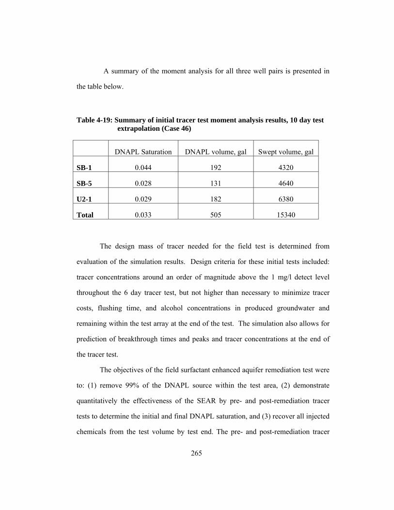
265
A summary of the moment analysis for all three well pairs is presented in
the table below.
Table 4-19: Summary of initial tracer test moment analysis results, 10 day test extrapolation (Case 46)
DNAPL Saturation DNAPL volume, gal Swept volume, gal
SB-1 0.044 192 4320
SB-5 0.028 131 4640
U2-1 0.029 182 6380
Total 0.033 505 15340
The design mass of tracer needed for the field test is determined from
evaluation of the simulation results. Design criteria for these initial tests included:
tracer concentrations around an order of magnitude above the 1 mg/l detect level
throughout the 6 day tracer test, but not higher than necessary to minimize tracer
costs, flushing time, and alcohol concentrations in produced groundwater and
remaining within the test array at the end of the test. The simulation also allows for
prediction of breakthrough times and peaks and tracer concentrations at the end of
the tracer test.
The objectives of the field surfactant enhanced aquifer remediation test were
to: (1) remove 99% of the DNAPL source within the test area, (2) demonstrate
quantitatively the effectiveness of the SEAR by pre- and post-remediation tracer
tests to determine the initial and final DNAPL saturation, and (3) recover all injected
chemicals from the test volume by test end. The pre- and post-remediation tracer

266
tests were essential for fulfilling the second objective. The Phase II test July ‘96
design is summarized in the figure below.
Figure 4-59: Phase II Test Design Summary
The pre-and post-remediation tracer test designs were optimized with a
series of simulation cases. Design parameters included injection and production
rates, tracer injection concentrations, number and partitioning coefficients for the
tracers. The aquifer model was adjusted in a short history match phase (only five
runs made over a one week period), after the initial field tracer test was analyzed, to
better match aquifer-model-predicted and actual-field-observed tracer concentration
effluent curves, initial swept pore volumes, and the calculated DNAPL distribution.
Day:
Pre-Test Inj.
Pre-Remediation Tracer Test
Surfactant Remediation
Post-Test Extraction
Water injection
Tracer injection
2.5 pv surf. inj., plus IPA and NaClExtraction only, no inj.
Injection rate: 2.5 gpm/wellExtraction rate: 3.7 gpm/well150% over-production ratioHydraulic control well rate: 7 gpm/well
1 2 3 4 5 6 7 8 9 10 11 12 13 14 15 16 17 18 19 20 21 22 23 24 25 26 271 2 3 4 5 6 7 8 9 10 11 12 13 14 15 16 17 18 19 20 21 22 23 24 25 26 27
Add NaCl
Tracer injection
Post-Remediation Tracer Test

267
Typically, the history match phase would involve more time and cases; however, in
this case, time was limited and critical parameters (such as DNAPL volume, tracer
breakthrough times and peaks) already matched well.
For the initial tracer test, 2-Propanol was recommended as the conservative
tracer and 1-Pentanol and 2-Ethyl-1-butanol were recommended as the partitioning
tracers at recommended concentrations of 1600 mg/L, 1300 mg/L, and 1300 mg/L,
respectively. The estimated cost for these three tracers for injection in the three wells
during the initial tracer test is shown below:
Tracer Name Cost per kg Design Amount Cost
2-Propanol (K=0.1) $ 31 26.2 kg $ 812
1-Pentanol (K=3.9) $ 19 21.3 kg $ 405
2-Ethyl-1-butanol (K=11.4) $ 66 21.3 kg $ 1406
For the pre-remediation tracer test, 2-Propanol was recommended as the
conservative tracer and 1-Pentanol and 2-Ethyl-1-butanol were recommended as the
partitioning tracers. The recommended concentrations were 1500 mg/L for all three
tracers. The estimated cost for these three tracers for injection in the three wells
during the pre-remediation tracer test is shown below:
Tracer Name Cost per kg Design Amount Cost
2-Propanol (K=0.1) $ 31 25 kg $ 775
1-Pentanol (K=3.9) $ 19 25 kg $ 475
2-Ethyl-1-butanol (K=11.4) $ 66 25 kg $ 1650

268
For the planned post-remediation tracer test for performance assessment, 1-
propanol was recommended as the conservative tracer and 1-hexanol and 1-heptanol
were recommended as the partitioning tracers, at a recommended concentration of
750 mg/L. 1-Proponal was used rather the 2-proponal (IPA) because substantial 2-
proponal was injected as part of the surfactant remediation mix and so could still be
present in the test area during the final tracer test. The tracer concentrations were
lower for this final test because of the lower solubility for the higher partitioning
tracer coefficients (this required a correspondingly longer injection period). The
estimated cost for these three tracers for injection in the three wells during the post-
remediation tracer test is shown below:
Tracer Name Cost per kg Design Amount Cost
1-Propanol (K=0.1) $ 31 31 kg $ 960
1-Hexanol (K=30) $ 21 31 kg $ 650
1-Heptanol (K=141.5) $ 59 31 kg $ 1830
The timing recommended for the Phase II test design was:

269
Test
Segments:
• pre-test flushing (0.5 days)
• tracer injection (0.4 days))
• water flushing (3.6 days)
• flushing with NaCl (1.0 days)
• surfactant/IPA/NaCl injection (3.2 days in all three test area inj. wells)
• water flushing (5.3 days)
• tracer injection (1.0 days)
• water flushing (5.0 days)
• post-test extraction only (4 days)
The design rates and tracers selected were:
Rates: • 11.1 gpm total extraction (for 3 test area producers, 150% over-production)
• 7.5 gpm injection (for 3 test area injectors) plus 7 gpm injection in SB-8,
the hyd. control well.

270
Tracers • non-partitioning tracers:
Bromide, K=0
2-Propanol, K=0 (pre-remediation tracer test)
1-Propanol, K=0 (post-remediation tracer test)
• partitioning tracers:
1-Pentanol, K=3.9 (pre-remediation tracer test)
2-Ethyl-1-butanol, K=12.5 (pre-remediation tracer test)
1-Hexanol, K=30.2 (post-remediation tracer test)
1-Heptanol, K=140.5 (post-remediation tracer test)
Pre-remediation tracer test design and simulation results
Figures in the next section, which covers surfactant remediation test design,
show the DNAPL saturation distribution of the beginning of the pre-remediation and
post-remediation tests. The lowest three layers contain DNAPL and additional
DNAPL is located higher in the structure in the area of U2-1. The region of the test
area just downstream of the SB-2 injector is virtually devoid of DNAPL, as it has
been recovered during the Phase I test. These DNAPL distributions developed in the
simulation model proved very useful in understanding and interpreting the results of
the field tracer tests.

271
Table 4-20: Summary of results for simulation pre-remediation tracer test
U2-1 SB-1 SB-5 IPA residence time, days, 1.50 1.31 1.39 1-Pentanol residence time, days
1.65 1.48 1.53
IPA Tracer breakthrough, hours
<1 2 <1
IPA peak 330 270 290 IPA Tracer recovery 110.6% 88.4% 95.0% 1-Pentanol Tracer recovery 110.4% 88.2% 95.5%
Well Extraction Rate, gpm: 3.7 3.7 3.7
* Breakthrough is here considered to be calculated concentrations greater than 1
mg/l, the measurement lower limit.
** Tracer recoveries are at 8.5 days.
The tracer peak is lowered by the over-production conditions, where the
injection rate is only 2/3 of the production rate.
Figure 4-78 shows the small dissolution of contaminant at the beginning of
the pre-remediation tracer test. This is a plan view of each of the six aquifer model
layers. There is reduced contaminant concentration around all the producers and
injectors, due to TOC dissolution from the multiple pore volumes of water flowing
through the near wellbore volume during the surfactant injection pilot test. Also, the
lowest two layers show significant VOC removal between wells SB-2 and SB-1
from the 6 hours of surfactant injected in SB-1 during the pilot injection test.

272
Table 4-21: Sampling schedule for pre-remediation tracer test
The table above shows the sampling schedule developed for the design of the
field pre-remediation tracer test. The frequency and timing were chosen based on
simulation predicted tracer breakthroughs, peaks, rate of change in concentrations,
and declines to below-detect level concentrations.
WellsTest Segment
Start-End, days
Sampling Frequency,
hoursTotal Number of Samples
Extraction Wells Pre-Test Flushing 0.0 - 0.5 4 9
(U2-1, SB-1, SB-5)Tracer Injection 0.5 - 2.4 1 137and Extraction 2.4 - 5.5 2 112
Test ArrayPre-Test Flushing 0.0 - 0.5 4 3
Monitoring WellTracer Injection 0.5 - 2.4 1 46
(SB-6) and Extraction 2.4 - 5.5 2 37
OutlyingPre-Test Flushing 0.0 - 0.5 24 1
Monitoring WellsTracer Injection 0.5 - 2.4 8 11
(UR-33R and U2-32) and Extraction 2.4 - 5.5 8 19
Total: 374

273
Post-remediation tracer test design and simulation results
Figure 4-69, Figure 4-70, and Figure 4-71 show the predicted effluent tracer
concentrations for the three extraction wells during the post-remediation tracer tests.
Based upon these results, the following sample plan (see table below) was developed
for the field design. These simulation results will be discussed in more detail in
Section 4.3.3, the field results comparison.
Table 4-22: Sampling schedule for post-remediation tracer test
WellsTest Segment
Start-End, days
Sampling Frequency,
hoursTotal Number of Samples
Extraction Wells Tracer Test 14.0 - 16.5 1 180
(U2-1, SB-1, SB-5) 16.5 - 20.0 2 126Post-Test Extraction 20.0 - 24.0 8 36
Test ArrayTracer Test 14.0 - 16.5 1 60
Monitoring Well 16.5 - 20.0 2 42
(SB-6) Post-Test Extraction 20.0 - 24.0 8 12
OutlyingTracer Test 14.0 - 16.5 8 15
Monitoring Wells 16.5 - 20.0 8 21(UR-33R and U2-32)
Post-Test Extraction 20.0 - 24.0 24 8
Total: 500

274
Table 4-23: Design injection and extraction rates, for pre- and post-remediation tracer tests
Figure 4-60 shows the distribution of the non-partitioning tracer at the end of
tracer injection for the post-remediation tracer test. The tracer covers virtually the
entire volume of the lowest three layers, where the DNAPL is concentrated. In
addition, around the SB-3/U2-1 prod./inj. pair (on the left or east side of the pattern),
where DNAPL contaminates higher layers as well, there is also substantial tracer in
the upper layers. The contaminant distribution for each of these layers is shown in
Figure 4-78, for the beginning of the pre-remediation tracer test.
Extraction Rates Injection Rates
Test Segment
Inj. Perioddays
Start-End, days
U2-1 gpm
SB-1 gpm
SB-5 gpm
SB-6 gpm
Total gpm
SB-3 gpm
SB-2 gpm
SB-4 gpm
SB-8 gpm
Total gpm
Pre-Test Flushing 0.5 0.0 - 0.5 3.7 3.7 3.7 0 11.1 2.5 2.5 2.5 7 14.5
Tracer Test 5.0 0.5 - 5.5 3.7 3.7 3.7 0 11.1 2.5 2.5 2.5 7 14.5
Surfactant Injection and Extraction 8.5 5.5 - 14.0 3.7 3.7 3.7 0 11.1 2.5 2.5 2.5 7 14.5
Tracer Test 6.0 14.0 - 20.0 3.7 3.7 3.7 0 11.1 2.5 2.5 2.5 7 14.5
Post-Test Extraction 4.0 20.0 - 24.0 5 5 5 5 20 0 0 0 0 0

275
Layer 1 Layer 2 Layer 3
xxxxxxxxxhill 47b.c 9.t05 xxxxxxxxx hill47b. c9. t05hill47b.c9.t05
xxxxxxxxx
Figure 4-60: Predicted 1-proponal tracer distribution at the end of tracer injection, 15 days, during the
post-remediation tracer test, Layers 1-6, Case 47
During the multiple design simulations, the length of time needed for water
injection after tracer injection was optimized: long enough for good moment analysis
and removal of injected chemicals, while as short as possible to minimize total test
time, sampling, and project costs. Figure 4-61, below, shows the minimal amount of
partitioning tracer remaining in the aquifer at the end of the test. Virtually the entire
test volume is flushed of the injected tracer chemical.
1-Proponal Tracer Concentration, mg/l
0 50 100 150 200 250 300 350 400 450 500 550 600 650 700 750
N
E
S
W
Layer 4 Layer 5 Layer 6
hill 47b.c9.t05hill 47b.c9.t05

276
Figure 4-61: Predicted 1-heptanol tracer concentration distribution at the end of the post-
remediation tracer test and water flushing (24 days), Case 47
The tables below summarize the results of the two final simulation
design cases and the moment analyses conducted on the simulation results.
1-Heptanol Concentration, mg/l
Light blue shaded area envelops all 1-heptanol concentrations greater than 1 mg/L. Transparent areas of mesh represent aquifer with concentrations lower than 1 mg/L
Note:
0 10 20 30 40 50 60 70 80 90 100
U2-1
SB-1
SB-5
SB-3
SB-2
SB-4
EAST hill 47b.c11.t20

277
Table 4-24: Predicted test area pore volumes from moment analysis
Simulation Case 46 & 47 U2-1 SB-1 SB-5 Total Initial tracer test moment analysis pore volumes, gallons:
6,562 4,507 4,772 15,841
Well extraction rate, gpm: 3.0 2.5 2.5 8.0
Post-remediation tracer test moment analysis pore volumes, gallons:
5,180 4,142 4,492 13,814
Well extraction rate, gpm: 3.7 3.7 3.7 11.1

278
Table 4-25: Moment Analysis Summary of Three Predicted Tracer Tests
Initial Tracer Test: U2-1 SB-1 SB-5 Total DNAPL vol., gallons 196 197 123 516
DNAPL saturation 0.045 0.051 0.020 0.036
Swept aquifer vol., gallons 4288 3897 6293 14478
Phase II Initial Tracer Test: U2-1 SB-1 SB-5 Total
DNAPL vol., gallons 26 40 43 109
DNAPL saturation 0.007 0.009 0.008 0.0079
Swept aquifer vol., gallons 3802 4361 5637 13800
Phase II Final Tracer Test: U2-1 SB-1 SB-5 Total
DNAPL vol., gallons 0.0 4.5 1.3 5.8
DNAPL saturation 0.0000 0.0009 0.0002 0.0004
Swept aquifer vol., gallons 4360 4838 6017 15215
% recovery, Phase I and Phase II:
98.9%
% recovery, Phase II Only: 94.6%

279
4.4.2 TRACER TEST EXECUTION AND FIELD RESULTS
Initial tracer test field results
The schedule, chemicals, pore volumes and rates for the initial field tracer
test are in the table below. Table 4-28 shows the results of the moment analysis for
Well SB-1, SB-5 and U2-1. The upper graph in Figure 4-63 shows the Well SB-1
field measured produced tracer concentrations for the non-partitioning tracer IPA
and the lowest partitioning tracer 1-pentanol. These are the two tracers used in the
moment analyses. Field measured data is shown as discrete points, simulation data
as continuous lines. The lower graph in Figure 4-63 shows the produced
concentrations for the two higher partitioning tracers, 2-ethyl-1-butanol and 1-
heptanol. The upper graph in Figure 4-64 shows the Well SB-5’s field measured
produced tracer concentrations for the non-partitioning tracer IPA and the lowest
partitioning tracer 1-pentanol, with the lower graphs showing the same data for Well
U2-1.

280
Table 4-26: Field Initial Tracer Test: Summary
Duration (days)
Cumulative time
(days)
Segment
Chemicals added to Hill source water
2.5 2.5 water flooding
0.5 3.0 tracer injection 1780 mg/L isopropanol (K=0)
1210 mg/L 1-pentanol (K=3.9)
1170 mg/L 2-ethyl-1-butanol (K=12.5)
800 mg/L 1-heptanol (K=140.5)
5.5 8.5 water flooding
0.6 9.1 surfactant/alcohol flooding
8% sodium dihexyl sulfosuccinate, injected in SB-2 only
8.5 17.6 water flooding
2.4 29.7 extraction only
Notes: All injected solutions are mixed in site tap water. The total injection
rate was 1.6 m3/s (7.8 gpm) for all three injectors and the total extraction rate
was 1.4 m3/s (6 gpm) for all three extractors. The water injection rate for the
hydraulic control well SB-8 was 1.4 m3/s (6 gpm).
A large suite of tracers with a very wide range of partitioning values were
chosen for this initial test, as the DNAPL saturation within each inj./prod. pair swept
volume was extremely uncertain and could vary from near zero to above residual
saturation.
The 2-propanol/1-pentanol tracer pair were chosen for this analysis, with
the results extrapolated through 10 days, for consistency with the surfactant
remediation segment injection volume throughput.

281
Sources of error and uncertainty in partitioning tracer tests include:
± extrapolation errors
± moment analyses uncertainties
+ test volume invaded by DNAPL but not contacted by tracer
± tracer conc. measurement errors
Based on an analysis of the uncertainties in column tracer tests
(Dwarakanath, 1997), the uncertainty in the retardation of the partitioning tracer
ranges from ±0.010 to ±0.035. Using this value, upper and lower boundary
saturations and DNAPL volumes may be calculated for the results of the initial
tracer test. The results are summarized in the table below and are shown in detail in
Table 4-28: Initial Tracer Test: Summary of Field Results. Based on this analysis, the
initial DNAPL volume from the partitioning tracer test is 516 gallons, ±120 gallons
(±23%).
Table 4-27: Initial DNAPL volume, with uncertainty range, for the initial Phase II tracer test
From Moment Analysis: Lower Range
Calc. Value Upper Range
initial tracer test DNAPL volume, gallons
393 516 637
difference in gallons: -123 121
percentage difference: -24% 23%
The 11.5 day test (plus 6 days for pre- and post-flushing) was carried out
successfully in May 1996. Based on moment analyses of the tracer test results, the
total DNAPL contacted was 516 gallons, and the total swept aquifer volume was

282
14,500 gallons, for a contacted DNAPL saturation of 0.036 within the test array area.
The tracer residence time ranged from 1.4 to 2.2 days for the IPA tracer. Tracer
breakthrough times for the three extraction wells ranged from 4 to 11 hours.
Surfactant breakthrough times ranged from 4 to 24 hours and surfactant peaks
ranged from 0.07 to 0.80 wt.%. The total contaminant recovered during the May ‘96
test was 192 gallons, 107 gallons as DNAPL and 85 gallons as contaminant
dissolved in the aqueous phase.
The extraction rates during the test averaged around 3.0, 2.4, and 2.4 gallons
for Wells U2-1, SB-1, and SB-5, respectively, for a total extraction rate of 7.8 gpm.
The injection rates were 2.0 gpm per well, for a total test array injection rate of 6
gpm. This is an overproduction ratio of 7.8/6, or 130%. Including the hydraulic
control well SB-8, which injected water at a rate of 6 gpm throughout the test, the
total injection rate was 12 gpm.
Figure 4-62 is a photograph of the test site at Hill OU2 during the Phase I May
1996 Test. The 3x3 well array plus the mid-array monitoring well were under the
striped tent. The tracers and surfactant solutions were mixed in the 4 tanks to the
right of the tent.

283
Figure 4-62: Equipment configuration for field site tracer and surfactant tests

284
Table 4-28: Initial Tracer Test: Summary of Field Results
U2-1 SB-1 SB-5 Total DNAPL vol., gallons 195.7 196.7 123.4 515.8
DNAPL saturation 0.045 0.051 0.020 0.036
Swept aquifer vol., gallons 4288 3897 6293 14478
IPA residence time, days, 1.41 1.45 2.18 1.68
1-Pentanol residence time, days 1.57 1.70 2.28 1.85
IPA Tracer breakthrough, hours 5 4 11 7
IPA peak 310 350 300 320
IPA Tracer recovery 98% 86% 92% 92%
Pentanol Tracer recovery 95% 86% 87% 89%
Surf. Breakthrough, hours 10 4 24 13
Surf. Peak, wt.% 0.13% 0.80% 0.07% 0.33%
Surfactant recovery 5% 64% 3% 72%
Contaminant recovered as dissolved phase, gallons
6.1 49.0 6.8 61.9
Contaminant recovered as DNAPL, gallons
- 107.0 - 107.0
Total Contaminant Recovered, gallons
6.1 156.0 6.8 168.9
Well Extraction Rate, gpm: 3.0 2.4 2.4 7.8
Determination of swept and DNAPL volumes from tracer tests
There can be significant differences between the swept or actual ‘test area’
volume and the expected ‘test area’ volume. The expected ‘test area’ volume is that
bounded by the line of injection in the south, in the north by the extraction wells, and

285
the aquitard the east, west, and beneath. These differences are due to the effect of
reservoir heterogeneities, rates, partial completions of the aquifer thickness, and well
configuration. Certainly, the pore volumes of water passing through lower
permeability zones will be fewer than those passing through the higher permeability
zones, but given (1) a long enough test, (2) not too severe variation in permeability,
and (3) a proper well configuration, the tracer should sweep all zones -- these again
are design/aquifer variables that can be very usefully examined with a 3-dimensional
heterogeneous simulation model.
With good site characterization and careful simulation, tracer breakthroughs,
peaks, and non-partitioning tracer concentrations may be predicted accurately. What
cannot be routinely predicted in tracer tests are retardation, peaks, and ‘tails’ of
partitioning tracer produced concentrations, since the DNAPL saturation has a strong
effect on these and is unknown before the tracer test analysis. However, in this
study, the initial volume of DNAPL estimated in the aquifer model agreed quite
closely well with that calculated by analysis of the Phase I field test. This estimated
initial DNAPL distribution in the aquifer simulations was based primarily on VOC
soil content measurements and the aquitard structure, but also included evaluation of
the DNAPL pumping history of test area wells, historical dissolved concentrations in
wells near the test area. This is discussed in later sections.
The 57,000 L swept pore volume corresponds to an estimated 6.7 m x 6.1 m
x 4.0 m swept test volume. These estimated dimensions are based upon evaluation of
the simulation results, since it would be prohibitively expensive to place sufficient
monitoring wells to determine precise boundaries of ‘swept volume’ for the field
test. The ‘expected’ test area is 6.1 m x 5.4 m x 4.9 m, but of course, in this

286
unconfined, heterogeneous field scale test with irregular boundaries, some
streamlines pass slightly outside or inside of this test volume. The thickness of the
saturated aquifer varies from 2.7 m to 6.1 m within the test area. However, the wells
are screened only in the lowest 3 m of the aquifer and the production and injection
tubing is placed within the lowest 0.15 m of the aquifer; so the streamlines are
concentrated in the lower portion of the aquifer, rather than sweeping the entire
vertical thickness evenly.
Hydraulic control
Based on measured tracer concentrations, 97% of the tracers injected during
the two weeks of the initial tracer test were recovered. This high recovery in a short
time would have been quite impossible without hydraulic confinement of the test
area. If any streamlines passed from the injectors to outside of the pattern area, the
recovery of the injected tracers would have been much lower. This is the primary
confirmation and best means of determining the degree of hydraulic control;
however, the achievement of hydraulic control in the tracer tests can also be
supported by three other sources of information: Firstly, measured piezometric data
during the tests indicated that water levels for the three extraction wells were
approximately a meter lower than the surrounding aquifer, creating a large gradient
from within the test area towards the extraction wells. Secondly, monitoring wells
were placed both to the north and south of the test array (aquitard confines aquifer to
the east and west). These monitoring wells produced at undetectable or extremely
low concentrations of the injected tracer throughout the test, with peak
concentrations around the detection level of the GC, less than 1% of the injected

287
concentration. These monitoring wells were approximately 21 meters away from
the pattern, far enough away that any streamlines escaping the pattern and containing
tracer would diffuse/disperse through most of the narrow aquifer channel. Thirdly,
the simulation results matched the model very well in predicted tracer recovery (both
were 97% for the initial tracer test) and other key parameters such as breakthroughs
and peaks, indicating that the simulator is a reliable model of actual field
performance. The simulations showed very low final concentrations for all injected
chemicals in all gridblocks outside the pattern.
Pre-remediation tracer test
The schedule, chemicals, pore volume and rates for the pre-remediation field
tracer test are summarized in the table below. Three tracers were injected in all three
injection wells at a concentration ranging from 1140 to 1560 mg/l, for 10 hours or
0.3 pv of the test pattern volume. Injection rates were 7.5 gpm. Total extraction
rates were 9.2 gpm for the 3 pattern wells, for an over-production ratio of 123%.
The hydraulic control well injected at a rate of 7 gpm; considering this well also in
the total pattern rates results in over-injection conditions, at a ratio of 158% The
calculated DNAPL volumes and saturations, from moment analysis of the tracer test
concentrations, are also shown in the table below.
The actual measured concentrations for the field pre-remediation tracer test
are shown in Figure 4-66, Figure 4-67, and Figure 4-68 for the extraction wells SB-1, SB-
5, and U2-1, respectively. Tracer breakthrough occurred within 4 to 11 hours, with
the peak tracer concentrations occurring a few hours after tracer injection stopped.
The “straight-line” behavior, necessary for effective moment analysis, began within

288
a day of the peak concentrations. Tracer recovery at 8.5 days ranged from 92% for
the conservative tracer and 89% for the partitioning tracer 1-pentanol.
Table 4-29: Summary of field results for pre-remediation tracer test
U2-1 SB-1 SB-5 Total IPA residence time, days, 1.41 1.45 2.18 1.68 1-Pentanol residence time, days
1.57 1.70 2.28 1.85
IPA Tracer breakthrough, hours *
5 4 11 7
IPA peak 310 350 300 320 IPA Tracer recovery ** 98% 86% 92% 92% 1-Pentanol Tracer recovery** 95% 86% 87% 89%
Well Extraction Rate, gpm: 3.1 3.1 3.1 9.2
U2-1 SB-1 SB-5 Total
DNAPL vol., gallons 26 40 43 109
DNAPL saturation 0.007 0.009 0.008 0.0079
Swept aquifer vol., gallons 3802 4361 5637 13800
* Breakthrough is here considered to be calculated concentrations greater than 1
mg/l, the measurement lower limit.
** Tracer recoveries are at 8.5 days.
Table 4-32 reports the final measured tracer concentrations for the pre- and
post-remediation field tracer tests. After only 6 days, the pre-remediation
partitioning tracers 1-pentanol and 2-ethyl-1-butanol had dropped to only 1% of their
injection concentrations. Though not measured, after a further 20 days of injection

289
and extraction, these tracer concentrations would undoubtedly be below detect
levels.
Post-remediation tracer test
The schedule, chemicals, pore volumes, and rates for the post-remediation
field tracer test are summarized in Table 4-31. Four tracers were injected in all three
pattern injectors, for 24 hours, or 0.3 pv of the test pattern, at concentrations ranging
from 430 to 860 mg/l. The concentrations were lower for this tracer test compared
to previous ones because the higher partitioning tracers needed for this final test had
a lower solubility; therefore the injection period was higher, for a roughly equivalent
mass of tracer injected. The rates were the same as for the pre-remediation test. The
field measured produced tracer concentrations are shown in Figure 4-69, Figure 4-70,
and Figure 4-71. The small separation observed between the tracer curves (which
would suggest that DNAPL remains within the pattern area) is actually a result of
differing injection concentrations. When the produced tracer curves are instead
plotted as normalized concentrations, by dividing the produced tracer concentrations
by the injected concentrations, it is evident that the concentrations overlay, within
measurement variations expected under field conditions.
The results of the moment analysis for this tracer tests are summarized in
Table 4-37, with the top third containing the field results. DNAPL saturations less
than 0.001 were calculated for all wells, for a total test volume remaining DNAPL
volume of 6 gallons.
Based on an analysis of the uncertainties in column tracer tests
(Dwarakanath, 1997), the uncertainty in the retardation of the partitioning tracer

290
ranges from ±0.010 to ±0.035. The initial DNAPL volume from the partitioning
tracer test is 516 gallons, ±120 gallons (±23%). The final DNAPL volume from the
partitioning tracer test is 6 gallons, ±3 gallons (±50%), Table 4-30. Therefore, the
estimated field test DNAPL recovery ranges from 97.5% to 99.4%, with a mean
estimated value of 98.8%
Table 4-30: Summary of DNAPL volumes calculated from initial and final tracer test moment analyses
From Moment Analysis: Lower Range
Calc. Value Upper Range
initial tracer test DNAPL volume, gallons
393 516 637
difference in gallons: -123 121
percentage difference: -24% 23%
final tracer test DNAPL volume, gallons
4 6 10
difference in gallons: -3 4
percentage difference: -43% 61%

291
Table 4-31: Measured field injection concentrations, pre- and post-remediation tracer tests
Seg. Time days
Total Time days
Segment
Pore Vol.
Chemicals added to Hill source water
1.7 1.7 water flooding 1.2 0.4 2.1 tracer injection 0.3 1,558 mg/L isopropanol
1,234 mg/L 1-pentanol 1,137 mg/L 2-ethyl-1-butanol
3.7 5.8 water flooding 2.6 1.0 6.8 NaCl preflood 0.7 7,000 mg/L NaCl 3.4 10.2 surfactant/alcohol
flooding 2.4 7.55% sodium dihexyl
sulfosuccinate 3.75 % isopropanol 7,000 mg/L NaCl
11.0 21.2 water flooding 7.8 1.0 22.2 tracer injection 0.7 855 mg/L 1-propanol
431 mg/L bromide 800 mg/L 1-hexanol 610 mg/L 1-heptanol
5.1 27.3 water flooding 3.6 2.4 29.7 extraction only --
Notes: 1. All injected solutions are mixed in Hill tap water.
2. The total injection rate was 1.7 m3/s (7.5 gpm) for all three injectors and the
total extraction rate was 2.1 m3/s (9.2 gpm) for all three extractors.
3. The water injection rate for the hydraulic control well SB-8 was 1.6 m3/s (7
gpm).
The table below reports the final measured pre- and post-remediation field
tracer tests. At the end of the field test, 7.6 days after tracer injection ends, the
measured concentrations of the post-remediation tracers were only 0.7-1.2% of the
injected concentrations, ranging from 3 to 19 mg/l.

292
Table 4-32: Final field measured tracer concentrations, from onsite gc measurements
4.4.3 COMPARISON WITH SIMULATION RESULTS
Initial tracer test and Simulation Case 46
The predicted aquifer model concentrations shown here are those developed
before the test was undertaken and, therefore, are not history-matched or calibrated
to the field data. Even so, breakthrough times, peaks, and tails for both the
g
Chemicals U2-1 SB-1 SB-5 AverageInjected or Initial
% of Initial or Inj.
Tracers:mg/l
1-Pentanol 13 9 16 13 1226 1.0%
mg/l (8/11/96) (8/12/96) (8/12/96) (after 6 days)
2-Ethyl-1-butanol 13 10 19 14 1146 1.2%
mg/l (8/11/96) (8/12/96) (8/12/96) (after 6 days)
1-Propanol 6 10 3 6 891 0.7%
mg/l (9/2/96) (9/2/96) (9/2/96) (test end)
1-Hexanol 5 6 4 5 676 0.7%
mg/l (9/2/96) (9/2/96) (9/2/96) (test end)
1-Heptanol
mg/l

293
partitioning and non-partitioning tracers are remarkably similar for the UTCHEM
prediction and field results.
Table 33 and 34 compare the actual Phase I Field Test performance with the
UTCHEM simulation Case 46. Figure 4-63 and Figure 4-64 compare predicted
performance for Case 46 and the actual field performance. In general, tracer
breakthroughs and tracer peak times matched very well. As shown in Figure 4-63, for
Wells SB-1, predicted and field observed breakthrough times and peak times
matched within hours for all four tracers. The measured peak concentrations for the
field test were generally 10% to 20% higher than the simulation concentrations, with
correspondingly higher tracer recovery for this well in the field compared to the
aquifer model. The upper graph in Figure 4-64 compares the predicted and field
measured tracer concentrations for Well SB-5. The breakthroughs and peaks occur
much earlier in the aquifer model compared to the field, suggesting a smaller pore
volume between the inj./prod. pair in the model compared to the field. This is
consistent with the calculated swept pore volume from the moment analysis of SB-5,
where the simulation volume of 4641 gal is 36% less than the calculated volume of
6293 gal from the field results (Table 4-34). In contrast, the swept volumes for the
SB-1/SB-2 well pair for field vs. simulation results were much closer, within 10%.
Interestingly, both the aquifer model and the field tracer curves show a slight
bimodal character, only for the SB-5/SB-4 well pair, indicating a more marked
variation in stream tubes arrival for this well (and a corresponding geometry?)
compared to the other well pairs.

294
Figure 4-63: Comparison of field vs. simulation produced tracer concentration for initial tracer test, Well SB-1
0
50
100
150
200
250
300
350
0 1 2 3 4 5 6
Pred. 2-ethyl-1-butanol (K=12.5)Field 2E1BPredicted 1-heptanol (K=140.5)Field 1-heptanol
conc
entra
tion,
mg/
l
Days
0
50
100
150
200
250
300
350
400
450
500
0 1 2 3 4 5 6
Predicted IPA (K=0)Field IPAPredicted 1-pentanol (K=3.9)Field 1-pentanol
conc
entra
tion,
mg/
l

295
Figure 4-64: Comparison of field vs. simulation produced tracer concentration for initial tracer
test, Well SB-5 and U2-1
0
50
100
150
200
250
300
350
0 1 2 3 4 5 6
predicted IPA (K=0)Field IPApredicted 1-pentanol (K=3.9)Field 1-pentanol
conc
entra
tion,
mg/
l
Days
0
50
100
150
200
250
300
350
400
0 1 2 3 4 5 6
predicted IPA (K=0)Field IPApredicted 1-pentanol (K=3.9)Field 1-pentanol
conc
entra
tion,
mg/
l
Days

296
Table 4-33: Comparison of Field and Simulation Results for Initial Tracer Test
Field Results U2-1 SB-1 SB-5 Total
IPA Tracer breakthrough, hours
5 4 11 7
IPA peak 310 350 300 320
IPA Tracer recovery 98% 86% 92% 92%
Pentanol Tracer recovery 95% 86% 87% 89%
Simulation Results (C46) U2-1 SB-1 SB-5 Total
IPA Tracer breakthrough, hours
5 5 3 4
IPA peak 335 285 305 308
IPA Tracer recovery 109% 81% 82% 91%
Pentanol Tracer recovery 109% 78% 79% 89%
Difference U2-1 SB-1 SB-5 Total
IPA Tracer breakthrough, hours
5% 20% -267% -51%
IPA peak (normalized) 7% -23% 2% -4%
IPA Tracer recovery 10% -6% -12% -1%
Pentanol Tracer recovery 12% -10% -9% -1%
Notes: 1. Reported tracer recoveries are based upon performance up to 6 days of the test, with no extrapolation.

297
Table 4-34: Comparison of Field and Simulation Results for Initial Tracer Test Moment Analysis
Field U2-1 SB-1 SB-5 Total DNAPL vol., gallons 195.7 196.7 123.4 515.8
DNAPL saturation 0.045 0.051 0.020 0.036
Swept aquifer vol., gal. 4288 3897 6293 14478
Simulation Case 46 U2-1 SB-1 SB-5 Total DNAPL vol., gallons 182.4 191.6 131.0 505.0
DNAPL saturation 0.029 0.044 0.028 0.033
Swept aquifer vol., gal. 6,380 4,315 4,641 15,336
Difference U2-1 SB-1 SB-5 Total DNAPL vol., gallons -7% -3% 6% -2%
DNAPL saturation -57% -14% 31% -8%
Swept aquifer vol., gal. 33% 10% -36% 6%
Notes: 1. Calculated volumes based on moment analysis for the IPA-Pentanol tracer pair. 2. Calculated volumes based upon performance up to 6 days of the test, with extrapolation of extraction well concentrations to 10 days, corresponding to the surfactant remediation segment of the field test.
For Well U2-1 (lower graph in Figure 4-64) the tracer peaks times and values
and curve shapes are similar for the aquifer model and the field test, particularly for
the non-partitioning tracer IPA.
Overall, the aquifer model total test area DNAPL volumes, saturations, and
swept aquifer volumes are within 2 to 8% of the field results, as shown in the last
column of Table 4-34. This match was achieved as the result of a very short (1
week) history matching process. Individual prod./inj. well pair results could have

298
been more closely matched, with additional work, if it were necessary for the
subsequent field test, and if time and resources were available. However, even
before history matching, the aquifer modeled predicted the field performance quite
accurately, as can be seen by reviewing simulation cases executed before the field
tests were conducted. Two of these cases are discussed in the next two sections.
Initial tracer test and published work plan Phase I Case, Prediction Case 17
The objectives of our use of a complex three-dimensional multi-phase multi-
component simulator were to (1) design the field tests, and (2) accurately predict the
performance of field tests before they were conducted, and (3) interpret the results of
the field test. For the first two objectives, simulation results and comparisons with
field data reported here are based on these simulation design studies conducted
before the field tests were executed. As no field test has ever been executed exactly
as designed in every detail, there are some differences in simulations compared to
those for the actual field test, primarily in well average rates and fluctuations, and
test segment timings. However, any predictions presented to clients, regulators, and
other decision makers who must judge whether or not to approve the test can be
based only on what is known before the test is conducted. Therefore, it is of great
importance that simulations conducted before the test be able to predict such critical
parameters as injected chemical recovery, hydraulic confinement, and DNAPL
recovery.
Most remediation simulations presented in the literature are ‘predictions’
conducted after the test has been completed -- actually ‘history’ rather than
‘prediction’ simulations. It is, of course, much easier to ‘predict’ field test or

299
laboratory test performance after the test has already occurred and is known, but
accurate pre-test modeling is essential to convince regulators and other stakeholders
that the test will safely achieve its objectives and should be approved. However,
these post-test simulations, with rates and other conditions adjusted to those from the
actual field test, can be of great utility for examining in detail the aquifer behavior
and remediation performance. The value of these simulations can be increased
further by calibrating or ‘history-matching’ the model to better match actual field
performance (measured concentrations, DNAPL produced, water levels, DNAPL
and swept volumes from tracer tests), by adjusting the many parameters in the model
with substantial uncertainty, such as stratigraphy and structure; aquifer permeability
and initial DNAPL distribution; longitudinal and transverse dispersivity, porosity,
relative permeability, capillary pressure, capillary desaturation, and their variation
throughout the aquifer; surfactant/water/contaminant/electrolyte phase behavior, and
well performance. Such a history-matching process involves a large manpower and
time investment and could not be done in the three months between the Phase I and
Phase II field tests, as this time was needed for collating, analyzing, and evaluating
the results of the Phase I test. Fortunately, the Phase I design predicted overall test
performance very well, including such key results as injected chemical recovery,
breakthrough times, flushing times, peaks, etc. and only minor changes were made in
the simulations for the Phase II prediction simulations. However, the effort to
history-match the current aquifer model could be of great value in examining
remediation processes in detail or for designing further remediation tests at Hill
AFB.

300
The primary criteria for successful test design are fulfillment of the most
important test objectives. Such fulfillment requires the ability to predict field
performance – before the test is conducted. Figure 4-65 compares the results of the
aquifer model prediction case presented in March ‘96 to AFCEE, before the test was
conducted, to the measured May ‘96 Phase I Field Test results. Table 4-35
compares the actual field performance to the predicted performance for UTCHEM
Case 17, the ‘workplan’ case.
Figure 4-65: Comparison of field vs. model-predicted produced tracer concentration for pre-remediation
tracer test, Well SB-1, “Work plan” Case 17
0
50
100
150
200
250
300
350
400
0 1 2 3 4 5 6
UTCHEM IPAField IPA, K=0UTCHEM 1-pentanolField 1-pentanol, K=3.9
Con
cent
ratio
n, m
g/l
Days
0
50
100
150
200
250
300
350
400
0 1 2 3 4 5 6
UTCHEM IPAField IPA, K=0UTCHEM 1-pentanolField 1-pentanol, K=3.9
0
50
100
150
200
250
300
350
400
0
50
100
150
200
250
300
350
400
0 1 2 3 4 5 60 1 2 3 4 5 6
UTCHEM IPAField IPA, K=0UTCHEM 1-pentanolField 1-pentanol, K=3.9
UTCHEM IPAField IPA, K=0UTCHEM 1-pentanolField 1-pentanol, K=3.9
Con
cent
ratio
n, m
g/l
Days

301
The following table compares the predicted and actual Phase I test
performance:
UTCHEM Predicted Actual
IPA Tracer Recovery, % 92 92
Surfactant Recovery, % 78 72
VOC Recovery, gallons 78 169
DNAPL from PITT, gallons 508 515
Table 4-35: Comparison of Field and Simulation Results for Initial Tracer Test, published workplan.
Field U2-1 SB-1 SB-5 Total
DNAPL vol., gallons 195.7 196.7 123.4 515.8
DNAPL saturation 0.045 0.051 0.020 0.036
Swept aquifer vol., gallons
4288 3897 6293 14478
Prediction Case 17 U2-1 SB-1 SB-5 Total
DNAPL vol., gallons 13 338 178 529
DNAPL saturation 0.003 0.081 0.042 0.041
Swept aquifer vol., gallons
4629 4197 4209 13035
Difference U2-1 SB-1 SB-5 Total
DNAPL vol., gallons 93% -72% -44% -3%
DNAPL saturation 93% -60% -114% -14%
Swept aquifer vol., gallons
-8% -8% 33% 10%
Notes:

302
1. Calculated volumes based on moment analysis for the IPA-Pentanol tracer pair. 2. Calculated volumes based upon performance up to 6 days of the test, with extrapolation of extraction well concentrations to 10 days, corresponding to the surfactant remediation segment of the Phase II test.
Intermediate Phase I simulation case 28cd
The table below compares the field performance to aquifer model Case 28,
which is identical to Work Plan Case 17 except that the rates were adjusted to match
actual field rates and phase behavior was adjusted for consistency with measured in
situ test temperatures, around 12°C, whereas Case 17 phase behavior was based on
data measured at ambient laboratory conditions of 23°C.

303
Table 4-36: Comparison of Field and Simulation Results for Initial Tracer Test Moment Analysis, Work Plan Case, except rates and temperatures adjusted to actual field conditions
Field U2-1 SB-1 SB-5 Total
DNAPL vol., gallons 195.7 196.7 123.4 515.8
DNAPL saturation 0.045 0.051 0.020 0.036
Swept aquifer vol., gallons
4288 3897 6293 14478
Prediction Case 28 U2-1 SB-1 SB-5 Total
DNAPL vol., gallons 168.4 242.8 106.7 517.9
DNAPL saturation 0.032 0.061 0.027 0.039
Swept aquifer vol., gallons
5304 3978 3930 13212
Difference U2-1 SB-1 SB-5 Total
DNAPL vol., gallons -16% 19% -16% 0%
DNAPL saturation -41% 17% 28% 9%
Swept aquifer vol., gallons
19% 2% -60% -10%
Notes: 1. Calculated volumes based on moment analysis for the IPA-Pentanol tracer pair. 2. Calculated volumes based upon performance up to 6 days of the test, with extrapolation of extraction well concentrations to 10 days, corresponding to the surfactant remediation segment of the Phase II test.
Pre-remediation tracer test and simulation Case 46

304
Figure 4-66 through Figure 4-68 compare the aquifer model predicted and
field test measured concentrations and moment analysis results for the pre-
remediation field test. A comparison of arrival times between the field and model
results shows results similar to the initial tracer time, with peak magnitude matching
very well for all three wells, and the Well SB-5 peak arrival time around a half day
earlier in the model compared to actual field results.
Figure 4-66: Comparison of field vs. model-predicted produced tracer concentration for pre-remediation tracer test, Well SB-1

305
Figure 4-67: Comparison of field vs. model-predicted produced tracer concentration for pre-
remediation tracer test, Well SB-5
1
10
100
1000
0 1 2 3 4 5
Predicted IPA (K=0)
Field IPA
Predicted 1-pentanol (K=3.87)
Field 1-pentanolco
ncen
trat
ion,
mg/
l
Daystracer inj. begins (0.5 days)tracer inj. ends (0.9 days)Surf. inj. begins (5.5 days

306
Figure 4-68: Comparison of field vs. model-predicted produced tracer concentration for pre-remediation tracer test, Well U2-1
Post-remediation tracer test and simulation Case 47
The table below and Figure 4-69 through Figure 4-71 compare the model-
predicted and field measured results for the post-remediation tracer tests. In both the
model and the field, very little separation in the partitioning and non-partitioning
tracers occurs, indicating graphically the low remaining DNAPL saturation at the
end of the test (consistent in the field and in the aquifer model). The remaining
DNAPL predicted by the model was a total of 6.8 gallons, which is very close to the
5.8 gallons determined by moment analysis of the field measured data.
The upper graphs in Figures 4-69 through 4-71 show the field and model
concentrations in mg/l, for a partitioning and non-partitioning tracer, for each
extraction well. The lower graphs in each of the figures are normalized
1
10
100
1000
0 1 2 3 4 5
Predicted IPA (K=0)Field IPAPredicted 1-pentanol (K=3.87)Field 1-pentanol
conc
entr
atio
n, m
g/l
tracer inj. begins (0.5 days)tracer inj. ends (0.9 days)
Surf. inj. begins (5.5 days)Days

307
concentrations, field measured data only. For wells SB-5 and U2-1, all normalized
tracer concentrations virtually overlay, within the uncertainty of the data. Only for
Well SB-1 is there significant separation or retardation for the partitioning tracer
data, and only for the highest partitioning coefficient tracer, n-Heptanol, K=140.5.
Table 4-37: Comparison of post-remediation tracer test moment analysis: field vs. simulation
Field Results U2-1 SB-1 SB-5 Total
DNAPL vol., gallons 0.0 4.5 1.3 5.8
DNAPL saturation 0.0000 0.0009 0.0002 0.0004
Swept aquifer vol., gallons 4,360 4,838 6,017 15,215
Simulation Results (C47) U2-1 SB-1 SB-5 Total
DNAPL vol., gallons 2.1 4.0 0.6 6.8
DNAPL saturation 0.0004 0.0010 0.0001 0.0005
Swept aquifer vol., gallons 5,275 4,111 4,481 13,866
Difference U2-1 SB-1 SB-5 Total
DNAPL vol., gallons 98% -12% -101% 14%
DNAPL saturation 98% 5% -50% 21%
Swept aquifer vol., gallons 17% -18% -34% -10%
Notes: 1. Calculated volumes based on moment analysis for the 1-Proponal/1-Heptanol tracer pair.
2. Calculated volumes based upon performance up to 6 days of the test, with extrapolation of extraction well concentrations to 8.5 days, corresponding to the surfactant remediation segment of the Phase II test.

308
Figure 4-69: Comparison of field vs. model-predicted produced tracer concentration for post-
remediation tracer test, Well SB-1
0.001
0.01
0.1
1
0 1 2 3 4 5 6 70.001
0.01
0.1
1
0.001
0.01
0.1
1
0 1 2 3 4 5 6 70 1 2 3 4 5 6 7
Nor
mal
ized
Con
cent
ratio
n
Time, days
n-Hexanol, K=30
n-Heptanol, K=140.5
Bromide
IPA, K=0

309
Figure 4-70: Comparison of field vs. model-predicted produced tracer concentration for post-remediation tracer test, Well SB-5
1
10
100
1000
14 15 16 17 18 19 20Days
Predicted 1-ProponalField 1-ProponalPredicted 1-hexanol (K=30.2)Field 1-Hexanol
conc
entra
tion,
mg/
l
0.001
0.01
0.1
1
0 1 2 3 4 5 6 7
Nor
mal
ized
Con
cent
ratio
n
Time, days
n-Heptanoln-Hexanol
n-Propanol
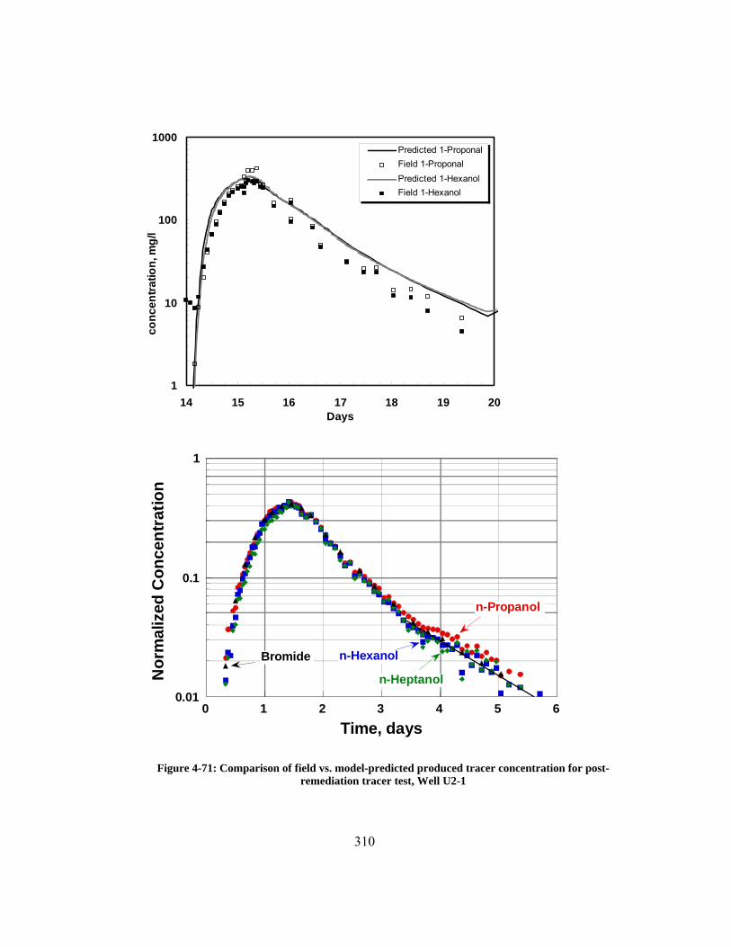
310
Figure 4-71: Comparison of field vs. model-predicted produced tracer concentration for post-
remediation tracer test, Well U2-1
1
10
100
1000
14 15 16 17 18 19 20Days
Predicted 1-ProponalField 1-ProponalPredicted 1-HexanolField 1-Hexanol
conc
entra
tion,
mg/
l
0.01
0.1
1
0 1 2 3 4 5 6
Nor
mal
ized
Con
cent
ratio
n
Time, days
n-Propanol
n-Heptanol
Bromide n-Hexanol

311
4.5 SURFACTANT REMEDIATION
4.5.1 REMEDIATION DESIGN AND MODEL PREDICTED PERFORMANCE
The objectives for the pilot surfactant injection test (Phase I) and the
surfactant remediation test (Phase II) were considerably different. The primary
objective of the surfactant remediation test was to remove essentially all of the
DNAPL present in the test area within a 30 day period, with secondary objectives as
mentioned at the beginning of this chapter. The 11.5 day surfactant injection pilot
test (plus 6 days for pre- and post-flushing) was carried out successfully in May
1996, producing approximately 170 gallons of contaminant in the form of DNAPL
and dissolved VOCs.
The surfactant injection pilot test, “Phase I”, had only 0.1 pv of 8%
surfactant injected, with no added NaCl. The Surfactant Enhanced Aquifer
Remediation (SEAR) field test, “Phase II”, had 2.4 pv injection of 8% surfactant,
with added NaCl.
A series of simulation cases were conducted to study the effect of well,
reservoir, fluid, and simulation parameters upon predicted pilot and SEAR tests
performance. The objectives of these simulations were to:
• Determine length of time required for each segment of the test: tracer
injection, post-tracer water-flushing, surfactant injection, polymer injection,
post-SEAR water-flushing, etc.
• Determine whether adding polymer improves the performance by increasing
conformance and/or decreasing test length needed to sweep all zones.

312
• Determine mass of tracers, surfactant, polymer, and electrolytes
recommended for each segment of the tests.
• Determine test design parameters such as number of hydraulic control and
injection and production wells needed; injection and production rates, etc.
• Estimate produced concentrations of contaminant, tracers, surfactant,
polymer, and electrolytes.
• Estimate mass of contaminant, tracers, surfactant, polymer, and electrolytes
that remain in the aquifer, either within the pattern or migrating outside, after
each test ends.
• Evaluate effects of mesh, aquitard structure, boundaries, and well design
upon test performance, migration of DNAPL, production of solubilized
versus free phase contaminant, etc.
• Evaluate effects of surfactant phase behavior, fluid properties, sorption,
concentration gradients, etc.
• Evaluate effects of uncertainties in permeability distribution upon surfactant
and tracer performance.
Pilot Surfactant Injection Test Design
The following design for the pilot surfactant injection test was based on a
series of simulations using the aquifer model: A solution of 8% sodium dihexyl
sulfosuccinate surfactant mixed in source water (by weight) was injected for 0.6
days (14 hours), in one well only, Well SB-2, the central injection well, across from
extraction well SB-1. The mass of surfactant required for this injection was 523
kilograms of active surfactant. As sodium dihexyl sulfosuccinate was only available

313
on an 80% active basis, 654 kilograms or 1440 lbs of sodium dihexyl sulfosuccinate
(the commercial name of the product used is Aerosol MA-80I) was be needed.
Somewhat more than the 1440 lbs calculated was ordered to allow for various
practical storage, mixing and injection considerations. This is 1728 gallons of 8%
surfactant solution and approximately 0.1 pv, based on the total test swept array pore
volume, or 0.3 pv of the pore volume swept by the SB-2/SB-1 well pair. During the
surfactant injection in Well SB-2, water was injected in wells SB-3, SB-4, and SB-8,
to maintain the flow fields and to confine the injected surfactant streamlines within
the test array volume. All three extraction wells also continued pumping during this
period, at a rate of 3 gpm/well.
Following the 0.6 day surfactant injection, water was injected in all three test
array wells, for 4.4 days (2.4 pv), to recover the surfactant.
Sampling schedule plan
During the first 2.5 days of the surfactant injection segment, all three
extraction wells were planned to be sampled approximately every 30 minutes, to
allow for precise determination of DNAPL and dissolved contaminant and surfactant
concentrations, including breakthroughs, peaks, and cumulative recoveries.
Determination of the total mass of surfactant recovered allows estimation of the
amount of surfactant remaining in the aquifer after the test ends and, by comparison
with the tracer recovery, the amount of surfactant adsorbed.
During the last 2.5 days of the surfactant injection segment, the planned
sampling frequency was reduced to once every hour. This results in a total of 180
samples per extraction well over the 5 day surfactant injection segment.

314
The monitoring well should be sampled more frequently at the beginning of
this segment, approximately twice as often as for extraction wells if practicable, until
the of DNAPL and surfactant breakthroughs and peaks were observed and the
surfactant and dissolved contaminant concentrations decline to low levels. Well SB-
6 was monitored more frequently than the extraction wells as it lies directly in the
path between the surfactant injection Well SB-2 and its extraction well, SB-1. The
sampling of SB-6 is in one respect even more important than that for the extraction
wells, as it will be more indicative of actual test array in situ surfactant and dissolved
contaminant concentrations. Due to the ‘over-production’ design, Well SB-1 and the
other extraction wells will produce test array fluids significantly diluted by inflowing
groundwater. The planned sampling frequency for Well SB-6 was every 30 minutes
during the first day of the surfactant segment, then once an hour for the next day,
then once every four hours for the last 3 days of the surfactant segment.
Sampling intervals of only once per day were recommended for the two
monitoring wells outside the test array.
Aquifer model results
Figure 4-72 through Figure 4-82 show aquifer model simulation distributions of
contaminant, microemulsion, and surfactant, for vertical cross-sections, areal layers,
and 3-D sections. Figure 4-100, Figure 4-101, and Figure 4-102 illustrate the model
predicted produced surfactant and contaminant concentrations, for Wells SB-1, SB-
5, and U2-1, respectively. The aquifer model simulation results are shown as
smooth curves; the field test measured results are shown as discrete points, and will
be discussed in subsequent sections.

315
During the first six days of the Phase I Pilot Test, during the tracer test, the
effluent surfactant concentration is zero and the effluent contaminant concentration
is equal to the solubility in groundwater, 1100 mg/L. Surfactant is injected
beginning at 6 days and ending at 6.6 days (approx. 14 hours, 0.3 pv of the inj/ext
well pair pv). The surfactant concentration versus time plot (Figure 4-100) shows a
sharp peak where concentration increases rapidly, followed by rapid decrease, then a
long 'tail' where the concentration decreases gradually. The surfactant breaks
through almost immediately after injection begins, as the wells are very close
together. The peak simulation surfactant concentration is only 1.2%, substantially
below the 8% injected concentration, because only a small volume (0.3 pv) of
surfactant is injected and because dilution by groundwater occurs and is increased by
the 50% over-production conditions. The produced surfactant concentration has
dropped below 1% only 1 day after surfactant injection ends.
The organic contaminant effluent concentration versus time is shown in
Figure 4-100, lower graph, for Well SB-1. The predicted contaminant concentration
peaks at 2000 mg/L, corresponding to the peak in surfactant concentration reaching
the extraction well. The concentration decreases to the aqueous solubility (1100
mg/L) once the surfactant concentration drops below the CMC, the critical micellar
concentration, here estimated at 0.2% surfactant concentration. This occurs
approximately 3.9 days after surfactant injection ends (at 10 days in Figure 4-100).
Figure 4-72 and Figure 4-73 show the change in predicted contaminant
distribution throughout the pilot test, for a vertical cross-section through the central
inj./prod. pair, for six different times. Surfactant injection begins at 6.0 days, the end
of the initial tracer test. At this time DNAPL exists as residual saturation (red zones)

316
in the lower three layers of the aquifer, with lower saturations where the highest pore
volumes have previously flushed the aquifer: injection Well SB-2, just downstream
of this well in the bottom layer, and around extraction Well SB-1. After 6 hours of
injection (at 6.3 days), this flushed zone has expanded and in addition a small bank
of mobilized DNAPL (dark red zone, indicates saturation higher than the residual
0.25) between SB-6 and SB-1, flows towards and is produced by extraction Well
SB-1. At the end of the surfactant injection phase (6.6 days), the zone between
injection Well SB-2 and observation Well SB-6 has been virtually cleansed of
contaminant, and this contaminant has been mobilized and moved as a small bank
towards extraction Well SB-1. At the end of the test (15 days), the mobilized
DNAPL has been produced. Only a very small pulse (0.3 pv) of surfactant has
solubilized / mobilized around half of the contaminant between SB-1 and SB-2.
However, the real extent of this removal is very small, as can be observed in Figure
4-76. This shows the areal contaminant distribution for the lowest three layers of the
aquifer, at 6.0 days and 6.6 days, the beginning and end of the surfactant injection
phase. Contaminant (the red zones) remains distributed throughout the aquifer
except for the small region immediately surrounding SB-2 and SB-6. The
contaminant distribution at the end of the pilot test, for all six layers of the aquifer
model, is shown in Figure 4-80. This remaining contaminant is the target of the
second phase of the test, the SEAR, where several pore volumes are injected in all
three injectors of the test pattern.
The surfactant distribution is shown in Figure 4-74. After half the surfactant in
injected (at 6.3 days), the surfactant is distributed between injection Well SB-2 and
monitoring Well SB-6, concentrated in the lower layers, at near the injection

317
concentration of 8% (indicated as red zones). At the end of the 14 hour surfactant
injection pulse, the surfactant also sweeps the region between monitoring Well SB-6
and extraction Well SB-1. After 12 hours of water flushing, most of the surfactant
has been removed from the aquifer, produced to extraction Well SB-1. In Figure 4-75,
the scale has been expanded (with a maximum concentration of 1% rather than 8%)
to highlight the areas where even low concentrations of surfactant persist. After 1
day of water flushing (at 7.6 days), the lower layers have been swept but surfactant
takes longer to sweep contaminant from the lower layers. The areal extent of the
surfactant, for all six layers of the aquifer model, can be observed in Figure 4-78, at the
end of the surfactant injection period, at 6.6 days. At the end of the water flushing
(11 days), most of this surfactant has been recovered, with concentrations around the
0.2 wt.% CMC (the green zones) around Well SB-6. At the end of the pilot test (15
days) with four additional days of extraction only, the only region where surfactant
concentrations exceeds the CMC is between injection Well SB-2 and hydraulic
control Well SB-8, where these two adjacent injectors create a low velocity
“stagnation zone” between these wells.
The microemulsion distribution throughout the aquifer, at the end of the
surfactant injection (at 6.6 days) is shown in Figure 4-77. Wherever the surfactant
concentration in Figure 4-78 is greater than 0.2 wt.%, an aqueous phase microemulsion
forms and replaces the aqueous phase. Figure 4-82 shows the 3-D distribution of
surfactant remaining in the aquifer at the end of the pilot test, 15 days. This small
mass of surfactant, which would otherwise be biodegraded and dissipated over time,
is removed during the second phase of the field project, the SEAR, discussed in the
next section.

318
No electrolytes are added to the fluids injected during the Phase 1 Pilot Test.
Produced electrolytes are a mixture of the source water and ground water
constituents.
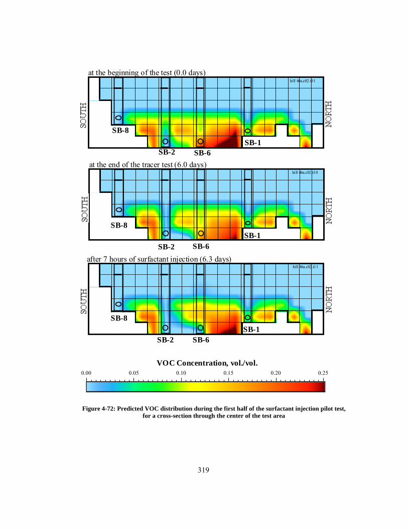
319
Figure 4-72: Predicted VOC distribution during the first half of the surfactant injection pilot test, for a cross-section through the center of the test area
SB-8
SB-2 SB-6SB-1
after 7 hours of surfactant injection (6.3 days)
at the end of the tracer test (6.0 days)
at the beginning of the test (0.0 days)
SB-2 SB-6SB-1
SB-8
SB-8
SB-2 SB-6SB-1
hill 46a.c02.t01
hill 46a.c02.t10
hill 46a.c02.t11
0.00 0.05 0.10 0.15 0.20 0.25VOC Concentration, vol./vol.

320
Figure 4-73: Predicted VOC distribution during the second half of the surfactant injection pilot
test, for a cross-section through the center of the test area, Case 46
0.00 0.05 0.10 0.15 0.20 0.25
SB-8
SB-2 SB-6SB-1
at the end of the Phase I test (15 days)
at the end of the Phase I water flushing (11 days)
at the end of the surfactant injection (6.6 days)
SB-2 SB-6SB-1
SB-8
SB-8
SB-2 SB-6SB-1
hill 46a.c02.t12
hill 46a.c02.t16
hill 46a.c02.t17
VOC Concentration, vol./vol.

321
Figure 4-74: Predicted surfactant distribution during the first half of the surfactant injection pilot
test, for a cross-section through the center of the test area, Case 46
0 1 2 3 4 5 6 7 8
SB-8
SB-2 SB-6SB-1
after 12 hours of waterflushing (7.1 days)
at the end of the 14 hour surfactant injection segment (6.6 days)
after 7 hours of surfactant injection (6.3 days)
SB-2 SB-6SB-1
SB-8
SB-8
SB-2 SB-6SB-1
hill 46a.c3.t11
hill 46a.c3. t12
hill 46a.c3.t13
Surfactant Concentration, wt%

322
Figure 4-75: Predicted surfactant distribution during the last half of the surfactant injection pilot test, for a cross-section through the center of the test area (expanded concentration scale), Case 46
0.0 0.1 0.2 0.3 0.4 0.5 0.6 0.7 0.8 0.9 1.0
SB-8
SB-2 SB-6SB-1
at the end of the Phase I test (15 days)
at the end of the Phase I waterflushing (11 days)
after 1 day of waterflushing (7.6 days)
SB-2 SB-6SB-1
SB-8
SB-8
SB-2 SB-6SB-1
hill 46a.c3.t14
hill 46a.c3.t16
hill 46a.c3.t17
Surfactant Concentration, wt%

323
Figure 4-76: Predicted contaminant distribution at 6.0 and 6.6 days (after 2.4 hours and at the end of
surfactant injection), Layers 4-6, Case 46
Layer 4 Layer 5 Layer 6
hill 46a.c2.t10 hill 46a.c2.t10 hill 46a.c2.t10
SB-1
SB-2
SB-6
6.0 Days:
Contaminant Concentration, vol./vol.0.00 0.05 0.10 0.15 0.20 0.25
Layer 4 Layer 5 Layer 6
N E
S W
hill 46a.c2.t12 hill 46a.c2.t12 hill 46a.c2.t12
6.0 Days:

324
Figure 4-77: Predicted microemulsion distribution at the end of surfactant injection (6.6 days), Layers 2-6, Case 46
Layer 1 Layer 2 Layer 3
xxxxxxxxx hill46a. s3. t12hill46a.s3.t12hill 46a.s3.t12
Layer 1
xxxxxxxxxhill 46a.c3.t12
Microemulsion Saturation, vol./vol.
0.00 0.10 0.20 0.30 0.40 0.50 0.60 0.70 0.80 0.90 1.00
Layer 4 Layer 5 Layer 6
N
E
S
W
hill 46a.c3.t12 hill 46a.c3.t12 hill 46a.c3.t12

325
Figure 4-78: Predicted surfactant distribution at the end of surfactant injection (6.6 days), Layers 1-6, Case 46
Layer 1 Layer 2 Layer 3
xxxxxxxxx hill46a. c3. t12hill46a.c3.t12hill 46a.c3.t12
Surfactant Concentration, wt%
0 1 2 3 4 5 6 7 8
Layer 4 Layer 5 Layer 6
N
E
S
W
hill 46a.c3.t12 hill 46a.c3.t12 hill 46a.c3.t12

326
Figure 4-79: Predicted 3-D surfactant distribution at the end of surfactant injection (6.6 days), Case
46
Surfactant Concentration, wt%
Note: Light blue shaded area envelopes all aquifer areas with surfactant concentrations greater than the CMC (0.2 wt%) required for microemulsion formation. Transparent areas of mesh represent aquifer with concentrations below the 0.2 wt% CMC.
0 1 2 3 4 5 6 7 8
U2-1
SB-1
SB-5
SB-3
SB-2
SB-4
hill 46a. c3 .t12EAST

327
Figure 4-80: Predicted contaminant distribution at the end the surfactant injection pilot test (15 days), Layers 1-6, Case 46
Layer 1 Layer 2 Layer 3
xxxxxxxxx hill46a. c2. t17hill46a.c2.t17hill 46a.c2.t17
Contaminant Concentration, vol./vol.0.00 0.05 0.10 0.15 0.20 0.25
Layer 4 Layer 5 Layer 6
N
E
S
W
hill46a. c2. t17hill46a.c2.t17hill 46a.c2.t17

328
Figure 4-81: Predicted 3-D DNAPL distribution at the end of the surfactant injection pilot test (15 days), Case 46
DNAPL Saturation, vol./vol.
Light blue shaded area envelopes all DNAPL saturations greater than 0.006. Transparent areas of mesh represent aquifer with saturations lower than 0.006.
Note:
0.00 0.05 0.10 0.15 0.20 0.25
hill 46a. s2.t17
U2-1
SB-1
SB-5
SB-3
SB-2
SB-4
EAST

329
Figure 4-82: Predicted 3-D surfactant distribution at the end of the surfactant injection pilot test (15 days), Case 46
hill 46a. c3.t17
U2-1
SB-1
SB-5
SB-3
SB-2
SB-4
EAST
Surfactant Concentration, wt%
Note: Light blue shaded area envelopes all aquifer areas with surfactant concentrations greater than the CMC (0.2 wt%) required for microemulsion formation. Transparent areas of mesh represent aquifer with concentrations below the 0.2 wt% CMC.
0 1 2 3 4 5 6 7 8

330
Evolution of the Phase II Design and Aquifer Model
The objectives of the Phase II SEAR test were to: (1) remove as much as
possible of the DNAPL remaining within the test area after Phase I, and (2)
demonstrate the effectiveness of the SEAR by following it with a tracer test to
determine the remaining DNAPL saturation.
A multitude of simulation cases have been conducted to develop the
recommended designs summarized here for the Phase I and Phase II site field tests.
These have allowed the study of the effect of such design variables as rates for the
extraction and injection wells, the effect of the hydraulic control well upon
confinement, the effect of polymer in improving sweep efficiency, and the effect of
increasing the amount of surfactant in increasing the contaminant recovery. The
phase behavior parameters were modified to match solubility to the anticipated
aquifer temperature, approximately 12 °C, rather than the laboratory ambient
temperature, approximately 23 °C.
Surfactant Injection
Based on a pore volume of 1,600 cubic feet (47,000 liters) and about 2 pore
volumes of surfactant/alcohol injection, the quantity of surfactant, polymer and
alcohol are shown below. This calculation is based on 4% sodium dihexyl
sulfosuccinate and 8% IPA. Additionally, 10,000 mg/l of NaCl added to the source
water is required to achieve the Type III microemulsion phase behavior.

331
Amount of surfactant (MA-80I) kilograms
Amount of Alcohol kilograms
Amount of Polymer kilograms
5,000 5,500 0
The final Phase II SEAR test design developed consisted of:
Test
Segments:
• pre-test flushing (0.5 days)
• flushing with NaCl (1.0 days)
• surfactant/IPA/NaCl injection (3.0 days in all three test area inj. wells)
• water flushing (5.5 days)
• tracer injection (0.5 days)
• water flushing (5.5 days)
• post-test extraction only (4 days)
The design rates were:
Rates: • 11.1 gpm total extraction (for 3 test area producers, 150% over-
production)
• 7.5 gpm injection (for 3 test area injectors) plus 7 gpm injection in SB-8,
the hyd. control well.
The quantity and distribution of DNAPL within the test area was unknown
before the Phase I pilot test. This test allowed the determination of the volume of
DNAPL within the test area, and, since there were multiple injector/producer pairs,
the general distribution of DNAPL within the test area, providing a better design for
the Phase II SEAR test.

332
Phase II Surfactant Remediation Test Simulation Results
Figure 4-83 through Figure 4-92 show the predicted contaminant, surfactant, and
chloride concentrations and the DNAPL and microemulsion saturation distribution
maps, for cross-sections of the model and the full three dimensions of the grid.
Figure 4-104 and 4-105 show the predicted effluent contaminant and surfactant
concentrations versus time for Well SB-1. Well SB-5 predicted performance is
shown in Figure 4-107, Well U2-1 in Figure 4-107. The moment analyses for the
three extraction wells for the Prediction Case 47 pre-remediation tracer test, before
the surfactant remediation, is illustrated in Figures 4-65 through 4-67 and
summarized in Table 4-37. The moment analyses for the three extraction wells for
the Prediction Case 47 post-remediation tracer test, after the surfactant remediation,
is illustrated in Figures 4-69 through 4-71 and summarized in Table 4-37.
Figure 4-84 is a three-dimensional representation of the DNAPL saturation
within the model grid at the beginning of Phase II. The lowest three layers contain
DNAPL and additional DNAPL is located higher in the structure in the area of U2-1.
As shown in this figure, the region of the test area just downstream of the SB-2
injector is virtually devoid of DNAPL, as it has been recovered during the Phase I
test.
Figure 4-87 portrays the distribution of surfactant predicted by UTCHEM at
the end of the Phase II surfactant injection segment. To allow visualization of the
regions of the aquifer containing surfactant, all aquifer gridblocks with surfactant
concentrations less that the CMC (critical micelle concentration) of 0.20 wt% have
been rendered transparent. After three days of injection of a source water containing

333
8% surfactant in all three injectors, surfactant has reached all three extraction wells
and is distributed throughout the test area. The presence of the hydraulic control
Well SB-8 to the south of the test area and the three extraction wells bounding the
northern edge of the test area provide the hydraulic control needed to keep the
surfactant within the test area. The steeply sloping sides of the clay aquitard to the
east and west of the test area and the considerable thickness of the clay zone below
the test area further serve to confine the injected chemicals and mobilized DNAPL.
Figure 4-104 shows the predicted contaminant concentration produced by
Well SB-1 during Phase II. The black line represents the total produced
contaminant, in mg/l. Before surfactant injection, the dissolved VOC is 1100 mg/l,
the solubility of the site VOC mixture in groundwater with no added surfactant; this
is equivalent to 4 gpd of VOC recovery, dropping slightly below this as some of the
streamtubes pass through clean aquifer. Twelve hours after surfactant injection
begins, DNAPL breaks through at this extraction well and peaks at 12,000 mg/l
(over 50 gpd DNAPL recovery rate). This is followed by VOC dissolved in the
microemulsion phase. The surfactant injection stops after 3 days and the produced
contaminant continues to decline. The VOC recovery drops further as the few
remaining zones with DNAPL in the test area are flushed. However, the produced
VOC concentration would not drop to zero, even with 100% contaminant recovery
within the test area, as contaminated groundwater enters the extraction well from the
substantial unremediated areas outside the test area.
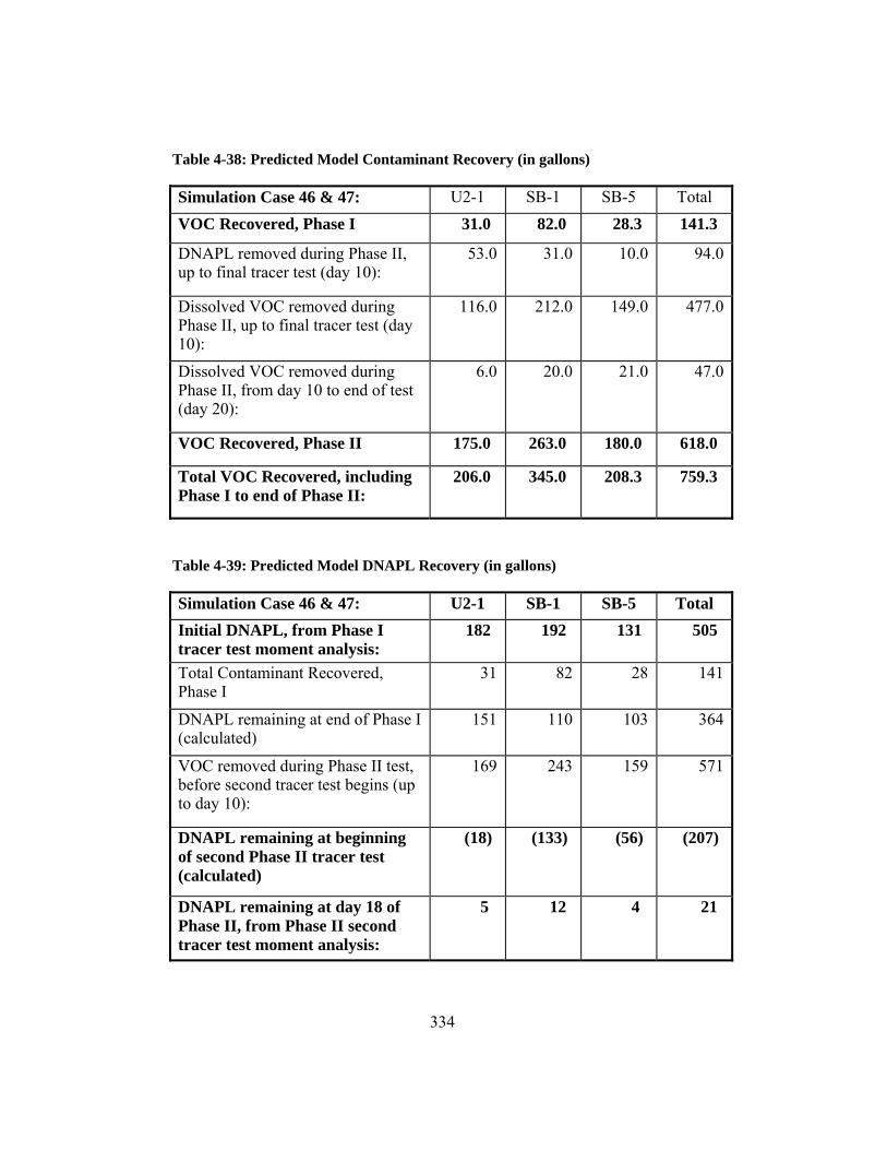
334
Table 4-38: Predicted Model Contaminant Recovery (in gallons)
Simulation Case 46 & 47: U2-1 SB-1 SB-5 Total VOC Recovered, Phase I 31.0 82.0 28.3 141.3
DNAPL removed during Phase II, up to final tracer test (day 10):
53.0 31.0 10.0 94.0
Dissolved VOC removed during Phase II, up to final tracer test (day 10):
116.0 212.0 149.0 477.0
Dissolved VOC removed during Phase II, from day 10 to end of test (day 20):
6.0 20.0 21.0 47.0
VOC Recovered, Phase II 175.0 263.0 180.0 618.0
Total VOC Recovered, including Phase I to end of Phase II:
206.0 345.0 208.3 759.3
Table 4-39: Predicted Model DNAPL Recovery (in gallons)
Simulation Case 46 & 47: U2-1 SB-1 SB-5 Total Initial DNAPL, from Phase I tracer test moment analysis:
182 192 131 505
Total Contaminant Recovered, Phase I
31 82 28 141
DNAPL remaining at end of Phase I (calculated)
151 110 103 364
VOC removed during Phase II test, before second tracer test begins (up to day 10):
169 243 159 571
DNAPL remaining at beginning of second Phase II tracer test (calculated)
(18) (133) (56) (207)
DNAPL remaining at day 18 of Phase II, from Phase II second tracer test moment analysis:
5 12 4 21

335
Figure 4-83: Predicted contaminant distribution at the beginning of the surfactant enhanced aquifer remediation test, Layers 1-6, Case 47
Layer 1 Layer 2 Layer 3
xxxxxxxxx hill46a. c2. t17hill46a.c2.t17hill 46a.c 2.t17
VOC Concentration, vol./vol.
0.00 0.05 0.10 0.15 0.20 0.25
Layer 4 Layer 5 Layer 6
N
E
S
W
hill 46a.c 2.t17 hill 46a.c 2.t17 hill 46a.c 2.t17
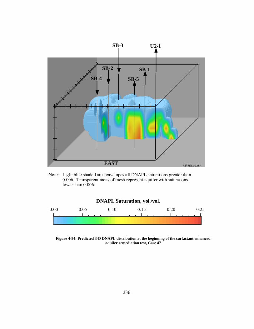
336
Figure 4-84: Predicted 3-D DNAPL distribution at the beginning of the surfactant enhanced
aquifer remediation test, Case 47
DNAPL Saturation, vol./vol.
Light blue shaded area envelopes all DNAPL saturations greater than 0.006. Transparent areas of mesh represent aquifer with saturations lower than 0.006.
Note:
0.00 0.05 0.10 0.15 0.20 0.25
hill 46a. s2.t17
U2-1
SB-1
SB-5
SB-3
SB-2
SB-4
EAST

337
Figure 4-85: Predicted VOC distribution at the beginning of the surfactant enhanced aquifer
remediation SEAR test, for a cross-section through the center of the test area, Case 47
VOC Concentration,vol./vol.
0.00 0.05 0.10 0.15 0.20 0.25
SB-8
SB-2 SB-6SB-1
10 hours of surf. injection (5.9 days)
5 hours of surf.injection (5.7 days)
0 hours of surf.injection (5.5 days)
SB-2 SB-6SB-1
SB-8
SB-8
SB-2 SB-6SB-1
hill 47a.c2.t16
hill 47a.c2.t18
hill 47a.c2.t20

338
Figure 4-86: Predicted VOC distribution during surfactant enhanced aquifer remediation SEAR test, for a cross-section through the center of the test area, Case 47
VOC Concentration,vol./vol.
0.00 0.05 0.10 0.15 0.20 0.25
SB-8
SB-2 SB-6SB-1
at the end of the 3.2 day surf.injection (8.7 days)
1.5 days of surf.injection (7.0 days)
1.0 day of surf. injection (6.5 days)
SB-2 SB-6
SB-1SB-8
SB-8
SB-2 SB-6SB-1
hill 47a.c2.t33
hill 47a.c2.t26
hill 47a.c2.t24

339
Figure 4-87: Predicted 3-D surfactant distribution at the end of surfactant injection (8.7 days), Case 47
Surfactant Concentration, wt%
Light blue shaded area envelopes all DNAPL concentrations greater than 0.002 (0.02%). Transparent areas of mesh represent aquifer with concentrations lower than.002 (0.02%).
Note:
U2-1
0.0 0.5 1.0 1.5 2.0 2.5 3.0 3.5 4.0 4.5 5.0 5.5 6.0 6.5 7.0 7.5 8.0
SB-1
SB-5
SB-3
SB-2
SB-4
hill 47a. c3 .t33EAST

340
Figure 4-88: Predicted 3-D DNAPL distribution at the end of the surfactant enhanced aquifer remediation test ( 24 days), Case 47
Light blue shaded area envelops all DNAPL saturation greater than 0.006 (0.6%). Transparent areas of mesh represent aquifer with concentrations lower than 0.006 (0.6%).
Note:
Predicted DNAPL distribution at the end of the phase II test (24 days) Hill AFB Phase II SEAR Test Case 47
DNAPL Saturation, vol./vol.
13
0.00 0.05 0.10 0.15 0.20 0.25
U2-1
SB-1
SB-5
SB-3
SB-2
SB-4
hill 47b. s2 .t20EAST

341
Figure 4-89: Predicted 3-D surfactant distribution at the end of the surfactant enhanced aquifer remediation test ( 24 days), Case 47
Surfactant Concentration,wt%
Light blue shaded area envelops all surfactant concentrations greater than 0.002. Transparent areas of mesh represent aquifer with concentrations lower than.002.
Note:
0.0 0.5 1.0 1.5 2.0 2.5 3.0 3.5 4.0 4.5 5.0 5.5 6.0 6.5 7.0 7.5 8.0
U2-1
SB-1
SB-5
SB-3
SB-2
SB-4
EAST hill 47b.c3.t20

342
Figure 4-90: Predicted 3-D surfactant distribution at the end of the surfactant enhanced aquifer remediation test, expanded scale ( 24 days), Case 47
Light blue shaded area envelopes all surfactant concentrations greater than 0.01 wt%. Transparent areas of mesh represent aquifer with concentrations lower than 0.01 wt%
Note:
Surfactant Concentration,wt%
CMC (2000 mg/L) 4000 mg/L
0.00 0.04 0.08 0.12 0.16 0.20 0.24 0.28 0.32 0.36 0.40
U2-1
SB-1
SB-5
SB-3
SB-2
SB-4
EAST hill 47b.c3.t20

343
Figure 4-91: Predicted 1-proponal distribution at the end of the Phase II test (24 days), Case 47
Light blue shaded area envelopes all 1-proponal concentrations greater than 1 mg/L. Transparent areas of mesh represent aquifer with concentrations lower than 1 mg/L.
Note:
1-Proponal Concentration, mg/L
0 10 20 30 40 50 60 70 80 90 100
U2-1
SB-1
SB-5
SB-3
SB-2
SB-4
EAST hill 47b.c9.t20

344
Figure 4-92: Predicted 3-D chloride distribution at the end of the surfactant enhanced aquifer remediation test, 4400 mg/L chloride injection concentration, 170 mg/L for source water, 60 mg/L for
groundwater ( 24 days), Case 47
Chloride Concentration, mg/l
0 50 100 150 200 250 300 350
U2-1
SB-1
SB-5
SB-3
SB-2
SB-4
Light aqua shaded area envelopes all chloride concentrations greater than 60 mg/L NaCl. Transparent areas of the mesh represent aquifer with concentrations lower than 60 mg/L.
Note:
hill 47b. c6 .t20EAST

345
4.5.2 REMEDIATION EXECUTION AND FIELD RESULTS
Surfactant Injection Pilot Test Field Results, Phase I
Based on moment analyses of the tracer test results, (see Section 4.4.2 and
4.4.3) the total DNAPL contacted was 516 gallons, and the total swept aquifer
volume was 14,500 gallons, for a contacted DNAPL saturation of 0.036 within the
test array area. Surfactant breakthrough times ranged from 4 to 24 hours and
surfactant peaks ranged from 0.07 to 0.80 wt.%. The total contaminant recovered
during the May ‘96 test was 169 gallons, 107 gallons as DNAPL and 62 gallons as
contaminant dissolved in the aqueous phase.
The extraction rates during the test averaged around 3.0, 2.4, and 2.4 gallons
for Wells U2-1, SB-1, and SB-5, respectively, for a total extraction rate of 7.8 gpm.
The injection rates were 2.0 gpm per well, for a total test array injection rate of 6
gpm, an overproduction ratio of 7.8/6, or 130%. Including the hydraulic control well
SB-8, which injected water at a rate of 6 gpm throughout the test, the total injection
rate was 12 gpm.

346
Table 4-40: Summary of Results for Surfactant Injection Pilot Test
U2-1 SB-1 SB-5 Total
DNAPL vol., gallons 195.7 196.7 123.4 515.8 DNAPL saturation 0.045 0.051 0.020 0.036 Swept aquifer vol., gallons 4288 3897 6293 14478
Surf. Breakthrough, hours 10 4 24 13 Surf. Peak, wt.% 0.13% 0.80% 0.07% 0.33% Surfactant recovery 5% 64% 3% 72%
Cont. recovered as dissolved phase, gallons
6.1 49.0 6.8 61.9
Contaminant recovered as DNAPL, gallons
- 107.0 - 107.0
Total Contaminant Recovered, gallons
6.1 156.0 6.8 168.9
Well Extraction Rate, gpm: 3.0 2.4 2.4 7.8
Notes: 1. Calculated volumes based on moment analysis for the IPA-Pentanol tracer pair. 2. Calculated volumes based upon performance up to 6 days of the test, with extrapolation of extraction well concentrations to 10 days, corresponding to fluid volumes injected in the surfactant remediation segment of the Phase II test.
Test of Surface and Subsurface Equipment
Existing groundwater treatment facilities at Hill AFB OU2, including phase
separators and a steam stripper, the SRS or Source Recovery System, were utilized
to treat all of the groundwater and DNAPL recovered during the surfactant flooding
field tests. Rates produced to the SRS are shown in Figure 4-97. The high levels of
surfactant, salt, IPA, and contaminant (TCE) in the recovered groundwater presented

347
significant challenges for steam stripper operation. The maximum contaminant
concentration of the produced water (total from all three extraction wells) entering
the treatment facility was 9,200 mg/l, compared to an average concentration of 400
mg/l before surfactant injection. Prior to the field tests, predictive modeling
(ASPEN Plus with empirical vapor-liquid-equilibrium data) was used to determine if
and how the existing steam stripper could achieve required cleanup levels (Radian,
1994b). Actual operation of the steam stripper during the field tests demonstrated
that predicted performance levels were achieved.
The favorable operation of existing surface treatment facilities during the
Phase I test demonstrates that steam stripping is a favorable technology for the
treatment of the highly contaminated groundwaters recovered during surfactant
enhanced remediations.
Table 4-41: Initial Concentrations of VOC Contaminants, Surfactant Injection Pilot Field Test, in mg/l
At the beginning of test:
Chemical U2-1 SB-1 SB-5 Average
TCE 260 614 185 346
TCA 40 130 41 68
PCE 13 16 7 12
Sum of the VOCs 313 760 233 426
** Averages are based on the average extraction rate for each well.

348
Table 4-42: Final Concentrations of VOC Contaminants, Surfactant Injection Pilot Field Test, in mg/l
At the end of the test:
Chemical U2-1 SB-1 SB-5 Average
TCE 733 926 184 623
TCA 131 213 43 129
PCE 184 21 8 80
Sum of the VOCs 1048 1160 235 832
** Averages are based on the average extraction rate for each well.
Figure 4-93: Surfactant Injection Pilot Test: Field Measured Temperatures, showing diurnal
variation in aquifer temperature, closely tracking changes in air temperatures
Surfactant Injection Pilot Test: Field Measured Temperatures
5
10
15
20
25
30
35
5/4 5/5 5/6 5/7 5/8 5/9 5/10 5/11 5/12 5/13 5/14 5/15 5/16 5/17 5/18
Tem
pera
ture
°C
U2-1SB-1SB-5INJAir Temp.

349
Figure 4-94: Field produced dissolved contaminant: concentrations, cumulatives, and percentages, Well SB-1, Surfactant Injection Pilot Test.
0
5,000
10,000
15,000
20,000
5/6 5/8 5/10 5/12 5/14 5/16 5/18 5/20 5/22
cont
amin
ant c
once
ntra
tion,
mg/
l
0
20
40
60
80
cum
ulat
ive
diss
olve
d pr
od. c
ont.,
gal
.
dissolved contaminant concentrationcumulative dissolved cont. production
0%
20%
40%
60%
80%
100%
120%
5/6 5/8 5/10 5/12 5/14 5/16 5/18 5/20 5/22
wt.%
of e
ach
cons
titue
nt
%TCE%TCA
%PCE

350
Figure 4-95: Field produced dissolved contaminant: concentrations, cumulatives, and percentages, Well SB-1, Surfactant Injection Pilot Test.
0.0%
0.1%
0.2%
0.3%
0.4%
0.5%
0.6%
0.7%
0.8%
0.9%
1.0%
5/118:00
5/128:00
5/138:00
5/148:00
5/158:00
5/168:00
5/178:00
5/188:00
5/198:00
5/208:00
5/218:00
surfa
ctan
t con
cent
ratio
n, w
t%
0
100
200
300
400
500
600
700
800
900
1,000
cum
ul. s
urf.
reco
very
, lbs
. M
A-8
0
surfactant concentrationcumulative production
surfactant injection: 5/12/96, 8:00 - 22:00
CMC
0
3,000
6,000
9,000
12,000
15,000
18,000
5/118:00
5/128:00
5/138:00
5/148:00
5/158:00
5/168:00
5/178:00
5/188:00
5/198:00
5/208:00
5/218:00
cont
amin
ant c
once
ntra
tion,
mg/
l
dissolved contaminantconcentration
surfactant injection: 5/12/96, 8:00 - 22:00

351
Surfactant Enhanced Aquifer Remediation Field Test, Phase II
The table below is a summary of the segments, injection rates, and chemicals
injected and their concentrations, for the surfactant enhanced aquifer remediation
(SEAR) field test.
Table 4-43: Summary of Phase II Test
Duration (days)
Cumulative time (days)
Segment Pore Volumes
Chemicals added to Hill source water
1.7
1.7 water flooding 1.2
0.4 2.1 tracer injection 0.3 1,572 mg/L 2-propanol (K=0) 1,247 mg/L 1-pentanol (K=3.9) 1,144 mg/L 2-ethyl-1-butanol (K=12.5)
3.7
5.8 water flooding 2.6
1.0
6.8 NaCl preflood 0.7 7,000 mg/L NaCl
3.4 10.2 surfactant/ alcohol flooding
2.4 7.55% sodium dihexyl sulfosuccinate 4.47 % isopropanol 7,000 mg/L NaCl
11.0
21.2 water flooding 7.8
1.0 22.2 tracer injection 0.7 854 mg/L 1-propanol (K=0) 431 mg/L bromide (K=0) 798 mg/L 1-hexanol (K=30) 606 mg/L 1-heptanol (K=141)
5.1
27.3 water flooding 3.6
2.4 29.7 extraction only -- Notes: All injected solutions are mixed in Hill tap water. The total injection rate
was 1.7 m3/s (7.5 gpm) for all three injection wells and the total extraction rate was 2.1 m3/s (9.2 gpm) for all three extraction wells. The water injection rate for the hydraulic control well SB-8 was 1.6 m3/s (7 gpm).

352
Hydraulic Conductivity
There was no loss of hydraulic conductivity as a result of the field test, and
no evidence of significant gel formation or pore blocking. The basis for this
conclusion is that the induced hydraulic gradients (from water level measurements)
between the injectors and producers were the same before and after the test. Water
level depths were measured throughout the tests for the three injection/extraction
well pairs, during Phase I and II (the upper and lower graphs, respectively in Figure
4-96). The hydraulic heads or water level differences (∆h) between each injector
and extraction well were calculated from the measured water levels. Since injection
and production rates were also constant, a loss of hydraulic conductivity as a result
of surfactant would have increased the gradient between the wells (i.e., q=KI)
During Phase I (upper graph), the hydraulic head actually decreased between well
SB-1 and SB-2, as the DNAPL was recovered, reducing the pore blockage and
increasing the relative permeability to water. In Phase II (the lower graph), water
levels increased because the total injection rate, including the hydraulic control well,
was 12 gpm while the extraction rate was only 7.8 gpm.

353
Figure 4-96: Difference in water table depth between test area extraction/injection well pairs,
Phase I and Phase II
Surfactant injection begins
0.0
0.4
0.8
1.2
1.6
0 3 6 9 12 15 18 21 24 27
SB-1/SB-2SB-5/SB-4U2-1/SB-3
Diff
eren
ce in
Dep
th to
Wat
er, m
eter
s
Days8/7/96 9/3/96
Surfactant injection ends
0
0.5
1
1.5
2
2.5
3
3.5
4
4.5
5/2 5/3 5/4 5/5 5/6 5/7 5/8 5/9 5/10 5/11 5/12 5/13 5/14 5/15 5/16 5/17 5/18 5/19 5/20 5/21 5/22
Date
diffe
renc
e in
dep
th to
wat
er ta
ble
bet
wee
n in
ject
or a
nd p
rodu
cer,
in fe
et
∆h SB-5/SB-4∆h SB-1/SB-2∆h U2-1/SB-3
tracer injection surfactant injection Phase I test ends
Water Level Difference Between Injector/Producer Pairs .

354
Although this demonstration was in a relatively small volume of the aquifer,
the swept pore volume of 15,000 gallons is still an order of magnitude greater than
the pore volume of the isolation test cells used at Borden and the LNAPL site at Hill
AFB OU1. This step increase in aquifer volume treated demonstrates substantial
progress in moving from the small-scale laboratory stage towards the ‘full-scale’
field stage, which is, of course, the purpose and ultimate objective of any in situ
remediation technique.
DNAPL Recovery
Table 4-44: Initial and Final DNAPL Volumes and Saturations from Tracer Tests for SEAR Field Test
Well Pair U2-1/SB-3
Well Pair SB-1/SB-2
Well Pair SB-5/SB-4
Total Swept within Test
Area DNAPL volume, liters Initial Final
250
0
795 19
265
0
1310
19
DNAPL Saturation, % Initial Final
1.7
0.00
5.4
0.10
1.3
0.00
2.7
0.03
Contaminant Soil Content Initial, mg/kg of soil Final, mg/kg of soil
3,800
0
12,000
224
2,900
0
6,000
67
Table 4-44 summarizes the results of the Hill AFB OU2 tests. The initial
DNAPL volumes and saturations are based on moment analyses of the Phase I tracer

355
test conducted before any surfactant injection. The final DNAPL volumes and
saturations are based on moment analyses (6) of the Phase II final tracer test
conducted after the surfactant remediation. Values for each of the three
extraction/injection well pairs and for the total test pattern are reported. The initial
DNAPL saturation ranged from 0.013 to 0.054, with an average of 0.027. After
remediation, the DNAPL saturation was 0.0003, a decrease of 99%. The initial
volume of DNAPL within the test pattern was 515.8 gal, 1310 L. After surfactant
remediation, the amount of DNAPL remaining within the swept volume was only 19
L, or 1% of the DNAPL initially present. The amount is on the order of the
accuracy of the partitioning tracer method itself under these conditions. There was
no loss of hydraulic conductivity during the Phase II surfactant flood and 94% of the
surfactant was recovered. Figure 4-105, a normalized plot of the surfactant and
isopropanol concentrations in the effluent shows no measurable separation, which
indicates that there was negligible adsorption of the surfactant on the soil. These and
other laboratory and field data demonstrate that the dihexyl sulfosuccinate surfactant
is an extremely good choice for these conditions when used with a co-solvent such
as isopropanol.
Either natural attenuation or some other means such as bioremediation could
be used to degrade the contaminants remaining in the water, but these results clearly
demonstrate that surfactant flooding can be successfully used to remove essentially
all of the DNAPL in the contacted volume of an aquifer, which is the source of the
continuing contamination of the water for extended periods of time. Only a two
week SEAR was required to achieve this result. The total contaminant concentration
in the central monitoring well at the end of the test was only 30 mg/L, a 97%

356
reduction over initial concentration of 1100 mg/L. Concentrations lower than this in
the surfactant remediation test are not to be expected, as it is only a small portion of
the aquifer. Therefore, at the end of the test the majority of the aquifer remains
contaminated with high levels of VOC, and, as some of this contaminated water
enters the test area (test area is a net fluid sink because extraction rates are higher
than injection rates), it ‘recontaminates’ the water within the test area. The final
concentration is still well above MCL, and would be so even for a full-field
remediation. In previous simulations with much higher volumes of surfactant
injected, a 99% recovery of DNAPL is insufficient to result in extremely low
groundwater concentrations; rather, a recovery on the order of 99.99% is necessary
for effluent concentrations in the ppb range. Jayanti (2003) presented research in the
effect of high DNAPL source reduction upon downstream contaminant mass flux.
In practice, remediation would have to be followed by a post-surfactant ‘polishing’
phase, such as bioremediation, to remove the last bit of contaminant, such as that
adsorbed onto soil or remaining within irregularities at the aquitard/aquifer interface,
in order to achieve concentrations on the order of the 5 ppb MCL. UTCHEM has
been enhanced to model biological processes, but investigating this area was beyond
the scope of this research.
One of the most important criteria for judging the success of a remediation
project is the total amount of DNAPL recovered and the amount of DNAPL
remaining in the treated area after remediation. However, in field-scale tests these
two quantities can be quite difficult to determine easily and accurately. In laboratory
sand-pack remediations using contaminated soil samples, the mass of DNAPL
recovered can be estimated based upon the weight of the column before and after

357
remediation or upon tracer tests. For the Hill AFB Phase I and Phase II Tests, there
are four methods of estimating the DNAPL volume: (1) soil borings, (2) partitioning
tracer tests, (3) extraction well effluent data, and (4) DNAPL product from the
surface treatment plant.
These four material balance methods have significant differences, both in
what is being measured and in accuracies and uncertainties. The soil borings sample
only a small volume of the total test area aquifer volume. The tracer tests represent
the volume that is swept between the injectors and producers in the test area and
does not correspond exactly with the all aquifer volume between the injectors and
producers and the DNAPL must be indirectly calculated from the effluent data,
rather than directly calculated as in soil borings data. The extraction well effluent
data represents only the contaminant recovered, not all DNAPL originally in place,
and is subject to various sampling and measurement uncertainties. Estimates of
DNAPL recovered from the SRS plant, like the extraction well data, are a measure
of the contaminant recovered, not initially in place, and the DNAPL volume
measurements are subject to significant uncertainties.
The amount of DNAPL in place, initial and final, within the Phase I & II
Test area, determined from the partitioning tracer tests, is summarized in Table 4-46.
Table 4-45 shows the estimated DNAPL recovered from the Phase I & II
Test area, for the latter three methods. The four methods are described and discussed
below, including a discussion of the various uncertainties associated with each
method.

358
Table 4-45: Contaminant produced from test area, three different methods
Method Phase I Phase II Total
tracer tests:
516 - 5 511
well effluent:
192 + 337 529
surface treatment plant: 169 + 196 365
Table 4-46: Initial and Final DNAPL Volumes and Saturations
Well Pair U2-1 / SB-3
Well Pair SB-1 / SB-2
Well Pair SB-5 / SB-4
Total Swept within Test Area
DNAPL Volume, gal Initial Final % Recovery
196 0
197 5
123 0
516 5 99%
DNAPL Saturation Initial Final
0.045 0.0000
0.051 0.0009
0.020 0.0000
0.036 0.0004
Estimated from soil borings data
DNAPL volumes determined from soil borings data are discussed in detail in
Section 4.2.3, including the many uncertainties associated with this sparse sampling
technique and corrections for initial DNAPL recovery pre-test pumping. After
adjustments, the final estimated DNAPL initial in-place is 544 gallons (Table 4-13).

359
Estimated from tracer test data
Table 4-47 summarizes the uncertainties associated with tracer tests. Table
4-48 and Table 4-49 summarize the results from the initial and final field tracer tests.
These results are discussed in detail in the previous section.
Table 4-47: Tracer Test Material Balance Method Uncertainties
Estimated Uncertainty Sources of Uncertainty
lower bound upper bound
0 + ± insufficient length of time for all streamline to reach extraction wells
- + + insufficient separation between tracers (retardation < 1.2)
- + +small changes in the slope of the extrapolated concentrations
- + ±other moment analyses uncertainties
- + ±tracer conc. measurement errors
0 + +test volume invaded by DNAPL but not contacted by tracer

360
Table 4-48: Uncertainties in saturation and volume estimates, from Initial Phase I Field Tracer Test, by well pair
Prod./Inj Well Pairs: Lower Bound
Est. Value Upper Bound
R-0.035 R+0.035
U2-1/ SB-3 Well Pair
Retardation 1.000 1.000 1.035 DNAPL saturation 0.000% 0.000% 0.025% DNAPL volume, gallons 0.0 0.0 1.1 SB-1/ SB-2 Well Pair
Retardation 1.100 1.135 1.170 DNAPL saturation 0.071% 0.096% 0.121% DNAPL volume, gallons 3.5 4.7 5.9 SB-5 / SB-4 Well Pair
Retardation 1.002 1.037 1.072 DNAPL saturation 0.001% 0.026% 0.051% DNAPL volume, gallons 0.1 1.6 3.1 Total For All Three Wells:
Retardation 1.033 1.057 1.092 Percentage Difference: -2% 3% DNAPL volume: 0.023% 0.041% 0.066% Percentage Difference: -43% 61% DNAPL Saturation 3.6 6.3 10.1 Percentage Difference: -43% 61%
Notes: 1. K 140.5 K value for 1-heptanol 2. Sigma 0.035 estimated uncertainty in retardation, based on laboratory
experiments (Dwarakanath, 1997) 3. Total test area retardations and saturations are pore volume weighted averages.
4. The tracer pair used for this analysis is 1-proponal (K=0) / 1-heptanol (K=140.5) 5. Moment analysis included a 1.5 day extrapolation period, from 7-8.5 days, for
consistency with surf. remed. time period.

361
6 Pore volumes, in gallons, for the three prod/inj well pairs, from the tracer test:
U2-1 / SB-3 4449 SB-1 / SB-2 4880 SB-5 / SB-4 6032 Total 15361
Table 4-49: Uncertainties in saturation and volume estimates, from Final Phase II Field Tracer Test, by well pair
Prod./Inj Well Pairs: Lower Bound
Est. Value Upper Bound
R-0.035 R+0.035
U2-1/ SB-3 Well Pair
Retardation 1.150 1.185 1.220 DNAPL saturation 3.7% 4.6% 5.4% DNAPL volume, gallons 160 196 231 SB-1/ SB-2 Well Pair
Retardation 1.171 1.206 1.241 DNAPL saturation 4.2% 5.1% 5.9% DNAPL volume, gallons 165 197 229 SB-5 / SB-4 Well Pair
Retardation 1.042 1.077 1.112 DNAPL saturation 1.1% 2.0% 2.8% DNAPL volume, gallons 68 123 177 Total For All Three Wells:
Retardation 1.109 1.144 1.179 Percentage Difference: -3% 3% DNAPL saturation 2.7% 3.6% 4.4% Percentage Difference: -24% 23% DNAPL volume, gallons 393 516 637 Percentage Difference: -24% 23%
Notes:

362
1. K 3.87 K value for 1-pentanol 2. Sigma 0.035 estimated uncertainty in retardation, based on laboratory
experiments (Dwarakanath, 1997) 3. Total test area retardations and saturations are pore volume weighted averages.
4. The tracer pair used for this analysis is 2-proponal (K=0) / 1-pentanol (K=3.87)
5. Moment analysis included a 4 day extrapolation period, from 6-10 days, for
consistency with surf. remed. time period. 6 Pore volumes, in gallons, for the three prod/inj well pairs, from the tracer test:
U2-1 / SB-3 4300 SB-1 / SB-2 3900 SB-5 / SB-4 6300 Total 14500
Estimated from extraction well effluent data
Table 4-50 summarizes the total contaminant recovered based on the effluent
data material balance method. Table 4-51 lists some of the major uncertainties
associated with this method. The estimated contaminant recovery of 529 gallons is
based on concentrations of three VOC contaminants (TCE, TCA, and PCE). These
were measured by onsite gas chromatographs from fluid samples taken at frequent
intervals (hourly during the surfactant remediation segment) from each of the three
extraction wells and from SB-6. The sample vials were filled with as little air space
as possible and were refrigerated before and after measurements to minimize
volatilization. The only extraction well to produce contaminant as a separate free-
product phase was Well SB-1 and only during Phase I. All contaminant produced
during Phase II was dissolved in the produced microemulsion or groundwater. Well
SB-1 produces 91% of the total contaminant recovered. This is because: (1) SB-1 is
placed lowest in the structure, where the height of the DNAPL zone is greatest and

363
the amount of contaminant contacted by the well is greatest, (2) any mobile DNAPL
anywhere within the test area will tend to flow downwards and towards this deepest
extraction well, and (3) this interior well produces less groundwater from outside the
test area (which has lower contamination concentrations) than the two outside wells.
Table 4-50: Summary of Total Contaminant Recovered based on Extraction Well Effluent Measurements, Phase I and Phase II
Contaminant Recovery, gallons
U2-1 SB-1 SB-5 Total
Phase I
Contaminant recovered as dissolved phase:
12.1 65.4 7.5 85.0
Contaminant recovered as DNAPL
- 107.0 - 107.0
Total Contaminant Recovered
12.1 172.4 7.5 192.0
Phase II
Contaminant recovered as dissolved phase:
12.0 308.7 16.0 336.7
Phase I & II
Total Contaminant Recovered
24.1 481.1 23.5 528.7
The VOC recovered from the extraction wells also includes VOC dissolved
in groundwater flowing from outside the test area into the extraction wells. This is
substantial because extraction flow rates are higher than the test area injection flow

364
rate and the difference in flow rates is ‘made-up’ by groundwater entering the
extraction wells from the north. Since the northern area contains the primary zone of
contamination (the Hill OU2 DNAPL pool), groundwater flowing from this area
contains substantial dissolved VOC concentrations.
Table 4-51: Effluent Data Material Balance Method Uncertainties
Estimated Uncertainty Sources of Uncertainty
lower bound upper bound
-? 0 -VOC from outside pattern
0 +? +volatilization within wellbores
0 +? +volatilization from samples
-? +? ±rate variation and rate measurement uncertainty
-? +? Estimated total uncertainty for extraction well effluent data material balance method
Estimated from surface treatment plant data
The estimate of VOC recovered from recorded DNAPL product from the
Radian SRS (Source Recovery System) is 365 gallons, 169 gallons for Phase I and
196 gallons for Phase II, Table 4-45. This should be considered a low estimate
because the majority of the uncertainties associated with this value will increase
rather than decrease the estimate, as summarized in Table 4-52. These include

365
volatilization of the contaminant before reaching the final SRS tanks (in the
wellbore, the frac tank, and within the treatment plant itself). VOC from the vapor
stream adsorbed onto the GAC filter before exiting the plant was not measured. The
effluent stream was produced to the frac tanks on a temporary basis when there were
problems with handling the effluent at the treatment plant and then later routed to the
treatment plant. Of course, this was most likely to happen when VOC, alcohol, and
surfactant levels were at their highest during the surfactant remediation phase of the
test. The VOC lost through vaporization into the headspace of the frac tanks and
out the open port on top of the tank was undoubtedly significant, as the odor of VOC
around the frac tank, even at ground level, was quite noticeable. Vapor masks were
worn when placing or removing effluent hoses at the top of the frac tank.

366
Table 4-52: SRS Free Product Recovery Material Balance Method Uncertainties
Estimated Uncertainty Sources of Uncertainty
lower bound upper bound
0 ? +volatilization in frac tank
0 ? +volatilization in wellbores
0 ? +VOC volatilized and captured by activated carbon filters
0 ? +other volatilization in treatment plant
? ? ±variation in tanks free product levels before and after test
?
? ? Estimated total uncertainty for surface treatment recovery material balance method
Table 4-53 (Titled Table A1 by Radian) is a SRS report of produced free
product (VOC and DNAPL). Both of the reported DNAPL recoveries for August
(346 gallons and 335 gallons) in this table have substantial uncertainty. Based on
the data in this SRS table, the best estimate of DNAPL recovered by the SRS during
August is 186 to 206 gallons (346 gallons - 180 gallons + 20 to 40 gallons), as
discussed in the text below.

367
Table 4-53: Hill AFB OU2: Radian SRS Operations Report Table A1- Aug. '96
Weighted Estimated Estimated
Average TCE TCE
Fluid pumped from wells Water Influent Steam Steam
water avg. rate DNAPL transferred TCE Conc.
Stripped Stripped
date gallons gpm gallons offsite (ppm) (gal) (gal) 1 2 3 4 5 6 7 8
1-Aug-96 0 0 0 Col.2xCol.6
2-Aug-96 1694 1.2 0 0 Col.5xCol.6
3-Aug-96 0 0 0 4-Aug-96 0 0 0 5-Aug-96 7106 4.9 8465 512 2.6 3.16-Aug-96 9866 6.9 8440 512 3.7 3.17-Aug-96 5097 3.5 7990 512 1.9 3.08-Aug-96 14393 10.0 14300 512 5.3 5.39-Aug-96 18512 12.9 17312 512 6.9 6.4
10-Aug-96 13213 9.2 13772 512 4.9 5.111-Aug-96 15536 10.8 14953 512 5.8 5.512-Aug-96 13001 9.0 11151 504 4.7 4.113-Aug-96 13157 9.1 7 14723 2001 19.1 21.314-Aug-96 14559 10.1 9889 4561 48.1 32.715-Aug-96 15290 10.6 62 11832 4463 49.4 38.316-Aug-96 13549 9.4 14812 7392 72.6 79.317-Aug-96 14778 10.3 28 16925 2733 29.3 33.518-Aug-96 16226 11.3 64 13912 3347 39.4 33.719-Aug-96 12264 8.5 14045 1351 12.0 13.720-Aug-96 14920 10.4 14324 1775 19.2 18.421-Aug-96 15521 10.8 15279 1088 12.2 12.022-Aug-96 13748 9.5 5 15169 1512 15.1 16.623-Aug-96 12312 8.6 13838 24-Aug-96 14767 10.3 14016 25-Aug-96 11951 8.3 10597 26-Aug-96 10800 7.5 180 10536 27-Aug-96 14805 10.3 17689 28-Aug-96 14093 9.8 10744 29-Aug-96 12887 8.9 13411 30-Aug-96 14085 9.8 13911
Total or Avg: 348130 9.0 346 342035 1906.2 352.1 335.4average from Aug
339330 9.4
6th to Aug 30th:
Notes on Table:

368
1. Analytical results for weighted average influent concentrations not available from Intera for 8/23/97 to 8/30/97.
2. Stripped TCE calculated from treated water vol x weighted average influent concentrations x conversion factor.
3. Averages based upon non-zero values only. 4. Conversion factor: 7.24638E-07 to convert conc.*vol in mg/l*gal to DNAPL in
gallons = 1/(1000*1000*1.38)
The last column, reporting a DNAPL recovery of 335 gallons, is determined
by multiplying the total fluid production in gallons by the TCE concentration and a
conversion factor. Radian typically makes one measurement of TCE each week,
usually on Wednesday, and then assumes it is this constant concentration throughout
the week (for example the 512 ppm reported for each day from 5-Aug. through 11-
Aug.). Such an assumption would not be an appropriate during surfactant injection,
when concentrations were measured daily, but even daily measurements would lead
to significant inaccuracies in the total VOC, since VOC concentrations can vary by a
factor of 2-5 during one day. Since TCE is 85% of the total VOC, Radian measures
and reports TCE as equal to the total VOC and assumes the 'missing' 15% is well
within the uncertainty of the measurements. The SRS operator typically records the
fluid levels and volumes around 7 am, so values reported for this table are for the 24-
hour interval 7 am to 7 am, though recording time may vary slightly, particularly on
weekends. In conclusion, there is considerable uncertainty in the 335 gallons
reported DNAPL recovery, which is based on concentrations levels rather than
measured DNAPL product; therefore, the other estimate (352 gallons) is a better one,
with the following adjustments:
The fourth column in Table 4-53, reporting DNAPL recovery of 346 gallons,
is a measurement of DNAPL flowing out of the three separators. It is not indicative
of daily production, because there are around 20 gallons between the low and high

369
level DNAPL gauges, and this must accumulate before DNAPL exits any of the
three separators. Moreover, this number is likely to be too high, because DNAPL
was pumped below even the 'low level' to minimize silting problems in the
separators on the 26th of August. More silting problems were observed in the Phase
II test than in the Phase I test, perhaps because of the higher rates. The rate for Well
SB-1 was 25% higher in Phase II than in Phase I and increased to an even higher rate
after the 26th of August to achieve lowest possible levels of remaining
microemulsion before the final tracer test. The 180 gallons pumped from the
separators on Aug. 26th should not be included, as it represents DNAPL sitting in
the bottom of the separators before August 1st, except for maybe 20-40 gallons.
Based on a preliminary review, the estimated total VOC recovered is 346 gallons -
180 gallons (Aug. 26th pumping down) + 20-40 gallons VOC (accumulated DNAPL
between the high and low DNAPL level gauges) -- or a total VOC recovery of 186-
206 gallons, or approximately 196 gallons of VOC recovered.
The measured DNAPL volumes represent what is removed by the SRS, and
does not represent all of the VOCs entering the SRS. In particular, during the
treatment of high IPA concentrations, the condensate temperatures went up very
significantly. Thus, significant quantities of TCE may have left the system through
the vapor line (into the carbon canister) and would not be represented in the
measured DNAPL volume removed from the phase separators.

370
Figure 4-97: Measured IPA injection concentrations, mg/l, Field SEAR test, UT GC measurements
Injection begins: 8/12/1996 14:00Injection stops: 8/15/1996 22:44
Injection period: 3.36 days, or: 80.7 hrsAverage Concentration: 37,434 mg/l
-
5,000
10,000
15,000
20,000
25,000
30,000
35,000
40,000
45,000
50,000
8/120:00
8/1212:00
8/130:00
8/1312:00
8/140:00
8/1412:00
8/150:00
8/1512:00
8/160:00
8/1612:00
Con
cent
ratio
n, m
g/l
GC measured IPAaverage inj. conc.

371
Figure 4-98: Produced water rate entering the source recovery system, SEAR field test
Figure 4-99: Surfactant concentration measured at the source recovery system, SEAR field test
Produced Water Rate Entering SRS .
-123456789
101112131415161718192021222324252627
8/60:00
8/612:00
8/70:00
8/712:00
8/80:00
8/812:00
8/90:00
8/912:00
8/100:00
8/1012:00
8/110:00
8/1112:00
8/120:00
8/1212:00
gpm
influent rate to SRSaverage ratePhase II design rate
Produced to frac tank from 08:00 to 23:15, 8/7 Produced to frac tank from 17:58 to
23:03, 8/8
Produced from frac tank to SRS 8/9
0.0
0.5
1.0
1.5
2.0
2.5
3.0
3.5
4.0
4.5
8/12/1996 0:00 8/13/1996 0:00 8/14/1996 0:00 8/15/1996 0:00 8/16/1996 0:00 8/17/1996 0:00 8/18/1996 0:00
Time
Surf
. con
c., w
t%

372
4.5.3 FIELD RESULTS ANALYSIS AND COMPARISON WITH MODEL PREDICTED PERFORMANCE
Surfactant Injection Pilot Test
Figure 4-100 through Figure 4-102 compares the produced surfactant and
contaminant concentrations, from the field and the aquifer model, for Wells SB-1,
SB-5, and U2-1, respectively, for the surfactant injection pilot test (Phase I). Table
4-54 compares surfactant breakthroughs, peaks, and recoveries, for the field and the
aquifer model. Table 4-55 also compares actual field-measured and model predicted
contaminant recovery. Table 4-56 compares DNAPL initial and final in-place
volumes and saturations, for the field and the aquifer model.

373
Figure 4-100: Comparison of field vs. simulation produced surfactant and contaminant concentration for pilot surfactant injection, Well SB-1

374
Figure 4-101: Comparison of field vs. simulation produced surfactant concentration for pilot surfactant injection, Well SB-5
0.001%
0.010%
0.100%
1.000%
10.000%
-3 -2 -1 0 1 2 3 4 5 6 7 8 9 10 11 12 13 14 15
Simulation Case 46May '96 Phase I Field test
Days
Surfa
ctan
t Con
cent
ratio
n, w
t%
CMC
1000 mg/l
100 mg/l

375
Figure 4-102: Comparison of field vs. simulation produced surfactant concentration for pilot surfactant injection, Well U2-1
0.001%
0.010%
0.100%
1.000%
10.000%
-3 -2 -1 0 1 2 3 4 5 6 7 8 9 10 11 12 13 14 15
Simulation Prediction Case 46May '96 Phase I Field test
Days
rfact
ant C
once
ntra
tion,
wt%
CMC
1000 mg/l

376
Table 4-54: Comparison of Field and Simulation Surfactant Results for Surfactant Injection Pilot Test
Field Results U2-1 SB-1 SB-5 Total Surf. Breakthrough, hours 10 4 24 13
Surf. Peak, wt.% 0.13% 0.80% 0.07% 0.33%
Surfactant recovery 5% 64% 3% 72%
Simulation Results (C46) U2-1 SB-1 SB-5 Total Surf. Breakthrough, hours 19 4 28 17
Surf. Peak, wt.% 0.22% 1.10% 0.14% 0.49%
Surfactant recovery 17% 59% 13% 88%
Difference U2-1 SB-1 SB-5 Total Surf. Breakthrough, hours 48% 5% 14% 26%
Surf. Peak, wt.% 41% 27% 50% 32%
Surfactant recovery 71% -10% 76% 18%

377
Table 4-55: Comparison of Field and Simulation Contaminant Recovery for Surfactant Injection Pilot Test
Field Results U2-1 SB-1 SB-5 Total
Contaminant recovered as dissolved phase:
6.1
49.0 6.8
61.9 37% of total field recovery
Contaminant recovered as DNAPL
- 107.0 - 107.0 63% of total field recovery
Total contaminant recovered
6.1
156.0 6.8
168.9
Simulation Results (C46)
U2-1 SB-1 SB-5 Total
Contaminant recovered as dissolved phase:
31.0
45.0 28.3
104.3 74% of total model recovery
Contaminant recovered as DNAPL
- 37.0 - 37.0 26% of total model recovery
Total contaminant recovered
31.0
82.0 28.3
141.3
Note: all recoveries in gallons

378
Table 4-56: Comparison of Field and Simulation DNAPL initial and final volumes for Surfactant Injection Pilot Test
Field Results U2-1 SB-1 SB-5 Total Contaminant recovered as dissolved phase:
6.1 49.0 6.8 61.9
Cont. recovered as DNAPL - 107.0 - 107.0 Total Contaminant Recovered 6.1 156.0 6.8 168.9
Initial DNAPL 195.7 196.7 123.4 515.8
Final DNAPL 189.6 40.7 116.6 346.9
Final DNAPL saturation 0.044 0.010 0.019 0.024
Simulation Results (C46) U2-1 SB-1 SB-5 Total Contaminant recovered as dissolved phase:
31.0 45.0 28.3 104.3
Cont. recovered as DNAPL - 37.0 - 37.0 Total Contaminant Recovered 31.0 82.0 28.3 141.3
Initial DNAPL 182.4 191.6 131.0 505.0
Final DNAPL 151.4 109.6 102.7 363.7
Final DNAPL saturation 0.024 0.025 0.022 0.024
Difference U2-1 SB-1 SB-5 Total Contaminant recovered as dissolved phase:
80% -9% 76% 41%
Cont. recovered as DNAPL - -189% - -189%
Total Contaminant Recovered 80% -90% 76% -20%
Initial DNAPL -7% -3% 6% -2%
DNAPL remaining at end of Phase I
-25% 63% -14% 5%
DNAPL saturation at end of Phase I
-86% 59% 16% -1%

379
Figure 4-103 compares the surfactant concentration actually produced in the
field to that predicted by the aquifer model, and published in the field test workplan,
before the test was conducted. Table 4-57 compares the surfactant produced for all
three wells, for the field test vs. a model prediction conducted before the field test.
Figure 4-103: Comparison of field-measured and simulation-predicted produced surfactant
concentrations, published Workplan Case 17, Well SB-1
0.0%
0.1%
0.2%
0.3%
0.4%
0.5%
0.6%
0.7%
0.8%
0.9%
1.0%
1.1%
1.2%
5/120:00
5/1212:00
5/130:00
5/1312:00
5/140:00
5/1412:00
5/150:00
5/1512:00
5/160:00
5/1612:00
5/170:00
5/1712:00
Surfa
ctan
t Con
cent
ratio
n, w
t%
Field test measurement
Workplan Simulation Prediction Case 17
surfactant injection: 5/12/96, 8:00 - 22:00

380
Table 4-57: Comparison of Field and Simulation Surfactant Results for Surfactant Injection Pilot Test, Published Work Plan Case 17
Field Results U2-1 SB-1 SB-5 Total Surf. Breakthrough, hours 10 4 24 13
Surf. Peak, wt.% 0.13% 0.80% 0.07% 0.33%
Surfactant recovery 5% 64% 3% 72%
Case 17 Prediction Results U2-1 SB-1 SB-5 Total Surf. Breakthrough, hours 22 6 24 17
Surf. Peak, wt.% 0.15% 0.92% 0.14% 0.40%
Surfactant recovery 9% 58% 11% 78%
Difference U2-1 SB-1 SB-5 Total Surf. Breakthrough, hours -120% -50% 0% -37%
Surf. Peak, wt.% -12% -15% -104% -21%
Surfactant recovery -101% 10% -264% -8%
Surfactant Enhanced Aquifer Remediation Test
Figure 4-104 compares the aquifer model predicted and actual field produced
contaminant concentration, for Well SB-1, during the surfactant remediation test.
Figure 4-105 shows the measured surfactant concentration for the central extraction
well SB-1 during Phase II and compares those with UTCHEM predictions. While
the breakthrough and peak times are similar, the magnitude of the peak and the ‘tail’
concentrations are significantly different. The surfactant concentration dropped
below the CMC (critical micelle concentration) at around 13 days in the UTCHEM
prediction case and around 18 days in the field test. These differences in observed
and predicted surfactant concentrations are due in part to differences in the design

381
rates and those actually achieved in the Phase II field test. The lower extraction rates
in the field test result in lower overproduction ratios, less dilution from inflowing
groundwater and, therefore, higher peak surfactant concentrations than the final
model prediction shown in Figure 4-105. These and other factors could be adjusted
and would improve the agreement with the field data, but it is interesting to compare
the true predictions here. These were more than adequate to meet all of the project’s
stated objectives and design purposes. This is the first time to my knowledge that
such a model has been used to design a surfactant remediation field test and the
comparisons published comparing the results of a simulation case conducted before
the test to the actual performance.
In general, any real field test results exhibit ‘spiky’ behavior in produced
concentrations, due to reservoir heterogeneities in permeabilities and saturations,
small scale fluctuations in rates/flow fields, sampling variations, measurement
uncertainties, etc. The simulations similarly show ‘spiky’ behavior due to aquifer
heterogeneities, heterogeneous remaining DNAPL saturations, changes in the flow
field, and the effect of structure/well completions/heterogeneities upon each
streamlines’ arrival time at the effluent well. The ‘spikes’ seen in the simulation
around 13 days (Figure 4-104) occur as the produced surfactant concentration when
the surfactant approaches the CMC, so some streamlines are produced below the
CMC (with abrupt drop in VOC solubilities), interspersed with streamlines where
the surfactant concentration is still just above the CMC. The ‘spike’ seen in the
simulation at Day 20 is a result in a changing flow field, when all injection is
stopped in the field and only extraction wells remain, to maximize the recovery of
any injected chemicals. Unlike the smooth effluent curves typically observed for

382
laboratory experiment results, field tests ‘spikiness’ are expected and observed in
field tests and realistic simulations of field tests.
Figure 4-104: Comparison of field vs. model-predicted produced contaminant concentration for
surfactant remediation, Well SB-1

383
Figure 4-105: Comparison of field vs. model-predicted produced contaminant concentration for SEAR test, Well SB-1
0.001
0.01
0.1
1
4 6 8 10 12 14 16 18 20 22 24 26 28 30test days
norm
ailz
ed c
once
ntra
tion field measured IPA
field measured sufactant
UTCHEM predicted surfactant
0%
1%
2%
3%
4%
5%
6%
7%
8%
0 2 4 6 8 10 12 14 16 18 20 22 24 26 28 30
Days
Surfa
ctan
t Con
cent
ratio
n, w
t%UTCHEM Case hill47a&b
Aug '96 Phase II Field test

384
Figure 4-106: Comparison of field vs. model-predicted produced total VOC and surfactant concentration for SEAR test, Well SB-5

385
Figure 4-107: Comparison of field vs. model-predicted produced total VOC and surfactant concentration for SEAR test, Well U2-1
100
1,000
10,000
100,000
0 2 4 6 8 10 12 14 16 18 20 22 24
Aug '96 Field Test
UTCHEM Case Hill47a&bex
trac
tion
wel
l con
cent
ratio
n, m
g/l
Dayssurf. inj. begins (5.5 days) surf. inj. ends (8.7 days)
0.001%
0.010%
0.100%
1.000%
10.000%
0 2 4 6 8 10 12 14 16 18 20 22 24 26
Days
UTCHEM Case hill47a&bAug '96 Phase II Field test
S
urfa
ctan
t Con
cent
ratio
n, w
t%
CMC
1000 mg/l
100 mg/l

386
4.6 SURFACTANT TEST DESIGN OBSERVATIONS, CONCLUSIONS, AND RECOMMENDED DESIGN PROTOCOL
Careful and thorough initial planning sessions are critical to a successful
remediation. Initial sessions should involve all stakeholders, including site owners
and contractors, state and federal agencies, such as DOE, EPA, DOD, TRRC,
TNRCC, etc, and also any other remediation field operators that have current or
future operations near the site. These initial planning sessions should include
determination of:
1. Objectives
2. SWOT analyses (strengths, weaknesses, opportunities, threats)
3. Most important stakeholder concerns and objections
4. Critical constraints or “givens”, such as limitations on costs, time,
areas of operation
5. Project criteria for success, such as contaminant and inj. chemical
recovery, final dissolved concentrations in groundwater, etc.
After the initial planning sessions are conducted, the design process planning
may begin. This should include plans to:
1. begin site characterization and laboratory studies
2. identify test design alternatives
3. build simulation model(s) for design evaluation
4. validate the geosystem model with hydraulic conductivity tests,
DNAPL production history, and other field and laboratory data

387
5. evaluate each alternative’s effectiveness at meeting project
objectives, stakeholder concerns, etc.
6. choose preferred test design
7. predict test performance
8. execute test
9. evaluate test results
10. compare predicted and actual test performance
11. document test results, lessons learned, and recommendations for
future tests.
Research of the site history is a critical component of the site
characterization. The site history is useful for filling in the gaps in the field direct
measurements and as an adjunct in interpreting the data and resolving
inconsistencies. Site history research should focus on all contaminant spills and
burials (chemicals, volumes, timing) and should also include previous remediation
efforts, review of all subsurface disturbances at the site, changes in water table,
impervious cover, etc. To decrease capital expenditures, site characterization well
borings may be designed for re-use as remediation wells. However this may require
larger (more expensive) well borings and different downhole equipment than
otherwise needed. Another possible disadvantage is that the resulting compromise in
optimal locations for characterization vs. remediation wells. Indeed, the optimal
location for the remediation wells can only be determined after the characterization
wellbores are drilled, sampled, interpreted, and incorporated into the simulation
model.

388
Aquifer characterization includes determination of aquifer stratigraphy and
aquitard topography; porosity and permeability distribution; soil, groundwater, and
contaminant constituents and distribution; hydraulic gradient direction and amplitude
and seasonal variations; aquifer temperature and seasonal variations. The site
characterization is developed from site data: soil borings, well logs, seismic data,
water levels, soil contaminant measurements, DNAPL and groundwater sampling
and analysis, hydraulic testing, and historical pumping data. Aquifer parameters,
such as aquifer lower boundary surfaces, are difficult to measure and may be highly
uncertain but critical for understanding DNAPL migration. However, the
approximate surface may be built into a preliminary model and then further refined
and tuned by adjusting this parameter in the simulation model to match transient
hydraulic conductivity tests results conducted during the site characterization. Cased
hole logging may be needed to better define aquitard depths and sedimentology in
completed wells, where core samples are unavailable or ambiguous. Soil samples
from borings typically represent only a very small sampling of the total aquifer
volume, on the order of 0.01%. This results in considerable uncertainty when
estimating characteristics for the total aquifer from this small fraction. One way of
quality checking the model derived from this small sample is with more “whole
volume” sampling, such as tracer tests and hydraulic conductivity tests.
A simulator should be chosen that has the ability to model all important
phenomena and parameters critical to the success of the design, such as modeling the
complex phase behavior associated with surfactant microemulsions and multi-
component, multi-phase flow in three-dimensions, which may include solubilization,
mobilization, imbibition and drainage capillary pressure, adsorption, and non-
389
equilibrium mass transfer and diffusion, and heterogeneous permeabilities,
porosities, relative permeabilities, and initial DNAPL distribution. UTCHEM, the
University of Texas Chemical flooding simulator, described in Chapter 2, which has
all these capabilities, was used for the aquifer model to design the tracer and
surfactant injection schemes for a contaminated site and to predict the performance
of these tests.
The data used in the simulations should be based upon the site soil, water,
and DNAPL laboratory and field measurements where available and upon similar
sites or typical aquifer properties where site data were not available. Data required
for simulation include: aquifer properties (permeability field, porosity, initial
DNAPL saturations), fluid properties (density, viscosity, interfacial tension, phase
behavior parameters), petrophysical properties (residual saturations, relative
permeability, capillary pressure, adsorption, capillary desaturation, dispersion and
diffusion), mesh properties (mesh, aquitard structure, areal extent, hydraulic
gradient, boundary conditions) and well properties (well locations, well rates, well
completions, injection compositions and timing).
As the initial model development step usually occurs before the tracer test is
conducted (the model is needed for the tracer test design), the DNAPL volume and
distribution is highly uncertain. However, the DNAPL initialized in the simulation
model may be estimated from: (1) soil contaminant concentrations measured in
boring samples, (2) observed DNAPL-water contacts (depth to the DNAPL fluid
level within the wellbores), (3) aquitard structure, (4) produced DNAPL cut history
from extraction wells within and outside the test array, (5) produced VOC
concentration history from extraction wells within and outside the test array, (6) soil

390
types encountered in the borings. Soil borings and samples logs should be examined
for evidence of disposal locations (such as trench fill, barrel remains and other
debris, etc.) – this will also help approximate the initial DNAPL saturation. The
exact location of the disposal or burial is often unknown, as remediation may occur
several decades (and owners) after the original disposal. The initial DNAPL
saturation is a function of the original burial location, distribution of “tight”
(capillary trapping) and impermeable layers or lenses, and the geometry of the lower
aquifer boundary. As the composition of the NAPL may vary substantially among
the various samples in the site, samples should be acquired over the entire vertical
and areal space of the aquifer. The measured interfacial tension of this NAPL
mixture may be substantially lower than any of its individual components, perhaps
due to the very small concentrations of naturally occurring ‘surface active’
constituents present in the NAPL in situ.
The quality of the simulation predictions and the resulting field design is
directly and strongly a function of the quality and quantity of the experimental data
upon which the simulation model is based. Simulation predictions, no matter how
sophisticated and complex, with little or no experimental data to calibrate the
parametric models are likely to be very poor predictors of actual field performance.
This is particularly so for situations such as this, involving design of a field scale
surfactant remediation test, where the database of prior experience is very sparse.
The most critical types of project design information obtained from
laboratory experiments are injected chemicals selection, fluid phase behavior, and
column experiments to study the interactions between the site porous media and the
various reservoir and injected fluids.

391
Data obtained from the laboratory experiments and used directly in the
aquifer simulation model included:
1. choice of the most suitable surfactant and, if needed, cosolvent.
2. choice of the appropriate injection electrolyte concentration (also referred to
as chloride concentration or salinity) to optimize desired phase behavior.
3. solubility of the contaminant in the microemulsion, as a function of
temperature and electrolyte, surfactant, and cosolvent concentrations.
4. microemulsion viscosity, as a function of polymer concentration.
5. interfacial tension, as a function of the solubilization ratio, which is a
function of temperature and electrolyte, surfactant, and cosolvent
concentrations.
6. adsorption of the surfactant upon the site porous media.
7. choice of an appropriate suite of partitioning and non-partitioning tracers.
8. determination of static and dynamic tracer partition coefficients for these
tracers, using site DNAPL and soil.
9. column experiments to determine minimum equilibration times required for
tracer and surfactants, so that non-equilibrium mass transfer effects (which
are very complex, uncertain, and difficult to simulate and analyze) will not
need to be considered in the simulations or field test interpretation. Injection
and extraction rates in the field design study were set low enough to meet
this required equilibration time.
10. verification that differences in laboratory versus field temperature do not
result in microemulsion phase boundary shifts to undesirable phase types.

392
Procedures for the laboratory experiments which strongly affect the quality
and robustness of the remediation design, but are not direct inputs for the aquifer
simulations, include:
1. measurement of the hydraulic gradients before, during, and after surfactant
injection, (using site DNAPL, soil and tap water and aquifer water) to
determine the increase in the hydraulic gradient during surfactant injection
and to ensure that surfactant injection does not significantly degrade aquifer
permeability.
2. column experiments to validate the chosen injection fluid mixture
(surfactant, cosolvent, polymer, and electrolyte types and concentrations) by
measuring contaminant recovery, using site soil, DNAPL, and aquifer and
injected water.
3. column experiments to validate the effectiveness of the chosen suite of
tracers by comparing moment analysis determined pore volume and DNAPL
saturation with measured values.
4. confirmation that there are no GC interference effects, either between
individual tracers or between DNAPL constituents and individual tracers.
5. design of a field test measurement lab protocol to ensure optimal
concentration measurement accuracy for the field test, of particular
importance given the challenges involved in consistent and accurate GC
measurements.
6. confirmation that the design injection concentration of each tracer is
achievable, i.e., lower than the constituent maximum solubility of each tracer

393
in the mixture of the design suite of tracers in the injected water, over the
anticipated range of injected and in situ temperatures.
7. confirmation that toxicity and biodegradability are acceptable for the chosen
injection chemicals (surfactant, cosolvent, tracers).
8. confirmation that the surfactant and cosolvent types and concentrations
chosen for the field test exhibit no undesirable phase behavior such as
microemulsion ‘gelling’ or liquid crystal formation.
For the most favorable economics for the remediation, the fluids produced
during the remediation must be treatable with the existing groundwater treatment
facilities, including phase separators and a steam stripper. The high levels of
surfactant, salt, IPA, and contaminant in the recovered groundwater presented
significant challenges for steam stripper operation.
The type of aquifer model to be developed, and its required complexity, is
very much a function of both the study objectives and the most important processes
affecting project performance. The objectives of these design simulations were to:
1. Determine the length of time required for each segment of the test: tracer
injection, post-tracer water flushing, surfactant injection, polymer injection,
and post-SEAR water flushing.
2. Determine the mass of tracers, surfactant, polymer, cosolvent and
electrolytes needed for each segment of the tests.
3. Determine test design parameters such as the number of hydraulic control,
injection, and extraction wells needed; injection and extraction rates; and the
effect of these upon hydraulic confinement.

394
4. Estimate the produced concentrations of contaminant, tracers, surfactant,
polymer, cosolvent and electrolytes throughout each test.
5. Estimate the mass of contaminant, tracers, surfactant, polymer, cosolvent and
electrolytes that remain in the aquifer after each test ends.
6. Evaluate the effects of surfactant, phase behavior, fluid properties, and
adsorption upon project performance.
The aquitard structure, and the ability to model it accurately, played a key
role in the design of the field test presented here. Designing the well configuration
to take advantage of the aquitard structure and using a water injector to the south of
the surfactant injectors allowed hydraulic control to be achieved without using sheet
piling. The aquifer model continuously evolved over the course of the one-year
design process, as knowledge about the site and phase behavior increased and as the
preliminary simulation cases were evaluated and results from these were applied to
subsequent cases.
Simulation cases should be conducted and evaluated to determine sensitivity
of tracer test performance to aquifer properties such as mean aquifer permeability,
vertical permeability, degree of heterogeneity, natural hydraulic gradient strength
and direction, geologic structure. If properties are important to performance but not
well known, more data acquisition (such as cased hole logging, additional coring)
may be required. For example, a lower kv/kh ratio generally results in less vertical
sweep, greater areal sweep in the injected layer, and therefore greater DNAPL
volume contacted, but less total pore volume contacted, and greater tracer recovery.
Sensitivity tests with and without the vadose zone should be conducted in
initial scoping work. Remediation performance (measured by extraction well

395
produced concentrations and aquifer DNAPL saturations with time) was not
sensitive to including the vadose zone for this site. Therefore, the vadose zone was
not included in the design and post-test simulation models. This allowed grid blocks
to be concentrated where most needed, in the lower aquifer DNAPL zone, while still
keeping CPU time reasonable.
The degree of variability of the permeability within the aquifer is usually
poorly known, especially for unconsolidated formations. Firstly, there are few
permeability measurements taken relative to the aquifer volume as a whole; typically
the sample volume is only 0.001-0.1% of the whole. Secondly, determining realistic
in situ properties for unconsolidated samples can be very difficult, due to
rearrangement of the grains and disruption of the porous media during boring,
transport, cutting, and storage.
The partition coefficient of the tracer should be fairly high, to allow for
detection of small residual DNAPL. Because of the uncertainty in the aquifer and
contaminant characteristics, at least 2 to3 different partitioning tracers should be
injected, with a range of partition coefficients, such as those studied here: 1-
pentanol, K=3.9; 2-ethyl-1-butanol, K=12.5; 1-hexanol, K=30; 1-heptanol, K=141.
Other possible problems encountered during tracer tests, which may be
minimized or even prevented by incorporating careful pre-test simulation into the
design process, include: tracer loss, too short test length, improper sampling
frequency (either too little or too much or not early enough).
For a typical DNAPL accumulation such as presented here, wells should be
completed such that the offtake point (the depth to the production tubing opening)
396
for the extraction wells is located as near as possible to the aquitard, to maximize the
amount of DNAPL and dissolved contaminant produced.
Three different options for modeling the well completions can be considered:
(1) line source: complete (open to flow from the aquifer into the wellbore) all model
layers corresponding to the 12’-15’ screened and sand-packed interval for each well,
(2) point source: complete only the layer corresponding to the production tubing
opening, (3) line/point source: complete the production tubing opening layer and
adjust the vertical and horizontal permeabilities of the gridblocks containing the
sand-pack to higher values. For this site, the third option was chosen, as most
representative of what would actually (is believed to) happen in the aquifer: the
greatest sink (greatest potential difference) and therefore the largest flow would
generally occur in the aquifer directly across from the production tubing; however,
aquifer across from the entire screened interval would also contribute significantly to
the extraction well’s production or injection wells injection.
The over-production ratio is the ratio of the test area production rate to the
test area injection rate. For an overproduction ratio of one, injection and extraction
rates are balanced. An overproduction ratio greater than one is desirable to capture
more injection well streamlines. The disadvantages of overproduction are two-fold:
(1) higher extraction rates increase the amount of fluid that must be treated and
disposed of at the surface and (2) higher extraction rates increase the amount of
water flowing to the wells from outside the pattern and may dilute the concentrations
of the injected fluids in regions near the extraction wellbores. A simple two-
dimensional analytical ‘stream-line’ model was used to create flow net maps
showing the equipotential lines and flowlines with various over-production ratios for

397
the producers and rates for the hydraulic control well. Theoretically, the model
predicted ‘optimal’ over-production ratio would be the minimum required to achieve
capture of all injected fluids, in order to minimize dilution of the injected chemicals
and minimize the volume of produced fluids. However, a ‘robust optimal’ design
may result in the choice of a higher over-production ratio, since a lack of
confinement is extremely undesirable, aquifer simulation is not without uncertainty,
dilution may be compensated for by increasing injection chemical concentrations,
and an increased water treatment volume is a ‘lesser evil’ compared to an increased
risk of loss of hydraulic confinement. In this design decision and many others, one
must balance advantages and disadvantages and weigh risks or possible negative
consequences. Initial simulations for a 3x3 test array indicated that only 70-80% of
the injected chemicals were produced by the extraction wells, even under the ‘over-
production’ conditions (where extraction rates were 150% of the injection rates)
designed to draw all injection streamlines towards the extraction wells and maximize
the amount of chemical recovery. Analysis of the simulations showed that this lack
of confinement in the early cases with no hydraulic control well was a result of the
aquifer structure and, to a lesser extent, permeability heterogeneities. As a result of
early simulation cases, a hydraulic control well was added to the design. Simulations
indicated that hydraulic confinement and 85-95% injected chemical recovery could
be achieved by injecting water in Hydraulic Control Well SB-8, 20 feet south of the
test array, at a rate equal to the total test array injection rate. This confinement was
confirmed by results of this field-scale trial, where the recovery of injected
chemicals was 95-97%. The choices of appropriate locations and relative rates of
398
the seven wells are critical in achieving this confinement and are key design
parameters.
Unexpectedly high seasonal variation could result in one or more wells being
completely unsaturated, particularly for extraction wells with high drawdown. In
the field study presented here, in four months the site water level dropped 12 feet.
Since a reasonably thick saturated zone is required for an effective saturated zone
surfactant remediation, pumping wells in the area were shut-in before the test to
allow the aquifer to ‘recharge’ and the water levels to rise.
Based on the preliminary modeling studies, the following major changes
were made in the recommended field project design: (1) decreased rates of extraction
and injection wells, to increase tracer and surfactant residence time within the
aquifer (to ensure equilibration), (2) decreased the pore volume and increased the
concentration of surfactant injected.
The number and frequency of fluid samples should be designed to result in
(1) the capture of complete tracer response curves, with good definition throughout
and at close enough intervals to detect off-trend data and (2) good quality moment
analyses, with accurate determination of the DNAPL saturations and swept pore
volumes. The simulation can be useful to predict the tracer breakthrough times,
peaks, and times to reach concentrations below minimum measurement levels, for
the partitioning and non-partitioning tracers, and plan the sampling schedule. Based
on the simulations, the following sampling schedule was designed for the initial
tracer tests: Starting at the beginning of the 0.5 days of tracer injection and extending
through the first day of water injection, fluid samples from each of the three
extraction wells would be collected every 30 minutes (26 samples / pv inj.), to allow

399
for capture of the tracer breakthroughs and peaks. For the remaining 4.5 days of the
tracer test segment, the sampling frequency may be decreased to once per hour (13
samples / pv inj.). This is a total of 180 produced water samples per extraction well
for GC analysis of tracer concentrations. The sampling frequency for the central
monitoring well was approximately equal to that for the three extraction wells.
Sampling intervals for the two monitoring wells outside the test array were
considerably less frequent, on the order of once or twice a day during the test. To
improve sampling accuracy, the central monitoring well should be pumped
continuously at a very low but constant rate (at this site the rate was 0.1 gpm, 1% of
the 9 gpm total test array extraction rate), to minimize any effect upon the induced
gradients within the test array. The rate should be held as constant as possible to
minimize perturbations in the flow field. The northern and southern monitoring
wells were far enough from the test array to have negligible effect and were shut-in
between sampling periods.
The mass of tracer needed for the field injection is determined from
evaluation of the simulation results. Tracer concentrations should be high enough to
maintain levels an order of magnitude above the detect level (in this case, 1 mg/l, but
now typically much lower) throughout the tracer test, but low enough to minimize
tracer costs, flushing time, and final tracer alcohol concentrations in produced
groundwater (and remaining within the test area) at the end of the test. The
simulation also allowed for prediction of breakthrough times and peaks and tracer
concentrations at the end of the tracer test.
Sources of error and uncertainty in partitioning tracer tests include:
extrapolation errors, moment analyses uncertainties, test volume invaded by DNAPL

400
but not contacted by tracer, and tracer concentration measurement errors. Based on
an analysis of the uncertainties in column tracer tests, the uncertainty in the
retardation of the partitioning tracer may be calculated. In the initial tracer tests this
uncertainty ranged from ±0.010 to ±0.035.
There can be significant differences between the swept or actual ‘test area’
volume and the expected ‘test area’ volume (the volume within the well array).
These differences are due to the effect of reservoir heterogeneities, rates, partial
completions of the aquifer thickness, and well configuration. Unlike swept pore
volume for sand packs or completely confined pilot tests, the swept pore volume for
field tests can vary greatly and is largely a function of: (1) the test pattern injection
and extraction rates, (2) rates for wells outside the pattern and (3) the length of a test.
To a lesser extent, it is also a function of: (4) the viscosities of the fluids sweeping
the pattern and (5) changes in phase permeability (product of intrinsic and relative
permeability) during the test due to changes in the DNAPL saturation. The pore
volume swept in the initial and pre- and post-remediation tracer tests varied,
primarily because of changes in rates -- this was observed in the simulation cases
and, therefore, could be considered and planned for in the test design.
With good site characterization and careful simulation, tracer breakthroughs
and non-partitioning tracer concentration peaks and curves may be predicted fairly
accurately. What cannot be routinely predicted before the field tracer tests are
conducted are retardation, peaks, and ‘tails’ of partitioning tracer produced
concentrations since the DNAPL saturation has a strong effect on these and is
unknown before the tracer test execution and analysis. However, in this study, the
initial volume of DNAPL estimated in the aquifer model agreed quite closely with

401
that calculated by analysis of the initial tracer test. This estimated initial DNAPL
distribution in the aquifer simulations was based primarily on VOC soil content
measurements and the aquitard structure, but also included evaluation of the DNAPL
pumping history of test area wells and historical dissolved concentrations in wells
near the test area.
Based on the preliminary modeling studies, the following major changes
were made in the recommended field project design: (1) decreased rates of extraction
and injection wells, to increase tracer and surfactant residence time within the
aquifer (to ensure equilibration), (2) decreased the pore volume and increased the
concentration of surfactant injected for the pilot injection test.
The in situ test temperature is of critical importance in surfactant
remediation, particularly for Type III remediation designs (typically achieved by
added electrolytes). For this reason, the range of temperatures should be determined,
for the aquifer and the injected water, including seasonal variations. The design
should be evaluated and refined if needed for robustness with respect to temperature.
It is essential to plan for unplanned occurrences: Intera, the project field
operator, had ordered temporary storage vessels onsite (frac tanks) for both the tracer
and remediation tests. This saved both the Phase I and Phase II tests several times
over, by preventing complete (temporary) shut-down of the test. At the very least,
this would have made the test more expensive (equipment rentals and staff salaries
continue to accrue during shut-down) and the test results more uncertain and more
difficult to interpret (non-steady state tracer test analysis). At worst, it could have
prevented us from achieving the test objectives: hydraulic confinement (fluid drift
during shut-down) and >95% removal of the contaminant (dilution of surfactant

402
during shut-in would decrease removal efficiency). The frac tank allowed fluids to
continue to be produced even when they could not be sent directly to the treatment
plant, due to plant shut-downs due to power loss, or plant slow-downs due to high
temperatures from high alcohol concentrations and foaming from high surfactant
concentrations.

403
CHAPTER 5: CONCLUSIONS
The most important results of this research are:
1. the development of a robust and effective methodology for the
engineering design of enhanced aquifer surfactant remediation,
including partitioning tracer tests for NAPL characterization and
remediation performance assessment
2. validation of the design methodology by a field demonstration that
achieved high hydraulic confinement, no loss in aquifer conductivity
and very low final residual DNAPL saturation in the groundwater
aquifer
Field surfactant floods and tracer tests were conducted at a site in Hill AFB,
which allowed validation of the design methodology including the value of flow and
transport simulation in this process. The simulations accurately predicted tracer
breakthrough times, tracer peak times and concentrations, and performance of the
tracer “tail” or concentration decline critical for moment analysis and DNAPL
volume determination. The simulations also were critical in determining the
appropriate injection and extraction rates, injection concentrations, and time required
for each segment of the test and regulatory acceptance of the unconfined
demonstration. Surfactant was injected successfully in the field, as evidenced by no
loss in hydraulic conductivity during the test, low adsorption and high surfactant

404
recovery, a dramatic increase in contaminant production at surfactant breakthrough,
and successful treatment of produced fluids by existing treatment facilities.
Hydraulic control was designed by tuning rates of injection/extraction/hydraulic
control wells and was confirmed in the field by high recovery of injected chemicals
and low concentrations of tracers in monitoring wells north and south of the test
area. The use of a water injection well to confine the surfactant injection was a
novel and highly successful engineering design at the time of this field test. This
field test resulted in a reduction in TCE concentration in the produced water from
900 mg/l down to 10 mg/l at the end of the test.
The 1996 Hill AFB field SEAR test, reported in this dissertation and Brown
et al. (1999), was the first field trial recovering over 98% of the DNAPL (see Table
4-46). It was also the first SEAR conducted in a DNAPL source zone without
surrounding walls or sheet pilings confining the system and led to the first successful
full-scale field SEAR, the Hill Panel SEARs from 1999-2002; modeling in particular
played a key role in this development over several years.
Observations, conclusions and recommended design methodology are
summarized in Section 4.6, with detailed discussion and case study results presented
throughout Chapter 4.
UTCHEM, the University of Texas Chemical flooding simulator, described
in Chapter 2, was used for the aquifer model to design the tracer and surfactant
injection schemes for a contaminated site and to predict the performance of these
tests. UTCHEM is especially suited for this use because of an unusual combination
of features, including the ability to model the complex phase behavior associated

405
with surfactant microemulsions and multi-component, multi-phase flow in three-
dimensions.
This research, development of new methodology for the use of numerical
flow and transport modeling in the design and interpretation of surfactant
remediation of an unconfined aquifer contaminated with DNAPLs, was an essential
component in the success of the field demonstration that achieved hydraulic control
and high DNAPL contaminant recovery.

406
APPENDIX: HILL AFB CASE DESCRIPTIONS

Case P Description Results, Comments
407
hill01 3x3 tracer
II Test model, based on Jin's OU-2 radial model: 17x17x7 grid, assumed flat lower boundary,10 day tracer test, 5 gpm/well balanced injection and production (15 gpm for all 3 wells). code: utv5.32m 9/07/95
Serious quality problems: many negative concentrations and saturations, pressure in extraction wells increases after production begins rather than decreases. Negative viscosities calculated because SGBASE parameters were specified in model rather than thesis values. # - C: 47,310: # - S: 312,805 CPU time: 30 min for 2 days, 3554 ts, Cray J90
hill02f 3x3 surf
II Based on hill01, with following changes: switch from tracer test to surfactant remediation (10 days of 4% surf. inj.), switch from SGBase viscosity parameters to those used in thesis 'Borden' cases, adjust CMAX1 to 700,000 mg/L TCE solubility at 10,500 mg/L NaCl, decrease groundwater salinity from 500 mg/L to 115 mg/L, add 0.0225 hydraulic gradient. code: utv5.32m 9/09/95
Run quality appears acceptable. DNAPL recov.: 14.8% of total. Well #4: max C23=17,300 mg/L, max C2=33,000, max C3=2.07% Well #5: max C23=30,200 mg/L, max C2=34,500, max C3=3.02% Well #6: max C23=21,200 mg/L, max C2=21,200, max C3=2.99% # - C: 32,937: # - S: 20,049 CPU time: 63 min for 10 days, 9551 timesteps, Cray J90
hill03b 3x3 surf
II Based on hill02f with following changes: add aquitard with low k & ø, reduce grid from 17x17x7 to 16x14x7, increase over production from 0% to 50%. DNAPL in lower three layers (Soi=0.15) of aquifer cells only. The line of injectors (and producers) is parallel rather than perpendicular to the trough axis. In other words, the injectors are placed along the east side of the trough, and the producers are placed along the west side of the trough. code: utv5.32m 9/10/95
DNAPL recov.: 54.82% of total. Well #4: max C2=853 mg/l, max C3=1.16% Well #5: max C2=10,294 mg/l, max C3=2.40% Well #6: max C2=320 mg/l, max C3=1.87% # - C: 8022: # - S: 0 CPU time: 81 min for 14 days, 14,560 timesteps, Cray J90
hill03c 3x3 tracer
II Based on hill03b with following changes: switch from surfactant remediation to tracer test. code: utv5.32m 9/10/95
Moment analysis: Vp=3330 ft3, Vn=23.5 ft3, Sn=0.007 The contacted DNAPL volume calculated from moment analysis is only 24 ft3, compared to approximately 73 ft3 in the pattern area, because wells are completed throughout the saturated zone. Due to relative permeability barriers and the steeply dipping channel, only 4.5% of the injected fluid enters the contaminated lower aquifer, even though the contaminated zone thickness is 30% of the total aquifer thickness. DNAPL recov.: 3.31% of total. Well #4: peak C9=0.129, peak C13=0.124 Well #5: peak C9=0.319, peak C13=0.225 Well #6: peak C9=0.297, peak C13=0.293 # - C: 173112: # - S: 0 CPU time: 70 min for 14 days, 11,348 ts, Cray J90
hill03d 3x3 surf
II Based on hill03b with following changes: add organic solubility in groundwater. Kv:Kh=0.10 code: utv5.32m 9/11/95
DNAPL recov.: 56.84% of total. # - C: 173112: # - S: 7869 CPU time: 76 min for 14 days, 14,786 timesteps, Cray J90

Case P Description Results, Comments
408
hill04b 3x3 tracer
II Based on hill03c with following changes: rotate pattern 90° (line of wells parallel rather than perpendicular to channel axis). code: utv5.32m 9/12/95
rotating the pattern resulted in Much better contact of the tracers with the DNAPL, since wells now placed in deepest part of test area, where most of the DNAPL is--DNAPL contacted almost doubled, increasing from 24 to 42 ft3. Since wells are point sources at deepest part of aquifer, do not contact the entire thickness of channel and miss the upper DNAPL. Moment analysis: Vp=4519 ft3, Vn=41.2 ft3, Sn=0.009 DNAPL recov.: 2.48% of total. Well #4: peak C9=0.244, peak C13=0.241 Well #5: peak C9=0.587, peak C13=0.507 Well #6: peak C9=0.354, peak C13=0.349 # - C: 173112, # - S: 0 CPU time: 58 min for 14 days, 9836 ts, Cray J90
hill05a 3x3 surf
II Based on hill03b with following changes: decrease salinity from 10,500 to 7,000 mg/L, adjust CMAX1 to 58,000 mg/L TCE solubility at 7,000 mg/L NaCl, turn on capillary desaturation option, . code: utv5.32m 9/11/95
DNAPL recov.: 73.1% of total. Well #4: max C2=660 mg/l, max C3=1.05% Well #5: max C2=17,500 mg/l, max C3=2.35% Well #6: max C2=480 mg/l, max C3=1.85% # - C: 36,471, # - S: 0 CPU time: 4.30 hrs for 21 days, 37,682 timesteps, Cray J90
hill06a-2 3x3 surf
II Based on hill05a, with following changes: change to flatter structure (new k, ø, Swi matrices), increase grid from 16x14x7 to 16x17x8, maximum thickness of aquifer = 26’ (4670’ down to 4644’), adjust CMAX1 to 90,900 mg/L TCE (=0.0685) solubility at 9,000 mg/L NaCl, increase inj. salinity from 7,000 to 9,000 mg/L NaCl., complete only lower 9' of prod. and inj., only inject 2 pv of surf., flip inj. and prod locations, decrease porosity in aquitard from 0.27 to 0.0001, hyd. grad. (open boundaries).direction flipped 90°, now NS, rather than EW. code: utv5.32m 9/17/95
crashed at Day 10.01 days (just after 10 day equilibration period) CPU time: 2.7 min for 10.01 days, ? timesteps, Cray J90
hill06a-3 3x3 surf
II reduce CNmax for day 10-12 from 0.05 to 0.01, CNmin from 0.005 to 0.001 code: utv5.32m 9/17/95
crashed at Day 12.31 days (just after end of surf. inj. period): "NEGATIVE OR ZERO CHLORIDE CONC.=-2.747574970551974E-3, 1290, 0.7541866777530437 STOP executed at line 9374 in FORTRAN routine 'IONCNG'" Block 1290 = IJL(10,11,6), an aquitard cell adjacent to aquifer cell. CPU time: 4.7 hrs for 2.3 days, 43,480 timesteps, Cray J90
hill06b-1 3x3 surf
II sens. to hill06a-3: increase porosity in aquitard from 0.0001 to 0.01 code: utv5.32m 9/17/95
crashed at Day 12.62 days: "NEGATIVE OR ZERO CHLORIDE CONC.=-2.917958903282921E-6, 1174, 0.8263887561426166 STOP executed at line 9374 in Fortran routine 'IONCNG'" Block 1174 = IJL(6,4,6), an injection well completion cell adjacent to an aquitard cell. CPU time 4.0 hrs for 2.6 days, 37,280 timesteps, Cray J90

Case P Description Results, Comments
409
hill06c-1 3x3 surf
II sens. to hill06a-3: switch to no flow boundaries, inject also in 'monitor well' to balance injection and production. code: utv5.32m 9/18/95
crashed at Day 10.04 days: " NEGATIVE OR ZERO CHLORIDE CONC.=-3.75540681453439E-2, 1495, 1.093584627130866E-2 STOP executed at line 9374 in Fortran routine 'IONCNG'" Block 1495 = IJL(7,10,7), an aquifer cell adjacent to injection well completion cell and adjacent to an aquitard cell. CPU time: 3.7 min for 0.04 days, 580 ts, Cray J90
hill06d 3x3 surf
II sens. to hill06a-3: remove polymer from surf. injection fluid. code: utv5.32m 9/18/95
crashed at Day 10.32 days: " Vector Real raised by a scalar or vector Real has zero base and zero or negative exponent. Abort" subroutine TRAP CPU time: 38.6 min for .3 days, 580 ts, Cray J90
hill06e 3x3 surf
II restart hill06a-3:at Day 12 and reduce CNmax for Day 12-16 from 0.05 to 0.01, CNmin from 0.005 to 0.001 code: utv5.32m 9/18/95
crashed at Day 12.31 days: "NEGATIVE OR ZERO CHLORIDE CONC.=-5.354641696511536E-4, 1495, 0.7719933626376978 STOP executed at line 9374 in Fortran routine 'IONCNG'" Block 1495 = IJL(7,10,7), an aquifer cell adjacent to injection well completion cell and adjacent to an aquitard cell. CPU time: 45.5 min for .3 days, 3800 ts, Cray J90
hill06f 3x3 surf
II sens. to hill06a-3 with following changes: reduce CNmax for Day 12-16 from 0.05 to 0.02, CNmin from 0.005 to 0.002, increase aquitard ø from 0.0001 to 0.01, aquitard k from 0.001 md to 0.1 md, reduce polymer conc. from 0.05 wt% to 0.02 wt %. code: utv5.32m 9/18/95
completed run to Day 16 but many neg. conc. and sats.:# - C: 363,179 # - S: 179,523 CPU time: 6.7 hrs for 6 days, 58,960 timesteps, Cray J90
hill06g 3x3 surf
II sens. to hill06h with following changes: switch to single-pt upstream weighting. code: utv5.32m 9/21/95
completed run to Day 12, with less neg. conc. and sats.:# - C: 16,507: # - S: 6,174 CPU time: 3.14 hrs for 2 days, 33,817 ts, Cray J90
hill06h 3x3 surf
II sens. to hill06g with following changes: TVD-TOM. code: utv5.32m 9/21/95
completed run to Day 12, with more neg. conc. and sats. than in case hill06g: # - C: 152,864: # - S: 60,452 CPU time: 3.70 hrs for 2 days, 33,233 ts, Cray J90
hill07a 3x3 surf
II sens. to hill06h with following changes: inj rate decreased from 5 gpm to 4 gpm, prod. rate decreased from 7.5 to 5 gpm, IDISPC=0 (1-pt upstream weighting), modify FORTRAN to delete contaminant migration across boundary messages in warning file. code: utv5.32m 9/26/95
microemulsion viscosity too high: up to 8.6 cp. completed run to Day 14: DNAPL recovery: 24.87% # - C: 110,805: # - S: 35,346 CPU time: 3.87 hrs for 4 days, 43,970 timesteps, Cray J90
hill07b 3x3 surf
II sens. to hill07a with following changes: decrease polymer conc. from 0.05 wt% to 0.02 wt%. code: utv5.32m 9/26/95
microemulsion viscosities range from 0.95 to 3.2 cp. DNAPL recovery: 27.59% # - C: 268,495; # - S: 130,680 CPU time: 6.72 hrs for 11 days, 75352 ts, Cray J90

Case P Description Results, Comments
410
hill08a 2-well
I Hill AFB 2-well tracer solubilization test: inj rate of 5 gpm, prod. rate = 7.5 gpm, IDISPC=3, 5 day tracer test then 6 day (4 pv) surf. inj. test, disp. reduced from 1 ft to 0.3 ft, switched to chun huh for ift, remove polymer, add capillary pressure, add WSOL of 1400 mg TCE/ L groundwater. Kv:Kh=0.10 code: utv5.32m 10/05/95
Moment analysis: Vp=487 ft3, Vn=20.3 ft3, Sn=0.042 DNAPL recov.: 9.4 ft3, 46% of pattern, 1.9% of total. Peak organic conc. = 1900 mg/L (max=7000 mg/L) Peak surf. concentration = 2.45% (inj=4 wt%) # - C: 645,880; # - S: 2,888 CPU time: 7.14 hrs for 11 days, 53,267 ts, Cray J90
hill09a 2-well
I modified Case hill08a by the following: added mobile DNAPL saturations: Soi in layers 1-6 = 15%; Soi increased from 15% to 25% in layer 7, to 30% in layer 8. code: utv5.32m 10/09/95
DNAPL recovery: 18.1 ft3, 3.6% of total. # - C: 848,771; # - S: 3,889 CPU time: 7.72 hrs for 11 days, 54,690 timesteps, Cray J90
hill10a 2-well
I modified Case hill08a by the following: reduce compl. intervals to 2' for producer, 4' for injector; changed k values, reduce pv of surf to 0.6 (from 2 days to 0.3 days), reduce DNAPL sol. from 1400 to 1100 mg/L; change max sol. in surf. from 7000 mg/L to 6000 mg/L code: utv5.32m 10/26/95
hill10b 2-well
I modified Case hill10a by the following: increased completion intervals to 10' for both producer and injector code: utv5.32m 10/27/95
Moment analysis: Vp=594 ft3, Vn=15.9 ft3, Sn=0.027 DNAPL rec.: 9.2 ft3, 58% of pattern, 1.85% of total. Peak C23 = 1100 mg/L (max=6000 mg/L) Peak total organic conc. = 9000 mg/L Peak surf. concentration = 1.4% (inj=4 wt%)
hill11a 2-well
I modified Case hill10a by the following: changed max sol. in surf. from 6000 mg/L to 7000 mg/L; adjust K values to DW's experimental results; reduce layer 8 thickness from 5' to 2', modify UTCHEM for better IFT calc. at low solubilities, reduce completion intervals to 2' for prod. and inj. code: chris5.32 10/29/95
DNAPL recovery: 42.3 ft3, 8.50% of total. # - C: 643,891; # - S: 0 CPU time: 12.46 hrs for 11 days, 89,717 timesteps, Cray J90
hill11b 2-well
I modified Case hill11a by the following: decrease T12 from 59074 to 2000 (increase the critical trapping number from Delshad (10-6) to Penell (10-4) experimental data). code: chris5.32 10/30/95
Moment analysis: Vp=410 ft3, Vn=35.7 ft3, Sn=0.087 DNAPL recov.: 22.1 ft3, 4.4% of total. Peak surf. concentration = 1.4% (inj=4 wt%) # - C: 749,737; # - S: 0 CPU time: 12.48hrs for 11 days, 89815 ts, Cray J90

Case P Description Results, Comments
411
hill12 2-well
I modified Case hill11a by the following: reduce IFTow from 10 to 4.8 dynes/cm, increase CMC from 0.01% to 0.2%, modified code for additional user-specified 'a' parameter in chun huh correlation, larger courant numbers, time step size based upon first 3 components only. Kv:Kh=0.10. code: chris5.32 11/06/95
Phase I Work Plan Case, 12/12/95 Draft Produced concentrations never above solubility of VOC in groundwater because of Hand eq. assumption that VOC solubility at 0%surf = 0 mg/L (should be 1100 mg/L -> revise in new code: chris3.for) (temp fix: adjust effluent VOC concentrations output by calculating VOC conc. from surf. conc using Hand eq.) Moment analysis: Vp=415, Vn=35.4 ft3, Sn=0.085 DNAPL recov.: 11.0 ft3, 2.8% of total. Peak surf. concentration = 1.35% (inj=4 wt%) Peak C23 conc. = 1100 mg/L (max=7000 mg/L,C33=0.04) Peak total organic conc. = 2800 mg/L # - C: 268,160; # - S: 0 CPU time: 4.28 hrs for 11 days, 31,631 ts, Cray J90
hill13abcd 2-well
I modified Case hill12 by the following: increase mesh from 16x14x8 to 16x17x9 (decreases pattern area gridblocks from 3'x3'x2' to 2'x2'x1'; increase distance between wells from 9' to 10'; remove solubility of organic in water (until utchem modifications complete); add pre-test pumping period to recover redistributed DNAPL; change max sol. in me. from 7000 mg/L to 15,200 mg/L; adjust chun huh constants from c=0.3->0.03, a=6->14. Kv:Kh=0.10 code: chris5.32 11/16/95
Moment analysis: Vp=459 ft3, Vn=44.2 ft3, Sn=0.096 DNAPL recov.: 3.1 ft3, 0.5% of total. Peak surf. concentration = 1.34% (inj=4 wt%) Peak C23 conc. = 1800 mg/L (max=15,200 mg/L at
4% surf.) Peak total organic conc. = 10,700 mg/L # - C: 477,523; # - S: 0 CPU time: 20.32 hrs for 21 days, 106,588 timesteps, Cray J90
hill14abc-1 3x3 Phase II
II modified the Phase I hill13 case for a Phase II surfactant remediation test: complete producers and injectors only in the bottom aquifer layer, inject at 4 gpm/well (770 ft3), extract at 6 gpm (1155 ft3), include solubility of organic in water (1100 mg/L); include 5 day pre-test pumping period to recover redistributed DNAPL; saline preflush for 1 day prior to surfactant injection; saline/polymer postflush for 1 day after surfactant injection; adjust max sol. in me. from 15,200 mg/L at 115 mg/L NaCl to 90,900 mg/L at 9000 mg/L NaCl; 200 mg/L polymer, 4% surf, 8% IPA injected. adjust chun huh constants from c=.03->.3, a=14->6; Vdp=0.6. kv/kx=0.1. remove higher layer DNAPL sats.=15% in bottom 3 layers and trenches. code: chris5.32 12/01/95
DNAPL recov.: xx ft3, 40.7% of total. Tracer inj. 10.5-11 days, Peak tracer concentrations = 0.204 (U2-1, 11.15 days), 0.434 (SB-1, 11.05 days), 0.390 (SB-3, 11.05 days), 0.980 (SB-6, 11.00 days), 0.905 (SB-8, 11.05 days) Problem with negative pressures around U2-1 (-2 psi in grid block, -6 psi in wellbore), very low pressures in SB-1&5 (8 - 13 psi wbp). Initial pressure is 25 psi in these wells. # - C: 6.5x10⁶; # - S: 72,104 CPU time: 10.17 hrs for 25 days, 75,436 timesteps, Cray J90
hill14abc-2 sand pack
II sensitivity to hill14-1: increase permeability in gridblocks in the well column to 40 Darcies, to model the sandpack completion. code: chris5.32 12/06/95
Increasing the permeability in well grid-blocks solved the problem with negative pressures in these cells. “kinks” in tracer effluent curves. Still have problems with negative concentrations and saturations: # - C: 120x106; # - S: 92,218 CPU time: 10.2 hrs for 25 days, 75,440 ts, Cray J90

Case P Description Results, Comments
412
hill14d single order
II surfactant remediation portion, sensitivity to hill14c: switch from IDISPC=0 (single pt. upstream weighting) to IDISPC=3 (TVD-TOM) (hill14b-2 restart). code: chris5.32 12/06/95
Switching from the third order to the single-order method (IDISPC=3->0) eliminated problems with negative concentrations and saturations: # - C: 0; # - S: 0 CPU time: 6.23 hrs for 12 days, 57,040 ts, Cray J90
hill14e courant number
II Tracer test portion, Sensitivity to hill14b: adjust courant number timestep constraint: CNMAX=0.20->0.10 (restart of hill14b-2) code: chris5.32 12/12/95
Adjusting CNMAX did not result in discernable improvement in results. Still have “kinks” in tracer effluent curves, though less severe than hill14b. Furthermore, # of neg. conc, actually increased, as was proportional to number of timesteps, which increased: CNMAX=0.20, hill14b: # - C: 29426; # - S: 0; #ts=10305 , or 3 neg cons/timestep CNMAX=0.10, hill14d: # - C: 64482; # - S: 0; #ts=21395, 3 neg cons/timestep CPU time: 2.7 hrs for 25 days, 21,395 ts, Cray J90
hill14f timestep selector
II Tracer test portion, Sensitivity to hill14b: change IME=2 (time step selection based on relative changes for the first three components) to IMES=3 (time step selection based on relative changes for all 13 components) (restart of hill14b-2) code: chris5.32 12/13/95
Adjusting the method of timestep selection (IMES) did not result in discernable improvement in results. Furthermore, # of neg. conc, actually increased, as was proportional to number of timesteps, which increased: IMES=2, hill14b: # - C: 29426; # - S: 0; #ts=10,305, or 3 neg cons/timestep IMES=3, hill14d: # - C: 82,214; # - S: 0; #ts=23,550, 3.5 neg cons/timestep CPU time: 3.0 hrs for 25 days, 23,550 ts, Cray J90
hill14g output
II repeat hill14d with more output- write conc. and sats. everyday -for evaluation and graphics. code: chris5.32 12/17/95
# - C: 0; # - S: 0 CPU time: 6.3 hrs for 12 days, 57,042 timesteps, Cray J90
hill14h tracer
II Post-SEAR tracer test (restart of hill14d) code: chris5.32 12/28/95
# - C: 10,334; # - S: 747 CPU time: 1.8 hrs for 10 days, 57,042 timesteps, Cray J90
chris3. for
~ switch to new utchem code, ‘chris3.for’: 1. ‘a’ chun-huh parameter is now user input (was a=10) 2. IHAND=1 for modified Hand Eq.; IHAND=0 for unmodified Hand, but IFT corrected. 3. allow for modifying reservoir props (k,ø,Swi) by block
Compiled on 01/13/96 CPU time: 0.15 hrs, 2.4 Mw max. used, Cray J90

Case P Description Results, Comments
413
hill15a-5 hill15b-3 hill15c-2 new structure Phase II
II New structure (from Hans M.). New code. New grid with mesh reduced from 3’x3’ to 2.5’x2.5’ and boundary distance north and south increased from 64’ to 177’. Vdp=0.6. kv/kx=0.1. add southern hydraulic control well. Water table depth decreased from 4670’ to 4667’, decreasing thickness by 3’. DNAPL sats.=20% in bottom 3 layers; no ‘trenches’. Polymer conc. increased from 200 to 500 mg/L. change inj. salinity from 10,000 to 11,250 mg/L. For sufficient equilibration, decrease inj. from 4 to 2 gpm/well; decrease extraction from 6 to 3 gpm/well. include one day pre-test pumping period. 3 day post-SEAR NaCl inj. Change from 4%surf & 8% IPA to 4%surf & 4% IPA. adjusted phase behavior. adjust chun huh constants from c=.30, a=6->5. 1.5 pv and 2.5 days surf. inj. Phase II not a restart of Phase I. code: chris3.for 1/18/96
Phase II Work Plan Case, 3/7/96 draft hill15a - pre-test pumping (not a restart) hill15b- Phase II initial tracer test hill19d-Phase II surfactant flood (3 pv of 8% surf.) hill19d-post SEAR tracer test problem: U2-1 now neither contacts nor recovers significant contaminant, because upper layer DNAPL in ‘trenches’ has now been removed. Since U2-1 is on the slope of the trough, the screened interval is far above the DNAPL in the lower three layers. No DNAPL in U2-1 swept area is unrealistic, as this well is known to have produced DNAPL (pump had to be pulled, because of damage to plastic parts from solvent contact) # - C: 72163; # - S: 8588 CPU time: 5.4 hrs for 15.5 days, 43079 timesteps, Cray J90
hill15d 8% surf. conc.
II Sensitivity to Case 15d: Change from 4% surf & 4% IPA to 8% surf & 8% IPA. (restart of hill15b) code: chris3.for 1/21/96
Total model oil recovery increased 35%, from 0.2443 to 0.3289 # - C: 140; # - S: 22,696 CPU time: 3.8 hrs for 7.5 days, 29663 ts, Cray J90
hill15e tracer
II Extend tracer test by 16 days, to test extrapolation accuracy. (restart of hill15b) code: chris3.for 2/8/96
CPU time: 2.4 hrs for 7.5 days, Cray J90
hill16 (hilli22a)
I New Phase I case with 6 wells rather than only 2. Based on hill13 &hill15 models. SB-8 = 3 gpm. inj.rate=2 gpm/well. prod.rate=3 gpm/well. kv:kh=0.1 code: chris3.for 1/28/96
Phase I Work Plan Case, 3/1/96 & 3/8/96 drafts: Conducted by Mojdeh Delshad
hill17 (hilli23)
I Identical to hill16/hilli22a except one tracer switched from heptanol to pentanol. code: chris3.for 1/29/96
Conducted by Mojdeh Delshad
hill18c 3 pv surf. inj.
II Sensitivity to Case 15d: Increase surf. vol. from 1.5 pv (2.2 days) to 3 pv (4.7 days). (8%surf & 8% IPA). (restart of hill15b). Kv:Kh=0.10. code: chris3.for 1/24/96
Total model oil recovery increased 17%, from 0.3289 to 0.3805 . # - C: 19407; # - S: 19984 CPU time: 5.1 hrs for 10 days, 40837 timesteps, Cray J90
hill18d final tracer
II Post-SEAR tracer test (restart of hill18c) code: chris3.for 1/30/96
Model oil recovery: 0.4330 # - C: 50983; # - S: 104098 CPU time: 3.8 hrs for 12 days, 27382 ts, Cray J90
hill18e SEAR no polymer
II Sensitivity to Case 18c: remove the polymer during surf. remed. (restart of hill15b) code: chris3.for 2/2/96
removing polymer improved remediation performance? polymer increases inj. fluid flowing away from pattern area? Total model oil recovery increased 9%, from 0.3805 to 0.4156 # - C: 71152; # - S: 20594 CPU time: 4.8 hrs for 10 days, 44951 ts, Cray J90
hill18f tracer no polymer
II Post-SEAR tracer test, without polymer (restart of hill18e) code: chris3.for 2/2/96
Model oil recovery: 0.4406 (2% greater than w/polymer) # - C: 40734; # - S: 4228 CPU time: 2.4 hrs for 12 days, 27383 ts, Cray J90

Case P Description Results, Comments
414
hill19a no NaCl postflush
II Hill18c sensitivity -- remove 3 day post-SEAR NaCl inj. (restart of hill15b) (error in SB-8: injecting high NaCl conc.) code: chris3.for 2/26/96
Pattern NAPL recovery=547 gal, compared to 555 gal for hill18d (w/post-SEAR NaCl inj.), a difference of 8 gallons or around 1.5%. Model oil recovery: 0.4441, compared to 0.4330 for hill18d CPU time: 10.0 hrs for 32 days, 27383 ts, Cray J90
hill19b no NaCl postflush
II Extend water flushing another 10 days (restart of hill19a) ) (error in SB-8: injecting high NaCl conc.) code: chris3.for 2/28/96
10 days run, Cray J90
hill19c correct SB-8
II Hill18d sensitivity -- 3 day post-SEAR NaCl inj. 3 pv (4.7 days) of 8% surf. inj. SEAR and post-SEAR tracer (Correct error in hill15&hill18: SB-8 was injecting NaCl) (restart of hill15b) code: chris3.for 2/28/96
Pattern NAPL recovery=539 gal, compared to 555 gal for hill18d (SB-8 not corrected), a difference of 16 gallons, 3% . 32 day run, Cray J90
hill19d NaCl postflush corr. SB-8
II Hill 19a sensitivity -- remove 3 day post-SEAR NaCl inj. (Correct error in hill15&hill18: SB-8 was injecting NaCl) (restart of hill15b) code: chris3.for 2/28/96
Phase II Work Plan Case, 3/7/96 draft hill15a - pre-test pumping (not a restart) hill15b- Phase II initial tracer test hill19d-Phase II surfactant flood (3 pv of 8% surf.) hill19d-post SEAR tracer test Pattern NAPL recovery=534 gal, compared to 539 gal for hill19c(w/post-SEAR NaCl inj.), a difference of 5 gallons or around 1%. CPU time: 10.1 hrs for 32 days, Cray J90
hill19e no polymer
II Repeat no polymer sensitivity (Correct error in hill15&hill18: SB-8 was injecting high NaCl) (restart of hill15b) code: chris3.for 3/8/96
CPU time: 10 hrs for 32 days, Cray J90
hill19f reduced polymer
II Sensitivity to Hill19e: reduce polymer conc. to 200 mg/L. (Correct error in SB-8 injecting high NaCl) (restart of hill15b) code: chris3.for 3/8/96
CPU time: 10 hrs for 32 days, Cray J90
hill20ab Phase I
New Phase I Case for New Phase II: Use actual measured aquitard perms: kh=0.005, kv=0.0005 md. phase behavior based on 12°C (54°F), rather than room temp 23°C (73°F):Phase I: CMAX0=0.147, CMAX1=0.03, opt. sal.=0.2053 (1200 mg/L NaCl). new DNAPL saturations: add Soi=0.20 ‘trench’ back in; otherwise no DNAPL contacted or remediated by U2-1. Switch from 3 to 5 tracers. C5 & C6 of gw = 0.002->0.0017 (60 mg/L Cl). C5 & C6 of sw = 0.002->0.0051 (150 mg/L Cl or 300 mg/L eq NaCl). chun huh c = 0.3, a=5. Kv:Kh=0.10. code: chris3m.for 3/22/96
hill20a=equilibration & pre-test pumping, Phase I initial tracer test hill20b= Phase I SEAR problems with Phase II runs when restarting from this case: neg. C5 concentrations at boundary between aquifer and aquitard. -->try increasing Kv/Kh of aquitard in hill20c CPU time: 3.7 hrs for 111.5 days, 25814 timesteps, Cray J90
hill20c aquitard higher k
I hill20b&c sensitivity: Revise hill20b by increasing aquitard perms by factor of 20: kh=0.10, kv=0.001md (no restart) code: chris3.for 3/23/96
CPU time: 3.7 hrs for 111.5 days, 25815 timesteps Cray J90

Case P Description Results, Comments
415
hill21 abc Phase II tracer
II Phase II Pre-SEAR tracer test: new DNAPL saturations: add Soi=0.20 ‘trench’ back in; otherwise no DNAPL contacted or remediated by U2-1. Switch to 4 tracers. C5 & C6 of gw = 0.002->0.0017 (60 mg/L Cl). C5 & C6 of sw = 0.002->0.0051 (150 mg/L Cl or 300 mg/L eq NaCl). chun huh c = 0.3, a=5. Kv:Kh=0.10 500 mg/L polymer Use actual measured aquitard perms: kh=0.005, kv=0.0005 md. (restart of hill20b Phase I case) code: chris4.for 3/24/96
various test runs to resolve crashes --chris4.for: as test, modify utchem chris3.for to remove STOP when C5 conc. in negative in cells next to aquifer/aquitard border. Still problems in results (crashes, very negative conc.) until switched to specified timesteps in first injection period after ‘resting period’ between Phase I and Phase II. timestep size = 0.0005 days.
hill21d Phase II SEAR colder aquifer
II phase behavior based on 12°C (54°F), rather than room temp 23°C (73°F): Phase II: CMAX0=0.142, CMAX1=0.02, opt. sal.=0.1251 (7000 mg/L NaCl added). chun huh c = 0.3, a=5. Kv:Kh=0.10 SEAR inj: 4.7 days (6.5-11.2): 8% surf., 500 mg/L polymer, C5=0.1059 (5900 mg/L NaCl added). (restart of hill21c) code: chris3.for 3/24/96
CPU time: 3.8 hrs for 12 days, 44950 timesteps, Cray J90
hill21e final tracer
II Phase II final tracer test: (restart of hill21d) code: chris3.for 3/25/96
CPU time: 4.9 hrs for 24.5 days, 33721 timesteps, Cray J90
hill22 flip matrices
I New Phase I Case: Based on hill20ab with following changes: flip matrices EW so that spyglass 3D graphics are not backwards. increase Kv:Kh=0.1->0.50 (based on Hans Meinardus’ SWIFT match of Nov. pump tests) Decrease ALPHAL=0.25->0.01, ALPHAT=0.08->0 (to reduce ‘smearing’ into aquitard and weird spyglass graphics) Add monitoring wells U2-33, U2-631, M4, &M5. phase behavior based on 12°C (54°F), 8% MA, 8% IPA: Phase I: CMAX0=0.16314, CMAX1=0.03, opt. sal. =0.1251 (7000 mg/L NaCl added + 150 in source). inj. rate for SB-3,-2,-4,-8 = 2,2,2,3 gpm. extr. rate for U2-1, SB-1,-5=3,3,3 gpm (hill20ab: aquitard: kh=0.005, kv=0.0005 md. DNAPL saturations: add Soi=0.20 ‘trench’ back in upper 3 layers;. Switch from 3 to 5 tracers. C5 & C6 of gw = 0.002->0.0017 (60 mg/L Cl). C5 & C6 of sw = 0.002->0.0051 (150 mg/L Cl or 300 mg/L eq NaCl. chun huh c=0.3, a=5) code: chris4.for 3/29/96
hill22a=equilibration & pre-test pumping, Phase I initial tracer test hill22b= Phase I surf. inj. (0.01077)x5980=64 gallons leaves aquifer during pre-test pumping and Phase I tracer test (0.01943-0.01077)x5980=52 gallons leaves aquifer during Phase I surf. inj. test Adding monitoring wells makes it much easier to evaluate tracer & surf. conc. escaping pattern: not high at ‘real’ monitoring wells U2-33 and U2-631 (0-10-5, well below detect limit) but is high just south of injectors: add ‘ghost’ monitoring wells M4 and M5, 11’ south of SB-3 and SB-4 respectively. CPU time: 4.9 hrs for 111.5 days, 25814 timesteps, Cray J90
hill23a Phase II initial tracer
II Phase II tracer: To increase confinement, try non-equal inj. rates and higher rates for SB-8: (hill22b restart, ‘flipped matrices’) Ext. U2-1 SB-1 SB-5 2.5 4 2.5 Inj. SB-3 SB-2 SB-4 SB-8 2 3 1 4 code: chris4.for 3/29/96
Problem: even with SB-8 hyd. control well=3 gpm there is a lack of confinement, worst just south of SB-4, the eastern injection well, even when SB-4 rate was reduced to 1 gpm: M5 monitoring well peak bromide = 56 mg/L M4 monitoring well peak bromide = 3 mg/L U2-33 monitoring well peak bromide = 0.03 mg/L U2-631 monitoring well peak bromide=<0.0001 mg/L CPU time: 1.7 hrs for 6.5days, 25814 TS, Cray J90

Case P Description Results, Comments
416
hill23b hyd. control sens.
II Confinement Sensitivity: (hill22b restart) try increasing SB-8 rate from 4 gpm to 6 gpm. Ext. U2-1 SB-1 SB-5 2.5 4 2.5 Inj. SB-3 SB-2 SB-4 SB-8 2 3 1 6 code: chris4.for 3/29/96
Phase II Work Plan Case, 3/3, 4/19, 4/25, & 6/796: Case hilll22: Phase I Case hill23b: Phase II initial tracer test Case hill25b: Phase II surf. flood Case hill25c: Phase II final tracer test increasing the SB-8 rate by 50% cut the monitoring well by over 50% but still high above detect:. M5 well peak Br = 2.45 days = 21 mg/L CPU time: 1.7 hrs for 6.5 days, 25814 ts, Cray J90
hill23c hyd. control sens.
II C23a: sens: try going back to equal ext. rates: Ext. U2-1 SB-1 SB-5 3 3 3 Inj. SB-3 SB-2 SB-4 SB-8 2 3 1 4 (hill22b restart) code: chris4.for 3/29/96
Unequal ext. rates had no sig. effect on M5 tracer conc.: (was 56 in C23a) M5 well peak Br = 2.50 days = 57 mg/L
hill23d hyd. control sens.
II C23b sens: try going back to equal ext. rates and higher SB-8 rate (hill22b restart): Ext. U2-1 SB-1 SB-5 3 3 3 Inj. SB-3 SB-2 SB-4 SB-8 2 3 1 6 code: chris4.for 3/29/96
Unequal ext. rates had no sig. effect on M5 tracer conc.: (was 21 in C23b) M5 well peak Br = 2.40 days = 22 mg/L
hill23e hyd. control sens.
II Establish ‘base’ case: equal inj. and ext. and SB-8=3 gpm: (hill22b restart): Ext. U2-1 SB-1 SB-5 3 3 3 Inj. SB-3 SB-2 SB-4 SB-8 2 2 2 3 code: chris4.for 3/29/96
Performance improved with even inj. rate, even with lower SB-8 inj. rate (= 57 mg/L in C23c) M5 well peak Br = 3.25 days =48 mg/L
hill23f no hyd. control sens.
II Establish ‘worst’ case: SB-8=0 gpm: (hill22b restart): Ext. U2-1 SB-1 SB-5 3 3 3 Inj. SB-3 SB-2 SB-4 SB-8 2 2 2 0 code: chris4.for 3/29/96
Concentrations double over prev. (= 48 mg/L in C23e) M5 well peak Br = 2.45 days = 93 mg/L
hill23g hyd. control sens.
II Bracket case: check if extremely high SB-8 rate confines pattern: : (hill22b restart): Ext. U2-1 SB-1 SB-5 3 3 3 Inj. SB-3 SB-2 SB-4 SB-8 2 2 2 9 code: chris4.for 3/30/96
Conc. decline during entire Phase II case-> something less than rate of 9 gpm should provide confinement: M5 well peak Br = 0 days = 4 mg/L (left over from Phase I), declines to <0.001 at end of test
hill23h hyd. control sens.
II Try slightly lower SB-8 rate: (hill22b restart): Ext. U2-1 SB-1 SB-5 3 3 3 Inj. SB-3 SB-2 SB-4 SB-8 2 2 2 8 code: chris4.for 3/30/96
Conc. decline during entire Phase II case-> something less than rate of 8 gpm should provide confinement: M5 well peak Br = 0 days = 4 mg/L: this tracer is left over from Phase I and declines to <0.001 at end of test
hill23i hyd. control sens.
II Try slightly lower SB-8 rate: (hill22b restart): Ext. U2-1 SB-1 SB-5 3 3 3 Inj. SB-3 SB-2 SB-4 SB-8 2 2 2 7 code: chris4.for 3/30/96
Setting rate to 7 gpm provides only slight increase (around detect limit) over background remaining from Phase I: M5 well peak Br = 2.45 days = 7.5 mg/L ( 4 mg/L left over from Phase I)

Case P Description Results, Comments
417
hill24ab Phase II SB-8 = 4 -6 gpm
II Phase II SEAR/post-tracer case based on hill23a restart: Ext. U2-1 SB-1 SB-5 2.5 4 2.5 Inj. SB-3 SB-2 SB-4 SB-8 2 3 1 4 then increase SB-8 rate to 6 gpm at end of test 26.5 days (to maximize recovery). phase behavior based on 12°C (54°F), 8% MA, 8% IPA, 5900 mg/L opt sal: Phase I: CMAX0=0.4120, CMAX1=0.02, opt. sal. =0.1251 (7000 mg/L NaCl added) code: chris4.for 3/30/96
PI+PII VOC recovery = 1025 gallons (leaving model at 218.5 days M5 is monitoring well 11’ south of SB-4 inj, 9’ north of SB-8: M5 peaks at 12 days (surf. inj. ends at 11.2 days): C33=0.025 (31% of inj. conc!) C23 = 0.00486 = 6700 mg/L VOC! Tracer recovery = 96.15% bromide at 40 days (based on tracer exiting model)
CPU time: 13.5 hrs for 33.5 days, 99736 timesteps, Cray J90
hill25bc Phase II SB-8 = 6 gpm
II Phase II SEAR/post-tracer case based on hill23b restart, SB-8 = 6 gpm throughout: Ext. U2-1 SB-1 SB-5 2.5 4 2.5 Inj. SB-3 SB-2 SB-4 SB-8 2 3 1 6 code: chris4.for 3/30/96
Phase II Work Plan Case, 3/3, 4/19, 4/25, & 6/7 ‘96: Case hilll22: Phase I Case hill23b: Phase II initial tracer test Case hill25b: Phase II surf. flood Case hill25c: Phase II final tracer test PI+PII VOC recovery = 1025 gal (leaving model at 218.5 days) M5 is monitoring well 11’ south of SB-4 inj, 9’ north of SB-8, still too much escape: M5 peaks at 12 days (surf. inj. ends at 11.2 days): C33=0.018 (22.5% of inj. conc) C23 = 0.00374 = 5100 mg/L VOC Tracer rec = 97.14% bromide, 218.5 days (tracer exiting model)
CPU time: 15.4hrs for 33.5days, 115200ts, CrayJ90
hill25de extraction only after test
II Sensitivity to C25bd: 3 pattern injection wells shut-in at 26.5 days (end of tracer test), to increase amount of chemicals recovered. Phase II SEAR/post-tracer case based on hill23b restart, SB-8 = 6 gpm throughout: Ext. U2-1 SB-1 SB-5 2.5 4 2.5 Inj. SB-3 SB-2 SB-4 SB-8 2 3 1 6 code: chris4.for 5/1/96
At end of Phase II test (day 40) significantly lower concentrations in the ‘stagnation zone’ between the pattern injectors and SB-8 (C25c vs. C25e)
Compare Cases: C25c C25e surf. rem.in gw: 3.69% 2.69% poly rem. in g.w. 4.66% 2.03% bromide recov: 97.14% 98.65% heptanol recov: 90.54% 94.53% surf. adsorbed: 2.56% 2.07% polymer adsorbed: 4.15% 2.92%
hill26 SB-8 = 7 gpm
II Phase II SEAR case based on hill23i restart, SB-8 = 7 gpm throughout: Ext. U2-1 SB-1 SB-5 2.5 4 2.5 Inj. SB-3 SB-2 SB-4 SB-8 2 3 1 7 code: chris4.for 3/30/96
Increasing SB-8 from 6 gpm to 7 gpm increased ultimate recovery and reduced the concentrations in all monitoring wells. M5 is monitoring well 11’ south of SB-4 inj, 9’ north of SB-8: M5 peaks at 12.1 days (surf. inj. ends at 11.2 days): C33=0.016 (20.6% of inj. conc) C23 = 0.00329 = 4500 mg/L VOC Tracer rec = 98.88% bromide, 218.5 days (tracer exiting model)
PI+PII VOC recov. = 1032 gal (leaving model at 218.5 days)
CPU time: 7.5 hrs for 12.5 days, 60932 ts, Cray J90

Case P Description Results, Comments
418
hill27a known DNAPL vol.
II Test moment analysis accuracy: Based on hill22a except known volume (196 gallons) of DNAPL placed only in 15’ column of cells between the SB-2 injector and SB-1 extraction well -- to test moment analysis accuracy. initial DNAPL = 0.20 in layers IJL=8-13,9,2-6. WSOL turned off to prevent changes due to VOC dissolution. Also time for tracer test extended from 6.5 days to 16.5 days. code: chris4.for 5/28/96
Even after 16.5 days, moment analysis results calculate only 150 gallons of DNAPL contacted (compared to 196 gallons in path). Why? Because of low velocities for layer 2 streamlines, which have DNAPL in this case: average darcy vel = 1.1 ft/day in layer 2 travel time = 17 days for conservative tracer travel time = 34 days for pentanol tracer (Rf=2 for Sn=0.2 and K=3.9) Check whether interpolation would result in more accurate DNAPL volume determination next run. #-C=0, #-S=0 CPU time: 3.0 hrs for 16.5 days, 25961 ts, Cray J90
hill27bc known DNAPL vol.
II Test moment analysis accuracy: based on hill22a except known volume (83 gallons) of DNAPL placed only in 15’ column of cells between the SB-2 injector and SB-1 extraction well -- to test moment analysis accuracy. initial DNAPL = 0.20 in layers IJL=8-13,9,4-6. WSOL turned off to prevent changes due to VOC dissolution. Also time for tracer test extended from 6.5 days to 26.5 days. code: chris4.for 5/30/96
For a 26.5 day test, the calculated swept DNAPL was 78 gallons for pent (74 gal for 2E1B), within 7% of the actual DNAPL between the two wells. Error for pentanol/bromide tracer pair is constant 7% from 18 days to 26 days -- extending the test would not resolve problem. Could 5 gallons be contacted by the other two extraction wells, even though appears within directly in SB-1 drainage? CPU time: 4.2 hrs for 26.5 days, 37369 timesteps, Cray J90
hill28a tracer k mods.
I Similar to Mojdeh’s Case hilli22a (Hill16) except: (1) rates adjusted for actual field: Decreased production rates in SB-1 and SB-5 from 3 gpm to 2.5 gpm. Increased SB-8 injection rate from 3 gpm to 6 gpm. (2) Adjusted initial DNAPL distribution: no DNAPL in upper 3 layers except around U2-1. (3) xyz perms multiplied by 0.1 between SB-1 and SB-8 (15-16,7-11,2-5) and in 6 gridblocks between SB-4 and SB-5 (8-13,5,4). Kv/Kh=0.1. Adjusted simulation parameters to increase run efficiency. code: chris4.for 6/9/96
34 gallons produced in pre-test pumping Moment DNAPL vol = 517.9 gallons Analysis: swept volume = 13,730 gallons Phase I Field Results: Moment DNAPL vol = 515.8 gallons Analysis: swept volume = 14,478 gallons CPU time: 1.83 hrs for 6 days, 13,766 timesteps, Cray J90
hill28b surf. inj.
I Restart of Case 28a: Phase I surf. inj. test 11 day run. code: chris4.for 6/9/96
56.3 gallons DNAPL produced during surf. inj. test CPU time: 1.68 hrs for 5 days, 12,545ts, Cray J90
hill28c tracer no k mods.
I Sensitivity to hill28a: Identical except no perm. mods. (repeat of earlier case overwritten with hill28a&b, to test whether these permeability modifications actually needed to match field tracer test results) code: chris4.for 6/25/96
For all three wells, the match of tracer conc. curves to field results was poorer for this case than for Hill28a. In other words, the perm. mods. improved the match, by decreasing the effect of dilution of the high SB-8 rate (6 gpm) upon the SB-1 conc, and by reducing the flow from SB-2 inj. to the SB-5 prod. No moment analysis conducted for this case. CPU time: 1.8 hrs for 6 days, 13,766 ts, Cray J90
hill28d surf. inj.
I Restart of Case 28c: Phase I surf. inj. test (repeat of hill28b except without perm. mods.) code: chris4.for 6/27/96
CPU time: 4.5 hrs for 9 days, 20147 timesteps, Cray J90

Case P Description Results, Comments
419
hill29 abc 1.6 pv surf.
II Restart of Case 28b: Phase II initial tracer test, surfactant flooding, final tracer test, extraction only period. 1.6 pv of surf. injected. polymer throughout 30 day test. code: chris4.for 6/11/96
Moment Analysis: Initial tracer test: swept volume = 17,472 gallons Final tracer test : DNAPL vol = 31.7 gallons 93.9% recovery of initial Phase I DNAPL swept volume = 15,635 gallons CPU time: 17.6 hrs for 40 days, 145,407ts, CrayJ90
hill30bc 2 pv surf.
II Restart of Case 29a: increase surfactant injected from 1.6 to 2 pv. (initial and final tracer tests, with polymer, 30 day test). code: chris4.for 6/19/96
Moment Analysis Final tracer test : • DNAPL vol = 20.1 gallons (96.1% recovery of
initial Phase I DNAPL) Increasing the surf. inj. from 1.6 to 2.0 pv decreased the remaining DNAPL by 37%.
• swept volume = 15,559 gallons CPU time: 13 hrs for 32 days, Cray J90
hill31bc 2.5 pv surf.
II Restart of Case 29a: increase surfactant injected from 1.6 to 2.5 pv. (initial and final tracer tests, with polymer, 30 day test). code: chris4.for 6/20/96
Moment Analysis Final tracer test : • DNAPL vol = 17.5 gal (96.6% recovery of initial
Phase I DNAPL) Increasing the surf. inj. from 1.6 to 2.5 pv decreased the remaining DNAPL by 45%.
• swept volume = 15,510 gallons CPU time: 13.7 hrs for 32 days, Cray J90
hill32 abc add salt preflush
II Restart of Case 28b: add three days NaCl preflush before surfactant injection (salt added during to the tail end of the initial Phase II tracer test). otherwise same as Case 30.: 2.0 pv surf. inj, initial and final tracer tests, with polymer, 30 day test, chloride preflush for 3 days before surf. inj., kv/kh=0.1. code: chris4.for 6/26/96
Adding the NaCl preflush increased the VOC recovered during surf. remed. from 406 gall (hill30) to 440 gal (hill 32), an increase of 8%. Moment Analysis
CPU time: 18.0 hrs for 40 days, Cray J90
hill33ab 2 week test
II Restart of Case 28b: decrease test time from 30 days to 15 days. 25% higher rates, no polymer, 1 day NaCl preflush, 2.0 pv surf. inj, no initial tracer test, kv/kh=0.1, final tracer test). code: chris4.for 6/29/96
Reducing the total test time and dropping polymer resulted in total VOC recovery of 701 gallons, compared to 791 gallons for 30-day test w/ polymer (Case 32)
Remaining DNAPL at end of test increased to 42.0 gallons, compared to 20.3 gallons for Case 30.
CPU time: 8.9 hrs for 22 days, Cray J90
hill33cd 2 week test w/chloride post-flush
II Restart of Case 28b: same as hill33ab except add 1 day of chloride post-flush after the surf. inj. period. (decrease test time from 30 days to 16.5 days. 25% higher rates, no polymer, 1 day NaCl preflush, 2.0 pv surf. inj, no initial tracer test, kv/kh=0.1, final tracer test) code: chris4.for 6/30/96
Adding a chloride postflush increased the VOC recover from 701 gallons (Case 33ab) to 731 gallons (Case 33cd).
Remaining DNAPL at end of test decreased from 42.0 gallons in Case 33ab, compared to 35.6 gallons for Case 33cd, a decrease of 15%.
CPU time: 9.5 hrs for 22 days, Cray J90
hill34 new code 16.5 day test
II Restart of Case 28b: same as hill33cd except update code from chris4.for to chris5.for, for better phase behavior around the CMC. (decrease test time from 30 days to 16.5 days. 25% higher rates, no polymer, 1 day NaCl preflush and 1 day postflush, 2.0 pv surf. inj, no initial tracer test, kv/kh=0.1, final tracer test.) code: chris5..for 7/03/96
Changing to the updated code resulted in a negligible difference in results:
--34.1 gallons DNAPL remaining (hill34) vs. 35.6 gallons (Case 33cd)
--741 gallons VOC recovery (hill34) vs. 731 gallons (Case 33cd).
--11579 gallons swept pv (hill34) vs. 11585 gallons (Case 33cd).
--CPU time increased by 25%. CPU time: 11.8 hrs for 22 days, Cray J90
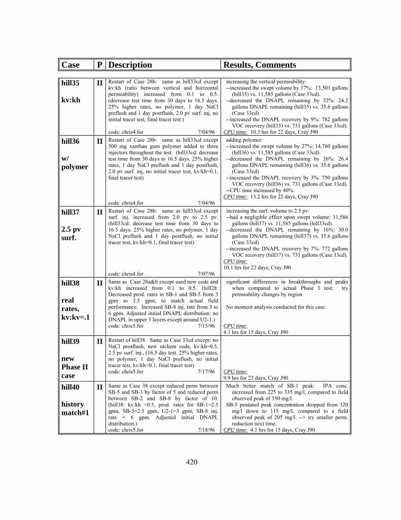
Case P Description Results, Comments
420
hill35 kv:kh
II Restart of Case 28b: same as hill33cd except kv:kh (ratio between vertical and horizontal permeability) increased from 0.1 to 0.5. (decrease test time from 30 days to 16.5 days. 25% higher rates, no polymer, 1 day NaCl preflush and 1 day postflush, 2.0 pv surf. inj, no initial tracer test, final tracer test.) code: chris4.for 7/04/96
increasing the vertical permeability: --increased the swept volume by 17%: 13,501 gallons
(hill35) vs. 11,585 gallons (Case 33cd). --decreased the DNAPL remaining by 32%: 24.2
gallons DNAPL remaining (hill35) vs. 35.6 gallons (Case 33cd)
--increased the DNAPL recovery by 9%: 782 gallons VOC recovery (hill35) vs. 731 gallons (Case 33cd).
CPU time: 10.3 hrs for 22 days, Cray J90
hill36 w/ polymer
II Restart of Case 28b: same as hill33cd except 500 mg xanthan gum polymer added to three injectors throughout the test. (hill33cd: decrease test time from 30 days to 16.5 days. 25% higher rates, 1 day NaCl preflush and 1 day postflush, 2.0 pv surf. inj, no initial tracer test, kv/kh=0.1, final tracer test) code: chris4.for 7/04/96
adding polymer: --increased the swept volume by 27%: 14,760 gallons
(hill36) vs. 11,585 gallons (Case 33cd). --decreased the DNAPL remaining by 26%: 26.4
gallons DNAPL remaining (hill36) vs. 35.6 gallons (Case 33cd)
--increased the DNAPL recovery by 3%: 750 gallons VOC recovery (hill36) vs. 731 gallons (Case 33cd).
--CPU time increased by 40%. CPU time: 13.2 hrs for 22 days, Cray J90
hill37 2.5 pv surf.
II Restart of Case 28b: same as hill33cd except surf. inj. increased from 2.0 pv to 2.5 pv. (hill33cd: decrease test time from 30 days to 16.5 days. 25% higher rates, no polymer, 1 day NaCl preflush and 1 day postflush, no initial tracer test, kv/kh=0.1, final tracer test) code: chris4.for 7/07/96
increasing the surf. volume to 2.5 pv: --had a negligible effect upon swept volume: 11,586
gallons (hill37) vs. 11,585 gallons (hill33cd). --decreased the DNAPL remaining by 16%: 30.0
gallons DNAPL remaining (hill37) vs. 35.6 gallons (Case 33cd)
--increased the DNAPL recovery by 7%: 772 gallons VOC recovery (hill37) vs. 731 gallons (Case 33cd).
CPU time: 10.1 hrs for 22 days, Cray J90
hill38 real rates, kv:kv=.1
II Same as Case 28a&b except used new code and kv:kh increased from 0.1 to 0.5. (hill28: Decreased prod. rates in SB-1 and SB-5 from 3 gpm to 2.5 gpm, to match actual field performance. Increased SB-8 inj. rate from 3 to 6 gpm. Adjusted initial DNAPL distribution: no DNAPL in upper 3 layers except around U2-1.) code: chris5.for 7/15/96
significant differences in breakthroughs and peaks when compared to actual Phase I test: try permeability changes by region
No moment analysis conducted for this case.
CPU time: 4.1 hrs for 15 days, Cray J90
hill39 new Phase II case
II Restart of hill38. Same as Case 33cd except: no NaCl postflush, new utchem code, kv:kh=0.5, 2.5 pv surf. inj., (16.5 day test. 25% higher rates, no polymer, 1 day NaCl preflush, no initial tracer test, kv/kh=0.1, final tracer test) code: chris5.for 7/17/96
CPU time: 9.9 hrs for 23 days, Cray J90
hill40 history match#1
II Same as Case 38 except reduced perm between SB-5 and SB-3 by factor of 5 and reduced perm between SB-2 and SB-8 by factor of 10. (hill38: kv:kh =0.5, prod. rates for SB-1=2.5 gpm, SB-5=2.5 gpm, U2-1=3 gpm, SB-8 inj. rate = 6 gpm. Adjusted initial DNAPL distribution.) code: chris5.for 7/18/96
Much better match of SB-1 peak: IPA conc. increased from 225 to 335 mg/l, compared to field observed peak of 350 mg/l.
SB-5 pentanol peak concentration dropped from 320 mg/l down to 115 mg/l, compared to a field observed peak of 205 mg/l. --> try smaller perm. reduction next time.
CPU time: 4.1 hrs for 15 days, Cray J90

Case P Description Results, Comments
421
hill41 history match#2
II Same as Case 38 except reduced perm between SB-5 and SB-3 by factor of 2 and reduced perm between SB-2 and SB-8 by factor of 10. (hill38: kv:kh =0.5, prod. rates for SB-1=2.5 gpm, SB-5=2.5 gpm, U2-1=3 gpm, SB-8 inj. rate=6 gpm. Adjusted initial DNAPL distribution.) code: chris5.for 7/19/96
SB-1 peak: IPA conc. increased from 225 to 300 mg/l, compared to field observed peak of 350 mg/l.
SB-5 pentanol peak concentration dropped from 320 mg/l down to 175 mg/l, compared to a field observed peak of 205 mg/l.
CPU time: 4.2 hrs for 15 days, Cray J90
hill42 fhistory match#3
II Same as Case 38 except reduced perm between SB-5 and SB-3 by factor of 5 in bottom 3 layers and reduced perm between SB-2 and SB-8 by factor of 10 and reduced perm between SB-3 and U2-1 by factor of 2. (hill38: kv:kh =0.5, prod. rates for SB-1=2.5 gpm, SB-5=2.5 gpm, U2-1=3 gpm, SB-8 inj. rate=6 gpm. Adjusted initial DNAPL distribution.) code: chris5.for 7/19/96
CPU time: 4.1 hrs for 15 days, Cray J90
hill43a repeat cray case on brazos
II Same as Case 42 except had to switch from cray to brazos (DEC-3000/500, 224 MB) code: chris5.for 7/20/96
switching from CRAY to brazos increased CPU execution time by an order of magnitude from 4.1 hours to 41.5 hours.
CPU time: 41.5. hrs for 15 days, (brazos): 10 times Cray CPU
hill43b repeat cray case on seaboard
II Same as Case 42 except switched from cray to seaboard (DEC-3000/610, 128 MB) code: chris5.for 7/20/96
switching from CRAY to seaboard increased CPU execution time by factor of 4.3: from 4.1 hours to 17.7 hours.
CPU time: 17.7. hrs for 15 days, Seaboard DEC-4000/610, 128 MB: 4.3 times Cray CPU
hill44a final history match #4
II Same as Case 43 except reduced perm between SB-2 and SB-8 by factor of 20. (hill43: hill38 plus reduced perm between SB-5 and SB-3 by factor of 5 in bottom 3 layers and reduced perm between SB-2 and SB-8 by factor of 10 and reduced perm between SB-3 and U2-1 by factor of 2. kv:kh =0.5, prod. rates for SB-1=2.5 gpm, SB-5=2.5 gpm, U2-1=3 gpm, SB-8 inj. rate=6 gpm. Adjusted initial DNAPL distribution.) code: chris5.for 7/21/96
Moment Analysis: 690 gal DNAPL contacted, much higher than 516 gal of field Phase I. Also higher than hill28, because kv:kh increased from 0.10 to 0.50, thereby increasing the sweep of layers above the completed layers?
switching from CRAY to seaboard increased CPU execution time by factor of 4.3: from 4.1 hours to 17.7 hours.
CPU time: 17.7. hrs for 15 days, Seaboard DEC-4000/610, 128 MB
hill44b pluto
II Repeat hill44a, except on CRAY code: chris5.for 7/21/96
CPU time: 4.2. hrs for 15 days, Cray-J90
hill45a Phase II w/ Phase I HM
II Restart of Seaboard Case 44a, (history matched Phase I w/ adjusted rates): Surfactant Flooding Segment (kv:kh=0.5, 2.5 pv surf. inj., (16.5 day test. 25% higher rates, no polymer, 1 day NaCl preflush, no initial tracer test, final tracer test) Adjusted initial DNAPL distribution.) code: chris5.for 7/21/96
Run on CRAY, using restart from Seaboard 16.5 day test, no initial tracer test
CPU time: 5.1. hrs for 10 days, Cray J90 ($92)
hill45b tracer test
II Restart of Seaboard Phase I Case 45a: Phase II Final Tracer test & extraction only segments. code: chris5.for 7/21/96
Run on CRAY, using restart from Seaboard:: error in C13 component in history files: increased from 0.43x10⁻² to 0.16x10+14 at 203.9 days -- try rerunning hilll44a on CRAY to use as restart (rather than switching machines in middle of run
CPU time: 3.7 hrs for 12 days, Cray J90 ($67)

Case P Description Results, Comments
422
hill45c surf. flood on pluto
II Restart of Cray Case 44a, (history matched Phase I w/ adjusted rate) Surfactant Flooding Segment (kv:kh=0.5, 2.5 pv surf. inj., (16.5 day test. 25% higher rates, no polymer, 1 day NaCl preflush, no initial tracer test, final tracer test) Adjusted initial DNAPL distribution.) code: chris5.for 7/22/96
Run on CRAY, using restart from Cray: still have problems with C13 component -- switch to chris4.for code
CPU time: 4.9 hrs for 10 days, Cray J90 ($89)
hill45d old code
II Restart of Seaboard Phase I Case 44a: 4.7 day test run code: chris4..for 7/21/96
Switch from chris5.for to chris4.for: Run on CRAY, using restart from Seaboard: looks ok
4.7 day run, Cray J90 ($100)
hill45e old code
II Restart of Seaboard Phase I Case 45d: code: chris4..for 7/21/96
finish 20 day test. 15.3 days run, Cray J90
hill46 less DNAPL
II Same as Case 44 Phase I except: (1) decrease DNAPL in layer 4 from 0.20 to 0.10 to reduce DNAPL contacted from the 690 gallons in hill44 initial tracer test, (2) switch back to chris4 code until problems with heptanol conc. resolved code: chris5.for 7/30/96
11.5 days, Seaboard DEC-4000/610, 128 MB
hill47 initial tracer test
II New Phase II case, restart of hill46: Same as Case 45 except: (1) reduced DNAPL, (2) chris4.for code, (3) add initial tracer test back into Phase II, and (4) remove 2,4 dimethyl-3-pentanol tracer from final tracer test (too costly) code: chris5.for 7/30/96
24 days, Seaboard DEC-4000/610, 128 MB
Note: All CPU times are for 1996 hardware and software. Computer run times in
2004 are substantially lower, due to enhancements in UTCHEM and hardware
improvements. For example, in 2004 a 22.4 day Hill AFB Phase II case required only
around 1.6 cpu hrs on a 2.4GHz Pentium PC (Delshad, 2004), in contrast to 9.9 cpu hrs on
a Cray in 1996 (Case 39).

423
NOMENCLATURE, ACRONYMS, AND NOTES ON CONVERSION OF UNITS
NOMENCLATURE
Cs = concentration of electrolytes; salinity, mg/l or meq/ml
selC = effective lower salinity; the lowest electrolyte concentration at which a Winsor type III system occurs; defines the boundary or transition between the Winsor type I (two phase, excess oil phase) and Winsor type III (three phase) system, mg/l or meq/ml
seuC = effective upper salinity; the highest electrolyte concentration at which a Winsor type III system occurs; defines the boundary or transition between the Winsor type III (three phase) system and the Winsor type II (two phase, excess water phase) system, mg/l or meq/ml
C*s or soptC = optimal salinity (electrolyte concentration) of the solution,
mg/l or meq/ml
23C = concentration of contaminant (component 2) in the microemulsion phase (phase 3), on a volumetric basis, [L3 /L3].
33
23
CC
= solubility ratio, concentration of contaminant in the
microemulsion divided by concentration of surfactant in the microemulsion
max3C = the maximum concentration of surfactant (component 3) in the microemulsion phase (phase 3), at a particular salinity, on a volumetric basis [L3 /L3]; represents the height of the binodal curve dividing the single phase and multi-phase regions of a ternary phase diagram

424
0max3C = height of the binodal curve at zero salinity (UTCHEM phase behavior model tuning parameter)
1max3C = height of the binodal curve at optimal salinity (UTCHEM phase behavior model tuning parameter)
2max3C = height of the binodal curve at double the optimal salinity (UTCHEM phase behavior model tuning parameter)
g = gravity
K = hydraulic conductivity; typical units of ft/d, gal/d/ft2, m/s, [L/T]
k = permeability, typical units of Darcy, m2, [L2]
rwk = relative permeability to water
totm = total mass of the mixture, mg, [m]
NC = capillary number; the ratio of viscous and capillary forces
NCc = critical capillary number; the minimum capillary number that must be reach for the residual (oil or DNAPL) saturation to begin to decrease, at which ‘mobilization’ of this freed residual phase may occur.
NB = Bond number; the ratio of gravity (or buoyancy) and capillary forces
NT = trapping number; combined Bond and capillary number; determines degree of ‘trapping’ or ‘mobilization’ of a residual saturation of a phase
n = porosity; pore volume divided by bulk volume; also referred to in petroleum literature as “φ ”
U = upper surface of the fluid in the pipette (air liquid interface), ml
IFi = initial level of the interface between the contaminant and the injection solution (before mixing), ml

425
IFwm = level of the interface between the upper aqueous phase and the middle-phase microemulsion, ml
IFmo = level of the interface between the middle-phase microemulsion and the lower oleic phase (DNAPL), ml
S1 = saturation, volume of phase 1 divided by total pore volume
Vinj = volume of injected surfactant solution, ml
Vo = volume of DNAPL (oleic phase), ml
Vom = volume of contaminant within the microemulsion, ml
Vw = volume of aqueous phase (water phase), ml
Vm = volume of microemulsion phase, ml
Vsm = volume of surfactant within the microemulsion, ml
Vsi = volume of surfactant initially added to the pipette, ml
L = lower level of fluid in the pipette (bottom of the pipette), ml
aρ = density of alcohol; typical units of g/cc, [M/L3]
totρ = total density of the mixture; typical units of g/cc, [M/L3]
wρ = density of water; typical units of g/cc, [M/L3]
wµ viscosity of water; typical units of cp (centipoise)
φ = porosity; pore volume divided by bulk volume; also referred to in environmental literature as “n”
SUBSCRIPTS:

426
o = oil phase or LNAPL or DNAPL
m = microemulsion phase
s = surfactant or salinity
a = alcohol
n = NAPL
i = initial conditions
inj = injected
w = water or aqueous phase
1 = the water component or the aqueous phase: if subscript consists of two digits, i.e. Cij, the first (i) refers to the component and the second (j) refers to the phase.
2 = the contaminant component or the DNAPL (or oil or oleic phase): if subscript consists of two digits, i.e. Cij, the first (i) refers to the component and the second (j) refers to the phase.
3 = the surfactant component or the microemulsion phase: if subscript consists of two digits, i.e. Cij, the first (i) refers to the component and the second (j) refers to the phase.

427
ACRONYMS AND DEFINITIONS
AFB Air Force Base
autochthonous indigenous or native, formed or originating in the place where found (bacteria)
CMC Critical Micellar Concentration; minimum surfactant concentration needed for surfactant monomers (single molecules) to form micelles, aggregates of surfactant molecules with a typically hollow spherical structure surrounding the dissolved component; the surfactant concentration must be greater than the CMC for microemulsion formation and the resultant greatly enhanced contaminant solubility
CMC carboxymethylcelulose, a polymer evaluated for mobility control in SEAR.
23DM2B 2,3Dimethyl-2-Butanol, alcohol tracer, Kow=24. (Setarge et al., 1999)
4M2P 4-Methyl-2-Penthanol, alcohol tracer, Kow=70. (Setarge et al., 1999)
EOR enhanced oil recovery; recovery of oil by means other than (and generally more complex than) primary depletion (“pump and treat”) or secondary recovery (waterflooding)
EWRE Environmental and Water Resources Engineering Program, within the Civil Engineering Department of the University of Texas, Austin.
HLB the hydrophile:lipophile balance, an empirical measure of surfactant hydrophobicity
HPCD Hydroxypropyl-β-cyclodextrin, glucose-based surfactant. (Boving et al., 1999)
IFT interfacial tension
IPA 2-propanol; isopropanol; isopropyl alcohol

428
MA brand name for a surfactant, sodium dihexyl sulfosuccinate; also referred to as MA-80 (shipped as a mixture of 80% active surfactant with the remaining 20% consisting of IPA and water)
MCD methyl-β-cyclodextrin, glucose-based surfactant. (Boving et al., 1999)
MCL Maximum Concentration Limit, safe drinking water standard, set by EPA
OU2 Operable Unit #2
SRS Source Recovery System, extraction wells (which extract DNAPL and contaminant dissolved in water) and surface treatment plant at Hill AFB OU2, operated by Radian
UT The University of Texas, at Austin
NOTES ON CONVERSION OF UNITS:
* 9 gpm = 13,000 gpd = 2.0 m3/s = 2000 l/s = 1700 ft3/d = 310 bbl/d
1 darcy = 1x10⁻⁵ m/s = 1 2mµ = 2.8 ft/day

429
REFERENCES
Abou-Nemeh, I., S. Majumdar, A. Saraf, K.K. Sirkar, L.M. Vane, F.R. Alvarez, and L. Hitchens: Demonstration of pilot-scale pervaporation systems for volatile organic compound removal from a surfactant enhanced aquifer remediation fluid II: Hollow fiber membrane modules, Environmental Progress, 20(1), 64-73, April, 2001.
Abriola, L.M., T.J. Dekker, and K.D. Pennell: Surfactant Enhanced Solubilization of Residual Dodecane in Soil Columns: 2. Mathematical Modeling, Environmental Science & Technology, 1993.
Abriola, L.M.: Modeling Multiphase Migration of Organic Chemicals in Groundwater Systems - A Review and Assessment, Environmental Health Perspectives, 83, 117-143, 1989.
Abriola, Linda M., Wendy E Condit, and Mathew A. Cowell: Influence of soil texture on rate-limited micellar solubilization, Journal of Environmental Engineering, 39-46, January 2000.
Annable, M.D., J.W. Jawitz, P.S.C. Rao, D.P. Dai, H. Kim, and A.L. Wood: Field evaluation of interfacial and partitioning tracers for characterization of effective NAPL-water contact areas, Ground Water, 36(3), 495-502, May-June 1998.
Annable, M.D., J.W. Jawitz, R.D. Rhue, P.S.C. Rao: Design of Surfactant/Cosolvent Flushing for Efficient NAPL Extraction using Results from a Cosolvent Flood, American Chemical Society, Emerging Technologies in Hazardous Waste Management VIII, Birmingham, September 9-11, 1996.
Annable, Michael D., P.S.C. Rao, Kirk Hatfield, Wendy D. Graham, A.L. Wood, and C.G. Enfield: Partitioning Tracers for Measuring Residual NAPL: Field Scale Test Results, Journal of Environmental Engineering, 498-503, June 1998.
Aziz, K., and A. Settari: Petroleum Reservoir Simulation, Applied Science Publishers Ltd., London, 1979.
Baran J.R. Jr., G.A. Pope, W.H. Wade, and V. Weerasooriya: “Microemulsion Formation with Chlorinated Hydrocarbons of Differing Polarity,” Environmental Science and Technology, 28 (7), 1361, 1994.

430
Baran, Jr., J.R., G.A. Pope, C. Schultz, W.H. Wade, V. Weerasooriya, and A. Yapa:. "Toxic Spill Remediation of Chlorinated Hydrocarbons via Microemulsion Formation," Surfactants in Solution, A.K. Chattopadhyay and K.L. Mittal (eds.), Marcel Dekker, Inc., New York, August, 1996.
Baran, Jr., J.R., and G.A. Pope: An overview of surfactant enhanced aquifer remediation, Progr. Colloid Polym. Sci, 109, 74-84, 1998.
Bear, J.: Hydraulics of Groundwater, McGraw-Hill, Inc., New York, 1979.
Bettahar, Mehdi, Gerhard Schafer, and Marc Baviere: Optimized surfactant formulation for the remediation of diesel oil polluted sandy aquifers, Environmental Science and Technology, 33(8), 1269-1273, Apr, 1999.
Bettahar, Mehdi, Jean Ducreux, Van Dorpe Schafer, and Francois Gerhard: : Surfactant enhanced in situ remediation of LNAPL contaminated aquifers: Large scale studies on a controlled experimental site, Transport in Porous Media, 37(3), 255-276, 1999.
Bhuyan, D., G.A. Pope, and L.W. Lake: Mathematical Modeling of High-pH Chemical Flooding, SPE Reservoir Engineering, 5(2), 213-220, 1990.
Bourell, M. and R.S. Schechter: Microemulsions and Related Systems, Marcel Dekker, Inc., 1988.
Boving, Thomas B., Xiaojiang Wang, and Mark L Brusseau: Cyclodextrin-enhanced solubilization and removal of residual-phase chlorinated solvents from porous media, Environmental Science and Technology, 33(5), 764-770 Mar 1, 1999.
Broholm, L., J.A. Cherry, and S. Feenstra: Dissolution of Heterogeneously Distributed Solvents Residuals, Subsurface Restoration Conference, Third International Conference on Ground Water Quality Research, Dallas, June 21-24, 1992.
Brooks, R.H. and A.T. Corey: Properties of Porous Media Affecting Fluid Flow, J. Irrig. Drain. Div., 6, 61-88, 1966.
Brown, C.L., G.A. Pope, L.M. Abriola, and K. Sepehrnoori: “Simulation of Surfactant-Enhanced Aquifer Remediation,” Water Resources Research, 30 (11) 2959-2977, 1994.
Brown, C.L., M. Delshad, V. Dwarakanath, D.C. McKinney, and G.A. Pope: Design of a field-scale surfactant enhanced remediation of a DNAPL contaminated

431
aquifer, I&EC Special Symposium, American Chemical Society, Birmingham, Sept 9-12, 1996.
Brown, C.L., M. Delshad, V. Dwarakanath, D.C. McKinney, G.A. Pope: “Design of a Field-Scale Surfactant Enhanced Remediation of a DNAPL Contaminated Aquifer,” Proceedings of the I&EC Special Symposium, ACS, Birmingham, Alabama, September, 1996.
Brown, C.L., M. Delshad, V. Dwarakanath, R.E. Jackson, J.T. Londergan, H.W. Meinardus, D.C. McKinney, T. Oolman, G.A. Pope, W.H. Wade: “Demonstration of Surfactant Flooding of an Alluvial Aquifer Contaminated with DNAPL,” Proceedings of the 213th American Chemical Society National Meeting, Special Symposium on Field Testing of Innovative Subsurface Remediation Technologies, San Francisco, April 13-17th, 1999.
Brown, C.L: “Simulation of Surfactant-Enhanced Remediation of Aquifers Contaminated by Dense Nonaqueous Phase Liquids,” M.S. Thesis, U. of Texas, Austin, 1993.
Brusseau, Mark L., Nicole T. Nelson, Mart Oostrom, Zhihui Zhang, Gwynn R. Johnson, and Tom W. Wietsma :Influence of heterogeneity and sampling method on aqueous concentrations associated with NAPL dissolution, Environmental Science and Technology, 34(17), 3657-3664, 2000.
Butler, Elizabeth C., and Kim F. Hayes: Micellar solubilization of nonaqueous phase liquid contaminants by nonionic surfactant mixtures: effects of sorption, partitioning and mixing, Water Research, 32(5), 1345-1354, May, 1998.
Cain, R. Brent, Gwynn R. Johnson, John E. McCray, William J. Blanford, and Mark L. Brusseau: Partitioning tracer tests for evaluating remediation performance, Ground Water, 38(5), 752-761, Sep-Oct 2000.
Carvalho, Moises N., Thomas C. Harmon, and Birgitte K. Ahring: Physico-chemically enhanced bioremediation of PAH-contaminated soil, Remediation of Chlorinated and Recalcitrant Compounds--2002, Proceedings of the Third International Conference on Remediation of Chlorinated and Recalcitrant Compounds, A.R. Gavaskar and A.S.C. Chen (Eds.), Battelle Press, Monterey, CA, Paper 2B-05, 2002
Carvalho, Moises N., Thomas C., Harmon, and Birgitte K. Ahring: Performance of a aerosol-surfactant enhanced air sparging: laboratory results, Remediation of Chlorinated and Recalcitrant Compounds--2002, Proceedings of the Third International Conference on Remediation of Chlorinated and Recalcitrant

432
Compounds, A.R. Gavaskar and A.S.C. Chen (Eds.), Battelle Press, Monterey, CA, Paper 2E-07, 8 pp., 2002
Chen, L., and R.C. Knox: Using vertical circulation wells for partitioning tracer tests and remediation of DNAPLs, Ground Water Monitoring and Remediation, 161-168, Summer 1997.
Cheng, H., D.A. Sabatini, and T.C.G. Kibbey: Solvent extraction for separating micellar-solubilized contaminants and anionic surfactants, Environmental Science and Technology, 35(14), 2995-3000, Jul 15, 2001.
Chevalier, Lizette R., Susan J. Masten, Roger B. Wallace, and David C. Wiggert: Experimental investigation of surfactant-enhanced dissolution of residual NAPL in saturated soil, Ground Water Monitoring & Remediation, 17(4), 89-98, Fall, 1997.
Conrad, S.H., R.J. Glass, and W.J. Peplinski: Bench-scale visualization of DNAPL remediation processes in analog heterogeneous aquifers: surfactant floods and in situ oxidation using permanganate, Journal of Contaminant Hydrology, 58(1-2), 13-49, September, 2002.
Core Laboratories, Soil Analysis Test Program, File Number DAL-95276, Final Report prepared by Core Laboratories, Inc., Carrolton, Texas, for INTERA, Inc., Austin, Texas, January 11, 1996.
Cowell, Matthew A., Tohren C.G. Kibbey, Julie B. Zimmerman, and Kim F. Hayes: Partitioning of ethoxylated nonionic surfactants in water/NAPL systems: effects of surfactant and NAPL properties, Environmental Science and Technology, 34(8), 1583-1588, Apr, 2000.
Datta Gupta, A., G.A. Pope, K. Sepehrnoori, and R.L. Thrasher: A Symmetric, Positive Definite Formulation of a Three-Dimensional Micellar/Polymer Simulator, SPE Reservoir Engineering, 1(6), 622-632, 1986.
Datta Gupta, A., L. W. Lake, G.A. Pope, K. Sepehrnoori, and M. J. King: High Resolution Monotonic Schemes for Reservoir Fluid Flow Simulation, In Situ, 15(3), 289-317, 1991.
de Blanc, P.C., D.C. McKinney, G.E. Speitel, Jr.: UTCHEM: A multiphase flow and Biodegradation model, Proceedings - SPE/EPA Exploration and Production Environmental Conference, Austin, SPE 52734, 1999.
Deeds, Neil E., Gary A. Pope, and Daene C. McKinney: Vadose zone characterization at a contaminated field site using partitioning interwell

433
tracer technology, Environmental Science and Technology, 33, 2745-2751, 1999.
Dekker, Timothy J, and Linda M. Abriola: Influence of field-scale heterogeneity on the surfactant-enhanced remediation of entrapped nonaqueous phase liquids, Journal of Contaminant Hydrology, 42(2), 219-251, Mar, 2000.
Delshad, Mohammad: Trapping of Micellar Fluids in Berea Sandstone, Ph.D. dissertation, The University of Texas, Austin, 1990.
Delshad, Mojdeh: A Study of the Transport of Micellar Fluids in Porous Media, Ph.D. dissertation, The University of Texas, Austin, 1986.
Delshad, M., G. A. Pope, and K. Sepehrnoori: A Compositional Simulator for Modeling Surfactant Enhanced Aquifer Remediation, 1: Formulation, Journal of Cont. Hydrology, 23, 303-327, 1996
Delshad, M., Pope, G. A., Yeh, L., and Holzmer, F. J.: Design of the Surfactant Flood at Camp Lejeune, Second International Conference on Remediation of Chlorinated and Recalcitrant Compounds, Monterey, California, May 22-25, 2000.
Delshad, Mojdeh, personal communication, email to the author, 2004.
Deshpande, S., L. Wesson, D. Wade, D.A. Sabatini, and J.H. Harwell: DOWFAX surfactant components for enhancing contaminant solubilization, Water Resources, 34(3), 1030-1036, 2000.
Dotelli, Giovanni, Allessandro Bevilacqua, Marinella Levi, Thomas P. Lockhart, and Steven L. Bryant: Factors influencing SEAR process efficiency, Remediation of Chlorinated and Recalcitrant Compounds--2002, Proceedings of the Third International Conference on Remediation of Chlorinated and Recalcitrant Compounds, A.R. Gavaskar and A.S.C. Chen (Eds.), Battelle Press, Monterey, CA, Paper 2C-31, 2002.
Duffield, A.R., R.S. Ramamurthy, and J.R. Campanelli: Surfactant enhanced mobilization of mineral oil within porous media, Water, Air, and Soil Pollution, 143(1-4), 111-122, February, 2003.
Dwarakanath, V. “Characterization and Remediation of Aquifers Contaminated by Nonaqueous Phase Liquids Using Partitioning Tracers and Surfactants.,” Ph.D. dissertation, U. of Texas, Austin, 1997.

434
Dwarakanath, Varadarajan, and Gary A. Pope: New approach for estimating alcohol partition coefficients between nonaqueous phase liquids and water, Environmental Science and Technology, 32, 1662-1666, 1998.
Dwarakanath, V., K. Kostarelos, Gary A. Pope, Doug Shotts, and William H. Wade: Anionic surfactant remediation of soil columns contaminated by nonaqueous phase liquids, Journal of Contaminant Hydrology, 38, 465-488, 1999.
Dwarakanath, Varadarajan, Neil E. Deeds, and Gary A. Pope: Analysis of partitioning interwell tracer tests, Environmental Science and Technology, 33, 3829-3836, 1999.
Dwarakanath, V., Britton, L. N., Jayanti. S., Ooi, K., Pope, G. A., and Weerasooriya, V., “Thermally Enhanced Surfactant Remediation,” Proceedings of the Seventh Annual International Petroleum Environmental Conference, Albuquerque, 2000.
Dwarakanath, V. and Pope, G. A.: Surfactant Phase Behavior with Field Degreasing Solvent, Environmental Science and Technology, 34(22), 4842-4848, 2000.
Dwarakanath, V., Jackson, R. E., and Pope, G. A.: Influence of Wettability on the Recovery of NAPLs from Alluvium, Environmental Science and Technology, 36(2), 227-231, 2002.
Dykstra, H., and R.L. Parsons: The Prediction of Oil Recovery by Water Flood, Secondary Recovery of Oil in the United States, 2nd ed., API, 202-222, 1950.
Elliott, B. P.: Laboratory Evaluation of the Neutral Buoyancy Approach to Surfactant Remediation, Master’s Thesis, The University of Texas at Austin, August 1999.
Finkel, M., R. Liedl, and G. Teutsch: Modelling surfactant-enhanced remediation of polycyclic aromatic hydrocarbons, Environmental Modelling & Software, 14(2-3), 203-211, 1999.
Fiorenza, Staphanie, Clarence A. Miller, Carrol L. Obre, and C.Herb Ward, editors: NAPL Removal: Surfactants, Foams, and Microemulsions, AATDF Monograph, CRC Press LLC, Lewis Publishers, 552 pp., 2000.
Fountain, J.C., R.C. Starr, T.M. Middleton, M. Beikirch, C. Taylor, and D. Hodge: A Controlled Field Test of Surfactant-Enhanced Aquifer Remediation, Ground Water, 34(5), 910-916, Sep-Oct 1996.
435
Fountain, J.C.: Field Test of Surfactant Flooding: Mobility Control of Dense Non-aqueous Phase Liquids, Chapter 15 in Transport and Remediation of Subsurface Contaminants, D.A. Sabatini and R.C. Knox (eds.), American Chemical Society Symposium Series 491, ACS, Washington D.C., 1992.
Freeze, G.A., J.C. Fountain, G.A. Pope, R.E. Jackson, M. Jin, V. Dwarakanath, B. Rouse, and K. Sepehrnoori: Proceedings of the 207th ACS National Meeting, San Diego, CA 34(1), 674-677, 1994.
Frind, E.O., G.G. Matanga, and J.A. Cherry: The Dual Formulation of Flow for Contaminant Transport Modeling, 2. The Borden Aquifer, Water Resources Research, 21(2), 170-182, 1985.
Gelhar, L.W., A. Mantoglou, C. Welty, and K.R. Rehfeldt: A Review of Field-Scale Physical Solute Transport Processes in Saturated and Unsaturated Porous Media, EPRI EA-4190, Electric Power Research Institute, Tennessee Valley Authority, 1985.
Haley, J.L., B. Hanson, C. Enfield, and J. Glass: Evaluating the Effectiveness of Ground Water Extraction Systems, Ground Water Mon. Rev., 11(3), 119-124, 1991.
Hargis and Associates: "Summary of Interim Remedial Investigations, January 1987 to April 1989, U.S. Air Force Plant No. 4", Volume I: Text, Tables & Illustrations, July 19, 1989.
Harwell, Jeffrey H., David A. Sabatini, and R.C. Knox: Surfactants for ground water remediation, Colloids and Surfaces A: Physicochemical and Engineering Aspects, v 151, n 1-2, Jun, 1999, p 255-268 "
Hasegawa, Mark H., Bor-Jier Shiau, David A. Sabatini, Robert C. Knox, Jeffrey H. Harwell, Rafael Lago, and Laura Yeh: Surfactant-enhanced subsurface remediation of DNAPLs at the former naval air station Alameda, California, Remediation of Chlorinated and Recalcitrant Compounds--2000, Proceedings of the Second International Conference on Remediation of Chlorinated and Recalcitrant Compounds, Wickramanayake et al., (Eds.), Battelle Press, Monterey, CA, Paper C2-2, 8 pp., 2000
Henry, E.J., and J.E. Smith: The effect of surface-active solutes on water flow and contaminant transport in variably saturated porous media with capillary fringe effects, Journal of Contaminant Hydrology, 56, 247-270, 2002.
Hirasaki, G.J., C.A. Miller, R. Szafranski, D. Tanzil, J.B. Lawson, H. Meinardus, M. Jin, R.E. Jackson, G. Pope, and W.H. Wade: Field demonstration of the

436
surfactant/foam process for aquifer remediation, Proceedings - SPE Annual Technical Conference, San Antonio, SPE 39292, 1997.
Hirasaki, G.J., C.A. Miller, R. Szafranski, J.B. Lawson, and N. Akiya, Surfactant/foam process for aquifer remediation, Proceedings - SPE International Symposium on Oilfield Chemistry, 471-480, 1997.
Hitchens, L, L.M. Vane, and F.R. Alvarez: VOC removal from water and surfactant solutions by pervaporation: A pilot study, Separation and Purification Technology, 24(1-2), 67-84, Jun 1, 2001.
Holbert, Charles, Stacey R. Opp, Hans Meinardus, Minquan Jin, Jeff Silva, and Jon Ginn: Performance assessment of a surfactant-enhanced aquifer remediation application, Remediation of Chlorinated and Recalcitrant Compounds--2002, Proceedings of the Third International Conference on Remediation of Chlorinated and Recalcitrant Compounds, A.R. Gavaskar and A.S.C. Chen (Eds.), Battelle Press, Monterey, CA, 2002.
Huh, C.: “Interfacial Tensions and Solubilizing Ability of a Microemulsion Phase that Coexists with Oil and Brine”, J. Colloid Interface Sci., 71, 408-426, 1979.
Intera: "Application of the UTCHEM Simulator to DNAPL-site Characterization and Remediation", Report 12202-02, submitted to The Center for Petroleum and Geosystems Engineering, The University of Texas at Austin by INTERA Inc., December 1994.
Intera: "Phase I Work Plan: Demonstration of Surfactant-Ehnanced Aquifer Remediation of DNAPLs at Hill Air Force Base", 00-ALC/EMR, prepared for AFCEE, Air Force Center for Environmental Excellence, Report Number 120201-6, INTERA, A Duke Engineering & Services Company, Austin, Texas, March 8, 1996.
Jackson, R.E.; and V. Dwarakanath: Chlorinated degreasing solvents: physical-chemical properties affecting aquifer contamination and remediation. Ground Water Monitoring & Remediation, pp. 102-110, 1999.
Jackson, R. E.: DNAPL Source Remediation in Alluvial Geosystems, DNAPL Source Remediation Workshop, Dallas, TX, October 2001.
Jackson, R. E.: The Evolution of DNAPL Remediation Practice, ACS Symposium Series 837, Chlorinated Solvent and DNAPL Remediation Innovative Strategies for Subsurface Cleanup, Henry, S. M. and Warner, S. D., Editors, 2003.

437
Jackson, R.E.; V. Dwarakanath, H.W. Meinardus, C.M. Young: Mobility Control: How Injected Surfactants and Biostiumulants may be Forced Into Low-Permeability Units, Remediation, pp. 59-66, Summer 2003.
Jain, Vivek, and Avery H. Demond: Conductivity reduction due to emulsification during surfactant enhanced-aquifer remediation. 1. Emulsion transport, Environmental Science and Technology, 36(24), 5426-5433, Dec 15, 2002.
Jain, Vivek, and Avery H. Demond: Conductivity reduction due to emulsification during surfactant enhanced-aquifer remediation. 2. Formation of emulsion in situ, Environmental Science and Technology, 36(24), 5434-5440, Dec, 2002.
Jawitz, James W., Michael D. Annable, P. Suresh C. Rao, and R. Dean Rhue: Field Implementation of a Winsor Type I surfactant/alcohol mixture for in situ solubilization of a complex LNAPL as a single-phase microemulsion, Environmental Science And Technology, 32(4), 523-530, 1998.
Jawitz, James W., Michael D. Annable, P.S.C. Rao, and R. Dean Rhue: Field Implementation of a Winsor Type I surfactant/alcohol mixture for in situ solubilization of a complex LNAPL as a single-phase microemulsion, Environmental Science and Technology, 32(4), 523-530, 1998.
Jawitz, James W., Randall K. Sillan, Michael D. Annable, P. Suresh C. Rao, and Kevin Warner: In-Situ Alcohol Flushing of a DNAPL Source Zone at a Dry Cleaner Site, Environmental Science And Technology, 34(17), 3722-3729, 2000.
Jayanti, S.: Evaluation of New Surfactants and Tracers, Master’s Report, The University of Texas at Austin, August 2000.
Jayanti. S., Britton, L. N., Dwarakanath, V., and Pope, G. A.: Laboratory Evaluation of Custom-Designed Surfactants To Remediate NAPL Source Zones, Environmental Science and Technology, 36(24), 5491-5497, 2002.
Jayanti, S.: Modeling Tracers And Contaminant Flux In Heterogeneous Aquifers, Ph.D. Dissertation, The University of Texas at Austin, August 2003.
Ji, Wei, and Mark L. Brusseau: A general mathematical model for chemical-enhanced flushing of soil contaminated by organic compounds, Water Resources Research, 34(7), 1635-1648, July 1998.
Jin, M., G.W. Butler, R.E. Jackson, P.E. Mariner, J.F. Pickens, G.A. Pope, C.L. Brown, and D.C. McKinney: Sensitivity Models and Design Protocol for Partitioning Tracer Tests in Alluvial Aquifers, Ground Water, 35(6), 964-972, Nov-Dec 1997.

438
Jin, M., M. Delshad, V. Dwarakanath, D.C. McKinney, G.A. Pope, K. Sepehrnoori, C. Tilburg, and R.E. Jackson: Partitioning Tracer Test for Detection, Estimation and Performance Assessment of Subsurface Nonaqueous Phase Liquids, Water Resources Research 30(5) 1201-1211, 1995.
Jin, M., Jackson, R. E., and Pope, G. A.: The Interpretation and Error Analysis of PITT data, Treating Dense Nonaqueous-Phase Liquids, The Second International Conference on Remediation of Chlorinated and Recalcitrant Compounds, Wickramanayake, G. B., Gavaskar, A. R., and Gupta, N., eds., Batelle Press, 85-92, 2000.
Jin, M: A Study of Nonaqueous Phase Liquid Characterization and Surfactant Remediation, Ph.D. dissertation, U. of Texas, Austin, 1995.
John, W. Wynn, Gaobin Bao, William P. Johnson, and Thomas B. Stauffer: Sorption of nonionic surfactant oligomers to sediment and PCE DNAPL: Effects on PCE distribution between water and sediment, Environmental Science and Technology, 34(4), 672-679, Feb, 2000.
Johnson, Jonathan C., Sun Shaobai, and Peter R. Jaffe: Surfactant enhanced perchloroethylene dissolution in porous media: The effect on mass transfer coefficients, Environmental Science and Technology, 33(8), 1286-1292, 1999.
Kim, Ju-Young, Claude Cohen, Michael L. Shuler, and Leonard W. Lion: Use of amphiphilic polymer particles for in situ extraction of sorbed phenanthrene from a contaminated aquifer material, Environmental Science and Technology, 34(19), 4133-4139, Oct, 2000.
Knox, R.C., D.A., Sabatini, J.H. Harwell, R.E. Brown, C.C. West, F. Blaha, and C. Griffin: Surfactant remediation field demonstration using a vertical circulation well, Ground Water, 35(6), 948-953, Nov-Dec, 1997.
Ko, Seok-Oh, and Mark A. Schlautman: Partitioning of hydrophobic organic compounds to sorbed surfactants. 2. Model development/predictions for surfactant-enhanced remediation applications, Environmental Science and Technology, 32(18), 2776-2781, Sep 15, 1998.
Kostarelos, K. , G.A. Pope, B.A. Rouse, and G.M. Shook: New concept: the use of neutrally-buoyant microemulsions for DNAPL remediation, Journal of Contaminant Hydrology, 34(4), 383-397, Nov 15, 1998.
Krebs-Yuill, B., J.H. Harwell, D.A. Sabatini, and R.C. Knox: Economic considerations in surfactant-enhanced pump-and-treat remediation,

439
Surfactant-Enhanced Subsurface Remediation, American Chemical Society, Chapter 19, 265-278, 1995.
Kueper, B. H. and D. B. McWhorter: The Behavior of Dense, Nonaqueous Phase Liquids in Fractured Clay and Rock, Ground Water, 29(5), 716-728, 1991.
Kueper, B.H., D. Redman, R.C. Starr, S. Reitsma, and M. Mah: A Field Experiment to Study the Behavior of Tetrachloroethylene Below the Water Table: Spatial Distribution of Residual and Pooled DNAPL, Ground Water, 31(5), 756-766, 1993.
Kueper, B.H.: The Behavior of Dense, Non-Aqueous Phase Liquid Contaminants in Heterogeneous Porous Media, Ph.D. dissertation, The University of Waterloo, Ontario, 1989.
Lake, L.W.: Enhanced Oil Recovery, Prentice-Hall, Inc., New Jersey, 1989.
Lee, Dal-Heui, Robert D. Cody, Dong-Ju Kim, and Sangil Choi: Effect of soil texture on surfactant-based remediation of hydrophobic organic-contaminated soil, Environment International, 27(8), 681-688, 2002.
Leverett, M.C.: Flow of Oil-water Mixtures through Unconsolidated Sands, Trans., AIME, 132, 149-171, 1941.
Li, Zhaohui, Cari Willms, Pengfei Zhang, and Robert S. Bowman: Rate and pathway changes in PCE dechlorination by zero-valent iron in the presence of cationic surfactant, Remediation of Chlorinated and Recalcitrant Compounds--2002, Proceedings of the Third International Conference on Remediation of Chlorinated and Recalcitrant Compounds, A.R. Gavaskar and A.S.C. Chen (Eds.), Battelle Press, Monterey, CA, Paper 2C-35, 2002.
Liu, J., M. Delshad, G.A. Pope, and K. Sepehrnoori: Application of Higher-Order Flux-Limited Methods in Compositional Simulation, submitted to the Journal of Transport in Porous Media, November 1992.
Londergan, J.T., H.W. Meinardus, P.E. Mariner, R.E. Jackson, C.L., Brown, V. Dwarakanath, G.A. Pope, J.S. Ginn, and S. Taffinder: DNAPL removal from a heterogeneous alluvial aquifer by surfactant-enhanced aquifer remediation, Ground Water Monitoring and Remediation, 21(4), 57-67, 2001.
Lowe, Donald F., Carroll L. Oubre, and C. Herb Ward, editors: Surfactants and Cosolvents for NAPL Remediation, A Technology Practices Manual, AATDF Monograph, CRC Press LLC, Lewis Publishers, 412 pp., 2000.

440
MacFarlane, D.S., J.A. Cherry, R.W. Gilham, and E.A. Sudicky: Migration of Contaminants in Groundwater at a Landfill: A Case Study, 1. Groundwater flow and Plume Delineation, Journal of Hydrology, 63, 1-29, 1983.
Mackay, D.M. and J.A. Cherry, Groundwater Contamination: Pump and Treat Remediation, Environmental Science and Technology, 23(6), 630-636, 1989.
Mackay, D.M., D.L. Freyberg, P.V. Roberts, and J.A. Cherry: A Natural Gradient Experiment on Solute Transport in a Sand Aquifer, 1. Approach and Overview of Plume Movement, Water Resources Research, 22(13), 2017-2029, 1986.
Mariner, Paul E., Minquan Jin, and Richard E. Jackson: Chlorinated degreasing solvents: Physical-chemical properties affecting aquifer contamination and remediation, Ground Water Monitoring & Remediation, 122-129, Spring 1997.
Martel, K.E., R. Martel, R. Lefebvre, and P.J. Gelinas: Laboratory study of polymer solutions used for mobility control during in situ NAPL recovery, Ground Water Monitoring & Remediation, 18(3), 103-113, Summer, 1998.
Martel, Richard, Pierre J. Gelinas, and Laurent Saumure: Aquifer washing by micellar solutions: 3 Field test at the Thouin Sand Pit (L'Assomption, Quebec, Canada), JCH, 30, 33-48, 1998.
Mayer, A. S. and Miller, C. T.: The influence of mass transfer characteristics and porous media heterogeneity on nonaqueous phase dissolution, Water Resources Research, 32(6), 1551-1567, June 1996.
Mayer, Alex S., Lirong Zhong, and Gary A. Pope: Measurement of mass-transfer rates for surfactant-enhanced solubilization of nonaqueous phase liquids, Environmental Science and Technology, 33(17), 2965-2972, Sep, 1999.
McCray, John E., and Mark L. Brusseau: Cyclodextrin-Enhanced in Situ Flushing of Multiple-Component Immiscible Organic Liquid Contamination at the Field Scale: Mass Removal Effectiveness, Environmental Science & Technology, 32(9), 1285-1293, 1998.
Meinardus, H.W., V. Dwarakanath, J. Ewing, G.J. Hirasaki, R.E. Jackson, M. Jin, J.S. Ginn, J.T. Londergan, C.A. Miller, and G.A. Pope: Performance assessment of NAPL remediation in heterogeneous alluvium, Journal of Contaminant Hydrology, 54(3-4), 173-193, 2002.
441
Meinardus, H.W., Varadarajan Dwarakanath, John Ewing, Kimberly Gordon, George J. Hirasaki, Charles Holbert, and Jon Ginn: Full-scale field application of surfactant-foam process for aquifer remediation, Remediation of Chlorinated and Recalcitrant Compounds--2002, Proceedings of the Third International Conference on Remediation of Chlorinated and Recalcitrant Compounds, A.R. Gavaskar and A.S.C. Chen (Eds.), Battelle Press, Monterey, CA, 2002a.
Meinardus, H. W., Dwarakanath, V., Ewing, J., Gordon, K. D., Hirasaki, G. J., Holbert, C., and Ginn, J. S.: Full-scale field application of surfactant-foam process for aquifer remediation, Proceedings of the Third International Conference on Remediation of Chlorinated and Recalcitrant Compounds, Monterey, CA, May 20-23, 2002b.
Miller, Cass T., George Christakos, Paul T. Imhoff, John F. McBride, Joseph A. Pedit, and John A. Trangenstein: Multiphase flow and transport modeling in heterogeneous porous media: challenges and approaches, Advances in Water Resources, 21(2), 77-120, 1998.
Nash, J.H.: Field Studies of In-Situ Washing, U.S. Environmental Protection Agency, Cincinnati, OH, EPA/600/2-87/110, 1987.
National Research Council: Environmental Epidemiology, Volume I: Public Health and Hazardous Wastes, National Academy Press, Washington, D.C., 1991.
NFESC Technical Report TR-2206-ENV: Surfactant-Enhanced Aquifer Remediation (SEAR) Design Manual, Prepared for Naval Facilities Engineering Command, Washington, DC, April 2002.
Oolman, T., S. T. Godard, G. A. Pope, M. Jin, and K. Kirchner: “DNAPL Flow Behavior in a Contaminated Aquifer: Evaluation of Field Data.” GMWR, 125-137, Fall 1995.
Peng, Wei-Shyuan, Duane R. Hampton, Leonard F. Konikow, Kiran Kambham, and Jeffrey J. Benegar: Can contaminant transport models predict breakthrough?, Ground Water Monitoring and Remediation, 20(4), 104-113, Autumn, 2000.
Pennell, K.D., L.M. Abriola, and W.J. Weber, Jr.: Surfactant Enhanced Solubilization of Residual Dodecane in Soil Columns: 1. Experimental Investigation, Environmental Science and Technology, 1993a.
Pennell, K.D., M. Jin, L.M. Abriola, and G.A. Pope: Surfactant Enhanced Remediation of Soil Columns Contaminated by Residual Tetrachloroethylene, submitted to J. of Contaminant Hydrology, May, 1993b.

442
Pennell, Kurt D., Gary A. Pope, and Linda M. Abriola: Influence of Viscous and Buoyancy Forces on the Mobilization of Residual Tetrachloroethylene during Surfactant Flushing, Environmental Science and Technology, 30 (4), 1328-1335, 1996.
Pope, G.A. and M. Bavière: Basic Concepts in Enhanced Oil Recovery Processes, Critical Reports on Applied Chemistry, Volume 33, M. Bavière (ed.), Elsevier Science Publishing, London, 1991.
Pope, G.A. and R.C. Nelson: A Chemical Flooding Compositional Simulator, Society Petroleum Engineering Journal, 18(5), 339-354, 1978.
Pope, G.A., K. Sepehrnoori, M. Delshad, B. Rouse, V. Dwarakanath, M. Jin, A Abubakar, and M. Lim: "NAPL Partitioning Interwell Tracer Test in OU1 Test Cell at Hill Air Force Base, Utah", Final Report for Man Tech Environmental Research Service Corporation, October 12, 1994.
Pope, G.A., K. Sepehrnoori, M. Delshad, B. Rouse, V. Dwarakanath, M. Jin, A Abubakar, and M. Lim: "NAPL Partitioning Interwell Tracer Test in OU1 Test Cell at Hill Air Force Base, Utah", Final Report for Man Tech Environmental Research Service Corporation, October 12, 1994.
Pope, Gary A., Kamy Sepehrnoori, Mukul M. Sharma, Daene C. McKinney, Gerald E. Speitel Jr., and Richard E. Jackson: Three-dimensional NAPL fate and transport model, EPA Environmental Research Brief CR-821897, 1997.
Pope, Gary A., Kamy Sepehrnoori, Mojdeh Delshad, Bruce Rouse, Varadarajan Dwarakanath, Minquan Jin, Adil Abubakar, and Meng H. Lim: Final Report: NAPL Partitioning Interwell Tracer Test in OU1 Test Cell at Hill Air Force Base, Utah. University of Texas at Austin, 1994.
Pope, Gary A., Minquan Jin, Varadarajan Dwarakanath, Bruce Rouse, and Kamy Sepehrnoori: “Partitioning Tracer Tests to Characterize Organic Contaminants.” Proceedings of Second Tracer Workshop in Univ. of Texas at Austin, 1994
Pope, G. A. and Wade, W. H.: Lessons from Enhanced Oil Recovery Research for Surfactant-Enhanced Aquifer Remediation, in Surfactant-Enhanced Subsurface Remediation, Emerging Technologies, Sabatini, D. A., Knox, R. C., Harwell, J. H. (editors), ACS symposium series 594, American Chemical Society, Washington DC, 142-160, 1995.
Powers, S.E., C.O. Loureiro, L.M. Abriola, and W.J. Weber, Jr.: Theoretical Study of the Significance of Nonequilibrium Dissolution of Nonaqueous Phase

443
Liquids in Subsurface Systems, Water Resources Research, 27(4), 463-477, 1991.
Radian, “Results of the Surfactant Treatability Study for Operable Unit 2 Hill Air Force Base, “Utah, Draft. 1994b. RCN 279-104-08-10.
Radian: “Draft Site Health and Safety Plan for Source Removal System, Operable Unit 2, Hill Air Force Base, Utah,” prepared for 00-ALC/EMR Hill Air Force Base, Utah, June, 1993.
Radian: “Final Remedial Investigation for Operable Unit 2-Sites WP07 and SS21,” Prepared for Hill AFB, Utah. 1992.
Radian: “Work Plan: DNAPL Flow Characterizations in Aquifer Sands, Data Analysis Tasks, Operable Unit 2,” Hill Air Force Base, Utah. 1993.
Radian: Aquifer Data Evaluation Report, Operable Unit 2, Hill Air Force base, Utah. Radian, 1994a. RCN 279-100-26-41.
Ramsburg, C. Andrew, and Kurt D. Pennell: Density-modified displacement for DNAPL source zone remediation: Density conversion and recovery in heterogeneous aquifer cells, Environmental Science and Technology, 36(14), 3176-3187, Jul, 2002.
Ramsburg, C. Andrew, and Kurt D. Pennell: Density-modified displacement for dense nonaqueous-phase liquid source-zone remediation: Density conversion using a partitioning alcohol, Environmental Science and Technology, 36(9), 2082-2087, May 1, 2002.
Ramsburg, C. Andrew, Kurt D. Pennell, Tohren C.G. Kibbey, and Kim F. Hayes: Density-modified displacement of trichloroethene using partitioning alcohol and low interfacial tension surfactant floods, Remediation of Chlorinated and Recalcitrant Compounds--2002, Proceedings of the Third International Conference on Remediation of Chlorinated and Recalcitrant Compounds, A.R. Gavaskar and A.S.C. Chen (Eds.), Battelle Press, Monterey, CA, Paper 2C-29, 2002.
Ramsburg, C.A., and K.D. Pennell: Experimental and economic assessment of two surfactant formulations for source zone remediation at a former dry cleaning facility, Ground Water Monitoring and Remediation, 21(4), 68-82, 2001.
Rao, P. Suresh C., Michael D. Annable, and Heonki Kim: NAPL source zone characterization and remediation technology performance assessment: recent developments and applications of tracer techniques, Journal of Contaminant Hydrology, 45, 63-78, 2000.

444
Rothmel, R.K., R.W. Peters, E.S. Martin, and M.F. Deflaun: Surfactant foam/bioaugmentation technology for in situ treatment of TCE-DNAPLs, Environmental Science and Technology, 32(11), 1667-1675, Jun 1, 1998.
RUST Geotech, Inc.: "Air Force Plant 4 Remedial Investigation (RI) Report", September 1993.
Saad, N., G.A. Pope, and K. Sepehrnoori: Application of Higher-Order Methods in Compositional Simulation, SPE Reservoir Engineering, 5(4), 623-630, 1990.
Saad, N.: Field Scale Simulation of Chemical Flooding, Ph.D. dissertation, The University of Texas, Austin, 1989.
Saba, T., T.H. Illangasekare, and J. Ewing: Investigation of surfactant-enhanced dissolution of entrapped nonaqueous phase liquid chemicals in a two-dimensional groundwater flow field, Journal of Contaminant Hydrology, 51(1-2), 63-82, 2001.
Sabatini, D.A., R.C. Knox, J.H. Harwell, T. Soerens, L. Chen, R.E. Brown, and C.C. West: Design of a surfactant remediation field demonstration based on laboratory and modeling studies, Ground Water, 35(6), 954-963, Nov-Dec 1997.
Sabatini, David A., Jeffrey H. Harwell, Mark Hasegawa, and Robert Knox: Membrane processes and surfactant-enhanced subsurface remediation: Results of a field demonstration, Journal of Membrane Science, 151(1), 87-98, Dec 09, 1998.
Sabatini, David A., Robert C. Knox, Jeffrey H. Harwell, and Ben Wu: Integrated design of surfactant enhanced DNAPL remediation: efficient supersolubilization and gradient systems, JCH, 45, 99-121, 2000.
Saenton, S., T.H. Illangasekare, K. Soga, and T.A. Saba: Effects of source zone heterogeneity on surfactant-enhanced NAPL dissolution and resulting remediation end-points, Journal of Contaminant Hydrology, 59(1-2), 27-44, November, 2002.
Sahoo, D., Smith, J.A., T. E. Imbrigiotta, and H.M. McLellan,: Surfactant-enhanced remediation of a trichloroethene-contaminated aquifer. 2. Transport of TCE, Environmental Science and Technology, 32(11), 1686-1693, Jun 1, 1998.
Sale, Tom C., and David B. McWhorter: Steady state mass transfer from single-component dense nonaqueous phase liquids in uniform flow fields, Water Resources Research, 37(2), 393-404, February, 2001.
445
Santharam, S.K., L.E. Erickson, and L.T. Fan: Modelling the role of surfactant and biodegradation in the remediation of aquifers with non-aqueous phase contaminants, Journal of Hazardous Materials, 53(1-3), 115-139, May, 1997.
Schlumberger: Log Interpretation, Volume I - Principles. Schlumberger Limited Publishing, New York, 1972.
Setarge, B., J. Danzer, R. Klein, and P. Grathwohl: Partitioning and interfacial tracers to characterize non-aqueous phase liquids (NAPLs) in natural aquifer material, Physics and Chemistry of the Earth Part B: Hydrology, Oceans and Atmosphere, 24(6), 501-510, 1999.
Severin, Blaine, F., and Shannon Harris: Surfactant recovery in a novel three-phase soil washing system, Remediation of Chlorinated and Recalcitrant Compounds--2002, Proceedings of the Third International Conference on Remediation of Chlorinated and Recalcitrant Compounds, A.R. Gavaskar and A.S.C. Chen (Eds.), Battelle Press, Monterey, CA, Paper 2C-34, 2002.
Shook, G. Michael, Gary A. Pope, and K. Kostarelos: Prediction and minimization of vertical migration of DNAPLS using surfactant enhanced aquifer remediation at neutral buoyancy, Journal of Contaminant Hydrology, 34(4), 363-382 Nov 15, 1998.
Shook, G. Mike, K. Kostarelos, and G.A. Pope: Minimization of vertical migration of DNAPLs using surfactant enhanced aquifer remediation at neutral buoyancy, Proceedings - SPE Annual Technical Conference and Exhibition, Vol. Pi, Production Operations and Engineering/General, 931-939, 1997.
Shotts, D.R.: “Surfactant Remediation of Soils Contaminated with Chlorinated Solvents,” M.S. thesis, U. of Texas, Austin, 1996.
Silva, Jeff A.K., Paul E. Mariner, Hans W. Meinardus, and Jon S. Ginn: Monitoring partitioning tracer testing and surfactant flooding by in-line gas chromatography techniques, Ground Water Monitoring & Remediation, 23(1), 85-92, Winter 2003.
Skoog, D.A. and J.J. Leary: Principles of Instrumental Analysis. 4th ed., Saunders College Publishing, 1992.
Smith, James A., Dipak Sahoo, Heather M. McLellan, and Thomas E. Imbrigiotta: Surfactant-enhanced remediation of a trichloroethene-contaminated aquifer. 1. Transport of Triton X-100, Environmental Science and Technology, 31(12), 3565-3572, Dec, 1997.

446
Sudicky, E.A., J.A. Cherry, and E.O. Frind: Migration of Contaminants in Groundwater at a Landfill: A Case Study, 4. A Natural-Gradient Dispersion Test, Journal of Hydrology, 63, 81-108, 1983.
Sudicky, E.A.: A Natural Gradient Experiment on Solute Transport in a Sand Aquifer: Spatial Variability of Hydraulic Conductivity and Its Role in the Dispersion Process, Water Resources Research, 22(13), 2069-2082, 1986.
Sykes, J.B., S.B. Pahwa, R.B. Lantz, and D.S. Ward: Numerical Simulation of Flow and Contaminant Migration at an Extensively Monitored Landfill, Water Resources Research, 18(6), 1687-1704, 1982.
Szafranski, R., J.B. Lawson, G.J. Hirasaki, C. A. Miller: Improved Efficiency of Surfactant Remediation Processes Using Foam, American Chemical Society, Emerging Technologies in Hazardous Waste Management VIII, Birmingham, September 9-11, 1996.
TerraTek: DNAPL Flow Characterizations in Aquifer Sands, Hill Air Force Base, OU2, Report #TR94-45 TerraTek Inc., March 1994.
Texas Research Institute, Inc.: Test Results of Surfactant Enhanced Gasoline Recovery in a Large-Scale Model Aquifer, API Publication 4390, American Petroleum Institute, Washington, D.C., 1985.
Uchiyama, Hirotaka, Edgar Acosta, San Tran, David A. Sabatini, and Jeffrey A. Harwell: Supersolubilization in chlorinated hydrocarbon microemulsions: solubilization enhancement by lipophilic and hydrophilic linkers, Ind. Eng. Chem. Res., American Chemical Society, 39, 2704-2708, 2000.
van Genuchten, M.T.: A Closed-Form Equation for Predicting the Hydraulic Conductivity of Unsaturated Soils, Soil Sci. Soc. Am. J., 44, 892-898, 1980.
Verschueren, K.: Handbook of Environmental Data on Organic Chemicals, Van Nostrand Reinhold Company, Inc., New York, 1983.
Walker, R.C., C. Hofstee, J.H. Dane, and W.E. Hill: Surfactant enhanced removal of PCE in a partially saturated, stratified porous medium, Journal of Contaminant Hydrology, 34(1-2), 31-46, Oct 15, 1998.
West, C.C. and J.H. Harwell: Surfactants and Subsurface Remediation, Environmental Science Technology, 26(12), 2324-2330, 1992.
West, C.C.: Surfactant Enhanced Solubilization of Tetrachloroethylene and Degradation Products in Pump and Treat Remediation, Transport and

447
Remediation of Subsurface Contaminants, Chapter 12, American Chemical Society, 149-158, 1992.
Wilson, D.J. and A.N. Clarke: Soil Clean Up by In-Situ Surfactant Flushing: IV. A Two-Component Mathematical Model, Separation Science and Technology, 26(9), 1177-1194, 1991.
Wilson, D.J.: Soil Clean Up by In-situ Surfactant Flushing. 1. Mathematical Modeling, Separation Science and Technology, 24, 863-892, 1989.
Wilson, J.L. and S.H. Conrad: Is Physical Displacement of Residual Hydrocarbons a Realistic Possibility in Aquifer Restoration?, Proceedings of the NWWA Conference on Petroleum Hydrocarbons and Organic Chemicals in Ground Water, National Water Well Association, Dublin, OH, 274-298, 1984.
Wu, Wei-Jr, Delshad, M., Oolman, T. and Pope, G. A.: Remedial Options for Creosote Contaminated Sites, Ground Water Monitoring and Remediation, 78-86, Spring 2000.
Yang, A.P.: Stochastic Heterogeneity and Dispersion, Ph.D. dissertation, The University of Texas, Austin, 1990.
Yang, Jiangang, Xiang Liu, Tao Long, Gang Yu, Peng She, and Zheng Liu: Solubilization and biodegradation of phenanthrene in aqueous nonionic surfactant systems, Remediation of Chlorinated and Recalcitrant Compounds--2002, Proceedings of the Third International Conference on Remediation of Chlorinated and Recalcitrant Compounds, A.R. Gavaskar and A.S.C. Chen (Eds.), Battelle Press, Monterey, CA, Paper 2B-01, 2002
Yoon, S., I. Barman, A. Datta-Gupta, and G.A. Pope: In-situ characterization of residual NAPL distribution using streamline-based inversion of partitioning tracer tests, Proceedings - SPE/EPA Exploration and Production Environmental Conference, Austin, SPE 52729, 1999.
Young, C.M., R.E. Jackson, M. Jin, J.T. Londergan, P.E. Mariner, G.A. Pope, E.J. Anderson, and T. Houk: Characterization of a TCE DNAPL zone in alluvium by partitioning tracers, Ground Water Monitoring & Remediation, 19(1), 84-94, Winter, 1999.
Young, Carl M., Varadarajan Dwarakanath, Taimur Malik, Larry Milner, Joseph Chittet, Andreas Jazdanian, Nancy Huston, and Vinitha Weerasooriya: In situ remediation of coal tar-impacted soil by polymer-surfactant flooding, Remediation of Chlorinated and Recalcitrant Compounds--2002, Proceedings of the Third International Conference on Remediation of

448
Chlorinated and Recalcitrant Compounds, A.R. Gavaskar and A.S.C. Chen (Eds.), Battelle Press, Monterey, CA, Paper 2C-33, 8 pp., 2002
Zhong, Lirong, Alex S. Mayer, and Gary A. Pope: The effects of surfactant formulation on nonequilibrium NAPL solubilization, Journal of Contaminant Hydrology, 60(1-2), 55-75, January, 2003.
Zhou, Meifang, and R. Dean Rhue: Screening commercial surfactants suitable for remediating DNAPL source zones by solubilization, Environmental Science and Technology, 34(10), 1985-1990, 2000.
Zimmerman, Julie B., Tohren C.G. Kibbey, Matthew A. Cowell, and Kim F. Hayes: Partitioning of ethoxylated nonionic surfactants into nonaqueous-phase organic liquids: Influence on solubilization behavior, Environmental Science and Technology, 33(1), 169-176, Jan 1, 1999.

449
VITA
Chrissi Lynn Brown was born in Lindale, Texas on August 8, 1959, the
daughter of George Frank and Patricia Ann Brown. In 1982, upon graduating from
the University of Texas with a B.S. degree in petroleum engineering, she went to
work at ChevronTexaco as a reservoir engineer. In 1991, after nine years with
ChevronTexaco and assignments in Houston, Sumatra, London, and New Orleans,
Chrissi took a leave of absence and entered graduate school at the University of
Texas at Austin to pursue an M.S. in Petroleum Engineering, completed in 1993. In
1994 she was accepted into the Environmental and Water Resources Engineering
Program of the Civil Engineering Department at UT. After completing Ph.D. course
work and research, Chrissi returned to ChevronTexaco, working in California and
Kazakhstan, from 1997-2002. In 2002, Chrissi retired from ChevronTexaco and
returned to UT to complete the dissertation and Ph.D.
Permanent Address: 1314 Falcon Ledge, #115,
Austin, Texas, 78746, [email protected]
This dissertation was typed by the author.