copyright by angela kelechi eluwa 2015
TRANSCRIPT

Copyright
By
Angela Kelechi Eluwa
2015

The Thesis Committee for Angela Kelechi Eluwa
Certifies that this is the approved version of the following thesis:
Depositional Systems Analysis of the Lower Miocene Interval in Refugio
County, Western Gulf of Mexico Basin
APPROVED BY
SUPERVISING COMMITTEE:
David Mohrig, Supervisor
William L. Fisher, Co-Supervisor
Osareni C. Ogiesoba, Co-Supervisor

Depositional Systems Analysis of the Lower Miocene Interval in Refugio
County, Western Gulf of Mexico Basin
By
Angela Kelechi Eluwa, B.S.
Thesis
Presented to the Faculty of the Graduate School of
The University of Texas at Austin
in Partial Fulfillment
of the Requirements
for the Degree of
Master of Science in Energy and Earth Resources
The University of Texas at Austin
August 2015

Dedication
To my Dad and siblings.

v
Acknowledgements
It is with immense appreciation that I thank my supervisors. Despite their very
busy schedule, they always took the time to assist me. Dr. David Mohrig gave me
tireless support throughout the period of my thesis. His calm way of re-directing me,
whenever I got stuck had a great and positive impact on me to keep working. Dr. William
Fisher, who was also my academic advisor, provided immeasurable assistance throughout
my academic period. I would like to thank Dr. Christopher Ogiesoba for taking me as his
protégé; he provided the fundamentals and organization of my research.
This thesis was sponsored by the State of Texas Advanced Oil and Gas Resource
Recovery (STARR) group of the Bureau of Economic Geology at The University of
Texas at Austin. In particular, I would like to express my gratitude to Dr. William
Ambrose; he never hesitated to share his expertise whenever I found myself bound by the
complexities of this research. Thanks to T.C. Oil Company for the seismic data set and
also, thanks to T.C. Oil and IHS companies for the well log data.
I sincerely appreciate the technical assistance provided by Dallas Dunlap, David
Smith, and members of the Gulf of Mexico Basin Depositional Synthesis (GBDS)
research team – Dr. Jon Snedden and Jonathan Virdell. My smooth sail throughout my
graduate program was courtesy my graduate coordinator- Ms. Jessica Smith, thank you
very much for your readiness to provide necessary academic information.
To my family, especially my brother Dr. George Eluwa, I won’t be here without
your love and support. Your belief in me, strengthened my resolve to succeed. To my
first mentor, Dr. A.Y.B Anifowose, you laid the academic foundation on which I have
achieved this feat. Thank you.

vi
Abstract
Depositional Systems Analysis of the Lower Miocene Interval in Refugio
County, Western Gulf of Mexico Basin
Angela Kelechi Eluwa, M.S.E.E.R.
The University of Texas at Austin, 2015
Supervisor: David Mohrig
Co-supervisor: William L. Fisher
Co-supervisor: Osareni C. Ogiesoba
Definition of the environments within a depositional system provides useful
information about the possible depositional processes; and in turn helps predict the
amount and caliber of sediments transported to the basin. This research analyzes variance
attribute maps to identify the different environments of deposition within Refugio
County, Texas; this analysis also addresses the possible influence by the San Marcos
Arch on Lower Miocene deposition.
The study area is subsurface, Lower Miocene strata of Refugio County situated in
the western GOM basin. Numerous variance attribute maps were generated from a three
dimensional (3D) seismic volume. These maps reveal that the stratigraphic section is
predominantly an expanded regressive phase. The basal Miocene strata that immediately
overlie the Anahuac Shale preserve the record of significant shoreline progradation as
shown by a thick and laterally extensive complex of amalgamated beach-ridge deposits

vii
associated with longshore transport of sand. These beach deposits are overlain by a thick
section dominated by incised valleys fills, and channel and channel-belt deposits. Subtle
change in incised valley shape is interpreted to record change in distance or relative
proximity to the shoreline.
The logs from 17 wells are integrated with the 3D seismic data to quantify
sandstone/shale variability and develop sand maps. The San Marcos Arch is a significant
structural feature located towards the northeastern part of the study area. Contoured sand
thickness maps of four intervals within the dataset indicate increase in sand thicknesses
towards the northeast, indicating that the influence of the San Marcos Arch on sediment
deposition had waned by the Lower Miocene.

viii
Table of Contents
List of Figures ........................................................................................................ ix
INTRODUCTION 1
OBJECTIVES .................................................................................................1
BACKGROUND/PALEOGEOGRAPHY/DEPOSITIONAL HISTORY .....4
STRUCTURAL HISTORY ..........................................................................10
METHOD OF INVESTIGATION 13
CLASTIC DEPOSITIONAL SYSTEMS 18
DELTAS .......................................................................................................18
DELTA CLASSIFICATION ...............................................................18
Fluvial dominated deltas .............................................................18
Wave dominated deltas ...............................................................21
Tide dominated deltas .................................................................21
SHOREZONE ...............................................................................................23
STRANDPLAINS................................................................................23
INCISED VALLEYS....................................................................................25
ESTUARY ....................................................................................................28
WELL-LOG REFLCTIONS IN DEPOSITIONAL ENVIRONMENTS .....30
Deltas ..........................................................................................31
Shorezone ....................................................................................31
Incised valleys .............................................................................31
Estuaries ......................................................................................32
RESULTS 38
DISCUSSION AND CONCLUSIONS 59
REFERENCES ......................................................................................................62

ix
List of Figures
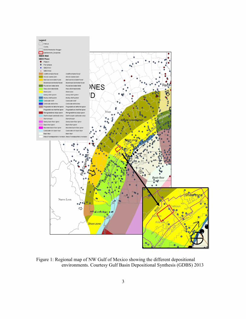
Figure 1: Regional map of NW Gulf of Mexico showing the different depositional
environments. Courtesy Gulf Basin Depositional Synthesis (GDBS)
2013.....................................................................................................3
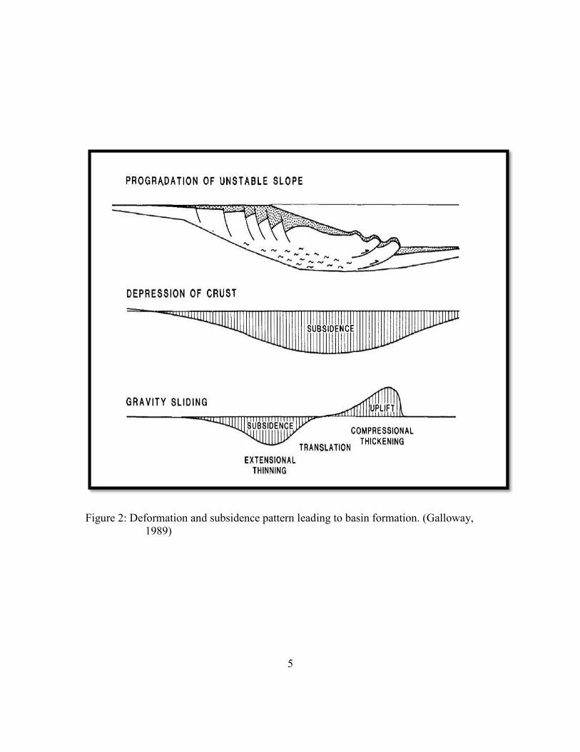
Figure 2: Deformation and subsidence pattern leading to basin formation. (Galloway,
1989) ...................................................................................................5
Figure 3: Sediment supply and dispersal axes for the northwestern and central parts of
Gulf of Mexico during the Cenozoic period. Red dashed rectangle shows
the approximate position of the study area. CZ = Carrizo; RG = Rio
Grande. (Modified from Galloway et al. 2000) ..................................6
Figure 4: Progressive Cenozoic shelf edge positions and sand-rich depocenters of
northwestern Gulf of Mexico. (Winker 1982 in Galloway 1989) .....7
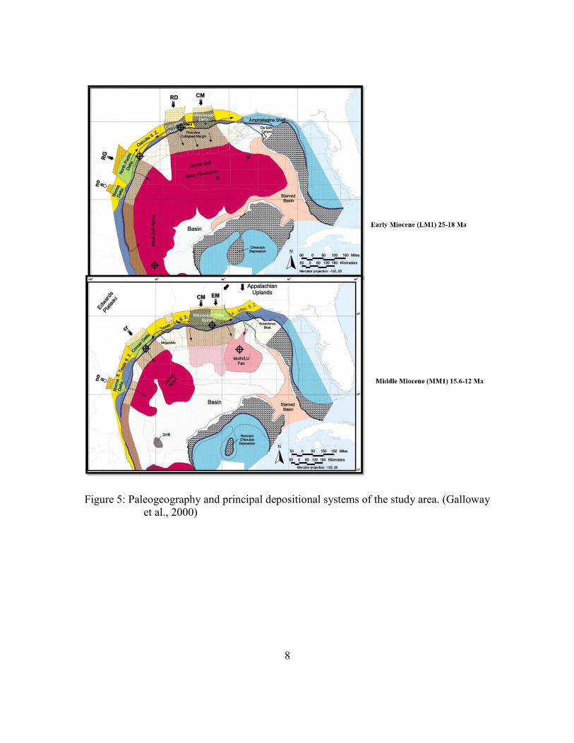
Figure 5: Paleogeography and principal depositional systems of the study area.
(Galloway et al., 2000)........................................................................8
Figure 6: Generalized dip-oriented stratigraphic cross section through the Rio Grande
depocenter, northwestern Gulf Coast sedimentary wedge. (Galloway,
1989). ..................................................................................................9
Figure 7: Map showing some principal structural features in Cenozoic GOM.
(Halbouty, 1966) ...............................................................................11
Figure 8: Area map of San Marcos map showing position of Refugio County (in red
rectangle). Approximate distance was calculated using the map.
(Halbouty, 1966) ...............................................................................12

x
Figure 9: Base map of Refugio County. See figure 1 for location map. Yellow circles
represent the positions of 17 Well logs in the study interval. The well
locations are represented this way in all maps. .................................14
Figure 10: An arbitrary seismic line showing horizons mapped and some well logs
with Spontaneous Potential (red), Gamma (black), Resistivity (blue)15
Figure 11. Miocene stratigraphy chart for the GOM basin. Complete chart shows the
entire stratigraphic sequences for the Cenozoic Period. Courtesy Gulf
Basin Depositional Synthesis (GBDS) 2013. ...................................16
Figure 12: The distribution of major coastal depositional environments. Prograding
(regressive) environments and retrograding (transgressive) environments
are highlighted. (Boyd et al., 1992) ..................................................19
Figure 13: Delta sub-environments: a) details of clinoforms formed in each sub-
environment, average distance covered by each section and extent of
dominant coastal processes. b) Map view of the typical components of a
delta (Goodbred and Saito 2012). .....................................................20
Figure 14: An example showing the morphology of a fluvial dominated delta system.
(Fisher et al 1969) .............................................................................21
Figure 15: Wave- influenced delta process formation. (Bhattacharya and Giosan
2003) .................................................................................................22
Figure 16: Typical shorezone and wave dominated delta vertical succession. A)
shorezone facies succession. B) Wave dominated delta facies
succession. (Modified from Clifton 2006, Bhattacharya and Walker
1991) .................................................................................................24
Figure 17: Typical shorezone profile. Red circles mark the principal environments
and their facies. (Walker and Plint, 1992) ........................................24

xi
Figure 18: Illustrative models showing the typical strandplain environments of
deposition. (Galloway and Cheng, 1985 in Ambrose. and Tyler, 1985)
...........................................................................................................25
Figure 19: Longitudinal profile of facies distribution in an incised valley. (Congxian
et al., 2006) .......................................................................................26
Figure 20: Facies sucession types within incised valley systems. (Congxian et al.,
2006) .................................................................................................27
Figure 21: Schematic illustration of (A) simple and (B) compound incised-valley
systems. Numbers 1-3 refer to successive episodes of cutting and filling
within the incised valley. PS= parasequence; FS = flooding surface.
(Zaitlin et al. 1994) ...........................................................................28
Figure 22: An illustration of a typical estuary environment. A) An estuary is
influenced by both marine and fluvial environments. B) The resultant
depositional environment with fluvial derived channels and marine
influenced sand bars. C) Estuaries contain heterogeneous deposits from
two sources. (Dalrymple et al. 1992 in Olariu 2014) ........................29
Figure 23: An example of gamma ray and spontaneous potential logs. Note the
difference in response between both logs in the sand-shale intervals and
also in the hydrocarbon saturated zone. (Fongngern 2011) ..............32
Figure 24: Typical well log response in fluvial and wave delta environments.
Deposits are overlain by MFS. (Bhattacharya and Walker 1991 in Olariu
2014) .................................................................................................33
Figure 25: Highstand delta well log pattern. (Bhattacharya and Walker 1991) ....34
Figure 26: Well log through a shoreface environment. (Modified from Bhattacharya
and Walker 1991) ..............................................................................35

xii
Figure 27: Typical dip section of incised valley fill and well log pattern. (Modified
from Allen and Posamentier, 1993 in Olariu 2014 and Fongngern 2011).
...........................................................................................................36
Figure 28: Well log pattern in an estuarine depositional environment. (Bhattacharya
1993) .................................................................................................37
Figure 29: seismic attribute comparison maps for H7, a) is a spectral decomposed
map generated using the variance volume .b) is spectral decomposed
map generated using the seismic volume. For corresponding variance
attribute map, see figure 38a. The channels are more visible in a. Both
maps are at a frequency of 25 Hz......................................................39
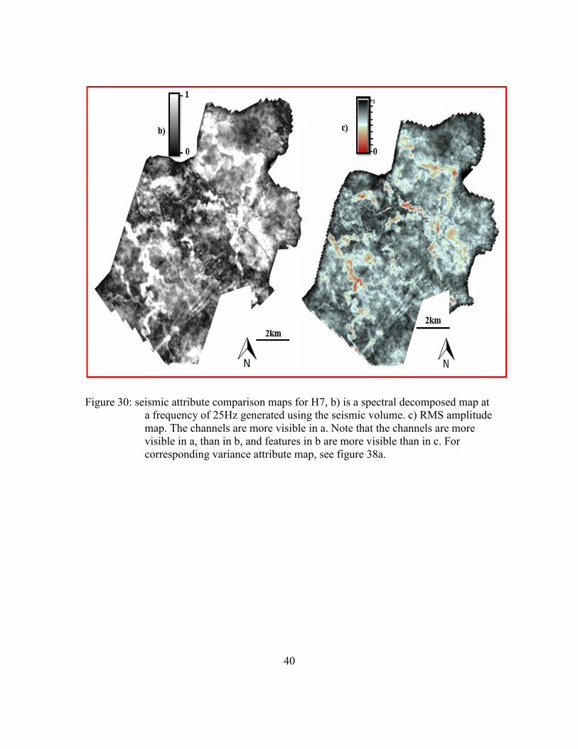
Figure 30: seismic attribute comparison maps for H7, b) is a spectral decomposed
map at a frequency of 25Hz generated using the seismic volume. c)
RMS amplitude map. The channels are more visible in a. Note that the
channels are more visible in a, than in b, and features in b are more
visible than in c. For corresponding variance attribute map, see figure
38a. ....................................................................................................40
Figure 31: Amplitude-variance map for H2; Anahuac shale interval. See figure 10 for
horizons positions .............................................................................41
Figure 32: Coarsening upward to blocky well log pattern observed between H2 and
H3. Purple arrows highlight the well log patterns. ...........................42
Figure 33: Amplitude-variance map of H5. Shoreline oriented deposits. Purple line
indicates thickness trend shown on the isochron map. .....................43
Figure 34: Isochron map between H3 and H5. Warm colors are low values, cool
colors are higher values. ...................................................................44
Figure 35: Net-sand isopach map between H3 and H5..........................................45

xiii
Figure 36: Variance attribute map for H4 showing first occurrence of fluvial deltaic
environment.. ....................................................................................47
Figure 37: Variance attribute map for H5. Presence of numerous channels indicate
further in-land position of the shoreline............................................48
Figure 38a: a) Amplitude variance map of H7 showing sinuous channels
characterized by minimal lateral migration, marked up areas in red are
shown in figure 38b ..........................................................................49
Figure 38b: b) Northeast-Southwest inclined feature of the short-lived strandplain. c)
distinctive channel present in the map northern axis for H7 ............50
Figure 38c: Figure c shows some features are more visible in the spectral decomposed
variance attribute maps. d) Figure d highlights the channel featured in c.
...........................................................................................................51
Figure 39a: Variance attribute map for H8 showing sinuous channels and valley cuts.
The red marked out portion is shown in figure 39b ..........................52
Figure 39b: Sinuous channels featured in H8 extending to the basin ....................53
Figure 40a: Variance attribute map for H9 featuring large channels. The red marked
out portion is shown in figure 40b. ...................................................54
Figure 40b: Numerous channels present within the H7 interval............................55
55
Figure 41a: Variance map for H11; larger valley scours appear in Younger intervals.
Red dashed rectangle highlights some incisional features. See figure
41b.....................................................................................................56
Figure 41b: Large west-east trending incisional features in H11 . ........................57
Figure 42: Variance map for H15 showing channels and valley cuts....................58

1
INTRODUCTION
OBJECTIVES
The Gulf of Mexico (GOM) basin has been intensively studied; however,
unexplained complexities remain. The objective of this project is a detailed depositional
analysis of the Miocene interval within Refugio County area to contribute to the
resolution of one of these GOM geological complexities. Refugio County is located along
the coastline of the Gulf of Mexico in the northeastern part of the Rio Grande basin
(Figure 1).
This research defines the depositional framework of the Miocene in Refugio
County with emphasis on identifying regressive and transgressive cycles to recognize
depositional episodes. Recognition of the depositional environment is based on
morphologic and evolutionary components, as classified by Boyd et al (1992). This
classification is founded on dominant coastal processes; it predicts responses in
geomorphology, facies and stratigraphy; identification of these responses help to group
them into regressive and transgressive categories - {sediment transport in response to sea
level changes, sediment influx and accommodation space}. With the use of a three
dimensional seismic data and well logs, I examined depositional patterns though time, the
structural and stratigraphic features present, the emergence, orientation and size of
channels and channel belts.
In addition, I examined the influence of the San Marcos Arch on deposition. The
Arch is a basement structural feature located towards the northeastern part of the study
area. Halbouty (1966) was of the opinion that the absence of salt controlled sediment
accumulations and thinning of sediment thickness towards the Arch prevails in the
Wilcox group, Frio and Miocene deposits; therefore the stratigraphic and structural

2
influence of the arch extends to the present GOM basin. The seismically imaged
stratigraphy of the Miocene Refugio County shows no influence associated with the
Arch. So, there may still be a structural signal that is best shown by thickness change in
the coastal deposits, but the Arch itself is not an influence in any of the geometries
associated with the depositional units.
3
Figure 1: Regional map of NW Gulf of Mexico showing the different depositional
environments. Courtesy Gulf Basin Depositional Synthesis (GDBS) 2013

4
BACKGROUND/PALEOGEOGRAPHY/DEPOSITIONAL HISTORY
Galloway (1987, 1989) suggested that the GOM basin was created by rifting,
followed by thermal subsidence of underlying transitional crust to oceanic crust. More
accommodation space was created by flexural loading from sediment deposition,
allowing for progradation of inner shelf facies and further seaward extension of the shelf
margin (Figure 2).
Miocene deposition in the GOM basin is characterized by basin stability;
sediment influx, dispersal rate, and shelfal out-building were modulated by eustatic
cycles. Sediment provenance (Figure 3) of the northwestern part of the GOM basin
during the Paleocene has been attributed to regional uplift and tectonism within the
continental interior of western North America (Galloway, 1989). During this time, the
geographic dispersion of depocenters around the northwest and central Gulf margins
reached their greatest extent. The Rio-Grande, Houston, and Mississippi embayment are
the major depocenters in the northwestern GOM basin. (Figure 4)
The North Padre and Norma deltas (Figure 5) were the prominent wave-
dominated shore-zone systems in the Rio Grande axis; narrow shelves surrounded these
deltas, which contained high volumes of sediment (Galloway et al., 2000). As these
deltas prograded, they created sand-rich wedges separated by updip tongues of marine
shale that were deposited during transgression and flooding of the shelf. These
successions of sandy wedges and marine shale reflect the idealized repetitive nature of
Cenozoic deposition (Figure 6). Successive episodes of progradation further builds the
shelf edge basinward and successive transgression does not reach as landward as its
antecedent (Galloway, 1989).
5
Figure 2: Deformation and subsidence pattern leading to basin formation. (Galloway,
1989)

6
Figure 3: Sediment supply and dispersal axes for the northwestern and central parts of
Gulf of Mexico during the Cenozoic period. Red dashed rectangle shows the
approximate position of the study area. CZ = Carrizo; RG = Rio Grande.
(Modified from Galloway et al. 2000)

7
Figure 4: Progressive Cenozoic shelf edge positions and sand-rich depocenters of
northwestern Gulf of Mexico. (Winker 1982 in Galloway 1989)
8
Figure 5: Paleogeography and principal depositional systems of the study area. (Galloway
et al., 2000)

9
Figure 6: Generalized dip-oriented stratigraphic cross section through the Rio Grande
depocenter, northwestern Gulf Coast sedimentary wedge. (Galloway, 1989).
After the Anahuac Shale transgression, the Lower Miocene depositional
succession includes fluvial systems, which served as direct supply of sediments to the
GOM basin. These systems contain reworked Cretaceous and older Cenozoic debris
sourced from uplift of the Edwards Plateau and adjacent inner coastal plain. This
depisode also contains barrier and strandplain systems; longshore currents reworked and
redistributed sand (both bed load and suspended sediments) along the shelf edge and
slope. These currents served as sediment transport media within the basin, albeit at a
slower rate than the fluvial systems. A short-lived transgressive episode at about 18 Ma
divides the Lower Miocene into two sequences, Lower Miocene 1 and 2 (LM1 and LM2).

10
During the Middle Miocene, high rate of deposition was recorded. The eastern
region was favored as sediment supply from western GOM to the northwest was pruned
by the Rio Grande Rift. The parched northern axis of the Rift was responsible for the low
volume of sediments transported from the highland to this axis. Nevertheless, sediments
from the revived Appalachian Mountains sourced deposition towards the northwestern
axis of the Gulf basin which compensated for its initial sediment deficiency at the
beginning of the Middle Miocene (Galloway et al. 2011). Sediment input was centered in
the Burgos basin in the northwestern GOM basin. The prominent delta system further
prograded the shelf margin about 25 mi (40 km). The wave- dominated Corsair delta,
advanced about 30 mi (50 km) depositing its thickest sands along the fault zone. This
sequence was also capped by a regional transgression of the shelf margin.
The Upper Miocene records more sediment accumulation in the central
Mississippi and east Mississippi portion of the GOM basin. Despite the sediment
dispersal shift from the northwestern part of the GOM basin, its margin was dominated
by a broad sandy strandplain. This was derived from reworked sediments from the
shrunken Coarsair, Rio Grande and Norma deltas and also from the Mississippi system.
STRUCTURAL HISTORY
The Cenozoic period of the northern GOM basin houses most of the complex
structural features (Galloway 2008). Strike–aligned growth-fault systems beneath the
coastal plain, clustered shallow salt stocks canopies beneath the slope region are some of
the structural features that are present within the GOM basin. These structures make good
stratigraphic and structural trap systems for hydrocarbons, creation of minibasins and
also, influence deposit thickness variability.

11
The San Marcos Arch is an extension of the Llano Uplift; it separates the Houston
and Rio Grande basins (Figure 7); and is on the northeastern axis to the Refugio County
(Figure 8). Sediment accumulation thins with proximity to and over the arch, this effect is
significant from the Jurassic to the Miocene periods (Halbouty, 1966). The Arch is house
to several oil and gas exploration and exploitation activities owing to its wealth of
stratigraphic and structural traps.
Figure 7: Map showing some principal structural features in Cenozoic GOM. (Halbouty,
1966)

12
Figure 8: Area map of San Marcos map showing position of Refugio County (in red
rectangle). Approximate distance was calculated using the map. (Halbouty,
1966)

13
METHOD OF INVESTIGATION
The data set used is a three-dimensional (3D) seismic volume of about 106 square
miles (275 square kilometers), with bin size 25 m by 25 m, dominant frequency range of
30 to 45 Hz, and typical vertical resolution of about 53 to 70 ft. (16 to 21 m). I used the
Landmark software to define and analyze structural and stratigraphic architecture within
the dataset. Data quality was adequate. The area of interest covered a depth of 1050 ft. to
about 5000 ft. (about 400 to 1500 milliseconds): the top of the Anahuac Shale to the top
of the Miocene interval. 17 wireline logs were integrated within the seismic data (Figure
9); 15 of them had a length exceeding the depth of interest (Figure 10). I used gamma
ray, spontaneous potential, and resistivity curves as guides in mapping some horizons
(Figure 10); notably the base and top of the Anahuac Shale. Well control data from this
area was provided by the Gulf Basin Depositional Synthesis (GBDS) research group; this
age data indicates that the entire studied section positioned above the Anahuac Shale is
Early Miocene. Regional correlations confirm that all deposits studied above Anahuac are
bounded above by the Middle Miocene horizon, making the entire section Early Miocene
in age. The well log correlation to the Anahuac Shale was aided by the stratigraphic
section benchmark chart also courtesy the (GBDS) research group (Figure 11). The
remaining 15 horizons were picked at strong amplitude events separated vertically by 30-
100 milliseconds. All of the picked horizons were interpolated and filtered.

14
Figure 9: Base map of Refugio County. See figure 1 for location map. Yellow circles
represent the positions of 17 Well logs in the study interval. The well
locations are represented this way in all maps.

15
Figure 10: An arbitrary seismic line showing horizons mapped and some well logs with
Spontaneous Potential (red), Gamma (black), Resistivity (blue)

16
Figure 11. Miocene stratigraphy chart for the GOM basin. Complete chart shows the
entire stratigraphic sequences for the Cenozoic Period. Courtesy Gulf Basin
Depositional Synthesis (GBDS) 2013.
The mapped horizons were converted to various seismic attributes to identify the
one that would yield the best visualization of relevant features within the data. Some of
the attributes experimented with in this study include variance, root mean squared
amplitude (RMS), and spectral decomposition. The variance attribute is similar to the
semblance but gives better resolution than semblance. It is used to detect lateral seismic
changes that often relate to geologic changes such as faults, facies changes and other
geologic patterns. The attribute volume was generated in Petrel and loaded into the

17
Seiswork application in Landmark. RMS extraction detects major stratigraphic and
lithologic changes, typically sand/shale ratio. Seismic attribute extraction maps were
created between horizons and and along horizons using a 16 millisecond window.
The spectral decomposition tool generates several volumes from a single volume
input and each of these volumes represents a different frequency band (D.
Subrahmanyam and P.H. Rao, 2008). Smaller structures are more visible at higher
frequencies and larger structures are visible at lower frequencies. The seismic volume
and variance attribute volume were individually used as input volumes. Spectra1
decomposed maps and spectra1 decomposed variance maps were generated along each
horizon using a 16 millisecond window, for a frequency range of 0 – 125 Hz.
In order to determine the effect of the San Marcos Arch to sedimentation, I made
use of the gamma ray logs to make quantitative sand estimates. The method entails the
following steps: (1) Determine gamma ray sand cut-off value in each well. (2) Using the
cut-off value, sand-rich interval thicknesses are added together to give net sand thickness
within the interval of interest. The interval of interest referred to in this case is an interval
bounded by two horizons. Eight horizons were used as reference intervals, and sand
intervals defined by the cut-off gamma ray value, were counted in each well between two
horizons. Total sand thickness for each interval was individually annotated against its
reference well; this was used to produce contoured net sand maps.

18
CLASTIC DEPOSITIONAL SYSTEMS
The shelf region of the continental margin consists of different depositional
environments; and are classified as coastal and shallow marine (Figure 12); few of them,
with relevance to this study will be discussed. The creation of these environments is
based on certain factors; such as sea level changes, regression and transgression,
sediment caliber and influx, evolutionary and morphological changes based on dominant
coastal processes (Boyd et al., 1992).
DELTAS
The deltaic environment represents sediments discharged by a river into a
standing body of water. With more sediment influx, progradation occurs across the shelf,
some of these deposits form subaerially and some are formed subaqueously. There are
four geomorphic environments of deposition; predelta, delta plain, delta front and
prodelta (Figure 13); the prodelta is the most proximal to the receiving basin
(Bhattacharya, 2006). Deltas are subdivided into three; fluvial, wave and tide dominated
deltas. This classification represents the dominant marine processes that occur at the river
mouth bar.
DELTA CLASSIFICATION
Fluvial dominated deltas
Fluvial dominated deltas are not morphologically influenced by waves and tides.
Therefore multiple coeval distributary channels form, some with wide orientation.
Channel pattern is sinuous to anastomose. A lobate or elongate shaped delta is usually

19
formed (Figure 14) and this concentrates sediments into a smaller surface area; sediments
deposition into the basin is faster when compared to a wave dominated delta.
Figure 12: The distribution of major coastal depositional environments. Prograding
(regressive) environments and retrograding (transgressive) environments are
highlighted. (Boyd et al., 1992)

20
Figure 13: Delta sub-environments: a) details of clinoforms formed in each sub-
environment, average distance covered by each section and extent of
dominant coastal processes. b) Map view of the typical components of a
delta (Goodbred and Saito 2012).

21
Figure 14: An example showing the morphology of a fluvial dominated delta system.
(Fisher et al 1969)
Wave dominated deltas
Waves deflect sediment from the river mouth, with the influence of longshore
wave energy. Deposition occurs on both sides of the distributary channels generally
referred to as sand spits (Bhattacharya and Giosan, 2003). This generally results in
massive sand accumulation in a shoreline parallel position (Figure 15), and this leads to
the development of sandy beaches by longshore bars.
Tide dominated deltas
The tide dominated delta environment contains tidally reworked deposits.
Channels have few distributary channels that are usually short lived. This environment
forms during a highstand period of the sea level and thus usually subaqueous. The

22
heterolithic nature of sedimentary successions generally present in tide dominated deltaic
settings, is formed as a result of the typical inconsistency of tidal energy level (Goodbred
and Saito 2012). In tide dominated deltas, mud deposits are predominant in the prodelta
and also occur as overbank deposits (Bhattacharya, 2006).
Figure 15: Wave- influenced delta process formation. (Bhattacharya and Giosan 2003)

23
SHOREZONE
The shorezone depositional section is created by wave processes and has similar
lithological facies to a wave dominated delta (Figure 16). Slower rate of sediment influx
may inhibit progradation rate; sediment reworking by waves thrives in this condition and
this leads to extensive shorezone formation. The foreshore, shoreface and off-shore
(Figure 17), are the three wave energy defining limits that make up the shorezone
environment (Walker and Plint, 1992). In terms of grain size and facies, the shoreface is a
transitional marker between the two end-member environments; typically, a change from
sand to mud on the seaward extent of the shorezone.
STRANDPLAINS
Strandplains represent the regressive marine reworked depositional features
usually located in a coastal plain environment. They are generally created by
redistribution of river mouth sediments by longshore currents. Strandplains are classified
based on the degree of sediment heterogeneity and facies architecture (Figure 18); they
are grouped into beach-ridge plains and Chenier plains (Ambrose and Tyler, 1985).
The beach-ridge complex is a strike- elongate mass of prograded beach ridges,
containing three sub-complexes; a sandy beach-ridge complex, a sandy shoreface and a
transecting fluvial-deltaic complex. The beach-ridges contain massive and mostly
homogenous thick beach and dune sands. Fluviodeltaic channels cutting through the
beach consists of upward-fining channel sandstones.
Chenier plains consist are part of the sandy strandplain system. They are
generated from wave reworked sand deposits and are characterized by mud flat intrusions
(Owen D.E. 2008). Well log signature is usually characterized by an upward-fining trend.
Other sub-complexes include; Chenier strike elongated sand bodies and fluvioestuarine
complexes.

24
Figure 16: Typical shorezone and wave dominated delta vertical succession. A)
shorezone facies succession. B) Wave dominated delta facies succession.
(Modified from Clifton 2006, Bhattacharya and Walker 1991)
Figure 17: Typical shorezone profile. Red circles mark the principal environments and
their facies. (Walker and Plint, 1992)

25
Figure 18: Illustrative models showing the typical strandplain environments of
deposition. (Galloway and Cheng, 1985 in Ambrose. and Tyler, 1985)
INCISED VALLEYS
During relative sea level fall, the scouring ability of fluvial systems creates down
cutting valleys. Rapid fall below the shelf margin commonly creates canyons; these
valleys are assumed to be possible medium of sediment transport to the basin (Vail et al.
1984). Incised valleys can be differentiated from channels in terms of size and geometry;
channels are usually smaller than and not as wide as incised valleys (Gibling, 2006).

26
Sediment fill of the valleys usually occur during sediment retrogradation and also through
fluvial deposits prograding even during a sea level rise (Zaitlin et al., 1994). The facies
differ between the fluvial influenced deposits and the marine flooding deposits,
classically with coarser sand at the base overlain with sediments in an upwarding fining
trend in the river filled valleys and the marine filled valleys containing structure-less
muddy sediments and poorly sorted sands (Figure 19). Nevertheless, an incised valley fill
may represent sediments derived from both marine and river environments (Figure 20)
An incised valley system can be subjected to multiple episodes of cuts and fills
(Figure 21), this creates a complex or compound incised valley system (Zaitlin et al.,
1994). Within these systems, parasequence sets exist; this usually creates challenges in
chronostratigraphic grouping of sediments. The age defining boundaries such as
maximum flooding surfaces and sequence boundaries are usually obscured.
Figure 19: Longitudinal profile of facies distribution in an incised valley. (Congxian et
al., 2006)

27
Figure 20: Facies sucession types within incised valley systems. (Congxian et al., 2006)

28
Figure 21: Schematic illustration of (A) simple and (B) compound incised-valley
systems. Numbers 1-3 refer to successive episodes of cutting and filling
within the incised valley. PS= parasequence; FS = flooding surface. (Zaitlin
et al. 1994)
ESTUARY
During transgression, sediments back-stepping will sink into valleys created
during the sea falling stage. The submerged valley deposit is referred to as an estuary;
depending on the prevailing marine conditions, an estuary will be tide dominated or wave
dominated. Estuaries represent a transition zone between marine and fluvial
environments (Figure 22) and thus, receive sediments from both sources (Dalrymple,
2006)

29
Figure 22: An illustration of a typical estuary environment. A) An estuary is influenced
by both marine and fluvial environments. B) The resultant depositional
environment with fluvial derived channels and marine influenced sand bars.
C) Estuaries contain heterogeneous deposits from two sources. (Dalrymple
et al. 1992 in Olariu 2014)

30
WELL-LOG REFLCTIONS IN DEPOSITIONAL ENVIRONMENTS
Well logs provide useful information that aid sedimentary basins investigations. The
lithology logs- gamma ray, spontaneous potential were employed in this study. In a shale
dominated zone, the spontaneous potential log deflects towards zero; shale is a low
porosity and relatively impermeable rock type.
The gamma ray lies along the left-hand side of the log (Figure 23), it measures natural
gamma radiation in the rock and records high values at such intervals. The spontaneous
potential also lies along the left-hand side of the log; it estimates the permeability of the
rock. I observed that some areas showing presence of sand on the gamma log pattern
appeared nil on the spontaneous potential logs, the electro chemical contrast between the
bore-hole and rock fluids may not be significant (Galloway and Hobday 1983). For
example, deeper formations typically have more saline waters than well log fluids; this
disparity yields a leftward curve log response within porous and permeable intervals.
Sand intercalated with mud could have low porosity and permeability, thus gamma ray
logs were used mostly and spontaneous potential logs were used in their absence.
Spontaneous potential logs are also sensitive to the presence of hydrocarbon (Figure 23),
and it will record reading in intervals where the pore space is filled with hydrocarbon
(Torres-Verdin 2010).
Wireline log signatures have been successfully used to define depositional cycles in the
Cenozoic GOM (Van Wagoner et al. 1990, Robert G. Loucks et al. 2011, Brown et al.
2005, Fongngern and Ambrose 2012). Though they used the gathered information from
the well logs in combination with other data to build sequence stratigraphic models for

31
their specific studied sections, certain general depositional styles for strata of the
Cenozoic GOM have been established.
Deltas
Deltas typically showcase an upward coarsening well-log pattern (Bhattacharya
and Walker 1991). They are bounded on top by a significant transgressive surface
referred to as maximum flooding surface (MFS); MFS is a stratigraphic surface that
represents the end of retrogradation of marine sediments (Figure 24). Following this
surface is typically progradation of highstand (high sea level) deltaic sediments (Figure
25). Wave dominated deltas show a blockier pattern, this indicates less mud present.
Shorezone
Shoreface and strandplain/beach environments typically consist of massive sand
deposits, and hence portray a blocky, but overall upward coarsening pattern. These
characteristics are similar to a wave dominated delta; they can be differentiated by the
sharp basal contact with the underlying mud deposits observed in shoreface deposits
(Figure 26).
Incised valleys
Incised valley fills record multiple facies usually with a basinward shift in facies
at the base (Figure 27). Well log records a sharp base and blocky aggradational sand
body, overlain by an upward fining trending sedimentation. Typically, estuaries are part
of incised valleys fills.

32
Estuaries
Estuaries generally exhibit an upward fining well log trend (Figure 28). The basal
component is usually marine derived sand bodies, which has been interpreted as bay-head
deltaic sediments. This delta is smallest of deltas, during sea level rise, the delta is moved
back into an incised valley; forming the early part of transgressive deposits (Dalrymple et
al 1992).
Figure 23: An example of gamma ray and spontaneous potential logs. Note the difference
in response between both logs in the sand-shale intervals and also in the
hydrocarbon saturated zone. (Fongngern 2011)

33
Figure 24: Typical well log response in fluvial and wave delta environments. Deposits are
overlain by MFS. (Bhattacharya and Walker 1991 in Olariu 2014)

34
Figure 25: Highstand delta well log pattern. (Bhattacharya and Walker 1991)

35
Figure 26: Well log through a shoreface environment. (Modified from Bhattacharya and
Walker 1991)

36
Figure 27: Typical dip section of incised valley fill and well log pattern. (Modified from
Allen and Posamentier, 1993 in Olariu 2014 and Fongngern 2011).

37
Figure 28: Well log pattern in an estuarine depositional environment. (Bhattacharya
1993)
38
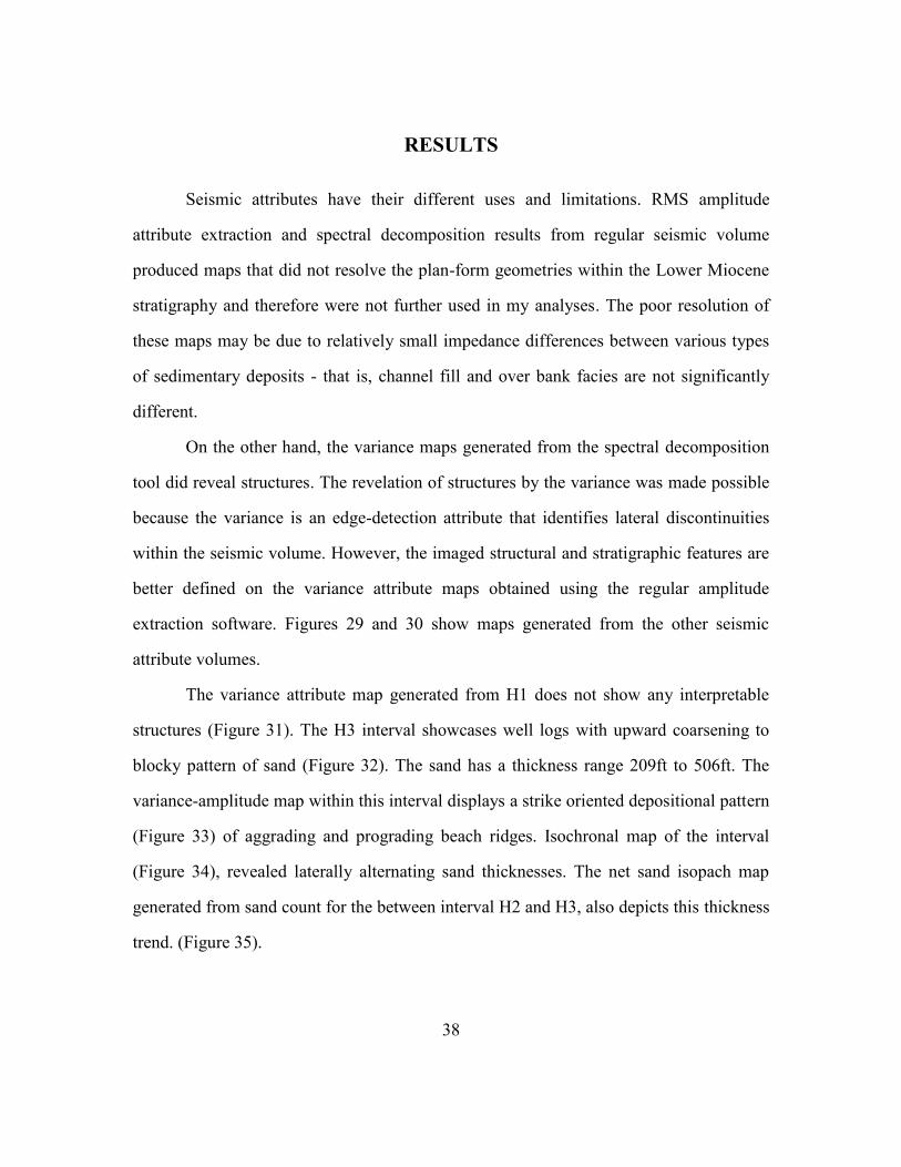
RESULTS
Seismic attributes have their different uses and limitations. RMS amplitude
attribute extraction and spectral decomposition results from regular seismic volume
produced maps that did not resolve the plan-form geometries within the Lower Miocene
stratigraphy and therefore were not further used in my analyses. The poor resolution of
these maps may be due to relatively small impedance differences between various types
of sedimentary deposits - that is, channel fill and over bank facies are not significantly
different.
On the other hand, the variance maps generated from the spectral decomposition
tool did reveal structures. The revelation of structures by the variance was made possible
because the variance is an edge-detection attribute that identifies lateral discontinuities
within the seismic volume. However, the imaged structural and stratigraphic features are
better defined on the variance attribute maps obtained using the regular amplitude
extraction software. Figures 29 and 30 show maps generated from the other seismic
attribute volumes.
The variance attribute map generated from H1 does not show any interpretable
structures (Figure 31). The H3 interval showcases well logs with upward coarsening to
blocky pattern of sand (Figure 32). The sand has a thickness range 209ft to 506ft. The
variance-amplitude map within this interval displays a strike oriented depositional pattern
(Figure 33) of aggrading and prograding beach ridges. Isochronal map of the interval
(Figure 34), revealed laterally alternating sand thicknesses. The net sand isopach map
generated from sand count for the between interval H2 and H3, also depicts this thickness
trend. (Figure 35).

39
Figure 29: seismic attribute comparison maps for H7, a) is a spectral decomposed map
generated using the variance volume .b) is spectral decomposed map
generated using the seismic volume. For corresponding variance attribute
map, see figure 38a. The channels are more visible in a. Both maps are at a
frequency of 25 Hz.
40
Figure 30: seismic attribute comparison maps for H7, b) is a spectral decomposed map at
a frequency of 25Hz generated using the seismic volume. c) RMS amplitude
map. The channels are more visible in a. Note that the channels are more
visible in a, than in b, and features in b are more visible than in c. For
corresponding variance attribute map, see figure 38a.

41
Figure 31: Amplitude-variance map for H2; Anahuac shale interval. See figure 10 for
horizons positions

42
Figure 32: Coarsening upward to blocky well log pattern observed between H2 and H3.
Purple arrows highlight the well log patterns.

43
Figure 33: Amplitude-variance map of H5. Shoreline oriented deposits. Purple line
indicates thickness trend shown on the isochron map.

44
Figure 34: Isochron map between H3 and H5. Warm colors are low values, cool colors
are higher values.

45
Figure 35: Net-sand isopach map between H3 and H5.

46
The overlying intervals from the top of H3-H6, shows a coastal plain environment
consisting of deposits filling channels and channel belts with no obvious structures
defining erosional valley walls (Figures 36&37). Maximum channel-belt length
Maximum channel-belt length is approximately 21000ft and widths range between 330-
3000ft. Well log pattern is mostly serrated, with intermittent occurrence of thick shale or
sand bodies.
Abundance of channels and channel belts dominate the interval above at depth
3000ft (H7). Channels are sinuous but exhibit little lateral migration (i.e., no laterally
continuous point-bar deposits). The first incised valleys observed in Lower Miocene
strata are shown in Figures 38&39. Measured valley length ranges from 6360-35200ft,
and widths for the erosional structures vary between 445-2300ft. Notice that these valleys
also preserve remnant topographic highs within them (Figure 38). Towards the
southwestern axis of this map, an under developed beach structure is exhibited. Well log
at this interval exhibits an upward coarsening pattern with an extensive basal shale
response.
Moving up through the volume into younger strata- H9 to H11, the dominant
stratigraphic features are channels and incised valleys. The valley walls are characterized
by larger scoops with more curvature that match the form of the outer banks of migrating
river bends (Figures 40 &41). Well logs transecting some of these features showed
presence of sands. Valley dimensions range from 2,590-3,650ft wide and 9,853 -15,000ft
Long. The variance attribute maps for the youngest intervals H12 to H15 do not clearly
show structures when compared to older sections (Figure 42).

47
Figure 36: Variance attribute map for H4 showing first occurrence of fluvial deltaic
environment..

48
Figure 37: Variance attribute map for H5. Presence of numerous channels indicate further
in-land position of the shoreline.

49
Figure 38a: a) Amplitude variance map of H7 showing sinuous channels characterized by
minimal lateral migration, marked up areas in red are shown in figure 38b

50
Figure 38b: b) Northeast-Southwest inclined feature of the short-lived strandplain. c)
distinctive channel present in the map northern axis for H7

51
Figure 38c: Figure c shows some features are more visible in the spectral decomposed
variance attribute maps. d) Figure d highlights the channel featured in c.

52
Figure 39a: Variance attribute map for H8 showing sinuous channels and valley cuts. The
red marked out portion is shown in figure 39b

53
Figure 39b: Sinuous channels featured in H8 extending to the basin

54
Figure 40a: Variance attribute map for H9 featuring large channels. The red marked out
portion is shown in figure 40b.

55
Figure 40b: Numerous channels present within the H7 interval

56
Figure 41a: Variance map for H11; larger valley scours appear in Younger intervals. Red
dashed rectangle highlights some incisional features. See figure 41b.

57
Figure 41b: Large west-east trending incisional features in H11 .

58
Figure 42: Variance map for H15 showing channels and valley cuts

59
DISCUSSION AND CONCLUSIONS
Analysis of the morphological pattern of seismically imaged stratigraphic features
and associated deposits provides information about its depositional processes. The study
interval includes the Oakville Sandstone that marks the basal Miocene and the overlying
Fleming formation. The seismically imaged stratigraphic maps show that after the
Anahuac Shale Formation, the coastline was built of prograding beach ridges
characteristic of a wave dominated coast and considerable alongshore transport and
accumulation of sand. The beach ridges have the greatest volume of sand within the
section, and this is a common occurrence of any early Miocene coastal depositional
system. Galloway et al. (2000), Galloway, (1987, 1999) reported that sediment
provenance during the Lower Miocene was from the North Padre and Norma deltaic
complexes on the northeast and the Calcasieu and Mississippi deltas on the southwestern
axes of the GOM. (See figure 5).
The fluvially dominated coastal section was first dominated by channel belts and
later by incised valleys and channel belts. Channels remained characteristically sinuous
and single-thread through the section. Evidence of rapid transgressions and regression in
map view are rare. The only example is shown in Figure 38; rapid transgressions and
regressions do not produces regionally preserved stratigraphy because much of the strata
appear to be cut out by later channel belts and valleys.
The change from strandplain to fluvial environment is characterized by changes
in sedimentary structures, appearance of channels and incised valley cuts. Sinuous,
single-thread fluvial channel deposits appear to dominate the stratigraphy of the non-
marine environments characterizing the overall coastal progradation recorded by the
Lower Miocene strata. The dip orientated channels extend to the edge of the study area

60
and do not show signs of thinning out (Figure 43). It is evident that, they served as
sediment supply to the prograding coast and at the largest scale to the Cenozoic shelf-
margin out-build. The subtle change in style of valley walls as we move up the section,
suggest the change in channel character. In addition, increase in width of the valleys
indicates further in-land position of the younger strata.
The alternating wireline signatures from upward coarsening to upward fining,
reveals the repetitive Cenozoic depositional pattern described by previous studies in other
parts of the Gulf basin (Galloway 1989, Loucks et al. 2011, Fongngern and Ambrose,
2012). Fluvial to delta to delta-fed apron and coastal plain to shore-zone to shelf to shelf-
fed apron, are the depositional systems groups that were observed within the study as
categorized by (Galloway et al. 2000) for the Cenozoic genetic sequences of the Gulf
basin.
Interpretation of this data leaned more on the amplitude variance maps generated.
Well logs were widely spaced and few and these hindered regional strata correlations.
The map patterns largely show a regressive depositional history dominated by a
shorezone system and younger channels, channel belts and incised valleys. The observed
stratigraphy and structures also reveal that the San Marcos Arch was not active during the
Lower Miocene.
The stratigraphic evidence includes
(1) Straight beach ridges that suggest the arch is not adding local curvature to the
coastline.
(2) Channel belts that show no evidence of deflection in orientation by a potential
topographic high.
(3) Incised valleys that display no spatial change in scale that might be expected
by relative arch uplift to the northeast.

61
The structural evidence for no arch activity during the Lower Miocene is no large
scale change in sediment thickness from southwest to northeast that would be expected
by a subsidence pattern associated with active arch tectonism.

62
REFERENCES
Ambrose, A.W. and Tyler N., 1985, Facies architecture and production
characteristics of strandplain reservoirs in the Frio Formation, Texas. Bureau of
Economic Geology. Report of Investigations No. 146.
Bhattacharya, J.P. and Walker, R.G., 1991, Facies and facies sucessions in river
and wave dominated depositional systems of the Upper Cretaceous Dunvegan Formation,
northwestern Alberta. Bulletin of Canadian Petroleum Geology, v. 39, no.2 p. 165-191.
Bhattacharya, J.P., 1993, The expression and interpretation of marine flooding
surfaces and erosional surfaces in core; examples from the Upper Cretaceous Dunvegan
Formation, Alberta foreland basin, Canada. Special Publication International Association
sedimentologist, v. 18,p. 125-160
Bhattacharya,,J.P.and Giosan, L., 2003,Wave–influenced deltas:
geomorphological implications for facies reconstruction. Sedimentology v. 50, p. 187-
210.
Bhattacharya, J. P, 2006, Deltas. Facies Models revisited, Society for Sedimentary
Geology (SEPM) Special Publication No.4, p. 237-292.
Boyd, R., Dalrymple R., and Zaitlin, B.A., 1992, Classification of clastic coastal
depositional environments. In: Donoghue J.F, Davis R.A, Fletcher C.H. and Suter J.R.
(Editors), Quaternary Coastal Evolution. Sedimentary Geology, v. 80, p. 139-150.
Dalrymple, R.W., Zaitlin, B.A., and Boyd, R., 1992, Estuarine facies models:
conceptual basis and stratigraphic implications. SEPM, Journal of sedimentary petrology,
v. 62, no. 6, p. 1130-1146.
Owen, D.E., 2008, Geology of the Chenier Plain of Cameron Parish,
southwestern Louisiana. ed.: Geological Society of America Field Guide 14, 2008 Joint
Annual Meeting, Houston, Texas, p. 27–38
Clifton, H.E., 2006, A reexamination of facies models for clastic shorelines. In:
Posamentier, HW, and Walker, RG, eds, Facies Models Revisited: SEPM, Special
Publication, v. 84, p. 293–337.
Congxian, Li, Ping Wang, Daidu Fan and Shouye Yang, 2006, Characteristics and
Formation of Late Quaternary incised-valley-fill sequences in sediment-rich deltas and
estuaries: Case studies from C hina SEPM Special Publication No. 85, p. 30

63
Fisher, W.L., Brown, L.F., Scott, A.J. and McGowen, J.H., 1969. Delta Systems
in the Exploration for Oil and Gas. Bur. Econ. Geol., University of Texas, Austin, p. 78.
Galloway, W. E., and Hobday, D. K., 1983, Terrigenous clastic depositional
systems. Applications to petroleum, coal and uranium exploration: Springer-Verlag,New
York, NY, pp. 7, 420.
Galloway, W. E., and Cheng, E.S., 1985, Reservoir facies architecture in a
microtidal barrier system— Frio Formation, Texas Gulf Coast: The University of Texas
at Austin, Bureau of Economic Geology Report of Investigations No. 144, p36 In:
William E. Galloway 1987, Depositional and structural architecture of prograding clastic
continental margins: tectonic influence on patterns of basin filling. Norsk Geologisk
Tidsskrift, Vol. 67, pp. 237-251. Oslo 1987. ISSN 0029-196X.
Galloway, W. E., 1989, Genetic stratigraphic sequences in basin analysis II:
Application to Northwest Gulf of Mexico Cenozoic basin. AAPG Bulletin, v. 73, no. 2p.
143-154.
Galloway, W. E., Ganey-Curry, P., Xiang Li, and Richard, T. B., 2000, Cenezoic
depositional history of the Gulf of Mexico basin. AAPG Bulletin, v. 84, no. 11 p. 1743-
1774.
Galloway, W. E., 2008, Depositional Evolution of the Gulf of Mexico
Sedimentary Basin. Sedimentary Basins of the World, v. 5 p. 505- 549.
Galloway, W. E., Whiteaker, T. L. and Ganey-Curry, P., 2011, History of
Cenozoic North American drainage basin evolution, sediment yield, and accumulation in
the Gulf of Mexico basin. Geological Society of America Geosphere, v.7 no. 4 p. 938-
973.
Gibling, R. M., 2006, Width and thickness of fluvial channel bodies and valley
fills in the geological record: A literature compilation and classification. SEPM, v. 76,
p.731-770.
Goodbred, S.L. and Saito, Y., 2012, Tide dominated deltas. In: R.A Davis Jr. and
R.W. Dalrymple (eds), Principles of Tidal Sedimentology: Springer science and Business
media.
Halbouty M. T., 1966, Stratigraphic-Trap Possibilities in Upper Jurassic Rocks,
San Marcos Arch, Texas. American Association of Petroleum Geologist. v. 50 pp. 3-24.
Olariu C., 2014, Estuaries and Incised valleys. Clastic Depositional Systems.
Personal Communication.

64
Posamentier, H.W. and Allen, G.P., 1993, Variability of the sequence
stratigraphic model: effects of local basin factors: Sedimentary Geology, v. 86, p. 91–
109. In Cornel Olariu, C., 2014, Clastic Depositional Systems. Personal communication.
Rattanaporn, F., 2011, Sequence Stratigraphy, Sandstone Architecture, and
Depositional Systems of the Lower Miocene Succession in the Carancahua Bay Area,
Texas Gulf Coast. Master’s Thesis, The University of Texas at Austin. p.56
Rattanaporn, F. and Ambrose, W. A., 2012, Variability of Sandstone Architecture
and Bypass Systems of the Miocene Oakville and Lower Lagarto Formations in the
Carancahua Bay Area, Texas Gulf Coast. Gulf Coast Association of Geological Societies
Transactions, v. 62, p. 131–144.
Robert, G. L., Brian, T. M., and Hongliu. Z., 2011, On-shelf lower Miocene
Oakville sediment-dispersal patterns within a three-dimensional sequence-stratigraphic
architectural framework and implications for deep-water reservoirs in the central coastal
area of Texas. AAPG Bulletin, v. 95, no. 10, p. 1795–1817.
Subrahmanyam, D. and Rao, P.H., 2008, Seismic attributes –A review. 7th
International Conference & Exposition on Petroleum Geophysics.
Vail, P. R., Hardenbold, J., and Todd, R. G., 1984. Jurassic unconformities,
chronostratigraphy, and sea-level changes from seismic stratigraphy and biostratigraphy.
In: Schlee J. S. (Ed), Interregional unconformities and Hydrocarbon Accumulation.
American Association of petroleum Geology, Memoir v. 36 p. 129-144.
Van Wagoner, J.C., Posamentier, H. W., Mitchum, R. M., Vail, P.R., Sarg, J.F.,
Loutit, T.S. and Hardenbol, J., 1988, An overview of sequence stratigraphy and key
definitions. In: C.W. Wilgus et al., eds., Sea level changes: an intergrated approach.
Society of Economic Paleontologists and Mineralogists Special Publication v.42 p. 39-
45.
Van Wagoner, J. C., Mitchum, R. M, Campion, K. M., and Rahmanian, V. D.,
1990, Siliciclastic sequence stratigraphy in well logs, cores, and outcrops: AAPG
Methods in Exploration series 7, p.55.
Walker, R. G. and Plint, A. G., 1992, Wave and Storm dominated shallow marine
systems, in: Walker, R. G. and James, N. P. (eds), Facies Models, response to sea level
change. Geological Association of Canada, p. 219-238.
Winker C.D., 1982, Cenozoic shelf margins, northwestern Gulf of Mexico basin:
Gulf Coast Association of Geological Societies Transactions, v. 32, p. 427-448. In:
William E. Galloway, 1989, Genetic stratigraphic sequences in basin analysis II:

65
Application to Northwest Gulf of Mexico Cenozoic basin. AAPG Bulletin, v. 73, no. 2p.
143-154.
Zaitlin, B.A., Dalrymple, R.W., and Boyd, R., 1994, The stratigraphic
organization of incised-valley systems associated with relative sealevel change, in
Dalrymple, R.W., Boyd, R., and Zaitlin, B.A., eds., Incised-Valley Systems: Origin and
Sedimentary Sequences: SEPM, Special Publication 51, p. 45–62.
Gulf of Mexico Basin Cenozoic Chronostrostragraphic Designations and
Biostratigraphic Datums Chart, 2013. Version 18, Gulf of Mexico Basin Depositional
Synthesis (GDBS). The University of Texas at Austin