copyright 2020, john sena akoto
TRANSCRIPT

Deep Seismic Structure of Aleutian Subduction Zone Using Teleseismic PdP and SdS Precursor Functions
by
John Sena Akoto, B.S.
A Thesis
In
Geoscience
Submitted to the Graduate Faculty of Texas Tech University in
Partial Fulfilment of the Requirements for
the Degree of
MASTER OF SCIENCE
Approved
Dr. Harold Gurrola Chair of Committee
Dr. George Asquith
Dr. Dustin Sweet
Mark Sheridan Dean of the Graduate School
December, 2020

Copyright 2020, John Sena Akoto

Texas Tech University, John Sena Akoto, December 2020
ii
ACKNOWLEDGMENTS
First and foremost, I would like to thank Dr. Harold Gurrola. With his support and guidance, I
was able to successfully complete this thesis. He provided much help with Matlab
programming and with understanding complex geophysical concepts. He pushed me to work
more independently and trust my ability.
Next, I extend my gratitude to Dr. George Asquith and Dr. Dustin Sweet. They offered their
time and assisted in several ways. I would also like to thank Tiffany Wiley and Abdul Hafiz
Issah; their collaboration on aspects of my thesis helped to make it a success. I greatly
acknowledge Hannah Snidman for proofreading this thesis and checking for grammar.
Finally, I could not have completed this thesis without financial support from the Texas Tech
University Geoscience Department.

Texas Tech University, John Sena Akoto, December 2020
iii
TABLE OF CONTENTS
ACKNOWLEDGMENTS ............................................................................................................ ii
ABSTRACT ............................................................................................................................... v
LIST OF FIGURES ................................................................................................................... vi
1 INTRODUCTION................................................................................................................ 1
1.1 Background ................................................................................................................ 1
1.2 Purpose and Objectives of the Study ......................................................................... 2
2 LITERATURE REVIEW ..................................................................................................... 3
2.1 Aleutian-Bering Sea Region ....................................................................................... 3
2.1.1 Aleutian Subduction Zone .................................................................................. 4 2.1.2 Bowers Ridge ..................................................................................................... 5
2.2 Transition Zone .......................................................................................................... 8
2.2.1 Introduction ......................................................................................................... 8 2.2.2 The Mantle transition zone controversy ........................................................... 12 2.2.3 Variations in Discontinuity Depths.................................................................... 12 2.2.4 Transition Zone Water Filter ............................................................................. 14
2.3 PdP and SdS Precursor Function ............................................................................ 15
2.4 Studies Investigating the TZ..................................................................................... 18
2.4.1 Topography of the “410” and “660” km seismic discontinuities in the Izu-Bonin subduction zone [Collier and Helffrich, 1997] ........................................ 18
2.4.2 Seismic Imaging of Transition Zone Discontinuities Suggest Hot Mantle West of Hawaii [Q Cao et al., 2011] ................................................................. 19
3 METHODOLOGY............................................................................................................. 23
3.1 Data Collection and Preparation .............................................................................. 24
3.2 Data Processing ....................................................................................................... 27
3.2.1 Ocean Bottom Multiples Removal (Deoceaning) ............................................. 27 3.2.2 Ray Tracing ...................................................................................................... 28 3.2.3 Beamforming .................................................................................................... 29 3.2.4 Deconvolution and Stacking ............................................................................. 32 3.2.5 Single Iterative Deconvolution.......................................................................... 32 3.2.6 Wavefield Iterative Deconvolution .................................................................... 36 3.2.7 GyPSuM Tomography Models ......................................................................... 39
4 RESULTS ........................................................................................................................ 40
4.1 Preface ..................................................................................................................... 40
4.2 Data Density ............................................................................................................. 40
4.3 PdP Profiles ............................................................................................................. 43
4.4 SdS Profiles ............................................................................................................. 50
4.5 Depth Maps and Velocity Models ............................................................................ 58
4.5.1 410 Discontinuity .............................................................................................. 59 4.5.2 660 Discontinuity .............................................................................................. 63 4.5.3 Transition Zone Isopach ................................................................................... 66
5 DISCUSSION ................................................................................................................... 67

Texas Tech University, John Sena Akoto, December 2020
iv
5.1 Discussion ................................................................................................................ 67
5.1.1 Puddle Zones: Anomalies C and E in the Transition Zone .............................. 73
6 CONCLUSIONS............................................................................................................... 82
6.1 Geological Implications ............................................................................................ 82
REFERENCES ......................................................................................................................... 84
APPENDICES .......................................................................................................................... 88
Texas Tech University, John Sena Akoto, December 2020
v
ABSTRACT
The Aleutian subduction zone is a site of active volcanism with back-arc spreading and island
arc formation. The goal of this project was to investigate upper mantle structure across the
Aleutian subduction zone using PdP and SdS functions. The Aleutian subduction zone was
chosen as our study area because of its significant tectonic activity coupled with high data
density PdP/SdS midpoints. In this project, we leveraged the US Transportable Array –a
highly dense seismic survey- that provided us with higher quality seismic data. Seismic
images were made using the Wavefield Iterative Deconvolution (WID) stacking method. We
tested the robustness of our results by comparing them with a 3D GyPSuM Earth Model. The
results of our investigation show that where the Pacific plate passes through the transition
zone, the 410 discontinuity is elevated by up to 20 km, and the 660 discontinuity is depressed
by up to 30 km. We interpreted the variations in the boundaries of the transition zone in terms
of phase changes and Claperyon slope, where the 410 discontinuity (phase change)
represents olivine to wadsleyite and has a positive Claperyon slope, while the 660
discontinuity (phase change) represents ringwoodite to perovskite and ferropericlase, and has
a negative Claperyon slope. Also in the transition zone, the 520 discontinuity, which does not
show up globally in seismic data, is observed in regions close to the cold subducting slab and
we suggest this observation is a result of “mantle chilling effect”, where the cold subducting
Pacific slab cools the mantle near the 520 discontinuity, leading to a sharp 520. We infer that
the Pacific slab pools atop the 660 discontinuity and undergoes dehydration, and the release
of water contributes to the 660 depression observed. Other significant upper mantle features
observed from our results were the presence of a Lithosphere Asthenosphere transition zone
(LATZ), between discontinuities observed between depths of 90 to 220 km, and geophysical
evidence of possible remnants of the source for Bowers Ridge, which we identified as an
Island Arc System.

Texas Tech University, John Sena Akoto, December 2020
vi
LIST OF FIGURES
Figure 2.1 Geologic features present in the Aleutian-Bering Sea Region (Based Wikipedia File: Hawaii hotspot.jpg, which was initially generated by National Geophysical Data Center/USGS as published at http://www.ngdc.noaa.gov/mgg/image/2minrelief.html). .............................. 3
Figure 2.2 Map of the Bering Sea showing the three main rises; Bowers Ridge, Umnak Plateau, and Shirshov Ridge. Profile AB intersects Shirshov Ridge, profile CD intersects Bowers Ridge, and profile EF, Umnak Plateau. These profiles show gravity, magnetic, and seismic character of the geologic feature they cross [Ben-Avraham and Cooper, 1981] ................. 6
Figure 2.3 Formation model 1 of the Bowers Ridge, Umnak Plateau, Shirshov Ridge, and Aleutian Ridge A. late Mesozoic; B. early Tertiary. Prior to the formation of the Aleutian subduction zone, the Shirshov ridge, Bowers ridge, and Umnak plateau were driven by plate motion and collided into the Bering shelf. [Ben-Avraham and Cooper, 1981] .................... 7
Figure 2.4 Formation model 2 of the Bowers Ridge, Umnak Plateau, Shirshov Ridge, and Aleutian Ridge. A. and B. is late Mesozoic; C. early Tertiary. (A) shows the Bowers ridge, Umnak plateau, and the Shirshov ridge in their original location. (B) shows the Bowers ridge, Umnak plateau, and the Shirshov ridge transported by seafloor spreading. (C) shows the Bowers ridge, Umnak plateau, and the Shirshov ridge in their current location. [Ben-Avraham and Cooper, 1981] ..................................................... 8
Figure 2.5 Model showing a cross-section of the Earth with the different layers [Bullen, 1986] ................................................................................................... 9
Figure 2.6 Phase diagrams for pyrolitic mantle composition. (A) Left, P- and S wave speed (and mass density ρ) as a function of depth and pressure in Earth’s mantle. Right: Volume fraction of mantle constituents between 200-800km. The green line depicts 410 phase change; the blue line shows 520 phase change, and the red line represents 660 phase change [Q Cao et al., 2011] [Kennett et al., 1995]. ........................................ 11
Figure 2.7 A.Effects of a cold subducting slab on the 410 and 660 km discontinuities; B.Effects of a hot mantle plume on the 410 and 660 km discontinuities; C Green line shows olivine to wadsleyite phase (positive Claperyon slope), orange ringwoodite to perovskite and ferropericlase (post-spinel with negative Claperyon slope) and blue majorite to magnesium perovskite (positive Claperyon slope). 1 is cold geotherm, 2 is average geotherm, 3 is warm geotherm, 4 is anomalously warm geotherm. D Hot upwellings showing post-garnet phase. E Subducting slab[Q Cao et al., 2011] ................................................................................. 13
Figure 2.8 PdP wave path and its precursor P660P reflected on the underside of the 660km discontinuity. Star and red triangle represent the source and receiver, respectively. The red path indicates the PP wave path, and the blue path indicates the P660P wave. ............................................................. 15
Figure 2.9 Seismic records for two stations in a study by [Deuss, 2009] shown with solid lines compared to synthetics based on the PREM model shown in dashed lines. The 660, 410, and 220km discontinuities are detected as precursors to the SdS. ................................................................................... 16
Figure 2.10 A. Global map showing seismic sources in black and receivers in red. B. Bounce-points are shown as black dots in figure 2.12 B. .............................. 17
Figure 2.11 Map illustrating source from Izu-Bonin and receivers in the United Kingdom and Pacific North-West seismic networks. Great circle paths of the seismic waves are shown in solid lines, and plate boundaries are shown in dashed lines [NUVEL-1, 1990]. ...................................................... 18

Texas Tech University, John Sena Akoto, December 2020
vii
Figure 2.12 Left: (Top) Map of study area showing the geographical distribution of ~170,000 surface mid-points of SdS waves –the darker shaded regions have denser coverage; (bottom) trajectory of underside reflections at the surface (SS) and at mantle discontinuities (SdS); precursor stack showing signal associated with S660S, S410S, and SdS waves [after (27)]. Right: (Top) Distribution of ~4800 sources (red symbols) and ~2250 receivers (blue); (bottom) diagram of SdS, S410S, and S660S trajectory [Q Cao et al., 2011] ........................................................................ 20
Figure 2.13 Cross-section across Hawaii. (A) Seismic image overlaid on tomographically inferred wave-speed variation. (B) Enlarged figure between 370 and 760 km, green dashes are interpreted as 410, blue dashed line as 520, and red dashed line as 660 [Q Cao et al., 2011]. .......... 20
Figure 2.14 (A) Topographic map of 410 and (B) Topographic map of 660. The thick black line is the E-W cross-section in Figure.2.13 (C) Isopach between 410 and 660. (D) Correlation between 410 and 660 [Q Cao et al., 2011] ..... 21
Figure 2.15 Schematic model of transition zone beneath Hawaii. Green, blue, and red lines represent 410, 520, and 660, respectively. Dashed arrows show the movement of hot mantle plume within the transition zone [Q Cao et al., 2011] ............................................................................................. 22
Figure 3.1 Flowchart of methodology, shows a summary of the procedure employed in this study ................................................................................... 24
Figure 3.2 Example of a raw seismic time series before filtering .................................... 26
Figure 3.3 Example of seismic data after filtering ........................................................... 26
Figure 3.4 Example of a travel time curve for PdP and P410P (Blue: PdP, Red: P410P) ........................................................................................................... 28
Figure 3.5 Travel time curve for PdP and P660P (Blue: PdP, Black: P660P) ................ 29
Figure 3.6 Illustration of beamforming overview. Seismic records from the same event that falls within the beaming radius ‘r’ are cross-correlated, time-shifted, and stacked. The violet star represents the seismic event, and the orange circles represent seismic recordings from the event that fall within the specified stacking radius ‘r’. ........................................................... 30
Figure 3.7 Sample seismic recording (FD_4.5_PdP_US.KVTX.00.BHZ.M__at__2018-11-25T16.49.57.000Z) prior to beamforming. ..................................................................................... 30
Figure 3.8 Sample seismic recording (FD_4.5_PdP_US.KVTX.00.BHZ.M__at__2018-11-25T16.49.57.000Z 16) after a 16° beamforming .......................................................................... 31
Figure 3.9 Sample seismic recording (FD_4.5_PdP_US.KVTX.00.BHZ.M__at__2018-11-25T16.49.57.000Z 16) after a 32° beamforming .......................................................................... 31
Figure 3.10 Sample seismic recording (FD_4.5_PdP_US.KVTX.00.BHZ.M__at__2018-11-25T16.49.57.000Z 16) after a 360° beamforming ........................................................................ 32
Figure 3.11 (A)Signal function and (B)source function prepared for deconvolution process ........................................................................................................... 34
Figure 3.12 (A)autocorrelation function made from convolving source with itself; (B)cross-correlation function made from convolving the signal with source; (C)SdS receiver function deconvolved from cross-correlation function; (D)synthetic function created by convolving SdS receiver function with source function overlain on original signal function; E, F, G, H, shows the second iteration of deconvolution ............................................ 35

Texas Tech University, John Sena Akoto, December 2020
viii
Figure 3.13 (A) SdS receiver function after 10 iterations; (B) synthetic function after 10 iterations overlain on original signal function ............................................ 36
Figure 4.1 Data density map for PdP. Blue shaded areas depict regions of high density, while reddish areas suggest low data density .................................. 41
Figure 4.2 Data Density map for SdS. Blue shaded areas depict regions of high density, while reddish areas suggest low data density .................................. 42
Figure 4.3 Top: Wiggle plot from common stack longitude 162°E. Bottom: Wiggle plot from individual stack longitude 162°E. 410 km discontinuity seen as a yellow peak at ~410 km. Shallowing of 410 horizon between latitude 50-55˚N. (Yellow: peak, Blue: trough) ........................................................... 45
Figure 4.4 Colorshading plot for longitude 162°E. 410 km discontinuity seen as a positive amplitude at ~410 km. ...................................................................... 46
Figure 4.5 Top: Wiggle plot from common stack longitude 173°E. Bottom: Wiggle plot from individual stack longitude 173°E. 410 km discontinuity seen as a yellow peak at ~410 km. Shallowing of 410 horizon between latitude 50-55˚N. 520 km discontinuity is marginally visible (Yellow: peak, Blue: trough). ........................................................................................................... 47
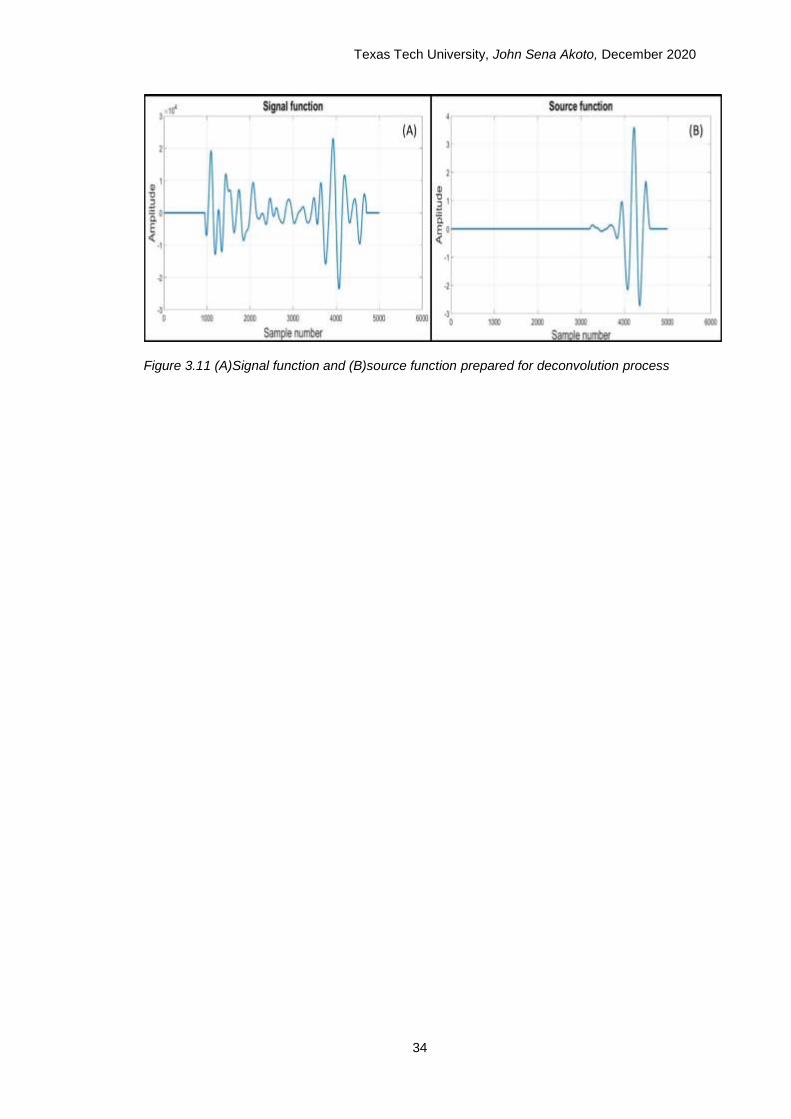
Figure 4.6 Colorshading plot for longitude 173°E. 410 km discontinuity seen as a positive amplitude at ~410 km with an uptick in depth between latitude 50-55˚N. 520 km discontinuity partially visible, becomes stronger after latitude 55˚N ................................................................................................... 48
Figure 4.7 Top: Wiggle plot from common stack longitude 196.5°E. Bottom: Wiggle plot from individual stack longitude 196.5°E. 410 km discontinuity seen as a yellow peak at ~410 km. Shallowing of 410 horizon between latitude 50-55˚N (Yellow: peak, Blue: trough). ............................................... 49
Figure 4.8 Colorshading plot for longitude 196.5°E. 410 km discontinuity seen as a positive amplitude at ~410 km with an uptick in depth between latitude 50-55˚N. ......................................................................................................... 50
Figure 4.9 Top: Wiggle plot from common stack longitude 193°E. Bottom: Wiggle plot from individual stack longitude 193°E. 410 km discontinuity seen as a yellow peak at ~410 km. Shallowing of 410 horizon between latitude 50-55˚N. 660 km discontinuity seen as a yellow peak at ~ 660km. 520 km discontinuity visible after latitude 55˚N. (Yellow: peak, Blue: trough) ...... 52
Figure 4.10 Colorshading plot for longitude 193°E. 410 km discontinuity seen as a positive amplitude at ~410 km with an uptick in depth between latitude 50-55˚N. 660 km discontinuity seen as a positive amplitude at ~660 km with a decrease in depth between latitude 50-55˚N. 520 km discontinuity visible after latitude 55˚N. .............................................................................. 53
Figure 4.11 Top: Wiggle plot from common stack longitude 172.5°E. Bottom: Wiggle plot from individual stack longitude 172.5°E. 410 km discontinuity seen as a yellow peak at ~410 km. Shallowing of 410 horizon between latitude 50-55˚N. 660 km discontinuity seen as a yellow peak at ~ 660km (Yellow: peak, Blue: trough). .......................................................................... 55
Figure 4.12 Colorshading plot for longitude 172.5°E. 410 km discontinuity seen as a positive amplitude at ~410 km with an uptick in depth between latitude 50-55˚N. 660 km discontinuity seen as a positive amplitude at ~660 km with a decrease in depth between latitude 50-55˚N....................................... 56
Figure 4.13 Top: Wiggle plot from common stack longitude 203°E. Bottom: Wiggle plot from individual stack longitude 203°E. 410 km discontinuity seen as a yellow peak at ~410 km. Shallowing of 410 horizon between latitude 50-55˚N. 660 km discontinuity seen as a yellow peak at ~ 660km (Yellow: peak, Blue: trough). .......................................................................... 57

Texas Tech University, John Sena Akoto, December 2020
ix
Figure 4.14 Colorshading plot for longitude 203°E. 410 km discontinuity seen as a positive amplitude at ~410 km with an uptick in depth between latitude 50-55˚N. 660 km discontinuity seen as a positive amplitude at ~660 km with a decrease in depth between latitude 50-55˚N....................................... 58
Figure 4.15 Topographic map of P410P. 410 km discontinuity shallows in the central portions and deepens in the NE and SW portions of the map. ...................... 60
Figure 4.16 P wave velocity model for 410. 410 km discontinuity exhibits high seismic velocity anomalies in the central region between latitude 50-60˚N signifying colder than average temperature mantle material. ............... 61
Figure 4.17 Topographic map of S410S. 410 km discontinuity generally shallows in the central portions and deepens in the NE and SW portions of the map. .... 62
Figure 4.18 S wave velocity model for 410. 410 km discontinuity exhibits high seismic velocity anomalies in the central region between latitude 50-60˚N signifying colder than average temperature mantle material. ............... 63
Figure 4.19 Topographic map S660S. Deep anomalies are observed between latitude 50-55˚N.............................................................................................. 64
Figure 4.20 S wave velocity model for 660. High-velocity anomalies can be seen between latitude 50-60˚N and in the NW corner of the map. High-velocity anomalies suggest colder than average mantle material. ............................. 65
Figure 4.21 P wave velocity model for 660. High-velocity anomalies can be seen between latitude 50-60˚N and in the NW corner of the map. High-velocity anomalies suggest colder than average mantle material. ............................. 65
Figure 4.22 Thickness model for Transition Zone shows thicker than average TZ thickness between latitude 50-55˚N ............................................................... 66
Figure 5.1 PP section across longitude 176˚E showing LAB and P220P. The 410 km discontinuity appears at ~410 km and shows a shallowing beneath 50˚N. ................................................................................................ 68
Figure 5.2 SS section across longitude 172.5˚E showing LAB. The 660 km discontinuity appears at ~660 km .................................................................. 68
Figure 5.3 (I) Topographic map of 410. (II) Velocity model of 410. ASZ (white dashed line) represents Aleutian subduction zone; A is a deepening anomaly that demarcates 410 beneath Bowers Ridge; B is a deepening anomaly that demarcates 410 beneath Alaska .............................................. 72
Figure 5.4 (I) Topographic map of 660. (II) Velocity model of 660. ASZ (white dashed line) represents Aleutian subduction zone; C and E are deepening anomalies that demarcates pooling of high-velocity slab material, colder than average slab material at 660; D demarcates 660 beneath Alaska .............................................................................................. 72
Figure 5.5 Thickness of transition zone. C and E show areas with thicker than average TZ where the subducting slab might be puddling and depressing the 660 significantly ..................................................................... 73
Figure 5.6 Depth map to 660 showing anomaly C and E, and profile lines AA’ (170°E), BB’ (185°E), DD’ (200°E), FF’ (42°N), and GG’ (50°N) ................... 74
Figure 5.7 Profile AA’ showing 520 km discontinuity and 660 km discontinuity deepening beyond latitude 50°N (anomaly E) ............................................... 75
Figure 5.8 Profile DD’ showing 660 deepening beneath latitude 45-50°N (anomaly E). 520 km discontinuity visible after latitude 55˚N. ....................................... 75
Figure 5.9 Profile GG’ showing section across anomaly C and E. 660 deepened to ~700 km. ........................................................................................................ 76
Figure 5.10 Control profile FF’, the 660 is observed at the expected depth of ~660 km. ................................................................................................................. 76

Texas Tech University, John Sena Akoto, December 2020
x
Figure 5.11 (A) Variation of 660 observed in profile AA’. (B)Enlargement of the dashed box around the 660 in profile AA’. The 660 is deepened by up to ~30km. ........................................................................................................... 77
Figure 5.12 (A) Variation of 660 observed in profile BB’. (B) Enlargement of the dashed box around the 660 in profile BB’. 660 here is relatively flat with a maximum deepening of 10 km. ................................................................... 77
Figure 5.13 (A) Absolute velocity profile for longitude DD’. (B) Enlargement of the dashed box showing 410, 520, and 660. Deepening of the 660 is observed along with a velocity reversal (II) of the 660. The 520 (I) visible after latitude 60°N. (C) Enlargement of the dashed box around the 660 to show ~30 deepening on the 660 km discontinuity ..................................... 78
Figure 5.14 (A) Absolute velocity profile for latitude GG’. (B) Enlargement of the dashed box showing high velocity on top of the 660 beneath anomaly C and E. ............................................................................................................. 79
Figure 5.15 S-Wave velocity perturbation profile AA’. High-velocity anomalies are observed between latitude 50-55°N (anomaly C). The deepening of the 660 is noticed between latitude 50-65°N. ...................................................... 80
Figure 5.16 S-Wave velocity perturbation profile DD’. High-velocity anomalies are observed between latitude 50-60°N (anomaly C). The deepening of the 660 is noticed between latitude 50-60°N. The 520 km discontinuity is visible beyond latitude 60°N. .......................................................................... 80
Figure 5.17 S-Wave velocity perturbation profile GG’. The TZ in profile GG’ (across anomaly C and E) is generally of high velocity suggesting a cold TZ ........... 81
Figure 6.1 Cartoon model of Pacific plate subduction beneath the Aleutian subduction zone across profile HH’. Shows elevated 410, 520, and deepened 660. Convective current and mantle chilling leads to sharp 520. Slab dehydration contributes to ~30km deepening observed on the 660, and possible slab rollback on the 660 accounts for cold anomaly seen beneath the ASZ at lower latitude. ........................................................ 83

Texas Tech University, John Sena Akoto, December 2020
1
CHAPTER I
INTRODUCTION
1.1 Background
The Aleutian subduction zone is an approximately 4,000 km long convergent plate boundary
that extends from Russia in the east to Alaska in the west. This plate boundary is where the
oceanic Pacific Plate subducts beneath the North American Plate. Subduction rates vary east
to west from 7.5 cm/year to 5.1 cm/year [Brown et al., 2013]. Additionally, the dehydration of
the subducting slab led to the formation of the Aleutian Island Arc, which is a volcanic arc
north of the subduction zone. The subduction zone is also a site for several earthquakes,
including the Good Friday Earthquake that recorded a magnitude of 9.2 on the Richter scale.
The Aleutian subduction zone falls within the Pacific Region, which is a densely sampled
region for PdP/SdS midpoints. A combination of all these features makes the Aleutian
subduction zone an interesting site for study.
Beneath the Aleutian subduction zone, the subducting Pacific Plate interacts with
discontinuities in the upper mantle transition zone (TZ). The transition zone includes three mid
mantle discontinuities at nominal depths of 660km, 520km, and 410km. The interaction of the
Pacific Plate with the 410, 520, and 660 km discontinuities is especially of great interest since
the response of the mid mantle discontinuities to a subducting slab helps reveal the kind of
phase and chemical changes at these discontinuities [Helffrich, 2000]. The prevailing theory is
that the discontinuities in the TZ are the result of phase changes in the olivine system. If this
is the case, the phase changes associated with the 410 and 520 results in an increase in
density and, as a result, enhances convection. However, the phase change at the 660 results
in a decrease in density for down going material, in which case it inhibits convection. Since
subduction zones are essentially downward convection of a cold slab, it makes a good place
to study the nature of these discontinuities and how they affect mantle convection.
The Aleutian subduction zone lacks a dense network of seismic stations that limits seismic
imaging techniques. PdP and SdS methods image boundaries by underside reflections, so

Texas Tech University, John Sena Akoto, December 2020
2
they are ideal for imaging regions with poor station coverage. The Aleutian subduction zone is
in a location surrounded by earthquakes from the richest source region on Earth, the west
Pacific ring of fire, that are recorded by the densest seismic network available, the US
transportable array; as a result, there is abundant data for this project. Using PdP and SdS
seismic phases, we will image the upper mantle transition zone to better understand its
properties by determining how it is affected by the subducting Pacific Plate.
1.2 Purpose and Objectives of the Study
The study aimed to investigate the deep structure of the Aleutian subduction zone using
bounce-point PdP and SdS seismic phases. PdP and SdS bounce-point waves allow us to
study areas with a sparse network of seismic recording stations. Moreover, results from this
research will shed more understanding of the upper mantle TZ and how the descending slab
interacts with it. The specific objectives of this project are:
1. Investigate the TZ beneath the Aleutian subduction zone by mapping the depths of
the 410km, 520km, and 660km discontinuities.
2. Explain the mantle dynamics between the subducting slab and the mantle
discontinuities.
3. Investigate the origin of Bowers Ridge

Texas Tech University, John Sena Akoto, December 2020
3
CHAPTER II
LITERATURE REVIEW
2.1 Aleutian-Bering Sea Region
The tectonically active Aleutian-Bering sea region is bounded on the south by the Aleutian
Subduction zone, where the Pacific plate subducts beneath the North American plate. The
Bowers and Shirshov ridge are postulated to be island arcs resulting from plate subduction
[Ben-Avraham and Cooper, 1981; D. W. Scholl, 1975]. Additional geologic structures of
tectonic importance include Bering continental margin, Emperor seamounts, Umnak plateau,
and Kamchatka (Commander), Aleutian, and Bowers Basin [Verzhbitsky et al., 2007].
Figure 2.1 Geologic features present in the Aleutian-Bering Sea Region (Based Wikipedia File: Hawaii hotspot.jpg, which was initially generated by National Geophysical Data Center/USGS as published at http://www.ngdc.noaa.gov/mgg/image/2minrelief.html).
The Shirshov ridge is found on the western part of the Aleutian arc. The Bowers ridge loops
north from the Aleutian ridge and extends about 900 km northwest, terminating at the
Shirshov ridge. The Shirshov ridge extends 750 km southward from the Siberian mainland
and borders against the Aleutian arc. In combination, these three ridges cordon the Bering
Sea region into three basins, namely Bowers, Kamchatka (Commander), and Aleutian basin.
Seismic refraction and reflection investigations showed that the Aleutian basin is by far the
largest of the three basins [D. W. Scholl, 1975]. This basin is underlain by approximately 3 km
of semi consolidated sedimentary rock, with seismic velocities ranging from 2.1 to 2.9 km/s.

Texas Tech University, John Sena Akoto, December 2020
4
Beneath this semi consolidated rock is a 1 to 6 km layer of lithified sedimentary (or in part
volcanic) rock characterized by seismic velocities ranging from 3.2 to 4.3 km/s. The Bowers
basin also has similar stratification as the Aleutian basin, the difference being that its
sedimentary fill is slightly thinner and directly overlies a thick rock unit of about 5.8 to 6.2
km/s. Ludwig and others have shown that this thick rock unit makes up most of the internal
bulk of the Aleutian and Bowers ridge [Ludwig, 1971]. The Kamchatka basin, which is also
known as the Commander basin, is underlain by 1 to 2 km of semi consolidated deposits
overlying a lower lithified layer of sedimentary rock characterized by seismic velocities of
about 3 km/s. However, due to sparse data, the stratigraphy of the Kamchatka basin is not
known in as much detail as the Aleutian and Bowers basin.
The Bering Continental Margin is a 1,300 km long broad arc, which extends from Kamchatka
to the tip of the Alaska Peninsula. Topographically, the margin separates the Bering Sea and
the Aleutian Basin. The margin is divided into three geomorphic provinces: (1) the flat outer
Bering shelf; (2) the steep Bering continental slope; (3) the deeper and more gently seaward
sloping continental rise. Lithologically, the margin is comprised of two main structural units:
(1) an acoustic basement, made up of lithified rock, and (2) a 1-1.5 km thick overlying
stratified section of semi consolidated sedimentary rock and unconsolidated sediments. The
stratified layer is further divided into three units; a main layered sequence, a rise unit and a
surface-mantling unit [Scholl et al., 1968]
2.1.1 Aleutian Subduction Zone
The Aleutian subduction zone is a ~2500-mile-long convergence boundary where the Pacific
Plate collides and subducts beneath the North American plate at an average rate of 6.3 cm/yr.
It extends from the Alaska Range to the Kamchatka Peninsula [D. W. Scholl, 1975]. The
Aleutian subduction zone is made up of the Aleutian Trench and the Aleutian arc.
The Aleutian trench is a steep and deep V-shaped depression that forms between two
converging plates as the oceanic slab subducts. The trench extends along the southern
coastline of Alaska and the Aleutian island arcs for 3400 km. The island arc forms from
volcanic eruptions from the dehydration of the subducting slab at ~100 km depth.

Texas Tech University, John Sena Akoto, December 2020
5
The Aleutian island arc was formed ~50-55 Mya as a result of the subduction of the Kula plate
beneath the North American Plate prior to the subduction of the Pacific plate [Steven
Holbrook et al., 1999]. The island arc formed in 4 phases: the initial phase, the early phase,
the middle phase, and the final phase. The initial phase of arc development began from the
Late Mesozoic to earliest Tertiary, during which the bulk of the arc formed rapidly by mafic
submarine volcanism and plutonism. In the early phase (Eocene to middle Miocene),
volcanism on the arc declined, and tectonically elevated volcanic terranes were sub-aerially
eroded. The early phase was followed by the middle phase (middle Miocene to middle
Pliocene), a period of plutonization and upliftment, which resulted in more erosion of the arc.
During the final phase (middle Pliocene to present), an extensional rifted arc was overlain by
post-orogenic deposits and crested by a chain of andesitic stratovolcanoes [D. W. Scholl,
1975].
2.1.2 Bowers Ridge
The Bowers Ridge is located in the Aleutian Basin. It is an arcuate feature connected to the
Aleutian ridge on the south and extends to the Shirshov ridge on the north; it spans a total
length of 900 km [Verzhbitsky et al., 2007]. The origin of Bowers Ridge is still heavily debated,
with several different hypotheses being proposed.

Texas Tech University, John Sena Akoto, December 2020
6
Figure 2.2 Map of the Bering Sea showing the three main rises; Bowers Ridge, Umnak Plateau, and Shirshov Ridge. Profile AB intersects Shirshov Ridge, profile CD intersects Bowers Ridge, and profile EF, Umnak Plateau. These profiles show gravity, magnetic, and seismic character of the geologic feature they cross [Ben-Avraham and Cooper, 1981]
Some of the hypotheses are that the ridge is an ancient, remnant island arc outgrowth of the
Aleutian Ridge and a microcontinent [Kienle, 1971], [Karig, 1972], [Nur and Ben-Avraham,
1978]. Proponents of the hypothesis that Bowers Ridge is older than the Aleutian ridge also
suggest that it was not formed in-situ. Instead, it came to its present location by a more former
plate, possibly the northwards-moving Kula plate, prior to the formation of the Aleutian ridge.
Several models have been developed to support their claim.
One model proposes that prior to the formation of the Aleutian ridge, the subduction zone was
more northwards around the Bering Sea margin, where the Bowers Ridge and Umnak
Plateau were proto structures on the northward bound subducting Kula plate. In this model,
there was also a long, north-trending transform fault west of the Bowers Ridge. As Kula plate
moved north and subducted beneath a more northerly trench, it resulted in the Bowers Ridge
and Umnak Plateau colliding with the southern edge of the Bering Sea margin. This collision
caused the subduction zone to jump southward to the location of the current Aleutian Ridge. It
Texas Tech University, John Sena Akoto, December 2020
7
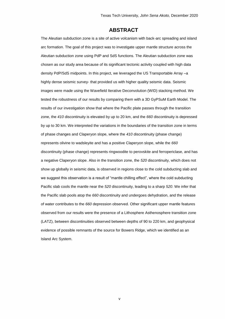
is claimed that this collision event took place by the late Mesozoic or early Tertiary based on
the positions of the Umnak Plateau and the Bowers Ridge [Ben-Avraham and Cooper, 1981].
Figure 2.3 Formation model 1 of the Bowers Ridge, Umnak Plateau, Shirshov Ridge, and Aleutian Ridge A. late Mesozoic; B. early Tertiary. Prior to the formation of the Aleutian subduction zone, the Shirshov ridge, Bowers ridge, and Umnak plateau were driven by plate motion and collided into the Bering shelf. [Ben-Avraham and Cooper, 1981]
A second model by Ben-Avraham and Cooper, 1981 hypothesizes that the Shirshov Ridge,
Umnak Plateau, and the Bowers Ridge were all parts of a large arc structure located east of
the Kamchatka Peninsula. A north-trending spreading ridge is thought to have also existed at
the same time in the area where the present Bering Sea is located [Hilde et al., 1977]. A
series of east-west trending transform faults separated the three proto structures. The pull
from the subduction zone at the Bering Sea margin causes the spreading ridge to eventually

Texas Tech University, John Sena Akoto, December 2020
8
caused the Shirshov Ridge, Bowers Ridge, and Umnak Plateau to collide into the Bering Sea
margin. As a result, just like in the prior model, the subduction zone shifted southerly to its
present location at the Aleutian Ridge. Magnetic investigations by Cooper and others (1976)
support this hypothesis since they observed that the magnetic anomalies became older west
of the subducted spreading ridge.
Figure 2.4 Formation model 2 of the Bowers Ridge, Umnak Plateau, Shirshov Ridge, and Aleutian Ridge. A. and B. is late Mesozoic; C. early Tertiary. (A) shows the Bowers ridge, Umnak plateau, and the Shirshov ridge in their original location. (B) shows the Bowers ridge, Umnak plateau, and the Shirshov ridge transported by seafloor spreading. (C) shows the Bowers ridge, Umnak plateau, and the Shirshov ridge in their current location. [Ben-Avraham and Cooper, 1981]
2.2 Transition Zone
2.2.1 Introduction
The transition zone (TZ) was described by [Bullen, 1986] as a diffuse region of high seismic
wave-speed gradient extending from 410 to 1000 km. In his model, he classified the transition

Texas Tech University, John Sena Akoto, December 2020
9
zone as Region C with the lower mantle as Region D (figure 2.5). [Birch, 1952] was the first to
suggest discontinuities were caused by polymorphic phase changes. He hypothesized that
the Repetti discontinuity at ~1,000 km marked the top of the lower mantle and that high
seismic wave-velocity gradients are caused by phase changes.
Figure 2.5 Model showing a cross-section of the Earth with the different layers [Bullen, 1986]
[Gutenberg, 1959] proposed early models of the transition region with high wave-speed
gradients without abrupt discontinuities. It was not until the 1960s that sharp jumps in seismic
velocity were discovered at depths of approximately 400 and 650 km. After the initial
discovery of the transition zone discontinuities, several investigators used a variety of
methods to confirm the existence of the 410 and 660 km discontinuities. These discontinuities
defined the boundaries of the transition zone.
Thermodynamic considerations were used to debate that the transition zone discontinuities
are caused by sharp phase changes of olivine to spinel, and then to post-spinel, rather than
chemical changes. They showed that the 410 km discontinuity has a positive Clapeyron
slope, and the deeper 660 has a negative Clapeyron slope [Anderson, 2007]. This means that

Texas Tech University, John Sena Akoto, December 2020
10
a cold subducting slab of the same composition as the surrounding mantle will shift the 410
up, enforcing vertical motion in the subducting plate. On the contrary, the cold subducting slab
would depress the 660 km discontinuity, hindering vertical downward movement until the
plate has warmed up to a denser phase. Alternatively, hot rising magma plumes of similar
composition as the mantle will elevate the 660 and depress the 410 km discontinuity.
The TZ is a layer of Earth’s mantle and is located between the upper mantle and the lower
mantle. Thermodynamic considerations have been used to argue that the 410 and 660 km
discontinuities are phase changes caused by pressure-induced changes of crystal structure in
minerals derived from olivine [Anderson, 2007]. Also, based on thermodynamic equilibrium,
the depths of these discontinuities vary depending on temperature and composition. The
depths will, therefore, vary significantly in locations of subducting lithospheric slabs and hot
mantle plumes due to the significant temperature anomalies associated with these features.
To better understand the phase changes associates with discontinuities of the TZ, laboratory
experiments reproduced the temperatures and pressures corresponding to depths up to
750km were performed on olivine, the most abundant mineral in the mantle. At pressures and
temperatures consistent with the 410 km depth, it was observed that α-olivine transformed
into β-spinel. β -spinel (wadsleyite) then changes into γ-spinel at conditions corresponding to
those associated with depths of about 520 km. Indeed, a discontinuity at 520 km has been
reported; however, studies have shown that velocity contrast is too small and gradational
across this discontinuity to produce observable P520P or S520S phases under nominal
mantle conditions. At 660 km pressure, γ-spinel (ringwoodite) transforms into perovskite and
magnesio-wüstite. Recent studies using multi anvil apparatus have shown that, at 660 km
pressures and significantly higher temperatures of 2100-200℃, there exists a post-garnet
phase change that transforms garnet to bridgmanite that would occur at temperature and
pressures consistent with depths of 720 km [Ishii et al., 2018].
The135 Earth Model (figure 2.6) shows the P and S wave velocities as a function of depth
from 200 km to 800 km. In addition, the volume fraction of the primary mantle constituents

Texas Tech University, John Sena Akoto, December 2020
11
and how they vary with respect to depth are shown on the right. We can observe a sharp
increase in both P and S waves at the 410 and 660 km discontinuities. We can also find from
the volume fractions the phase changes that occur through the transition zone. Between
200km to 660 km, olivine comprises approximately 60% of the volume fraction, with phase
transitions from olivine to wadsleyite occurring at 410 km, wadsleyite to ringwoodite at 520
km, and ringwoodite to perovskite and ferropericlase around 660 km. Pyroxene and garnet
make up the remaining 40% [Q Cao et al., 2011].
Even though there appears to be a lot of information about the transition zone, the detailed
structure of this region is still mostly controversial, and it remains a subject of investigation.
Figure 2.6 Phase diagrams for pyrolitic mantle composition. (A) Left, P- and S wave speed (and mass density ρ) as a function of depth and pressure in Earth’s mantle. Right: Volume fraction of mantle constituents between 200-800km. The green line depicts 410 phase change; the blue line shows 520 phase change, and the red line represents 660 phase change [Q Cao et al., 2011] [Kennett et al., 1995].

Texas Tech University, John Sena Akoto, December 2020
12
2.2.2 The Mantle transition zone controversy
There is an ongoing debate in geochemical literature about whether the 650 or 1000 km
discontinuity is the interface between the upper and lower mantle and whether there are
chemical changes deeper than the 1000 km depth. Currently, geochemical investigations and
convection simulations assume that the 650 km phase change separates the “depleted
convecting upper mantle” from the “primordial undegassed lower mantle.” Geodynamic
modeling suggests that if the 650 km is not a chemical change, then there can be no deeper
chemical change, which in turn implies that the mantle is chemically homogenous. The
transition zone thus holds the key to whether there is whole-mantle or layered-mantle
convection [Anderson, 2007].
2.2.3 Variations in Discontinuity Depths
Cold subducting slabs have been shown to warp the 410 km discontinuity to shallower depths
by about 8 km per 100 K, and depress the 660 km discontinuity down by about 5 km per 100
K (shown in figure 2.7c) [Bina and Helffrich, 1994]. Conversely, unusually high temperatures
will depress the 410 km and elevate the 660 km discontinuity. As a result, the TZ is expected
to thicken by a maximum of about 13 km per 100 K, where temperatures are cold and thin by
a similar amount where temperatures are high (assuming depth anomalies extend across the
TZ) [Bina and Helffrich, 1994]. Anomalous temperatures vary the depth of the 410 and 660 as
a response to their respective Claperyon slopes. The 410 phase change has a positive
Claperyon slope, and as a result, increasing mantle temperature increases the depth of the
410 km discontinuity. On the other hand, the 660 has a negative Claperyon slope, causing the
660 depth to decrease with increasing temperature (shown in figure2.7 C). Aside from cold
subducting slabs and hot mantle plumes can create lateral variations in mantle temperatures
in excess of 200 K that can cause anti-correlated shallowing and deepening of the TZ
discontinuities that can result in thinning or thickening of the TZ of 20-35 km because of anti-
correlated deflections in both discontinuities [Cordery et al., 1997].

Texas Tech University, John Sena Akoto, December 2020
13
Figure 2.7 A.Effects of a cold subducting slab on the 410 and 660 km discontinuities; B.Effects of a hot mantle plume on the 410 and 660 km discontinuities; C Green line shows olivine to wadsleyite phase (positive Claperyon slope), orange ringwoodite to perovskite and ferropericlase (post-spinel with negative Claperyon slope) and blue majorite to magnesium perovskite (positive Claperyon slope). 1 is cold geotherm, 2 is average geotherm, 3 is warm geotherm, 4 is anomalously warm geotherm. D Hot upwellings showing post-garnet phase. E Subducting slab[Q Cao et al., 2011]

Texas Tech University, John Sena Akoto, December 2020
14
Variations in mantle chemistry also affect the depths and sharpness of the transition zone
discontinuities. High FeO content decreases the depths of the discontinuities and generally
thickens the TZ [G. R. Foulger, 2004]. In addition, studies have shown that water content
increases the sharpness of the 410 km discontinuity [A Cao and Levander, 2010; Mohamed
et al., 2014].
Global investigations have revealed that the average thickness of the transition zone is ~ 242
km[Flanagan and Shearer, 1998]. For example, researchers discovered the thinnest transition
zone, which is 181 km thick beneath Sumatra. Enigmatically, this region also appears to have
a thick accumulation of cold slabs at the base of the TZ, which is expected to thicken the
transition zone. In the western USA, the thickness of the transition zone varies from 220 to
270 km, which suggests a relief of 20 to 30 km on each discontinuity. However, there is no
corresponding surface geology, topography, or plate tectonics to explain the thickening
[Anderson, 2007]. In conclusion, there is a lot to understand about the variation in the
thickness of the transition zone. The transition zone remains a critical region for investigation
since it can help explain how the mantle convects.
2.2.4 Transition Zone Water Filter
The transition zone is considered a water filter because water-bearing minerals are removed
from wet subducting slabs through a slab dehydration process within the TZ [Bercovici and
Karato, 2003; Richard et al., 2006]. Additionally, studies have shown that the transition zone
(the upper mantle between 410 and 660 km) serves as a water reservoir with water occupying
approximately 0.1wt% of the mantle [Bercovici and Karato, 2003]. The transition zone is able
to store water filtered out from the wet subduction slab because of its composition of high
solubility and diffusivity minerals. For example, wadsleyite and ringwoodite (both transition
zone minerals) exhibit high water solubility of 2.4 weight percentage and 2.7 weight
percentage giving them the ability to store water. Thus, wet slabs that stagnate in the
transition zone typically undergo dehydration by expelling water in dense hydrous magnesium
silicates (DHMS) [Richard et al., 2006]. This process of slab dehydration releases water,
which shallows the 410 and deepens the 660, essentially thickening the transition zone[Bina
and Helffrich, 1994].

Texas Tech University, John Sena Akoto, December 2020
15
2.3 PdP and SdS Precursor Function
PP and SS body waves also known as underside bounce-point reflections are from the
midpoint between an earthquake source and a seismic receiver. PdP or SdS phases travel
similar trajectories to the PP and SS phases, but instead of traveling to the surface, they
reflect at a discontinuity at a depth “d” below the surface. PdP and SdS phases are referred to
as precursors because they travel a shorter time than the PP or SS and, as a result, arrive
earlier (figure2.8 and figure2.9). For example, P410P is the precursor that reflects off the
underside of the 410 km discontinuity.
Figure 2.8 PdP wave path and its precursor P660P reflected on the underside of the 660km discontinuity. Star and red triangle represent the source and receiver, respectively. The red path indicates the PP wave path, and the blue path indicates the P660P wave.

Texas Tech University, John Sena Akoto, December 2020
16
Figure 2.9 Seismic records for two stations in a study by [Deuss, 2009] shown with solid lines compared to synthetics based on the PREM model shown in dashed lines. The 660, 410, and 220km discontinuities are detected as precursors to the SdS.
PdP and SdS phases are often used to study the mantle of the earth, precisely the existence,
and characteristics of discontinuities within the transition zone (410, 520, and 660
discontinuities). PdP and SdS waves have an advantage over other seismic phases because
they provide significant coverage in both oceanic and continental regions, regardless of the
density of seismic recording networks in those regions [Chambers et al., 2005; Deuss, 2009;
Flanagan and Shearer, 1998; Helffrich, 2000; Lawrence and Shearer, 2006; Ritsema et al.,
2002; Schäfer et al., 2009]. Bounce-point data is ideal for studying regions in the North Pacific
and South Pacific, such as Alaska, Aleutian Trench, Chinook Trough, Hawaii Islands, etc.
where there is a paucity of seismic stations. Owing to the central and northern Pacific being
surrounded by seismically active subduction zones, and very dense seismic networks in East
Asia, and North America (particularly the very dense US transportable array), they are the
best-illuminated region in the world by PdP and SdS phases (figure2.10B).

Texas Tech University, John Sena Akoto, December 2020
17
Figure 2.10 A. Global map showing seismic sources in black and receivers in red. B. Bounce-points are shown as black dots in figure 2.12 B.
B
A

Texas Tech University, John Sena Akoto, December 2020
18
2.4 Studies Investigating the TZ
2.4.1 Topography of the “410” and “660” km seismic discontinuities in the Izu-Bonin subduction zone [Collier and Helffrich, 1997]
The focus of this investigation was to better understand the effects of a subducting slab on
the “410” and “660” km mantle discontinuities in the Izu-Bonin region in the western Pacific.
The study aimed at showing that these discontinuities are because of thermodynamic phase
transformation rather than chemical compositional change. To prove this, they hypothesized
that, “A compositional boundary should be largely indifferent to a temperature change
whereas the thermodynamic properties of a phase transformation prescribe elevation or
depression of the discontinuity depending on the sign and magnitude of the ‘Clapeyron
slope.’”
To perform their investigation, [Collier and Helffrich, 1997]used topside S-to-P discontinuity
conversions and underside discontinuity reflections collected from networks of vertical
seismometers in the United Kingdom and the northwestern United States. They analyzed
data collected from 21 earthquakes with depths between 40 and 548 km and magnitudes
between 5.4 and 6.4. The combination of array data from the UK and the US allowed
interrogation of the discontinuities from both sides of the slab.
Figure 2.11 Map illustrating source from Izu-Bonin and receivers in the United Kingdom and Pacific North-West seismic networks. Great circle paths of the seismic waves are shown in solid lines, and plate boundaries are shown in dashed lines [NUVEL-1, 1990].
The results of the study showed an anti-correlation between the “440” and “660” expected for
a phase change origin of both discontinuities with Claperyon slopes of opposite signs. They

Texas Tech University, John Sena Akoto, December 2020
19
also found that the “410” was elevated by about 60 km, and the “660” was depressed by 40
km in similar regions. They estimated that the temperature of the slab interior was 600±75℃ at
a depth of 350 km. They also tentatively suggested a broader 410 discontinuity in the interior
of the slab.
2.4.2 Seismic Imaging of Transition Zone Discontinuities Suggest Hot Mantle West of Hawaii [Q Cao et al., 2011]
The object of this study was to constrain the thermal plume beneath Hawaii as well as its
effects on the transition zone discontinuities. The research suggests that molten material
does not rise directly from the lower mantle through a narrow vertical plume beneath Hawaii.
Instead, the study proposes that the plume accumulates near the base of the transition zone
before being channeled in a flow toward Hawaii and other islands.
In this study, [Q Cao et al., 2011] uses underside reflections (SdS), which arrive as precursors
to surface-reflected SdS waves at sensors far from the study region. In their investigation,
three-dimensional (3D) inverse scattering of SdS wavefield is combined with a method known
as generalized Radon transform to process the SdS data. This unique processing flow avoids
the problem of low spatial resolution, which typically plagues the conventional method of
stacking specular (mirror-like) SdS reflections across large (10° to 20° wide) geographical
bins. They imaged the transition zone beneath Hawaii with approximately 170,000 broadband
records of the SdS wavefield. They analyzed seismic data recorded by ~2250 seismographic
stations around the Pacific. From ~ 4800 earthquakes with depths greater than 75km and
magnitudes greater than 5.2. They had relatively good data coverage across their study area,
with an exception in the southwest region.

Texas Tech University, John Sena Akoto, December 2020
20
Figure 2.12 Left: (Top) Map of study area showing the geographical distribution of ~170,000 surface mid-points of SdS waves –the darker shaded regions have denser coverage; (bottom) trajectory of underside reflections at the surface (SS) and at mantle discontinuities (SdS); precursor stack showing signal associated with S660S, S410S, and SdS waves [after (27)]. Right: (Top) Distribution of ~4800 sources (red symbols) and ~2250 receivers (blue); (bottom) diagram of SdS, S410S, and S660S trajectory [Q Cao et al., 2011]
After processing the data, a cross-section was taken across the 3D image volume. The cross-
section can be seen in the plan view in figure 2.14. From the cross-section, they were able to
track the “410”, “520”, and “660”. The “660” in the region I (below and east of Hawaii) is
slightly shallower than the global average (~650 km). In region II (between Hawaii and 165°
W), the “660” is more anomalous (~640 km). Between 167° and 179°W (region III), the “410”
reaches 430 km, and the “660” appears anomalously deep (~700 km).
Figure 2.13 Cross-section across Hawaii. (A) Seismic image overlaid on tomographically inferred wave-speed variation. (B) Enlarged figure between 370 and 760 km, green dashes are interpreted as 410, blue dashed line as 520, and red dashed line as 660 [Q Cao et al., 2011].

Texas Tech University, John Sena Akoto, December 2020
21
In figure 2.14 it is observed that the transition zone is relatively thin beneath Hawaii and thick
on the west of Hawaii (region III). In addition, the correlation between 410 and 660 depth
variations is negatively correlated beneath Hawaii, but conspicuously positive correlated in
region III.
Figure 2.14 (A) Topographic map of 410 and (B) Topographic map of 660. The thick black line is the E-W cross-section in Figure.2.13 (C) Isopach between 410 and 660. (D) Correlation between 410 and 660 [Q Cao et al., 2011]
From their observations, they concluded that the up doming of the “660” beneath region II is
consistent with the post-spinel transition in hot mantle regions. While the deepening of the
“660” beneath region III was enigmatic to the post-spinel transition, it was interpreted as the

Texas Tech University, John Sena Akoto, December 2020
22
post-garnet transition caused by a temperature anomaly at that depth. No defined pathways
of flow from the deep anomaly to the Earth’s surface were resolved. However, the study
suggests that Hawaii's volcanism might stem from the temperature anomaly in region III.
Figure 2.15 Schematic model of transition zone beneath Hawaii. Green, blue, and red lines represent 410, 520, and 660, respectively. Dashed arrows show the movement of hot mantle plume within the transition zone [Q Cao et al., 2011]

Texas Tech University, John Sena Akoto, December 2020
23
CHAPTER III
METHODOLOGY
The focus of the study was to investigate the crust and mantle beneath the Aleutian
subduction zone by using PdP and SdS data. As we established earlier, the use of PdP and
SdS data are advantageous to the study of the mantle of areas that lack dense networks of
seismic stations such as the Aleutian subduction zone. Discontinuities can be imaged by
leveraging the differences in the arrival times between the PP/SS phase that reflects off the
surface and the PdP /SdS phase that reflects off mantle discontinuities.
The bounce-point data were obtained from the IRIS Data Management Center, a repository of
seismic data. After downloading, the data were screened and prepared for the analyses that
we run.

Texas Tech University, John Sena Akoto, December 2020
24
Figure 3.1 Flowchart of methodology, shows a summary of the procedure employed in this study
3.1 Data Collection and Preparation
All data for this study were acquired from the IRIS Data Management Center. For this study,
we downloaded PdP and SdS data collected for earthquakes of magnitude 5.8 and larger
between January 1990 to November 2018 for every broadband seismic station in the DMC
catalog. We hoped this will give sufficient redundancy of data, thus reducing the effect of few
noisy seismic records on our overall dataset. We downloaded data with a great circle of 60-
180° between station and event.

Texas Tech University, John Sena Akoto, December 2020
25
The first step in data preparation was sorting; a sorting technique was done to organize the
data by the station. Next, the sorted data were cut to isolate the seismic phases relevant to
our study. This recording contains all the seismic phases P, S, PcP, PcS, and other phases
as well as the PdP and SdS phases. To isolate the P, S, PdP, and SdS phases, time windows
were selected to allow for precursor information down to 1000km (120 seconds before the
first P arrival to 1800 seconds after the first P arrival).
After the data was sorted and cut, the next steps were to detrend, taper, and filter these data.
The purpose of the aforementioned procedures was to enhance the signal to noise ratio of the
seismic recordings. The data were detrended by fitting a line to the time series and removing
the line from the data. For stable deconvolution and cross-correlation, it is crucial for the data
stream to begin and end with zeros, so we apply a linear taper to each end of these data.
Broadband high gain data obtained from IRIS DMC typically have sampling rates of 20, 40, or
50 samples per second (SPS), depending on the local network and the year that the data
were collected. To use these data, we had to resample all the data to a uniform sampling rate.
For the study, we resampled all our seismic recordings to 10 sps. After tapering, the data was
filtered using a phaseless Gaussian filter. An anti-aliasing low pass filtered was applied to
these data to enable us to decimate it to 10 samples per second, thereby saving on disc
space and speed processing. Low pass filtering does not harm these data because there is
generally no teleseismic signal at frequencies above 1 Hz, and so high-frequency noise tends
to be local noise. To remove low-frequency noise, usually related to station instability, a 0.05
Hz high pass filtered was applied.

Texas Tech University, John Sena Akoto, December 2020
26
Figure 3.2 Example of a raw seismic time series before filtering
Figure 3.3 Example of seismic data after filtering
The final step before processing was to quality check the data. This was performed in three
stages:
1. Preliminary scanning: a threshold signal to noise ratio of 2 was used to eliminate poor
seismic traces.
2. Detailed automated scanning was performed and based on great circle arc (to
eliminate data from a distance with interfering phases), peak signal to noise ratio, and
standard deviation signal to noise ratios- to discriminate the data into 3 groups (good,
borderline, and bad).

Texas Tech University, John Sena Akoto, December 2020
27
3. Detailed visual inspection: For this stage, we visually inspected all borderline traces
and used our judgment to either assign them to the good or bad class. The bad class
was eliminated.
After quality checking, 658000 PdP traces and 444000 SdS traces qualified to be processed
and used in the study.
3.2 Data Processing
3.2.1 Ocean Bottom Multiples Removal (Deoceaning)
Removal of Ocean Bottom Multiples has become a standard procedure in processing PdP
data [Ailiyasi Ainiwaer, 2014; Duncan, 2012; Rogers, 2013]. Throughout PdP data, there is
usually steady positive arrival of a higher frequency horizon, which arrives marginally earlier
than the PdP phase causing a double PdP peak. This horizon is frequently identified in
recordings from offshore stations and has been shown to be a product of the P wave
bouncing at the ocean bottom-seawater contact. This ocean bottom reflection added to the
regular sea-water-air PdP reflection causes double peaks observed in PdP data. Since the
PdP phase is used as the source in the deconvolution process, this double peak will be
carried on to all the precursors extracted from the signal, which is problematic. To avoid the
issue of precursors with double peaks, all PdP data recorded offshore are de-oceaned (ocean
bottom arrivals are removed) prior to deconvolution. Removing the double peak PdP involved,
first, finding all data recorded offshore, followed by deconvolving the double-peaked PdP from
itself and saving this data into the source channel. While this initial deconvolution causes
precursors to have double peaks, the two PdP impulses will collapse to a single PdP pulse.
The double-peaked precursors in the source channel are inconsequential since they will be
tapered off during source function creation [Duncan, 2012]. Ocean Bottom Multiple Removal
is not carried out on SdS data because S waves cannot travel in fluids, and do not exhibit
multiples due to seawater-air contact.

Texas Tech University, John Sena Akoto, December 2020
28
3.2.2 Ray Tracing
Raytracing and travel time calculation is a process of computing the travel time and distance
traveled by all possible PdP, SdS, PdP, and SdS phases from the surface to 700 km. The
travel times and depths calculated are interpolated based on a given velocity model. In our
study, we used the 1-D IASPI 91 velocity model[Kennett and Engdahl, 1991] to compute our
travel times and depths. A travel-time calculation program, which was written by [Duncan,
2012], was used to calculate the expected arrival times for PdP and SdS across the
teleseismic range (30° to 180°)
Figure 3.4 Example of a travel time curve for PdP and P410P (Blue: PdP, Red: P410P)

Texas Tech University, John Sena Akoto, December 2020
29
Figure 3.5 Travel time curve for PdP and P660P (Blue: PdP, Black: P660P)
3.2.3 Beamforming
The next step in processing the screened data is beamforming. Beamforming is a terminology
that refers to a wide array of geophysical processing techniques. However, in this study,
beamforming simply refers to time-shifting and stacking all seismic data from the same event
that falls within a specified search radius at the receiver end of the data. Stacking data from
the same event at the receiver end does one of two things depending on whether a small or
large stacking radius is chosen. When a small stacking radius is used to beamform, the stack
produced generally maintains its local phases (such as Moho phases) as well as local
lithosphere and mantle variations. This is because a few close traces from the same event
are stacked, resulting in a stack that amplifies local crustal and mantle variations common to
the traces in the radius. However, if a large stacking radius is used, the stack generally
averages out local phases, crustal and mantle variations, resulting in a trace that seems to
have traveled through a generally uniform crust and mantle.
In this study, several stacking radii were selected: 1°, 2°, 4°, 8°, 16°, 32°, and 360°. From
these stacking radii, 360° bin, which encompasses all traces of the same event from the
globe, was used as a clean PdP and SdS source. Signal to noise ratios in this bin was

Texas Tech University, John Sena Akoto, December 2020
30
maximized, and phases due to local variations were averaged out. For the signal, we varied
between the 1°, 2°, 4°, and 8° stacking bins. We noticed that the 4° bin consistently gave us
cleaner, high signal to noise ratios without compromising local variations. Thus, we settled on
the 4° bin for our signal.
Figure 3.6 Illustration of beamforming overview. Seismic records from the same event that falls within the beaming radius ‘r’ are cross-correlated, time-shifted, and stacked. The violet star represents the seismic event, and the orange circles represent seismic recordings from the event that fall within the specified stacking radius ‘r’.
Figure 3.7 Sample seismic recording (FD_4.5_PdP_US.KVTX.00.BHZ.M__at__2018-11-25T16.49.57.000Z) prior to beamforming.

Texas Tech University, John Sena Akoto, December 2020
31
Figure 3.8 Sample seismic recording (FD_4.5_PdP_US.KVTX.00.BHZ.M__at__2018-11-25T16.49.57.000Z 16) after a 16° beamforming
Figure 3.9 Sample seismic recording (FD_4.5_PdP_US.KVTX.00.BHZ.M__at__2018-11-25T16.49.57.000Z 16) after a 32° beamforming

Texas Tech University, John Sena Akoto, December 2020
32
Figure 3.10 Sample seismic recording (FD_4.5_PdP_US.KVTX.00.BHZ.M__at__2018-11-25T16.49.57.000Z 16) after a 360° beamforming
3.2.4 Deconvolution and Stacking
Convolution is simply an mathematical operator where a signal or data stream in time, s(t)
gets smeared into a response function, r(t). In the case of earthquake seismology, the signal
or data stream is a teleseismic shock from an earthquake, and the response function is the
discontinuities in the earth encountered by the traveling earthquake waves, technically known
as the earth response function. The result of this convolution of the earthquake signal with the
earth response function is recorded as a time series by the several seismographs deployed
worldwide, which is then studied by seismologists to understand the earth better. The import
of deconvolution in seismology is simply to reverse the process of convolution by extracting
the source mechanism (earthquake wave) from the recorded time series leaving behind the
earth response function, a function, which reveals characteristic seismic properties of various
discontinuities in the subsurface.
3.2.5 Single Iterative Deconvolution
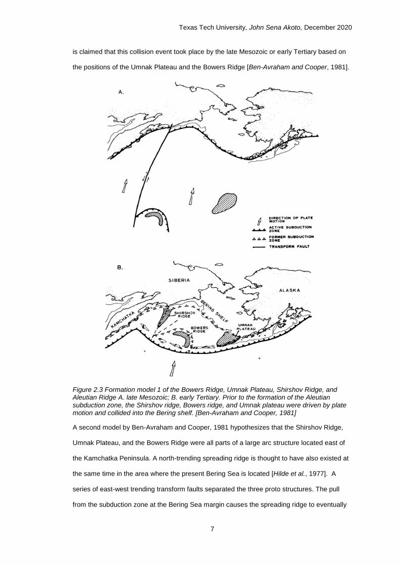
In a single-event iterative deconvolution, one of the channels from the beamed PdP/SdS data,
preferably a large radius channel, is used as the source function. The signal function is
prepared from a second channel from the beamed data, in this case giving preference to

Texas Tech University, John Sena Akoto, December 2020
33
smaller radius channels. A taper is applied to the source function to zero out data before and
after the assumed arrival of the PdP/SdS phase. A 10 second and 40-second time margin
before and after the assumed arrival time of the PdP/SdS phase is employed to prevent
cutting the source function. The signal function is also tapered by cutting out data after the
assumed arrival of the PdP/SdS phase (10-second time margin is used for the cut),
essentially cutting out the source function.
After source and signal preparation, the source function is auto-correlated and cross-
correlated with signal function. The maximum peak and its corresponding time are found from
both the auto-correlation and cross-correlation function. Essentially, the time lag between the
maximum peak in the auto-correlation and the maximum peak in the cross-correlation is the
location of a precursor. Also, the amplitude of the precursor is also given by the amplitude of
the maximum peak from the cross-correlation function normalized by the amplitude of the
maximum peak from the auto-correlation function. With the amplitude and time of the
precursor, we have a PdP receiver function. This PdP receiver function is then convolved with
the source function to reverse the process of deconvolution and produce a synthetic
seismogram with the PdP phase that was initially extracted. The synthetic seismogram is
subtracted from the signal function, updating the signal function so that the peak that was
removed prior would no longer be present in the current signal function. The cross-correlation
is repeated, and the next largest peak will be removed and stored in the PdP receiver function
as the second precursor, then convolved with the source and subtracted from the current
signal function. We iterate this process for a fixed number of times where we believe the
signal function is used up and does not contain any more precursor phases.
Texas Tech University, John Sena Akoto, December 2020
34
Figure 3.11 (A)Signal function and (B)source function prepared for deconvolution process

Texas Tech University, John Sena Akoto, December 2020
35
Figure 3.12 (A)autocorrelation function made from convolving source with itself; (B)cross-correlation function made from convolving the signal with source; (C)SdS receiver function deconvolved from cross-correlation function; (D)synthetic function created by convolving SdS receiver function with source function overlain on original signal function; E, F, G, H, shows the second iteration of deconvolution

Texas Tech University, John Sena Akoto, December 2020
36
Figure 3.13 (A) SdS receiver function after 10 iterations; (B) synthetic function after 10 iterations overlain on original signal function
3.2.6 Wavefield Iterative Deconvolution
Wavefield iterative deconvolution (WID) is simply applying the concept of deconvolution
explained above with the addition of a few complexities. Firstly, the process of deconvolution
is applied iteratively on a specific time series data in hopes of obtaining as many relevant
subsurface discontinuities as possible. Secondly, aside from the source function mixed in the
data, there is usually a significant amount of noise imbued into the recorded time series. To
focus the deconvolution process on extracting relevant discontinuities, several time series
data received close to one another are binned together in a common midpoint gather (CMP).
The CMPs are depth converted and then stacked to increased signal content and reduce
noise. The depth stack of the CMPs is then used as a guide to apply the deconvolution
process on all the individual time series data in the given stack bin [A. Ainiwaer and Gurrola,
2018].
Detailed steps for WID explained below for a midpoint:
1. A common midpoint gather (CMP) that contains multiple source-receiver pairs is
developed.
2. For each trace in the CMP, the signal function is selected from a smaller radius
channel from the beamed data.
3. The source function is developed by tapering amplitudes before and after the arrival
of the PP/SS phase.

Texas Tech University, John Sena Akoto, December 2020
37
4. The source function is then convolved with itself to produce the auto-correlation
function. The signal function is convolved with the source function to generate the
cross-correlation function. This procedure is applied to all source-receiver pairs in the
CMP.
5. The autocorrelation and cross-correlation function for each source-receiver pair is
depth converted using a 1-D Earth model (IASPI) and stacked.
6. The maximum peak and its corresponding depth are found from both the stacked
auto-correlation and cross-correlation function. The depth lag between the maximum
peak in the auto-correlation and the maximum peak in the cross-correlation gives the
location of a precursor. The amplitude of the precursor is given by the amplitude of
the maximum peak from the cross-correlation function normalized by the amplitude of
the maximum peak from the auto-correlation function.
7. The deconvolved precursor from the stacked, depth converted auto-correlation and
cross-correlation function is stored on the common stack PdP/SdS receiver function.
8. The 1-D Earth model is used to convert the precursor from the common stack
PdP/SdS receiver function from depth to time. This time from the stacked data is used to
establish a time window, which serves as a guide to locate maximum the amplitudes and
times from all the individual cross-correlation functions in the CMP. Deconvolved
precursors from individual signal functions in the CMP are stored unto their corresponding
PdP/SdS receiver functions.
9. The PdP/SdS receiver functions from the individual signals in the CMP are convolved
with the source function to produce synthetics. Synthetics are subtracted from the
original signal functions in the CMP essentially removing the deconvolved phase from
our original data.
10. Phases are simultaneously deconvolved from the stacked cross-correlation function
unto the common stack PdP/SdS receiver function, and individual cross-correlation
functions unto the individual PdP/SdS receiver functions for a given number of
iterations.
11. The individual PdP/SdS receiver functions are then depth converted and stacked.

Texas Tech University, John Sena Akoto, December 2020
38
12. Thus for each midpoint we get a common stack PdP/SdS receiver function and an
individual stack PdP/SdS receiver function.
For this project, a program was written to perform WID on common midpoint gathers in the
study area – Aleutian Trench. The area between latitude 34°N-66°N and longitude 160°E-
210°E was delineated for WID, and midpoints between latitudes and longitudes were selected
at 0.5° increment. Each midpoint served as a stacking bin where all samples that fell within
the bin were deconvolved and stacked to produce a PdP/SdS receiver function. Considering
that each intersecting point between a latitude and a longitude gave a midpoint which was
imaged to a 1000 km, a data cube of dimensions 1000 x 101 x 65 was formed (where the 1st,
2nd, and 3rd dimensions represent depth, longitude, and latitude respectively). As mentioned
earlier, each latitude and longitude midpoint served as a stacking bin for CMP gathers used to
generate a PdP/SdS receiver function. To find the optimal size for stacking bins, we
experimented with a 0.5°, 1°, 1.5°, and 2° stacking bin. From this, we observed that a
stacking bin of 1° maximized the resolution of our PdP/SdS receiver functions. This was
expected since the nodes on our 101 x 65 grid increase by 0.5°, and a 1° stacking bin
provides the best overlap between nodes as compared with 0.5° which provides no overlap,
1.5°, and 2° which overlaps too much.
As discussed earlier, WID iteratively removes maximum peaks from the signal-source
correlation function for a specified number of iterations. To obtain an ideal number of
iterations for our study, we trialed a range of iterations specifically, 10, 20, 40, 80, and 100.
From these trials, we observed that 80 iterations consistently produced stacks with strong,
coherent pulses for the 410 and 660 km discontinuities with minimal noise. The cross-
sections produced from 10, 20, and 40 iterations were generally cleaner but regularly left out
significant pulses. On the other hand, 100 iterations resulted in cluttered profiles with several
random pulses that were incoherent across the section. These random pulses were
interpreted as noise that had little geologic relevance. As a result, we settled on 80 iterations
that give an optimal tradeoff.

Texas Tech University, John Sena Akoto, December 2020
39
As mentioned earlier, the WID process, which involves deconvolution and stacking, yielded a
3D cube of PdP and SdS data for our study area. With the data in this 3D form, cross-
sections could be studied along any given latitude and longitude within our study area. And
surface maps at any depth of interest area could be efficiently developed and studied.
3.2.7 GyPSuM Tomography Models
To ensure the robustness of our results, we decided to compare maps of the 410 and 660
from our 3D dataset with velocity models from the GyPSuM Earth Model by Nathan Simmons
and colleagues ([Simmons et al., 2010]. The reason for using the 410 and 660 discontinuity
as benchmarks to test the fidelity of our 3D cube is because, the 410 and 660 have been
mapped comprehensively and are widely accepted to appear globally[Q Cao et al., 2011;
Flanagan and Shearer, 1998; Lawrence and Shearer, 2006]. Thus, a strong similarity
between the GyPSum Earth Model and our 3D model validates our methodology.

Texas Tech University, John Sena Akoto, December 2020
40
CHAPTER IV
RESULTS
4.1 Preface
To recapitulate, our results were in the form of a 3D cube of depth stacks, which were imaged
using 80 iterations of deconvolution. Profiles along longitudes, data density maps, surface
maps, and tomographs are used to illustrate our results. Profiles are shown using wiggle plots
and color shading. This project focuses on the upper mantle beneath the Aleutian Subduction
Zone (34°N to 66°N and 210°W to 150°W). Therefore, traces in the wiggle plots and color
shading plots are normalized by pulses from the depth range 400-700 km to better illuminate
our primary zone of interest.
Finally, in discussing our results for each discontinuity, we will summarize the results from
PdP imaging first, followed by the SdS, and then images from the GyPSuM velocity model.
This order will be maintained in the display of all results.
4.2 Data Density
From the data density map for PP, it may appear that data coverage is variable from as low
as 8 traces per bin to a high of 888 traces per bin. However, the mean number of traces per
bin is 244, with a standard deviation of 33. This indicates that most bins have between 178 to
310 traces per bin, which is fairly dense coverage compared to most areas.
Additional observations from the map is a data-rich area that falls between latitude 35°N to
65°N and longitude 165°E to 185° E. This data-rich region sufficiently overlaps with portions
of the subduction zone that is favorable to our investigation. Also, between latitude 35°N to
65°N and longitude 205°E to 210° E, there is a paucity of data which limits our resolution in
that area.

Texas Tech University, John Sena Akoto, December 2020
41
Figure 4.1 Data density map for PdP. Blue shaded areas depict regions of high density, while reddish areas suggest low data density
From the data density map from SS, the most data-rich bin in the SS data has 2911 traces
per bin, but the mean number of traces per bin is 470, with a standard deviation of 275. This
indicates much more variability in the distribution of SS data.
A data-rich region is observed between latitude 50°N to 65°N and longitude 200°E to 210° E
that overlaps with the subduction zone. There are data-poor regions on the 160°E, and 210°E
Longitude

Texas Tech University, John Sena Akoto, December 2020
42
edges of the region. These observations are noted to see how they will affect our seismic
profiles and maps.
Figure 4.2 Data Density map for SdS. Blue shaded areas depict regions of high density, while reddish areas suggest low data density
Longitude

Texas Tech University, John Sena Akoto, December 2020
43
4.3 PdP Profiles
In total, there were 101 PP profiles across our study area, from 160°E to 210°E spaced at
0.5°. We picked the depths to the major TZ discontinuities in these profiles and produced
depth maps to them. We will focus on 3 profiles in discussing our results. In selecting 3
profiles out of the total, we considered two factors, namely image quality, and how
representative they were of the whole data set. Based on image quality and
representativeness, profiles 162°E, 173°E, and 195.6°E were selected. This served as a
preliminary investigation of the data prior to developing maps of different depths. Each profile
is described using two wiggle plots and a color shading plot with the wiggle plots showing
results of the common stack versus the individual stack. In general, the common stack
resulted in finer and cleaner phases and were used to generate the color shading plot. In the
wiggle plots, a yellow peak, which is positive arrival, signifies an increase in velocity with
greater depth, while a blue peak/negative arrival indicates a velocity reversal. Similarly, a
yellowish to red horizon on the color shading plot indicates a rise in velocity, and a greenish to
blue horizon is indicative of decreased velocity.
The wiggle and color shading cross-section along longitude 162°E represents our middle-
level image quality profile. Data coverage along this profile is usually very good except
between latitude 45°N and 55°N, where data density is slightly lower. In both the common
stack and individual stack profiles, there is a strong positive arrival at approximately 100 km,
which we interpret as the top of the Lithosphere Asthenosphere Transition Zone (LATZ)
[Ainsworth et al., 2014]. This horizon exhibits a relatively high degree of depth variability as
shown by that wide range of depths it occurs in the individual stack (43-170 km). Beneath the
100 km HVZ, a low-velocity zone can be detected at approximately 200 km, given that it is a
negative pulse indicating a low-velocity zone (LVZ), and it occurs at the expected depth of
200 km, we interpret this horizon to be the Lithosphere-Asthenosphere Boundary (LAB)
[Ainsworth et al., 2014; Fischer et al., 2010; Kumar and Kawakatsu, 2011; Plomerová et al.,
2002]. The LAB in this image appears to be consistent, along the whole common stack
profile. In the individual stack, the 200 km LVZ is also observable though with significantly
lower resolution. Right below the 200 km LVZ, there are negative arrivals at approximately

Texas Tech University, John Sena Akoto, December 2020
44
250 km and 350 km, respectively. These negative arrivals are not as strong and continuous
compared to the 100 km HVZ and 200 km LVZ and disappear completely between latitudes
60°N and 70°N. The next observable arrival is the 410 km discontinuity, in which a velocity
increase indicates the upper boundary of the transition zone. In both the common and
individual stack, the P410P phase is continuous along the whole cross-section. However,
between latitudes 60°N and 65°N, the 410 km discontinuity exhibits a significantly lower
amplitude. In the individual stack, the depths to the 410 varies ~ 380 km to ~440 km. This
variability of the P410P is within the expected range from other global studies [Bina, 2017].
Finally, there is a strong negative peak at 600 km, which is continuous from latitudes 35°N -
55°N, and gradually dissipates from thereon. In general, the color shading plot exhibits similar
features as the wiggle plots, a 100 km HVZ (LAB), 200 km LVZ (LATZ), P410P, and 600 km
LVL.

Texas Tech University, John Sena Akoto, December 2020
45
Figure 4.3 Top: Wiggle plot from common stack longitude 162°E. Bottom: Wiggle plot from individual stack longitude 162°E. 410 km discontinuity seen as a yellow peak at ~410 km. Shallowing of 410 horizon between latitude 50-55˚N. (Yellow: peak, Blue: trough)

Texas Tech University, John Sena Akoto, December 2020
46
Figure 4.4 Colorshading plot for longitude 162°E. 410 km discontinuity seen as a positive amplitude at ~410 km.
One of the images with the best resolution falls along the Longitude 173°E (figure 4.5 and
4.6). This section intersects the subduction zone between latitude 50°N-55°N and crosses
data-rich zones, which explains the good quality of cross-sections. Just like in profile 162°E,
both common stack and individual stack profiles, show a 100km HVZ with relatively high
depth variability (in this case between ~45-125 km). The 200 km LVZ is observable and
consistent along most of the profile aside from between latitude 34°-38°, where it fades away.
Beneath the 200 km LVZ, the negative arrivals at around 250 km and 350 km show up again
but with even weaker amplitudes and consistency than in profile 162°E. As expected, the
P410P in this profile is very coherent across the entire cross-section. Additionally, the P410P
shallows significantly beneath the subduction zone -between latitude 45°N and 55°N-, with
the shallowest depth, 386 km, occurring directly beneath the trench at latitude 51°N. The LVL
at 600 km also appears in this profile. The color shading plot shows very clearly an uptick in
the depth of the P410P at latitude 51°N and generally agrees with all the features identified
and described in the wiggle plots.
Am
plit
ud
e

Texas Tech University, John Sena Akoto, December 2020
47
Figure 4.5 Top: Wiggle plot from common stack longitude 173°E. Bottom: Wiggle plot from individual stack longitude 173°E. 410 km discontinuity seen as a yellow peak at ~410 km. Shallowing of 410 horizon between latitude 50-55˚N. 520 km discontinuity is marginally visible (Yellow: peak, Blue: trough).
Texas Tech University, John Sena Akoto, December 2020
48
Figure 4.6 Colorshading plot for longitude 173°E. 410 km discontinuity seen as a positive amplitude at ~410 km with an uptick in depth between latitude 50-55˚N. 520 km discontinuity partially visible, becomes stronger after latitude 55˚N
The wiggle and color shaded plots for the profile along longitude 196.5°E denotes our poor
image quality profile. This profile intersects portions of Alaska in the north between 59°N and
64°N and the subduction zone between 50°N and 55°N. Data coverage along this profile is
decent, with 600-700 traces per bin, between 35-50°N but decreases in data density for
higher latitudes (400-500 traces per bin). Just as in the previous 2 profiles, the cross-section
along 196.5°E has a strong HVZ at ~ 100 km with a high degree of variability and LVZs at 200
km, 250 km, and 350 km. However, this profile has a high-velocity layer slightly below the 200
km low-velocity layer. This high-velocity layer is consistent and continuous between about
latitude 40°-60°N but disappears elsewhere. The P410P is generally continuous between 30°-
50° N, it breaks out, and reappears with significantly lower amplitudes from 55°N to the end of
the profile. In general, the horizons decrease markedly in continuity after 50°N. This is
expected since there is a corresponding drop off in data density up of 50° N. The LVL at 600
km is also present in this section. The color shaded profiles generally confirm significant
features observed in the wiggle plots.
Am
plit
ud
e

Texas Tech University, John Sena Akoto, December 2020
49
Figure 4.7 Top: Wiggle plot from common stack longitude 196.5°E. Bottom: Wiggle plot from individual stack longitude 196.5°E. 410 km discontinuity seen as a yellow peak at ~410 km. Shallowing of 410 horizon between latitude 50-55˚N (Yellow: peak, Blue: trough).

Texas Tech University, John Sena Akoto, December 2020
50
Figure 4.8 Colorshading plot for longitude 196.5°E. 410 km discontinuity seen as a positive amplitude at ~410 km with an uptick in depth between latitude 50-55˚N.
4.4 SdS Profiles
Following the discussion of PdP results, 3 out of a total of 101 SS profiles are described in
detail in this section to represent the range in the quality of the profiles. Profiles 193°E,
172.5°E, and 203°E, which represents significantly different portions of the subduction zone,
are selected. A discussion of these profiles serves as a preliminary investigation of the data
prior to developing maps at different depths beneath the study area.
The first SS profile to be discussed is the cross-section along latitude 193°E, and represents
a good image quality cross-section. Profile 193°N crosses Alaska in the North and the
subduction zone between latitude 51° and 54°N. Data coverage along this profile is generally
good and crosses a high data density region between latitude 55° and 65°N. In both the
common stack and individual stack, an LVZ with layering identified between 36 km and 125
km is interpreted as the top of the LATZ [Ainsworth et al., 2014]. Below this LVZ, a high-
velocity zone (HVZ) consistently appears between 110 km and 150 km. Next, there is a semi-
continuous low-velocity arrival at 200 km, which we interpret as the base of the LATZ. This
LVZ exhibits a deepening trend with increasing latitude, starting off with a depth of 206 km at
Am
plit
ud
e

Texas Tech University, John Sena Akoto, December 2020
51
32°N and ending at 290 km at 45°N. The LVZ at 200 km disappears at 45°N and reappears
after 55° at a depth of around 220 km. From there upward, the 200 km discontinuity shallows
with increasing latitude to 182km at the north end of the section. In this SS profile along
longitude 193°E, there are no separate LVLs at 250 km or 300 km, as seen in the PP profiles.
The next distinct arrival observed in this cross-section is the S410S, which is the result of a
velocity increase at the upper boundary of the transition zone. In both the common and
individual stacks, the S410S is continuous along the whole profile aside from latitude 53°-
54°N. The depth trend of the S410S from 32°-66°N is most clearly recognized in the color
shaded plot, where the 410 starts off deep around 420km, between latitude 50-55°N, and
then shallows significantly to ~400 km-beneath the subduction zone. This shallowing
continues through to latitude 58° and then begins to drop off to the expected 410 km depths.
A high-velocity layer is observed at ~500km between latitude 55°- 63°N; this arrival is not
continuous and consistent across the whole profile. Finally, the S660S phase appears
between 630 and 690 km. This phase is continuous, consistent and exhibits a substantial
deepening between latitude 45°-55°N -beneath the subduction zone. In the color shaded plot,
the shallowing and deepening features observed on the S410S and S660S, respectively, can
be seen more clearly.

Texas Tech University, John Sena Akoto, December 2020
52
Figure 4.9 Top: Wiggle plot from common stack longitude 193°E. Bottom: Wiggle plot from individual stack longitude 193°E. 410 km discontinuity seen as a yellow peak at ~410 km. Shallowing of 410 horizon between latitude 50-55˚N. 660 km discontinuity seen as a yellow peak at ~ 660km. 520 km discontinuity visible after latitude 55˚N. (Yellow: peak, Blue: trough)

Texas Tech University, John Sena Akoto, December 2020
53
Figure 4.10 Colorshading plot for longitude 193°E. 410 km discontinuity seen as a positive amplitude at ~410 km with an uptick in depth between latitude 50-55˚N. 660 km discontinuity seen as a positive amplitude at ~660 km with a decrease in depth between latitude 50-55˚N. 520 km discontinuity visible after latitude 55˚N.
Longitude 172.5°E, which represents an example of moderate image quality, is illustrated
(figure 4.11 and 4.12). This section, with a data density 200-300, intersects the subduction
zone between latitude 50°N-55°N. Just like in profile 193°E, both common stack and
individual stack profiles, show an LVZ with a wide range of depth between 30 km and 120 km.
Beneath this LVZ, a high-velocity zone (HVZ) consistently appears between 110 km and 150
km and generally deepens with increasing latitude until the horizon completely disappears
after 60°N. Next, there is a semi-continuous low-velocity arrival at 200 km that exhibits a
deepening trend with increasing latitude. It starts off with a depth of 206 km at 32°N and
deepens to 290 km by latitude 45°N. The 200 km LVZ disappears after 45°N and reappears
after 55° at a depth of around 220 km. From there onward, the 200 km discontinuity shallows
with increasing latitude to 182km by the end of the section. In this SS profile along longitude
193°E, there are no separate LVLs at 250 km or 30 km, as seen in the PP profiles. The next
distinct arrival observed in this cross-section is S410S, a velocity increase that indicates the
transition zone's upper boundary. In both the common and individual stacks, the S410S
reflectors are semi-continuous and require more effort to follow along the profile, especially
north of latitude 50°N. The depth trend of the S410S is more difficult to recognize in profile
172.5°E. But with some effort, it is observed at 410 km and remains mostly flat until after
Am
plit
ud
e
S410S
S660S

Texas Tech University, John Sena Akoto, December 2020
54
latitude 53°N, where it begins to shallow. This shallowing trend continues to a longitude of
56°N, where it becomes impossible to confidently identify the S410S. The 520 km
discontinuity remains unresolved in this profile. Finally, the S660S phase is identified between
630 and 690 km. This phase is continuous, consistent and exhibits deepening between
latitude 45°-55°N -beneath the subduction zone. In the color shaded plot, the 200 km HVZ,
the S410S, and the S660S deepening features are observed. However, there are several
other less consistent and continuous phases that appear in the cross-section. These phases
are all considered to be as a result of noise.

Texas Tech University, John Sena Akoto, December 2020
55
Figure 4.11 Top: Wiggle plot from common stack longitude 172.5°E. Bottom: Wiggle plot from individual stack longitude 172.5°E. 410 km discontinuity seen as a yellow peak at ~410 km. Shallowing of 410 horizon between latitude 50-55˚N. 660 km discontinuity seen as a yellow peak at ~ 660km (Yellow: peak, Blue: trough).

Texas Tech University, John Sena Akoto, December 2020
56
Figure 4.12 Colorshading plot for longitude 172.5°E. 410 km discontinuity seen as a positive amplitude at ~410 km with an uptick in depth between latitude 50-55˚N. 660 km discontinuity seen as a positive amplitude at ~660 km with a decrease in depth between latitude 50-55˚N
The wiggle and color shaded plots for the profile along longitude 203°E illustrates our poor
image quality profile. This profile intersects portions of Alaska in the north between 59°N and
64°N and the subduction zone between 50°N and 55°N. Data coverage along this profile is
poor between 35-50°N but increases significantly for higher latitudes (55°N-65°N). As in the
previous 2 profiles, the cross-section along 203°E has a strong LVZ between 30-120 km.
Data quality at depths greater than 120 km makes it difficult to uniquely identify horizons in
the wiggle plots. However, the color shaded plot reveals the S410S and S660S, even though
it is not continuous and consistent across the whole profile. Also, the similar depth variations
in the S410S and S660S beneath the subduction zone are observed in the color shaded plot.
Am
plit
ud
e
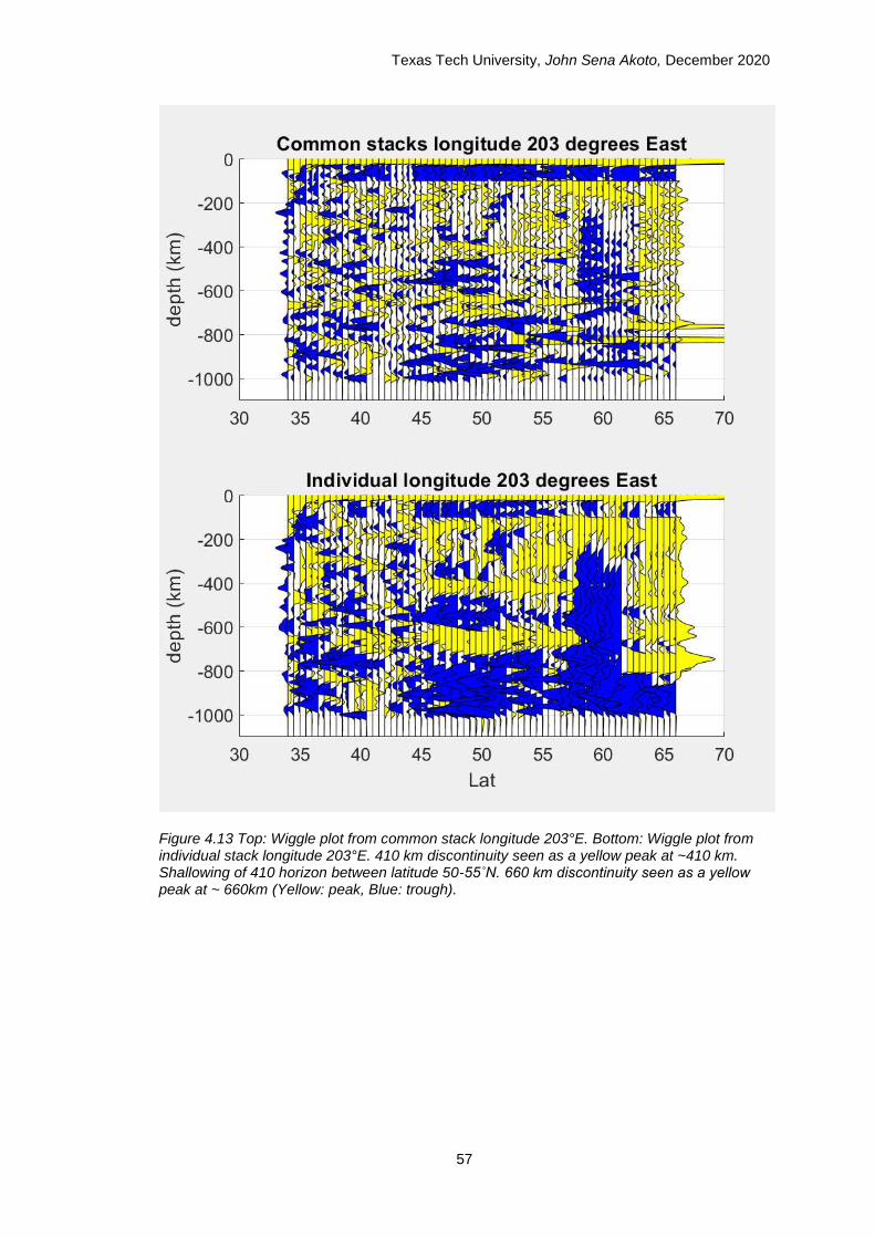
Texas Tech University, John Sena Akoto, December 2020
57
Figure 4.13 Top: Wiggle plot from common stack longitude 203°E. Bottom: Wiggle plot from individual stack longitude 203°E. 410 km discontinuity seen as a yellow peak at ~410 km. Shallowing of 410 horizon between latitude 50-55˚N. 660 km discontinuity seen as a yellow peak at ~ 660km (Yellow: peak, Blue: trough).

Texas Tech University, John Sena Akoto, December 2020
58
Figure 4.14 Colorshading plot for longitude 203°E. 410 km discontinuity seen as a positive amplitude at ~410 km with an uptick in depth between latitude 50-55˚N. 660 km discontinuity seen as a positive amplitude at ~660 km with a decrease in depth between latitude 50-55˚N
4.5 Depth Maps and Velocity Models
In the remainder of our discussion, we will focus on the discontinuities in the TZ because our
most interesting results of tectonic significance are at these depths. The models used in this
section to describe the topography of interesting horizons were made by picking horizons
across all 101 longitudes and 65 latitudes. To better understand the significance of depth
variations observed in the 410 km discontinuity, we will compare our horizon maps to velocity
models generated from the GyPSum 3D Earth Model [Simmons et al., 2010].
Generally, lower than average P and S wave velocity in the mantle corresponds to a hotter
than average mantle temperature, while higher than average P and S wave velocity
corresponds to colder than average mantle temperatures. A hot mantle typically correlates to
the presence of mantle plume or upward convection, while a cold mantle generally associates
with downward convection or a cold subducting slab. And as discussed extensively in the
literature review, the depths of the 410 and 660 are directly affected by local variations in
temperature, where higher than average temperatures deepens the 410 and shallows the
660, while lower than average temperatures shallows the 410 and deepens the 660. Velocity
Am
plit
ud
e

Texas Tech University, John Sena Akoto, December 2020
59
variation observed along these depth horizons are also important to better understand the
depth variations in the TZ boundaries. We expect regions with high velocity to be cold and
areas with low velocity to be warm. If the depth variations correspond well with velocity
variations, we are safe in interpreting the observations as due to temperature variations; if
not, other explanations may be necessary, such as variations in mantle chemistry or
hydration.
4.5.1 410 Discontinuity
The P410P horizon (figure 4.15) has several notable anomalies worth reporting. The P410P
appears to be deeper in the northern regions, relatively shallower in the central parts under
the subduction zone, and then deepens again in the southern portions of the map. Focusing
on specific anomalies, the depth to the 410 km discontinuity beneath the Alaska Subduction
zone (latitude 50°-55° N) is significantly shallower, particularly between longitude 190°-200°E
and 160°-170°E. However, this shallowing trend beneath the subduction zone is disrupted
between longitude 180°E and 190°E, where a deepening of the 410 km discontinuity is
observed. This deep anomaly is relatively local and is confined to 50°-55°N and 180°E and
190°E and trends NW. A second region with deeper than expected depths on the 410
beneath is observed beneath continental Alaska and the region beneath 30°-50°N and 160°-
190°E.
The P wave velocity model for the 410 shows features that correlate strongly with our P410P
model (figure 4.16). Firstly, the model exhibits high P wave velocity in the north and south,
and relatively low P wave velocity in the central regions beneath the subduction zone, which
correlates well with the expected variations in depth that would be anticipated if they are
controlled by temperature variations. More specifically, there is a strong high-velocity anomaly
between 50°-55°N, particularly between 180°-210°E and 160°-170°E, that would be
associated with cold temperatures. The P wave velocity model also shows a relatively high-
velocity anomaly, indicating cold temperatures, between 50°-55°N and 180°-190°E, which
trends NW. This high-velocity (cold) anomaly contradicts the local 410 deepening anomaly
identified in a similar location in our P410P depth map.

Texas Tech University, John Sena Akoto, December 2020
60
Figure 4.15 Topographic map of P410P. 410 km discontinuity shallows in the central portions and deepens in the NE and SW portions of the map.
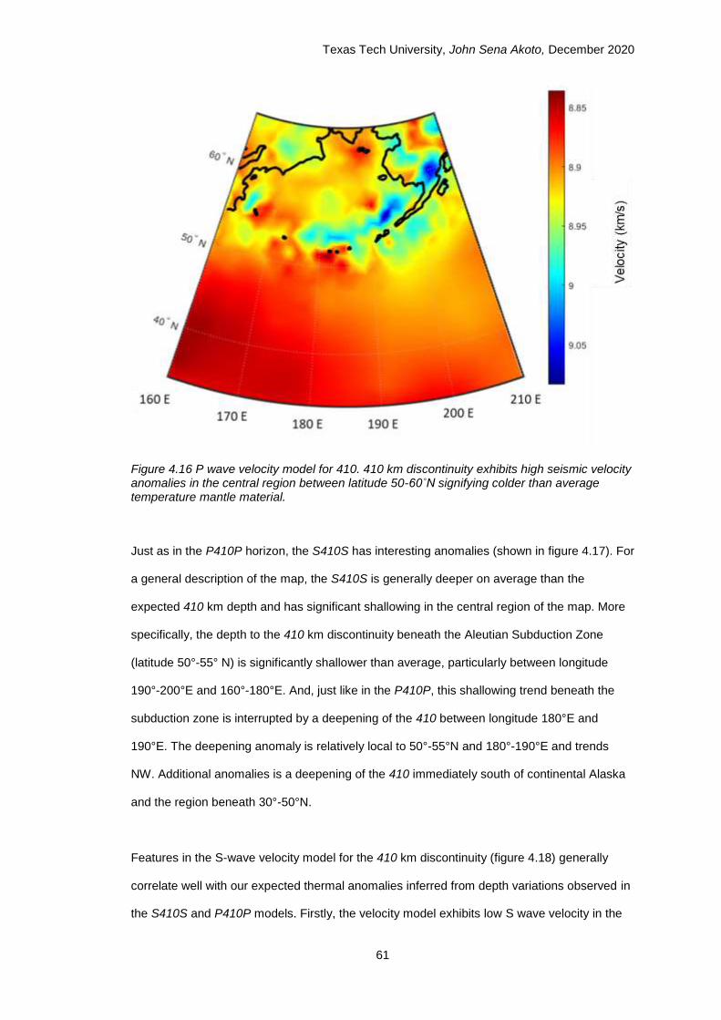
Texas Tech University, John Sena Akoto, December 2020
61
Figure 4.16 P wave velocity model for 410. 410 km discontinuity exhibits high seismic velocity anomalies in the central region between latitude 50-60˚N signifying colder than average temperature mantle material.
Just as in the P410P horizon, the S410S has interesting anomalies (shown in figure 4.17). For
a general description of the map, the S410S is generally deeper on average than the
expected 410 km depth and has significant shallowing in the central region of the map. More
specifically, the depth to the 410 km discontinuity beneath the Aleutian Subduction Zone
(latitude 50°-55° N) is significantly shallower than average, particularly between longitude
190°-200°E and 160°-180°E. And, just like in the P410P, this shallowing trend beneath the
subduction zone is interrupted by a deepening of the 410 between longitude 180°E and
190°E. The deepening anomaly is relatively local to 50°-55°N and 180°-190°E and trends
NW. Additional anomalies is a deepening of the 410 immediately south of continental Alaska
and the region beneath 30°-50°N.
Features in the S-wave velocity model for the 410 km discontinuity (figure 4.18) generally
correlate well with our expected thermal anomalies inferred from depth variations observed in
the S410S and P410P models. Firstly, the velocity model exhibits low S wave velocity in the

Texas Tech University, John Sena Akoto, December 2020
62
north and south, and anomalously high S wave velocity in the central regions beneath the
subduction zone, which matches the observed depth variations in our depth models. More
specifically, there is a strong high-velocity anomaly between 50°-55°N, between 160°-210°E,
which corresponds with the shallowing of the 410 observed in the same location.
However, there are some disparities between our depth model and the velocity model,
specifically, the region in the southwest corner (30°-50°N and 160°-190°E) is clearly a high-
velocity region that would normally be associated with a deeper 410 km, but we observe
shallowing in the 410 in our depth model. Additionally, the deepening of the 410 between 50°-
55°N and 180°-190°E contradicts the high velocity observed in the same location of the
velocity model.
Figure 4.17 Topographic map of S410S. 410 km discontinuity generally shallows in the central portions and deepens in the NE and SW portions of the map.

Texas Tech University, John Sena Akoto, December 2020
63
Figure 4.18 S wave velocity model for 410. 410 km discontinuity exhibits high seismic velocity anomalies in the central region between latitude 50-60˚N signifying colder than average temperature mantle material.
4.5.2 660 Discontinuity
The 660 km discontinuity was only resolved in the SS seismic stacks (figure 4.19 and 4.20).
In the S660S depth model, we observed a general trend of shallowing in the 660 in the
northern and southern regions of the map and a deepening in the central areas, specifically
beneath the Aleutian Subduction Zone. Two zones of deepening anomalies are vividly
observed between latitude 50°-55°N that suggests a downward convecting mantle
(subducting slab). One on the west, between longitude 160°-180°E and the other between
longitude 190°-210°E. In between these two deepening anomalies, from longitude 180°-
190°E, a shallowing anomaly is observed, which implies upward convecting mantle. This
shallowing anomaly has a trend NE direction. Other shallowing anomalies occur directly
beneath continental Alaska, Russia, and the region between latitude 30°-50°N longitude 160°-
210°E.
The S660S depth model (figure 4.19) compares favorably with the S wave velocity model
(figure 4.20) at 660 km. In the velocity model, there are high-velocity zones in the northern

Texas Tech University, John Sena Akoto, December 2020
64
and southern portions of the map, while the central region beneath the subduction zone is of
anomalously low velocity. As explained earlier, lower than average velocity implies a warm
mantle, which in turn implies an upward convecting mantle, which ideally shallows the 660 km
discontinuity. A clear discrepancy between the velocity model and our depth model is the low-
velocity zone beneath continental Russia, which is not reflected in our depth map as a
deepening
Figure 4.19 Topographic map S660S. Deep anomalies are observed between latitude 50-55˚N

Texas Tech University, John Sena Akoto, December 2020
65
Figure 4.20 S wave velocity model for 660. High-velocity anomalies can be seen between latitude 50-60˚N and in the NW corner of the map. High-velocity anomalies suggest colder than average mantle material.
Figure 4.21 P wave velocity model for 660. High-velocity anomalies can be seen between latitude 50-60˚N and in the NW corner of the map. High-velocity anomalies suggest colder than average mantle material.

Texas Tech University, John Sena Akoto, December 2020
66
4.5.3 Transition Zone Isopach
With the S410S and S660S depth maps, an isopach of the transition zone between the
boundaries of the transition zone was produced. The average or expected thickness of the
transition zone is ~ 242 km [Flanagan and Shearer, 1998]. Our thickness model generally
shows an average transition zone thickness in the north and south parts of our study area and
an anomalously thicker transition zone in the central portions of the map. The central portions
beneath the subduction zone –latitude 50-60°N is generally 10-30 km thicker than the
average. This is expected since our S410S, and S660S depth models were respectively
shallower and deeper than average in that region. However, this trend of thicker TZ beneath
the subduction zone is not entirely continuous and breaks off between longitude 180°-190°E,
where the TZ zone is slightly below average thickness.
Figure 4.22 Thickness model for Transition Zone shows thicker than average TZ thickness between latitude 50-55˚N
Texas Tech University, John Sena Akoto, December 2020
67
CHAPTER V
DISCUSSION
5.1 Discussion
From the seismic profiles shown in the results section, shallow discontinuities were observed
around 100 km, 110 km, and 220 km deep (figure 5.1 and 5.2). The P100P phase has a
positive amplitude that occurs when the velocity below the interface is higher than above. The
P110P and P200P phases both have negative amplitudes. Negative phases are the result of
a low-velocity layer beneath a high velocity layer. The LAB is traditionally at 100 km in
oceanic regions but 200 km in continental. Because most of this region is oceanic, it would be
fair to assume the negative P110P phase is the LAB. We believe the region between the 100
and 200 km depths is a lithosphere-asthenosphere transition zone (LATZ) [Ainsworth et al.,
2014]. The mean depth of the LAB in the PP model is 136 km. The LAB shows up in the SS
as a low-velocity zone between ~40-110 km and not as a sharp discontinuity. The mean
depth for the LAB observed in the SS data is 92 km, which compares more favorably with
findings from [Plomerová et al., 2002]. Plomerová et al., 2002 proposed a global model of the
LAB which, suggests a LAB depth of between 70-100 km beneath the Aleutian-Bering sea
region. The depth to the LAB in the PP data was 110 km. The difference in the depths
between the PP and SS data are attributable to 1) the depth in the PP data is relative to the
ocean surface whereas the depth in the SS is relative to the ocean floor, which accounts for
about 5 km of the difference, 2) errors in the reference velocity model used and 3) the
difference in wavelengths between PP and SS data.

Texas Tech University, John Sena Akoto, December 2020
68
Figure 5.1 PP section across longitude 176˚E showing LAB and P220P. The 410 km discontinuity appears at ~410 km and shows a shallowing beneath 50˚N.
Figure 5.2 SS section across longitude 172.5˚E showing LAB. The 660 km discontinuity appears at ~660 km
Generally, higher than average seismic velocities in the mantle corresponds to a hotter than
average mantle temperature, while lower than average seismic velocities correspond to a
Texas Tech University, John Sena Akoto, December 2020
69
colder than average mantle temperature. Variations in velocity can also be related to changes
in the iron content or hydration [Bina and Helffrich, 1994]. A hot mantle typically correlates to
the presence of a mantle plume or hot rising magma while a cold mantle generally associates
with the downwelling of a cold subducting slab [A Cao and Levander, 2010; Q Cao et al.,
2011]. As discussed in the literature review, the depths of the 410 km and 660 km are directly
affected by local variations in temperature where higher than average temperatures deepens
the 410 and shallows the 660. Lower than average temperatures shallows the 410 and
deepens the 660 [G. R. Foulger, 2004]. Since both seismic velocity and depth to the TZ
discontinuities are related to temperature, depth maps to the 410 and 660 should show similar
trends to anomalies observed in maps of the velocity variations for a given depth. We will be
using the velocity models generated from the GyPSum 3D Earth Model for such comparisons
in this work.
The character of the Transition Zone beneath our study area can be understood by
discussing the nature of the 410 and 660, since the response of the Transition zone to the
subducting Pacific Plate provides valuable insight in the dynamics of subduction beneath the
Aleutian Subduction Zone (ASZ). From both our P410P and S410S depth models (figure 5.3
and 5.4), we noticed a 5-20 km shallowing of the 410 beneath the Aleutian Subduction Zone
(ASZ). This shallowing of the 410 suggests the presence of the cold subducting Pacific slab.
In addition, P410P and S410S depth models correlate closely to the 410 P and S velocity
model from the GyPSuM Earth Model[Simmons et al., 2010]. The S660S also shows 10-30
km deepening beneath the Aleutian Subduction Zone (ASZ). This combined shallowing and
deepening of the 410 and 660, respectively, leads to a thickened TZ in the region of
subduction. Our isopach map of the TZ (figure 5.5) demonstrated this expected thickening.
The next region of interest –Region A- is shown in the 410 depth and velocity model (figure
5.3). Region A is a depression in the 410 and a relatively high-velocity anomaly between 50°-
55°N and 180°-170°W, which generally trends NW. Considering that the 410 phase change
has a positive Claperyon slope, deepening at the 410 strongly suggests the presence of
upward convection of hot mantle (low seismic velocity), which contradicts with the high

Texas Tech University, John Sena Akoto, December 2020
70
velocity observed in the velocity model. The apparent contradiction between the depth and
velocity model means anomaly A cannot be uniquely explained by thermal variation,
Claperyon slope, and phase change. Since this anomaly is positioned beneath the Bowers
ridge and only appears in the 410 models, we hypothesize that anomaly A represents
remnants of an ancient slab –possibly from the Kula plate- that sourced the Bowers island
arc. [Verzhbitsky et al., 2007] investigated the tectonics of the northern Pacific Ocean,
concluding that Bowers Ridge formed ~30 Mya, suggests that the Bowers Ridge is a remnant
of an ancient island arc, while others consider it as a Mesozoic island arc [Pitman and
Talwani, 1972], or even as a remnant of an island arc driven to its current location by the Kula
plate[Ben-Avraham and Cooper, 1981].
In regions B, the 410 beneath Alaska is depressed, and correlates with the high-velocity
anomaly observed in the velocity models (figure 5.3). Additionally, the 660 depth model
indicates a deepening underneath Alaska, which is correlated by the high-velocity anomaly
observed in the velocity model (figure 5.4). [Ai et al., 2005] mapped variations in the thickness
of the transition zone beneath south-central Alaska and found general thinning of the
transition zone, by as much as 30 km. Their results compare favorably with the TZ thinning
observed beneath Alaska in our depth models. In general, thinner TZ beneath Alaska imply
the presence of warmer mantle (low seismic velocity) due to exothermic and endothermic
nature of the 410 and 660, respectively.
In regions C and E (figure 5.4), we observe a deepening 660 km discontinuity in our depth
models and a low-velocity anomaly in our velocity model. This anomaly is expected in the
presence of down welling of cool rock (subduction) and infers that the depth anomaly is
related to the subducting Pacific slab. Considering Claperyon slope, the 660 beneath these
anomalies deepens as expected. However, the location of the anomaly in region C is
extended south of the ASZ, which suggests an irregular path of subduction. It is known that in
this part of the subduction zone, there is more strike-slip motion on the slab than reverse fault
and is characterized by an increasing subduction angle and slab rollback [Zhu and Xu, 2019].
We propose that since the Pacific Plate subducts at a high angle, it may rollback or rollover

Texas Tech University, John Sena Akoto, December 2020
71
on itself. Because of this unique motion, we believe the plastic subducting plate puddles on
top of the 660 beneath the ASZ and flows to lower latitudes. The S wave velocity map at the
660 km depth has a high-velocity anomaly in regions C and E, which further supports the idea
of cold slab material pooling atop the 660 below ASZ.
The depth anomalies in regions C and E show approximately a 30 km of deepening of the
660, which cannot be accounted for solely based on the thermal anomaly. Studies show that
the presence of water stored within an oceanic slab can depress the 660 by up to 15 km [A
Cao and Levander, 2010]. Moreover, using a Claperyon slope of -1.3 MPa/K [K Litasov et al.,
2005; K D Litasov, 2005], a 30 km depression in the mantle requires the Pacific plate to be
~850°K cooler than the surrounding mantle. This is unlikely since the typical average
temperature difference between a cold slab and mantle temperature at 660 km is ~670°K
(Slab temperature ~1180°K and mantle temperature ~1850°K) [A Cao and Levander, 2010].
Thus, suggesting that the ~30 km depressions observed beneath region C and E are likely
dependent on thermal anomalies and presence of water. The Transition Zone has been
shown to be a water reservoir where water –in the form of dense hydrous magnesium-silicate
phases (DHMS)- is filtered out from wet subduction slabs through a slab dehydration process
[Richard et al., 2006]. We speculate that the slab material atop the 660 is dehydrating and the
release of water contributes to the deepening of the 660 km discontinuity observed in regions
C and E.
From the isopach of the depth difference between the 660 and 410 (figure 5.5), we observe
that the transition zone is thicker than average beneath the subduction zone. This strongly
infers the presence of the subducting Pacific Plate and confirms the anti-correlated Claperyon
slopes of the 410 and 660. Nevertheless, the majority regional extent of this anomaly is
caused by deepening of the 660, since we would not expect pooling on the 410.

Texas Tech University, John Sena Akoto, December 2020
72
Figure 5.3 (I) Topographic map of 410. (II) Velocity model of 410. ASZ (white dashed line) represents Aleutian subduction zone; A is a deepening anomaly that demarcates 410 beneath Bowers Ridge; B is a deepening anomaly that demarcates 410 beneath Alaska
Figure 5.4 (I) Topographic map of 660. (II) Velocity model of 660. ASZ (white dashed line) represents Aleutian subduction zone; C and E are deepening anomalies that demarcates pooling of high-velocity slab material, colder than average slab material at 660; D demarcates 660 beneath Alaska
I II
I II

Texas Tech University, John Sena Akoto, December 2020
73
Figure 5.5 Thickness of transition zone. C and E show areas with thicker than average TZ where the subducting slab might be puddling and depressing the 660 significantly
5.1.1 Puddle Zones: Anomalies C and E in the Transition Zone
To further analyze anomalies C and E observed on the 660 depth and velocity models; cross-
sections were made along AA’ (170°E), BB’ (185°E), DD’ (200°E), FF’ (42°N), and GG’ (50°N)
(figure 5.7 to 5.17). Profiles AA’, DD’, and GG’ were selected because they transect
anomalous zones of significance while BB’ and FF’ cross relatively average zones and thus
serve as control profiles. Profile DD’ and AA’ show the dip view across anomalous zones E
and C, respectively, while latitude GG’ illustrates the strike view along the subduction zone

Texas Tech University, John Sena Akoto, December 2020
74
and the anomalous zones (C, E). Profile lines are shown in figure 5.6 below
Figure 5.6 Depth map to 660 showing anomaly C and E, and profile lines AA’ (170°E), BB’ (185°E), DD’ (200°E), FF’ (42°N), and GG’ (50°N)
In AA’, the 410 and 660 is generally flat up to 55°N after which the 410 becomes less visible,
and the 660 deepens significantly. The 520 discontinuity becomes visible after 55°N, which
suggests a change in mantle temperature. In general, the 520 is seismically less visible than
the 410 and 660 because of its low-velocity contrast and gradational Clapyeron slope, and
occurs over a wider range of 30-50 km thick [Bostock, 1996]. We suggest that the observance
of the 520 in figure 5.7 and 5.8 is a result of mantle chilling caused by the subducting slab.
We propose that the low temperature of the slab chills the mantle within the TZ, which
steepens the temperature and velocity gradient across the 520, thereby reducing the depth
range for the phase change, making the S520S phase stronger and more visible. Profile BB’
exhibits similar features as that seen in AA’. A ~30 km deepening of the 660 beneath anomaly
E, and a visible 520.
H’
H

Texas Tech University, John Sena Akoto, December 2020
75
Figure 5.7 Profile AA’ showing 520 km discontinuity and 660 km discontinuity deepening beyond latitude 50°N (anomaly E)
Figure 5.8 Profile DD’ showing 660 deepening beneath latitude 45-50°N (anomaly E). 520 km discontinuity visible after latitude 55˚N.
Where visible in profile GG’, the 410 is elevated ~10 km, as is expected in the response of the
olivine to wadsleyite phase change[G. R. Foulger, 2004]. The 660 is generally conspicuous
the entire profile except for between 180-195° N. The deepening of the 660 to ~700 km is
observed beneath zones C and E, as shown in figure 5.9. Again, it is apparent that there are
pieces of Pacific slab material causing a deepening of the 660 beneath zones C and E.
In the control profile FF’, that does not cross C and E, the 410 and 660 are visible and
consistently flat. This gives us the confidence to infer that the respective shallowing and

Texas Tech University, John Sena Akoto, December 2020
76
deepening of the 410 and 660 observed in GG’ and not in FF’ is caused by the subducting
Pacific Plate.
Figure 5.9 Profile GG’ showing section across anomaly C and E. 660 deepened to ~700 km.
Figure 5.10 Control profile FF’, the 660 is observed at the expected depth of ~660 km.
Next, we look to the velocity profiles from GyPSuM to see if they exhibit the same trends
observed in our depth models. Profile AA’ shows the 660 deepens to ~690 km across
anomaly C, while the 660 in the control profile BB’, which does not cross the depth anomaly,
has a maximum depth of the 670 km. Aside from the lower than average temperature of the
subducting slab depressing the 660 [G. R. Foulger, 2004], slab dehydration within the

Texas Tech University, John Sena Akoto, December 2020
77
Transition Zone has also been shown to depress the 660 by up to15km [A Cao and Levander,
2010; Mohamed et al., 2014]. This observation suggests that the depth anomaly C can be
linked to cold subducting slab material atop the 660.
Figure 5.11 (A) Variation of 660 observed in profile AA’. (B)Enlargement of the dashed box around the 660 in profile AA’. The 660 is deepened by up to ~30km.
Figure 5.12 (A) Variation of 660 observed in profile BB’. (B) Enlargement of the dashed box around the 660 in profile BB’. 660 here is relatively flat with a maximum deepening of 10 km.
In the velocity profile at DD’ that crosses anomaly E, the 410 appears relatively flat, and the
660 is noticeably depressed to ~690 (figure 5.13c). A velocity reversal (feature II from figure

Texas Tech University, John Sena Akoto, December 2020
78
5.13b), which indicates an abrupt change in velocity trend, is partly discernable between 57°
and 63° N. We suggest that the sudden increase and subsequent decrease of velocity across
the reversal is indicative of partial melting of the Pacific slab atop the 660 km. A high-velocity
anomaly appears between 62.5-66°N seen at 520 km (feature I from figure 5.13b). The
anomalously high velocity supports the “mantle chilling effect” explained earlier where the
subducting slab cools the nearby mantle, causing a relatively sharper velocity contrast at the
520.
Figure 5.13 (A) Absolute velocity profile for longitude DD’. (B) Enlargement of the dashed box showing 410, 520, and 660. Deepening of the 660 is observed along with a velocity reversal (II) of the 660. The 520 (I) visible after latitude 60°N. (C) Enlargement of the dashed box around the 660 to show ~30 deepening on the 660 km discontinuity
GG’ (figure 5.14) shows us a strike view of velocities beneath the subduction zone that
intersects C and E. As expected, high-velocity anomalies are observed between 165°-175° N
and 195°-200° N, which coincides with depth anomalies at C and E. Moreover, the 660 is
depressed by ~20 km and ~30 km at C and E respectively.

Texas Tech University, John Sena Akoto, December 2020
79
Figure 5.14 (A) Absolute velocity profile for latitude GG’. (B) Enlargement of the dashed box showing high velocity on top of the 660 beneath anomaly C and E.
Studies of velocity perturbations are usually superior to absolute velocities because they may
more closely reflect temperature and (or) compositional anomalies [A Cao and Levander,
2010]. In the relative velocity profile AA’ (figure 5.15), we notice a low-velocity anomaly
between 0-200 km, which suggests hot temperature, between 55˚-66˚N. This high-temperature
anomaly is north of the subduction zone and is relatively shallow. We suggest that this
anomaly can be attributed to partial melting occurring in the shallow lithosphere as the Pacific
Plate subducts [Marsh and Carmichael, 1974]. The region below the 520 is anomalously cold,
possibly because of cooling from the subducting slab sitting at the base of the TZ. Beneath
this, we notice two sub-vertical high-velocity anomalies (with colder than average temperature)
between latitude 50°N-60°N at depths between 300-660 km, which appear to puddle after 660.
In figure 5.15 and 5.16, we show the velocity perturbation profile along AA’ and DD’,
respectively. Profile DD’ exhibits similar features as we discussed for profile AA’; firstly, there is
a shallow low-velocity anomaly beyond latitude 50°N that we attribute to partial melts sourced
from the subducting slab. The 520 is distinctly visible and it is probably due to mantle cooling
from the subducting slab. In profile DD’, we notice two sub-vertical high-velocity anomalies
(cold slab) between 50°-60°N that terminate at ~660 km. Finally, in the velocity perturbation
profile GG’, we observe that the TZ beneath the Aleutian Subduction Zone is of higher than
average velocity inferring colder than average temperatures. These observations imply the
presence of cold subducting material in the TZ beneath the subduction zone.

Texas Tech University, John Sena Akoto, December 2020
80
Figure 5.15 S-Wave velocity perturbation profile AA’. High-velocity anomalies are observed between latitude 50-55°N (anomaly C). The deepening of the 660 is noticed between latitude 50-65°N.
Figure 5.16 S-Wave velocity perturbation profile DD’. High-velocity anomalies are observed between latitude 50-60°N (anomaly C). The deepening of the 660 is noticed between latitude 50-60°N. The 520 km discontinuity is visible beyond latitude 60°N.

Texas Tech University, John Sena Akoto, December 2020
81
Figure 5.17 S-Wave velocity perturbation profile GG’. The TZ in profile GG’ (across anomaly C and E) is generally of high velocity suggesting a cold TZ
Texas Tech University, John Sena Akoto, December 2020
82
CHAPTER VI
CONCLUSIONS
6.1 Geological Implications
An analysis of the distribution of seismic attributes around the Alaska Subduction region was
conducted, and from our results and discussion, we suggest the following conclusions:
1. The 410 (olivine to wadsleyite phase change) shallows by up to 20 km, the 660
(ringwoodite to perovskite and ferropericlase phase change) deepens by up to 30 km.
This results in a thicker than average Transition Zone and suggests a cooler than
average Transition Zone beneath the Aleutian subduction zone.
2. Our geophysical models of the study area show that the 410 deepens underneath
Bowers Ridge, which suggests upward convection of hot mantle (low seismic
velocity). However, the velocity model is at odds with the depth model, instead high
velocities infer a cold mantle (high seismic velocity) beneath the Bowers ridge. We
hypothesize that this anomaly represents remnants of an ancient slab –possibly from
the Kula plate- that sourced the Bowers island arc.
3. Based on the depth model, velocity models, and the thicker than usual TZ from SdS
depth estimates, we suggest that the subducting Pacific slab pools atop of the 660,
causing it to deepen due to the presence of the plastic cold slab. However, the depth
anomaly on the 660 cannot be explained by temperature anomaly alone, and we
believe it is further depressed because of dehydration of the slab.
4. Beyond latitude 60°N, the 520 was regularly observed in our seismic profiles. We
suggest that the visibility of the 520 in close vicinity to the subducting slab is because
of the “mantle chilling effect” at the base of the TZ. We believe the “mantle chilling
effect” caused by the hypothesized slab puddling on the 660 increases the velocity
contrast in that region resulting in a sharp 520 discontinuity.

Texas Tech University, John Sena Akoto, December 2020
83
Figure 6.1 Cartoon model of Pacific plate subduction beneath the Aleutian subduction zone across profile HH’. Shows elevated 410, 520, and deepened 660. Convective current and mantle chilling leads to sharp 520. Slab dehydration contributes to ~30km deepening observed on the 660, and possible slab rollback on the 660 accounts for cold anomaly seen beneath the ASZ at lower latitude.
Texas Tech University, John Sena Akoto, December 2020
84
REFERENCES
Ai, Y., D. Zhao, X. Gao, and W. Xu (2005), The crust and upper mantle discontinuity structure beneath Alaska inferred from receiver functions, Physics of the Earth and Planetary Interiors, 150(4), 339-350, doi:10.1016/j.pepi.2004.12.002.
Ainiwaer, A. (2014), Synthetic study in amplitude and frequency content of the P410P phases from common upper mantle discontinuity, Texas Tech University.
Ainiwaer, A., and H. Gurrola (2018), Wavefield iterative deconvolution to remove multiples and produce phase specific Ps receiver functions, Geophysical Journal International, 212(3), 2016-2030, doi:10.1093/gji/ggx454.
Ainsworth, R., J. Pulliam, H. Gurrola, and D. Evanzia (2014), Sp receiver function imaging of a passive margin: Transect across Texas's Gulf Coastal Plain, Earth and Planetary Science Letters, 402, 138-147, doi:10.1016/j.epsl.2014.05.056.
Anderson, D. L. (2007), New Theory of the Earth, doi:10.1017/cbo9781139167291.
Ben-Avraham, Z. V. I., and A. K. Cooper (1981), Early evolution of the Bering Sea by collision of oceanic rises and North Pacific subduction zones, Geological Society of America Bulletin, 92(7), doi:10.1130/0016-7606(1981)92<485:Eeotbs>2.0.Co;2.
Bercovici, D., and S. Karato (2003), Whole-mantle convection and the transition-zone water filter, Nature, 425(6953), 39-44, doi:10.1038/nature01918.
Bina, C. R. (2017), Mantle Discontinuities, Reviews of Geophysics, 29(S2), 783-793, doi:10.1002/rog.1991.29.s2.783.
Bina, C. R., and G. Helffrich (1994), Phase transition Clapeyron slopes and transition zone seismic discontinuity topography, Journal of Geophysical Research, 99(B8), doi:10.1029/94jb00462.
Birch, F. (1952), Elasticity and constitution of the Earth's interior, Journal of Geophysical Research, 57(2), 227-286, doi:10.1029/JZ057i002p00227.
Bostock, M. G. (1996), Psconversions from the upper mantle transition zone beneath the Canadian landmass, Journal of Geophysical Research: Solid Earth, 101(B4), 8393-8402, doi:10.1029/95jb03741.
Brown, J. R., S. G. Prejean, G. C. Beroza, J. S. Gomberg, and P. J. Haeussler (2013), Deep low-frequency earthquakes in tectonic tremor along the Alaska-Aleutian subduction zone, Journal of Geophysical Research: Solid Earth, 118(3), 1079-1090, doi:10.1029/2012jb009459.
Bullen, K. E. (1986), An Introduction to the Theory of Seismology, Cambridge University Press, Cambridge, United Kingdom.
Cao, A., and A. Levander (2010), High-resolution transition zone structures of the Gorda Slab beneath the western United States: Implication for deep water subduction, Journal of Geophysical Research, 115(B7), doi:10.1029/2009jb006876.
Cao, Q., R. D. van der Hilst, M. V. de Hoop, and S. H. Shim (2011), Seismic Imaging of Transition Zone Discontinuities Suggests Hot Mantle West of Hawaii, Science, 332(6033), 1068-1071, doi:10.1126/science.1202731.

Texas Tech University, John Sena Akoto, December 2020
85
Chambers, K., J. H. Woodhouse, and A. Deuss (2005), Topography of the 410-km discontinuity from PP and SS precursors, Earth and Planetary Science Letters, 235(3-4), 610-622, doi:10.1016/j.epsl.2005.05.014.
Collier, J. D., and G. R. Helffrich (1997), Topography of the ''410'' and ''660'' km seismic discontinuities in the Izu-Bonin subduction zone, Geophysical Research Letters, 24(12), 1535-1538, doi:Doi 10.1029/97gl01383.
Cordery, M. J., G. F. Davies, and I. H. Campbell (1997), Genesis of flood basalts from eclogite-bearing mantle plumes, Journal of Geophysical Research: Solid Earth, 102(B9), 20179-20197, doi:10.1029/97jb00648.
D. W. Scholl, E. C. B., M. S. Marlow (1975), Plate Tectonics and the Structural Evolution of the Aleutian-Bering Sea Region, Geological Society of America, doi:10.1130/SPE151-p1.
Deuss, A. (2009), Global Observations of Mantle Discontinuities Using SS and PP Precursors, Surveys in Geophysics, 30(4-5), 301-326, doi:10.1007/s10712-009-9078-y.
Duncan, G. M. (2012), Processing innovations to improve PP precursor analysis and increase frequency content of studies in the Mid-Pacific, 125 pp, Texas Tech University.
Fischer, K. M., H. A. Ford, D. L. Abt, and C. A. Rychert (2010), The Lithosphere-Asthenosphere Boundary, Annual Review of Earth and Planetary Sciences, 38(1), 551-575, doi:10.1146/annurev-earth-040809-152438.
Flanagan, M. P., and P. M. Shearer (1998), Global mapping of topography on transition zone velocity discontinuities by stackingSSprecursors, Journal of Geophysical Research: Solid Earth, 103(B2), 2673-2692, doi:10.1029/97jb03212.
G. R. Foulger, B. R. J. (2004), Variations in Global Transition Zone Thickness.
Gutenberg, B. (1959), Physics of the Earth's Interior, Academic Press.
Helffrich, G. (2000), Topography of the transition zone seismic discontinuities, Reviews of Geophysics, 38(1), 141-158, doi:Doi 10.1029/1999rg000060.
Hilde, T. W. C., S. Uyeda, and L. Kroenke (1977), Evolution of the western pacific and its margin, Tectonophysics, 38(1-2), 145-165, doi:10.1016/0040-1951(77)90205-0.
Ishii, T., et al. (2018), Complete agreement of the post-spinel transition with the 660-km seismic discontinuity, Sci Rep, 8(1), 6358, doi:10.1038/s41598-018-24832-y.
Karig, D. E. (1972), Remnant Arcs, Geological Society of America Bulletin, 83(4), doi:10.1130/0016-7606(1972)83[1057:Ra]2.0.Co;2.
Kennett, B. L. N., and E. R. Engdahl (1991), Traveltimes for global earthquake location and phase identification, Geophysical Journal International, 105(2), 429-465, doi:10.1111/j.1365-246X.1991.tb06724.x.

Texas Tech University, John Sena Akoto, December 2020
86
Kennett, B. L. N., E. R. Engdahl, and R. Buland (1995), Constraints on seismic velocities in the Earth from traveltimes, Geophysical Journal International, 122(1), 108-124, doi:10.1111/j.1365-246X.1995.tb03540.x.
Kienle, J. (1971), Gravity and magnetic measurements over Bowers Ridge and Shirshov Ridge, Bering Sea, Journal of Geophysical Research, 76(29), 7138-7153, doi:10.1029/JB076i029p07138.
Kumar, P., and H. Kawakatsu (2011), Imaging the seismic lithosphere-asthenosphere boundary of the oceanic plate, Geochemistry, Geophysics, Geosystems, 12(1), n/a-n/a, doi:10.1029/2010gc003358.
Lawrence, J. F., and P. M. Shearer (2006), A global study of transition zone thickness using receiver functions, Journal of Geophysical Research: Solid Earth, 111(B6), n/a-n/a, doi:10.1029/2005jb003973.
Litasov, K., E. Ohtani, A. Sano, A. Suzuki, and K. Funakoshi (2005), In situ X-ray diffraction study of post-spinel transformation in a peridotite mantle: Implication for the 660-km discontinuity, Earth and Planetary Science Letters, 238(3-4), 311-328, doi:10.1016/j.epsl.2005.08.001.
Litasov, K. D. (2005), Wet subduction versus cold subduction, Geophysical Research Letters, 32(13), doi:10.1029/2005gl022921.
Ludwig, W. J. (1971), Sediment distribution in the Bering Sea; Bowers Ridge, Shirshov Ridge and enclosed basins, Journal of Geophysical Research, 76, 6367.
Marsh, B. D., and I. S. E. Carmichael (1974), Benioff zone magmatism, Journal of Geophysical Research, 79(8), 1196-1206, doi:10.1029/JB079i008p01196.
Mohamed, A. A., S. S. Gao, A. A. Elsheikh, K. H. Liu, Y. Yu, and R. E. Fat-Helbary (2014), Seismic imaging of mantle transition zone discontinuities beneath the northern Red Sea and adjacent areas, Geophysical Journal International, 199(2), 648-657, doi:10.1093/gji/ggu284.
Nur, A., and Z. Ben-Avraham (1978), Speculations on Mountain Building and the Lost Pacifica Continent, Journal of Physics of the Earth, 26(Supplement), S21-S37, doi:10.4294/jpe1952.26.Supplement_S21.
Pitman, W. C., and M. Talwani (1972), Sea-Floor Spreading in the North Atlantic, Geological Society of America Bulletin, 83(3), doi:10.1130/0016-7606(1972)83[619:Ssitna]2.0.Co;2.
Plomerová, J., D. Kouba, and V. Babuška (2002), Mapping the lithosphere–asthenosphere boundary through changes in surface-wave anisotropy, Tectonophysics, 358(1-4), 175-185, doi:10.1016/s0040-1951(02)00423-7.
Richard, G., D. Bercovici, and S.-I. Karato (2006), Slab dehydration in the Earth's mantle transition zone, Earth and Planetary Science Letters, 251(1-2), 156-167, doi:10.1016/j.epsl.2006.09.006.
Ritsema, J., L. A. Rivera, D. Komatitsch, J. Tromp, and H.-J. van Heijst (2002), Effects of crust and mantle heterogeneity on PP/P and SS/S amplitude ratios, Geophysical Research Letters, 29(10), 72-71-72-74, doi:10.1029/2001gl013831.

Texas Tech University, John Sena Akoto, December 2020
87
Rogers, K. (2013), Investigation of the upper mantle beneath the Hawaiian Island chainusing PP-precursors, Texas Tech University.
Schäfer, J., I. Wölbern, and G. Rümpker (2009), Depth variations of the 410 and 520 km-discontinuities beneath Asia and the Pacific from PP precursors, Geophysical Research Letters, 36(12), doi:10.1029/2009gl038374.
Scholl, D. W., E. C. Buffington, and D. M. Hopkins (1968), Geologic history of the continental margin of North America in the Bering Sea, Marine Geology, 6(4), 297-330, doi:10.1016/0025-3227(68)90021-2.
Simmons, N. A., A. M. Forte, L. Boschi, and S. P. Grand (2010), GyPSuM: A joint tomographic model of mantle density and seismic wave speeds, Journal of Geophysical Research, 115(B12), doi:10.1029/2010jb007631.
Steven Holbrook, W., D. Lizarralde, S. McGeary, N. Bangs, and J. Diebold (1999), Structure and composition of the Aleutian island arc and implications for continental crustal growth, Geology, 27(1), doi:10.1130/0091-7613(1999)027<0031:Sacota>2.3.Co;2.
Verzhbitsky, E. V., M. V. Kononov, and V. D. Kotelkin (2007), Plate tectonics of the northern part of the Pacific Ocean, Oceanology, 47(5), 705-717, doi:10.1134/s000143700705013x.
Zhu, R., and Y. Xu (2019), The subduction of the west Pacific plate and the destruction of the North China Craton, Science China Earth Sciences, 62(9), 1340-1350, doi:10.1007/s11430-018-9356-y.

Texas Tech University, John Sena Akoto, December 2020
88
APPENDICES
Appendix A – Processing Workflow and Codes
SAC to MAT Conversion
IRIS DMC saves time series PdP and SdS data in a sac format. SACtoMATB_2015 converts
data from sac to mat, which is compatible in Matlab. Below is SACtoMATB_2015 and its
subroutine SACTOOLB_2015.
function SACtoMATB_2015(outP) %This program will convert your SAC files into 3 component mat files
and %put them in a new directory called dirsort.
%ex: dirsortcl_2011 nowdir=pwd; islash=find(nowdir=='\'); outdir3=[outP ':\MAT' nowdir(islash(2):end)] outdir1=[outP ':\MAT1' nowdir(islash(2):end)] mkdir(outdir3) mkdir(outdir1)
A=dir('*BHZ*.SAC'); %searches current directory for all BHZ files,
sets up structural array which holds info for each file O=length(A); %number of BHZ files found z=0; oldname='ZZZZZZZZZZZZZ'; for i=1:O; %runs loop for all BHZ files
fnameZ=A(i).name %searches the structural array 'A' for the file
name if fnameZ(1:13)==oldname disp('already did a station by that name') else whereBHZ=findstr(fnameZ,'BHZ'); fname=dir([fnameZ(1:(whereBHZ-1)) '*'
fnameZ((whereBHZ+3):end-10) '*']);
if length(fname) ==3 SACTOOLB_2015(fname,outdir3); %runs SACTOOL2010C program end if length(fname) ~=3 fname(1).name=fnameZ; SACTOOLB_2015(fname,outdir1); %runs SACTOOL2010C program end end oldname=fnameZ(1:13); end
function SACTOOL_2015(filename,out_path) %MatTimes Tool:

Texas Tech University, John Sena Akoto, December 2020
89
% %SACTOOL Imports Seismic Analysis Code files (SAC). % 1) SACTOOL(FILENAME,DIRECTORY) Imports a single file from the SAC % format to a Matlab data file (.mat) as a structured array
(variable % with fields). The output name is the same as the string argument % FILENAME and the file is saved in the current directory.
DIRECTORY % is a string argument naming the directory (i.e.,
'C:/MatTimes/Data/'). % If DIRECTORY is left off, it is assumed that the current
directory % contains the file. % % 2) SACTOOL(LIST,DIRECTORY) Imports multiple files contained within
the list. % To generate LIST, simply use the Matlab DIR command like the % following: % % LIST=dir(FILES) % % where FILES is a string argument that uses the wildcard (*) to % make a list. LIST will be a structured array consisting of one % column. % % 3) SACTOOL(LIST3,DIRECTORY,NAMES) % LIST3 is similar to LIST except that it is designed to load in
three % seismic components to save to a single file as a multi-
dimensional % structured array. NAMES is a structured list of file names for
each % row in LIST3. A row of files in LIST3 will be combined into a
single % file in the corresponding row or column in NAMES. The three
components % will saved within NAMES as data(1:3) where "data" is a structured
array. % See example below. % % IMPORTANT NOTES: % % To choose a particular SAC format (user-defined header fields),
four % inputs are necessary: SACTOOL(FILE,DIRECTORY,OUTNAME,FLAG). % % For TTU format: FLAG = 1 % User5, User6, User7 and User8 must have actual event time
information % so that MatTimes can determine travel time markers for the
imported % data stream. User5 = Julian Day, User6 = event hour, User7 =
event minute, % User8 = event seconds. All of these fields will be combined
during % importation to a field named "evtime". The actual data stream
beginning % time will be in the field named "begintime". "Streamtime" will
contain % the data stream length in seconds. %

Texas Tech University, John Sena Akoto, December 2020
90
% For RISTRA format: FLAG = 2 % Most likely format to use. % % % EXAMPLES for PC: % % %Load in a z-component data file % load dir_path %(file generated with SETUP with path names for
example only) % FILENAME=[whereami '/Data/event0920z']; %(whereami from
dir_path) % SACTOOL2007(FILENAME) %create Matlab file % % %Load in all three components for the same event, 0920. % load dir_path %(this does not have to be used in real
situations) % DIRECTORY=[whereami '/Data/']; % LIST=dir([DIRECTORY 'event0920*']); % SACTOOL2007(LIST,DIRECTORY) % % %Load in three components for a multi component file creation % %Try this in the "Data" directory (delete all example ".mat"
files first) % LIST3=[dir('ev*e') dir('ev*n') dir('ev*z')]; % DIRECTORY=[]; % NAMES.name='event0920'; % SACTOOL2007(LIST3,DIRECTORY,NAMES); % %look at some input % load(NAMES(1).name) % data(2) % plot3comp(NAMES(1).name) % % %if LIST3 is long, it is not convenient to type in all output
names, in such % %a case you could do a form of the following for your file
name structures: % % LIST3=[dir('ev*e') dir('ev*n') dir('ev*z')]; %make data file
list % [a,b]=size(LIST3); % for i=1:a % lname=length(LIST3(i).name); % NAMES(i).name=LIST3(i).name(1:lname-1) %use same name
minus last character % %as a
file name % end % % %disp(['SACTOOL...Working']); %directory is ./ if nargin=1
jout=0 [b]=length(filename)
%loop through components for j=1:b; %determine string file name name=[filename(j).name] fname=[name]; [abort,h1,h2,h3,data2]=READSAC_2015(name); %read file\

Texas Tech University, John Sena Akoto, December 2020
91
if abort==666, break, end tsec=h2(6)./(1000); sec=h2(5)+tsec; nztime=[h2(1:5)]; nztime(5)=sec; nzdeltatime=h1(8); nzdeltamin=ceil(nzdeltatime/60); nzdeltasec=nzdeltatime-60*nzdeltamin; evtime=nztime+[0 0 0 nzdeltamin nzdeltasec]; if evtime(5) < 0, evtime(4)=evtime(4)-1; evtime(5)=evtime(5)+60;
end if evtime(4) < 0, evtime(3)=evtime(3)-1; evtime(4)=evtime(4)+60;
end if evtime(3) < 0, evtime(2)=evtime(2)-1; evtime(3)=evtime(3)+24;
end if evtime(2) < 0, evtime(1)=evtime(1)-1; evtime(2)=evtime(2)+365;
end % evtime=[h(1:5)] %begintime=[h(1) h(24:26) round(h(27)*100000)/100000];
filetime=jconvnamehg(name); begintime=nztime; streamtime=round(h1(7)*100000)/100000;
fields=['name','import','evtime','begintime','nztime','filetime','str
eamtime','station_lat','station_lon',...
'station_elevation','borehole_depth','compass_az','compass_inc','even
t_lat','event_lon','event_depth','magnitude',...
'arc_distance','azimuth','backazimuth','gcarc','deltatime','SACT0','S
ACT1',... 'SACT2','SACT3','SACT4','SACT5','SACT6','dt','data']; % h=[h2(1:6) round(h1(1)*1000000)/1000000 h1(6=h8:7)
h1(11=h10:17) h1(32=h17:37=h22) h1(39) h1(46=h24:54) h1(58=h33:59)];
fill=[fname,datestr(datenum(now)),evtime,begintime,nztime,filetime,st
reamtime,h1(32),h1(33),...
h1(34)/1000,h1(35),h1(58),h1(59),h1(36),h1(37),h1(39),h1(50),... h1(51),h1(53),h1(52),h1(54),nzdeltatime,h1(12),h1(13),...
h1(14),h1(15),h1(16),h1(17),h1(18),(floor(h1(1)*1000000)/1000000),[da
ta2(:)']];
d=cell2struct(fill,fields,2); data(j)=d; %if j == 1, hold off, plot(data2,'r'), end %if j == 2, hold on, plot(data2,'b'), end %if j == 3, hold on, plot(data2,'g'), end
end if abort==666, evtime(1)=-10, end if evtime(1) > 0; failflag=0; Devent=[data(1).event_lat data(1).event_lon]; Dsta=[data(1).station_lat data(1).station_lon]; fnameoutb=[out_path '\' [fname(1:end-3) '.mat']]; save(fnameoutb,'data');

Texas Tech University, John Sena Akoto, December 2020
92
fclose('all'); %avoid "too many files open" problem else failflag=1; fname=[fname ' failed to read']; end
%pause
%close(wb) %disp(['SACTOOL...Done'])

Texas Tech University, John Sena Akoto, December 2020
93
Cutting
ALLCUT_2015 cuts both PdP and SdS data. It calls on the sub-routine CUTDATA_2015 to
perform cuts. Below is the code for ALLCUT_2015 and CUTDATA_2015.
function ALLCUT_2015(phase,cutdata_window,istart,ftype)
% ALLCUT_2015(phase,cutdata_window,istart,ftype,network) % ALLCUT_2015('P',[30 150],1,'BH','*') % ALLCUT_2015('SdS',[350 120],1,'BH','*') % % warning off all %will disable warnings that tell us the directory we
are trying to create already exists
dirs=dir('*') home=pwd for i=istart:(length(dirs)-1) i=i; if exist(dirs(i).name) == 7 dir1=dirs(i).name; if dir1(1)=='.' disp(['did not process ' dir1]) else cd(dir1); %save(MASTER_PATH,'events') % disp(['Events left is ' events_left '.']) events=dir(['*' ftype '*.mat']); outd=pwd; imat=findstr(outd,'MAT'); outd=['G:\CUT_' phase outd(imat+3:end)]
CUTDATA_2015(events,phase,[],'iasp91',cutdata_window,outd); %runs
program cd(home) i=i; dir1=dirs(i).name; save(['start_all_' phase],'i') end end end
end
function CUTDATA_2015(file,phase,variable,model,window,outd) %MatTimes Tool: % %CUTDATA Cuts data about an input phase based on a time window. % 1) CUTDATA(LIST,PHASE,VARIABLE,MODEL,WINDOW,MODE) % Cuts down data within the LIST about PHASE according to % WINDOW. LIST is a structured list naming each file to % be snipped. See SACTOOL option 2 for LIST creation. PHASE % is a string argument naming the phase to center about (i.e., % 'P'). If the phase has a depth variable, such as Pds, the % input VARIABLE must be given as a value. Otherwise, VARIABLE % should be an empty cell ([]). MODEL is the velocity model % to use when determining the phase marker. WINDOW is the

Texas Tech University, John Sena Akoto, December 2020
94
% window about the phase marker to keep. WINDOW(1) is the % pre-phase time window to keep in seconds. WINDOW(2) is the % post-phase time to keep in seconds. MODE determines whether % or not the Matlab data file is deleted. % % % NOTE: The header information will be adjusted to the cut. Also, % if the data file has three components, all will be cut and % all headers will be adjusted accordingly. If the given phase % has multiple times, the cut will be about the minimum and % maximum times expanding the total stream time. % % ex: CUTDATA_2014(dir('*.mat'),'P',[],'iasp91',[30
150],'c:\P_MAT\neme..')
goback=pwd; %stores current directory as a variable shorttest=0; dirflag=0; for j=1:length(file); %will loop for all files
name=file(j).name; %searches structural array for first file and
sets name as the file name namem=name; %sets namem as name load([name ]); gcarc=data(1).gcarc [t,rp]=timetool(phase,variable,model,[data(1).event_lat
data(1).event_lon data(1).event_depth],[data(1).station_lat
data(1).station_lon data(1).station_elevation]); %runs TIMETOOL_2010C
program runtest=isnan(t); %checks to make sure 't' is a number if runtest == 0; %if runtest returns a number load([name ]); %loads the file parameters (name, event time,
azimuth, etc.) into Matlab which allows us to pull info from it gcarc99=data(1).gcarc; %pulls the great circle arc distance
from structural array distance from event to station howmany=length(data); %number of components (i.e. 3 component
being BHE BHN and BHZ info stored in structural array) save_flag=0; for i=1:howmany %for all components eventtime=sum(data(i).evtime.*[366*24*60*60 24*60*60
60*60 60 1]); %converts event time to seconds Ptime=eventtime+t(1); %time of first P arrival oldbegintime=sum(data(i).begintime.*[366*24*60*60
24*60*60 60*60 60 1]); %beginning of data collection deltatime=Ptime-oldbegintime; %time difference between
Ptime and oldbegintime data(i).streamtime=(length(data(i).data)-1)*data(i).dt; if deltatime < window(1) | data(i).streamtime <
deltatime+sum(window); %if your amount of data is smaller than your
window, will not cut save_flag=1; %disp(['Window too big to cut; data stream not long
enough. File is ' name '.']) else olddata=data(i).data; %actual seismogram data dt=data(i).dt; %sample rate (ex: 40 samples a second
= 1/40 which is .025) newbegintime=Ptime-window(1); %cuts data with
specified window time cutlowendtime=newbegintime-oldbegintime; %data from
old begin time to new begin time

Texas Tech University, John Sena Akoto, December 2020
95
cutlowsample=ceil(cutlowendtime/dt); %number of
samples cutendsample=floor(cutlowsample+(sum(window)/dt));
%number of samples streamtime=data(i).streamtime; %length (time) of data newdata=olddata(cutlowsample:cutendsample); %number
of samples in entire data set data(i).data=detrend(newdata); %detrends data data(i).streamtime=(length(newdata)*dt)-dt; [year,jd,hr,mn,sec]=SEC2YDHMS(newbegintime);
%converts back to original time (not seconds) data(i).begintime=[year jd hr mn sec]; data(i).deltatime=newbegintime-eventtime; %just to
keep track of how much was cut data(i).SACT0=window(1); %SACT0 is Pwave arrival time
relative to first sample (seconds) data(i).SACT1=window(2); %SACT1 is length of data
stream from direct P to end of stream in seconds end end if save_flag==0; %if all components were cut dirflag=dirflag+1; if dirflag==1; mkdir(outd), end outname=[outd '\' phase '_' name ]; save(outname,'data'); %saves data set end end end
%mkdir cutdata %makes new directory called cutdata %mover=[phase '*']; %movefile(mover,'cutdata'); %moves created data to new directory
SdS Rotation
ALL_SdS_SVD_ROT_2015 calls on SdS_SVDROT_2015 to perform a singular value
decomposition rotation on SdS data.
function ALL_SdS_SVD_ROT_2015(outP) % ALL_SdS_SVD_ROT_2015('G') % % % warning off all %will disable warnings that tell us the directory we
are trying to create already exists
dirs=dir('*') home=pwd for i=1:length(dirs) i=i; dir1=dirs(i).name if dir1(1)=='.' disp(['did not process ' dir1]) elseif exist(dirs(i).name)==7 cd(dir1); pwd %save(MASTER_PATH,'events') % disp(['Events left is ' events_left '.'])

Texas Tech University, John Sena Akoto, December 2020
96
out_path=pwd; out_path=[outP ':\SdS_SVDR' out_path(3:end)] SdS_SVDROT_2015(out_path) %runs program cd(home) end end
end
function data=SdS_SVDROT_2015(data) % M= the list of files to process
% start rot stwin=round((data(1).SACT0-10)/data(1).dt); endwin=round((data(1).SACT0+50)/data(1).dt); D=data; D(1)=data(2); D(2)=data(3); D=GFILT_struc_2015(D,.025,[5 5],'h'); D=GFILT_struc_2015(D,.5,[5 5],'l'); % plot(D(1).data,'b') % hold on % plot(D(2).data,'m') cd=cov(D(1).data(stwin:endwin),D(2).data(stwin:endwin)); [v,d]=eig(cd);
[NM]=[data(2).data' data(3).data']*inv(v);
data(4)=data(3); data(4).data=NM(:,2)'; % % plot(data(4).data,'c','linewidth',2) % plot(-NM(:,1),'g','linewidth',2) % title(['GCARC=' num2str(data(1).gcarc)])
Signal to Noise Ratio
Call_findSN_PdP and subroutine findSN_PdP to find signal to noise ratio for PdP data.
Call_findSN_SdS and subroutine findSN_SdS to find signal to noise ratio for SdS data.
function [SNINFO] = Call_findSN_PdP(disk)

Texas Tech University, John Sena Akoto, December 2020
97
%Call_findSN calls findSN_PdP which calculates the signal to noise
ratio
files1=dir; home1=pwd; for m=3:length(files1) cd(files1(m).name) files2=dir; home2=pwd; mkdir([disk home2(2:3) 'S' home2(5:end)]) mkdir(['H' home2(2:3) 'S' home2(5:end)]) for n=3:length(files2) cd(files2(n).name) home3=pwd mkdir([disk home3(2:3) 'S' home3(5:end)]) mkdir(['H' home3(2:3) 'S' home3(5:end)])
[StoN_peak_high,StoN_std_high,StoN_peak_low,StoN_std_low,fileout,EVin
fo,STinfo,GCarc]=findSN_PdP(disk); if m==3 && n==3 SNINFO.StoN_peak_high=StoN_peak_high; SNINFO.StoN_std_high=StoN_std_high; SNINFO.StoN_peak_low=StoN_peak_low; SNINFO.StoN_std_low=StoN_std_low; SNINFO.fileout=fileout; SNINFO.STinfo=STinfo; SNINFO.EVinfo=EVinfo; SNINFO.GCarc=GCarc; else SNINFO.StoN_peak_high=[SNINFO.StoN_peak_high
StoN_peak_high]; SNINFO.StoN_std_high=[SNINFO.StoN_std_high
StoN_std_high]; SNINFO.StoN_peak_low=[SNINFO.StoN_peak_low
StoN_peak_low]; SNINFO.StoN_std_low=[SNINFO.StoN_std_low StoN_std_low]; SNINFO.fileout=[SNINFO.fileout fileout]; SNINFO.STinfo=[SNINFO.STinfo; STinfo]; SNINFO.EVinfo=[SNINFO.EVinfo; EVinfo]; SNINFO.GCarc=[SNINFO.GCarc GCarc]; end cd(home2) end cd(home1) dout=['H' home1(2:3) 'S' home1(5:end) '\SNOUT_PdP'] save(dout,'SNINFO') dout=['G' home1(2:3) 'S' home1(5:end) '\SNOUT_PdP'] save(dout,'SNINFO') end dout=['H' home1(2:3) 'S' home1(5:end) '\SNOUT_PdP'] save(dout,'SNINFO') dout=['G' home1(2:3) 'S' home1(5:end) '\SNOUT_PdP'] save(dout,'SNINFO') end

Texas Tech University, John Sena Akoto, December 2020
98
function
[StoN_peak_high,StoN_std_high,StoN_peak_low,StoN_std_low,fileout,EVin
fo,STinfo,GCarc]= findSN_PdP(disk) %This code was written on 5/14/2019. This code takes a PdP matlab
file as input %and returns the peak and standard deviation signal to noise ratio of
the original trace as %SToN_peak_high and SToN_std_high. It also returns the peak and
standard deviation signal to %noise ratio of the low pass filtered trace as SToN_peak_low and %StoN_std_low. %Because the PdP data is in the vertical channel, the North South and
East West channels are discarded before processing files=dir home=pwd for n0=3:length(files) n=n0-2; file=files(n0).name; fileout(n).name=[home '/' file]; fileout(n).name(1)=disk; fileout(n).name(4)='S' load(file) EVinfo(n,:)=[data(1).event_lat data(1).event_lon
data(1).event_depth]; STinfo(n,:)=[data(1).station_lat data(1).station_lon
data(1).station_elevation]; GCarc(n)=data(1).gcarc; %files is the current open directory %the for loop runs through all the trace files in the directory
and stores %the file in n0 and calculates the signal to noise ratio
% size(data) data=data(3); %data is equal to data(3) because that is the vertical channel in
which %the PdP wave travels % size(data) time=[0:1:(length(data.data)-1)]*data.dt; %what is data?
isig0_1=(data.SACT0-5)/data.dt; isig0_2=isig0_1+70/data.dt; %isig0_1 is the starting point of where we selected as our
signal. A %margin of 5s is used should the signal arrive earlier %%isig0_2 is the end of our signal
inoise0_1=(data.SACT0-105)/data.dt; inoise0_2=inoise0_1+70/data.dt; %Same as the signal, inoise0_1 and inoise0_2 are the bounds of
the %signal considered as the signal
signal_peak=max(abs(data.data(isig0_1:isig0_2))); noise_peak=max(abs(data.data(inoise0_1:inoise0_2))); StoN_peak_high(n)=signal_peak/noise_peak; %the code above calculates the signal to noise ratio using the
peak

Texas Tech University, John Sena Akoto, December 2020
99
%signal value in the signal range and the peak noise value in the
noise range
signal_std=std((data.data(isig0_1:isig0_2))); noise_std=std((data.data(inoise0_1:inoise0_2))); StoN_std_high(n)=signal_std/noise_std; %The above code caomputes the signal to noise ratio of the trace
by %using standard deviation of the signal and the standard
deviation of %the noise %
dlow=GFILT_data_2015(data.data,0.05,[5 5],data.dt,'l'); %runs
GFILT program low pass filter
signal_peak=max(abs(dlow(isig0_1:isig0_2))); noise_peak=max(abs(dlow(inoise0_1:inoise0_2))); StoN_peak_low(n)=signal_peak/noise_peak; %The above block of code first low pass filters the trace and
removes %high frequency data before calculating the signal to noise
ratio. %StoN_peak_low is the signal to noise ratio using the max signal
and %max noise after low pass filtering the trace. % % signal_std=std((dlow(isig0_1:isig0_2))); noise_std=std((dlow(inoise0_1:inoise0_2))); StoN_std_low(n)=signal_std/noise_std; %the above code calculates the signal to noise ratio on the low
pass %filtered trace by using the standard deviation method. save(fileout(n).name,'data') save(['H' fileout(n).name(2:end)],'data') end
end
function [SNINFO] = Call_findSN_SdS(disk) %Call_findSN calls findSN_SdS which calculates the signal to noise
ratio
files1=dir; home1=pwd; for n=3:length(files1) cd(files1(n).name) files2=dir; home2=pwd; mkdir([disk home2(2:3) 'S' home2(5:end)]) mkdir(['H' home2(2:3) 'S' home2(5:end)]) mkdir(['F' home2(2:3) 'S' home2(5:end)]) for m=3:length(files2)
Texas Tech University, John Sena Akoto, December 2020
100
cd(files2(m).name) home3=pwd mkdir([disk home3(2:3) 'S' home3(5:end)]) mkdir(['H' home3(2:3) 'S' home3(5:end)]) mkdir(['F' home3(2:3) 'S' home3(5:end)])
[StoN_peak_high,StoN_std_high,StoN_peak_low,StoN_std_low,fileout,EVin
fo,STinfo,GCarc]=findSN_SdS(disk); if m==3 && n==3 SNINFO.StoN_peak_high=StoN_peak_high; SNINFO.StoN_std_high=StoN_std_high; SNINFO.StoN_peak_low=StoN_peak_low; SNINFO.StoN_std_low=StoN_std_low; SNINFO.fileout=fileout; SNINFO.STinfo=STinfo; SNINFO.EVinfo=EVinfo; SNINFO.GCarc=GCarc; else SNINFO.StoN_peak_high=[SNINFO.StoN_peak_high
StoN_peak_high]; SNINFO.StoN_std_high=[SNINFO.StoN_std_high
StoN_std_high]; SNINFO.StoN_peak_low=[SNINFO.StoN_peak_low
StoN_peak_low]; SNINFO.StoN_std_low=[SNINFO.StoN_std_low StoN_std_low]; SNINFO.fileout=[SNINFO.fileout fileout]; SNINFO.STinfo=[SNINFO.STinfo; STinfo]; SNINFO.EVinfo=[SNINFO.EVinfo; EVinfo]; SNINFO.GCarc=[SNINFO.GCarc GCarc]; end cd(home2) end cd(home1) dout=['H' home1(2:3) 'S' home1(5:end) '\SNOUT_SdS'] save(dout,'SNINFO') dout=['G' home1(2:3) 'S' home1(5:end) '\SNOUT_SdS'] save(dout,'SNINFO') dout=['F' home1(2:3) 'S' home1(5:end) '\SNOUT_SdS'] save(dout,'SNINFO') end dout=['H' home1(2:3) 'S' home1(5:end) '\SNOUT_SdS'] save(dout,'SNINFO') dout=['G' home1(2:3) 'S' home1(5:end) '\SNOUT_SdS'] save(dout,'SNINFO') dout=['F' home1(2:3) 'S' home1(5:end) '\SNOUT_SdS'] save(dout,'SNINFO') end
function
[StoN_peak_high,StoN_std_high,StoN_peak_low,StoN_std_low,fileout,EVin
fo,STinfo,GCarc]= findSN_SdS(disk) %This code was written on 5/14/2019. This code takes a SdS matlab
file as %input.

Texas Tech University, John Sena Akoto, December 2020
101
%And returns the peak and standard deviation signal to noise ratio of
the original trace as %SToN_peak_high and SToN_std_high. It also returns the peak and
standard deviation signal to %noise ratio of the low pass filtered trace as SToN_peak_low and %StoN_std_low.
%Because the SdS data travels in the North South and East West
channels, the %vertical channel is discarded before processing. %SdS_SVDROT_2019 is called in this function to determine the dominant %channel of the SdS file by using Singular Value Decomposition(SVD).
files=dir; home=pwd; for n0=3:length(files) n=n0-2; file=files(n0).name; fileout(n).name=[home '/' file]; fileout(n).name(1)=disk; fileout(n).name(4)='S' load(file) EVinfo(n,:)=[data(1).event_lat data(1).event_lon
data(1).event_depth]; STinfo(n,:)=[data(1).station_lat data(1).station_lon
data(1).station_elevation]; GCarc(n)=data(1).gcarc; %files is the current open directory %the for loop runs through all the trace files in the directory
and stores %the file in n0 and calculates the signal to noise ratio % size(data) d1=data(1).data; d2=data(2).data; %d1 stores the East West channel %d2 stores the North South channel % size(data)
inoise0_1=round((data(1).SACT0-160)/data(1).dt); inoise0_2=round(inoise0_1+120/data(1).dt); isig0_1=round((data(1).SACT0-5)/data(1).dt); %why only data(1)?? isig0_2=round(isig0_1+90/data(1).dt); %why only data(1)?? %isig0_1 is the starting point of where we selected as our
signal. A %margin of 5s is used should the signal arrive earlier %%isig0_2 is the end of our signal %the entire signal is plotted in red
d1low=GFILT_data_2015(d1,0.05,[5 5],data(1).dt,'l'); %runs GFILT
program low pass filter d2low=GFILT_data_2015(d2,0.05,[5 5],data(2).dt,'l'); %runs GFILT
program low pass filter. Why data(1)?
[dsvd1,dsvd2,rotmhigh]=SdS_SVDROT_2019(d1(isig0_1:isig0_2),d2(isig0_1
:isig0_2)); %calls SdS_SVDROT_2019. This takes in the signal %from d1 and d2 as inputs and returns the singular value
decomposed %signals dsvd1 and dsvd2 as well as the rotmhigh (rotation
matrix).

Texas Tech University, John Sena Akoto, December 2020
102
[dsvd1low,dsvd2low,rotmlow]=SdS_SVDROT_2019(d1low(isig0_1:isig0_2),d2
low(isig0_1:isig0_2)); %calls SdS_SVDROT_2019. This takes in the low
pass filtered signal %from d1low and d2low as inputs and returns the singular value
decomposed %signals dsvd1low and dsvd2low as well as the rotm (rotation
matrix).
if (max(dsvd1low)-min(dsvd1low)) > (max(dsvd2low)-min(dsvd2low)) picksvd=1; svdcolor='g'; else picksvd=2; svdcolor='c'; end %This if statement determines which direction the maximum
polarization %of signal is, whether dsvd1 or dsvd2.
[NM]=[d1' d2']*rotmlow; d1rotm=NM(:,2); d2rotm=NM(:,1); %NM stores the rotated d1 and d2 data
data=data(1); if picksvd==1 data(1).data=d1rotm; else data(1).data=d2rotm; end %This if statement selects the data with the maximum polarization
based %on the SVD
% save(fileout(n).name,'data') % save(['H' fileout(n).name(2:end)],'data')
signal_peak=max(abs(data(1).data(isig0_1:isig0_2))); noise_peak=max(abs(data(1).data(inoise0_1:inoise0_2))); StoN_peak_high(n)=signal_peak/noise_peak; %the code above calculates the signal to noise ratio using the
peak %signal value in the signal range and the peak noise value in the
noise range
signal_std=std((data(1).data(isig0_1:isig0_2))); noise_std=std((data(1).data(inoise0_1:inoise0_2))); StoN_std_high(n)=signal_std/noise_std; %The above code computes the signal to noise ratio of the trace
by %using standard deviation of the signal and the standard
deviation of %the noise
d1low=GFILT_data_2015(data(1).data,0.05,[5 5],data(1).dt,'l');
%runs GFILT program low pass filter.

Texas Tech University, John Sena Akoto, December 2020
103
d1low=GFILT_data_2015(data(1).data,0.05,[5 5],data(1).dt,'l');
%runs GFILT program low pass filter. signal_peak=max(abs(d1low(isig0_1:isig0_2))); noise_peak=max(abs(d1low(inoise0_1:inoise0_2))); StoN_peak_low(n)=signal_peak/noise_peak;
signal_std=std((d1low(isig0_1:isig0_2))); noise_std=std((d1low(inoise0_1:inoise0_2))); StoN_std_low(n)=signal_std/noise_std;
end end
function [d1,d2,v]=SdS_SVDROT_2019(d1,d2) cd=cov(d1,d2); [v,d]=eig(cd); [NM]=[d1' d2']*v; d1=NM(:,2); d2=NM(:,1); end
Quality Check
“PdP_SdS_QC_2019_reg” runs through PdP/SdS data and sorts them into good, bad, and
borderline based on signal to noise ratio.
function PdP_SdS_QC_2019_reg(disk,phase) %UNTITLED Summary of this function goes here % Detailed explanation goes here % % for PdP events we will use % PdP_SdS_QC_2019('G','PdP',65) % if your disk is E put 'E' ...... % % for PdP events we will use % PdP_SdS_QC_2019('G','SdS',80) % if your disk is E put 'E' ...... % % load(['SNOUT_QCed_' phase '.mat']) if phase=='SdS' gcmin=70; pret=250; else gcmin=75; pret=150; end num_keep=1000; n0=length(SNINFO.keep); if n0 > 3.5, n0=n0-3; end nall=length(SNINFO.fileout)
for n=n0:nall file=SNINFO.fileout(n).name; file=[disk file(2:end)] load(file)

Texas Tech University, John Sena Akoto, December 2020
104
dlow=GFILT_data_2015(data.data,0.05,[5 5],data(1).dt,'l'); keep_flag=0; if SNINFO.StoN_peak_high(n)>1.2, keep_flag=keep_flag+1; end if SNINFO.StoN_std_high(n)>1.5, keep_flag=keep_flag+1; end if SNINFO.StoN_peak_low(n)>3, keep_flag=keep_flag+1; end if SNINFO.StoN_std_low(n)>3, keep_flag=keep_flag+1; end if SNINFO.StoN_peak_low(n)>10, keep_flag=keep_flag+1; end if SNINFO.StoN_std_low(n)>8, keep_flag=keep_flag+1; end if SNINFO.GCarc(n)<gcmin, keep_flag=0; end
tot_SN=SNINFO.StoN_peak_high(n)+SNINFO.StoN_std_high(n)+SNINFO.StoN_p
eak_low(n)+SNINFO.StoN_std_low(n); tot_SN_low=SNINFO.StoN_peak_low(n)+SNINFO.StoN_std_low(n); delay_flag=max(abs(dlow(3400:4250)))/max(abs(dlow(4250:4699))); if delay_flag<0.85 keep_flag=0; tot_SN_low=0; tot_SN=0; % plot([0:(length(data.data)-
1)]*data.dt,(1/max(abs(data.data)))*data.data,'r','linewidth',1) % hold on % plot([0:(length(data.data)-
1)]*data.dt,(1/max(abs(dlow)))*dlow,'r','linewidth',3) end
if keep_flag>=4 || tot_SN_low >= 8 || tot_SN > 10.5 if tot_SN > 16 || tot_SN_low > 8 % plot([0:(length(data.data)-
1)]*data.dt,(1/max(abs(data.data)))*data.data,'y','linewidth',2) % hold on % plot([0:(length(data.data)-
1)]*data.dt,(1/max(abs(dlow)))*dlow,'g','linewidth',3) % title(['GCarc=' num2str(SNINFO.GCarc(n)) '
StoN peak high=' num2str(SNINFO.StoN_peak_high(n)) ' StoN std high='
num2str(SNINFO.StoN_std_high(n)) ' StoN peak low='
num2str(SNINFO.StoN_peak_low(n)) ' StoN std low='
num2str(SNINFO.StoN_std_low(n)) ' depth=' num2str(data.event_depth)
'keep_flag=' num2str(keep_flag)]) SNINFO.keep(n)=1; hi='A-listed' else plot([0:(length(data.data)-
1)]*data.dt,(1/max(abs(data.data)))*data.data,'b','linewidth',1) grid on hold on plot([0 (length(data.data)-1)]*data.dt,[0
0],'k','linewidth',3) plot([0:(length(data.data)-
1)]*data.dt,(1/max(abs(dlow)))*dlow,'k','linewidth',2) hold on plot([data.SACT0 data.SACT0],[-1 1],'c','linewidth',3) plot([data.SACT0 data.SACT0]-pret,[-1
1],'c','linewidth',3) title(['GCarc=' num2str(SNINFO.GCarc(n)) ' StoN peak
high=' num2str(SNINFO.StoN_peak_high(n)) ' StoN std high='
num2str(SNINFO.StoN_std_high(n)) ' StoN peak low='
num2str(SNINFO.StoN_peak_low(n)) ' StoN std low='
num2str(SNINFO.StoN_std_low(n)) ' depth=' num2str(data.event_depth)
'keep_flag=' num2str(keep_flag)]) tkeep_flag=777;

Texas Tech University, John Sena Akoto, December 2020
105
ntest=floor(n/5)*5; while tkeep_flag~=0 tkeep=input('enter a 1 to keep (or just hit enter) or
a 0 to toss enter 666 to save and quit') if length(tkeep) < 0.5 tkeep=1; end hi='oops' if tkeep==1, tkeep_flag=0; end if tkeep==0, tkeep_flag=0; end if tkeep==666, tkeep_flag=0; end end % tkeep=tkeep SNINFO.keep(n)=tkeep; if n == floor(n/num_keep)*num_keep || tkeep == 666 hi='saving' n=n save(['SNOUT_QCed_' phase '.mat'], 'SNINFO') end hold off end else SNINFO.keep(n)=0; hi='tossed' % plot([0:(length(data.data)-
1)]*data.dt,(1/max(abs(data.data)))*data.data,'r','linewidth',2) % hold on % plot([0:(length(data.data)-
1)]*data.dt,(1/max(abs(dlow)))*dlow,'k','linewidth',2) % plot([data.SACT0 data.SACT0],[-1
1],'c','linewidth',3) % plot([data.SACT0 data.SACT0]-pret,[-1
1],'c','linewidth',3) % title(['GCarc=' num2str(SNINFO.GCarc(n)) '
StoN peak high=' num2str(SNINFO.StoN_peak_high(n)) ' StoN std high='
num2str(SNINFO.StoN_std_high(n)) ' StoN peak low='
num2str(SNINFO.StoN_peak_low(n)) ' StoN std low='
num2str(SNINFO.StoN_std_low(n))]) % pause end hold off save(['SNOUT_QCed_' phase '.mat']) end
end
Deoceaning codes for PdP
“PdP_RM_OCEAN_2020” and sub-routine “timetool”, “runRTreflectionWD” deocean PdP
data.
function PdP_RM_OCEAN_2020(inD,process_stage,len_data,WL) %PdP_RM_OCEAN_2020('H','D',3001,0.1)

Texas Tech University, John Sena Akoto, December 2020
106
%UNTITLED The purpose of this program is to remove ocean reflection
effects %from PdP data % iwet: number of wet events with midpoints in the ocean, % EVENT: All events in the directory % MIDPT: bouncepoints % mzWB: average water depth % Do: unfiltered/raw waveform % Do_S: deconvolved original PdP signal after removing ocean effect
and removes high frequency artifacts
load('WTOPO.mat') load('SNINFO_good_PdP.mat')
n_all=length(SNINFO.keep); for i=1:n_all [ARCLEN, AZ] =
distance(SNINFO.STinfo(i,1),SNINFO.STinfo(i,2),SNINFO.EVinfo(i,1),SNI
NFO.EVinfo(i,2));
[SNinfo.Mlat(i),SNinfo.Mlon(i)]=reckon(SNINFO.STinfo(i,1),SNINFO.STin
fo(i,2),0.5*ARCLEN, AZ); rlat=SNinfo.Mlat(i); [~,ilat]=min(abs(tlat-rlat)); rlon=SNinfo.Mlon(i); if rlon < 0, rlon=rlon+360; end [~,ilon]=min(abs(tlon-rlon)); SNINFO.MZ(i)=WTOPO(ilat,ilon)/1000;
if SNINFO.MZ(i) < 0
Fn=SNINFO.fileout(i).name; Fn(1)=inD; Fn(4)=process_stage load(Fn) dt=data(1).dt; data_360=data(8).in_rad;
if data_360 > 0
dist=distance(SNINFO.EVinfo(i,1),SNINFO.EVinfo(i,2),SNINFO.Mlat(i),SN
INFO.Mlon(i)); % calculates the distance between two events given the
lat and lon of the stations and the bouncepoint if dist < 95 %ray paths reflected at less than 95 degrees
are considered only MIDPT=[]; MIDPT(1)=SNINFO.Mlat(i); MIDPT(2)=SNINFO.Mlon(i);
[Ptime,Praypar]=timetool('P',[],'iasp91',SNINFO.EVinfo(i,:),[MIDPT
0]); %outputs the time and corresponding ray parameter for
the event using the IASPI91 model, event location and
midpoint/boucepoint depth. %If the bouncepoint is deeper than 10km, this line
automatically sets the bouncepoint elevation to the surface at 0km Praypar=Praypar(1)/6371; %flat earth conversion else Praypar=0.04;

Texas Tech University, John Sena Akoto, December 2020
107
end
[Synth]=runRTreflectionWD(abs(SNINFO.MZ(i)),Praypar,1/1000,(len_data*
dt-10),0.001); %creates the synthetic seismogram for removing "ghost"
reflections in the PdP data caused by the ocean seismogramTH=GFILT_data_2015(Synth.seismogram,9.0,[5
5],Synth.dt,'l'); %creates the theoretical filtered seismogram for
PdP raypaths reflecting off of the ocean bottom %at 9 Hz Time1000=[(1/1000):1/1000:(len_data*dt)]; %interpolated
time for every 0.001s. The time for PdP data is 289, so 299 is set
for an additional 10s at the end of the seismogram Time10=[dt:dt:(len_data*dt)];% same as above, but
interpolating for every 0.01s seismogramTH=interp1(Time1000,seismogramTH,Time10);%Sets
the sample rate to 10 samples/s ishift=round(Synth.shift*(1/dt)); %shifts data over 10s
for Tpad
% figure(1) % plot(seismogramTH,'b') % hold on seismogramTH=[seismogramTH(ishift:end)
seismogramTH(1:ishift-1) ]; % figure (3) % plot(seismogramTH,'r') % grid on % pause % hold off for ch=11:18 data(ch)=[] end
for ch=1:8 Do=data(ch).data; [nrow,ncol]=size(Do); if ncol>nrow Do=Do'; end null_check=isempty(Do);
% figure(1) % plot(Do) % title(num2str(SNINFO.MZ(i))) % grid on
if null_check==0 if length(Do)<3001 Do=[Do;0]; end fftDo=fft(Do);% fast fourier transform to the
frequency domain(raw data) fftSynth=fft(seismogramTH)'; TopDo=fftDo.*conj(fftSynth);%numerator for
deconvolution, removing ocean bottom reflection effect BotSynth=fftSynth.*conj(fftSynth);

Texas Tech University, John Sena Akoto, December 2020
108
%max(abs(BotSynth))*WL; % scaling the maximum
amplitude for the ocean bottom synthetic waveform down iWL=find(BotSynth<max(BotSynth)*WL); % scaling
all other amplitudes BotSynth(iWL)=max(BotSynth)*WL; %finding maximum
amplitudes
Do_ST=real(ifft(fftDo./BotSynth)); Do_S=GFILT_data_2015(Do_ST,4.0,[5 5],1/20,'l'); data(ch+10).data=Do_S; % figure(2) % plot(data(ch+10).data) %
title(num2str(SNINFO.MZ(i))) % grid % hi='hi inner' % pause end end save(Fn,'data') end end end
end
function
[time,raypar]=TIMETOOL(phase,d,model,event,receiver,curvefilename) %MatTimes Tool: % %TIMETOOL Calculate seismic travel time(s) and ray parameter(s) for
a given phase. % 1)
[TIME,RAYPAR]=TIMETOOL(PHASE,VARIABLE,MODEL,EVENT,RECEIVER,CURVEFILEN
AME) % Compute travel time(s) and ray parameter(s) for the desired
PHASE/MODEL pair based % on the arc distance computed from EVENT and RECEIVER. Travel
time curves % for all possible ranges as well as input and output are computed
and saved % to CURVEFILENAME. If CURVEFILENAME is left off, a curve file is
still saved % to the Curves directory under the name: PHASE_MODEL_CURVES.MAT
(where PHASE and % MODEL are variable. PHASE is a string naming an existing phase
(i.e., 'SKKS') % as generated using MKPHASE. VARIABLE refers to the depth(s) of
the variable as % designated in MKPHASE. In the case that the input phase does not
have a variable, % the input should be set to an empty vector ([]). MODEL is a
string referring to

Texas Tech University, John Sena Akoto, December 2020
109
% a 1D spherically-symmetric Earth velocity model (i.e., 'iasp91').
EVENT and % RECEIVER are the earthquake and receiver locations, respectively.
If % length(EVENT)=2, EVENT(1) must be the arc distance in degrees
while EVENT(2) must % be the source depth in km. With this input type, RECEIVER must
be a scalar % representing the seismic station elevation in km. If
length(EVENT)=3, EVENT(1:2) % must be the earthquake latitude and longitude while the third
element is the % earthquake depth. With this input, RECEIVER must be three
elements as well. % RECEIVER(1:2) must be the station latitude and longitude while
the third element % is the station elevation in km. Note that the latter input is
necessary for % mapping a phase using MAPdPHASE. % % 2)
[TIME,RAYPAR]=TIMETOOL(PHASE,VARIABLE,MODEL,DATAFILE,CURVEFILENAME) % Extracts event and receiver information from a data file,
calculates travel time % and ray parameter then saves travel time curves to a curvefile.
DATAFILE is a % string argument naming a structured array data file generated by
SACTOOL % (importation from Seismic Analysis Code). New fields are set to
the "data" in % DATAFILE. CURVEFILENAME is the same as above. % % % NOTE: RAYPAR is the ray parameter in radiians/second, angular ray
parameter based % on the Earth flattening transformation (i.e., (sec/km)*r0 where
r0 is the radius % of the Earth). % % EXAMPLES: % % [time,raypar]=timetool('P',[],'iasp91',[35 0],[0]) % [time,raypar]=timetool('P',[],'iasp91~slowiasp91',[35 0],[0])
%two-ended model % [time,raypar]=timetool('P',[],'iasp91',[35 0],[0],'temp') % [time,raypar]=timetool('P',[],'iasp91',[35 -112 35],[2 -110
0.5]) % [time,raypar]=timetool('Pds',[0:20:660],'iasp91',[38 -114
35],[2 -110 0.5]) % [time,raypar]=timetool('PKKP',[],'iasp91',[110 0],0)% % [time,raypar]=timetool('Pds',[660],'iasp91','event0920z.mat') % To see structured array for this kind of input, type: % % load event0920z.mat % data(1) % % To extract time and ray parameters, type: % % time=data(1).Pds_iasp91_time % raypar=data(1).Pds_iasp91_rayp %

Texas Tech University, John Sena Akoto, December 2020
110
% %disp(['TIMETOOL...Working']) load dir_path.mat %path infor.
opt='n'; %initial option %condition input model=rmmat(model); if nargin==5 & isstr(receiver) receiver=rmmat(receiver); cname=[receiver '_curves.mat']; elseif nargin==5 & isstr(receiver)==0 cname=[phase '_' model '_curves.mat']; elseif nargin==6 curvefilename=rmmat(curvefilename); cname=[curvefilename '_curves.mat']; elseif nargin==4 event=rmmat(event); cname=[event '_' phase '_' model '_curves.mat']; end
if isstr(event)%Earthquake and receiver info from file opt='file'; datafile=event; %avoid unix problems with ".mat" extension datafile=rmmat(datafile); %load in data file and store variable name s=load([datafile '.mat']); load([datafile '.mat']); abcd=[];ijk=0; %determine variable list in structured array while length(abcd)==0 ijk=ijk+1; dff=fieldnames(s(ijk)); dff=(char(dff(ijk))); df=eval(dff); abc=char(fieldnames(df)); %%%%%%%%%%%%%% %abc=char(df); abcd=strmatch('gcarc',abc); end %define event and reciever pair event=[data(1).event_lat data(1).event_lon data(1).event_depth]; abcd=strmatch('borehole_depth',abc); if length(abcd)==0 receiver=[data(1).station_lat data(1).station_lon
data(1).station_elevation-data(1).station_depth]; else receiver=[data(1).station_lat data(1).station_lon
data(1).station_elevation-data(1).borehole_depth]; end end
if nargin>4 & isstr(receiver) %data from curve file mkcurve='yes'; curvefile=receiver; elseif nargin==4 mkcurve='no'; else mkcurve='no'; end

Texas Tech University, John Sena Akoto, December 2020
111
%see if library file exists ddd=dir([wherelibfiles '/' phase '_' model '_lib.mat']); if length(ddd)==0 disp([' ']); disp(['No Lib File Associated With the Input Phase and Model: '
phase '_' model '.mat']); disp([' ']); disp(['Creating Library File']); phasetool(phase,model); end
load([wherelibfiles '/' phase '_' model '_lib.mat']);
if length(event)==2 range=event(1); sourced=event(2); receiver_elev=receiver; elseif length(event)==3 & opt(1)~='f' a=6378.140; b=6356.752; e=sqrt(a^2-b^2)/a; sma=a; geoid=[sma/6371 e]; %mapping utility to find great circle arc
range=distance(receiver(1),receiver(2),event(1),event(2),geoid)*180/p
i; sourced=event(3); receiver_elev=receiver(3); elseif length(event)==3 & opt(1)=='f' range=data(1).gcarc; % all OK sourced=event(3); receiver_elev=receiver(3); else event; receiver; disp('You must enter valid "event" and/or "receiver" variables'); end depths=lib.depths(:); d=d(:); ld=length(d); if ld==0 ld=1; end
ldepths=length(lib.depths); %source and receiver ranges receiverrange=interp2(lib.elev,lib.rayp,lib.rec_range,receiver_elev,l
ib.rayp); sourcerange=interp2(lib.sdepths,lib.rayp,lib.source_range,sourced,lib
.rayp); %source and receiver times receivertime=interp2(lib.elev,lib.rayp,lib.rec_time,receiver_elev,lib
.rayp); sourcetime=interp2(lib.sdepths,lib.rayp,lib.source_time,sourced,lib.r
ayp); %source and receiver tau receivertau=interp2(lib.elev,lib.rayp,lib.rec_tau,receiver_elev,lib.r
ayp);

Texas Tech University, John Sena Akoto, December 2020
112
sourcetau=interp2(lib.sdepths,lib.rayp,lib.source_tau,sourced,lib.ray
p);
phase_range=lib.ph_range+(receiverrange+sourcerange)*ones(1,ldepths); phase_tau=lib.ph_tau+(receivertau+sourcetau)*ones(1,ldepths); phase_time=lib.ph_time+(receivertime+sourcetime)*ones(1,ldepths);
if length(lib.depths)>1 phase_range=interp2(lib.depths,lib.rayp,phase_range,d',lib.rayp); phase_time=interp2(lib.depths,lib.rayp,phase_time,d',lib.rayp); phase_tau=interp2(lib.depths,lib.rayp,phase_tau,d',lib.rayp); end
pr=phase_range*180/pi;
pr(pr>180)=abs(360-pr(pr>180)); raypar=zeros(ld,10); time=zeros(ld,10); if range==180 range2=180-1e-5; else range2=range; end
for j=1:ld b=pr(:,j); a=b-range2; x=a(abs(a)<90); y=lib.rayp(abs(a)<90);
lx=length(x); if lx>0 X=[x(1:lx-1) x(2:lx)]; Y=[y(1:lx-1) y(2:lx)]; [X,jj]=sort(X,2); for k = 1:lx-1, Y(k,:) = Y(k,jj(k,:)); end row=find(X(:,1)<=0 & X(:,2)>=0); lrow=length(row); X=X(row,1:2); Y=Y(row,1:2); else lrow=0; end lrow=lrow; max(pr(:,j)); min(pr(:,j)); rang2=range2;
if lrow>0 & range2<=max(pr(:,j)) & range2>=min(pr(:,j)) clear aa; for i=1:lrow aa(i)=interp1q([X(i,:)]',[Y(i,:)]',0); end kk=find(isnan(aa)~=1); if length(kk)>0 raypar(j,1:length(kk))=aa(kk); %fix reflection problem if
isempty(strmatch(lib.DeepestIncidence,'Reflection'))==0 ... & length(lib.depths)>1

Texas Tech University, John Sena Akoto, December 2020
113
[pturn,sturn]=turntool(model,raypar(j,:),lib.shad); if lower(lib.WaveType)=='p'; ff=find(pturn>d(j)==1); else ff=find(sturn>d(j)==1); end raypar(j,1:length(ff))=raypar(j,ff); raypar(j,length(ff)+1:length(kk))=nan; end
else raypar(j,1:length(kk))=nan; end else raypar(j,1)=nan;
end if range2(1)~=0 rayrow=raypar(j,:); raypf=[rayrow(find(rayrow~=0))]; else rayrow=raypar(j,:); raypf=0; end lrf=length(raypf);
time(j,1:lrf)=interp1(lib.rayp,phase_time(:,j),raypf); end %build matrices raypar(isnan(raypar))=0; if length(d)>1 n=find(sum(raypar(:,2:10))==0)+1; raypar(:,n)=[]; time(:,n)=[]; else n=find(raypar(2:10)==0)+1; raypar(n)=[]; time(n)=[]; end raypar(isnan(time))=nan;
if nargin==4 %data(1)=setfield(data(1),'name','MatTimes data(1)'); for jk=1:length(data) dtime=data(jk).begintime-data(jk).evtime; dtime=sum(dtime.*[31536000 86400 3600 60 1]);%convert to
seconds time2=time-dtime; data=setfield(data,[1,jk],'event',event); data=setfield(data,[1,jk],'receiver',receiver); %disp(['New fields set in variable "data" in file: ' datafile
'.mat']); %disp([' ']); data=setfield(data,[1,jk],[phase '_' model '_dpth'],d); %disp([phase '_' model '_dpth']); data=setfield(data,[1,jk],[phase '_' model '_time'],time2); %disp([phase '_' model '_time']); data=setfield(data,[1,jk],[phase '_' model '_rayp'],raypar); %disp([phase '_' model '_rayp']); %disp([' ']);

Texas Tech University, John Sena Akoto, December 2020
114
end save([datafile '.mat'],'data','-append') else curves.times=phase_time; curves.tau=phase_tau; curves.ranges=pr; output.time=time; output.raypar=raypar; input.phase=phase; input.depths=d; input.model=model; input.event=event; input.receiver=receiver; if cname(1)~='/'; save([wherecurvefiles '/' cname],'curves','input','output') %disp(['New curve file created: ' [wherecurvefiles '/'
cname]]); else save([cname],'curves','input','output') %disp(['New curve file created: ' [cname]]); end
end
function [Synthetic]=runRTreflectionWD(ZW,p,dt,tlen,tol) % Tpad) % [Time,seismogram]=runRTreflectionPQ2(50,1/1000,0.06,0.0001,'r'); % ran in 21 second on my laptop % [Time,seismogram]=runRTreflectionPQ2(50,1/1000,0.06,0.0005,'b'); % ran in 4 seconds on my laptop % [Time,seismogram]=runRTreflectionPQ2(50,1/1000,0.06,0.001,'g'); % ran in 1.6 sec on ,y laptop %tlen = trace length
nsamples=round(tlen/dt); seismogram=zeros(1,nsamples);
Vp=[ .343 1.5 2.0 3.7 5.3 7 ]; Vs=[ 10e-90 10e-80 1 [3.7 5.3 7 ]./1.8 ]; den=[0.00128 1 1.7 2.3 2.75 2.95 ]; z=[ ZW .4 .5 1.8 ]; ZW=ZW; ipnew=0; lz=length(z); for a=1:lz path1=[lz+1 a]; path2=[a lz+1]; [tt1,amp1] = RTreflectionPWD(Vp,den,z,path1,Vs,p,1,0); [tt2,amp2] = RTreflectionPWD(Vp,den,z,path2,Vs,p,1,1); PR(1,a).path1(1,:)=path1; PR(1,a).tt1(1)=tt1; PR(1,a).amp1(1)=amp1; PR(1,a).path2(1,:)=path2; PR(1,a).tt2(1)=tt2; PR(1,a).amp2(1)=amp2;

Texas Tech University, John Sena Akoto, December 2020
115
PR(1,a).ipr(1)=1; path=[PR(1,a).path1(1,:) ]; tt=PR(1,a).tt1(1)+PR(1,a).tt2(1); amp=PR(1,a).amp1(1)*PR(1,a).amp2(1); if tt < tlen nsample=round(tt/dt); seismogram(nsample)=seismogram(nsample)+amp; if abs(amp)>tol ipnew=ipnew+1; path_temp(ipnew,:)=path; amp_temp(ipnew)=amp; tt_temp(ipnew)=tt; a_temp(ipnew)=a; end end if a==1 Tdirect=tt1+tt2; end end
for a=1:lz ia=find(a_temp==a); PR(1,a).path1=path_temp(ia,:); PR(1,a).tt1=tt_temp(ia)-PR(1,a).tt2(1); PR(1,a).amp1=amp_temp(ia)/PR(1,a).amp2(1); PR(1,a).ipr(1)=length(ia); end go_on=length(tt_temp); path_temp=[]; tt_temp=[]; amp_temp=[]; a_temp=[];
for a=1:lz-1 iabc=0; for b=a+1:lz for c=1:b-1 path=[a b c]; [tt,amp] = RTreflectionPWD(Vp,den,z,path,Vs,p,0,0); iabc=iabc+1; ABC(a).paths(iabc,:)=path; ABC(a).tt(iabc)=tt; ABC(a).amp(iabc)=amp; ABC(a).c(iabc)=c; end end ABC(a).iabc=iabc; end go_on=10; iw=0;
while go_on >= 1 iw=iw+1; ipnew=0; for a=1:lz-1 for ipr=1:PR(iw,a).ipr for iabc=1:ABC(a).iabc path=[PR(iw,a).path1(ipr,:) ABC(a).paths(iabc,2:end)
];
tt=PR(iw,a).tt1(ipr)+ABC(a).tt(iabc)+PR(1,ABC(a).c(iabc)).tt2(1);
amp=PR(iw,a).amp1(ipr)*ABC(a).amp(iabc)*PR(1,ABC(a).c(iabc)).amp2(1);
Texas Tech University, John Sena Akoto, December 2020
116
if tt < tlen nsample=round(tt/dt); seismogram(nsample)=seismogram(nsample)+amp; if abs(amp)>tol ipnew=ipnew+1; path_temp(ipnew,:)=path; amp_temp(ipnew)=amp; tt_temp(ipnew)=tt; a_temp(ipnew)=ABC(a).c(iabc); end end end end end for a=1:lz ia=find(a_temp==a); PR(iw+1,a).path1=path_temp(ia,:); PR(iw+1,a).tt1=tt_temp(ia)-PR(1,a).tt2(1); PR(iw+1,a).amp1=amp_temp(ia)/PR(1,a).amp2(1); PR(iw+1,a).ipr(1)=length(ia); end go_on=length(tt_temp); path_temp=[]; tt_temp=[]; amp_temp=[]; a_temp=[]; end
seismogram=[zeros(1,round(10/dt)) seismogram]; %if i uncomment these
ad Tpad to input Time=[1:length(seismogram)]*dt; % Time=Time-Tdirect+Tpad; shift=Tdirect+10; % plot(Time,seismogram,ccc,'linewidth',2)
Synthetic.seismogram=seismogram; Synthetic.Time=Time; %Synthetic.Tdirect=Tdirect; Synthetic.Vp=Vp; Synthetic.Vs=Vs; Synthetic.den=den; Synthetic.z=z; Synthetic.PR=PR; Synthetic.dt=dt; Synthetic.shift=shift;
Beaming
Beamed data is created with the aid of “PdP_beamer_EV_12_19_2019” and the sub-routine
“beamev_2019_11_22_2019”.
function PdP_beamer_EV_12_19_2019(inD,outD,len_data) %inD=input directory %outD=output directory %lendata=? % % beam PdP or SdS data % load('SNINFO_good_SdS.mat')

Texas Tech University, John Sena Akoto, December 2020
117
% warning('off') % % killer='noo'; home0=pwd; %Saves current working directory as home0 num_high=0; first_recording_in_event=0; saver=0; if exist('istart_beamer_PdP.mat')==2 load('istart_beamer_PdP.mat') end keep=length(SNINFO.keep); first_recording_in_event=first_recording_in_event; while first_recording_in_event<length(SNINFO.keep) save('istart_beamer_PdP.mat','first_recording_in_event') saver=saver+1 first_recording_in_event=first_recording_in_event+1; Fn=SNINFO.fileout(first_recording_in_event).name; Fn(1)=inD; Fn(4)='T'; jdir=findstr(Fn,'/FD'); in_event=1; last_recording_in_event=first_recording_in_event+in_event-1; fn2=SNINFO.fileout(last_recording_in_event).name; fn2(1)=inD; fn2(4)='T';
%the while loop above goes through all files in SNINFO_PdP_GOOD. %first_recording_in_event = a counter used to loop through files %Fn = the name of the first file to be used in the beaming
process %jdir = the index of '/FD' and makes it possible to select an
event %folder and beam data from the same event %fn2 = the name of the second file to be used in the beaming
process
while Fn(1:jdir) == fn2(1:jdir) load(fn2) dt=data.dt; T0=data.SACT0; w1=floor((T0-20)/dt); w2=ceil((T0+60)/dt); Dt=data(1).data; [icol,irow]=size(Dt); %%%Row before column time=[0:(length(Dt)-1)]*dt; if icol==1, Dt=Dt'; end if length(Dt)<len_data, Dt=[Dt;0]; end Dft=GFILT_data_2015(Dt,0.06,[5 5],dt,'l'); Df(:,in_event)=(1/std(Dft(floor(w1/2):w1)))*Dft; Do(:,in_event)=(1/std(Dt(floor(w1/2):w1)))*Dt;
% plot(Dft) % title('Dft') % pause % Df(:,iFn)=(1/max(Dft(w1:w2)))*Dft; % Do(:,iFn)=(1/max(Dt(floor(w1/2):w1)))*Dt; if length(data) == 11 Dt11=data(11).data;

Texas Tech University, John Sena Akoto, December 2020
118
[icol,irow]=size(Dt11); if icol==1, Dt11=Dt11'; end if length(Dt11)<len_data, Dt11=[Dt11;0]; end Dft11=GFILT_data_2015(Dt11,0.06,[5 5],dt,'l'); Df11(:,in_event)=(1/std(Dft11(floor(w1/2):w1)))*Dft11;
%don't get this line good enough Do11(:,in_event)=(1/std(Dt11(floor(w1/2):w1)))*Dt11; else Dft11=Dft; Df11(:,in_event)=Df(:,in_event); %%%Df11 =Df Do11(:,in_event)=Do(:,in_event); end NAMES(in_event).name=fn2; EVENT(in_event,:)=SNINFO.EVinfo(in_event,:); STA(in_event,:)=SNINFO.STinfo(in_event,:); last_recording_in_event=first_recording_in_event+in_event; in_event=in_event+1; %%% switch line 76 and 77 fn2=SNINFO.fileout(last_recording_in_event).name; fn2(1)=inD; fn2(4)='T' %This while loops through recording around the world from the
same event %and filters the recording, saves NAMES, EVENT, STA for all %recordings as columns %dt=sample rate of recording %Dt=recording in time and amplitude %Dft=filtered recording %Df=normalized low pass filtered recording %Do=normalized unfiltered recording end
%The while loop above is exited when Fn(1:jdir) == fn2(1:jdir),
which %simply means Fn and fn2 are not in the same event folder taper_win=0*Dft; taper_win(w1:w2)=1; in_event=in_event-1; R_degree=[1 2 4 8 16 32 360];
%taper_win=matrix to taper Dft %R_degree=different beaming radii
for k=1:in_event load(NAMES(k).name)
[ARCLENm,AZm]=distance(STA(k,1),STA(k,2),EVENT(k,1),EVENT(k,2)); [Mlat,Mlon]=reckon(STA(k,1),STA(k,2),0.5*ARCLENm, AZm);
%midpoint between what and what? data(1).Mlat=Mlat; data(1).Mlon=Mlon; data(1).in_rad=1; %why is data.inrad always 1? name_out=NAMES(k).name; name_out(1)=outD; name_out(4)='D'; SNINFO.Mlat(k)=Mlat; SNINFO.Mlon(k)=Mlon; numd=findstr(name_out,'/'); newdir=name_out(1:numd);

Texas Tech University, John Sena Akoto, December 2020
119
%the above for statement loops through recordings from the
same %event from 1 to in_event -holds the total number of events
in the %same event folder. %[ARCLENm, AZMm]=stores the arc length and azimuth of all %recordings %[Mlat, Mlon]=stores the midpoint between.... %name_out=prepares a variable to create a new directory to
store %beamed data if k==1, mkdir(newdir), end for iR_degrees=1:length(R_degree) R_degree_now=R_degree(iR_degrees); i2=iR_degrees+1; k_ev=first_recording_in_event+k-1; %%%we don't use this
variable if in_event > 1
[B,in_rad]=beamev_2019_11_22_2019(Df(:,k),STA(k,:),STA,Df,Do,R_degree
_now,dt,taper_win); if length(Df11) > 2
[B11,in_rad]=beamev_2019_11_22_2019(Df11(:,k),STA(k,:),STA,Df11,Do11,
R_degree_now,dt,taper_win); end else in_rad=0; end %The for loop above goes through an event folder and
beams each %recordings with other recordings of the same event using %different beaming radii (R_degree) %iR_degrees=keeps count of the number of beaming radii to
be %used and when %beamev calls on beamev to beam the recordings in the
event %folder if in_rad>1.5 data(i2)=data(1); data(i2).data=B; data(i2).in_rad=in_rad; SNINFO.in_rad(k_ev,i2-1)=in_rad; if exist('B11')==1 data(i2+10)=data(i2); data(i2+10).data=B11; end
else data(i2)=data(1); data(i2).data=[]; data(i2).in_rad=in_rad;
data(i2+10)=data(i2); data(i2+10).data=[]; end end save(name_out,'data') end

Texas Tech University, John Sena Akoto, December 2020
120
if saver/500==round(saver/500),
save('SNINFO_PdP_GOOD.mat','SNINFO'), end first_recording_in_event=first_recording_in_event+in_event-1; end save('SNINFO_PdP_GOOD_TRANS.mat','SNINFO') end
function
[B1,num_in_rad]=beamev_2019_11_22_2019(Df_center,STA_center,STA,Df,Do
,R_degrees,dt,taper_win) %Df_center=filtered reference recording %STA_center=station info of reference recording %STA=station info of recordings to be beamed %Df=filtered recordings to be beamed %Do=unfiltered recordings to be beamed %dt=sample rate %taper_win=taper window
% % a=dir('RF_8*') % % figure(1) [ARCLEN,AZ]=distance(STA_center(1),STA_center(2),STA(:,1),STA(:,2)); in_rad=find(ARCLEN<=R_degrees); if length(in_rad) > 1.5 Df=Df(:,in_rad); Do=Do(:,in_rad); % for i=1:length(a) % % % load(a(i).name) % data=GFILT_struc_2014(data,f(2),[5 5],'l'); % data=GFILT_struc_2014(data,f(1),[5 5],'h'); % IT1=(data(3).SACT0-3)/data(3).dt; % IT2=(data(3).SACT0+10)/data(3).dt; % n=max(data(3).data(IT1:IT2)); % T=([1:length(data(3).data)]*data(3).dt)-data(3).dt; % plot(T,0.5*data(3).data/n+i,'k'); % hold on % D(:,i)=data(3).data; % end % axis([0 90 0 i+1]) % hold off % [x y]=ginput(2); % ix1=round(x(1)/data(3).dt); % ix2=round(x(2)/data(3).dt); % iy=round(mean(y)); % R=flipud(D(ix1:ix2,iy)); % BD=D(ix1:ix2,:); % color='rbmcgrbmcgrbmcgrbmcg'
Df_center_flipped=flipud(Df_center.*taper_win);
ac=conv(Df_center.*taper_win,Df_center_flipped); % plot(ac) % title('ac') [junk,lag_ac]=max(abs(ac)); for i=1:length(in_rad)

Texas Tech University, John Sena Akoto, December 2020
121
%cc=conv(BD(:,i),R); cc=conv(Df(:,i).*taper_win,Df_center_flipped); % plot(cc) % title('cc') % pause [junk,lag_cc]=max(abs(cc)); %%%Donot get line LAG_CC(i)=lag_cc-lag_ac; cc_real=cc(lag_cc); if cc_real < 0 sign_fixer(i)=-1; else sign_fixer(i)=1; end
end
T=[1:length(Df_center)]*dt; % plot(T,Df_center,'k','linewidth',2) % hold on for i=1:length(in_rad) %load(a(i).name) if LAG_CC(i) ==0 Do_shifted(:,i)=Do(:,i); Df_shifted(:,i)=Df(:,i); elseif LAG_CC(i)<0 shifter=abs(LAG_CC(i)); Do_shifted(:,i)=[zeros(shifter,1); Do(1:end-shifter,i)]; Df_shifted(:,i)=[zeros(shifter,1); Df(1:end-shifter,i)]; else shifter=LAG_CC(i); Do_shifted(:,i)=[Do((shifter+1):end,i) ;
zeros(shifter,1)]; Df_shifted(:,i)=[Df((shifter+1):end,i) ;
zeros(shifter,1)]; end Df_shifted(:,i)=sign_fixer(i)*Df_shifted(:,i); Do_shifted(:,i)=sign_fixer(i)*Do_shifted(:,i); % hold off % figure(1) % plot(T,Df_center,'m','linewidth',4); % hold on % plot(T,Do_center,'k','linewidth',2); % plot(T,Df(:,i),'g','linewidth',4); % plot(T,Df_shifted(:,i),'r','linewidth',2); % plot(T,Do_shifted(:,i),'b','linewidth',2); % length(length(in_rad)) % grid on % axis([300 450 1.5*min(Df_center) 1.5*max(Df_center)]) % pause end B1=mean(Do_shifted,2); %%%Why do we stack only the original data % plot(T,B1,'k','linewidth',2) % hold off %name=a(iy).name; num_in_rad=length(in_rad); %save(name,'data') else B1=[]; num_in_rad=1; end

Texas Tech University, John Sena Akoto, December 2020
122
Codes for Ray Tracing
ADD1DPdPinfo_PdP_2019 and ADD1DSdSinfo_PdP_2019 ray traces all seismic source
receiver pairs.
function ADD1DPdPinfo_PdP_2019(Disk) %This code finds the travel time and depths for each of seismic
source %and receiver pair for PdP load('ZPDP_GC.mat') load('SNINFO_PdP_GOOD.mat')
%for k=length(PATH):-1:1
if exist('IS_startPdP.mat')==2 load('IS_startPdP.mat') IS=k else IS=1 end
for k=IS:1:length(SNINFO.keep) fname=[Disk SNINFO.fileout(k).name(2:end)]; fname(4)='D' SNINFO.beamed(k)=0; if exist(fname)==2 SNINFO.beamed(k)=1; load(fname) data(10)=data(1);
[arcd,AZm]=distance(SNINFO.EVinfo(k,1),SNINFO.EVinfo(k,2),SNINFO.STin
fo(k,1),SNINFO.STinfo(k,2));
[MlatT,MlonT]=reckon(SNINFO.EVinfo(k,1),SNINFO.EVinfo(k,2),0.5*arcd,
AZm); SNINFO.GCA(k)=arcd; eventdepth=round(SNINFO.EVinfo(k,3)/5)*5; %We don't have EVZ
%[arcd,MidT,MidD]=findMidPointTD(EVLAT(k),EVLON(k),STLAT(k),STLON(k),
EVZ(k),1000,'PdP'); midpointdepth=1000; %where do we get this from? arcd=round(arcd,1); if arcd>=71; farcd=ZPDP_GC_Z_D_GC(1,1,:)-arcd; [junk,ifarcd]=min(farcd); igc=find(abs(farcd)<0.001); ied=(eventdepth/5+1); imd=(midpointdepth/5+1); MidT=ZPDP_T_Z_D_GC(ied,[1:imd],igc); MidD=ZPDP_D_Z_D_GC(ied,[1:imd],igc); data(10).zz1=MidD; data(10).dtt1=abs(MidT-MidT(1)); SNINFO.Mlat(k)=MlatT; SNINFO.Mlon(k)=MlonT;
Texas Tech University, John Sena Akoto, December 2020
123
data(10).data=[]; data(10).mlat1=squeeze(MlatT); data(10).mlon1=squeeze(MlonT); SNINFO.Lzz1(k)=length(MidD); save(fname,'data') end if round(k/5000) == k/5000, save('IS_startPdP.mat','k') save('SNINFO_good_PdP.mat','SNINFO') k=k hi='saved k' end end end clear k fname GCA az arcd MidT MidD arcd MidT MidD clear ZPDP_T_Z_D_GC ZPDP_D_Z_D_GC ZPDP_GC_Z_D_GC ZPDP_RP_Z_D_GC
ZPDP_T_Z_D_GC ZPDP_Z_Z_D_GC save('SNINFO_good_PdP.mat','SNINFO') end
function ADD1DSdSinfo_SdS_2019(Disk) %This code finds the travel time and depths for each of seismic
source %and receiver pair for SdS load('ZSDS_GC.mat') load('SNINFO_SdS_GOOD.mat')
%for k=length(PATH):-1:1
if exist('IS_startSdS.mat')==2 load('IS_startSdS.mat') IS=k else IS=1 end
for k=IS:1:length(SNINFO.keep) fname=[Disk SNINFO.fileout(k).name(2:end)]; fname(4)='B' SNINFO.beamed(k)=0; if exist(fname)==2 SNINFO.beamed(k)=1; load(fname) data(10)=data(1);
[arcd,AZm]=distance(SNINFO.EVinfo(k,1),SNINFO.EVinfo(k,2),SNINFO.STin
fo(k,1),SNINFO.STinfo(k,2));
[MlatT,MlonT]=reckon(SNINFO.EVinfo(k,1),SNINFO.EVinfo(k,2),0.5*arcd,
AZm); SNINFO.GCA(k)=arcd; eventdepth=round(SNINFO.EVinfo(k,3)/5)*5; %We don't have EVZ
%[arcd,MidT,MidD]=findMidPointTD(EVLAT(k),EVLON(k),STLAT(k),STLON(k),
EVZ(k),1000,'PdP'); midpointdepth=1000; %where do we get this from? arcd=round(arcd,1);

Texas Tech University, John Sena Akoto, December 2020
124
if arcd>=71 && arcd<=179.99999999999999999999999999999999999; farcd=ZSDS_GC_Z_D_GC(1,1,:)-arcd; [junk,ifarcd]=min(farcd); igc=find(abs(farcd)<0.001); ied=(eventdepth/5+1); imd=(midpointdepth/5+1); MidT=ZSDS_T_Z_D_GC(ied,[1:imd],igc); MidD=ZSDS_D_Z_D_GC(ied,[1:imd],igc); data(10).zz1=MidD; data(10).dtt1=abs(MidT-MidT(1)); SNINFO.Mlat(k)=MlatT; SNINFO.Mlon(k)=MlonT; data(10).data=[]; data(10).mlat1=squeeze(MlatT); data(10).mlon1=squeeze(MlonT); SNINFO.Lzz1(k)=length(MidD); save(fname,'data') end if round(k/1000) == k/5000, save('IS_startSdS.mat','k') save('SNINFO_good_SdS.mat','SNINFO') k=k hi='saved k' end end end clear k fname GCA az arcd MidT MidD arcd MidT MidD clear ZPDP_T_Z_D_GC ZPDP_D_Z_D_GC ZPDP_GC_Z_D_GC ZPDP_RP_Z_D_GC
ZPDP_T_Z_D_GC ZPDP_Z_Z_D_GC save('SNINFO_good_SdS.mat','SNINFO') end
Deconvolution and Stacking Codes
Three codes work in tandem to perform wavefield iteration deconvolution namely
“loc_decon_call_JH_2020_PdP(SdS)”,
“PdP(SdS)_CC_2020real_SRC_from_TaperSIG_WID_depth_r_p2”
, and “IT_DECON_JH_CC_WID_r_p2_John_edit”. “loc_decon_call_JH_2020_PdP(SdS)”
loops through several midpoints and calls
“PdP(SdS)_CC_2020real_SRC_from_TaperSIG_WID_depth_r_p2” which in turn calls
“IT_DECON_JH_CC_WID_r_p2_John_edit” to perform deconvolution on traces in the given
midpoint gather. To assist the programs for deconvolution “Taperfilt_JH_2020_endtaper” is
used to create the signal and source function.
% %This code calls on PdP_CC_2020real_SRC_from_SIG_WID_depth to
perform WID on % %different varying latitudes and longitudes % %lats and lons constraints the area where % %deconvolution.

Texas Tech University, John Sena Akoto, December 2020
125
% %PdPFZ_common(:,n,m) contains stacked in time,depth converted PdP
functions % %PdPFZ_stack(:,n,m) contains depth converted, stacked in depth PdP
functions % %PdPFZ_table(:,n,m) contains deconvolution and stacking info
% %PdPFZ_common2(:,n,m) contains stacked in time,depth converted PdP
functions for un-deoceaned data % %PdPFZ_stack2(:,n,m) contains depth converted, stacked in depth PdP
functions for un-deoceaned data % %PdPFZ_table2(:,n,m) contains deconvolution and stacking info for
un-deoceaned data
lats=[34:1:66]; lons=[160:1:210]; %Aleutian %lats=[20:2:26]; %lons=[-160:2:-150]; %Hawaii %lats=[34:2:38]; %lons=[160:2:164]; %Aleutian
src_w1=[-10]; %margin before T0 for the source. For T0 200s and
src_w1=-10 then source begins at 190s. src_w2=[40]; %margin after T0 for the source. For T0 200s and
src_w2=40 then source ends at 240s sig_w1=[-160]; %margin before start of signal in time. Early times
correspond with deeper depths. For T0 200s and sig_w1=-160, signal
begins at 40s sig_w2=[0]; %margin after end of signal in time. Later times
correspond with shallower depths. For T0 200s and sig_w2=-50, signal
ends at 150s % %NB: T0 is the arrival of the PdP/SdS
rolloff=[10]; %rolloff is th gradual decrease of amplitude power to
0. from the start to end of a taper margin sig_channel=[4]; src_channel=[8]; FREQ=[0.1]; %frequency at which source and signal is low pass
filtered num_it=[80]; taper_sig=[0];
fname=['John_edit_PdP_alu_numit_'];
for taper_i=1:length(taper_sig) for it=1:length(num_it) for ch_i=1:length(src_channel) for roll_i=1:length(rolloff) for freq_i=1:length(FREQ)
n=0; for mlat=lats n=n+1; m=0; for mlon=lons m=m+1;

Texas Tech University, John Sena Akoto, December 2020
126
if mlon>180 mlon=-360+mlon; %The if statement
converts longitudes from a -180 to 180 scale to a 0 to 360 scale end
[PdPFZ_common(:,n,m),PdPFZ_stack(:,n,m),traces(:,n,m),PdP_table(n,m)]
= PdP_CC_2020real_SRC_from_TaperSIG_WID_depth_r_p2(SNINFO,mlat, mlon,
1.5, 18, 14, 'H',
'D',rolloff(roll_i),num_it(it),0.2,4,3001,FREQ(freq_i),src_w1,src_w2,
sig_w1,sig_w2,taper_sig(taper_i)); %The above line finds the PdP functions
for de-oceaned data end end
n=0; for mlat=lats n=n+1; m=0; for mlon=lons m=m+1; if mlon>180 mlon=-360+mlon; %The if statement
converts longitudes from a -180 to 180 scale to a 0 to 360 scale end
[PdPFZ_common2(:,n,m),PdPFZ_stack2(:,n,m),traces2(:,n,m),PdP_table2(n
,m)] = PdP_CC_2020real_SRC_from_TaperSIG_WID_depth_r_p2(SNINFO,mlat,
mlon, 1.5, 8, 4, 'H',
'D',rolloff(roll_i),num_it(it),0.2,4,3001,FREQ(freq_i),src_w1,src_w2,
sig_w1,sig_w2,taper_sig(taper_i)); %The above line finds the PdP functions
for regular data end end fname_out=[fname num2str(num_it(it)) '_t_sig_'
num2str(taper_sig(taper_i)) 'sig_ch_' num2str(sig_channel(ch_i))
'src_ch_' num2str(src_channel(ch_i)) '_rolloff_'
num2str(rolloff(roll_i)) '__freq_' num2str(FREQ(freq_i)) '.mat'];
save(fname_out,'lats','lons','PdPFZ_common','PdPFZ_stack','traces','P
dPFZ_common2','PdPFZ_stack2','traces2','PdP_table','PdP_table2') end fname_out=[fname num2str(num_it(it)) '_t_sig_'
num2str(taper_sig(taper_i)) 'sig_ch_' num2str(sig_channel(ch_i))

Texas Tech University, John Sena Akoto, December 2020
127
'src_ch_' num2str(src_channel(ch_i)) '_rolloff_'
num2str(rolloff(roll_i)) '__freq_' num2str(FREQ(freq_i)) '.mat'];
save(fname_out,'lats','lons','PdPFZ_common','PdPFZ_stack','traces','P
dPFZ_common2','PdPFZ_stack2','traces2','PdP_table','PdP_table2') end fname_out=[fname num2str(num_it(it)) '_t_sig_'
num2str(taper_sig(taper_i)) 'sig_ch_' num2str(sig_channel(ch_i))
'src_ch_' num2str(src_channel(ch_i)) '_rolloff_'
num2str(rolloff(roll_i)) '__freq_' num2str(FREQ(freq_i)) '.mat'];
save(fname_out,'lats','lons','PdPFZ_common','PdPFZ_stack','traces','P
dPFZ_common2','PdPFZ_stack2','traces2','PdP_table','PdP_table2') end
function [ synth_now_stack_z,PdP_now_stack_z,traces,PdPF_phase_info ]
= PdP_CC_2020real_SRC_from_TaperSIG_WID_depth_r_p2(SNINFO, mlat,
mlon, search_rad, source_ch, sig_ch, inD, process_stage, rolloff,
num_it
,LPF,Sig2Noise,len_data,FREQ,src_w1,src_w2,sig_w1,sig_w2,taper_sig) %PdP_SdS_CC_2020 takes a midpoint and a stack radius and stacks the
events %within the stack radius. It performs a cross correlation
deconvolution
%The input arguments of
PdP_CC_2020real_SRC_from_TaperSIG_WID_depth_r_p2 are: %mlat=latitude of stacking midpoint %mlon=longitude of stacking midpoint %search_rad=radius about the midpoint where event and station pairs
are %stacked %source_ch=channel of the source %len_data=length of data %inD=root directory of data %process_stage=F for filtered, S for signal/noise, B for beamed, D
for %debugged and beamed
%The outputs of PdP_CC_2020real_SRC_from_TaperSIG_WID_depth_r_p2 are: %synth_now_stack_z=contains stacked in time,depth converted PdP
functions %PdP_now_stack_z=contains depth converted, stacked in depth PdP
functions %PdPF_phase_info=contains deconvolution and stacking info
% [ synth_now_stack_z,PdP_now_stack_z,PdPF_phase_info ] =
PdP_CC_2020real_SRC_from_TaperSIG_WID_depth_r_p2(SNINFO,10,-
152,0.25,8,2,'F','D',10,5,0.2,0,1);
[ARCLEN, ~] = distance(mlat, mlon, SNINFO.Mlat, SNINFO.Mlon); in_rad_i = find(ARCLEN<=search_rad); len_in_rad=length(in_rad_i); traces=len_in_rad.*ones(1001,1);

Texas Tech University, John Sena Akoto, December 2020
128
PdPF_phase_info.mlat=mlat; PdPF_phase_info.mlon=mlon;
%Station_info = latitudes, longitudes and elevations of the %stations. %ARCLEN = distance in degrees between the given midpoint(mlat, mlon)
and all %the other stations in Station_info. %in_rad_i = holds the indices of all distances between
midpoint(mlat,mlon) %that are within(less than or equal) the search_rad.
m=0; signal_s=[];
for n=1:len_in_rad S_to_N=SNINFO.StoN_peak_low(in_rad_i(n)); % JSA_keep=SNINFO.jsa_keep(in_rad_i(n)); if S_to_N>=Sig2Noise %&& JSA_keep == 1 %Checks whether current
seismic file meets signal to noise and second QC parameters f1 = SNINFO.fileout(in_rad_i(n)).name; f1(1) = inD; f1(4) = process_stage %f11(n).name=f1 %save f11 f11 load(f1) %f1 stores the directory filenames in the search radius %f1 is edited to load the file the user wants based off the
inD and %process
[tstx,tsty]=size(data(sig_ch).data); %avoids seismic files
with empty recordings test_src=isempty(data(source_ch).data); if tstx == 0 || tsty == 0 || test_src == 1 else m=m+1; PdPF_phase_info.S(m).filename.name=f1;
PdPF_phase_info.S(m).sta_lat=data(1).station_lat; PdPF_phase_info.S(m).sta_lon=data(1).station_lon; PdPF_phase_info.S(m).ev_lat=data(1).event_lat; PdPF_phase_info.S(m).ev_lon=data(1).event_lon; PdPF_phase_info.S(m).ev_depth=data(1).event_depth; PdPF_phase_info.S(m).gcarc=data(1).gcarc;
signal_temp =
data(sig_ch).data*(1/max(abs(data(source_ch).data))); shape=size(signal_temp); if shape(2) > shape(1) signal_temp=signal_temp'; end
dt=data(1).dt; T0 = data.SACT0; dtt(:,m)=double(data(10).dtt1); dzz(:,m)=double(data(10).zz1); %signal_temp stores the data from the signal channel %dt holds the sample rate of the data %T0 = Time of first arrival

Texas Tech University, John Sena Akoto, December 2020
129
signal(:,m) = GFILT_data_2015(signal_temp,FREQ,[5
5],dt,'l'); source(:,m) =
Taperfilt_JH_2020_endtaper(signal(:,m),dt,T0, rolloff,0,src_w1); source(:,m) =
Taperfilt_JH_2020_endtaper(source(:,m),dt,T0,10*rolloff,1,src_w2); signal(:,m) =
Taperfilt_JH_2020_endtaper(signal(:,m),dt,T0, rolloff,0,sig_w1); if taper_sig==1 signal(:,m) =
Taperfilt_JH_2020_endtaper(signal(:,m),dt,T0,rolloff,1,sig_w2); end signal_s(:,m)=[signal(:,m);
zeros(round(30/data(1).dt),1)]; source_s(:,m)=[round(zeros(30/data(1).dt,1));
source(:,m)]; len_signal_s(m)=length(signal_s(:,m)); %source and signal are both tapered using the
source_taper_2020_1 %subroutine
end end end
[sigx,~]=size(signal_s);
if sigx > 0 [synth_now_stack_z,PdP_now_stack_z,PdPF_phase_info] =
IT_DECON_JH_CC_WID_r_p2_John_edit(signal_s, source_s,
num_it,dt,LPF,dzz,dtt,len_data,PdPF_phase_info); else synth_now_stack_z=zeros(1001,1); PdP_now_stack_z=zeros(1001,1); PdPF_phase_info.S='this file and other files in the radius were
empty'; end
end
% %This code calls on SdS_CC_2020real_SRC_from_SIG_WID_depth to
perform WID on % %different varying latitudes and longitudes % %lats and lons constraints the area where % %deconvolution.
% %SdSFZ_common(:,n,m) contains stacked in time,depth converted PdP
functions % %SdSFZ_stack(:,n,m) contains depth converted, stacked in depth PdP
functions % %SdSFZ_table(:,n,m) contains deconvolution and stacking info

Texas Tech University, John Sena Akoto, December 2020
130
lats=[34:0.5:66]; lons=[160:0.5:210]; %Aleutian %lats=[10:2:26]; %lons=[-160:2:-140]; %Hawaii
src_w1=[-20]; %margin before T0 for the source. For T0 200s and
src_w1=-10 then source begins at 190s. src_w2=[60]; %margin after T0 for the source. For T0 200s and
src_w2=40 then source ends at 240s sig_w1=[-250]; %margin before start of signal in time. Early times
correspond with deeper depths. For T0 200s and sig_w1=-160, signal
begins at 40s sig_w2=[0]; %margin after end of signal in time. Later times
correspond with shallower depths. For T0 200s and sig_w2=-50, signal
ends at 150s % %NB: T0 is the arrival of the PdP/SdS
rolloff=[10]; %rolloff is th gradual decrease of amplitude power to
0. from the start to end of a taper margin sig_channel=[4]; src_channel=[8]; FREQ=[0.05]; %frequency at which source and signal is low pass
filtered num_it=[60]; taper_sig=[0];
fname=['2deg_bin_0.5_SdS_alu_with table_numit_']; for taper_i=1:length(taper_sig) for it=1:length(num_it) for ch_i=1:length(src_channel) for roll_i=1:length(rolloff) for freq_i=1:length(FREQ) n=0; for mlat=lats n=n+1; m=0; for mlon=lons m=m+1; if mlon>180 mlon=-360+mlon; %The if statement
converts longitudes from a -180 to 180 scale to a 0 to 360 scale end [SdSFZ_common(:,n,m), SdSFZ_stack(:,n,m),
traces(:,n,m)] =
SdS_CC_2020real_SRC_from_TaperSIG_WID_depth_r_p2(SNINFO,mlat, mlon,
2, 8, 4,
'H','D',rolloff(roll_i),num_it(it),0.2,4,4701,FREQ(freq_i),src_w1,src
_w2,sig_w1,sig_w2,taper_sig(taper_i)); %The above line finds the PdP functions
for data end end fname_out=[fname num2str(num_it(it)) '_t_sig_'
num2str(taper_sig(taper_i)) '_sig_ch_' num2str(sig_channel(ch_i))
'_src_ch_' num2str(src_channel(ch_i)) '_rolloff_'
num2str(rolloff(roll_i)) '__freq_' num2str(FREQ(freq_i)) '.mat'];
save(fname_out,'lats','lons','SdSFZ_common','SdSFZ_stack','traces')

Texas Tech University, John Sena Akoto, December 2020
131
end fname_out=[fname num2str(num_it(it)) '_t_sig_'
num2str(taper_sig(taper_i)) '_sig_ch_' num2str(sig_channel(ch_i))
'_src_ch_' num2str(src_channel(ch_i)) '_rolloff_'
num2str(rolloff(roll_i)) '__freq_' num2str(FREQ(freq_i)) '.mat'];
save(fname_out,'lats','lons','SdSFZ_common','SdSFZ_stack','traces') end fname_out=[fname num2str(num_it(it)) '_t_sig_'
num2str(taper_sig(taper_i)) '_sig_ch_' num2str(sig_channel(ch_i))
'_src_ch_' num2str(src_channel(ch_i)) '_rolloff_'
num2str(rolloff(roll_i)) '__freq_' num2str(FREQ(freq_i)) '.mat'];
save(fname_out,'lats','lons','SdSFZ_common','SdSFZ_stack','traces') end
function [ synth_now_stack_z,SdS_now_stack_z,traces ] =
SdS_CC_2020real_SRC_from_TaperSIG_WID_depth_r_p2(SNINFO, mlat, mlon,
search_rad, source_ch, sig_ch, inD, process_stage, rolloff, num_it
,LPF,Sig2Noise,len_data,FREQ,src_w1,src_w2,sig_w1,sig_w2,taper_sig) %SdS_CC_2020real_SRC_from_TaperSIG_WID_depth_r_p2 takes a midpoint
and a stack radius and performs deconvolution using cross correlation
on all recordings in the stack radius. %The input arguments of
SdS_CC_2020real_SRC_from_TaperSIG_WID_depth_r_p2 are: %SNINFO=reference data %mlat=latitude of stacking midpoint %mlon=longitude of stacking midpoint %search_rad=radius about the midpoint where event and station pairs
are %stacked %source_ch=channel of the source %sig_ch=channel of the signal %inD=root directory of data %process_stage=F for filtered, S for signal/noise, B for beamed, D
for %debugged and beamed %rolloff=rolloff for taper subroutine %num_it=number of iterations for deconvolution %LPF=low pass filter value

Texas Tech University, John Sena Akoto, December 2020
132
%Sig2Noise=signal/noise ratio that needs to be satisfied for
processing
%The output arguments of
SdS_CC_2020real_SRC_from_TaperSIG_WID_depth_r_p2 are: %synth_now_stack_z=combined stack produced from deconvolution %SdS_now_stack_z=individual stack produced from deconvolution %SdSF_phase_info=stores phase information from the deconvolution
% [ synth_now_stack_z,SdS_now_stack_z,SdSF_phase_info ] =
SdS_CC_2020real_SRC_from_TaperSIG_WID_depth_r_p2(SNINFO,10,-
152,0.25,8,2,'F','D',10,5,0.2,0,1,4701);
[ARCLEN, ~] = distance(mlat, mlon, SNINFO.Mlat, SNINFO.Mlon); in_rad_i = find(ARCLEN<=search_rad); len_in_rad=length(in_rad_i); traces=len_in_rad.*ones(1001,1); SdSF_phase_info.mlat=mlat; SdSF_phase_info.mlon=mlon; %Station_info = latitudes, longitudes and elevations of the %stations. %ARCLEN = distance in degrees between the given midpoint(mlat, mlon)
and all %the other stations in Station_info. %in_rad_i = holds the indices of all distances between
midpoint(mlat,mlon) %that are within(less than or equal) the search_rad.
m=0; signal_s=[];
for n=1:len_in_rad S_to_N=SNINFO.StoN_peak_low(in_rad_i(n)); %JSA_keep=SNINFO.jsa_keep(in_rad_i(n)); if S_to_N>=Sig2Noise %&& JSA_keep == 1 %Checks whether current
seismic file meets signal to noise and second QC parameters f1 = SNINFO.fileout(in_rad_i(n)).name; f1(1) = inD; f1(4) = process_stage %f11(n).name=f1 %save f11 f11 load(f1) %f1 stores the directory filenames in the search radius %f1 is edited to load the file the user wants based off the
inD and %process
[tstx,tsty]=size(data(sig_ch).data); %avoids seismic files
with empty recordings test_src=isempty(data(source_ch).data); if tstx == 0 || tsty == 0 || test_src == 1 else m=m+1; SdSF_phase_info.S(m).filename.name=f1; SdSF_phase_info.S(m).sta_lat=data(1).station_lat; SdSF_phase_info.S(m).sta_lon=data(1).station_lon; SdSF_phase_info.S(m).ev_lat=data(1).event_lat; SdSF_phase_info.S(m).ev_lon=data(1).event_lon; SdSF_phase_info.S(m).ev_depth=data(1).event_depth;

Texas Tech University, John Sena Akoto, December 2020
133
SdSF_phase_info.S(m).gcarc=data(1).gcarc;
signal_temp=data(sig_ch).data*(1/max(abs(data(source_ch).data)));
if length(signal_temp)<len_data signal_temp=[signal_temp;0]; %fixes seismic recording
with irregular lengths end shape=size(signal_temp); if shape(2) > shape(1) %after trace is normalized, makes
sure all trace data is of the same shape signal_temp=signal_temp'; end
dt=data(1).dt; T0 = data.SACT0; dtt(:,m)=double(data(10).dtt1); dzz(:,m)=double(data(10).zz1); %T0 = Time of first arrival %signal_temp stores the data from the signal channel %dt holds the sample rate of the data
signal(:,m) = GFILT_data_2015(signal_temp,FREQ,[5
5],dt,'l'); source(:,m) =
Taperfilt_JH_2020_endtaper(signal(:,m),dt,T0, rolloff,0,src_w1); source(:,m) =
Taperfilt_JH_2020_endtaper(source(:,m),dt,T0,10*rolloff,1,src_w2); signal(:,m) =
Taperfilt_JH_2020_endtaper(signal(:,m),dt,T0, rolloff,0,sig_w1); if taper_sig==1 signal(:,m) =
Taperfilt_JH_2020_endtaper(signal(:,m),dt,T0,rolloff,1,sig_w2); end signal_s(:,m)=[signal(:,m);
zeros(round(30/data(1).dt),1)]; source_s(:,m)=[round(zeros(30/data(1).dt,1));
source(:,m)]; %source and signal are both tapered using the
source_taper_2020_1 %subroutine
end end end
[sigx,~]=size(signal_s);
if sigx > 0 && len_in_rad>0 [synth_now_stack_z,SdS_now_stack_z,SdSF_phase_info] =
IT_DECON_JH_CC_WID_r_p2_John_edit(signal_s, source_s,
num_it,dt,LPF,dzz,dtt,len_data,SdSF_phase_info); else synth_now_stack_z=zeros(1001,1); SdS_now_stack_z=zeros(1001,1); SdSF_phase_info.S='This bin is empty'; end

Texas Tech University, John Sena Akoto, December 2020
134
end
function [synth_now_stack_z,PdP_SdS_now_stack_z,phase_info] =
IT_DECON_JH_CC_WID_r_p2_John_edit(signal,source,num_it,dt,LPF,dzz,dtt
,len_data,phase_info) %IT_DECON_JH_CC_WID_r_p2 takes in signal and source fuction pairs
from a %CMP gather and performs wavefield iterative deconvolution on them to %produce a stacked SdS receiver function
%The input arguments are: %signal=array of signal functions %source=array of source functions %num_it=number of iterations for deconvolution %dt=sampling rate in seconds/sample %LPF=low pass frequency for filter %dzz=depths for signal functions %dtt=travel times for signal functions %phase_parameters= phase info from deconvolution
[nrow,ncol]=size(signal); T=(1/LPF)/dt; signal_now=signal; synth_now=zeros(nrow,ncol); synth_now_stack_z=zeros(1001,1); phase_info.num_iter= num_it;
for n1=1:ncol dtt_resampled(:,n1)=interp1(dzz(:,n1),dtt(:,n1),[0:1000]); source_ac(:,n1)=convFD(source(:,n1), flipud(source(:,n1))); %in
this loop the auto correlation for all source functions are made [amp_ac(n1), i_ac(n1)]=max(abs(source_ac(:,n1))); sac=source_ac(:,n1); sac=flipud(sac(300:(length(sac))));%source was padded with 300
zeros, which is removed before depth conversion. sac is a temporary
variable which holds the current source being processed source_ac_z(:,n1)=interp1([0:(length(sac)-1)]*dt, sac,
dtt_resampled(:,n1)); end
source_ac_stack_z=mean(source_ac_z,2); [amp_ac_stack_z, ~] = max(abs(source_ac_stack_z)); %the
autocorrelations are stacked and the max amplitude and corressponding
index found
for i=1:num_it for n2=1:ncol sig_cc(:,n2)=convFD(signal_now(:,n2), flipud(source(:,n2))); DCC=sig_cc(:,n2); DCC=flipud(DCC(1:(length(sig_cc(:,n2))-300))); %signal was
padded with 300 zeros, which is removed before depth conversion. DCC

Texas Tech University, John Sena Akoto, December 2020
135
is a temporary variable which holds the current signal being
processed sig_cc_z(:,n2)=interp1([0:(length(DCC)-1)]*dt, DCC,
dtt_resampled(:,n2)); %the cross correlation functions are made and
depth converted end
sig_cc_stack_z=mean(sig_cc_z,2); [~, i_cc_stack_z] = max(abs(sig_cc_stack_z)); %the depth
converted cross correlation functions are stacked and the maximum
peak found i_cc_stack_z=i_cc_stack_z-1; % figure(69) % plot(sig_cc_stack_z,'linewidth',2) % title('sig cc stack z') % grid on
if i_cc_stack_z<=0 i_cc_stack_z=1; end synth_now_stack_z(i_cc_stack_z)=synth_now_stack_z(i_cc_stack_z) +
sig_cc_stack_z(i_cc_stack_z)/amp_ac_stack_z; %a synthetic SdS
function is made by plotting the deconvolved peak % figure(70) % plot(synth_now_stack_z, 'linewidth',3) % title('plot3 synth now stack Z') % grid on % pause
phase_info.SdSFcommon_depth(i)= i_cc_stack_z; phase_info.SdSFcommon_amp_depth(i)=
synth_now_stack_z(i_cc_stack_z);
for n3=1:ncol tn=interp1([0:1000],dtt_resampled(:,n3),i_cc_stack_z); %the
depth from the stack deconvolution is converted back to time. and a
time search window is made itn=len_data-round(tn/dt); t1=floor(itn-T); t2=ceil(itn+T);
if t1<0 t1=1; end if t2>length(sig_cc(:,n3)) t2=length(sig_cc(:,n3)); end
sig_cc_temp=sig_cc(:,n3); if sig_cc_stack_z(i_cc_stack_z)>0 [amp_cc,i_cc] = max((sig_cc_temp(t1:t2))); else [amp_cc,i_cc] = min((sig_cc_temp(t1:t2))); %Using the
time search window from the stacked, the individual cross correlation
functions are deconvolved end i_cc=i_cc+t1-1; i_now=i_cc-i_ac(n3)-1; %%%%I made it -1 instead of +1
if i_now<0, i_now=i_now+length(sig_cc_temp); end

Texas Tech University, John Sena Akoto, December 2020
136
if i_now>length(sig_cc_temp), i_now=i_now-
length(sig_cc_temp); end
synth_now(i_now,n3)=synth_now(i_now,n3) + amp_cc/amp_ac(n3);
%SdS functions are made from the individual signal functons sig_synth=convFD(synth_now(:,n3), source(:,n3)); %synthetic
signal made signal_now(:,n3)=signal(:,n3)-sig_synth; %synthetic signal
removed from original signal
phase_info.S(n3).SdSFindividual_time(i)= i_now*dt; %all
relevant phase info is saved into phase_info phase_info.S(n3).SdSFcommon_time(i)= (itn*dt); phase_info.S(n3).SdSFindividual_amp(i)= synth_now(i_now,n3); end
end
for n4=1:ncol PdP_SdS_cc=synth_now(:,n4); PdP_SdS_cc=flipud(PdP_SdS_cc(1:(length(PdP_SdS_cc)-300))); PdP_SdS_cc_z(:,n4)=interp1([0:(length(PdP_SdS_cc)-1)]*dt,
PdP_SdS_cc, dtt_resampled(:,n4)); %individual SdS functions depth
converted end
PdP_SdS_now_stack_z=mean(PdP_SdS_cc_z,2);%individual SdS functions
stacked
end
function f0=convFD(f1,f2) %convFD takes signal and/or source
functions and performs a wrap around convolution F1=fft(f1); F2=fft(f2); f0=real(ifft(F1.*F2)); end
function
[out_data]=Taperfilt_JH_2020_endtaper(in_data,dt,T0,rolloff,src_sig,m
od_T0)
taper = zeros(size(in_data)); %taper is a taper that is used to make the source. It is filled with
0 %except for the time window where the PdP or SdS is expected to
arrive
w1 = floor((T0+mod_T0)/dt); %w1 and w2 are the start and end of the time window where the PdP and %the SdS are expected to arrive

Texas Tech University, John Sena Akoto, December 2020
137
taper((w1):length(in_data)) = 1; taper_zone=[0:(1/rolloff):1]; taper(((w1)-rolloff):(w1))=taper_zone;
if src_sig==0 out_data = in_data.*taper; else taper=1-taper; out_data = in_data.*taper; end
end