copyright © 2012 pearson education. all rights reserved. chapter 9 the normal distribution
TRANSCRIPT

Copyright © 2012 Pearson Education. All rights reserved.
Chapter 9
The Normal Distribution
Copyright © 2012 Pearson Education. All rights reserved. 9-2
9.1 The Standard Deviation as a Ruler
Recall that z-scores provide a standard way to compare values.
A z-score reports the number of standard deviations away from the mean.
In this way, we use the standard deviation as a ruler, asking how many standard deviations a value is from the mean.

Copyright © 2012 Pearson Education. All rights reserved. 9-3
9.1 The Standard Deviation as a Ruler
The 68-95-99.7 Rule
In bell-shaped distributions, about 68% of the values fall within one standard deviation of the mean, about 95% of the values fall within two standard deviations of the mean, and about 99.7% of the values fall within three standard deviations of the mean.

Copyright © 2012 Pearson Education. All rights reserved. 9-4
9.2 The Normal Distribution
The model for symmetric, bell-shaped, unimodal histograms is called the Normal model.
We write N(μ,σ) to represent a Normal model with mean μ
and standard deviation σ.
The model with mean 0 and standard deviation 1 is called the standard Normal model (or the standard Normal distribution). This model is used with standardized z-scores.

Copyright © 2012 Pearson Education. All rights reserved. 9-5
9.2 The Normal Distribution
Finding Normal Percentiles
When the value doesn’t fall exactly 0, 1, 2, or 3 standard deviations from the mean, we can look it up in a table of Normal percentiles.
Tables use the standard Normal model, so we’ll have to convert our data to z-scores before using the table.

Copyright © 2012 Pearson Education. All rights reserved. 9-6
9.2 The Normal Distribution
Example 1: Each Scholastic Aptitude Test (SAT) has a distribution that is roughly unimodal and symmetric and is designed to have an overall mean of 500 and a standard deviation of 100.
Suppose you earned a 600 on an SAT test. From the information above and the 68-95-99.7 Rule, where do you stand among all students who took the SAT?
Copyright © 2012 Pearson Education. All rights reserved. 9-7
9.2 The Normal Distribution
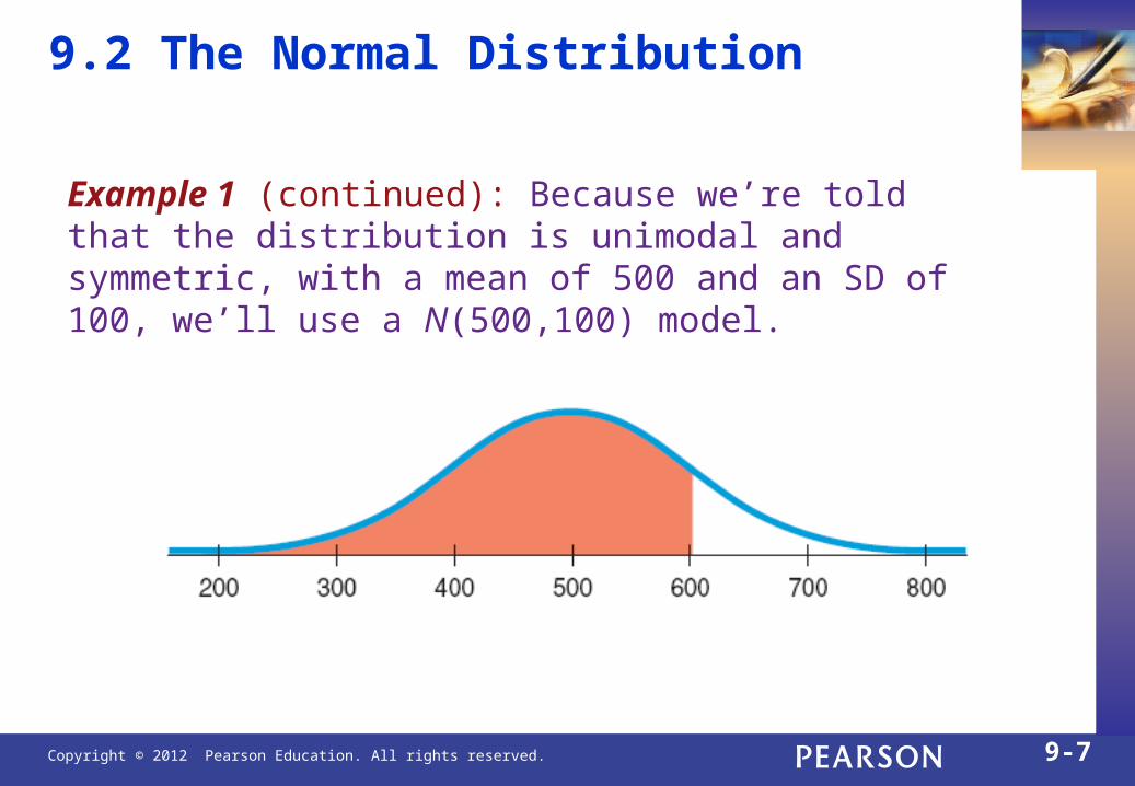
Example 1 (continued): Because we’re told that the distribution is unimodal and symmetric, with a mean of 500 and an SD of 100, we’ll use a N(500,100) model.
Copyright © 2012 Pearson Education. All rights reserved. 9-8
9.2 The Normal Distribution
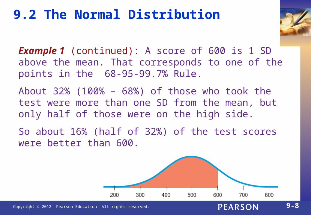
Example 1 (continued): A score of 600 is 1 SD above the mean. That corresponds to one of the points in the 68-95-99.7% Rule.
About 32% (100% – 68%) of those who took the test were more than one SD from the mean, but only half of those were on the high side.
So about 16% (half of 32%) of the test scores were better than 600.

Copyright © 2012 Pearson Education. All rights reserved. 9-9
9.2 The Normal Distribution
Example 2: Assuming the SAT scores are nearly normal with N(500,100), what proportion of SAT scores falls between 450 and 600?
Copyright © 2012 Pearson Education. All rights reserved. 9-10
9.2 The Normal Distribution
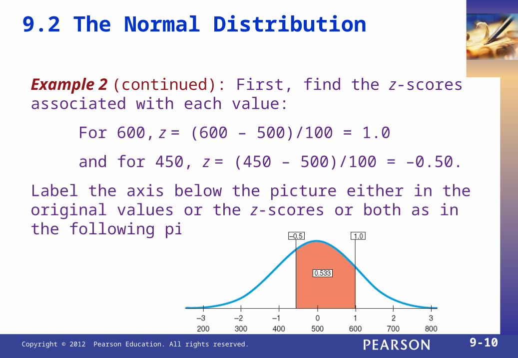
Example 2 (continued): First, find the z-scores associated with each value:
For 600, z = (600 – 500)/100 = 1.0
and for 450, z = (450 – 500)/100 = –0.50.
Label the axis below the picture either in the original values or the z-scores or both as in the following picture.
Copyright © 2012 Pearson Education. All rights reserved. 9-11
9.2 The Normal Distribution
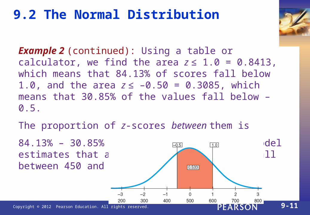
Example 2 (continued): Using a table or calculator, we find the area z ≤ 1.0 = 0.8413, which means that 84.13% of scores fall below 1.0, and the area z ≤ –0.50 = 0.3085, which means that 30.85% of the values fall below –0.5.
The proportion of z-scores between them is
84.13% – 30.85% = 53.28%. So, the Normal model estimates that about 53.3% of SAT scores fall between 450 and 600.
Copyright © 2012 Pearson Education. All rights reserved. 9-12
9.2 The Normal Distribution
Sometimes we start with areas and are asked to work backward to find the corresponding z-score or even the original data value.
Example 3: A college says it admits only people with SAT scores among the top 10%. How high an SAT score does it take to be eligible?
Copyright © 2012 Pearson Education. All rights reserved. 9-13
9.2 The Normal Distribution
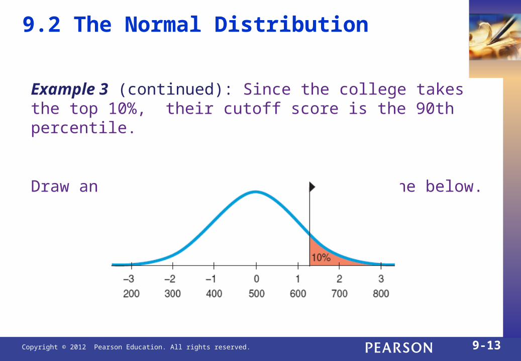
Example 3 (continued): Since the college takes the top 10%, their cutoff score is the 90th percentile.
Draw an approximate picture like the one below.
Copyright © 2012 Pearson Education. All rights reserved. 9-14
9.2 The Normal Distribution
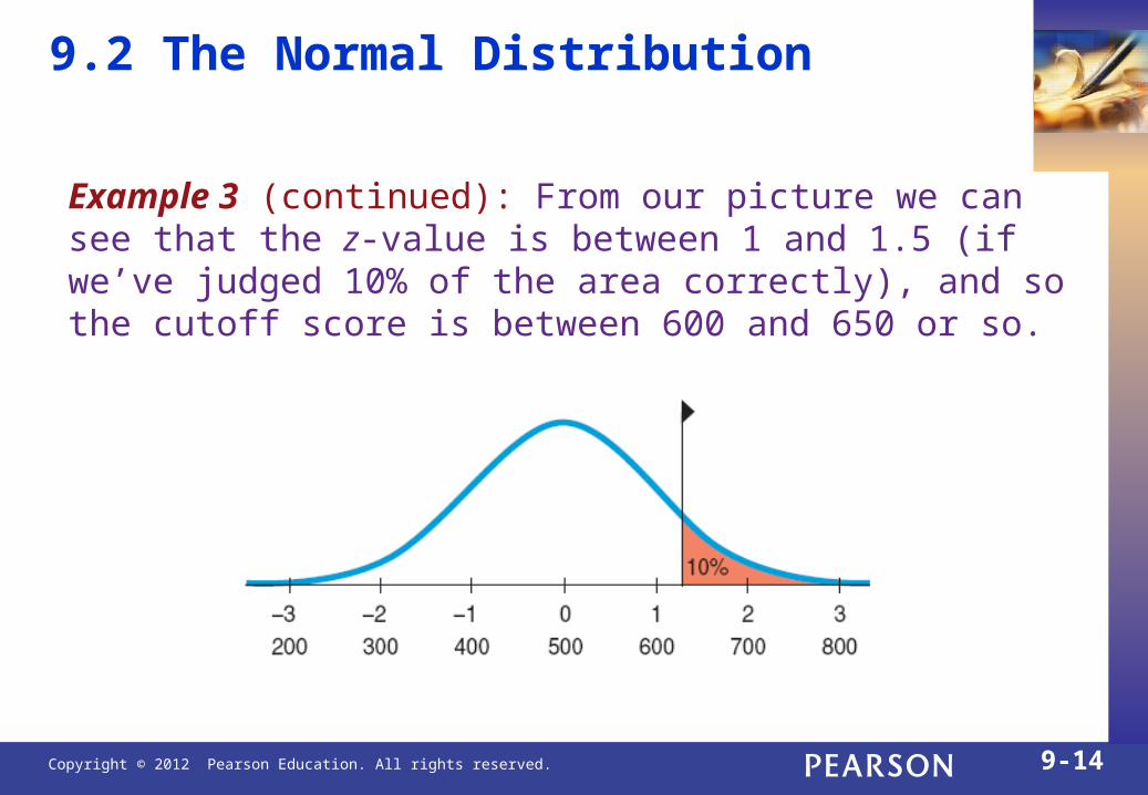
Example 3 (continued): From our picture we can see that the z-value is between 1 and 1.5 (if we’ve judged 10% of the area correctly), and so the cutoff score is between 600 and 650 or so.

Copyright © 2012 Pearson Education. All rights reserved. 9-15
9.2 The Normal Distribution
Example 3 (continued): Using technology, you may be able to select the 10% area and find the z-value directly.

Copyright © 2012 Pearson Education. All rights reserved. 9-16
9.2 The Normal Distribution
Example 3 (continued): If you need to use a table, such as the one below, locate 0.90 (or as close to it as you can; here 0.8997 is closer than 0.9015) in the interior of the table and find the corresponding z-score.
The 1.2 is in the left margin, and the 0.08 is in the margin above the entry. Putting them together gives z = 1.28.

Copyright © 2012 Pearson Education. All rights reserved. 9-17
9.2 The Normal Distribution
Example 3 (continued): Convert the z-score back to the original units.
A z-score of 1.28 is 1.28 standard deviations above the mean.
Since the standard deviation is 100, that’s 128 SAT points. The cutoff is 128 points above the mean of 500, or 628.
Since SAT scores are reported only in multiples of 10, you’d have to score at least a 630.
Copyright © 2012 Pearson Education. All rights reserved. 9-18
9.2 The Normal Distribution
Example: Tire Company
A tire manufacturer believes that the tread life of its snow tires can be described by a Normal model with a mean of 32,000 miles and a standard deviation of 2500 miles. If you buy a set of these tires, should you hope they’ll last 40,000 miles or more?

Copyright © 2012 Pearson Education. All rights reserved. 9-19
9.2 The Normal Distribution
Example: Tire Company
A tire manufacturer believes that the tread life of its snow tires can be described by a Normal model with a mean of 32,000 miles and a standard deviation of 2500 miles. If you buy a set of these tires, should you hope they’ll last 40,000 miles or more?
Since only 0.7% of all tires will last longer than 40,000 miles, it is not reasonable to expect that yours will.
40000 32000( 40000) ( 3.2) 0.0007
2500P y P z P z
Copyright © 2012 Pearson Education. All rights reserved. 9-20
9.2 The Normal Distribution
Example (continued): Tire CompanyA tire manufacturer believes that the tread life of its snow tires can be described by a Normal model with a mean of 32,000 miles and a standard deviation of 2500 miles. Approximately what percent of these snow tires will last less than 30,000 miles?
Copyright © 2012 Pearson Education. All rights reserved. 9-21
9.2 The Normal Distribution
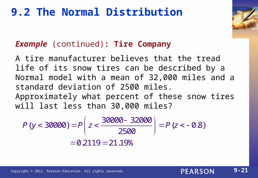
Example (continued): Tire Company
A tire manufacturer believes that the tread life of its snow tires can be described by a Normal model with a mean of 32,000 miles and a standard deviation of 2500 miles. Approximately what percent of these snow tires will last less than 30,000 miles?
30000 32000( 30000) ( 0.8)
2500
0.2119 21.19%
P y P z P z

Copyright © 2012 Pearson Education. All rights reserved. 9-22
9.2 The Normal Distribution
Example (continued): Tire Company
A tire manufacturer believes that the tread life of its snow tires can be described by a Normal model with a mean of 32,000 miles and a standard deviation of 2500 miles. Approximately what percent of these snow tires will last between 30,000 and 35,000 miles?

Copyright © 2012 Pearson Education. All rights reserved. 9-23
9.2 The Normal Distribution
Example (continued): Tire Company
A tire manufacturer believes that the tread life of its snow tires can be described by a Normal model with a mean of 32,000 miles and a standard deviation of 2500 miles. Approximately what percent of these snow tires will last between 30,000 and 35,000 miles?
30000 32000 35000 32000(30000 35000)
2500 2500
( 0.8 1.2) 0.6731 67.31%
P y P z
P z

Copyright © 2012 Pearson Education. All rights reserved. 9-24
9.2 The Normal Distribution
Example (continued): Tire Company
A tire manufacturer believes that the tread life of its snow tires can be described by a Normal model with a mean of 32,000 miles and a standard deviation of 2500 miles. A dealer wants to offer a refund to customers whose snow tires fail to reach a certain number of miles, but he can only offer this to no more than 1 out of 25 customers. What mileage can he guarantee?
Copyright © 2012 Pearson Education. All rights reserved. 9-25
9.2 The Normal Distribution
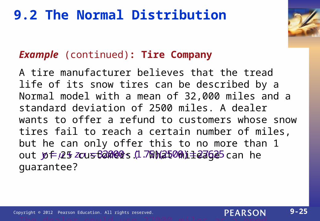
Example (continued): Tire Company
A tire manufacturer believes that the tread life of its snow tires can be described by a Normal model with a mean of 32,000 miles and a standard deviation of 2500 miles. A dealer wants to offer a refund to customers whose snow tires fail to reach a certain number of miles, but he can only offer this to no more than 1 out of 25 customers. What mileage can he guarantee?
The dealer could use 27000 miles as a good round number.
32000 (1.75)(2500) 27625y z
Copyright © 2012 Pearson Education. All rights reserved. 9-26
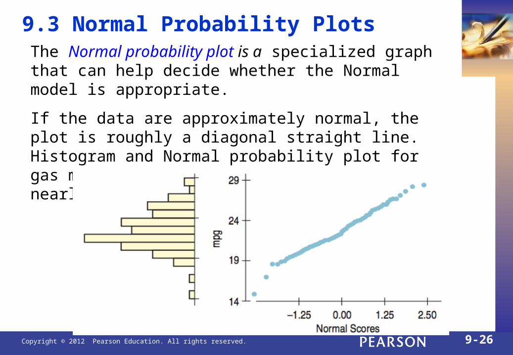
9.3 Normal Probability PlotsThe Normal probability plot is a specialized graph that can help decide whether the Normal model is appropriate.
If the data are approximately normal, the plot is roughly a diagonal straight line. Histogram and Normal probability plot for gas mileage (mpg) for a Nissan Maxima are nearly normal, with 2 trailing low values.
Copyright © 2012 Pearson Education. All rights reserved. 9-27
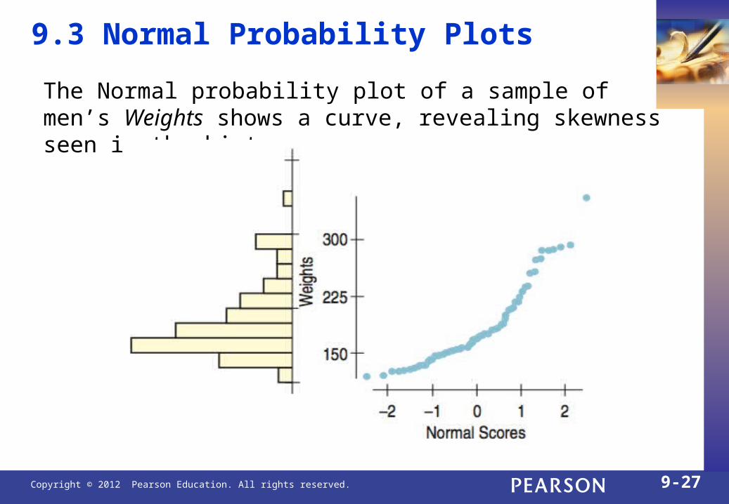
9.3 Normal Probability Plots
The Normal probability plot of a sample of men’s Weights shows a curve, revealing skewness seen in the histogram.
Copyright © 2012 Pearson Education. All rights reserved. 9-28
9.4 The Distribution of Sums of Normals
Normal models have many special properties. One of these is that the sum or difference of two independent Normal random variables is also Normal.

Copyright © 2012 Pearson Education. All rights reserved. 9-29
9.4
A company that manufactures small stereo systems uses a two-step packaging process. Stage 1 is combining all small parts into a single packet. Then the packet is sent to Stage 2 where it is boxed, closed, sealed and labeled for shipping. Stage 1 has a mean of 9 minutes and standard deviation of 1.5 minutes; Stage 2 has a mean of 6 minutes and standard deviation of 1 minutes. Since both stages are unimodal and symmetric, what is the probability that packing an order of two systems takes more than 20 minutes?

Copyright © 2012 Pearson Education. All rights reserved. 9-30
9.4
A company that manufactures small stereo systems uses a two-step packaging process. Since both stages are unimodal and symmetric, what is the probability that packing an order of two systems takes more than 20 minutes?
Normal Model Assumption - We are told both stages are unimodal and symmetric. And we know that the sum of two Normal random variables is also Normal.
Independence Assumption - It is reasonable to think the packing time for one system would not affect the packing time for the next system.
Copyright © 2012 Pearson Education. All rights reserved. 9-31
9.4
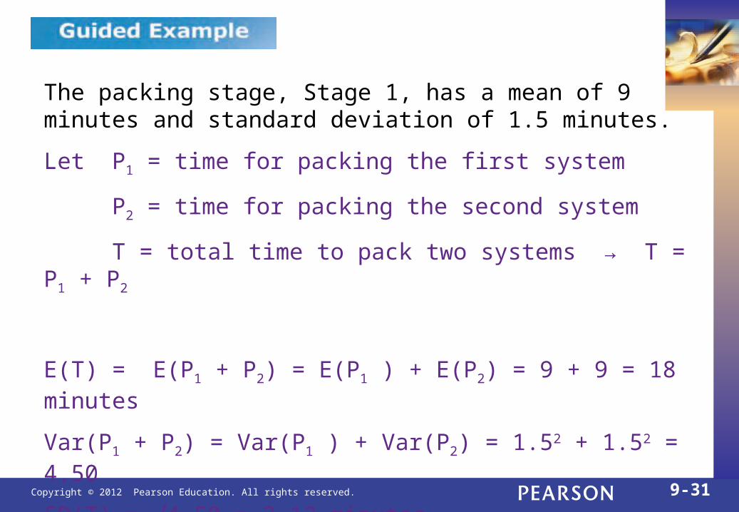
The packing stage, Stage 1, has a mean of 9 minutes and standard deviation of 1.5 minutes.
Let P1 = time for packing the first system
P2 = time for packing the second system
T = total time to pack two systems → T = P1 + P2
E(T) = E(P1 + P2) = E(P1 ) + E(P2) = 9 + 9 = 18 minutes
Var(P1 + P2) = Var(P1 ) + Var(P2) = 1.52 + 1.52 = 4.50
SD(T) = √4.50 = 2.12 minutes
We can model the time, T, with a N(18, 2.12) model.
Copyright © 2012 Pearson Education. All rights reserved. 9-32
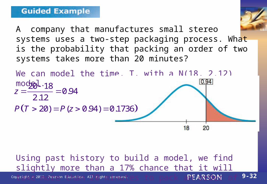
9.4A company that manufactures small stereo systems uses a two-step packaging process. What is the probability that packing an order of two systems takes more than 20 minutes?
We can model the time, T, with a N(18, 2.12) model.
Using past history to build a model, we find slightly more than a 17% chance that it will take more than 20 minutes to pack an order of two stereo systems.
20 180.94
2.1220) ( 0.94) 0.1736
z
P T P z

Copyright © 2012 Pearson Education. All rights reserved. 9-33
9.5 The Normal Approximation for the Binomial
A discrete Binomial model is approximately Normal if we expect at least 10 successes and 10 failures:
10 and 10np nq
Suppose the probability of finding a prize in a cereal box is 20%. If we open 50 boxes, then the number of prizes found is a Binomial distribution with mean of 10:
Note that the distribution is very nearly normal.

Copyright © 2012 Pearson Education. All rights reserved. 9-34
9.5 The Normal Approximation for the Binomial
For Binomial(50, 0.2),
10 and 2.83.
To estimate P(10):

Copyright © 2012 Pearson Education. All rights reserved. 9-35
9.6 Other Continuous Random VariablesA continuous random variable is a random variable that may take on any value in some interval [a, b].
The distribution of the probabilities can be shown with a curve, f (x) called a probability density function (pdf).
The standard Normal pdf:
Copyright © 2012 Pearson Education. All rights reserved. 9-36
9.6 Other Continuous Random Variables
Density functions must satisfy these requirements:
1) They must be non-negative for every possible value.
2) The area under the curve must exactly equal 1.

Copyright © 2012 Pearson Education. All rights reserved. 9-37
9.6 Other Continuous Random VariablesThe Uniform Distribution For values c and d
both within the interval [a, b]: c d
Expected Value and Variance:
Copyright © 2012 Pearson Education. All rights reserved. 9-38
9.6 Other Continuous Random Variables
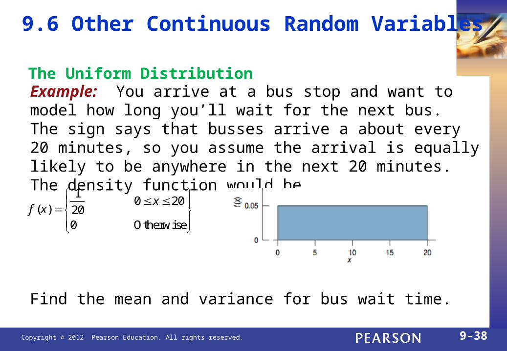
Example: You arrive at a bus stop and want to model how long you’ll wait for the next bus. The sign says that busses arrive a about every 20 minutes, so you assume the arrival is equally likely to be anywhere in the next 20 minutes. The density function would be
Find the mean and variance for bus wait time.
1 0 20
( ) 200 Otherwise
xf x
The Uniform Distribution
Copyright © 2012 Pearson Education. All rights reserved. 9-39
9.6 Other Continuous Random Variables
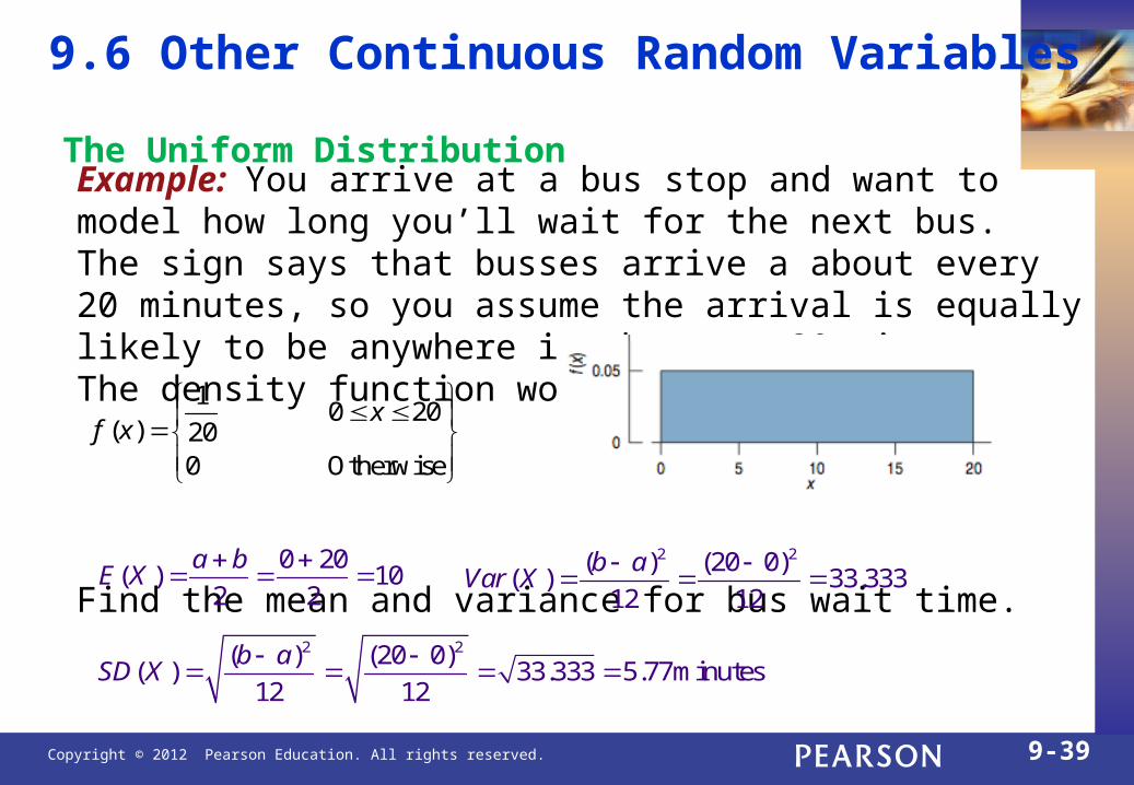
Example: You arrive at a bus stop and want to model how long you’ll wait for the next bus. The sign says that busses arrive a about every 20 minutes, so you assume the arrival is equally likely to be anywhere in the next 20 minutes. The density function would be
Find the mean and variance for bus wait time.
1 0 20
( ) 200 Otherwise
xf x
0 20( ) 10
2 2
a bE X
2 2( ) (20 0)( ) 33.333
12 12
b aVar X
2 2( ) (20 0)( ) 33.333 5.77minutes
12 12
b aSD X
The Uniform Distribution

Copyright © 2012 Pearson Education. All rights reserved. 9-40
9.6 Other Continuous Random VariablesThe Exponential Distribution
For modeling the time between events.

Copyright © 2012 Pearson Education. All rights reserved. 9-41
9.6 Other Continuous Random Variables
The Exponential Distribution
Example: If a website experiences 4 hits per minute, what is the probability that we will have to wait less than 20 seconds (1/3 minute) between two hits?
4 1/30 1/ 3 1 0.736P X e
We can expect to wait 20 seconds or less between hits about 75% of the time.

Copyright © 2012 Pearson Education. All rights reserved. 9-42
• Probability models are still just models.
• Don’t assume everything’s Normal.
• Don’t use the Normal approximation with small n.
Copyright © 2012 Pearson Education. All rights reserved. 9-43
What Have We Learned?
Recognize normally distributed data by making a histogram and checking whether it is unimodal, symmetric, and bell-shaped, or by making a normal probability plot using technology and checking whether the plot is roughly a straight line.
• The Normal model is a distribution that will be important for much of the rest of this course.
• Before using a Normal model, we should check that our data are plausibly from a normally distributed population.
• A Normal probability plot provides evidence that the data are Normally distributed if it is linear.
Copyright © 2012 Pearson Education. All rights reserved. 9-44
What Have We Learned?
Understand how to use the Normal model to judge whether a value is extreme.
• Standardize values to make z-scores and obtain a standard scale. Then refer to a standard Normal distribution.
• Use the 68–95–99.7 Rule as a rule-of-thumb to judge whether a value is extreme.
Know how to refer to tables or technology to find the probability of a value randomly selected from a Normal model falling in any interval.
• Know how to perform calculations about Normally distributed values and probabilities.
Copyright © 2012 Pearson Education. All rights reserved. 9-45
What Have We Learned?
Recognize when independent random Normal quantities are being added or subtracted.
• The sum or difference will also follow a Normal model
• The variance of the sum or difference will be the sum of the individual variances.
• The mean of the sum or difference will be the sum or difference, respectively, of the means.
Recognize when other continuous probability distributions are appropriate models.