coping with gray markets: the impact of market conditions

Acc

epte

d A

rtic

leAccepted ManuscriptTitle: Coping with Gray Markets: The Impact of Market Conditions andProduct Characteristics

Authors: Reza Ahmadi, Foad Iravani, Hamed Mamani

DOI: http://dx.doi.org/doi:10.1111/poms.12319

Reference: POMS 12319

To appear in: Production and Operations Management

Please cite this article as: Ahmadi Reza., et al.,

Coping with Gray Markets: The Impact of Market Conditions and Product Characteristics.

Production and Operations Management (2014), http://dx.doi.org/doi:10.1111/poms.12319

This article has been accepted for publication and undergone full peer review but has not

been through the copyediting, typesetting, pagination and proofreading process, which may

lead to differences between this version and the Version of Record. Please cite this article as

doi: 10.1111/poms.12319

Acc

epte

d A

rtic

leCoping with Gray Markets: The Impact of Market

Conditions and Product Characteristics

Reza Ahmadi∗

([email protected])Foad Iravani†

([email protected])Hamed Mamani†

([email protected])

September, 2014

Abstract

Gray markets, also known as parallel imports, have created fierce competition for manufac-turers in many industries. We analyze the impact of parallel importation on a price-setting man-ufacturer that serves two markets with uncertain demand, and characterize her policy againstparallel importation. We show that ignoring demand uncertainty can take a significant toll onthe manufacturer’s profit, highlighting the value of making price and quantity decisions jointly.We find that adjusting prices is more effective in controlling gray market activity than reducingproduct availability, and that parallel importation forces the manufacturer to reduce her pricegap while demand uncertainty forces her to lower prices. Furthermore, we explore the impact ofmarket conditions (such as market base, price sensitivity, and demand uncertainty) and productcharacteristics (”fashion” vs. ”commodity”) on the manufacturer’s policy towards parallel im-portation. We also provide managerial insights about the value of strategic decision-making bycomparing the optimal policy to the uniform pricing policy that has been adopted by some com-panies to eliminate gray markets entirely. The comparison indicates that the value of makingprice and quantity decisions strategically is highest for moderately different market conditionsand non-commodity products.

Keywords: gray markets, parallel importation, parallel markets, strategic pricing, demand un-certainty, uniform pricing.History: Received: February 2013, Revised: July 2013, January 2014, June 2014. Accepted:August 2014 by Amiya Chakravarty.

1 Introduction

Manufacturers around the world confront new pressures with the trade of their brand name products

in unauthorized distribution channels known as gray markets. Gray markets primarily emerge when

manufacturers offer their products in different markets at different prices. Price differentials may

motivate enterprises or individuals to buy products from authorized distributors in markets with

a lower price and sell them in markets with a higher price. Gray market channels may operate in

the same market as the authorized distributors, or bring parallel imports from another market.

∗Anderson School of Management, University of California, Los Angeles, 90095†Foster School of Business, University of Washington, Seattle, 98195

This article has been accepted for publication and undergone full peer review but has not been through the copyediting, typesetting, pagination and proofreading process, which may lead to differences between this version and the Version of Record. Please cite this article as doi: 10.1111/poms.12319

This article is protected by copyright. All rights reserved.

Acc

epte

d A

rtic

leEach year products worth billions of dollars are diverted to gray markets. In the IT industry

alone, the approximate value of gray market products was $58 billion dollars and accounted for

5 to 30 percent of total IT sales, according to a 2008 survey conducted jointly by KPMG and

The Alliance for Gray Market and Counterfeit Abatement (KPMG 2008). In the pharmaceutical

industry, 20% of the products sold in the United Kingdom are parallel imports (Kanavos and

Holmes, 2005). In communications, nearly 1 million iPhones were unlocked in 2007 and used

on unauthorized carriers worldwide (New York Times, 2008). International versions of college

textbooks, drinks, cigarettes, automobile parts, luxury watches, jewelry, electronics, chocolates,

and perfumes are among the numerous products that are traded in gray markets (Schonfeld, 2010).

Unlike counterfeits, products traded in gray markets are genuine. Growing numbers of efficient

global logistics networks help gray markets reach more customers faster. Advancing web technology

and a rapidly growing online retail sector also boost gray markets. Amazon, eBay, Alibaba, Kmart,

and Costco are among the retailers known to have sold gray goods (Bucklin, 1993; Schonfeld, 2010).

As to benefit and harm, opinions about gray markets are mixed. Manufacturers generally

consider gray markets harmful because products diverted to gray markets end up competing with

those sold by authorized distributors, and unauthorized channels get a free ride from expensive

advertising and other manufacturer efforts to increase sales. Also, brand value may erode as

products become available to segments that the manufacturer deliberately avoided. Gray markets,

however, can benefit manufacturers by generating extra demand and deterring competitors.

The existing literature on gray markets largely focuses on pricing decisions in deterministic

settings. While consumer demand can be accurately estimated for some products or markets, in

many cases manufacturers are challenged with high uncertainty in demand. In this paper, we

consider a manufacturer that operates in two markets with uncertain demand under the threat of

competition from a parallel importer. If the manufacturer were to charge different prices across

the markets, the parallel importer could buy the product in the low-price market and transfer it

to sell in the high-price market. The manufacturer can control gray market activities through two

operational levers: price and quantity. Consumers base their purchase decisions on prices offered

by the manufacturer and the parallel importer and their perception of the gray market relative to

the authorized channel.

Our paper makes three contributions to the literature. First, we extend the existing models

on parallel importation (e.g., Ahmadi and Yang, 2000; Xiao et al., 2011) to incorporate demand

uncertainty and quantity decisions in a Stackelberg game model. To the best of our knowledge, this


Acc

epte

d A

rtic

lepaper is the first work that analyzes both price and quantity decisions of a manufacturer that faces

parallel importation. The solution to the competition model determines the manufacturer’s reaction

to gray market activities, such as ignoring, allowing, or blocking parallel imports – referred to as

the manufacturer’s policy. Our analysis shows that the presence of parallel importation compels

the manufacturer to reduce her1 price gap, while uncertainty in demand compels her to reduce her

price in both markets. Moreover, reducing the price gap is more effective in controlling gray market

activity than creating scarcity in the low price market unless the manufacturer is better off exiting

the low price market completely. We show that ignoring demand uncertainty and using prices that

are optimal in a deterministic setting can severely hurt the manufacturer’s profit and result in a

suboptimal policy towards parallel importation; therefore, it is important to design a model that

accounts for both demand uncertainty and gray markets.

Our second contribution is that we explore the impact of market conditions and product charac-

teristics on the manufacturer’s policy. The term market conditions refers to relative market bases,

price sensitivities, and demand uncertainties, while the term product characteristics represents con-

sumers’ perception of parallel imports relative to the authorized channel. If consumers strongly

prefer to buy the product from the manufacturer, we refer to the product as a ”fashion” item,

whereas we refer to it as a ”commodity” when consumers are indifferent between buying from the

manufacturer and buying from the gray market. We observe that when the product is a fashion

item, the manufacturer mainly ignores the gray market. When the relative perception of parallel

imports is moderately high, meaning that the product is in transition from a fashion item to a

commodity, and market conditions are somewhat different, the manufacturer is better off allowing

parallel importation. Finally, when the product is a commodity and the competition from the par-

allel importer intensifies, the manufacturer’s policy is to block the gray market. These observations

provide guidelines for determining a company’s policy towards parallel importation.

Our third contribution is that we provide managerial insights about the value of making price

and quantity decisions strategically as opposed to using myopic policies in the presence of parallel

importation. In particular, we compare the manufacturer’s profit under the strategic pricing policy

to the profit of the myopic uniform pricing policy, which has been used by some companies, such

as TAG Heuer and Christian Dior (Antia et al., 2004). These international companies charge the

same price in all markets to eliminate price differentials and parallel importation entirely. Although

implementing a uniform pricing policy is easier, companies that adopt this policy forgo the benefit

1Throughout the paper, we refer to the manufacturer as a female and to the parallel importer as a male.


Acc

epte

d A

rtic

leof price discrimination in the strategic pricing policy. Our comparison shows that, on the one hand,

when market conditions are moderately different and the product has not become a commodity,

the additional profit of strategic pricing is significant and can be as high as 28%; therefore, it

is important that companies follow strategic pricing in these situations. On the other hand, we

observe that when market conditions are either too similar or too different and the product is a

commodity, uniform pricing becomes a good alternative to strategic pricing.

This paper is organized as follows. We review the literature in Section 2. In Section 3, we

describe the modeling framework and assumptions. Section 4 presents the main results of the

competition model and Section 5 discusses the observations and managerial insights. We conclude

the paper in Section 6 and offer directions for future work. Finally, the appendix explores some

extensions to our model such as the effects of exchange rate, correlated demand, and relaxing some

of the model assumptions.

2 Literature Review

Despite the ubiquity of gray markets, this topic occupies a relatively small niche in the interface of

marketing and operations management literature. Existing marketing and economics research into

gray markets can be divided into two groups of studies. The first group includes empirical studies

and qualitative discussions about factors leading to the emergence of gray markets, e.g., Dutta et

al. (1999), Maskus (2000), Ganslandt and Maskus (2004), and Antia et al. (2004).

The second group of studies includes analytical models for the price decision and whether or not

gray markets should be deterred. Dutta et al. (1994) study the optimal policy towards retailers

selling across their territories. Bucklin (1993) examines the claims made by trademark owners

and gray market dealers and draws public policy implications. Li and Maskus (2006) find that

parallel imports inhibit innovation and diminish welfare if the manufacturer deters parallel imports

with a high wholesale price. Matsushima and Matsumura (2010) and Chen (2009) explore the

ramifications of parallel imports for intellectual property holders and manufacturers. These studies

suggest that manufacturers should tolerate some level of territorial restriction violation. Xiao et

al. (2011) show that whether a manufacturer sells directly or through a retailer is critical to

determining the increase or reduction in manufacturer profit due to parallel importation. Shulman

(2013) shows that competing retailers may divert to gray markets even if it does not increase total

sales. Autrey et al. (2013) consider two firms that engage in a Cournot competition in a domestic


Acc

epte

d A

rtic

lemarket and face gray market activities when they enter a foreign market. They find that when the

products are close substitutes, it is better to decentralize the management structure in the foreign

market. Ahmadi and Yang (2000) investigate the interaction between a manufacturer and a parallel

importer in a deterministic setting with endogenous prices. They show that not only does parallel

importation increase total sales, but it can also increase manufacturer profit.

In the operations management literature, there exists a rich body of research on optimal pricing

and quantity decisions with stochastic demand (Petruzzi and Dada, 1999; Chan et al., 2004);

however, these studies ignore gray market activities. Recently, a few papers have analyzed quantity

decisions and coordination in supply chains that face gray markets. In these papers, however, either

price is exogenous or demand is deterministic. Dasu et al. (2012) consider a decentralized supply

chain with exogenous pricing in which a retailer could salvage leftover inventory or sell it to the

gray market. Altug and van Ryzin (2013) consider a manufacturer selling a product through a

large number of retailers that sell their excess inventory to a domestic gray market. They assume

a market-clearing price for the gray market, but an exogenous retail price. Hu et al. (2013) study

a reseller who takes advantage of a supplier quantity discount offer and diverts a portion of orders

to a gray market. They show that when the reseller’s batch inventory holding cost is high, the

gray market improves channel performance. Su and Mukhopadhyay (2012) consider a deterministic

setting in which a manufacturer offers a quantity discount to one dominant retailer and multiple

fringe retailers. Krishnan et al. (2013) study the impact of gray markets on a decentralized supply

chain with one manufacturer and two retailers that may divert the product to the gray market,

when demand is assumed to be deterministic.

Our work differs from the foregoing in that we analyze the impact of parallel importation

on a vertically integrated manufacturer who must set both prices and quantities before demand

uncertainty is resolved. We analyze the effect of market conditions and product characteristics on

the manufacturer’s policy and explore the value of a strategic reaction to parallel importation.

3 Modeling Assumptions and Framework

Consider a manufacturer who produces a single product at per-unit cost c and sells it in two separate

markets. The manufacturer chooses price p1 and quantity q1 in market 1, and chooses price p2 and

quantity q2 in market 2. We assume that there are no capacity constraints, and that unsatisfied

demand in both markets are lost. For ease of exposition, we assume holding costs, lost-sales costs,


Acc

epte

d A

rtic

le Table 1: NotationsParameters

Ni, bi, εi base, price sensitivity, and demand uncertainty of market i = 1, 2

(Li, Ui), µi, σi domain, expected value, and standard deviation of εi

fi(x), Fi (x) , hi (x) probability density, cumulative distribution, and hazard rate functions of εi

c manufacturer’s unit production cost

cG parallel importer’s unit transfer cost

δ consumer’s relative perception of parallel imports

Manufacturer’s Variables

pi, qi price and quantity in markets i = 1, 2

π expected total profit when there are no parallel imports

π expected total profit in the presence of the parallel importer

πd expected total profit in the presence of the parallel importer for deterministic demand

Manufacturer’s Optimal Variables

p̃i, q̃i when there are no parallel imports

p̃id, q̃i

d when there are no parallel imports and demand is deterministic

p∗i , q∗i in the presence of the parallel importer

p∗di , q∗di in the presence of the parallel importer for deterministic demand

Parallel Importer’s Variables

qG, pG, πG quantity, price, and profit

and salvage values are zero, though these parameters can be added to our model.

The demand in both markets is stochastic and depends on price. In particular, we assume

that demand in market i = 1, 2 is defined as Di (pi, εi) = di (pi) + εi = Ni − bipi + εi in which

di(pi) denotes the deterministic component of demand, Ni denotes the market base, bi denotes

the consumer sensitivity to price change (following Petruzzi and Dada, 1999; Ahmadi and Yang,

2000; Xiao et al., 2011; Su and Mukhopadhyay, 2012; Krishnan et al., 2013), and εi represents the

stochastic component of demand. We assume that εi takes its value in the interval (Li, Ui), and

denote the probability density and cumulative distribution functions of εi with fi(x) and Fi(x),

respectively. The expected value and the standard deviation of εi are denoted with µi and σi. We

assume that ε1 and ε2 are statistically independent and discuss the effect of correlated demands in

Appendix. We also assume that ε1 and ε2 satisfy the Increasing Failure Rate (IFR) property and

their hazard rate functions, denoted by hi(x) = fi(x)1−Fi(x) , is increasing; i.e., h′i(x) > 0. This property

holds for many common distributions such as normal and uniform (Lariviere and Porteus, 2001).

Table 1 summarizes the notations.

We analyze the competition between the manufacturer and a parallel importer using a Stack-


Acc

epte

d A

rtic

leelberg game model and the following sequence of events: (1) the manufacturer acts as the leader

and chooses her price and quantity for both markets before demand uncertainties are resolved;

(2) having observed manufacturer’s prices, the parallel importer may decide to buy the product

from the manufacturer in the low-price market and transfer to the high-price market for resale

if the price gap makes the venture sufficiently profitable. The parallel importer must choose the

quantity to buy from the manufacturer and set his selling price in the high-price market; (3) de-

mand uncertainty for the authorized channel is resolved in both markets and the total profits of

the manufacturer and the parallel importer (if he transfers the product) are realized.

We make two assumptions about the parallel importer for tractability. First, we assume that the

parallel importer places his order before other customers and the manufacturer cannot distinguish

the parallel importer’s order. Due to their economic incentives, most gray marketers hire agents

to swiftly purchase products. Also, in most situations it is very difficult for a manufacturer to

distinguish between orders received from customers who intend to buy the product for personal use

and orders placed by gray market agents, especially when orders are placed through the Internet.

KPMG’s survey of IT companies reports that 42% of the respondents do not have a process to

identify or monitor gray market activities, and that 62% of the respondents have no formal training

programs to educate their staff or customers about gray market issues. Antia et al. (2004) note that

methods for uncovering gray markets can be very costly and in many cases gray markets cannot be

identified and stopped completely as they counteract manufacturers’ efforts to track the diversion

of products to gray markets. In the appendix we discuss the effects of relaxing this assumption and

show that the outcomes of our model are fairly robust.

Our second assumption about the parallel importer is that he makes his decisions based on

an estimate of average demand and does not have the capability to estimate the uncertainty he

would face. We believe this assumption is reasonable because, unlike major manufacturers, most

gray marketers typically have low capital and cannot invest in market research to estimate the

parameters of demand distribution. Our numerical experiments in the appendix show that relaxing

this assumption has little impact on the main insights of our model.

Finally, we assume, without loss of generality, that the direction of parallel importation is from

market 1 to market 2. That is, if the manufacturer were able to achieve an ideal price discrimination

in the two markets without worrying about a gray market, then market 1 would be the low price

market and market 2 would be the high price market. To formalize this argument, let π represent

the manufacturer’s expected total profit if there were no parallel imports. Then the manufacturer


Acc

epte

d A

rtic

lesolves

maxp1,p2,q1,q2

π = Eε1,ε2

[p1min

{q1,D1 (p1, ε1)

}+ p2min

{q2,D2 (p2, ε2)

}− c(q1 + q2)

]. (1)

This is the classic price–setting newsvendor problem (Petruzzi and Dada, 1999) with two inde-

pendent markets. The optimal prices, p̃1 and p̃2, satisfy

Ni − 2bip̃i + zi (p̃i)−∫ zi(p̃i)

Li

Fi(x)dx+ cbi = 0 (i = 1, 2), (2)

in which zi (p̃i) = F−1i

(1− c

p̃i

)with F−1i (x) denoting the inverse of Fi(x). The optimal quantities

are equal to q̃i = di(p̃i) + zi (p̃i) (Xu et al., 2010). Throughout this paper, we assume that p̃2 > p̃1.

4 Analysis of Competition

We now assume that a parallel importer is present. By entering the high-price market (market 2),

the parallel importer engages in a Stackelberg game with the manufacturer. In what follows, we

use backward induction to characterize the equilibrium of this two-stage game.

4.1 Parallel Importer’s Problem

For given price and quantity decisions of the manufacturer, define qG to be the quantity that the

parallel importer buys from the manufacturer in market 1 and let pG be the gray market price in

market 2. We assume that the parallel importer incurs a cost of cG to transfer one unit of the

product to market 2. This cost represents the shipping cost and all other costs associated with

distributing the product in market 2 (e.g., translating the user manual, repackaging, tariffs).

When there are no parallel imports in market 2, some customers buy the product from the

manufacturer and some do not. Once the parallel importer enters market 2 and offers the product

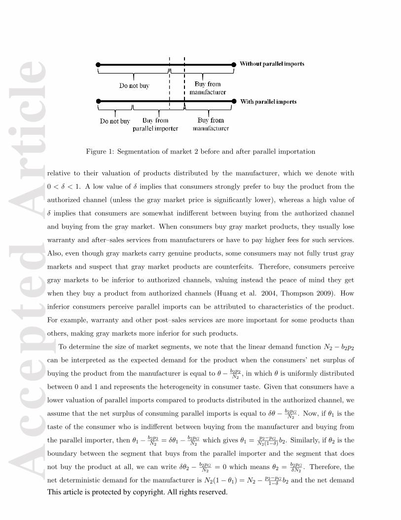
at price pG, the market divides into three segments as depicted in Figure 1. The first segment is

customers who continue to buy the product from the manufacturer. The second segment contains

customers who buy the product from the parallel importer. Some of these customers initially bought

from the manufacturer, but now switch to the parallel importer (the distance between the dashed

lines) and some had not considered buying the product before due to the higher price charged by

the authorized channel. The third segment contains those who had not bought the product before

and continue to refrain from doing so even after the parallel importer enters the market.

The size of these segments is determined by the prices set by the manufacturer and the parallel

importer. Size is also affected by the consumers’ perception (valuation) of gray–market products


Acc

epte

d A

rtic

le

Figure 1: Segmentation of market 2 before and after parallel importation

relative to their valuation of products distributed by the manufacturer, which we denote with

0 < δ < 1. A low value of δ implies that consumers strongly prefer to buy the product from the

authorized channel (unless the gray market price is significantly lower), whereas a high value of

δ implies that consumers are somewhat indifferent between buying from the authorized channel

and buying from the gray market. When consumers buy gray market products, they usually lose

warranty and after–sales services from manufacturers or have to pay higher fees for such services.

Also, even though gray markets carry genuine products, some consumers may not fully trust gray

markets and suspect that gray market products are counterfeits. Therefore, consumers perceive

gray markets to be inferior to authorized channels, valuing instead the peace of mind they get

when they buy a product from authorized channels (Huang et al. 2004, Thompson 2009). How

inferior consumers perceive parallel imports can be attributed to characteristics of the product.

For example, warranty and other post–sales services are more important for some products than

others, making gray markets more inferior for such products.

To determine the size of market segments, we note that the linear demand function N2 − b2p2

can be interpreted as the expected demand for the product when the consumers’ net surplus of

buying the product from the manufacturer is equal to θ− b2p2

N2, in which θ is uniformly distributed

between 0 and 1 and represents the heterogeneity in consumer taste. Given that consumers have a

lower valuation of parallel imports compared to products distributed in the authorized channel, we

assume that the net surplus of consuming parallel imports is equal to δθ − b2pGN2

. Now, if θ1 is the

taste of the consumer who is indifferent between buying from the manufacturer and buying from

the parallel importer, then θ1− b2p2

N2= δθ1− b2pG

N2which gives θ1 = p2−pG

N2(1−δ)b2. Similarly, if θ2 is the

boundary between the segment that buys from the parallel importer and the segment that does

not buy the product at all, we can write δθ2 − b2pGN2

= 0 which means θ2 = b2pGδN2

. Therefore, the

net deterministic demand for the manufacturer is N2(1− θ1) = N2 − p2−pG1−δ b2 and the net demand


Acc

epte

d A

rtic

lefor the parallel importer is N2(θ1 − θ2) = δp2−pG

δ(1−δ) b2. However, because the parallel importer buys

the product from the manufacturer in market 1, his order quantity is limited by q1. Therefore, the

parallel importer’s profit maximization problem is

maxpG

πG = (pG − p1 − cG) qG

in which qG = min(δp2−pGδ(1−δ) b2, q1

).

Proposition 1 For given prices p1 and p2, let ψ(p1, p2) = δp2−p1−cG2δ(1−δ) b2 be the parallel importer’s

desired quantity. If the manufacturer’s quantity in market 1 is large enough to fulfill the parallel

importer’s desired quantity, i.e., q1 > ψ(p1, p2), then the parallel importer’s optimal price and

quantity will be

pG =δp2 + p1 + cG

2, qG = max (0, ψ(p1, p2)) . (3)

Otherwise, pG = δp2 −δ(1− δ)q1

b2and qG = q1.

All proofs are provided in the supplementary document. Equation (3) shows the parallel im-

porter’s optimal decisions when he is not constrained by manufacturer’s quantity. The parallel

importer incurs a cost of p1 + cG to purchase the product in market 1 and transfer it to market 2.

Clearly, if this cost is above the manufacturer’s authorized price in market 2, p2, transferring the

product will not be profitable. However, because consumers in market 2 have a lower perception of

gray market products, the importer’s total purchase and transfer cost should be even lower (below

δp2) to justify his entry to the competition. As a result, the gray market is profitable if and only if

δp2 > p1 + cG. When product availability is low, the parallel importer charges pG = δp2 − δ(1−δ)q1b2

to sell q1.

4.2 Strategic Manufacturer’s Problem

Having obtained the parallel importer’s optimal decisions, we now find the manufacturer’s optimal

price and quantity decisions. In doing so, we also characterize the manufacturer’s optimal response

to gray market activities. Specifically, hereafter we make the following distinction between the

manufacturer’s decisions and her policy. We use decision to refer to the manufacturer’s price

and quantity values, and use policy to describe the manufacturer’s high-level reaction to parallel

importation. The manufacturer’s decisions can result in one of the following three policies:


Acc

epte

d A

rtic

leIgnore the parallel importer. Under this policy, the manufacturer continues to use her deci-

sions that are optimal in the absence of gray markets; i.e., p̃i and q̃i. We will later show that

the manufacturer uses this policy only if the gray market can be automatically eliminated by

using prices p̃1 and p̃2. Intuitively this would be the case when consumers’ relative perception

of parallel imports is very low (δ � 1) or the parallel importer’s transfer cost, cG, is so high

that it would be too costly for him to transfer the product. This policy also arises when p̃1

and p̃2 are fairly close to each other. In this situation, these prices would render the gray

market unprofitable unless δ is extremely high or cG is extremely small.

Block parallel imports. If the difference between p̃1 and p̃2 is large enough for the gray market to

operate, then the manufacturer may decide to block the parallel importer. The manufacturer

has two levers to block the gray market.

Block using prices. In this policy, the manufacturer blocks the gray market by altering her

prices such that δp2 = p1+cG. This could be an effective policy when the price difference

in the absence of gray markets (p̃2 − p̃1), consumers’ perception of parallel imports (δ),

and the importer’s transfer cost (cG) are such that the gray market could (barely) exist;

however, a small reduction in the price gap between the two markets could make parallel

importation no longer profitable. The manufacturer may also opt for this policy when

the parallel importer could emerge as a strong competitor. This can happen when the

consumers’ perception of parallel imports is very high. The gray market, if allowed,

could undercut the manufacturer and gain a significant portion of market 2.

Block using quantity. In this policy, the manufacturer blocks the gray market by making

the product unavailable to the parallel importer. Since there is usually no way of iden-

tifying the orders placed by parallel importers, this policy is equivalent to exiting (or

not entering) market 1. The manufacturer may choose this policy when the consumers’

perception of parallel imports is very high (δ ≈ 1) and the manufacturer’s optimal prices

in the absence of the gray market are significantly different across the markets (p̃1 � p̃2).

In this situation, the manufacturer would lose a significant portion of her profit if she

stays in both markets and blocks the gray market with prices. Therefore, she foregoes

the relatively small profit in market 1 to eliminate parallel importation and only oper-

ates in market 2 using price p̃2. The impact of parallel imports on market entry/exit

decisions has been witnessed by the pharmaceutical industry (2020health, 2011).


Acc

epte

d A

rtic

leAllow parallel imports. Under this policy, the manufacturer allows the parallel importer to

resell the product in market 2; i.e., she sets p1 and p2 such that δp2 − p1 − cG > 0, and

sets q1 > 0. The manufacturer would opt for this policy when p̃1 and p̃2 are moderately

different and the consumers’ perception of parallel imports is neither too high nor too low.

Blocking the parallel importer in such a setting requires a relatively significant deviation from

otherwise optimal decisions. Furthermore, because consumers still highly value the authorized

channel, the parallel importer is not a grave threat to the manufacturer. In this situation,

the manufacturer would allow the gray market to emerge simply because blocking the parallel

importer is more costly than allowing him.

The next proposition describes the impact of parallel imports on the manufacturer’s demand,

which has also been observed in deterministic settings (e.g., Ahmadi and Yang, 2000).

Proposition 2 When the parallel importer transfers the product, the manufacturer’s demand in

market 1 increases by qG, and her demand in market 2 decreases by δqG.

From Figure 1, we see that the manufacturer’s demand in market 2 reduces because some con-

sumers switch to the parallel importer. However, the segment of market 2 that buys the product

from the parallel importer increases the manufacturer’s demand in market 1. Overall, the manu-

facturer’s demand goes up because parallel importation provides the product at a lower price and

induces the consumers that have a lower willingness-to-pay to buy the product. The manufacturer

could directly offer the product at a discounted price, but doing so through the authorized channel

would lead to consumer confusion and severe demand cannibalization. Although the parallel im-

porter also cannibalizes the demand of the authorized channel, this effect is alleviated because the

importer is not affiliated with the manufacturer and has a lower reputation in the market.

To characterize the manufacturer’s optimal decisions and policy, we first present an interesting

result of our model. Proposition 1 states that the parallel importer ideally wants to transfer

ψ(p1, p2) = δp2−p1−cG2δ(1−δ) b2 units to market 2, but the actual quantity that he will obtain may be lower

than ψ(p1, p2) if q1 is small. However, the next proposition shows that the manufacturer will not

limit the parallel importer with quantity when she chooses prices that allow parallel importation.

Proposition 3 If the manufacturer’s prices (p1, p2) are such that the gray market could exist, i.e.,

δp2 − p1 − cG > 0, then the optimal policy of the manufacturer is to either (a) block the parallel

importer using quantity; i.e., q∗1 = 0, or (b) allow the parallel importer and provide a large enough

quantity in market 1 to fulfill his entire order; i.e., q∗1 ≥ ψ(p1, p2).


Acc

epte

d A

rtic

leThis proposition suggests that a mixed policy of allowing gray market activities through prices,

but limiting the size of the gray market through quantity (i.e., allowing partial importation) is not

optimal. Put differently, once she decides to allow gray market activities, the manufacturer would

not reduce product availability to limit parallel importation. We note that this result depends on

our assumption that the parallel importer is the first customer who receives the product. However,

our experiments in the appendix indicate that even if this assumption is relaxed, the manufacturer

will not limit the gray market by reducing her quantity. That is, prices are more effective in

controlling gray market activities than reducing product availability.

We can now formulate the Stochastic Stackelberg Game (SSG) to characterize the manufac-

turer’s optimal decisions and policy

maxp1,p2,q1,q2

π = Eε1,ε2

[p1min {q1,D1 (p1, ε1) + qG(p1, p2)}

+ p2min {q2,D2 (p2, ε2)− δqG(p1, p2)} − c(q1 + q2)], (4)

where qG(p1, p2) = max(0, ψ(p1, p2)) in light of Proposition 3. The next proposition characterizes

the solution to the SSG.

Proposition 4 Suppose the manufacturer does not leave market 1. Let p̂1 be the solution to the

following equation

δ

(N1 − 2b1p̂1 + cb1 + z1 (p̂1)−

∫ z1(p̂1)

L1

F1(x)dx

)

+N2 − 2b2

(p̂1 + cG

δ

)+ cb2 + z2

(p̂1 + cG

δ

)−∫ z2

(p̂1+cGδ

)L2

F2(x)dx = 0. (5)

Then, p̂1 is unique and

(a) If δp̃2 − p̃1 − cG ≤ 0, then the manufacturer’s optimal policy is to ignore the parallel importer.

Thus, p∗1 = p̃1 and p∗2 = p̃2.

(b) If δp̃2 − p̃1 − cG > 0 and η > 0, where

η = N1 − 2b1p̂1 +cG

2δ (1− δ)b2 + z1 (p̂1) + c

(b1 +

b22δ

)−∫ z1(p̂1)

L1

F1 (x) dx, (6)

then the optimal policy is to block the parallel importer by setting p∗1 = p̂1 and p∗2 = p̂1+cGδ .


Acc

epte

d A

rtic

le(c) If δp̃2 − p̃1 − cG > 0 and η ≤ 0, then it is optimal to allow parallel importation. In this case,

p∗1 and p∗2 satisfy the following equations:

N1 − 2b1p∗1 +

2 (δp∗2 − p∗1)− cG2δ (1− δ)

b2 + c

(b1 +

b22δ

)+ z1 (p∗1)−

∫ z1(p∗1)

L1

F1 (x) dx = 0,

N2 − 2b2p∗2 −

2 (δp∗2 − p∗1)− cG2 (1− δ)

b2 + cb22

+ z2 (p∗2)−∫ z2(p∗2)

L2

F2 (x) dx = 0.

(d) The manufacturer’s optimal quantities are

q∗1 = d1 (p∗1) + qG (p∗1, p∗2) + z1 (p∗1) , q∗2 = d2 (p∗2)− δqG (p∗1, p

∗2) + z2 (p∗2) .

The manufacturer controls the parallel importer’s order quantity through her prices. However,

changing the prices also affects the demand of the authorized channels. Therefore, she should

choose prices that balance these effects. For given prices p1 and p2, if the parallel importer is

allowed to transfer the product, then the change in the manufacturer’s expected total profit will

be (p1 − δp2 − c(1 − δ))qG(p1, p2), which is negative because the importer would enter only if

δp2 − p1 > cG. This means that, while total demand increases according to Proposition 2, the

manufacturer’s profit would always be less in the presence of the parallel importer. Thus, if p̃1 and

p̃2 happen to eliminate the importer (i.e., δp̃2− p̃1− cG ≤ 0), then the manufacturer simply ignores

the parallel importer.

When δp̃2 − p̃1 − cG > 0, the manufacturer has to change her prices and deviate from p̃1 and

p̃2. In this scenario, the optimal policy would be to either block the parallel importer (by setting

δp2− p1− cG = 0), or to allow him (by setting δp2− p1− cG > 0). Thus, one can solve the SSG by

imposing the constraint δp2 − p1 − cG ≥ 0. The parameter η defined in (6) is simply the shadow

price of this constraint for (p̂1,p̂1+cGδ ). Proposition 4 shows that the optimal blocking price, p̂1, and

its corresponding shadow price, η, are the factors that determine whether the optimal policy is to

allow or block the parallel importer. If p̂1 makes the corresponding shadow price positive, then the

constraint will be tight and the manufacturer will block the importer via p̂1 and p̂1+cGδ . However,

if the shadow price is non-positive, then allowing parallel importation is the optimal policy.

We note that when δ approaches 1, (6) is positive and the manufacturer will always block the

parallel importer. In this situation, products in the gray market become perfect substitutes for

products in the authorized channel and the competition is highly intense. Therefore, the parallel

importer could gain a significant size of market 2 if allowed.


Acc

epte

d A

rtic

leCorollary 1 If consumers’ relative perception of parallel imports is very high, i.e., if δ ≈ 1, then

the manufacturer blocks parallel importation.

Proposition 4 assumes that the manufacturer is better off staying in both markets. The following

result provides a necessary condition for when it is better for the manufacturer to exit (not enter)

market 1 and only operate in market 2.

Proposition 5 If the optimal policy for the manufacturer is to block the parallel importer with

quantity (leave market 1) for given model parameters, then N1 − b1 (δp̃2 − cG) + z1 (δp̃2 − cG) ≤ 0.

The interpretation of this necessary condition is that δp̃2 − cG must be too high to generate a

positive demand (hence a positive quantity) in market 1. Otherwise, the manufacturer can increase

her profit by selling the product at price δp̃2 − cG in market 1 and still block parallel importation.

Next we look at how the presence of the parallel importer changes the manufacturer’s prices.

Proposition 6 If the presence of the parallel importer forces the manufacturer to alter her other-

wise optimal prices (i.e., δp̃2 − p̃1 − cG > 0), then the manufacturer always increases her price in

market 1 and reduces her price in market 2. That is, p∗1 > p̃1 and p∗2 < p̃2.

The presence of the parallel importer forces the manufacturer to reduce her price gap, whether

she allows or blocks parallel imports. When the manufacturer allows the importer to transfer the

product, she increases her price in market 1 because the importer generates extra demand in that

market. The manufacturer also reduces her price in market 2 because of the competition from the

parallel importer in that market. If the manufacturer’s policy is to block the importer, she has to

choose prices so that δp2 − p1 − cG = 0. Doing so by increasing p1 or reducing p2 alone severely

hurts the manufacturer’s profit in the authorized channels. Therefore, she reduces the price gap by

adjusting p1 upward and p2 downward.

Next, we analyze the effect of demand uncertainty on the manufacturer’s prices when she faces

parallel imports. For this purpose, we define the DSG as the deterministic version of the SSG in

which ε1 and ε2 are replaced with their expected values, µ1 and µ2, as follows

(DSG) maxp1,p2

πd =(pd1 − c

)(D1

(pd1, µ1

)+ qG(p1, p2)

)+(pd2 − c

)(D2

(pd2, µ2

)− δqG(p1, p2)

).

Let p∗d1 and p∗d2 denote the solution to the DSG and define q∗d1 = N1 + µ1 − b1p∗d1 and q∗d2 =

N2 + µ2 − b2p∗d2 . The next proposition compares the prices of the SSG to those of the DSG.


Acc

epte

d A

rtic

leProposition 7 Given the same average demand, the optimal prices in the stochastic demand case

(SSG) are always less than the optimal prices when demand is assumed to be deterministic (DSG);

i.e., p∗1 < p∗d1 and p∗2 < p∗d2 .

Prior work has shown a similar result for a single market with additive uncertainty in the

absence of parallel importation. For example, Petruzzi and Dada (1999) show that the optimal

price of a price-setting newsvendor who serves a single market is always below the optimal price

when demand is equal to the average of the stochastic demand. Proposition 7 extends this result

to the setting in which two markets are connected by parallel importation. We note that this result

holds regardless of the policies adopted by the manufacturer under the SSG and DSG scenarios.

Proposition 6 shows that the existence of a gray market forces the manufacturer to increase

p1 and reduce p2. In order to make a similar comparison between the quantities released in each

market, we note that parallel importation influences the manufacturer’s quantities in two ways.

First, it increases the demand in market 1 by qG(p1, p2) and decreases the demand in market 2 by

δqG(p1, p2). Thus, the manufacturer would like to increase q1 and decrease q2 accordingly. Second,

given the directions of price change in Proposition 6, the demand of the authorized channel in

market 1 decreases while the demand of the authorized channel in market 2 increases. While

we were not able to prove the magnitude of these effects analytically, our extensive numerical

experiments indicated that the second effect proves to be stronger. Consequently, in the presence

of a gray market, the manufacturer keeps a lower quantity in market 1 and a higher quantity in

market 2. We can prove this result analytically when demand is deterministic in both markets.

Proposition 8 In the DSG, the optimal quantity in market 1 (market 2) in the presence of parallel

imports is less (greater) than the optimal quantity when there are no parallel imports, i.e., q∗d1 < q̃1d

and q∗d2 > q̃2d.

Ahmadi and Yang (2000) made the same observation when the manufacturer selects the block

policy. We show that the same direction of changes is valid regardless of the policy.

5 Discussion and Managerial Insights

This section presents numerical experiments that respond to the motivating questions raised in

the introduction. We first highlight the value of developing a model that jointly incorporates the

competition from parallel importers and demand uncertainty. We then provide managerial insights


Acc

epte

d A

rtic

lethat can help address some policy questions of interest to manufacturers, such as the transition

of the optimal policy as model parameters vary, and the value of strategic decision-making in the

presence of a gray market.

Table 2 lists the parameter values of the experiments. N1 and N2 values were chosen between

1, 000 and 10, 000 to capture markets with approximately same size (N1/N2 = 1) as well as markets

with significantly different sizes (N2/N1 = 1/10 and N2/N1 = 10). b1 and b2 varied from 1 to 4 to

represent markets with very similar sensitivity to price (b1/b2 = 1) and markets with very different

sensitivity to price (b2/b1 = 1/4 and b2/b1 = 4). We chose equidistant values from each range

to keep the total number of experiments manageable. We set the manufacturer’s production cost

to 250 and 550, a low and high production cost relative to market bases. The sample data in Li

and Maskus (2006) suggests that transport costs to and import duties of the United States range

from 3% to 10% of FOB value2 for most products. In our model, we are only concerned with the

parallel importer’s transfer cost and not his shipping mode. Therefore, we set cG to 3% and 10% of

c. We assumed ε1 and ε2 to have the same distribution, but not necessarily the same parameters.

We focused on normal and uniform distributions as they are widely used in the literature (e.g.,

Schweitzer and Cachon, 2000; Yao et al., 2006). Because the behaviors we observed for the uniform

distribution were not significantly different from those for the normal distribution, we only present

the results for the normal distribution. We set µi to 0.1Ni and changed σi such that the coefficient

of variation of εi was 0.5, 1, and 2. When running the experiments, we considered all parameter

combinations except those that resulted in market 1 price being greater than or equal to market 2

price, violating the direction of import. Therefore, we considered 4490 cases for our experiments.

5.1 Value of a Joint Model

We have developed a unified framework to analyze the decisions of a manufacturer that faces

gray market activities and uncertain demand. As pointed out in the literature review, prior work

in marketing and operations management largely dealt with price and quantity decisions in the

presence of either a parallel importer or uncertain demand. Our model studies the simultaneous

effects of both parallel importation and demand uncertainty.

2FOB is an acronym for Free on Board. It is a type of sea transport contract in which the seller pays for

transportation of the goods to the port of shipment, plus loading costs. The buyer pays cost of marine freight

transport, insurance, unloading, and transportation from the arrival port to the final destination. The passing of

risks occurs when the goods are loaded on board at the port of shipment (http://www.iccwbo.org).


Acc

epte

d A

rtic

le Table 2: Parameter values for numerical experiments

Ni (i = 1, 2) {1, 000, 4, 000, 7, 000, 10, 000}

bi (i = 1, 2) {1, 2, 3, 4}

µi (i = 1, 2) 0.1Ni

σi (i = 1, 2) {0.5µi, µi, 2µi}

c {250, 550}

cG {0.03 c, 0.1 c}

5.1.1 Cost of Ignoring Parallel Importation

In the first set of experiments, we looked at how much profit the manufacturer would forfeit if

she does not take into consideration the possibility of parallel importation and treats each market

separately. In our experiments, we observed that the magnitude of profit losses can be as high as

70%, depending on the consumers’ perception of parallel imports. Figure 2(a) is an example of our

experiments and shows the percentage of the manufacturer’s profit loss when she continues to use

p̃1 and p̃2 for different values of δ and σ1 = σ2 = σ, when N1 = N2 = 1, 000, b1 = 3, b2 = 2, c = 250,

and cG = 25. When δ is very low, parallel importation is not a threat and there is no profit loss.

As δ increases, however, the profit loss increases. Even for relatively moderate values of δ, the

manufacturer can lose between 10% to 20% of her profit if she does not take the parallel importer

into account. For larger values of δ, profit losses reach 60%.

5.1.2 Cost of Ignoring Demand Uncertainty

We also evaluated the profit loss to the manufacturer when she is aware of the presence of the

parallel importer, but does not take demand uncertainty into consideration. For this purpose,

we first solved the DSG and obtained its optimal solution, (p∗d1 , p∗d2 , q

∗d1 , q

∗d2 ). We then evaluated

the profit of the SSG for the optimal deterministic decisions. In our test set, we observed that the

reduction in the manufacturer’s profit can be as high as 57% depending on the magnitude of demand

uncertainty. When consumers’ relative perception of parallel imports is very high, the percentage

of profit loss decreases in δ because the price gap becomes narrower both in the deterministic model

and in the stochastic model. One exception to this behavior for very high values of δ, however, is

when the market parameters dictate that the manufacturer exit market 1 in the stochastic model,


Acc

epte

d A

rtic

le

50

100

150

200

0.550.650.750.850.95

0

20

40

60

80

σ

δ

(a) Error percentage of using p̃1 and p̃2 as a heuristic so-

lution for the SSG.

50

100

150

200

0.550.650.750.850.95

20

40

60

σ

δ

(b) Error percentage of using the solution to the DSG as

a heuristic solution for the SSG.

Figure 2: Error percentage of ignoring parallel imports or demand uncertainty.

while the optimal policy in the deterministic model is to stay in both markets. In this situation,

the percentage of profit loss increases in δ. Figure 2(b) illustrates one example of our experiments

when N1 = N2 = 1, 000, b1 = 3, b2 = 2, c = 250, and cG = 25 in which ignoring demand uncertainty

is detrimental to the manufacturer and she could lose as much as 57% of her profit. Therefore, it

is crucial that manufacturers account for both uncertainty in demand and parallel importation in

making price and quantity decisions.

5.2 How Do Market Conditions and Product Characteristics Determine Policy?

Though determining the optimal price and quantity decisions of the manufacturer has been the main

objective of our model, an important high-level question for any manufacturer is: What is the best

policy to cope with the gray market? In this section, we examine the manufacturer’s optimal

policy through the lens of two important dimensions of our model: product-specific parameters

and market-specific parameters, of which an important one is demand uncertainty in each market.

More specifically, we define market conditions as the aggregate effect of market-based parame-

ters, such as standard deviation of demand uncertainties, market bases, and price sensitivities. We

say market conditions are “similar” (“different”) if the parameters of the markets are such that

the price gap would naturally be small (large) even if there were no parallel imports; i.e., small

(large) p̃2 − p̃1.


Acc

epte

d A

rtic

leThe parameter that represents product characteristics in our model is δ. A low value of δ means

that parallel imports and authorized-channel products are quite distinct in the eyes of consumers,

whereas a very high value of δ means that consumers’ valuations of the gray market and the

authorized channel are very close. The higher the δ, the more intense the competition between

the manufacturer and the parallel importer. We define “commodity” items as products for which

consumers have a relatively high perception of parallel imports and are almost indifferent between

the authorized channel and the gray market (i.e., δ ≈ 1). At the other end of the spectrum, we define

“fashion” items as products for which consumers have a relatively low perception of parallel imports

(δ � 1) and strongly prefer to buy the product from the authorized channel. We emphasize that

the term “fashion” does not necessarily refer to the brand of the product in our context. Rather, we

use this term (and “commodity”) to concisely convey the degree of consumers’ inclination towards

the authorized channel. The factors that can influence the perception of parallel imports include

the maturity of the product, consumers’ knowledge of and familiarity with the product, and the

risks associated with buying from the gray market.

Figure 3 depicts the simultaneous effects of product characteristics (δ) and market conditions

on the regions characterizing the optimal policy when N1 = N2 = 4, 000, b1 = 2, b2 = 1, c = 550,

and cG = 55. To further highlight the effect of demand uncertainty, Figure 3a illustrates the

optimal policies when demand in market 2 is known (σ2 = 0), whereas Figure 3b demonstrates

the same when demand in market 1 is deterministic (σ1 = 0). In both graphs, the horizontal axis

represents the product characteristic, ranging from fashion to commodity from left to right; the

vertical axis represents the standard deviation of demand in the market with uncertain demand

(as a measure of market conditions ranging from “similar” to “different”). Note that in Figure 3a,

the bottom row corresponds to σ1 = 0; given that σ2 = 0 as well, this row represents prior work in

the literature that assumes deterministic demand in both markets. If demand in market 1 becomes

variable (σ1 > 0), a special case of Proposition 7 indicates that p̃1 < p̃ d1 . Given that σ2 = 0 (and

p̃2 = p̃ d2 ), inclusion of demand variability in market 1 means more “different” market conditions

between markets 1 and 2 (i.e., p̃2 − p̃1 > p̃ d2 − p̃ d1 ). Note that the values of σ2 in Figure 3b are

sorted in the reverse order of σ1 values in Figure 3a. This is because if demand in market 2 becomes

variable, then p̃2 < p̃ d2 . Given that σ1 = 0, inclusion of demand variability in market 2 means more

“similar” market conditions between markets 1 and 2 (p̃2 − p̃1 < p̃ d2 − p̃ d1 ). Note that the top row

in Figure 3b is same as the bottom row in Figure 3a.

First, we observe the same pattern in both graphs. When the product is a fashion item and


Acc

epte

d A

rtic

leIg

nor

e

Blo

ckBlock

Blo

ckBlock

Allow

δ

σ10.55 1

2.5µ

2µ

1.5µ

µ

0.5µ

0

(a) σ2 = 0

Ign

ore

Blo

ckB

lock Allow

Blo

ckB

lock

δ

σ20.58

0.73

0.93 1

0

0.5µ

µ

1.5µ

2µ

2.5µ

“D

iffere

nt”

Mark

et

Condit

ions

“Sim

ilar”

(b) σ1 = 0

Figure 3: Effects of demand uncertainty and product characteristics on manufacturer’s policy

market conditions are somewhat similar, the manufacturer can ignore the parallel importer. As

parallel imports gain acceptance from consumers and/or market conditions somewhat differ, the

manufacturer’s policy is to block the parallel importer by slightly deviating from her otherwise

optimal decisions. When there is a higher perception of parallel imports or when market conditions

are moderately different, it is no longer beneficial for the manufacturer to block the gray market,

as it requires large deviations from her otherwise optimal decisions in each market. In this region,

parallel imports are allowed into market 2. Finally, when the product is a commodity or when

market conditions are significantly different, the manufacturer goes back to blocking the parallel

importer. We note that the gray market can be blocked with price or quantity. In our experiments,

we observed that blocking with quantity may arise only when the market conditions are vastly

different and the product is a commodity.

Second, Figure 3 readily shows the impact of demand uncertainty on the manufacturer’s optimal

policy towards parallel importation. As demand uncertainty increases in either market, the manu-

facturer may change her policy from block to allow and/or from allow to block. This observation

shows that ignoring demand uncertainty not only may have a significant impact on the manufac-

turer’s profit, as illustrated in Section 5.1.2, but it may also affect her optimal policy towards the

gray market; the manufacturer may block (or allow) parallel importation when it is not optimal to

do so. Finally, we note that the effect of demand uncertainty in the two markets are not the same.

Increasing demand variability in market 1 makes the two markets more different, while increasing

demand variability in market 2 renders the two markets more similar.

While Figure 3 plots the optimal policy regions for when demand uncertainty is chosen as a


Acc

epte

d A

rtic

leproxy for market conditions, we observe a similar behavior when market bases or price sensitivities

are used to represent market conditions.

5.3 Strategic Versus Uniform Pricing

Implementing the optimal price and quantity decisions prescribed by the SSG requires estimating

the value of parameters, such as the relative perception of parallel imports, δ, and the parallel

importer’s transfer cost, cG, among others specific to the gray market. Antia et al. (2004) report

that some manufacturers have adopted a uniform pricing policy and charge the same price for

their products across all markets to eliminate gray markets entirely. The uniform pricing policy

requires less information and facilitates price coordination. Nevertheless, this policy bears the risk

of fluctuations in exchange rates and the manufacturer parts with the added profit from using the

market-specific prices that the SSG provides.

We conducted experiments to provide insights into the impact of market conditions and product

characteristics on the extra profit the manufacturer would earn by using the SSG recommendations.

The optimal uniform price, pu, can be obtained by solving (1), while enforcing p1 = p2. Figure 4

represents a common behavior we observed in our experiments where N1 = N2 = 10, 000, b2 = 1,

c = 250, cG = 25, and σ1 = σ2 = 2, 000. It illustrates the ratio of the manufacturer’s profit

under the SSG to her profit under the uniform pricing policy as a function of δ for various market

conditions captured with relative price sensitivities, b1/b2. We observed the same behavior when

market conditions were represented by other market parameters.

We observe two important behaviors in Figure 4. First, despite the benefits of the uniform

pricing policy such as easier implementation, there is a large range of δ and market conditions in

which the manufacturer’s profit will be significantly higher, as high as 28%, if she uses strategic

prices rather than using a uniform price. Therefore, in many situations it is indeed crucial that

companies put effort into market research to obtain the necessary information for strategic pricing.

The second observation is that the benefit of strategic pricing is greatest when market conditions

are not too similar or too different, namely they are moderately different, and the product has not

turned to a commodity. The ratio of profits decreases with δ and when b1/b2 = 4 and δ is high,

the ratio equals one. Also, when δ is sufficiently below one, the additional profit from strategic

pricing is higher for b1/b2 = 3 (moderately different market conditions) than for b1/b2 = 2 (similar

market conditions) and b1/b2 = 4 (different market conditions). The reason for this pattern is that

when market conditions are very similar, the price gap in the absence of parallel imports, p̃2− p̃1, is


Acc

epte

d A

rtic

le

0 0.2 0.4 0.6 0.8 11

1.05

1.1

1.15

1.2

1.25

1.3

δ

b1b2

= 2b1b2

= 3b1b2

= 4

Figure 4: Ratio of optimal profit in the SSG to the uniform pricing profit

naturally small and the manufacturer blocks the parallel importer with prices for most values of δ.

Since p̃1 ≤ pu ≤ p̃2 and p̃2 − p̃1 is small, the manufacturer will not lose too much if she charges pu

in both markets. When market conditions are very different, the manufacturer would not be able

to charge a single price that attracts significant portions of both markets simultaneously. Thus,

pu = p̃2 and the manufacturer leaves market 1 for the sake of the higher profit in market 2. For

strategic pricing, although the manufacturer has the opportunity to boost her profit by charging

markets differently, if she stays in both markets, she will have to charge very different prices. The

parallel importer will exploit the high price gap and transfer a large amount of the product, reducing

the manufacturer’s profit in market 2. As a result, the small profit from market 1 no longer pays

off the loss of profit to the parallel importer in market 2, especially when δ is very high and the

product is a commodity. Therefore, the manufacturer eventually decides to only operate in market

2, which means that the strategic and uniform pricing policies become identical.

In summary, we find that strategic pricing leads to a significant increase in profits for non-

commodity products when the two markets are moderately different. In extreme cases, however,

when markets are either too similar or too different and the product is a commodity, the uniform

pricing policy can be considered a viable alternative to strategic pricing.


Acc

epte

d A

rtic

le6 Conclusion

In this paper, we analyzed the impact of parallel importation on a manufacturer’s price and quantity

decisions in an uncertain environment, and showed that reducing the price gap is more effective in

controlling the gray market than reducing product availability. We found that the manufacturer’s

policy depends heavily on market conditions and product characteristics. When the product is a

fashion item, the manufacturer mainly ignores the parallel importer. The manufacturer blocks the

parallel importer when the product is a commodity. In that case, she may be forced to leave (or not

enter) the less profitable market and only serve the more profitable market. Finally, if the product

is in transition from a fashion item to a commodity, the manufacturer allows the parallel importer

to operate if the market conditions are moderately different.

We also showed that strategic pricing is indeed significantly more valuable than a uniform pricing

policy when the product is not a commodity and market conditions are moderately different. Thus,

in these situations it is worth investing in market studies to have a better understanding of market

parameters and consumer’s perception of gray goods, and to set prices strategically. However, if

market conditions are too similar or too different and the product is a commodity, uniform pricing

is a good alternative to strategic pricing.

Some of the assumptions made throughout this paper can be relaxed to extend the model in

several directions; these extensions are summarized here and discussed further in the appendix.

First, our framework enables us to include the uncertainty in exchange rate between the two

markets, which can be an important factor in international gray market activities. Second, our

model can be extended to allow for demand correlation between the two markets. Specifically,

we show that when demands follow a bivariate normal distribution, and the manufacturer can

use the demand signal in market 1 to set her quantity decision for market 2, she earns higher

profit and is more tolerant of parallel importation when markets are highly correlated. Third, our

model assumes that the parallel importer places and receives his order before other customers; this

assumption directly affects Proposition 3 and the results thereafter. In reality, it is likely that

the authorized channel and parallel importer’s demand are satisfied concurrently. When demand

from both channels are fulfilled proportionally, our numerical results indicate that the statement

of Proposition 3 and the qualitative nature of our results still hold true. Fourth, we assumed that

the parallel importer’s demand is perceived to be deterministic. In general, our numerical results

illustrate that variability in parallel importer’s demand reduces the manufacturer’s profit because


Acc

epte

d A

rtic

lethe parallel importer acts conservatively and sets a lower price. Furthermore, we find the effect of

relaxing the deterministic demand assumption on our model and the insights to be minimal.

Our work has limitations that can be addressed in future research. It would be interesting

to analyze the impact of parallel importation on the manufacturer in a multi-period setting. We

assume that the manufacturer has unlimited capacity. Limited capacity can impact the manufac-

turer’s allocation of quantities to each market, which then changes her prices. Also, because the

importer can act as an agent who transfers the product between markets, he can influence the

manufacturer’s capacity investment decisions, especially when capacity costs are different across

the markets. We leave these extensions for future research.

Acknowledgments

The authors are grateful for suggestions made by the anonymous reviewers, associate editor, and

department editor throughout the review process.

References

2020health. 2011. Parallel importing and exporting of pharmaceuticals severely limits the options in designing

an effective UK drug pricing scheme. (November 15), http://2020health.wordpress.com

Ahmadi, R., B. R. Yang. 2000. Parallel imports: Challenges from unauthorized distribution channels. Mar-

keting Science. 19(3) 279–294.

Altug, M., G. van Ryzin. 2013. Supply chain efficiency and contracting in the presence of gray market.

Working paper.

Antia, K. D., S. Dutta, M. Bergen. 2004. Competing with gray markets. Sloan Management Review. 46(1)

63-69.

Autrey, R. L., F. Bova., D. Soberman. 2013. Organizational structure and gray markets. Working paper.

Bucklin, L. P. 1993. Modeling the international gray market for public policy decisions. International Journal

of Research in Marketing. 10 387-405.

Cachon, G. P., M. A. Lariviere. 1999a. Capacity choice and allocation: Strategic behavior and supply chain

performance. Management Science. 45(8) 1091–1108.

Cachon, G. P., M. A. Lariviere. 1999b. An equilibrium analysis of linear, proportional and uniform allocation

of scarce capacity. IIE Transactions. 31 835–849.


Acc

epte

d A

rtic

leChan, L. M. A., Z. J. M. Shen, D. Simchi-Levi, J. Swann. 2004. Coordination of pricing and inventory

decisions: A survey and classification. Handbook of Quantitative Supply Chain Analysis: Modeling in

the E-Business Era. D. Simchi-Levi, S. D. Wu, Z. J. M. Shen. Kluwer Academic Publishers. 335-392.

Chen, H. 2009. Gray marketing: Does it hurt the manufacturers? Atlantic Economic Journal. 37(1) 23–35.

Dasu, S., R. Ahmadi, S. Carr. 2012. Gray markets: A product of demand uncertainty and excess inventory.

Production Operations Management. 21(6) 1102–1113.

Dutta, S., M. Bergen, G. John. 1994. The governance of exclusive territories when dealers can bootleg.

Marketing Science. 13(1) 83–99.

Dutta, S., J. B. Heide, M. Bergen. 1999. Vertical territorial restrictions and public policy: Theories and

industry evidence. Journal of Marketing. 63 121–134.

Ganslandt, G., K. E. Maskus. 2004. Parallel imports and the pricing of pharmaceutical products: Evidence

from the European Union. Journal of Health Economics. 23(5) 1035-1057.

Hines, W. W., D. C. Montgomery. 1990. Probability and Statistics in Engineering and Management Science.

J. Wiley, New York.

Hu, M., M. Pavlin., M. Shi. 2013. When gray markets have silver linings: All-unit discounts, gray markets

and channel management. Manufacturing Service Oper. Management. 15(2) 250-262.

Huang, J., B. C.Y. Lee., S. H. Ho. 2004. Consumer attitude toward gray market goods. International Mar-

keting Review. 21(6) 598–614.

Kanavos, P., P. Holmes. 2005. Pharmaceutical Parallel Trade in the U.K. The Institute for the Study of Civil

Society. London, U.K.

KPMG. 2008. Effective channel management is critical in combating the gray-market and increasing tech-

nology companies bottom line. http://www.agmaglobal.org.

Krishnan, H., J. Shao., T. McCormick. 2013. Impact of gray markets on a decentralized supply chain.

Working paper.

Lariviere, M. A., E. L. Porteus. 2001. Selling to a newsvendor: An analysis of price-only contracts. Manu-

facturing Service Oper. Management. 3(4) 293-305.

Li, C., K. E. Maskus. 2006. The impact of parallel imports on investments in cost-reducing research and

development. Journal of International Economics. 68 443-455.

Maskus, K. E. 2000. Parallel imports. World Economy. 23(9) 1269-1284.

Matsushima, N., T. Matsumura. 2010. Profit-enhancing parallel imports. Open Economics Review. 21(3)

433–447.

Petruzzi N. C., M. Dada. 1999. Pricing and the Newsvendor Problem: A review with extensions. Operations

Research. 47(2) 183–194.


Acc

epte

d A

rtic

leSchonfeld, M. 2010. Fighting grey goods with trademark law. Managing Intellectual Property. http://www.

pancommunications.com/_docs/burnslevinson20100601.pdf

Schweitzer, M. E., G. P. Cachon. 2000. Decision bias in the newsvendor problem with a known demand

distribution: Experimental evidence. Management Sci. 46(3) 404–420.

Shulman, J. D. 2013. Product diversion to a direct competitor. Working paper.

Su X., S. K. Mukhopadhyay. 2012. Controlling power retailer’s gray activities through contract design.

Production Operations Management. 21(1) 145–160.

Thompson, S. 2009. Gray power: An empirical investigation of the impact of parallel imports on market

prices. J. Ind. Compet. Trade 9(3) 219–232.

Xiao, Y., U. Palekar., Y. Liu. 2011. Shades of gray – The impact of gray markets on authorzied distribution

channels. Quantitative Marketing and Economics. 9 155–178.

Xu, M., Y. Chen., X. Xu. 2010. The effect of demand uncertainty in a price-setting newsvendor model.

European Journal of Operational Research. 207(2) 946–957.

Yao, L., Y. Chen, H. Yan. 2006. The newsvendor problem with pricing: Extensions. International Journal

of Management Science and Engineering Management. 1(1) 3–16.

Appendix. Model Extensions

Exchange Rate Uncertainty and Market–Specific Production Costs

We have assumed that the manufacturer produces the product at cost c and releases it in the

markets. A manufacturer may produce her product at local facilities. Also, the exchange rate

between the markets may be uncertain. We are able to incorporate both market–specific production

costs and exchange rate uncertainty into our model. Suppose c1 and c2 denote the production cost

in markets 1 and 2, respectively, and the exchange rate in market 2 is a random variable r with

expected value µr, which is resolved after both the manufacturer and the parallel importer set their

decisions. Then the parallel importer’s problem changes to

maxpG

πG = Er [(rpG − p1 − cG) qG] = (µr pG − p1 − cG) qG. (7)

Propositions 2–3 continue to hold and qG(p1, p2) = max(0, ψ(p1, p2)), but ψ(p1, p2) = µrδp2−p1−cG2δ(1−δ)µr b2

and the entry condition for the parallel importer changes to µrδp2−p1−cG > 0. The manufacturer’s


Acc

epte

d A

rtic

leprofit–maximization problem in the SSG changes to

maxp1,p2,q1,q2

π = Eε1,ε2

[p1min {q1,D1 (p1, ε1) + qG(p1, p2)} − c1q1

+ µrp2min {q2,D2 (p2, ε2)− δqG(p1, p2)} − µrc2q2]. (8)

We can characterize the optimal decisions and policy of the manufacturer by making appropriate

adjustments for c1, c2, and µr in Proposition 4. We omit the details due to limited space.

One can consider an alternative sequence of events where the manufacturer defers her pricing

decisions until after the exchange rate uncertainty is resolved. Under this scenario, the model

evolves to a three-stage game: The manufacturer makes her quantity decisions in stage 1; Having

observed exchange rate r, the manufacturer sets her pricing decisions in stage 2; The gray market

imports the product from market 1 to market 2 in stage 3. We can modify our framework to

consider this sequence of events as follows. In stage 3, the gray market solves a problem similar

to (7) where µr is replaced by r. In stage 2, the manufacturer solves a problem similar to (8)

where µr is replaced by r and optimization is taken over p1 and p2 only. Finally, in stage 1 the

manufacturer maximizes her expected total profit similar to (8) where p1 and p2 are replaced by

their solutions from stage 2, µr is replaced by r, the expectation is taken over ε1 and ε2 as well

as r, and optimization is taken over q1 and q2. We leave further analysis of gray market activities

under exchange rate uncertainty with alternative sequence of events for future research.

Correlated Demand

Suppose that demand uncertainties, ε1 and ε2, are correlated and let ζ(ε1, ε2) be the joint probability

density function and ρ represent the correlation of ε1 and ε2. Then our analysis continues to

work if fi(x) and Fi(x) represent the marginal probability density and distribution functions of

εi, i.e., f1(x) =∫ U2

ε2=L2ζ(x, ε2)d ε2 and f2(x) =

∫ U1

ε1=L1ζ(ε1, x)d ε1. This is true because the total

expected profit of the manufacturer is the sum of the expected profit in each market. In particular,

when ζ(ε1, ε2) is a bivariate normal distribution with means µ1, µ2, standard deviations σ1, σ2, and

correlation ρ, we have ε1 ∼ N(µ1, σ

21

)and ε2 ∼ N

(µ2, σ

22

)(Hines and Montgomery, 1990, p. 217);

therefore, demand correlation does not alter the optimal decisions of the manufacturer.

To make demand correlation effective in the case of bivariate normal distribution, we consider an

alternative sequence of events which is similar to the current sequence except that the manufacturer

determines q2 after ε1 is resolved. Under this sequence, the manufacturer observes ε1 and uses the

correlation between ε1 and ε2 to decide what quantity of the product she wants to release in market


Acc

epte

d A

rtic

le2. We still assume that the manufacturer determines both p1 and p2 before uncertainties are resolved

because the parallel importer can make his decisions only when both prices are announced. For

this alternative sequence of events, the manufacturer solves

maxp1,p2,q1,q2

π = Eε1 [p1 min {q1,D1 (p1, ε1) + qG(p1, p2)} − cq1 + π2(ε1)] ,

The term π2(ε1) = Eε2 [p2 min {q2, N2 − b2p2 − δqG(p1, p2) + ε2|ε1} − cq2] is the manufacturer’s ex-

pected profit in market 2 given the realized uncertainty in market 1.

Using the properties of the bivariate normal distribution, ε2|ε1=ε1 has a normal distribution

with mean µ2 + ρσ2σ1

(ε1 − µ1) and standard deviation σ2√

1− ρ2 (Hines and Montgomery, 1990, p.

218). Let φ(x) and Φ(x) denote the density and cumulative distribution functions of the standard

normal distribution. Propositions 2–3 are independent of correlation and remain intact. Therefore,

given prices (p1, p2) and ε1, the optimal quantities will be q∗1 = d1 (p1) + qG (p1, p2) +µ1 + z1 (p1)σ1

and q∗2 = d2 (p2) − δqG (p1, p2) + µ2 + ρσ2σ1

(ε1 − µ1) + z2 (p2)σ2√

1− ρ2. Substituting the optimal

quantities and using the property of the normal distribution, the manufacturer’s total expected

profit is π = (p1−c)(d1(p1)+qG (p1, p2)+µ1)−p1φ (z1 (p1))σ1+(p2−c2) (d2(p2)− δqG (p1, p2) + µ2)−

p2φ (z2 (p2))σ2√

1− ρ2.

Therefore, we can find the optimal prices by using Proposition 4 with F1(x) being a normal

distribution function with parameters µ1 and σ1 and F2(x) being a normal distribution function with

parameters µ2 and σ2√

1− ρ2. We repeated our experiments to explore the effect of correlation.

We found the price in market 2, and therefore the price gap, is higher for larger values of |ρ|.

Note that this observation is in line with Proposition 7, which states that prices get lower with

uncertainty. When the correlation between two markets is high, the demand in market 2 is more

predictable and closer to the deterministic demand case; therefore, the price of market 2 (and the

price gap as a result) is higher when demand is highly correlated across the two markets. As a

result the quantity and profit of the parallel importer are nondecreasing in |ρ|. Nevertheless, the

manufacturer’s profit is increasing in |ρ| since the manufacturer sets q2 after observing ε1 and the

higher the absolute value of the correlation, the lower the demand variability in market 2.

Demand Fulfillment

We now investigate the effect of relaxing our assumption that the parallel importer obtains the

product before customers in the authorized channel. Suppose δp2 − p1 − cG > 0 and the parallel

importer wishes to transfer the product. If the manufacturer’s quantity in market 1 is greater


Acc

epte

d A

rtic

lethan the sum of the realized authorized channel demand and the parallel importer’s ideal order

quantity, i.e., q1 ≥ d1(p1) + ε1 +ψ(p1, p2), where ε1 is a realization of ε1, then the parallel importer

can transfer ψ(p1, p2) to market 2. However, if q1 < d1(p1) + ε1 + ψ(p1, p2) and supply is less

than total demand, then we assume that the quantities obtained by the authorized channel and the

parallel importer are proportional to the size of their orders. Specifically, the authorized channel

will obtain(

d1(p1)+ε1d1(p1)+ε1+ψ(p1,p2)

)q1 units and the parallel importer will obtain

(ψ(p1,p2)

d1(p1)+ε1+ψ(p1,p2)

)q1

units. A similar proportional allocation policy has been used in the supplier capacity assignment

literature such as Cachon and Lariviere (1999a and 1999b).

Given ε1, the parallel importer’s optimal price and manufacturer’s best response q1 can be found.

However, finding p∗1, p∗2, and q∗2 in closed form is not possible because the change in manufacturer’s

demand in market 2 depends on optimal pG which in turn depends on the realization of ε1. So

in order to analyze the effect of this assumption we resort to numerical experiments. We find

p∗1, p∗2, q∗2 using Monte Carlo simulation–optimization, sampling 5,000 values of ε1 and ε2 in each

iteration. More specifically, we use Matlab optimization toolbox to find the values of (p1, p2, q2)

that maximize the average of the total profit for 5,000 values of demand uncertainty.

Table 3 illustrates a typical observation in our experiments. Mixed demand fulfillment refers

to the proportional splitting scenario. The value of p∗1 (p∗2) when the parallel importer obtains the

product first provides an upper (lower) bound for p∗1 (p∗2) in the mixed fulfillment setting. This is

because competition from the gray market becomes weaker when the parallel importer only obtains

a proportion of short supply. Therefore, the manufacturer can afford to increase the price gap

across the two markets by lowering p1 and increasing p2. The case of δ = 0.7 shows an interesting

situation in which the parallel importer is blocked when he obtains the product first; however, the

manufacturer allows some gray market activity when demand fulfillment is mixed. Furthermore,

q∗1 is higher when demand fulfillment is mixed and, more importantly, it is still higher than the

parallel importer’s ideal order quantity, which is ψ(p∗1, p∗2). Therefore, our numerical experiments

indicate that the statement in Proposition 3 holds true even when the parallel importer may not

be able to obtain the product before customers in the authorized channel.

Finally, we note that the manufacturer’s profit under the two cases are fairly close. Overall, we

observed a profit loss of less than 2% in most of our experiments. Therefore, while significantly

simplifying model analysis, the assumption that the parallel importer obtains the product first does

not appear to significantly affect the outcomes.


Acc

epte

d A

rtic

le Table 3: Effect of mixed demand fulfillmentImporter’s demand is fulfilled first Mixed demand fulfillment

δ p∗1 p∗2 q∗1 qG(p∗1, p∗2) Mfg. profit p∗1 p∗2 q∗1 qG(p∗1, p

∗2) Mfg. Profit

0.6 518 904 571 0 530015 518 904 571 0 530015

0.7 563 840 495 0 519771 561 845 512 13 520832

0.8 591 785 483 37 498601 588 794 524 71 501444

0.9 616 725 464 61 470549 615 735 523 118 473202

Uncertainty in Parallel Importer’s Demand

So far, we have assumed that the parallel importer’s demand is deterministic (or more precisely he

perceives his demand to be deterministic). Suppose that the parallel importer’s demand is defined

as DG(p2, pG, εG) = dG(p2, pG)+ εG, where dG(p2, pG) = δp2−pGδ(1−δ) b2 and εG is a random variable with

distribution function FG(x) defined on (LG, UG), expected value µG, and standard deviation σG.

Then, the parallel importer solves the following problem

maxpG,qG

πG = EεG [pGmin {qG, DG(p2, pG, εG)} − (p1 + cG)qG] ,

and his optimal price and quantity decisions satisfy the following optimality equations

(δp2 − 2pG) + p1 + cGδ(1− δ)

b2 + zG(pG)−∫ zG(pG)

LG

FG(x)dx = 0,

qG =δp2 − pGδ(1− δ)

b2 + zG(pG), zG(pG) = F−1G

(1− p1 + cG

pG

).

Since the optimal decisions of the parallel importer do not have a closed form, we are not able to

characterize the solution to the SSG analytically. We repeated our numerical experiments assuming

that the parallel importer also faces uncertain demand. Our experiments indicate that although

uncertainty in parallel importer’s demand changes the values of equilibrium decisions, it does not

impact the qualitative nature of our observations and managerial insights. Interestingly, we observe

that uncertainty in the parallel importer’s demand reduces the manufacturer’s profit. This is be-

cause the parallel importer acts conservatively and sets a lower price when his demand is uncertain,

which in turn creates a stronger competition for the manufacturer in market 2. Nevertheless, the

profit loss for the manufacturer was on average 3% and at most 5% in our experiments.


coping with gray markets: the impact of market conditions

Documents