coordination of resources across areas for the integration

Coordination of Resources acrossAreas for the Integration of

Renewable Generation: Operation,Sizing, and Siting of Storage Devices

Submitted in partial fulfillment of the requirements for

the degree ofDoctor of Philosophy

in

Electrical and Computer Engineering

Kyri Baker

B.Sc., Electrical and Computer Engineering, Carnegie Mellon University

M.Sc., Electrical and Computer Engineering, Carnegie Mellon University

Carnegie Mellon University

Pittsburgh, PA

December 2014

Keywords: Optimal Power Flow, Energy Storage, Distributed Optimization, ChanceConstraints, Model Predictive Control, Renewable Energy Integration

To my parents.

Abstract

An increased penetration of renewable energy into the electric power grid is desirable

from an environmental standpoint as well as an economical one. However, renewable

sources such as wind and solar energy are often intermittent, and additionally, are non-

dispatchable. Also, the locations with the highest amount of available wind or solar may

be located in areas that are far from areas with high levels of demand, and these areas may

be under the control of separate, individual entities. In this dissertation, a method that

coordinates these areas, accounts for this intermittency, reduces the impact of renewable

energy forecast errors, and increases the overall social benefit in the system is developed.

The approach for the purpose of integrating intermittent energy sources into the electric

power grid is considered from both the planning and operations stages. In the planning

stage, two-stage stochastic optimization is employed to find the optimal size and location

for a storage device in a transmission system with the goal of reducing generation costs,

increasing the penetration of wind energy, alleviating line congestions, and decreasing the

impact of errors in wind forecasts. The size of this problem grows dramatically with

respect to the number of variables and constraints considered. Thus, a scenario reduction

approach is developed which makes this stochastic problem computationally feasible. This

scenario reduction technique is derived from observations about the relationship between

the variance of locational marginal prices corresponding to the power balance equations

and the optimal storage size.

Additionally, a probabilistic, or chance, constrained model predictive control (MPC)

v

problem is formulated to take into account wind forecast errors in the optimal storage sizing

problem. A probability distribution of wind forecast errors is formed and incorporated

into the original storage sizing problem. An analytical form of this constraint is derived to

directly solve the optimization problem without having to use Monte-Carlo simulations or

other techniques that sample the probability distribution of forecast errors.

In the operations stage, a MPC AC Optimal Power Flow problem is decomposed with

respect to physical control areas. Each area performs an independent optimization and

variable values on the border buses between areas are exchanged at each Newton-Raphson

iteration. Two modifications to the Approximate Newton Directions (AND)method are

presented and used to solve the distributed MPC optimization problem, both with the

intention of improving the original AND method by improving upon the convergence rate.

Methods are developed to account for numerical difficulties encountered by these formula-

tions, specifically with regards to Jacobian singularities introduced due to the intertemporal

constraints.

Simulation results show convergence of the decomposed optimization problem to the

centralized result, demonstrating the benefits of coordinating control areas in the IEEE 57-

bus test system. The benefit of energy storage in MPC formulations is also demonstrated in

the simulations, reducing the impact of the fluctuations in the power supply introduced by

intermittent sources by coordinating resources across control areas. An overall reduction

of generation costs and increase in renewable penetration in the system is observed, with

promising results to effectively and efficiently integrate renewable resources into the electric

power grid on a large scale.

vi

Acknowledgments

The research presented in this thesis would not have been possible without the contributions

and support of the following people: To my parents, who have provided me with love,

support, and understanding throughout my life and especially throughout my PhD. To

Gabriela Hug, for giving me such a valuable opportunity, for always holding me up to high

standards, and for providing the prototype for what a good professor should be. To Xin

Li, for sharing his optimization knowledge and for his perceptive observations, and to my

thesis committee members Jeremy Michalek and Santiago Grijalva, for their insight and

expert opinions.

Thank you to the National Science Foundation, the National Energy Technology Labo-

ratory, and the SYSU-CMU Joint Institute of Engineering for making this research possible.

To Milos, for the metal concerts, for the many adventures and laughs, and for the deep

philosophical conversations. To Cristina, for being there for me when I was down, and for

providing interesting viewpoints on any issue. To Becky, for being an amazing roommate

and friend, and for helping me keep calm and carry on. To JY, my first friend in the office,

who was always very supportive, fun, and made me feel welcome. To Javad, for all of the

times we’ve made fun of each other, for being honest, and for being a true friend. To Max,

for all the hilarious moments we’ve enjoyed, and for all of the restaurant recommendations.

To Malika, for keeping it real. To Jon, for all the conversations about research ideas, and

all of the racquetball matches. To Shaurya, for all of the encouraging words, support, and

robots.

vii

To Erica, Paul, Ross, Skanda and Abe: I will never forget the fun times we’ve had

together throughout graduate school that were a welcome break from work. To June, for

always making me laugh, and speaking her mind when it was most important. To Aurora,

for providing an endless stream of encouragement and positivity. To Nikos, for the random

conversations about random topics. To Rohan, for all the arguments, both academic and

ridiculous. To Andrew, for the conversations about video games and RPG Maker, welcome

memories from my past. To Miriam, for both the silliness and the seriousness.

To the entire EESG group for enriching my foray into the Energy field with interesting

and exciting discussions, talks, and events. To my undergraduate education, which made

me feel like I was prepared to take on any challenge. To B, the reason I can still feel the

sun shine during even the most cloudy of Pittsburgh days, for being the first person to

make me smile after my first paper rejection, for teaching me more about the world of

pure mathematics, and whose support and kindness is the reason that I can finally leave

Carnegie Mellon after over 8 years with a hopeful, ambitious brain, and a full, warm heart.

viii

Contents

Abstract v

Acknowledgments vii

1 Introduction 1

1.1 Background and Motivation . . . . . . . . . . . . . . . . . . . . . . . . . . 1

1.2 Contributions . . . . . . . . . . . . . . . . . . . . . . . . . . . . . . . . . . 3

1.3 Thesis Outline . . . . . . . . . . . . . . . . . . . . . . . . . . . . . . . . . . 5

2 Methods 7

2.1 Two-stage Stochastic programming . . . . . . . . . . . . . . . . . . . . . . 7

2.2 Model Predictive Control . . . . . . . . . . . . . . . . . . . . . . . . . . . . 9

2.3 Optimality Condition Decomposition and the Approximate Newton Direc-

tions method . . . . . . . . . . . . . . . . . . . . . . . . . . . . . . . . . . 11

2.4 Unlimited Point Method . . . . . . . . . . . . . . . . . . . . . . . . . . . . 16

3 Optimal Storage Sizing and Scenario Reduction 19

3.1 Formulation of the Optimal Storage Sizing Problem . . . . . . . . . . . . . 22

3.1.1 Storage Model . . . . . . . . . . . . . . . . . . . . . . . . . . . . . . 22

3.1.2 Cost function and Constraints . . . . . . . . . . . . . . . . . . . . . 22

ix

3.2 Relationship between Optimal Storage Size and Variance in Locational Marginal

Price . . . . . . . . . . . . . . . . . . . . . . . . . . . . . . . . . . . . . . . 25

3.3 Hierarchical Clustering and Scenario Reduction . . . . . . . . . . . . . . . 28

3.4 Simulation Results . . . . . . . . . . . . . . . . . . . . . . . . . . . . . . . 32

3.4.1 Simulation Setup . . . . . . . . . . . . . . . . . . . . . . . . . . . . 32

3.4.2 Simulation Results . . . . . . . . . . . . . . . . . . . . . . . . . . . 33

4 Optimal Storage Placement 37

4.1 Formulation of the Optimal Storage Placement Problem . . . . . . . . . . 39

4.1.1 Cost Function . . . . . . . . . . . . . . . . . . . . . . . . . . . . . . 40

4.1.2 Constraints . . . . . . . . . . . . . . . . . . . . . . . . . . . . . . . 40

4.2 Storage Size/LMP Relationship . . . . . . . . . . . . . . . . . . . . . . . . 42

4.2.1 Optimal siting without congestion . . . . . . . . . . . . . . . . . . . 43

4.2.2 LMP/Storage size relationship with congestion . . . . . . . . . . . . 44


4.3.1 Solution of the Placement Problem . . . . . . . . . . . . . . . . . . 47

4.3.2 Case 1: One Congestion . . . . . . . . . . . . . . . . . . . . . . . . 48

4.3.3 Case 2: Multiple congestions . . . . . . . . . . . . . . . . . . . . . . 49

5 Chance Constraints for Wind Forecast Errors 53

5.1 Modeling and Operation . . . . . . . . . . . . . . . . . . . . . . . . . . . . 55

5.1.1 Predictive Optimization . . . . . . . . . . . . . . . . . . . . . . . . 56

5.1.2 Forecast Error Modeling . . . . . . . . . . . . . . . . . . . . . . . . 57

5.1.3 Receding Horizon . . . . . . . . . . . . . . . . . . . . . . . . . . . . 60

5.2 Inclusion of Uncertainty . . . . . . . . . . . . . . . . . . . . . . . . . . . . 62

5.2.1 Probabilistic Storage Equations . . . . . . . . . . . . . . . . . . . . 62

5.2.2 Analytical Reformulation . . . . . . . . . . . . . . . . . . . . . . . . 63

5.2.3 Aggregation over Time Steps . . . . . . . . . . . . . . . . . . . . . 66

x

5.2.4 Discounted Weight on Constraint Violations . . . . . . . . . . . . . 67


5.3.1 Simulation Setup . . . . . . . . . . . . . . . . . . . . . . . . . . . . 68

5.3.2 Optimal Storage Sizing Results . . . . . . . . . . . . . . . . . . . . 68

5.3.3 Varying Storage Efficiency and Cost . . . . . . . . . . . . . . . . . . 70

5.3.4 Static β . . . . . . . . . . . . . . . . . . . . . . . . . . . . . . . . . 71

5.3.5 Validation of the Chance Constraint . . . . . . . . . . . . . . . . . 72

6 Coordination Across Control Areas 77

6.1 Problem Formulation . . . . . . . . . . . . . . . . . . . . . . . . . . . . . . 79

6.2 Distributed MPC . . . . . . . . . . . . . . . . . . . . . . . . . . . . . . . . 81

6.2.1 Jacobi Update Method . . . . . . . . . . . . . . . . . . . . . . . . . 82

6.2.2 Additional term in Right Hand Side Vector . . . . . . . . . . . . . . 83


6.3.1 Existence of Local Minima . . . . . . . . . . . . . . . . . . . . . . . 87

6.3.2 Effect of Optimization Horizon . . . . . . . . . . . . . . . . . . . . 88

6.3.3 Comparison of Convergence Rates . . . . . . . . . . . . . . . . . . . 90

7 Jacobian Singularities 93

7.1 Causes of Singularities . . . . . . . . . . . . . . . . . . . . . . . . . . . . . 93

7.2 Approaches to Solving the Singularity Problem . . . . . . . . . . . . . . . 95

7.2.1 Moore-Penrose Pseudoinverse . . . . . . . . . . . . . . . . . . . . . 95

7.2.2 Storage Standby Losses . . . . . . . . . . . . . . . . . . . . . . . . . 96

7.2.3 Constraint/Variable Removal as Intertemporal Constraints Approach

Binding . . . . . . . . . . . . . . . . . . . . . . . . . . . . . . . . . 98


8 Conclusion and Future Work 107

xi

Appendix 113

1 9-bus Generator Cost Parameters . . . . . . . . . . . . . . . . . . . . . . . 113

2 9-bus Line Parameters . . . . . . . . . . . . . . . . . . . . . . . . . . . . . 114

3 14-bus Generator Cost Parameters . . . . . . . . . . . . . . . . . . . . . . 114


5 57-bus Generator Parameters . . . . . . . . . . . . . . . . . . . . . . . . . 117


Bibliography 123

xii

List of Figures

2.1 Two-stage stochastic optimization concept for the storage sizing problem . 9

2.2 Visual representation of Model Predictive Control. . . . . . . . . . . . . . . 10

3.1 Relationship between marginal price and optimal storage size for system

with three conventional generators and two wind generators. . . . . . . . . 26

3.2 Optimal storage sizes for the 10 generator system and five different scenarios. 27

3.3 Net load of five scenarios in the 10 generator system. . . . . . . . . . . . . 27

3.4 Correlation and clustering for the 10 generator system, 150 scenarios and

10 clusters. . . . . . . . . . . . . . . . . . . . . . . . . . . . . . . . . . . . 30

3.5 Representative clusters weighted by probabilities for the 10 generator system. 30

3.6 Flowchart of the overall algorithm. . . . . . . . . . . . . . . . . . . . . . . 31

3.7 Optimal storage capacity for various levels of wind penetration. . . . . . . 36

4.1 WSCC 9-Bus test system . . . . . . . . . . . . . . . . . . . . . . . . . . . . 43

4.2 Optimization of 20 individual scenarios showing correlation of optimal stor-

age size at each bus with variance in LMP with no congestion . . . . . . . 44

4.3 9-Bus test system with line congestion . . . . . . . . . . . . . . . . . . . . 45

4.4 Optimization of 20 individual scenarios showing correlation of optimal stor-

age size at each bus with variance in LMP with congestion . . . . . . . . . 45

4.5 A single scenario showing the storage usage at bus 6 . . . . . . . . . . . . . 46

4.6 9-Bus test system with two line congestions . . . . . . . . . . . . . . . . . 50

xiii

5.1 Histogram depicting three months of wind forecast errors. . . . . . . . . . . 58

5.2 Illustration of scenario optimization over prediction horizons. . . . . . . . . 61

5.3 A single scenario. . . . . . . . . . . . . . . . . . . . . . . . . . . . . . . . . 69

5.4 Storage state of charge and power charged/discharged. . . . . . . . . . . . 70

5.5 Illustration of the chance constraint validation procedure. . . . . . . . . . . 73

5.6 Simulation results for the energy levels for varying levels of β. . . . . . . . 74

6.1 IEEE-57 bus system decomposed into two areas . . . . . . . . . . . . . . . 86

6.2 24-Hour input data with 10-minute intervals . . . . . . . . . . . . . . . . . 87

6.3 Optimal power input (positive) and output (negative) from storage . . . . 89

6.4 Optimal state of charge of storage device . . . . . . . . . . . . . . . . . . . 89

6.5 Optimal generation levels for N = 9 . . . . . . . . . . . . . . . . . . . . . . 89

6.6 Convergence rates for N=9 . . . . . . . . . . . . . . . . . . . . . . . . . . . 91

7.1 Modified IEEE 14-bus System . . . . . . . . . . . . . . . . . . . . . . . . . 103

7.2 Storage Energy Level for N = 5 . . . . . . . . . . . . . . . . . . . . . . . . 104

7.3 Storage Energy Level for N = 10 . . . . . . . . . . . . . . . . . . . . . . . 104

7.4 Instances where storage constraints are binding and dependent . . . . . . . 105

7.5 Instances where storage constraints are binding and dependent . . . . . . . 105

1 9-bus System . . . . . . . . . . . . . . . . . . . . . . . . . . . . . . . . . . 113

2 IEEE 14-bus System . . . . . . . . . . . . . . . . . . . . . . . . . . . . . . 115

3 IEEE 57-bus System . . . . . . . . . . . . . . . . . . . . . . . . . . . . . . 118

xiv

List of Tables

3.1 Generator parameters. . . . . . . . . . . . . . . . . . . . . . . . . . . . . . 32

3.2 Simulation results for varying cluster sizes. . . . . . . . . . . . . . . . . . . 33

3.3 Optimal Ess (MWh) size using various cluster sizes and techniques. . . . . 35

3.4 Optimal Ess size in MW · 10−mins for different levels of wind penetration. 35

4.1 Optimal solution from 20 scenarios. . . . . . . . . . . . . . . . . . . . . . . 48

4.2 Optimal solution from 20 scenarios clustered into 10. . . . . . . . . . . . . 48

4.3 Optimal solution from 20 scenarios clustered into 5. . . . . . . . . . . . . . 49

4.4 Optimal solution from 20 scenarios with two congested lines. . . . . . . . . 50

4.5 Optimal solution from 20 scenarios with two congested lines and one battery. 50

5.1 Optimal storage sizes for varying β ′ . . . . . . . . . . . . . . . . . . . . . . 69

5.2 Effects of varying the battery technology on the optimal size . . . . . . . . 70

5.3 Optimal Storage Values without adapting β . . . . . . . . . . . . . . . . . 72

5.4 Chance Constraint Fulfillment . . . . . . . . . . . . . . . . . . . . . . . . . 73

6.1 Required Generator Ramping and Total Generation Cost . . . . . . . . . . 90

6.2 Number of Iterations to Convergence . . . . . . . . . . . . . . . . . . . . . 92

1 Generator parameters. . . . . . . . . . . . . . . . . . . . . . . . . . . . . . 113

2 Line configuration and reactances for the 9-bus test system . . . . . . . . . 114

3 Generator parameters for the 14-bus system. . . . . . . . . . . . . . . . . . 114

xv

4 Line parameters for the 14-bus system. . . . . . . . . . . . . . . . . . . . . 116



xvi

Chapter 1

Introduction

The main goal of this thesis is to provide a means to overcome the difficulties introduced

by an increased penetration of renewable energy sources into the electric power grid. The

approaches presented in this thesis address this problem from both the planning as well as

the operation perspectives. This section gives the background and motivation for solving

this problem, a brief overview of the proposed solution approach, and an outline of the

thesis.

1.1 Background and Motivation

Currently, major efforts are being made to increase the penetration of renewable energy

in the electric power grid in the United States, addressing both the challenge of climate

change as well as energy security [1]. In fact, the United States Department of Energy’s

report 20% Wind Energy by 2030 has proposed a goal of 20% wind penetration by the

year 2030 [2]. California alone has its own goal of 33% renewable penetration by 2030

[3]. However, multiple complications are introduced with the increased usage of renewable

energy:

1

1. The locations with higher levels of wind do not necessarily coincide with the locations

which have higher levels of demand. The existing transmission infrastructure was not

designed for this increase in required capacity.

2. These renewable energy sources are intermittent and non-dispatchable; i.e., their

output cannot be controlled in the same way that conventional generation such as

coal, gas, or nuclear is capable of.

A potential solution to alleviate the impact of both of these problems is to increase the

amount of available energy storage in the system. Energy storage systems provide a balance

to the intermittency introduced by these variable sources, and can help utilize transmission

capacity more effectively. This dissertation focuses firstly on a storage planning problem:

finding the optimal capacity and power rating of storage devices in a power system; initially

for reducing the overall cost of generation in the system, and then accounting for wind

forecast errors in addition with optimal storage siting. The second part of the dissertation

focuses on the optimal operations of the storage device, including distributed methods

to optimize the usage of all resources across control areas without utilizing a centralized

controller. The locations of wind generators and energy storage, as well as conventional

generation, may be located in areas controlled by separate entities that are unwilling to

exchange full system information.

To address this problem, the optimization problem formed for the entire system is

decomposed and the optimization is performed in a distributed manner. The dissertation

will provide a modified method based on the Approximate Newton Directions method [4]

for achieving this goal. The distributed optimization is performed over multiple time steps

in a method based on Model Predictive Control, taking the future state of the system

into account by minimizing control decisions over a time horizon. Methods are developed

and discussed in the dissertation which solve certain numerical issues introduced by multi-

timestep problem formulations such as these [5].

2

1.2 Contributions

The contributions of this dissertation are as follows:

• Development of a method to determine the optimal storage capacity and

location in a transmission grid: The optimal capacity of a storage device is de-

termined in a two-stage stochastic problem. With a significant number of considered

scenarios (historical data composed of 24-hour periods of wind and load), and with

the consideration of multiple timesteps, a large optimization problem results. To

reduce the size of this problem, a scenario reduction technique that preserves the

diversity of scenarios must be performed. In a single scenario, it was found that the

optimal storage capacity is positively correlated with the variance in system price,

defined as the Lagrange multiplier corresponding to the power balance equation, of

that scenario. Using this fact, the size of the two-stage stochastic optimization prob-

lem can be reduced dramatically by intelligently clustering similar scenarios together.

It is shown that the solution found after the proposed method of scenario reduction

results in a similar optimal solution to optimizing all original scenarios simultane-

ously, saving computational time and space. To expand the formulation to account

for optimal siting of storage, grid constraints and binary variables are added to the

problem. When congestions exist in the system, a similar correlation between lo-

cational marginal price (LMP) at each bus and optimal storage size at each bus is

found, and a scenario reduction can be performed on the siting problem.

• Inclusion of wind forecast errors via chance constraints: In an extension of

the two-stage stochastic optimal storage sizing problem, a chance-constrained MPC

problem is formulated to take into account errors in wind forecasts. First, the distri-

bution of wind forecast errors are fit using a Gaussian probability distribution. The

use of this particular distribution allows for a very useful result: an analytical form

of the chance constraint can be derived. This allows for the chance-constrained opti-

3

mization problem to be solved directly, instead of utilizing methods such as Monte-

Carlo simulation [6] to account for the probability constraint. Second, the optimal

storage sizing problem is formulated as a MPC problem where the distribution of the

error increases in variance as we move farther away from the time of forecast. By in-

cluding these forecast errors and performing the reformulation of the constraint, the

storage can be sized for the purposes of reducing the cost of generation, increasing

the penetration of wind, and mitigating the impact of errors in wind forecasts.

• Extension and modification of the Approximate Newton Directions method

to a large-scale system with storage and multi-timestep optimization: The

Approximate Newton Directions (AND) method [4] is extended in two ways with the

goal of improving upon the convergence rate of the original method. The first is a

relaxation-like approach derived from the Jacobi method which uses the information

from previous iterates to improve the convergence rate of the problem; the second

method improves upon the convergence rate by including a few additional terms in

the Newton update. The IEEE 57-bus system [7] is decomposed into physical con-

trol areas which only exchange information on the buses which are connected across

areas. It is shown via simulations that the solution of the nonlinear, nonconvex AC

Optimal Power Flow problem in the decomposed system is the same as the solution

of the centralized optimization problem.

• Development of methods to overcome singular Jacobian matrices in op-

timization problems with intertemporal constraints: With the inclusion of

intertemporal constraints, especially with the steady-state storage device model and

Newton-Raphson based implementation used in this dissertation, a singular Jacobian

matrix occurs frequently during the calculations of the variable update. It is shown

that this is due to the gradients of the binding constraints being linearly dependent.

Various methods are presented to find a solution to the optimization problem when a

4

singular Jacobian is encountered: methods which modify the storage model to avoid

the singularity, and methods which use the original model and solve the resulting

linearly dependent system of equations.

By taking into account a large number of possible states of the power system and

optimally placing and sizing storage, and by coordinating resources across control areas,

the integration of renewable energy sources on a large-scale power system is expected to

be achieved in a new, effective, and efficient manner.

1.3 Thesis Outline

The chapters that comprise this thesis are outlined as follows:

• Chapter 2: Methods gives an overview of the methods utilized and built upon in

this thesis, namely, two-stage Stochastic programming, Model Predictive Control, the

Optimality Condition Decomposition, the Approximate Newton Directions method,

and the Unlimited Point method.

• Chapter 3: Optimal Storage Sizing and Scenario Reduction formulates the

two-stage stochastic problem for storage sizing. A scenario reduction technique based

on correlations between optimal storage size and system price (here, defined to be

the Lagrange multiplier corresponding to the power balance equation) is shown and

the problem is reduced. Simulation results show the effectiveness of the considered

reduction approach.

• Chapter 4: Optimal Storage Placement formulates the mixed-integer two-stage

stochastic problem for the optimal storage siting goal. A similar scenario reduction

technique is performed as in Chapter 3, utilizing a relationship between the optimal

storage size at a bus and the variance in locational marginal price at that same bus

to perform scenario reduction. Results are shown for optimal storage placement with

5

and without congestion.

• Chapter 5: Chance Constraints for Wind Forecast Errors models the proba-

bility distribution of wind forecast errors and considers the problem of optimal storage

sizing to account for these errors assuming the storage is operating in a model predic-

tive control framework. The probabilistic constraint is reformulated into an analytical

expression and simulation results are shown for the storage sizing problem.

• Chapter 6: Optimization Problem Decomposition describes the two exten-

sions to the Approximate Newton Directions method developed in this thesis and

compares their convergence rates to the traditional AND method. Simulation results

for the distributed optimization are given for the IEEE 57-bus test system.

• Chapter 7: Jacobian Singularities discusses the issue of singular Jacobian ma-

trices in the given formulations due to linear dependencies between the gradients of

binding intertemporal constraints. Various solutions to this problem are presented

and compared.

• Chapter 8: Conclusion and Future Work concludes the thesis and discusses

potential directions for future work in this area.

6

Chapter 2

Methods

The methods developed in this thesis utilize and are based upon existing control, opti-

mization, and decomposition methods. Some chapters in this thesis include formulations

based upon the same concept; for example, Chapters 5 and 6 both utilize Model Predictive

Control. To avoid redundancy and to clearly distinguish the contributions of this thesis

from the pre-existing work, the relevant aspects of these existing methods are discussed

here, separate from the methods developed in this thesis.

2.1 Two-stage Stochastic programming

In Chapters 3 and 5, two-stage stochastic optimization is used to find the optimal energy

capacity and power converter rating for an energy storage system. Stochastic optimization

is a technique which minimizes the total cost over a chosen number of scenarios while

accounting for uncertainties in the problem. In two-stage stochastic optimization [8], there

are two groups of decision variables: first stage variables, common to all scenarios, and

second stage variables, specific to each scenario and dependent on the first-stage variables.

7

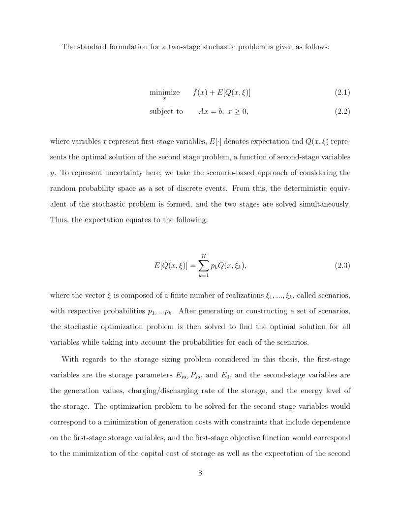
The standard formulation for a two-stage stochastic problem is given as follows:

minimizex

f(x) + E[Q(x, ξ)] (2.1)

subject to Ax = b, x ≥ 0, (2.2)

where variables x represent first-stage variables, E[·] denotes expectation and Q(x, ξ) repre-

sents the optimal solution of the second stage problem, a function of second-stage variables

y. To represent uncertainty here, we take the scenario-based approach of considering the

random probability space as a set of discrete events. From this, the deterministic equiv-

alent of the stochastic problem is formed, and the two stages are solved simultaneously.

Thus, the expectation equates to the following:

E[Q(x, ξ)] =

K∑

k=1

pkQ(x, ξk), (2.3)

where the vector ξ is composed of a finite number of realizations ξ1, ..., ξk, called scenarios,

with respective probabilities p1, ...pk. After generating or constructing a set of scenarios,

the stochastic optimization problem is then solved to find the optimal solution for all

variables while taking into account the probabilities for each of the scenarios.

With regards to the storage sizing problem considered in this thesis, the first-stage

variables are the storage parameters Ess, Pss, and E0, and the second-stage variables are

the generation values, charging/discharging rate of the storage, and the energy level of

the storage. The optimization problem to be solved for the second stage variables would

correspond to a minimization of generation costs with constraints that include dependence

on the first-stage storage variables, and the first-stage objective function would correspond

to the minimization of the capital cost of storage as well as the expectation of the second

8

stage solution. Including the initial state of charge of the storage as a first-stage variable

means that every considered scenario starts and ends the day with the same state of charge.

This is based on the assumption that the days are consecutive (i.e., the end of the first

scenario is linked to the beginning of the second scenario), and that each scenario cannot

start with an arbitrary E0 without having stored energy from the previous day to reach

that level. This two-stage concept as related to the storage sizing problem is illustrated

in Figure 2.1. Each scenario corresponds to a 24-hour period of wind and load, obtained

from historical datasets.

First Stage Variables

First Stage Variables

Second Stage Variables

s s s sN

E E PE E P

E P P P

ss ss

G in out

0

s

Scenarios

1 2 3 N-1

Figure 2.1: Two-stage stochastic optimization concept for the storage sizing problem

In Chapter 3, scenarios reduction is performed and two-stage stochastic optimization

is employed on a reduced set of scenarios, each weighted by a probability of occurrence.

The method to find these probabilities is also explained in this chapter. In Chapter 5, the

two-stage stochastic problem is combined with Model Predictive Control, discussed in the

following section.

2.2 Model Predictive Control

The look-ahead optimization procedure used in Chapters 5, 6, and 7 is called Model Pre-

dictive Control (MPC). MPC, also called receding horizon control, shown in Figure 2.2,

minimizes the cost of control decisions on a system over a prediction horizon N . This

9

is done by forming a model of the system to be controlled and optimizing over a chosen

number of time steps in the future using the predicted output of the system. After this

optimization from discrete times t to t + N is complete, only the actions for time t are

applied. Measurements from the actual system are then taken, the model is updated, and

the optimization is recalculated for the next time step [9].

Figure 2.2: Visual representation of Model Predictive Control.

The formulation for a discrete-time, nonlinear MPC problem is as follows [10]:

minimizex(t),u(t)

N∑

t=1

J(x(t), u(t)) (2.4)

subject to g(x(t), u(t)) = 0, t = 1...N, (2.5)

h(x(t), u(t)) ≤ 0, t = 1...N, (2.6)

x(t + 1) = f(x(t), u(t)), t = 0...N − 1, (2.7)

with state variables x and input variables u. Optimal values are calculated for the entire

horizon but only the first step is applied. The simulation moves to the next step and

the process is repeated using updated measurements of the system state. In this thesis,

examples of equality constraints (2.5) dependent only on the current timestep are the power

balance equations. An example of the inequality constraints (2.6) dependent on t would

10

be the generator output limits, limits on the state of charge of the storage device, and the

chance constraints, to name a few. Intertemporal constraints (2.7) could refer to generator

ramp limits and the energy balance equation for the storage, for example.

Model Predictive Control is used in Chapter 5 to determine the optimal size of the

storage by taking into account wind forecast errors which affect the energy in the storage.

Hence, a probability distribution for the energy in the storage around deterministic values

for each time step in the horizon which reflects the error in the predicted energy level.

These errors in the energy level prediction worsen depending on the point in time within

an optimization horizon. In Chapters 6 and 7, MPC is used to determine the optimal

actions for charging and discharging from energy storage.

2.3 Optimality Condition Decomposition and the Ap-

proximate Newton Directions method

In Chapter 6, the nonlinear AC optimal power flow MPC problem is decomposed into

subproblems. The distributed optimization methods developed in this thesis are based

upon Optimality Condition Decomposition (OCD) and the Approximate Newton Direc-

tions method (AND).

Optimality Condition Decomposition [11], a modified version of Lagrangian Relaxation

Decomposition, is used to decompose the considered optimization problem. Using this

decomposition method, separability is achieved by fixing certain coupled variables as con-

stants during each iteration step. The general optimization problem can be formulated as

11

follows:

minimizex1,...,xM

f(x1, . . . , xM)

subject to gq(xq) = 0, q ∈ 1, . . . ,M

hq(xq) ≤ 0, q ∈ 1, . . . ,M

gq,coup(x1, ..., xM) = 0, q ∈ 1, . . . ,M

hq,coup(x1, ..., xM) ≤ 0, q ∈ 1, . . . ,M

(2.8)

whereM is the total number of subproblems and xq are the decision variables in subproblem

q, where q ∈ 1, . . . ,M. Constraints gq and hq are constraints dependent only on vari-

ables xq in subproblem q. Constraints gq,coup and hq,coup are called “coupling constraints”

corresponding to constraints that contain variables from multiple subproblems.

Optimality Condition Decomposition decomposes this optimization problem by assign-

ing variables and constraints to specific subproblems. Every coupling constraint is assigned

to one specific subproblem which takes this constraint into account as a hard constraint

in its constraint set. This coupling constraint is taken into account as a soft constraint

in the objective function of the other subproblems. If a subproblem contains a constraint

with a variable belonging to another subproblem, that so-called “foreign” variable is set

to a constant value given by its corresponding subproblem. This value is updated at the

next iteration when the subproblems exchange these coupled variables. An optimization

problem is formed for each subproblem q ∈ 1 . . .M as follows:

12

minimizexq

fq = (f(x1, . . . , xq−1, xq, xq+1, . . . , xM)

+

M∑

n=1,n 6=q

λngn,coup(x1, ..., xq−1, xq, xq+1, ..., xM)

+M∑

n=1,n 6=q

µnhn,coup(x1, ..., xq−1, xq, xq+1, ..., xM))

subject to gq(xq) = 0,

hq(xq) ≤ 0,

gq,coup(x1, ..., xq, ..., xM) = 0,

hq,coup(x1, ..., xq, ..., xM)) ≤ 0.

(2.9)

Variables denoted with an overhead bar are foreign variables, set to constant values given

by their corresponding subproblem, and variables without the bar are the optimization

variables of that subproblem. λn and µn are the Lagrange multipliers for the equality

and inequality constraints (respectively) determined by the subproblem n for which this

constraint is a hard constraint. The Approximate Newton Directions method [4], which

can be applied to the decomposed problem, is used to solve the first-order optimality

conditions of the problem by considering the update for the subproblems separately. After

each subproblem has updated, the foreign variables are exchanged between subproblems.

This Newton-Raphson update is given as follows:

x(p+1) = x(p) + α ·∆x(p) = x(p) − α · (J (p)tot )

−1 · d(p), (2.10)

where p is the iteration counter. In the original problem (2.8), the right hand side vector d(p)

includes the first order optimality conditions for the optimization problem described above

in (2.8) ordered according to the subproblems and evaluated at x(p), and the update vector

13

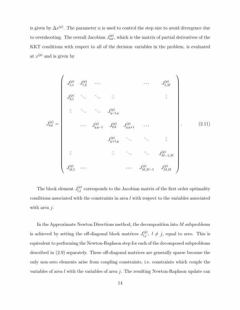
is given by ∆x(p). The parameter α is used to control the step size to avoid divergence due

to overshooting. The overall Jacobian J(p)tot , which is the matrix of partial derivatives of the

KKT conditions with respect to all of the decision variables in the problem, is evaluated

at x(p) and is given by

J(p)tot =

J(p)1,1 J

(p)1,2 · · · · · · J

(p)1,M

J(p)2,1

. . .. . .

......

.... . .

. . . J(p)q−1,q

· · · J(p)q,q−1 J

(p)q,q J

(p)q,q+1 · · ·

J(p)q+1,q

. . .. . .

...

......

. . .. . . J

(p)M−1,M

J(p)M,1 · · · · · · J

(p)M,M−1 J

(p)M,M

. (2.11)

The block element J(p)l,j corresponds to the Jacobian matrix of the first order optimality

conditions associated with the constraints in area l with respect to the variables associated

with area j.

In the Approximate Newton Directions method, the decomposition intoM subproblems

is achieved by setting the off-diagonal block matrices J(p)l,j , l 6= j, equal to zero. This is

equivalent to performing the Newton-Raphson step for each of the decomposed subproblems

described in (2.9) separately. These off-diagonal matrices are generally sparse because the

only non-zero elements arise from coupling constraints, i.e. constraints which couple the

variables of area l with the variables of area j. The resulting Newton-Raphson update can

14

then be solved in a distributed way, i.e.

x(p+1)q = x(p)

q + α ·∆x(p)q = x(p)

q − α · (J (p)q,q )

−1 · d(p)q , (2.12)

for q = 1, . . . ,M . Hence,

d(p) = [d(p)1 , . . . , d

(p)M ]T , (2.13)

x(p) = [x(p)1 , . . . , x

(p)M ]T (2.14)

∆x(p) = [∆x(p)1 , . . . ,∆x

(p)M ]T . (2.15)

In the considered problem, the optimization problem is decomposed according to geo-

graphical areas, i.e. the variables in x(p)q correspond to the variables associated with buses

in area q. As the considered problem spans multiple time steps, this variable vector includes

copies of all the variables within that area for all time steps in the optimization horizon,

i.e. PGi(0), . . . , PGi

(N − 1). The assignment of the coupling constraint in this application

is thus straightforward - because the coupling constraints correspond to the power balance

constraints at each border bus, the subproblem that is assigned the coupling constraint is

the one that corresponds to the area that contains that bus.

The advantage of this method is that instead of solving each subproblem to optimality

before exchanging information with the other subproblems, data can be exchanged after

each Newton-Raphson iteration. Additionally, unlike other Lagrangian-based decompo-

sition methods such as Lagrangian Relaxation and Augmented Lagrangian, there is no

need for a centralized entity or tuning of parameters to update the Lagrange multipliers;

subproblems simply exchange data directly with their neighbors and the updates for the

multipliers come directly from the other subproblems.

In Chapter 6, the optimization problem is first decomposed with OCD, and then modi-

fications of the AND method are derived and compared with convergence results using the

15

original AND method.

2.4 Unlimited Point Method

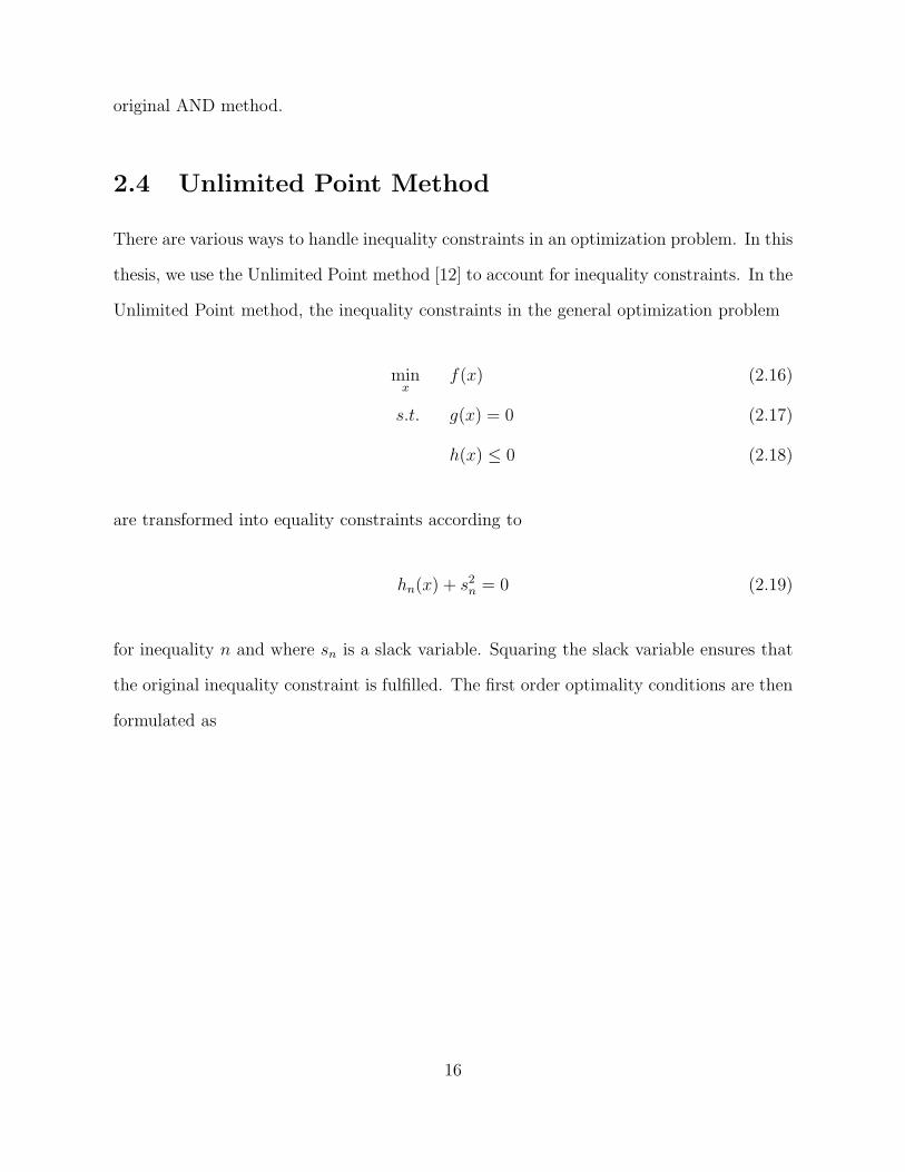
There are various ways to handle inequality constraints in an optimization problem. In this

thesis, we use the Unlimited Point method [12] to account for inequality constraints. In the

Unlimited Point method, the inequality constraints in the general optimization problem

minx

f(x) (2.16)

s.t. g(x) = 0 (2.17)

h(x) ≤ 0 (2.18)

are transformed into equality constraints according to

hn(x) + s2n = 0 (2.19)

for inequality n and where sn is a slack variable. Squaring the slack variable ensures that

the original inequality constraint is fulfilled. The first order optimality conditions are then

formulated as

16

∂f

∂x+ λT ·

∂g

∂x+ µ2T ·

∂h

∂x= 0 (2.20)

g(x) = 0 (2.21)

h(x) + s2 = 0 (2.22)

diag(µ) · s = 0 (2.23)

Hence, similar to the slack variables, the Lagrange Multipliers are also replaced with

squared variables to ensure that these Lagrange Multipliers take values which are greater

than zero without having to explicitly include such non-negativity constraints. In Chap-

ter 6, distributed optimization techniques are developed to solve the distributed AC OPF

problem. The Unlimited Point method is used to account for inequality constraints in

this chapter; however, the derivations of the distributed methods stay the same even if

another technique is used to incorporate inequality constraints into a Newton-Raphson

update (such as Interior Point).

17

Chapter 3

Optimal Storage Sizing and Scenario

Reduction

With the increasing penetration of renewable energy sources into the electric power grid,

a heightened amount of attention is being given to the topic of energy storage, a popular

solution to account for the variability of these sources. Energy storage systems (ESS)

can also be beneficial for load-levelling and peak-shaving, as well as reducing the ramping

of generators. However, the optimal energy and power ratings for these devices is not

immediately obvious. In this chapter, the energy capacity and power rating of the ESS is

optimized using two-stage stochastic optimization.

Depending on the application, certain storage technologies may be more appropri-

ate for certain purposes. The performance of each of these technologies differ by their

charge/discharge rate and maximum energy capacity. Storage technologies include, but

are not limited to: pumped hydro, compressed air, flywheels, double-layer or super/ultra

capacitors, and batteries (lead-acid, lithium-ion, sodium/sulfur) [13]. In this thesis, the

focus is on intra-hour generation dispatch to balance out fluctuations in the net load, i.e.,

demand minus wind generation, of the system. In the considered problem formulation, the

storage device is characterized by a maximum energy capacity, maximum power rating and

19

a roundtrip efficiency.

A range of literature can be found on the topic of optimal storage sizing for various

applications in power systems. In [14], tabu search is used to find the optimal size of an

energy storage system integrated with a thermal power plant. Random storage capacity

ratings are generated and then evaluated in a cost-benefit framework. The benefit of

storage is assumed to come solely from a peak-shifting application, and the charging and

discharging of the storage is determined by whether or not the forecasted load was higher

or lower than the average demand. Dynamic programming is used in [15] to determine

an optimal operating strategy for the storage and the optimal size of the storage is found

as a function of the reduction in the consumer’s electricity bill. Similarly to [14], a peak-

shifting application is chosen and the storage dis/charging decisions are rule-based. The

optimal size of the storage is then based on the optimal operating strategy of the storage.

Artificial neural network (ANN) control strategies are used to optimally control and size a

zinc-bromine battery in [16] for wind power applications. This paper showed that by using

ANN controllers, a lower cost storage is required. Rule-based decisions on charging and

discharging the battery solely for the purpose of accounting for the wind forecast error is

assumed. In this thesis, the dis/charging variables of the storage are continuous decision

variables in the optimization, and the system can benefit from the peak-shifting application

of the storage in addition to load-levelling and the balancing of fluctuations introduced by

renewable energy and demand. In Chapter 5, this formulation is extended further to utilize

storage to account for errors in wind forecasting.

In [17] and [18], stochastic optimization is used to optimize the size of an energy storage

system, with a focus on hourly dispatch using linear generation costs. In [17], scenarios are

generated using calculated probabilities based on wind and load correlations, where wind

forecasts are assumed to be known perfectly. In order to reduce the amount of considered

scenarios, fuzzy clustering is used in [18] to group scenarios together with similar net load

20

shapes and levels. In this thesis, the scenarios are comprised of the actual historical data of

wind and load, and scenarios are clustered based upon optimal storage sizes for individual

scenarios and the variance in system price for that scenario. By utilizing this relationship,

the problem size is reduced dramatically. There are many other papers on optimal storage

sizing under uncertainty and storage sizing using chance-constrained programming that

are discussed in Chapter 5 and are not covered here.

The objective in this section is to optimally size storage while minimizing generation

costs and maximizing the use of renewable energy fluctuations on an intra-hourly scale.

With this application, the benefit of storage not only comes from peak-shifting, but also

from reducing the ramping of generation. Wind is assumed to be must-take to maximize

the use of renewable energy in the system. We show that there is a relationship between

optimal storage size and variance in system price for this application, allowing scenarios

which are similar with respect to storage needs to be clustered together and represented

by a single scenario. Hence, the clustering operates on the similarities in optimal storage

size rather than on similarities on the inputs of the scenarios. A comparison between

this clustering technique and clustering based on similarities in net load is compared in

the simulation section. This reduced set of scenarios, each weighted with an appropriate

probability, is then taken into account in the two-stage stochastic optimization problem,

significantly reducing the overall problem size. Thus, two-stage stochastic optimization

becomes feasible even for a large number of considered scenarios [19].

21

3.1 Formulation of the Optimal Storage Sizing Prob-

lem

3.1.1 Storage Model

The model for the ESS used in this thesis is the following:

E(t+∆t) = E(t) + ηc∆tPin(t)−∆t

ηdPout(t), (3.1)

0 ≤ E(t +∆t) ≤ Ess, (3.2)

0 ≤ Pin(t) ≤ Pss, (3.3)

0 ≤ Pout(t) ≤ Pss, (3.4)

where E(t) is the energy level in the storage at time instant t. The model incorporates

separate variables for charging and discharging power, Pin and Pout, as well as separate

constants for the charging and discharging efficiencies, ηc and ηd. Variables Ess and Pss

correspond to the energy capacity and the power rating of the storage device. The constant

∆t is the time between control decisions. Since the focus in this thesis is on intra-hourly

economic dispatch, ∆t will be set to 10 minutes in the simulations.

3.1.2 Cost function and Constraints

In this section, the optimization problem formulation for both an individual scenario and

the overall two-stage stochastic problem is given.

Individual Scenario

Each scenario corresponds to a 24-hour period of net load, i.e., load minus wind generation.

It is assumed that the generators have quadratic cost curves defined by cost parameters

ai, bi, and ci, upper and lower limits PminGi and Pmax

Gi , and ramping limitations RGi. The

22

economic dispatch optimization problem to be solved for one scenario if storage size and

charging and discharging limits are given is as follows:

min

NT∑

t=1

(

NG∑

i=1

aiP2Gi(t) + biPGi(t) + ci

)

(3.5)

s.t. PminGi ≤ PGi(t) ≤ Pmax

Gi , (3.6)

|PGi(t+∆t)− PGi(t)| ≤ RGi, (3.7)

NG∑

i=1

PGi(t)− PL(t) + PW (t)

+ Pout(t)− Pin(t) = 0, (3.8)

0 ≤ Pout(t) ≤ Pss, (3.9)

0 ≤ Pin(t) ≤ Pss, (3.10)

0 ≤ E(t) ≤ Ess, (3.11)

E(NT ) = E0, (3.12)

E(t+∆t) = E(t) + ηc∆tPin(t)−∆t

ηdPout(t), (3.13)

with t = 1, ..., NT for all constraints and i = 1, ..., NG, where NT is the number of steps in

the optimization horizon and NG is the number of generators in the system. The generation

output for generator i at time step t is given by PGi(t), total wind generation by PW (t)

and total load by PL(t). The initial energy level in the storage device is set to E0. As

described in Section 2.1, Pss, Ess and E0 all become variables in the two-stage stochastic

optimization problem.

Two-Stage Problem

The overall problem formulation for the two-stage stochastic problem is given by:

23

min

NS∑

s=1

(

ws · TL ·NT∑

t=1

(

NG∑

i=1

aiP2Gi(s, t) + biPGi(s, t) + ci

))

+ dEss + ePss (3.14)

s.t. PminGi ≤ PGi(s, t) ≤ Pmax

Gi , (3.15)

|PGi(s, t+∆t)− PGi(s, t)| ≤ RGi, (3.16)

NG∑

i=1

PGi(s, t)− PL(s, t) + PW (s, t)

+ Pout(s, t)− Pin(s, t) = 0, (3.17)

0 ≤ Pout(s, t) ≤ Pss, (3.18)

0 ≤ Pin(s, t) ≤ Pss, (3.19)

0 ≤ E(s, t) ≤ Ess, (3.20)

E0 = E(s,NT ), (3.21)

E(s, t+∆t) = E(s, t) + ηc∆tPin(s, t)−∆t

ηdPout(s, t). (3.22)

Hence, constraints of this optimization problem are equivalent to those given in (5.15)-

(5.24), but now with distinct variables PGi, Pout, Pin, and E as well as values PL and PW

for each scenario s = 1...Ns. Variables Ess, Pss, and E0 are not dependent on t or s. These

variables are common to all scenarios; their optimal values are calculated while taking into

account all of the considered scenarios simultaneously. The constant values ws correspond

to the probability of occurrence of scenario s. The constants d and e correspond to the

cost parameters of the storage device with respect to the capacity and charging speed,

respectively, and TL is the expected lifetime of the storage in number of days.

It is advantageous to determine what factors directly impact the optimal solution for

the storage sizing problem, so individual scenarios which result in a similar optimal storage

size may be grouped together and a new representative scenario for that cluster is chosen

24

and weighted accordingly. It is obvious that the more scenarios that are considered in the

problem, the more accurate the frequency of certain cases of wind and load in the system

will be represented. Thus, it is desirable to utilize as many scenarios as possible. However,

the number of variables and constraints increases tremendously with increasing number of

scenarios rendering stochastic optimization computationally very intensive.

3.2 Relationship between Optimal Storage Size and

Variance in Locational Marginal Price

The price of electricity is determined by the marginal cost of generation, i.e. the cost

to generate one additional unit of power in the system. As the Lagrange Multiplier of

the power balance equation (5.13) corresponds to the sensitivity of the objective function,

in this case the overall generation cost, with respect to a change in this equation, i.e. a

change in load, the incremental cost is equal to the value of this Lagrange Multiplier. In

the following, we refer to this as the system price and denote it by λp.

Due to the fact that load and infeeds from renewable generation vary significantly

throughout the course of the day, the system price also varies over the day. The variance

of the system price, measured over the time period of one day, is defined as:

var(λp) =1

NT

NT∑

t=1

(λp(t)−mean(λp))2. (3.23)

For illustration purposes, we show the correlation between the system price variance

and the optimal storage size for a small system with three conventional generators and two

wind generators. First, the economic dispatch problem without storage is solved for a range

of different scenarios. This corresponds to optimizing for (5) and including constraints (6)

and (7) and the power balance equation (8) but without the charging/discharging from

the storage for each of these scenarios. The resulting variance in system price for each

25

of the scenarios is stored. Next, the optimization problem with storage as a variable,

i.e. (3.14)-(3.22) is solved for each scenario separately. Hence, only one single scenario

is taken into account in the optimization problem each time and the optimal storage size

and charging/discharging rate are determined as if this is the only occurring scenario. The

resulting variances in system price and the optimal storage sizes are plotted in Figure 3.1.

0 10 20 30 40 50 60 70 800

5

10

15

20

25

Var(λp) ($/MWh)2

Opt

imal

Sto

rage

Siz

e (M

Wh)

Figure 3.1: Relationship between marginal price and optimal storage size for system withthree conventional generators and two wind generators.

It is clear from the figure that the optimal capacity of the storage is positively correlated

with the variance in system price for that scenario. That is, the bigger the variance in price

over that scenario, the more beneficial it is to use storage. This can be attributed to a

great extent to the quadratic cost functions of the generators. Changes in the level of

generation and therefore ramping are implicitly penalized because of this quadratic cost.

Storage helps to alleviate the ramping of these generators, thus lowering the overall cost

of generation. In the presence of an increased penetration of intermittent sources such as

wind, the required ramping increases thereby increasing the value of storage. However, no

direct correlation was found between the optimal storage capacity and variance in wind or

load. The variance in system price was found to be the strongest indicator with respect to

optimal storage size for the considered problem formulation with quadratic cost functions.

This dependency has important implications on how to cluster scenarios. To show how

26

this is different from clustering scenarios based on similarities in net load, we show the

optimal storage sizes for five scenarios and their respective net load curves in Figures 3.2

and 3.3 for a system of 8 conventional generators and two wind generators.

0 10 20 30 40 50 60 70 800

2

4

6

8

10

12

14

Var(λp) ($/MWh)2

Opt

imal

Sto

rage

Cap

acity

(M

Wh)

s1s2s3s4s5

Figure 3.2: Optimal storage sizes for the 10 generator system and five different scenarios.

0 50 100 15012

13

14

15

16

17

18

19

Time (10−minute increments)

Net

Loa

d (p

.u.)

s1s2s3s4s5

Figure 3.3: Net load of five scenarios in the 10 generator system.

The two scenarios with the closest optimal capacity/variance in system price are sce-

narios 2 and 3. It is interesting to note that the net load for scenarios 2 and 3 have a very

large difference in magnitude. Scenario generation by methods which assume that scenar-

ios with similar net load values produce similar optimal storage capacities may therefore

not be an appropriate way to group scenarios in the considered problem formulation. Con-

27

sequently, we propose to use the correlation between system price and optimal storage size

as a means to cluster scenarios.

3.3 Hierarchical Clustering and Scenario Reduction

In [17], wind and load correlation probabilities are used for scenario generation. Scenarios

with similar net load shapes and levels are grouped together in [18], and fuzzy clustering

is used for scenario generation. In [20], uncertainties in wind and electricity prices are

taken into account and a sample average approximation method is used to reduce the

dimensionality of the scenarios.

As the number of scenarios considered in the optimization increases, the more accurately

the distribution of possible realizations of net load are represented. However, this also

increases the problem size to unmanageable levels, especially on a 10-minute dispatch

scale. Scenario reduction techniques have been employed for the energy storage sizing

problem, e.g. in [17] and [18]. However, as described earlier, these techniques focus on

load/wind correlations and net load analysis to determine similarity between scenarios.

Here, scenario reduction is performed by utilizing the discovered relationship between

the optimal storage capacity and variance in system price. We use a hierarchical centroid-

linkage clustering method [21] to form clusters of similar scenarios. In this clustering

technique, each scenario is first considered to be a separate cluster, and clusters are sub-

sequently combined into larger clusters until the desired number of clusters is obtained.

Hierarchical clustering is chosen over other conventional clustering methods because other

methods may group outlier clusters with other clusters instead of keeping them distinct,

which is desirable in our application. At each iteration of the process, centroids, which

correspond to the mean of all data points in their respective cluster, are calculated. The

centroid ci for cluster i is therefore defined as:

28

ci =1

Ni

∑

k∈Λi

xk, (3.24)

where Λi includes the set of points xi = [var(λp); Ess] included in cluster i and Ni is the

number of points in cluster i. Next, the Euclidean distances between all possible cluster

pairs (i, j) where i 6= j, are determined and compared. The pair that minimizes ‖ci − cj‖2

is combined into a new cluster m where the data points xm = xi ∪ xj. This process is

repeated until the desired number of clusters is achieved. Next, a representative scenario

is chosen for each cluster. This scenario xi, for each cluster i, is chosen to be the one that

is closest to the mean of that cluster; i.e.,

xi = argminxk∈Λi

‖xk − ci‖2 . (3.25)

For the considered application, each scenario corresponds to a specific realization of load

and wind generation for one day. Each of these scenarios results in one data point in the

correlation between storage size and variance in marginal cost. The clustering technique

is then used to cluster this two dimensional data into a pre-defined number of clusters.

As an example, 150 scenarios were run on the 8-generator, 2-wind plant system and

these scenarios were grouped into 10 clusters. In Figure 3.4, the result of the clustering is

shown. The number of scenarios in each cluster determines the probability of the resulting

representative scenario of that cluster, as shown in Figure 3.5. The data were normalized

by dividing by the maximum element in each direction so that the axes were equal before

performing the clustering.

The scattering is related to the fact that different sets of generators reach their limits for

different levels of net load, and therefore a different generator is setting the system price.

I.e., in one case with a large amount of wind, a coal plant that was usually producing

at capacity for most of the other scenarios was not at capacity. However, even with the

29

scattering multiple linear trends can be observed.

0 0.1 0.2 0.3 0.4 0.5 0.6 0.7 0.8 0.9 10

0.1

0.2

0.3

0.4

0.5

0.6

0.7

0.8

0.9

1O

ptim

al S

tora

ge S

ize

(Nor

mal

ized

MW

h)

Var(λp) (Normalized ($/MWh)2)

c1c2c3c4c5c6c7c8c9c10

Figure 3.4: Correlation and clustering for the 10 generator system, 150 scenarios and 10clusters.

0 0.1 0.2 0.3 0.4 0.5 0.6 0.7 0.8 0.9 10

0.1

0.2

0.3

0.4

0.5

0.6

0.7

0.8

0.9

1

Var(λp) (Normalized ($/MWh)2)

Opt

imal

Sto

rage

Siz

e (N

orm

aliz

ed M

Wh)

c8

c5

c7

c6

c3

c4

c2

c1

c9

c10

0.0133

0.0067 0.0067

0.5400

0.0200

0.0067

0.0133

0.0067

0.0067

0.3866

Figure 3.5: Representative clusters weighted by probabilities for the 10 generator system.

An overview over the proposed approach to determine the optimal sizing of the storage

device is given in Figure 3.6. First, the economic dispatch problem in (5.1) - (5.24) is

solved without any storage device in the system for every single scenario separately in

30

order to determine the variance in marginal generation cost before the deployment of

storage. Then, the problem in (3.14) - (3.22) is solved separately for each scenario with

storage as a variable, determining the optimal Ess, Pss, and E0 for that scenario. Next, the

scenarios are clustered into groups and representative scenarios are chosen for each cluster.

This reduced set of scenarios is used in the stochastic problem formulation (3.14) - (3.22)

to determine the overall optimal storage size.

Simulate all scenarios

separately with storage

variables included. Store

The optimal storage sizes

for each scenario.

Simulate all scenarios

separately without storage

in the system.

Store the resulting system

price for each scenario.

Form a 2D vector X that is

composed of the previous

two values and cluster the

values in X into groups.

Choose representative scenarios for

each cluster by choosing the scenario

closest to the centroid. Weight these

scenarios by the number of scenarios in

their represented cluster divided by the

total number of scenarios.

Perform two-stage stochastic optimization

using the new weighted representative

scenarios.

Figure 3.6: Flowchart of the overall algorithm.

31

Table 3.1: Generator parameters.

Generator a ($/MW/MWh) b ($/MWh) c ($/h) Capacity

Gas 0.76 15 370 250 MW

Coal 0.0079 18 772 330 MW

Nuclear 0.00059 5 240 350 MW

Gas 0.76 13 370 250 MW

Coal 0.0133 18 440 340 MW

Nuclear 0.00059 5.2 240 350 MW

Coal 0.014 18 772 330 MW

Coal 0.0078 17.7 440 330 MW

3.4 Simulation Results

Here, we first give an overview over the simulation setup and then discuss the simulation

results.

3.4.1 Simulation Setup

Simulations were performed on a power system with eight conventional generators and

two wind power plants. The 10-minute demand data for 150 days was taken from ISO

New England [22] and the data for the wind outputs was taken from the Eastern Wind

Integration Transmission Study (EWITS) [23]. Results are given for various levels of wind

energy penetration. The chosen cost function data and capacities for the generators are

given in Table 3.1. The storage technology used in these simulations has a roundtrip

efficiency of 95% and capital costs of the energy capacity and power converter size as

$1, 666/kW ·10−min and $500/kW , respectively. The storage is assumed to be operating

without degradation for the assumed time period TL and generation costs are minimized

over a period of 20 years; i.e., TL = 20 · 365.

32

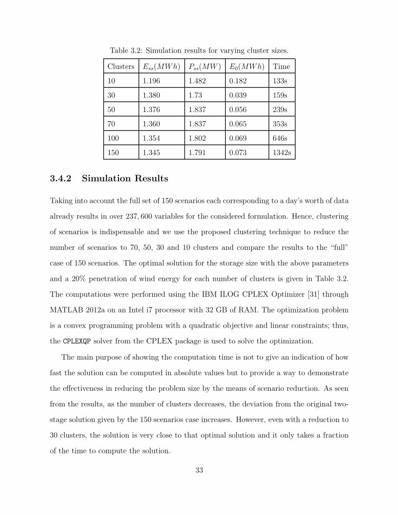
Table 3.2: Simulation results for varying cluster sizes.

Clusters Ess(MWh) Pss(MW ) E0(MWh) Time

10 1.196 1.482 0.182 133s

30 1.380 1.73 0.039 159s

50 1.376 1.837 0.056 239s

70 1.360 1.837 0.065 353s

100 1.354 1.802 0.069 646s

150 1.345 1.791 0.073 1342s

3.4.2 Simulation Results

Taking into account the full set of 150 scenarios each corresponding to a day’s worth of data

already results in over 237, 600 variables for the considered formulation. Hence, clustering

of scenarios is indispensable and we use the proposed clustering technique to reduce the

number of scenarios to 70, 50, 30 and 10 clusters and compare the results to the “full”

case of 150 scenarios. The optimal solution for the storage size with the above parameters

and a 20% penetration of wind energy for each number of clusters is given in Table 3.2.

The computations were performed using the IBM ILOG CPLEX Optimizer [31] through

MATLAB 2012a on an Intel i7 processor with 32 GB of RAM. The optimization problem

is a convex programming problem with a quadratic objective and linear constraints; thus,

the CPLEXQP solver from the CPLEX package is used to solve the optimization.

The main purpose of showing the computation time is not to give an indication of how

fast the solution can be computed in absolute values but to provide a way to demonstrate

the effectiveness in reducing the problem size by the means of scenario reduction. As seen

from the results, as the number of clusters decreases, the deviation from the original two-

stage solution given by the 150 scenarios case increases. However, even with a reduction to

30 clusters, the solution is very close to that optimal solution and it only takes a fraction

of the time to compute the solution.

33

The value of using stochastic optimization can be analyzed in comparison with other

methods. In Table 3.3, the stochastic solutions for the battery energy capacity using

various numbers of clusters are compared first with the method of clustering based upon

net load, and secondly with using a simple weighted average of representative scenarios.

In the third column of the table, results are tabulated for the case when the represen-

tative scenarios are formed by clustering based on vectors of net load for each scenario s,

i.e., xs = PL(s, t) − PW (s, t). The “weighted average” of clusters as shown in the fourth

column of the table refers to the average of optimal Ess sizes from the representative sce-

narios weighted by their probability as calculated from scenario reduction. In the case of

150 scenarios, the “weighted average” does not include representative scenarios, but rather

refers to the average of the optimal solution of the original 150 scenarios, each with equal

probability.

It can be seen that performing stochastic optimization in both cases, comparing with

the weighted average approach, results in a storage size which is significantly closer to

the solution of the overall stochastic optimization. With the averaging approach, outlier

scenarios (in this case, with a larger battery size) are given a higher weight and influence

the optimal solution such that the overall capacity is increased. By clustering based on

var(λp), more information is gained by increasing the number of clusters, reducing the

distance from the original solution as more clusters are added. The solutions obtained by

clustering based on net load are relatively arbitrary and do not seem to cluster together

the scenarios which result in similar optimal storage sizes.

The optimal amount of storage in the system can be analyzed for various levels of

wind penetration. In Figure 3.7, the optimal amount of storage capacity for 100 scenarios

is shown for varying levels of wind penetration. Here, wind energy penetration level is

defined as the percentage of demand in terms of energy that is supplied by wind energy on

average over all considered scenarios. Table 3.4 lists the results of stochastic optimization

34

Table 3.3: Optimal Ess (MWh) size using various cluster sizes and techniques.

Clusters Clustering based onvar(λp)

Clustering based onnet load

Weighted Average

10 1.196 1.326 1.837

30 1.380 1.351 1.645

50 1.376 1.260 1.597

70 1.360 1.149 1.654

100 1.354 1.010 1.634

150 1.345 1.345 2.225

with increasing number of clusters for 0%, 10%, and 20% of wind energy penetration. As

seen from the figure and table, the optimal amount of storage increases with the level of

penetration. This can be attributed to the fact that a higher penetration of wind results in

more variation in the net load, making it more beneficial to deploy a larger storage device.

Table 3.4: Optimal Ess size in MW · 10−mins for different levels of wind penetration.

Clusters 0% Wind 10% Wind 20% Wind

10 3.285 4.675 7.818

30 3.049 4.650 7.942

50 3.103 4.656 7.612

70 3.068 4.635 7.287

100 3.054 4.636 7.546

35

0 20 40 60 80 100 120 140 160 180 2000

10

20

30

Var(λp) ($/MWh)2

20% Wind Energy Penetration

0 10 20 30 40 50 60 70 800

5

10

15

20

Opt

imal

Sto

rage

Cap

acity

(M

W⋅ 1

0−m

inut

es)


0 10 20 30 40 50 60 70 800

5


Figure 3.7: Optimal storage capacity for various levels of wind penetration.

36

Chapter 4

Optimal Storage Placement

With a heightened availability of renewable energy in the power grid comes a corresponding

need for an increase in transmission capacity. If this increase is not provided, line conges-

tions and an increase in generation cost become imminent. The optimal placement and

usage of storage devices is one way to avoid congestions and the increase in cost. While

not as prevalent in the current literature as the optimal storage sizing problem, the prob-

lem of optimal storage siting has been addressed from various perspectives [24]-[27]. In

[24], the optimal location and capacity for a battery energy storage system in a residential

distribution system with a high penetration of photovoltaic generation is determined. The

optimal placement of the device was considered on a case-by-case basis for three different

placements for a particular given day of the year. Consideration of the optimal placement

problem on a case-by-case basis, or when considering scenarios separately and not simulta-

neously in the optimization problem, is a large simplification of the problem and can result

in suboptimal placement of the storage as well as operation of the storage.

The work in [25] uses genetic algorithms and probabilistic optimal power flow to de-

termine the optimal locations of storage within a deregulated power system with wind

generation. A DC OPF framework is used, and the optimal capacity of the storage is

determined after the optimization for the location is complete, i.e., the state of charge is a

37

function of generation and load and not separate dis/charging decision variables. The aim

of energy storage in this paper is to store the wind energy which would otherwise be cur-

tailed and utilize it during the peak hours. However, having this model for the operation

energy storage neglects the additional benefits gained from utilizing energy storage to bal-

ance fluctuations in the power supply and reduce the amount of generator ramping, which

can reduce the overall generation cost in the system, and can also result in suboptimal

dis/charging decisions on the storage.

Results in [26] concluded that the optimal location of storage is not strongly affected

by the amount of wind penetration or location of wind in the system, but rather that line

congestions had a large influence on the optimal location. This conclusion was confirmed

by the results presented in this chapter as well. However, in this work, the demand and

generation profiles are assumed to be cyclic, the timescale is half-hourly, and the overall

storage capacity in the system is fixed. Active and reactive power flows are considered,

but the simplifying assumption is made that reactive power is a fixed percentage of the

active power. Without simultaneously considering a range of possible days (or providing a

method to choose which days could represent a diverse range of states of the power system),

the resulting storage placement may be well suited to a particular scenario but not a wide

range of scenarios.

Both transmission expansion and placement for storage are considered in [27] in the

form of a mixed-integer programming problem on a 6-bus test system. A fixed capacity of

the storage is assumed, and operations are considered on the hourly timescale. A single

day is used to represent each of the four seasons of a year, and the planning horizon is

considered over an eight year period. In order to make the problem less computationally

intense, the assumption is made that the expansions will take place only in the areas of

the grid affected by congestion; however, this neglects the benefits gained from utilizing

storage to balance fluctuations in other areas of the grid. This paper aims to answer the

38

question of transmission expansion and placement of storage simultaneously, but does not

find the optimal size of the storage in the optimization, which can affect the outcome of

the considered problem.

In this thesis, a similar optimization problem to the two in the previous two sections is

formulated as a two-stage stochastic optimization problem minimizing generation costs of

all generators in the system as well as the capital cost of a storage device in the WSCC 9-bus

test system. A 10-minute dispatch scale is assumed, so that the storage can also provide

a balance to intra-hourly fluctuations introduced by wind. The size of the storage affects

the placement and the operation of the storage, so these two objectives are considered

simultaneously. The resulting two-stage stochastic optimization problem then minimizes

the cost of storage and the cost of generation in a DC OPF framework with line limits

over a number of scenarios. The first stage decisions correspond to the optimal number of

storage devices, as well as their optimal locations and maximum capacities. The maximum

number of storage devices can be fixed if it is known how many storage devices are to be

placed. A scenario reduction technique is used to cluster similar days together which are

then used as the scenarios in the two-stage stochastic optimization problem.

4.1 Formulation of the Optimal Storage Placement

Problem

The two-stage stochastic optimization problem is formulated as a mixed-integer DC optimal

power flow problem. The cost function and constraints are described below.

39

4.1.1 Cost Function

The cost function is given by

min

NS∑

s=1

(

ws · TL ·NT∑

t=1

(

NG∑

i=1

aiP2Gi(s, t) + biPGi

(s, t) + ci

))

+

NB∑

i=1

(dEssi + ePssi + Cc · binEi) (4.1)

First stage binary variables binEi denote if there is a storage device at bus i (1) or not

(0) with associated one-time installation/construction costs Cc. Variables Essi and Pssi

describe the energy capacity and power converter rating of a storage device at bus i, with

associated capital costs d and e, respectively. These variables are forced to zero in the

constraints if the corresponding binEi at that bus is zero.

Generation costs PGi(s, t), corresponding to the active power generation at bus i, are

minimized over all scenarios. Here, we again use entire days as the scenarios and the

resolution for the time steps t is 10 minutes. Constant values ai, bi, and ci are the cost

parameters for the active power generator at bus i. Values ws describe the probability of

occurrence of scenario s. The expected lifetime that the storage will be fully functioning

is TL, given in number of scenarios (days). Integers NS, NT , NG, and NB are the number

of scenarios, time instances in one scenario, and number of buses, respectively.

4.1.2 Constraints

The optimization problem to be solved includes the objective function in (4.1) subject to:

PGi≤ PGi

(s, t) ≤ PGi, (4.2)

|PGi(s, t+∆t)− PGi

(s, t)| ≤ RGi, (4.3)

NG∑

i=1

PGi(s, t)− PLi

(s, t) + Pfi(s, t)

40

+ Pouti(s, t)− Pini(s, t) = 0, (4.4)

Pij ≤ Pij(s, t) ≤ Pij, (4.5)

0 ≤ Pouti(s, t) ≤ Pssi, (4.6)

0 ≤ Pini(s, t) ≤ Pssi , (4.7)

0 ≤ Ei(s, t) ≤ Essi, (4.8)

0 ≤ Essi ≤ 10000 · binEi, (4.9)

0 ≤ Pssi ≤ 10000 · binEi, (4.10)

NB∑

i=1

binEi ≤ binEmax, (4.11)

E0 = Ei(s,NT ), (4.12)

Ei(s, t+∆t) = Ei(s, t) + ηc∆tPini(s, t)−

∆t

ηdPouti(s, t). (4.13)

for i = 1...NB, s = 1...NS, t = 1...NT , and where the variables are defined as in section

4.1.1 and the remaining variables defined as follows:

Pfi forecasted active power output of wind generator at bus i

PLiactive power load at bus i

Pinipower injected into storage at bus i

Pouti power drawn from storage at bus i

Pij active power flowing on line ij

Ωi set of buses connected to bus i

Ei energy level in storage at bus i

ηci charging efficiency of storage at bus i

ηdi discharging efficiency of storage at bus i

PGimaximum active power output of generator at bus i

41

P ij maximum power flow on line ij

bineEmax maximum number of storage devices in the system

Optional constraints include fixing an individual binEi to 0 or 1 if it is known a priori that

a storage device is either desired or undesirable at a particular bus. The value 10, 000 was

chosen in constraints (4.9) and (4.10) to be about 50 times the maximum value of Ess that

was observed in simulations.

4.2 Storage Size/LMP Relationship

When the grid of the power system is taken into account, there no longer exists only a

single power balance equation in the constraint set. The power must be balanced at each

bus, and when congestion is present in the system, the Lagrange multipliers corresponding

to these power balance equations are not equal [28]. We call each Lagrange multiplier

corresponding to the power balance equation at each bus the locational marginal price

(LMP), or shadow price, at that bus [30]. In a similar analysis to what was performed

in Chapter 3 with an observation of the relationship between the marginal price and the

optimal storage size, here, an observation is made between the optimal storage size at

each bus and the locational marginal price at that bus (without storage). The results here

assumed a storage device with ηc ·ηd = 85%, d = $600/kWh, and e = $400/kW ; i.e., a large

lithium ion battery [13]. The one-time installation cost for the storage was assumed to be

Cc = $2000. The line parameters and generator cost parameters for the 9-bus system are

found in the Appendix. The computations shown in this chapter were performed using the

IBM ILOG CPLEX Optimizer [31] through MATLAB 2013b on an Intel Xeon processor

with 128 GB of RAM.

Simulations were run on the WSCC 9-Bus test system [29]. The modified 9-bus test

system, seen in Figure 4.1, contains three conventional generators, one wind power plant,

42

six lines, and three loads.

2

1

3

w

72

8

9 3

1

4

5 6

Figure 4.1: WSCC 9-Bus test system

4.2.1 Optimal siting without congestion

Without any congestion in the system, the location of the storage in the system has little

impact. Storage can still provide to be useful for balancing fluctuations in the power

supply and for peak-shifting, and the correlation between the optimal storage size and LMP

exists, as shown in Figure 4.2 for the optimal placement of one storage device. However,

multiple locations could result in a very similar objective function value, not really making

it advantageous to place the storage at one bus versus another. For example, the simulation

results in Figure 4.2 indicate that, for most scenarios, bus 9 is the optimal location for the

battery. But because in this case the problem does not have a unique solution, it is a fairly

arbitrary result without any congestion and by using a DC power flow approximation, only

the size matters as opposed to the location.

43

0 5 10 150

5

10

Bus 1

0 5 10 150

5

10

Bus 2

0 5 10 150

5

10

Bus 3

0 5 10 150

5

10

Bus 4

Opt

imal

Sto

rage

Siz

e (M

Wh)

0 5 10 150

5

10

Bus 5

0 5 10 150

5

10

Bus 6

0 5 10 150

5

10

Bus 7

0 5 10 150

5

10

Bus 8

Var(λi) ($/MWh)2

0 5 10 150

5

10

Bus 9

Figure 4.2: Optimization of 20 individual scenarios showing correlation of optimal storagesize at each bus with variance in LMP with no congestion

4.2.2 LMP/Storage size relationship with congestion

Optimal siting of the storage is much more valuable when congestion exists in the system.

To demonstrate the effect of different LMPs on the optimal storage size at each bus, thermal

limits on the lines are put into place. In the first example, a single line limit is placed on

line 2, the line connecting buses 4 and 6, as seen in Figure 4.3. The limit is set to 9 MW

so that congestion exists during the peak hours of almost every scenario. An unlimited

number of storage devices is considered in the system; i.e., binEmax = NB.

44

2

1

3

w

72

8

9 3

1

4

5 6

Figure 4.3: 9-Bus test system with line congestion

0 5 10 150

2

4Bus 1

0 5 10 150

2

4Bus 2

0 5 10 150

2

4Bus 3

0 5 10 150

2

4Bus 4

Opt

imal

Sto

rage

Cap

acity

(M

Wh)

0 5 10 150

2

4Bus 5

0 5 10 150

2

4Bus 6

0 5 10 150

2

4Bus 7

0 5 10 150

2

4Bus 8

Var(λi) ($/MWh)2

0 5 10 150

2

4Bus 9

Figure 4.4: Optimization of 20 individual scenarios showing correlation of optimal storagesize at each bus with variance in LMP with congestion

The results for 20 scenarios with line 2 congested are given in the plots in Figure 4.4.

As observed from the figure, it is most advantageous to place the storage device at bus 6.

45

Cheap generation from generator 1 can charge the storage during off-peak hours, and the

load can consume the stored energy during peak hours when the line between buses 4 and

6 is congested. One such scenario is shown in Figure 4.5. When a storage device is placed

at bus 6, is used to supply the load at bus 6 during the peak hours of the day, as well as

balance fluctuations introduced by wind.

0 50 100 1500

5

10

15

20

Time

MW

Load at bus 6Power into storageat bus 6Power out ofstorage at bus 6

Figure 4.5: A single scenario showing the storage usage at bus 6

Using this relationship between optimal storage size and variance in locational marginal

price, a similar scenario reduction technique as derived in the previous chapter can be

performed to reduce the size of the scenario set. Hierarchical centroid-linkage can be used

to cluster the data; however, in higher dimensions than before. Now, instead of clustering

in two-dimensions with the variance in system price and one optimal storage size, we have

multiple locational marginal prices and optimal storage sizes. As with the storage sizing

problem, the centroid cd for cluster d is defined as:

cd =1

Nd

∑

k∈Λd

xk, (4.14)

where Λd includes the set of points xd = [var(λ1), Ess1 ; ...var(λNB), EssNB

] in cluster d,

46

for all buses i = 1...NB for which binEi is nonzero. Variable Nd is the number of points

in cluster d. Next, the Euclidean distances between all possible cluster pairs (d, c) where

d 6= c, are determined and compared. The pair that minimizes ‖cd − cc‖2 is combined into

a new cluster m where the data points xm = xd ∪ xc. This process is repeated until the

desired number of clusters is achieved. Next, a representative scenario is chosen for each

cluster. This scenario xd, for each cluster d, is chosen to be the one that is closest to the

mean of that cluster; i.e.,

xd = argminxk∈Λd

‖xk − cd‖2 . (4.15)

As in the previous chapter, each scenario corresponds to a specific realization of load

and wind generation for one day. Each of these scenarios results in one data point in the

correlation between storage size and variance in marginal cost over all considered buses.

The clustering technique is then used to cluster the multi-dimensional data into a pre-

defined number of clusters.


In this section, various cases are considered for the storage siting problem. The number of

considered storage devices is varied, as well as the number of congested lines.

4.3.1 Solution of the Placement Problem

The optimization problem solved in this chapter is a convex mixed-integer quadratic prob-

lem. In the following simulations, it is confirmed by CPLEX’s branch-and-bound MIQP

solver that the output is the optimal integer solution. Due to the efficient implementation

of the dual QP simplex algorithm for MIQPs in CPLEX, other algorithms for solving MIQP

problems are not used or implemented in CPLEX for problems of this type [32] (however,

47

the Outer Approximation algorithm is used for CPLEX’s MIQCP (mixed-integer quadrat-

ically constrained problem) solver). The optimization can be performed faster if a larger

tolerance is specified, but because time is not as much of an issue in the planning problem,

1 · 10−9 was used for the tolerance to ensure that the solution is optimal.

4.3.2 Case 1: One Congestion

In the first example, the limit on the line connecting buses 4 and 6 is set to 10 MW. From

the results in section 4.2.2, we can see that when congestion is present on this line, the

system can benefit from placing storage at bus 6. Here, in the first considered case, the

two-stage optimization is performed over 20 scenarios to determine the optimal number

and sizes of storage devices. Next, we reduce the set of 20 scenarios to a set of 10 scenarios

and subsequently a set of 5 scenarios and perform two-stage optimization.

Table 4.1: Optimal solution from 20 scenarios.

Location Essi (MWh) Pssi (MW)

Bus 1 21.896 3.756

Bus 4 3.392 0.569

Bus 6 27.874 5.702

Table 4.2: Optimal solution from 20 scenarios clustered into 10.


Bus 1 17.704 3.048

Bus 4 5.9528 0.891

Bus 6 28.576 5.813

In both the original case with 20 scenarios and the reduced set of 5, as seen in Tables

4.1, 4.4, and 4.3, the results of the optimization indicate that it is optimal to place three

storage devices in the system, at buses 1, 4, and 6. The optimal storage size at bus 6

48

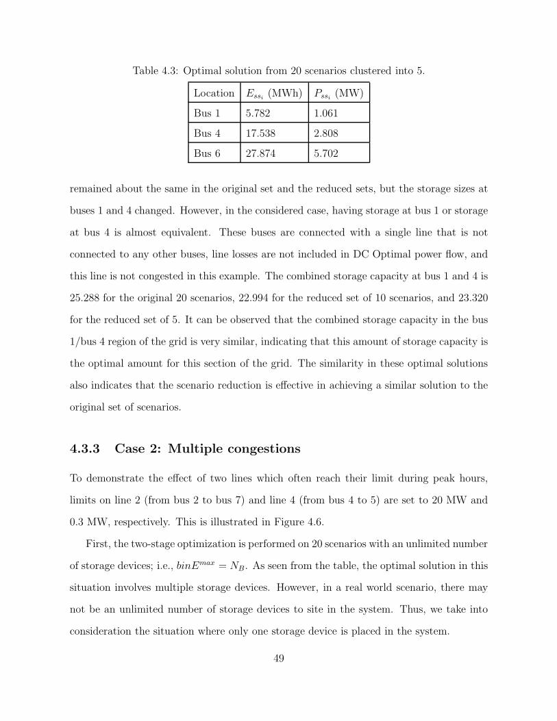
Table 4.3: Optimal solution from 20 scenarios clustered into 5.


Bus 1 5.782 1.061

Bus 4 17.538 2.808

Bus 6 27.874 5.702

remained about the same in the original set and the reduced sets, but the storage sizes at

buses 1 and 4 changed. However, in the considered case, having storage at bus 1 or storage

at bus 4 is almost equivalent. These buses are connected with a single line that is not

connected to any other buses, line losses are not included in DC Optimal power flow, and

this line is not congested in this example. The combined storage capacity at bus 1 and 4 is

25.288 for the original 20 scenarios, 22.994 for the reduced set of 10 scenarios, and 23.320

for the reduced set of 5. It can be observed that the combined storage capacity in the bus

1/bus 4 region of the grid is very similar, indicating that this amount of storage capacity is

the optimal amount for this section of the grid. The similarity in these optimal solutions

also indicates that the scenario reduction is effective in achieving a similar solution to the

original set of scenarios.

4.3.3 Case 2: Multiple congestions

To demonstrate the effect of two lines which often reach their limit during peak hours,

limits on line 2 (from bus 2 to bus 7) and line 4 (from bus 4 to 5) are set to 20 MW and

0.3 MW, respectively. This is illustrated in Figure 4.6.

First, the two-stage optimization is performed on 20 scenarios with an unlimited number

of storage devices; i.e., binEmax = NB. As seen from the table, the optimal solution in this

situation involves multiple storage devices. However, in a real world scenario, there may

not be an unlimited number of storage devices to site in the system. Thus, we take into

consideration the situation where only one storage device is placed in the system.

49

2

1

3

w

72

8

9 3

1

4

5 6

Figure 4.6: 9-Bus test system with two line congestions

Table 4.4: Optimal solution from 20 scenarios with two congested lines.


Bus 1 10.672 1.777

Bus 3 1.366 0.4198

Bus 4 14.947 2.637

Bus 5 42.487 7.181

Bus 6 1.436 0.390

Bus 8 0.720 0.197

Bus 9 3.083 0.711

Table 4.5: Optimal solution from 20 scenarios with two congested lines and one battery.


Bus 7 49.957 8.587

As can be seen from Table 4.5, the optimal location for one storage device in the system

with two congestions is at bus 7. During the times when the lines are congested, cheaper

generation from buses 1 and 2 can be supplied from a storage device that has been charged

50

in the off-peak hours at bus 7. The results in these two tables are interesting because the

optimal solution with unlimited storage devices does not place storage at bus 7, but when

running the optimization to site one storage device, bus 7 is the one that is chosen. This

could be due to two factors. In the first case with unlimited storage, storage is not only

placed for the purpose of alleviating line congestions, but also for peak-shifting and load

levelling. The storage placed at buses 1, 4, and 6 could serve this purpose, for example. The

storage devices placed at buses 5 and 8, the areas more affected by congestion, can charge

during times of no congestion serve the load at these buses during times of congestion. In

the one storage case, a storage device placed at bus 7 can serve a similar purpose to these

two loads.

The results of the storage siting problem indicate that the optimal location of the stor-

age is highly dependent on line congestions. By the use of optimally placed storage, energy

can be stored in the storage during off-peak hours and utilized during times when line con-

gestions may occur, reducing the costs incurred by the congestions. Without congestion

in the system, the specific location of the storage is less useful than optimally sizing the

storage. In future work, by either performing AC OPF instead or by including a model for

the line losses, the optimal solution will take into account that depending on the location

of the device, power losses can be minimized in the case with no congestions.

51

Chapter 5

Chance Constraints for Wind

Forecast Errors

Chapter 3 focused on finding the optimal capacity of a storage device under the assumption

that the wind forecast was known with certainty. However, this will assumption will rarely

be the case, and errors in wind forecasts can have a significant impact on the benefit gained

from energy storage. In this chapter, we focus on the intra-hour generation dispatch to

balance not only the intermittency of the wind generation, but also the uncertainty in

the wind forecast. Sizing a storage device for various purposes while taking into account

uncertainty in the optimization problem has been proposed in the literature. In [34],

persistence scenarios are employed, with the conclusion that such a technique can prove

to be useful for power capacity sizing but not as much for energy capacity sizing. The

assumption is made that the power and energy capacities are optimized independently.

Here, the power and energy capacity of the storage device, as well as the cost of generation,

are optimized simultaneously. In [35], the optimal sizing problem was considered from

an electricity market perspective, serving as a hedge against wind uncertainties. In the

combined wind/storage power plant framework, it is assumed that the wind power plant

operator will want to minimize the deviations from his contract and when excess power is

53

produced, the storage will be charged, and when more power is needed, the storage will

discharge. In this thesis, rather than penalize deviations from a wind power producer’s

contract, we are concerned with the system point of view where we wish to maximize the

use of wind and minimize the generation costs, with the goal of increasing the overall social

benefit of the system.

Both stochastic wind and demand are assumed in [36], and Monte-Carlo sampling of

the distributions, which are assumed to be Gaussian with zero mean and equal variance

at each timestep, is used to determine the optimal storage size. Certain reliability indices

are also taken into account in the optimization. The load profile used for the week-long

optimization period consists of a single day of historical data that is repeated and scaled.

In this thesis, we use purely historical data for both the wind and the load profiles, and no

assumptions are made about the patterns of these profiles. While the distribution of the

forecast errors at each time step in the horizon are assumed to be the same, the aggregation

of these errors is taken into account by adjusting the distribution of the energy level at

each time step.

Chance, or probabilistic, constrained programming has been utilized in many areas of

power system optimization. Particularly, to take into account wind uncertainty in the

energy storage sizing problem, chance constraints are used in [37], however, Monte-Carlo

sampling is used to generate scenarios; i.e., there is no analytical formulation for the con-

sideration of uncertainty. The stochastic unit commitment problem is addressed using

chance constraints in [38] by breaking up the original stochastic problem using a multi-

variate probability constraint into a sequence of easier to solve stochastic problems each of

which can be reduced to a deterministic problem. The approach eventually converges to

the solution of the stochastic problem. In [39], a Monte-Carlo approach is taken to solve

a different problem, namely the chance constrained AC OPF problem. On a 10-minute

dispatch scale as considered in this thesis, performing many Monte-Carlo simulations may

54

result in a time consuming optimization problem. Deriving an analytical form of the chance

constraint only requires a single optimization problem to be solved. Analytical forms of

the chance constrained security constrained OPF are derived in [40] and [41] where the

probabilistic constraints are formulated with respect to line flow limits. The assumptions

made in these papers, as in this thesis, is that the wind forecast error can be modeled

as a Gaussian distribution. The benefits of this are discussed in more detail later in this

chapter as well as in [40].

Here, chance constraints are formed for the minimum and maximum state of charge

of the storage device. The power and energy capacity of the storage device are optimized

simultaneously. The advantage of the method presented in this thesis is that no approx-

imate techniques such as Monte-Carlo simulations are used; rather, an analytical form

of the probabilistic constraints is derived and the optimization is solved directly. Also,

the control actions are considered on a 10-minute scale rather than on an hourly time

scale, allowing for storage to balance out intra-hourly fluctuations and uncertainties due

to wind. Furthermore, we assume that the storage is operated using a model predictive

control scheme, i.e. with a receding horizon, as opposed to a single multi-step optimization

problem for the time frame of a scenario as is usually done in the previous literature. By

considering aggregated probability distribution functions for the time steps in the opti-

mization horizon, we also account for the fact that prediction errors at the beginning of

the optimization horizon influence the operation of the storage at later steps, which is very

important when sizing the storage.

5.1 Modeling and Operation

The same storage model as described in Chapter 3 in equations (3.1)-(3.4) is used here.

The variable ∆t, the time between control decisions and the time between when wind

forecasts are given, is set to 10 minutes in our simulations for the purpose on focusing on

55

intra-hourly economic dispatch.

5.1.1 Predictive Optimization

It is assumed that the storage, once placed in the system, is operated using a model

predictive control approach. That is, the generation and storage outputs are determined

by optimizing over H time steps to minimize the overall supply cost, then the output

corresponding to the first step in the horizon is applied, and the optimization is carried

out again over a shifted time horizon of H time steps [9]. This concept is described

in more detail in Chapter 2. Hence, here we formulate the deterministic multi-timestep

optimization problem which will be incorporated into the storage sizing problem in the

next section.

The generators are modeled using quadratic cost functions defined by cost parameters

ai, bi, and ci, minimum and maximum generation limits PminGi and Pmax

Gi , and ramping

limitations RGi. The resulting cost function for the problem is given by

minPGi

H−1∑

h=0

NG∑

i=1

(

aiP2Gi(h) + biPGi(h) + ci

)

, (5.1)

subject to the following constraints 1:

s.t. PminGi ≤ PGi(h) ≤ Pmax

Gi , (5.2)

|PGi(h+ 1)− PGi(h)| ≤ RGi, (5.3)

NG∑

i=1

PGi(h)− PL(h) + PW (h)

+ Pout(h)− Pin(h) = 0, (5.4)

1As we only consider operation here, the storage size and maximum charging rate is fixed in thisformulation.

56

0 ≤ Pout(h) ≤ Pss, (5.5)

0 ≤ Pin(h) ≤ Pss, (5.6)

0 ≤ E(h + 1) ≤ Ess, (5.7)

E(H) = E0, (5.8)

E(h+ 1) = E(h) + ηc∆tPin(h)−∆t

ηdPout(h), (5.9)

for h = 0...H − 1, and i = 1, ..., NG, where NG is the number of generators in the system

and it is assumed that the time between to time steps in the optimization horizon is ∆t.

The generation output for generator i at time step h within the horizon is denoted by

PGi(h), the total wind generation by PW (h), and the total load by PL(h). The initial

energy level in the storage device, E(0), is set to E0. Both load and wind generation are

predicted values.

5.1.2 Forecast Error Modeling

In order to incorporate uncertainty into the problem formulation, a model of the typical

forecast error is needed. As we will focus on wind generation as the non-dispatchable

resource, we use three months of wind forecast and actual wind data from the Bonneville

Power Administration [42] to analyze forecast errors in wind predictions. A histogram of

the percent deviation between the actual and forecasted wind is shown in Figure 5.1. A

normal distribution with mean µp and variance σ2p is fitted to this data, as proposed in

[36], [41]. The high kurtosis of the data set may indicate that a distribution other than

Normal may be more accurate; however, the use of the Normal distribution allows for the

convenient reformulation of the chance constraint to an analytical form.

This reformulation avoids the approximations made by other approaches such as Monte-

Carlo simulations, which would be required if the forecast error were to be modeled with

a different distribution. In order for Monte-Carlo simulations to adequately represent the

57

−1 −0.5 0 0.5 10

2000

4000

6000

8000

Cou

nts

Forecast Error (%)

Figure 5.1: Histogram depicting three months of wind forecast errors.

distribution they are sampling from, many trials must be run. There exist techniques to

reduce the number of required trials, such as Latin Hypercube Sampling, but regardless,

significantly more simulations must be run in Monte-Carlo compared to the analytical

formulation, which requires a single simulation. In actual operations, Monte-Carlo simula-

tions might require too much time and too many computations to be done on a real-time,

10-minute dispatch scale, especially on a large system. In addition, as discussed in [40],

a Normal fit of the tails of the distribution is more fitting compared to other distribu-

tions such as the Weibull distribution when looking at the actual physical modeling of

turbulence.

The available wind PW can now be described as the sum of the forecasted wind and

the forecast error:

PW (t) = Pf(t) + Perr(t) · Pf(t). (5.10)

Hence, the output of the wind is not a deterministic value any more but a random variable.

In Section IV, we will describe how to integrate this random variable into the problem

58

formulation using chance constraints.

As in Chapter 3, two-stage stochastic optimization is used to optimize for the energy and

power capacities of the storage device. The first-stage variables are the storage parameters

Ess, Pss, and E0, and the second-stage variables are the generation values at each bus i,

PGi(s, k), charging/discharging rate of the storage Pin(s, k) and Pout(s, k), and the energy

level of the storage E(s, k)2, where s indicates the scenario and k the time step within the

optimization horizon.

In this two-stage formulation, all second stage variables are now indexed by time,

now denoted with k, and by scenario. The first stage variables Ess, Pss, and E0 are not

dependent on k or s. These variables are common to all scenarios; their optimal values are

calculated while taking into account all of the considered scenarios simultaneously. The

overall objective of the two-stage problem, similar to that in the original sizing problem in

Chapter 3, is as follows:

min

NS∑

s=1

(

wsTL

K∑

k=1

NG∑

i=1

(

aiP2Gi(s, k) + biPGi

(s, k) + ci)

)

+dEss + ePss (5.11)

where TL corresponds to the considered number of days over which the storage is assumed

to be fully operational, ws is the probability of occurrence of scenario s, where the sum over

ws is equal to one and e and d are the cost parameters of the storage ($/(kW ·10−minutes)

and $/kW , respectively). The same constraints as in (5.15)-(5.24) apply but for a time

horizon H = K and for each considered scenario s.

2We deliberately introduce another time variable k here. The purpose is to distinguish between thetime steps h in the MPC optimization horizon and the time steps k within the scenarios in the two stagestochastic optimization problem. For the actual time, we use t.

59

Note that this formulation corresponds to a multi-step optimization without a receding

horizon and the consideration of prediction errors. In the next section, we adjust this

formulation to take into account that the device is operated under a receding horizon

scheme and in Section 5.2, we transform some of the constraints to probabilistic constraints.

5.1.3 Receding Horizon

In MPC, the optimization takes place over a limited horizon H , but only the first step is

implemented. This improves operation as opposed to fully implementing the sequence of

control decisions over the entire horizon because it acts as a means to introduce feedback

and improved predictions into the decision making process. Here, in order to take into

account in the storage planning problem that the horizon is being shifted and decisions

are updated, we consider all optimization horizons simultaneously. The resulting objective

function for the MPC problem is as follows:

min

NS∑

s=1

(

wsTL

K∑

k=1

H−1∑

h=0

NG∑

i=1

(

aiP2Gi(s, k, h) + biPGi

(s, k, h) + ci)

)

+dEss + ePss (5.12)

where PGi(s, k, h) indicates the generation output at time step h within the horizon H

where this horizon starts at time step k within the horizon of scenario s. This is visualized

in Figure 5.2.

This objective is subject to the following set of constraints:

60

NT

...H

0

Scenario sEss

0E

Receding Horizon

Predictions basedon wind forecasts

Implemented Energy level

Figure 5.2: Illustration of scenario optimization over prediction horizons.

NG∑

i=1

PGi(s, k, h)− PL(s, k, h) + PW (s, k, h)

+ Pout(s, k, h)− Pin(s, k, h) = 0, ∀h = 0...H–1, (5.13)

|PGi(s, k, h+ 1)− PGi

(s, k, h)| ≤ RGi, ∀h = 0...H–1, (5.14)

PminGi

≤ PGi(s, k, h) ≤ Pmax

Gi, ∀h = 0...H–1, (5.15)

0 ≤ Pout(s, k, h) ≤ Pss, ∀h = 0...H–1, (5.16)

0 ≤ Pin(s, k, h) ≤ Pss, ∀h = 0...H–1, (5.17)

0 ≤ E(s, k, h+ 1) ≤ Ess, ∀h = 0...H–1, (5.18)

E(s, k, 1) = E(s, k,H), (5.19)

E(s,K, 1) = E0, (5.20)

E(s, k, h+ 1) = E(s, k − 1, h) + ηc∆tPin(s, k, h) (5.21)

−∆t

ηdPout(s, k, h), for h = 0

E(s, k, h+ 1) = E(s, k, h− 1) + ηc∆tPin(s, k, h) (5.22)

−∆t

ηdPout(s, k, h), for h > 0

61

(5.23)for all s = 1...Ns and k = 1...K.

5.2 Inclusion of Uncertainty

We now introduce chance constraints into the problem formulation to take into account

uncertainties in the wind power output forecast. We then reformulate these constraints

to obtain an analytical expression for these constraints which can be taken into account

directly in the optimization problem. We further discuss how the inter-temporal depen-

dencies of the storage level and the quality of predictions over the time horizon can be

incorporated into the formulation.

5.2.1 Probabilistic Storage Equations

In Section 5.1, the wind forecast error was defined as a random variable with a Gaussian

probability distribution. The consequence is that we should transform some of the deter-

ministic constraints in the original problem formulation into probabilistic constraints; i.e.,

that they only need to be fulfilled to a certain pre-defined probability. Otherwise, it is

possible that the problem might become infeasible or an unrealistically large storage size

would result.

Hence, the discrete storage equations are therefore reformulated as follows:

E(k + 1) = E(k) + ∆tηcPin −∆t

ηdPout, (5.24)

0 ≤ Pin(k) ≤ Pss, (5.25)

0 ≤ Pout(k) ≤ Pss, (5.26)

Pr(0 ≤ E(k + 1)) ≥ β, (5.27)

Pr(E(k + 1) ≤ Ess) ≥ β. (5.28)

62

Constraints (5.27) and (5.28) now state that with a probability of at least β, the energy

level of the storage at any point in time has to be above zero (or a chosen minimum energy

level), and less than the maximum capacity of the storage.

5.2.2 Analytical Reformulation

Because of the assumption that the random variable is Normally distributed, the chance

constraint can be reformulated analytically [43], as done in [40] and [41] for probabilistic

line flow constraints. To incorporate forecast errors, we rewrite the energy balance equation

(5.24) to account for these errors:

E(k + 1) = E(k) + ∆tηcPin(k)−∆t

ηdPout(k) + ∆tPerr(k)Pf(k), (5.29)

under the assumption that the charging/discharging conversion losses related to this error

are small enough to be neglected. Now having the energy balance as a function of the

error, we first look at the upper bound on the storage level (5.28) and define

f(Perr) = E(k) + ∆tηcPin(k)−∆t

ηdPout(k) + ∆tPerr(k)Pf(k)− Ess. (5.30)

The chance constraint is then given by

Pr(f(Perr) ≤ 0) ≥ β, (5.31)

which states that the constraint should be fulfilled with probability β. Because Perr is

Normally distributed with mean µp and variance σ2p , the function f(Perr) is also Normally

distributed with the following mean and variance:

µ′ = E(k) + ∆tηcPin(k)−∆t

ηdPout(k) + ∆tµpPf(k)− Ess, (5.32)

63

σ′ = σp ∆tηcPf(k). (5.33)

The left hand side of (5.31) actually equates to the cumulative distribution function

(CDF) of the Gaussian distribution given by parameters (5.32) and (5.33) evaluated at

zero, i.e.,

Pr(f(Perr) ≤ 0) = Φ

(

0− µ′

σ′

)

≥ β, (5.34)

where Φ(·) indicates the cumulative distribution function of the standard normal N (0, 1).

Taking the inverse CDF of both sides and rewriting it such that all constant terms are

moved to the right of the inequality sign, yields

E(k) + ∆tηcPin(k)−∆t

ηdPout(k)−Ess ≤ −σp∆tPf (k)Φ

−1(β)−∆tµpPf(k). (5.35)

A similar derivation can be done for the chance constraint for the lower storage bound

(5.27), resulting in the following analytical formulation:

−E(k)−∆tηcPin(k) +∆t

ηdPout(k) ≤ −σp∆tPf (k)Φ

−1(β) + ∆tµpPf(k). (5.36)

Constraints on storage (5.24)-(5.26) are still included in the set of constraints, along

with the original power balance constraint which must be satisfied for the given forecasted

value of wind, i.e., PW (k) = Pf(k).

In the current formulation, the storage is responsible for accounting for the entirety

of wind forecast errors. In reality, generators would also be able to adjust their output

to account for these errors, and the current formulation could result in an unreasonably

large storage size. Thus, in an adjustment to constraints (5.35) and (5.36), a reserve

64

for generation up-ramping ∆P uGi(k) and down-ramping ∆P d

Gi(k) capacity is added to the

constraints to allow generators to adjust their output in response to forecast errors:

E(k) + ∆tηcPin(k)−∆t

ηdPout(k)− Ess −∆t

NG∑

i=1

∆P dGi(k) ≤

− σp∆tPf (k)Φ−1(β)−∆tµpPf(k), (5.37)

and

−E(k)−∆tηcPin(k) +∆t

ηdPout(k)−∆t

NG∑

i=1

∆P uGi(k) ≤

− σp∆tPf (k)Φ−1(β) + ∆tµpPf (k), (5.38)

where the following additional constraints are added to the problem:

∣

∣PGi(s, k, h+ 1)− PGi

(s, k, h)−∆P dGi(s, k, h)

∣

∣ ≤ RGi, (5.39)

∣

∣PGi(s, k, h+ 1)− PGi

(s, k, h)−∆P uGi(s, k, h)

∣

∣ ≤ RGi, (5.40)

∣

∣PGi(s, k, h+ 1)−∆P d

Gi(s, k, h+ 1)− PGi

(s, k, h)−∆P uGi(s, k, h)

∣

∣ ≤ RGi, (5.41)

∣

∣PGi(s, k, h+ 1) + ∆P u

Gi(s, k, h+ 1)− PGi

(s, k, h)−∆P dGi(s, k, h)

∣

∣ ≤ RGi, (5.42)

PminGi

≤ PGi(s, k, h)−∆P d

Gi(s, k, h) ≤ Pmax

Gi, (5.43)

PminGi

≤ PGi(s, k, h) + ∆P u

Gi(s, k, h) ≤ Pmax

Gi, (5.44)

for h = 0...H − 1 and with P dGi, P u

Gi≥ 0. Constraints (5.41) and (5.42) represent the

case where, during two time steps, a generator could potentially ramp from its extreme

high/low setting to its extreme low/high setting in the next time instance. Because these

variables represent reserve ramping capacities for errors and not what action is actually

implemented in the system, it needs to be ensured that these potential ramping actions

can still be feasible. The ramping capacities are also penalized in the objective function:

65

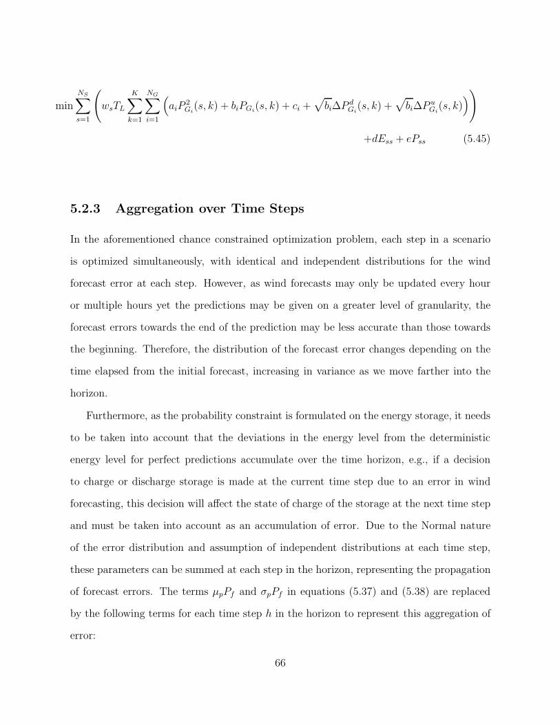
min

NS∑

s=1

(

wsTL

K∑

k=1

NG∑

i=1

(

aiP2Gi(s, k) + biPGi

(s, k) + ci +√

bi∆P dGi(s, k) +

√

bi∆P uGi(s, k)

)

)

+dEss + ePss (5.45)

5.2.3 Aggregation over Time Steps

In the aforementioned chance constrained optimization problem, each step in a scenario

is optimized simultaneously, with identical and independent distributions for the wind

forecast error at each step. However, as wind forecasts may only be updated every hour

or multiple hours yet the predictions may be given on a greater level of granularity, the

forecast errors towards the end of the prediction may be less accurate than those towards

the beginning. Therefore, the distribution of the forecast error changes depending on the

time elapsed from the initial forecast, increasing in variance as we move farther into the

horizon.

Furthermore, as the probability constraint is formulated on the energy storage, it needs

to be taken into account that the deviations in the energy level from the deterministic

energy level for perfect predictions accumulate over the time horizon, e.g., if a decision

to charge or discharge storage is made at the current time step due to an error in wind

forecasting, this decision will affect the state of charge of the storage at the next time step

and must be taken into account as an accumulation of error. Due to the Normal nature

of the error distribution and assumption of independent distributions at each time step,

these parameters can be summed at each step in the horizon, representing the propagation

of forecast errors. The terms µpPf and σpPf in equations (5.37) and (5.38) are replaced

by the following terms for each time step h in the horizon to represent this aggregation of

error:

66

µhPf(h) =

h∑

i=0

µp(i)Pf (i), (5.46)

σhPf(h) =

√

√

√

√

h∑

i=0

(σp(i)Pf (i))2, (5.47)

for h = 0...H − 1.

5.2.4 Discounted Weight on Constraint Violations

Satisfying the chance constraint with probability β becomes increasingly difficult as the

distribution of the forecast error widens. Thus, β will also adapt to account for the current

position in the horizon, decreasing the level of required chance constraint fulfillment. For a

fulfillment probability β ′ at the first time step in the horizon, β will be updated as follows:

βh =β ′

sqrt(h+ 1), (5.48)

for h = 0...H − 1. With this update, the chosen β will capture the same range of values

in the distribution as the original β ′ captured of the original µ′ and σ′, adapting to the

changing distribution parameters.


In this section, we first give an overview over the simulation setup and then discuss the

results.

67

5.3.1 Simulation Setup

We use the IEEE-57 bus test system for the simulations using MATPOWER’s generation

cost parameters and replacing the first of the eight generators with a wind generator.

The 10-minute demand data is taken from ISO New England [22] and the data for the

wind outputs from the Eastern Wind Integration Transmission Study (EWITS) [23]. It

is assumed that the wind predictions in this data are updated every hour and given in

10-minute intervals. The prediction horizon in our simulations is set to one hour at 10

minute intervals, resulting in H = 6. The length of a scenario is one day, resulting in

K = 144. It is assumed that the chosen storage technology is a large lithium-ion battery

with efficiency ηc · ηd = 85% and cost parameters d = $600/kWh and e = $400/kW [13].

In addition, a sensitivity analysis is performed and the optimal storage sizes are given

for a variety of costs and efficiencies. The storage is assumed to be operating without

degradation for the assumed time period of 10 years, i.e., TL = 10 · 365. The computations

were performed using the IBM ILOG CPLEX Optimizer [31] through MATLAB 2013b.

Due to the reformulation of the chance constraint, the optimization problem is now a

convex problem with a quadratic objective and linear constraints. As in Chapter 3, the

CPLEXQP solver was used to solve the optimization.

5.3.2 Optimal Storage Sizing Results

In Table 5.1 the optimal storage parameters Ess and Pss for 20% wind energy penetration by

supplied energy are given, respectively. The number of simultaneously considered scenarios

is set to NS = 10 which already results in over 166,000 variables and 584,000 constraints.

However, the diversity of more scenarios could be captured by using a scenario reduction

technique such as the one described in Chapter 3. The values for optimal storage capacity

are calculated using a constraint satisfaction probability β ′ of one, two, and three standard

deviations away from the mean. As expected, as the constraints on the storage are enforced

68

more stringently, the more advantageous it is to have a larger storage capacity.

Table 5.1: Optimal storage sizes for varying β ′

β ′ Ess(MWh) Pss(MW )

0.68 428.47 46.88

0.95 1566.76 345.15

0.99 2214.75 417.67

An example scenario is shown in Figure 5.3. In Figure 5.4, the optimal power charged/dis-

charged from storage and the state of charge of the storage device for this scenario is given.

The amount of total storage energy capacity, as compared to total demand energy for a

this scenario is 4.96%, and the amount of power capacity of the storage compared to the

peak load is 1.91%. Realistically, this amount of storage in the system would not be con-

tained in one single lithium ion battery, rather, the total capacity requirements would be

dispersed over multiple storage devices in the system.

0 50 100 1500

2000

4000

6000

8000

10000

12000

14000

16000

18000

Time

MW

Total DemandTotal Wind

Figure 5.3: A single scenario.

69

0 20 40 60 80 100 120 1400

200

400

600

800

1000

1200

1400

Time

MW

Power into StoragePower out of StorageStorage Energy Level (MWh)

Figure 5.4: Storage state of charge and power charged/discharged.

5.3.3 Varying Storage Efficiency and Cost

Here, the cost parameters for the energy and power subsystems are varied to study var-

ious battery technologies [13] that could be used for long-duration storage with frequent

discharging. The results are tabulated in Table 5.2 for β ′ = 0.95 and the same 10 scenarios

used previously, starting with the battery used in the previous simulations (lithium-ion).

Table 5.2: Effects of varying the battery technology on the optimal size

BatteryTechnology

ηd · ηc d($/kWh) e ($/kW) Ess(MWh) Pss(MW )

Lithium Ion 85% 600 400 1566.76 345.15

Zinc/Bromine

70% 400 400 3179.27 328.27

VanadiumRedox

65% 600 400 2956.29 262.60

Sodium /Sul-fur

75% 350 350 3290.85 431.73

Lead-acid 80% 330 400 3398.78 466.79

The results for varying the price of the energy capacity of the storage make sense; the

70

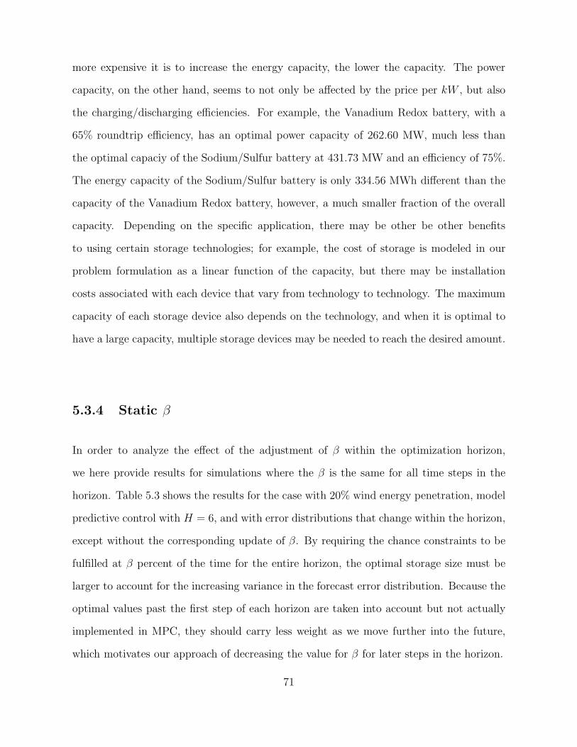
more expensive it is to increase the energy capacity, the lower the capacity. The power

capacity, on the other hand, seems to not only be affected by the price per kW , but also

the charging/discharging efficiencies. For example, the Vanadium Redox battery, with a

65% roundtrip efficiency, has an optimal power capacity of 262.60 MW, much less than

the optimal capaciy of the Sodium/Sulfur battery at 431.73 MW and an efficiency of 75%.

The energy capacity of the Sodium/Sulfur battery is only 334.56 MWh different than the

capacity of the Vanadium Redox battery, however, a much smaller fraction of the overall

capacity. Depending on the specific application, there may be other be other benefits

to using certain storage technologies; for example, the cost of storage is modeled in our

problem formulation as a linear function of the capacity, but there may be installation

costs associated with each device that vary from technology to technology. The maximum

capacity of each storage device also depends on the technology, and when it is optimal to

have a large capacity, multiple storage devices may be needed to reach the desired amount.

5.3.4 Static β

In order to analyze the effect of the adjustment of β within the optimization horizon,

we here provide results for simulations where the β is the same for all time steps in the

horizon. Table 5.3 shows the results for the case with 20% wind energy penetration, model

predictive control with H = 6, and with error distributions that change within the horizon,

except without the corresponding update of β. By requiring the chance constraints to be

fulfilled at β percent of the time for the entire horizon, the optimal storage size must be

larger to account for the increasing variance in the forecast error distribution. Because the

optimal values past the first step of each horizon are taken into account but not actually

implemented in MPC, they should carry less weight as we move further into the future,

which motivates our approach of decreasing the value for β for later steps in the horizon.

71

Table 5.3: Optimal Storage Values without adapting β

β Ess(MWh) Pss(MW )

0.68 993.91 231.79

0.95 3469.08 526.17

0.99 4897.46 624.93

5.3.5 Validation of the Chance Constraint

To verify that the derivation of the chance constraint is correct, a framework for validation

of each chance constraint is constructed. First, because the chance constraint is in terms of

the optimal energy level at each time k, the distribution for the energy level is constructed

based on the wind forecast error distribution, load, and optimal values of the generation

and other storage variables. The parameters of this distribution for every time step k and

scenario s are given first for the chance constraint on the upper limit of the state of charge:

µuE(s, k) = E∗(s, k)−

∆t

ηdP ∗out(s, k) + ∆tµpPf(s, k) + TηcP

∗in(s, k)−∆t

NG∑

i=1

∆P d∗Gi(k)

σuE(s, k) = σp∆tPf (s, k),

and the lower limit on the state of charge:

µdE(s, k) = −E∗(s, k) +

∆t

ηdP ∗out(s, k)−∆tµpPf(s, k)− TηcP

∗in(s, k)−∆t

NG∑

i=1

∆P u∗Gi(k)

σdE(s, k) = σp∆tPf (s, k),

where the asterisk (*) denotes the optimal value, i.e. the solution of the two-stage stochastic

MPC problem. Then, at each step, the percentage of the energy distribution that is outside

the chance constraint limits is calculated. These values were found to satisfy the chance

72

constraint at least β percent of the time for all time steps and scenarios, verifying the

validity of the analytical reformulation of the chance constraint. This concept is seen in

Figure 5.5.

. . .t

0

Validation of Scenario s

Ess

Energy level

. . .

. . .

TN

At the chance constraint limit,(1-)% of energy level distributionis above E ss

Pr(0 ≤ E(t) ≤ Ess) ≥

Figure 5.5: Illustration of the chance constraint validation procedure.

When the energy reaches its upper or lower limit, the chance constraint inequality is

binding. The percentage of time when the chance constraint is binding and the percentage

of time when it is fulfilled with at least probability of 0.99 are listed for varying levels of

β ′ in Table 5.4.

Table 5.4: Chance Constraint Fulfillment

β ′ Percentage of time chanceconstraint is at its limit(binding)

Percentage of time chanceconstraint is fulfilled withprobability ≥ 99%

0.68 13.67% 22.93%

0.95 13.62% 44.87%

0.99 13.85% 100.00%

As the table indicates, the chance constraints are binding about the same percentage

of the time for each value of β. The constraints become binding when the storage is close

73

to its limit or close to zero, which is around the same duration of time in all three cases

(see Figure 5.6). The third column in the table shows the percentage of time the entire

energy distribution is contained within [0, Ess] with at least a probability of 99%. Due

to the increase in storage capacity required to fulfill the case with β ′ = 0.99, the energy

distributions at times when the storage is not at its peak are contained within [0, Ess]

more often than the case with the lower storage capacity corresponding to β ′ = 0.68.

These percentages were calculated over all 10 scenarios. An example scenario is shown in

Figure 5.6 for β ′ = 0.68, 0.95, and 0.99.

As required by the chance constraint, 68%, 95%, and 99% of the energy level distribution

0 20 40 60 80 100 120 1400

2

4

6β = 0.68

0 20 40 60 80 100 120 1400

2

4

6

Ene

rgy

Leve

l (p.

u. ⋅ 1

0−m

ins)

β = 0.95

0 20 40 60 80 100 120 1400

2

4

6β = 0.99

Time

E(k)E

ss

Figure 5.6: Simulation results for the energy levels for varying levels of β.

74

must lie between 0 and Ess. As the requirement becomes stricter, the gap between the

optimal energy capacity and the actual state of charge becomes larger. This goes in line

with the fact that accounting for a larger range of potential forecast errors results in an

increased optimal storage capacity. It is important to note that due to the infinite length

of the tails of the Normal distribution, in order for 100% of the possible forecast errors to

be taken into account, the storage capacity would have to be infinitely large. In reality,

the output of the wind farm would be limited above by its maximum capacity and below

by an output of zero, so these tails would be truncated before infinity in either direction.

However, to account for the cases of wind error that could not be compensated by the

storage and generator ramping, the wind would either have to be curtailed or the power

system reserves would be utilized. In the optimizations here, it is assumed that we want to

utilize as much wind as possible, so curtailing is not an option, although this is an aspect

that could be implemented in the future work.

75

Chapter 6

Coordination Across Control Areas

As electric power systems span entire continents, the control responsibility for these large

systems is shared among multiple entities. Each of these entities is responsible for a specific

geographic area called control area. The coupling of the control areas via tie lines allows

for exchanging power across their boundaries but also leads to the need to coordinate the

actions in the areas. Traditionally, this is being done by agreeing on a tie line flow, e.g.

based on market mechanisms, and then optimize the schedule of generation within the

areas to balance supply and demand. This leads to a potentially suboptimal usage of the

available resources because the optimization is limited to the localized areas.

As long as resources are distributed throughout the system in a fairly homogenous way

in terms of their capabilities and costs, the suboptimality may be acceptable. However,

once the resources in one area have considerably different characteristics compared to the

resources in the neighboring area, substantial improvements in terms of providing reliable

and cost effective electric power supply may be achieved. In this thesis, we particularly

consider the situation in which one area has significant amounts of variable renewable

generation resources and the other area has significant amounts of storage.

In that case, it is beneficial for both areas to improve the coordination such that the

storage is being used to balance the variability of the renewable resources. Generally, this

77

means that the control areas should be optimized jointly in a single centralized optimization

problem requiring that the areas share their system information either with the other

entities or a centralized entity overseeing all areas. Another option is to use decomposition

techniques to decompose the centralized problem into subproblems each associated with

a particular control area. The result is an iterative process where each area solves the

problem assigned to it and then provides some information about the solution at the buses

located at the boundary of the area to the other areas. Based on the information received

the areas update their solution and keep exchanging until convergence has been achieved.

The final solution should be equal to the solution obtained if the problem would be solved

by a centralized entity across all areas.

MPC has previously been applied to power systems for energy storage control. In [45]-

[48], centralized MPC is used on relatively small scale systems to optimally control a battery

to reduce the effect of fluctuations in the power supply due to renewable generation. In [49],

a multi-time period DC OPF problem with storage is solved in a distributed way using the

alternating direction method of multipliers (ADMM), where devices that exchange energy

are required to exchange information in a peer-to-peer framework. The nonconvex MPC

AC OPF problem is solved in a distributed manner in [50] using the AND method on

the IEEE-14 bus test system. The work shown in [50] is extended in this chapter to the

IEEE-57 bus test system, and two modifications on the AND method aiming to improve

the rate of convergence are used to solve the distributed optimization. Distributed MPC

is implemented for another purpose in [51] for Automatic Generation Control, and in [52]

for the mitigation of cascading failures in a power system.

In this thesis, distributed MPC is used to coordinate renewable generation in one area

with storage in another area. Two extensions are derived for the original AND method

which for a variety of cases significantly improve the rate of convergence of the optimization.

Simulation results are given for the IEEE-57 bus test system (parameters for the system

78

are found in the Appendix). Generally, solving the AC OPF problem for each step in an

entire prediction horizon results in a very large nonlinear optimization problem; however,

the straightforward decomposition of the problems using AND makes the optimization

of the individual subproblems easily parallelizable. When this method is applied to the

multi-area OPF problem as in [53] and [50], the variables exchanged between the areas

corresponds to the voltage magnitudes and angles at buses connected across areas, as

well as the Lagrange multipliers at these connected buses and lines. The Lagrangian

multipliers are directly given from the neighboring subproblems, unlike other Lagrangian-

based decomposition methods which require a separate update for the Lagrange multipliers.

There is no need for areas to share information with other areas that is not related to their

physically connected buses, and the problem converges to the centralized solution provided

the convergence criteria is met [4].

6.1 Problem Formulation

The problem that we address in this chapter is a Model Predictive Control problem to

minimize the overall cost of supplying the load and balancing fluctuations in the power

supply introduced by wind by optimally utilizing the available energy storage. Hence, it is

a multi-step optimal power flow problem which is subject to inter-temporal constraints on

energy storage devices and the AC power flow constraints. The overall problem formulation

is therefore given by

minN∑

k=1

(

NB∑

i=1

aiP2Gi

+ biPGi+ ci

)

(6.1)

s.t. PGi(k) + PWi

(k)− PLi(k) (6.2)

− Pini(k) + Pouti(k)−

∑

j∈Ωi

Pij(k) = 0, (6.3)

79

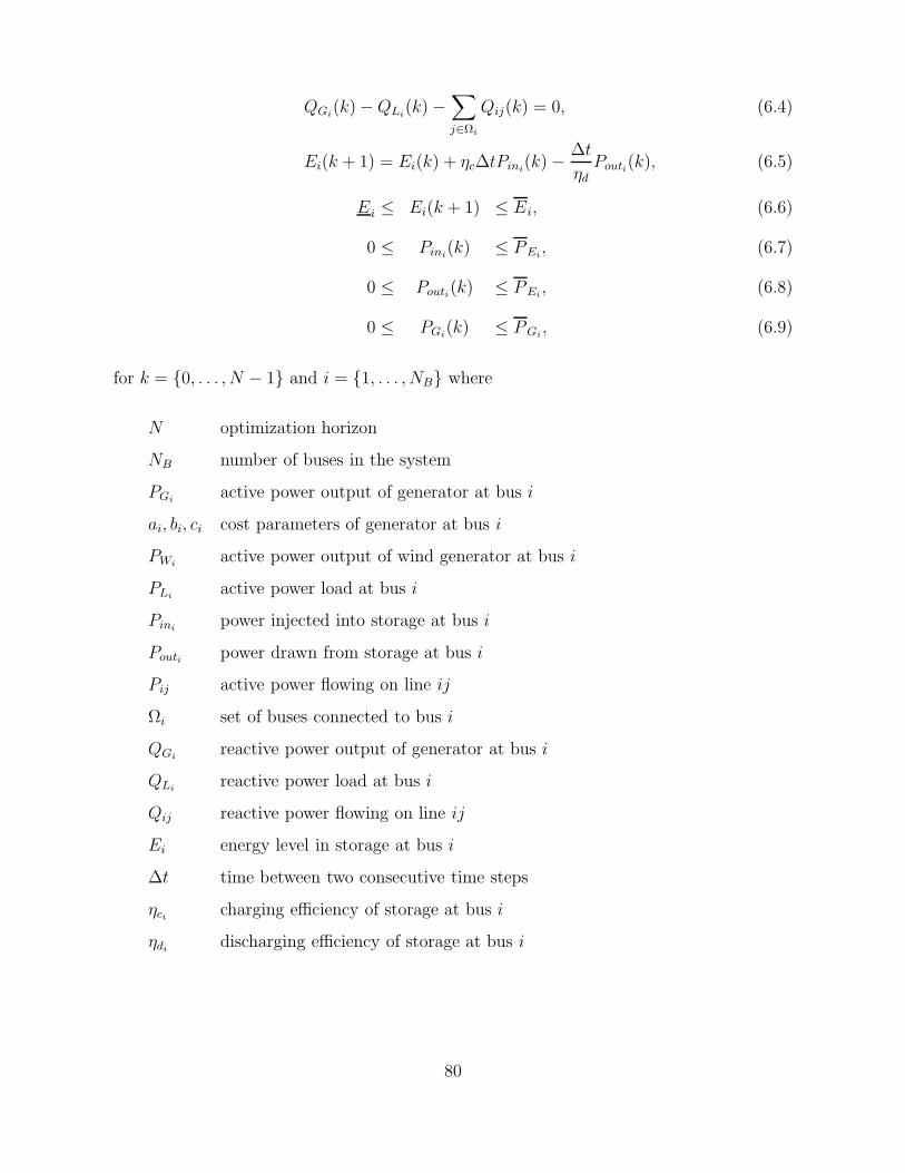
QGi(k)−QLi

(k)−∑

j∈Ωi

Qij(k) = 0, (6.4)

Ei(k + 1) = Ei(k) + ηc∆tPini(k)−

∆t

ηdPouti(k), (6.5)

Ei ≤ Ei(k + 1) ≤ Ei, (6.6)

0 ≤ Pini(k) ≤ PEi

, (6.7)

0 ≤ Pouti(k) ≤ PEi, (6.8)

0 ≤ PGi(k) ≤ PGi

, (6.9)

for k = 0, . . . , N − 1 and i = 1, . . . , NB where

N optimization horizon

NB number of buses in the system

PGiactive power output of generator at bus i

ai, bi, ci cost parameters of generator at bus i

PWiactive power output of wind generator at bus i

PLiactive power load at bus i

Pinipower injected into storage at bus i

Pouti power drawn from storage at bus i

Pij active power flowing on line ij

Ωi set of buses connected to bus i

QGireactive power output of generator at bus i

QLireactive power load at bus i

Qij reactive power flowing on line ij

Ei energy level in storage at bus i

∆t time between two consecutive time steps

ηci charging efficiency of storage at bus i

ηdi discharging efficiency of storage at bus i

80

PGimaximum active power output of generator at bus i

Ei lower energy limit of storage at bus i

Ei energy capacity of storage at bus i

PEimaximum dis/charging rate of storage at bus i

Whenever there is no generator connected to bus i, it is assumed that equations (6.2)

– (6.4) are reduced to not include the generation output variable. The same holds for the

wind generator output, the loads and the storage variables. Equalities and inequalities

(6.5) – (6.9) are only included if there is a generator or a storage connected to bus i.

Equations (6.2) – (6.4) represent the power flow equations in the system where the flows

Pij and Qij are given as follows:

Pij = |Vi| |Vj| (Gij cos θij +Bij sin θij),

Qij = |Vi| |Vj | (Gij sin θij −Bij cos θij),

(6.10)

where Vi and Vj are the voltage magnitudes at bus i and bus j respectively, θij is the

voltage angle difference between buses i and j, Gij is the real part of the admittance

matrix element yij, and Bij is the imaginary part of yij.

As Model Predictive Control is used here, once the problem (6.1) – (6.9) is solved for

time step t, the solution for the first step k = 0 is applied. Then, the optimization horizon

is shifted by T and the problem is solved for the new time horizon.

6.2 Distributed MPC

The resulting optimization problem (6.1) – (6.9) corresponds to the centralized problem

including multiple control areas. Decomposing the problem allows each control area to

solve the optimization problem associated with its own part of the system while optimally

coordinating with its neighboring areas. Hence, the main motivation for decomposing

the problem in this work is to enable the optimal coordination across areas. However,

81

decomposition of the considered problem generally allows for parallelized computations

and therefore for solving large scale optimization problems which otherwise could not be

solved or not solved within a reasonable amount of time. As the prediction horizon N

increases, the considered MPC problem may lead to such a large scale problem and despite

the potentially existing centralized coordinator could require a distributed solution process.

In this thesis, we consider two modifications of the Approximate Newton Directions

(AND) method, both with the intention to reduce the gap between the distributed variable

update and the centralized update, thus improving the convergence rate in some cases. The

problem is first decomposed using Optimality Condition Decomposition (OCD) and then

the resulting optimization problem is solved in a distributed manner using AND method

as well as solved using the two modifications presented here. The advantage of using

this method over other Lagrangian-based decomposition methods is that there is no need

for a centralized controller, and the Lagrange multipliers are updated directly from the

other subproblems. After the problem is decomposed, the coupled variables are exchanged

between subproblems during each Newton-Raphson iteration; there is no need for each

subproblem be solved until optimality before exchanging values. In the optimal power

flow problem, these coupling variables correspond to the voltage magnitudes and angles

at the border buses between control areas, and the decomposition into subproblems is

straightforward. The details of the OCD and AND method are discussed in more depth in

Chapter 2.

6.2.1 Jacobi Update Method

The first modification is derived from the Jacobi method for solving a linear system of

equations [57]. Instead of setting the off-diagonal block matrices in the Jacobian matrix

to zero, the information from the previous iteration p − 1 is used to update the variables

82

at iteration p. The variable update for each subproblem p = 1, . . . ,M is now equal to

J (p)q,q ·∆x(p)

p = −d(p)q −M∑

m=1,m6=q

(J (p−1)m,q ·∆x(p−1)

m ), (6.11)

where Jq,q is the on-diagonal Jacobian corresponding to subproblem q and Jm,q is the off-

diagonal Jacobian corresponding to the partial derivatives of the constraints in subproblem

m with respect to the variables in subproblem q. The structure of the overall Jacobian can

be seen in section 2.3. Even with these additional terms in the update it is not necessary to

exchange the full update vectors ∆x(p−1)m among the areas. Area m can, without additional

information exchange, evaluate J(p−1)m,q at iteration p−1 and then compute the multiplication

with the update vector ∆x(p−1)m . As J

(p−1)m,q is very sparse, the multiplication with ∆x

(p−1)m

results in a sparse vector and only the non-sparse elements need to be shared.

The issue with this update is that it basically builds upon the assumption that ∆x(p−1)m

and ∆x(p)m will be similar, which does not necessarily have to be the case and may therefore

only result in improved performance in certain cases.

6.2.2 Additional term in Right Hand Side Vector

The second approach is a bit more involved in its derivation. Hence, we use a two area

example to present the main idea. The centralized update is given by

J(p)11 J

(p)12

J(p)21 J

(p)22

·

∆x(p)1

∆x(p)2

= −

d(p)1

d(p)2

(6.12)

By reordering the terms in the rows, the following formulae for the updates result,

∆x(p)1 = −J

(p)−1

11 · d(p)1 − J(p)−1

11 J(p)12 ·∆x

(p)2 , (6.13)

83

∆x(p)2 = −J

(p)−1

22 · d(p)2 − J(p)−1

22 J(p)21 ·∆x

(p)1 . (6.14)

By substituting (6.14) into (6.13) and vice versa, the updates can be written as a function

of the matrices and the right hand side vectors, i.e. (for simplification, we do not indicate

the iteration counter in these equations)

∆x1 = (J11 − J12J−122 J21)

−1 · (−d1 + J12J−122 · d2), (6.15)

∆x2 = (J22 − J21J−111 J12)

−1 · (−d2 + J21J−111 · d1). (6.16)

This update corresponds to the exact update, i.e. the update that is obtained if Newton

Raphson is applied to the first order optimality conditions of the centralized problem. As

can be seen, even for two areas, a fairly complicated update results if this is to be done in

a distributed way. Consequently, we propose to simplify this update to

∆x(p)1 = J

(p)−1

11 · (−d(p)1 + J

(p)12 J

(p)−1

22 · d(p)2 )

= J(p)−1

11 · (−d(p)1 + d

(p)12 ) (6.17)

∆x(p)2 = J

(p)−1

22 · (−d(p)2 + J

(p)21 J

(p)−1

11 · d(p)1 )

= J(p)−1

22 · (−d(p)2 + d

(p)21 ) (6.18)

This update is significantly less computationally intense than (6.15) – (6.16). Area 1

can compute d(p)21 without additional knowledge from area 2 and then provide area 2 with

the non-zero entries in this vector. The computation of d(p)21 involves the inverse of J

(p)11 .

However, that inverse is needed for the update of ∆x(p)1 anyway. Consequently, area 1 can

reuse the inverse for the computation of d(p)21 . Generally, there should only be very few terms

in the vectors d(p)1 and d

(p)2 which are non zero, namely the ones which correspond to first

order optimality constraints which include variables from both subproblems. Hence, only

a limited amount of additional information needs to be exchanged among the subproblems

84

(not the entire additional vector) to carry out (6.17) and (6.18). We now generalize the

update for the case with multiple areas. Hence, we propose the following update

∆x(p)q = J (p)−1

q,q · (−d(p)q +

M∑

m=1,m6=q

J (p)q,mJ

(p)−1

m,m · d(p)m )

= J (p)−1

q,q · (−d(p)q +M∑

m=1,m6=q

d(p)q,m) (6.19)

With the communication of these few extra terms, the updates carried out locally for the

areas is closer to the centralized update. Hence, it can be expected that the number of

iterations until convergence is reached is reduced compared to the original method or the

method with the modification based on the Jacobi update.


The IEEE-57 bus system is decomposed into two geographical regions as shown in Figure

6.1. Two wind generators are placed at buses 17 and 43, and a storage device with roundtrip

efficiency of ηc · ηd = 0.95%, standby loss of 0.005p.u.·10-minutes and maximum capacity

of 0.5p.u.·10-minutes is placed at bus 7. Simulations were run for a 24-hour period with

prediction horizons of N = 1, 3, 6 and 9 where T = 10min, hence, the horizon length

correspond to no horizon, 30-minute, 60-minute, and 90-minute horizons. There is a 27%

level of wind energy penetration in the system by energy. The cost functions and maximum

output limits for the generators were obtained from the IEEE-57 bus specifications in

MATPOWER [44] and tabulated in the Appendix. Here, the storage is operated at the

10-minute scale to balance out the intra-hourly fluctuations in the power supply caused by

variations in the wind and load. Storage could also be used with this method on an hourly

scale for longer term load shifting applications. Historical data for the wind and load was

used from ISO New England and for the particular simulation presented here the load and

85

G

G

G

G G

G

G

12

3

4

5

6

7

8 9

10

11

12

13

14

15 16

17

18

19 20

21

22

23

24

25

26

27

28

29

30

3132

3334

35

36

37

38

39

40

41

42

43

44

45

46

47

48

49

50

51

52

53

54

55

56

57

S

W

W

G

G

G

G G

2

3

4

5

6

7

8 9

18

19 20

211

22

223

224

25

26

227

288

229

52

53

5554

55

S

GGG

G

1

10

11

12

13

14

15 16

17

3000

3132

333334

35

36

37

3338

39

40

41

42

4333

4444

445

466

47

488

49

50

51

556

57

W

WW

3

020

30

Area 1

Area 2

Figure 6.1: IEEE-57 bus system decomposed into two areas

wind curve as given in Fig. 6.2 are used.

The results were compared with the solution of the centralized problem achieved by the

SNOPT solver in the commercial optimization package TOMLAB and found to be within

1e−3 of the solution. The algorithm is considered to have converged once the maximum

absolute value over all elements in the vector of the first order optimality conditions d is

less than 1e−4. It is important to note that in these simulations, because this is a proof of

concept simulation, the predictions for the wind are assumed to be perfect; i.e., there is no

forecast error, and a longer horizon always results in a lowered objective function value.

This may not necessarily be the case if prediction errors are considered. With prediction

86

0 20 40 60 80 100 120 1400

0.2

0.4

0.6

0.8

1

1.2

1.4

Timestep (10−minute Increments)

p.u.

Total System LoadTotal System Wind

Figure 6.2: 24-Hour input data with 10-minute intervals

errors the results depend on the level of the prediction error.

6.3.1 Existence of Local Minima

Due to the nonconvexity of the AC OPF problem, there is a chance that the result of

the optimization may be a local optimum. There exist global optimization techniques

for specific formulations of AC OPF [55], [56], but there are currently no techniques for

finding the global optimum of the distributed Model Predict Control AC OPF problem

considered in this thesis. However, if local minima are encountered, they usually correspond

to physically infeasible situations [54]. In these simulations, we first solve a standard AC

power flow and use the resulting voltage magnitudes and angles as the starting point for the

optimal power flow calculation. The subsequent time steps, after shifting the horizon, use

the solution from the previous optimization as the initial point. The same starting points

were used when comparing with the SNOPT solver and confirmed to reach the same final

solution.

87

6.3.2 Effect of Optimization Horizon

Figure 6.3 shows the power charged/discharged from the storage device over the 24-hour

period, and Figure 6.4 shows the state of charge of the storage over the 24-hour period.

The longer the horizon, the better is the utilization of the energy storage as longer term

variations in net load can be predicted and be accounted for. The effect is that less ramping

is need from the generators as can be seen in Fig. 6.5, where the total generation output

from dispatchable generators is shown for the horizon N = 9. It should be noted that as

AC power flow is used, the overproduction in generation is mostly due to AC power flow

losses.

The total amount of generator ramping summed over all individual generators was

measured for each horizon N = 1 (no MPC), 3, 6, and 9 and the total generation costs

were calculated. As indicated by the results shown in Table 6.1, with the use of MPC,

the overall required amount of generator ramping decreases. Without the use of storage,

generators must adjust their output more frequently to account for the fluctuations in the

power supply introduced by the wind. The reduction in overall generation cost for the

considered day and compared for the different horizon lengths is quite low. However, that

measure heavily depends on the particular load and wind curves for the considered day

as well as the composition of the generators, i.e. which generators become the marginal

generators and which reach their capacity limit. Also note that this does not say anything

about the difference in cost if coordination is used and if it is not. The comparison solely

is focused on the different lengths in horizon. As this thesis focuses on the method of

how to coordinate the areas, a full economic analysis is beyond the scope of this thesis.

However, it can be expected that the greater the differences in cost parameters and the

higher the fluctuations in net load are, i.e. the higher the penetration of variable renewable

generation, the higher the benefit of longer horizons.

88

0 20 40 60 80 100 120 140−0.1

−0.05

0

0.05

0.1


p.u.

N = 3 (30 minutes)N = 6 (60 minutes)N = 9 (90 minutes)

Figure 6.3: Optimal power input (positive) and output (negative) from storage

0 20 40 60 80 100 120 1400

0.1

0.2

0.3

0.4

0.5


p.u.

⋅ 10

−m

inut

es

N = 3 (30 minutes)N = 6 (60 minutes)N = 9 (90 minutes)

Figure 6.4: Optimal state of charge of storage device

0 20 40 60 80 100 120 140

0.2

0.4

0.6

0.8

1

1.2


p.u.

Total Net LoadTotal Generation Output

Figure 6.5: Optimal generation levels for N = 9

89

6.3.3 Comparison of Convergence Rates

Requirement for Convergence

In order for the AND method to converge to the optimal solution x∗ of the problem

described in (6.1) – (6.9), the following must hold true at the optimal solution [4]:

ρ(I − Jdec · Jtot) < 1 (6.20)

where ρ indicates the spectral radius. Matrix Jtot is the Jacobian matrix (2.11) evaluated

at the optimal solution and Jdec is the Jacobian matrix with off-diagonal elements set to

zero again at the optimal solution. If the condition on the spectral radius is not fulfilled,

the optimization may be unable to converge to the optimal solution. In these cases, a

preconditioned conjugate gradient method such as the generalized minimal residual method

(GMRES) [57] may be used to improve the convergence. In the system decomposition

used in this example, the spectral radius was calculated to be around 0.88, fulfilling the

convergence criteria. This value was not found to change dramatically depending on the

horizon length or point in the simulation for the considered case.

Comparison of Distributed Methods

In Table 6.2, the minimum, maximum, and median number of iterations to convergence

for each method for horizons N = 1, 3, 6 and 9 is shown. Figure 6.6 shows the rate of

Table 6.1: Required Generator Ramping and Total Generation Cost

N 1 3 6 9

Total Generator

Ramping (p.u.) 2.29 1.88 1.73 1.53

Total Generation

Cost ($) 587,235 587,003 586,716 586,568

90

convergence at simulation timestep t = 2 for each of the three distributed optimization

methods for N = 9. To ensure better convergence properties at the cost of a higher

number of iterations, the damping parameter α on the Newton-Raphson step was initially

chosen to be 0.25. In the rare cases where the method still continued to diverge, a higher

damping of 0.1 was chosen for the iterations which leads to a few outliers in terms of

iteration numbers. To reduce the number of iterations, an adaptive approach for setting

the damping parameter could be used. For the sake of comparison, the same damping

factors have been used throughout the iteration process for a particular time step.

As the results indicate, the Jacobi update method only leads to significant improvements

for N = 1, whereas the method with the additional term leads to significant reduction

for horizons of N = 1 and N = 9 and stays roughly the same for the other horizons.

The conclusion that can be drawn is that an analysis should be done for the particular

considered problem to determine whether or not it is useful to add in the additional term.

0 100 200 300 400 500 60010

−5

100

105

Number of Iterations

Nor

m o

f KK

T V

ecto

r(D

ista

nce

from

Sol

utio

n)

Original ANDJacobi UpdateAdditional Term

Figure 6.6: Convergence rates for N=9

91

Table 6.2: Number of Iterations to Convergence

Method N

Minimum

Iterations to

Convergence

Median

Iterations to

Convergence

Maximum

Iterations to

Convergence

Original AND 1 356 511 704

Jacobi Update 1 360 364 642

Additional Term 1 337 363 500










92

Chapter 7

Jacobian Singularities

With problem formulations that contain constraints that span over multiple time steps,

i.e., intertemporal constraints, singularities in the Newton-Raphson Jacobian may occur.

This happens frequently with the aforementioned storage model, and may happen with

other intertemporal constraints commonly encountered in power system optimization such

as generator ramp limits, for example. This section identifies when these singularities occur

and develops techniques used to find a solution to the optimization problem in the presence

of Jacobian singularities.

7.1 Causes of Singularities

Previously, singular Jacobian matrices in Newton-Raphson based load flow calculations

were found to be related to situations near voltage collapse [58, 59]. This dissertation ad-

dresses another instance of singular Jacobians in power system optimization; those related

to intertemporal constraints such as generator ramp limits and specifically, the storage

model given in (3.1) - (3.4). When all of these storage constraints become binding, the

Jacobian of the first-order optimality conditions may become singular. This case occurs

when the set of binding intertemporal constraints have linearly dependent gradients at

93

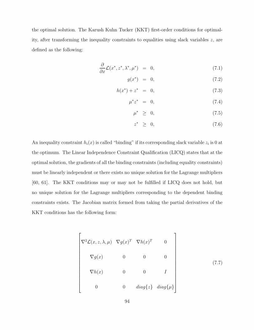
the optimal solution. The Karush Kuhn Tucker (KKT) first-order conditions for optimal-

ity, after transforming the inequality constraints to equalities using slack variables z, are

defined as the following:

∂

∂xL(x∗, z∗, λ∗, µ∗) = 0, (7.1)

g(x∗) = 0, (7.2)

h(x∗) + z∗ = 0, (7.3)

µ∗z∗ = 0, (7.4)

µ∗ ≥ 0, (7.5)

z∗ ≥ 0, (7.6)

An inequality constraint hi(x) is called “binding” if its corresponding slack variable zi is 0 at

the optimum. The Linear Independence Constraint Qualification (LICQ) states that at the

optimal solution, the gradients of all the binding constraints (including equality constraints)

must be linearly independent or there exists no unique solution for the Lagrange multipliers

[60, 61]. The KKT conditions may or may not be fulfilled if LICQ does not hold, but

no unique solution for the Lagrange multipliers corresponding to the dependent binding

constraints exists. The Jacobian matrix formed from taking the partial derivatives of the

KKT conditions has the following form:

∇2L(x, z, λ, µ) ∇g(x)T ∇h(x)T 0

∇g(x) 0 0 0

∇h(x) 0 0 I

0 0 diagz diagµ

(7.7)

94

The consequences of having dependent binding constraints; i.e., having the LICQ unsatis-

fied, can be seen by analyzing the following rows of the Jacobian:

∇g(x) 0 0 0

∇h(x) 0 0 I

0 0 diagz diagµ

(7.8)

When the gradients of the constraints are linearly dependent and the constraints are bind-

ing, the above rows are linearly dependent. This is due to the fact that when a constraint

i is binding, zi = 0 and µi 6= 0. Thus, if ∇g(x) and ∇h(x) are dependent when binding,

this entire matrix block (7.8) will have dependent rows due to z = 0 and µ 6= 0.

Also, a row of zeros could also be created by the possibility that µi and zi could both

become 0. These are two ways that the matrix could become singular by violating LICQ.

In the considered problem, this occurs when the optimal usage of the storage device is such

that it is at its minimum or maximum capacity for two consecutive timesteps and there is

no charging or discharging from the device.

7.2 Approaches to Solving the Singularity Problem

7.2.1 Moore-Penrose Pseudoinverse

There are multiple ways that the singular Jacobian problem can be addressed. Because

it is known that the Jacobian is singular at the optimal solution and it is not a result of

numerical issues, one way that the underdetermined system of equations can be solved is

by using a Moore-Penrose pseudoinverse. The formula for Newton-Raphson with Jacobian

matrix J and vector of KKT condtions f at iteration i can be written in this form:

95

J(xi) ·∆xi = −f(xi). (7.9)

For simplicity, the above system of equations will henceforth be referred to as Ax = b,

where the Jacobian matrix J is the A matrix in this case. The pseudoinverse A+ is defined

as [62]:

A+ = UΣ+V T , (7.10)

with Σ+ = diag(σ−11 , ...σ−1

r , 0, ..., 0); where σ1...σr are the singular values of ATA, and U

and V are matrices with orthonormal columns. This A+ is the same pseudoinverse as given

by the MATLAB command pinv.

The solution achieved by using this pseudoinverse is given by:

x+ = A+b, (7.11)

where this solution, x+, solves the underdetermined linear least squares (minimum norm)

problem. The optimal solution to this problem, that is, the minimum norm solution, is

x∗. Since the system is underdetermined and multiple solutions exist, at a solution x∗,

Ax∗ = b. It can be shown [63] that x+ = x∗ and thus using this pseudoinverse to solve

(7.9) will yield a solution to the KKT conditions; i.e., the solution fulfills (7.1)-(7.6).

7.2.2 Storage Standby Losses

Another approach is to avoid the Jacobian becoming singular altogether. Introducing

storage losses provide a solution which will render the Jacobian matrix non-singular. This

loss could represent inertia losses from a flywheel or charge leakage from a lithium-ion

battery, for example. There are two possible methods by which these losses could be

included:

96

i. Subtractive Standby Losses

A constant standby loss term ǫ can be subtracted from the energy balance equation

to represent energy losses from elapsed time rather than just including charging/dis-

charging losses. The new storage formulation can be written as

E(t + T ) = E(t) + ηcTPin(t)−T

ηdPout(t)− ǫL. (7.12)

This loss will prevent all of the intertemporal constraints related to this storage device

to be simultaneously binding. For example, if the following constraints are binding:

E(t) = Emin, (7.13)

Pin(t) = 0, (7.14)

Pout(t) = 0, (7.15)

then because of the standby losses, at time t + T , the energy level would dip below

Emin. Thus, Pin(t), the power into the storage, must be nonzero to avoid the en-

ergy level going below its minimum. When the energy level E(t) is at its maximum,

E(t + T ) cannot also be at its maximum in the next time step unless Pin(t) 6= 0.

Hence, because of the standby losses, all of these storage constraints are prevented

from being simultaneously binding.

ii. Multiplicative Standby Losses

The losses can also be modeled as a percentage loss:

E(t + T ) = ǫNE(t) + ηcTPin(t)−T

ηdPout(t). (7.16)

97

However, it is important to note that if the minimum storage level Emin is 0, this

model can still result in simultaneously binding constraints. This is because when

E(t) = 0, and all other storage constraints are binding (Pin(t) = Pout(t) = 0), the

term ǫNE(t) will still be 0; i.e., the storage will not need to feed in power to account

for standby losses and all of the storage constraints can become binding.

In both of the above methods for incorporating standby losses, rare cases can occur

that still result in Jacobian singularities. For example, if E(t) = Emin, Pin(t) = Pmaxin ,

Pout(t) = 0, and E(t + T ) = Emax; i.e., the storage is initially empty and wants to charge

at its maximum rate for the current step. The value for the maximum charging rate must

exactly result in the storage being at Emax after the time interval T . In this case, standby

losses do not help, and it is possible for the constraints to all be binding. However, cases

such as this are rare and presumably will not be frequently encountered.

7.2.3 Constraint/Variable Removal as Intertemporal Constraints

Approach Binding

The third approach to avoid singular Jacobian matrices is to remove the rows that corre-

spond to linearly dependent constraints and solve the resulting linearly independent system

of equations. A priori, it is not known which, if any, of the intertemporal equations will

be binding. By analyzing the structure of the Jacobian, however, we can deduce that

once these constraints become binding, they will stay binding. Having constraint gradients

that are linearly dependent means that we can remove constraints from the constraint set

without affecting the solution, a principle which is used in active set methods [64].

Analyzing the structure of (7.9), we see that the Newton-Raphson step has the following

form:

98

∇2xxL ∇g(x)T ∇h(x)T 0

∇g(x) 0 0 0

∇h(x) 0 0 I

0 0 diagz diagµ

∆x

∆λ

∆µ

∆z

=

∇xL

g(x)

h(x) + z

diagµ · z

For a particular slack variable zi, we see that:

zi ·∆µi + µi ·∆zi = µi · zi. (7.17)

Assuming µi at the current step is nonzero, if zi = 0, then in order for this equation to

hold, ∆zi must be zero. Thus, zi will not change during future iterations. This fact will be

used to identify the storage constraints which already become binding at their optimum

during the Newton-Raphson iterations. We then use this to remove constraints to ensure

that the Jacobian matrix will not become singular as we continue the iterations.

To see the implications of a binding constraint in the context of the storage constraints,

we can examine the KKT conditions relating to the storage constraints. In the case of the

storage being empty, for example, we can examine the transformed inequality constraints,

−E(t) + Emin + zl = 0, (7.18)

−Pin(t) + zo = 0, (7.19)

−Pout(t) + zp = 0, (7.20)

and see that if any of the slack variables are zero, it implies that that variable is at its

minimum. To ensure that these constraints are satisfied when the slack variables become

99

zero, a check must also be done to determine if the variables Pin(t), and Pout(t) are at their

minimum, and E(t+T ) and E(t) are both at their minimum or both at their maximum as

well. Numerically, these variables may not actually reach exactly zero, so the comparison

for implementation purposes is done with a tolerance ǫ that is close to zero. For the rare

case when both µi(t) and zi(t) become zero at the same time, the Jacobian will become

singular because a row of zeros is created. To avoid this case, certain measures can be

taken such as running the optimization from a different starting point or using a smaller

damping value on the Newton-Raphson step.

Overall, the steps to indicate whether or not to remove the rows corresponding to the

storage device constraints and actually remove corresponding rows and columns are as

follows:

1. Determine if (|E(t)−Emin| or |E(t)−Emax|), (|E(t+T )−Emin| or |E(t+T )−Emax|),

|Pin(t)|, and |Pout(t)| < ǫ.

2. Determine if the slack variables z(t) corresponding to the above variables are all less

than ǫ.

3. If 1) and 2) are true, remove the following elements of the Jacobian:

(a) The rows and columns in the ∇2xxL block that correspond to the partial deriva-

tives of E(t), Pin(t), and Pout(t).

(b) The rows and columns corresponding to the gradients of the binding storage

constraints at time t.

(c) The rows and columns in diagµ · z that include µ(t) and z(t) for the corre-

sponding inequality constraints.

4. Replace instances of variables E(t), Pin(t), and Pout(t) where they appear in the rest

of the Jacobian matrix with their optimal values.

100

5. Adjust the KKT conditions in the right-hand side vector of the update to no longer

include constraints (3.1)-(3.4), partial derivatives of the Lagrangian with respect to

the storage variables, or complementary slackness conditions diagµ(t) · z(t).

6. Repeat for each time instance considered in the optimization; i.e., for the entire

problem time horizon t = 0, ..., N − 1.

7. Perform the Newton-Raphson step with the reduced Jacobian and right-hand side

vector.

Depending on the application and purpose, some of these methods may be more ap-

propriate than others. For example, using a Moore-Penrose pseudoinverse may be more

computationally complex and require more computation time than other methods. It also

requires that either the rank or condition number of the Jacobian is checked each iteration

to determine if the Jacobian is close to singular. Integrating storage standby losses may

not only fix the singularity of the Jacobian, but may also provide a more realistic model

of a storage device.

However, this does require a modification of the model, and if the standby losses are too

small, the matrix may still be close to singular and numerically unstable. Also, in some

rare cases, even with standby losses, all of the storage inequalities can still be binding,

as discussed above. The technique of removing the binding constraints/variables has the

benefit of reducing the size of the Jacobian matrix and hence potentially reducing the

number of computations per Newton step; however, this method also has the downside

of deciding the tolerance parameter ǫ. If the constraints are removed prematurely and

they actually are not binding at the optimal solution, the KKT conditions may not be

satisfied, and if they are removed too late, the Jacobian may already be close to singular,

resulting in numerical issues. In this case, using a pseudoinverse may result in more robust

performance.

101


In this section, results are shown for AC OPF simulations on the IEEE 14 bus system [65].

System details are to be found in the Appendix. Wind generators, modeled as negative

loads, have been added at buses 5 and 14, and a storage device has been added at bus 5 as

seen in Figure 7.1. The objective is to minimize the quadratic cost of generation from the

generators at buses 1, 2, and 3. Simulations were done over a period of 24 hours, with a

5-minute discretization and prediction horizons N = 5 and N = 10. The receding horizon

concept is used, where the optimization is performed over the time horizon N , variables

are updated, and the time window is shifted and the process is repeated.

The formulation of the KKT conditions is modified to incorporate the Unlimited Point

Algorithm [12], which is a technique to ensure the non-negativeness of µ and z by raising

these variables to an even power, as explained in Chapter 2. In our simulations, we have

squared µ and z where they appear in the KKT conditions, keeping the complementary

slackness condition diagµ · z = 0 the same, because it is equivalent to diagµ2 · z2 = 0.

The modified Jacobian is shown below:

∇2xxL(x, z, λ, µ)∇g(x)T 2∇h(x)T · diagµ 0

∇g(x) 0 0 0

∇h(x) 0 0 2diagz

0 0 diagz diagµ

(7.21)

This does not change the singularity problem, as the dependent binding constraints still

result in these rows being linearly dependent. Other methods to account for the positivity

of µ and z, such as using an interior point or barrier method, result in the same issues. Thus

the given methods to fix the singularities were explained for the general KKT conditions

102

in (7.1)-(7.6), but it is important to note that these singularities still exist even when using

the Unlimited Point or Interior Point method. In the following simulations, we use the

method of removing the rows of the Jacobian which cause the singularity issue.

G

G

G

CC

1

2

12

13

14

11

10

6

5

3

9

4

78

W

S

W

G

C

Generator

Synchronous

Condenser

W

S

Wind plant

Storage Device

Figure 7.1: Modified IEEE 14-bus System

Data for the wind and load curves were taken from the Bonneville Power Administration

[42]. One simulation output for the energy level of the storage device over a 24-hour period

with N = 5 is seen in Figure 7.2. The storage device has a minimum required capacity of

0.2p.u. and a maximum capacity of 1.2p.u. The storage level for this horizon length never

reaches its maximum; however, with longer horizons, the storage is utilized more and does

reach its maximum value, as seen in Figure 7.3. The storage is utilized to balance out the

intermittency of the wind generators in attempts to keep controllable generators at a more

constant level without having to ramp up and down.

For the cases of horizons N = 5 and N = 10, instances where the constraints (3.1)-

(3.4) were found to be simultaneously binding for at least one time instance within the

103

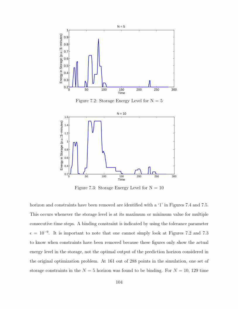
0 50 100 150 200 250 3000.2

0.3

0.4

0.5

0.6

0.7

0.8

0.9

1N = 5

Time

Ene

rgy

in S

tora

ge (

p.u.

⋅ 5−

min

utes

)

Figure 7.2: Storage Energy Level for N = 5

0 50 100 150 200 250 3000.2

0.4

0.6

0.8

1

1.2

1.4

1.6N = 10

Time

Ene

rgy

in S

tora

ge (

p.u.

⋅ 5−

min

utes

)

Figure 7.3: Storage Energy Level for N = 10

horizon and constraints have been removed are identified with a ‘1’ in Figures 7.4 and 7.5.

This occurs whenever the storage level is at its maximum or minimum value for multiple

consecutive time steps. A binding constraint is indicated by using the tolerance parameter

ǫ = 10−9. It is important to note that one cannot simply look at Figures 7.2 and 7.3

to know when constraints have been removed because these figures only show the actual

energy level in the storage, not the optimal output of the prediction horizon considered in

the original optimization problem. At 161 out of 288 points in the simulation, one set of

storage constraints in the N = 5 horizon was found to be binding. For N = 10, 129 time

104

points in the simulation had the case with dependent rows. Thus, it is a very common

occurrence in the considered problem setup.

0 50 100 150 200 250 300

0

1

Time

Sin

gula

r Ja

cobi

an D

etec

ted

N = 5

Figure 7.4: Instances where storage constraints are binding and dependent

0 50 100 150 200 250 300

0

1

Time

Sin

gula

r Ja

cobi

an D

etec

ted

N = 10

Figure 7.5: Instances where storage constraints are binding and dependent

105

Chapter 8

Conclusion and Future Work

In this thesis, we have presented methods for power system planning and operation with

energy storage devices for the ultimate goal of increasing the penetration of renewable en-

ergy into the grid, while coordinating resources which are located in separate control areas.

Renewable energy sources such as wind and solar introduce additional difficulties which

increase the complexity of operating and planning for the grid. Intermittency, variability,

and a need for an increase in transmission capacity are a few of these issues. By utilizing

strategically placed and sized energy storage, the effect of these factors can be mitigated.

For example, as shown in this thesis, energy storage can be used to reduce congestion and

balance the variability introduced by wind generation.

The problems and solutions considered in this thesis raise an additional issue with

respect to required computational power as the problem sizes become large and unman-

ageable very quickly. While additional research is need to scale the provided solutions to

power systems of realistic sizes, we have proposed a way to capture a large number of pos-

sible system states in the planning problem, especially on a 10-minute dispatch scale. The

scenario reduction technique developed in this thesis has been shown to reduce the amount

of considered scenarios while still achieving a similar solution to the original problem,

demonstrating encouraging results with regards to the tractability of the problem.

107

In addition to increasing the penetration of renewable energy into the power grid via

energy storage utilization, these devices can also be used to offset the impact of forecast-

ing errors on the system. Chance constrained model predictive control is incorporated

into the two-stage stochastic problem formulation to include wind forecast errors as ran-

dom variables. An analytical form of these constraints is derived in order to avoid using

sampling-based, approximate approaches such as Monte-Carlo simulations. The results

in this thesis show that the derived analytical form fulfills the chance constraint for the

specified probability.

As power systems can physically span across multiple control areas which do not always

share full system information with one another, resources in these areas may be subopti-

mally utilized. Traditionally, a contract for a certain tie-line flow between areas is agreed

upon, while supply and demand in each area is balanced. If there exists a situation where

resources in these areas differ significantly, e.g., the situation considered in this thesis where

one area has a significant amount of renewable generation and is adjacent to an area with

a significant amount of energy storage, both areas may benefit from more coordination.

The Approximate Newton Directions method is used in this thesis to allow for such coor-

dination. Furthermore, two extensions to this method are developed. The basic and the

extended approaches require each area to share a limited amount of information, and can

allow for parallel computation of each area’s optimization problem. In the first extension,

based on the Jacobi method for linear equations, information from previous iterations is

utilized in each Newton-Raphson step with the goal of reaching the optimal solution in

fewer number of iterations. In the second extension, an additional term in the right-hand

side of the Newton-Raphson update is derived to provide additional information for each

subproblem’s update. Results are shown for the IEEE-57 bus system, where coordinating

the areas results in an overall benefit for the system in terms of overall reduced generation

costs.

108

Intertemporal constraints such as the energy balance equation for the storage and gener-

ator ramp limits introduce numerical issues into the considered problem formulation. The

Linear Independence Constraint Qualification (LICQ) states that if binding constraints

are linearly dependent at the optimal solution, there may be multiple solutions for the

Lagrange multipliers (and thus for the linear system of equations in general). To have

these dependent binding constraints means that in some cases, the Jacobian matrix of the

first-order optimality conditions becomes singular at the optimal solution. The problem of

a singular Jacobian at the optimal solution has previously been found in power systems to

correspond to situation where the system is near voltage collapse. Here, it was shown to

occur when the storage device was at a maximum or minimum for consecutive timesteps

and no charging or discharging was performed during those timesteps.

Multiple methods were introduced in this thesis that can solve this problem. One

solution is to prevent the storage model from being at a maximum or minimum for con-

secutive time steps by incorporating standby losses. Another solution is to remove the

offending constraints as they become binding; not affecting the optimal solution of the

other variables, yet still preventing the matrix singularity. The knowledge of this problem

is important to consider as many more problems in power systems move towards model

predictive control or multi-timestep formulations, which can actually result in multiple

optimal solutions for these intertemporal constraints.

There are three major directions in which the work presented in this thesis could be

extended. The first goal would be to develop techniques to allow these computations to be

performed even faster. This problem could be approached from the viewpoint of modifying

the algorithm or from a computer systems perspective of find a way of parallelizing the

code itself. The distributed methods presented in this thesis are based upon the physical

decomposition of control areas, but the problem could potentially be parallelized within

each subproblem. Most importantly, decreasing the computational burden would allow for

109

the simulation of even larger systems, showing the effectiveness of the system decomposition

and storage placement methods on more realistically sized transmission grids.

In addition, the systems used in this thesis (the 9-bus, 14-bus, and 57-bus) were simu-

lated on a single computer, but the methods presented here could be scaled to much larger

systems if provided with an increase in computational power. In Chapter 6, simulations

were shown for the 57-bus system and run on a single computer without parallelizing the

computations. In reality, each control area would have its own dedicated computer system

that would perform its own Newton-Raphson update in parallel with the other areas. The

optimization problems described in Chapters 3, 4, and 5 are planning problems where the

scaling of the problem does not introduce an issue of speed, but rather, space and memory.

Because of the two-stage structure of the problem, these could be decomposed using a

technique suited to these types of problems such as Benders decomposition, for example,

to avoid storing all scenarios in memory at once.

In a similar vein, the second potential direction for future work in this area is to

more realistically model the power system and technologies that future power systems

could potentially possess. This could include introducing a greater amount uncertainty,

inclusion of future smart grid technologies, and expanding the set of decision variables in

the problem. For example, uncertainty in demand, dynamic electricity pricing, and demand

response could be incorporated into the problem, to name a few. A chance constrained

formulation could be not only be used to account for errors in wind forecasts, but also

errors in demand forecasts. With regards to the storage sizing and placement problem,

one assumption made in this thesis is that line losses were neglected. However, the optimal

location for a storage device could also aim to minimize losses in the system, which is a

factor that would be beneficial to include in the problem formulation.

The final major area where this work could expand is the application of these methods to

other areas of energy systems. The distributed methods presented in Chapter 6 are applied

110

to transmission grids in this thesis, but some other ideas for applications could include

optimization of distribution systems, modeling networks of electric vehicles plugged into

the grid, or control and modeling of residential homes participating in demand response.

The stochastic model predictive control method presented here is used for optimal control

of grid energy storage, but could also be applied to energy storage control within buildings,

or optimizing electric vehicle battery charging.

111

Appendix

1 9-bus Generator Cost Parameters

The generator cost parameters and capacities used in the 9-bus test system are shown in

Table 1 for the three generators in the system.

Table 1: Generator parameters.

.

Generator Location a ($/MW/MWh) b ($/MWh) c ($/h) Capacity

Bus 1 0.0078 18 370 200 MW

Bus 2 0.14 18 772 200 MW

Bus 3 0.78 15 240 250 MW

2

1

3

72

8

9 3

1

4

5 6

Figure 1: 9-bus System

113

2 9-bus Line Parameters

The system layout and line reactances for the 9-bus test system are shown in Table 2. The

reactance values are given in per-unit (p.u.).

Table 2: Line configuration and reactances for the 9-bus test system

Line From To Reactance (X)

1 1 4 0.0576

2 2 7 0.0625

3 3 9 0.0586

4 4 5 0.085

5 4 6 0.092

6 5 7 0.161

7 6 9 0.17

8 7 8 0.72

9 8 9 0.1008

3 14-bus Generator Cost Parameters

The generator cost parameters and capacities for the active power generators used in the

14-bus test system are shown in Table 3 for the three generators in the system. The

parameters were obtained from MATPOWER [44].

Table 3: Generator parameters for the 14-bus system.

.

Generator Location a ($/MW/MWh) b ($/MWh) c ($/h) Capacity

Bus 1 0.76 20 0 332.4 MW

Bus 2 0.0079 20 0 140 MW

Bus 3 0.00059 40 0 100 MW

114

G

G

G

CC1

2

12

13

14

1110

6

5

3

9

4

78

G

C

Generator

Synchronous

Condenser

Figure 2: IEEE 14-bus System

115


The system layout and line reactances for the 14-bus test system are shown in Table 4.

The reactance values are given in per-unit (p.u.).

Table 4: Line parameters for the 14-bus system..

Line From To Resistance (R) Reactance (X) Shunt Susceptance (B) Turns Ratio

1 1 2 0.01938 0.05917 0.0528 1.0

2 1 5 0.05403 0.22304 0.0492 1.0

3 2 3 0.04699 0.19797 0.0438 1.0

4 2 4 0.05811 0.17632 0.034 1.0

5 2 5 0.05695 0.17388 0.0346 1.0

6 3 4 0.06701 0.17103 0.0128 1.0

7 4 5 0.01335 0.04211 0.0 1.0

8 4 7 0.0 0.20912 0.0 0.978

9 4 9 0.0 0.55618 0.0 0.969

10 5 6 0.0 0.25202 0.0 0.932

11 6 11 0.09498 0.1989 0.0 1.0

12 6 12 0.12291 0.25581 0.0 1.0

13 6 13 0.06615 0.13027 0.0 1.0

14 7 8 0.0 0.17615 0.0 1.0

15 7 9 0.0 0.11001 0.0 1.0

16 9 10 0.03181 0.0845 0.0 1.0

17 9 14 0.12711 0.27038 0.0 1.0

18 10 11 0.08205 0.19207 0.0 1.0

19 12 13 0.22092 0.19988 0.0 0.970

20 13 14 0.17093 0.34802 0.0 0.978

116

5 57-bus Generator Parameters

The cost parameters and generator capacities for the IEEE-57 bus test system were taken

from MATPOWER [44] and tabulated in Table 5:

Table 5: Generator parameters for the 57-bus system.

Generator Location a ($/MW/MWh) b ($/MWh) c ($/h) Capacity (MW)

Bus 1 0.0775795 20.0 0.0 575.88

Bus 2 0.01 40.0 0.0 100.00

Bus 3 0.25 20.0 0.0 140.00

Bus 6 0.01 40.0 0.0 100.00

Bus 8 0.0222222 20.0 0.0 550.00

Bus 9 0.01 40.0 0.0 100.00

Bus 12 0.0322581 20.0 0.0 410.00

117

G

G

G

G G

G

G

12

3

4

5

6

7

8 9

10

11

12

13

14

15 16

17

18

19 20

21

22

23

24

25

26

27

28

29

30

3132

3334

35

36

37

38

39

40

41

42

43

44

45

46

47

48

49

50

51

52

53

54

55

56

57

Figure 3: IEEE 57-bus System

118


The values for the resistance, reactance, shunt susceptance, and transformer turns ratio

for each branch in the IEEE 57-bus test system are given in p.u. in Table 6.

Table 6: Generator parameters for the 57-bus system..


1 1 2 0.0083 0.0280 0.1290 1.0

2 2 3 0.0298 0.0850 0.8180 1.0

3 3 4 0.0112 0.0366 0.0380 1.0

4 4 5 0.0625 0.1320 0.0258 1.0

5 5 6 0.0430 0.1480 0.0348 1.0

6 6 7 0.0200 0.1020 0.0276 1.0

7 7 8 0.0339 0.1730 0.0470 1.0

8 8 9 0.0099 0.0505 0.0548 1.0

9 9 10 0.0368 0.1679 0.0440 1.0

10 9 11 0.0258 0.0848 0.0218 1.0

11 9 12 0.0648 0.2950 0.0772 1.0

12 9 13 0.0481 0.1580 0.0406 1.0

13 13 14 0.0132 0.0434 0.0110 1.0

14 13 15 0.0269 0.0869 0.0230 1.0

15 1 15 0.0178 0.0910 0.0988 1.0

16 1 16 0.0454 0.2060 0.0546 1.0

17 1 17 0.0238 0.1080 0.0286 1.0

18 3 15 0.0162 0.0530 0.0544 1.0

19 4 18 0.0 0.5550 0.0 0.970

20 4 18 0.0 0.4300 0.0 0.978

119


21 5 6 0.0302 0.0641 0.0124 1.0

22 7 8 0.0139 0.0712 0.0194 1.0

23 10 12 0.0277 0.1262 0.0328 1.0

24 11 13 0.0223 0.0732 0.0188 1.0

25 12 13 0.0178 0.0580 0.0604 1.0

26 12 16 0.0180 0.0813 0.0216 1.0

27 12 17 0.0397 0.1790 0.0476 1.0

28 14 15 0.0171 0.0547 0.0148 1.0

29 18 19 0.4610 0.6850 0.0 1.0

30 19 20 0.2830 0.4340 0.0 1.0

31 21 20 0.0 0.7767 0.0 1.0430

32 21 22 0.0736 0.1170 0.0 1.0

33 22 23 0.0099 0.0152 0.0 1.0

34 23 24 0.1660 0.2560 0.0084 1.0

35 24 25 0.0 1.1820 0.0 1.0

36 24 25 0.0 1.2300 0.0 1.0

37 24 26 0.0 0.0473 0.0 1.0430

38 26 27 0.1650 0.2540 0.0 1.0

39 27 28 0.0618 0.0954 0.0 1.0

40 28 29 0.0418 0.0587 0.0 1.0

120


41 7 29 0.0 0.0648 0.0 0.9670

42 25 30 0.1350 0.2020 0.0 1.0

43 30 31 0.3260 0.4970 0.0 1.0

44 31 32 0.5070 0.7550 0.0 1.0

45 32 33 0.0392 0.0360 0.0 1.0

46 34 32 0.0 0.9530 0.0 0.9750

47 34 35 0.0520 0.0780 0.0032 1.0

48 35 36 0.0430 0.0537 0.0016 1.0

49 36 37 0.0290 0.0366 0.0 1.0

50 37 38 0.0651 0.1009 0.0020 1.0

51 37 39 0.0239 0.0379 0.0 1.0

52 36 40 0.0300 0.0466 0.0 1.0

53 22 38 0.0192 0.0295 0.0 1.0

54 11 41 0.0 0.7490 0.0 0.9550

55 41 42 0.2070 0.3520 0.0 1.0

56 41 43 0.0 0.4120 0.0 1.0

57 38 44 0.0289 0.0585 0.0020 1.0

58 15 45 0.0 0.1042 0.0 0.9550

59 14 46 0.0 0.0735 0.0 0.9000

60 46 47 0.0230 0.0680 0.0032 1.0

121


61 47 48 0.0182 0.2033 0.0 1.0

62 48 49 0.0834 0.1290 0.0048 1.0

63 49 50 0.0801 0.1280 0.0 1.0

64 50 51 0.1386 0.2200 0.0 1.0

65 10 51 0.0 0.0712 0.0 0.9300

66 13 49 0.0 0.1910 0.0 0.8950

67 29 52 0.1442 0.1870 0.0 1.0

68 52 53 0.0762 0.0984 0.0 1.0

69 53 54 0.1878 0.2320 0.0 1.0

70 54 55 0.1732 0.2265 0.0 1.0

71 11 43 0.0 0.1530 0.0 0.9580

72 44 45 0.0624 0.1242 0.0040 1.0

73 40 56 0.0 1.1950 0.0 0.9580

74 56 41 0.5530 0.5490 0.0 1.0

75 56 42 0.2125 0.3540 0.0 1.0

76 39 57 0.0 1.3550 0.0 0.9800

77 57 56 0.1740 0.2600 0.0 1.0

78 38 49 0.1150 0.1770 0.0030 1.0

79 38 48 0.0312 0.0482 0.0 1.0

80 9 55 0.0 0.1205 0.0 0.9400

122

Bibliography

[1] U.S. Department of Energy, Office of Energy Efficiency and Renewable Energy, “EERENews: President Obama Calls for Greater Use of Renewable Energy”, Jan. 2009.

[2] U.S. Department of Energy, 20% Wind Energy by 2030 - Increasing Wind Energy’sContribution to U.S. Electricity Supply, 2008.

[3] California Energy Commission, California Renewables Portfolio Standard (RPS),www.cpuc.ca.gov/PUC/energy/Renewables/.

[4] A. J. Conejo, F. J. Nogales, and F. J. Prieto, “A decomposition procedure based onapproximate Newton directions,” in Mathematical Programming, ser. A. New York:Springer-Verlag, 2002.

[5] K. Baker, D. Zhu, G. Hug, and X. Li, “Jacobian Singularities and their Relation toIntertemporal Equations in Optimal Power Flow Formulations,” North American PowerSymposium, Manhattan, KS, September 2013.

[6] R. Y. Rubinstein, Simulation and the Monte Carlo Method. New York: Wiley, 1981.

[7] Power System Test Case Archive, 57 Bus Power Flow Test Case.http://www.ee.washington.edu/research/pstca/pf57/pg tca57bus.htm. Last accessedon October 24, 2014.

[8] J. Birge, F. Louveaux, Introduction to stochastic programming, Springer-Verlag, NewYork, 1997.

[9] J.M. Maciejowski, Predictive Control with Constraints. Prentice Hall, New Jersey, 2002.

[10] R. Findeisen and F. Allgower, “An introduction to nonlinear model predictive control,in Proc. 21st Benelux Meeting System and Control, Veldhoven, 2002, pp. 1-23.

[11] F.J. Nogales, A.J. Conejo, and F.J. Prieto, A Decomposition Methodology Applied tothe Multi- Area Optimal Power Flow Problem. Annals of Operations Research, vol. 120:pp 99-116, 2003.

[12] G. Tognola and R. Bacher, Unlimited point algorithm for OPF problems, IEEE Trans-actions on Power Systems, vol. 14, pp. 1046-1054 , 1999.

[13] S. Schoenung. Energy Storage Systems Cost Update: A Study for the DOE EnergyStorage Systems Program. Technical report, Sandia National Laboratories, 2011.

[14] S. Chakraborty, T. Senjyu, H. Toyama, A.Y. Saber, and T. Funabashi, “Determinationmethodology for optimising the energy storage size for power system,” IET Generation,Transmission and Distribution, vol. 3, pp. 987-999, Aug 2009.

123

[15] A. Oudalov, R. Cherkaoui, and A. Beguin. “Sizing and Optimal Operation of BatteryEnergy Storage System for Peak Shaving Application,” IEEE PowerTech, Lausanne,July 2007.

[16] T. Brekken, A. Yokochi, A. Von Jouanne, Z. Yen, H. Hapke, and D. Halamay, “Op-timal Energy Storage Sizing and Control for Wind Power Applications,” IEEE Trans-actions on Sustainable Energy, vol.2, no.1, pp. 69-77, Jan. 2011.

[17] C. Abbey and G. Joos, “A Stochastic Optimization Approach to Rating of EnergyStorage Systems in Wind-Diesel Isolated Grids”, IEEE Transactions on Power Systems,vol. 24, no. 1, pp. 418-426, Feb. 2009.

[18] P. Brown, J. Lopes, and M. Matos, “Optimization of pumped storage capacity in anisolated power system with large renewable penetration,” IEEE Transactions on PowerSystems, vol. 23, no. 2, pp. 523-531, May 2008.

[19] K. Baker, G. Hug, and X. Li, “Optimal Storage Sizing Using Two-Stage StochasticOptimization for Intra-Hourly Dispatch,” North American Power Symposium, Pullman,WA, September 2014.

[20] Z. Shu and P. Jirutitijaroen, “Optimal sizing of energy storage system for wind powerplants,” IEEE Power and Energy Society General Meeting, San Diego, CA, July 2012.

[21] M.B. Eisen, P.T. Spellman, P.O. Brown, and D. Botstein. “Cluster analysis and displayof genome-wide expression patterns.” Proceedings of the National Academy of Sciencesof the United States of America, vol.95, pp.14863-14868, 1998.

[22] ISO New England Historical Five-Minute Data. http://www.iso-ne.com/markets/5min data/index.html. Last accessed August 8, 2013.

[23] Eastern Wind Dataset.http://www.nrel.gov/electricity/transmission/eastern wind methodology.html. Lastaccessed July 10, 2013.

[24] H. Kihara, A. Yokoyama, K. M. Liyanage, and H. Sakuma, “Optimal placement andcontrol of BESS for a distribution system integrated with PV systems,” Journal ofInternational Council on Electrical Engineering, vol.1, no.3, pp.298303, 2011.

[25] M. Ghofrani, A. Arabali, M. Etezadi-Amoli, and M.S. Fadali, “A Framework forOptimal Placement of Energy Storage Units Within a Power System With High WindPenetration,” IEEE Transactions on Sustainable Energy, vol.4, no.2, pp.434-442, April2013.

[26] S. Bose, D. F. Gayme, U. Topcu, and K. M. Chandy, “Optimal placement of energystorage in the grid,” IEEE Conference on Decision and Control (CDC), Dec. 2012.

[27] M. Hedayati, J. Zhang, and K. Hedman, “Joint transmission expansion planning andenergy storage placement in smart grid towards efficient integration of renewable en-ergy,” IEEE PES T&D Conference and Exposition, April 2014.

[28] C. Luonan, H. Suzuki, T. Wachi, and Y. Shimura, “Components of nodal prices forelectric power systems,” IEEE Transactions on Power Systems, vol. 17, no. 1, pp.41-49,Feb. 2002.

124

[29] P.M. Anderson and A. A. Fouad, Power System Control and Stability. 2nd ed. NewYork: IEEE Press, 2003.

[30] D. Kirschen and G. Strbac, Fundamentals of Power System Economics. Chichester,U.K.: Wiley, 2004.

[31] “IBM ILOG CPLEX Optimization Studio.” [Online]. Available: http://www-01.ibm.com/software/integration/optimization/

[32] C. Bliek, P. Bonami, and A. Lodi. “Solving Mixed-Integer Quadratic Programmingproblems with IBM-CPLEX: a progress report,” Proceedings of the Twenty-SixthRAMP Symposium, Hosei University, Tokyo, Oct. 2014.

[33] H. Babazadeh, W. Gao, J. Lin, and L. Cheng, “Sizing of battery and supercapacitorin a hybrid energy storage system for wind turbines,” IEEE PES Transmission andDistribution Conference and Exposition (T&D), May 2012.

[34] H. Bludszuweit and J.A. Dominguez-Navarro, “A Probabilistic Method for EnergyStorage Sizing Based on Wind Power Forecast Uncertainty,” IEEE Transactions onPower Systems, vol.26, no.3, pp.1651-1658, Aug. 2011.

[35] P. Pinson, G. Papaefthymiou, B. Klockl, and J. Verboomen, “Dynamic sizing of energystorage for hedging wind power forecast uncertainty,” IEEE Power and Energy SocietyGeneral Meeting, Calgary, AB, July 2009.

[36] S. Dutta and R. Sharma, “Optimal storage sizing for integrating wind and load forecastuncertainties,” IEEE PES Innovative Smart Grid Technologies (ISGT), Jan. 2012.

[37] L. Li and L. Yang, “A chance-constrained programming based energy storage sys-tem sizing model considering uncertainty of wind power,” International Conference onSustainable Power Generation and Supply (SUPERGEN 2012), Sept. 2012.

[38] U.A. Ozturk, M. Mazumdar, and B.A. Norman, “A solution to the stochastic unitcommitment problem using chance constrained programming,” IEEE Transactions onPower Systems, vol.19, no.3, pp.1589-1598, Aug. 2004.

[39] H. Zhang and P. Li, “Probabilistic analysis for optimal power flow under uncertainty,”IET Generation, Transmission & Distribution, vol.4, no.5, pp.553-561, May 2010.

[40] D. Bienstock, M. Chertkov, and S. Harnett, “Chance constrained optimal powerflow: Risk-aware network control under uncertainty,” Sept. 2012, [Online]. Avaialble:http://arxiv.org/pdf/1209.5779.pdf

[41] L. Roald, F. Oldewurtel, T. Krause, and G. Andersson, “Analytical reformulationof security constrained optimal power flow with probabilistic constraints,” IEEE Pow-erTech, Grenoble, France, June 2013.

[42] Bonneville Power Administration Wind Generation Forecast,http://transmission.bpa.gov/business/operations/wind/forecast/forecast.aspx. Lastaccessed on January 18, 2014.

[43] S. Boyd and L. Vandenberghe, Convex Optimization. Cambridge, UK: CambridgeUniversity Press, 2004.

125

[44] R.D. Zimmerman, C.E. Murrillo-Sanchez, and R.J. Thomas, “MATPOWER: steady-state operations, planning, and analysis tools for power systems research and educa-tion,” IEEE Transactions on Power Systems, vol. 26, no. 1, pp. 12-19, 2011.

[45] L. Xie, Y. Gu, A. Eskandari, and M. Ehsani, “Fast MPC-based coordination of windpower and battery energy storage systems,” Journal of Energy Engineering vol.138,no.2, pp.43-53, 2012.

[46] X. Hu, K.J. Tseng, M. Srinivasan, “Optimization of battery energy storage systemwith super-capacitor for renewable energy applications,” 2011 IEEE 8th InternationalConference on Power Electronics and ECCE Asia (ICPE & ECCE), May-June 2011.

[47] M. Khalid and A.V. Savkin,“Model predictive control for wind power generationsmoothing with controlled battery storage,” Proceedings of the 48th IEEE Conferenceon Decision and Control, held jointly with the 28th Chinese Control Conference. CD-C/CCC 2009. Dec 2009.

[48] G. Hug-Glanzmann, “Coordination of intermittent generation with storage, demandcontrol, and conventional energy sources,” Bulk Power System Dynamics and Control(iREP) - VIII, Aug. 2010.

[49] M. Kraning, E. Chu, J. Lavaei, and S. Boyd. Dynamic network energy managementvia proximal message passing. Foundations and Trends in Optimization, vol.1, no.2,pp.70-122, 2013.

[50] K. Baker, G. Hug, and X. Li, “Optimal integration of intermittent energy sourcesusing distributed multi-step optimization,” IEEE Power and Energy Society GeneralMeeting, San Diego, CA, July 2012.

[51] A.N. Venkat, I. Hiskens, J.B. Rawlings, S.J. Wright, “Distributed MPC StrategiesWith Application to Power System Automatic Generation Control.” IEEE Transactionson Control Systems Technology, vol. 16, no.6, pp.1192-1206, 2008.

[52] S. Talukdar, J. Dong, P. Hines, B.H. Krogh, “Distributed Model Predictive Controlfor the Mitigation of Cascading Failures.” in 44th IEEE Conference on Decision andControl and European Control Conference. CDC-ECC ’05. 2005.

[53] F. J. Nogales, F. J. Prieto, and A. J. Conejo, “A decomposition methodology appliedto the multi-area optimal power flow problem,” Annals of Operations Research, vol.120,pp.99116, 2003.

[54] W. Bukhsh, A. Grothey, K. McKinnon, and P. Trodden, “Local solutions of the op-timal power flow problem, IEEE Transactions on Power Systems, vol. 28, no. 4, pp.47804788, 2013.

[55] J. Lavaei, S.H. Low, “Convexification of optimal power flow problem,” 48th AnnualAllerton Conference on Communication, Control, and Computing, pp.223,232, Sept.29 2010-Oct. 1 2010.

[56] J. Lavaei, S.H. Low, “Zero Duality Gap in Optimal Power Flow Problem,” IEEETransactions on Power Systems, vol.27, no.1, pp.92,107, Feb. 2012.

[57] D. M. Young, Iterative Solution of Large Linear Systems. Academic Press, 1971.

126

[58] Y. Wang, L.C.P. da Silva, and W. Xu, “Investigation of the relationship between ill-conditioned power flow and voltage collapse,” IEEE Power Engineering Review, vol.20,no.7, pp.43,45, Jul 2000.

[59] Y.P. Zhang, W. Huang, Z.Q. Liu, J.Y. Yang, X.L. Cai, and J.H. Zhang, “Researchon the relationship of the singular point for load flow Jacobian matrix and the criticalpoint of voltage collapse,” IEEE Power Engineering Society General Meeting, June2005.

[60] D. A. Wismer and R. Chattergy. Introduction To Nonlinear Optimization: A ProblemSolving Approach. Amsterdam: North-Holland Publishing Company, 1978, ch. 4, pp.86-89.

[61] R.G. Eustaquio, E.W. Karas, and A.A. Ribeiro. Constraint Qualifications for Nonlin-ear Programming. Federal University of Parana, Cx. Web. July 2008.

[62] L. El Ghaoui, “Solving Linear Equations via SVD.” Optimization Models and Appli-cations. University of California, Berkeley. Berkeley, CA. Sept. 2011. Hyper-Textbook.

[63] J. Gallier, “Applications of Scientific Computation EAS205, Some Notes.” Nov. 2012.

[64] S. Pajic, Sequential Quadratic Programming-Based Contingency Constrained OptimalPower Flow,” (Masters Thesis). Retrieved from Worcester Polytechnic Institute (etd-0430103-152758).

[65] Power System Test Case Archive, 14 Bus Power Flow Test Case.http://www.ee.washington.edu/research/pstca/pf14/pg tca14bus.htm. Last accessedon August 14, 2011.

127

coordination of resources across areas for the integration

Documents