Coordination and Control for Cooperating UAV's

Jonathan P. HowMIT

Conference on Cooperative Control and Optimization

November 12-14, 2001

23/11/01 How 2

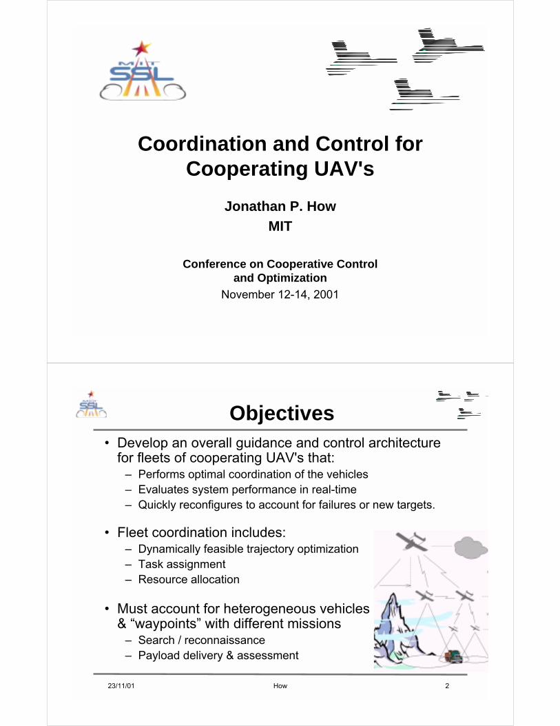
Objectives• Develop an overall guidance and control architecture

for fleets of cooperating UAV's that:– Performs optimal coordination of the vehicles – Evaluates system performance in real-time– Quickly reconfigures to account for failures or new targets.

• Fleet coordination includes:– Dynamically feasible trajectory optimization– Task assignment– Resource allocation

• Must account for heterogeneous vehicles & “waypoints” with different missions

– Search / reconnaissance– Payload delivery & assessment

23/11/01 How 3

Problem Statement• Vehicles

• Waypoints

• Obstacles

• Capabilities

• Optimize assignments & trajectories to minimizetime to complete overall mission

• Paper presents several solution algorithms.– Enable centralized and distributed coordination architectures

23/11/01 How 4

Encoding Problem Data• Collect assignment and trajectory optimization

problem data in matrix form• Initial states

• Dynamics

• Obstacles

• Targets

• Capabilities

• Time dependencies

M

M

iVmax

ΩM

M

imax

MMMM

MMMM

iiiiyxyx maxmaxminmin

M

M

M

M

jj TT yx

=

otherwise0point can visit vehicle1 jiKK iwiw

OLN

M

M

NLO

ij TT ≥

MMMM

MMMM

ii yxii vvyx

23/11/01 How 5

Basic Approach (MILP)• Approach: Mixed-Integer Linear Programming

– Extension of linear programming (LP) in which some variables take only integer values (0,1)

– Used to include logical statements in LP

• Benefits:– Can include high-level planning decisions directly in

trajectory optimization • Many path-planning problems can be written in MILP format• Directly includes avoidance conditions

– Software available to solve MILP problems – AMPL, CPLEX• Gives direct route to optimal solutions

⇒⇒⇒⇒ Can handle very general fleet guidance problems

• Issues:– Large, centralized computation– All models and constraints must be linearized

23/11/01 How 6

MILP Formulation• Assume linear model of UAV dynamics

– Point mass– Constant altitude ⇒ 2-D problem– Limited speed & force

⇒ Restricted turn rate

• Design maneuvers to give shortest flight time - penalize flight time

• Observation:– Minimum time solution favors max speed– Maximum speed ! turns at the rate limit– Sharper turns still permitted, must check.

max

maxmax

max

max

max

mVfVV

mVfffVV

≤Ω⇒=

≤Ω

≤≤

23/11/01 How 7

Magnitude Limits• Limited speed, force

• Exact constraint form is circle in vector space

– Nonlinear

• Approximate with Nlinear constraints

• Forms N-sided polygon in vector space

maxmax fV ≤≤+=fv

BfAxx&

N=4

N=6

N=8

Max. Error30%

N=4 N=12

23/11/01 How 8

Waypoint Visit Constraints• Logic & implementation

– Choose assignments and ordering consistent with capabilities matrix

• Waypoint must be visited by a capable vehicle– Gray squares

• Each waypoint must be visited exactly once– One in each row

• Binary variable vipw– v = 1 if vehicle p visits

target w at time i

( )( )

L

ipwTip

ipwTip

vMxx

vMxx

w

w

−−≥

−+≤

1

1

1, =∀ ∑∑i p

ipwiwvKw

23/11/01 How 9

Timing Constraints• Vehicle p visits target w at time TVpw

– Zero if vehicle does not visit that waypoint

• Vehicle p finishes at time TFp

• Mission completed at time TC

• Can use this information to include timing dependencies on the waypoint visitation.

∑ ⋅=∀∀i

ipwpw viTVpw ,,

pwp TVTFw ≥∀ ,

pTFTCp ≥∀ ,

23/11/01 How 10

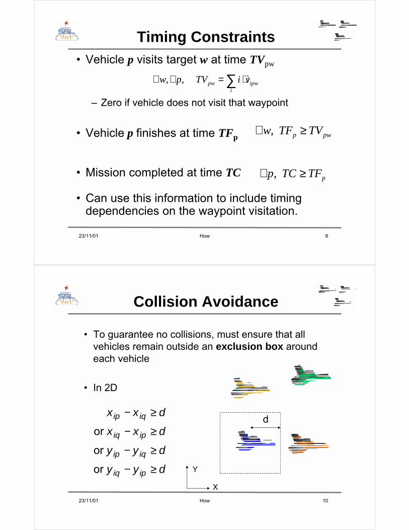
Collision Avoidance

• To guarantee no collisions, must ensure that all vehicles remain outside an exclusion box around each vehicle

• In 2D

x x dx x d

y y dy y d

ip iq

iq ip

ip iq

iq ip

− ≥

− ≥

− ≥

− ≥

or or or

X

Y

d

23/11/01 How 11

x x d Mb

x x d Mb

y y d Mb

y y d Mb

b

ip iq ipq

iq ip ipq

ip iq ipq

iq ip ipq

ipqkk

− ≥ −

− ≥ −

− ≥ −

− ≥ −

≤=

∑

1

2

3

4

1

43

and and and

and

Collision Avoidance as MILP• Convert ‘OR’ group to

‘AND’ group using binary variables

• bipqk either 0 or 1– b = 0 : constraint stands– b = 1 : relaxed

• M very large constant

• Schouwenaars et al. (ECC01)

Ensures at least 1 ‘or’ constraint holds

23/11/01 How 12

Optimization Objective

• Minimize overall completion time TC• Small α,β ensure unique solution exists

– Smooth trajectories from discretized limits• Subject to:

– Dynamics model– Visiting logic– Timing – Collision avoidance

∑∑ ++

pi

ipp

p

TCTFTV

TFTC,,,,

,,,)(min f

vbfxβα

23/11/01 How 13

Aircraft Model Validation

• Remains near max speed

• Single aircraft• A → B avoiding obstacles

–Blue: high turn rate–Red: low turn rate–Same speed

• Obeys turn rate limit ‘Turn-straight-turn’

AB

V ΩΩΩΩ

23/11/01 How 14

• Vehicle cannot visit target A

• Completion in 22 steps

Assignment Validation• Effect of Constraints

• 2 vehicles• 4 targets• All capabilities• Completion in 18 steps

A

23/11/01 How 15

• Add further constraints

• Target B must be visited before C

• Vehicle moves slowly• Completion in 27 steps

Assignment Validation II

B

C

• Added obstacle• Completion in 30

steps

B

C AA

23/11/01 How 16

Approximate Calculation Procedure

Compute all possible permutations & downselect

Find vehicle’s lowest cost paths to perform each feasible permutation

Optimal waypoint assignment

Calculate vehicle trajectories to visit waypoints in optimal order

Collision avoidance

Can be distributed

Centralized

Can bedistributed

Centralized

Centralized

23/11/01 How 17

Distributed Calculation

Compute all possible permutations & downselect

Optimal waypoint assignment

Collision avoidance

CostCalc #1

CostCalc #2

CostCalc #n-1

CostCalc #n

Trajectorydesign #1

Trajectorydesign #2

Trajectorydesign #n-1

Trajectorydesign #n

…

…

23/11/01 How 18

• Computationally efficient algorithm for finding costs

•Visibility graph: Which pairs of nodes can be connected without penetrating obstacles?

•Shortest paths: What are shortest paths between all pairs of waypoints?

Computing Cost Data• Assignment requires cost for all possible scenarios.

– With m waypoints and n vehicles, n (mP1 + mP2 + … + mPm) distinct sequences of starting points and waypoints.

• Computing cost values is the computationally demanding part of the assignment problem.

Obstacle fieldVisibility graphShortest paths between waypoints

23/11/01 How 19

Shortest paths between combination of 3 waypointsShortest Path for Vehicle 1

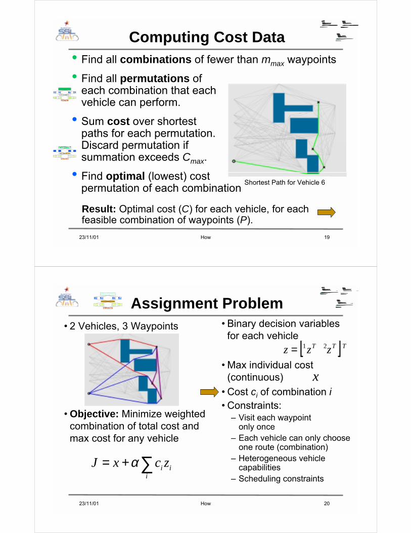
Computing Cost Data• Find all combinations of fewer than mmax waypoints

• Find all permutations of each combination that eachvehicle can perform.

• Sum cost over shortest paths for each permutation. Discard permutation if summation exceeds Cmax.

• Find optimal (lowest) cost permutation of each combination.

Result: Optimal cost (C) for each vehicle, for each feasible combination of waypoints (P).

Shortest Path for Vehicle 6

23/11/01 How 20

Assignment Problem• 2 Vehicles, 3 Waypoints

• Objective: Minimize weighted combination of total cost and max cost for any vehicle

• Binary decision variables for each vehicle

• Max individual cost (continuous)

• Cost ci of combination i• Constraints:

– Visit each waypoint only once

– Each vehicle can only choose one route (combination)

– Heterogeneous vehicle capabilities

– Scheduling constraints∑+=

iii zcxJ α

[ ] 21 TTT zzz =

x

23/11/01 How 21

(2) Visit waypoint only once

(3) Max cost ≥ max individual cost

Assignment Problem

=

101011

101111

100010001

L

L

L

L

L

L

P

Veh 1 n Combinations

Veh 2 m Comb’s

s WP'3,2,1 1 =∀=∑+

izPmn

jjij

sVeh' 2,1 =∀≤∑+

ixzCmn

jjij

• Combination matrix Pij

– 1 if waypoint i visited in combination j

– 0 if not• Cost matrix Cij

–Cost for vehicle i to perform combination j

–0 if vehicle i cannot execute combination j

" WP 1" WP 2" WP 3

=

m

,n,

cccc

C,21,2

111 0

00

0 L

L

L

L " Veh 1" Veh 2

11 =∑n

jjz 12 =∑

m

jjz

• Constraints(1) Choose only 1 combination

23/11/01 How 22

Trajectory Design• Assignment known, but still need trajectory

commands for vehicles⇒⇒⇒⇒ Use MILP to design feasible paths for vehicle

dynamics

• Design paths to prevent collisions– Could solve as centralized, fixed target MILP– Collisions unlikely in sparse problems⇒⇒⇒⇒ Distribute trajectory planning and check results– Redesign only those paths which collide

23/11/01 How 23

Solution Comparison

Optimal solution with approximate costs

Globally optimal solution with full MILP formulation

23/11/01 How 24

Larger Problem

23/11/01 How 25

Got MILP?• MILP can be used to solve many problems associated

with vehicle path-planning and fleet management

– Gives the global optimal solution subject to the linearity assumptions

– Centralized calculation

• Cost calculations for the assignment problem are most computational intensive part

– Developed techniques to approximate the costs calculation and distribute cost calculations.

• Algorithms can be used to support centralized and decentralized coordination architectures

– Further analysis required to investigate communication and computational trade-offs