coordinate transformations for … transforms in...coordinate transformations for cadastral...
TRANSCRIPT
COORDINATE TRANSFORMATIONS
FOR
CADASTRAL SURVEYING
R. E. Deakin
School of Mathematical and Geospatial Sciences, RMIT University
email: [email protected]
March 2007
ABSTRACT
1
yt
A two-dimensional (2D) conformal transformation, (that preserves shape and hence
angles), is a useful tool for practicing cadastral surveyors. It can be used as an aid to
re-establishment where occupation boundary corners of allotments, surveyed in the
field on an arbitrary survey coordinate system, can be transformed to the cadastral
title coordinate system and occupation/title comparisons made. The transformation
process consists of two parts. The first part is the determination of the
transformation parameters; scale s, rotation θ and translations, . This
requires a minimum of two control points having coordinates in both the title and
survey coordinate system. If there are three or more control points, then the
transformation parameters are determined by a least squares process and a weighting
scheme can be employed. The second part is to use the transformation parameters
(determined from the control points) to transform the other surveyed points onto the
title system. This paper sets out the necessary theory of 2D conformal
transformations and the determination of transformation parameters using least
squares. In addition, weighting schemes are discussed as well as transformations that
preserve scale (i.e., a scale ).
and xt
1s =
INTRODUCTION
Conformal coordinate transformations, are widely used in the surveying profession.
For instance, in geodesy, 3D conformal transformations can be used to convert
coordinates related to the Australian Geodetic Datum (AGD66, AGD84) to the

Geocentric Datum of Australia (GDA94), in engineering surveying they form part of
monitoring and control systems used in large projects such as the construction of
elevated freeways and tunnels (Deakin 1998), and in photogrammetry they are used
in the orientation (interior and exterior) of aerial digital images. In 2D form,
transformations are used in cadastral survey re-establishments (Bebb 1981, Sprott
1983 and Bird 1984), matching digitized cadastral maps (Shmutter and Doytsher
1991) and "sewing together" the edges of strips of digital images (Bellman, Deakin
and Rollings 1992).
2
t Nt
In general, the effect of a 2D transformation on a polygon (a plane multi-sided figure)
will vary from a simple change of location and orientation (with no change in shape
or size) to a uniform change in scale (no change in shape) and finally to changes of
shape and size of different degrees of nonlinearity (Mikhail 1976). The most common
transformations in surveying applications, and the only type dealt with in this paper,
are conformal, i.e., transformations that preserve angles and thus the shape of
objects. Theory and applications of other coordinate transformations, such as affine,
polynomial, projective etc. can be found in Mikhail (1976) and Moffitt and Mikhail
(1980). In the theory that follows, transformations are expressed in the form of
equations linking coordinates in one system with coordinates in another system and
these equations contain rotation angles (usually denoted by θ ), as well as scale s and
translations (or ) where the subscripts relate to the coordinate
system axes labels, x,y; E,N; u,v; etc. The idea of rotation is important and as we
will see there are several different types of rotations, i.e., an object can have an
and x yt and Et
actual rotation where it is rotated about a point; or an apparent rotation where its
coordinates change because the coordinate axes are rotated; and these rotations can
be clockwise or anticlockwise. In this paper we will only be considering apparent
rotations caused by anticlockwise rotation of coordinate axes and to clarify these
issues some rules and diagrams are helpful.
In general we consider points in space as being connected to the origin O of a 3D
right-handed rectangular coordinate system x,y,z. Such a system can be visualised as
the corner of a room where the intersection of two walls and the floor provide three
reference lines Ox, Oy and Oz, known as the x-, y- and z-axes that are (usually) at

right angles to one another. The x-z and y-z planes are the walls and the x-y plane is
the floor.
The three mutually perpendicular axes x, y
and z are related by the right-hand rule as
follows:
z
y
x
If the thumb, the forefinger and the second
finger of the right hand are placed
mutually at right angles then the thumb
points in the z-direction, the forefinger
points in the x-direction and the second
finger points in the y-direction.
z
x yθ
The axes x, y and z (in the cyclic order
xyz) are a right-handed system (or dextral
system) since a rotation from x towards y
advances a right-handed screw in the
direction of z. Similarly, a rotation from y
towards z advances a right-handed screw
in the direction of x and so on. The
diagram on the left shows the right-hand-
screw rule for the positive directions of
rotations and axes of a right-handed
rectangular coordinate system.
These rotations are considered positive anticlockwise when
looking along the axis towards the origin; the positive sense
of rotation being determined by the right-hand-grip rule
where an imaginary right hand grips the axis with the thumb
pointing in the positive direction of the axis and the natural
curl of the fingers indicating the positive direction of
rotation.
3
The right-handed coordinate system and positive anticlockwise rotations (given by
the right-hand-grip rule) are consistent with conventions used in mathematics and
physics and in mathematics, angles are measured positive anticlockwise from the x-
axis; a convention we also use in these notes. As surveyors, we deal almost
exclusively with angular quantities (bearing, azimuths, directions, etc) considered as
positive clockwise and usually measured from north (or the y-axis in the x-y system
or the v-axis in the u-v system) and this surveying convention of positive clockwise
rotation from north could be described by a left-hand-grip rule but we do not usually
do this.
CONFORMAL TRANSFORMATIONS IN TWO-DIMENSIONAL (2D) SPACE
In 2D conformal transformations all points lie in a plane and such points are
considered to have only x,y (or u,v) coordinates, i.e., they lie in the x-y (or u-v) plane
with a z-value = 0 (or w-value = 0). In these notes it is assumed that 2D conformal
transformations are transformations from one rectangular coordinate system (u,v)
which we could call the survey system to another rectangular system (x,y) that we
could call the title system. Both of these coordinate systems could be thought of as
arbitrary and it is immaterial where the origins of both systems lie. In addition,
unless stated otherwise, a rotation is an angle considered to be positive in an
anticlockwise direction as determined by the right-hand-grip rule and rotations of
polygons (or objects) are apparent, since we are considering rotations of coordinate
axes rather than actual rotations of polygons about a centre – more about this later.
Also, transformation equations are conveniently expressed using matrix notation and
a rotation matrix R (whose elements are functions of the rotation angle θ ) is a
component of any conformal transformation equation. Rotation matrices are
orthogonal, which is a very useful property, and there is an explanation of this
property in the following sections.
The general conformal transformation formula are developed in a simple way. First,
by considering transformations involving rotation only; then, involving both scale and
rotation. And finally, the general case, involving scale, rotation and translations.
We then show that this general conformal transformation (combining scale, rotation,
translation) is the same as that obtained by using the mathematical principles of
conformal mapping developed by C. F. Gauss.
4

Conformal Transformation involving Rotation only
u,v coordinates (survey system) are transformed to x,y (title system) coordinates by
considering a rotation of the u,v coordinate axes through a positive anticlockwise
angle θ . The transformation equations can be expressed in the following way
(1) cos sin
sin cos
x u v
y u v
θ θ
θ θ
= +
= − +
or in matrix notation
cos sin
sin cos
x uy
θ θ
θ θ v⎡ ⎤⎡ ⎤ ⎡ ⎤⎢ ⎥⎢ ⎥ ⎢ ⎥= ⎢ ⎥⎢ ⎥ ⎢ ⎥−⎣ ⎦ ⎣ ⎦⎢ ⎥⎣ ⎦
(2)
As an example consider the polygon ABCD whose u,v coordinates are rotated by a
positive anticlockwise angle . Figure 1 shows the initial location of the
polygon in the u,v survey system and Figure 2 shows its transformed (rotated)
location in the x,y title system.
30θ =
Point
100.000 250.000
200.000 423.205
286.602 373.205
157.735 150.000
u v
A
B
C
D
u
v
A
B
C
D
x
y
Figure 1 Polygon ABCD with u,v coordinates in metres
5

Point
211.603 166.506
384.808 266.506
434.807 179.904
211.603 51.036
x y
A
B
C
D
x
y
A
B
C
D
Figure 2 Rotated polygon ABCD with x,y coordinates in metres
Comparing Figures 1 and 2 it appears that the size and shape of the polygon ABCD
has not changed but its orientation with respect to the coordinate axes has. This can
be verified by considering the dimensions (bearings and distances) of the polygon
ABCD derived from the two coordinate sets.
Line Bearing Distance
30 00 200.000
120 00 100.000
210 00 257.735
330 00 115.470
AB
BC
CD
DA
′
′
′
′
Line Bearing Distance
60 00 200.000
150 00 100.000
240 00 257.735
0 00 115.470
AB
BC
CD
DA
′
′
′
′
Polygon dimensions in the u,v system Polygon dimensions in the x,y system
This example demonstrates that a rotation of the coordinate axes causes an apparent
rotation, in an opposite direction, of any polygon defined within the coordinate
system. The size and shape of the polygon does not change.
6

Equation (1) and its matrix equivalent (2) can be obtained by considering Figure 3.
u
v
y
xv
u •P
θ
v sin θ
v cos θ
u sin θ
u cos θ
Figure 3 x,y coordinates of P as functions of u,v coordinates and rotation θ
Rotation matrices
Equation (2) can be expressed as
cos sin
sin cos
x uy v
θ θ
θ θ
uv
⎡ ⎤⎡ ⎤ ⎡ ⎤ ⎡ ⎤⎢ ⎥⎢ ⎥ ⎢ ⎥ ⎢ ⎥= ⎢ ⎥⎢ ⎥ ⎢ ⎥ ⎢ ⎥−⎣ ⎦ ⎣ ⎦ ⎣ ⎦=
⎢ ⎥⎣ ⎦R (3)
where is known as a rotation matrix. Rotation matrices are
orthogonal, i.e., the sum of squares of the elements of any row or column is equal to
unity and an orthogonal matrix has the unique property that its inverse is equal to
its transpose, i.e., . This useful property allows us to write the
transformation from x,y coordinates to u,v coordinates as follows.
cos sin
sin cos
θ θ
θ θ
⎡ ⎤⎢= ⎢−⎢ ⎥⎣ ⎦
R ⎥⎥
1 T− =R R
1 1
T
x uy v
x uy v
x uy v
− −
⎡ ⎤ ⎡ ⎤⎢ ⎥ ⎢ ⎥=⎢ ⎥ ⎢ ⎥⎣ ⎦ ⎣ ⎦⎡ ⎤ ⎡ ⎤⎢ ⎥ ⎢= ⎥⎢ ⎥ ⎢ ⎥⎣ ⎦ ⎣⎡ ⎤ ⎡ ⎤⎢ ⎥ ⎢ ⎥=⎢ ⎥ ⎢ ⎥
⎦
⎣ ⎦ ⎣ ⎦
R
R R R
R I
and rearranging gives
cos sin
sin cosT
u xv y
θ θ
θ θ
xy
⎡ ⎤−⎡ ⎤ ⎡ ⎤ ⎡ ⎤⎢ ⎥⎢ ⎥ ⎢ ⎥ ⎢ ⎥= = ⎢ ⎥⎢ ⎥ ⎢ ⎥ ⎢ ⎥⎣ ⎦ ⎣ ⎦ ⎣ ⎦⎢ ⎥⎣ ⎦R (4)
7

We could write (4) as
8
xy
cos sin
sin cos
u xv y
θ θ
θ θ∗
⎡ ⎤−⎡ ⎤ ⎡ ⎤ ⎡ ⎤⎢ ⎥⎢ ⎥ ⎢ ⎥ ⎢ ⎥= =⎢ ⎥⎢ ⎥ ⎢ ⎥ ⎢ ⎥⎣ ⎦ ⎣ ⎦ ⎣ ⎦⎢ ⎥⎣ ⎦R
which in words means: the x,y coordinates are transformed (rotated) to u,v
coordinates. Equation (3) on the other hand means: the u,v coordinates are
transformed (rotated) to x,y coordinates and it is interesting to note that R and
are in fact the same rotation matrix except in the former, θ is positive anticlockwise
and in the latter θ is positive clockwise. Note that and
.
∗R
sin( ) sinθ θ− =−cos( ) cosθ θ− =
Orthogonal Matrices
Orthogonal matrices are extremely useful since their inverse is equal to their
transpose. Rotation matrices R are orthogonal, hence . A proof of this can
be found in Allan (1997) and is repeated here.
1 T− =R R
Consider the effect of a rotation on the coordinates x of a point P, expressed as
=X Rx
x
X is the transformed (or rotated) coordinates and R is the rotation matrix.
Multiplying both sides of the equation by the inverse of R gives
1 1− −=R X R Rx
but from matrix algebra and so 1− =R R I =Ix x
1− =R X x
or 1−=x R X
The length (actually squared length) of the line from the origin to the original
position of point P is given by and the length from the origin to the new
(rotated) position is given by . This length does not change due to rotation, i.e.,
it is invariant under rotation. Hence
Tx xTX X
T T=x x X X
but =X R
so ( )TT
T T
=
=
x x Rx Rx
x R Rx

For this result to be possible
T =R R I
but 1− =R R I
Therefore
1T −=R R
Thus the inverse of a rotation matrix is equal to its transpose.
Rotation of Axes versus Rotation of Object
In these notes it is assumed that a rotation angle is a positive anticlockwise angle as
determined by the right-hand-grip rule and that "apparent" rotations of objects
(polygons) are caused by a rotation of the coordinate axes. This is not the only way
that an object can be rotated.
x
y
·
·
θ
φ P
P'
o
d
d
Consider Figure 4 where P with coordinates x,y moves to
P' with coordinates x',y' by a positive anticlockwise
rotation φ . The coordinates of P' are
(5) ( ) (
( ) (
cos cos cos sin sin
sin sin cos cos sin
x d d
y d d
θ φ θ φ θ φ
θ φ θ φ θ φ
′= + = −
′= + = +
)
)
θ=
Figure 4
The coordinates of P are and y d which can be substituted into
(5) to give
cosx d θ= sin
or in matrix form cos sin
cos sin
x x y
y y x
φ φ
φ φ
′= −
′= +
cos sin
sin cos
x xyy
φ φ
φ φ
xy
⎡ ⎤′ ⎡ ⎤− ⎡ ⎤ ⎡ ⎤⎢ ⎥ ⎢ ⎥ ⎢ ⎥ ⎢ ⎥= =⎢ ⎥ ⎢ ⎥ ⎢ ⎥ ⎢ ⎥′⎢ ⎥ ⎣ ⎦ ⎣ ⎦⎢ ⎥⎣ ⎦⎣ ⎦R (6)
Where R is a rotation matrix and the rotation angle φ is a "right-handed" rotation.
Inspection of equations (3) and (6) shows that R is not the same form as R, in fact
it is identical in form to . TRThe rotation matrix R causes an apparent rotation of the object by rotation of the
coordinate axes whilst the rotation matrix R rotates the object itself. Both R and
R are "right-hand" rotation matrices (one is the transpose of the other) and there is
often confusion amongst users of transformation software in defining the type of
9
rotation and the positive direction of rotation. You must be very careful in defining
rotation, i.e., you must state what is being rotated, either axes or object and what is
the positive direction of rotation. In these notes it is always assumed that the
coordinate axes are being rotated and the rotations are always positive anticlockwise
as defined by the right-hand-grip rule.
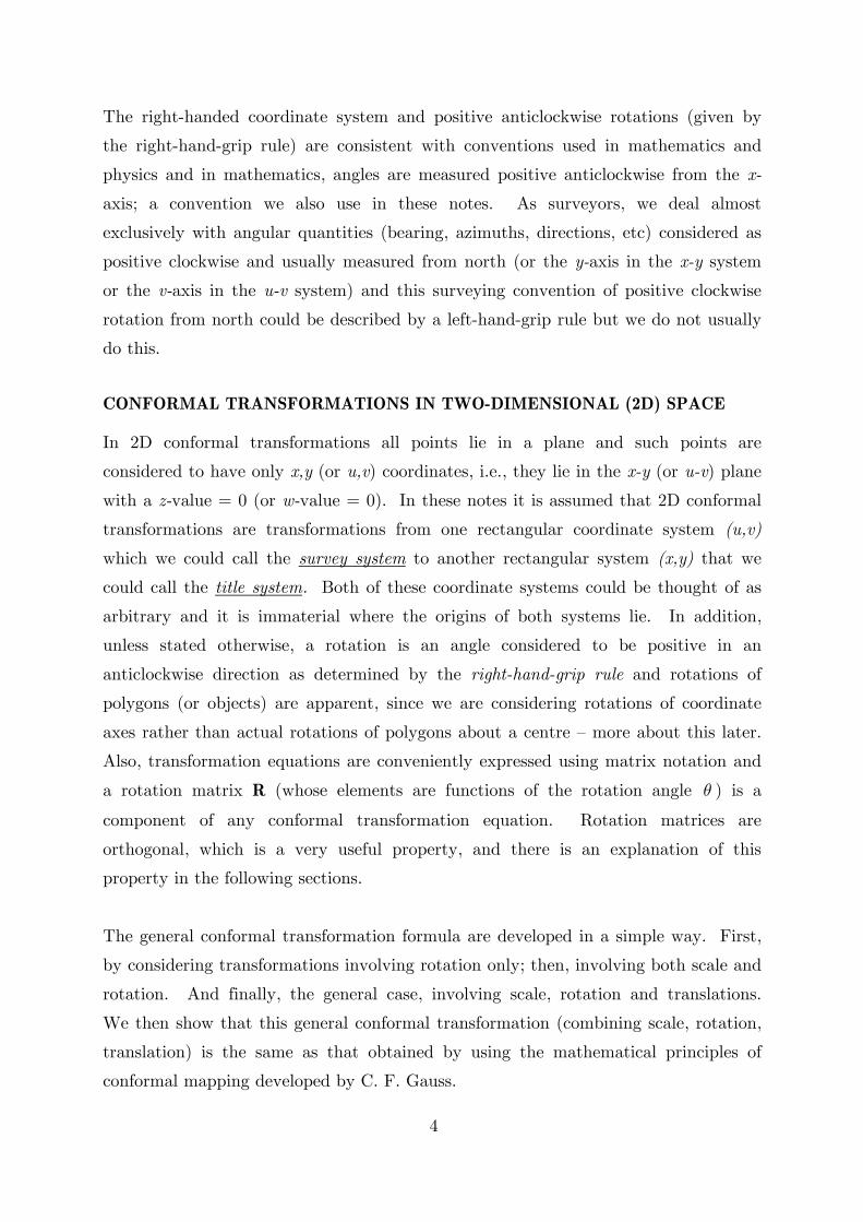
Conformal Transformation involving Rotation θ and a Scale change s
u,v coordinates (survey system) are transformed to x,y coordinates (title system) by
considering a rotation of the u,v coordinate axes through a positive anticlockwise
angle and a scaling of the u,v coordinates by a factor s. The transformation
equations can be expressed in the following way
θ
( ) ( )
( ) (
cos sin
sin cos
x s u s
y s u s
θ θ
θ θ
= +
=− + )
v
v
v
(7)
or in matrix notation
cos sin
sin cos
x usy
θ θ
θ θ
⎡ ⎤⎡ ⎤ ⎡ ⎤⎢ ⎥⎢ ⎥ ⎢ ⎥= ⎢ ⎥⎢ ⎥ ⎢ ⎥−⎣ ⎦ ⎣ ⎦⎢ ⎥⎣ ⎦ (8)
Often, the coefficients of u and v in (7) are written as and
giving
cosa s θ= sinb s θ=
x a by b a
uv
⎡ ⎤⎡ ⎤ ⎡ ⎤⎢ ⎥⎢ ⎥ = ⎢ ⎥⎢ ⎥⎢ ⎥ − ⎢ ⎥⎣ ⎦ ⎣ ⎦⎢ ⎥⎣ ⎦ (9)
and the scale factor s and the rotation angle θ are given by
2 2
1tan
s a b
ba
θ −
= +
⎛ ⎞⎟⎜= ⎟⎜ ⎟⎜⎝ ⎠
(10)
10

As an example consider the polygon ABCD whose u,v coordinates (survey system)
are rotated by a positive anticlockwise angle and scaled by a factor .
Figure 1 shows the initial location of the polygon in the u,v system and Figure 5
shows its transformed (rotated and scaled) location in the x,y system (title system).
30θ = 0.6s =
Point
126.962 99.904
230.885 159.904
260.884 107.942
126.962 30.622
x y
A
B
C
D
x
y
AB
C
D
Figure 5 Rotated and scaled polygon ABCD with x,y coordinates in metres
Comparing Figures 1 and 5 it appears that the shape of the polygon ABCD has not
changed but its size and orientation with respect to the coordinate axes has. This
can be verified by considering the dimensions (bearings and distances) and area of the
polygon ABCD derived from the two coordinate sets.
2
Line Bearing Distance
30 00 200.000
120 00 100.000
210 00 257.735
330 00 115.470
Area=22,886.75m
AB
BC
CD
DA
′
′
′
′
2
Line Bearing Distance
60 00 120.000
150 00 60.000
240 00 154.641
0 00 69.282
Area=8,239.23m
AB
BC
CD
DA
′
′
′
′
Polygon dimensions in the u,v system Polygon dimensions in the x,y system
Inspection of the two sets of dimensions reveals that bearings have been rotated by
an angle and distances scaled by a factor . 30θ = 0.6s = Note that the shape of
the polygon is unchanged but the area of the transformed figure has been reduced by
a factor of . 2s
11

Conformal Transformation with Rotation , Scale change s and Translations θ ,x yt t
u,v coordinates (survey system) are first transformed to coordinates by
considering a rotation of the u,v coordinate axes through a positive anticlockwise
angle θ and a scaling of the u,v coordinates by a factor s. The coordinates are
then transformed into x,y coordinates (title system) by the addition of translations
and t .
,x y′ ′
,x y′ ′
xt
y
The transformation equations can be expressed in the following way
( ) ( )
( ) ( )
cos sin
sin cosx
y
x s u s v
y s u s v
θ θ
θ θ
= +
=− + +
t
t
+
v
(11)
or in matrix notation
cos sin
sin cosx
y
x u tsy t
θ θ
θ θ
⎡ ⎤ ⎡ ⎤⎡ ⎤ ⎡ ⎤⎢ ⎥ ⎢ ⎥⎢ ⎥ ⎢ ⎥= ⎢ ⎥ + ⎢ ⎥⎢ ⎥ ⎢ ⎥−⎣ ⎦ ⎣ ⎦⎢ ⎥ ⎣ ⎦⎣ ⎦ (12)
or x
y
x u tsy v t
⎡ ⎤⎡ ⎤ ⎡ ⎤ ⎢ ⎥⎢ ⎥ ⎢ ⎥= + ⎢ ⎥⎢ ⎥ ⎢ ⎥⎣ ⎦ ⎣ ⎦ ⎣ ⎦R
Similarly to before writing and gives cosa s θ= sinb s θ=
x
y
x a b u ty v tb a
⎡ ⎤ ⎡ ⎤⎡ ⎤ ⎡ ⎤⎢ ⎥ ⎢ ⎥⎢ ⎥ ⎢ ⎥= ⎢ ⎥ + ⎢ ⎥⎢ ⎥ ⎢ ⎥−⎣ ⎦ ⎣ ⎦⎢ ⎥ ⎣ ⎦⎣ ⎦ (13)
This transformation is referred to by several names
(i) Four-parameter transformation, the four parameters being , , , ,x ya b t t
(ii) 2D Linear Conformal transformation,
(iii) Similarity transformation and
(iv) Helmert's transformation, after the German geodesist F.R. Helmert (1843-
1917).
Note that "linear" is sometimes used in the description of a conformal transformation
to differentiate it from a polynomial conformal transformation. Polynomial conformal
transformations are rarely used so the distinction will not be used hereafter.
12

The 2D (linear) conformal transformation equations may be derived by considering
Figure 6. The coordinates are obtained by rotating and scaling the u,v
coordinates; and then the x,y coordinates obtained by adding the translations and
to the coordinates. This two-step process is given by the equations:
,x y′ ′
xt
yt ,x y′ ′
cos sin
sin cos
x
y
x us vy
x x ty ty
θ θ
θ θ
⎡ ⎤′ ⎡ ⎤ ⎡ ⎤⎢ ⎥ ⎢ ⎥ ⎢ ⎥=⎢ ⎥ ⎢ ⎥ ⎢ ⎥−′⎢ ⎥ ⎣ ⎦⎢ ⎥⎣ ⎦⎣ ⎦⎡ ⎤′ ⎡ ⎤⎡ ⎤ ⎢ ⎥ ⎢ ⎥⎢ ⎥ = +⎢ ⎥ ⎢ ⎥⎢ ⎥ ′⎢ ⎥⎣ ⎦ ⎣ ⎦⎣ ⎦
u
vy
x
v
u· P
y'
x'
v sin θ
u cos θ
v co
s θ
u sin θ
θt
t
y
x
Figure 6. Schematic diagram of rotated and translated axes
Note that in Figure 6, and are both positive quantities, but in general, they
may be positive or negative. xt yt
13

As an example of a 2D Conformal transformation, consider the polygon ABCD whose
u,v coordinates are rotated by a positive anticlockwise angle , scaled by a
factor and translated by and Figure 1 shows
the initial location of the polygon in the u,v survey system and Figure 7 shows its
transformed (rotated, scaled and translated) location in the x,y title system.
30θ =0.6s = 50.000mxt = 150.000myt =
Point
176.962 249.904
280.885 309.904
310.884 257.942
176.962 180.622
x y
A
B
C
D
x
y
A
B
C
D
Figure 7 Rotated, scaled and translated polygon ABCD with x,y coordinates in metres
Comparing Figures 1 and 7 it appears that the shape of the polygon ABCD has not
changed but its area and orientation with respect to the coordinate axes has. This
can be verified by considering the dimensions (bearings and distances) and area of the
polygon ABCD derived from the two coordinate sets.
2
Line Bearing Distance
30 00 200.000
120 00 100.000
210 00 257.735
330 00 115.470
Area=22,886.75m
AB
BC
CD
DA
′
′
′
′
2
Line Bearing Distance
60 00 120.000
150 00 60.000
240 00 154.641
0 00 69.282
Area=8,239.23m
AB
BC
CD
DA
′
′
′
′
Polygon dimensions in the u,v system Polygon dimensions in the x,y system
Inspection of the two sets of dimensions reveals that bearings and distances of the
polygon in the u,v system have been has been rotated by an angle and scaled
by a factor .
30θ =0.6s = Note that the shape of the polygon is unchanged but the area of
the transformed figure has been reduced by a factor of . Comparison with the
previous transformation demonstrates that
2s
translation has no effect on the area,
shape and orientation of a polygon.
14

2D Conformal Transformation derived using conformal mapping theorems
C.F. Gauss (1777-1855) showed that the necessary and sufficient condition for a
conformal transformation from the ellipsoid to the map plane is given by the complex
expression (Lauf 1983)
15
))
(14) (y i x f iχ ω+ = +
where the function is analytic, containing isometric parameters
(isometric latitude) and ω (longitude) and in this equation the x-axis is east-west
and the y-axis is north-south. i is the imaginary number (
(f iχ ω+ χ
2 1i = − ). It should be
noted here that isometric means of equal measure, and on the surface of the ellipsoid
(or sphere) latitude and longitude are not equal measures of length. This is obvious
if we consider a point near the pole where similar distances along a meridian and a
parallel of latitude will correspond to vastly different angular values of latitude and
longitude. Hence in conformal map projections, isometric latitude is determined to
ensure that angular changes correspond to linear changes.
A necessary condition for an analytic function is that it must satisfy the Cauchy-
Riemann equations
andy x yχ ω ω
∂ ∂ ∂ ∂= =−∂ ∂ ∂ ∂
xχ
)
(15)
Using this theorem, a conformal transformation from one plane rectangular
coordinate system u,v (isometric parameters) to another plane rectangular system x,y
(also isometric parameters) is given by the complex expression
(16) (y i x f v i u+ = +
A function ( )f v i u+ that satisfies the Cauchy-Riemann equations, is a complex
polynomial, hence (16) can be given as
( )( )0
n k
k kk
y i x a ib v i u=
+ = + +∑ (17)
Equation (17) can be expanded to the first power (k = 1) giving
0 1
0 0 1 1
20 0 1 1 1 1
( )( ) ( )( )y ix a ib v iu a ib v iu
a b i a v a ui b vi b ui
+ = + + + + +
= + + + + +

Equating real and imaginary parts (remembering that ) gives 2 1i =−
16
v
v (18)
0 1 1
0 1 1
x b a u b
y a b u a
= + +
= − +
or in matrix notation with translations and between the coordinate axes 0a 0b
1 1 0
01 1
x a b u by v ab a
⎡ ⎤ ⎡ ⎤⎡ ⎤ ⎡ ⎤⎢ ⎥ ⎢ ⎥⎢ ⎥ ⎢ ⎥= ⎢ ⎥ + ⎢ ⎥⎢ ⎥ ⎢ ⎥−⎣ ⎦ ⎣ ⎦⎢ ⎥ ⎣ ⎦⎣ ⎦ (19)
These equations are of similar form to equations (13) in the section headed
"Conformal Transformations with Rotation, Scale and Translations" and properly
describe a 2D Conformal transformation. Note that the elements of the leading
diagonal of the coefficient matrix (a rotation matrix multiplied by a scale factor) are
identical and the off-diagonal elements the same magnitude but opposite sign.
Equations (18) are essentially the same equations as in Jordan/Eggert/Kneissal (1963,
pp. 70-73) in the section headed "Das Helmertsche Verfahren (Helmertsche
Transformation)" (Helmert's Transformation) although as noted by Bervoets (1992)
in his bibliography, there is no reference to the original source. It is probable that
F.R. Helmert developed this conformal transformation in his masterpiece on geodesy,
Die mathematischen und physikalischen Theorem der höheren Geodäsie, (The
mathematics and physical theorems of higher geodesy) on which he worked from 1877
and published in two parts: vol. 1, Die mathematischen Theorem (1880) and vol. 2,
Die physikalischen Theorem (1884) [DSB 1972]. This probably accounts for the
common usage of the term Helmert transformation when describing a 2D Conformal
transformation.
The partial derivatives of (18) are
1 1 1, , andx x y ya b bu v u v
∂ ∂ ∂ ∂= = = − =∂ ∂ ∂ ∂ 1a
which satisfy the Cauchy-Riemann equations
andy x yv u u
∂ ∂ ∂ ∂= = −∂ ∂ ∂ ∂
xv
so verifying that the transformation is conformal.

17
SOLVING FOR CONFORMAL TRANSFORMATION PARAMETERS
Coordinate transformations, as used in practice, are models describing the assumed
mathematical relationships between points in two rectangular coordinate systems; in
these notes, the u,v (survey) and the x,y (title) systems. To determine the
parameters of any transformation, coordinates of points common to both systems
must be known. These points are known as control points or common points. The
number of common points required for the solution of transformation parameters
depends on the number of parameters in the transformation. In 2D transformations,
each common point gives rise to two equations, thus n common points will give 2n
equations. Therefore, if the four parameters of a 2D Conformal transformation are to
be determined, then a minimum of two common points are required to solve for the
parameters.
It is good measurement practice to determine coordinate transformation parameters
by using more than the minimum number of common points. This introduces
redundant equations into the solution for the parameters and the theory of least
squares is employed to calculate the best estimates. Parameters calculated in this
manner are usually more reliable and the least squares process allows precision
estimation of the parameters as well as an assessment (via residuals) of how well the
transformation model fits the common points. By using least squares, several types
of transformations can be "tested" on the common points to assess their suitability.
The solution for the transformation parameters involves the following steps
(i) Select the common points ensuring that there are sufficient to allow a redundant
set of equations.
(ii) Select the appropriate weight matrix W for the model.
(iii) Solve for the parameters (contained in the vector x) and residuals (contained in
the vector v).
(iv) Assess the suitability of the model by analysis of the parameters and residuals.

Mathematical model for solution of 2D Conformal Transformation Parameters
18
n
The 2D Conformal transformation, or the mathematical model, consisting of rotation,
scaling and translation is set out above [see equation (13)] and the transformation for
the common points is given in the form of observation equations
(20)
1, 2, 3, ,k = …
k
k
k x k x
k y k y
x v a b u ty v v tb a
⎡ ⎤ ⎡ ⎤⎡ ⎤ ⎡ ⎤ ⎡ ⎤⎢ ⎥ ⎢ ⎥⎢ ⎥ ⎢ ⎥ ⎢ ⎥+ = +⎢ ⎥ ⎢ ⎥⎢ ⎥ ⎢ ⎥ ⎢ ⎥−⎣ ⎦ ⎣ ⎦ ⎣ ⎦⎢ ⎥ ⎣ ⎦⎣ ⎦ (20)
where and are small unknown corrections or residuals simply added to the
equations to account for the assumed inconsistency in the model. We could think of
these residuals as consisting of two parts; one part associated with the u,v (survey)
system and the other associated with the transformed x,y (title) system; the
subscripts x and y attached to the residuals simply reflect the fact that they have
been added to the "transformed" side of the model.
kxvky
v
Re-arranging (20) so that all the "unknowns" are on to the left of the equals sign and
the observations are to the right gives
(21) k
k
x k k x
y k k y
v a u b v t x
v a v b u t y
− − − = −
− + − = −k
k
For n common points and unknown parameters, the partitioned matrix
representation of the 2n equations (21) is
4u =
1
2
3
1
2
3
1 1
2 2
3 3
1 1
2 2
3 3
1 0
1 0
1 0
1 0
0 1
0 1
0 1
0 1
n
n
x
x
xx
x n n
y
y
y
yn n
u vv au vv bu vv t
tv u vv v uv v uv v u
vv u
⎡− − − ⎤⎢ ⎥⎡ ⎤⎢ ⎥⎢ ⎥ − − −⎢ ⎥⎢ ⎥ ⎢ ⎥⎢ ⎥ − − −⎢ ⎥⎢ ⎥ ⎢ ⎥⎢ ⎥⎢ ⎥⎢ ⎥⎢ ⎥⎢ ⎥⎢ ⎥⎢ ⎥ − − −⎢ ⎥⎢ ⎥ ⎢ ⎥⎢ ⎥ + ⎢ ⎥− −⎢ ⎥⎢ ⎥⎢ ⎥⎢ ⎥⎢ ⎥ − −⎢ ⎥⎢ ⎥ ⎢ ⎥⎢ ⎥ − −⎢ ⎥⎢ ⎥⎢ ⎥⎢ ⎥⎢ ⎥⎢ ⎥⎢ ⎥⎢ ⎥ ⎢ ⎥⎢ ⎥⎣ ⎦ − −⎢ ⎥⎣ ⎦
1
2
3
1
2
3
y
n
n
xxx
xyyy
y
−⎡ ⎤⎡ ⎤ ⎢ ⎥⎢ ⎥ −⎢ ⎥⎢ ⎥ ⎢ ⎥⎢ ⎥ −⎢ ⎥⎢ ⎥ ⎢ ⎥⎢ ⎥ ⎢ ⎥⎢ ⎥ ⎢ ⎥⎢ ⎥⎣ ⎦ ⎢ ⎥−⎢ ⎥⎢ ⎥= −⎢ ⎥⎢ ⎥−⎢ ⎥⎢ ⎥−⎢ ⎥⎢ ⎥⎢ ⎥⎢ ⎥⎢ ⎥−⎢ ⎥⎣ ⎦
(22)

These equations are represented by the matrix equation
v Bx f+ = (23)
where
v is a (2n,1) column vector of residuals
B is a (2n,u) matrix of coefficients
x is a (u,1) vector of unknown parameters
f is a (2n,1) column vector of numeric terms (coordinates)
The normal equations for the least squares solution of parameters x and residuals v
are given in matrix form as
(24) ( )T =B WB x B WfT
or
(25) =Nx t
where
is the (u,u) symmetric coefficient matrix of the normal equations T=N B WB is the (u,1) vector of numeric terms of the normal equations T=t B Wf
1
2
1
2
0 0 0 0
0 0
0 0
0
0
0 0
n
n
w
w
w
w
w
w
⎡ ⎤⎢ ⎥⎢ ⎥⎢ ⎥⎢ ⎥⎢ ⎥⎢ ⎥⎢ ⎥⎢ ⎥= ⎢ ⎥⎢ ⎥⎢ ⎥⎢ ⎥⎢ ⎥⎢ ⎥⎢ ⎥⎢ ⎥⎢ ⎥⎣ ⎦
W
0
0
is the (2n,2n) diagonal weight matrix where the weights on the upper-left
diagonal are repeated on the lower-right diagonal. Weights are usually integer
values and high weights are associated with "strong" points and low weights
associated with "weak" points.
kw
19

The general form of the normal equations are =Nx t
( )
( )
( )
( )
2 2
11 1 1
2 2
11 1 1
11
1 1
0
0
symmetric
nn n n
k k k k kk k k k k k kkk k k
nn n n
k k k k kk k k k k k kkk k k
nnx
k kky kk
n n
k k kk k
w u x v yw u v w u w v
aw v x u yw u v w v w u b
tw xw t
w w y
== = =
== = =
==
= =
⎡⎡ ⎤ +⎢+⎢ ⎥⎢ ⎥⎢ ⎥ ⎡ ⎤⎢ ⎥ ⎢ ⎥ −⎢ ⎥+ − ⎢ ⎥⎢ ⎥ ⎢ ⎥⎢ ⎥ =⎢ ⎥⎢ ⎥ ⎢ ⎥⎢ ⎥ ⎢ ⎥⎢ ⎥ ⎢ ⎥⎣ ⎦⎢ ⎥⎢ ⎥⎢ ⎥⎢ ⎥⎣ ⎦ ⎣
∑∑ ∑ ∑
∑∑ ∑ ∑
∑∑
∑ ∑
⎤⎥
⎢ ⎥⎢ ⎥⎢ ⎥⎢ ⎥⎢ ⎥⎢ ⎥⎢ ⎥⎢ ⎥⎢ ⎥⎢ ⎥⎢ ⎥⎢ ⎥⎢ ⎥⎦
(26)
Centroidal coordinates
Computational savings can be made by reducing coordinates to a weighted centroid.
For the n common points, the coordinates of the weighted centroid in the x,y
system are
,c cx y
1 1 2 2 3 3 1
1 2 3
1
1 1 2 2 3 3 1
1 2 3
1
n
k kn n k
ncn
kk
n
k kn n k
ncn
kk
w xw x w x w x w xx
w w w w w
w yw y w y w y w yy
w w w w w
=
=
=
=
+ + + += =+ + + +
+ + + += =+ + + +
∑
∑
∑
∑
(27)
Note here that coordinates of the weighted centroid are just the weighted
arithmetic means of the coordinates of the n common points. Also, note that if all
points have the same weight then the coordinates of the centroid are
,c cx y
,c cx y
1 1,
n n
k kk k
c c
x yx y
n n= == =∑ ∑
Now, the centroidal coordinates of the n common points in the x,y system are then
1 1 1 1
2 2 2 2
3 3 3 3
c c
c c
c
n n c n n
x x x y y yx x x y y yx x x y y y
x x x y y y
= − = −= − = −= − = −
= − = −
c
c
(28)
20

Similar relationships can be written for centroidal coordinates in the u,v system. A
useful property of the centroidal coordinates of the n common points is that their
sums equal zero, i.e.,
1 1 1 1
0, 0, 0, 0n n n n
k k k k k k k kk k k k
w x w y w u w v= = = =
= = =∑ ∑ ∑ ∑ = (29)
Thus, replacing x,y and u,v coordinates with their centroidal counterparts ,x y and
,u v reduces the observation equations (20) to a centroidal form
k
k
xk
yk k
v a bx uvy b a
k
v⎡ ⎤⎡ ⎤ ⎡ ⎤⎡ ⎤ ⎢ ⎥⎢ ⎥ ⎢ ⎥⎢ ⎥+ = ⎢ ⎥⎢ ⎥ ⎢ ⎥⎢ ⎥ −⎣ ⎦ ⎢ ⎥⎣ ⎦ ⎣ ⎦⎣ ⎦
(30)
It should be noted here that translations and are both zero when centroidal
coordinates are used indicating that the centroids and are the same point. xt yt
,c cx y ,c cu v
For n common points and unknown parameters, the partitioned matrix
representation of the 2n observation equations resulting from the centroidal model
(30) is
2u =
1
2
3
1
2
3
11 1
22 2
33 3
11 1
22 2
33 3
n
n
x
x
x
x nn n
y
y
y
y nn n
v xu vv xu v av xu v b
v xu vv yv uv yv uv yv u
v yv u
−− −⎡ ⎤⎡ ⎤ ⎢ ⎥⎢ ⎥ ⎢ ⎥ −− −⎢ ⎥ ⎡ ⎤⎢ ⎥⎢ ⎥ ⎢ ⎥⎢ ⎥⎢ ⎥ −− − ⎢ ⎥⎢ ⎥⎢ ⎥ ⎣ ⎦⎢ ⎥⎢ ⎥ ⎢ ⎥⎢ ⎥ ⎢ ⎥⎢ ⎥ −− −⎢ ⎥⎢ ⎥ ⎢ ⎥⎢ ⎥ + −−⎢ ⎥⎢ ⎥ ⎢ ⎥⎢ ⎥ ⎢ ⎥ −−⎢ ⎥ ⎢ ⎥⎢ ⎥ ⎢ ⎥⎢ ⎥ −−⎢ ⎥⎢ ⎥ ⎢ ⎥⎢ ⎥ ⎢ ⎥⎢ ⎥ ⎢ ⎥⎢ ⎥ −−⎢ ⎥⎢ ⎥⎣ ⎦
=
⎣ ⎦
⎡ ⎤⎢ ⎥⎢ ⎥⎢ ⎥⎢ ⎥⎢ ⎥⎢ ⎥⎢ ⎥⎢ ⎥⎢ ⎥⎢ ⎥⎢ ⎥⎢ ⎥⎢ ⎥⎢ ⎥⎢ ⎥⎢ ⎥⎢ ⎥⎢ ⎥⎢ ⎥⎢ ⎥⎣ ⎦
(31)
These equations are represented by the matrix equation (23) and the normal
equations have the following simple form containing only three different numbers
( )
( )
( )
( )
2 2
1
2 2
1 1
0
0
n n
k k k k k k k kk k
n n
k k k k k k k kk k
w u v w u x v ya
bw u v w v x u y
=
= =
⎡ ⎤ ⎡+ +⎢ ⎥ ⎢⎡ ⎤⎢ ⎥ ⎢⎢ ⎥ =⎢ ⎥ ⎢⎢ ⎥⎢ ⎥ ⎢⎣ ⎦+ −⎢ ⎥ ⎢⎢ ⎥ ⎢⎣ ⎦ ⎣
∑ ∑
∑ ∑1=
⎤⎥⎥⎥⎥⎥⎥⎦
(32)
21

The solutions for the parameters a and b are
( )
( )1
2 2
1
n
k k k k kk
n
k k kk
w u x v ya
w u v=
=
+=
+
∑
∑ (33)
( )
( )1
2 2
1
n
k k k k kk
n
k k kk
w v x u yb
w u v=
=
−=
+
∑
∑ (34)
The translations and are obtained by re-arranging (13) and replacing x,y and
u,v with the coordinates of the centroid and giving xt yt
,c cx y ,c cu v
c cx
c cy
x a btyt b a
uv
⎡ ⎤⎡ ⎤ ⎡ ⎤ ⎡ ⎤⎢ ⎥⎢ ⎥ ⎢ ⎥= − ⎢ ⎥⎢ ⎥⎢ ⎥ ⎢ ⎥ − ⎢ ⎥⎣ ⎦ ⎣ ⎦⎢ ⎥⎣ ⎦ ⎣ ⎦ (35)
or (36) x c c
y c c
t x au bv
t y bu av
= − −
= + −c
c
After calculation of the parameters, T
x ya b t t⎡ ⎤= ⎢ ⎥⎣ ⎦x the residuals are calculated
using (31).
The least squares solution for the transformation parameters looks formidable, but it
really is very simple. The parameters for any 2D Conformal transformation can be
computed using a pocket calculator and this solution depends on forming only three
numbers from a system of centroidal coordinates. Alternatively, a simple computer
program spreadsheet (such as Excel) could be used.
In the following pages an example of a 2D Conformal transformation as an aid to
cadastral re-establishment will be discussed.
22

CONFORMAL TRANSFORMATION EXAMPLE
Figure 8 shows a Plan of Subdivision (LP48556) with distances in links (1 chain =
100 links = 66 feet) and bearings related to True North. The plan shows two
Reference Marks (RM's), one near the south-west corner of Lot 1 and the other near
the south-east corner of the 100 link wide access to Lot 2. The subdivision was
created and marked on the ground in the 1920's.
0° 0
0′
30° 0
0′
90° 00′
90° 00′
100
100
1000
3000
120° 00′ ROAD
520.1
1688.9
2250.52366
1575
.7
1578
2098
.1
RM
RM
210°
00′
210°
00′
10
101
2N
TRU
E
Distances in links
115.5
LP 48556
Figure 8 Plan of Subdivision LP48556
Figure 9 shows an Abstract of Fieldnotes of a recent survey conducted for the
purposes of boundary re-establishment prior to purchase of Lot 2, LP 48556. At the
time of survey only one of the RM's along the road was found and old pegs, thought
to be original, were found at the south-west and north-east corners of Lot 2. Most of
the fencing was fairly recent, probably replacing original fencing. The post at the
north-east corner of Lot 2, which is new, is very close to the old peg which may have
been disturbed when the new post was put in. The other old peg at the south-west
corner of Lot 2 appeared to be original and undisturbed.
23
ROAD
RM found
1
2
⊗
⊗
⊗
⊗
⊗
⊗∧
∧
∧
∧∧
∧
post
an
d
wire
post
an
d
wire
post and wire
post and wire
post & wire
post
an
d w
ire
p & w
p & w
p & w
p & w
N
00
00
0000
5.225
477.9
4 590° 00′
300° 00′
0°00
′
0°00
′
30° 0
0′
30° 0
0′
98° 26′
3 0 6° 0 1′
251°
56′
67° 42′
67° 1
6′
59° 07′
161° 37′
72° 37′ 2.730
2.605OP Fd.
108.115
420.415
3.935 5.745
OP F
d.5.8
60
199.
180600.450
332.460
15.4
0 0
1 7 .9 95
5.740
ABSTRACT OF FIELDNOTESDATUM A-B
Distances in metres
00
2.010
A
B
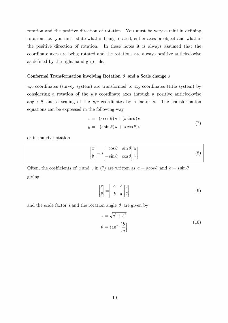
Figure 9 Abstract of Fieldnotes of survey of Lot 2, LP48556
The datum of the survey was the post A (south-west corner of Lot 1) and the RM B
found near the south-east corner of the road access to Lot 2. A traverse line offset
2.010 m (10 links) from the post at A and passing through the RM was adopted for
the bearing datum of 300° 00′
For this example we will perform a cadastral re-establishment using a 2D Conformal
transformation (scale, rotation and translations) with weights based on the RM and
the two old pegs of LP48556. In light of the information above, the RM will be given
a weight of 10, the old peg at the south-west corner of Lot 2 will be given a weight of
5 and the other old peg (north-east corner of Lot 2) will be given a weight of 1.
24

25
The parameters of the transformation (scale, rotation and translations) will be
determined and an inspection of residuals will give some indication as to the
"correctness" of the re-establishment.
For the purposes of computing the transformation parameters, two arbitrary
coordinate systems will be used. One system of coordinates, in metres, called TITLE
will have values of 5000.000 E and 5000.000 N for the RM near the south-east corner
of the road access to Lot 2. For the purpose of computing the TITLE coordinates
the original dimensions in links will be converted to metres where 1 chain = 100 links
= 66 feet, and 1 foot = 0.3048 metres (exactly) giving links × 0.201168 = metres.
The original dimensions of 1000 links, 3000 links and 1578 links will be converted to
metres (3 decimal places) and the other dimensions "computed to close" and noted to
4 decimal places. The road access frontage will be derived by computation after
converting the 100 link width to 20.117 metres. This computation process should
ensure that coordinates are mathematically correct to 3 decimal places.
The other system of coordinates, also in metres, and called SURVEY will have values
of 2000.000 E and 2000.000 N for the RM found. The traverse dimensions are
mathematically correct (to a millimetre) and should yield SURVEY coordinates of
traverse points and occupation correct to 3 decimal places.

0° 0
0′
30° 0
0′
90° 00′
90° 00′
100
100
1000
3000
120° 00′ ROAD
520.
1
1688.9
2250.52366
1575
.7
1578
2098
.1
RM
RM
210°
00′
210°
00′
10
10
1
2
NTR
UE
Distances in linksDistances in metres
115.5
5001.006 E5605.246 N
4641.1165330.333
4980.8895330.333
4588.8055239.727
4799.838 E5605.246 N
5001.0065001.742
4980.8895013.357
5000.000 E5000.000 N
7
4
5
8
6
23
1
201.168
274.9
137
104.6
228
317.4
43
422.0
658
339.7725
2.012
20.117
23.2289
475.9686
452.7397 316.9
759
603. 5
04
TITLE
Figure 10 TITLE coordinates (metres)
TITLE CENTROIDAL TITLE
POINT Description Weight E N E N 1 RM 10 5000.000 5000.000 112.088 -141.057 5 Old Peg 5 4641.116 5330.333 -246.796 189.276 7a Old Peg 1 5001.006 5605.246 113.094 464.189
centroid 4887.9116 5141.0569
Coordinates of the centroid computed using equation (27) and centroidal coordinates
calculated using equation (28).
26

ROAD
RM found
1
2
⊗
⊗
⊗
⊗
⊗
⊗∧
∧
∧
∧∧
∧
pos t
an
d
wire
pos t
an
d
wire
post and wire
post and wire
post & wire
post
and
w
ire
p & w
p & w
p & w
p & w
N
00
00
00
005.2
25
477.9
45
90° 00′
300° 00′
0°00
′
0°00
′
30° 0
0′
30° 0
0′
98°2
6′
306°01 ′
251°
56′
67° 42
′
67° 1
6′
59° 07′
161° 37′
72° 37′ 2.730
2.605OP Fd.
108.115
420.415
3.935 5.745
OP F
d.5.8
60
199.
180600.450
332.460
15.4
00
17.995
5.740
ABSTRACT OF FIELDNOTESDATUM A-B
Distances in metres
00
2.010
A
B
2000.7742605.283
2000.8972605.286
1799.6722605.082
1796.2952603.063
1640.1452332.603
1588.6932239.788
1586.0882238.972
1980.9202013.194
2001.1532001.771
1980.8342330.297
1995.4752002.612
2000.000 E2002.000 N
1640.9662330.131
1995.4752603.062
1995.4752335.072
O.P.
O.P.
post
post
post
post
post
RM
SURVEY
Figure 11 SURVEY coordinates (metres)
SURVEY CENTROIDAL SURVEY
POINT Description Weight U V U V 1 RM 10 2000.000 2000.000 112.150 -140.996 5 Old Peg 5 1640.966 2330.131 -246.884 189.135 7a Old Peg 1 2000.774 2605.283 112.924 464.287
centroid 1887.8503 2140.9961
Coordinates of the centroid computed using equation (27) and centroidal coordinates
calculated using equation (28).
27
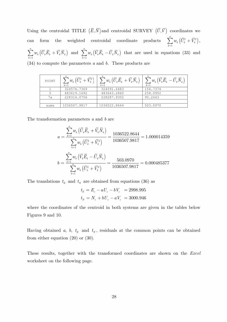
Using the centroidal TITLE ( ),E N and centroidal SURVEY ( ),U V coordinates we
can form the weighted centroidal coordinate products ( )2 2
1
n
k k kk
w U V=
+∑ ,
( )1
n
k k k k kk
w U E V N=
+∑ and ( )1
n
k k k k kk
w V E U N=
−∑ that are used in equations (33) and
(34) to compute the parameters a and b. These products are
POINT ( )2 2
1
n
k k kk
w U V=
+∑ ( )1
n
k k k k kk
w U E V N=
+∑ ( )1
n
k k k k kk
w V E U N=
−∑
1 324574.7369 324591.6483 154.7374 5 483619.1692 483643.2860 258.0952 7a 228314.0756 228287.9302 90.2643
sums 1036507.9817 1036522.8644 503.0970
The transformation parameters a and b are
( )
( )1
2 2
1
1036522.8644 1.0000143591036507.9817
n
k k k k kk
n
k k kk
w U E V Na
w U V=
=
+= = =
+
∑
∑
( )
( )1
2 2
1
503.0970 0.0004853771036507.9817
n
k k k k kk
n
k k kk
w V E U Nb
w U V=
=
−= = =
+
∑
∑
The translations and are obtained from equations (36) as Et Nt
2998.995
3000.946E c c c
N c c c
t E aU bV
t N bU aV
= − − =
= + − =
where the coordinates of the centroid in both systems are given in the tables below
Figures 9 and 10.
Having obtained a, b, and , residuals at the common points can be obtained
from either equation (20) or (30). Et Nt
These results, together with the transformed coordinates are shown on the Excel
worksheet on the following page.
28

LEA
ST S
QU
AR
ES S
OLU
TIO
N O
F PA
RA
ME
TER
S O
F 2D
LIN
EAR
CO
NFO
RM
AL
TRA
NS
FOR
MA
TIO
NC
onfo
rmal
Tra
nsfo
rmat
ion
Exe
rcis
e
2D L
inea
r Con
form
al T
rans
form
atio
n (w
ith w
eigh
ts)
E =
+a*U
+ b
*V +
t(E)
E,N
are
coo
rdin
ates
in S
yste
m 1
.
N =
-b*U
+ a
*V +
t(N
)U
,V a
re c
oord
inat
es in
Sys
tem
2.
t(E) a
nd t(
N) a
re E
ast a
nd N
orth
tran
slat
ions
.R
otat
ions
are
con
side
red
posi
tive
anti-
cloc
kwis
e.U
,V c
oord
inat
es (S
yste
m 2
) are
tran
sfor
med
(sca
led,
rota
ted
and
trans
late
d) in
to E
,N c
oord
inat
es (S
yste
m 1
).
POIN
TE
NE(
c)N
(c)
UV
U(c
)V(
c)W
eigh
tE
NW
*(U
(c)^
2+V(
c)^2
)W
*(U
(c)*
E(c)
+V(c
)*N
(c))
W*(
V(c)
*E(c
)-U(c
)*N
(c))
150
00.0
0050
00.0
0011
2.08
8-1
41.0
5720
00.0
0020
00.0
0011
2.15
0-1
40.9
9610
-0.0
050.
004
3245
74.7
369
3245
91.6
483
154.
7374
546
41.1
1653
30.3
33-2
46.7
9618
9.27
616
40.9
6623
30.1
31-2
46.8
8418
9.13
55
0.00
0-0
.019
4836
19.1
692
4836
43.2
860
258.
0952
7a50
01.0
0656
05.2
4611
3.09
446
4.18
920
00.7
7426
05.2
8311
2.92
446
4.28
71
0.05
60.
050
2283
14.0
756
2282
87.9
302
90.2
643
Cen
troid
4887
.911
651
41.0
569
Cen
troid
1887
.850
321
40.9
961
Sum
s10
3650
7.98
1710
3652
2.86
4450
3.09
70
LEA
ST
SQ
UA
RE
S S
OLU
TIO
Na
= 1.
0000
1435
9t(E
) =
2998
.995
Scal
e =
1.00
0014
476
b =
0.00
0485
377
t(N) =
30
00.9
46R
otat
ion
= 0.
0278
10de
gree
s (p
ositi
ve a
nti-c
lock
wis
e)
TRA
NS
FOR
ME
D C
OO
RD
INA
TES
E =
+a*U
+ b
*V +
t(E)
N =
-b*U
+ a
*V +
t(N
)
SUR
VEY
TITL
EPo
int
UV
EN
120
00.0
0020
00.0
0049
99.9
9550
00.0
04R
M (C
ontro
l Poi
nt)
516
40.9
6623
30.1
3146
41.1
1653
30.3
14O
P (C
ontro
l Poi
nt)
7a20
00.7
7426
05.2
8350
01.0
6256
05.2
96O
P (C
ontro
l Poi
nt)
220
01.1
5320
01.7
7150
01.1
4850
01.7
75po
st3
1980
.920
2013
.194
4980
.921
5013
.208
post
415
88.6
9322
39.7
8845
88.7
9852
39.9
95po
st6
1799
.672
2605
.082
4799
.957
5605
.192
post
7b20
00.8
9726
05.2
8650
01.1
8556
05.2
99po
st8
1980
.834
2330
.297
4980
.989
5330
.315
post
4.1
1586
.088
2238
.972
4586
.193
5239
.181
RM
Sou
th W
est c
orne
r
Res
idua
lsW
eigh
ted
Cen
troid
al C
oord
inat
e Pr
oduc
tsSY
STE
M 1
(TIT
LE)
Cen
troid
al C
oord
sSY
STE
M 2
(SU
RVE
Y)C
entro
idal
Coo
rds
29
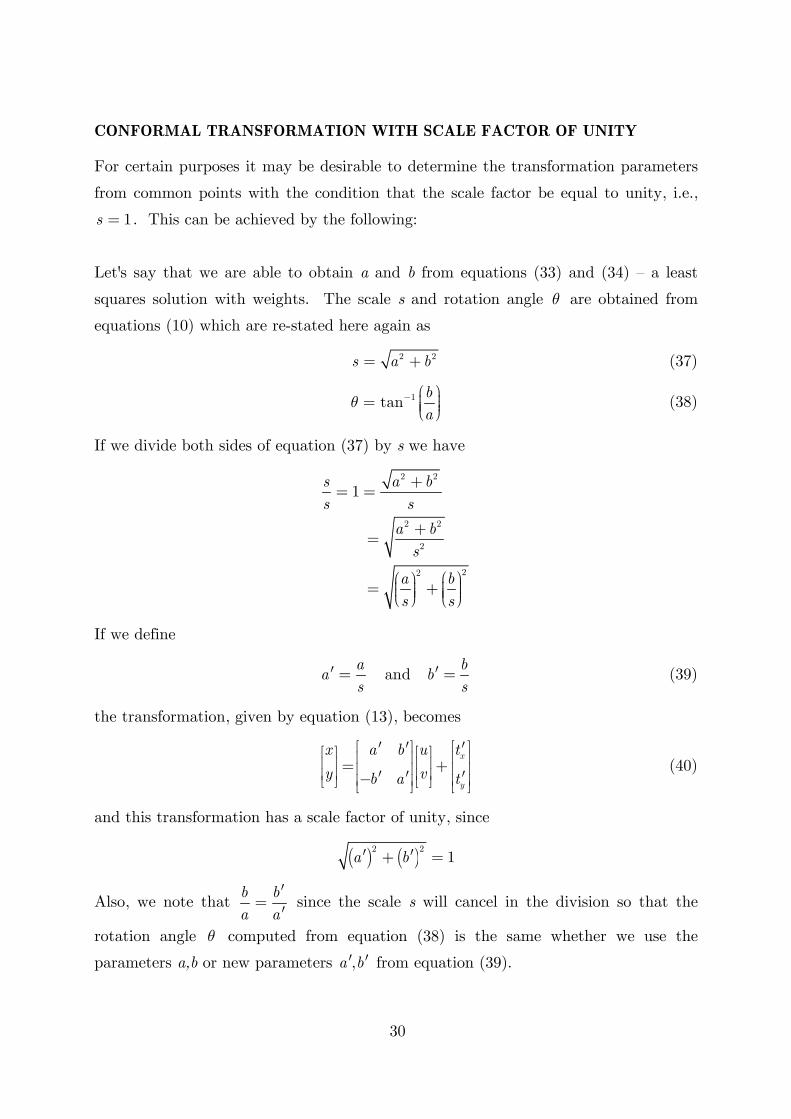
CONFORMAL TRANSFORMATION WITH SCALE FACTOR OF UNITY
For certain purposes it may be desirable to determine the transformation parameters
from common points with the condition that the scale factor be equal to unity, i.e.,
. This can be achieved by the following: 1s =
Let's say that we are able to obtain a and b from equations (33) and (34) – a least
squares solution with weights. The scale s and rotation angle θ are obtained from
equations (10) which are re-stated here again as
2s a b= + 2 (37)
1tan ba
θ − ⎛ ⎞⎟⎜= ⎟⎜ ⎟⎜⎝ ⎠ (38)
If we divide both sides of equation (37) by s we have
2 2
2 2
2
22
1s a bs s
a bs
a bs s
+= =
+=
⎛ ⎞⎛ ⎞ ⎟⎟ ⎜⎜= + ⎟⎟ ⎜⎜ ⎟ ⎟⎜⎝ ⎠ ⎝ ⎠
If we define
and aas s
′ = bb′ = (39)
the transformation, given by equation (13), becomes
x
y
x a b u ty vb a t
⎡ ⎤ ⎡′ ′ ′⎡ ⎤ ⎡ ⎤ ⎤⎢ ⎥ ⎢⎢ ⎥ ⎢ ⎥= ⎥+⎢ ⎥ ⎢⎢ ⎥ ⎢ ⎥′ ′ ′− ⎥⎢ ⎥ ⎢⎣ ⎦ ⎣ ⎦ ⎥⎣ ⎦ ⎣ ⎦
(40)
and this transformation has a scale factor of unity, since
( ) ( )2 21a b′ ′+ =
Also, we note that b ba a
′=
′ since the scale s will cancel in the division so that the
rotation angle θ computed from equation (38) is the same whether we use the
parameters a,b or new parameters from equation (39). ,a b′ ′
30

31
yt ′
c
v′
It should be noted that the "new" transformation, with scale factor of unity, given by
equation (40), has translations and these will be different from the translations
of equation (13). The translations are obtained by re-arranging
equation (40) and replacing x,y and u,v with the coordinates of the centroid and
giving
,x yt t′ ′
,x yt t and xt ′
,c cx y
,c cu v
x c
c cy
t x a b uyt b a
⎡ ⎤ ⎡ ⎤′ ′⎡ ⎤ ⎡⎢ ⎥ ⎢ ⎥ ⎤⎢ ⎥= −⎢ ⎥ ⎢ ⎥ ⎢ ⎥⎢ ⎥′ ′−⎢ ⎥ ⎢ ⎥ ⎢ ⎥′⎣ ⎦ ⎣⎣ ⎦ ⎣ ⎦ ⎦
c
c
′
′
(41)
or (42) x c c
y c c
t x a u b v
t y b u a v
′ ′= − −
′ ′= + −
After calculation of the parameters, T
x ya b t t⎡ ⎤′ ′ ′ ′= ⎢ ⎥⎣ ⎦x the residuals are calculated
using (31).
We define , , ,x yt′ ′ ′ ′a b t as the parameters of a conformal transformation with a scale
factor of unity.
Using the computed data from the example:
14476 and from equations
1.000014359, 0.000485377a b= =
giving s = (39) 1.0000
1.000014359 0.9999998821.0000144760.000485377 0.0004853701.000014476
aasbbs
′ = = =
′ = = =
The translations and are obtained from equations (42) as Et ′ Nt ′
2999.022
3000.977E c c c
N c c c
t E a U b V
t N b U a V
′ ′ ′= − − =
′ ′ ′= + − =
where the coordinates of the centroid in both systems are given in the tables below
Figures 9 and 10.
Having obtained a', b', and , residuals at the common points can be obtained
from either equation (20) or (30) by replacing a, b, and with a', b', and . Et ′ Nt ′
xt yt Et ′ Nt ′
These results, together with the transformed coordinates (where the scale factor is
unity) are shown on the Excel worksheet on the following page.

LEA
ST
SQ
UA
RE
S S
OLU
TIO
N O
F PA
RA
MET
ER
S O
F 2D
LIN
EA
R C
ON
FOR
MA
L TR
AN
SFO
RM
ATIO
NC
onfo
rmal
Tra
nsfo
rmat
ion
Exer
cise
2D L
inea
r Con
form
al T
rans
form
atio
n (w
ith w
eigh
ts)
E =
+a*U
+ b
*V +
t(E)
E,N
are
coo
rdin
ates
in S
yste
m 1
.
N =
-b*U
+ a
*V +
t(N
)U
,V a
re c
oord
inat
es in
Sys
tem
2.
t(E) a
nd t(
N) a
re E
ast a
nd N
orth
tran
slat
ions
.R
otat
ions
are
con
side
red
posi
tive
anti-
cloc
kwis
e.U
,V c
oord
inat
es (S
yste
m 2
) are
tran
sfor
med
(sca
led,
rota
ted
and
trans
late
d) in
to E
,N c
oord
inat
es (S
yste
m 1
).
POIN
TE
NE(
c)N
(c)
UV
U(c
)V(
c)W
eigh
tE
NW
*(U
(c)^
2+V(
c)^2
)W
*(U
(c)*
E(c)
+V(c
)*N
(c))
W*(
V(c)
*E(c
)-U(c
)*N
(c))
150
00.0
0050
00.0
0011
2.08
8-1
41.0
5720
00.0
0020
00.0
0011
2.15
0-1
40.9
9610
-0.0
050.
004
3245
74.7
369
3245
91.6
483
154.
7374
546
41.1
1653
30.3
33-2
46.7
9618
9.27
616
40.9
6623
30.1
31-2
46.8
8418
9.13
55
0.00
0-0
.019
4836
19.1
692
4836
43.2
860
258.
0952
7a50
01.0
0656
05.2
4611
3.09
446
4.18
920
00.7
7426
05.2
8311
2.92
446
4.28
71
0.05
60.
050
2283
14.0
756
2282
87.9
302
90.2
643
Cen
troid
4887
.911
651
41.0
569
Cen
troid
1887
.850
321
40.9
961
Sum
s10
3650
7.98
1710
3652
2.86
4450
3.09
70
LEA
ST
SQ
UA
RE
S S
OLU
TIO
Na
= 1.
0000
1435
9t(E
) =
2998
.995
Scal
e =
1.00
0014
476
b =
0.00
0485
377
t(N) =
30
00.9
46R
otat
ion
= 0.
0278
10de
gree
s (p
ositi
ve a
nti-c
lock
wis
e)
TRA
NSF
OR
ME
D C
OO
RD
INA
TES
E =
+a*U
+ b
*V +
t(E)
N =
-b*U
+ a
*V +
t(N
)
SUR
VEY
TITL
EPo
int
UV
EN
120
00.0
0020
00.0
0049
99.9
9550
00.0
04R
M (C
ontro
l Poi
nt)
516
40.9
6623
30.1
3146
41.1
1653
30.3
14O
P (C
ontro
l Poi
nt)
7a20
00.7
7426
05.2
8350
01.0
6256
05.2
96O
P (C
ontro
l Poi
nt)
220
01.1
5320
01.7
7150
01.1
4850
01.7
75po
st3
1980
.920
2013
.194
4980
.921
5013
.208
post
415
88.6
9322
39.7
8845
88.7
9852
39.9
95po
st6
1799
.672
2605
.082
4799
.957
5605
.192
post
7b20
00.8
9726
05.2
8650
01.1
8556
05.2
99po
st8
1980
.834
2330
.297
4980
.989
5330
.315
post
4.1
1586
.088
2238
.972
4586
.193
5239
.181
RM
Sou
th W
est c
orne
r
LEA
ST
SQ
UA
RE
S S
OLU
TIO
N (
SCA
LE F
AC
TOR
OF
UN
ITY
)a'
=
0.99
9999
882
t'(E)
=
2999
.022
Scal
e =
1.00
0000
000
b' =
0.
0004
8537
0t'(
N) =
30
00.9
77R
otat
ion
= 0.
0278
10de
gree
s (p
ositi
ve a
nti-c
lock
wis
e)
TRA
NSF
OR
ME
D C
OO
RD
INA
TES
E =
+a'*U
+ b
'*V +
t'(E
)N
= -b
'*U +
a'*V
+ t'
(N)
SUR
VEY
TITL
EPo
int
UV
EN
120
00.0
0020
00.0
0049
99.9
9350
00.0
06R
M (C
ontro
l Poi
nt)
516
40.9
6623
30.1
3146
41.1
1953
30.3
12O
P (C
ontro
l Poi
nt)
7a20
00.7
7426
05.2
8350
01.0
6156
05.2
89O
P (C
ontro
l Poi
nt)
220
01.1
5320
01.7
7150
01.1
4750
01.7
77po
st3
1980
.920
2013
.194
4980
.919
5013
.210
post
415
88.6
9322
39.7
8845
88.8
0252
39.9
94po
st6
1799
.672
2605
.082
4799
.959
5605
.186
post
7b20
00.8
9726
05.2
8650
01.1
8456
05.2
92po
st8
1980
.834
2330
.297
4980
.987
5330
.313
post
4.1
1586
.088
2238
.972
4586
.197
5239
.179
RM
Sou
th W
est c
orne
r
Res
idua
lsW
eigh
ted
Cen
troid
al C
oord
inat
e Pr
oduc
tsSY
STE
M 1
(TIT
LE)
Cen
troid
al C
oord
sSY
STE
M 2
(SU
RVE
Y)
Cen
troid
al C
oord
s
32

WEIGHTING SCHEMES
When solving for the transformation parameters, observation equations are
formed – there are 2n equations, where n is the number of common points or control
points – and the least squares principle leads to a set of normal equations [see
equations (24) and (25)] that involve a (diagonal) weight matrix W where the
elements of the leading diagonal etc. are known as 1 2 3, , ,w w w … weights and are
usually integers (see page 19). High weights (large integers) are associated with
"strong" points and low weights (small integers) associated with "weak" points.
This association may be best explained by reference to the example (see Figures
8 and 9) remembering that weights are only assigned to control points.
The three control points are the Reference Mark (RM found) near the S.E.
corner of Lot 1, the old peg (OP) by the post at the N.E. corner of Lot 2 and the OP
at the S.W. corner of Lot 2. Most surveyors would probably regard RM's and pegs
(if they have not been disturbed) as very strong indicators of title corners (via title-
connections in the case of RM's). Pegs might be slightly less well regarded as they
could have been disturbed, and fence posts or fence intersections, would rank below
that of pegs and RM's as important indicators of title corners. This would be a fairly
normal hierarchy that a surveyor would gain from experience. Assigning weights is
merely putting numbers into the transformation process that reflect that hierarchy.
In the exercise, the RM has been assigned a weight of 10, the OP at the S.W.
corner of Lot 2 has been assigned a weight of 5 and the other OP at the N.E. corner
of Lot 2 has been assigned a weight of 1. Perhaps here, the intention is to give less
weight to the OP by the fence post, since there is a possibility that the peg could
have been disturbed – by the fencing contractor perhaps. These are arbitrary
numbers and are reflections of the surveyor's field experience. Control points of high
weight will have smaller residuals than control points of low weight. You can adjust
the magnitude of the weights to give a particular point (or points) lower residuals
than other points.
It is interesting to note that in the Excel spreadsheet used to compute the
transformation parameters, assigning a weight of zero effectively removes that point
as a control point. This means that initially, all the occupation (RM's, OP's, posts,
etc.) can be control points in an initial transformation and then removed from the
process by assigning a weight of zero to points that have large residuals; indicating
33

34
that the occupation is not at, or near, a title corner. This adds flexibility to the re-
establishment analysis.
REFERENCES
Allan, Arthur L., 1997, Maths for Map Makers, Whittles Publishing, UK.
Bebb, G., 1981, 'The applications of transformations to cadastral surveying', Information-
Innovation-Integration: Proceedings of the 23rd Australian Survey Congress, Sydney,
March 28 – April 3, 1981, The Institution of Surveyors Australia, pp. 105-117.
Bellman, C. Deakin, R. and Rollings, N., 1992, 'Colour photomosaics from digitized aerial
photographs', Looking North: Proceedings of the 34th Australian Surveyors Congress,
Cairns, Queensland, May 23-29, 1992, The Institution of Surveyors Australia, pp. 481-495.
Bervoets, S.G., 1992, 'Shifting and rotating a figure', Survey Review, Vol. 31, No. 246,
October 1992, pp. 454-464.
Bird, D., 1984, 'Letters to the Editors: Least squares reinstatement', The Australian
Surveyor, Vol. 32, No. 1, March 1984, pp. 65-66.
Deakin, R. E., 1998, '3D coordinate transformations', Surveying and Land Information
Systems, Vol. 58, No. 4, Dec. 1998, pp. 223-34)
DSB, 1972, Dictionary of Scientific Biography, Vol. VI, C.C. Coulston Editor in Chief,
Charles Scribner's Sons, New York.
Helmert, F.R., 1880, Die mathematischen und physikalischen Theorem der höheren Geodäsie,
Vol. 1, Die mathematischen Theorem, Leipzig.
Helmert, F.R., 1884, Die mathematischen und physikalischen Theorem der höheren Geodäsie,
Vol. 2, Die physikalischen Theorem, Leipzig.
Jordan/Eggert/Kneissl, 1963, Handbuch der Vermessungskunde (Band II), Metzlersche
Verlagsbuchhandlung, Stuttgart.
Lauf, G.B., 1983, Geodesy and Map Projections, TAFE Publications, Collingwood.
Mikhail, E. M., 1976, Observations and Least Squares, IEP−A Dun-Donelley, New York.
Moffitt, F. H. and Mikhail, E. M., 1980, Photogrammetry, 3rd ed, Harper & Row, New York.
Shmutter, B and Doytsher, Y., 1991, 'A new method for matching digitized maps', Technical
Papers 1991 ACSM-ASPRS Annual Convention, Baltimore, USA, Vol. 1, Surveying, pp.
241-246.
Sprott, J. S., 1983, 'Least squares reinstatement', The Australian Surveyor, Vol. 31, No. 8,
December 1983, pp. 543-556.