coordinate systems - university of alaska fairbanks fresco/nrm340...chapter 4: coordinate systems...

Chapter 4:

Coordinate Systems

C oordinate systems are the most fundamental "link" between maps and the world they represent. They are also the critical link between GPS receivers and the physical world around us. In fact, it is not exaggerating to say that coordinates are

8 .

I the foundation of the GPS system. This chapter describes and explains the primary coordinate systems that are used in GPS receivers and on USGS topographic maps.

Coordinates define precise physical locations in remarkably simple and elegant terms. Six digits of latitude and seven digits of longitude

7iic&.it takes to specify a location to within 50 feet of precision - anywhere on earth!

GPS represents such a remarkable advance in navigation technology that it can allow land navigators to function effectively without any use of maps. Try that with a compass! Coordinates are the key to this functionality. Indeed, GPS has made it possible to use waypoint coordinates in their raw numeric form to precisely navigate complex.. routes with no map and no difficulty.

Nonetheless, maps continue to play a major role in land navigation. Maps supply an important description of the landscape within which coordinates Lie. GPS can both enhance your use of maps, and free you from the necessity of using maps. It's up to you.

As mentioned earlier, there are two basic categories of coordinate systems used in cartography and navigation. The most Oamiliar

Coordinates are the foundation of the Global Positioning System ...y ou can use them to navigate complex routes with ease.

Chapter 4: Coordinate Systems

category of coordinate system relies on angular measurements - usually degrees, minutes, and seconds - to represent actual locations on earth. The other category of coordinate system relies on rectangular measurements - Cartesian coordinates expressed in feet or meters - to represent actual locations on the earth. You will probably find both of these coordinate systems useful when you work with maps and GPS receivers.

1 Angular Coordinates Angular coordinates are the basis for the familiar latitude and longitude lines found on most maps. If you look at a side view of the earth, with the north pole at the top, lines of latitude are circles that are parallel to the equator and to one another. That's why lines of latitude are also called "parallels." Lines of longitude are half-circles that extend from the north pole to the south pole. Lines of longitude are also called "rne&liaas".

Figure 4-1: Lines Of Latitude And Longitude Wrap Around The Globe That Is The Earth - They Look Like A Grid, But They're Actually Formed By Rays

1 08

Angular Coordinates

Lines of latitude run east-west, but they are used to measure north-south distances. All points on a particular line of latitude ark the same angular and linear distance north or south of the equator (or any other specific parallel).

Lines of longitude run north-south, but they are used to measure east-west distances. All points on the same line of longitude are the same angular distance east or west of the "prime meridian" (or any other specific meridian). Since lines of longitude converge at the north and south poles, the linear distance between any two meridians is not constant. The linear distance between any two meridians is greatest at the equator and shrinks to zero at the two poles.

Angular coordinates are designed for the spherical surface of the earth. They specify points based on an angular distance from a reference point. That point is the intersection of the equator and the "prime meridian." In a moment you'll see how this reference point, or "origin," is selected.

There are a variety of different units used for angular measurements. They include degrees, mils, radians, and grads. Each divides the circumference of a circle into a number of equal arc segments. Degrees divide a circle into 360 arc segments, mils divide a circle into 6,400 arc segments, radians divide a circle into 2*pi arc segments, and gads divide a circle into 400 arc segments.

Degrees Mils

Grads Radians

Examples Of Different Angular Units - Different Ways Of Dividing Circles

1 09


Degrees are the only type of angular measurement of concern to civilian land navigators. A degree ('1360 of a circle) can be broken down further into minutes ('160 of a degree, or '/21,600 of a circle), and minutes can be divided further into seconds ('160 of a minute, or '/1.296,000 of a circle).

4.1 .I Building Angular Coordinates - From Scratch

To really understand geographic coordinates (latitude and longitude) it helps to start in two dimensions - a circle. Any point on a circle can be can be specified (relative to some other point on the circle) by the angle of the arc between the rays that pass through the two points. Figure 4-3 shows three rays that originate at the center of a circle. The angle between those rays is the angular distance between the points. An important observation is that we don't measure absolute length with an arc, only an angle. The exact sarqe angular distance will have completely different absolute lengths on circles of different diameters.

Now consider a sphere. Any point on a sphere can be specified (relative to some other point on the sphere) by two angles measured on "right circles" (see Figure 4-5). The

*

right circles are formed by the intersection of the sphefe and two planes. The planes both pass through the center of the sphere and a common point on its surface, and they are at

0" Angles are the amount of arc between two rays. Angles don't measure distance (notice the different length of thetwo 30" arcs).

Angles can be measured in either a clockwise or a counter clockwise direction. Thus the same two rays can have two different angular values (see the 60" counter clockwise arc and the

. 300" clockwise arc, or the 30" clockwise arc and the 330" counterclockwise arc).

In geographic coordinates (latitude and longitude) the rays tha t are being measured s ta r t a t the center of the earth and pass through points on the surface of the earth.

In compass directions the rays t h a t are being measured s ta r t a t a location on the surface of the earth and point in a horizontal direction.

Figure 4-3: Measuring Angles - The Foundation Of Angular Coordinate Systems

110

Angular Coordinates

right angles to each other. Notice that neither right circle needs to pass through the point being measured.

In effect, once the right circles are specified, two numbers (angles) can be used to uniquely i d e n w any point on the sphere. These angles (that we call coordinates) really specify the angle of a ray in 3-dimensional space. That ray originates from the exact center of the sphere and passes through the point we are measuring on the sphere's surface.

Something that should be noted at this point is the term "sphere" is being used loosely when it is applied to the earth. In reality, ellipsoids have been used to represent the earth's surface at sea level for well over a century. Ellipsoids are just flattened spheres. The earth is slightly flattened at the poles and bulges 'at the equator. That bulge is the result of the earth's axial spin. This discussion refers to the earth as a sphere strictly for the sake of simplicity, and nothing of importance is lost in the process. Now, back to the "spherical" model of the earth.

Angular coordinates alone do not tell you the size - the radius - of the sphere being described. In the case of the earth, the coordinates pertain to a sphere whose radius is the distance from the center of the earth to mean sea level. In other words, the "surface of the sphere" is mean sea level in the case of the earth. A third number, elevation, specifies the height of a point above, on, or below the surface of that sphere.

Elevation is relevant because it is needed to complete the full 3-dimensional specification of a point in space (or on the irregular surface of the earth). For the most part, elevation is not an essential item of information for GPS land navigation - you already know you're on the surface of the earth. In certain situations, however, elevation can be very critical when you're using GPS. See page 41 for a discussion of the role of elevation and 2D operating gode. See page 55 for a discussion of why altimeters are better than GPS receivers for giving your elevation.

One of the basic issues encountered when you work with coordinates on a sphere is how to determine a suitable point to represent the origin - the place on the surface of the sphere where the two right circles intersect. If you think about it, a sphere has no beginning and no end, nor any comers such as you find on a rectangle. Ultimately, the selection of a reference point for the origin is arbitrary. Fortunately, certain physical characteristics of the sphere we're concerned with - the earth - offer a partial answer to our need for a reference point, the "origin."

Since the earth spins around an axis (thereby giving us night and clay), we can conveniently use this spin axis as the starting point for aligning the right planes. Start by aligning one plane with this polar axis. It follows that a second right plane must be perpendicular to the spin axis. In fact, to pass through the center of the sphere the second plane must divide the earth at a distance exactly halfway between the poles. Its intersection with the sphere forms the circle we call the equator.


And South Poles -They Are The Axis Around Which The Earth Spins

e Polar Axis Is The Foundation For Positioning The Right Planes That Are The Heart Of The Geographic Coordinate System

Figure 4-4. The Earth's Spin Axis Is The Starting Point For The Angular Coordinate System

At this point the second plane (and along with it, the circle called the equator) is fixed in place, but the first plane is not. All that is specified for the first plane is that it must pass through the polar axis. It can intersect the equator anywhere. An infinite number of possibilities exist for this "polar plane." Indeed, there is more than one such plane used on various maps of the world.

Any point on earth (except the exact north or south pole) can be designated to have the first plane pass through it, and thereby fix the circle that gives us the "prime meridian." Once this is done, the intersection of the equator and the "prime meridian" establish our spherical reference point, the "0" latitude, 0" longitude" coordinate. Note that the "prime meridian" is actually one-half of a circle. Unlike parallels, meridians only "wrap" around one-half of the earth's sphere. You would need to travel along two meridians to fully circumnavigate the globe around the poles.

The meridian designated as "prime" is given an angular value of zero. All other meridians can be specified by the angle their plane forms with the prime meridian. Meridians (lines of longitude) are labeled in terms of their angle either east or west of the prime meridian (0" longitude). This limits meridians to values between 0" and 180". They must, however, be labeled as east (E) or west (W) to cover the full 360" arc of the equator (or whatever parallel the point is on).

Angular Coordinates

Meridians converge at the poles, so they appear on the surface of the earth similar to the segments of an orange. All points along the same meridian are the same number of degrees east or west of the prime meridian. The angular distance between any two meridians, measured in degrees, is the same regardless of whether the degrees are measured at the equator or at the arctic circle. The linear distance between two meridians is not constant, since meridians are not parallel. On the equator each degree between meridians is about 69 miles long. At the arctic circle (latitude 66% degrees north) each degree between meridians is 26 miles long. As meridians converge at the poles, this distance shrinks to zero.

Now let's return to the equator. (Whew - it's hot and humid all of a sudden.) We can spec@ any point on a particular meridian by the angle it forms in relation to the equator. If all such points at this angle on all meridians are connected, we have a line of latitude, or a parallel. Parallels are just circles around the earth that are parallel to the equator.

Lon 60

Origin (o..oo)

Figure 4-5: Angular Coordinates On A Sphere - It's Really Just n o (Right) Circles

Chapter 4: Coordinate Systems a

Figure 4-6: Any Two Parallels -Everywhere The Same Linear Distance Apart

The angle of a parallel can be from 0" (the equator ) to 90" (one or the other of the poles). To avoid using negative numbers we, need to indicate a direction. Thus, lines of latitude (parallels) are specified as being north (N) or south (S) of the equator. Since they range from 0" to 90" (plus N or S for hemisphere), they cover a pole to pole arc of 180".

Figure 4-7: Any Two Meridians -Ever Changing Linear Distance ,

I

Angular Coordinates 'jii

Figure 4-8: All Possible Rays Through A Parallel Fonn A Cone

Parallels are on planes that "slice" the polar axis of the earth at right angles, but the "rays" that make up each parallel actually form a cone. The point of the cone is located at the exact center of the earth, and it radiates out around the polar axis. It passes through the surface of the earth at a right angle to the surface.

Figure 4-9: All Possible Rays Through A Meridian Form One-Half Of A Plane


4.1.2 Latitude and Longitude - Putting It All Together

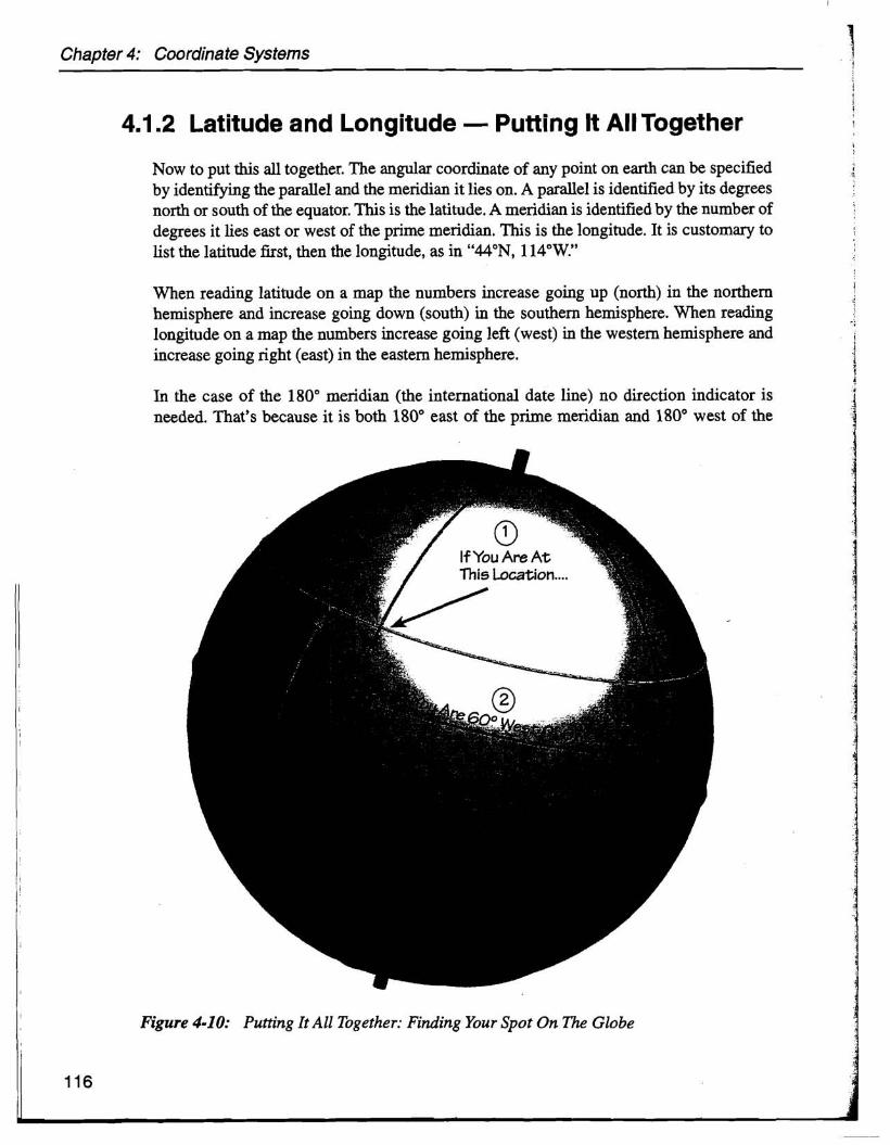
Now to put this all together. The angular coordinate of any point on earth can be specified by identifying the parallel and the meridian it lies on. A parallel is identified by its degrees north or south of the equator. This is the latitude. A meridian is identified by the number of degrees it lies east or west of the prime meridian. This is the longitude. It is customary to list the latitude first, then the longitude, as in "44"N, 114"W."

When reading latitude on a map the numbers increase going up (north) in the northern hemisphere and increase going down (south) in the southern hemisphere. When reading longitude on a map the numbers increase going left (west) in the western hemisphere and increase going right (east) in the eastern hemisphere.

In the case of the 180" meridian (the international date line) no direction indicator is needed. That's because it is both 180" east of the prime meridian and 180" west of the

Figure 4-10: Putting It All Together: Finding Your Spot On The Globe

Angular Coordinates

prime meridian. In the case of the poles (latitudes 90°N and 90"s) no longitude value is needed since all lines of longitude pass through both poles.

Angular coordinates define a specific position on a sphere of any particular radius. Since the surface of the earth is not a smooth sphere, we need a third value to fully describe a point on (or, for that matter, above or below) the earth. Elevation is that third value.

I Sometimes latitude and longitude are expressed without a letter for the hemisphere. Some

4.1.3 Elevation

i

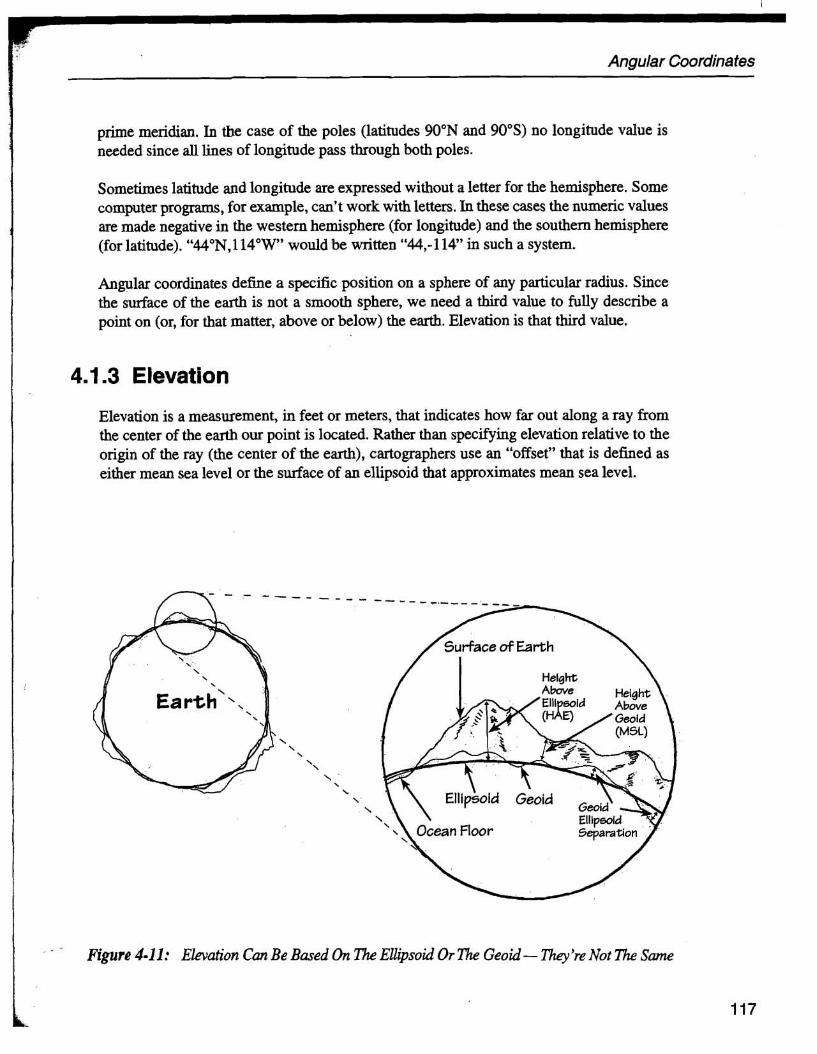
Elevation is a measurement, in feet or meters, that indicates how far out along a ray from the center of the earth our point is located. Rather than specifying elevation relative to the origin of the ray (the center of the earth), cartographers use an "offset" that is dehed as either mean sea level or the surface of an ellipsoid that approximates mean sea level.

computer programs, for example, can't work with letters. In these cases the numeric values are made negative in the western hemisphere (for longitude) and the southern hemisphere (for latitude). "44°N,1140W would be written "44,-114" in such a system.

Surface of Earth / I Helght

Figure 4-1 1: Elevation Can Be Based On The Ellipsoid Or % Geoid - They 'E Not The Same


Mean sea level (MSL) is the vertical datum used on USGS topographic maps. MSL is the earth's surface of constant gravity, and it is called the "geoid." The geoid has been described as the surface that would exist if oceans where to replace the earth's continental masses. You can think of the geoid as the gravitational equivalent of an isobar, contour line, isogonic line, etc. The geoid is obtained by local physical observations, and it is irregular over fairly small areas, such as states. See Figure 2-20 for a simulated image of how the geoid appears over the U.S.

The GPS system doesn't use the geoid as its vertical reference. Instead, it uses an ellipsoid to approximate the surface of the earth at sea level. This is a mathematical portrayal of the earth's shape. It is not the same as the surface of the geoid. The vertical difference between the ellipsoid and the geoid is up to 52 meters in the continental U.S. This means GPS elevation does not match the elevation found on most maps. However, many GPS receivers designed for personal navigation use a table to convert from ellipsoidal elevation to geoidal elevation. Doing so gets them to within about 5 meters of the elevation shown on a map.

Getting back to our coordinate system, any point's eleyation is just its vertical distance above or below either mean sea level or the surface of the ellipsoid.

4.1.4 Distance Measurement

Before leaving the topic of angulaf coordinates, we need to examine the units that are used in this system a little more closely. So far we've mostly talked about angles in terms of degrees. Each degree of latitude covers approximately 69 statute @les (or 60 nautical miles) anywhere on earth, and each degree of longitude covers approximately 69 statute miles (also 60 nautical miles) at the equator.

To get more resolution, it is possible to write decimal degrees, such as "44.3564O." One decimal place gives a resolution of 6.9 miles, two decimal places give a resolution of .69 miles, three decimal places give a resolution of 364 feet, four decimal places give a resolution of 36 feet, and so on.

Another way to obtain more resolution is to use minutes (1160th of a degree) and seconds (1160th of a minute). A minute gives resolution to 1.15 miles and a second gives resolution to 101 feet. A second carried to one decimal place gives a resolution to 10 feet!

1

Keep in mind that the foregoing values are close approximations that apply to all degrees i of latitude, but for longitude they apply only to distance measurements along the equator.

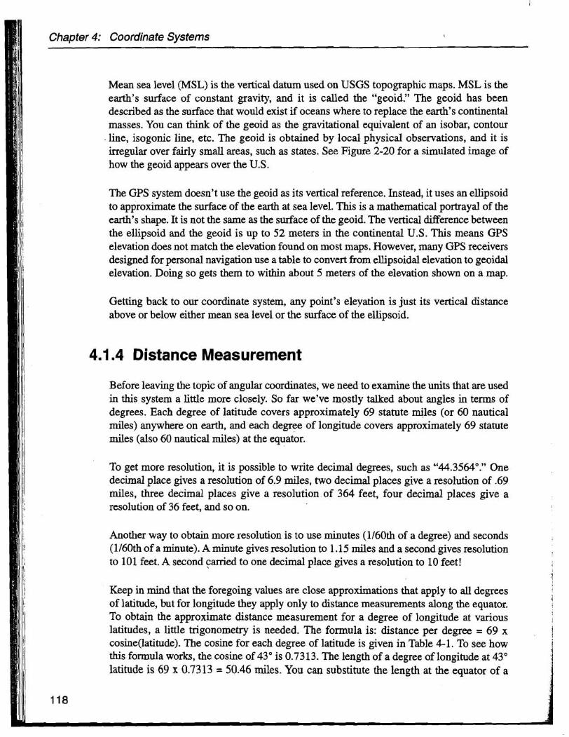
To obtain the approximate distance measurement for a degree of longitude at various latitudes, a little trigonometry is needed. The formula is: distance per degree = 69 x i

! cosine(1atitude). The cosine for each degree of latitude is given in Table 4-1. To see how this formula works, the cosine of 43" is 0.7313. The length of a degree of longitude at 43" latitude is 69 x 0.7313 = 50.46 miles. You can substitute the length at the equator of a

Angular Coordinates

Conversion Fa'actors For Angular To Linear Measurements Co.sine Latitude

O0 1 0000 Latitude Cosine Latitude Cosine . .................. ..................... ..................... lo ................. 0.9990 31° 0.0572 61° 0.4040 ..................... ..................... 2 O ................. 0.9994 32O 0.0400 62O 0.4695 ..................... 3O ................. 0.9906 33O ..................... 0.0307 63O 0.4540 ..................... 4O ................. 0.9976 34O ..................... 0.0290 64O 0.4384 .................... 5O ................. 0.9962 35O .................... 0. 0191 65O 0.4226 ..................... ..................... 6O ................. 0.9945 36O 0. 0090 66O 0.4067 ................... ................. 7 O 0.9925 37O ..................... 0. 7986 67O 0.3907 ..................... ..................... 0O ................. 0.9903 30O 0.7000 60O 0.3746 ..................... So ................. 0.9077 39O ..................... 0 . m 6S0 0.3584 ..................... lo0 ................. 0.9848 40° ..................... 0. 7660 70° 0.3420 .................... 11° ................. 0.9016 41° ..................... 0.7547 71° 0.3256 ..................... 1 2 O ................. 0.9701 42O ..................... 0.7431 7 2 O 0.3090

................. ..................... 13O 0.9744 430 ..................... 0.7313 73O 0.2924

................. ................... 14O 0.9703 44-O ..................... 0.7193 74O 02756 15O ................. 0.9659 4-5O ..................... 0.7071 75O ..................... 0.2500 16O ................. 0.9613 46O ..................... 0.6947 76O ..................... 0.2419

..................... 1 7 O ................ 0.3563 47O ..................... 0.6020 77O 0.2249

..................... 10O ................. 0.9511 40O ..................... 0.6691 70O 0. 2079

..................... IS0 ................. 0.9455 49O ..................... 0.6561 79O 0.1900 ..................... 20° ................. 0.9397 50° 0.6428 00° ..................... 0. 1736 .................... ..................... 21 O ................. 0.9336 51° 0.6293 01° 0.1564

..................... 22O ................. 0.9272 52O ..................... 0.6157 02O 0.1392 23O ................. 0.9205 53O ..................... 0.6010 03O ..................... 0.1219

..................... ..................... 24O ................. 0.9135 54O 0.5070 &I0 0.104-5 ..................... 25O ................ 0.9063 55O ..................... 0.5736 05O 0.0072 ..................... 26O ................. 0.0900 56O ..................... 0.5592 06O 0.0690

27O ................. 0.0910 57O ..................... 0.5446 07O ..................... 0.0523 20O ................. 0.0029 50O ..................... 0.5299 00O ..................... 0. 0349 29O ................. 0.07M 59O ..................... 0.5150 09O ..................... 0.0174 30° ................. 0.8660 60° ..................... 0.5000 SO0 ..................... 0.0000

-

Table 4-1: Table Of Cosines (For Converting Between Angular And Linear Measurements)

minute. second. or whatever angular unit you chose (in place of 69 miles per degree) to obtain the corresponding distance at the latitude of your choice .

4.1.5 Angular Units

When specifying angular coordinates you can choose between decimal degrees. decimal minutes or decimal seconds. but you can't mix them together . The possibilities are decimal degrees (no minutes or seconds); degrees and decimal minutes (no seconds); or degrees. minutes and decimal seconds .

To convert from decimal degrees to degrees and decimal minutes. just take the decimal component of the degree (the part to the right of the decimal place) and multiply it times 60 to get decimal minutes . To convert from decimal minutes to minutes and decimal seconds. multiply the decimal component of the minutes times 60 to get decimal seconds .


Seconds 1111) Minutes III* Degrees ..... decimal seconds 45" 37' 21.0"

u decimal minutes ..... 45" 37 21/60' = 45" 3735' u decimal degrees ............ .... ........... 45 3735/600 = 45.6225'

Degrees III* Minutes III* Seconds ..... decima I degrees 45.3725"

u decimal minutes ..... 45" 60 x .3725' = 45" 22.35'

.u decimal seconds ..................... 45" 22' 60 x .35 = 45" 22' 21.0"

Figure 4-12: Converting Between Various Units Of Angular ~easurement

To convert from decimal degrees to degrees, minutes, and decimal seconds, just calculate decimal minutes as an intermediate step.

Going the other way, to convert from decimal seconds to decimal minutes, divide the decimal seconds by 60 and add the result to the truncated minute value. To convert from decimal minutes to decimal degrees, divide the decimal minute value by 60 and add the result to the truncated degree value. To convert from decimal seconds to decimal degrees, just calculate decimal minutes as an intermediate step.

If you need to do such conversions very often, it is relatively simple to program a spreadsheet to do the conversions automatically. There are also dedicated computer programs available that will do coordinate conversions for you.

4.2 UTM Rectangular Coordinates Rectangular coordinates are a response to the weaknesses of the angular coordinate system. The Universal lkansverse Mercator system .is the "grandaddy" of the rectangular coordinate systems. It covers the entire surface of the earth, with the exceptions of the north and south polar regions. The poles are covered by a different coordinate system.

For all their elegance and precision in pinpointing any location on our spherical earth, angular coordinates can be very difficult to work with. Perhaps the most apparent acuity in working with angular coordinates is the absence of a constant distance relationship. A

UTM Rectangular Coordinates

degree of longitude ranges fiom about 69 miles long at the equator, to about 49 miles long at the 45th parallel, to about 26 miles long at the arctic circle. A degree of latitude, on the other hand, varies by a negligible amount, and is equal to about 69 miles at any parallel (and at any meridian).

Since land navigation usually involves interacting with just a small part of the world around us, a different coordinate system was devised that makes large scale maps easier to use. By specifying coordinates in a rectangular framework it is possible to directly link the coordinate numbering system to a distance measuring system. That is exactly what the Universal Transverse Mercator (UTM) coordinate system accomplishes. Each UTM coordinate grid is expressed in units of meters, with a particular point on the grid specified as the number of meters east and north of 8 reference point. There are a total of 60 separate UTM grid zones in the UTM system.

While the UTM grid system is simpler than the angular coordinate system in many ways, it is not independent of the angular system. In fact, the 60 UTM grid zones each span six degrees of longitude and 164 degrees of latitude. Each UTM grid zone extends from latitude 80"s to latitude 84"N, and is centered exactly on a line of longitude.

The regions of the earth below latitude 80"s and above latitude 84"N (the polar regions) are not included in the UTM system. Instead, they are covered by a different grid system

+ Figure 4-13: The World Is Divided Into 60 UTM Zones; There Are Also 20 Latitude Bands

Labeled C Through X


Figure 4-14: The UTM Zone Coverage Of The United States

known as UPS - the Universal Polar Stereographic system. The UPS grid system is described briefly in the next section.

The numbering system for UTM zones starts with zone number 1 at longitude 180" (the international date line) and proceeds east. UTM zone 1 extends from longitude 180°W to longitude 174"W. It is actually centered on longitude 177"W. At longitude 0" (the prime, or Greenwich meridian) we reach the eastern edge of UTM zone 30 and the western edge of UTM zone number 31. Continuing east the last UTM zone (zone number 60) begins at longitude 174% and ends at longitude 1800,' or where we started. See Figure 4-13.

In the angular coordinate system longitude values increase in both directions starting at the prime meridian. This means longitude values increase when going west in the Western Hemisphere, and when going east in the Eastern Hemisphere. The UTM grid zone numbers always increase in an easterly direction. Unfortunately, this means that UTM grid zones increase in the opposite direction as longitude in the Western Hemisphere. See Figure 4- 14.

Since a rectangular coordinate system is not capable of representing a curved surface without some distortion, the UTM coordinate system has a certain amount of distance related distortion. By using 60 separate zones this distortion is limited to less than 1 part in 2,500 parts, or less than .04 percent.

Each UTM zone is an independent Cartesian grid system that has its own origin. For each zone the origin is located at the intersection of the equator and the zone's central meridian. Thus, the origin of each zone lies on the equator and is exactly 6 degrees of longitude from the origin of adjacent UTM zones.

UTM grids are designed to be "read right then up." This means that the grid numbers always increase from left to right (west to east) and from bottom to top (south to north). Unlike the angular system, this direction of measurement does not depend on which north- south or east-west hemisphere you are working in. Anywhere on earth, the UTM rule is always "read right then up." This also means that UTM coordinates are usually given with the hoiizontal (easting) value first, then the vertical (northing) value second.

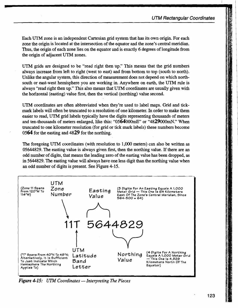
UTM coordinates are often abbreviated when they're used to label maps. Grid and tick- mark labels will often be truncated to a resolution of one kilometer. In order to make them easier to read, UTM grid labels typically have the digits representing thousands of meters and ten-thousands of meters enlarged, like this: "0564000m~ or "4829000mN." When truncated to one kilometer resolution (for grid or tick mark labels) these numbers become 0564 for the easting and 4829 for the northing.

The foregoing UTM coordinates (with resolution to 1,000 meters) can also be written as 05644829. The easting value is always given first, then the northing value. If there are an odd number of digits, that means the leading zero of the easting value has been dropped, as in 5644829. The easting value will always have one less digit than the northing value when an odd number of digits is present. See Figure 4-15.

L

UTM (Zone 11 Spans Zone (3 Dlglt6 For An Easting Equals A 1.000 From 120°W To E a s t i ng M e t e r Grld - This One I s 64 Kilometers 114'W) Number E a s t Of The Zone'e Central Merldlan, Since

5 6 4 - 5 0 0 - 64)

\ L 11T 5644829

I ii UTM (4 Digi ts For A Northing

("T" spans From 4 0 ' N To 40'N: La t i tude Northing E quale A 1 . 0 0 0 M e t e r Grld Alternatlvely. I t Is Sufficient

Band Value - Thls One Is 4 , 0 2 9 To J u s t lndlcate Which Kilometers North Of The Hemlsphere The Northlng

L e t t e r Equator) Applies To)

Figure 4-15: UTM Coordinates -Interpreting The Pieces



The I l l u s ~ o n a t left shows how the UTM coordinate systern compares to the latltudellongitude coordinate system. This illustration is not drawn to scale, since the vertical dimension wvew 20 times the distance covered by the horizontal scale. This does, however, show the essence of how the UTM coordinate system is designed.

The UTM coordinate system is overlaid on top d the gecgraphlc (latitudellongitude) coordinate system.

The two system5 coincide in each d 60 UTM zones a t the equator and a t each zone's central meridian (zone 11 is shown, with i t s central meridian d 117"W).

The boundary of each UTM zone is defined by the meridians tha t are 3" east and west d the zone's central meridiart. In this case those meridiansare 12OW and 114"W.

Om 500,000m 1,000,000m

Figure 4-16: Each UTM Zone Is Centered On A Meridian - The "Central" Meridian

The reason that the easting value requires one less digit is the "tall nanow" shape of the UTM zones. An easting value will never exceed 999,999 meters. Northing values, on the other hand, start at zero on the equator and reach about 9,300,000 meters at latitude 84" North - the northem-most reach of the UTM zones. This means that meter-level precision requires six digits for the easting and seven digits for the northing.

For a particular UTM zone seven or eight total digits specify a point to within 1,000 meters of precision, nine or ten total digits to within 100 meters of precision, eleven or twelve total digits to within 10 meters of precision, and so on. The zone designator adds two more digits, and a letter of the alphabet is used to designate the southern or northern hemisphere.

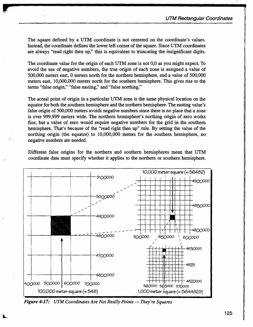
A UTM coordinate actually defmes a square area, rather than a precise point. The length of I

I the sides of the square are determined by the resolution of the coordinate pair. If the resolution is 1,000 meters, then the sides of the square are 1,000 meters long. If the

I I

resolution is 10 meters, then the square has sides that are 10 meters long. Any point that falls within a particular square will have the same coordinate (at that resolution) as any other point that falls within the same square.

I


The square defined by a UTM coordinate is not centered on the coordinate's values. Instead, the coordinate defines the lower left comer of the square. Since UTM coordinates are always "read right then up," this is equivalent to truncating the insignificant digits.

The coordinate value for the origin of each UTM zone is not 0,O as you might expect. To avoid the use of negative numbers, the true origin of each zone is assigned a value of 500,000 meters east, 0 meters north for the northern hemisphere, and a value of 500,000 meters east, 10,000,000 meters north for the southern hemisphere. This gives rise to the terms "false origin," "false easting," and "false northing."

The actual point of origin in a particular UTM zone is the same physical location on the equator for both the southern hemisphere and the northern hemisphere. The easting value's false origin of 500,000 meters avoids negative numbers since there is no place that a zone is over 999,999 meters wide. The northern hemisphere's northing origin of zero works fine, but a value of zero would require negative numbers for the grid in the southern hemisphere. That's because of the "read right then up" rule. By setting the value of the northing origin (the equator) to 10,000,000 meters for the southern hemisphere, no negative numbers are needed.

Different false origins for the northern and southern hemispheres mean that UTM coordinate data must specify whether it applies to the northern or southern hemisphere.

Figure 4-1 7: UTM Coordinates Are Not Really Points - They 're Squares

1 25


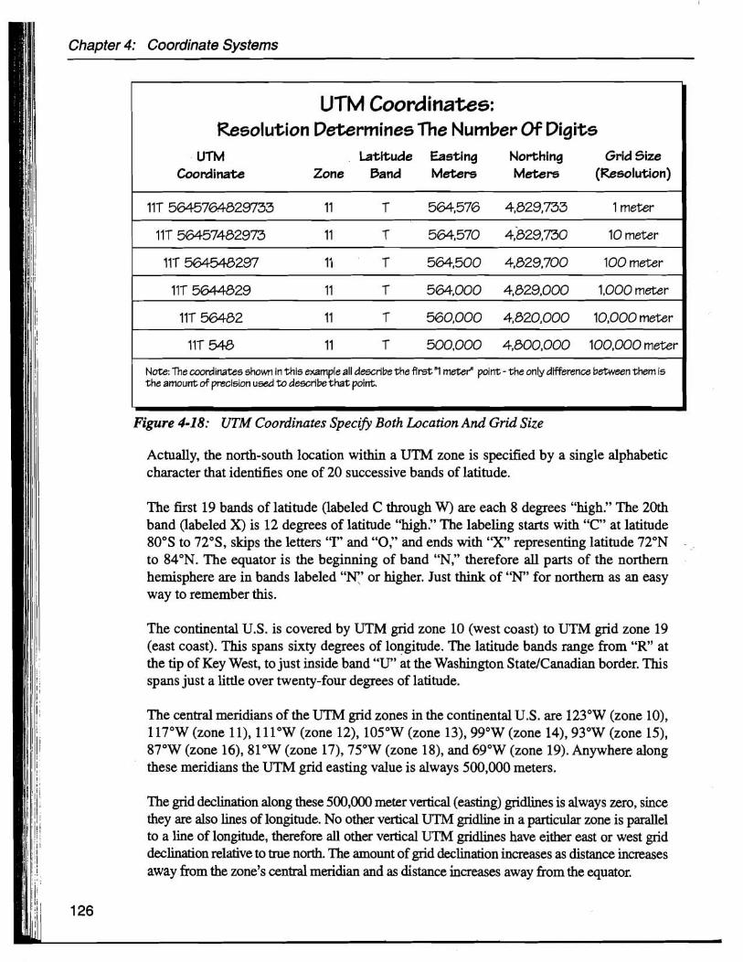
UTM Coordina=ks: Resolution Determines The Number Of Digits

UTM Latitude Easting Northing Grid Size Coordinate Zone Band Meter5 Meter5 (Kesolution)

11T 5645764629733 11 T 564,576 4,629,733 1 meter

1 IT 56457462973 11 T 564,570 4,629,730 10 meter

11T 564540297 11 T 564,500 4,629,700 100 meter

11T 5644029 11 T 564,000 4,629,000 1,000 meter

11T 56462 11 T 560,000 4,620,000 10,000 meter

11T 540 11 T 500,000 4,600,000 100,000 meter

Note: The coordinates shown in this example all descrlbe the first "1 mete?' point - the only difference between them is the amount of predsion used to describe t h a t point.

Figure 4-18: UTM Coordinates Specify Both Location And Grid Size

Actually, the north-south location within a UTM zone is specified by a single alphabetic character that identifies one of 20 successive bands of latitude.

The first 19 bands of latitude (labeled C through W) are each 8 degrees "high." The 20th band (labeled X) is 12 degrees of latitude "high." The labeling starts with "C" at latitude 80"s to 72"S, skips the letters "I" and "0," and ends with " X representing latitude 72"N - ,.

to 84"N. The equator is the beginning of band "N," therefore all parts of the northern hemisphere are in bands labeled "N,' or higher. Just think of " N for northern as an easy way to remember this.

The continental U.S. is covered by UTM grid zone 10 (west coast) to UTM grid zone 19 (east coast). This spans sixty degrees of longitude. The latitude bands range from " R at the tip of Key West, to just inside band "U" at the Washington StatelCanadian border. This spans just a little over twenty-four degrees of latitude.

The central meridians of the UTM grid zones in the continental U.S. are 123"W (zone lo),

I 117"W (zone 1 I), 11 1°W (zone 12), 105"W (zone 13), 99"W (zone 14), 93"W (zone 15),

I 87"W (zone 16), 81°W (zone 17), 75"W (zone 18), and 69"W (zone 19). Anywhere along these meridians the UTM grid easting value is always 500,000 meters.

The grid declination along these 500,000 meter vertical (easting) gridlines is always zero, since they are also lines of longitude. No other vertical UTM gridline in a particular zone is parallel to a line of longitude, therefore all other vertical UTM gridlines have either east or west grid declination relative to true north. The amount of grid declination increases as distance increases away from the zone's central meridian and as distance increases away from the equator.

Among the horizontal (northing) gridlines, only the 0 meter gridline (and its counterpart 10,000,000 meter gridline in the southern hemisphere) correspond exactly to a line of latitude - the equator. As you move north, the horizontal UTM grid lines appear to curve down and away from the lines of latitude as you move away from the zone's central meridian. This is because the lines of latitude are parallel to the equator on a spherical surface, while the UTM horizontal gridlines are parallel to the equator on a rectangular surface.

If you want to see this phenomenon for yourself, just try laying the edge of a sheet of paper flat along the 45th parallel on a globe. Now try it on the equator. The equator can be aligned along the edge of the paper, but the 45th parallel can not! It's the difference between great circles (the. equator) and little circles (other lines of latitude), concepts that are explained in the next chapter on page 146. For now you just need to see that the parallels above the equator curve up and away from the edge of the flat sheet of paper. Correspondingly, the UTM grid declination in the Northern Hemisphere is west when the easting value is less than 500,000 meters (i.e., west of the central meridian), and it is east when the easting value is greater than 500,000 meters (i.e., east of the central meridian).

4.3 Other Rectangular Coordinates There are a number of other rectangular coordinate systems besides UTM. In most situations involving GPS land navigation they do not prove to be particularly useful. The other coordinate systems listed here are included either because they are used in specialized cases for certain GPS users, or because you will encounter them on USGS topographic map products.

4.3.1 Universal Polar Stereographic (UPS)

Universal Polar Stereographic, or UPS, is a metric coordinate system that covers the extreme southern and northern latitudes. It is basically a complement to the UTM system. It relies on a different projection method to cover the extreme polar regions. It is not used anywhere in the United States.

The design of the LJPS grid is similar to UTM in that it uses a false origin. The pole (either north or south) is the projection's true origin, but the pole is given a "false" value of 2,000,000 meters North and 2,000,000 meters East. Note that the same false northing value is used at both the North Pole and the South Pole.

In the case of the North Pole, northing values are centered along the 0°/180" meridians (the prime meridian and the international date line) with values increasing as you move north along the prime meridian, then continuing to increase as you move south along the international date line. The easting values increase as you move north along the 90" West meridian, then they continue to increase as you move south along the 90" East meridian.


West Mer

East Merldlan

O" Meridian

Figure 4-19: Universal Polar Stereographic (UPS) Grid At The North Pole - It Only Applies Within The Circle Fonned By The 84" North Parallel

Figure 4-20: Universal Polar Stereographic (UPS) Grid At The South Pole - It Only Applies Within The Circle Fonned By The 80" South Parallel

lian

Other Rectangular Coo

Think of it as looking down from directly above the north pole, with the prime meridian at the bottom and the 90°W meridian on the left. See Figure 4-19.

The South Pole grid is laid out in the same way as the North Pole, except the northing value increases as you go south along the 180" longitude line, reaches 2,000,000 meters at the South Pole, then keeps increasing as you move north along the prime meridian. Think of it as looking down from directly above the south pole, with the prime meridian at the top and the 90°W meridian on the left. See Figure 4-20.

).3.2 Military Grid Reference System (MGRS)

The Military Grid Reference System, or MGRS, was developed by the U.S. Army to simplify the use of rectangular grid coordinate systems. It is a relative of the UTM and UPS grid systems.

The MGRS grid uses the same grid zone identifiers (1 through 60) and band identifiers (C through X) as the UTM system (see Figure 4-13). It then adds two letters to designate 100,000 by 100,000 meter (100 by 100 kilometer) squares. Following those two letters the MGRS system reverts to the standard UTM eating and northing values.

If two digits follow the letters, they spec@ the lower left corner of a 10,000 by 10,000 meter square. If four digits follow the letters, they specify the lower left corner of a 1,000

Figure 4-21: Military Grid Reference System 100,000 Meter Square Designations (And A Handy MGRSIUTM Converter)

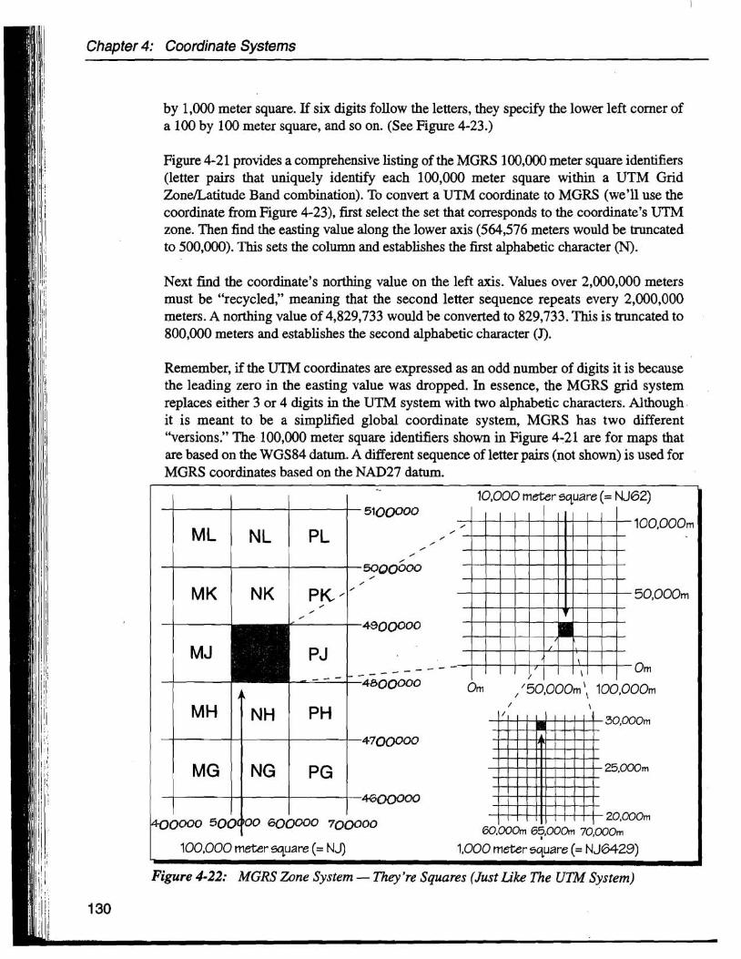
by 1,000 meter square. If six digits follow the letters, they specify the lower left comer of a 100 by 100 meter square, and so on. (See Figure 4-23.)

Figure 4-21 provides a comprehensive listing of the MGRS 100,000 meter square identifiers (letter pairs that uniquely identify each 100,000 meter square within a UTM Grid ZoneLatitude Band combination). To convert a UTM coordinate to MGRS (we'll use the coordinate from Figure 4-23), first select the set that corresponds to the coordinate's UTM zone. Then find the easting value along the lower axis (564,576 meters would be truncated to 500,000). This sets the column and establishes the first alphabetic character (N).

Next find the coordinate's northing value on the left axis. Values over 2,000,000 meters must be "recycled," meaning that the second letter sequence repeats every 2,000,000 meters. A northing value of 4,829,733 would be converted to 829,733. This is truncated to 800,000 meters and establishes the second alphabetic character (J).

Remember, if the UTM coordinates are expressed as an odd number of digits it is because the leading zero in the easting value was dropped. In essence, the MGRS grid system replaces either 3 or 4 digits in the UTM system with two alphabetic characters. Although it is meant to be a simplified global coordinate system, MGRS has two different "versions." The 100,000 meter square identifiers shown in Figure 4-21 are for maps that are based on the WGS84 datum. A different sequence of letter pairs (not shown) is used for MGRS coordinates based on the NAD27 datum.

Figure 4-22: MGRS Zone System - They're Squares (Just Like The UTM System)

Other Rectangular Coordinates

MGW Coordinates: Just A Modified Version Of UTM!

UTM MGW Grid Size Coordinate Coordinate (Resolution)

11T 5645764829733 1 IT N J64-57629733 1 meter

11T 56457462973 11T NJ64572973 10 meter

11T 564540297 11T NJW5297 100 meter

11T 564029 11T NJ6429 1,000 meter

11T 56402 1lT NJ62 10,000 meter

11T 548 11T NJ 100,000 meter

Note: The coordinates shown In this example all descrlbe the f irst "1 meter" polnt - the only difference between them is the amount of precision used to describe tha t point. See Flgure 3-18 for details of the UTM coordinate used here.

Figure 4-23: MGRS Coordinates - They're Just A Modified Fonn Of UTM!

The good news about MGRS is that it is not used on USGS 7.5-minute and 15-minute quadrangle series maps, so you probably won't need to worry about it. That's because the entire land area of the United States is covered by USGS 7.5-minute maps, and they use UTM. MGRS is a more valuable feature in a GPS receiver if you intend to use Defense Mapping Agency maps either in the U.S. or overseas.

, 4.3.3 Township and Range System (USPLSS)

I Township and Range grids are printed on all USGS topographic maps that cover areas that have been surveyed by the U.S. Public Land Survey System (USPLSS). This grid system has its origin in the Land Ordnance of 1785.

This system is built on a network of base lines and principal meridians that are lines of latitude and longitude. The intersection of the base line and the principal meridian is known as the "Initial Point." Most states have only one Initial Point, but a few states have several Initial Points. Some states, such as Oregon and Washington, share a single initial point. Figure 4-25 is a U.S. map of base lines and principal meridians.

The USPLSS grid system is built outward from the Initial Point in six mile increments. Township lines intersect the principal meridian every six miles north and south of the Initial Point, and Range lines intersect the base line every six miles east and west of the Initial Point. Each six mile by six mile square is known as a "Township." Townships are divided into 36 one mile by one mile squares known as "Sections."


Figure 4-24: USPLSS - How It Works

Townships Are 6 Mlle x 6 Mile Squares Sections Are 1 Mile x 1 Mile 5quares

Because of the distortion caused by the earth's curvature every fourth Range and Township line (in other words, every 24 miles) is "corrected" to realign it with a "standard" parallel or a "guide" meridian. This prevents the grid distortion from amplifying (relative to latitude and longitude graticules) as Townships and Ranges extend out from the Initial Point.

The result of this realignment is that townships are not always perfect six mile by:six mile squares. That's why the USPLSS grid printed on the face of many USGS topographic maps doesn't always form tidy perpendicular intersections. It is also why the USPLSS grid can't be easily converted to either the latitudeflongitude coordinate system or the UTM coordinate system.

0

1 mlle

2 mile

3 mile

4 mile

5 mile

6 mile

6 mile 5 mile 4 mlle 3 mlle 2 mile 1 mlle

The USPLSS grid system is mainly of interest to surveyors and lawyers because it is used for the legal description of public and private land ownership. However, you may be able to use the USPLSS in a pinch to find your location on a top0 map. It works by knowing that western lands were given away (to states, land grant universities, railroads, etc.) in one section increments. As a result, long straight fence lines in the backcountry usually indicate a section border. All you need to do is find the section on your top0 map. Be careful if you try this, it takes skill to match map features with the world around you.

I \ \

NE 114

160 Acres

Sections Are Further Divided Into Principal Meridian Successively Smaller Quarkrs

-

# - #

# #

#

6 5 4 3 2 1

12

13

24

25

36

1 7

1 8

19

9

16

21

8

17

20

26

,35

10

15

22

11

14

23

29 27 \ I

3z1 33 34 . . . . .

30

31

Other Rectangular Coordinates

Figure 4-25: USPLSS (Towns And Sections) Coverage Of The United States

4.3.4 State Plane Coordinate System (SPCS)

The State Plane Coordinate System (SPCS) was created in the 1930's. It represented a , substantial improvement over the older USPLSS. The continental United States was

divided into 125 zones, with each zone representing all or part of a state. In the case of states with multiple zones, the individual zones follow county borders.

State plane coordinates are similar to UTM coordinates in several respects. SPC's have false origins that always yield positive numbers for coordinates, and state plane coordinates are always read in the same "read right then up" manner as UTM. That's right, SPC's represent eastings and northings! The notation used for state plane coordinates is the easting first, then the northing, then the state, and finally the zone. It looks like this: "38 1170 feet East, 7 11391 feet North, Idaho, West Zone." In case you're wondering, that's the location of Idaho's State Capitol dome (NAD27).

That example also illustrates one of the key differences between SPC and UTM. State plane coordinates are.expressed in feet. In fact, the large scale USGS topographic maps have 10,000 foot State Plane Coordinate tick marks on the neatlines.


I

Figure 4-26: State Plane Coordinate System - Zone Coverage Of The United States

Another less obvious difference is that State Plane Coordinates are not based on a single standardized projection method. Some states (primarily those that are taller than they are wide) use a Transverse Mercator projection. Most states (all that are wider than they are tall, and some that are taller than they are wide) use the Lambert Conformal projection.

Although State Plane Coordinate tick marks are shown on the neatlines of all large scale USGS topographic maps, they are of no practical use to the backcountry land navigator. Fortunately, they don't clutter up the face of topographic maps, just the borders.

4.4 NAVSTAR's Coordinate System The NAVSTAR global positioning system uses a special coordinate system that is called "Earth Centered Earth Fixed, xyz" (ECEF). It is a three-dimensional Cartesian coordinate system that relies on the familiar right-angled x, y, and z axis system. The origin (0,0,0) is located at the center of the earth's mass. The z-axis goes through the n o d pole. The x-axis goes through the intersection of the prime meridian and the equator. The y-axis goes through the intersection of the 90" east meridian and the equator.

This system makes it easy for computers to specify points on the surface of the earth (as well as points in space above the surface of the earth) by their x,y,z coordinates. Relatively simple trigonometry can then be used to obtain distances and directions. Unlike the two-

- / '

NAVSTA R-3 Coordinate System .;

Although ECEF coordinates are very convenient in the NAVSTAR system, they are not well suited for direct human use. That's because they don't tie-in to mean sea level the way both angular coordinates and rectangular coordinates do. As such, ECEF coordinates are basically limited to use within a computer environment - such as the NAVSTAR satellites and GPS receivers.

The readouts you obtain from the screen of your GPS receiver are converted (by the receiver) from its internal ECEF format into either latitude~longitude coordinates, UTM coordinates, or whatever other coordinate system you've chosen for your display. Also, regardless of the datum being used for the display, your receiver always stores coordinates in the WGS84 (World Geodetic System 1984) datum. This is the native NAVSTAR datum. Any time you select a different datum, the displayed coordinates are being converted from WGS84.

Greenwich

Figure 4-27: NAVSTAR's Earth Centered, Earth Fixed XYZ Coordinate System

coordinate systems - university of alaska fairbanks fresco/nrm340...chapter 4: coordinate systems...

Documents