coordinate systems in geodesy - unb orbital system does not rotate with the earth~ but revolves with...
TRANSCRIPT

COORDINATE SYSTEMSIN GEODESY
E. J. KRAKIWSKYD. E. WELLS
May 1971
TECHNICAL REPORT NO. 217
LECTURE NOTESNO. 16

COORDINATE SYSTElVIS IN GEODESY
E.J. Krakiwsky D.E. \Vells
Department of Geodesy and Geomatics Engineering University of New Brunswick
P.O. Box 4400 Fredericton, N .B.
Canada E3B 5A3
May 1971 Latest Reprinting January 1998

PREFACE
In order to make our extensive series of lecture notes more readily available, we have scanned the old master copies and produced electronic versions in Portable Document Format. The quality of the images varies depending on the quality of the originals. The images have not been converted to searchable text.

TABLE OF CONTENTS
LIST OF ILLUSTRATIONS
LIST OF TABLES
l. INTRODUCTION
1.1 Poles~ Planes and -~es 1.2 Universal and Sidereal Time 1.3 Coordinate Systems in Geodesy
2. TERRESTRIAL COORDINATE SYSTEMS
2.1 Terrestrial Geocentric Systems •
2.1.1 Polar Motion and Irregular Rotation of the Earth • . • • . . • • • •
. . .
. . .
. . .
. . 2.1.2 2.1. 3
Average and Instantaneous Terrestrial Systems • Geodetic Systems • • • • • • • • • • . 1
2.2 Relationship between Cartesian and Curvilinear Coordinates • • • • • • • . • •
2.2.1 Cartesian and Curvilinear Coordinates of a
page
iv
vi
l
4 6 7
9
9
10 12 17
19
Point on the Reference Ellipsoid • • • • • 19 2.2.2 The Position Vector in Terms of the Geodetic
Latitude • • • • • • • • • • • • • • • • • • • 22 2.2.3 Th~ Position Vector in Terms of the Geocentric
and Reduced Latitudes . . • • • • • • • • • • • 27 2.2.4 Relationships between Geodetic, Geocentric and
Reduced Latitudes • . • • • • • • • • • • 28 2.2.5 The Position Vector of a Point Above the
2.2.6 Reference Ellipsoid . • • . • • • • • • . Transformation from Average Terrestrial Cartesian to Geodetic Coordinates •
2.3 Geodetic Datums
2.3.1 2.3.2 =2. 3. 3 2.3.4
Datum Position Parameters . Establishment of a Dat'lllli • . The North· American "Datum .• : . • · • • • Datum Transformations • • • •
2.4 Terrestrial Topocentric Systems
2.4.1 Local Astronomic System 2.4.2 Local Geodetic System •
2.5 Summary of Terrestrial Systems
ii
. . .
. . .• 28
31
33
36 4o 42 45
48
50 54
57

3. CELESTIAL COORDINATE SYSTEMS • •
3.1 The Ecliptic System ••. • ••••• 3.2 The Right Ascension System 3.3 The Hour Angle System ••• 3.4 The Horizon System ••••••••• 3.5 Variations of the Right Ascension System
3.5.1 Precession and Nutation 3.5.2 Mean Celestial Systems • 3.5.3 The True Celestial System 3.5.4 The Apparent Place System 3.5.5 The Observed Place System
. . . .
. . ·~
3.6 Transformation between Apparent Celestial and
page
61
63 65 67 71 73
74 76 81 83 84
Average Terrestrial Coordinate Systems • • • • • • 85 3.7 Summary of Celestial Systems • • • • • • • 87
4. THE ORBITAL COORDINATE SYSTEM 92
• 4.1 The Orbital Ellipse and Orbital. Anomalies • • • • • 92 4.2 The Orbital Coordinate System •. • • • • • · 96 4.3 Transformation from Orbital to Average Terrestrial
System. . . • • • -. • • . . • • . . • . • • . 98 4.4 Variations in the Orbital Elements 99 4.5 The Satellite ·subpoint • • • • • • • .•.• 99 4.6 Topocentric Coordinates of Satellite • • 101
• 5. SUMMARY OF COORDINATE SYSTEMS
5.1 5.2 5.3
5.4
Terrestrial Systems • • • • • • • • • Ce1estial Systems • • • • Duality Paradox in the Apparent and Observed Celestial Systems • • • • • • • • • • • • • • • The Connections between Terrestrial, Celestial and Orbital Systems • • • • • • • • • . • • • • • • • • •
REFERENCES .
r
104
104 106
1"07
108
109
APPErlDIX A: Swmnary of Reflection and Rotation ll.atrices 111
iii

Figure tio.
l-1
l-2
2-l
2-2
2-3
2-4
2-5
2-6
2-7
2-8
2-9
2-10
2-12
2-13
3-1
3-2
3-3
3-4
LIST OF ILLUSTRATIONS
Title
Terrestrial, Celestial, and OrbitaL Coordinate Systems
Types of Coordinate Systems
Polar Motion
Position of Point Moving Uniformly Along Equator ~linus Position on Actual Equator
Terrestrial and Geodetic Coordinate Systems
Transformations from Instantaneous to Average Terrestrial System
Reference Ellipsoid
Various Latitudes
Tangent Line to the Meridian Ellipse
Point Above Reference Ellipsoid
Meridian Section of the Earth
Orientation of Ellipsoid to Geoid
.& I • a
Geodetic and Local Geodetic Coordinate Systems
Equations Relating Terrestrial Systems
Ecliptic System
Right Ascension System
Hour Angle System
Time, Longitude, and Right Ascension
iv
Page
2
3
11
13
14
16
20
23
24
29
3liA
37A
51
59
64
66
68
70

·Figure No.
3-5
3-6
3-7
3-8
3-9
3-10
3-ll
4-l
4-2
4-3
4-4
5-l
Title
Horizon Sys.tem
Variations of the Celestial Right Ascension System
..
Motion of Celestial Pole
The Effect of Precession and Nutation
Mean Celestial Coordinate Systems
True.and Mean Celestial Coordinate Systems
Celestial Coordinate Systems
Orbit Ellipse
Keplerian Orbital Elements
Satellite Subpoint
Topocentric Coordinates of Satellite
Coordinate Systems
v
.:. Page
72
75
77
78
80
82
91
93
97
100
102
105

Table No.
2-1
2-2
2-3
2-4
2-5
3-1
3-2
LIST OF TABLES
Title
Parameters Defining the 1927 North American Datum
Translation Components
Example of Datum Transformations
Reference Poles~ Planes and Axes Defining Terrestrial Coordinate Systems
Transformations Among Terrestrial Coordinate Systems
Reference Poles, Planes and Axes Defining Celestial Coordinate Systems
Transformations Among Celestial Coordinate Systems
vi
Page
44
44
49
58
60
89
90


l. INTRODUCTION
These notes discuss the precise definitions of, and transformations
between, the coordinate systems to which coordinates of stations on or
above the surface of the earth are referred. To define a coordinate
system we must specify:
a) the location of the origin,
b) the orientation of the three axes,
c) the parameters {Cartesian, curvilinear) which define the
position of a point referred to the coordinate system.
The earth has two different periodic motions .in space. It rotates
about its axis, and it revolves about. the sun (see Figure 1-1). There
is also one natural satellite (the moon) and many artificial satellites
which have a third periodic motion in space: orbital motion about the
earth. These periodic motions are fundamental to the definition of
systems of coordinates and systems of time.
Terrestrial coordinate systems are earth fixed and rotate with the
earth. They are used to define the coordinates of points on the surface
of the earth. There are two kinds of terrestrial systems called
geocentric systems and topocentric systems (see Figure 1-2).
Celestial coordinate systems do not revolve but ~ rotate with the

SUN
*STAR
""'·
-- --------
EARTH'S OAIIT
EARTH•s ROTATtON
OBSERVER ON EARTH
ORBIT
/
TIER RESTRtAb , CELI!STt'Al Att:n ""'1JTAL COOROIN·ATE SYSTEMS. •. Fi.gur7 1-l~~t
1\)

3
Figure l-2. Types of Coordinate Systems.
Terrestrial
I
I l
Geocentric ~ ' Topocentric
~
I
i Celestial
I
I
' I I l
Ecliptic f-+ Right Ascension Hour Angle Horizon I
L...- J Orbital
l~....---___.

earth. They are used to define the coordinates of celestial bodies
such as stars~ There are four different celestial systems~ called the
ecliptic, right ascension~ hour angle~ and horizon systems.
The orbital system does not rotate with the earth~ but revolves
with it. It is used to define the coordinates of satellites orbiting
around the earth.
l.l POLES , PLANES AND AXES .
The orientation of axes of coordinate systems can be described in
terms of primary and secondary poles~ primary and secondary planes, and
primary~ secondary and tertiary axes.
The primary pole is the axis of symmetry of the coordinate system,
for example the rotation axis of the earth. The primary plane is the
plane perpendicular to the primary pole, for example the earth's
equatorial plane. The secondary plane is perpendicular to the
primary plane and contains the primary pole. It sometimes must be
chosen arbitrarily,.for example the Greenwich meridian plane, and
sometimes arises naturally, for example the equinoctial plane. The
secondary pole is the intersection of the primary and secondary planes.
The primary axis is the secondary pole. The tertiary axis is the primary
pole. The secondary axis is perpendicular to the other two axes,
chosen in the direction which makes the coordinate system either right
handed or left-handed as specified.
We will use either the primary plane or the primary pole, and the
primary axis to'specify the orientation of each of the coordinate
systems named above.

5
For terrestrial geocentric systems:
a) the origin is near the centre of the earth,
b) the primary pole is aligned to the earth's axis of
rotation, and the primary plane perpendicular to this pole is called
the equatorial plane,
c) the primary axis is the intersection between the
equatorial plane and the plane containing the Greenwich meridian,
d) the systems are right-handed.
For terrestrial topocentric systems:
a) the origin is at a point near the surface of the earth,
b) the primary plane is the plane tangential to the surface
of the earth at that point,
c) the primary axis is the north point (the intersection
between the tangential plane and the plane containing the earth's north
rotational pole),
d) the systems are left-handed.
For the celestial ecliptic system:
a) the origin is near the centre of the sun,
b) the primary plane is the plane of the earth's orbit,
called the ecliptic plane,
c) the primary axis is the intersection between the ecliptic
plane and the equatorial plane, and is called the vernal equinox,
d) the system is right-handed.
For the celestial right ascension system:
a) the origin is near the centre of the sun,
b) the primary plane is the equatorial plane,
c) the primary axis is the vernal equinox,

6
d) the system is right-handed.
For the celestial hour angle system:
a) the origin is near the centre of the sun,
b) the primary plane is the equatorial plane,
c) the secondary plane is the celestial meridian
containing the observer and the earth's rotation axis),
d) the system is left .. -handed.
For the celestial horizon system:
a) the origin is near the centre of the sun,
(the plane
b) the primary plane is paralle1 to the tangential plane at
the observer (the horizon plane),
c) the primary axis is parallel to the observer's north point,
d) the system is left-handed.
For the orbital system:
a) the origin is the centre of gravity of the earth,
b) the primary plane is the plane of the satellite orbit
around the earth,
c) the primary axis is in the orbital plane and is oriented
towards the point of perigee (the point at which the satellite most
closely approaches the earth) and is called the line of apsides,
d) the system is right-handed.
1.2 UNIVERSAL AND SIDEREAL TIME
Also intimately involved with the earth's periodic rotation and
revolution are two systems of time called universal (solar)· time (UT)
and sidereal time (ST). A time system is defined by specifying an

7
interval ~,d an ~= The solar day is the interval between successive
passages of the sU."l over the sa-ne terrestrial meridia."l. The sidereal
day is the interval between two successive passages of the vernal
equinox over the same terrestrial meridian. The sidereal epoch is the
angle between the vernal equinox and some terrestrial meridian: if
this is the Greenwich meridian then the epoch is Greenwich Sidereal
Time (GST). The solar epoch is rigorously related to the sidereal
epoch by a mathematical formula. Sidereal time is the parameter
relating terrestrial and celestial systems.
1.3 COORDINATE SYST&~S IN GEODESY
Geodesy is the study of the size and shape of the earth and the
determination of coordinates of points on or above the earth's surface.
Coordinates of one station are determined with respect to
coordinates of other stations by making one or more of the following
four categories of measurements: directions, distances, distance
differences, and heights. Horizontal and vertical angular measurements
between two stations on the earth (as are measured by theodolite for
example) are terrestrial directions. Angular measurements between a
station on the earth and a satellite position (as are measured by
photographing the satellite in the star background for example) are
satellite directions. Angular measurements between a station on the
earth and a star (as are measured by direct theodolite paintings on the
star for example) are astronomic directions. Distances between two
stations on the earth (as are measured by electromagnetic distance

8
measuring instruments for example) are terrestrial distances. Distances
between a station on the earth and a satellite position (as are measured
by laser ranging for example) are satellite distances~ Measurements
of the difference in distance between one station on the earth and two
other stations (as are measured by hyperbolic positioning systems for
example) are terrestrial distance differences. Measurements of the
difference in distance between one station on the earth and two satellite
positions (as are measured by integrated Doppler shift systems for
example) are satellite distance differences. All these measurements
determine the geometrical relationship between stations, and are the
subject of geometric geodesy [e.g. Bamford 1962].
Spirit level height differences and enroute gravity values are
measurements related to potential differences in the earth's gravity
field, and are the subject of physical geodesy [e.g. Heiskanen and
Moritz 1967].
The functional relationship between these measurements and the
coordinates of the stations to and from which they are made is
incorporated into a mathematical model. A unique solution for the
unknown coordinates can be obtained by applying the least squares
estimation process [Wells and Krakiwsky 1971) to the measurements
and mathematical model.
Details on coordinate systems as employed for terrestrial and
satellite geodesy can be found in Veis [1960] and Kaula [1966], and
for geodetic astronomy in Mueller [1969].

9
2. TERRESTRIAL COORDINATE SYSTEMS
In this chapter we will discuss terrestrial geocentric and
terrestrial topocentric coordinate systems.
We first discuss terrestrial geocentric systems using only
Cartesian coordinates, and considering in detail what is meant by "the
earth's axis of rotation" and "the Greenwich meridian". Then the
relationship between Cartesian and curvilinear coordinates is described.
Geodetic datums are discussed. Finally terrestrial topocentric systems
are considered, with .attention paid to what is meant by "the surface
of the earth".
2.1 TERRESTRIAL GEOCENTRIC SYSTEMS
In the introduction it was stated that for terrestrial geocentric
systems:
a) the origin is near the centre of the earth,
b) the primary pole is aligned to the earth's axis of
rotation,
c) the primary axis is the intersection between the primary
plane and the plane containing the Greenwich meridian,
d) the systems are right-handed.

10
The last specification is unambiguous. As we shall see the other
three are not. We will first discuss problems in defining the earth's
axis of rotation and the Greenwich meridian. The~ we will discuss
translations of the origin from the centre of the earth.
2.1.1 Polar Motion and Irreg~lar Rotation of the Earth
We think of the earth as rotating about a fixed axis at a uniform
rate. In fact, the axis is not fixed and the rate is not uniform.
Over 70 years ago, it was discovered that the direction of the
earth's rotation axis moves with respect to the earth's surface. This
polar motion is principally due to the fact that the earth's axes of
rotation and maximum inertia do not coincide. The resultant motion is
irregular but more or less circular and counterclockwise (when viewed
from North), with an amplitude of about 5 meters and a main period of
430 days (called the Chandler period}.
Two international organizations, the International Polar Motion
Service (IPMS) and the Bureau International de l'Heure (BIH) routinely
measure this motion through astronomic observations; the IPMS from five
stations at the same latitude, and the BIH from about ~0 stations
scattered worldwide. The results are published as the coordinates of
the true rotation axis with respect to a reference point called the
Conventional International Origin (CIO) which is the average position
of the rotation axis during the years 1900-1905( IUGG (1967) Bull Geed
86, 379 (1967) Resolution 19). Figure 2-1 shows the polar motion during 1969
as determined by IPMS and BIH.
Over 30 years ago irregularities in the rotation of the earth were

/ I
I
JAN. i969 -5
DEC.I969
Y--~-----r--------~~--~,o--------------~5~--~----~c~~~r--, 15 METERS
fTOWAROS 90° ) { 'WEST LONGITUDE \
\ / ', / >---/ IPMS
Figure 2-l. . POLAR MOTION
5
X
( TO.....a6 Gftftft'WI'Qt)

12-
discovered (other than polar motion). There are three types of
i~regularities: seasonal variations probably due to meteorological
changes or earth tides; secular decrease due to tidal friction; and
irregular fluctuations [Mueller 1969]. The seasonal variation is the
only one of these presently being taken into account, and it is more or
less reproducible from year to year, and produces a displacement along
the equator of up to 15 meters with respect to a point rotating uniformly
throughout the year (see Figure 2-2).
Because of this seasonal variation, the Greenwich m"eridian (the
plane containing the earth's rotation axis and the center of the transit
instrument at Greenwich Observatory) does not rotate uniformly.. A
ficticious zero meridian which does rotate uniformly (so far as the
effects of polar motion and seasonal variations are concerned) is
called the Mean Observatory o~ Greenwich mean astronomic meridian.
Its location is defined by the BIH.
2.1.2 Average and Instantaneous Terrestrial Systems
The average terrestrial (A. 'I'.) system is the ideal world geodetic
coordinate system (see Figure 2-3):
a) Its origin is at the centre of gravity of the earth.
b) Its primary pole is directed towards the CIO (the
average north pole of 1900-1905), and its primary plane is the plane
perpendicular to the primary pole and containing the earth's center of
gravity (the average equatorial plane).
c) Its secondary plane is the plane containing the primary

l3
+10 .
0
METERS
-10
JAN.1967 APR. JULY OCT. JAN. 1968
POSITION OF POINT MOVING UNIFORMLY ALONG Figure 2-2 •. , EQUATOR MINUS POSITION OF POtNT ON ACTUAL
EQUATOR.

X
ROTATION AXIS
OF EARTH
AVERAGE
GREENWICH
MEAN
MERIDIAN
CENTRE OF
GRAVITY
Figure ..:_-~ ..
TERRESTRIAL AND GEODETIC COORDINATE SYSTEMS

15
pole and the Mean Observatory. The intersection of these two planes is
the secondary pole, or primary axis.
d) It is a right-handed system.
We can then define the position vector Ri of a terrain point i in
terms of its Cartesian coordinates x, y, z as
X
y 2-1
z A.T.
The instantaneous terrestrial {I.T.) system is specified as follows:
a) Its origin is at the centre of gravity of the earth.
b) Its primary pole is directed towards the true (instan-
taneous)rotation axis of the earth.
c) Its primary axis is the intersection of the primary plane
and the plane containing the true rotation axis and the Mean Observatory.
d) It is a right-handed system.
The main characteristic of these two systems is that they are
geocentric systems having their origins at the centre of gravity of the
earth and the rotation axis of the earth as the primary pole.
By means of rotation matrices [Thompson 1969; Goldstein 1950;
Wells 1971] the coordinates of a point referred to the instantaneous
terrestrial system are transformed into the average system by the
following equation (see Figure 2-4):
r: X
= R ( -x )' R ( -y ) y ' 2-2
lz 2 p 1 p
A.T. z I.T.
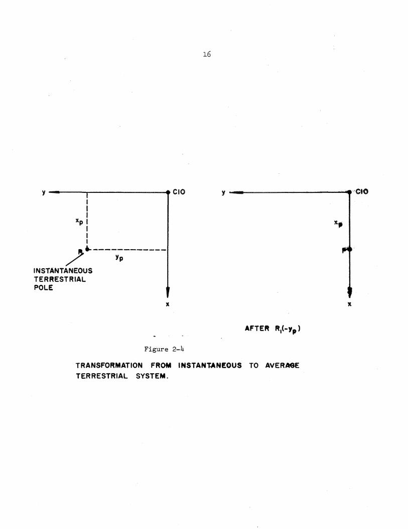
y -.....---,--------• CIO I I I
"P I I I I
~~---~p-------INSTANTANEOUS TERRESTRIAL POLE
X
Figure 2-4
16
y -~-----------•, .. CtO
TRANSFORMATION FROM INSTANTANEOUS TO AVERAGE TERRESTRIAL SYSTEM.

17
where (x , y } are expressed in arcseconds, and the rotation matrices p p
are
1 0 0
Rl (-yp) = 0 cos{-y ) sin(-y ) p p
0 -sin(-y ) cos(-y ) p p
a clockwise (negative) rotation about the x axis, and
cos(-x ) 0 -sin(-x } p p
R2 (-xp) = 0 1 0
sin(-x } 0 cos(-x } p p
a clockwise (negative) rotation about they-axis. The inverse is
X X
y
z I.T. z A.T.
and because of the orthogonal characteristic of rotation matrices, that is
-1 T R (a) = R (a) = R (-e)
X X
y y • 2-3
z I.T. z A.T.
2.1.3 Geodetic Systems
In terms of Cartesian coordinates, the geodetic (G) coordinate
system is that system which is introduced into the earth such that its
three axes are coincident with or parallel to the corresponding three

18
axes of the average terrestrial system (see Figure 2-3). The first
situation defines a geocentric geodetic system while the latter non-
geocentric system is commonly referred to as a relative geodetic s~stem,
whose relationship to the average terrestrial systeo is given by the
three datum translation components
r = 0
X 0
z 0
and in vector equation form, the relationship is
Ri = ro + ri
where the position vector ri is referred to the geodetic system, that is
and·
X
y = z A.T.
X
y
z
X 0
z 0
G
X
2-4
z G
A more detailed account of how a relative geodetic system is
established within the earth is in order {Section 2.3),but before this
can be done, it would be useful to review the relationship between
Cartesian and curvilinear coordinates.

19
2. 2 RELATIONSHIP BETWEEN CARTESIAN AliD CURVILINEAR COORDIIIATES
In this section we first describe the Cartesian (x, y, z) and
curvilinear (latitude, longitude, height) coordinates for a point ·on the
reference ellipsoid. We then develop expressions for its position
vector in terms of various latitudes. Finally the transfOrmation tram
geodetic coordinates (41, A:, h) to (x, y, .z) and its inverse are
discussed.
2.2.1 Cartesian and Curvilinear Coordinates of a Point
on the Reference Ellipsoid
. The specific ellipsoid used in geodesy as a reference surface is
a rotational ellipsoid formed from the rotation of an ·e~ipse about its
semi-minor axis b (Figure 2-5). The semi-ma.lor axis a and -the
flattening
f = .;;;;a~-_b;;. a
are the defining parameters of the reference ellipsoid.
2-5
Other useful parameters associated with this particular ellipsoid
are the first eccentricity
2 e =
'
and the second eccentricity
2-7
A Cartesian coordinate system is superimposed on the reference
ellipsoid (see Figure 2-5) so that:

20
i!
Figure 2-5. REFERENCE ELLIPSOID

21
a) The origin of the Cartesian system is the centre of the
ellipsoid.
b) The primary pole (z-axis) of the Cartesian system is the
semi-minor axis of the ellipsoid. The primary plane is perpendicular
to the primary axis and is called the equatorial plane.
· c) Any plane containing the semi-minor axis and cutting
the surface of the ellipsoid is called a meridian plane. The particular
meridian plane chosen as the secondary plane is called the Greenwich
meridian plane. The secondary pole (x-axis) is the intersection of
the equatorial plane and the Greenwich meridian plane.
d) The y-axis is chosen to form a right-handed system, and
lies in the equatorial plane, 90° counterclockwise from the x-axis.
The equation of this ellipsoid, in terms of Cartesian coordinates
is
1? s E x = 1 ' 2-8
where
-T (x y z] X = '
l/a2 0 0
SE = 0 l/a2 0 '
2-9
0 0 l/b2
or
x2 + Y2 2 + z
1 = • 2 b2 a 2-10
The latitude of a point is the acute angular distance between the
equatorial plane and the ellipsoid normal through the point measured in
the meridian plane of the point. The line perpendicular to the ellipsoid
at a point is called

22
the ellipsoid normal at the point. Ellipsoid normals only pass through
the geometric center of the ellipsoid in the equatorial plane or along
the semi-minor axis. Therefore there are two different kinds of
latitude. The angle between the ellipsoid normal at the point and the
equatorial plane is called the geodetic latitude ~. The angle between
the line joining the point to the centre of the ellipse, and the
equatorial plane is called the geocentric latitude ~- There is also a
third latitude, used mostly as a mathematical convenience, called the
reduced latitude 6 (see Figure 2-6).
The longitude A of a meridian plane is the counterclockwise angular
distance between the Greenwich meridian plane and the meridian plane of
the point, measured in the equatorial plane (see Figure 2-5).
The ellipsoid height h of a point is its linear distance above the
ellipsoid, measured along the ellipsoidal normal at the point (see Figure 2-8}.
2.2.2 The Position Vector in Terms of the Geodetic Latitude
Consider a point P on the surface of the ellipsoid. The coordinates
of P referred to a system with the primary axis (denoted x*) in the meridian
plane of P are
r = 0 2-11
Zj
The plane perpendicular to the ellipsoid normal at P, and passing
through P is called the tangent plane at P. From Figure 2-7 the slope
of the t.angent plane is
dz dx*
cosp sinljl 2-12

0
b
23
a
V GEOCENTRIC LATITUDE
+ GEODETIC LATIYI"uVE .. . .
/J REDUCED LATITOOE
P ACTUAL POINT
Q,R PROJECTED POINTS
Figure 2-6. VARIOUS LATITUDES . .

24
• p
Figure 2-T. TANGENT LINE TO THE MERIDIAN ELLIPSE

25
The slope can also be computed from the equation of the meridian ellipse
as follows:
or
b2 ( *)2 2 2 2 b2 x +a z =a
dz 2 b x* dx* = - 2
a z
It follows from·~he above two equations for the slope, that 2 .
b x* _ cos; 2 -
a z sin~ or
b1 (x*) sin ~ = a1 z cos ~
and after squaring the above
4 2 . 2 4 2 2 b (x*) s~n ~ = a z cos ~
Expressing equations 2-14 and 2-19 in matrix form
The inverse of the coefficient matrix is
1
a 2 2(a2 2 2 2 ) o cos 4>·+ b sin ~
[ a2
-b2
1 [a4 cos2~]
2 2~ b2 . 2~ 4 2 a cos ~ + s~n ~ b sin $
and finding the square root
[x*J 1 z = (a2 cos2~ + b2 . 2~)1/2
s~n "'.
2-13
2-14
2-15
2-16
2-17
2-18
2-19
. 2-20
2-21

~·rom Figure 2-6
but from equation 2-21
therefore
r =
cos x* ¢." =
N
2 a cos$ x* = --~~~~~----------~-2 2 2 n , jn
( • • .::; ) .i.{ t::. a cos ~ + o sin ~
2 N = ------~a~-------------
x*
0
z
( 2 2~ b2 . 2~)1/2 a cos i' + s1.n 'I'
= r N :os$ L N b2 /a2 sin$
2-22
2-23
N is the radius of curvature of the ellipsoid surface in the plane
perpendicular to the meridian plane (called the Prime vertical plane).
We now refer the position vector P to a system with the primary axis
in the Greenwich meridian plane, that is we rotate the coordinate system
about the z-axis clockwise (negative rotation) through the longitude A.
X x*
r = y = R3(->.) 0
z z
cos(->.) sin(->..) 0 N cos4>
= -sin(->.) cos(-/c) 0 0
0 0 1 N b2/a 2
sin4>

27
or
X cos' COSA
r = y = N cos' sinA 2-24
z b2/a2 sin'
2.2.3 The Position'Vector in Terms of the Geocentric and Reduced Latitudes
From Figure 2-6 the position vector of the point P in terms of the
geocentric latitude ~ is
x* ·cos~
r = 0 = lrl 0
z sin~
where lrl is the magnitude of r.
Rotating the coordinate system to introduce longitude as before,
X
r= y
z
x*
0
z
= lrl
cos~ cosA
cos~ sinA
sin~
2-25
From Figure 2-6 the reduced latitude 8 of the point P is the
geocentric latitude of both the points Q and R, where Q is the
projection of P parallel to the semi-minor axis to intersect a circle
with radius equal to the semi-major axis, and R is the projection of the
point P parallel to the semi-major axis to intersect a circle with
radius equal to the semi-minor axis.
The position vector of P in terms of the reduced latitude 8 is
x* a cos8
r= 0 = 0
z b sinS·

28
Rotating the coordinate system to introduce longitunes
X x* a case COSA
r = y = R3(-A.) 0 = a case sin>.. 2-26
z z b sine
2.2.4 Relationships between Geodetic, Geocentric and Reduced Latitudes
From equations 2-24, 2-25, and 2-26
z - = X
b tan$ cosA. =tan~ cosA. =-tanS cosA.. a
Cancelling the cos A. term,
tanS b
tan$ =-r ' a
tanS a tamjl = ' b
tantjl b2
=- tancjl . 2 a
2-27
2-28
2.2.5 The_Position Vector of a Point Above the Reference Ellipsoid
Let us consider a terrain point i, as depicted in Figure 2-8,
whose coordinates are the geodetic latitude $ and longitude >.., and
the ellipsoid height h. The projection of i onto the surface of the
ellipsoid is along the ellipsoidal normal defined by the unit vector
The position vector of i is then the sum of two vectors, namely
r. = r + h u 1. p z s 2-30
u • z
where r is defined by equation 2-24 and u is the unit vector defined p z
by equation 2-68c, that is

29
TERRAIN POINT
Figure 2-8. POINT ABOVE REFERENCE ELLIPSOtO
30
COS$ COSA
U = COS$ SinA z
sin$
Thus
X cos$ COSA cos$ COSA
ri = y = N cos$ sinA. + h cos$ sinA.
z b2/a2 sin$ sin$
or
~
(N+h) cos$ -COSA
= (N+h) cos$ sinA. 2-31
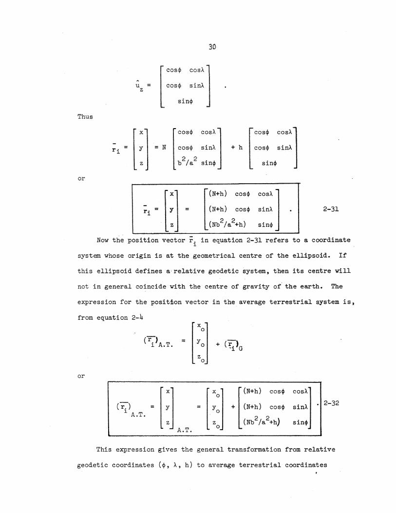
z sin$ I. - --Now the position vector r. in equation 2-31 refers to a coordinate
1
system whose origin is at the geometrical centre of the ellipsoid. If
this ellipsoid defines a·relative geodetic system, then its centre will
not in general coincide with the centre of gravity of. the earth. The
expression for the position vector in the average terrestrial system is,
from equation 2-4
(ri)A.T. =
or
X
cr.> = 1 A.T.
y
z
X 0
z 0
=
+ ("I\) 'l. G
X 0
z 0
(N+h) cos$ COSA
+ (N+h) cos$ sinA.
(Nb2/a2+h) sin$
• 2-32
This expression gives the general transformation from relative
geodetic coordinates ($, A., h) to average terrestrial coordinates
31
(x, y, z), given the size of the ellipsoid (a, b) and the translation
components (x y z ) o' o' o •
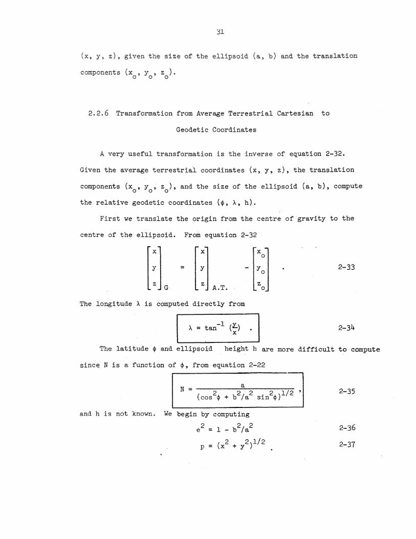
2.2.6 Transformation from Average Terrestrial Cartesian to
Geodetic Coordinates
A very useful transformation is the inverse of equation 2-32.
Given the average terrestrial coordinates (x, y, z), the translation
components (x , y , z ), and the size of the ellipsoid (a, b), compute 0 0 0
the relative geodetic coordinates (,, A, h).
First we translate the origin from the centre of gravity to the
centre of the ellipsoid. From equation 2-32
X X
y = y
z G
z A.T.
The longitude A is computed directly from
X 0
z 0
X = tan-l (~) ·I
2-33
2-34
The latitude ' and ellipsoid height h are more difficult to compute
sine~ N is a function of~. from equation 2-22
and h is not known. We begin by computing
e 2 = 1 - b2/a2
( 2 2)1/2 p = X + y
2-35
2-36
2-37

From equation 2-31
2 p =
p = or
Also from 2-31
Therefore z - = p
(N+h)
I
32
cos<P
p J h = coscj> - N
z = (N b2/a2 + h)
a2-b2 = (N - 2 N a
= (N + h - e 2 N)
+ h) sin$
sincfl .
(N·+ h-e~) sinp _ t (l e~) - ancf! --(N + h) coslj> N+h
2-38
2-39
This equation can be developed in two wayss to produce either a direct
solution for 4> which is quite involved, or an iterative solution which is
simpler. We consider the iterative solution first. We have
Each
0 = tan-1 [<~) (1 - ;~) - 1] •
The iterative procedure is initiated by setting
iteration then
N. = J.
hi =
N = a 0
consists
2 cos <fl. 1
J.-
E
cosq,i-l
of evaluating in order
a
+ b2/a2 . 2q, )1/2 s1.n . 1 1.-
~ N. 1.
2 eN. )-1] -1 [t· cj>i = tan p) (1- 1. . N.+h.
J. J.
and
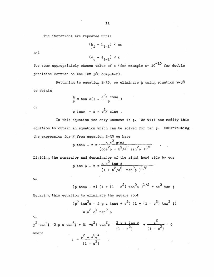
33
The iterations are repeated until
(h. - h. 1) < 8£ l. l.-
..:.10 for some appropriately chosen value of E (for example E= 10 for double
precision Fortran on the IBM 360 computer).
Returning to equation 2-39, we eliminate h using equation 2-38
to obtain
.!. = tan ~(l _ e~ cosp ) p p
or p tan~ - z = e~ sin~ •
In this equation the only unknown is $. We will now modify this
equation to obtain an equation which can be solved for tan $. Substituting
the expression for·N from equation 2-35 we have
a e2 sinp
Dividing the numerator and denominator of the right hand side by cos 2
p tan ~ - z = .;;;a.....;..e_t.-a.n~-4>~-~~~~-(1 + b2/a2 tan2~ )l/2
or
2 ae tan ~
Squaring this equation to eliminate the square root
(p2 tan2~ - ~ p z tan~ + z2 ) (1 + (l - e2 ) tan2 ~) 2 4 2 = a e tan <f;
or
2 4 3 2 2 p tan ~ -2 p z tan ~ + (3 +z ) tan ~
2 + ---'-z __ = 0
(l - e 2 ) where
3 -

34
This is a quartic (biquadratic) equation in tan' , in which the
values of all coefficients are knowh. Standard procedures for solving
quartic equations exist (see for example Kern and Kern, 1968), and have
been applied to this equation by Paul (1973), to prod~ce a computer
program which is about 25% faster than iterative programs. Once a solution
for tan~ is obtained, N and h are computed from equations 2-35 and 2-38
respectively.
2.3 GEODETIC DATUMS
There are two natural figures of the earth (see Figure 2-9);
the topographic or physical surface of the earth including the surface of
the oceans (the terrain), and the equipotential surface of the earth's
gravity field which coincides with an idealized surface of the oceans (the
geoid}.
Control measurements (e.g. distances, angles, spirit levelling)
are made between points on the terrain which we call control points. These
measurements are used to determine the geometrical relationship between
the control points in a computation called network adjustment. Other points
are then related to the network of control points through further measurements
and computations called densification. The classical approach is to treat
the vertical measurements, networks and computations aeparately from the
horizontal measurements, networks and computations. However the unified
three dimensional approach is currently gaining favour. {Hotine, 1969].
In the classical approach vertical measurements·and networks are
referred to a coordinate surface or (vertical) datum which is th~ geoid.
Rather than using the geoid as the coqrdinate surface or datum for the
horizontal measurements and networks as well, a third, unnatural figure of

AXIS OF EARTH
CENTRE OF
AXIS OF ELLIPSOID
34A
--~= -~ DEFL~CTI~N OF J ~ THE VERT-ICAL
ELUPSOID.,_-~.._-¥-______ .__.......;. __ ....,._
CENTRE OF GRAVITY
LATITUDE~
Figure 2-9. _ MERIOlAN SECTION -OF TH£ E·ARTH
35
the earth is introduced - the ellipsoid of rotation discussed earlier.
The reason a mathematical figure like the ellipsoid is used as the horizontal
~ is to simplify the computations required both for network adjustment
and densification.
Correction terms are necessary in these computation to account
for the fact that the datum is not the geoid. An ellipsoid can be chosen
to approximate the geoid closely enough that.these correction terms can
be assumed linear and for some applications even ignored. For a well-chosen
ellipsoid (see Figure 2-9), the geoid-ellipsoid.separation (geoid height)
is always less than 100 metres, and the difference between the geoid and
ellipsoid normals at any point (deflection of the vertical) is usually le~s
than 5 arc seconds, very rarely exceeding 1 arcminute.
Even simpler surfaces than the ellipsoid (such· as the sphere
or the plane} can be sufficient approximationsoto the.geoid if the area
under consideration is sufficiently small, and/or the control application
permits lower orders of accuracy.
s The introduction of a new surface (the ellipsoid) has a price.
The horizontal control network (that is .. the coordinates of the points of the
network) is to be referred t? the eilipsoid. Therefore before network
computations can begin, the control measurements must first be reduced so
that they too "refer" to the ellipsoid.
It is important to distinguish between the datum (the coordinate
surface or ellipsoid surface) and the coordinates of the points of the net-
work referred to the datum. It is a common but confusi_ng practice (part
icularly in North.America) to use the term "datum" for the set of coordinates.

36
2.3.1 Datum Position Parameters
In order to establish an· ellipsoid as the reference surface for
a system of control we must specify its size and shape (usually by assigning
values to the semi-major axis and flattening) and we must specify its pos
ition with respect to the ea1;th. A well~positioned ellipsoid will closely
approximate the geoid over the area covered by the network for which it is
in datum. The parameters to vhich we assign values in order to specify the
ellipsoid position we call the datum position parame;;ers.;·
In three-dimensional space~ any figure {and particularly our
ellipsoid) has six degrees of freedom~ that is six ways in vhich its posi
tion with respect to a fixed figure (in our case the earth) can be changed.
Thus there are -six datum position parameters.
Another vay of looking at this is to consider tvo three-dimensional
Cartesian coordinate systems, one fixed to the ellipsoid and one fixed to
the earth. In general the origins of the two systems will not coincide,
and the axes vill not be parallel. Therefore, to define the transformation
from one system to the other we must specify the location of one origin
with respect to the other system, and the orientation of one set of axes
with respect to the other system, that is three coordinates, and three
rotation angles. These six parameters provide a description of the six
degrees of freedom and _assigning values to them positions the ellipsoid
with respect to the earth. They are our six datum position parameters. A
datum then is completely specified by assigning values to eight parameters
the ellipsoid size and shape, and the six datum position parameters.

37
There are in fact two kinds of datum position parameters in
use. One kind is obtained by considering the ellipsoid-fixed and earth-. >v.·
fixed coordinate systems to have their origins in the neighbourhood of the
geocentre. The other kind is obtained by considering the ellipsoid-fixed
and earth-fixed coordinate systems to have their origins near the surface
of the earth at a point we call the initial point of the datum.
In the first (geocentric) case the earth-fixed system is the
Average Terrestrial system of section 2.1.2, and the ellipsoid-fixed system
is the geodetic system of Equation 2-31 (except that here we assume the
geodetic and average terrestrial axes are not in general parallel). In
this case the datum position parameters are tne Average Terrestrial coor-
dinat.es ·of the ellipsoid origin (x , y , z of Equation 2-32} and three 0 0 0
rotation angles (say w1 , w2 , w3 ) required to define the misalignment bet-
ween the axes. It is of course highly desirable that the ellipsoid be
positioned so that these angles are as small as possible, particularly
that the two axes of symmetry (the ellipsoid minor axis and earth's average
rotation axis or Average Terrestrial z-.axis) be parallel.
In the second (topocentric) case the earth-fixed system is a
local astronomic system at the initial point, and the ellipsoid-fixed
system is a local geodetic system at the same point (local astronomic and
geodetic systems are discussed in section 2.4).
Before proceeding further let us consider the geometry in the
neighbourhood of a point on the earth's surface. Figure 2-10 is an exag-
gerated view of the geodetic meridian plane at such a point, showing the
sectioned ellipsoid, geoid, several equipotential surfaces related to the
geoid, and the terrain. A particular ellipsoid normal intersects the

37A
SUR.F,\c:E GaRA\I•TY VE(TICAt..
FIGURE 2-10
ORIENTATION OF ELLIPSOID TO GEOID
EQUIPOTENTIAL. SURFACES

38
ellipsoid, geoid, and terrain at Q,P and T respectb·ely. There are three
"natural" normals corresponding to this ellipsoid normal; the surface
gravity vertical (perpendicular to the equipotential surface at T, passing
through T) , the geoid gravity vertical (perpendicular to the geoid pass_ing
through P), and the plumbline (perpendicular to all equipotential surfaces
between terrain and· geoid, passing through T}. In general, the plumbline
is curved while the others are straight lines, and none of these three
actually lie in the geodetic meridian plane - they are shown here as pro-
jections onto this plane. If the curvature of the plumbline is ignored
the two gravity verticals are parallel.
The astronomic meridian plane is the plane containing one of
the gravity verticals and a parallel to the Average Terrestrial z-axis.
The angle between the gravity vertical and the parallel to the A.T •. z-axis
i.s the astronomic co-latitude <; - t). The angle between the astronomic
meridian plane and a reference meridian plane (Greenwich) is the astronomic
longitude A. The angle between the ellipsoid normal and the gravity
vertical is the deflection of the vertical, which can be resolved into a
component ~ in the geodetic meridian plane and a component n in the
geodetic prime vertical plane (the plane perpendicular to the geodetic mer-
idian plane which contains the ellipsoid normal). Thus corresponding to
the two gravity verticals, there are two sets of values for the astrqnomic
latitude and longitude and deflection components, and if the curvature of
the plumbline is ignored, these two sets are equal.
If the ellipsoid is positioned so that itE geocentric axes are
paralled to the Average Terrestrial axes (that is w1
n = (A -A) cos ~
= w = w = 0) then 2 3
2-40
2-41

39
where ($, A) are the common geodetic coordinates of Q~ P. and T.
The distance between the ellipsoid and geoid, measured along
the ellipsoid normal (QP) is the geoid height N*. The distance between the
ellipsoid and terrain, measured along the ellipsoid normal (QT.} is the
ellipsoid height h. The distance between the geoid and terrain, measured
along the plumbline (P'T) is the orthometric height H. If the curvature
of the plumbline is ignored
h = N* + H.
Given a point some distance from T, the angle between the geodetic
meridian plane and the plane containing this point and the ellipsoid ndriaa.J.
QPT is the geodetic azimuth a ·of that point with respect to Q, P or T.
(Actually this is the azimuth of the normal section, and is related to the
geodetic azimuth by small corrections ( Bamford, 1971)}. The angle betweenthe
astronomic meridian plane and the plane containing this point and the cor
responding gravity vertical is the astronomic azimuth A of that point with
respect to either P or T depending on which gravity vertical is used.
Because the deflection of the vertical is small, then for all such points
the difference
oa = A -a 2-43
is nearly constant, and is the angle between the geodetic and astronomic
meridian planes.
Returning to the topocentric datum position parameters, it is
natural to specify that our local geodetic system at the initial point have
its origin on the datum surface, that is on the ellipsoid. In the classical
(non-three-dimensional) approach the orthometric height H enters into hori
zontal networks only in the reduction of surface quantities to the geoid,

40
therefore it is natural to take our local astronomic system at the initial
point to have its origin on the g~oid. Denoting quantities at the initial
point by a zero subscript, we. then see that the six datum position para
meters are in this case the geodetic coordinates of the local astronomic
origin (q, , :A ·, N*) and the rotation angles required to define the trans-0. 0 0
formation between the local geodetic and local astronomic systems (~ , n , . 0 0
oa ) . 0
2.3.2 Establishment of a Datum
We have seen that a datum is defined by assigning values either
to the eight parameters (a, b, x0 , y0 , z0 , w1 , w2 , w3 ) or to the eight
parameters (a, b, q,0 , A0 , N*0 , ~0 , n0 , oa0 ). However, an arbitrary set
of values will not in general result in a satisfactory datum~ We recall
that it is important that a datum closely approximate the geoid over the
area of the network for which it is a datum, and that the geocentric axes
of the geodetic .coordinate system be closely parallel
to the Average Terrestrial axes, particularly that the axes of symmetry be
parallel. The process of assigning values to the eight datum parameters in
such a way that these characteristics are obtained is called establishment
of a datum.
To begin with, in establishing a datum values are always assigned
to the topocentric set (a, b, 4> ,A , N* , ~ , n , oa ) rather than the geo~ 0 0 0 0 0 0
centric set (a, b, x 0 , y0 , z0 , w1 , w2 , w3 ) because it is the set which is
related to the geodetic and astronomic measurements which we must use in
establishing the datum. We see that we must somehow choose values for
(a, b, q,, A, N*, ~, n0 , oa0 ) so that the values of (N*,~,n) elsewhere 0 0 0 0

in the network are not excessive (the datum approximates the geoid), and
so that w1 = w2= w3= 0 (the axes are parallel). Additionally ror networks
of global extent we require that x = y = z = 0, in which case the datum 0 0 0 .
is termed a geocentric datum. Otherwise the datum is a local datum.
The problem of approximating the geoid can be ignored, in which
case the values
N* = ~ = n = o 0 0 0
are assigned, which rorces the ellipsoid to intersect and be tangent to the
geoid at the initial point.
The geoid can be approximated in two ways, by choosing values
of (a, b, N*0 , ~0 , n0 } such that either values of (~, n) or values or N*
throughout the network are minimized (Vanicek, 1972). Note that values
of (N*, ~. n) are available throughout the network only ir some adjusted
network already exists, which points up the iterative nature or datum
establishment - a "best ritting" datum can be established only as an improve
ment on an already existing datum.
The classical method of' "ensuring" that the axes of' symmetry
are parallel is to enforce the Laplace azimuth condition at the initial
point, that is to assign a value to a according to 0
oa = A - a = n tan ~ 0 0 0 0 0
2-44
where A is an observed astronomic azimuth. This condition forces the 0
geodetic and astronomic meridians to be parallel at the initial point, and
thus forces both axes of' symmetry to ·,lie in this corJmon plane. However,
the axes of' symmetry can still be misaligned within the meridian plane.
The solution to this dilemma has been to apply the Laplace condition at
several geodetic. meridians parallel to their corresponding astron6mic
42
meridians. In essence this constrains the adjusted network to compensate
for misalignment of the datum, rather than ensuring that the datum minor
axis is parallel to the earth's rotation axis. Note that enforcing the
Laplace condition throughout the network presumes th~ existance of an
adjusted network, which again _points up the iterative nature of datum
establishment.
2.3.3 The North American Datum
The iterative nature of datum establishreent is illustrated by
the history of the North American Datum.
Towards the close of the last century geodetic networks existed
in several parts of North America, each defined on its c~ datum. The
largest of these was the New England Datum established in 1879 with an
initial point at Principia, Maryland. The New England Datum used the Clarke
1866 ellipsoid, still used by the North American Datum today.
By 1899 the U.S. Transcontinental Network linking the Atlantic
and Pacific coasts was complete. When an attempt was made to join the neWer
networks to those of the New England Datum large discrepancies occurred.
Therefore in 1901 the United States Standard Datum was established. The
Clarke 1866 ellipsoid was retained from the New England Datum, but the
initial point was moved from Principio to the approximate geographical centre
of the U.S. at Meades Ranch, Kansas. The coordinates ruid azimuth at Meades
Ranch were selected so as to cause minimum change in existing coordinates
and publications (mainly in New England) while providiP.g a better fit to
the geoid for the rest of the continent.

43
Meanwhile additional networks were being established in the
United States, Canada and Mexico. In 1913 Canada an~. Mexico agreed to
accept Meades Ranch as the initial point tor all North American networks,
and the datum was renamed the North American Datum.
This eventually led to the readjustment, between 1927 and 1932,
of all the North American networks then in existance. The 1901 coordinates
of Meades Ranch and the Clarke 1866 ellipsoid remained unchanged, however
the value of the geodetic azimuth was changed by abo~t 5 arcseconds {Mitchell,
1948). Thus the new datum was called the 1927 North American Datum.
~ definition of the North American Datum was not yet complete. It
was only in 1948 that astronomic coordinates were observed at Meades Ranch,
allowing specification of values tor ~ , 11 • The final datum parameter 0 0
was defined in 1967 when the U.S. Army Map Service chose a value of N' = 0 0
at Meades Ranch tor their astrogeodetic geoid [Fischer, et al 1967]. Table
2-1 lists the values assigned to the datum parameters for the North American
Datum, and the date at which they were determined.
Since the 1927 readjustment many new networks have been added
to what was then available. However, these new networks have been adjusted
by "tacking them on~' to· previously adjusted networks, ,.the latter being held
fixed in the process. Until the recent advent of large fast digital computers
it was impractical to consider readjusting all the networks on the continent
again, consequently distortions have crept in to the networks, a notorious
case being the 10 metres discrepancy which has been "drowned" in Lake Superior
by international agreement. The day is fast approaching when a massive new
readjustment and perhaps redefinition of the North American Da.tum ·will occur
[Smith, 1971]. One landmark on this path is the International Symposium on
Problems Related to the Redefinition of North American Geodetic Networks,

44
Table 2-1
PARAMETERS DEFINING THE
1927 NORTH AMERICAN DATUM
Clarke 1866 Ellipsoid semi-major axis a = 6378206.4 metr.es.
Clarke 1866 Ellipsoid semi-minor axis b = 6356583.8 metr~s
Initial Point Latitude of Meade's Ranch 41 = 39° 13' 26".686 N 0
Initial Point Longitude of Meade's Ranch A = 98° 32' 30".506 W 0
Initial Point Azimuth (to Waldo) 75° 28' 9".64
Date Ado;eted
} 1879
1 -+<
1901
a .= 0~ {clockwlse from south} 1927
Initial Point Meridian Deflection Component ~ = -1.02" } 0
Initial Point Prime Vertical 1948
Deflection Component n = -1. 79" 0
Initial Point.Geoid Height N.~t = 0 1967 0
Table 2-2
TRANSLATION COMPONENTS
X yo z a a a 0 :0 xo· yo . zo
Merry & Vanicek -28.7 150.5 179-9 1.7 1.0 1.2
Krakiwsky et al. -35 164 186 2 3 3

May 1974 at the University or New Brunswick.
The North American Datum is a local datums that is its geo-
metrical centre does not coincide with the origin of the Average Terres-
trial system. Because of the distortions in the networks just mentioneds
determinations of x , y , z vary depending on the locations at which 0 0 0
they are measured. Two recent sets of values obtained by different methods
are listed in Table 2-2. Merry and Vanicek [1973] used data within 1000
km of Heades Ranch. Krakiwsky et al [1973] used data from New Brunswick
and Nova Scotia. The discrepancies of order 10 metres likely reflect the
distortions which exist in the present North American networks.
2.3.4 Datum Transformations
If the curvilinear coordinates of an observing station referring
to one particular datum are given, then a problem which often occurs is to
obtain the curvilinear coordinates for the station referred to another datum.
In transforming coordinates from one datum to another it is
necessary to account for two items:
a) the location of the geometric centres of each reference
ellipsoid with respect to the centre of gravity of the earths or with
respect to each other,
b) the difference in size and shape between the ellipsoids.
It is usually assumed that the axes of both datums are parallel to the axes
of the average terrestrial system.
Consider the ellipsoids with sizes and shapes defined by (a1 ,b1 )
and (a2 ,b2 ) (or alternatively (a1 , f 1 ) .and (a1 ,f2 ), where f=(a-b)/a)and with
locations of the geometric centres with respect to the centre of gravity
defined by

and
( - ' r i~ 0 j_
cr: ) 0 2
46
= r~:J, L z -
0 .J.
X 0
= Yo
z 0 r. c.
Let us define the coordinates of a point referred to the first
ellipsoid as ( ~l, >.. 1 , h1 ). We want to find the coordinates of the
same point, referred to the second ellipsoid {~ 2 , >.. 2 , h2 ).
The average terrestrial coordLnates of the point are given by
equation 2-32:
X X (Nl + hl) cos..P1 CO SAl 0
y = Yo + (N + h1 ) cos$1 sinA.1 • 2-45 l 2 2
hl) z (N1 b/a1 + sin..p1 l
But the average terrestrial coordinates are not affected by a
X X (N2 + h2) cos$2 COSA2 0
y = yo + (N2 + h2) cos..p2 sinA.2 2-46
(N2 2, 2
h ) sin$2 z A.T. z b2;a2 + 0 z 2
There are two methods for obtainiP~ (..p 2 , >.. 2 , h2 ). The first
method, called the iterative method is to find the average terrestrial
coordinates directly from equation 2-45, and then to invert equation
2-46 to find (..p 2 , >.. 2 , h2 ), using the iterative method described in
section 2.2.6.

47
The second method, called the differential method can be applied
when the parameter differences (oa, of, ox ' oy ' oz ) between the two datums 0 0 0
is small enough that we can use the Taylor's series linear approximation.
Taking the total differential of equation 2032, keeping the average terres-
trial coordinates invariant, and setting the differential quantities equal
to differences between the datums we have
where
Solving
where
J =
B =
ox 0
oy 0
ox 0
- (M+h)
(M+h)
(M+h)
li coscp
N cos'
+ J
oh
sin' COSA , -
sin~ sinA.,
cos~ ,
cos>./a ' sin>./a
' N (l-f) 2 sincp/a >
f4 = 2 2 2 a(l-f) /(cos <P + (1-f)
for the coordinate differences
o<J>
I a>. -1 = -J
oh
+ B [::] = 0
(N+h) cos~ sinA. '
cos~ COSA
(N+h) cos~ cos>. cos~ sin>.
0 ) sin ~
M . 2~ s~n cos~ cosA./(1-f)
M . 2~ s~n cos~ sinA/(1-f)
(M sin2<J> - 2N) sincp (1-f)
. 2<jl)3/2 s~n
o.x [::] 0
oy + B 0
oz 0
[- sinf cos>../ (M+h) , - sin~ sinA./(M+h) ·~ cos,/(M+h)
-1 - sin>./ (N+h) cos<jl ' cos>./ (N+h) cos~ ~ 0 J = cos~ COSA ' coscp sin). , sin <I>
2-47
2-48
2-49
2-50
2-51
2-52

48
Note that the matrices can be evaluated in either of the two coordinate
systems, since the differences in quantities has been assumed small. Further
it is reasonable to simplify the evaluation of the matrices by using the
spherical approximation (f = 0, H = M = N+h = M+h = a) in which case ve
obtain the transformation equations of Heiskanen and Moritz (1967, equation
5-55).
Table 2-3 shows an example of datum transformation computations.
This particular example transforms the coordinates of a station in Dartmouth,
Nova Scotia froi!l the 1927 North American Datum ("Old"Datum) to the 1950
European Datum ("New" Datum). The datum translation components used are
those given by Lambeck [1971). Both the iterative method of equations
2-45 and 2-46, and the differential method of equation 2-51 were used. The
discrepancies between the two results are about 0.4 meters in latitude,
0.3 meters in longitude, and 0.2 meters in height.
2.4 TERRESTRIAL TOPOCENTRIC SYSTEMS
In the introduction it was stated that terrestrial topocentric
systems are defined as follows:
a) the origin is at a point near the surface of the earth,
b) the primary plane is the plane tangential to the earth's
surface at the point,
c) the primary axis is the north point,
d) the systems are left-handed.
The last two specifications present no problem!:. However, "the
surface of the earth" can be interpreted in three ways to mean the
earth's physical surface, the earth's equipotential surface, or the

Table 2-3.
EXAMPLE OF DATUM TRANSFORMATIONS
Parameter "Old" Datum "New" Datum "New'~-"Old"
r
Given:
semi-major axis a 6378206.4 meters 6378388.0 181.6
flattening f 1/294-98 1/297-0 -5 -2-30,Tno
{:: -25.8 -64.5 -38.7
o ffset from geocentre 168.1 -154.8 -322.9 (from Lambeck [1971])
167.3 -46.2 -213.5
cl 44.683°N ?
observer's coordinates Al 63.612°W ?
hl 37.46 meters ? .
Solution b:t: Iterative Method:
{: 2018917.91 2018917.91
observer's coordinates -4069107.35 -40691·07. 35 in average Terrestrial 4462360.64 4462360.64 System (Equation2-45)
{ lj>l 44.6847lQ0 N
observer's coordinates A_t 63.609752°W (Equation 2-46)
h2. -259-U meters
Solution b:t: differential Method:
change in semi-major axis cSa 181.6
change in flattening of -2.3057xlo-5
change in offsets from r· -38.7 geocenter cSy: -322.9
oz -213.5 . 0
observer's coordinates
{ q,2 44.6841Q.6°N
(Equation 2-50). ).2 63.6097~0W
h2 -259. ,2g, meters

50
surface of a reference ellipsoid. It is not practical to define a
coordinate system in terms of a planetangential to the earth's physical
surface. Two kinds of terrestrial topocentric coordinate systems can
be defined, however~ The system in which the primery pole is the
normal to the equipotential surface at the observation station is
called a local astronomic system; The system in which the primary
pole is the ellipsoid normal passing through the observation station
is called a locai geodetic system [Krakiwsky 1968].
2.4.1 Local Astronomic System
A local astronomic (L.A.) system is speciried:
a} The origin is at the observation station.
b) The primary pole (z-axis) is the normal to the equipo-
tential surface (the gravity vertical) at the observation station. The
primary plane is the plane containing the origin and perpendicular to
the gravity vertical.
c) The primary axis (x-axis) is the intersection of the
primary plane and the plane containing the average terrestrial pole and
the observation station, and is called the astronomic north.
d) The y-axis is directed east to form a left-handed system.
The position vector of an observed station 1, expressed in the
local astronomic system of the observation station k, is given by
X cos vtl cos ~1 (rkl)L.A. = y = rkl cos vtl sin ~ 2-54
z . v L.A. s~n kl
51
z
ELLIPSOID PARALLEL TO NORMAL THE AVERAGE ROTATION AXIS x NORTH
PARALLEL TO THE GREENWICH MEAN MERIDIAN
X
z
MERIDIAN
·.,
Figilre 2-12
GEODETIC AND LOCAL GEODETIC COORDINATE SYSTEMS
y
EAST
;

52
where rkl is the terrestrial spatial distance, vkl the vertical angle,
and ~1 the astronomic azimuth.
Note that the relationship of the local astronomic system to the
average terrestrial system is given by the astronomic latitude ~k and
longitude Ak only after the observed quantities ~k' Ak, ~l have been
corrected for polar motion •. Thus the position vector rkl of 2-54
expressed in the average terrestrial system is:
X X
y = y 2-55
z A.T. z L.A.
vhere the reflection matrix
1 0 0
0 -1 0 2-56
0 0 1
accomplishes the transformation from a left-handed system into a right-
handed system, while the rotation matrices
cos (90':.~k) 0 -sin (90-~k)
R2 = 0 1 0 2-57
sin ( 90.._\) 0 cos (9rf-~k)
and
cos(l~O:_Ak) sin(l8o:.Ak) 0
R3 = -sin(lBo-Ak) cos ( 18o'1-Ak) 0 2-58
0 0 1
. bring the three axes of the local astronomic systeiD parallel to the
corresponding axes in the average terrestrial system.
The inverse transformation is

53
" 2-60
Note that so far no translation!; have taken place. We have merely
rotated the position vector (rk1 ) of station 1 with respect to station
k into the average terrestrial system. If the position vector of
station k with respect to the centre of gravity in the average
terrestrial system is{Rk)A.T~, then the total position vector R1 of
the observed station 1 with respect to the centre of gravity in the
average terrestrial system is given by
The unit vectors u , u , u directed along the axes of the local X y Z
astronomic system have the following components in the average
terrestrial system:
1
A
ux = R3 (180°-A) R2 (90°-~) P2 0
0
s:Ln9 cosA
cos<P
0
uy = R3 (180°-A) R2 (90°-~) P2 1
0
-sin A
A
u = cos A y
0
2-62
2-63

u = z
54
[:::: :::] . sin~
2-64
The local astronomic coordinate system is unique for every obser-
vat ion point. Because of this fact~ this system is tile basis for
treating terrestrial three-dimensional measurements at several sta-
tions together in one solution.
2.4.2. Local Geodetic System
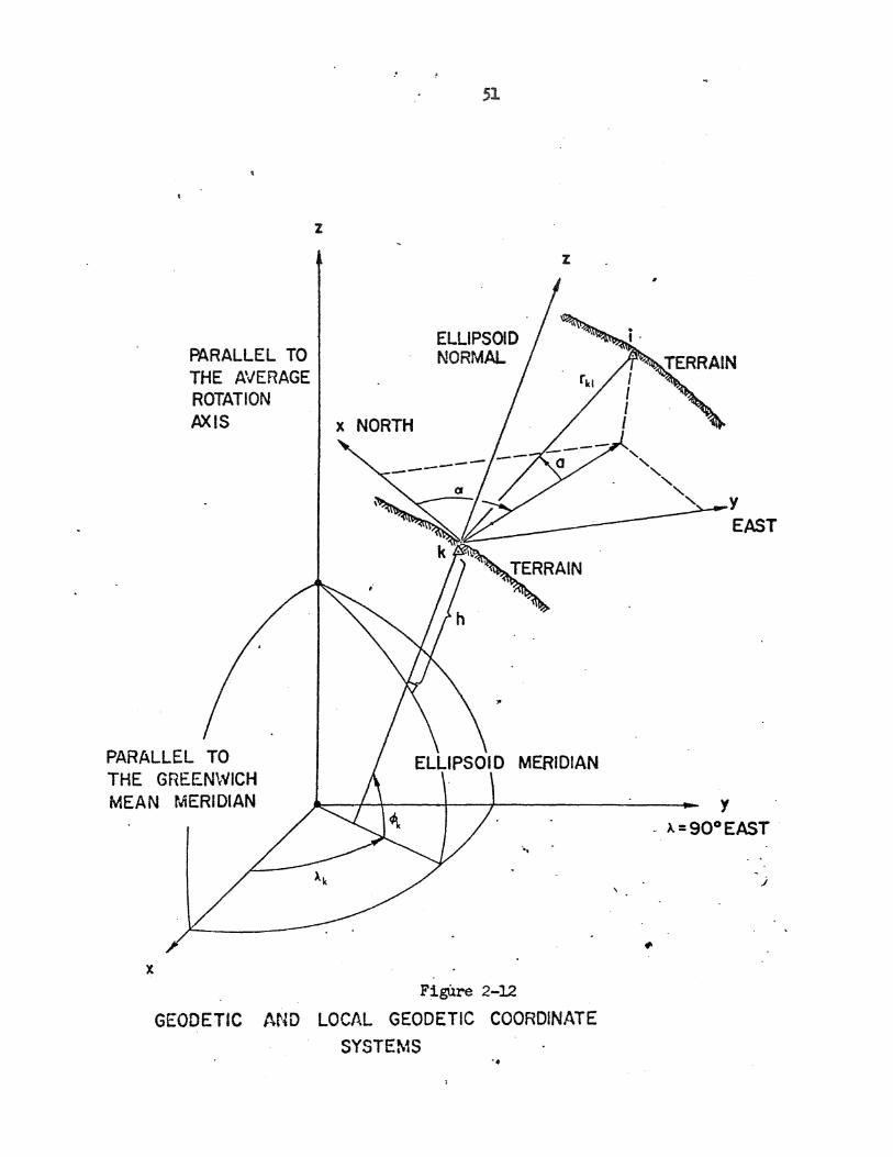
A local geodetic (L.G.) system is specified (see Figure 2-12):
a) The origin lies along the ellipsoidal normal passing
through the observation station. Note that in principle the origin may
lie anywhere along the ellipsoidal normal. In practice it is chosen to
be at the observation station~ at the ellipsoid, or at the intersection
of the ellipsoidal normal with the geoid.
b) The primary pole (z-axis) is the elli-psoidal normal. The
primar:; plane is the plane containing the origin and perpendicular to
the primary pole.
c) The primary axis (x-axis) is the intersection of the
primary plane and the plane containing the semi-minor axis of the
ellipsoid and the origin, and is called t~e.geodetic north.
d) The y-axis is directed east to form a left-handed system.

55
Trar1sformations between local geodetic and local astronomic
systems sharing a common origin can be expressed in terms of the angle
between the ellipsoid normal and gravity vertical (the deflection of the
vertical) and the angle between the geodetic north and astronomic north.
Given the meridian and prime vertical deflection components ~. n respectively,
and the geodetic and astronomic azimuths a, A to a particular point, then
a vector in the local astronomic system is transformed into a vector in the
local geodetic system by
2.65
Note that the order in which the rotations are performed in this case is
not important, since the ~ngles r,, n (A- a) are sma~l enough that their
rotation matrices can be assumed to commute. Note also that if the Laplace
condition is enforced at the origin of these local systems, we have
A- a= (A- A) sin$ = n tan$
If the origin is not at the observation station, the position vector
Rk in 2-61 would refer to the origin, not the observation station. That
is, for a point on the geoid, the computation of (~, yk, zk) is made
from (¢k' Ak' Nk) (geoid undulation), while on the ellipsoid ($k' \k, 0)
are used. Note that when a small region of the earth is taken as a
plane it is a local geodetic system that is implied.
Similar to equations 2-54 and 2-55 the position vector from
observing station k to observed station 1 is given by
X cos ~1 cosakl
<r: k1) T ,., = y = rkl L.u.
cos ~1 sinakl 2-66 z
sin L.G. ~1
and

56
X
z G
X
y
z L.G.
2-67
where (a~ a~ r) are the geodetic altitude, azimuth and range, and
(~, A.} are the geodetic latitude and longitude. Note that the geodetic
system (G) and the average terrestrial system (A.T.) are related by
equation 2-4
X
y = z A.T.
X 0
z 0
+
X
y
z G
where (x , y , z ) are the translation 0 0 0
components of the origin of
the geodetic system in the average terrestrial system.
The unit vectors corresponding to the three Cartesian axes in the
local geodetic system are
,_ -sin4l -COSA
" u. = -sin4l sinA , X --
2-68a
cos4l I. -
--sinA.
" u = COSA ~ y 2-68b
0 I.
,.. -cos4l COSA
A.
cos4l sinA. u = • z 2-68c
sin4> -

57
2. 5 SUMMARY OF TERRESTRIAL SYSTEMS
In this chapter we have precisely defined five specific terrestrial
coordinate systems:
a) Average Terrestrial .(A.T.),
b) Instantaneous Terrestrial (I.T.),
c) Geodetic (G),
d) Local Astronomic (L.A.),
e) Local Geodetic (L.G.),
of which the first three are geocentric and the last two topocentric.
Table 2-4 summarizes the planes, poles and axes defining these systems.
We have also precisely defined four kinds of coordir .. ates:
a) Cartesian (x, y, z) - used by all systems,
b) Curvilinear (', !., h) - used by Geodetic system,
c) Curvilinear (v, A, r) - used by Local Astronomic system,
d) Curvilinear (a, a, r) - used by Local Geodetic system.
Finally we have defined the principal transformations between these
coordinates and coordinate systems. Figure 2-13 lists the equation
numbers which define these transformations, which are tabulated in
Table 2-5.

System
Average Terrestrial
Instantaneous Terrestrial
Geodetic
Local Astronomic
Local Geodetic
Table 2-4.
REFERENCE POLES, PLANES AND AXES DEFINING TERRESTRIAL COORDINATE SYSTE~lli
Reference Poles i Reference Planes Primary· ( z-axis)
: Secondary Primary I Secondary i (x-axis) (1 to Primary Pole)
Handedness
I Average Terrestriali
Pole (CIO)
Instantaneous Terrestrial
Pole
Semi-minor axis (parallel to terrestrial pole)
Gravity Vertical at Station
Ellipsoidal Normal at Station.
H
~ Cb 11 Cll Cb n C1 1-'• 0 ::I 0 111
1-0 11
~ -~
[
I I i
ltAverage Terrestrial equator containing
1 centre of gravity.
Instantaneous Terrestrial
equator.
, Parallel To ! Average Terrestrial i equator
Greenwich mean meridian
Greenwich mean meridian
right
right
right
Cll (I) n 0
g -~--r--==+--Parallel to Greenwich mean
meridian
Astronomic Meridian
of station.
left
I I
Local Horizon ;:g § Cll
Tangent Plane Coincident with I left Geodetic Meridian
of station.
V1 co

Geodetic (G)
Curvilinear («jj,A,h~
Cartesian
Geocentric
Average Terrestrial
(A.T.)
Cartesian
TERRESTRIAL
Instantaneous Terrestrial
(I.T.)
Cartesian
Figure 2-13.
1 Tol>ocentric
Local Astronomic (L.A.)
Local Geodetic · (L.G.)
Cartesian Curvilinear (v,A,r)
Cartesian
EQUATIONS RELATING TERRESTRIAL SYSTEMS
Curvilinear (a,a,r) V1
\0

.·. .,. .... . . ·•.. . ·. ·• ~ . . .... ' . . •.•... ,. ... .. t.,:.·
':'a'cle 2-5.
TRANSFORMATIONS AMONG TERRESTRIAL COORDINATE SYSTEMS.
Original System
Average Instantaneous Geodetic Local Terrestrial Terrestrial Astronomic
··• ...
' Average
[:JAS. + [::]
T errestrial R2(-xp)R1(-yp)
! R (1809.-A)R (90~~)P i
3 2 2
..
Instantaneoun
r:L.T. via I via
Terrestrial R1 (yp R2(xp) Average Average Terrestrial Terrestrial
"'.l
-[~:] r:L I f-'• via via :::1 il' Geodetic Average Local !-'
r:n Terrestrial Geodetic ~ (/1
-+ ~
Local .via via
r:L.A. Astronomic P2R2 (~-90°)R3 (A-180°) Average Local
Terrestrial Geodetic
Local via via Geodetic Geodetic Average P2R2~~-90°)R3(~-180) Ri (-n )R2 t~)
Terrestrial ·-·
Note: ~, A have been corrected fnr polar motion. .:,;.. ...., .... . ..,., v ..... ,.,., '-...
Local Geodetic
via Geodetic
.
via Geodetic
R3 (~80°-A)R2 (90°-~)P2
R2 (+~) R1 (+n)
r:L.G. ..
../
'
'
0'\ 0
...,.

61
3. CELESTIAL COOP~INATE SYSTEMS
Celestial coordinate systems are used to define the coordinates
of celestial bodies such as stars. The distance from the earth to ~
the nearest star is more than 10~ earth radii, therefore, the
~imensions of the earth (indeed of the solar syste12) are almost
negligible compared to the distances to the stars. A second
consequence of these great distances is that, although the stars
themselves are believed to be moving at velocities near the velocity
of light, to an observer on the earth this motion is perceiv~d to be
very small, very rarely exceeding one arcsecond per year. Therefore~
the relationship between the earth and stars can be closely approx-
imated by considering the stars all to be equidistant from the earth,
on the surface of the celestial sphere, the dimension of which is so
large that the earth (and indeed the solar system) can be considered
as a dimensionless point at the centre. Although this point may be
dimensionless, relationships between directions on the earth and in
the solar system can be extended to the celestial aphere.
The earth's rotation axis is extended outward to intersect the
celestial sphere at the north celestial pole (NCP) and south celestial
pole (SCP). The earth's equatorial plane extended outward intersects

62
the celestial sphere at the celestial eguator. The gravity vertical
at a station on the earth is extended upwards to intersect the celestial
sphere at the zenith (Z), and downwards to intersect at the nadir (N).
The plane of the earth's orbit around the sun {the ecliptic plane) is
extended outward to intersect the celestial sphere at the ecliptic.
The line of intersection between the earth's equatorial plane and the
ecliptic plane is extended outwards to intersect the celestial sphere
at the vernal equinox or first point of Aries, and the autumnal
equinox. The vernal equinox is denoted by the symbol ~, and is the
point at which the sun crosses the celestial equator from south to
north.
There are two fundamental differences between celestial systems
and terrestrial or orbital systems. First, only directions and not
distances are considered in celestial coordinate systems. In effect
this means that the celestial sphere can be considered the unit
sphere, and all vectors dealt with are unit vectors. The second
difference is related to the first, in that the celestial geometry is
spherical rather than ellipsoidal as in terrestrial and orbital
systems, which simplifies the mathematical relationships involved.
As discussed in the introduction, there are four main celestial
coordinate systems, called the ecliptic, right ascension, hour angle,
and horizon. Sometimes the right ascension and hour angle systems are
referred to collectively as equatorial systems. We will begin this
chapter by discussing each of these systems in turn.
We noted above that the celestial sphere is only an approximation
of the true relationship between the stars and an observer on the earth.

63
Therefore, like all approximations, there are a number of corrections
which must be made to precisely represent the true relationship. These
corrections represent the facts that the stars are not stationary
points on the celestial sphere but are really moving (proper motion);
the earth's rotation axis is not stationary with·respect to the stars
(precession and nutation); the earth is displaced ~rom the centre of
the celestial sphere, which is at the sun (parallax); the earth is in
motion around the centre of the celestial sphere (aberration); and
directions measured through the earth's atmosphere are bent by refraction.
All these effects will be discussed in section 3.5 in terms of variations
in the right ascension system.
3.1 THE ECLIPTIC SYSTEM
The ecliptic (E) system is specified as follows (see Figure 3-1}!
a) The origin is heliocentric (at the centre of the sun).
b) The primary plane is the ecliptic plane (the plane of
the earth's orbit) and the primary pole (z-axis) is the north ecliptic
pole (NEP).
c) The primary axis (x-axis) is the vernal equinox.
d) The y-axis is chosen to make the system right-handed.
The ecliptic system is the celestial system which is closest to
being inertial, that is motionless with respect to the stars. However,
due to the effect of the planets on the sun-earth~ystem, the ecliptic
plane is slowly rotating (at 0~5 per year) about a slowly moving axis
of rotation.

ECLIPTIC MERIDIAN PLANE OF
C(.)
64
NCP
NEP STAR
Figure 3-l. ECLIPTIC SYSTEM
[x] [en • c.s ~J y & C..···~ z ...
E
ECLIPTIC IIERtOtMI
y

65
The ecliptic meridian is the great circle which contains the
ecliptic poles and the celestial body in question while the ecliptic
meridian of 1r contains the vernal equinox. Ecliptic latitude B is
the angle from the ecliptic and in the ecliptic meridian to the line
connecting the origin to the body. Ecliptic longitude A is the angle
of the ecliptic meridian of the body measured eastwards in the ecliptic
plane from the vernal equinox. The unit vector to a celestial Qody in
the celestial system is
X cosB cosA
y = cosB sin>..
sinS
and the angles are related to the Cartesian components by
. -1 B = Sl.n z '
3.2 THE RIGHT ASCENSION SYSTEM
3-1
3-2
3-3
The right ascension (RA) system is specified as follows (see
Figure 3-2).
a) The origin is heliocentric~
b) The primary plane is the equatorial plane, and the
primary pole (z-axis) the north celestial pole (NCP).
c) The primary axis (x-axis) is the vernal equinox.
d) The y-axis is chosen to make the system right-handed.
The right ascension system is the most important celestial system. It

EQUINOCTIAL COLURE PLANE
X
Figure 3-2.
66
•
NCP ...........
tc .. a c. •]· ... CH 8 ltft e. ... :
.__CEL&STtM. STM81011Y
CELESTIAL EWIITOftiAL PLAt~£
RIGHT ASCENSION SYSTE·M

67
is in this system that star and satellite coordinates are published,
and-it serves as the connection between terrestrial,celestial and
orbital systems.
The secondary plane contains the north celestial pole and the
vernal equinox and is called the eguinoctialcolure plane. The hour
circle is the great circle_containing the celestial poles and the
body in question. The declination o of a body is then the angle
between the celestial equator and a line joining the origin to the
body. The right ascension a is the angle measured in the equatorial
plane eastwards from the vernal equinox to the hour circle passing
through the body in question. The unit vector describing the direction
of a body in the right-ascension system is
X coso cosa
y = coso sina • 3-4
z R.A. sino
The right ascension system is related to the ecliptic system
by the acute angle between the ecliptic and celestial equator,
called the obliquity of the ecliptic, and denoted~. Therefore
X X
y = y 3-5
z R.A. z E
3.3 THE HOUR ANGLE SYSTEM
The hour angle (HA) system is specified as follows (see Figure 3-3):
a) The origin is heliocentric.
b) The primary plane is the equatorial plane.

CELESTIAL MERIDIAN __ -"" PLANE
X
68
Figure 3-3. HOUR ANGLE SYSTEM
STAR

c) The secondary plane is the celestial meridian plane of
the observer. The primary axis (x-axis) is the intersection between
the equatorial and observer's celestial meridian planes.
d) The y-axis is chosen so that the system is left-handed.
The hour angle system rotates with the observer.
·T~e hour angle h is the angle measured westward in the equatorial
plane from the observer's celestial meridian to th~ hour circle of
the body in question. The angle measured up from the equatorial plane
to the line directed from the origin towards the body is the declin
ation o.
The unit vector describing the direction of a celestial body in
the hour angle system is
X
·y
z H.A.
=
cos 0 cos h
cos o sin h •
sin o
3-6
We have so far defined four meridians on the celestial sphere:
that containing the vernal equinox (the equinoctial colure); the
Greenwich meridian; that containing the observer (the celestial
meridian); and that containing the star (the hour circle). Figure 3-4
shows the relationships between these meridians.
From the vernal equinox counterclockwise to
a) the Greenwich meridian is called Greenwich Sidereal
Time (GST),
b) the celestial meridian is called l-ocal Sidereal Time
(LST),
c) the hour circle is called the right ascension (a).

X-AXIS OF RIGHT ASCENStON
SYSTEM
7n i"""
CELESTIAL EQUATOf't
NCP
TOP VIE:W
OF CEl.ESTIAL
SPMI:.W:
GREENWICH MERtOIAH
HOUR CtRCLE T~STAft
X-AXtS OF 110Uft AMGLE
STSTft
X-AXIS OF TERRESTRIAL
~YS'f'£'M
·-~ ....... ___ ...... __
Figure 3-4.
TIME, LONGITUDE, AND RteHT ASOENS"'"

71
From the Greenwich meridian counterclockwise to the celestial meridian
is called the astronomic longitude {A). From the celestial meridian
clockwise to the hour circle is called the hour angle (h). Therefore,
and
LST = GST + A
LST = h + a
h = GST + A - a
3-7
3-8
3-9
The hour angle system is related to the right ascension system
by the local sidereal time (LST). That is
X X
y y 3-10
z HA
3.4 THE HORIZON SYSTEM
The horizon (H) system is specified as follows {see Figure 3-5).
a) The origin is heliocentric.
b) The primary pole (z-axis) is the observer's zenith
(gravity vertical}. The primary plane is the observer's horizon.
c) The primary axis (x-axis) is the north point.
d) The y-axis is chosen so that the system is left-handed.
The horizon system is used to describe the position of a
celestial body in a system peculiar to a topocentrically located
observer, similar to the local astronomic system described in the
chapter on terres~rial systems. The main difference is that the
origin of the horizon system is heliocentric instead of topocentric.

ZENITH
\ '
SOUTH
CELESTIAL HORIZON
Pl.ANE
Figure 3-5.
HORIZON SYSTEM
NORTH
y

73
The great circle containing the primary pole and the celestial
body being observed is called the vertical circle. The location of
this great circle is given by the astronomic azimuth A, the angle
measured clockwise in the horizon plane from north to the vertical
circle. The altitude a of the body is the angle between the horizon
plane and the line directed .from the origin of the system toward the
body. The unit vector to a celestial body in the horizon system is
X cos a cos A
y = cos a sin A 3-11
z sin a
The horizon system is related to the hour angle system by the
astronomic latitude ~. That is
X X
y y 3-12
z H z HA
3.5 VARIATIONS OF THE RIGHT ASCENSION SYSTEM
As mentioned at the beginning of this chapter, the celestial
sphere approximation requires corrections for precise work. These
corrections are for proper motion, precession, nutation, aberration,
parallax and refraction, and are applied in four stages between the
system in which observations are actually made (which we will call
the "observed place system at epoch T") and the most absolute right
ascension system (which we will call the "mean celestial system at
standard epoch T "). We will consider these systems in the reverse 0
order, that is:

74
a) mean celestial system at standard epoch T0 ,
b) mean celestial system at epoch T,
c) true celestial system at epoch T,
d) apparent place system at eppch.T,
e) observed place system at epoch T.
The connections between these five systems are shown in Figure 3-6.
The first three systems are related by motions of the coordinate
system, while the last two are related by physical effects which
cause the position of the celestial body to vary.
3.5.1 Precession and Nutation
The earth is not perfectly spherical, but has an equatorial bulge
which is attracted by the sun, moon, and planets in a non-~etrical
way. This causes the earth's axis of rotation (th~ north celestial
pole) to move around the north ecliptic pole with a period of about
25,800 years and an amplitude equal to the obliquity of the ecliptic
(23~5). This motion is called precession and is similar to the
precession of an ordinary gyroscopic top about the gravity vector
[Mueller 1969, pages 59-62].
Precession is itself not a regular motion sin~e the earth's
orbit is not circular and the moon's orbit does not lie in the ecliptic
plane, and is not circular. Therefore, the added effects of the sun
and moon are constantly changing as their configuration changes.
Irregularities in precession are called nutation, and for the celestial
pole have a period of about 18.6 years and a maximum amplitude of
about 9". The added irregularity due to the chang) ng configuration of

1.1
Mean @ T 0
Proper Motion Precession
Nutation
Annual Aberation Annual Parallax
Diurnal Aberation Geocentric Parallax
Refraction
Observed @ T
Figure 3-6.
VARIATIONS OF THE CELESTIAL RIGHT ASCENSION SYSTEM

76
the planets is called planetary precession, and causes the very slow
motion of the ecliptic plane mentioned in section 3.1. In principle,
precession exists only because the earth has an equatorial bulge, and
nutation and planetary precession exist only because precession
exists.
Precession and nutation are shown schematically in Figure 3-7.
The celestial equator is defined as being perpendicular to the
celestial pole, so that it too follows the precession and nutation of
the pole. The vernal equinox is defined as being at the intersection
of the celestial equator and ecliptic, so that it ~ill follow both
the precession and nutation of the celestial equator, and the motion
of the ecliptic due to planetary precession. The effects are shown
in Figure 3-8.
3.5.2 Mean Celestial Systems
A mean celestial (M.C.) system is specified as follows.
a) The origin is at the centre of the sun.
b) The primary pole (z-axis) is a precessing (but not
nutating) pole which follows the precession of the north celestial
pole, and is called the mean celestial pole.
c) The primary axis (x-axis) is a prece!:sing (but not
nutating) axis which follows the motion of the vernal equinox due both
to precession of the celestial equator and rotation of the ecliptic,
and is called the mean vernal eguinox.
d) The y-axis is chosen so the system is right-handed.

ECLIPTIC POLE
GENERAL PRECESSION
PATH OF MEAN CELESTIAL POLE
77
~TH OF TRUE CELESTtAL 'POLE
P=PftECESStON
NT :: NUT.ION ~T
Fig,ure :-1. MOTION OF CELESTIAL POLE

Gfc>
ECLIPTIC AXIS TRUE CELESTIAL AXIS
TRUE CELESTIAL AXIS
(EXTENSION OF ROTAT tON AXtS OF EARTH ) .
TRUE EQUATOR OF EARTH AT T1 •
.. :::::::_-1\ INTERSECTION OF ("\ ECLIPTIC WITH EARTH.
/ ECLIPTIC PLANE TRUE EQUATOR OF EARTH AT
T0 ( PLAME 1 TRUE C!LESTtAL AXtS).
Figure 3-8. ·THE EFFECT OF PRfCI!S9tON M«> NUT AltON
-·~ 0:.)

79
Because the mean celestial system is moving, the coordinates
(right ascension a, and declination 6) of celestial bodies vary with
time. Therefore, for each epoch of time~' a different mean celestial
system is defined. Certain epochs T0 have been chosen as standard
epochs, to which tabulated mean celestial coordinates of celestial
bodies refer. The relationship between mean celestial systems of times·
T0 and T is usually defined in terms of the precessional elements
(' , e, z) as shown in Figure 3-9. Expressions for these elements as 0
a function of time were derived over 70 years ago by Simon Newcomb
[Mueller 1969, p. 63]. The angles (90°-t ) and (90°+z) are the right 0
ascensions of the ascending node of the equator at T measured
respectively in the systems at T and at T. The angle e is the 0
inclination of the equator at T with respect to the equator at T • 0
The transformation from a mean celestial system at T to one·at Tis 0
given by
X X
y y 3-13
z M.C.T. z _ M.C.T0
Independent of the motion of the mean celestial coordinate
system due to precession, each star is changing in position due
to proper motion. Because this proper motion is uniform, it is
most appropriate to account for it in the most uniform right
ascension system, that is the mean celestial system. The proper
motion components for each star of interest (usuall~· tabulated

NCP(T0 )
80
NCP(T)
~(T)
PftECESSION
Gl.· .. . MC.To
Figure· 3-9. MEAN CELESTIAL COOftOINATE SYST£MS
MI•N EOtJaTOR . ·····'t)\• ..

81
as rates of changes in right ascension and declination) must therefore
be included in the conversion of mean place at T to mean place at T. o·
3.5.3 The True Celestial System
A true celestial system (T.C.) is specified as follows.
a) The origin is at the centre of the sun.
b) The primary pole (z-axis) is a precessing and nutating
pole which follows the precession and nutation of the north celestial
pole, and is called the true celestial pole.
c) The primary axis (x-axis) is a precessing and nutating
axis which follows the motion of the vernal equinox due to precession
and nutation of the celestial equator, arid to rotation of the ecliptic,
and is called the true vernal eguinox.
d) The y-axis is chosen so the system is right-handed.
As in the case of mean celestial systems, a different true
celestial system is defined for each epoch of time T. The true
celestial sy"stem at epoch T differs from the mean celestial system
at epoch T only by the effect of nutation, and the relationship is
usually defined in terms of the nutation in longitude 8~ and
nutation in obliquity f:l.e. shown in Figure 3-10. Expressions for these
two elements as a function of time, and other parameters were derived
by Woolard [~~eller 1969, p. 69]. The transformation from a mean
celestial system at T to a true celestial system at T is given by
r- -X
y
z ._ - T.C.T.
:- -X
·z __ M.C.T •
3-14

O'fO (TRUE)
NCP(MEAN);; NCP (TRUE)
t«-'
NUTATION
82
. TRUE EOUATOMAL
PLANE AT T
TRUE AND MEAN CELESTIAL COORDINATE SYSTEMS. Fi~~~-3=1o~ ..

83
3.5.4 The Apparent Place System
An apparent place (A.P.) system is specified as follows.
a) The origin is at the centre of the earth.
b) The primary pole is parallel to the true celestial pole.
c) The primary axis is parallel to the true vernal equinox.
d) The system is right-handed.
Therefore, an apparent place system is a true celestial system with
the origin shifted from the centre of the sun to the centre of the
earth. This means the origin is no longer at the centre of the true
celestial sphere which causes annual parallax, and the origin is
revolving around the centre of the true celestial sphere which causes
annual aberration.
If the. earth's orbit is regarded as circular, the earth has a
constant of aberration.
v K = c
n cosec 1" = 20.4958 3-15
where v is the earth's velocity and c the velocity of light; and the
radius of the earth's orbit will subtend a different angle H at each
star, called the stellar parallax for that star. The nearest star
has a stellar parallax of 0':16.
The right ascension a and declination o of a star expressed in
the apparent place system is then [Mueller 1969, pages 93 and 61].
+ 3-16
where

Ah
cos£ seco - sina cosA 5 seco = n [ ::p] [coso }-17
coso sin£ sinA 5 - cosa sino cos).. 5 - sina sino COSE sinAS p
and
[AoA1 [coso casAs cos£ seco + sina sinAs secO J = -K 3-18
MA COS As cos£(tanc coso - sina sino) + ccsa sino sinAs
and As is the longitude of the sun, £ the obliquity of the ecliptic,
and (a, o) in 3-17 and 3-18 expressed in the true celestial system.
The fact that the earth's orbit is not circular introduces
errors of about 1% in equation 3-17 and up to 0'!343 in equation 3-18.
3.5.5 The Observed Place System
An observed place (O.P.) system is specified as follows.
a) The origin is at the observing station.
b) The primary pole is parallel to the true celestial pole.
c) The primary axis is parallel to the true vernal equinox.
d) The system is right-handed.
Therefore, an observed place system is an apparent place system
with the origin shifted from the centre of the earth to the observing
station. This means the origin is no longer at the centre of the
earth, which causes geocentric parallax, and the·origin is rotating
around the centre of the earth, which causes diurnal aberration. In
fact, the effect of geocentric parallax is always negligible when
observing stars. The diurnal constant of aberration is
v k = c
cosec 1" = O'! 320 p coscp 3-19

~here v is the earth's surface rotational velocity, c is the velocity
of light, p is the radial distance from geocenter to observer in units
.. of earth radius, and~ is the geodetic latitude of the observer.
There is a third effect due to the fact that the earth is
blanketed with an atmosphere of varyi,ng optical density. This
·~auses a complex change in the direction of the light ray from a star
which depends on the incident angle. Mueller [1969, pages 103-109]
discusses this atmospheric refraction in detail.
The right ascension and declination of a star in the observed
place system is then
3-20
where
k [cos h
sinh
seco J sino
3-21
where h is the hour angle of the star, and (6aR, 6oR} are the
corrections due to refraction.
3.6 TRANSFORHATION BETWEEN APPARENT CELESTIAL AND AVERAGE
TERRESTRIAL COORDINATE SYSTEHS
The apparent celestial and average terrestrial coordinate systems
both have
a) their origins at the centre of gravity of the earth,
b) their primary poles as the era pole, that is the
average terrestrial pole is parallel to the true celestial pole,
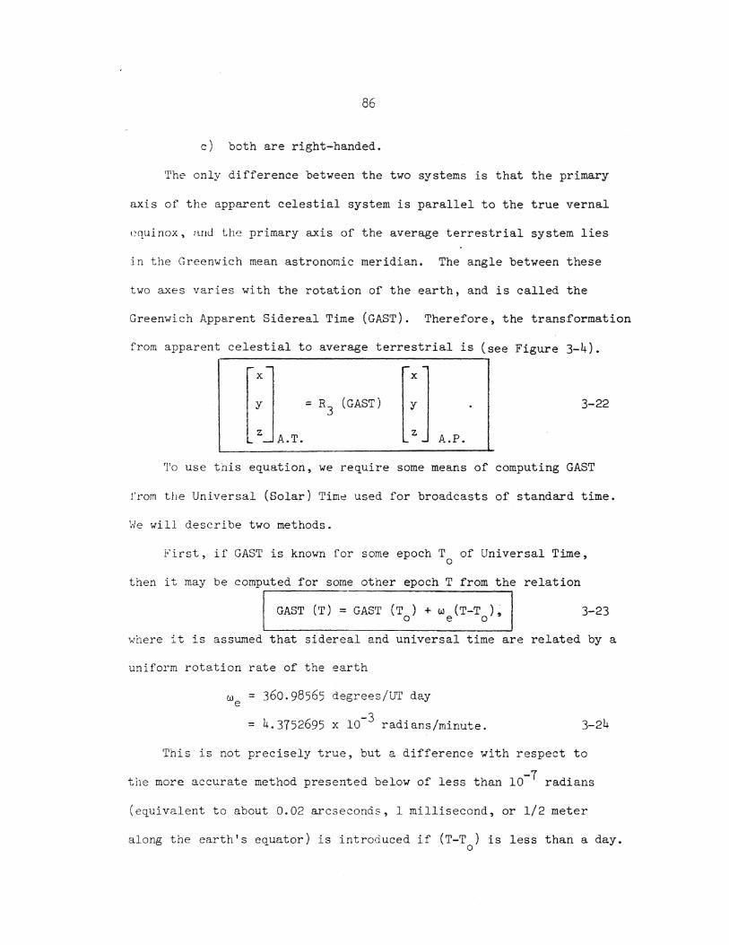
86
c) both are right-handed.
'l'he only difference between the two systems is that the primary
axis of the apparent celestial system is parallel to the true vernal
equinox, ami the primary axis of the average terrestrial system lies
in the Greenwich mean astronomic meridian. The angle between these
two axes varies with the rotation of the earth, and is called the
Greenwich Apparent Sidereal Time (GAST). Therefore, the transformation
from apparent celestial to average terrestrial is (see Figure 3-4).
X X
y = R3 (GAST) y 3-22
z A.T. z A.P.
'l'o use this equation, we require some means of computing GAST
from the Universal (Solar) Time used for broadcasts of standard time.
'.-le will describe two methods.
First, if GAST is known for some epoch T of Universal Time, 0
then it may be computed for some other epoch T from the relation
GAST (T) = GAST (T ) + w (T-T )~ o e o 3-23
where it is assumed that sidereal and universal time are related by a
uniform rotation rate of the earth
we = 360.98565 degrees/UT day
= 4.3752695 x 10⁻³ radians/minute. 3-24
This is not precisely true, but a difference with respect to
ti1e more accurate method presented below of less than 10-7 radians
(equivalent to about 0.02 arcseconds, 1 millisecond, or 1/2 meter
along the earth's equator) is introduced if (T-T ) is less than a day. 0

1-\ more a<:curate :relation is given by Veis [1966, p. 19}:
r--· I JAS1' =
I 1!~392 X 10-3 sin (12'?1128 - 0'?052954 T)
+ 0'?053 X 10-3 sin 2 ( 12'?1128 - 0'?052954 T) 3-25
0'?325 X l0-3 sin 2(280~0812 + 0'?9256473 T)
:.'~1ere T is the number of Julian Days since the epoc~ CL 5 January 1950
(that 1s midnight of December ~1, 1949). For 1971
T = 7669 + D + (~ + S/60)/1440 3-26
the Ja:v number during 1971,
= the minute of UT time,
S = the second of UT time,
·md 7669 is the nu1nber of days beb,-een January 1, 1950 and December 31,
'970. This expression is accurate to 0.2 arcseconds, 10 milliseconds,
•Jr 5 !rleters along the equator for any value (T - T0 ). r·1ore accuracy
c:an be obtained by adding more terms (:-Jautical Almanac Office 1961].
3. '( SUN!·JI..F:Y C.F C:::LESTIAL SYST2·~S
r~ this chapter we have d~fi~ed four celestial coordinate systems:
a) Ecliptic (E),
b) Rig~t Ascension (5.A. ),
c) Hour Angle (H.A.),
d) Horizon (H.).
~able 3-l SlW~arizes the reference poles, planes and axes defining
the s:.rstems. 'l'ab2_e 3-2 SUElffiari=es ·~he transformations between these

88
systems.
\~P hav.:• a1~~n precisely d0t'i.ned four variations to the right
a:.~c!c:'Tl!~ iun Bystem;
a) ~lean Celestial (i.L C. ) ,
b) 'i'ruc~ t~elesti aJ ('J' .C.),
c) Apparent Place (A.P.),
d) Observed Place (O.P.),
all of which vary with time, so that the epoch T to which they refer
must be specified. Figure 3-ll shows the parameters which connect all
of these celestial coordinate systems.
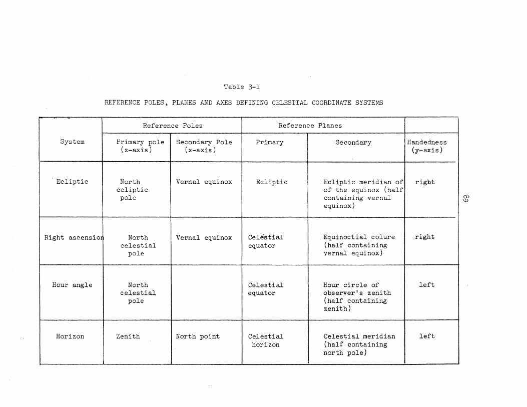
'l'able 3-1
REFERENCE POLES, PLANES AND AXES DEFINING CELESTIAL COORDINATE SYSTEMS
-Reference Poles Reference Planes
System Primary pole Secondary Pole Primary Secondary (z-axis) (x-axis)
Ecliptic North Vernal eq_uinox Ecliptic Ecliptic meridian of ecliptic. of the eq_uinox (half pole containing vernal
eq_uinox)
Right ascensio North Vernal eq_uinox Celestial Eq_uinoctial colure celestial eq_uator (half containing
pole vernal equinox)
Hour angle North Celestial Hour Circle of celestial eq_uator observer's zenith
pole (half conta:ining zenith)
Horizon Zenith North point Celestial Celestial meridian horizon (half containing
north pole)
r--------1 -j
Handedness !
(y-axis)
right
I
right
left
left
co \0

Ecliptic
'">j .... Right ::s
I» Ascension 1-'
en « (ll
ct (1)
s Hour
Angle
Horizon
Table 3-2
TRANSFORMATIONS ANONG CELESTIAL COORDINATE SYSTEMS.
Original System
Ecliptic Right Ascension Hour Angle
r:t Rl (£)
'
Rl (-£)
[:] R.A.
R3 (-LST) P 2
P 2 R3(tLST) [:L.A. R3(180°) R2 (90°-~)
Horizon
R2 (~-90°) R3(180°)
r:L.
'
\D 0

Ecliptic
Mean Celestial @ T
0
Figure 3-11. Celestial Coordinate Systems.
Right Ascension
Mean Celestial @ T
Hour Angle
True Celestial @ T
Horizon
Apparent @ T
Observed @ T
1.0 1-'

92
4. THE ORBITAL COORDINATE SYSTn4
In this chapter we discuss the orbital system, which is used to
define the coordinates of a satellite orbiting around the earth. We
first discuss the orbital ellipse, and the coordinate system in the
orbit plane. Then we transform this system into the apparent celestial
and average terrestrial systems, and discuss variations in the orbital
elements. Finally expressions for the coordinates of the satellite
subpoint,and the topocentric coordinates of the satellite are derived.
4.1 THE ORBITAL ELLIPSE AJID ORBITAL ANOMALIES
The trajectory of a body moving in a central force field describes
an ellipse, with the attracting force centred at one of the foci of the
ellipse.
In the case of a satellite orbiting around the earth, this is
called the orbital ellipse, and the centre of gravity of the earth is
at one of the foci (see Figure 4-1). The point of closest approach of
the satellite to the earth is called the perigee, and the farthest
point is called the apogee. Both perigee and apogee lie on the semi-
major axis of the ellipse, called the line of apsides. The size and
shape of the orbital ellipse are usually defined using the semi-major
axis, a and the eccentricity e, where
2 e = 3-1
and b is the semi-minor axis of the ellipse.

93
y
f~ TftUE MIOMALY a
E- ECGdl'fMt AW-ALY
APOGEE X
-· ae PStllt
l EARTH (focus)
) · 6EOME;fRI C CENTRE ....
a
FIGURE 4-l ORBIT ELLIPSE

94
Consider the satellite to be at a point m on the orbital ellipse.
The angular distance between perigee and m is called the satellite
anomaly. There are three anomalies. The true anomaly f is the angle
between the line of apsides and the line joining the focus to the
satellite.
Consider the projection of the satellite position m along a line
parallel to the semi-minor axis to intersect a circle with radius
equal to the semi-major axis at a point m'. The eccentrLc anomaly E
is the angle between the line of apsides and the line joining the
geometric centre of the ellipse tom'.
The mean anomaly M is the true anomaly corresponding to the motion
of an imaginary satellite of uniform angular velocity, that is M = 0
at the perigee and then increases uniformly at a rate of 360° per
revolution. When this is expressed as a rate per unit time, then it is called the mean anomalistic motion n.
The relationship between the true anomaly f and the eccentric
anomaly E is from Figure 4-1
[J = cos E - ae] = [a(cos
a(l -4-2
sin E sin
or
tan f cos E - e 4-3
The relationship between the eccentric anomaly E and the mean
anomaly M is Kepler's e~uation [Kaula 1966, p. 23]
M = E - e sin E. 4-4
where M and E are in radians.

95
We are usually given the mean anomaly M, and want to find the
eceentrlc anomaly E from equation 4-4. We will present three ways.
If the eccentricity is very small (say e ~ 0.002), then thee sinE
term will be small, and M ~ E. Therefore we can write
I E = M + e sin E = M + e sin M ·I 4-5
For an eccentricity of e = 0.002 this approximation introduces an error
-6 of about 10 radians.
If greater precision is required or the eccentricity is not so
small, we can solve 4-4 iteratively. Taking the total differential of
4-4
or
6!-1 = ( l - e cos E) 6E
oM 6E = --'-----1 - e cos E 4-6
Given M, the iterative solution of 4-4 begins by making an initial
approximation from 4-5 as
E0 = r.1 + e sin M
The following equations are then iteratively evaluated in order
M. = E.- e sin E. 1 1 1
t1M = M. H
tlE =
1
l - e cos E. 1
until the difference frM is less than some chosen £.

96
A third method of evaluating E is to use a power series in e, for
example [Brouwer and Clemence 1961, p. 76]:
1 3 1 5 1 7 E = l'-1 + (e - 8 e + 192 e - 9216 e ) sin M +
1 2 1 4 1 6 + <2 e - 6 e + 98 e ) sin 2M +
27 5 243 7 128 e + 5120 e ) sin 3M +
1 4 4 6 (125 5 + (3 e - 15 e ) sin 4M + 384 e
+ 27 6 sin ~~ + 16807 e7 Bo e ... Ol'l 46o8o sin 7M
4.2 THE ORBITAL COORDINATE SYSTEM
4-7
The orbital (ORB) coordinate system is specified as follows (see
Figure 4-2) :
a) The origin is at the centre of gravity of the earth.
b) The primary plane is the plane of the orbital ellipse,
and the primary pole (z - axis) is perpendicular to this
plane (see Figure 4-1) .
c) The primary axis (x- axis) is the line of apsides.
d) The y-axis is chosen so that the system is right-handed.
The position vector of the satellite in its orbit is given by
X cos f a (cos E - e)
r = y = r 4-8
z ORB 0 0
Note z = 0 because the satellite is assumed not to be out of the orbit
plane.

GREENWICH
y TRUE VERNAL EQUINOX
9T
FIGURE 4-2 KEPL£ft1Aft ORBITAL ELEMENTS
0 - SEMI MAJOR } SIZE AND SHAPE OF OMIT e- ECCENTRICITY
w- ARGUMENT OF PERIGEE- OfRECTION OF LlN£ Of' APseES} .0. .. -RIG. HT ASCENSION OF lfSCENOING NOD£ Ns!TIGN OF ORBtT i -l.tiQ.tMAT ION
~ f- TRUE :ANOMALY AT TiME T ·

98
4.3 TRANSFORMATION FROM ORBITAL TO AVERAGE TERRESTRIAL SYSTEM
The orbital plane does not rotate with the earth, but· remains fixed
in the celestial system. The orbital system and the apparent celestial
both have their origins at the centre of gravity of the earth.
From Figure 4-2 we see that when the orbital plane is extended to
meet the celestial sphere, it intersects the celestial equator at the
ascending node (where the satellite croses the equator from south to
north), and the descending node. The angle between the celestial
equator and the orbital plane is the inclination i. The angle between
the ascending node and the line of apsides, measured in the orbital
plane is the argument of pergiee w. The angle between the vernal
equinox and the ascending node, measured in the celestial equatorial
plane is the right ascension of the ascending node n.
The transformation from the orbital system to the apparent
celestial system is
X X
y y
z z ORB
4-9
The transformation from apparent celestial to average terrestrial
is given by equation 3-22, so that
X X
y y 4-10
z A.T. z ORB

99
4. 4 VARIATIONS IN THE ORBITAL ELEMENTS
So far we have assumed that the satellite orbit does not vary with
time, and is completely specified by the six Keplerian orbital elements
a, e, f, w, i, n. The earth 1 s gravitational force field is not
spherically symmetric, as evidenced by geoid undulations and the
equatorial bulge. Also the atmosphere exerts a fluctuating drag force
on the satellite. Because of these and other smaller effects, the
satellite trajectory cannot be assumed to be a fixed ellipse. However,
for each epoch of time T there will be a different orbital ellipse
tangent to the satellite trajectory at that epoch. Each of these
different ellipses will have a set of Keplerian orbital elements, and
if the variation in these orbital elements with time is known, they
are said to describe an osculating orbital ellipse which describes the
satellite trajectory accurately.
The variation with time of the inclination angle is equivalent to
introducing a time-varying out-of-plane component, and this is often
done. For nearly circular orbits, the eccentricity is small to start
with, so variations are usually neglected.
4.5 THE SATELLITE SUBPOINT
The subpoint of a satellite is simply the trace of the path of
the satellite on the ellipsoid (see Figure 4-3}. The coordinates of
the subpoint are given by the geodetic latitude ~ and longitude A of
the ellipsoi.dal normal passing through the satellite.
The average terrestrial Cartesian coordinates of the satellite
are Roown from equation 4-10. From equation 2-32

10.0 ..
ROTATIONt--•L AXIS SAT£ lUTE
,
Figure 4-3 SATELLITE SU8POfNT

X
y =
z A.T.
Yo +
Zo
101
(N + h} cos' COSA
(N + h) cos~ sinA
rnb2 /a2 +h) sin'
and if the reference ellipsoid parameters (a, b, x0 , y 0 , z0 ) are known
this equation can be iteratively inverted to solve for (,, A, h) using
the method of section 2.2.6.
4.6 TOPOCENTRIC COORDINATES OF SATELLITE
If we are observing a satellite at position j from a station i
on the earth (see Figure 4-4), then we will require an expression for
the coordinates of the satellite in the local geodetic system of station
i.
If the coordinates (<Pi, A.i_, IJ_) of station i are known with respect
to a reference ellipsoid (a, b, x 0 , y 0 , ~0 ) then the geodetic Cartesian
coordinates of i
x. ~
r. = yi 4-11 ~
z. G ~
can be computed from equation 2-31.
If the average terrestrial Cartesian coordinates of j have been
computed by the methods outlined in this chapter, then the geodetic
coordinates of j are
xj Xo
rj = yj Yo 4-12
z. A.T. Zo J

Figure 4-4
102
LOCAL GEOOETIC SYSTEM
\ \ \ \ I
' I I I I I I
I I
I I
TOPOCEHTPtlC CO()ft{)fNATES (W MTE'LLIT£

103
The range vector from l to j is
lv - xil .... ...,
I ~. I:: I I J ~ = r. r. =iv yi = • .....
lJ J l. v j
L zj - z. l ~zJ " l.J G. \.1
The coordinates of the range vector can be expressed in the local
geodetic system by using equation 2-67
r~x
l~y ~z L.G.
But from equation 2-66
t:,.y r
cos
= 6r cos a sin a
a cos a
fJ.zJ ~ G L. •
lsin a
where the range
and the altitude a and azimuth a are given by
-1 a = sin
a = -<-an - 1 (!&._) " t-,x
4-13
4-14
4-15
4-16
4-17
4-18

104
5 . SUMMARY OF COORDINATE SYSTEMS
In this chapter we will summarize the relationships between the
coordinate systems dealt with in these notes. We will also explain a
duality paradox which has arisen earlier in the notes. This chapter
is, in effect, an explanation of the symbols and abbreviations used in
Figure 5-l.
5.1 TERRESTRIAL SYSTEMS
We discussed five terrestrial systems:
a) I.T. = Instantaneous Terrestrial Coordinate System,
b) A.T. = Average Terrestrial Coordinate System,
c) G. = Geodetic Coordinate System,
d) L.G. = Local Geodetic Coordinate System,
e) L.A. = Local Astronomic Coordinate System,
which are related to each other by the four sets of parameters
a) Polar Motion (xp, yp) -relates I.T. and A.T .. ,
b) Translation of the origin (x0 , y 0 , z 0 ) -relates A,T, and G.,
c) Geodetic Latitude and Longitude(~, X}- relates G. and L.G.,
d) Astronomic Latitude and Longitude (~, A} - relates A.T •.
and L.A.

Figure 5-l
COORDINATE SYSTEMS.
I ~ERRESTRIAL ""§ys~EMS]
Diurnal
HELIOCENTRIC GEOCENTRIC TOPOCEN'rRIC
..... 0
\11

106
5. 2 CELESTIAL SYSTEMS
We discussed four main celestial systems
a) E. = Celestial Ecliptic Coordinate System,
b) R.A. = Celestial Right Ascension Coordinate System,
' c) H.A. = Celestial Hour Angle Coordinate System,
d) H. = Celestial Horizon Coordinate System,
which are related to each other by the three parameters
a) Obliquity of the ecliptic (e:) - relates E. and R.A.,,
b) Local Sidereal Time (LST)- relates R.A. and H.A.,
c) Astronomic Latitude (~} - relates H.A. and H.
The R.A. system has four variations
a} M.C. =Mean Celestial Coordinate System,
b) T.C. = True Celestial Coordinate System,
c) A.P. = Apparent Place Coordinate System,
d) O.P. = Observed Place Coordinate System.
which all vary with time and thus are defined only when the epoch T
to which they refer is specified.
The parameters relating these systems are
a) Precession and Proper Motion - relates M.C. at standard
epoch T and M.C. at epoch T, 0
b) Nutation - relates M.C. and T.C., both at epoch T,
c) Annual Aberration and Parallax - relates T.C. ru1d A.P.
both at epoch T,
d) Diurnal Aberration, Geocentric Parallax and Refraction -
relates A.P. and O.P. at epoch T.

107
5.3 DUALITY PARADOX IN THE APPARENT AND
OBSERVED CELESTIAL SYST~fS
The reason there are apparent and observed systems is because
the observer is not at the centre of the celestial sphere (the centre
of the sun) and this must so~ehow be accounted for. There are two
ways of making this correction, and this difference has not been made
explicit earlier in these notes.
First we can retain the true celestial system (with heliocentric
origin) as our coordinate system, and apply corrections to the positions
of the stars. This is the approach described in sections 3.5.4 and
3.5.5 where the aberration and parallax corrections are applied to the
right ascension and declination, and do not change the coordinate system.
Therefore, we then say that the stars have "apparent places" or
"observed places" in the true celestial system.
The second approach is to actually move the origin of the true
celestial system from the centre of, the sun to the centre of the earth
(for the apparent system) and to the observer's position (for the
observed system}. This is what we have done when we related the average
terrestrial to the celestial system in section 3.6 and the orbital
system to the celestial system in section 4.3. In ~his case we called
the shifted true celestial system the "apparent celestial system". In
other words we have adopted the convention that
a) "true" means heliocentric,
b) "apparent" means either geocentric or corrected :for the
heliocentric-geocentric shift,
c} "observed" means either topocentric or corrected for the
heliocentric-topocentric shift.

108
Two connecting parameters, Proper Motion .. and Refraction, do not
fit in to this second scheme. Proper Motion is the changes in the
positions of stars, and is different for each star. Therefore a
different coordinate system would have to be defined for each star,
which is nonsense. The magnitude of the refraction correction
depends on the incident angle and the ambient conditions. Therefore
specifying that the coordinate system follow refraction would mean a
different coordinate system for each incident angle, all of which would
be jumping around with the temperature and wind.
5 • 4 THE CONNECTIONS BETWEEN TERRESTRIAL,
CELESTIAL AND ORBITAL SYSTEMS
The average terrestrial and apparent celestial systems are connected
by GAST (Greenwich Apparent Sidereal Time). Note that the use of
"apparent" in GAST is consistent with the convention we adopted in the
previous section. That is, "apparent" means "geocentricR.
The orbital and apparent celestial systems are connected by the
Euler angles
a} w = argument of perigee,
b) i = orbital inclination,
c) Q =right ascension of the ascending node,
To summarize the differences between terrestrial, celestial and
orbital systems:
a) terrestrial systems rotate and revolve with the earth,
b) celestial systems do not revolve with the earth,
c) orbital systems do not rotate with the earth.
109
REFERENCES
Bamford, G. (1971). Geodesy, Third Edition, Oxford University Press, London.
Brouwer, D. and G.M. Clemence (1961). Methods of Celestial Mechanics. Academic Press, New York.
Goldstein, H. (1950). Classical Mechanics. Addison-Wesley Publishing Company, Reading, Massachusetts.
Heiskanen, W.A. and H. Moritz (1967). Physical Geodesy. W.H. Freeman and·co., San Francisco.
Kaula, William M. (1966). Theory of Satellite Geodesy. Blaisdell Publishing Company, Toronto.
Krakiwsky, E.J. (1968). "Sequential Least Squares Adjustment of Satellite Triangulation and Trilateration in Combination with Terrestrial Data." Reports of the Department of Geodetic Science No. 114, The Ohio State University.
Lambeck, K. (1971). "The Relation of Some Geodetic Datums to a Global Geocentric Reference System", Bulletin Geodesigue, No. 99, page 37, March.
Mueller, Ivan I. (1969). Spherical and Practical Astronomy as Applied to Geodesy. Frederick Ungar Publishing Co., New York.
Nautical Almanac Offices of the United Kingdom and the United States of America {1961). Explanatory Supplement to the Astronomical Ephemeris and Nautical Almanac. H.M. Stationary Office, London.
Schmid, H.H. (1970). "A World Survey Control System and Its Implications for National Control Networks." In Papers of the 63rd. Annual Meeting of The Canadian Institute of Surveying, Halifax, 1970.
Thompson, E.H. (1969). An Introduction to the Algebra of the Matrices With Some Applications. The University of IDoronto Press, Toronto.
Veis, G. (1960). "Geodetic Uses of Artificial Satellites." Smithsonian Contributions to Astrophysics, l , 9. Smithsonian Institution, Washington, D.C.
Veis G. (1966). "Geodetic Interpretation" in Geodetic Parameters for a 1966 Smithsonian Institution Standard Earth, Volume 1, Edited by C.A. Lundquist and G. Veis, Smithsonian Astrophysical Observatory Special Report 2D_Q.

110
Wells, David E. ( 1971). "Matrices." Department of Surveying Engineering Lecture Notes No. 15, The University of New Brunswick, Fredericton.
Wells, D.E. and E.J. Krakiwsky (1971). "The Method of Least Squares." Department of Surveying Engineering Lecture Notes No. 18, Univercity of New Brunswick, Fredericton.
Korn, G. A. and T. M. Korn (1968}. "Mathematical Handbook for Scientists and Engineers" Second Edition, McGraw-Hill, Toronto.
Paul, M. K. ( 1973). "A Note on the Computation of Geodetic (Cartesian) Coordinates". Bulletin Geodesique, No. 108, page 135, June.
Hotine, M. (1969). "Mathematical Geodesy", ESSA Monograph 2, Washington, D.C.
Vanicek,,P. (1972). "Physical Geodesy II", Department of Surveying Engineering Lecture Notes No. 24, University of New Brunswick, Fredericton
Mitchell, H.C. (1948). "Definitions of terms used in geodetic and other Surveys". U.S. Coast and Geodetic Survey Special Publication 242.
Fischer, I., M. Slutsky, R. Shirley, P. Wyatt (1967). "Geoid Charts of North and Central America". U.S. Army Map Service Tech. Rep. No. 62.
Smith, P.A. (1971). "North American Datum" National Academy of SciencesNational Academy of Engineering, ESSA E53(N), Washington, D.C.
Merry, C.M. and P. Vanicek (1973). "The Geoid and the Positioning of Geodetic Datums". The Canadian Surveyor, 27, No. 5 (December)
Krakiwsky, E.J., D.E. Wells and D.B. Thomson (1973). "Geodetic Control From Doppler Satellite Observations for lines under 200 km" The Canadian Surveyor, 27, 141-148.

111
APPENDIX A
SUMMARY OF REFLECTION AND ROTATION MATRICES
A.l Orthogonal Transformations
The matrix equation
Y =A X
where A is a matrix and X andY are column vectors, can be regarded as a
linear transformation, in which case the matrix A is called the
transformation matrix. If the two vectors X and Y have the same length,
then both the transformation and the matrix are said to be orthogonal.
Orthogonal matrices have the property that the product of the matrix and
its transpose (or vice versa) is the identity matrix, that is
AT A = A AT = I.
From this property it follows that the determinant of an orthogonal matrix
is either +1 or -1. There are two kinds of orthogonal transformations
called reflections and rotations. The determinant of reflection matrices
is -1, and the determinant of rotation matrices is +1.
There are two interpretations of the linear transformation above. The
first is that the transformation describes the relationship between two
coordinate systems, in which case X and Y are the same vector, but their
elements refer to the two different systems. The second is that the
transformation describes the relationship between different vectors X and Y
in the same coordinate system. In these notes, we are interested only in
the first interpretation.
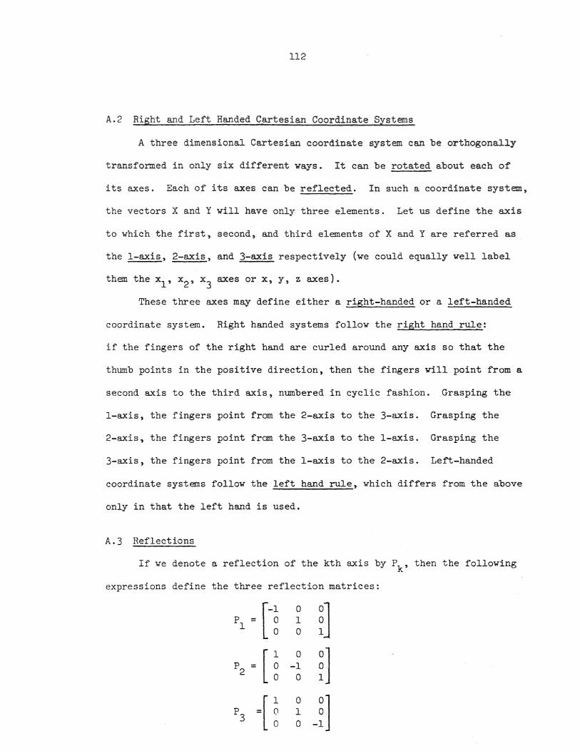
112
A.2 Right and Left Handed Cartesian Coordinate Systems
A three dimensional Cartesian coordinate system can be orthogonally
transformed in only six different ways. It can be rotated about each of
its axes. Each of its axes can be reflected. In such a coordinate system,
the vectors X and Y will have only three elements. Let us define the axis
to which the first, second, and third elements of X and Y are referred as
the 1-axis, 2-axis, and 3-axis respectively (we could equally well label
them the x1 , x2 , x3 axes or x, y, z axes).
These three axes may define either a right-handed or a left-handed
coordinate system. Right handed systems follow the right hand rule:
if the fingers of the right hand are curled around any axis so that the
thumb points in the positive direction, then the fingers will point from a
second axis to the third axis, numbered in cyclic fashion. Grasping the
1-axis, the fingers point from the 2-axis to the 3-axis. Grasping the
2-axis, the fingers point from the 3-axis to the 1-axis. Grasping the
3-axis, the fingers point from the 1-axis to the 2-axis. Left-handed
coordinate systems follow the left hand rule, which differs from the above
only in that the left hand is used.
A.3 Reflections
If we denote a reflection of the kth axis by Pk, then the following
expressions define the three reflection matrices:
l~ 0
~] pl = 1 0
= [ 1 0
~] p2 0 -1 0 0
=[ 1 0
-~J p3 0 1 0 0

113
Note that reflection_matrices commute (e.g. P2P3 = P3P2 ), so that it
makes no difference in what order a sequence of reflections are performed.
Note also that an odd number of reflections changes the handedness of the
coordinate system.
A.4 Rotations
th If we denote a rotation of angle e about the k axis by Rk(e),
then the following expressions define the three rotation matrices:
R1 (e) ·U e [cos
R2(e) = ~ e s1.n
{ cos e
-sin e 0
0 cos e
-sin e
0 1 0
sin e cos e
0
0
~ sin cos
-sin
J 0 cos
Note that rotation matrices do not commute. The product of several
rotations is performed from right to left, for examrle in
the rotations are performed about the 3-axis of the original system, the
2-axis of the transformed system, and the 1-axis of the doubly transformed
system, to yield the final triply transformed system.
If the rotation angles are all so small that their cosines can be
assumed to be unity, then the rotation matrices become commutative. This
is the case for differential rotations, for example.
The above expressions define positive rotations, which are right-
hand rotations for right-handed coordinate systems and left-hand rotations

114
for left-handed coordinate systems. A right-hand rotation is related to
the right hand rule given above: if the fingers of the right hand are
curled around the rotation axis so that the thumb points in the positive
direction» then the fingers curl in the direction of a right hand rotation.
A similar statement for left hand rotations is obvious.
A.5 Inverse Transformations ~
The inverse of a transformation A (denoted A-~) is the transformation
which returns conditions to their original state, that is
Re£1ections are self-inverse, that is
Common sense tells us that the inverse of a positive rotation is a
negative rotation, that is
R~1 (e) = Rk(-e)
and this conclusion is verified by taking the orthogonal property
AT A = I
from which it is evident that for orthogonal matrices
and for each of the above expressions for rotation matrices it can be shown that
we have
Applying the rule for the inverse of products
[A B)-l = B-l A-l

115
A product transformation consisting of one rotation and one
reflection commutes only if the rotation and reflection refer to the same
axis, that is
if j = k
otherwise
if j 1 k.