cooperative target tracking using mobile robots -...
TRANSCRIPT

Cooperative Target Tracking using Mobile Robots
Ph.D. Dissertation Proposalsubmitted by
Boyoon Jung
February 2004
Guidance Committee
Gaurav S. Sukhatme (Chairperson)Maja J. MataricMilind TambeIsaac CohenKwan Min Lee (Outside Member)

Abstract
We study the problem of multiple target tracking using multiple mobile robots. Our approach
is to divide the cooperative multi-target tracking problem into two sub-problems: target tracking
using a single mobile robot and on-line motion strategy design for multi-robot coordination.
For single robot-based tracking, we address two key challenges: how to separate the ego-
motion of the robot from the motions of external objects, and how to compensate this ego-motion
to detect and track moving objects robustly. An ego-motion compensation method using salient
feature tracking is described, and the design of a probabilistic filter to handle the noise and uncer-
tainty of sensor inputs is presented. The proposed method is implemented and tested in various
outdoor environments using three different robot platforms: a robotic helicopter, a Segway RMP,
and a Pioneer2 AT, which have unique ego-motion characteristics.
For multi-robot coordination, we propose an algorithm based on treating the densities of
robots and targets as properties of the environment in which they are embedded. By suitably
manipulating these densities a control law for each robot is proposed. We term our approach
Region-based, and describe and validate it through an example. We observe that the general
approach can be significantly improved in the special case where the topology of the environment
is known in advance. We derive a specialized version of the control law for this case; the resulting
algorithm is called the Topological Region-Based Approach. We also give the formulation of the
solution in the unstructured case, termed the Grid Region-Based Approach. These coordination
approaches have been implemented in simulation, and in real robot systems. Experiments indicate
that our treatment of the coordination problem based on environmental characteristics is effective
and efficient.
There are four additional topics we plan to address for the final thesis. First, sensor fusion
techniques will be studied for target position estimation in 3D space. The current single-robot
tracker integrates laser range scans into the estimation system by simply projecting the scans into
the 2D image space, which causes poor estimation results when a robot turns at high velocity.
Second, the stability properties of the Region-based Approach will be analyzed theoretically and
through simulations. The system’s behavior in response to static or oscillating target motions
will be studied. Third, the performance of the Grid Region-based Approach will be tested and
ii

characterized through intensive simulations with various configurations in order to investigate the
effect of environmental structure, broken inter-robot communication links, and increased target
population. Finally, all system components will be integrated, and tracking experiments in an
outdoor setting using multiple robots will be performed to test the robustness of the entire system.
iii
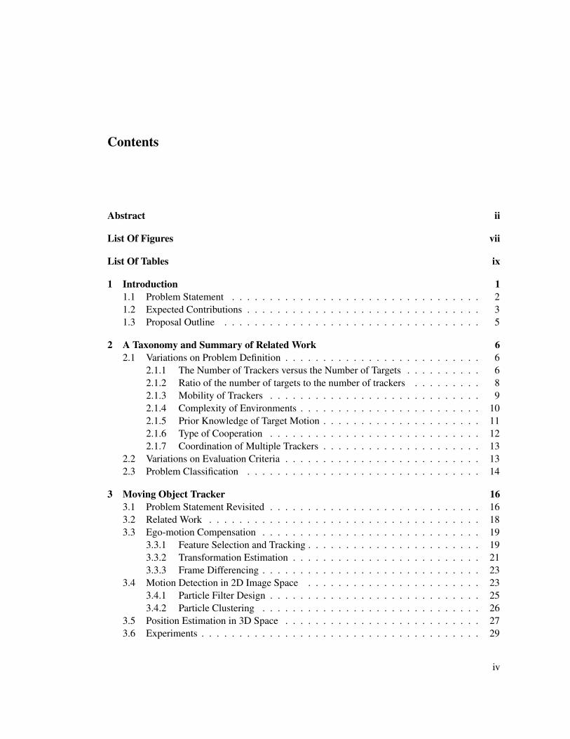
Contents
Abstract ii
List Of Figures vii
List Of Tables ix
1 Introduction 11.1 Problem Statement . . . . . . . . . . . . . . . . . . . . . . . . . . . . . . . . . 21.2 Expected Contributions . . . . . . . . . . . . . . . . . . . . . . . . . . . . . . . 31.3 Proposal Outline . . . . . . . . . . . . . . . . . . . . . . . . . . . . . . . . . . 5
2 A Taxonomy and Summary of Related Work 62.1 Variations on Problem Definition . . . . . . . . . . . . . . . . . . . . . . . . . . 6
2.1.1 The Number of Trackers versus the Number of Targets . . . . . . . . . . 62.1.2 Ratio of the number of targets to the number of trackers . . . . . . . . . 82.1.3 Mobility of Trackers . . . . . . . . . . . . . . . . . . . . . . . . . . . . 92.1.4 Complexity of Environments . . . . . . . . . . . . . . . . . . . . . . . . 102.1.5 Prior Knowledge of Target Motion . . . . . . . . . . . . . . . . . . . . . 112.1.6 Type of Cooperation . . . . . . . . . . . . . . . . . . . . . . . . . . . . 122.1.7 Coordination of Multiple Trackers . . . . . . . . . . . . . . . . . . . . . 13
2.2 Variations on Evaluation Criteria . . . . . . . . . . . . . . . . . . . . . . . . . . 132.3 Problem Classification . . . . . . . . . . . . . . . . . . . . . . . . . . . . . . . 14
3 Moving Object Tracker 163.1 Problem Statement Revisited . . . . . . . . . . . . . . . . . . . . . . . . . . . . 163.2 Related Work . . . . . . . . . . . . . . . . . . . . . . . . . . . . . . . . . . . . 183.3 Ego-motion Compensation . . . . . . . . . . . . . . . . . . . . . . . . . . . . . 19
3.3.1 Feature Selection and Tracking . . . . . . . . . . . . . . . . . . . . . . . 193.3.2 Transformation Estimation . . . . . . . . . . . . . . . . . . . . . . . . . 213.3.3 Frame Differencing . . . . . . . . . . . . . . . . . . . . . . . . . . . . . 23
3.4 Motion Detection in 2D Image Space . . . . . . . . . . . . . . . . . . . . . . . 233.4.1 Particle Filter Design . . . . . . . . . . . . . . . . . . . . . . . . . . . . 253.4.2 Particle Clustering . . . . . . . . . . . . . . . . . . . . . . . . . . . . . 26
3.5 Position Estimation in 3D Space . . . . . . . . . . . . . . . . . . . . . . . . . . 273.6 Experiments . . . . . . . . . . . . . . . . . . . . . . . . . . . . . . . . . . . . . 29
iv

3.6.1 Experimental Setup . . . . . . . . . . . . . . . . . . . . . . . . . . . . . 293.6.2 Experimental Results . . . . . . . . . . . . . . . . . . . . . . . . . . . . 30
3.7 Discussion . . . . . . . . . . . . . . . . . . . . . . . . . . . . . . . . . . . . . . 35
4 Cooperative Multi-Target Tracking 364.1 Problem Statement Revisited . . . . . . . . . . . . . . . . . . . . . . . . . . . . 364.2 Related Work . . . . . . . . . . . . . . . . . . . . . . . . . . . . . . . . . . . . 374.3 Region-based Approach . . . . . . . . . . . . . . . . . . . . . . . . . . . . . . . 38
4.3.1 Relative Density Estimates as Attributes of Space . . . . . . . . . . . . . 394.3.2 Urgency Distribution and Utility . . . . . . . . . . . . . . . . . . . . . . 434.3.3 Distributed Motion Strategy . . . . . . . . . . . . . . . . . . . . . . . . 44
4.4 Grid Region-Based Approach . . . . . . . . . . . . . . . . . . . . . . . . . . . . 464.4.1 Virtual Region Representation and Density Estimates . . . . . . . . . . . 464.4.2 Estimation of the Utility Distribution . . . . . . . . . . . . . . . . . . . 474.4.3 Motion Strategy for Cooperative Target Tracking . . . . . . . . . . . . . 48
4.5 Topological Region-based Approach . . . . . . . . . . . . . . . . . . . . . . . . 504.5.1 Density Estimates on a Topological Map . . . . . . . . . . . . . . . . . 504.5.2 The Coarse Deployment Strategy . . . . . . . . . . . . . . . . . . . . . 514.5.3 Target Tracking within a Region . . . . . . . . . . . . . . . . . . . . . . 52
4.6 Discussion . . . . . . . . . . . . . . . . . . . . . . . . . . . . . . . . . . . . . . 53
5 Experiments in Structured Environments 545.1 System Design and Implementation . . . . . . . . . . . . . . . . . . . . . . . . 54
5.1.1 The Motor Actuation Layer . . . . . . . . . . . . . . . . . . . . . . . . 545.1.2 The Target Tracking Layer . . . . . . . . . . . . . . . . . . . . . . . . . 565.1.3 Monitoring Layer . . . . . . . . . . . . . . . . . . . . . . . . . . . . . . 56
5.2 Experimental Setup . . . . . . . . . . . . . . . . . . . . . . . . . . . . . . . . . 575.2.1 Target Modeling . . . . . . . . . . . . . . . . . . . . . . . . . . . . . . 585.2.2 Environment Complexity . . . . . . . . . . . . . . . . . . . . . . . . . . 585.2.3 Experiment Design . . . . . . . . . . . . . . . . . . . . . . . . . . . . . 60
5.2.3.1 Region-based versus Local-following Strategy . . . . . . . . . 605.2.3.2 Robot Density versus Visibility . . . . . . . . . . . . . . . . . 615.2.3.3 Mobile Robots versus Embedded Sensors . . . . . . . . . . . 61
5.3 Experimental Results . . . . . . . . . . . . . . . . . . . . . . . . . . . . . . . . 625.3.1 Region-based versus Local-following Strategy . . . . . . . . . . . . . . 625.3.2 Robot Density versus Visibility . . . . . . . . . . . . . . . . . . . . . . 625.3.3 Mobile Robots versus Embedded Sensors . . . . . . . . . . . . . . . . . 62
5.4 Discussion . . . . . . . . . . . . . . . . . . . . . . . . . . . . . . . . . . . . . . 655.4.1 Region-based versus Local-following Strategy . . . . . . . . . . . . . . 655.4.2 Robot Density versus Visibility . . . . . . . . . . . . . . . . . . . . . . 665.4.3 Mobile Robots versus Embedded Sensors . . . . . . . . . . . . . . . . . 675.4.4 Summary . . . . . . . . . . . . . . . . . . . . . . . . . . . . . . . . . . 67
v

6 Experiments in Unstructured Environments 696.1 System Design and Implementation . . . . . . . . . . . . . . . . . . . . . . . . 69
6.1.1 Motion Tracker . . . . . . . . . . . . . . . . . . . . . . . . . . . . . . . 696.1.2 Localization . . . . . . . . . . . . . . . . . . . . . . . . . . . . . . . . . 696.1.3 Cooperative Motion Planning . . . . . . . . . . . . . . . . . . . . . . . 716.1.4 Navigation . . . . . . . . . . . . . . . . . . . . . . . . . . . . . . . . . 72
6.2 Experimental Setup . . . . . . . . . . . . . . . . . . . . . . . . . . . . . . . . . 726.3 Experimental Results . . . . . . . . . . . . . . . . . . . . . . . . . . . . . . . . 736.4 Discussion . . . . . . . . . . . . . . . . . . . . . . . . . . . . . . . . . . . . . . 74
7 Conclusion and Future Work 777.1 Research Plan . . . . . . . . . . . . . . . . . . . . . . . . . . . . . . . . . . . . 78
Reference List 80
Appendix AList of Publications . . . . . . . . . . . . . . . . . . . . . . . . . . . . . . . . . . . . 89A.1 Refereed Journal Papers . . . . . . . . . . . . . . . . . . . . . . . . . . . . . . 89A.2 Refereed Conference Papers . . . . . . . . . . . . . . . . . . . . . . . . . . . . 89A.3 Unrefereed Technical Reports . . . . . . . . . . . . . . . . . . . . . . . . . . . 90
Appendix BExtension: Visibility Maximization . . . . . . . . . . . . . . . . . . . . . . . . . . . . 91
vi

List Of Figures
1.1 Cooperation among multiple robots . . . . . . . . . . . . . . . . . . . . . . . . 3
1.2 Multiple Target Tracking using Multiple Robots . . . . . . . . . . . . . . . . . . 4
2.1 Research in target tracking problem . . . . . . . . . . . . . . . . . . . . . . . . 15
3.1 Multiple Target Tracking using a Single Robot . . . . . . . . . . . . . . . . . . . 17
3.2 Processing sequence for moving object tracking from a mobile robot . . . . . . . 18
3.3 Salient features selected for tracking . . . . . . . . . . . . . . . . . . . . . . . . 20
3.4 Feature tracking . . . . . . . . . . . . . . . . . . . . . . . . . . . . . . . . . . . 21
3.5 Outlier feature detection . . . . . . . . . . . . . . . . . . . . . . . . . . . . . . 22
3.6 Image Transformation . . . . . . . . . . . . . . . . . . . . . . . . . . . . . . . . 24
3.7 Results of frame differencing . . . . . . . . . . . . . . . . . . . . . . . . . . . . 24
3.8 Particle filter tracking . . . . . . . . . . . . . . . . . . . . . . . . . . . . . . . . 27
3.9 Projection of laser scans onto the image coordinates . . . . . . . . . . . . . . . . 28
3.10 Projected laser scans . . . . . . . . . . . . . . . . . . . . . . . . . . . . . . . . 29
3.11 Robot platforms for experiments . . . . . . . . . . . . . . . . . . . . . . . . . . 30
3.12 Snapshots of particle filter tracking a moving object: from Robotic helicopter . . 31
3.13 Snapshots of particle filter tracking a moving object: from Segway RMP . . . . . 32
3.14 Snapshots of particle filter tracking a moving object: from Pioneer2 AT . . . . . 32
3.15 Performance evaluation: tracking from Robotic helicopter . . . . . . . . . . . . 33
3.16 Performance evaluation: tracking from Segway RMP . . . . . . . . . . . . . . . 33
3.17 Performance evaluation: tracking from Pioneer2 AT . . . . . . . . . . . . . . . . 34
4.1 Positions of mobile robots and targets in a bounded environment . . . . . . . . . 39
4.2 Robot distribution model . . . . . . . . . . . . . . . . . . . . . . . . . . . . . . 40
4.3 Target distribution model . . . . . . . . . . . . . . . . . . . . . . . . . . . . . . 41
4.4 Region models for density computation . . . . . . . . . . . . . . . . . . . . . . 41
4.5 Robot density distribution . . . . . . . . . . . . . . . . . . . . . . . . . . . . . . 42
4.6 Target density distribution . . . . . . . . . . . . . . . . . . . . . . . . . . . . . 43
4.7 Urgency distribution . . . . . . . . . . . . . . . . . . . . . . . . . . . . . . . . 44
vii

4.8 Example of a cost function . . . . . . . . . . . . . . . . . . . . . . . . . . . . . 45
4.9 Utility distribution . . . . . . . . . . . . . . . . . . . . . . . . . . . . . . . . . 45
4.10 Parameterized virtual region . . . . . . . . . . . . . . . . . . . . . . . . . . . . 47
4.11 Snapshot of the utility distribution . . . . . . . . . . . . . . . . . . . . . . . . . 49
4.12 Example of a topological map . . . . . . . . . . . . . . . . . . . . . . . . . . . 50
4.13 Following targets within a region . . . . . . . . . . . . . . . . . . . . . . . . . . 53
5.1 Behavior-based robot control architecture . . . . . . . . . . . . . . . . . . . . . 55
5.2 Configurations for robots and targets . . . . . . . . . . . . . . . . . . . . . . . . 57
5.3 System architecture for targets . . . . . . . . . . . . . . . . . . . . . . . . . . . 58
5.4 The simulation environments . . . . . . . . . . . . . . . . . . . . . . . . . . . . 59
5.5 Environment for real-robot experiments . . . . . . . . . . . . . . . . . . . . . . 62
5.6 Simulation results comparing the performance of the two strategies . . . . . . . . 63
5.7 Performance with visibility maximization . . . . . . . . . . . . . . . . . . . . . 64
5.8 Performance of the real-robot system . . . . . . . . . . . . . . . . . . . . . . . . 64
5.9 Tracking examples . . . . . . . . . . . . . . . . . . . . . . . . . . . . . . . . . 68
6.1 System architecture for Grid Region-based Approach . . . . . . . . . . . . . . . 70
6.2 Robot localization using Kalman filters . . . . . . . . . . . . . . . . . . . . . . 71
6.3 Navigation using the VFH+ algorithm . . . . . . . . . . . . . . . . . . . . . . . 73
6.4 Virtual region selection behavior . . . . . . . . . . . . . . . . . . . . . . . . . . 74
6.5 Region-switching behavior . . . . . . . . . . . . . . . . . . . . . . . . . . . . . 76
B.1 Coverage computation . . . . . . . . . . . . . . . . . . . . . . . . . . . . . . . 91
B.2 Visibility maximization method relying on local sensing . . . . . . . . . . . . . 92
viii

List Of Tables
3.1 Adaptive Particle Filter Algorithm . . . . . . . . . . . . . . . . . . . . . . . . . 26
3.2 Expectation-Maximization Algorithm for Particle Clustering . . . . . . . . . . . 28
3.3 Performance of moving object detection algorithm . . . . . . . . . . . . . . . . 34
5.1 Complexity of the environments as a function of number of targets . . . . . . . . 60
5.2 Significance values from T-test as a function of number of targets and environ-ment characteristic . . . . . . . . . . . . . . . . . . . . . . . . . . . . . . . . . 65
5.3 Significance values from T-test as a function of number of targets and differentstrategies . . . . . . . . . . . . . . . . . . . . . . . . . . . . . . . . . . . . . . 66
7.1 Timetable for future work . . . . . . . . . . . . . . . . . . . . . . . . . . . . . . 79
ix

Chapter 1
Introduction
The target tracking problem is to estimate the state of a target1 based on inaccurate measurements
from sensors. The estimation process contains many uncertainties; for example, the measure-
ments are corrupted by noise, the origin of the measurements are unauthenticated, the motion of
the target is unknown, etc. The roots of the target tracking problem go back to World War II, when
automated systems to control anti-aircraft guns were developed, and algorithms were designed to
track aircraft using RADAR and predict their future positions. Present day applications of target
tracking algorithms range from automated surveillance to security systems, which require the ca-
pability of tracking the positions of multiple targets (eg. people in a building) autonomously and
effectively.
The target tracking problem has been studied in diverse research areas with many applications
in mind. Traditionally, the signal processing community (Bar-Shalom, 1992; Biernson, 1990;
Blackman, 1986; Bogler, 1990; Kolawole, 2002; Siouris et al., 1997) has designed probabilistic
filters to track missiles or vehicles using RADAR for mainly military purposes. The computer
vision community (Behrad et al., 2001; Cohen and Medioni, 1999; Foresti and Micheloni, 2003;
Kang et al., 2002; Koyasu et al., 2001; Lipton et al., 1998; Murray and Basu, 1994) has developed
algorithms to track visual targets using camera(s), and the sensor network community (Guibas,
2002; Horling et al., 2001; Li et al., 2002; Liu et al., 2002; Moore et al., 2003; Zhao et al., 2002)
has utilized deployed sensors to monitor moving objects in an environment.
We are interested in tracking targets using mobile robots as the tracking devices. Using a
group of mobile robots for target tracking is beneficial because:
1. A mobile robot can cover a wide area over time, which means the number of sensors
required for tracking can be kept small.
1In this thesis, we assume that a target is a moving object and its state is its location.
1
2. A mobile robot can re-position itself in response to the movement of the targets for efficient
tracking.
When the number of targets is much bigger than the number of sensors available or when sensors
cannot be deployed in advance, the mobility of sensors become indispensable. For surveillance
and security applications, multiple robots can be used for efficient monitoring; this requires a
coordinated motion strategy for cooperative tracking.
The motion tracking and estimation of moving objects in the vicinity of a mobile robot is
also a fundamental capability for safe navigation. Populated environments are challenging to
contemporary mobile robots. One of the main reasons is the presence of dynamic objects, whose
motions are diverse (eg. due to pedestrians, bicycles, automobiles, etc). Since some objects
move faster than the robot, motion detection and estimation for potential collision avoidance are
the most fundamental skills that a robot needs to function effectively in dynamic environments.
Needless to say, target tracking is a key enabler for robust motion estimation.
This thesis addresses the development of a multiple target tracking system using multiple mo-
bile robots. Intuitively tracking performance can be improved by exploiting multiple robots, and
cooperation among the robots is the key point to take advantage of the multi-robot system. There
are two expected improvements attributable to multi-robot cooperation. The uncertainty of target
position estimation can be reduced by combining measurements from multiple robots (Spletzer
and Taylor, 2003; Stroupe et al., 2001). In this case, the motion strategy of each robot is to
minimize the redundant measurement uncertainty; for example, when the horizontal and verti-
cal uncertainties of a single-robot measurement are different, two robots can minimize the total
estimation error by positioning themselves so that their headings are orthogonal to each other
(Figure 1.1 (a)). As the other possible improvement, the total number of tracked targets over time
can be maximized by distributing robots properly and allocating targets to a robot in the best po-
sition (Jung and Sukhatme, 2002; Parker, 1999; Werger and Mataric, 2000). The motion strategy
of robots for this case is to minimize the redundant target allocation; for example, each target
would be allocated to a robot in the best position according to the tracking range, which stops
multiple robots from tracking the same target. Both cases require that the amount of exchanged
information among robots should be minimized, and the collective data should be simple enough
to be processed in real-time. We focus on the latter type of cooperation.
1.1 Problem Statement
The multiple target tracking problem using multiple mobile robots is defined as follows.
2

(a) Uncertainty reduction (b) Target allocation
Figure 1.1: Cooperation among multiple robots: The uncertainty of estimation can be reduced bycombining multiple measurements, or the total number of tracked targets can be maximized byallocating each target to a robot in the best pose.
Input Multiple mobile robots and multiple targets in an environment
Output Positions of detected targets in a global coordinate system
Goal To maximize the number of tracked targets over time
Restriction No prior knowledge of the number of robots, the number of targets, or
a target motion model
A decomposition of the problem is shown in Figure 1.2. The system consists of M robots and
N targets, and the available measurements are sensor data for robot localization (eg. GPS, IMU,
and odometry) and target detection and tracking (eg. camera and laser rangefinder). Since the
multi-robot system has no control over target motions, the only factor to maximize the number of
tracked targets is each robot’s motion control. Based on the current poses of mobile robots and
the current positions of targets, each robot infers the best new position to move toward, in order
to maximize the number of tracked targets over time.
Our design goal is to develop a hierarchical system by decoupling the (low-level) target-
tracking algorithm and the (high-level) cooperation strategy. The low-level tracking algorithm
focuses on the single-robot, multiple-target problem so that an individual robot performs robust
target tracking. On top of the low-level capability, an on-line, coordinated motion strategy is
developed for robot positioning in distributed manner, resulting in a solution to the multi-robot
tracking problem.
1.2 Expected Contributions
Here we outline the significant contributions presented in the thesis.
3

Figure 1.2: Multiple Target Tracking using Multiple Robots: The problem can be decomposedinto three sub-problems: robot localization, target tracking, and cooperation.
1. The taxonomy of the target tracking problem, presented in Chapter 2.
The target tracking problem has been studied by diverse research communities in differ-
ent perspectives for various applications. We provide a taxonomy that classifies previous
research according to the variants of the problem definitions and evaluation criteria. For
each cluster within this classification, the main research issues and related literature are
described.
2. Moving object tracker design and its experimental evaluation, presented in Chapter 3.
We address two key challenges for single robot-based moving object tracking: how to
separate the ego-motion of the robot from the motions of external objects, and how to com-
pensate this ego-motion to detect and track moving objects. An ego-motion compensation
method using salient feature tracking is described, and the design of a probabilistic filter
to handle the noise and uncertainty of sensor inputs is presented. The proposed method is
implemented and tested in various outdoor environments using three different robot plat-
forms, which have unique ego-motion characteristics.
3. New mechanism for cooperative tracking using multiple robots, presented in Chap-ter 4.
We propose an algorithm for multi-robot coordination with applications to multiple target
tracking. The proposed algorithm treats the densities of robots and targets as properties of
the environment in which they are embedded, and a control law for each robot is generated
by suitably manipulating these densities. Since the proposed mechanism is distributed and
4

expandable, it can be applied for various sensor configurations. For example, a heteroge-
nous sensor network can adopt the mechanism with minimal modification, and sensors can
be added to (or subtracted from) a tracking network on the fly without stopping operation.
Experiments indicate that our treatment of the coordination problem based on environmen-
tal characteristics is effective and efficient.
4. Introduction of an environmental complexity metric for tracking performance analysis,presented in Section 5.2.2.
In structured environments, we exploit the topology of the environment to optimize track-
ing, so the structure and complexity of an environment has an indirect effect on the overall
tracking performance. A method to measure the complexity of an environment is presented,
and the influence of environmental structure on tracking is experimentally verified.
5. Demonstration of possible improvement by constructing a sensor network using mo-bile and stationary sensors, presented in Section 5.2.3.3.
Both mobile and stationary trackers have their own advantages. For example, a mobile
tracker can cover wider area over time, and can adapt to targets’ movement patterns. On
the other hand, a stationary tracker can be installed at the best position depending on the
environments, and cause less interference. We demonstrate that performance improvement
is expected by constructing a sensor network with both kinds of trackers.
1.3 Proposal Outline
This thesis proposal is organized as follows. Chapter 2 provides a summary of previous research.
The tracking problem has been studied in diverse areas; we categorize related work based on
problem definition and evaluation criteria. Chapter 3 describes our approach for a moving-object
tracker using a single robot. There are two independent motions involved: motions of moving
objects and the ego-motion of the robot. The ego-motion is compensated for motion detection
and tracking. Chapter 4 presents our cooperation mechanism for multiple target tracking using
multiple mobile robots. The general idea is described first, and two implementations for differ-
ent environments are described. In Chapter 5 the experimental results from a structured indoor
environment are discussed; the experimental results for an unstructured outdoor environment are
analyzed in Chapter 6. Finally, the current status and plans for thesis completion are discussed in
Chapter 7.
5

Chapter 2
A Taxonomy and Summary of Related Work
The target tracking problem has been studied by various research groups from different points of
view. Even though the basic concept of estimating the position of an interesting object remains
same, the detailed problem definition or approaches are different. As a way of differentiating our
work from previous research, we present a taxonomy that classifies tracking research according
to the various problem definitions and evaluation criteria.
2.1 Variations on Problem Definition
The target tracking problems can be classified along multi-dimensions. There are several natural
dimensions, for example, the number of trackers1, the number of targets, the mobility of trackers,
etc.
2.1.1 The Number of Trackers versus the Number of Targets
The most natural classification axis is the number of trackers, and the axis can be divided into
’single’ or ’multiple’ based on whether cooperation among trackers is planned or not. Even
when there are multiple trackers involved in a system, we consider it as a single tracker problem
if there is no cooperation among the trackers. Another obvious axis is the number of targets,
which affects the complexity of data association problem2 or multi-tracker cooperation strategy.
1In some papers (Bar-Shalom, 1990) the general term, sensor, is used to describe an elemental tracking device.The terminology is appropriate when each sensor returns a partial or full state measurement of a target. For example,a RADAR sensor returns a 2 dimensional position information of a target, and the sensor is a tracker. However, itbecomes confusing when there are sensors in the system whose measurements provide no information of target state.For example, when a mobile robot equipped with a camera and a GPS sensor is used for a target tracking in the globalcoordinate system, the GPS sensor is not a tracker because it measures only the robot state. In this case, a mobile robotis a tracker. Therefore, we use the collective term, tracker to indicate an elemental tracking device.
2The data association problem is to find the origin of measurements. Even for a single target case, the dataassociation problem (eg. does a measurement originate from a target or noise?) needs to be solved, but when there are
6

A tracking problem can be classified under one of the following four categories according to the
combination of these two axes.
Single Tracker Single Target (STST) A single tracker is used to track a single target. Most
work in this category focuses on signal processing techniques for target detection, prob-
abilistic filter design to filter out noisy measurements, and failure recovery. The Kalman
filter (Bar-Shalom and Fortmann, 1988; Biernson, 1990; Bogler, 1990) and the particle fil-
ter (Gustafsson et al., 2002; Isard and Blake, 1998) have been applied to the single target
tracking problem successfully. Liu and Fu (2001) proposed the Probabilistic Data Associa-
tion (PDA) filter to achieve successful tracking in cluttered environments. Chung and Yang
(1995); Coue and Bessiere (2001) presented visual servoing techniques to track a target,
and Fabiani et al. (2002); LaValle et al. (1997); Murrieta-Cid et al. (2002) introduced the
motion strategy of a mobile robot maintaining visibility of a moving target in a cluttered
workspace. Many efforts (Behrad et al., 2001; Foresti and Micheloni, 2003; Murray and
Basu, 1994; Nordlund and Uhlin, 1996; Yilmaz et al., 2001) to detect and track a visual
target using a single camera come from the computer vision community.
Single Tracker Multiple Targets (STMT) A single tracker is used to track multiple targets.
The research in this category focuses on data association and target identification. Cox
and Hingorani (1996); Danchick and Newnam (1993); Reid (1979) presented the Multiple
Hypothesis Tracking (MHT) algorithm and its application to visual tracking. Bar-Shalom
and Fortmann (1988); Fortmann et al. (1983) introduced the Joint Probabilistic Data As-
sociation Filter (JPDAF) that computes the probabilities of measurement association to the
multiple targets, and Frank (2003); Schultz et al. (2001) extended it using a sample-based
method. Carine Hue and Perez (2002); Herman (2002); Meier and Ade (1999); Monte-
merlo et al. (2002); Orton and Fitzgerald (2002) demonstrated how the particle filter can be
exploited for the data association problem. Cohen and Medioni (1999) utilized a graph rep-
resentation to store template information of moving objects, and solved the data association
problem by searching an optimal path in the graph.
Multiple Trackers Single Target (MTST) A single target is tracked by multiple trackers. The
main issue in this category is how to combine multiple measurements from multiple track-
ers to improve the estimation accuracy. Dana (1990); Kang et al. (2002) described regis-
tration procedure that projects sensory data from multiple sources into a common global
multiple targets involved, the uncertainty of measurement origin increases drastically because a measurement couldoriginate from one of many targets, or from noisy input.
7

coordinate system, and Brooks and Williams (2003); Maybeck et al. (1994); Wilhelm et al.
(2002) presented target-tracking systems that fuse two estimates from heterogeneous track-
ers for better accuracy or robustness. Stroupe et al. (2001) demonstrated that the accuracy
of ball tracking was improved by combining data from multiple robots, and Spletzer and
Taylor (2003) presented a control strategy to move multiple robots to the optimal positions
so that the estimation uncertainty of target position is minimized. Most target tracking re-
search using a sensor network (Horling et al., 2001; Li et al., 2002; Liu et al., 2002; Moore
et al., 2003; Zhao et al., 2002) falls under this category.
Multiple Trackers Multiple Targets (MTMT) Multiple trackers are used to track multiple tar-
gets cooperatively. The research focuses on how to combine multiple measurements and
solve the association problem at the same time, how to position trackers to track more tar-
gets, or how many trackers are required for a given environment and targets. Blackman
(1990); Chong et al. (1990) outlined the issues and the methods related to the fusion of
multiple sensor data or the association of multiple tracks. Gerkey and Mataric (2001);
Jung and Sukhatme (2002); Parker (1999); Werger and Mataric (2000) proposed various
multi-robot motion strategies to maximize the number of targets over time. Guibas et al.
(1997); Yamashita et al. (1997) introduced a few theoretical bounds on how many trackers
are necessary and sufficient to search well-defined environments (eg. polygonal region or
simply-connected free space).
This thesis presents a solution for the MTMT problem when trackers are mobile robots. In con-
trast to other approaches, the presented solution decouples the low-level tracking and the high-
level cooperation for simplicity. Note that the low-level tracking is simply the STMT problem.
2.1.2 Ratio of the number of targets to the number of trackers
There is another classification axis related to the number of trackers and targets, the ratio r of the
number of targets to the number of trackers. For the MTST and MTMT problem, this ratio is one
of the characteristics that influences the solution approaches.
r � 1.0 The extreme case in this category is a sensor network (Horling et al., 2001; Li et al.,
2002; Liu et al., 2002; Moore et al., 2003; Zhao et al., 2002), which assumes a very large
number of sensors spread in an environment and few objects in it. Each sensor has limited
capability and its measurement contains high uncertainty (eg. distant measurement only
or existence in a certain range only), and the tracking is performed by triangulating or
8

overlapping multiple measurements. Also, most MTST problems (Dana, 1990; Spletzer
and Taylor, 2003; Stroupe et al., 2001) fall under this category.
r ≈ 1.0 When there are enough trackers available to track all targets, the tracking problem can
be treated as a task allocation problem (Gerkey and Mataric, 2001; Parker, 1999; Werger
and Mataric, 2000). Based on the current positions of trackers and targets, each target is
allocated to each tracker to improve overall tracking performance.
r � 1.0 When the number of trackers is not big enough to track all targets (Jung and Sukhatme,
2002), trackers are allocated according to spatial density rather than to targets themselves.
Research on how to characterize space based on target positions and how to position track-
ers based on these characteristics are the main issues.
This thesis focuses the third case when the number of targets is much bigger than the number of
trackers, which implies cooperation among trackers is indispensable.
2.1.3 Mobility of Trackers
Perhaps the most interesting axis for roboticists is the mobility of trackers. Based on the degree
of possible tracker motions, we classify the tracking problem as stationary, pan/tilt/zoom, planar,
and unrestricted.
Stationary Since there is no motion control involved in this category, most work focuses on
reliable perception. Biernson (1990); Bogler (1990); Kolawole (2002) presented RADAR-
based trackers, and Haritaoglu et al. (1998); Kang et al. (2002); Lipton et al. (1998) de-
scribed visual target trackers using a single or multiple stationary cameras. Sonars (Fort-
mann et al., 1983) and laser rangefinders (Brooks and Williams, 2003; Fod et al., 2002) are
also utilized to track targets.
Pan/Tilt/Zoom The Pan/Tilt/Zoom motion does not allow the tracker to move. Such trackers
extend the field and range of sensing, but have intrinsic limitations caused by the fixed
center position. Foresti and Micheloni (2003); Murray and Basu (1994) describe a target
tracking system using a single PTZ camera, and Kang et al. (2003); Stillman et al. (1998)
presented a heterogeneous tracking system that consists of a stationary camera and a PTZ
camera.
Planar The motion of a tracker is planar. For example, a pointing-down camera mounted on an
airplane flying at a constant altitude(Cohen and Medioni, 1999; Gustafsson et al., 2002)
9
was used to construct a background model by mosaicking input images, or a mobile robot
with a planar scan device (eg. a sonar array or a SICK laser rangefinder) moving on a
flat surface (Kluge et al., 2001; Montemerlo et al., 2002; Schultz et al., 2001) can build a
2D map of an environment. In both cases, moving targets can be detected by comparing
measurements to the planar model of the environment.
Unrestricted There is no restriction on the tracker motion. A camera mounted on a mobile
robot (Chung and Yang, 1995; Coue and Bessiere, 2001; Jung and Sukhatme, 2004; Nord-
lund and Uhlin, 1996) and a forward-looking infrared (FLIR) sensor attached to an airborne
platform (Braga-Neto and Goutsias, 1999; Maybeck et al., 1994; Yilmaz et al., 2001) are
examples.
The target tracker described in the thesis is a mobile robot with a single camera and a laser
rangefinder. Three different robot platforms are utilized to test the robustness of our tracking
algorithm. The case of using the robot helicopter falls under the third category and the other
two cases fall under the fourth category. The detailed motion characteristics of the platforms are
explained in Section 3.6.1.
2.1.4 Complexity of Environments
The complexity of the environment is an important factor for system design, especially when
trackers are mobile since the interaction between trackers and the environment should be taken
into account. Even when trackers are stationary, a tracking system should be able to recover from
lost tracking due to occlusion caused by the structure of an environment.
Empty Space Brooks and Williams (2003); Parker (1999); Spletzer and Taylor (2003); Werger
and Mataric (2000) make the open space assumption and focus only on the interaction
among trackers and targets. Even though the assumption is not made explicitly, some
works (Murray and Basu, 1994; Nordlund and Uhlin, 1996; Wilhelm et al., 2002) do not
take occlusion into account for their system design, then we categorize them in this class.
Structured Space When the environment is structured (eg. office-type, indoor environment),
a tracking system can actively exploit the structure of the environment for target detec-
tion (Meier and Ade, 1999; Montemerlo et al., 2002; Schultz et al., 2001) or tracker motion
planning (Jung and Sukhatme, 2002; Murrieta-Cid et al., 2002). Also, Behrad et al. (2001);
van Leeuwen and Groen (2002) presented front-car tracking systems on a paved road, and
those works fall under this category since they utilized the characteristics of parallel lanes.
10

Unstructured Space When an environment is cluttered the environment is classified as unstruc-
tured. Most works using probabilistic filters (Bar-Shalom and Fortmann, 1988; Houles and
Bar-Shalom, 1989; Orton and Fitzgerald, 2002; Reid, 1979) treat occlusion caused by en-
vironmental structure as uncertainty in sensor measurements. Coue and Bessiere (2001);
Fabiani et al. (2002); LaValle et al. (1997); Spletzer and Taylor (2003) presented motion
strategies for mobile robot-based trackers that minimize the loss of tracking performance
in cluttered environments.
The cooperative tracking algorithm presented in this thesis is implemented with two different
level of discretization. The first case described in Section 4.4 assumes an unstructured space,
and treats the environmental structure as an obstacles. The second case described in Section 4.5
assumes a structured space and actively takes advantage of the environmental structure for multi-
robot coordination. The individual tracking algorithm in Chapter 3 assumes and runs in unstruc-
tured environments.
2.1.5 Prior Knowledge of Target Motion
Prior knowledge of targets’ motion is an important determinant since tracking solutions may be
different depending on the motions of targets (eg. random vs. predictable).
Deterministic The most well-known example in this category is the traditional missile tracking
problem (Kirubarajan et al., 2001; Siouris et al., 1997; Song et al., 1990). Since the tra-
jectory of a missile is governed by physics, future position can be inferred from a current
state. For example, the missile approach warning system (MAWS) (Difilippo and Camp-
bell, 1995) detects approaching missiles with enough warning time, and uses a determinis-
tic model of the target to compute the impact time and position. Spletzer and Taylor (2003)
discusses a multi-robot system that tracks an aerial target, whose motion was deterministic.
Probabilistic The prior knowledge of targets’ motion can be modeled with random variables.
For example, the motion of a maneuvering aircraft (Cooperman, 2002) or of a tactical bal-
listic missile (Vacher et al., 1992) cannot be captured using a single model. The interacting
multiple model (IMM) methods (Bar-Shalom et al., 1989; Blom and Bar-Shalom, 1988;
Houles and Bar-Shalom, 1989; Mazor et al., 1998) has been applied to those type of target
tracking problems; multiple dynamic models and their transition probabilities are designed
a priori, and a tracking system estimates not only the kinematic components but also the
11

best suitable model. Ikoma et al. (2002); McGinnity and Irwin (2001) presented sample-
based methods for model switching, and LaValle et al. (1997) computed optimal, numerical
solutions for a robot motion strategy when the target is predictable.
Unknown For real-world applications, the motion model of a target is often unavailable. In
such cases, there is no priori information about target movements, simple constant motion
models are utilized (Fod et al., 2002; Jung and Sukhatme, 2004; Kang et al., 2003; Koyasu
et al., 2001; Spletzer and Taylor, 2003). Montemerlo et al. (2002) assumed the Brownian
motion for a person’s typical movements to avoid estimating the velocity or acceleration of
a person.
The targets we attempt to track are any moving objects in the vicinity of a robot, and the motions
of the objects are diverse (eg. a person, a mobile robot, an automobile, etc.). Since there is no
assumption about the target variety, there is no prior information of target motions available. We
utilize a constant velocity model for robust tracking.
2.1.6 Type of Cooperation
For MTST and MTMT problems, cooperation among trackers is essential to improve tracking
performance, and two different types of improvement are expected:
Uncertainty Reduction The uncertainty of target position estimation can be reduced by com-
bining measurements from multiple trackers. Kang et al. (2002); Stillman et al. (1998)
demonstrated how the estimation error due to occlusion can be eliminated by using mul-
tiple cameras, and Brooks and Williams (2003); Wilhelm et al. (2002) presented tracking
systems that combines a visual tracker and a range tracker for better estimation. Splet-
zer and Taylor (2003); Stroupe et al. (2001) described multi-robot systems whose motion
strategy is to minimize the total estimation error.
Target Allocation The number of tracked targets over time can be maximized by distributing
trackers properly and allocating each target to a single tracker in the best position. Jung and
Sukhatme (2002); Parker (1999); Werger and Mataric (2000) presented cooperative motion
strategies for multi-robot systems, which attempt to minimize redundant target allocation.
In the ideal case every target is allocated to a single robot and every robot can track all
targets allocated to itself.
The goal of our research is to develop a control algorithm that deploys mobile robots according
to the target distribution so that the overall tracking performance is improved, which requires the
second type of cooperation.
12

2.1.7 Coordination of Multiple Trackers
When multiple trackers are used for target tracking and some of them have autonomy (eg. a target
tracking system using multiple mobile robots), a coordination strategy should be designed so that
the effect of cooperation can be maximized. The coordination strategy can be classified according
to whether or not the behavior of a tracker can be modified directly by other trackers’ decision.
Explicit One tracker can modify the behaviors of other trackers by explicit communication.
Werger and Mataric (2000) presented the Broadcast of Local Eligibility (BLE) technique; if
a particular robot thinks it is best suited to track a specified target, it stops other robots from
tracking the target by broadcasting inhibition signals over the network. Gerkey and Mataric
(2001) demonstrated that the target tracking problem can be solved using a principled pub-
lish/subscribe messaging model; the best capable robot is assigned to each tracking task
using a one-round auction.
Implicit All trackers make their own decision independently based on their best knowledge ac-
quired by exchanging information or observing others. Parker (1999) presented ALLIANCE
architecture to achieve target-assignment. If a robot was not able to track an assigned target
for a while, it would give up tracking the target. If a robot observes a target that has not
been tracked for a while, the robot would assign the target to itself. These behaviors are
achieved through the interaction of the motivational behavior; there is no explicit hand-
over mechanism.
There is no inhibition signal or two-way negotiation in our coordination method. Robots share
tracking information by broadcasting them, but the final decision is made independently, which
puts our work under the second category.
2.2 Variations on Evaluation Criteria
Tracking evaluation criteria vary from application to application; for example, a missile defence
system requires high accuracy of tracking results, but a surveillance system may prefer a tracking
system that can cover a wide area. Therefore, evaluation criteria are an important factor for
tracking system design.
Tracking Accuracy The most popular evaluation criterion is tracking accuracy. Since the target
tracking problem is to estimate the state of a target from noisy measurements, it is key
to filter out noise from measurements (Bar-Shalom and Fortmann, 1988; Biernson, 1990;
13

Bogler, 1990; Gustafsson et al., 2002; Isard and Blake, 1998), how to combine measure-
ments from multiple sources (Brooks and Williams, 2003; Dana, 1990; Kang et al., 2002;
Maybeck et al., 1994; Wilhelm et al., 2002), or how to distribute trackers to achieve better
accuracy (Spletzer and Taylor, 2003).
Collective Time Another popular evaluation criteria is the total collective time that targets are
tracked, which is proper to evaluate motion strategies of mobile tracking system. Especially
when the number of targets are bigger than the number of trackers and it is impossible to
track all targets all the time, the goal of a tracking system is often to maximize the number
of tracked targets over time (Jung and Sukhatme, 2002; Parker, 1999; Werger and Mataric,
2000).
Energy Efficiency For target tracking using a sensor network, power consumed in transmitting
or receiving messages for cooperation is a reasonable norm (Moore et al., 2003; Xu and
Lee, 2003; Zhang and Cao, 2004) since energy is the most limited resource of wireless
sensor nodes.
Travel Distance When trackers are mobile and the goal of the system is to track targets in
bounded environments, the total travel distance of a tracker can be used for performance
evaluation assuming a tracker is always able to track targets.
Escape Time When the motion of a target is evasive, escape time is an interesting evaluation
criterion assuming targets eventually escape from all trackers. Trackers are mobile for this
criterion.
The purpose of the low-level target tracking algorithm in Chapter 3 is to locate the target positions
using a camera and a laser rangefinder, and the accuracy of the tracking results was analyzed in
Section 3.6. On the other hand, the goal of the multi-robot system in Chapter 4 is to maximize
the number of tracked targets over time by re-positioning themselves, and the total collective time
was discussed in Chapter 5.
2.3 Problem Classification
The taxonomic axes proposed in the previous sections can be used to classify related research
or to distinguish one approach from others. As an example, target tracking research performed
by different communities can be categorized according to tracker mobility and the ratio of the
number of trackers to the number of targets as shown in Figure 2.1. The proposed approach in
14

Stationary Pan/Tilt/Zoom Planar Unrestricted
1.0
SensorNetwork
TrackingMissile
Computer Vision
MobileRobotics
Our research
Rat
io o
f # ta
rget
s to
# s
enso
rs
Mobility of sensors
Figure 2.1: Research on the target tracking problem: Target tracking research performed by dif-ferent communities can be categorized according to tracker mobility and the ratio of the numberof trackers to the number of targets.
the thesis utilize multiple mobile robots to track moving objects, and assumes that the number
of objects are bigger than the number of robots. Therefore, the work is projected on the top-left
corner in Figure 2.1.
15

Chapter 3
Moving Object Tracker
As described in Section 1.1, the target tracking algorithm for an individual robot is decoupled
from the cooperative tracking algorithm for a multi-robot system. This chapter describes our
single-robot tracking algorithm as a basis layer of the cooperative multi-robot system. We make
the following assumptions:
Target For most surveillance or security applications, motion is the most interesting feature to
track. Therefore, we designed a single-robot tracker that tracks and reports the positions of
moving objects in the vicinity of a robot.
Environment As explained in Chapter 1, mobile robots are required to have a motion estimation
capability for safe navigation, especially in outdoor environments, which contain diverse
movements. For this reason, a populated, unstructured outdoor environment is assumed.
Sensor The combination of a camera and a laser rangefinder is used for motion estimation in 3D
space. Since a camera image contains rich information of object motion, a single camera is
utilized for motion detection and tracking. A laser rangefinder provides depth information
of image pixels for partial 3D position estimation.
3.1 Problem Statement Revisited
Section 1.1 describes the definition of the multiple target tracking problem using multiple mobile
robots. In a similar way, the multiple target tracking problem using a single robot is defined here.
Input A single mobile robot and multiple moving targets in the vicinity of the robot
Output Positions and velocities of moving targets in the robot’s local coordinate
system
Goal To detect the moving targets and track their motions robustly
16

Figure 3.1: Multiple Target Tracking using a Single Robot: The problem is to estimate the posi-tions of multiple targets in a robot’s local coordinate system.
Restriction Real-time response and no prior knowledge on the number of targets or
a target motion model
Figure 3.1 provides a pictorial description. The input system consists of a single robot and N
targets, and the available measurements are images from a monocular camera and distance infor-
mation from a laser rangefinder. The control of a robot is not involved in the estimation process
since the motion commands for individual robots are generated by a high-level, cooperative be-
havior module described in Chapter 4. All computation must be done in real-time since the output
of the algorithm will be fed into a robot control loop.
For moving object detection using a monocular camera, frame differencing, which compares
two consecutive image frames and finds moving objects based on the difference, is the most
intuitive and fast algorithm, especially when the viewing camera is static. However, when the
camera moves (eg. when it is mounted on a mobile robot), straightforward differencing is not
applicable because a big difference is generated by simply moving the camera even if nothing
moves in the environment. There are two independent motions involved in the moving camera
scenario: motions of moving objects and the ego-motion of the camera. Since these two motions
are blended into a single image, the ego-motion of the camera needs to be eliminated so that
the remaining motions, which are due to moving objects, can be detected. Figure 3.2 shows the
processing sequence of our moving object tracking algorithm. Frame differencing is utilized, but
the the ego-motion of the camera in the previous image (Image(t − 1)) is compensated before
comparing it with the current image (Image(t)). The detailed ego-motion compensation step is
described in Section 3.3.
Real outdoor images are contaminated by various noise sources, eg. poor lighting conditions,
camera distortion, unstructured and changing shape of objects, etc. Thus perfect ego-motion
17

Figure 3.2: Processing sequence for moving object tracking from a mobile robot: The ego-motionof a robot should be eliminated so that remaining motions, which are caused by moving objects,can be detected. The laser scans provide the distance information of the moving objects.
compensation is rarely achievable. Even assuming that the ego-motion compensation is perfect,
the difference image would still contain structured noise on the boundaries of objects because of
the lack of depth information from a monocular image. Some of these noise terms are transient
and some of them are constant over time. We use a probabilistic model to filter them out and
to perform robust detection and tracking. The probability distribution of moving objects in im-
age space is estimated using an adaptive particle filter (Fox, 2001). The particle filter design is
discussed in Section 3.4.
Once the positions and velocities of moving objects are estimated in 2-dimensional im-
age space, the information should be combined with the partial depth information from a laser
rangefinder in order to construct full 3-dimensional motion models. By projecting range values
into an image space, the image pixels at the same height as the laser rangefinder will have depth
information. Section 3.5 provides more details.
3.2 Related Work
The computer vision community has proposed various methods to stabilize camera motions by
tracking features (Censi et al., 1999; Tomasi and Kanade, 1991; Zoghlami et al., 1997) and com-
puting optical flow (Irani et al., 1994; Lucas and Kanade, 1981; Srinivasan and Chellappa, 1997).
These approaches focus on how to estimate the transformation (homography) between two im-
age coordinate systems. However, the motions of moving objects are typically not considered,
which leads to poor estimation.
Other approaches that extend these methods for motion tracking using a pan/tilt camera in-
clude those in (Foresti and Micheloni, 2003; Murray and Basu, 1994; Nordlund and Uhlin, 1996).
18

However, in these cases the camera motion was limited to translation or rotation. When a camera
is mounted on a mobile robot, the main motion of the camera is a forward/backward movement,
which makes the problem different from that of a pan/tilt camera.
There is other research on tracking from a mobile platform with similar motions. Yilmaz et al.
(2001) track a single object in forward-looking infrared (FLIR) imagery taken from an airborne,
moving platform, and Behrad et al. (2001), van Leeuwen and Groen (2002) track cars in front
using a camera mounted on a vehicle driven on a paved road.
Once motion has been identified, objects in the scene need to be tracked. Work focusing on
robust multiple target tracking using probabilistic filters includes (Schultz et al., 2001) which uses
a particle filter to track people indoors (corridors) using a laser rangefinder, and (Hue et al., 2001)
which also uses a particle filter to track multiple objects using a stationary camera. A Kalman
filter was used in (Kang et al., 2002) to detect and track human activity with the combination of
a static camera and a moving camera.
3.3 Ego-motion Compensation
The ego-motion of the camera can be estimated by tracking features between images (Censi et al.,
1999; Foresti and Micheloni, 2003; Zoghlami et al., 1997). When the camera moves, two con-
secutive images, I t (the image at time t) and I t−1 (the image at time t − 1), are in different
coordinate systems. Ego-motion compensation is a transformation from the image coordinates
of It−1 to that of It so that the two images can be compared directly. The transformation can be
estimated using two corresponding feature sets: a set of features in I t and a set of corresponding
features in I t−1. However, since there are independently moving objects in the images, a trans-
form model and outlier detection algorithm needs to be designed so that the result of ego-motion
compensation is not sensitive to object motions.
3.3.1 Feature Selection and Tracking
We adopt the feature selection algorithm introduced in (Tomasi and Kanade, 1991) for corre-
sponding feature set selection. Given a single image frame, a small search window runs over the
whole image to check if the window contains a “reliably trackable” feature. For each search
window,
1. Compute the boundary information,[
∂I(x,y)∂x
∂I(x,y)∂y
]T
2. Compute the covariance matrix of the boundary pixels
19

(a) Indoor features (b) Outdoor features
Figure 3.3: Salient features selected for tracking: Primarily perpendicular patterns (eg. corners)or divergent textures (eg. leaves) are selected.
3. Compute two eigenvalues (λ1, λ2) of the covariance matrix
4. Select a search window such that min(λ1, λ2) > θ
Search windows with two small eigenvalues contain no pattern, and those with one small eigen-
value and one big eigenvalue contain unidirectional patterns, which are not easy to track. Only
search windows with two big eigenvalues are selected for tracking because they contain a perpen-
dicular pattern (eg. corners) or divergent textures (eg. leaves) which are relatively unique enough
to be tracked. Figure 3.3 shows the features (filled circles) selected from indoor and outdoor
images. In the indoor image, most of the selected features are the corners of objects, like desks,
computers, and bookshelves. In the outdoor image, some corners of bricks and cars, and leaves
and grass that have complex textures were selected as features.
The feature selection algorithm runs on images (I t−1), and generates features (f t−1). The
Lucas-Kanade method (Forsyth and Ponce, 2003; Lucas and Kanade, 1981) is applied to track
those features on the subsequent image (I t) to find the corresponding set of features (f t). For
efficiency, the search range was limited to a small constant distance (assuming a bounded robot
speed). The pyramid technique (Bouguet, 1999) is used for fast computation. Figure 3.4 shows
the robustness of the tracking method. Figure 3.4 (a) shows the features selected from the image
It, and Figure 3.4 (b) shows the same features tracked over 30 frames on the image I t+30, which
is an image captured 3 seconds later. The erroneous features on image boundaries are eliminated
for subsequent processing.
20

(a) Features at time t (b) Tracked features at time t + 30
Figure 3.4: Feature tracking: (a) shows salient features selected, and (b) shows the same featurestracked over 30 frames (3 seconds).
3.3.2 Transformation Estimation
Once the correspondence < f t−1, f t > is known, the ego-motion of the camera can be esti-
mated using a transformation model and an optimization method. We have studied three different
models: affine model, bilinear model, and pseudo-perspective model.
Affine :
[
f tx
f ty
]
=
[
a0 f t−1x + a1 f t−1
y + a2
a3 f t−1x + a4 f t−1
y + a5
]
Bilinear :
[
f tx
f ty
]
=
[
a0 f t−1x + a1 f t−1
y + a2 + a3 f t−1x f t−1
y
a4 f t−1x + a5 f t−1
y + a6 + a7 f t−1x f t−1
y
]
Pseudo-perspective :
[
f tx
f ty
]
=
[
a0 f t−1x + a1 f t−1
y + a2 + a3 f t−1x
2+ a4 f t−1
x f t−1y
a5 f t−1x + a6 f t−1
y + a7 + a4 f t−1x f t−1
y + a3 f t−1y
2
]
(3.1)
When the interval between consecutive images is very small, most ego-motions of the camera
can be estimated using an affine model, which can cover translation, rotation, shearing, and scal-
ing motions. However, when the interval is long1, the camera motion in the interval cannot be
captured by a simple linear model. For example, when the robot moves forward, the features in
the image center move slower that those near the image boundary, which is a projection, not a
zoom. Therefore, a nonlinear transformation model is required for our case. On the other hand,
an over-fitting problem may be caused when a model is highly nonlinear, especially when some
of the selected features are associated with moving objects (outliers). There is clearly a trade-off
1We obtain camera data at 5 Hz
21

Figure 3.5: Outlier feature detection: Outliers are marked in red, filled circles, and inliers aremarked in green, empty circles.
between a simple, linear model and a highly nonlinear model, and it needs more empirical re-
search for the best selection. We used a bilinear model for the experiments reported in this thesis
proposal.
Given a transformation model (Tt), the cost function for least square optimization is defined
as:
J =1
2
N∑
i=1
(
f ti − T t
t−1
(
f t−1i
))2 (3.2)
where N is the number of features. The model parameters for ego-motion compensation are esti-
mated by minimizing the cost. However, as mentioned before, some of the features are associated
with moving objects, which lead to the inference of an inaccurate transformation. Those features
(outliers) should be eliminated from the feature set before the final transformation is computed.
The model parameter estimation is thus performed using the following two-step procedure:
1. compute the initial estimate T0 using the full feature set F .
2. partition the feature set F into two subsets Fin and Fout as:
fi ∈ Fin if |f ti − T0
tt−1(f
t−1i )| < ε
fi ∈ Fout otherwise(3.3)
3. re-compute the final estimate T using the subset Fin only.
Figure 3.5 shows the partitioned feature sets: Fin is marked with empty circles, and Fout is
marked with filled circles. Note that all features associated with the pedestrian are detected as
22

outliers. It is assumed for outlier detection that the portion of moving objects in the images is
relatively smaller compared to the background; the features which do not agree with the main
motion are considered as outliers. This assumption will break when the moving objects are very
close to the camera. However, most of the time, these objects pass by the camera in a short period
(leading to transient errors), and a high-level probabilistic filter is able to deal with the errors
without total failure.
3.3.3 Frame Differencing
Image It−1 is converted using the transformation model before being compared to the image I t
in order to eliminate the effect of the camera ego-motion. For each pixel (x, y):
Icomp(x, y) = It−1
(
T tt−1
−1(x, y)
)
(3.4)
Figure 3.6 (c) shows the compensated image of Figure 3.6 (a); the translational and forward
motions of the camera were clearly eliminated. The valid region < of the transformed image is
smaller than that of the original image because some pixel values on the border are not available
in the original image I t−1. The invalid region in Figure 3.6 (c) is filled black. The difference
image between two consecutive images is computed using the compensated image:
Idiff (x, y) =
| (Icomp(x, y) − It(x, y)) | if (x, y) ∈ <
0 otherwise(3.5)
Figure 3.7 compares the results of two cases: frame differencing without ego-motion compensa-
tion (Figure 3.7 (a)) and with ego-motion compensation (Figure 3.7 (b)). The results show that
the ego-motion of a camera is decomposed and eliminated from image sequences.
3.4 Motion Detection in 2D Image Space
The Frame Differencing step in Figure 3.2 generates the difference images, I 0diff , I1
diff , · · · , Itdiff ,
whose normalized pixel values represent the probability of moving objects. Based on the se-
quence of these difference images, the position and size of the moving objects are estimated.
This estimation process can be written using a Bayesian formulation. Let xt represent the posi-
tion of a moving object and Pm(xt) be the posterior probability distribution of the object:
23

(a) Image at time t − 1 (b) Image at time t
(c) Compensated image of (a)
Figure 3.6: Image Transformation: (c) is the transformed image of (a) into (b) coordinates. Thevalid region of the compensated image is smaller than that of the original image due to the absenceof data on the border.
(a) Difference without compensation (b) Difference with compensation
Figure 3.7: Results of frame differencing: (b) shows that the ego-motion of a camera was decom-posed and eliminated from image sequences.
24

Pm(xt) = P (xt|I0diff , I1
diff , · · · , Itdiff )
= αt P (Itdiff |x
t, I0diff · · · , It−1
diff ) P (xt|I0diff · · · , It−1
diff )
= αt P (Itdiff |x
t) P (xt|I0diff · · · , It−1
diff )
= αt P (Itdiff |x
t)∫
P (xt|I0diff · · · , It−1
diff ,xt−1)P (xt−1|I0diff · · · , It−2
diff ) dxt−1
= αt P (Itdiff |x
t)∫
P (xt|xt−1)P (xt−1|I0diff · · · , It−2
diff ) dxt−1
= αt P (Itdiff |x
t)∫
P (xt|xt−1)Pm(xt−1) dxt−1
(3.6)
3.4.1 Particle Filter Design
The Particle filter (Isard and Blake, 1998; Thrun et al., 2001) is a simple but effective algorithm to
estimate the posterior probability distribution recursively, which is appropriate for real-time ap-
plications. In addition, its ability to perform multi-modal tracking is attractive for multiple object
detection and tracking. An efficient variant, called the Adaptive Particle Filter, was introduced
in (Fox, 2001). This changes the number of particles dynamically for a more efficient imple-
mentation. We implemented the Adaptive Particle Filter to estimate the posterior probability
distribution in Equation 3.6.
Particle filters require two models for the estimation process: an action model and a sensor
model. A constant-velocity action model was assumed for moving object detection. Where an
ith particle is defined as st = [x y]T and ∆t is a time interval,
st+1i = st
i + ∆t × sti + Normal(
γ
ωti
) (3.7)
Parameterized noise is added to the constant-velocity model in order to overcome an intrinsic
limitation of the particle filter, which is that all particles move in a converging direction. However,
a dynamic mixture of divergence and convergence is required to detect newly introduced moving
objects. (Thrun et al., 2001) introduced a mixture model to solve this problem, but in the image
space the probability P (xt|Itdiff ) is uniform and the dual MCL becomes random. Therefore,
we used a simpler, but effective method by adding inverse-proportional noise. For the sensor
model, the normalized difference image (Idiff ) is directly used as sensor input. The particle filter
uses a m × m fixed-size mask (usually 5 × 5) to evaluate each particle. By using the mask,
salt-and-pepper noise can be eliminated.
25

Table 3.1: Adaptive Particle Filter Algorithm
Initialization:generate a random sample set S with the size Nmax
set the importance factor ω of each particle s uniformlyn = Nmax
Update:S′ = φn′ = 0do
draw random s from S according to ω1, · · · , ωn
ω = 1m2
∑m/2j=−m/2
∑m/2k=−m/2 Idiff (s(x) − j, s(y) − k)
s′ = s + ∆t × s + Normal( γω )
ω′ = 1m2
∑m/2j=−m/2
∑m/2k=−m/2 Idiff (s′(x) − j, s′(y) − k)
add < s′, ω′ > to S′
n′ = n′ + 1
until n′ < Nmin or n′ < 12εχ
2k−1,1−δ
normalize ω in S ′
return < S ′, n′ >
ωti =
1
m2
m/2∑
j=−m/2
m/2∑
k=−m/2
Idiff
(
sti(x) − j, st
i(y) − k)
(3.8)
The final algorithm of the particle filter is described in Table 3.1.
Figure 3.8 (b) shows the output of the particle filter. The dots represent the position of par-
ticles, and the horizontal bar on the top-left corner of the image shows the number of particles
being used.
3.4.2 Particle Clustering
The particle filter generates a set of weighted particles that estimate the posterior probability
distribution of moving objects, but the particles are not easy to process in the following step. More
intuitive and meaningful data can be extracted by clustering the particles. Given the estimated
posterior distribution using particles, a mixture of Gaussians is inferred corresponding to the
26

(a) Particle filter output (b) Gaussian mixture function
Figure 3.8: Particle filter tracking: Red dots in the image (a) represent the position of particles,and the horizontal bar on the top-left corner of the image (a) shows the number of particles beingused. (b) shows the Gaussian mixture function and the extracted region of the pedestrian.
posterior distribution using the Expectation-Maximization (EM) algorithm (Hastie et al., 2001).
The Gaussian mixture function represents the original posterior distribution and the regions of
moving objects can be extracted by thresholding the Gaussian mixture function. Figure 3.8 (c)
shows the Gaussian mixture function, and the blue rectangle indicates the extracted region of
the pedestrian in the input image. For real-time response, the maximum iterations of the EM
algorithm is fixed to a constant.
3.5 Position Estimation in 3D Space
A monocular image provides rich information for ego-motion compensation and motion tracking
in 2-dimensional image space. However, a single camera has limit on retrieving depth infor-
mation, and an additional sensor is required to construct full 3-dimensional models of moving
objects. Our robots are equipped with a laser rangefinder, which provides depth information
within a singe plane. Given the optical properties of a camera and the transformation between the
camera and the laser rangefinder, distance information from the laser rangefinder can be projected
onto the image coordinates (Figure 3.9).
Given the heading α and the range r of a scan, the projected position (x, y) in the image
coordinate system is computed as follows:
[
x
y
]
=
w2 ×
(
1 − tan(α)tan(fh)
)
h2 ×
(
1 +(
d − dr × (r − l)
)
× 1l×tan(fv)
)
(3.9)
27
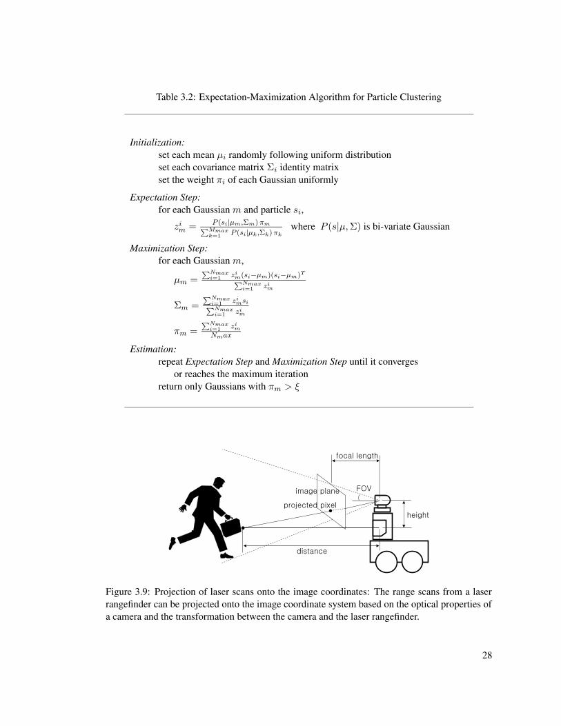
Table 3.2: Expectation-Maximization Algorithm for Particle Clustering
Initialization:set each mean µi randomly following uniform distributionset each covariance matrix Σi identity matrixset the weight πi of each Gaussian uniformly
Expectation Step:for each Gaussian m and particle si,
zim = P (si|µm,Σm) πm
PMmaxk=1
P (si|µk,Σk) πk
where P (s|µ, Σ) is bi-variate Gaussian
Maximization Step:for each Gaussian m,
µm =PNmax
i=1zim(si−µm)(si−µm)T
PNmaxi=1
zim
Σm =PNmax
i=1zimsi
PNmaxi=1
zim
πm =PNmax
i=1zim
Nmax
Estimation:repeat Expectation Step and Maximization Step until it converges
or reaches the maximum iterationreturn only Gaussians with πm > ξ
Figure 3.9: Projection of laser scans onto the image coordinates: The range scans from a laserrangefinder can be projected onto the image coordinate system based on the optical properties ofa camera and the transformation between the camera and the laser rangefinder.
28

Figure 3.10: Projected laser scans: The image pixels at the same height as the laser rangefinderhave depth information.
where the focal length of the camera is l, the horizontal and vertical field-of-view of the camera
are fh and fv, the height from the laser rangefinder to the camera is d, and the image size is
w × h. This projection model assumes a very simple camera model (a pin-hole camera) for
fast computation. As a result of the projection, the image pixels at the same height as the laser
rangefinder will have depth information as shown in Figure 3.10. For ground robots, this partial
3D information can be enough for safe navigation assuming all moving obstacles are on the the
same plane as the robot. In terms of moving object tracking, if the region of a moving objects
in an image space and those pixels are overlapped, then the distance between a robot and the
moving object can be estimated. The position in the partial 3D space [x y h]T is returned as the
final estimation result.
Initial test for the integration of the 2D motion estimates and range scans from a laser rangefinder
was promising. However, more work is required for robust estimation, eg. additional filter design
to overcome the asynchronous sensor inputs. This future work will be discussed in Section 3.7.
3.6 Experiments
3.6.1 Experimental Setup
The algorithms were implemented and tested in various outdoor environments using three dif-
ferent robot platforms: robotic helicopter, Segway RMP, and Pioneer2 AT. Each platform has
unique characteristics in terms of its ego-motion. The Robotic Helicopter (Saripalli et al., 2003)
in Figure 3.11 (a) is an autonomous flying vehicle carrying a monocular camera facing down-
ward. Once it takes off and hovers, planar movements are the main motion, and moving objects
on the ground stay at a roughly constant distance from the camera most of the time; however,
29

(a) Robotic Helicopter (b) Segway RMP (c) Pioneer2 AT
Figure 3.11: Robot platforms for experiments: Each platform has unique characteristics in termsof its ego-motion.
pitch and roll motions for a change of direction still generate complicated video sequences. Also,
high-frequency vibration of the engine adds motion-blur to camera images.
The Segway RMP in Figure 3.11 (b) is a two-wheeled, dynamically stable robot with self-
balancing capability. It works like an inverted pendulum; the wheels are driven in the direc-
tion that the upper part of the robot is falling, which means the robot body pitches whenever it
moves. Especially when the robot accelerates/decelerates, the pitch angle increases by a signif-
icant amount. Since all sensors are directly mounted on the platform, the pitch motions prevent
direct image processing. Therefore, the ego-motion compensation step should be able to cope
with not only planar movements but also pitch motions.
The Pioneer2 AT in Figure 3.11 (c) is a typical four-wheeled, statically stable robot. Since
the Pioneer2 robot is the only statically stable platform among these robot platforms, we drove
the robot on the most severe test environment. Figure 3.14 and Figure 3.17 show the rocky terrain
where the robot was driven. In addition, the moving objects were occluded occasionally because
of the trees in the environment.
The computation was performed on embedded computers (Pentium III 1GHz) on the robots.
Low resolution (320x240 pixels) input images were chosen for real-time response, and the track-
ing algorithm was able to process five frames per second. Since the algorithm is supposed to run
in parallel with other processes (eg. navigation and communication), less than 70 percent of the
CPU time was dedicated for tracking.
3.6.2 Experimental Results
The snapshots of the particle filter tracking moving objects are shown in Figure 3.12–3.14. The
maximum number of particles was set to 5,000, and the minimum number of particles was set
30

Figure 3.12: Snapshots of particle filter tracking a moving object: from Robotic helicopter
to 500. The figures show that the particle filter reduces the number of particles for efficient
estimation when it converges.
The performance of the tracking algorithm was evaluated by comparing to the positions of
manually tracked objects. For each video sequence, the rectangular region of moving objects
were marked manually and used as ground truth. Figure 3.15–3.17 shows this evaluation process.
The left windows show the input images, and the right windows show the posterior distribution
(Gaussian mixture) functions. The thick rectangles indicate the position of manually-tracked
objects, the thin rectangles indicate the output of the tracking algorithm, and the thin lines show
the distance between the center of the rectangles. The final evaluation result is shown in Table 3.3.
Motions is the number of moving objects over the total number of frames. Detected is the total
number of detected objects, and True + and False + are the number of correct detections and
the number of false-positives. Detection Rate shows the percentage of moving objects correctly
detected, and Avg. Error is the average Euclidean distance in pixels between the ground truth and
the output of tracking algorithm. The average distance error should not be considered as actual
error measurement since the tracking algorithm does not perform an explicit object segmentation;
it may track a part of an object that generates motion while the ground truth always tracks the
whole objects even though only part of the object moves.
31

Figure 3.13: Snapshots of particle filter tracking a moving object: from Segway RMP
Figure 3.14: Snapshots of particle filter tracking a moving object: from Pioneer2 AT
32

Figure 3.15: Performance evaluation: tracking from Robotic helicopter
Figure 3.16: Performance evaluation: tracking from Segway RMP
33

Figure 3.17: Performance evaluation: tracking from Pioneer2 AT
Platform Motions Detected True + False + Detection Rate Avg. ErrorRobotic helicopter 35 / 43 29 29 0 82.86 % 13.26Segway RMP 220 / 230 208 206 2 93.63 % 20.29Pioneer2 AT 172 / 195 126 114 12 66.28 % 13.54
Table 3.3: Performance of moving object detection algorithm
34

The Robotic helicopter result shows that the tracking algorithm missed six objects, but five
of them were the cases when a moving object was introduced and showed only partially on
the boundary of the image plane. Once the whole object entered into the camera field-of-view,
the tracking algorithm detected it robustly. For the Segway RMP result, the detection rate was
satisfactory, but the average distance error was larger than the others. The reason was that the
walking person was closer to the robot and the tracking algorithm often detected the upper body
only, which caused a constant distance error. The Pioneer2 AT result was the worst; however,
as explained in the previous section, the terrain for the experiment was more challenging and the
input images were more blurred and unstable.
3.7 Discussion
The individual motion tracker using a camera showed stable motion-tracking capability in 2D
image space by adopting a probabilistic filter at the end of the processing sequence. However,
the tracker sometimes generates transient position errors in 3D space when the rotational velocity
of the robot is high. The conversion from 2D to 3D using a laser rangefinder assumes perfect
synchronization between a camera and a laser rangefinder, which is unachievable in real-robot
experiments. Since there is always unknown delay between the image capture time and the range
retrieval time, laser range scans are projected at wrong places when a robot rotates at high speed.
We believe that such errors can be reduced by adding a second probabilistic filter for 3D-position
estimation, or by modifying the current probabilistic filter such that the measurement model in-
cludes not only difference images but also projected distance information. This is part of our
future research plan.
35

Chapter 4
Cooperative Multi-Target Tracking
A cooperative motion strategy for multiple target tracking system is presented in this chapter. The
single-robot tracking algorithm was described in Chapter 3; this capability is subsumed within
the multi-robot system design.
4.1 Problem Statement Revisited
When the sensors of a tracking system are mobile robots, tracking performance can be improved
by re-positioning robots in response to the motion changes of targets. As explained in Sec-
tion 2.1.6, there are two kinds of cooperations: uncertainty reduction and task allocation. The
latter type of cooperation is considered in this thesis. The precise problem statement is:
Input Estimated poses of M robots and estimated positions of n tracked targets (out
of total N targets) in a bounded environment (M � N )
Output Motion commands for M robots
Goal Maximize the number of tracked targets n over time T
Observation =
T∑
t=0
n
N×
1
T× 100 (4.1)
Constraints No prior knowledge of the number of robots or targets, and no target
motion model.
The multi-target tracking problem using a group of mobile robots can be treated as a task
allocation problem; given a group of agents (robots) and a group of tasks (targets), assign each
task to the proper agent so that the overall performance (the total number of tracked targets over
time) is maximized. However, when the number of targets N is much bigger than the number of
36

robots M , it is not preferable to compute the allocation of individual targets because of increasing
complexity of allocation algorithm. We propose a Region-based Approach as a more efficient
target allocation method; targets are grouped by the current positions, and each robot is allocated
to a group of targets.
The Region-based Approach algorithm is described conceptually in Section 4.3. In the fol-
lowing sections, the algorithm is specialized for restricted real-world environments. Section 4.4
explains how the algorithm can be implemented on a real system for unstructured environments,
and Section 4.5 suggests a coarse discretization of the algorithm for structured environments by
exploiting environmental features.
4.2 Related Work
Various distributed algorithms have been proposed for multi-robot coordination with applications
to multi-target tracking. The ALLIANCE architecture (Parker, 1999) achieves target-assignment
by the interaction of motivational behaviors. If a target was not tracked for a while, the robot
which was supposed to track the target would give up and another robot in a better position
would take up the target. In the BLE architecture (Werger and Mataric, 2000), if a particular robot
thinks it is best suited to track a specified target, it stops other robots from tracking the target by
broadcasting inhibition signals over the network. The Murdoch architecture (Gerkey and Mataric,
2001) showed that target-assignment problem can be solved using a principled publish/subscribe
messaging model; the best capable robot is assigned to each tracking task using a one-round
auction.
There have been other approaches that determine robot poses without explicit target assign-
ment, especially when the ratio of the number of robots to the number of targets is close to
1.0. In (Spletzer and Taylor, 2003), the configuration of a team of mobile robots was actively
controlled by minimizing the expected error in tracking target positions, and a reactive motion
planner was reported in (Murrieta-Cid et al., 2002) that maximizes the shortest distance that a
target needs to move in order to escape an observer’s visibility region.
The Pursuit-Evasion problem introduced in (Yamashita et al., 1997) is a formally simplified
tracking problem. The goal is to find continuously-moving intruders using a single or multiple
searchers with flashlights that emit a single ray of light. Yamashita et al. (1997) presents upper
and lower bounds of the number of necessary searchers in a given environment (a simple polygon)
and four measures of shape complexity of the environment (the number of edges, the number of
reflex vertices, the bushiness, and the size of a minimum guard set). Guibas et al. (1997) extend
37

the problem to exploit a visible area instead of a single ray of light. Several bounds on the number
of pursuers are defined and the complete algorithm for a single pursuer case is presented.
4.3 Region-based Approach
The Region-based Approach is based on the following fundamental assumption:
For two comparably sized regions, more robots should be deployed in the one with
the higher number of targets.
Instead of allocating targets to each robot, the mobile robots are allocated to each region based on
the target distribution and robot distribution. The robot density and the target density are defined
for each position in an environment, and a mobile robot is attracted to (or repulsed from) the
position based on those density estimates. For example, the less targets a region has, the less
robots the region requires, and the more robots the current region has, the more robots in that
region are free to move to other regions. Our approach assumes the following:
Global Communication The robot poses and estimated target positions are exchanged
among robots so that all robots can make decisions based on global informa-
tion. However, the decision making is still distributed based on the collected
information, which is maintained independently; the collected information can
(and does in reality) vary from robot to robot.
Global Localization All robots share a global coordinate system so that the po-
sitions of targets detected by different robots can be translated into a single
coordinates. Actual implementation of localization methods are explained in
Chapter 5 and Chapter 6
Bounded Environment The size of an environment is bounded by the communica-
tion range among robots, not by the intrinsic limitation of our algorithm.
Robust Tracker The cooperative tracking algorithm is decoupled from the low-
level target tracker; such a single-robot tracker is described in Chapter 3.
Unknown Target Model The cooperative tracking algorithm requires no prior knowl-
edge of target maneuvers.
In order to demonstrate how a robot maintain the “density estimates” or determine the most
“urgent” region in the following sections, we use the situation in Figure 4.1 as an example.
38

10 20 30 40 50 60 70 80 90 100
10
20
30
40
50
60
70
80
90
100
robottarget
Figure 4.1: Positions of mobile robots and targets in a bounded environment: Red circles indicatethe position of robots, and the blue crosses indicate the position of tracked targets.
4.3.1 Relative Density Estimates as Attributes of Space
In order to compute robot and target density values at each position, models for robot position,
target position, and region boundary are required. Based on the output of a robot localization
algorithm, the position of a robot can be modeled by a delta function or a Gaussian function.
When the localization algorithm returns an exact position (xi) as the best estimate, the robot
position is modeled using a delta function.
ri = δ(xi) (4.2)
When the localization algorithm returns a center position (µi) as the best estimate and a covari-
ance matrix (Σi) as uncertainty estimate, a bi-variate Gaussian model is adequate.
ri = N(µi, Σi) (4.3)
The robot distribution r over an environment is computed by summing the individual models.
r =∑
i
δ(xi) (4.4)
r =∑
i
N(µi, Σi) (4.5)
39

(a) Delta function model (b) Gaussian model
Figure 4.2: Robot distribution model: (a) is preferable when a robot localization method returnsa position estimate only, and (b) is adequate when it returns both a position estimate and a uncer-tainty estimate. The positions of robots are shown in Figure 4.1.
Figure 4.2 (a) shows the robot distribution using the delta function model, and Figure 4.2 (b)
shows the robot distribution using the bi-variate Gaussian model when the positions of robots are
as in Figure 4.1.
In similar way, the target distribution can be computed. Based on the output format of a
underlying target tracker, a delta function model or a bi-variate Gaussian model can be used. The
target distribution t over an environment is computed as follows:
t =∑
i
δ(xi) (4.6)
t =∑
i
N(µi, Σi) (4.7)
Figure 4.3 (a) shows the target distribution using the delta function model, and Figure 4.2 (b)
shows the target distribution using the bi-variate Gaussian model when the positions of targets
are as in Figure 4.1.
To define the density estimates, a region boundary R of a unit space must be defined. Two pos-
sible models can be used: binary model and Gaussian model. The binary model in Equation 4.8
defines a region boundary with radius r, which is conceptually simple and computationally cheap.
The shape of the boundary is shown in Figure 4.4 (a).
R(x) =
1.0 if |x| < r
0.0 otherwise(4.8)
40

(a) Delta function model (b) Gaussian model
Figure 4.3: Target distribution model: (a) is preferable when a target tracker returns position esti-mates only, and (b) is adequate when it returns both position estimates and uncertainty estimates.The positions of targets are shown in Figure 4.1.
(a) Binary region model (b) Gaussian region model
Figure 4.4: Region models for density computation: (a) is conceptually simple and computation-ally cheap, but (b) is preferable if a differentiable output is required.
41

Robot Distribution ModelDelta Function Model Bi-variate Gaussian Model
BinaryRegionModel
GaussianRegionModel
Figure 4.5: Robot density distribution: combinations of different robot distribution models anddifferent region boundary models. The positions of robots and targets are shown in Figure 4.1.
A Gaussian model can be used to define a region boundary when a differentiable output is pre-
ferred. The Gaussian distribution is zero-centered and the boundary is determined by a covariance
matrix Σ. The shape of a boundary is shown in Figure 4.4 (b).
R(x) = N(0, Σ) (4.9)
The final density distribution of robots (Dr) or targets (Dt) are computed using convolution
of the robot location and region extent:
Dr(x, y) = r ⊗ R =
∞∫
−∞
∞∫
−∞
r(τ, ρ)R(x − τ, y − ρ)dτdρ (4.10)
Dt(x, y) = t ⊗ R =
∞∫
−∞
∞∫
−∞
t(τ, ρ)R(x − τ, y − ρ)dτdρ (4.11)
Figure 4.5 and Figure 4.6 show the final density distribution examples with different robot distri-
bution models and region boundary models when the positions of robots and targets are as shown
in Figure 4.1.
42

Target Distribution ModelDelta Function Model Bi-variate Gaussian Model
BinaryRegionModel
GaussianRegionModel
Figure 4.6: Target density distribution: combinations of different target distribution models anddifferent region boundary models.
4.3.2 Urgency Distribution and Utility
Given the distribution of robots Dr and the distribution of targets Dt in a bounded environment,
we define the urgency distribution u:
u(x, y) =Dt(x, y)
Dr(x, y)(4.12)
Figure 4.7 shows the urgency distribution calculated using different models. As shown in Fig-
ure 4.1, there are three groups of targets: six targets around at the coordinate (30, 30), two targets
around at (80, 80), and a single target at (75, 35). The first two groups are being observed by
robots, and those regions have relatively low urgency values as shown in Figure 4.7. However,
the last group is not being tracked with any robot, so the urgency value of the region is very high,
which means the region requires a robot.
A cost function cr for each robot can be combined to compute the final utility function for
robot control instead of simply using the urgency distribution as an utility function. For example,
the cost of motion can be integrated by multiplying a function which is inverse-proportional to
a travel distance. Figure 4.8 shows an example of those functions; the inverse cost function for
the robot at (20, 80) has a peak at the current position of the robot since the cost of traverse is
43

Robot & Target Distribution ModelDelta Function Model Bi-variate Gaussian Model
BinaryRegionModel
GaussianRegionModel
Figure 4.7: Urgency distribution: The urgency values indicate how “urgently” a region shouldbe observed based on robot and target distributions over an environment.
zero, and it decreases as it moves further from the current position because the cost of traverse
increases. The final utility distribution function is defined as:
U(x, y) = u(x, y) ×1
cr(x, y)(4.13)
It is worth noting that each robot would have a different utility distribution because of the cost
function term cr. Since the urgency distribution u is calculated using the position information of
robots and targets, every robot would maintain the same u distribution unless there is failure in
communication. However, the different positions of robots cause different costs for a region, and
eventually diverse behaviors for robots are generated.
The final utility distribution for the robot at the coordinate (20, 80) is shown in Figure 4.9.
Intuitively, the region at the coordinate (75, 35) would attract the robot since it has the highest
utility value.
4.3.3 Distributed Motion Strategy
Given the utility distribution, we define two motion strategies. If only local planning is desired,
then one possible motor command is a gradient descent method on the utility function as follows:
44
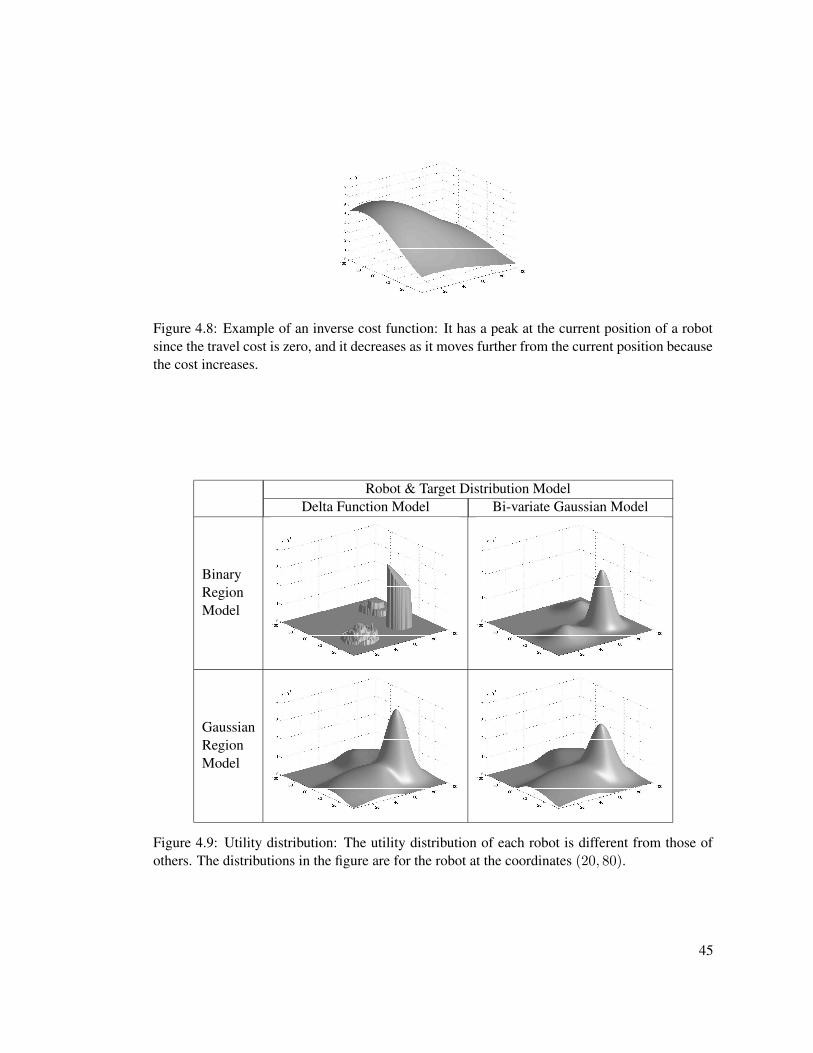
Figure 4.8: Example of an inverse cost function: It has a peak at the current position of a robotsince the travel cost is zero, and it decreases as it moves further from the current position becausethe cost increases.
Robot & Target Distribution ModelDelta Function Model Bi-variate Gaussian Model
BinaryRegionModel
GaussianRegionModel
Figure 4.9: Utility distribution: The utility distribution of each robot is different from those ofothers. The distributions in the figure are for the robot at the coordinates (20, 80).
45

x = −∇U (4.14)
If global planning is preferred, then the peak position of the utility distribution can be a goal
position:
x′ = arg max
x
U(x) (4.15)
Each robot plans its motion and executes it independently in a distributed manner, and there
is no explicit negotiation between robots. However, by sharing the position information of robots
and targets, these motion plans are coupled.
4.4 Grid Region-Based Approach
The concept of the Region-based Approach was described through an example in Section 4.3.
However, such conceptual models are not directly applicable to real-world systems because of
limited sensor range for target tracking, insufficient computing power for utility distribution eval-
uation over the environment, etc.
A fine discretization of the Region-based Approach is presented in this section, which can
be implemented for cooperative tracking in unstructured environments. A grid-based represen-
tation is used for the density estimates and the utility distribution, and the region boundaries are
determined according to the properties of an underlying target tracker.
4.4.1 Virtual Region Representation and Density Estimates
In order to compute the utility distribution for multi-robot cooperation, the robot density and
the target density should be defined first, which subsequently requires the definition of a region
boundary. For simplicity, the delta function models in Equation 4.4 and Equation 4.6 are assumed
for robot and target distributions, and the binary region model in Equation 4.8 is used for a region
boundary.
A virtual region is represented by four parameters: a center position (x, y), a radius lr for
robot density estimation, and a radius lt for target density estimation. As shown in Figure 4.10,
the radius lr and lt are determined according to the sensor range and the field-of-view of a target
tracker. For the robot density distribution, a region boundary is defined as follows:
46

Figure 4.10: Parameterized virtual region: The radius lr and lt are determined according to theproperties of a tracking sensor.
Rr(x) =
1.0 if |x − xc| < lr
0.0 otherwise(4.16)
where xc is the center of a region. In a similar way, a region boundary for the target density
distribution is defined as follows:
Rt(x) =
1.0 if |x − xc| < lt
0.0 otherwise(4.17)
Two density estimates are computed simply as follows:
Dr(x, y) = r ⊗ Rr(x, y) = the number of robots within a distance lr
Dt(x, y) = t ⊗ Rt(x, y) = the number of targets within a distance lt(4.18)
Each robot broadcasts its current position and the tracked targets’ positions, and maintains
internal estimates of Dr(x, y) and Dt(x, y) based on the broadcast packets it receives and its own
sensor readings. Due to packet loss the estimates may not accurately measure the actual values.
Further, the target density values will necessarily be inaccurate because the robots can only count
tracked targets. Lastly, both sets of estimates can (and do) vary from robot to robot.
4.4.2 Estimation of the Utility Distribution
Similar to the general Region-based Approach, the utility value for every virtual region is defined
as in Equation 4.19, where d is the Euclidean distance between the current robot position and the
center of a virtual region (x, y).
47

U(x, y)=
Dt(x,y)Dr(x,y) × icr(d) if Dr 6= 0
Dt(x, y) × α × icr(d) if Dr = 0 & Dt 6= 0
1.0 if Dr = Dt = 0
icr(d)= e− 1
2×
“
dθd
”
2
(4.19)
The utility computation is not different from the generic version in Equation 4.13 except that
it treats the mathematical exceptions (eg. infinity and zero divided by zero) separately. The
parameter α is a constant to scale the utility value in the case of infinity to a reasonably big value,
and the parameter θd is a constant to determine the inclination of the inverse cost function icr.
There are two implementation issues: (a) how to cope with the unbounded state space, and (b)
how to represent the continuous utility distribution U(x, y) efficiently. When an environment is
unbounded, then the utility distribution U(x, y) is supposed to be evaluated over the entire space
theoretically. However, the effective search space can be limited by the fact that the evaluation
is performed based on the detected targets only. In other words, the value of U(x, y) will be a
constant when the distance from the position (x, y) to the position of any robot in the system is
bigger than a certain threshold, which is θs = le + lt when le is the effective range of a tracker.
Therefore, the size of the effective search space is proportional to the number of robots in the
system.
There are two popular methods to represent a continuous function: grid method and non-
uniform (adaptive) sampling. The non-uniform sampling is beneficial when the search space is
big and the distribution of function values are concentrated on several areas (eg. the entropy of
the function is small). For the proposed target-tracking system, the search space is relatively
small, and targets can move in and out of the search space quite often. Therefore, a grid method
is adopted for the utility distribution representation.
Figure 4.11 shows a snapshot of the utility distribution. Robots are marked with empty circles,
and targets are drawn as filled circles. The color of each grid cell represents the utility value; the
darker the color is, the higher the utility value is.
4.4.3 Motion Strategy for Cooperative Target Tracking
The motion of each robot is determined in similar way to the original Region-based Approach.
The utility distribution is updated based on the latest density estimates, and Equation 4.15 is
evaluated to search the most urgent region. By changing the parameter θd of the cost function
48

Figure 4.11: Snapshot of the utility distribution: The darker the color of a grid cell is, the higherthe utility value of the region is. It is noticed that only the effective search space is evaluated.
icr(d), the chance for a robot to select a closer region with smaller utility over a farther region
with bigger utility can be controlled.
Even though the utility distribution is evaluated for limited space only, the amount of compu-
tation is still intensive because of the high update rate. The motion of each robot can be computed
more efficiently by adding an availability checking step. Before updating the utility distribution,
each robot checks if it is available to migrate to a more urgent region by evaluating Equation 4.20,
where T (x, y, lt) is the number of targets tracked by the robot in the region Rt(x, y). By checking
the availability of a robot in advance, the robot need not evaluate the utility distribution at every
cycle, which reduces the computing time.
max∀x,y
[
Dt(x, y)
Dr(x, y)× T (x, y, lt)
]
< θt (4.20)
Equation 4.20 was constructed based on the following facts:
• The less targets a region has, the less robots the region requires.
• The more robots a region has, the more robots in that region are free to move to other
regions.
• The fewer targets a robot is tracking at a given moment, the less the robot is required to
stay in its current region.
θt is a parameter that decides how easily a robot would give up tracking the current targets and
travel to other regions hoping to find a new, bigger group of targets.
49

Figure 4.12: Example of a topological map: The environment (on the left) consists of two officesand two long corridors, and the topological map (on the right) can be constructed as a graph.
4.5 Topological Region-based Approach
The Region-based Approach can be simplified further by exploiting environmental features. For
structured environments (eg. office-type indoor environment), the following assumption can be
made:
The environment can be divided into topologically simple convex regions using cer-
tain landmarks as demarcaters. Each region is assumed to be simply connected1.
Figure 4.12 shows an example of a topological map shown as a graph. In the topo-
logical map, a node corresponds to a region, and a link corresponds to a landmark.
For example, the link between two corridor regions may be a corner.
For the Topological Region-based Approach, the density estimates and the utility distribution are
maintained for nodes on a topological map, which are discrete and sparse. The advantage of this
coarse discretization is that the computation for those distribution is very cheap.
Many on-line, topological mapping techniques have been demonstrated in (Choset and Bur-
dick, 1995a,b; Dedeoglu et al., 1999; Dedeoglu and Sukhatme, 2000; Kuipers and Byun, 1991;
Kunz et al., 1999; Nagatani and Choset, 1999; Rekleitis et al., 2001; Tomatis et al., 2001), which
segment the environment into regions automatically. In this thesis, we focus on the high-level
cooperative tracking problem assuming a topological map of the environment is given a priori.
4.5.1 Density Estimates on a Topological Map
Given a topological map, every robot independently maintains two density estimates for each
node (region). The density estimates are somewhat different from Equation 4.10 & 4.11 or
1Two regions are connected with a single edge only when they are physically connected such that a robot cantraverse from a region to another.
50
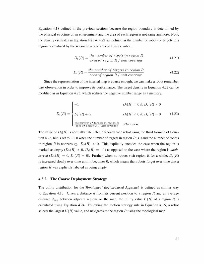
Equation 4.18 defined in the previous sections because the region boundary is determined by
the physical structure of an environment and the area of each region is not same anymore. Now,
the density estimates in Equation 4.21 & 4.22 are defined as the number of robots or targets in a
region normalized by the sensor coverage area of a single robot.
Dr(R) =the number of robots in region R
area of region R / unit coverage(4.21)
Dt(R) =the number of targets in region R
area of region R / unit coverage(4.22)
Since the representation of the internal map is coarse enough, we can make a robot remember
past observation in order to improve its performance. The target density in Equation 4.22 can be
modified as in Equation 4.23, which utilizes the negative number range as a memory.
Dt(R) =
−1 Dt(R) = 0 & Dr(R) 6= 0
Dt(R) + α Dt(R) < 0 & Dr(R) = 0
the number of targets in region Rarea of region R / unit coverage otherwise
(4.23)
The value of Dt(R) is normally calculated on-board each robot using the third formula of Equa-
tion 4.23, but is set to −1.0 when the number of targets in region R is 0 and the number of robots
in region R is nonzero eg. Dr(R) > 0. This explicitly encodes the case when the region is
marked as empty (Dr(R) > 0, Dt(R) = −1) as opposed to the case where the region is unob-
served (Dr(R) = 0, Dt(R) = 0). Further, when no robots visit region R for a while, Dt(R)
is increased slowly over time until it becomes 0, which means that robots forget over time that a
region R was explicitly labeled as being empty.
4.5.2 The Coarse Deployment Strategy
The utility distribution for the Topological Region-based Approach is defined as similar way
to Equation 4.13. Given a distance d from its current position to a region R and an average
distance davg between adjacent regions on the map, the utility value U(R) of a region R is
calculated using Equation 4.24. Following the motion strategy rule in Equation 4.15, a robot
selects the largest U(R) value, and navigates to the region R using the topological map.
51

U(R) = u(
Dt(R), Dr(R))
×davg
d
u(Dr, Dt) =
Dt
DrDr 6= 0
Dt × α Dr = 0 & Dt 6= 0
1.0 Dr = Dt = 0
α = area of region Runit coverage × θd
(4.24)
Equation 4.24 is a formalization of the following ideas:
If there is a region that has targets but does not have a robot, or if there is a region that
has more targets than robots, then some robot should move to the region. Otherwise,
a robot should move to an unobserved region (Dr = Dt = 0) for exploration. θd is a
parameter that controls how far a robot is willing to travel; for example, by setting θd
to a small number, a robot is more likely to choose a closer region with less targets
over a farther region with more targets, and vice versa.
As explained in Section 4.4.3, the computing time of the utility distribution can be saved by
adding the availability checking step. Before updating the utility values of all regions, a robot
checks if it is available to migrate to a region which more urgently needs robots. When a robot
is tracking T targets in the current region Rc, the robot is said to be available if the inequality in
Equation 4.25 is satisfied.
Dt(Rc)
Dr(Rc)× T < θt (4.25)
Equation 4.25 was constructed based on the same idea described in Section 4.4.3. θt is a param-
eter that decides how easily a robot would give up tracking the current targets and travel to other
regions hoping to find a new, bigger group of targets.
4.5.3 Target Tracking within a Region
The Topological Region-based Approach requires one more motion strategy: movements within
a region since a region corresponds an space, not a position. Each robot tries to maximize the
number of tracked targets within a region. In order to track multiple targets using a camera with
limited field of view (FOV), a robot should be positioned close enough not to lose any target,
and far enough to keep all targets within its FOV. In order to approach this position, each robot
calculates the center of gravity (COG) of the current tracked targets as shown in Figure 4.13. The
52

COG
FOV
Target
Target
Target
Target
Robot
Figure 4.13: Following targets within a region: A robot maintains a proper distance from thecenter of gravity (COG) of the current tracked targets.
robot attempts to keep at a distance (Equation 4.26) from the COG where dmax is the distance
between the COG and the target furthest from the COG in the group.
distance =dmax
sin(FOV/2)(4.26)
4.6 Discussion
Two different levels of simplification of the Region-based Approach are presented for the coop-
erative target tracking using a group of mobile robots. The Grid Region-based Approach adopts
a grid representation for the utility distribution. This method is efficient in the sense that the best
region boundary is selected according to the tracker properties and targets are grouped automat-
ically. On the other hand, the Topological Region-based Approach exploits a topological map of
an environment, which provides pre-partitioned regions. Since the representation is discrete and
sparse, the required computing power is very low. However, this method is valid only for struc-
tured environments, and an additional motion strategy (movement within a region) is required.
The performance of those two methods is analyzed in the following chapters.
53

Chapter 5
Experiments in Structured Environments
The problem of tracking multiple anonymous targets in a structured, planar environment using
a network of communicating robots and optionally stationary sensors. The Topological Region-
based Approach described in Section 4.5 is exploited for cooperation among multiple robots. For
the performance analysis, three experiments are performed:
1. The Topological Region-based Approach is compared to a ‘naive’ local-following strategy
in three different environments with varying degree of occlusion.
2. The environment is held constant, and two techniques (robot density and visibility) for
computing urgency distributions were compared.
3. Different combinations of mobile robots and stationary sensors were compared in a given
environment.
5.1 System Design and Implementation
Figure 5.1 shows a behavior-based control architecture for the mobile robots, which implements
the Topological Region-based Approach. The controller consists of three layers: Motor Actuation
Layer, Target Tracking Layer, and a Monitoring Layer.
5.1.1 The Motor Actuation Layer
The Motor Actuation Layer controls robot deployment; for example, it causes a robot to approach
targets, or traverse from one region to another. There are four modules in this layer.
The RobotMove module is a repository of basis behaviors (Mataric, 1997), and always per-
forms one of these behaviors as selected by the RobotDispersion module. The basis behaviors
are RandomWandering, WallFollowing, TargetFollowing, SpotApproaching, and TurningAround.
54

Figure 5.1: Behavior-based robot control architecture: Behaviors are drawn as rectangles, andsensors are shown as half ellipses (read only) or full ellipses (read/write). Thin arrows indicateinformation flow (a module can share its internal data with other modules), and thick arrowsindicate parameter modification (one module can change other modules’ behavior). Dashed linesshow user-selected debugging information, and double lines emphasize that a behavior generatesdecoupled motor control commands (one for speed control and one for heading control).
Other than TargetFollowing which needs some explanation, the others are relatively standard and
self-explanatory. TargetFollowing acts differently when a robot uses the robot density (Equa-
tion 4.21) for computing the urgency distribution and when it uses the visibility (Equation B.1).
In the former case, TargetFollowing causes a robot to approach the center of gravity (COG) of all
tracked targets (Figure 4.13). It also controls the distance between the robot and the COG based
on how much the targets are spread. However, in the latter case, TargetFollowing makes a robot
approach the COG of only selected targets and keep away from other robots (Figure B.2).
The RobotDispersion module disperses robots to regions. It checks a robot’s availability by
accessing the internal map (Map), and drives the robot to the most urgent region by following a
path generated by Map module.
The MotorControl module generates actual motor control signals (Speed & Turnrate) based
on input signals from other modules. It has four different modes: Sum, Min, Max, and One.
All inputs are integrated in Sum mode, or a single, specified input is used in One mode; mini-
mum/maximum inputs are selected in Min/Max mode.
The ObstacleAvoidance module is for safe navigation. It acts differently when a robot is
tracking targets and when it is not. It executes only speed control when a robot is tracking
55

targets, and leaves turnrate control to RobotMove (more specifically TargetFollowing). However,
it regulates both speed and turnrate control when a robot is not tracking a target.
5.1.2 The Target Tracking Layer
The modules in the Target Tracking Layer detect targets, estimate their positions, and interchange
this information among robots so that each robot can compute the density estimates defined ear-
lier.
The RobotLocalization module keeps track of a robot’s position. Since a robot calculates the
positions of tracked targets based on its local coordinate system, knowing the robot’s position
is important for accurate target position estimation. This module estimates the robot’s position
based on odometry all the time, and compensates drift error whenever it sees laser beacons1 which
are disseminated in the environment at region boundaries. Given the global positions of the laser
beacons and distance/bearing information to them, the RobotLocalization module can estimate
the position and heading of a robot very accurately, and can correct odometry error.
The ColorBlobTracker module detects targets of certain colors, and calculates their positions.
It uses a camera to detect targets and to calculate bearing to them, and uses a laser rangefinder
to measure the distance to the targets. More details about the tracker can be found in (Jung
and Sukhatme, 2001). The positions of targets in the robot’s local coordinates are saved for the
TargetFollowing behavior, and the positions in global coordinates are broadcast over the wireless
network at the speed of 10 Hz.
The MapUpdate module receives the broadcast packets, and updates density information in
the Map module. Each target is identified by its global position; if the distance between two target
positions is smaller than the twice length of a robot body, the two targets are assumed as a single
target. The Map module is a passive data storage; all its contents are updated by the MapUpdate
module. However, it has a functionality of a path planner; it can generate topological paths from
one region to a specified goal region when there is a request from other modules.
5.1.3 Monitoring Layer
The Monitoring Layer is not directly related to the controller, but it provides a convenient means
to observe the internal status of the controller during operation. Since the bandwidth of the
wireless network is limited, each robot sends its internal information only when there is a request
1The laser beacon (Howard et al., 2001) is a simple bar-code constructed using strips of retro-reflective paper.Based on the reading from a SICK laser rangefinder, a robot can compute the ID, range, bearing, and orientation foreach visible beacon.
56

(a) Robot (b) Target
Figure 5.2: Configurations for robots and targets: Pioneer robot is equipped with a SICK laserrangefinder and a Sony PTZ camera, and each target was a Pioneer robot carrying a bright-coloredcylinder
from an external monitoring program. Currently, this layer is used for debugging only, but it can
be used for inter-robot communication for future extension.
The MonitorServer module is a thread-based server program; it always listens to a specified
port, and sends selected internal data of other modules when there is a request. The module can
serve more than one client at a time.
5.2 Experimental Setup
To evaluate our approach, we performed experiments with ActivMedia Pioneer DX-2 robots and
the Player/Stage software platform. Pioneer robots equipped with a SICK laser rangefinder and a
Sony PTZ camera were used for tracking, and each target was a Pioneer robot carrying a bright-
colored cylinder (see Figure 5.2).
Tracking performance was evaluated using Equation 5.1. Following (Parker, 1997) we define
the Observation as
Observation =T
∑
t=0
n
N×
1
T× 100 (5.1)
where N is the total number of targets, n is the number of targets being tracked at time t and the
experiment runs over time T .
57

Figure 5.3: System architecture for targets: A target shows four different behaviors (wander,follow walls, turn in place, or stop) in random combination.
5.2.1 Target Modeling
Pioneer robots were used as moving targets. Each target robot uses sonar sensors for obstacle
avoidance, and carries a bright-colored cylinder that is easily detected by a vision system. As
shown in Figure 5.3, targets have four different behaviors: Random-Wandering, Wall-Following,
Random-Turning, and No-Move. Each behavior is chosen randomly with probabilities (0.3, 0.3,
0.2, 0.2) in order. This target model showed sufficiently unpredictable, complex movement during
experiments.
5.2.2 Environment Complexity
After having observed several simulations, we realized that the characteristics of the environment
affect the system performance. The shape of the environment, in particular how obstructed it is,
seems to be significant. In order to investigate this correlation between the Topological Region-
based Approach and characteristics of environment, we chose three distinct environments shown
in Figure 5.4. The first environment, Corridors, consists of long, narrow regions which cause
many occlusions. Each region is narrow enough that a single target may cause serious occlusion to
the trackers. The second environment, Concave, consists of several relatively big regions with few
occlusions. The last environment, Convex, is a single empty space which has no occlusion at all.
Occlusions can be caused only by targets or other robots. The areas of these three environments
are equal.
A formal approach to analyze the complexity of environment models has been introduced in
(Cazals and Sbert, 1997). The basic idea of the approach is to generate uniformly distributed
random rays, and to compute statistics such as how often rays intersect with models, how long
truncated segments are, etc. Various characteristics about 3D models can be inferred from these
58

(a) Corridors (b) Concave (c) Convex
Figure 5.4: The simulation environments: The black regions are occupied and the rest is freespace. The associated topological maps are shown as graphs. (a) Corridors consists of long,narrow regions which cause many occlusions. (b) Concave consists of several relatively bigregions with few occlusions. (c) Convex is a single empty space which has no occlusion at all.
statistics. We utilize this approach in order to measure the complexities of our planar environ-
ments.
As explained in (Cazals and Sbert, 1997), two end-points of rays must be selected from the
circumcircle of environment images for uniform distribution, not from the bounding box. In order
to meet this restriction, two angles (θ1, θ2) were randomly generated, and the two end-points
(x1, y1) and (x2, y2) were computed as follows when r is the radius of the circumcircle:
x1 = r × cos(θ1), y1 = r × sin(θ1)
x2 = r × cos(θ2), y2 = r × sin(θ2)
If a ray did not intersect with the bounding box of environment images at all, the ray did not
count.
Table 5.1 shows the statistics of the three environments. The environments with several tar-
gets present were also tested in order to investigate how the complexities change when there are
robots/targets in the environments. The targets were evenly distributed in regions. In Table 5.1,
p0 is the probability that a ray does not intersect with any objects, eg. walls, robots, and targets.
enGint is the average of the number of intersection points, and σenG
int is its standard deviation.
µCL is the average of the length of free lines2, and σCL is its standard deviation. Especially, p0
2Free lines are the segments of rays that divided by intersection points. The lengths of the free lines are normalizedwith the longest free line.
59

Environment # targets # rays p0 enGint σenG
int µCL σCLCorridors 0 10,000 0.3003 1.9552 1.5201 0.2714 0.2438Corridors 2 10,000 0.2963 2.0394 1.6076 0.2657 0.2445Corridors 4 10,000 0.2901 2.1212 1.6646 0.2596 0.2422Corridors 6 10,000 0.2876 2.1998 1.7273 0.2555 0.2432Corridors 8 10,000 0.2849 2.2784 1.8201 0.2509 0.2413Concave 0 10,000 0.7600 0.4800 0.8542 0.4678 0.2798Concave 2 10,000 0.7260 0.5738 0.9600 0.4478 0.2826Concave 4 10,000 0.6784 0.7140 1.0983 0.4265 0.2852Concave 6 10,000 0.6331 0.8188 1.1447 0.4131 0.2853Concave 8 10,000 0.6015 0.9082 1.1995 0.3992 0.2829Convex 0 10,000 1.0000 0.0000 0.0000 0.5639 0.2462Convex 2 10,000 0.9406 0.1196 0.4776 0.5301 0.2601Convex 4 10,000 0.8800 0.2510 0.6950 0.5057 0.2687Convex 6 10,000 0.8338 0.3678 0.8613 0.4785 0.2724Convex 8 10,000 0.8003 0.4688 0.9985 0.4594 0.2730
Table 5.1: Complexity of the environments as a function of number of targets: Only targets areincluded for the complexity analysis because robots are part of the tracking system, not part of theenvironment. However, since a robot has the same size with a target, the result can be interpretedsuch as the number of targets indicates the number of objects including robots.
is a nice indicator showing how much occlusion an environment has, and µCL can be an indicator
showing how big (wide) each region is.
As expected, Corridors showed small p0 and µCL, which means it has significant occlusion
and its regions are narrow. On the other hand, p0 of Convex was big since it has little occlusion.
The µCL values of both Concave and Convex were big because their regions are wide. Needless
to mention, the more targets, the higher complexity.
5.2.3 Experiment Design
Three experiments were performed with various configurations. Two of them were performed
using the Stage simulator, and the third experiment was performed using Pioneer DX-2 robots.
5.2.3.1 Region-based versus Local-following Strategy
The Topological Region-based Strategy was compared with a Local-following Strategy. The
Topological Region-based Strategy uses the system described in Section 6.1, and the Local-
following Strategy uses the same architecture without the RobotDispersion module. The Local-
following Strategy still tries to maximize the number of tracked targets in the current region by
60

maintaining a proper distance from a group of targets as explained in Figure 4.13. The best sce-
nario for the Local-following Strategy would be that many targets gather in an open space and
stay in a large, circle-shaped group; a single robot would be able to keep track of most of the
targets in the group. The worst scenario for the Local-following Strategy would be that all robots
track the same single target and the rest of targets stay away from the target being tracked; since
robots never give up the current tracked target, they would never leave the current region to move
to other regions which contain other targets. On the other hand, the Region-based Strategy causes
a robot to relinquish tracking the current tracked target to explore other regions when there are
more than enough robots in the current region; therefore, the worst scenario would never hap-
pen. The purpose of this comparison is to measure if the map-based coarse control causes an
improvement in tracking performance.
5.2.3.2 Robot Density versus Visibility
Two variants of the Topological Region-based Approach are compared. With the Robot Density, a
robot tracks all targets in its sensing range. However, when robots get too close to each other, the
overall performance might reduce. On the other hand, with Visibility described in Appendix B, a
robot covers a wider area within a region by keeping away from other robots, but this may result
in the loss of some targets in the process of receding.
In order to perform experiments with various configurations and minimize the effect of un-
necessary factors, the Stage simulator is used with the Corridors environment shown in Figure 5.4
(a). Thus this experiment does not vary the environment.
5.2.3.3 Mobile Robots versus Embedded Sensors
Another interesting issue in multi-target tracking using multiple sensors is whether adding a mo-
bile sensor (eg. a mobile robot) is always more helpful to improve tracking performance com-
pared to adding a stationary environment-embedded sensor (eg. a security camera). Each sensor
has its own advantages. For example, a mobile sensor can cover wider area over time, and can
adapt to targets’ movement patterns. On the other hand, a fixed sensor can be installed at the best
position depending on the environments, and it causes less interference.3
Since we wanted a realistic environment for this test, the experiments were performed using
real robots on the second floor of our Computer Science Building. Figure 5.5 shows the map of
the floor and its topological map; it consists of two offices and two long corridors. The figure also
3Actual cost of mobile robots and fixed sensors is not considered for this comparison since we only focus on theperformance of cooperative tracking strategies using heterogeneous sensors.
61

Figure 5.5: Environment for real-robot experiments: It consists of two offices and two longcorridors. The laser beacons are shown as dark gray, thick lines on the walls, and the position ofstationary sensors are marked by ⊗ symbols.
shows the positions of the laser beacons (dark gray, thick lines) and stationary sensors (⊗ marks).
In this study the environment and control strategy were held constant and the ratio of the mobile
to stationary trackers was varied.
5.3 Experimental Results
5.3.1 Region-based versus Local-following Strategy
The simulations were performed with various configurations in three different environments. We
fixed the number of robots at 2, and changed the number of targets from 4 to 20 in steps of 2.
Each configuration ran for 10 minutes a total of 9 times, and the average performance was taken
as the final result. The experimental results are shown in Figure 5.6.
5.3.2 Robot Density versus Visibility
The simulations were performed with various configurations using the Corridors environment.
We fixed the number of robots at 2, and changed the number of targets from 4 to 20 in steps of 2.
Each configuration ran for 10 minutes a total of 9 times, and the average performance was taken
as the final result. The result is shown in Figure 5.7.
5.3.3 Mobile Robots versus Embedded Sensors
We fixed the number of targets at 4, and used a total of 2 sensors in three different combinations:
with only two stationary sensors, with one stationary sensor and one mobile robot, and with two
mobile robots. Each configuration was tested over 3 trials, and each trial ran for 10 minutes.
The average performance is shown in Figure 5.8. When the robots were used, we performed the
experiment twice, using both the Region-based Strategy and the Local-following Strategy.
62

0
5
10
15
20
25
30
35
40
45
50
5 10 15 20
Obs
erva
tion
(%)
Number of Targets
Region-basedLocal-following
(a) Corridors
35
40
45
50
55
60
65
70
75
5 10 15 20
Obs
erva
tion
(%)
Number of Targets
Region-basedLocal-following
(b) Concave
30
35
40
45
50
55
60
65
70
75
80
5 10 15 20
Obs
erva
tion
(%)
Number of Targets
Region-basedLocal-following
(c) Convex
Figure 5.6: Simulation results comparing the performance of the two strategies: The number ofrobots was fixed at 2, and the number of targets varied from 4 to 20 in steps of 2.
63
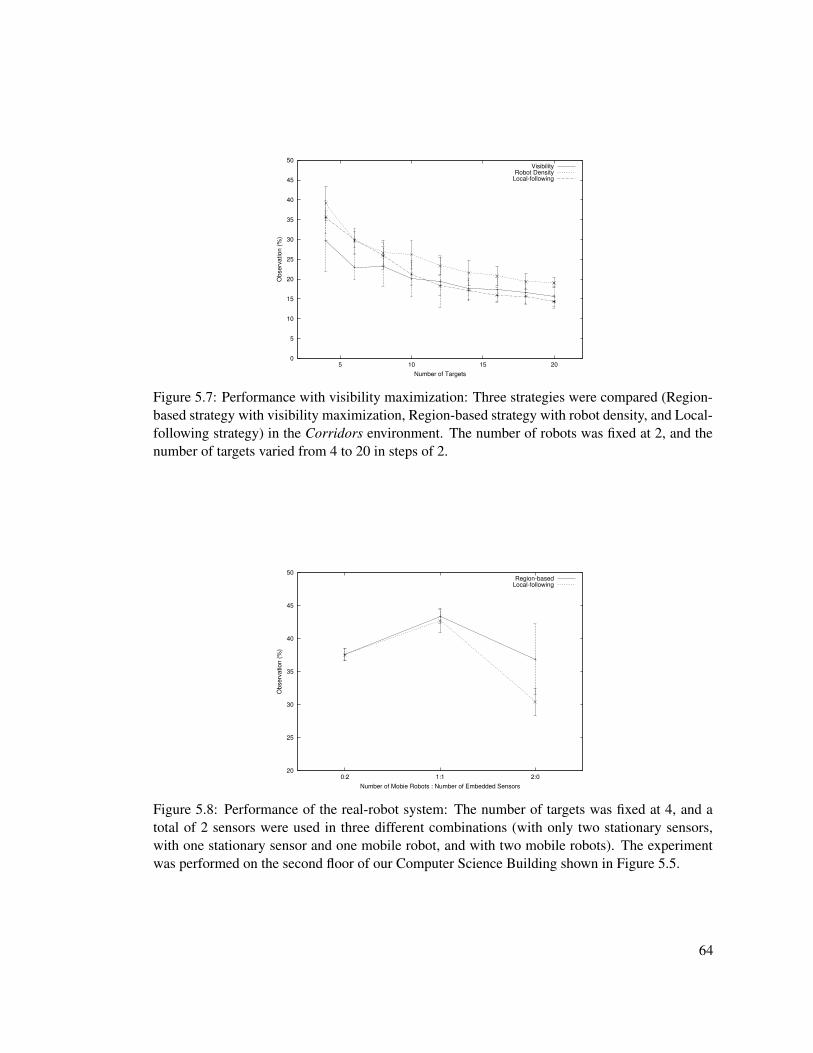
0
5
10
15
20
25
30
35
40
45
50
5 10 15 20
Obs
erva
tion
(%)
Number of Targets
VisibilityRobot Density
Local-following
Figure 5.7: Performance with visibility maximization: Three strategies were compared (Region-based strategy with visibility maximization, Region-based strategy with robot density, and Local-following strategy) in the Corridors environment. The number of robots was fixed at 2, and thenumber of targets varied from 4 to 20 in steps of 2.
20
25
30
35
40
45
50
0:2 1:1 2:0
Obs
erva
tion
(%)
Number of Mobie Robots : Number of Embedded Sensors
Region-basedLocal-following
Figure 5.8: Performance of the real-robot system: The number of targets was fixed at 4, and atotal of 2 sensors were used in three different combinations (with only two stationary sensors,with one stationary sensor and one mobile robot, and with two mobile robots). The experimentwas performed on the second floor of our Computer Science Building shown in Figure 5.5.
64
# targets Corridors Concave Convex4 0.112957 0.022510 0.0001176 0.808498 0.334473 0.0001208 0.660541 0.369265 0.06259710 0.007183 0.638818 0.04662112 0.000549 0.378994 0.00336714 0.006264 0.608437 0.00012416 0.000445 0.786089 0.00004218 0.001258 0.184465 0.00005920 0.000008 0.062607 0.000093
Table 5.2: Significance values from T-test as a function of number of targets and environmentcharacteristic
5.4 Discussion
5.4.1 Region-based versus Local-following Strategy
In the Corridors environment, the Region-based Strategy showed better performance, especially
when the number of targets was large. Since the regions are narrow and many occlusions are
caused, it is almost impossible for a single robot to track more than two targets at a time, which
means cooperation among robots is indispensable. On the other hand, the performance of the
Region-based Strategy, in the Convex environment, was not as good as that of Local-following
Strategy. This can be explained by the fact that a robot is able to track targets in other regions
without traversing to those regions in the empty environment because there is zero occlusion. This
benefit is maximized for the Local-following Strategy, but not for the Region-based Strategy. Both
strategies showed almost the same performance in Concave, whose shape causes a small amount
of occlusion.
We performed a t-test with each data points pair in order to see if the results from the two
strategies show significant difference statistically. Table 5.2 shows the significance values of the
t-test; a small number implies that the two distributions are statistically different. As expected,
the significance values of Concave were big, and those of Corridors and Convex were small.
The simulation results show a strong correlation between robot coordination strategies and
environment shape. The data in Figure 5.6 suggest that in environments with a low value of
p0, the Topological Region-based Approach out performs the Local-following Strategy, and in
environments with a high value of p0, the reverse is true. However, there are unobserved factors
which might be critical to the overall performance, eg. region decomposition. The Topological
Region-based Approach may perform differently when an environment is decomposed into few
big regions and when the same environment is divided into many fine regions. Also, the region
65

# targets vs Robot Density vs Local-following4 0.007200 0.0678676 0.000737 0.0000778 0.114616 0.21745710 0.008551 0.55193312 0.117852 0.67629014 0.013156 0.74372916 0.020076 0.30030518 0.049254 0.43339220 0.003620 0.223343
Table 5.3: Significance values from T-test as a function of number of targets and different strate-gies
decomposition method may have to be varied depending on environment shape; for instance,
region size should be small when the complexity of an environment is high, and vice versa. We
plan to investigate these issues in future work.
5.4.2 Robot Density versus Visibility
As shown in the t-test result (Table 5.3), the Topological Region-based Approach using the Visibil-
ity did not show significant difference from the Local-following Strategy. There are two possible
explanations for this.
First, the coverage estimation method might have been inappropriate. Because of lack of
global, geometrical information and real-time requirement, simple approximation methods were
utilized as much as possible. For example, each sensor’s coverage was computed by integrating
real laser readings, but a single simplified sector was used for overlap computation. Also, small
error was ignored. For instance, overlap was computed for all possible pairs of robots within a
region; when the coverage of three robots (A, B, and C) are overlapped, the coverage intersection
A∩B∩C is subtracted once more unnecessarily and never compensated.
Second, the visibility maximization method described in Appendix B assumes that tracking
sensor is omni-directional, which is not valid in both simulation and real robots. In the current
visibility maximization method, when a robot detects other robots, it abandons tracking targets
which are positioned closer to the other robots. By doing this, robots can keep distance from each
other without explicit communication. In Figure B.2 (c) this method works properly since the
upper robot is facing down. However, if the upper robot were facing up, the lower robot would
still move same and the other two targets would not be tracked anymore. This problem is caused
because the current tracking sensor cannot detect other robots’ heading.
66

It is expected that better implementation of visibility maximization method would improve
its overall performance.
5.4.3 Mobile Robots versus Embedded Sensors
The general tracking performance in the real-robot experiments was not as good as that in the
simulation. There are several explanations. First, the effective range of the real vision system
(around 4.5m) was much shorter than the range of the simulated one (8m). Also, the field of view
(FOV) of the real camera (90 degrees) was not as wide as the FOV of the virtual camera (120
degrees). Second, the environment for the real-robot experiments was much more complex; for
example, the connection between offices and corridors (doors) was narrow enough to cause the
robots difficulties. Lastly, the odometry error of the real robot was larger, and caused unfavorable
effects on navigation; for example, it took longer to traverse from a region to another region.
In case of using two stationary sensors, the performance depends on targets’ movement. As
shown in Figure 5.8, the standard deviation was small (±2%), which signals that the targets spread
out evenly over the environment. When a mobile robot was used together with an embedded
sensor, the overall performance was higher than any other cases. As shown in Figure 5.9 (a),
the robot was able to position itself properly to track multiple targets, and also able to follow
the targets continuously. However, when only two robots were used, the performance was worse
than the previous cases, especially with the Local-following strategy. Since two robots moved
independently to follow targets, they often ended with following the same target, as shown in
Figure 5.9 (b). That worst case was observed less often when the system used the Region-based
Strategy.
Although the case of using a mobile robot and an embedded sensor together showed the best
performance, more research on this topic will be necessary to come to a firm conclusion, eg.
larger-scale experiments with more combinations.
5.4.4 Summary
In this chapter, a mobile sensor network that is able to track multiple targets effectively is pre-
sented. The proposed Topological Region-based Approach attempts to solve the sensor coordina-
tion problem without explicit negotiation among sensors by exploiting a topological map. All mo-
bile sensors maintain utility information independently, and re-position themselves based on that
information. The Topological Region-based Approach has been implemented with a behavior-
based system which is fully distributed and scalable. Through intensive simulations and real-
robot experiments, the Topological Region-based Approach was shown to perform better than a
67

(a) 1 robot tracking 2 targets (b) 2 robots tracking 1 target
Figure 5.9: Tracking examples: (a) shows the favorable case which observed more often whenthe Region-based Strategy is used. (b) shows the worst case which observed more often when theLocal-following Strategy is used.
naive approach (used as a baseline for comparison) when the environment contains significant
occlusion. A simple metric for measuring the degree of occlusion was used, based on the average
mean free path of a random line segment drawn in the environment.
The experiments open up two new lines of research, which suggest that (a) an optimal ratio
of robots to stationary sensors may exist for a given environment with certain occlusion char-
acteristics, and (b) an optimal ratio of mobile to stationary sensors may exist for a particular
environment.
There is an open problem to be investigated in the future. The relationship between our
Topological Region-based Approach and the region decomposition method (responsible for the
structure of the topological map) should be clarified. We assumed, in this work, that the topo-
logical map for an environment is given a priori, and focused on the relationship between the
robot coordination method and the structure of the environment. However, the topology of the
decomposed regions may be a critical factor in the overall tracking performance.
68

Chapter 6
Experiments in Unstructured Environments
6.1 System Design and Implementation
For most surveillance or security applications, motion may be the most interesting feature to
track. Therefore, we designed a multi-robot system that tracks and reports the positions of moving
objects in outdoor environments. The Grid Region-based Approach described in Section 4.4 was
utilized for the cooperation among robots. The system architecture is shown in Figure 6.1. The
system consists of four components: motion tracking, localization, cooperative motion planning,
and navigation.
6.1.1 Motion Tracker
The approach to motion tracking using a single camera on a mobile robot is described in Chap-
ter 3. The tracking results (the positions of moving objects in a local coordinate system) and the
tracker information (the robot pose in the global coordinate system) are broadcasted for coopera-
tion over the wireless network.
6.1.2 Localization
All robots share a global coordinate system for multi-robot cooperation, which requires a global
localization. Unlike the indoor case, GPS (Global Positioning System) is available outdoors.
Combination of a differential GPS and an IMU (Inertial Measurement Unit) provides full pose
(x, y, α) correction. The Extended Kalman Filter (Welch and Bishop) and the Unscented Kalman
Filter (Julier and Uhlmann, 1997) are implemented for stable pose estimation.
The state vector is defined as
x = [x x y y α α]T (6.1)
69

Figure 6.1: System architecture for Grid Region-based Approach: The system consists of fourcomponents: motion tracking, localization, cooperative motion planning, and navigation.
and the user input vector is defined as
u = [vt vr]T (6.2)
when vt is the translational velocity and vr is the rotational velocity. The dynamics equations are
xt+1 = xt + ∆t × xt + wt0
xt+1 = vtt × cos(α + ∆t × vt
r) + wt1
yt+1 = yt + ∆t × yt + wt2
yt+1 = vtt × sin(α + ∆t × vt
r) + wt3
αt+1 = αt + ∆t × αt + wt4
αt+1 = vtr + wt
5
(6.3)
and the measurement vectors are defined as
zgps = [x y]T + vgps (6.4)
zimu = [α] + vimu (6.5)
when w, vgps, and vimu are noise terms.
70

Figure 6.2: Robot localization using Kalman filters: A robot moves along a rectangular route andcomes back to the starting position.
Figure 6.2 show the output of Kalman filters. The robot moves along a rectangular route
and comes back to the starting position. The estimation with odometer alone shows a serious
drift error, and the estimation with IMU and DGPS also shows big jumps in the middle. The
dynamic model shows relatively better the pose estimation result, but it fails to close the loop
because of accumulated errors. The output of the Kalman filters shows reliable pose estimation;
the difference between the results of EKF and UKF was infinitesimal.
6.1.3 Cooperative Motion Planning
The Grid Region-based Approach is utilized for cooperative motion planning. The motion track-
ers on each robot broadcasts its global pose and detected target positions over the wireless net-
work. Each robot independently collects those broadcasted messages, and maintains the global
position information of robots and targets in the environment. Based on the latest position infor-
mation, each robot determines if it is available to migrate to other regions using Equation 4.20.
Once the robot decides to move, it searches for the most urgent region in an environment using
Equation 4.19, and sets the center of the region as a goal position.
71

6.1.4 Navigation
Given the current robot pose (from the Localizer module) and the goal position (selected by
the Generalized Region-based Approach), a robot should be able to perform point-to-point, safe
navigation. In a structured indoor environment, wall-following behavior can be a good navigation
mechanism since the environment provides basic guidance from a region to another. However,
in an outdoor environment, some other type of local navigation algorithm is required to work
without any environmental support.
VFH+ (Vector Field Histogram +) (Ulrich and Borenstein, 1998) algorithm is implemented
for point-to-point navigation. VFH+ algorithm provides a natural way to combine a local oc-
cupancy grid map and the potential field method, and the dynamics and kinematics of a mobile
robot can be integrated to generate an executable path. In addition, the robot’s motion property
(eg. goal-oriented, energy-efficient, or smooth-path) can be controlled by changing the parame-
ters of a cost function.
Both translational and rotational velocities are controlled by the VFH+ algorithm until the
distance between the robot position and the goal position is bigger than lr. Once a robot is
positioned at the distance lr from a goal position, then only rotational velocity is controlled by
the VFH+ algorithm while a translational velocity remains zero. In this manner, a robot would
stay close enough not to lose any target, and far enough to keep all targets within its FOV.
The snapshot of the VFH+ algorithm is shown in Figure 6.3. The picture shows a local grid
map (9m x 9m) in the robot’s coordinate system, and the green dot indicates a goal position. The
sectors around the robot show the polar histogram; the shorter the sector is, the higher chance the
direction is open.
6.2 Experimental Setup
The performance of the Grid Region-based Approach was studied by inspecting the changes of
utility distribution caused by the position changes of robots and targets in a simulated environ-
ment. The environment was an empty, unbounded space, and there were three robots and ten
moving targets in it. The target motions were random, and the grid size was fixed to 1 meter for
the urgency function representation.
The Player/Stage1 software platform was used for simulations. Player (Gerkey et al., 2001)
is a server and protocol that connects robots, sensors and control programs across the network.
1Player and Stage were developed jointly at the USC Robotics Research Labs and HRL Labs and are freelyavailable under the GNU Public License from http://playerstage.sourceforge.net.
72

Figure 6.3: Navigation using the VFH+ algorithm: The sectors around the robot show the polarhistogram, which means that the shorter the sector is, the higher chance the direction is open.
Stage (Vaughan, 2000) simulates a population of Player devices, allowing off-line development
of control algorithms.
6.3 Experimental Results
Figure 6.4 shows how a robot (on the bottom-left) determines a goal position according to an
estimated utility distribution. The gray-scale of each grid indicates its utility value estimated by
the robot; the darker the color is, the higher the utility value is. It is obvious in Figure 6.4 (a) that
the robot selected the center of the targets on the right as a goal position because there is a peak of
the utility distribution. In Figure 6.4 (b), it is clearly shown that the utility distribution becomes
balanced after the robot participated in tracking the group of targets on the right.
A switching-region behavior is shown in Figure 6.5. The center robot was tracking the group
of targets on the left initially as shown in Figure 6.5 (a). However, when the robot on the right
discovers more targets, the utility distribution estimated by the center robot skews to the right
(Figure 6.5 (b)). As a result, the center robot migrates to help tracking the group of targets on
the right, and the final urgency distribution is shown in Figure 6.5 (c). It should be clarified that
the utility distributions shown in Figure 6.5 were the estimations performed by the robot in the
center. Because of the function f(d) in Equation 4.19, the urgency estimation of each robot is
73

(a)
(b)
Figure 6.4: Virtual region selection behavior: The robot on the bottom left corner selects the cen-ter of the targets on the right as a goal position because there is the peak of the utility distribution.The utility distribution becomes balanced after the re-positioning.
different from others, which is the reason why the left robot did not migrate to the right while the
central one did.
6.4 Discussion
The Grid Region-based Approach was applied to the multiple moving objects tracking problem,
and the study of utility distribution changes confirmed that robots were properly distributed ac-
cording to the target distribution. One limitation of the current system is the lack of temporal
memory. Since the algorithms does not ’remember’ that a region was empty after a robot leaves
74

the region, it is possible that a robot may oscillate between two empty regions; however, by set-
ting the cost function parameters of the VFH+ navigation algorithm properly, this worst case can
be avoided.
The effectiveness of the Grid Region-based Approach was validated by initial simulation re-
sults, but more intensive experiments in simulation and with real robots are expected in order
to analyze the performance of the algorithm. We also plan to investigate explicit exploration
strategies to control robot motion when it is available to move, and no urgent region needs servic-
ing. The current system select a region randomly. By adopting a more sophisticated exploration
strategy, performance enhancements can be expected.
75

(a)
(b)
(c)
Figure 6.5: Region-switching behavior: The robot in the center migrates to the right after therobot on the right discovers more targets. The utility distribution becomes balanced after there-positioning.
76
Chapter 7
Conclusion and Future Work
In this thesis proposal we presented a solution for the multiple target tracking problem using
multiple mobile robots. Our hierarchical approach decoupled the low-level, single-robot tracking
algorithm and the high-level, multi-robot coordination strategy.
For single robot-based tracking, we presented the ego-motion compensation method using
salient feature tracking and the adaptive particle filter to handle the noise and uncertainty of sen-
sor inputs. The proposed method has been implemented and tested in various outdoor environ-
ments using three different robot platforms: a robotic helicopter, a Segway RMP, and a Pioneer2
AT, which have unique ego-motion characteristics. Measurements from a laser rangefinder were
integrated into the tracking system by projecting them into an image space in order to achieve
partial 3-dimensional estimates.
For multi-robot coordination, we presented the Region-based Approach treating the densities
of robots and targets as properties of the environment in which they are embedded. The approach
was described and validated through an example. Having observed that the general approach can
be significantly improved in the special case where the topology of the environment is known
in advance, we derived a specialized version of the control law for the structured environment
case. This coarse discretization of the original method is called the Topological Region-Based
Approach. We also gave the formulation of the solution in the unstructured case, and this fine
discretization of the orignal method is called the Grid Region-Based Approach. These coordina-
tion approaches have been implemented in simulation, and in real robot systems. Experiments
indicated that our treatment of the coordination problem based on environmental characteristics
was effective and efficient.
77

7.1 Research Plan
Additional contributions to the work presented in this thesis proposal, which will be included in
the final thesis, include:
1. Sensor fusion technique for partial 3D position estimation
As mentioned in Section 3.7, the position of a moving object in the image space is es-
timated independently from the distance information of a laser rangefinder. The current
system integrates laser range scans into the estimation system by simply projecting the
scans into the 2D image space, which causes poor estimation results when a robot turns at
high velocity. There are two possible improvement for this unknown latency problem:
Task 1 Modify the current particle filter such that the measurement model embraces not
only difference images but also projected range data.
Task 2 Add an additional probabilistic filter that takes the 2D estimates and range data as
inputs, and estimates partial 3D position information.
Both approaches will be implemented, and their performance will be compared.
2. Performance analysis of the Region-based Approach
Task 3 The stability properties of the Region-based Approach will be analyzed theoreti-
cally and through simulations. The system’s behavior in response to static or oscillat-
ing target motions will be studied.
Task 4 The performance of the Grid Region-based Approach will be tested and character-
ized through intensive simulations with various configurations in order to investigate
the effect of environmental structure, broken inter-robot communication links, and
increased target population.
3. Real-robot experiments in an outdoor environment
The Grid Region-based Approach has been tested thus far through a simple simulation (see
Chapter 6). The entire tracking system will be tested thoroughly to validate the effective-
ness of the proposed algorithm.
Task 5 All system components will be integrated and tracking experiments in an outdoor
setting using multiple robots will be performed to test the robustness of the entire
system.
78

Date Mar Apr May Jun Jul Aug Sep Oct Nov Dec Jan 05Task 1Task 2Task 3Task 4Task 5Task 6
Table 7.1: Timetable for future work
4. Writing dissertation
Task 6 The final dissertation will be written.
Table 7.1 shows my future research plan toward the completion of this thesis.
79

Bibliography
Yaakov Bar-Shalom, editor. Multitarget-Multisensor Tracking: Advanced Applications. ArtechHouse, 1990.
Yaakov Bar-Shalom, editor. Multitarget-Multisensor Tracking: Applications and Advances, vol-ume II. Artech House, Norwood, MA, 1992.
Yaakov Bar-Shalom, K. C. Chang, and Henk A. P. Blom. Tracking a maneuvering target us-ing input estimation versus the interacting multiple model algorithm. IEEE Transactions onAerospace and Electronic Systems, AES-25(2):296–300, March 1989.
Yaakov Bar-Shalom and Thomas E. Fortmann. Tracking and Data Association. Academic Press,Inc., Orlando, Florida, 1988.
Alireza Behrad, Ali Shahrokni, and Seyed Ahmad Motamedi. A robust vision-based movingtarget detection and tracking system. In the Proceeding of Image and Vision Computing Con-ference, University of Otago, Dunedin, New Zealand, November 2001.
George Biernson. Optimal Radar Tracking Systems. John Wiley & Sons, New York, 1990.
Samuel S. Blackman. Multiple Target Tracking with Radar Applications. Artech House, Nor-wood, MA, 1986.
Samuel S. Blackman. Association and fusion of multiple sensor data. In Yaakov Bar-Shalom,editor, Multitarget-Multisensor Tracking: Advanced Applications, chapter 6, pages 187–218.Artech House, 1990.
Henk A. P. Blom and Yaakov Bar-Shalom. The interacting multiple model algorithm for systemswith markovian switching coefficients. IEEE Transactions on Automatic Control, 33(8):780–783, August 1988.
Philip L. Bogler. Radar Principles with Applications to Tracking Systems. John Wiley & Sons,New York, 1990.
Jean-Yves Bouguet. Pyramidal implementation of the lucas kanadee feature tracker: Descriptionof the algorithm. Technical report, Intel Research Laboratory, 1999.
Ulisses Braga-Neto and John Goutsias. Automatic target detection and tracking in forward-looking infrared image sequences using morphological connected operators. In Proceedings ofthe 23rd Conference on Information Sciences and Systems, pages 173–178, Baltimore, Mary-land, March 1999.
80

Alex Brooks and Stefan Williams. Tracking people with networks of heterogeneous sensors. InProceedings of the Australasian Conference on Robotics and Automation, Brisbane, Australia,December 2003.
Jean-Pierre Le Cadre Carine Hue and Patrick Perez. Sequential monte carlo methods for multi-ple target tracking and data fusion. IEEE Transactions on Signal Processing, 50(2):309–325,February 2002.
Frederic Cazals and Mateu Sbert. Some integral geometry tools to estimate the complexity of3d scenes. Technical Report RR-3204, Institut National de Recherche en Informatique et enAutomatiue (INRIA), 1997.
Alberto Censi, Andrea Fusiello, and Vito Roberto. Image stabilization by features tracking. InProceedings of the 10th International Conference on Image Analysis and Processing, pages665–667, Venice, Italy, September 1999.
Chee-Yee Chong, Shozo Mori, and Kuo-Chu Chang. Distributed multitarget multisensor track-ing. In Yaakov Bar-Shalom, editor, Multitarget-Multisensor Tracking: Advanced Applications,chapter 8, pages 247–295. Artech House, 1990.
Howie Choset and Joel Burdick. Sensor based planning, part i: The generalized voronoi graph.In Proceedings of the 1995 IEEE International Conference on Robotics and Automation, vol-ume 2, pages 1649–1655, Nagoya, Japan, may 1995a.
Howie Choset and Joel Burdick. Sensor based planning, part ii: Incremental contruction of thegeneralized voronoi graph. In Proceedings of the 1995 IEEE International Conference onRobotics and Automation, volume 2, pages 1643–1648, Nagoya, Japan, may 1995b.
Jiyoon Chung and Hyun S. Yang. Fast and effective multiple moving targets tracking method formobile robots. In Proceedings of the 1995 IEEE International Conference on Robotics andAutomation, pages 2645–2650, 1995.
Isaac Cohen and Gerard Medioni. Detecting and tracking objects in video surveillance. In Pro-ceeding of the IEEE Computer Vision and Pattern Recognition 99, pages 319–325, Fort Collins,June 1999.
Robert L. Cooperman. Tactical ballistic missile tracking using the interacting multiple modelalgorithm. In Proceedings of the Fifth International Conference on Information Fusion, pages824–831, 2002.
Christophe Coue and Pierre Bessiere. Chasing an elusive target with a mobile robot. In Proceed-ings of the 2001 IEEE/RSJ International Conference on Intelligent Robots and Systems, pages1370–1375, Maui, Hawaii, October 2001.
Ingemar J. Cox and Sunita L. Hingorani. An efficient implementation of reid’s multiple hypothe-sis tracking algorithm and its evaluation for the purpose of visual tracking. IEEE Transactionson Pattern Analysis and Machine Intelligence, 18(2):138–150, February 1996.
81

Martin P. Dana. Registration: A prerequisite for multiple sensor tracking. In Yaakov Bar-Shalom,editor, Multitarget-Multisensor Tracking: Advanced Applications, chapter 5, pages 155–185.Artech House, 1990.
R. Danchick and G. E. Newnam. A fast method for finding the exact n-best hypotheses formultitarget tracking. IEEE Transactions on Aerospace and Electronic Systems, 29(2):555–560,April 1993.
Goksel Dedeoglu, Maja J. Mataric, and Gaurav S. Sukhatme. Incremental, on-line topologicalmap building with a mobile robot. In Proceedings of Mobile Robots, volume XIV, pages 129–139, Boston, MA, 1999.
Goksel Dedeoglu and Gaurav S. Sukhatme. Landmark-based matching algorithm for cooperativemapping by autonomous robots. In Distributed Autonomous Robotic Systems (DARS), pages251–260, Knoxville, Tennessee, October 2000.
David J. Difilippo and Lori L. Campbell. Design and implementation of a tracking algorithmfor active missile approach warning systems. In Proceedings of the Canadean Conference onElectrical and Computer Engineering, pages 756–759, 1995.
P. Fabiani, Hector Gonzalez-Banos, Jean-Claude Latombe, and David Lin. Tracking an unpre-dictable target among occluding obstacles under localization uncertainties. Robotics and Au-tonomous Systems, 38:31–48, 2002.
Ajo Fod, Andrew Howard, and Maja J. Matarc. Laser-based people tracking. In Proceedings ofthe IEEE International Conference on Robotics and Automation, pages 3024–3029, Washing-ton DC, May 2002.
Gian Luca Foresti and C. Micheloni. A robust feature tracker for active surveillance of outdoorscenes. Electronic Letters on Computer Vision and Image Analysis, 1(1):21–34, 2003.
David A. Forsyth and Jean Ponce. Computer Vision: A Modern Approach. Prentice Hall, 2003.
Thomas E. Fortmann, Yaakov Bar-Shalom, and Molly Scheffe. Sonar tracking of multiple targetsusing joint probabilistic data association. IEEE Journal of Oceanic Engineering, OE-8(3):173–184, July 1983.
Dieter Fox. KLD-sampling: Adaptive particle filter. In Advances in Neural Information Process-ing Systems 14. MIT Press, 2001.
Oliver Frank. Multiple Target Tracking. PhD thesis, Swiss Federal Institute of Technology Zurich,February 2003.
Brian Gerkey and Maja J Mataric. Principled communication for dynamic multi-robot task al-location. In D. Rus and S. Singh, editors, Experimental Robotics, volume LNCIS 271 of VII,pages 353–362, Springer-Verlag Berlin Heidelberg, 2001.
Brian Gerkey, Richard Vaughan, Kasper Stoy, Andrew Howard, Gaurav S. Sukhatme, and Maja JMataric. Most valuable player: A robot device server for distributed control. In Proceedings ofthe IEEE/RSJ International Conference on Intelligent Robots and Systems, pages 1226–1231,Wailea, Hawaii, October 2001.
82
Leonidas J. Guibas. Sensing, tracking, and reasoning with relations. IEEE Signal ProcessingMagazine, March 2002.
Leonidas J. Guibas, Jean-Claude Latombe, Steven M. LaValle, David Lin, and Rajeev Motwani.A visibility-based pursuit-evasion problem. International Journal of Computational Geometryand Applications, 9(5):471–494, October 1997.
Fedrik Gustafsson, Fedrik Gunnarsson, Kiclas Bergman, Urban Forssell, Jonas Jansson, RickardKarlsson, and Per-Johan Nordlund. Particle filters for positioning, navigation, and tracking.IEEE Transactions on Signal Processing, 50(2):425–437, February 2002.
Ismail Haritaoglu, David Harwood, and Larry S. Davis. w4s: A real-time system for detectingand tracking people in 2 1
2d. In Proceeding of the European Conference on Computer Vision,pages 877–892, 1998.
Trevor Hastie, Robert Tibshirani, and Jerome Friedman. The Elements of Statistical Learning:Data Mining, Inference, and Prediction. Springer, 2001.
Shawn M. Herman. A Particle Filtering Approach to Joint Passive RADAR Tracking and TargetClassification. PhD thesis, University of Illinois at Urbana-Champaign, Urbana, Illinois, 2002.
Brian Horling, Regis Vincent, Roger Mailler, Jiaying Shen, Raphen Becker, Kyle Rawlins, andVictor Lesser. Distributed sensor network for real time tracking. In Proceedings of the 5thInternational Conference on Autonomous Agents, pages 417–424, 2001.
A. Houles and Y. Bar-Shalom. Multisensor tracking of a maneuvering target in clutter. IEEETransactions on Aerospace and Electronic Systems, AES-25(2):176–189, March 1989.
Andrew Howard, Maja Mataric, and Gaurav Sukhatme. Relaxation on a mesh: a formalismfor generalized localization. In Proceedings of the IEEE/RSJ International Conference onIntelligent Robots and Systems, pages 1055–1060, Wailea, Hawaii, October 2001.
Carine Hue, Jean-Pierre Le Cadre, and Patrick Perez. A particle filter to track multiple objects.In IEEE Workshop on Multi-Object Tracking, pages 61–68, Vancouver, Canada, July 2001.
Norikazu Ikoma, Tomoyuki Higuchi, and Hiroshi Maeda. Maneuvering target tracking by usingparticle filter method with model switching structure. In Proceedings of the Conference forComputational Statistics, Berlin, Germany, August 2002.
Michal Irani, Renny Rousso, and Shmuel Peleg. Recovery of ego-motion using image stabiliza-tion. In Proceedings of the IEEE Computer Vision and Pattern Recognition, pages 454–460,March 1994.
Michael Isard and Andrew Blake. Condensation – conditional density propagation for visualtracking. International Journal of Computer Vision, 29(1):5–28, 1998.
Simon J. Julier and Jeffrey K. Uhlmann. A new extension of the kalman filter to nonlinear sys-tems. In Proceedings of AeroSense: The 11th International Symposium on Aerospace/DefenceSensing, Simulation and Controls, pages 182–193, Orlando, Florida, 1997.
83

Boyoon Jung and Gaurav S. Sukhatme. Tracking multiple moving targets using a camera andlaser rangefinder. Institute for Robotics and Intelligent Systems Technical Report IRIS-01-397, University of Southern California, 2001.
Boyoon Jung and Gaurav S. Sukhatme. Tracking targets using multiple robots: The effect ofenvironment occlusion. Autonomous Robots, 13(3):191–205, 2002.
Boyoon Jung and Gaurav S. Sukhatme. Detecting moving objects using a single camera on a mo-bile robot in an outdoor environment. In International Conference on Intelligent AutonomousSystems, The Netherlands, March 2004.
Jinman Kang, Isaac Cohen, and Gerard Medioni. Continuous multi-views tracking using tensorvoting. In Proceedings of the IEEE Workshop on Motion and Video Computing, pages 181–186, Orlando, Florida, December 2002.
Jinman Kang, Isaac Cohen, and Gerard Medioni. Continuous tracking within and across camerastreams. In Proceedings of the IEEE Computer Society Conference on Computer Vision andPattern Recognition, pages 267–272, Madison, Wisconsin, June 2003.
Thiagalingam Kirubarajan, Yaakov Bar-Shalom, and Yueyong Wang. Passive ranging of a lowobservable ballistic missile in a gravitational field. IEEE Transactions on Aerospace and Elec-tronic Systems, 37(2):481–494, April 2001.
Boris Kluge, Christian Kohler, and Erwin Prassler. Fast and robust tracking of multiple movingobjects with a laser range finder. In Proceedings of the 2001 IEEE International Conferenceon Robotics and Automation, pages 1683–1688, 2001.
Michael O. Kolawole. Radar Systems, Peak Detection and Tracking. Newnes, Burlington, MA,2002.
Hiroshi Koyasu, Jun Miura, and Yoshiaki Shirai. Realtime omnidirectional stereo for obstacledetection and tracking in dynamic environments. In Proceedings of the 2001 IEEE/RSJ Inter-national Conference on Intelligent Robots and Systems, pages 31–36, Maui, Hawaii, October2001.
Benjamin Kuipers and Young-Tai Byun. A robot exploration and mapping strategy based on asemantic hierarchy of spatial representations. Journal of Robotics and Autonomous Systems,8:47–63, 1991.
Clayton Kunz, Tomas Willeke, and Illah R. Nourbakhsh. Automatic mapping of dynamic officeenvironments. Autonomous Robots, 7(2), February 1999.
Steven M. LaValle, Hector Gonzalez-Banos, Craig Becker, and Jean-Calude Latombe. Motionstrategies for maintaining visibility of a moving target. In Proceedings of the 1997 IEEEInternational Conference on Robotics and Automation, 1997.
Dan Li, Kerry D. Wong, Yu H. Hu, and Akbar M. Sayeed. Detection, classification and trackingof targets in distributed sensor networks. IEEE Signal Processing Magazine, 19(2):17–29,March 2002.
84

Alan J. Lipton, Hironobu Fujiyoshi, and Raju S. Patil. Moving target classification and trackingfrom real-time video. In Proceeding of the IEEE Workshop on Applications of ComputerVision, pages 8–14, Princeton NJ, October 1998.
David Liu and Li-Chen Fu. Target tracking in an environment of nearly stationary and biasedclutter. In Proceedings of the 2001 IEEE/RSJ International Conference on Intelligent Robotsand Systems, pages 1358–1363, Maui, Hawaii, October 2001.
Jie Liu, Patrick Cheung, Leonidas Guibas, and Feng Zhao. A dual-space approach to trackingand sensor management in wireless sensor networks. Technical Report P2002-10077, PaloAlto Research Center, March 2002.
Bruce D. Lucas and Takeo Kanade. An iterative image registration technique with an applica-tion to stereo vision. In Proceedings of the 7th International Joint Conference on ArtificialIntelligence, pages 674–697, 1981.
Maja J. Mataric. Behavior-based control: Examples from navigation, learning, and group behav-ior. Journal of Experimental and Theoretical Artificial Intelligence, special issue on SoftwareArchitectures for Physical Agents, 9(2-3):67–83, 1997.
Peter S. Maybeck, Theodore D. Herrera, and Roger J. Evans. Target tracking using infrared mea-surements and laser illumination. IEEE Transactions on Aerospace and Electronic Systems, 30(3):758–768, July 1994.
E. Mazor, A. Averbuch, Y. Bar-Shalom, and J. Dayan. Interacting multiple model methods intarget tracking: A survey. IEEE Transactions on Aerospace and Eelectonic Systems, 34(1):103–123, January 1998.
Shaun McGinnity and George W. Irwin. Manoeuvring target tracking using a multiple-modelbootstrap filter. In Arnaud Doucet, Nando de Freitas, and Neil Gordon, editors, SequentialMonte Carlo Methods in Practice, chapter 23, pages 479–497. Springer, 2001.
Esther B. Meier and Frank Ade. Using the condensation algorithm to implement tracking formobile robots. In Proceedings of the Third European Workshop on Advanced Mobile Robots,pages 73–80, 1999.
Michael Montemerlo, Sebastian Thrun, and William Whittaker. Conditional particle filters forsimultaneous mobile robot localization and people-tracking. In Proceedings of the IEEE In-ternational Conference on Robotics and Automation, pages 695–701, Washington DC, May2002.
Jamila Moore, Thomas Keiser, Richard Brooks, Shashi Phoha, David Friedlander, John Koch,and Noah Jacobson. Tracking targets with self-organizing distributed ground sensors. In Pro-ceedings of IEEE Aerospace Conference, pages 5 2113–5 2123, March 2003.
Don Murray and Anup Basu. Motion tracking with an active camera. IEEE Transactions onPattern Analysis and Machine Intelligence, 16(5):449–459, May 1994.
85

Rafael Murrieta-Cid, Hector Gonzalez-Banos, and Benjamın Tovar. A reactive motion planner tomaintain visibility of unpredictable targets. In the Proceeding of IEEE International Confer-ence on Robotics and Automation, pages 4242–4247, Washington DC, May 2002.
Keiji Nagatani and Howie Choset. Toward robust sensor based exploration by constructing re-duced generalized voronoi graph. In Proceedings of the 1999 IEEE/RSJ International Confer-ence on Intelligent Robots and Systems, volume 3, pages 1687–1692, October 1999.
Peter Nordlund and Tomas Uhlin. Closing the loop: Detection and pursuit of a moving object bya moving observer. Image and Vision Computing, 14:265–275, May 1996.
Matthew Orton and William Fitzgerald. A bayesian approach to tracking multiple targets usingsensor arrays and particle filters. IEEE Transactions on Signal Processing, 50(2):216–223,February 2002.
Lynne E. Parker. Cooperative motion control for multi-target observation. In Proceedings of the1997 IEEE/RSJ International Conference on Intelligent Robots and Systems, pages 1591–1598,1997.
Lynne E. Parker. Cooperative robotics for multi-target observation. Intelligent Automation andSoft Computing, special issue on Robotics Research at Oak Ridge National Laboratory, 5(1):5–19, 1999.
Donald B. Reid. An algorithm for tracking multiple targets. IEEE Transactions on AutomaticControl, AC-24(6):843–854, December 1979.
Ioannis Rekleitis, Robert Sim, Gregory Dudek, and Evangelos Milios. Collaborative explorationfor the construction of visual maps. In Proceedings of the 2001 IEEE/RSJ International Con-ference on Intelligent Robots and Systems, pages 1269–1274, Maui, Hawaii, October 2001.
Srikanth Saripalli, James F. Montgomery, and Gaurav S. Sukhatme. Visually-guided landing ofan unmanned aerial vehicle. IEEE Transactions on Robotics and Automation, 19(3):371–381,Jun 2003.
Dirk Schultz, Wolfram Burgard, Dieter Fox, and Armin B. Cremers. Tracking multiple movingtargets with a mobile robot using particle filters and statistical data association. In Proceedingsof the 2001 IEEE International Conference on Robotics and Automation, pages 1165–1170,2001.
George M. Siouris, Guanrong Chen, and Jianrong Wang. Tracking an incoming ballistic missileusing an extended interval kalman filter. IEEE Transactions on Aerospace and ElectronicSystems, 33(1):232–240, January 1997.
Taek L. Song, Jo Young Ahn, and Tae Yoon Um. A passive tracking filter for missile capture.IEEE Transactions on Aerospace and Electronic Systems, 26(5):867–875, September 1990.
John R. Spletzer and Camillo J. Taylor. Dynamic sensor planning and control for optimallytracking targets. International Journal of Robotics Research (IJRR), 22(1):7–20, January 2003.
86

Sridhar Srinivasan and Rama Chellappa. Image stabilization and mosaicking using the overlappedbasis optical flow field. In Proceedings of IEEE International Conference on Image Processing,pages 356–359, October 1997.
Scott Stillman, Rawesak Tanawongsuwan, and Irfan Essa. A system for tracking and recognizingmultiple people with multiple cameras. Technical Report GIT-GVU-98-25, Georgia Instituteof Technology, Graphics, Visualization and Usability Center, August 1998.
Ashley W. Stroupe, Martin C. Martin, and Tucker Balch. Distributed sensor fusion for object po-sition estimation by multi-robot systems. In Proceedings of the IEEE International Conferenceon Robotics and Automation, pages 1092–1098, May 2001.
Sebastian Thrun, Dieter Fox, Wolfram Burgard, and Frank Dellaert. Robust monte carlo local-ization for mobile robots. Artificial Intelligence, 128:99–141, 2001.
Carlo Tomasi and Takeo Kanade. Detection and tracking of point features. Technical ReportCMU-CS-91-132, Carnegie Mellon University, Pittsburgh, PA, April 1991.
Nicola Tomatis, Illah Nourbakhsh, and Roland Siegwart. Simultaneous localization and mapbuilding: A global topological model with local metric maps. In Proceedings of the 2001IEEE/RSJ International Conference on Intelligent Robots and Systems, pages 421–426, Maui,Hawaii, October 2001.
Iwan Ulrich and Johann Borenstein. VFH+: Reliable obstacle avoidance for fast mobile robots.In Proceeding of the IEEE International Conference on Robotics and Automation, pages 1572–1577, Leuven, Belgium, May 16–21 1998.
P. Vacher, I. Barret, and M. Gauvrit. Design of a tracking algorithm for an advanced atc system.In Yaakov Bar-Shalom, editor, Multitarget-Multisensor Tracking: Applications and Advances,volume II, chapter 1, pages 1–29. Artech House, 1992.
Marinus B. van Leeuwen and Frans C.A. Groen. Motion interpretation for in-car vision systems.In Proceedings of the IEEE/RSJ International Conference on Intelligent Robots and Systems,pages 135–140, EPFL, Lausanne, Switzerland, October 2002.
Richard T. Vaughan. Stage: A multiple robot simulator. Institute for Robotics and IntelligentSystems Technical Report IRIS-00-393, University of Southern California, 2000.
Greg Welch and Gary Bishop. An introduction to the kalman filter. Technical Report 95-041,Department of Computer Science, University of North Carolina at Chapel Hill.
Barry B. Werger and Maja J. Mataric. Broadcast of local eligibility for multi-target observation.In Proceedings of Distributed Autonomous Robotic Systems, pages 347–356, 2000.
T. Wilhelm, H. J. Bohme, and H. M. Gross. Sensor fusion for vision and sonar based peopletracking on a mobile service robot. In Proceedings of the International Workshop on DynamicPerception, pages 315–320, 2002.
Yingqi Xu and Wang-Chien Lee. On localized prediction for power efficient object tracking insensor networks. In Proceedings of the 23rd International Conference on Distributed Comput-ing Systems Workshops, pages 434–439, Providence, Rhode Island, May 2003.
87

Masfumi Yamashita, Hideki Umemoto, Ichiro Suzuki, and Tsunehiko Kameda. Searching formobile intruders in a polygonal region by a group of mobile searchers. In Symposium onComputational Geometry, pages 448–450, 1997.
Alper Yilmaz, Khurram Shafique, Niels Lobo, Xin Li, Teresa Olson, and Mubarak a. Shah.Target-tracking in flir imagery using mean-shift and global motion compensation. In Work-shop on Computer Vision Beyond the Visible Spectrum, Kauai, Hawaii, December 2001.
Wensheng Zhang and Guohong Cao. Optimizing tree reconfiguration for mobile target track-ing in sensor networks. In Proceedings of the IEEE International Conference on ComputerCommunication (INFOCOM), March 2004.
Feng Zhao, Jaewon Shin, and James Reich. Information-driven dynamic sensor collaboration fortracking applications. IEEE Signal Processing Magazine, 19(2):61–72, March 2002.
I. Zoghlami, O. Faugeras, and R. Deriche. Using geometric corners to build a 2d mosaic froma set of images. In Proceedings of the IEEE Conference on Computer Vision and PatternRecognition, pages 420–425, 1997.
88

Appendix A
List of Publications
Summary: 2 refereed journal paper, 7 conference papers (5 appeared, 1 accepted, 1 submitted),and 4 unrefereed publications (technical reports).
A.1 Refereed Journal Papers
1. Boyoon Jung and Gaurav S. Sukhatme, ”Tracking Targets using Multiple Robots: TheEffect of Environment Occlusion,” In Autonomous Robots, Vol. 13, No. 3, pp. 191-205,Nov 2002.
2. Boyoon Jung and Kyung-Hwan Oh, ”An Automatic Cooperative Coordination Model forthe Multi-Agent System using Reinforcement Learning,” In Korean Journal of CognitiveScience, February, 1999.
A.2 Refereed Conference Papers
1. Boyoon Jung and Gaurav S. Sukhatme, ”A Generalized Region-based Approach for Multi-target Tracking in Outdoor Environments,” To appear in Proceedings of the IEEE Interna-tional Conference on Robotics and Automation, New Orleans, LA, April 2004.
2. Boyoon Jung and Gaurav S. Sukhatme, ”Detecting Moving Objects using a Single Cameraon a Mobile Robot in an Outdoor Environment,” To appear in Proceedings of the Interna-tional Conference on Intelligent Autonomous Systems, Amsterdam, The Netherlands, Mar2004.
3. Boyoon Jung and Gaurav S. Sukhatme, ” A Region-based Approach for Cooperative Multi-Target Tracking in a Structured Environment,” In Proceedings of the IEEE/RSJ Interna-tional Conference on Intelligent Robots and Systems, pp. 2764-2769, EPFL, Switzerland,Oct 2002.
4. Milo Silverman, Dan M. Nies, Boyoon Jung, and Gaurav S. Sukhatme, ”Staying Alive: ADocking Station for Autonomous Robot Recharging,” In Proceedings of the IEEE Inter-national Conference on Robotics and Automation, pp. 1050-1055, Washington D.C., May2002.
89

5. Boyoon Jung and Gaurav S. Sukhatme, ”Cooperative Tracking using Mobile Robots andEnvironment-Embedded, Networked Sensors,” In Proceedings of the International Sym-posium on Computational Intelligence in Robotics and Automation, pp. 206-211, Banff,Alberta, Canada, Jul 2001.
6. Ambrish Verma, Boyoon Jung, and Gaurav S. Sukhatme, ”Robot Box-Pushing with Environment-Embedded Sensor,” In Proceedings of the International Symposium on Computational In-telligence in Robotics and Automation, pp. 212-217, Banff, Alberta, Canada, Jul 2001.
7. Boyoon Jung and Kyung-Hwan Oh, ”Role Assignment and Coordination Model for MobileAgent Cooperation,” in Proceeding of HCI Conference, Korea Information Science Society,February 1998.
A.3 Unrefereed Technical Reports
1. Milo Silverman, Boyoon Jung, Dan M. Nies, and Gaurav S. Sukhatme, ”Staying AliveLonger: Autonomous Robot Recharging Put to the Test,” Center for Robotics and Embed-ded Systems Technical Report, CRES-03-015, University of Southern California, 2003.
2. Boyoon Jung and Gaurav S. Sukhatme, ”Tracking Anonymous Targets using a RoboticsSensor Network,” The 2002 AAAI Spring Symposium Technical Report, SS-02-04, AAAIPress, 2002.
3. Boyoon Jung and Gaurav S. Sukhatme, ”Tracking Multiple Moving Targets using a Cameraand Laser Rangefinder,” Institute for Robotics and Intelligent Systems Technical Report,IRIS-01-397, University of Southern California, 2001.
4. Boyoon Jung and Gaurav S. Sukhatme, ”Cooperative Tracking with Mobile Robots andNetworked Embedded Sensors,” Institute for Robotics and Intelligent Systems TechnicalReport, IRIS-01-404, University of Southern California, 2001.
90

Appendix B
Extension: Visibility Maximization
The Region-based Approach is able to adopt other indicators as well. The approach described
in Section 4.5 might be improved by using visibility (LaValle et al., 1997) instead of the robot
density. The region-based approach using the robot and target densities does not always maximize
the total coverage in a region; for example, if the sensor ranges of robots in a region overlap, the
total coverage within the region is often small even though there are enough robots in the region.
In order to obtain a good robot spread within a region, a visibility maximization method is used.
The visibility of a region R is defined as:
V isibility(R) =the covered area of region R
area of region R(B.1)
Calculating an accurate covered area of each region requires a single, unified global coor-
dinate system and geometrical information of all robots in it. This is unrealistic in dynamic
environments and does not scale. In addition, every computation needs to be done in real-time.
Therefore, the covered area should be estimated with given imperfect information. The system
performance is expected to depend on the accuracy of the visibility estimation. In our system, the
estimation process consists of two steps: coverage assignment and overlap subtraction.
TargetTarget
Robot
Robot
Coverage
TargetTarget
Robot
Robot
CoverageApproximated
Robot
Robot
Overlap
(a) single coverage (b) approximation (c) overlap
Figure B.1: Coverage computation: The coverage of a single robot is computed by integratingthe distance readings, and the total coverage of all robots is the sum of each coverage. For moreaccurate computation, overlap is subtracted from the result.
91

Target
Target
Target
Robot Robot
Robot
Robot
Target
TargetTarget
Robot
Robot
Target
(a) only targets (b) only robots (c) targets and robots
Figure B.2: Visibility maximization method relying on local sensing: A robot decides its behaviorbased on a local situation; therefore, explicit communication or negotiation is not required.
Step 1: Coverage Allocation The coverage of a robot r is computed by integrating the distance
function lr(θ) of its laser rangefinder in the FOV of its camera (Figure B.1 (a)).
coverage(r) =
∫ FOV
0
1
2lr
2(θ) dθ (B.2)
Once the coverage of each robot has been computed, it is assigned to regions based on the
current robot position. When a robot is positioned in the middle of multiple regions, the
coverage is divided and assigned to those regions evenly.
Step 2: Overlap Subtraction For real-time computation, overlapping coverage is checked only
between robots in the same region, and the coverage of each robot is approximated as a sin-
gle sector with a radius of the average distance of laser readings (Figure B.1 (b)). The over-
lapping coverage between two sectors is subtracted from the total coverage (Figure B.1 (c))
since it has been counted twice.
For the coarse deployment strategy, the robot density Dr(R) is simply replaced with V isibility(R),
and the rest of the strategy remains the same as described in Section 4.5.2. However, the move-
ment within a region is modified in order to pursue two goals in parallel; each robot tries to
maximize the number of targets tracked, and to maximize the coverage of regions.
Maximizing coverage implies reducing the overlap of robots’ coverage, so robots should keep
maximum distance from each other. We use the following method relying on only local sensing
and computation.
1. If there are only targets in its sensing range as shown in Figure B.2 (a), a robot tracks the
group of targets as described in Section 4.5.3.
92

2. If there are only robots in its sensing range as shown Figure B.2 (b), a robot turns in a
direction opposite to the group of robots.
3. If there are both targets and robots in its sensing range as shown in Figure B.2 (c), a robot
tracks only the group of targets which are closer to itself, and assumes that the rest of them
would be tracked by the other robots.
The advantage of this method is that it does not require explicit communication or negotiation
among robots.
93