convolutional code
TRANSCRIPT
Example of Example of ConvolutionalConvolutional CodecCodec
Wireless Information Transmission System Lab.Wireless Information Transmission System Lab.Institute of Communications EngineeringInstitute of Communications Engineeringg gg gNational Sun National Sun YatYat--sensen UniversityUniversity

Structure of Structure of ConvolutionalConvolutional EncoderEncoder
1 2 k 1 2 k 1 2 k
1 2 K
k bitk bits
+ + ++1 2 n-1 n
Output
2

ConvoltuionalConvoltuional CodeCode
◊ Convolutional codes◊ k = number of bits shifted into the encoder at one time◊ k = number of bits shifted into the encoder at one time
◊ k=1 is usually used!!
◊ n = number of encoder output bits corresponding to the k◊ n number of encoder output bits corresponding to the kinformation bits
◊ r = k/n = code rate◊ r k/n code rate◊ K = constraint length, encoder memory
◊ Each encoded bit is a function of the present input bits and their past◊ Each encoded bit is a function of the present input bits and their past ones.
3

Generator SequenceGenerator Sequence
◊
u
1and101 )1()1()1()1( gggg
r0 r2r1u v
.1 and ,1 ,0 ,1 )(3
)(2
)(1
)(0 ==== gggg
Generator Sequence: g(1)=(1 0 1 1)◊ Generator Sequence: g( ) (1 0 1 1)
u r0 r2r1u vr3
)2()2()2()2()2( .1 and 0, ,1 ,1 ,1 )2(4
)2(3
)2(2
)2(1
)2(0 ===== ggggg
G S (2) (1 1 1 0 1)
4
Generator Sequence: g(2)=(1 1 1 0 1)
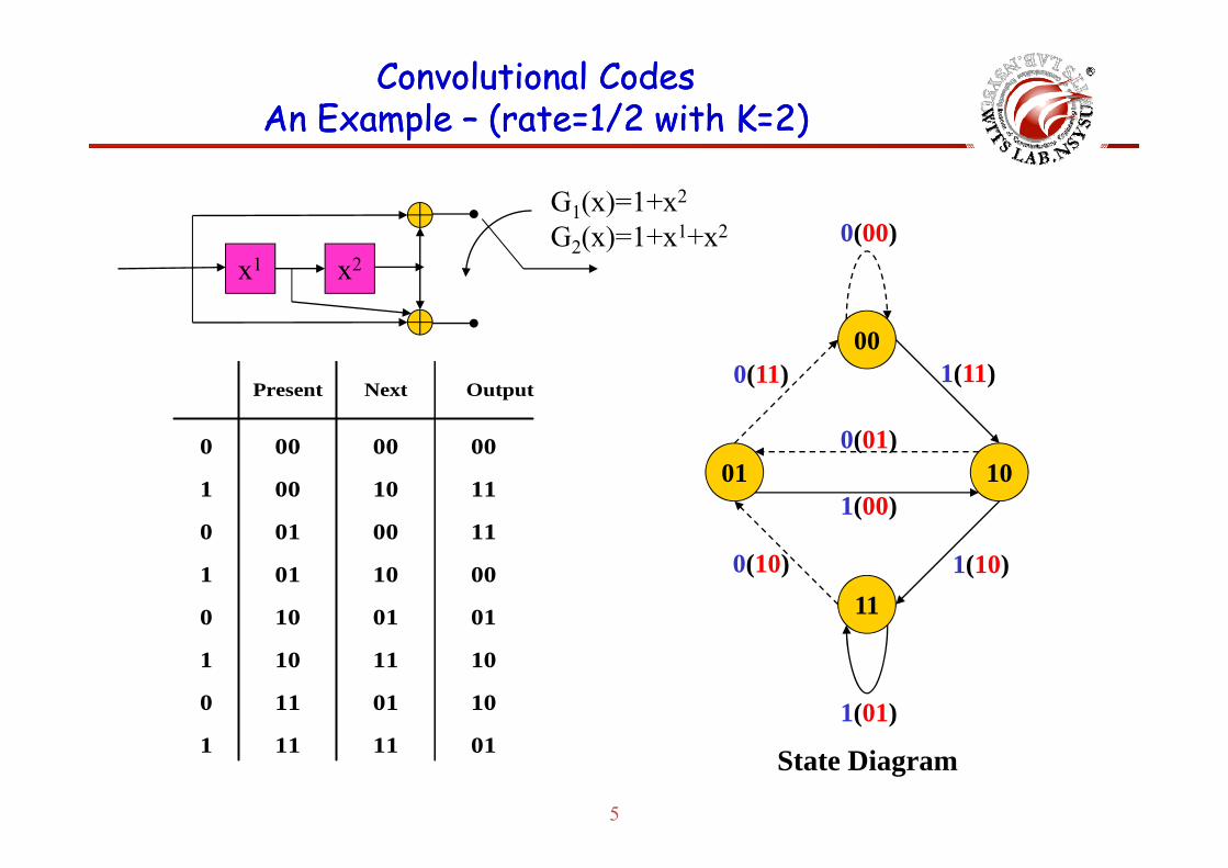
ConvolutionalConvolutional CodesCodesAn Example An Example –– (rate=1/2 with K=2)(rate=1/2 with K=2)pp
G1(x)=1+x2
G (x)=1+x1+x2 0(00)x1 x2
G2(x)=1+x1+x2
00
0(00)
Present Next Output
001(11)
0(01)
0(11)
00 000 00
1 00 10 11
010 00 11
01 100(01)
1(00)010
1
0
01
00
10
10 01
11
00
01 110(10) 1(10)
1
0
10 11
11 01
10
10 1(01)
5
1 11 11 01 State Diagram

Trellis Diagram RepresentationTrellis Diagram Representation
00 00 00 00 00 00 00 000(00) 0(00) 0(00)0(00)0(00) 0(00) 0(00)00 00 00 00 00 00 00 00
01 01 01 01 01
10 10 10 10 10
11 11 11 111(01) 1(01) 1(01)
6
Trellis termination: K tail bits with value 0 are usually added to the end of the code.
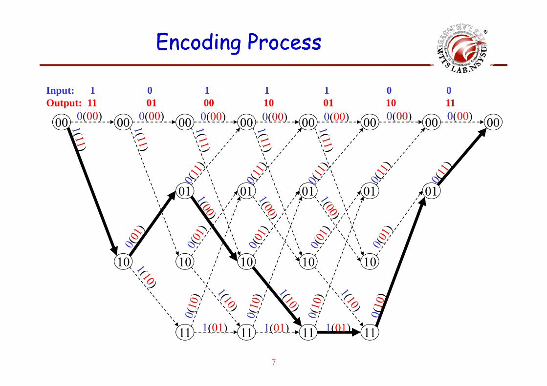
Encoding ProcessEncoding Process
Input: 1 0 1 1 1 0 0Output: 11 01 00 10 01 10 11
00 00 00 00 00 00 00 000(00) 0(00) 0(00)0(00)0(00) 0(00) 0(00)Output: 11 01 00 10 01 10 11
01 01 01 01 0101 01 01 01 01
10 10 10 10 10
1(01) 1(01) 1(01)
7
11 11 11 111(01) 1(01) 1(01)
ViterbiViterbi Decoding AlgorithmDecoding Algorithm
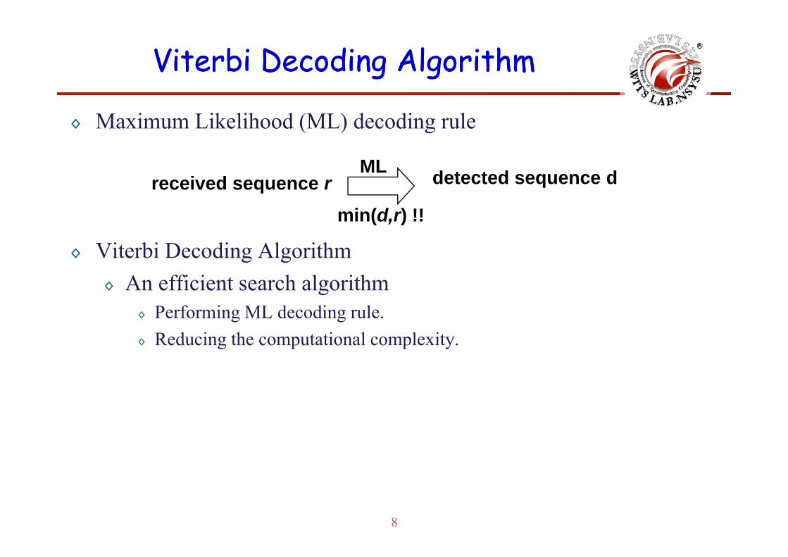
◊ Maximum Likelihood (ML) decoding rule
received sequence rML detected sequence d
min(d r) !!
◊ Viterbi Decoding AlgorithmA ffi i t h l ith
min(d,r) !!
◊ An efficient search algorithm◊ Performing ML decoding rule.◊ Reducing the computational complexity◊ Reducing the computational complexity.
8

ViterbiViterbi Decoding AlgorithmDecoding Algorithm
◊ Basic concept◊ Generate the code trellis at the decoder◊ Generate the code trellis at the decoder◊ The decoder penetrates through the code trellis level by level in
search for the transmitted code sequencesearch for the transmitted code sequence◊ At each level of the trellis, the decoder computes and compares
the metrics of all the partial paths entering a nodethe metrics of all the partial paths entering a node◊ The decoder stores the partial path with the larger metric and
eliminates all the other partial paths. The stored partial path is p p p pcalled the survivor.
9
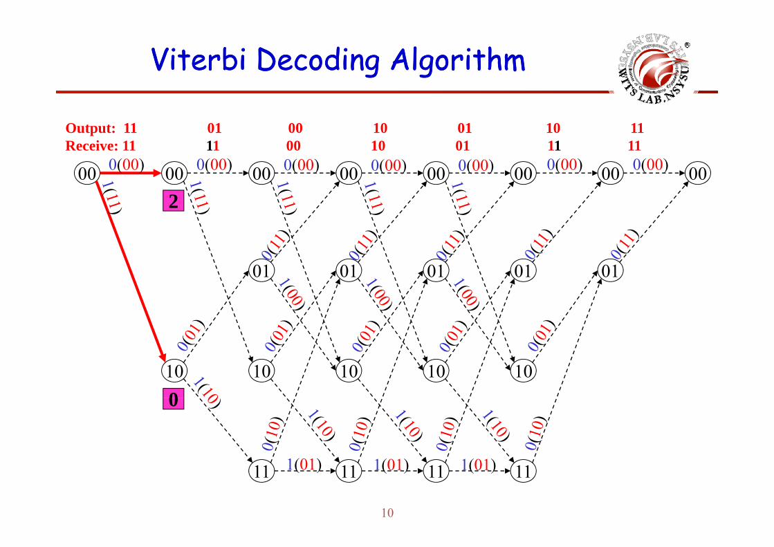
ViterbiViterbi Decoding AlgorithmDecoding Algorithm
Output: 11 01 00 10 01 10 11Receive: 11 11 00 10 01 11 11
00 00 00 00 00 00 00 000(00) 0(00) 0(00)0(00)0(00) 0(00) 0(00)Receive: 11 11 00 10 01 11 11
2
01 01 01 01 0101 01 01 01 01
10 10 10 10 100
1(01) 1(01) 1(01)
0
10
11 11 11 111(01) 1(01) 1(01)
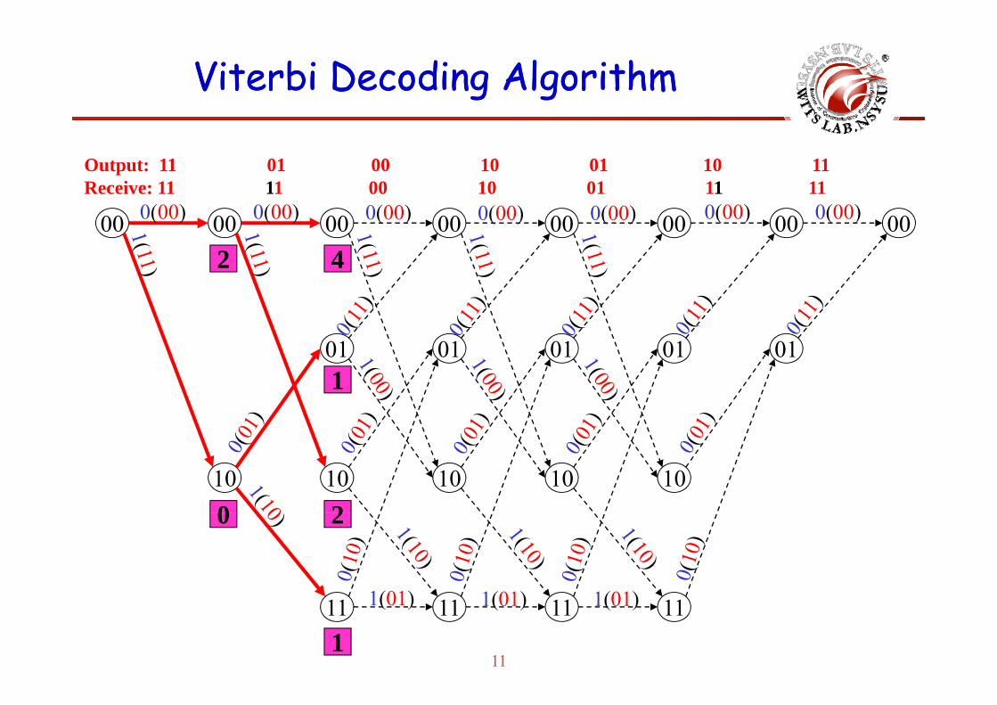
ViterbiViterbi Decoding AlgorithmDecoding Algorithm
Output: 11 01 00 10 01 10 11Receive: 11 11 00 10 01 11 11
00 00 00 00 00 00 00 000(00) 0(00) 0(00)0(00)0(00) 0(00) 0(00)Receive: 11 11 00 10 01 11 11
2 4
01 01 01 01 0101 01 01 01 011
10 10 10 10 100 2
1(01) 1(01) 1(01)
0 2
11
11 11 11 111(01) 1(01) 1(01)
1
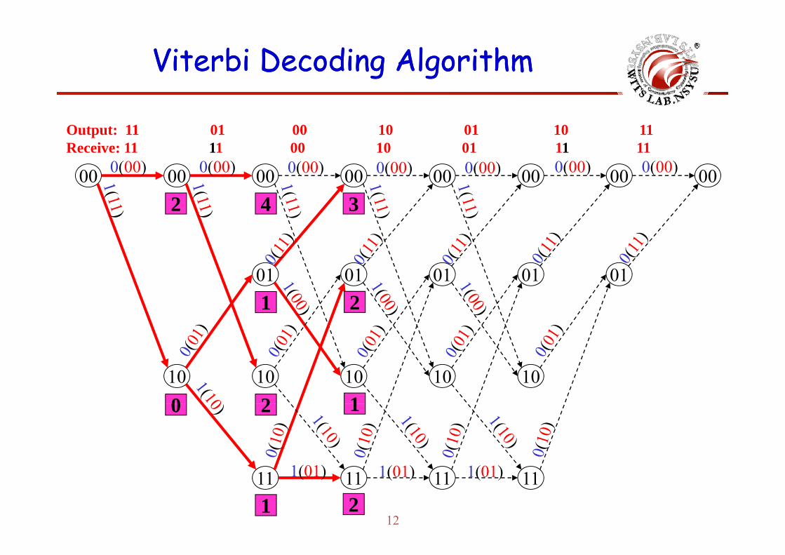
ViterbiViterbi Decoding AlgorithmDecoding Algorithm
Output: 11 01 00 10 01 10 11Receive: 11 11 00 10 01 11 11
00 00 00 00 00 00 00 000(00) 0(00) 0(00)0(00)0(00) 0(00) 0(00)Receive: 11 11 00 10 01 11 11
2 4 3
01 01 01 01 0101 01 01 01 011 2
10 10 10 10 100 2 1
1(01) 1(01) 1(01)
0 2 1
12
11 11 11 111(01) 1(01) 1(01)
1 2

ViterbiViterbi Decoding AlgorithmDecoding Algorithm
Output: 11 01 00 10 01 10 11Receive: 11 11 00 10 01 11 11
00 00 00 00 00 00 00 000(00) 0(00) 0(00)0(00)0(00) 0(00) 0(00)Receive: 11 11 00 10 01 11 11
2 4 3 3
01 01 01 01 0101 01 01 01 011 2 2
10 10 10 10 100 2 1 3
1(01) 1(01) 1(01)
0 2 1 3
13
11 11 11 111(01) 1(01) 1(01)
1 2 1

ViterbiViterbi Decoding AlgorithmDecoding Algorithm
Output: 11 01 00 10 01 10 11Receive: 11 11 00 10 01 11 11
00 00 00 00 00 00 00 000(00) 0(00) 0(00)0(00)0(00) 0(00) 0(00)Receive: 11 11 00 10 01 11 11
2 4 3 3 3
01 01 01 01 0101 01 01 01 011 2 2 3
10 10 10 10 100 2 1 3 3
1(01) 1(01) 1(01)
0 2 1 3 3
14
11 11 11 111(01) 1(01) 1(01)
1 2 1 1

ViterbiViterbi Decoding AlgorithmDecoding Algorithm
Output: 11 01 00 10 01 10 11Receive: 11 11 00 10 01 11 11
00 00 00 00 00 00 00 000(00) 0(00) 0(00)0(00)0(00) 0(00) 0(00)Receive: 11 11 00 10 01 11 11
2 4 3 3 3 3
01 01 01 01 0101 01 01 01 011 2 2 3 2
10 10 10 10 100 2 1 3 3
1(01) 1(01) 1(01)
0 2 1 3 3
15
11 11 11 111(01) 1(01) 1(01)
1 2 1 1
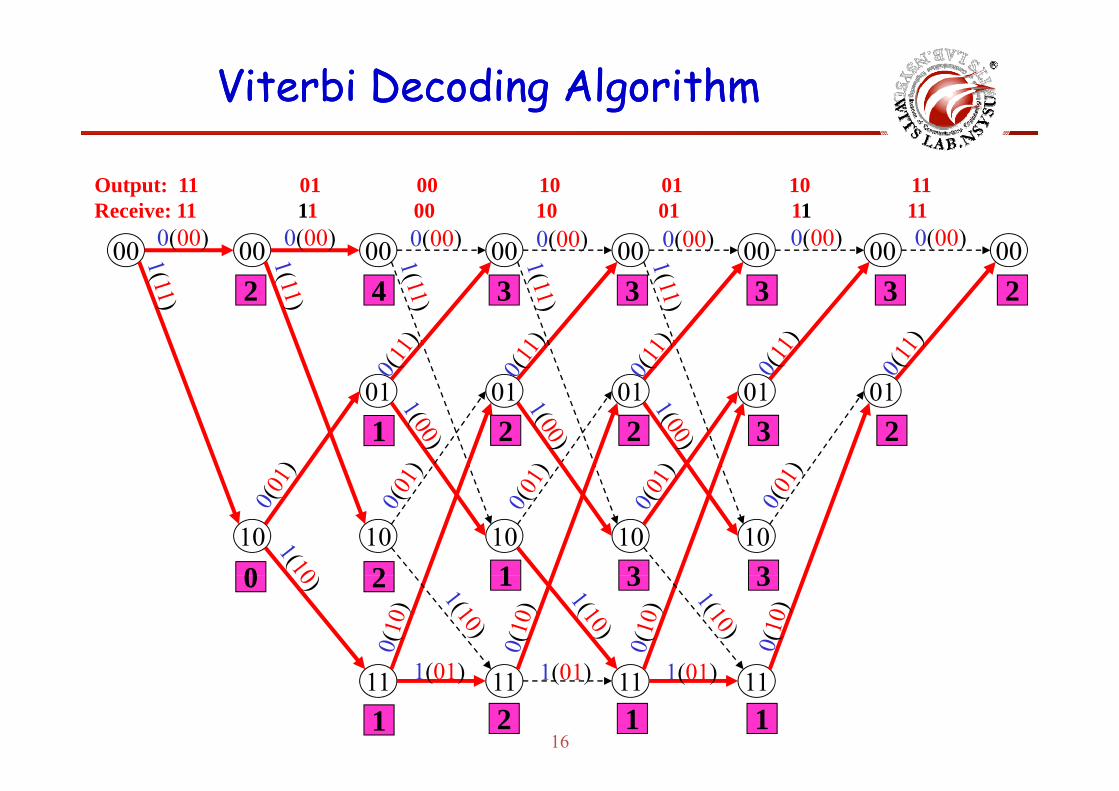
ViterbiViterbi Decoding AlgorithmDecoding Algorithm
Output: 11 01 00 10 01 10 11Receive: 11 11 00 10 01 11 11
00 00 00 00 00 00 00 000(00) 0(00) 0(00)0(00)0(00) 0(00) 0(00)Receive: 11 11 00 10 01 11 11
2 4 3 3 3 3 2
01 01 01 01 0101 01 01 01 011 2 2 3 2
10 10 10 10 100 2 1 3 3
1(01) 1(01) 1(01)
0 2 1 3 3
16
11 11 11 111(01) 1(01) 1(01)
1 2 1 1
ViterbiViterbi Decoding AlgorithmDecoding Algorithm
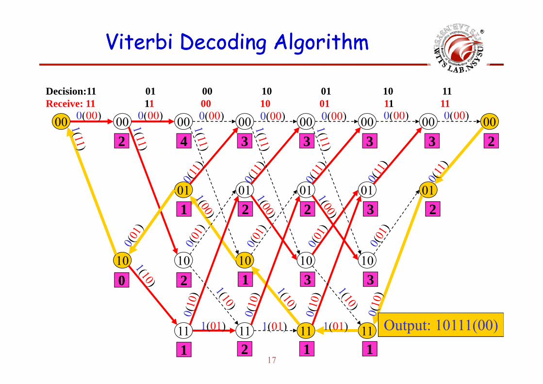
Decision:11 01 00 10 01 10 11Receive: 11 11 00 10 01 11 11
00 00 00 00 00 00 00 000(00) 0(00) 0(00)0(00)0(00) 0(00) 0(00)Receive: 11 11 00 10 01 11 11
2 4 3 3 3 3 2
01 01 01 01 0101 01 01 01 011 2 2 3 2
10 10 10 10 100 2 1 3 3
1(01) 1(01) 1(01)
0 2 1 3 3
O t t 10111(00)
17
11 11 11 111(01) 1(01) 1(01)
1 2 1 1
Output: 10111(00)

ConvolutionalConvolutional CodesCodes
Wireless Information Transmission System Lab.Wireless Information Transmission System Lab.Institute of Communications EngineeringInstitute of Communications Engineeringg gg gNational Sun National Sun YatYat--sensen UniversityUniversity
ConvolutionalConvolutional CodeCode
◊ Convolutional codes differ from block codes in that the encoder contains memory and the n encoder outputs at any time unit dependcontains memory and the n encoder outputs at any time unit depend not only on the k inputs but also on m previous input blocks.
◊ An (n, k, m) convolutional code can be implemented with a k-input, ( , , ) p p ,n-output linear sequential circuit with input memory m.◊ Typically, n and k are small integers with k<n, but the memory yp y g y
order m must be made large to achieve low error probabilities.◊ In the important special case when k=1, the information sequence is
not divided into blocks and can be processed continuously.◊ Convolutional codes were first introduced by Elias in 1955 as an
l i bl k dalternative to block codes.
19

ConvolutionalConvolutional CodeCode
◊ Shortly thereafter, Wozencraft proposed sequential decoding as an efficient decoding scheme for convolutional codes and experimentalefficient decoding scheme for convolutional codes, and experimental studies soon began to appear.
◊ In 1963, Massey proposed a less efficient but simpler-to-implement , y p p p pdecoding method called threshold decoding.
◊ Then in 1967, Viterbi proposed a maximum likelihood decodingp p gscheme that was relatively easy to implement for cods with small memory orders.
◊ This scheme, called Viterbi decoding, together with improved versions of sequential decoding, led to the application of convolutional codes to deep space and satellite communication inconvolutional codes to deep-space and satellite communication in early 1970s.
20

ConvolutionalConvolutional CodeCode
◊ A convolutional code is generated by passing the information sequence to be transmitted through a linear finite-state shift registersequence to be transmitted through a linear finite state shift register.
◊ In general, the shift register consists of K (k-bit) stages and n linear algebraic function generators.g g
21
ConvolutionalConvolutional CodeCode
◊ Convolutional codesk b f bi hif d i h d i◊ k = number of bits shifted into the encoder at one time◊ k=1 is usually used!!
◊ n = number of encoder output bits corresponding to the k information bits
◊ Rc = k/n = code rateK = constraint length encoder memory◊ K = constraint length, encoder memory.
◊ Each encoded bit is a function of the present input bits and h itheir past ones.
22

Encoding of Encoding of ConvolutionalConvolutional CodeCode
◊ Example 1:C id th bi l ti l d ith t i t l th◊ Consider the binary convolutional encoder with constraint length K=3, k=1, and n=3.The generators are: g =[100] g =[101] and g =[111]◊ The generators are: g1=[100], g2=[101], and g3=[111].
◊ The generators are more conveniently given in octal form as (4 5 7)(4,5,7).
23
Encoding of Encoding of ConvolutionalConvolutional CodeCode
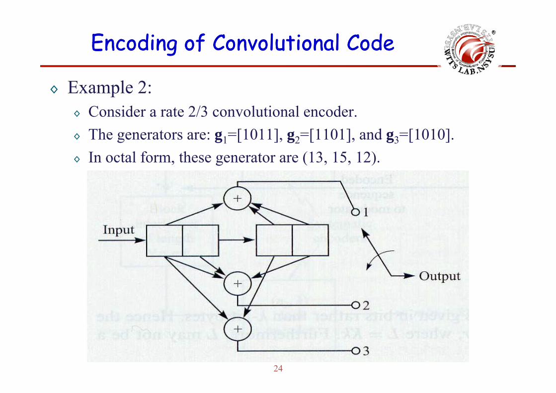
◊ Example 2:C id t 2/3 l ti l d◊ Consider a rate 2/3 convolutional encoder.
◊ The generators are: g1=[1011], g2=[1101], and g3=[1010].I l f h (13 15 12)◊ In octal form, these generator are (13, 15, 12).
24

Representations of Representations of ConvolutionalConvolutional CodeCode
◊ There are three alternative methods that are often used to describe a convolutional code:describe a convolutional code:◊ Tree diagram◊ Trellis diagram◊ State disgramg
25

Representations of Representations of ConvolutionalConvolutional CodeCode
◊ Tree diagramh h di i h i h◊ Note that the tree diagram in the right
repeats itself after the third stage.◊ This is consistent with the fact that◊ This is consistent with the fact that
the constraint length K=3.◊ The output sequence at each stage is p q g
determined by the input bit and the two previous input bits.I th d t th t th 3◊ In other words, we may sat that the 3-bit output sequence for each input bit is determined by the input bit and the y pfour possible states of the shift register, denoted as a=00, b=01, c=10, and d=11 T di f 1/3
26
and d=11. Tree diagram for rate 1/3,K=3 convolutional code.

Representations of Representations of ConvolutionalConvolutional CodeCode
◊ Trellis diagram
(00)
(01)
(10)
(11)
27
Tree diagram for rate 1/3, K=3 convolutional code.

Representations of Representations of ConvolutionalConvolutional CodeCode
◊ State diagram
0 1 a a a c⎯⎯→ ⎯⎯→0 1
0 1
b a b cc b c d⎯⎯→ ⎯⎯→
→ →0 1
c b c dd b d d⎯⎯→ ⎯⎯→
⎯⎯→ ⎯⎯→
St t di f t 1/3
28
State diagram for rate 1/3,K=3 convolutional code.

Representations of Representations of ConvolutionalConvolutional CodeCode
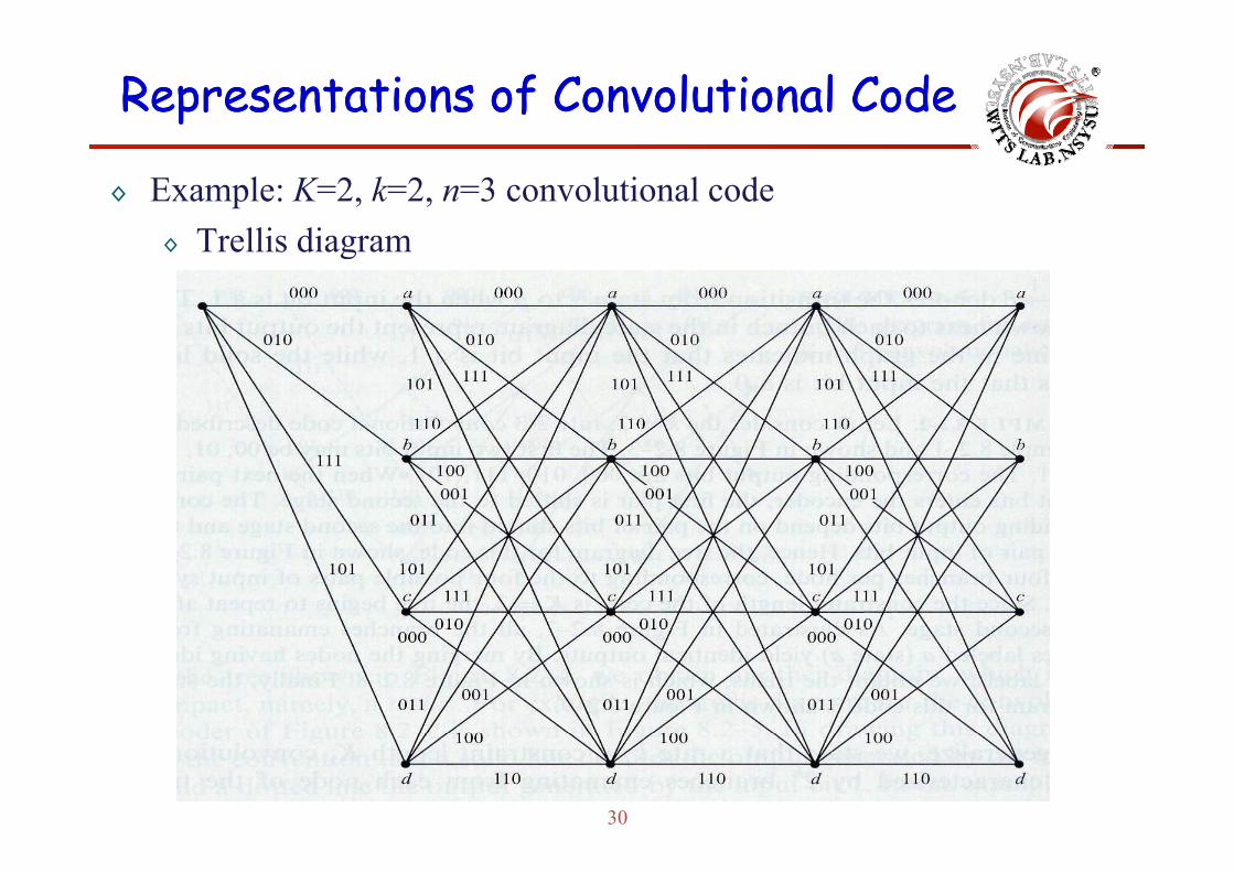
◊ Example: K=2, k=2, n=3 convolutional code◊ Tree diagram◊ Tree diagram
29
Representations of Representations of ConvolutionalConvolutional CodeCode
◊ Example: K=2, k=2, n=3 convolutional code◊ Trellis diagram◊ Trellis diagram
30

Representations of Representations of ConvolutionalConvolutional CodeCode
◊ Example: K=2, k=2, n=3 convolutional codeSt t di◊ State diagram
31

Representations of Representations of ConvolutionalConvolutional CodeCode
◊ In general, we state that a rate k/n, constraint length K, convolutional code is characterized by 2k branchesconvolutional code is characterized by 2k branches emanating from each node of the tree diagram.
h lli d h di h h 2k(K 1) ibl◊ The trellis and the state diagrams each have 2k(K-1) possible states.
◊ There are 2k branches entering each state and 2k branches leaving each state.
32

Encoding of Encoding of ConvolutionalConvolutional CodesCodes
Example: A (2, 1, 3) binary convolutional codes:
◊ the encoder consists of an m= 3-stage shift register together with n=2 modulo-2 adders and a multiplexer for serializing the encoder outputs.modulo 2 adders and a multiplexer for serializing the encoder outputs.
◊ The mod-2 adders can be implemented as EXCLUSIVE-OR gates.◊ Since mod-2 addition is a linear operation, the encoder is a linear ◊ S ce od add t o s a ea ope at o , t e e code s a ea
feedforward shift register.◊ All convolutional encoders can be implemented using a linear
33
p gfeedforward shift register of this type.
Encoding of Encoding of ConvolutionalConvolutional CodesCodes
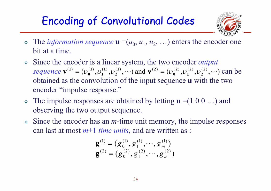
◊ The information sequence u =(u0, u1, u2, …) enters the encoder one bit at a timebit at a time.
◊ Since the encoder is a linear system, the two encoder outputsequence can be ),,,(and),,,( )()()()()()()()( 2
22
12
021
21
11
01 vv υυυυυυ ==q
obtained as the convolution of the input sequence u with the two encoder “impulse response.”
),,,(),,,( 210210
◊ The impulse responses are obtained by letting u =(1 0 0 …) and observing the two output sequence.
◊ Since the encoder has an m-time unit memory, the impulse responses can last at most m+1 time units, and are written as :
),,,(),,,()2()2(
1)2(
0)2(
)1()1(1
)1(0
)1(
m
m
gggggg
==
gg
34

Encoding of Encoding of ConvolutionalConvolutional CodesCodes
◊ The encoder of the binary (2, 1, 3) code is )1101()1( =g
The impulse response g(1) and g(2) are called the generator sequences)1 1 1 1()1 1 0 1(
)2(
)(
==
gg
p p g g g qof the code.
◊ The encoding equations can now be written as )1()1(
g q
h * d t di t l ti d ll ti d 2
)2()2(
)1()1(
guvguv∗=∗=
where * denotes discrete convolution and all operations are mod-2.◊ The convolution operation implies that for all l ≥ 0,
m
where
( ) ( ) ( ) ( ) ( )0 1 1
0, 1, 2,.j j j j j
l l i i l l l m mi
u g u g u g u g jυ − − −=
= = + + + =∑0 for allu l i= <
35
where 0 for all .l iu l i− = <

Encoding of Encoding of ConvolutionalConvolutional CodesCodes
◊ Hence, for the encoder of the binary (2,1,3) code, )1(
as can easil be erified b direct inspection of the encoding circ it321
)2(32
)1( −−−
−−
+++=++=
lllll
llll
uuuuuuu
υυ
as can easily be verified by direct inspection of the encoding circuit. ◊ After encoding, the two output sequences are multiplexed into a
signal sequence called the code word for transmission over thesignal sequence, called the code word, for transmission over the channel.
◊ The code word is given by◊ The code word is given by
).,,,( )2(2
)1(2
)2(1
)1(1
)2(0
)1(0 υυυυυυ=v
36
Encoding of Encoding of ConvolutionalConvolutional CodesCodes
◊ Example 10.1L t th i f ti (1 0 1 1 1) Th th t t◊ Let the information sequence u = (1 0 1 1 1). Then the output sequences are
1)000000(11)10(11)1101()1( =∗=v
and the code word is1) 0 1 1 1 0 1 (11) 1 1 (11) 1 1 0 1(
1) 0 0 0 0 0 0 (11) 1 0 (11) 1 1 0 1((2)
)(
=∗==∗=
vv
and the code word is 1). 1 0, 0 1, 0 1, 0 1, 0 0, 0 1, 0 1, (1=v
37

Encoding of Encoding of ConvolutionalConvolutional CodesCodes
◊ If the generator sequence g(1) and g(2) are interlaced and then arranged in the matrixg
⎥⎥⎤
⎢⎢⎡
)2()1()2()1()2()1()2()1(
)2()1()2(2
)1(2
)2(1
)1(1
)2(0
)1(0 mm
gggggggggggggggg
⎥⎥⎥⎥
⎦⎢⎢⎢⎢
⎣
=−−−−
−−)2()1()2(
1)1(1
)2(2
)1(2
)2(0
)1(0
)()()(1
)(1
)(1
)(1
)(0
)(0
mmmmmm
mmmm
gggggggggggggggg
G
where the blank areas are all zeros, the encoding equations can be itt i t i f G
⎥⎦⎢⎣
rewritten in matrix form as v = uG.◊ G is called the generator matrix of the code. Note that each row of
G is identical to the preceding row but shifted n = 2 places to right,G is identical to the preceding row but shifted n 2 places to right, and the G is a semi-infinite matrix, corresponding to the fact that the information sequence u is of arbitrary length.
38

Encoding of Encoding of ConvolutionalConvolutional CodesCodes
◊ If u has finite length L, then G has L rows and 2(m+L) columns, and v has length 2(m + L).g ( )
◊ Example 10.2◊ If u=(1 0 1 1 1) then◊ If u (1 0 1 1 1), then
11111011 ⎤⎡= uGv
111101111 11 10111
11111011
1)110(1 ⎥⎥⎥⎤
⎢⎢⎢⎡
111110111 11 11 011
111101111) 1 1 0 (1
⎥⎥⎥⎥
⎦⎢⎢⎢⎢
⎣
=
1), 1 0, 0 1, 0 1, 0 1, 0 0, 0 1, 0 1, (1 11111011
=⎥⎦⎢⎣
39
agree with our previous calculation using discrete convolution.

Encoding of Encoding of ConvolutionalConvolutional CodesCodes
◊ Consider a (3, 2, 1) convolutional codes
Since k = 2, the encoder consists of two m = 1consists of two m = 1-stage shift registers together with n = 3 oge e w n 3mode-2 adders and two multiplexers.
40

Encoding of Encoding of ConvolutionalConvolutional CodesCodes
◊ The information sequence enters the encoder k = 2 bits at a time, and can be written ascan be written as
h i
),,,( )2(2
)1(2
)2(1
)1(1
)2(0
)1(0 uuuuuu=u
)( )1()1()1()1(or as the two input sequences
◊ There are three generator sequences corresponding to each input),,,(
),,,()2(
2)2(
1)2(
0(2)
)1(2
)1(1
)1(0
)1(
uuuuuu
==
uu
◊ There are three generator sequences corresponding to each input sequence.
◊ Let represent the generator sequence)( )()(1
)(0
)( jjjj gggg =◊ Let represent the generator sequence corresponding to input i and output j, the generator sequence of the (3, 2, 1) convolutional codes are
),,,( ,1,0, miiii gggg
),01(),01(),10(),1 1( 1), 0( 1), 1(
(3)2
(2)2
)1(2
(3)1
(2)1
)1(1
======
gggggg
41
),0 1( ),0 1( ),1 0( 222 ggg

Encoding of Encoding of ConvolutionalConvolutional CodesCodes
◊ And the encoding equations can be written as )1()2()1()1()1(
)3()2()3()1()3(
)2(2
)2()2(1
)1()2(
)1(2
)2()1(1
)1()1(
guguvguguvguguv
∗+∗∗+∗=∗+∗=
◊ The convolution operation implies that
)(2
)()(1
)()( guguv ∗+∗=
)2()1()1()1(
)1()2()1()3(
)1(1
)2()2(
)2(1
)1(1
)1()1(
−
−−
+++=
++=
lll
llll
uuuuu
uuu
υυυ
◊ After multiplexing, the code word is given by ,)(
1)()()(
−++= llll uuuυ
).,,,( )3(2
)2(2
)1(2
)3(1
)2(1
)1(1
)3(0
)2(0
)1(0 υυυυυυυυυ=v
42
Encoding of Encoding of ConvolutionalConvolutional CodesCodes
◊ Example 10.3If (1) (1 0 1) d (2) (1 1 0) th◊ If u(1) = (1 0 1) and u(2) = (1 1 0), then
1) 0 0 (11) (00) 1 (11) (11) 0 1()2(
)1( =∗+∗=v
d1) 1 0 (00) (10) 1 (11) (11) 0 1(1) 0 0 (10) (10) 1 (11) (01) 0 1(
)3(
)2(
=∗+∗==∗+∗=
vv
and ).1 1 1 ,1 0 0 , 0 0 0 ,0 1 1(=v
43

Encoding of Encoding of ConvolutionalConvolutional CodesCodes
◊ The generator matrix of a (3, 2, m) code is
⎤⎡ )3()2()1()3()2()1()3()2()1(
⎥⎥⎥⎤
⎢⎢⎢⎡
)3()2()1()3()2()1()3()2()1(
)3(,2
)2(,2
)1(,2
)3(1,2
)2(1,2
)1(1,2
)3(0,2
)2(0,2
)1(0,2
)3(,1
)2(,1
)1(,1
)3(1,1
)2(1,1
)1(1,1
)3(0,1
)2(0,1
)1(0,1
mmm
mmm
gggggggggggggggggg
⎥⎥⎥⎥
⎢⎢⎢⎢=
−−−
−−−)3(
,2)2(
,2)1(
,2)3(
1,2)2(
1,2)1(
1,2)3(0,2
)2(0,2
)1(0,2
)3(,1
)2(,1
)1(,1
)3(1,1
)2(1,1
)1(1,1
)3(0,1
)2(0,1
)1(0,1
mmmmmm
mmmmmm
ggggggggggggggggggG
and the encoding equation in matrix are again given by v = uG.
⎥⎦⎢⎣
◊ Note that each set of k = 2 rows of G is identical to the preceding set of rows but shifted n = 3 places to right.
44

Encoding of Encoding of ConvolutionalConvolutional CodesCodes
◊ Example 10.4If u(1) = (1 0 1) and u(2) = (1 1 0) then u = (1 1 0 1 1 0) and◊ If u(1) = (1 0 1) and u(2) = (1 1 0), then u = (1 1, 0 1, 1 0) and
111101 ⎤⎡= uGv
1111010 0 11 1 01 1 11 0 1
⎥⎥⎥⎤
⎢⎢⎢⎡
1 1 11 0 10 0 11 1 01 1 11 0 1
0) 11, 01, (1
⎥⎥⎥⎥⎥
⎢⎢⎢⎢⎢
=
1), 1 1 1, 0 0 0, 0 0 0, 1 (1 0 0 11 1 0
=⎥⎥⎦⎢
⎢⎣
it agree with our previous calculation using discrete convolution.
45

Encoding of Encoding of ConvolutionalConvolutional CodesCodes
◊ In particular, the encoder now contains k shift registers, not all of which must have the same lengthwhich must have the same length.
◊ If Ki is the length of the ith shift register, then the encoder memory order m is defined as max im K
1max ii k
m K≤ ≤
An example of a (4, 3, 2) p ( , , )convolutional encoder in which the shift register l h 0 1 d 2length are 0, 1, and 2.
46

Encoding of Encoding of ConvolutionalConvolutional CodesCodes
◊ The overall constraint length is defined as nA≡n(m+1).◊ Since each information bit remains in the encoder for up to m+1 time◊ Since each information bit remains in the encoder for up to m+1 time
units, and during each time unit can affect any of the n encoder outputs, nA can be interpreted as the maximum number of encoder p , A poutputs that can be affected by a signal information bit.
◊ For example, the constraint length of the (2,1,3), (3,2,1), and (4,3,2) p g ( ) ( ) ( )convolutional codes are 8, 6, and 12, respectively.
◊ Note that different books or papers may have different definitions for constraint length.
47
Encoding of Encoding of ConvolutionalConvolutional CodesCodes
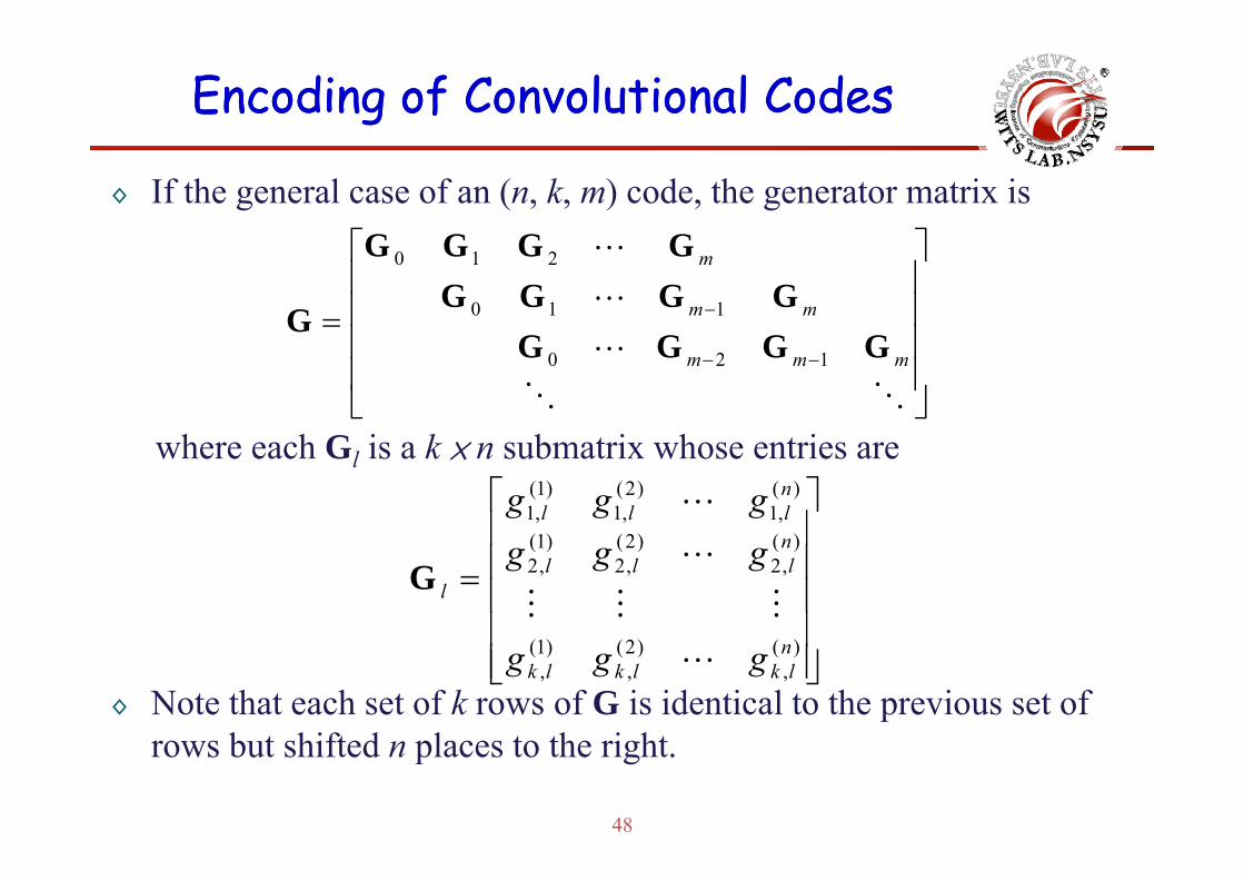
◊ If the general case of an (n, k, m) code, the generator matrix is ⎤⎡ GGGG
⎥⎥⎥⎤
⎢⎢⎢⎡
= − mm
m
GGGGGGGG
GGGG
G 110
210
h h G i k b t i h t i
⎥⎥
⎦⎢⎢
⎣−− mmm GGGG 120
where each Gl is a k × n submatrix whose entries are
⎥⎤
⎢⎡
)()2()1(
)(,1
)2(,1
)1(,1
n
nlll ggg
⎥⎥⎥⎥
⎢⎢⎢⎢
=
)()2()1(
)(,2
)2(,2
)1(,2
nlll
l
gggG
◊ Note that each set of k rows of G is identical to the previous set of b t hift d l t th i ht
⎥⎥⎦⎢
⎢⎣
)(,
)2(,
)1(,
nlklklk ggg
48
rows but shifted n places to the right.

Encoding of Encoding of ConvolutionalConvolutional CodesCodes
◊ For an information sequence)()( )()2()1()()2()1( kkuuu
and the code wordis gi en b v uG
),,(),,( )(1
)(1
)(1
)(0
)(0
)(010
kk uuuuuu== uuu),,(),,( )(
1)2(
1)1(
1)(
0)2(
0)1(
010nn υυυυυυ== vvv
is given by v = uG. ◊ Since the code word v is a linear combination of rows of the
generator matrix G an (n k m) convolutional code is a linear codegenerator matrix G, an (n, k, m) convolutional code is a linear code.
49

Encoding of Encoding of ConvolutionalConvolutional CodesCodes
◊ A convolutional encoder generates n encoded bits for each kinformation bits and R = k/n is called the code rateinformation bits, and R k/n is called the code rate.
◊ For an k·L finite length information sequence, the corresponding code word has length n(L + m), where the final n·m outputs are g ( ), pgenerated after the last nonzero information block has entered the encoder.
◊ Viewing a convolutional code as a linear block code with generator matrix G, the block code rate is given by kL/n(L + m), the ratio of th b f i f ti bit t th l th f th d dthe number of information bits to the length of the code word.
◊ If L » m, then L/(L + m) ≈ 1, and the block code rate and convolutional code are approximately equalconvolutional code are approximately equal .
50

Encoding of Encoding of ConvolutionalConvolutional CodesCodes
◊ In a linear system, time-domain operations involving convolutioncan be replaced by more convenient transform-domain operationscan be replaced by more convenient transform domain operationsinvolving polynomial multiplication.
◊ Since a convolutional encoder is a linear system, each sequence in y , qthe encoding equations can be replaced by corresponding polynomial, and the convolution operation replaced by polynomial multiplication.
◊ In the polynomial representation of a binary sequence, the sequence it lf i t b th ffi i t f th l i litself is represent by the coefficients of the polynomial.
◊ For example, for a (2, 1, m) code, the encoding equations become
2),()()()()()(
)2()2(
)1()1(
DDDDDD
guvguv
==
51
where u(D) = u0 + u1D + u2D2 + ··· is the information sequence.

Encoding of Encoding of ConvolutionalConvolutional CodesCodes
◊ The encoded sequences are2)1()1()1()1( )( DDD
The t l i l of the code are+++=+++=2)2(
2)2(
1)2(
0)2(
2)1(2
)1(1
)1(0
)1(
)()(
DDDDDD
υυυυυυ
vv
◊ The generator polynomials of the code are
m
mm
DDDDgDggD)2()2()2()2(
)1()1(1
)1(0
)1(
)()(
++++++=g
and all operations are modulo-2.Aft lti l i th d d b
mm DgDggD )2()2(
1)2(
0)2( )( +++=g
◊ After multiplexing, the code word become
h i d i D b i d d l d h)()()( 2)2(2)1( DDDD vvv +=
the indeterminate D can be interpreted as a delay operator, and the power of D denoting the number of time units a bit is delayed with respect to the initial bit
52
respect to the initial bit.

Encoding of Encoding of ConvolutionalConvolutional CodesCodes
◊ Example 10.6For the previous (2 1 3) convolutional code the generator◊ For the previous (2, 1, 3) convolutional code, the generator polynomials are g(1)(D) = 1+D2+D3 and g(2)(D) = 1+D+D2+D3.
◊ For the information sequence u(D) = 1+D2+D3+D4, the encoding ◊ o e o a o seque ce u( ) , e e cod gequation are
1)1)(1()( 732432)1( DDDDDDD +=+++++=v
d th d d i,1
)1)(1()(7543
32432)2(
DDDDDDDDDDDD
+++++=++++++=v
and the code word is
( ) (1) 2 (2) 2 3 7 9 11 14 15( ) ( ) 1 .D D D D D D D D D D D= + = + + + + + + +v v v
◊ Note that the result is the same as previously computed using convolution and matrix multiplication.
53

Encoding of Encoding of ConvolutionalConvolutional CodesCodes
◊ Since the encoder is a linear system, and u(i)(D) is the ith input sequence and v(j)(D) is the jth output sequence the generatorsequence and v (D) is the jth output sequence, the generator polynomial can be interpreted as the encoder transfer function relating input i to output j.
( ) ( )Djig
◊ As with k-input, n-output linear system, there are a total of k·ntransfer functions.
◊ These can be represented by the k × n transfer function matrix
( ) ( ) ( ) ( ) ( ) ( )1 2 nD D D⎡ ⎤g g g
( )
( ) ( ) ( ) ( ) ( ) ( )( ) ( ) ( ) ( ) ( ) ( )1 1 1
1 22 2 2D
n
D D D
D D D
⎡ ⎤⎢ ⎥⎢ ⎥
= ⎢ ⎥
g g g
g g gG ( )
( ) ( ) ( ) ( ) ( ) ( )1 2 nk k kD D D
⎢ ⎥⎢ ⎥⎢ ⎥⎣ ⎦g g g
54
( ) ( ) ( )⎣ ⎦
Encoding of Encoding of ConvolutionalConvolutional CodesCodes
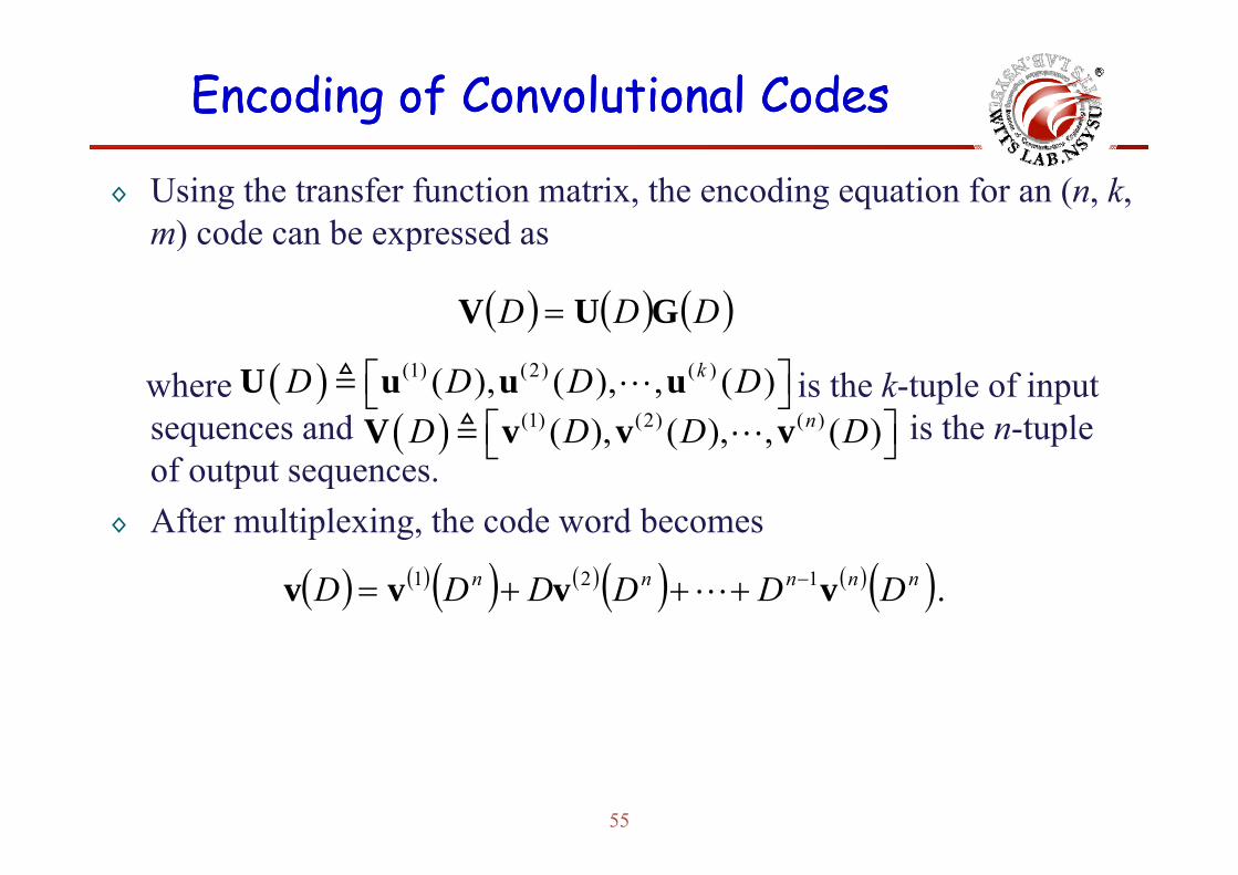
◊ Using the transfer function matrix, the encoding equation for an (n, k, m) code can be expressed asm) code can be expressed as
( ) ( ) ( )DDD GUV =
where is the k-tuple of input sequences and is the n-tuple
( ) (1) (2) ( )( ), ( ), , ( )kD D D D⎡ ⎤⎣ ⎦U u u u( ) (1) (2) ( )( ) ( ) ( )nD D D D⎡ ⎤⎣ ⎦V v v vsequences and is the n tuple
of output sequences.◊ After multiplexing, the code word becomes
( ) ( ), ( ), , ( )D D D D⎡ ⎤⎣ ⎦V v v v
p g,
( ) ( ) ( ) ( ) ( ) ( ) ( ). 121 nnnnn DDDDDD vvvv −+++=
55

Encoding of Encoding of ConvolutionalConvolutional CodesCodes
◊ Example 10.7For the previous (3 2 1) convolutional code◊ For the previous (3, 2, 1) convolutional code
( ) ⎥⎦
⎤⎢⎣
⎡ ++=
1111
DDDD
DG1 0 1 1 1 10 1 1 1 0 0⎡ ⎤⎢ ⎥⎣ ⎦
◊ For the input sequences u(1)(D) = 1+D2 and u(2)(D)=1+D, the encoding equations are
⎥⎦
⎢⎣ 11D 0 1 1 1 0 0⎣ ⎦
q
( ) ( ) ( ) ( ) ( ) ( ) ( )[ ] [ ]2321
1111
1,1,,D
DDDDDDDDD ⎥
⎦
⎤⎢⎣
⎡ ++++== vvvV
and the code word is [ ]3233 ,D1,D1 DD +++=
⎦⎣
( ) ( ) ( ) ( )9 9 6 9 2
8 9 10 11
D 1 1
1
D D D D D D
D D D D D
= + + + + +
= + + + + +
v
56

Encoding of Encoding of ConvolutionalConvolutional CodesCodes
◊ Then, we can find a means of representing the code word v(D) directly in terms of the input sequencesdirectly in terms of the input sequences.
◊ A little algebraic manipulation yields
h
( ) ( ) ( ) ( )DD in
k
i
i guv ∑=
=1
D
where
( ) ( ) ( ) ( ) ( ) ( ) ( )1 2 11 , 1 ,nn n n ni i i ig D D D D D D i k−−+ + ≤ ≤g g g
is a composite generator polynomial relating the ith input sequence to v(D)
( ) ( ) ( ) ( )i i i ig g g g
to v(D).
57

Encoding of Encoding of ConvolutionalConvolutional CodesCodes
◊ Example 10.8F th i (2 1 3) l ti l d th it◊ For the previous (2, 1, 3) convolutional codes, the composite generator polynomial is
( ) ( )d f (D) 1+D2+D3+D4 th d d i
( ) ( ) ( ) ( ) ( ) 765432221 1 DDDDDDDDDD ++++++=+= ggg
and for u(D)=1+D2+D3+D4 , the code word is
( ) ( ) ( )2 D D D=v u g( )( ) ( )4 6 8 3 4 5 6 7
3 7 9 11 14 15
1 1
1
D D D D D D D D D
D D D D D D D
= + + + ⋅ + + + + + +
again agreeing with previous calculations.
3 7 9 11 14 15 1 D D D D D D D= + + + + + + +
58
Structural Properties of Structural Properties of ConvolutionalConvolutional CodesCodes
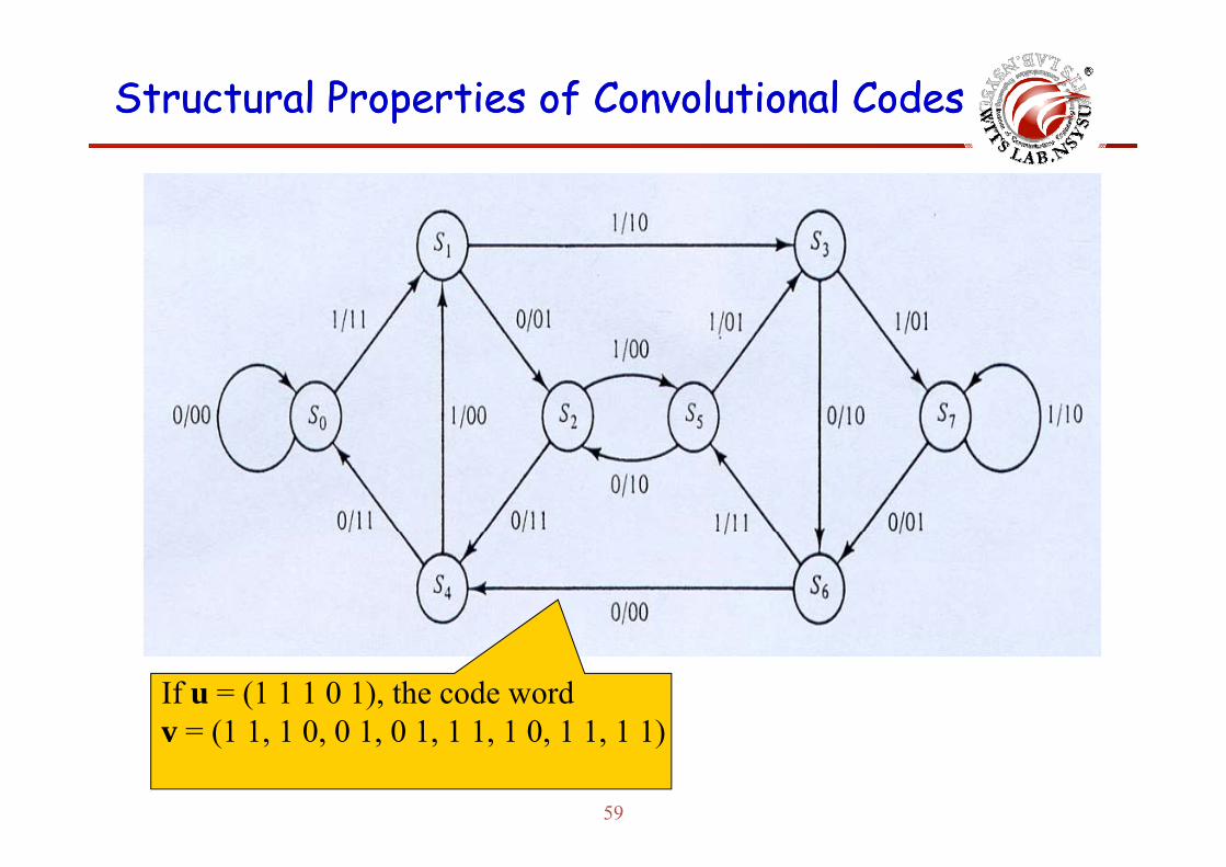
If u = (1 1 1 0 1), the code word v = (1 1 1 0 0 1 0 1 1 1 1 0 1 1 1 1)
59
v = (1 1, 1 0, 0 1, 0 1, 1 1, 1 0, 1 1, 1 1)
Structural Properties of Structural Properties of ConvolutionalConvolutional CodesCodes
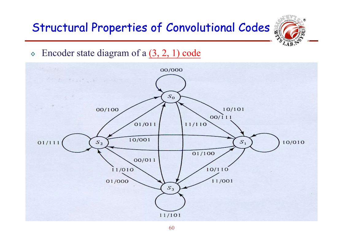
◊ Encoder state diagram of a (3, 2, 1) code
60
Structural Properties of Structural Properties of ConvolutionalConvolutional CodesCodes
◊ The state diagram can be modified to provide a complete description of the Hamming weights of all nonzero code words (i e a weightof the Hamming weights of all nonzero code words (i.e. a weight distribution function for the code).
◊ State S0 is split into an initial state and a final state, the self-loop 0 p f , paround state S0 is deleted, and each branch is labeled with a branch gain Xi ,where i is the weight of the n encoded bits on that branch.
◊ Each path connecting the initial state to the final state represents a nonzero code word that diverge from and remerge with state S0
tlexactly once.◊ The path gain is the product of the branch gains along a path, and
the weight of the associated code word is the power of X in the paththe weight of the associated code word is the power of X in the path gain.
61

Structural Properties of Structural Properties of ConvolutionalConvolutional CodesCodes
Modified encoder state diagram of a (2, 1, 3) code.
The path representing the sate sequence S S S S S S S S S
62
The path representing the sate sequence S0S1S3S7S6S5S2S4S0has path gain X2·X1·X1·X1·X2·X1·X2·X2=X12.

Structural Properties of Structural Properties of ConvolutionalConvolutional CodesCodes
Modified encoder state diagram of a (3, 2, 1) code.
The path representing the sate sequence S S S S S
63
The path representing the sate sequence S0S1S3S2S0has path gain X2·X1·X0·X1 =X12.
Structural Properties of Structural Properties of ConvolutionalConvolutional CodesCodes
◊ The weight distribution function of a code can be determined by considering the modified state diagram as a signal flow graph andconsidering the modified state diagram as a signal flow graph and applying Mason’s gain formula to compute its “generating function”
( ) iXAXT ∑
where Ai is the number of code words of weight i.
( ) ,i
ii XAXT ∑=
where Ai is the number of code words of weight i.◊ In a signal flow graph, a path connecting the initial state to the final
state which does not go through any state twice is called a forward g g y fpath.
◊ A closed path starting at any state and returning to that state without going through any other state twice is called a loop.
64

Structural Properties of Structural Properties of ConvolutionalConvolutional CodesCodes
◊ Let Ci be the gain of the ith loop.◊ A set of loops is nontouching if no state belongs to more than one◊ A set of loops is nontouching if no state belongs to more than one
loop in the set.◊ Let {i} be the set of all loops {i’ j’} be the set of all pairs of◊ Let {i} be the set of all loops, {i , j } be the set of all pairs of
nontouching loops, {i”, j”, l”} be the set of all triples of nontouching loops, and so on.g p
◊ Define ,1 ''''''''''
'''''
'
,,,
+−+−=Δ ∑∑∑ ljlji
ijji
ii
i CCCCCC
where is the sum of the loop gains, is the product of the loop gains of two nontouching loops summed over all pairs of
∑i
iC '''
'
,j
jii CC∑
CCC∑nontouching loops, is the product of the loop gains of three nontouching loops summed over all nontouching loops.
''''''''''
''
,,lj
ljii
CCC∑
65

Structural Properties of Structural Properties of ConvolutionalConvolutional CodesCodes
◊ And ∆i is defined exactly like ∆, but only for that portion of the graph not touching the ith forward path; that is all states along thegraph not touching the ith forward path; that is, all states along the ith forward path, together with all branches connected to these states, are removed from the graph when computing ∆i.
◊ Mason’s formula for computing the generating function T(X) of a graph can now be states as
( ) ,i i
i
FT X
Δ=∑
where the sum in the numerator is over all forward paths and Fi is the
( ) ,T XΔ
gain of the ith forward path.
66

Structural Properties of Structural Properties of ConvolutionalConvolutional CodesCodes
( )XCSSSSSSS SLoop = 8114256731 : 1Example (2 1 3) Code:
( )( )XCSSSSSSSLoop
XCSSSSS SLoop
=
=7
31425631
32146731
:3
: 2Example (2,1,3) Code:
There are 11 loops in the modified encoder state ( )
( )( )XCSSSSSSSSLoop
XCSSSS SLoop
p
=
=9
514673521
2414631
31425631
:5
: 4diagram.
( )( )( )XCSSSSLoop
XCSSSSSSSLoop
CSSSSSSSSoop
=
=3
861463521
514673521
:7
: 6
:5
( )( )( )XCSSSSSLoop
XCSS SLoop XCSSSSLoop
=
==
58252
71421
:9
:8 :7
( )( )( )XCSSLoop
XCSSS SLoop
XCSSSSSLoop
==
=4
103563
935673
:11 : 10
:9
67
( )XCSSLoop =1177 :11

Structural Properties of Structural Properties of ConvolutionalConvolutional CodesCodes
◊ Example (2,1,3) Code: (cont.)Th 10 i f t hi l◊ There are 10 pairs of nontouching loops :
( ) ( )42 8Loop pair 1: loop 2 loop 8 , C C X=
( ) ( )( ) ( )
( )
83 11
34 8
Loop pair 2: loop 3 loop 11
Loop pair 3: loop 4 loop 8
, C C X
, C C X
=
=
( ) ( )34 11Loop pair 4: loop 4 loop 11
Loop pair 5: loop
, C C X
=
( ) ( )( ) ( )
96 11
8
6 loop 11 , C C X=
( ) ( )( ) ( )( ) ( )
87 9
77 10
4
Loop pair 6: loop 7 loop 9
Loop pair 7: loop 7 loop 10
L i 8 l 7 l 11
, C C X
, C C X
C C X
=
=
( ) ( )( )
47 11
8
Loop pair 8: loop 7 loop 11
Loop pair 9: loop 8 loop 11
, C C X
, C
=
( )( ) ( )
211
5Loop pair 10: loop 10 loop 11
C X
C C X
=
68
( ) ( )10 11Loop pair 10: loop 10 loop 11 , C C X=

Structural Properties of Structural Properties of ConvolutionalConvolutional CodesCodes
◊ Example (2,1,3) Code : (cont.)◊ There are two triples of nontouching loops :◊ There are two triples of nontouching loops :
( ) ( )41184 11 loop 8, loop 4, loop :1 tripleLoop XCCC =
Th th t f t hi l Th f
( ) ( )811107 11 loop 10, loop 7, loop :2 tripleLoop XCCC =
◊ There are no other sets of nontouching loops. Therefore,
( )4533427381 XXXXXXXXXXX ++++++++++−=Δ ( )( )( ) 384
5247843384
21
XXXXXXXXXXXXXX
+−=+−
++++++++++
( ) 21 XXXX ++
69

Structural Properties of Structural Properties of ConvolutionalConvolutional CodesCodes
◊ Example (2,1,3) Code : (cont.)Th f d th i thi t t di◊ There are seven forward paths in this state diagram :
( ):1path Foward 121042567310 XF SSSSSSSS S =( )
( )( ):3pathFoward
:2path Foward11
720467310
XFSSSSSSSS
XF SSSSSS S
=
=
( )( )( )hd
:4path Foward
:3path Foward
8
64046310
304256310
SSSSSSSSS
XF SSSSS S
XFSSSSSSS S
=
=
( )( ) :6path Foward
:5path Foward7
604635210
85046735210
XF SSSSSSS S
XF SSSSSSSS S
=
=
( ). :7path Foward 7704210 XF SSSS S =
70

Structural Properties of Structural Properties of ConvolutionalConvolutional CodesCodes
◊ Example (2,1,3) Code : (cont.)F d th 1 d 5 t h ll t t i th h d h th◊ Forward paths 1 and 5 touch all states in the graph, and hence the sub graph not touching these paths contains no states. Therefore,
∆ = ∆ = 1∆1 = ∆5 = 1.
The subgraph not touching forward paths 3 and 6:g p g p
∆3 = ∆6 = 1 - X∆3 ∆6 1 X
71
Structural Properties of Structural Properties of ConvolutionalConvolutional CodesCodes
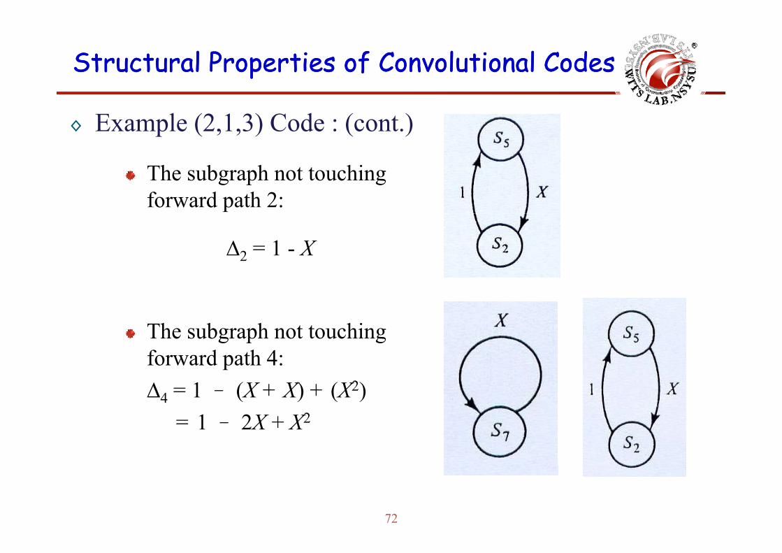
◊ Example (2,1,3) Code : (cont.)
The subgraph not touching forward path 2:
∆2 = 1 - X
The subgraph not touching g p gforward path 4:∆4 = 1 – (X + X) + (X2) 4
= 1 – 2X + X2
72

Structural Properties of Structural Properties of ConvolutionalConvolutional CodesCodes
◊ Example (2,1,3) Code : (cont.)Th b h t t hi◊ The subgraph not touching forward path 7:∆ = 1 (X + X4 + X5) + (X5)∆7 = 1 – (X + X4 + X5) + (X5)
= 1 – X – X4
73
Structural Properties of Structural Properties of ConvolutionalConvolutional CodesCodes
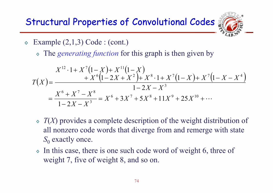
◊ Example (2,1,3) Code : (cont.)◊ The generating function for this graph is then given by◊ The generating function for this graph is then given by
( ) ( )( ) ( ) ( )
−+−+⋅477826
11712 111 XXXXX
( ) ( ) ( ) ( )−+
−−−−+−+⋅++−+
=
109876876
3
477826
25115321
11121
XXXXXXXXXX
XXXXXXXXXXT
T(X) id l t d i ti f th i ht di t ib ti f
+++++=−−
= 1098763 251153
21 XXXXX
XX
◊ T(X) provides a complete description of the weight distribution of all nonzero code words that diverge from and remerge with state S0 exactly onceS0 exactly once.
◊ In this case, there is one such code word of weight 6, three of weight 7, five of weight 8, and so on.
74
weight 7, five of weight 8, and so on.

Structural Properties of Structural Properties of ConvolutionalConvolutional CodesCodes
◊ Example (3,2,1) Code : (cont.)◊ There are eight loops six pairs of nontouching loops and one◊ There are eight loops, six pairs of nontouching loops, and one
triple of nontouching loops in the graph of previous modified encoder state diagrams : (3, 2, 1) code, and g ( , , ) ,
( )( ) ( )
16543426
3212342
XXXXXXXXXXXXXXX +++++++−=Δ
( ) ( ).221
5432
6543426
XXXXXXXXXXXX
++−−−=
−++++++
75
Structural Properties of Structural Properties of ConvolutionalConvolutional CodesCodes
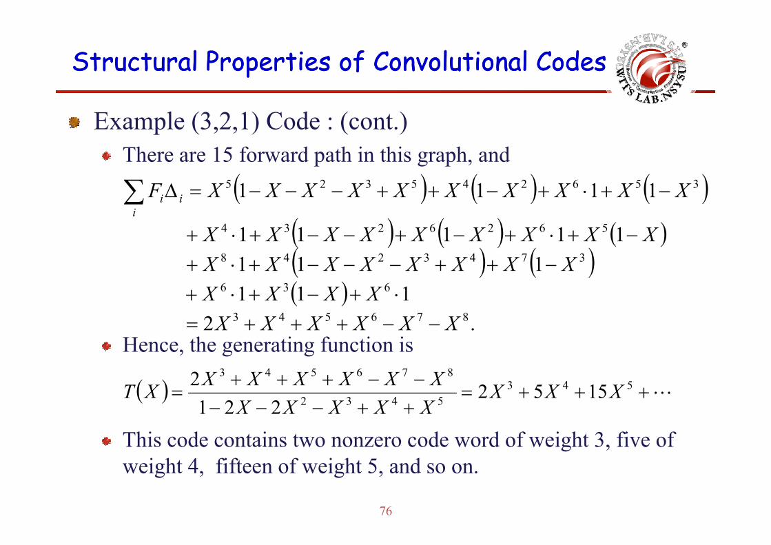
Example (3,2,1) Code : (cont.)Th 15 f d th i thi h dThere are 15 forward path in this graph, and
( ) ( ) ( )1111 356245325 XXXXXXXXXXFi
ii −+⋅+−++−−−=Δ∑( ) ( ) ( )( ) ( )111
11111 3743248
5626234
XXXXXXXXXXXXXXXXX
i
−++−−−+⋅+−+⋅+−+−−+⋅+
( ) ( )( )
.2 111
876543
636
XXXXXXXXXX
−−+++=⋅+−+⋅+
Hence, the generating function is
( ) +++=−−+++
= 543876543
15522 XXXXXXXXXXT
This code contains two nonzero code word of weight 3, five of i h fif f i h d
( ) +++++−−− 5432 1552
221XXX
XXXXXXT
76
weight 4, fifteen of weight 5, and so on.
Structural Properties of Structural Properties of ConvolutionalConvolutional CodesCodes
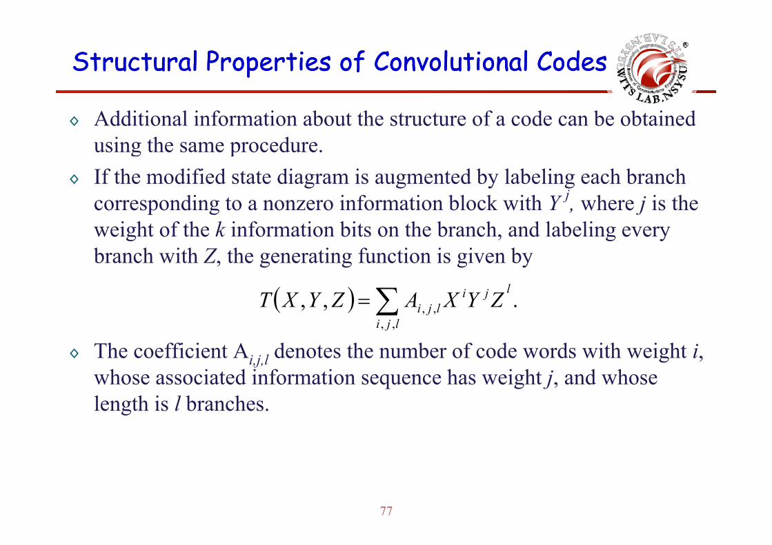
◊ Additional information about the structure of a code can be obtained using the same procedureusing the same procedure.
◊ If the modified state diagram is augmented by labeling each branch corresponding to a nonzero information block with Y j, where j is the p g , jweight of the k information bits on the branch, and labeling every branch with Z, the generating function is given by
( ) .,,,,
,,l
lji
jilji ZYXAZYXT ∑=
◊ The coefficient Ai,j,l denotes the number of code words with weight i,whose associated information sequence has weight j, and whose l h i l b hlength is l branches.
77

Structural Properties of Structural Properties of ConvolutionalConvolutional CodesCodes
The augment state diagram for the (2, 1, 3) codes.
78
Structural Properties of Structural Properties of ConvolutionalConvolutional CodesCodes
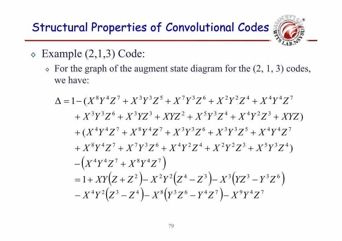
◊ Example (2,1,3) Code:F th h f th t t t di f th (2 1 3) d◊ For the graph of the augment state diagram for the (2, 1, 3) codes, we have:
324435233633
744422637533748
) (1Δ
XYZZYXZYXXYZYZXZYXZYXZYXZYXZYXZYX
++++++
++++−=
435322424637748
744533633748744
)(
)
ZYXZYXZYXZYXZYXZYXZYXZYXZYXZYX
+++++
+++++
( )( ) ( ) ( )633334222
748744
) ZYXZYX
ZYXZYXZYXZYXZYX+−
+++++
( ) ( ) ( )( ) ( ) 749746384324
633334222
1
ZYXZYZYXZZYXZYYZXZZYXZZXY
−−−−−
−−−−++=
79

Structural Properties of Structural Properties of ConvolutionalConvolutional CodesCodes
◊ Example (2,1,3) Code: (cont.)( ) ( )731126378412∑◊ ( ) ( )
( ) 8483222526
731126378412
1)1(
111
ZYXZYXZZXYZYX
XYZZYXXYZZYXZYXFi
ii
⋅+++−+
−+−+⋅=Δ∑( )
( ) ( )52847526
32447737 11 1)1(
ZYXYZXZYXZYXXYZYZXXYZZYXZYXZYXZZXYZYX
−−+−+
++++
◊ Hence the generating function is
52847526 ZYXYZXZYX −+=
◊ Hence the generating function is
( )Δ
−+=
52847526
,, ZYXYZXZYXZYXT
( )( )+++++
+++=Δ
948474628
736347526
2
ZYZYZYZYXZYZYYZXZYX
80
( )+++++ 2 ZYZYZYZYX
Structural Properties of Structural Properties of ConvolutionalConvolutional CodesCodes
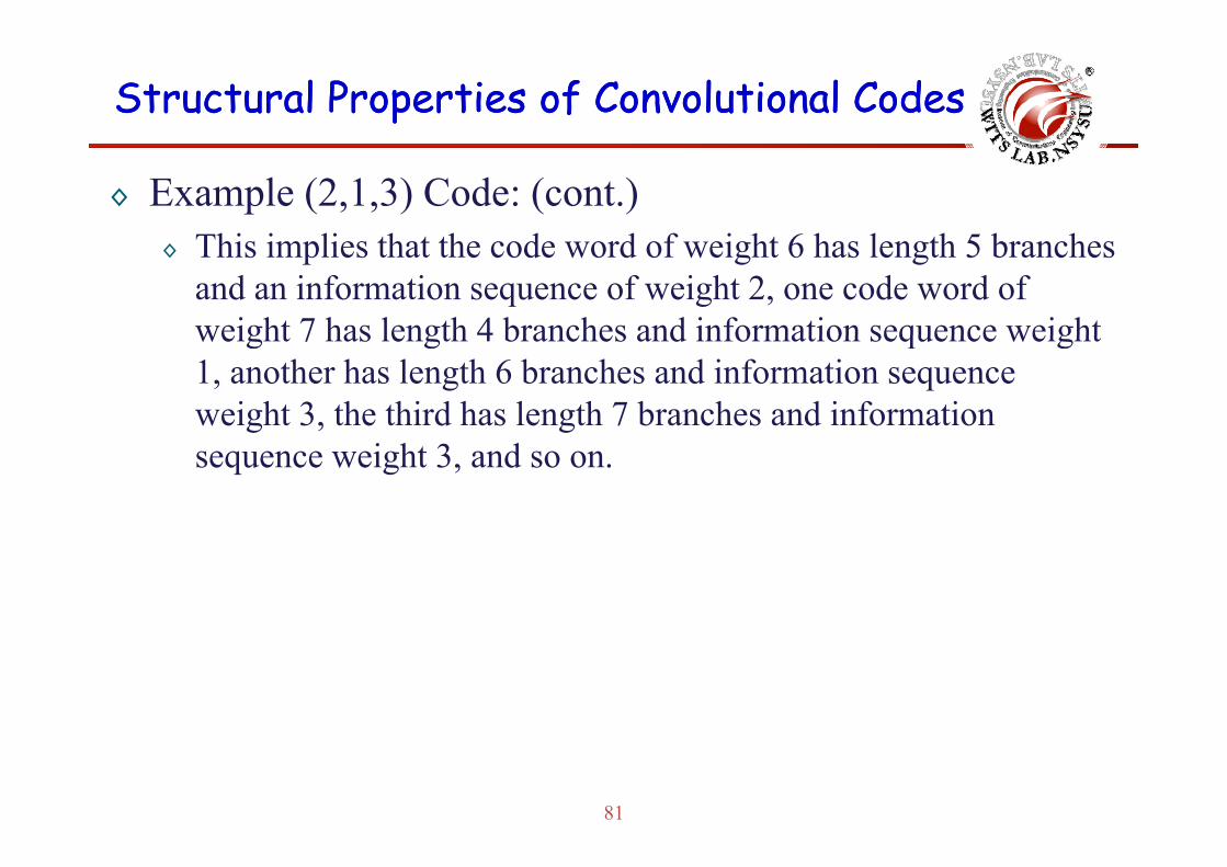
◊ Example (2,1,3) Code: (cont.)Thi i li th t th d d f i ht 6 h l th 5 b h◊ This implies that the code word of weight 6 has length 5 branches and an information sequence of weight 2, one code word of weight 7 has length 4 branches and information sequence weightweight 7 has length 4 branches and information sequence weight 1, another has length 6 branches and information sequence weight 3, the third has length 7 branches and information sequence weight 3, and so on.
81

The Transfer Function of a The Transfer Function of a ConvolutionalConvolutional CodeCode
◊ The state diagram can be used to obtain the distance propertyto obtain the distance property of a convolutional code.
◊ Without loss of generality, we g y,assume that the all-zero code sequence is the input to the encoder.
82

The Transfer Function of a The Transfer Function of a ConvolutionalConvolutional CodeCode
◊ First, we label the branches of the state diagram as either D0=1, D1, D2 or D3 where the exponent of D denotes the Hamming distanceD , or D , where the exponent of D denotes the Hamming distancebetween the sequence of output bits corresponding to each branch and the sequence of output bits corresponding to the all-zero branch.
◊ The self-loop at node a can be eliminated, since it contributes nothing to the distance properties of a code sequence relative to the all-zero code sequence.
◊ Furthermore, node a is split into two nodes, one of which represents th i t d th th th t t f th t t dithe input and the other the output of the state diagram.
83
The Transfer Function of a The Transfer Function of a ConvolutionalConvolutional CodeCode
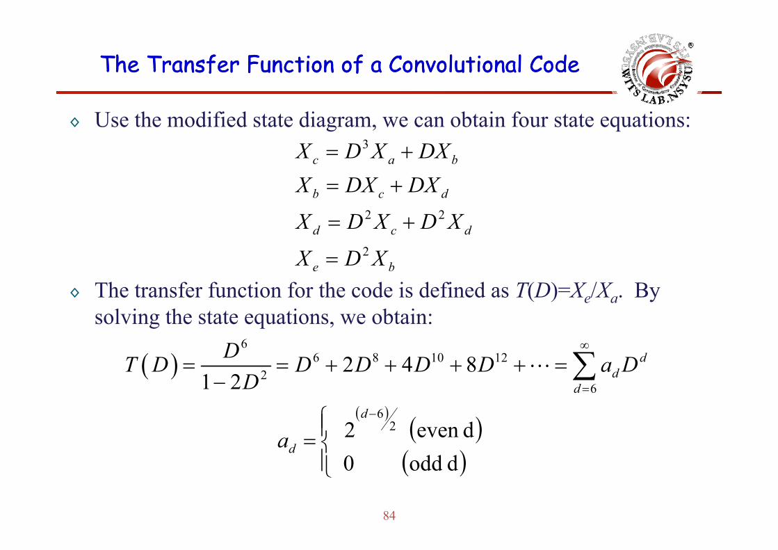
◊ Use the modified state diagram, we can obtain four state equations:3X D X DX= +
2 2
c a b
b c d
X D X DXX DX DX
= +
= +2 2
2
d c d
e b
X D X D X
X D X
= +
=◊ The transfer function for the code is defined as T(D)=Xe/Xa. By
solving the state equations, we obtain:
( )6
6 8 10 122
6
2 4 81 2
dd
d
DT D D D D D a DD
∞
=
= = + + + + =− ∑
( )( )( )⎪⎩
⎪⎨⎧
=−
dodd0 deven 2 2
6d
da
84
( )⎪⎩ d odd 0

The Transfer Function of a The Transfer Function of a ConvolutionalConvolutional CodeCode
◊ The transfer function can be used to provide more detailed information than just the distance of the various pathsinformation than just the distance of the various paths.
◊ Suppose we introduce a factor N into all branch transitions caused by the input bit 1.y p
◊ Furthermore, we introduce a factor of J into each branch of the state diagram so that the exponent of J will serve as a counting variable to g p gindicate the number of branches in any given path from node a to node e.
85
The Transfer Function of a The Transfer Function of a ConvolutionalConvolutional CodeCode
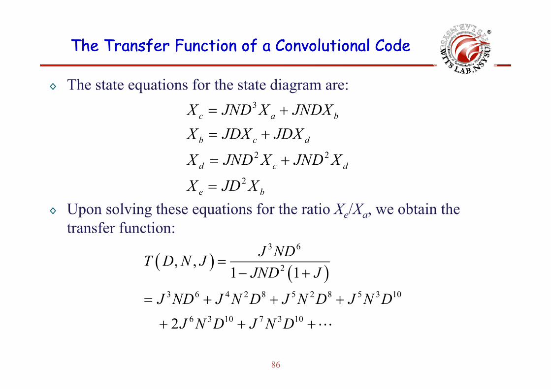
◊ The state equations for the state diagram are:3X JND X JNDX3
c a b
b c d
X JND X JNDXX JDX JDX
= += +
2 2
2d c d
e b
X JND X JND X
X JD X
= +
=◊ Upon solving these equations for the ratio Xe/Xa, we obtain the
transfer function:
e b
( ) ( )3 6
2, ,1 1
J NDT D N JJND J
=− +( )
3 6 4 2 8 5 2 8 5 3 10
6 3 10 7 3 102J ND J N D J N D J N D
J N D J N D= + + +
+ + +
86
2J N D J N D+ + +

The Transfer Function of a The Transfer Function of a ConvolutionalConvolutional CodeCode
◊ The exponent of the factor J indicates the length of the path that merges with the all-zero path for the first timemerges with the all zero path for the first time.
◊ The exponent of the factor N indicates the number of 1s in the information sequence for that path.q p
◊ The exponent of D indicates the distance of the sequence of encoded bits for that path from the all-zero sequence.p q
◊ Reference: John G. Proakis, “Digital Communications,” Fourth Edition, pp. , g , , pp477— 482, McGraw-Hill, 2001.
87
Structural Properties of Structural Properties of ConvolutionalConvolutional CodesCodes
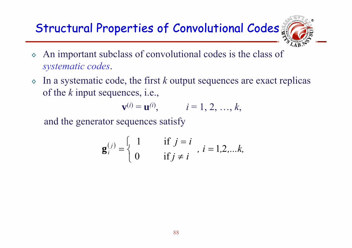
◊ An important subclass of convolutional codes is the class of systematic codessystematic codes.
◊ In a systematic code, the first k output sequences are exact replicas of the k input sequences, i.e.,p q , ,
v(i) = u(i), i = 1, 2, …, k,and the generator sequences satisfyand the generator sequences satisfy
( ) ,...k, , , ii j j
i 21if 1
=⎨⎧ =
=g , ,,,ij i if0⎩
⎨ ≠g
88
Structural Properties of Structural Properties of ConvolutionalConvolutional CodesCodes
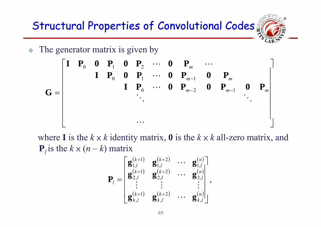
◊ The generator matrix is given by ⎤⎡ P0P0P0PI
⎥⎥⎥⎤
⎢⎢⎢⎡
− mm
m
P0P0P0PIP0P0P0PI
P0P0P0PI110
210
⎥⎥⎥⎥
⎢⎢⎢⎢= −− mmm P0P0P0PIG 120
where I is the k × k identity matrix 0 is the k × k all-zero matrix and
⎥⎦
⎢⎣
where I is the k × k identity matrix, 0 is the k × k all zero matrix, and Pl is the k × (n – k) matrix
( ) ( ) ( )1
21
11
⎥⎤
⎢⎡ ++ n
lkl
kl ggg
( ) ( ) ( ), ,2
2,2
1,2
,1,1,1
⎥⎥⎥⎥⎤
⎢⎢⎢⎢⎡
=++ n
lkl
kl
lll
lgggggg
P
89
( ) ( ) ( ),
2,
1,
⎥⎦⎢⎣++ n
lkk
lkk
lk ggg
Structural Properties of Structural Properties of ConvolutionalConvolutional CodesCodes
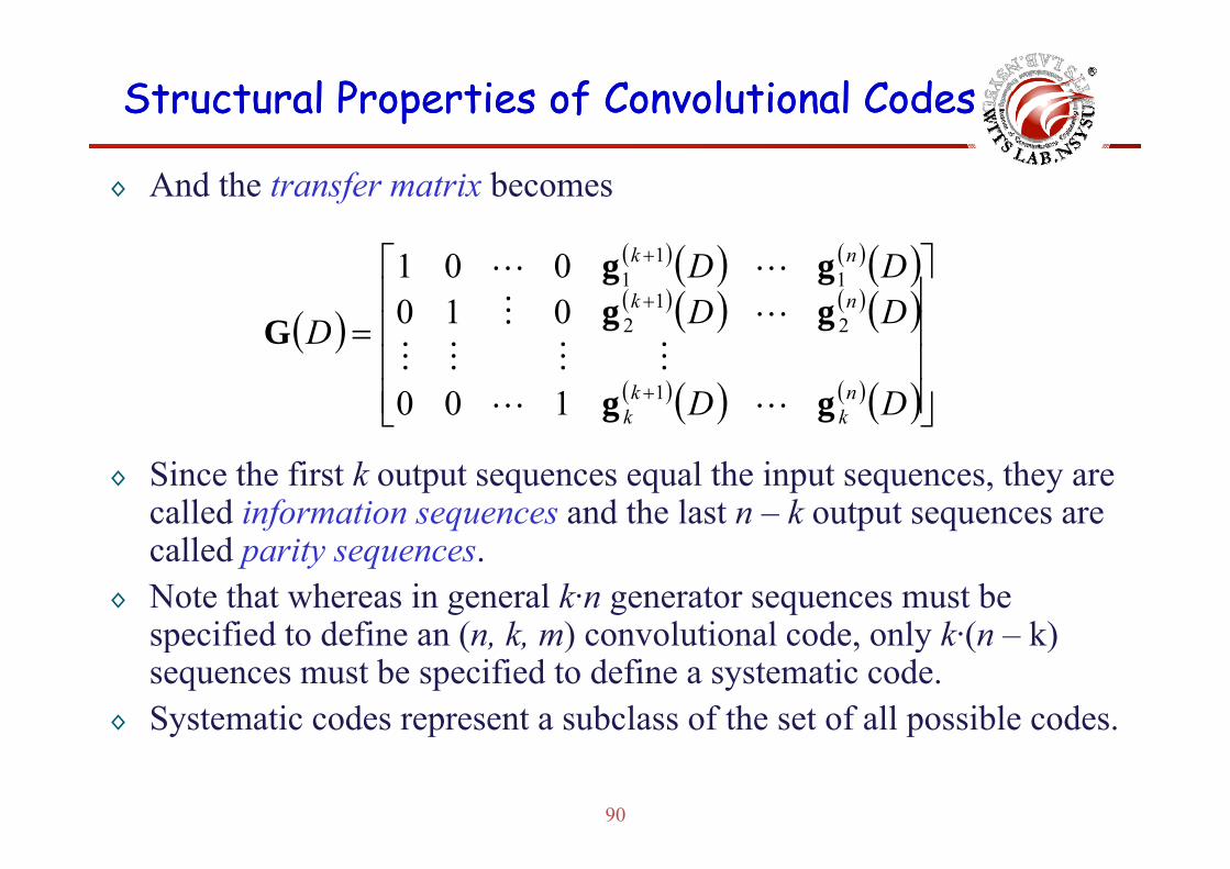
◊ And the transfer matrix becomes
( )
( ) ( ) ( ) ( )( ) ( ) ( ) ( )⎥
⎥⎤
⎢⎢⎡
=+
+
DDDD
Dnk
nk
gggg
G 21
2
11
1
010001
( )( ) ( ) ( ) ( )⎥
⎥⎥
⎦⎢⎢⎢
⎣
=
+ DD
Dn
kk
k gg
G1100
◊ Since the first k output sequences equal the input sequences, they are called information sequences and the last n – k output sequences are called parity sequences.
◊ Note that whereas in general k·n generator sequences must be specified to define an (n k m) convolutional code only k·(n k)specified to define an (n, k, m) convolutional code, only k·(n – k) sequences must be specified to define a systematic code.
◊ Systematic codes represent a subclass of the set of all possible codes.
90
y p p
Structural Properties of Structural Properties of ConvolutionalConvolutional CodesCodes
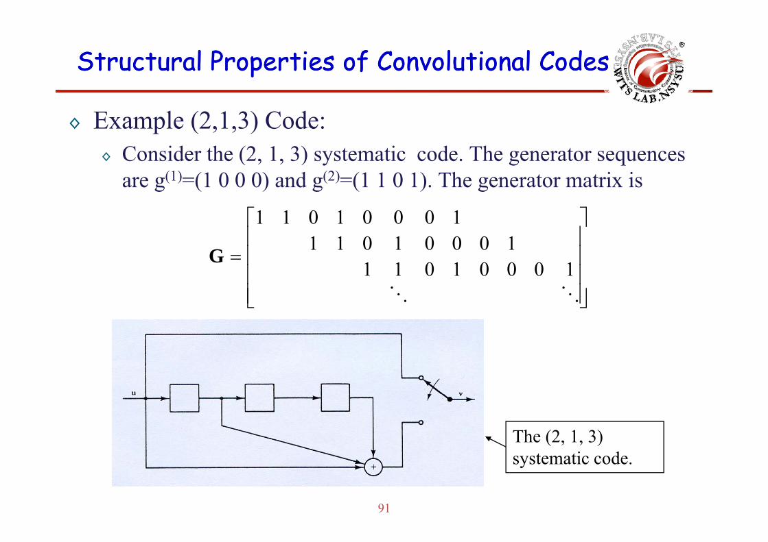
◊ Example (2,1,3) Code:C id th (2 1 3) t ti d Th t◊ Consider the (2, 1, 3) systematic code. The generator sequences are g(1)=(1 0 0 0) and g(2)=(1 1 0 1). The generator matrix is
⎤⎡
⎥⎥⎥⎤
⎢⎢⎢⎡
=10001011
1000101110001011
G
⎥⎥⎦⎢
⎢⎣
10001011
The (2, 1, 3) t ti d
91
systematic code.

Structural Properties of Structural Properties of ConvolutionalConvolutional CodesCodes
◊ Example (2,1,3) Code:Th t f f ti t i i g(1) (1 0 0 0) and g(2) (1 1 0 1)◊ The transfer function matrix is
G(D) = [1 1 + D + D3].
g(1)=(1 0 0 0) and g(2)=(1 1 0 1).
◊ For an input sequence u(D) = 1 + D2 + D3, the information sequence is
( ) ( ) ( ) ( ) ( ) ( ) 323211 111 DDDDDDD ++=⋅++== guv
and the parity sequence is
( ) ( ) ( ) ( ) ( ) ( )( )33222 11( ) ( ) ( ) ( ) ( ) ( )( )65432
33222
1 11DDDDDD
DDDDDDD++++++=
++++== guv
92
Structural Properties of Structural Properties of ConvolutionalConvolutional CodesCodes
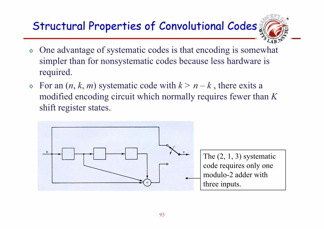
◊ One advantage of systematic codes is that encoding is somewhat simpler than for nonsystematic codes because less hardware issimpler than for nonsystematic codes because less hardware is required.
◊ For an (n, k, m) systematic code with k > n – k , there exits a ( , , ) y ,modified encoding circuit which normally requires fewer than Kshift register states.
The (2, 1, 3) systematic code requires only onecode requires only one modulo-2 adder with three inputs.
93
Structural Properties of Structural Properties of ConvolutionalConvolutional CodesCodes
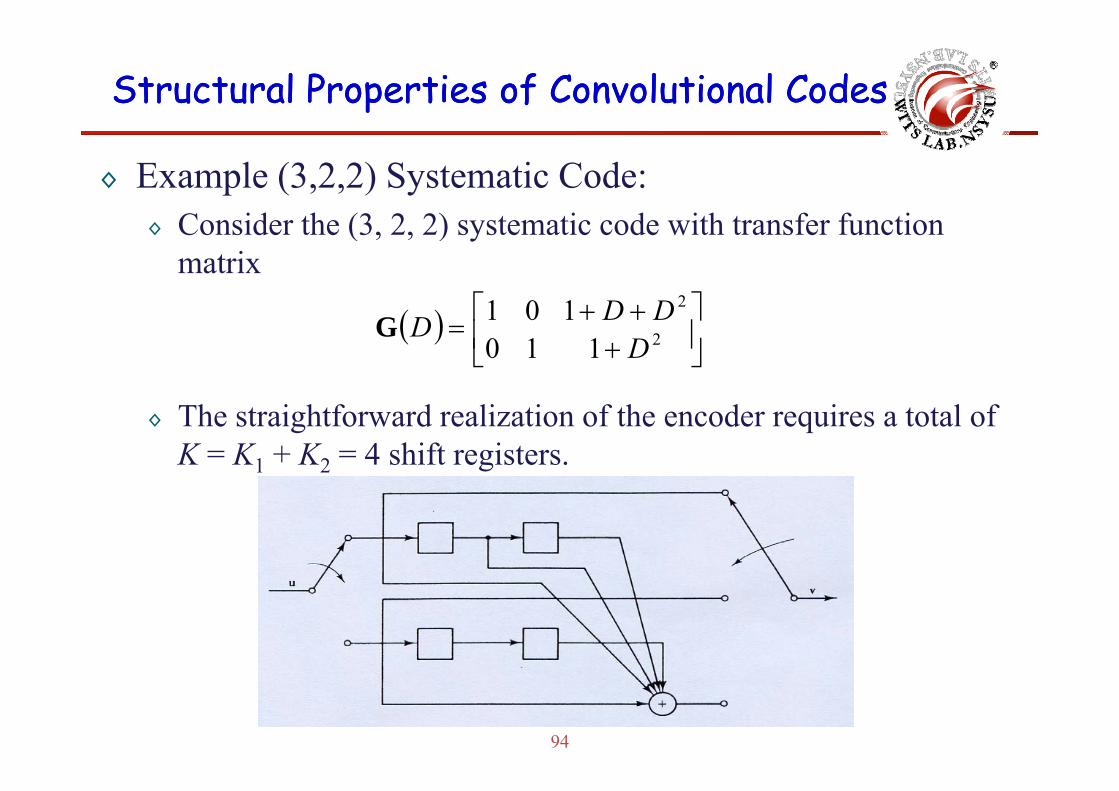
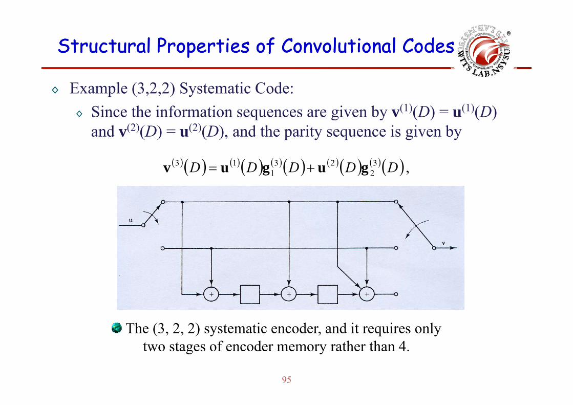
◊ Example (3,2,2) Systematic Code:C id th (3 2 2) t ti d ith t f f ti◊ Consider the (3, 2, 2) systematic code with transfer function matrix
⎤⎡ ++ 2101 DD( ) ⎥⎦
⎤⎢⎣
⎡+++= 2
2
110101
DDDDG
◊ The straightforward realization of the encoder requires a total of K = K1 + K2 = 4 shift registers.
94
Structural Properties of Structural Properties of ConvolutionalConvolutional CodesCodes
◊ Example (3,2,2) Systematic Code:◊ Since the information sequences are given by v(1)(D) = u(1)(D)◊ Since the information sequences are given by v(1)(D) = u(1)(D)
and v(2)(D) = u(2)(D), and the parity sequence is given by
( ) ( ) ( ) ( ) ( ) ( ) ( ) ( ) ( ) ( ) , 32
231
13 DDDDD guguv +=
The (3, 2, 2) systematic encoder, and it requires only
95
two stages of encoder memory rather than 4.
Structural Properties of Structural Properties of ConvolutionalConvolutional CodesCodes
◊ A complete discussion of the minimal encoder memory required to realize a convolutional code is given by Forneyrealize a convolutional code is given by Forney.
◊ In most cases the straightforward realization requiring K states of shift register memory is most efficient.g y
◊ In the case of an (n,k,m) systematic code with k>n-k, a simpler realization usually exists.y
◊ Another advantage of systematic codes is that no inverting circuit is needed for recovering the information sequence from the code word.
96

Structural Properties of Structural Properties of ConvolutionalConvolutional CodesCodes
◊ Nonsystematic codes, on the other hand, require an inverter to recover the information sequence; that is an n × k matrix G-1(D)recover the information sequence; that is, an n × k matrix G (D) must exit such that
G(D)G-1(D) = IDl( ) ( )for some l ≥ 0, where I is the k × k identity matrix.
◊ Since V(D) = U(D)G(D), we can obtain◊ Since V(D) U(D)G(D), we can obtainV(D)G-1(D) = U(D)G(D)G-1(D) = U(D)Dl ,
and the information sequence can be recovered with an l-time-unitand the information sequence can be recovered with an l time unit delay from the code word by letting V(D) be the input to the n-input, k-output linear sequential circuit whose transfer function matrix is G-1(D).
97

Structural Properties of Structural Properties of ConvolutionalConvolutional CodesCodes
◊ For an (n, 1, m) code, a transfer function matrix G(D) has a feedforward inverse G-1(D) of delay l if and only iffeedforward inverse G (D) of delay l if and only if
GCD[g(1)(D), g(2)(D),…, g(n)(D)] = Dl
for some l ≥ 0 where GCD denotes the greatest common divisorfor some l ≥ 0, where GCD denotes the greatest common divisor.◊ For an (n, k, m) code with k > 1,
be the determinants of the distinct k × k submatrices of thelet ( ), 1, 2, , ,i
nD i
k⎛ ⎞
Δ = ⎜ ⎟⎝ ⎠⎟
⎠⎞⎜
⎝⎛
knbe the determinants of the distinct k × k submatrices of the
transfer function matrix G(D).◊ A feedforward inverse of delay l exits if and only if
⎝ ⎠⎟⎠
⎜⎝k
◊ A feedforward inverse of delay l exits if and only if
li Dk
niD =⎥⎦⎤
⎢⎣⎡ ⎟
⎠⎞⎜
⎝⎛=Δ ,,2 ,1:)(GCD
for some l ≥ 0. k ⎥⎦⎢⎣ ⎠⎝
98

Structural Properties of Structural Properties of ConvolutionalConvolutional CodesCodes
◊ Example (2,1,3) Code:F th (2 1 3) d◊ For the (2, 1, 3) code,
d h f f i i
2 3 2 3 0GCD 1 , 1 1D D D D D D⎡ ⎤+ + + + + = =⎣ ⎦and the transfer function matrix
( )2
1 1 D DD− ⎡ ⎤+ +
= ⎢ ⎥G
provides the required inverse of delay 0 [i.e., G(D)G−1(D) = 1].
( ) 2D
D D⎢ ⎥+⎣ ⎦G
◊ The implementation of the inverse is shown below
99

Structural Properties of Structural Properties of ConvolutionalConvolutional CodesCodes
◊ Example (3,2,1) Code:F th (3 2 1) d th 2 2 b t i f G(D) i ld◊ For the (3, 2, 1) code , the 2 × 2 submatrices of G(D) yield determinants 1 + D + D2, 1 + D2, and 1. Since
2 21 1 1 1GCD D D D⎡ ⎤+ + +⎣ ⎦there exists a feedforward inverse of delay 0. Th i d t f f ti t i i
2 21 , 1 , 1 1GCD D D D⎡ ⎤+ + + =⎣ ⎦
◊ The required transfer function matrix is given by:
0 0⎡ ⎤⎢ ⎥( )1 1 11
D DD
− ⎢ ⎥= +⎢ ⎥⎢ ⎥⎣ ⎦
G
100
Structural Properties of Structural Properties of ConvolutionalConvolutional CodesCodes
◊ To understand what happens when a feedforward inverse does not exist, it is best to consider an example., p◊ For the (2, 1, 2) code with g(1)(D) = 1 + D and g(2)(D) = 1 + D2 ,
2GCD 1 1 1D D D⎡ ⎤+ + +⎣ ⎦
and a feedforward inverse does not exist.
GCD 1 , 1 1 ,D D D⎡ ⎤+ + = +⎣ ⎦
◊ If the information sequence is u(D) = 1/(1 + D) = 1 + D + D2
+ …, the output sequences are v(1)(D) = 1 and v(2)(D) = 1 + D; that is the code word contains only three nonzero bits eventhat is, the code word contains only three nonzero bits even though the information sequence has infinite weight.
◊ If this code word is transmitted over a BSC, and the three nonzero bits are changed to zeros by the channel noise, the received sequence will be all zeros.
101
Structural Properties of Structural Properties of ConvolutionalConvolutional CodesCodes
◊ A MLD will then produce the all-zero code word as its estimated, since this is a valid code word and it agrees exactly with thesince this is a valid code word and it agrees exactly with the received sequence.
◊ The estimated information sequence will be implying ( ) 0,D =uq p y gan infinite number of decoding errors caused by a finite number (only three in this case) of channel errors.
( ) 0,Du
◊ Clearly, this is a very undesirable circumstance, and the code is said to be subject to catastrophic error propagation, and is called
hi da catastrophic code.◊ and ( ) ( ) ( ) ( ) ( ) ( )1 2GCD , , , n lD D D D⎡ ⎤ =⎣ ⎦g g g… ( )GCD i DΔ⎡⎣
( )⎤for a code to be noncatastrophic.
( ): 1, 2,...., are necessary and sufficient conditions lni Dk⎤= =⎥⎦
102
for a code to be noncatastrophic.
Structural Properties of Structural Properties of ConvolutionalConvolutional CodesCodes
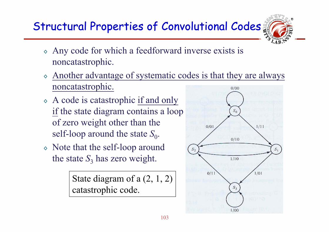
◊ Any code for which a feedforward inverse exists is noncatastrophicnoncatastrophic.
◊ Another advantage of systematic codes is that they are always noncatastrophic.p
◊ A code is catastrophic if and only if the state diagram contains a loop g pof zero weight other than the self-loop around the state S0.
◊ Note that the self-loop around the state S3 has zero weight.
State diagram of a (2, 1, 2) catastrophic code.
103

Structural Properties of Structural Properties of ConvolutionalConvolutional CodesCodes
◊ In choosing nonsystematic codes for use in a communication system it is important to avoid thecommunication system, it is important to avoid the selection of catastrophic codes.O l f i 1/(2 1) f ( 1 ) i d◊ Only a fraction 1/(2n − 1) of (n, 1, m) nonsystematic codes are catastrophic.
◊ A similar result for (n, k, m) codes with k > 1 is still lacking.
104

ConvolutionalConvolutional Decoder and Its Decoder and Its ConvolutionalConvolutional Decoder and Its Decoder and Its ApplicationsApplications
Wireless Information Transmission System Lab.Wireless Information Transmission System Lab.Institute of Communications EngineeringInstitute of Communications Engineeringg gg gNational Sun National Sun YatYat--sensen UniversityUniversity

IntroductionIntroduction
◊ In 1967, Viterbi introduced a decoding algorithm for convolutional codes which has since become known asconvolutional codes which has since become known as Viterbi algorithm.
O h d h h i bi l i h◊ Later, Omura showed that the Viterbi algorithm was equivalent to finding the shortest path through a weighted
hgraph.◊ Forney recognized that it was in fact a maximum
likelihood decoding algorithm for convolutional codes; that is, the decoder output selected is always the code word that gives the largest value of the log-likelihood function.
106
The The ViterbiViterbi AlgorithmAlgorithm
◊ In order to understand Viterbi’s decoding algorithm, it is convenient to expand the state diagram of the encoder in time (i e to representto expand the state diagram of the encoder in time (i.e., to represent each time unit with a separate state diagram).
◊ The resulting structure is called a trellis diagram, and is shown in g g ,Figure (a) for the (3, 1, 2) code with
( ) 2 21 , 1 , 1D D D D D⎡ ⎤= + + + +⎣ ⎦Gand an information sequence of length L=5.
◊ The trellis diagram contains L+m+1 time units or levels, and these
( ) ⎣ ⎦
g ,are labeled from 0 to L+m in Figure (a).
◊ Assuming that the encoder always starts in state S0 and returns to state S0, the first m time units correspond to the encoder’s departure from state S0, and the last m time units correspond to the encoder’s
t t t t S
107
return to state S0.
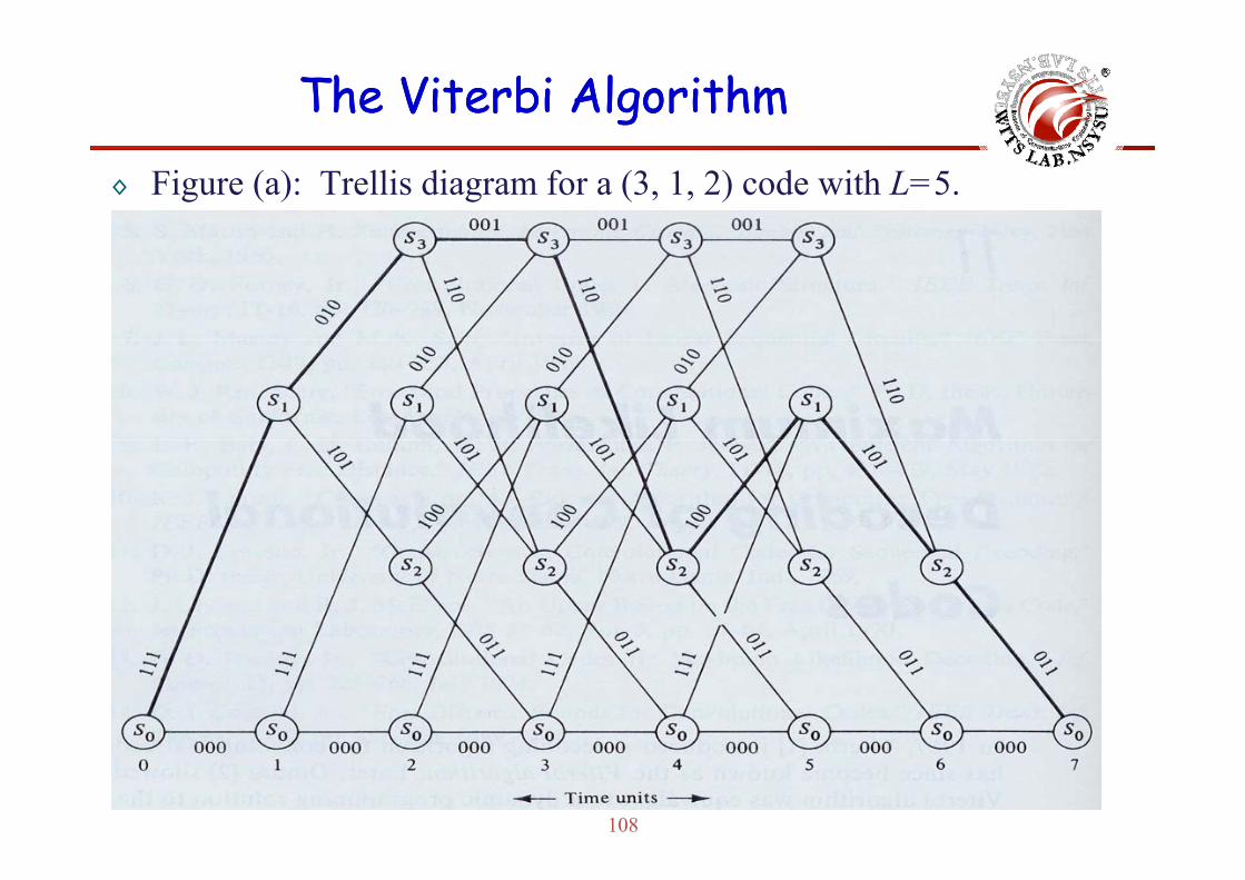
The The ViterbiViterbi AlgorithmAlgorithm◊ Figure (a): Trellis diagram for a (3, 1, 2) code with L=5.
108

The The ViterbiViterbi AlgorithmAlgorithm
◊ Not all states can be reached in the first m or the last m time units. However in the center portion of the trellis all states are possibleHowever, in the center portion of the trellis, all states are possible, and each time unit contains a replica of the state diagram.
◊ There are two branches leaving and entering each state.g g◊ The upper branch leaving each state at time unit i represents the
input ui = 1, while the lower branch represents ui = 0.p i p i
◊ Each branch is labeled with the n corresponding outputs vi, and each of the 2L code words of length N = n(L + m) is represented by a unique path through the trellis.
◊ For example, the code word corresponding to the information (1 1 1 0 1) i h hi hli h d i Fi ( )sequence u = (1 1 1 0 1) is shown highlighted in Figure (a).
109

The The ViterbiViterbi AlgorithmAlgorithm
◊ In the general case of an (n, k, m) code and an information sequence of length kL there are 2k branches leaving and entering each stateof length kL, there are 2 branches leaving and entering each state, and 2kL distinct paths through the trellis corresponding to the 2kL
code words.◊ Now assume that an information sequence u = (u0,…, uL−1) of
length kL is encoded into a code word v = (v0, v1,…, vL+m−1) of length N = n(L + m), and that a sequence r = (r0, r1,…, rL+m−1) is received over a discrete memoryless channel (DMC).Alt ti l th b itt ( )◊ Alternatively, these sequences can be written as u = (u0,…, ukL−1), v = (v0, v1,…, vN−1), r = (r0, r1,…, rN−1), where the subscripts now simply represent the ordering of the symbols in each sequencesimply represent the ordering of the symbols in each sequence.
110

The The ViterbiViterbi AlgorithmAlgorithm
◊ As a general rule of detection, the decoder must produce an estimate of the code word v based on the received sequence rv̂ of the code word v based on the received sequence r.
◊ A maximum likelihood decoder (MLD) for a DMC chooses as the code word v which maximizes the log-likelihood function
vv̂
logP(r |v).◊ Since for a DMC 1 1L m N+ − −
it follows that( ) ( ) ( )
0 0
| | | ,i i i ii i
P P P r v= =
= =∏ ∏r v r v
1 1L m N+
h P( | ) i h l t iti b bilit
( ) ( ) ( )1 1
0 0log | log | log | ------ (A)
L m N
i i i ii i
P P P r v+ − −
= =
= =∑ ∑r v r v
where P(ri |vi) is a channel transition probability.◊ This is a minimum error probability decoding rule when all code
words are equally likely
111
words are equally likely.

The The ViterbiViterbi AlgorithmAlgorithm
◊ The log-likelihood function log P(r |v) is called the metric associated with the path v and is denoted M(r |v)with the path v, and is denoted M(r |v).
◊ The terms log P(ri |vi) in the sum of Equation (A) are called branch metrics, and are denoted M(ri |vi), whereas the terms log P(ri |vi) are , ( i | i), g ( i | i)called bit metrics, and are denoted M(ri |vi).
◊ The path metric M(r |v) can be written asp ( | )
( ) ( ) ( )1 1
0 0| | | .
L m N
i i i ii i
M M M r v+ − −
= =
= =∑ ∑r v r v
◊ The decision made by the log-likelihood function is called the soft-decision.If h h l i dd d i h AWGN f d i i d di l d◊ If the channel is added with AWGN, soft-decision decoding leads to finding the path with minimum Euclidean distance.
112

The The ViterbiViterbi AlgorithmAlgorithm
◊ A partial path metric for the first j branches of a path can now be expressed asexpressed as
[ ]( ) ( )1
0| | .
j
i iji
M M−
= ∑r v r v
◊ The following algorithm, when applied to the received sequence rfrom a DMC, finds the path through the trellis with the largest
0i=
from a DMC, finds the path through the trellis with the largest metric (i.e., the maximum likelihood path).
◊ The algorithm processes r in an iterative manner.g p◊ At each step, it compares the metrics of all paths entering each state,
and stores the path with the largest metric, called the survivor, together with its metric.
113
The The ViterbiViterbi AlgorithmAlgorithm
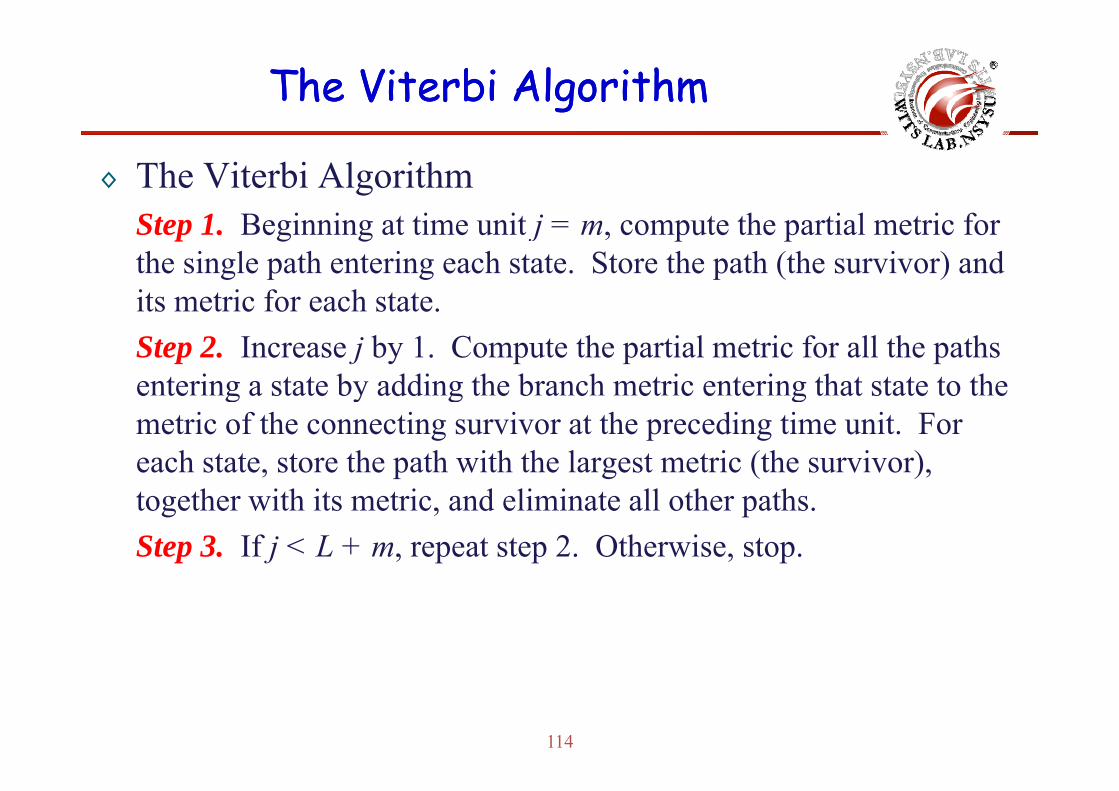
◊ The Viterbi AlgorithmS 1 B i i t ti it j t th ti l t i fStep 1. Beginning at time unit j = m, compute the partial metric for the single path entering each state. Store the path (the survivor) and its metric for each stateits metric for each state.Step 2. Increase j by 1. Compute the partial metric for all the paths entering a state by adding the branch metric entering that state to the e te g a state by add g t e b a c et c e te g t at state to t emetric of the connecting survivor at the preceding time unit. For each state, store the path with the largest metric (the survivor), together with its metric, and eliminate all other paths.Step 3. If j < L + m, repeat step 2. Otherwise, stop.
114

The The ViterbiViterbi AlgorithmAlgorithm
◊ There are 2K survivors from time unit m through time unit L, one for each of the 2K states (K is the total number of registers)each of the 2 states. (K is the total number of registers)
◊ After time unit L there are fewer survivors, since there are fewer states while the encoder is returning to the all-zero state.g
◊ Finally, at time unit L + m, there is only one state, the all-zero state, and hence only one survivor, and the algorithm terminates.y g
◊ Theorem The final survivor in the Viterbi algorithm is maximum likelihood path, that is,
v
( ) ( )| | , all .M M≥ ≠r v r v v v
115

The The ViterbiViterbi AlgorithmAlgorithm
◊ Proof.◊ Assume that the maximum likelihood path is◊ Assume that the maximum likelihood path is
eliminated by the algorithm at time unit j, as illustrated in figure.g
◊ This implies that the partial path metric of thesurvivor exceeds that of the maximum likelihood path at this point.
◊ If the remaining portion of the maximum likelihood path is appended onto the survivorat time unit j, the total metric of this pathwill exceed the total metric of thewill exceed the total metric of the maximum likelihood path.
116

The The ViterbiViterbi AlgorithmAlgorithm
◊ But this contradicts the definition of the maximum likelihood path as the path with the largest metric Hence the maximumpath as the path with the largest metric. Hence, the maximum likelihood path cannot be eliminated by the algorithm, and must be the final survivor.
◊ Therefore, the Viterbi algorithm is optimum in the sense that it always finds the maximum likelihood path through the trellis.
◊ In the special case of a binary symmetric channel (BSC) with transition probability p < ½, the received sequence r is binary (Q = 2)
d th l lik lih d f ti b (E 1 11)and the log-likelihood function becomes (Eq 1.11):
( ) ( ) ( )log | , log log 1pP d N p= + −r v r v
where d(r, v) is the Hamming distance between r and v.
( ) ( ) ( )g | , g g1
pp−
117
The The ViterbiViterbi AlgorithmAlgorithm
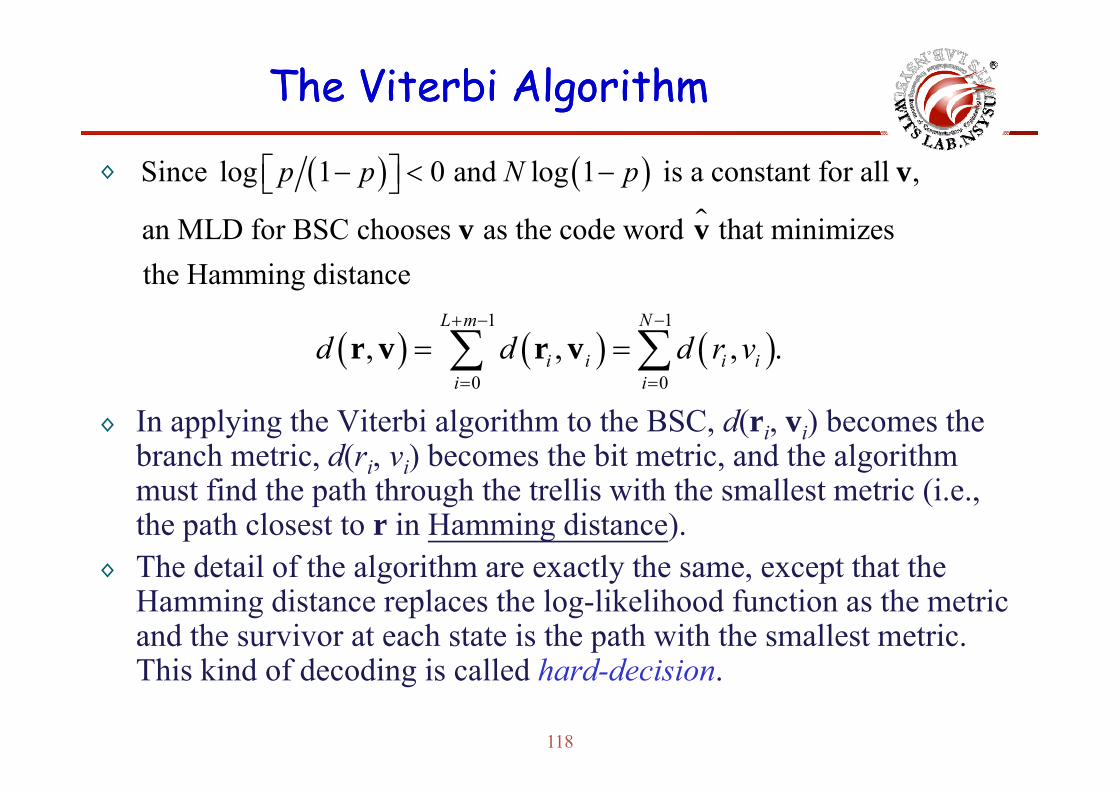
◊ ( ) ( )Since log 1 0 and log 1 is a constant for all , p p N p− < −⎡ ⎤⎣ ⎦ v
an MLD for BSC chooses as the code word that minimizes the Hamming distance
v v
( ) ( ) ( )1 1
0 0, , , .
L m N
i i i ii i
d d d r v+ − −
= =
= =∑ ∑r v r v
◊ In applying the Viterbi algorithm to the BSC, d(ri, vi) becomes the branch metric, d(ri, vi) becomes the bit metric, and the algorithm
t fi d th th th h th t lli ith th ll t t i (imust find the path through the trellis with the smallest metric (i.e., the path closest to r in Hamming distance).
◊ The detail of the algorithm are exactly the same, except that the◊ The detail of the algorithm are exactly the same, except that the Hamming distance replaces the log-likelihood function as the metric and the survivor at each state is the path with the smallest metric. Thi ki d f d di i ll d h d d i i
118
This kind of decoding is called hard-decision.

The The ViterbiViterbi AlgorithmAlgorithm◊ Example 11.2:
◊ The application of the Viterbi algorithm to a BSC is shown in the◊ The application of the Viterbi algorithm to a BSC is shown in the following figure. Assume that a code word from the trellis diagram of the (3, 1, 2) code of Figure (a) is transmitted over a BSC and that the received sequence is
( )1 1 0, 1 1 0, 1 1 0, 1 1 1, 0 1 0, 1 0 1, 1 0 1 .=r
119

The The ViterbiViterbi AlgorithmAlgorithm◊ Example 11.2 (cont.):
◊ The final survivor◊ The final survivor
is shown as the highlighted path in the figure and the decoded( )1 1 1, 0 1 0, 1 1 0, 0 1 1, 1 1 1, 1 0 1, 0 1 1=v
is shown as the highlighted path in the figure, and the decoded information sequence is
◊ The fact that the final survivor has a metric of 7 means that no( )1 1 0 0 1 .=u
◊ The fact that the final survivor has a metric of 7 means that no other path through the trellis differs from r in fewer than seven positions.
◊ Note that at some states neither path is crossed out. This indicates a tie in the metric values of the two paths entering that state.
◊ If the final survivor goes through any of these states, there is more than one ma im m likelihood path (i e more than one path
120
more than one maximum likelihood path (i.e., more than one path whose distance from r is minimum).

The The ViterbiViterbi AlgorithmAlgorithm
◊ Example 11.2 (cont.):F i l t ti i t f i h ti i t i◊ From an implementation point of view, whenever a tie in metric values occurs, one path is arbitrarily selected as the survivor, because of the impracticality of storing a variable number ofbecause of the impracticality of storing a variable number of paths.
◊ This arbitrary resolution of ties has no effect on the decoding ◊ s a b t a y eso ut o o t es as o e ect o t e decod gerror probability.
121

Punctured Punctured ConvolutionalConvolutional CodesCodes
◊ In some practical applications, there is a need to employ high-rate convolutional codes e g rate of (n-1)/nconvolutional codes, e.g. rate of (n 1)/n.
◊ The trellis for such high-rate codes has 2n-1 branches that enter each state. Consequently, there are 2n-1 metric computations per state that q y, p pmust be performed in implementing the Viterbi algorithm and as many comparisons of the updated metrics in order to select the best path at each state.
◊ The computational complexity inherent in the implementation of the d d f hi h t l ti l d b id d bdecoder of a high-rate convolutional code can be avoided by designing the high-rate code from a low-rate code in which some of the coded bits are deleted (punctured) from transmissionthe coded bits are deleted (punctured) from transmission.
◊ Puncturing a code reduces the free distance.
122
Punctured Punctured ConvolutionalConvolutional CodesCodes
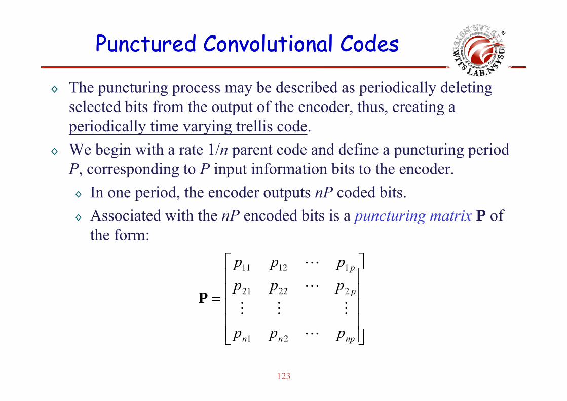
◊ The puncturing process may be described as periodically deleting selected bits from the output of the encoder thus creating aselected bits from the output of the encoder, thus, creating a periodically time varying trellis code.
◊ We begin with a rate 1/n parent code and define a puncturing period g p p g pP, corresponding to P input information bits to the encoder.◊ In one period, the encoder outputs nP coded bits.p p◊ Associated with the nP encoded bits is a puncturing matrix P of
the form:
⎥⎥⎤
⎢⎢⎡
p
p
pppppp
22221
11211
⎥⎥⎥⎥
⎦⎢⎢⎢⎢
⎣
= p
ppp
ppp
21
22221P
123
⎥⎦⎢⎣ npnn ppp 21

Punctured Punctured ConvolutionalConvolutional CodesCodes
◊ Each column of P corresponds to the n possible output bits from the encoder for each input bit and each element of P is either 0 or 1encoder for each input bit and each element of P is either 0 or 1.◊ When pij=1, the corresponding output bit from the encoder is
transmitted.◊ When pij=0, the corresponding output bit from the encoder is
deleted.◊ The code rate is determined by the period P and the number of
bits deleted.◊ If we delete N bits out of nP, the code rate is P/(nP-N).
124

Punctured Punctured ConvolutionalConvolutional CodesCodes
◊ Example: Constructing a rate ¾ code by puncturing the output of the rate 1/3 K=3 encoder as shown in the following figurerate 1/3, K 3 encoder as shown in the following figure.
◊ There are many choices for P and M to achieve the desired rate. We may take the smallest value of P, namely, P=3.y , y,
◊ Out of every nP=9 output bits, we delete N=5 bits.
OriginalCircuit.
125

Punctured Punctured ConvolutionalConvolutional CodesCodes
◊ Example: Trellis of a rate ¾ convolutional code by puncturing the output of the rate 1/3 K=3 encoderoutput of the rate 1/3, K 3 encoder .
126
Punctured Punctured ConvolutionalConvolutional CodesCodes
◊ Some puncturing matrices are better than others in that the trellis paths have better Hamming distance propertiespaths have better Hamming distance properties.
◊ A computer search is usually employed to find good puncturing matrices.
◊ Generally, the high-rate punctured convolutional codes generated in this manner have a free distance that is either equal to or 1 bit lessqthan the best same high-rate convolutional code obtained directly without puncturing.
◊ In general, high-rate codes with good distance properties are obtained by puncturing rate ½ maximum free distance codes.
127

Punctured Punctured ConvolutionalConvolutional CodesCodes
128

Punctured Punctured ConvolutionalConvolutional CodesCodes
◊ The decoding of punctured convolutional codes is performed in the same manner as the decoding of the low-rate 1/n parent code usingsame manner as the decoding of the low rate 1/n parent code, using the trellis of the 1/n code.
◊ When one or more bits in a branch are punctured, the corresponding p , p gbranch metric increment is computed based on the non-punctured bits, thus, the punctured bits do not contribute to the branch metrics.
◊ Error events in a punctured code are generally longer than error events in the low rate 1/n parent code.
◊ Consequently, the decoder must wait longer than five constraint lengths before making final decisions on the received bits.
129

RateRate--compatible Punctured compatible Punctured ConvolutionalConvolutional CodesCodes
◊ In the transmission of compressed digital speech signals and in some other applications there is a need to transmit some groups ofother applications, there is a need to transmit some groups of information bits with more redundancy than others.
◊ In other words, the different groups of information bits require , g p qunequal error protection to be provided in the transmission of the information sequence, where the more important bits are transmitted with more redundancy.
◊ Instead of using separate codes to encode the different groups of bits, it i d i bl t i l d th t h i bl d d Thiit is desirable to use a single code that has variable redundancy. This can be accomplished by puncturing the same low rate 1/nconvolutional code by different amounts as described by Hagenauerconvolutional code by different amounts as described by Hagenauer(1988).
130

RateRate--compatible Punctured compatible Punctured ConvolutionalConvolutional CodesCodes
◊ The puncturing matrices are selected to satisfy a rate- compatibility criterion where the basic requirement is that lower-rate codescriterion, where the basic requirement is that lower rate codes (higher redundancy) should transmit the same coded bits as all higher-rate codes plus additional bits.
◊ The resulting codes obtained from a single rate 1/n convolutionalcode are called rate-compatible punctured convolutional (RCPC)code.
◊ In applying RCPC codes to systems that require unequal error t ti f th i f ti f t th fprotection of the information sequence, we may format the groups of
bits into a frame structure and each frame is terminated after the last group of information bits by K-1 zerosgroup of information bits by K 1 zeros.
131

RateRate--compatible Punctured compatible Punctured ConvolutionalConvolutional CodesCodes
◊ Example: Constructing a RCPC code from a rate 1/3RCPC code from a rate 1/3, K=4 maximum free distance convolutional code.◊ Note that when a 1 appears
in a puncturing matrix of a high-rate code, a 1 also appears in the same position for all lower rateposition for all lower-rate codes.
132

Practical ConsiderationsPractical Considerations
◊ The minimum free distance dfree can be freeincreased either by decreasing the code rateor by increasing theor by increasing the constraint length, or both.
◊ If hard-decision ◊ a d dec s odecoding is used, the performances (coding gains) are reduced bygains) are reduced by approximately 2 dB for the AWGN channel when compared with the soft-decision decoding.
133
Practical ConsiderationsPractical Considerations
◊ Two important issues in the implementation of Viterbi decoding are:◊ The effect of path memory truncation which is a desirable◊ The effect of path memory truncation, which is a desirable
feature that ensures a fixed decoding delay.◊ The degree of quantization of the input signal to the Viterbi◊ The degree of quantization of the input signal to the Viterbi
decoder.◊ The path memory truncation to about five constraint lengths has◊ The path memory truncation to about five constraint lengths has
been found to result in negligible performance loss.
134

Practical ConsiderationsPractical Considerations
◊ Bit error probability for rate ½ Viterbi decodingrate ½ Viterbi decoding with eight-level quantized inputs to the decoder and 32-bit path memory.
135

Practical ConsiderationsPractical Considerations
◊ Performance of rate ½ codes with hard-codes with hard-decision Viterbi decoding and 32-bit gpath memory truncation
136

Practical ConsiderationsPractical Considerations
◊ Performance of rate ½, K=5 code with eight- four- andcode with eight-, four-, and two-level quantization at the input to the Viterbi pdecoder. Path truncation length=32 bits.
137

Practical ConsiderationsPractical Considerations
◊ Performance of rate ½, K=5 code with 32- 16-K 5 code with 32 , 16 , and 8-biy path memory truncation and eight- and two-level quantization.
138