convex optimization in signal processing and … · contents list of contributors page iv part i 1...

Convex Optimization in SignalProcessing and Communications

March 24, 2009

i

Contents

List of contributors page iv

Part I 1

1 Convex Analysis for Non-negative Blind Source Separation with Applica-

tion in Imaging 31.1 Introduction 31.2 Problem Statement 6

1.2.1 Assumptions 91.3 Review of Some Concepts in Convex Analysis 11

1.3.1 Affine Hull 111.3.2 Convex Hull 12

1.4 Non-negative Blind Source Separation Criterion via CAMNS 131.4.1 Convex Analysis of the Problem, and the CAMNS Criterion 131.4.2 An Alternative Form of the CAMNS Criterion 17

1.5 Systematic Linear Programming Method for CAMNS 201.6 Alternating Volume Maximization Heuristics for CAMNS 231.7 Numerical Results 27

1.7.1 Example of 3-Source Case: Cell Separation 281.7.2 Example of 4-Source Case: Ghosting Effect 291.7.3 Example of 5-Source Case: Human Face Separation 311.7.4 Monte Carlo Simulation: Noisy Environment 31

1.8 Summary and Discussion 341.9 Appendix 36

1.9.1 Proof of Lemma 1.2 361.9.2 Proof of Proposition 1.1 361.9.3 Proof of Lemma 1.5 371.9.4 Proof of Lemma 1.6 381.9.5 Proof of Lemma 1.7 381.9.6 Proof of Theorem 1.3 39

References 41Index 44

iii

List of contributors

Wing-Kin Ma

Wing-Kin Ma received the B.Eng. (with First Class Honors) in electrical andelectronic engineering from the University of Portsmouth, Portsmouth, U.K., in1995, and the M.Phil. and Ph.D. degrees, both in electronic engineering, fromthe Chinese University of Hong Kong (CUHK), Hong Kong, in 1997 and 2001,respectively.He is currently an Assistant Professor in the Department of Electronic Engineer-ing, CUHK. He was with the Institute of Communications Engineering, NationalTsing Hua University, Taiwan, also as an Assistant Professor, from 2005 to 2007.He is still holding an adjunct position there. Prior to becoming a faculty, he heldvarious research positions at McMaster University, Canada, CUHK, Hong Kong,and the University of Melbourne, Australia. His research interests are in signalprocessing and communications, with a recent emphasis on MIMO techniquesand convex optimization.Dr. Ma’s Ph.D. dissertation was commended to be “of very high quality and welldeserved honorary mentioning” by the Faculty of Engineering, CUHK, in 2001.He is currently an Associate Editor of the IEEE Transactions on Signal

Processing.

Tsung-Han Chan

Tsung-Han Chan received the B.S. degree from the Department of ElectricalEngineering, Yuan Ze University, Taoyuan, Taiwan, R.O.C., in 2004. He is cur-rently working towards the Ph.D. degree in the Institute of CommunicationsEngineering, National Tsing Hua University, Hsinchu, Taiwan, R.O.C. In 2008,he was a visiting Doctoral Graduate Research Assistant at Virginia Polytech-nic Institute and State University, Arlington. His research interests are in signalprocessing, convex optimization, and pattern analysis with a recent emphasis ondynamic medical imaging and remote sensing applications.

Chong-Yung Chi

Chong-Yung Chi received the Ph.D. degree in Electrical Engineering from theUniversity of Southern California in 1983. From 1983 to 1988, he was with the JetPropulsion Laboratory, Pasadena, California. He has been a Professor with theDepartment of Electrical Engineering since 1989 and the Institute of Communi-

iv

List of contributors v

cations Engineering (ICE) since 1999 (also the Chairman of ICE for 2002-2005),National Tsing Hua University, Hsinchu, Taiwan. He co-authored a technicalbook, Blind Equalization and System Identification, published by Springer 2006,and published more than 150 technical (journal and conference) papers. Hiscurrent research interests include signal processing for wireless communications,convex analysis and optimization for blind source separation, biomedical imagingand hyperspectral imaging.Dr. Chi is a senior member of IEEE. He has been a Technical Program Commit-tee member for many IEEE sponsored and co-sponsored workshops, symposiumsand conferences on signal processing and wireless communications, includingCo-organizer and general Co-chairman of IEEE SPAWC 2001, and Co-Chair ofSignal Processing for Communications Symposium, ChinaCOM 2008 & Chi-naCOM 2009. He was an Associate Editor for IEEE Trans. Signal Process-ing (5/2001∼4/2006), IEEE Trans. Circuits and Systems II (1/2006∼12/2007),and a member of Editorial Board of EURASIP Signal Processing Journal(6/2005∼5/2008), and an editor (7/2003∼12/2005) as well as a Guest Editor(2006) for EURASIP Journal on Applied Signal Processing. Currently, he is anAssociate Editor for IEEE Signal Processing Letters and IEEE Trans. Circuitsand Systems I, and a member of IEEE Signal Processing Committee on SignalProcessing Theory and Methods.

Yue Wang

Yue Wang received his B.S. and M.S. degrees in electrical and computer engi-neering from Shanghai Jiao Tong University in 1984 and 1987 respectively. Hereceived his Ph.D. degree in electrical engineering from University of MarylandGraduate School in 1995. In 1996, he was a postdoctoral fellow at GeorgetownUniversity School of Medicine. From 1996 to 2003, he was an assistant and laterassociate professor of electrical engineering at The Catholic University of Amer-ica. In 2003, he joined Virginia Polytechnic Institute and State University andis currently a full professor of electrical, computer, and biomedical engineering.Yue Wang became an elected Fellow of The American Institute for Medical andBiological Engineering (AIMBE) and ISI Highly Cited Researcher by ThomsonScientific in 2004. His research interests focus on statistical pattern recognition,machine learning, signal and image processing, with applications to computa-tional bioinformatics and biomedical imaging.

Part I

1

1 Convex Analysis for Non-negativeBlind Source Separation withApplication in Imaging

Wing-Kin Ma, Tsung-Han Chan, Chong-Yung Chi, and Yue Wang

Wing-Kin Ma is with the Chinese University of Hong Kong, Shatin, N.T., Hong Kong.Tsung-Han Chan is with the National Tsing Hua University, Hsinchu, Taiwan.Chong-Yung Chi is with the National Tsing Hua University, Hsinchu, Taiwan.Yue Wang is with the Virginia Polytechnic Institute and State University, Arlington, VA, USA.

In recent years, there has been a growing interest in blind separation of non-negative sources, as simply non-negative blind source separation (nBSS). Poten-tial applications of nBSS include biomedical imaging, multi/hyper-spectral imag-ing, and analytical chemistry. In this chapter, we describe a rather new endeavorof nBSS, where convex geometry is utilized to analyze the nBSS problem. Calledconvex analysis of mixtures of non-negative sources (CAMNS), the frameworkdescribed here makes use of a very special assumption called local dominance,which is a reasonable assumption for source signals exhibiting sparsity or highcontrast. Under the local dominant and some usual nBSS assumptions, we showthat the source signals can be perfectly identified by finding the extreme points ofan observation-constructed polyhedral set. Two methods for practically locatingthe extreme points are also derived. One is analysis-based with some appealingtheoretical guarantees, while the other is heuristic in comparison but is intu-itively expected to provide better robustness against model mismatches. Bothare based on linear programming and thus can be effectively implemented. Sim-ulation results on several data sets are presented to demonstrate the efficacy ofthe CAMNS-based methods over several other reported nBSS methods.

1.1 Introduction

Blind source separation (BSS) is a signal processing technique the purpose ofwhich is to separate source signals from observations, without information ofhow the source signals are mixed in the observations. BSS presents a technicallyvery challenging topic to the signal processing community, but it has stimulatedsignificant interest for many years due to its relevance to a wide variety of appli-cations. BSS has been applied to wireless communications and speech processing,and recently there has been an increasing interest in imaging applications.

3

4 Chapter 1. Convex Analysis for Non-negative Blind Source Separation with Application in Imaging

BSS methods are ‘blind’ in the sense that the mixing process is not known,at least not explicitly. But what is universally true for all BSS frameworks isthat we make certain presumptions on the source characteristics (and some-times on the mixing characteristics as well), and then exploit such characteris-tics during the blind separation process. For instance, independent componentanalysis (ICA) [1, 2], a major and very representative BSS framework on whichmany BSS methods are based, assumes that the sources are mutually uncorre-lated/independent random processes possibly with non-Gaussian distributions.There are many other possibilities one can consider; for example, using quasi-stationarity [3, 4] (speech signals are quasi-stationary), and using boundness ofthe source magnitudes [5, 6, 7] (suitable for digital signals). In choosing a rightBSS method for a particular application, it is important to examine whether theunderlying assumptions of the BSS method are a good match to the application.For instance, statistical independence is a reasonable assumption in applicationssuch as speech signal separation, but it may be violated in certain imaging sce-narios such as hyperspectral imaging [8].

This book chapter focuses on non-negative blind source separation (nBSS), inwhich the source signals are assumed to take on non-negative values. Naturally,images are non-negative signals. Potential applications of nBSS include biomed-ical imaging [9], hyperspectral imaging [10], and analytical chemistry [11]. Inbiomedical imaging, for instance, there are realistic, meaningful problems wherenBSS may serve as a powerful image analysis tool for practitioners. Such exam-ples will be briefly described in this book chapter.

In nBSS, how to cleverly utilize source non-negativity to achieve clean sepa-ration has been an intriguing subject that has received much attention recently.Presently available nBSS methods may be classified into two groups. One groupis similar to ICA: Assume that the sources are mutually uncorrelated or indepen-dent, but with non-negative source distributions. Methods falling in this classinclude non-negative ICA (nICA) [12], stochastic non-negative ICA (SNICA)[13], and Bayesian positive source separation (BPSS) [14]. In particular, in nICAthe blind separation criterion can theoretically guarantee perfect separation ofsources [15], under an additional assumption where the source distributions arenon-vanishing around zero (this is called the well-grounded condition).

Another group of nBSS methods does not rely on statistical assumptions.Roughly speaking, these methods explicitly exploit source non-negativity or evenmixing matrix non-negativity, with an attempt to achieve some kind of leastsquare fitting criterion. Methods falling in this group are generally known as (ormay be vaguely recognized as) non-negative matrix factorization (NMF) [16, 17].An advantage with NMF is that it does not operate on the premise of mutualuncorrelatedness/independence as in the first group of nBSS methods. NMF is anonconvex constrained optimization problem. A popular way of handling NMFis to apply gradient descent [17], but it is known to be suboptimal and slowlyconvergent. A projected quasi-Newton method has been incorporated in NMFto speed up its convergence [18]. Alternatively, alternating least squares (ALS)

Convex Analysis for Non-negative Blind Source Separation with Application in Imaging 5

[19, 20, 21, 22] can also be applied. Fundamentally, the original NMF [16, 17]does not always yield unique factorization, and this means that NMF may failto provide perfect separation. Possible circumstances under which NMF drawsa unique decomposition can be found in [23]. Simply speaking, unique NMFwould be possible if both the source signals and mixing process exhibit someform of sparsity. Some recent works have focused on incorporating additionalpenalty functions or constraints, such as sparse constraints, to strengthen theNMF uniqueness [24, 25].

In this chapter we introduce an nBSS framework that is different from the twogroups of nBSS approaches mentioned above. Called convex analysis of mixturesof non-negative sources (CAMNS) [26], this framework is deterministic usingconvex geometry to analyze the relationships of the observations and sourcesin a vector space. Apart from source non-negativity, CAMNS adopts a specialdeterministic assumption called local dominance. We initially introduced thisassumption to capture the sparse characteristics of biomedical images [27, 28],but we also found that local dominance can be perfectly or approximately satis-fied for high-contrast images such as human portraits. (We however should stressthat the local dominance assumption is different from the sparsity assumptionin compressive sensing.) Under the local dominance assumption and some stan-dard nBSS assumptions, we can show using convex analysis that the true sourcevectors serve as the extreme points of some observation-constructed polyhedralset. This geometrical discovery is surprising, with a profound implication thatperfect blind separation can be achieved by solving an extreme point findingproblem that is not seen in the other BSS approaches to our best knowledge.Then we will describe two methods for practical realizations of CAMNS. The firstmethod is analysis-based, using LPs to locate all the extreme points systemati-cally. Its analysis-based construction endows it with several theoretical appealingproperties, as we will elaborate upon later. The second method is heuristic incomparison, but intuitively it is expected to have better robustness against mis-match of model assumptions. In our simulation results with real images, thesecond method was found to exhibit further improved separation performanceover the first.

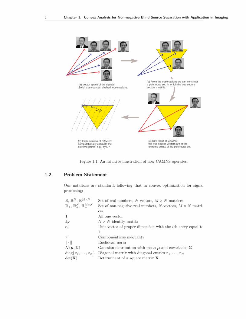
In Figure 1.1 we use diagrams to give readers some impressions on howCAMNS works.

The chapter is organized as follows. In Section 1.2, the problem statement isgiven. In Section 1.3, we review some key concepts of convex analysis, whichwould be useful for understanding of the mathematical derivations that follow.CAMNS and its resultant implications on nBSS criteria are developed in Section1.4. The systematic, analysis-based LP method for implementing CAMNS isdescribed in Section 1.5. We then introduce an alternating volume maximizationheuristics for implementing CAMNS in Section 1.6. Finally, in Section 1.7, we usesimulations to evaluate the performance of the proposed CAMNS-based nBSSmethods and some other existing nBSS methods.


(a) Vector space of the signals.Solid: true sources; dashed: observations.

(b) From the observations we can constructa polyhedral set, in which the true source vectors must lie.

(d) Implemention of CAMNS:computationally estimate the extreme points; e.g., by LP.

(c) Key result of CAMNS:the true source vectors are at the extreme points of the polyhedral set.

Figure 1.1: An intuitive illustration of how CAMNS operates.

1.2 Problem Statement

Our notations are standard, following that in convex optimization for signalprocessing:

R, RN , R

M×N Set of real numbers, N -vectors, M × N matricesR+, R

N+ , R

M×N+ Set of non-negative real numbers, N -vectors, M × N matri-

ces1 All one vectorIN N × N identity matrixei Unit vector of proper dimension with the ith entry equal to

1� Componentwise inequality‖ · ‖ Euclidean normN (μ,Σ) Gaussian distribution with mean μ and covariance Σdiag{x1, . . . , xN} Diagonal matrix with diagonal entries x1, . . . , xN

det(X) Determinant of a square matrix X


We consider the scenario of linear instantaneous mixtures of unknown sourcesignals, in which the signal model is

x[n] = As[n], n = 1, . . . , L (1.1)

where

s[n] = [ s1[n], . . . , sN [n] ]T input or source vector sequence, with N denotingthe input dimension;

x[n] = [ x1[n], . . . , xM [n] ]T output or observation vector sequence, with M

denoting the output dimension;A ∈ R

M×N mixing matrix describing the input-output rela-tion;

L sequence (or data) length, with L � max{M, N}(often true in practice).

The linear instantaneous mixture model in (1.1) can also be expressed as

xi =N∑

j=1

aijsj , i = 1, . . . , M, (1.2)

where

aij (i, j)th element of A,sj = [ sj[1], . . . , sj [L] ]T vector representing the jth source signal,xi = [ xi[1], . . . , xi[L] ]T vector representing the ith observed signal.

In blind source separation (BSS), the problem is to retrieve the sourcess1, . . . , sN from the observations x1, . . . , xM , without knowledge of A. BSSshows great potential in various applications, and here we describe two examplesin biomedical imaging.

Example 1.1: Magnetic Resonance Imaging (MRI)

Dynamic contrast-enhanced MRI (DCE-MRI) uses various molecular weightcontrast agents to assess tumor vasculature perfusion and permeability, and haspotential utility in evaluating the efficacy of angiogenesis inhibitors in cancertreatment [9]. While DCE-MRI can provide a meaningful estimation of vascula-ture permeability when a tumor is homogeneous, many malignant tumors showmarkedly heterogeneous areas of permeability, and thereby the signal at eachpixel often represents a convex mixture of more than one distinct vasculaturesource independent of spatial resolution.

The raw DCE-MRI images of breast tumor, for example, are given on the topof Figure 1.1, and its bottom plot illustrates the temporal mixing process of thesource patterns where the tumor angiogenic activities (observations) represent


=

Time

X

Time

SourcesObservations

Plasma input

Fast flowSlow flow

Region of interestextraction

DCE-MRI of breast tumor

Figure 1.2: The BSS problem in DCE-MRI applications.

the weighted summation of spatially-distributed vascular permeability associ-ated with different perfusion rates. The BSS methods can be applied to com-putationally estimate the time activity curves (mixing matrix) and underlyingcompartment vascular permeability (sources) within the tumor site.

Example 1.2: Dynamic Fluorescent Imaging (DFI)DFI exploits highly specific and biocompatible fluorescent contrast agents tointerrogate small animals for drug development and disease research [29]. Thetechnique generates a time series of images acquired after injection of an inertdye, where the dye’s differential biodistribution dynamics allow precise delin-eation and identification of major organs. However, spatial resolution and quan-titation at depth is not one of the strengths of planar optical approaches, duemainly to the malign effects of light scatter and absorption.

The DFI data acquired in a mouse study, for instance, is shown in Figure1.3, where each DFI image (observation) is delineated as a linear mixture of theanatomical maps associated with different organs. The BSS methods can be used


Time

...

Linear mixing model

Dynamic fluorescent imaging data

Kidney Lungs Brain Spine

......

Figure 1.3: The BSS problem in DFI applications.

to numerically unmix the anatomical maps (sources) and their mixing portions(mixing matrix).

1.2.1 Assumptions

Like other non-negative BSS (nBSS) techniques, the CAMNS framework to bepresented will make use of source signal non-negativity. Hence, we assume that

(A1) All sj are componentwise non-negative; i.e., for each j, sj ∈ RL+.

What makes CAMNS special compared to the other available nBSS frame-works is the use of the local dominance assumption, as follows:

(A2) Each source signal vector is local dominant, in the following sense: For eachi ∈ {1, . . . , N}, there exists an (unknown) index �i such that si[�i] > 0 andsj [�i] = 0, ∀j �= i.

In imaging, (A2) means that for each source, say source i, there exists at leastone pixel (indexed by n) such that source i has nonzero pixel while the othersources zero. It may be completely satisfied or serve as a good approximationwhen the source signals are sparse (or contain many zeros). In brain MRI, forinstance, the non-overlapping region of the spatial distribution of a fast perfusion


and a slow perfusion source images [9] can be higher than 95%. For high contrastimages such as human portraits, we found that (A2) would also be an appropriateassumption.

We make two more assumptions

(A3) The mixing matrix has unit row sum; i.e., for all i = 1, . . . , M ,

N∑j=1

aij = 1. (1.3)

(A4) M ≥ N and A is of full column rank.

Assumption (A4) is rather standard in BSS. Assumption (A3) is essential toCAMNS, but can be relaxed through a model reformulation [28]. Moreover, inMRI (e.g., in Example 1.1), (A3) is automatically satisfied due to the so-calledpartial volume effect [28]. The following example shows how we can relax (A3):

Example 1.3: Suppose that the model in (1.2) does not satisfy (A3). For simplic-ity of exposition of the idea, assume non-negative mixing; i.e., aij ≥ 0 for all (i, j)(extension to aij ∈ R is possible). Under such circumstances, the observations areall non-negative and we can assume that

xTi 1 �= 0

for all i = 1, . . . , M . Likewise, we can assume sTj 1 �= 0 for all j. The idea is to

enforce (A3) by normalizing the observation vectors:

xi � xi

xTi 1

=N∑

j=1

(aijs

Tj 1

xTi 1

)(sj

sTj 1

). (1.4)

By letting aij = aijsTj 1/xT

i 1 and sj = sj/sTj 1, we obtain a model xi =∑N

j=1 aij sj which is in the same form as the original signal model in (1.2). It iseasy to show that the new mixing matrix, denoted by A, has unit row sum [or(A3)].

It should also be noted that the model reformulation above does not damagethe rank of the mixing matrix. Specifically, if the original mixing matrix Asatisfies (A4), then the new mixing matrix A also satisfies (A4). To show this,we notice that the relationship of A and A can be expressed as

A = D−11 AD2 (1.5)

where D1 = diag(xT1 1, ..., xT

M1) and D2 = diag(sT1 1, ..., sT

N1). Since D1 and D2

are of full rank, we have rank(A) =rank(A).

Throughout this chapter, we will assume that (A1)- (A4) are satisfied unlessspecified.


1.3 Review of Some Concepts in Convex Analysis

In CAMNS we analyze the geometric structures of the signal model by utilizingsome fundamental convex analysis concepts, namely affine hull, convex hull, andtheir associated properties. As we will see in next section, such a convex analysiswill shed light into how we can separate the sources. Here we provide a reviewof the essential concepts. Readers who are interested in further details of convexanalysis are referred to the literature such as [30], [31], [32].

1.3.1 Affine Hull

Given a set of vectors {s1, . . . , sN} ⊂ RL, the affine hull is defined as

aff{s1, . . . , sN} ={

x =N∑

i=1

θisi

∣∣∣∣ θ ∈ RN ,

N∑i=1

θi = 1}

. (1.6)

Some examples of affine hulls are illustrated in Figure 1.4. We see that for N = 2,an affine hull is a line passing through s1 and s2; and for N = 3, it is a planepassing through s1, s2, and s3.

s1s1s2s2

s3

00N = 2 N = 3

aff{s1, s2}aff{s1, s2, s3}

Figure 1.4: Examples of affine hulls for N = 2 and N = 3.

An affine hull can always be represented by

aff{s1, . . . , sN} ={

x = Cα + d∣∣ α ∈ R

P}

(1.7)

for some d ∈ RL (non-unique), for some full column rank C ∈ R

L×P (also non-unique), and for some P ≥ 1. To understand this, consider a simple examplewhere {s1, . . . , sN} is linearly independent. One can verify that (1.6) can berewritten as (1.7), with

d = sN , C = [ s1 − sN , s2 − sN , . . . , sN−1 − sN ],

P = N − 1, α = [ θ1, . . . , θN−1 ]T


The number P in (1.7) is called the affine dimension, which characterizes theeffective dimension of the affine hull. The affine dimension must satisfy P ≤N − 1. Moreover,

Property 1.1. If {s1, . . . , sN} is an affinely independent set (which means that{s1 − sN , . . . , sN−1 − sN} is linearly independent), then the affine dimension ismaximal; i.e., P = N − 1.

1.3.2 Convex Hull

Given a set of vectors {s1, . . . , sN} ⊂ RL, the convex hull is defined as

conv{s1, . . . , sN} ={

x =N∑

i=1

θisi

∣∣∣∣ θ ∈ RN+ ,

N∑i=1

θi = 1}

. (1.8)

A convex hull would be a line segment for N = 2, a triangle for N = 3. This isillustrated in Figure 1.5.

s1s1

s2s2

s3

00N = 2 N = 3

conv{s1, s2} conv{s1, s2, s3}

Figure 1.5: Examples of convex hulls for N = 2 and N = 3.

An important concept related to convex hull is that of extreme points, alsoknown as vertices. From a geometric perspective, extreme points are the ‘cornerpoints’ of the convex hull. A point x ∈ conv{s1, . . . , sN} is said to be an extremepoint of conv{s1, . . . , sN} if x can never be a convex combination of s1, . . . , sN

in a non-trivial manner; i.e.,

x �=N∑

i=1

θisi (1.9)

for all θ ∈ RN+ ,∑N

i=1 θi = 1, and θ �= ei for any i. Some basic properties aboutextreme points are as follows:

Property 1.2. The set of extreme points of conv{s1, . . . , sN} must be eitherthe full set or a subset of {s1, . . . , sN}.


Property 1.3. If {s1, . . . , sN} is affinely independent, then the set of extremepoints of conv{s1, . . . , sN} is exactly {s1, . . . , sN}.

For example, in the illustrations in Figure 1.5 the extreme points are the‘corner’ points {s1, . . . , sN}.

A special, but representative case of convex hull is simplex. A convex hull iscalled a simplex if L = N − 1 and {s1, . . . , sN} is affinely independent. It followsthat

Property 1.4. The set of extreme points of a simplex conv{s1, . . . , sN} ⊂ RN−1

is {s1, . . . , sN}.

In other words, a simplex on RN−1 is a convex hull with exactly N extreme

points. A simplex for N = 2 is a line segment on R, while a simplex for N = 3is a triangle on R

2.

1.4 Non-negative Blind Source Separation Criterion via CAMNS

We now consider applying convex analysis to the nBSS problem [the model in(1.2), with assumptions (A1)- (A4)]. Such a convex analysis of mixtures of non-negative sources (CAMNS) will lead to an nBSS criterion that guarantees perfectsource separation.

1.4.1 Convex Analysis of the Problem, and the CAMNS Criterion

Recall from (1.2) that the signal model is given by

xi =N∑

j=1

aijsj , i = 1, . . . , M,

Since∑N

j=1 aij = 1 [(A3)], every xi is indeed an affine combination of{s1, . . . , sN}:

xi ∈ aff{s1, . . . , sN} (1.10)

for any i = 1, . . . , M . Hence an interesting question is the following: Can we usethe observations x1, . . . , xM to construct the source affine hull aff{s1, . . . , sN}?

To answer the question above, let us first consider the following lemma:

Lemma 1.1. The observation affine hull is identical to the source affine hull;that is,

aff{s1, . . . , sN} = aff{x1, . . . , xM}. (1.11)


An illustration is shown in Figure 1.6(a) to pictorially demonstrate the affinehull equivalence in Lemma 1.1. Since Lemma 1.1 represents an essential part toCAMNS, here we provide the proof to illustrate its idea.

s1

s2

x1

x2

x3

e1

e2

e3 aff{s1, s2} = aff{x1,x2, x3}

Figure 1.6: A geometric illustration of the affine hull equivalence in Lemma 1.1,for the special case of N = 2, M = 3, and L = 3.

Proof of Lemma 1.1. Any x ∈ aff{x1, ..., xM} can be represented by

x =M∑i=1

θixi, (1.12)

where θ ∈ RM , θT1 = 1. Substituting (1.2) into (1.12), we get

x =N∑

j=1

βjsj , (1.13)

where βj =∑M

i=1 θiaij for j = 1, ..., N , or equivalently

β = AT θ. (1.14)

Since A has unit row sum [(A3)], we have

βT1 = θT (A1) = θT1 = 1. (1.15)

This implies that βT1 = 1, and as a result it follows from (1.13) that x ∈aff{s1, ..., sN}.

On the other hand, any x ∈ aff{s1, ..., sN} can be represented by (1.13) forβT1 = 1. Since A has full column rank [(A4)], there always exist a θ such that(1.14) holds. Substituting (1.14) into (1.13) yields (1.12). Since (1.15) impliesthat θT1 = 1, we conclude that x ∈ aff{x1, ..., xM}.

Thus, by constructing the observation affine hull, the source affine hullwill be obtained. Using the linear equality representation of an affine hull,


aff{s1, . . . , sN} (or aff{x1, . . . , xM}) can be characterized as

aff{s1, . . . , sN} ={

x = Cα + d∣∣ α ∈ R

P}

(1.16)

for some (C,d) ∈ RL×P × R

L such that rank(C) = P , with P being the affinedimension. From (A2) it can be shown that (see Appendix 1.9.1)

Lemma 1.2. The set of source vectors {s1, . . . , sN} is linearly independent.

Hence, by Property 1.1 the affine dimension of aff{s1, . . . , sN} is maximal; i.e.,P = N − 1. For the special case of M = N (the number of inputs being equalto the number of outputs), it is easy to obtain (C,d) from the observationsx1, . . . , xM ; see the review in Section 1.3.

For M ≥ N , a method called affine set fitting would be required. Since (C,d)is non-unique, without loss of generality one can restrict CTC = I. The followingaffine set fitting problem is used to find (C,d)

(C,d) = arg minC,d

CT C=I

M∑i=1

eA(C,d)(xi) (1.17)

where eA(x) is the projection error of x onto A, defined as

eA(x) = minx∈A

‖x− x‖22, (1.18)

and

A(C, d) = {x = Cα + d | α ∈ RN−1} (1.19)

is an affine set parameterized by (C, d). The objective of (1.17) is to find an (N −1)-dimensional affine set that has the minimum projection error with respect tothe observations (which is zero for the noise-free case). Problem (1.17) is shownto have a closed-form solution:

Proposition 1.1. A solution to the affine set fitting problem in (1.17) is

d =1M

M∑i=1

xi (1.20)

C = [ q1(UUT ), q2(UUT ), . . . , qN−1(UUT ) ] (1.21)

where U = [ x1 − d, . . . , xM − d ] ∈ RL×M , and the notation qi(R) denotes the

eigenvector associated with the ith principal eigenvalue of the input matrix R.

The proof of the above proposition is given in Appendix 1.9.2. We should stressthat this affine set fitting provides a best affine set in terms of minimizing theprojection error. Hence, in the presence of additive noise, it has an additionaladvantage of noise mitigation for M > N .


Remember that we are dealing with non-negative sources. Hence, any sourcevector si must lie in

S � aff{s1, . . . , sN} ∩ RL+

= A(C,d) ∩ RL+

= {x | x = Cα + d, x � 0, α ∈ RN−1}. (1.22)

Note that we have knowledge of S only through (1.22), a polyhedral set repre-sentation. The following lemma plays an important role:

Lemma 1.3. The polyhedral set S is identical to the source convex hull; that is,

S = conv{s1, . . . , sN}. (1.23)

Following the illustration in Figure 1.6, in Figure 1.7 we geometrically demon-strate the equivalence of S and conv{s1, . . . , sN}. This surprising result is duemainly to the local dominance, and we include its proof here considering itsimportance.

Proof of Lemma 1.3. Assume that z ∈ aff{s1, ..., sN} ∩ RL+:

z =N∑

i=1

θisi � 0, 1T θ = 1.

From (A2), it follows that z[�i] = θisi[�i] ≥ 0, ∀i. Since si[�i] > 0, we must haveθi ≥ 0, ∀i. Therefore, z lies in conv{s1, ..., sN}. On the other hand, assume thatz ∈ conv{s1, ..., sN}, i.e.,

z =N∑

i=1

θisi, 1T θ = 1, θ � 0

implying that z ∈ aff{s1, ..., sN}. From (A1), we have si � 0 ∀i and subsequentlyz � 0. This completes the proof for (1.23).

Furthermore, we can deduce from Lemma 1.2 and Property 1.3 that

Lemma 1.4. The set of extreme points of conv{s1, . . . , sN} is {s1, . . . , sN}.

Summarizing all the results above, we establish an nBSS criterion as follows:


s1

s2e1

e2

e3

RL+ S = A(C,d)∩R

L+

= conv{s1, s2}

Figure 1.7: A geometric illustration of the convex hull equivalence in Lemma 1.3,for the special case of N = 2, M = 3, and L = 3. Note that for each si there isa coordinate along which all the other sources have zero element; specifically e3

for s1 and e1 for s2.

Criterion 1.1. Use the affine set fitting solution in Proposition 1.1 to compute(C,d). Then, find all the extreme points of the polyhedral set

S ={x ∈ R

L∣∣ x = Cα + d � 0, α ∈ R

N−1}

(1.24)

and denote the obtained set of extreme points by {s1, . . . , sN}. Output{s1, . . . , sN} as the set of estimated source vectors.

And it follows from the development above that

Theorem 1.1. The solution to Criterion 1.1 is uniquely given by the set of truesource vectors {s1, . . . , sN}, under the premises in (A1) to (A4).

The implication of Theorem 1.1 is profound: It suggests that the true sourcevectors can be perfectly identified by finding all the extreme points of S. Thisprovides new opportunities in nBSS that cannot be found in the other presentlyavailable literature to our best knowledge.

In the next section we will describe a systematic LP-based method for realizingCriterion 1.1 in practice.

1.4.2 An Alternative Form of the CAMNS Criterion

There is an alternative form to the CAMNS criterion (Criterion 1.1, specifically).The alternative form is useful for deriving simple CAMNS algorithms in some


special cases. It will also shed light into the volume maximization heuristicsconsidered in the later part of this chapter.

Consider the pre-image of the observation-constructed polyhedral set S, underthe mapping s = Cα + d:

F ={α ∈ R

N−1∣∣ Cα + d � 0

}={α ∈ R

N−1∣∣ cT

nα + dn ≥ 0, n = 1, . . . , L}

(1.25)

where cTn is the nth row of C. There is a direct correspondence between the

extreme points of S and F [26]:

Lemma 1.5. The polyhedral set F in (1.25) is equivalent to a simplex

F = conv{α1, . . . , αN} (1.26)

where each αi ∈ RN−1 satisfies

Cαi + d = si. (1.27)

The proof of Lemma 1.5 is given in Appendix 1.9.3. Since the set of extremepoints of a simplex conv{α1, . . . , αN} is {α1, . . . , αN} (Property 1.4), we havethe following alternative nBSS criterion:

Criterion 1.2 (Alternative form of Criterion 1.1). Use the affine set fittingsolution in Proposition 1.1 to compute (C,d). Then, find all the extreme pointsof the simplex

F ={α ∈ R

N−1∣∣ Cα + d � 0

}(1.28)

and denote the obtained set of extreme points by {α1, . . . , αN}. Output

si = Cαi + d, i = 1, . . . , N (1.29)

as the set of estimated source vectors.

It follows directly from Theorem 1.1 and Lemma 1.5 that

Theorem 1.2. The solution to Criterion 1.2 is uniquely given by the set of truesource vectors {s1, . . . , sN}, under the premises in (A1) to (A4).

In [26], we have used Criterion 1.2 to develop simple nBSS algorithms forthe cases of two and three sources. In the following we provide the solutionfor the two-source case and demonstrate its effectiveness using synthetic X-rayobservations:


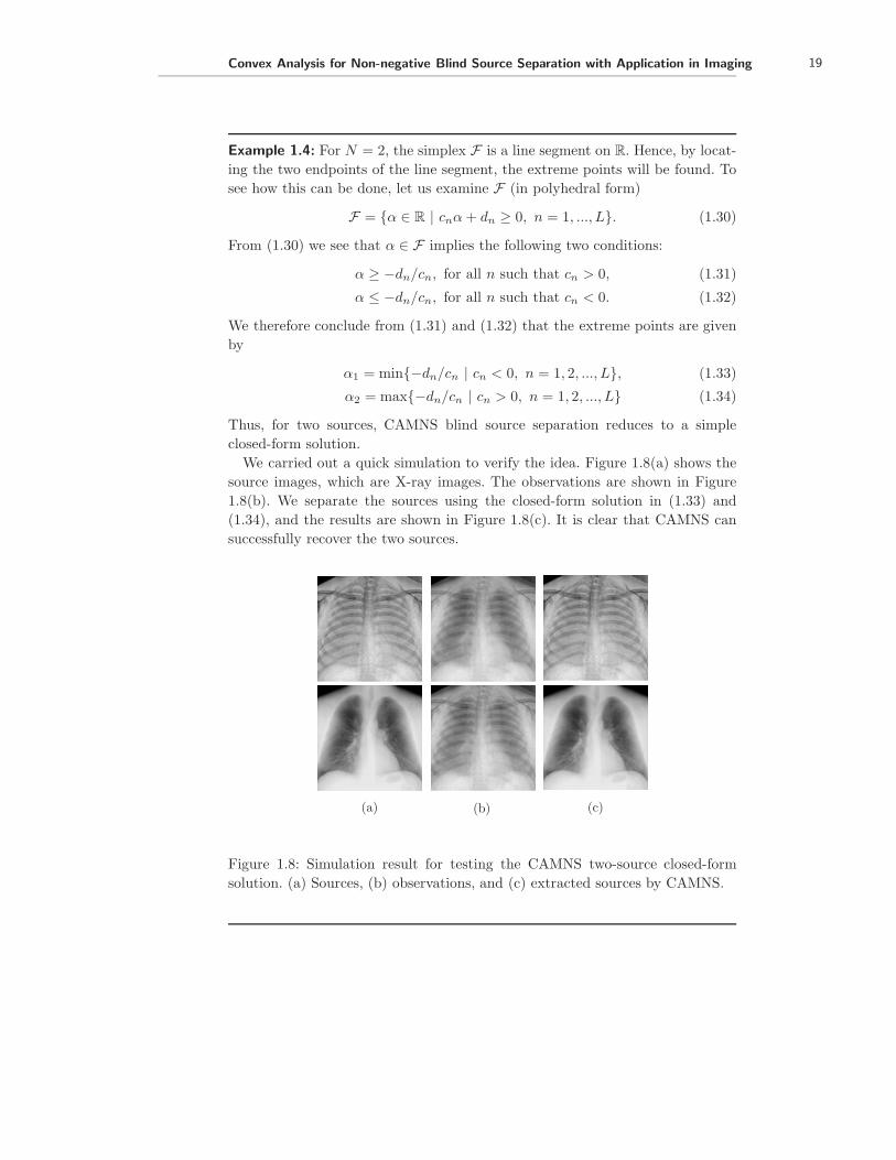
Example 1.4: For N = 2, the simplex F is a line segment on R. Hence, by locat-ing the two endpoints of the line segment, the extreme points will be found. Tosee how this can be done, let us examine F (in polyhedral form)

F = {α ∈ R | cnα + dn ≥ 0, n = 1, ..., L}. (1.30)

From (1.30) we see that α ∈ F implies the following two conditions:

α ≥ −dn/cn, for all n such that cn > 0, (1.31)

α ≤ −dn/cn, for all n such that cn < 0. (1.32)

We therefore conclude from (1.31) and (1.32) that the extreme points are givenby

α1 = min{−dn/cn | cn < 0, n = 1, 2, ..., L}, (1.33)

α2 = max{−dn/cn | cn > 0, n = 1, 2, ..., L} (1.34)

Thus, for two sources, CAMNS blind source separation reduces to a simpleclosed-form solution.

We carried out a quick simulation to verify the idea. Figure 1.8(a) shows thesource images, which are X-ray images. The observations are shown in Figure1.8(b). We separate the sources using the closed-form solution in (1.33) and(1.34), and the results are shown in Figure 1.8(c). It is clear that CAMNS cansuccessfully recover the two sources.

(a) (b) (c)

Figure 1.8: Simulation result for testing the CAMNS two-source closed-formsolution. (a) Sources, (b) observations, and (c) extracted sources by CAMNS.


1.5 Systematic Linear Programming Method for CAMNS

This section, as well as the next section are dedicated to the practical imple-mentations of CAMNS. In this section, we propose an approach that uses linearprograms (LPs) to systematically fulfil the CAMNS criterion, specifically Crite-rion 1.1. An appealing characteristic of this CAMNS-LP method is that Crite-rion 1.1 does not appear to be related to convex optimization at first look, andyet it can be exactly solved by CAMNS-LP as long as the problem assumptions(A1)-(A4) are valid.

Our problem as specified in Criterion 1.1 is to find all the extreme points of thepolyhedral set S in (1.22). In the optimization literature this problem is knownas vertex enumeration; see [33, 34, 35] and the references therein. The availableextreme-point finding methods are sophisticated, requiring no assumption onthe extreme points. However, the complexity of those methods would increaseexponentially with the number of inequalities L (note that L is also the datalength in our problem, which is often large in practice). The notable difference ofthe development here is that we exploit the characteristic that the extreme pointss1, ..., sN are linearly independent (Lemma 1.2). By doing so we will establishan extreme-point finding method (for CAMNS) whose complexity is polynomialin L.

Our approach is to identify one extreme point at one time. Consider the fol-lowing linear minimization problem:

p� = mins

rT s

subject to (s.t.) s ∈ S(1.35)

for some arbitrarily chosen direction r ∈ RL, where p� denotes the optimal objec-

tive value of (1.35). By the polyhedral representation of S in (1.22), problem(1.35) can be equivalently represented by an LP

p� = minα

rT (Cα + d)

s.t. Cα + d � 0(1.36)

which can be solved by readily available algorithms such as the polynomial-time interior-point methods [36, 37]. Problem (1.36) is the problem we solve inpractice, but (1.35) leads to important implications to extreme-point search.

A fundamental result in LP theory is that rT s, the objective function of (1.35),attains the minimum at a point of the boundary of S. To provide more insights,some geometric illustrations are given in Figure 1.9. We can see that the solutionof (1.35) may be uniquely given by one of the extreme points si [Figure 1.9(a)],or it may be any point on a face [Figure 1.9(b)]. The latter case poses a trouble toour task of identifying si, but it is arguably not a usual situation. For instance,in the illustration in Figure 1.9(b), r must be normal to s2 − s3 which may beunlikely to happen for a randomly picked r. With this intuition in mind, we canprove the following lemma:


Lemma 1.6. Suppose that r is randomly generated following a distributionN (0, IL). Then, with probability 1, the solution of (1.35) is uniquely given bysi for some i ∈ {1, ..., N}.

0

r

s1

s2

s3

(a)

S

optimal point

0

r

s1

s2

s3

(b)

S

set of optimal points

Figure 1.9: Geometric interpretation of an LP.

The proof of Lemma 1.6 is given in Appendix 1.9.4. The idea behind the proofis that undesired cases, such as that in Figure 1.9(b) happen with probabilityzero.

We may find another extreme point by solving the maximization counterpartof (1.35)

q� = maxα

rT (Cα + d)

s.t. Cα + d � 0.(1.37)

Using the same derivations as above, we can show the following: Under thepremise of Lemma 1.6, the solution of (1.37) is, with probability 1, uniquelygiven by an extreme point si different from that in (1.35).

Suppose that we have identified l extreme points, say, without loss of gener-ality, {s1, ..., sl}. Our interest is in refining the above LP extreme-point findingprocedure such that the search space is restricted to {sl+1, ..., sN}. To do so,consider a thin QR decomposition [38] of [s1, ..., sl]

[s1, ..., sl] = Q1R1, (1.38)

where Q1 ∈ RL×l is semi-unitary and R1 ∈ R

l×l is upper triangular. Let

B = IL − Q1QT1 . (1.39)

We assume that r takes the form

r = Bw (1.40)

for some w ∈ RL, and consider solving (1.36) and (1.37) with such an r. Since

r is orthogonal to the old extreme points s1, ..., sl, the intuitive expectation is


that (1.36) and (1.37) should both lead to new extreme points. Interestingly, wefound theoretically that such an expectation is not true, but close. It can beshown that (see Appendix 1.9.5)

Lemma 1.7. Suppose that r = Bw, where B ∈ RL×L is given by (1.39) and w

is randomly generated following a distribution N (0, IL). Then, with probability1, at least one of the optimal solutions of (1.36) and (1.37) is a new extremepoint; i.e., si for some i ∈ {l + 1, ..., N}. The certificate of finding new extremepoints is indicated by |p�| �= 0 for the case of (1.36), and |q�| �= 0 for (1.37).

By repeating the above described procedures, we can identify all the extremepoints s1, ..., sN . The resultant CAMNS-LP method is summarized in Algorithm1.1.

Algorithm 1.1. CAMNS-LP

Given an affine set characterization 2-tuple (C,d).Step 1. Set l = 0, and B = IL.

Step 2. Randomly generate a vector w ∼ N (0, IL), and set r := Bw.Step 3. Solve the LPs

p� = minα:Cα+d�0

rT (Cα + d)

q� = maxα:Cα+d�0

rT (Cα + d)

and obtain their optimal solutions, denoted by α�1 and α�

2, respectively.Step 4. If l = 0

S = [ Cα�1 + d, Cα�

2 + d ]else

If |p�| �= 0 then S := [ S Cα�1 + d ].

If |q�| �= 0 then S := [ S Cα�2 + d ].

Step 5. Update l to be the number of columns of S.Step 6. Apply QR decomposition

S = Q1R1,

where Q1 ∈ RL×l and R1 ∈ R

l×l. Update B := IL − Q1QT1 .

Step 7. Repeat Step 2 to Step 6 until l = N .

The CAMNS-LP method in Algorithm 1.1 is not only systematically straight-forward to apply, it is also efficient due to the maturity of convex optimiza-tion algorithms. Using a primal-dual interior-point method, each LP problem [orthe problem in (1.35) or (1.37)] can be solved with a worst-case complexity ofO(L0.5(L(N − 1) + (N − 1)3)) O(L1.5(N − 1)) for L � N [37]. Since the algo-


rithm solves 2(N − 1) LP problems in the worst case, we infer that its worst-casecomplexity is O(L1.5(N − 1)2).

Based on Theorem 1.1, Lemma 1.6, Lemma 1.7, and the complexity discussionabove, we conclude that

Proposition 1.2. Algorithm 1.1 finds all the true source vectors s1, ..., sN withprobability 1, under the premises of (A1)-(A4). It does so with a worst-case com-plexity of O(L1.5(N − 1)2).

We have provided a practical implementation of CAMNS-LP at http:

//www.ee.cuhk.edu.hk/∼wkma/CAMNS/CAMNS.htm. The source codes were writ-ten in MATLAB, and are based on the reliable convex optimization softwareSeDuMi [36]. Readers are encouraged to test the codes and give us some feed-back.

1.6 Alternating Volume Maximization Heuristics for CAMNS

The CAMNS-LP method developed in the last section elegantly takes advantageof the model assumptions to sequentially track down the extreme points or thetrue source vectors. In particular, the local dominant assumption (A2) plays akey role. Our simulation experience is that CAMNS-LP can provide good sepa-ration performance on average, even when the local dominance assumption is notperfectly satisfied. In this section we consider an alternative that is also inspiredby the CAMNS criterion, and that is intuitively expected to offer better robust-ness against model mismatch with local dominance. As we will further explainsoon, the idea is to perform simplex volume maximization. Unfortunately suchan attempt will lead us to a nonconvex optimization problem. We will proposean alternating, LP-based optimization heuristics to the simplex volume maxi-mization problem. Although the alternating heuristics is suboptimal, simulationresults will indicate that the alternating heuristics can provide a better sepa-ration than CAMNS-LP, by a factor of about several dBs in sum-square-errorperformance (for data where local dominance is not perfectly satisfied).

Recall the CAMNS criterion in Criterion 1.2: Find the extreme points of thepolyhedral set

F ={α ∈ R

N−1∣∣ Cα + d � 0

}which, under the model assumptions in (A1)-(A4), is a simplex in form of

F = conv{α1, . . . , αN}.For a simplex we can define its volume: A simplex, say denoted byconv{β1, . . . , βN} ⊂ R

N−1, has its volume given by [39]

V (β1, . . . , βN ) =|det (Δ(β1, . . . , βN ))|

(N − 1)!, (1.41)


where

Δ(β1, . . . , βN ) =[

β1 · · · βN

1 · · · 1

]∈ R

N×N . (1.42)

Suppose that {β1, . . . , βN} ⊂ F . As illustrated in the picture in Fig-ure 1.10, the volume of conv{β1, . . . , βN} should be no greater than thatof F = conv{α1, . . . , αN}. Hence, by finding {β1, . . . , βN} ⊂ F such that therespective simplex volume is maximized, we would expect that {β1, . . . , βN}is exactly {α1, . . . , αN}, the ground truth we are seeking. This leads to thefollowing variation of the CAMNS criterion:

F

β1 β2

β3

α1

α2

α3

conv{β1,β2,β3}

Figure 1.10: A geometric illustration for {β1, . . . , βN} ⊂ F for N = 3.

Criterion 1.3 (Volume maximization alternative to Criterion 1.2). Use theaffine set fitting solution in Proposition 1.1 to compute (C,d). Then, solve thevolume maximization problem

{α1, . . . , αN} = arg maxβ1,...,βN

V (β1, . . . , βN )

s.t. {β1, . . . , βN} ⊂ F ,(1.43)

Output

si = Cαi + d, i = 1, . . . , N (1.44)

as the set of estimated source vectors.

Like Criteria 1.1 and 1.2, Criterion 1.3 can be shown to provide the sameperfect separation result

Theorem 1.3. The globally optimal solution of (1.43) is uniquely given byα1, . . . , αN , under the premises of (A1)-(A4).


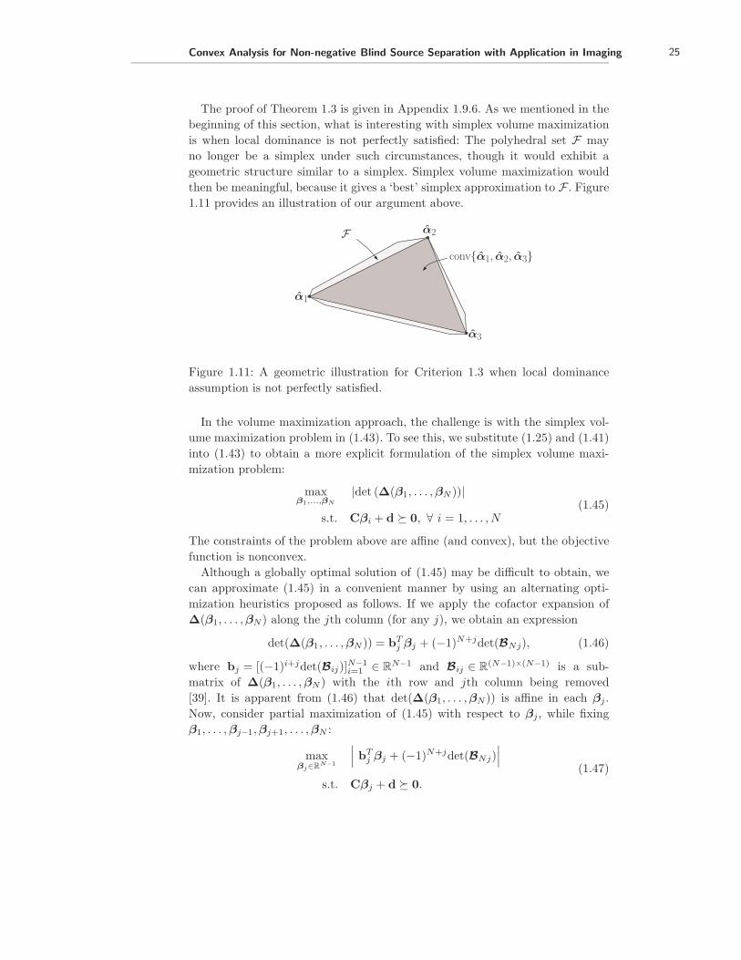
The proof of Theorem 1.3 is given in Appendix 1.9.6. As we mentioned in thebeginning of this section, what is interesting with simplex volume maximizationis when local dominance is not perfectly satisfied: The polyhedral set F mayno longer be a simplex under such circumstances, though it would exhibit ageometric structure similar to a simplex. Simplex volume maximization wouldthen be meaningful, because it gives a ‘best’ simplex approximation to F . Figure1.11 provides an illustration of our argument above.

F

α1

α2

α3

conv{α1, α2, α3}

Figure 1.11: A geometric illustration for Criterion 1.3 when local dominanceassumption is not perfectly satisfied.

In the volume maximization approach, the challenge is with the simplex vol-ume maximization problem in (1.43). To see this, we substitute (1.25) and (1.41)into (1.43) to obtain a more explicit formulation of the simplex volume maxi-mization problem:

maxβ1,...,βN

|det (Δ(β1, . . . , βN ))|

s.t. Cβi + d � 0, ∀ i = 1, . . . , N(1.45)

The constraints of the problem above are affine (and convex), but the objectivefunction is nonconvex.

Although a globally optimal solution of (1.45) may be difficult to obtain, wecan approximate (1.45) in a convenient manner by using an alternating opti-mization heuristics proposed as follows. If we apply the cofactor expansion ofΔ(β1, . . . , βN) along the jth column (for any j), we obtain an expression

det(Δ(β1, . . . , βN )) = bTj βj + (−1)N+jdet(BNj), (1.46)

where bj = [(−1)i+jdet(Bij)]N−1i=1 ∈ R

N−1 and Bij ∈ R(N−1)×(N−1) is a sub-

matrix of Δ(β1, . . . , βN) with the ith row and jth column being removed[39]. It is apparent from (1.46) that det(Δ(β1, . . . , βN)) is affine in each βj.Now, consider partial maximization of (1.45) with respect to βj, while fixingβ1, . . . , βj−1, βj+1, . . . , βN :

maxβj∈R

N−1

∣∣∣ bTj βj + (−1)N+jdet(BNj)

∣∣∣s.t. Cβj + d � 0.

(1.47)


The objective function in (1.47) is still nonconvex, but (1.47) can be solved in aglobally optimal manner by breaking it into two LPs:

p� = maxβj∈R

N−1bT

j βj + (−1)N+jdet(BNj)

s.t. Cβj + d � 0.(1.48)

q� = minβj∈R

N−1bT

j βj + (−1)N+jdet(BNj)

s.t. Cβj + d � 0.(1.49)

The optimal solution of (1.47), denoted by αj , is the optimal solution of (1.48) if|p�| > |q�|, and the optimal solution of (1.49) if |q�| > |p�|. This partial maximiza-tion is conducted alternately (i.e., j := (j modulo N) + 1) until some stoppingrule is satisfied.

The CAMNS alternating volume maximization heuristics, or simply CAMNS-AVM, is summarized in Algorithm 1.2.


Algorithm 1.2. CAMNS-AVM

Given a convergence tolerance ε > 0, an affine set characterization 2-tuple(C,d), and the observations x1, . . . , xM .

Step 1. Initialize β1, . . . , βN ∈ F . (our suggested choice: Randomlychoose N vectors out of the M observation-constructed vectors{ (CT C)−1CT (xi − d), i = 1, . . . , M }). Set

Δ(β1, . . . , βN ) =[

β1 · · · βN

1 · · · 1

],

� := | det(Δ(β1, . . . , βN ))|, and j := 1.Step 2. Update Bij by a submatrix of Δ(β1, . . . , βN ) with the ith row and jth

column removed, and bj := [(−1)i+jdet(Bij)]N−1i=1 .

Step 3. Solve the LPs

p� = maxβj :Cβj+d�0

bTj βj + (−1)N+jdet(BNj)

q� = minβj :Cβj+d�0

bTj βj + (−1)N+jdet(BNj)

and obtain their optimal solutions, denoted by βj and βj, respectively.

Step 4. If |p�| > |q�|, then update βj := βj . Otherwise, update βj := βj.

Step 5. If (j modulo N) �= 0, then j := j + 1, and go to Step 2,else

If |max{|p�|, |q�|} − �|/� < ε, then αi = βi for i = 1, . . . , N .Otherwise, set � := max{|p�|, |q�|}, j := 1, and go to Step 2.

Step 6. Compute the source estimates s1, . . . , sN through sj = Cαj + d.

Like alternating optimization in many other applications, the number of iter-ations required for CAMNS-AVM to terminate may be difficult to analyze. Inthe simulations considered in the next section, we found that for an accuracyof ε = 10−13, CAMNS-AVM takes about 2 to 4 iterations to terminate, which issurprisingly quite small. Following the same complexity evaluation as in CAMNS-LP, CAMNS-AVM has a complexity of O(N2L1.5) per iteration. This means thatCAMNS-AVM is only about 2 to 4 times more expensive than CAMNS-LP (byempirical experience).

1.7 Numerical Results

To demonstrate the efficacy of the CAMNS-LP and CAMNS-AVM methods,four simulation results are presented here. Section 1.7.1 is a cell image exam-ple where our task is to distinguish different types of cells. Section 1.7.2 focuses


on a challenging scenario reminiscent of ghosting effects in photography. Sec-tion 1.7.3 considers a problem in which the sources are faces of five differentpersons. Section 1.7.4 uses Monte Carlo simulation to evaluate the performanceof CAMNS-based algorithms under noisy condition. For performance compari-son, we also test three existing nBSS algorithms, namely non-negative matrixfactorization (NMF) [16], non-negative independent component analysis (nICA)[12], and Ergodan’s algorithm (a BSS method that exploits magnitude boundsof the sources) [6].

The performance measure used in this book chapter is described as follows. LetS = [s1, . . . , sN ] be the true multi-source signal matrix, and S = [s1, . . . , sN ] bethe multi-source output of a BSS algorithm. It is well known that a BSS algorithmis inherently subject to permutation and scaling ambiguities. We propose a sumsquare error (SSE) measure for S and S [40, 41], given as follows:

e(S, S) = minπ∈ΠN

N∑i=1

∥∥∥∥si − ‖si‖‖sπi

‖ sπi

∥∥∥∥2

(1.50)

where π = (π1, . . . , πN ), and ΠN = {π ∈ RN | πi ∈ {1, 2, . . . , N}, πi �= πj for i �=

j} is the set of all permutations of {1, 2, ..., N}. The optimization of (1.50) is toadjust the permutation π such that the best match between true and estimatedsignals is yielded, while the factor ‖si‖/‖sπi

‖ is to fix the scaling ambiguity.Problem (1.50) is the optimal assignment problem which can be efficiently solvedby Hungarian algorithm 1 [42].

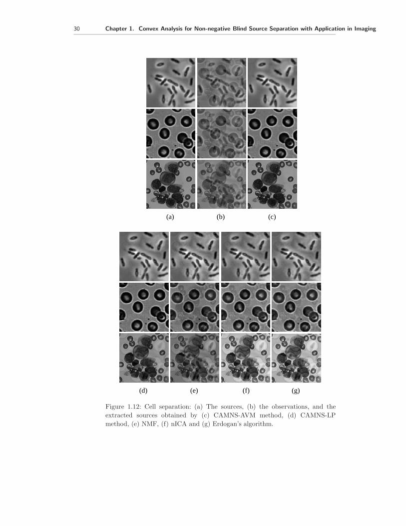
1.7.1 Example of 3-Source Case: Cell Separation

In this example three 125 × 125 cell images, displayed in Figure 1.12(a), weretaken as the source images. Each image is represented by a source vector si ∈ R

L,by scanning the image vertically from top left to bottom right (thereby L =1252 = 15625). For the three source images, we found that the local dominanceassumption is not perfectly satisfied. To shed some light into this, we propose ameasure called the local dominance proximity factor (LDPF) of the ith source,defined as follows:

κi = maxn=1,...,L

si[n]∑j �=i sj [n]

. (1.51)

When κi = ∞, we have the ith source satisfying the local dominance assumptionperfectly. The values of κi’s in this example are shown in Table 1.1, where wesee that the LDPFs of the three sources are strong but not infinite.

1 A Matlab implementation is available at http://si.utia.cas.cz/Tichavsky.html.


Table 1.1. Local dominance proximity factors in the three scenarios.

κi

source 1 source 2 source 3 source 4 source 5

Cell separation 48.667 3.821 15.200 - -

Ghosting reduction 2.133 2.385 2.384 2.080 -

Human face separation 10.450 9.107 5.000 3.467 2.450

Table 1.2. The SSEs of the various nBSS methods in the three scenarios.

SSE e(S, S) (in dB)CAMNS-AVM CAMNS-LP NMF nICA Erdogan’s algorithm

Cell separation 3.710 12.323 23.426 19.691 19.002

Ghosting reduction 11.909 20.754 38.620 41.896 39.126

Human face separation 0.816 17.188 39.828 43.581 45.438

The three observation vectors are synthetically generated using a mixingmatrix

A =

⎡⎣ 0.20 0.62 0.18

0.35 0.37 0.280.40 0.40 0.20

⎤⎦ . (1.52)

The mixed images are shown in Figure 1.12(b). The separated images of thevarious nBSS methods are illustrated in Figure 1.12(c)-(g). By visual inspec-tion, the CAMNS-based methods provide good separation, despite the fact thatthe local dominance assumption is not perfectly satisfied. This result indicatesthat the CAMNS-based methods have some robustness against violation of localdominance. The SSE performance of the various methods is given in Table 1.2.We observe that the CAMNS-AVM method yields the best performance amongall the methods under test, and then followed by CAMNS-LP. This suggeststhat CAMNS-AVM is more robust than CAMNS-LP, when local dominance isnot exactly satisfied. This result will be further confirmed in the Monte Carlosimulation in Section 1.7.4.

1.7.2 Example of 4-Source Case: Ghosting Effect

We take a 285 × 285 Lena image from [2] as one source and then shift it diagonallyto create three more sources; see Figure 1.13(a). Apparently, these sources arestrongly correlated. Even worse, their LDPFs, shown in Table 1.1 are not toosatisfactory compared to the previous example. The mixing matrix is

A =

⎡⎢⎢⎣

0.02 0.37 0.31 0.300.31 0.21 0.26 0.220.05 0.38 0.28 0.290.33 0.23 0.21 0.23

⎤⎥⎥⎦ . (1.53)


(a) (b) (c)

(d) (e) (f) (g)

Figure 1.12: Cell separation: (a) The sources, (b) the observations, and theextracted sources obtained by (c) CAMNS-AVM method, (d) CAMNS-LPmethod, (e) NMF, (f) nICA and (g) Erdogan’s algorithm.


Figure 1.13(b) displays the observations, where the mixing effect is reminis-cent of the ghosting effect in analog televisions. The image separation resultsare illustrated in Figure 1.13(c)-(g). Clearly, only the CAMNS-based methodsprovide sufficiently good mitigation of the “ghosts”. This result once again sug-gests that the CAMNS-based methods is not too sensitive to the effect of localdominance violation. The numerical results shown in Table 1.2 reflect that theSSE of CAMNS-AVM is about 9 dB smaller than that of CAMNS-LP, whichcan be validated by visual inspection on Figure 1.13(d) where there are slightresiduals on the 4th separated image. We argue that the residuals are harder tonotice for the CAMNS-AVM method.

1.7.3 Example of 5-Source Case: Human Face Separation

Five 240 × 320 photos taken from the second author and his friends are used asthe source images in this example; see Figure 1.14(a). Since each human face wascaptured almost at the same position, the source images have some correlations.Once again, the local dominance assumption is not perfectly satisfied as shownin Table 1.1. The five mixed images, displayed in Figure 1.14(b) are generatedthrough a mixing matrix given by

A =

⎡⎢⎢⎢⎢⎣

0.01 0.05 0.35 0.21 0.380.04 0.14 0.26 0.20 0.360.23 0.26 0.19 0.28 0.040.12 0.23 0.19 0.22 0.240.29 0.32 0.02 0.12 0.25

⎤⎥⎥⎥⎥⎦ . (1.54)

Figures 1.14(c)-(g) show the separated images of the various nBSS methods.Apparently, one can see that the CAMNS-based methods have more accurateseparation than the other methods, except some slight residual image appear-ing in the 2nd CAMNS-LP separated image, by careful visual inspection. Thenumerical results shown in Table 1.2 indicate that the CAMNS-based methodsperform better than the other methods. Moreover, comparing CAMNS-AVM andCAMNS-LP, there is a large performance gap of about 16 dB.

1.7.4 Monte Carlo Simulation: Noisy Environment

We use Monte Carlo simulation to test the performance of the various methodswhen noise is present. The three cell images in Figure 1.12(a) were used to gener-ate six noisy observations. The noise is independent and identically distributed(i.i.d.), following a Gaussian distribution with zero mean and variance σ2. Tomaintain non-negativity of the observations in the simulation, we force the nega-tive noisy observations to zero. We performed 100 independent runs. At each runthe mixing matrix was i.i.d. uniformly generated on [0,1] and then each row wasnormalized to 1 to maintain (A3). The average SSE for different SNRs (defined


(a)

(b)

(c)

(d)

(e)

(f)

(g)

Figure 1.13: Ghosting reduction: (a) The sources, (b) the observations, andthe extracted sources obtained by (c) CAMNS-AVM method, (d) CAMNS-LPmethod, (e) NMF, (f) nICA and (g) Erdogan’s algorithm.


(a) (b) (c) (d)

Figure 1.14: Human face separation: (a) The sources, (b) the observations, andthe extracted sources obtained by (c) CAMNS-AVM method and (d) CAMNS-LP method.

here as SNR=∑N

i=1 ‖si‖2/LNσ2) are shown in Figure 1.15. One can see thatthe CAMNS-based methods perform better than the other methods.

We examine the performance of the various methods for different numberof noisy observations with fixed SNR= 25 (dB). The average SSE for the var-ious methods are shown in Figure 1.16. One can see that the performance ofCAMNS-based methods become better when more observations are given. Thisphenomenon clearly validates the noise mitigation merit of the affine set fittingprocedure (Proposition 1.1) in CAMNS.


(e) (f) (g)

Figure 1.14: Human face separation (continued): The extracted sources obtainedby (e) NMF, (f) nICA and (g) Erdogan’s algorithm.

1.8 Summary and Discussion

In this book chapter, we have shown how convex analysis provides a new avenueto approaching non-negative blind source separation. Using convex geometryconcepts such as affine hull and convex hull, an analysis was carried out toshow that under some appropriate assumptions nBSS can be boiled down toa problem of finding extreme points of a polyhedral set. We have also shownhow this extreme point finding problem can be solved by convex optimization,specifically by using LPs to systematically find all the extreme points.

The key success of this new nBSS framework is based on a deterministic signalassumption called local dominance. Local dominance is a good model assump-tion for sparse or high-contrast images, but it may not be perfectly satisfied


20 25 30 35

18

20

22

24

26

28

30

32

SNR (dB)

Ave

rage

SS

E (

dB)

Erdogan’s algorithmNMFnICACAMNS−LPCAMNS−AVM

Figure 1.15: Performance evaluation of the CAMNS-based methods, NMF, nICAand Erdogan’s method for the cell images experiment for different SNRs.

sometimes. We have developed an alternative to the systematic LP method thatis expected to yield better robustness against violation of local dominance. Theidea is to solve a volume maximization problem. Despite the fact that the pro-posed algorithm uses heuristics to handle volume maximization (which is non-convex), simulation results match with our intuitive expectation that volumemaximization (done by a heuristics) can exhibit better resistance against themodel mismatch.

We have carried out a number of simulations using different sets of imagedata, and have demonstrated that the proposed convex analysis based nBSSmethods are promising, both by visual inspection and by the sum-square-errorseparation performance measure. Other methods such as nICA and NMF werealso compared to demonstrate the effectiveness of the proposed methods.


6 8 10 12 14 16

18

20

22

24

26

28

30

32

Number of observations

Ave

rage

SS

E (

dB)

Erdogan’s algorithmNMFnICACAMNS−LPCAMNS−AVM

Figure 1.16: Performance evaluation of the CAMNS-based methods, NMF, nICAand Erdogan’s method for the cell images experiment for different number ofnoisy observations.

1.9 Appendix

1.9.1 Proof of Lemma 1.2

We prove the linear independence of s1, . . . , sN by showing that∑N

j=1 θjsj = 0only has the trivial solution θ1 = θ2 = . . . = θL = 0.

Suppose that∑N

j=1 θjsj = 0 is true. Under (A2), for each source i we have the�ith entry (the local dominant point) of

∑Nj=1 θjsj given by

0 =N∑

j=1

θjsj [�i] = θisi[�i]. (1.55)

Since si[�i] > 0, we must have θi = 0 and this has to be satisfied for all i. As aresult, Lemma 1.2 is obtained.

1.9.2 Proof of Proposition 1.1

As a basic result in least squares, each projection error in (1.17)

eA(C,d)(xi) = minα∈R

N−1‖Cα + d− xi‖2

2 (1.56)

has a closed form

eA(C,d)(xi) = (xi − d)T P⊥C

(xi − d) (1.57)


where P⊥C

is the orthogonal complement projection of C. Using (1.57), the affineset fitting problem [in (1.17)] can be rewritten as

minCT C=I

{mind

M∑i=1

(xi − d)TP⊥C

(xi − d)

}. (1.58)

The inner minimization problem in (1.58) is an unconstrained convex quadraticprogram, and it can be easily verified that d = 1

M

∑Mi=1 xi is an optimal solution

to the inner minimization problem. By substituting this optimal d into (1.58)and by letting U = [x1 − d, ..., xM − d], problem (1.58) can be reduced to

minCT C=IN−1

Trace{UTP⊥CU}. (1.59)

When CT C = IN−1, the projection matrix P⊥C

can be simplified to IL − CCT .Subsequently (1.59) can be further reduced to

maxCT C=IN−1

Trace{UT CCTU}. (1.60)

An optimal solution of (1.60) is known to be the N − 1 principal eigenvectormatrix of UUT [38] as given by (1.21).


Equation (1.25) can also be expressed as

F ={

α ∈ RN−1 | Cα + d ∈ conv{s1, ..., sN} } .

Thus, every α ∈ F satisfies

Cα + d =N∑

i=1

θisi (1.61)

for some θ � 0, θT1 = 1. Since C has full column rank, (1.61) can be re-expressed as

α =N∑

i=1

θiαi, (1.62)

where αi = (CT C)−1CT (si − d) (or Cαi + d = si). Equation (1.62) impliesthat F = conv{α1, ..., αN}.

We now show that F = conv{α1, ..., αN} is a simplex by contradiction. Sup-pose that {α1, ..., αN} are not affinely independent. This means that for someγ1, . . . , γN−1,

∑N−1i=1 γi = 1, αN =

∑N−1i=1 γiαi can be satisfied. One then has

sN = CαN + d =∑N−1

i=1 γisi, which is a contradiction to the property that{s1, ..., sN} is linearly independent.



Any point in S = conv{s1, ..., sN} can be equivalently represented by s =∑Ni=1 θisi, where θ � 0 and θT1 = 1. Applying this result to (1.35), problem

(1.35) can be reformulated as

minθ∈RN

∑Ni=1 θiρi

s.t. θT1 = 1, θ � 0,(1.63)

where ρi = rT si. We assume without loss of generality that ρ1 < ρ2 ≤ · · · ≤ ρN .If ρ1 < ρ2 < · · · < ρN , then it is easy to verify that the optimal solution to (1.63)is uniquely given by θ� = e1. In its counterpart in (1.35), this translates intos� = s1. But when ρ1 = ρ2 = · · · = ρP and ρP < ρP+1 ≤ · · · ≤ ρN for some P ,the solution of (1.63) is not unique. In essence, the latter case can be shown tohave a solution set

Θ� = {θ | θT1 = 1, θ � 0, θP+1 = ... = θN = 0}. (1.64)

We now prove that the non-unique solution case happens with probabilityzero. Suppose that ρi = ρj for some i �= j, which means that

(si − sj)T r = 0. (1.65)

Let v = (si − sj)T r. Apparently, v follows a distribution N (0, ‖si − sj‖2). Sincesi �= sj , the probability Pr[ρi = ρj ] = Pr[v = 0] is of measure zero. This in turnimplies that ρ1 < ρ2 < · · · < ρN holds with probability 1.


The approach to proving Lemma 1.7 is similar to that in Lemma 1.6. Let

ρi = rT si = (Bw)T si (1.66)

for which we have ρi = 0 for i = 1, ..., l. It can be shown that

ρl+1 < ρl+2 < · · · < ρN (1.67)

holds with probability 1, as long as {s1, . . . , sN} is linearly independent. Prob-lems (1.35) and (1.37) are respectively equivalent to

p� = minθ∈RN

N∑i=l+1

θiρi

s.t. θ � 0, θT1 = 1,

(1.68)

q� = maxθ∈RN

N∑i=l+1

θiρi

s.t. θ � 0, θT1 = 1.

(1.69)


Assuming (1.67), we have three distinct cases to consider: (C1) ρl+1 < 0, ρN < 0,(C2) ρl+1 < 0, ρN > 0, and (C3) ρl+1 > 0, ρN > 0.

For (C2), we can see the following: Problem (1.68) has a unique optimal solu-tion θ� = el+1 [and s� = sl+1 in its counterpart in (1.35)], attaining an optimalvalue p� = ρl+1 < 0. Problem (1.69) has a unique optimal solution θ� = eN [ands� = sN in its counterpart in (1.37)], attaining an optimal value q� = ρN > 0.In other words, both (1.68) and (1.69) lead to finding new extreme points. For(C1), problem (1.69) is shown to have a solution set

Θ� = {θ | θT1 = 1, θ � 0, θl+1 = · · · = θN = 0}, (1.70)

which contains convex combinations of the old extreme points, and the optimalvalue is q� = 0. Nevertheless, it is still true that (1.68) finds a new extreme pointwith p� < 0. A similar situation happens with (C3), where (1.68) does not finda new extreme point with p� = 0, but (1.69) finds a new extreme point withq� > 0.

1.9.6 Proof of Theorem 1.3

In problem (1.43), the constraints βi ∈ F = conv{α1, . . . , αN} imply that

βi =N∑

j=1

θijαj (1.71)

where∑N

j=1 θij = 1 and θij ≥ 0 for i = 1, . . . , N . Hence we can write

Δ(β1, . . . , βN) = Δ(α1, . . . , αN )ΘT , (1.72)

where Θ = [θij ] ∈ RN×N+ and Θ1 = 1. For such a structured Θ it was shown

that (Lemma 1 in [43])

|det (Θ)| ≤ 1 (1.73)

and that |det (Θ)| = 1 if and only if Θ is a permutation matrix. It follows from(1.41), (1.72) and (1.73) that

V (β1, . . . , βN) =|det(Δ(α1, . . . , αN )ΘT )|/(N − 1)!

= |det(Δ(α1, . . . , αN ))||det(Θ)|/(N − 1)!

≤ V (α1, . . . , αN ) (1.74)

and that the equality holds if and only if Θ is a permutation matrix, whichimplies {β1, . . . , βN} = {α1, . . . , αN}. Hence we conclude that V (β1, . . . , βN) ismaximized if and only if {β1, . . . , βN} = {α1, . . . , αN}.


Acknowledgments

This work was supported in part by the National Science Council (R.O.C.) underGrants NSC 96-2628-E-007-003-MY3, by the U.S. National Institutes of Healthunder Grants EB000830 and CA109872, and by a grant from the Research GrantCouncil of Hong Kong (General Research Fund, Project 2150599).

References

[1] A. Hyvarinen, J. Karhunen, and E. Oja, Independent Component Analysis.New York: John Wiley, 2001.

[2] A. Cichocki and S. Amari, Adaptive Blind Signal and Image Processing.John Wiley and Sons, Inc., 2002.

[3] L. Parra and C. Spence, “Convolutive blind separation of non-stationarysources,” IEEE Trans. Speech Audio Process., vol. 8, no. 3, pp. 320–327,2000.

[4] D.-T. Pham and J.-F. Cardoso, “Blind separation of instantaneous mixturesof nonstationary sources,” IEEE Trans. Signal Process., vol. 49, no. 9, pp.1837–1848, 2001.

[5] A. Prieto, C. G. Puntonet, and B. Prieto, “A neural learning algorithm forblind separation of sources based on geometric properties,” Signal Process-ing, vol. 64, pp. 315–331, 1998.

[6] A. T. Erdogan, “A simple geometric blind source separation method forbound magnitude sources,” IEEE Trans. Signal Process., vol. 54, no. 2, pp.438–449, 2006.

[7] F. Vrins, J. A. Lee, and M. Verleysen, “A minimum-range approach to blindextraction of bounded sources,” IEEE Trans. Neural Netw., vol. 18, no. 3,pp. 809–822, 2006.

[8] J. M. P. Nascimento and J. M. B. Dias, “Does independent componentanalysis play a role in unmixing hyperspectral data?” IEEE Trans. Geosci.Remote Sensing, vol. 43, no. 1, pp. 175–187, Jan. 2005.

[9] Y. Wang, J. Xuan, R. Srikanchana, and P. L. Choyke, “Modeling and recon-struction of mixed functional and molecular patterns,” Intl. J. Biomed.Imaging, p. ID29707, 2006.

[10] N. Keshava and J. Mustard, “Spectral unmixing,” IEEE Signal Process.Mag., vol. 19, no. 1, pp. 44–57, Jan. 2002.

[11] E. R. Malinowski, Factor Analysis in Chemistry. New York: John Wiley,2002.

[12] M. D. Plumbley, “Algorithms for non-negative independent componentanalysis,” IEEE Trans. Neural Netw., vol. 14, no. 3, pp. 534–543, 2003.

[13] S. A. Astakhov, H. Stogbauer, A. Kraskov, and P. Grassberger, “MonteCarlo algorithm for least dependent non-negative mixture decomposition,”Analytical Chemistry, vol. 78, no. 5, pp. 1620–1627, 2006.

41

42 References

[14] S. Moussaoui, D. Brie, A. Mohammad-Djafari, and C. Carteret, “Separationof non-negative mixture of non-negative sources using a Bayesian approachand MCMC sampling,” IEEE Trans. Signal Process., vol. 54, no. 11, pp.4133–4145, Nov. 2006.

[15] M. D. Plumbley, “Conditions for nonnegative independent componentanalysis,” IEEE Signal Processing Letters, vol. 9, no. 6, pp. 177–180, 2002.

[16] D. D. Lee and H. S. Seung, “Learning the parts of objects by non-negativematrix factorization,” Nature, vol. 401, pp. 788–791, Oct. 1999.

[17] ——, “Algorithms for non-negative matrix factorization,” in NIPS. MITPress, 2001, pp. 556–562.

[18] R. Zdunek and A. Cichocki, “Nonnegative matrix factorization with con-strained second-order optimization,” Signal Processing, vol. 87, no. 8, pp.1904–1916, 2007.

[19] C. Lawson and R. J. Hanson, Solving Least-Squares Problems. New Jersey:Prentice-Hall, 1974.

[20] R. Tauler and B. Kowalski, “Multivariate curve resolution applied to spec-tral data from multiple runs of an industrial process,” Anal. Chem., vol. 65,pp. 2040–2047, 1993.

[21] A. Zymnis, S.-J. Kim, J. Skaf, M. Parente, and S. Boyd, “Hyperspectralimage unmixing via alternating projected subgradients,” in 41st AsilomarConference on Signals, Systems, and Computers, Pacific Grove, CA, Nov.4-7, 2007.

[22] C.-J. Lin, “Projected gradient methods for non-negative matrix factoriza-tion,” Neural Computation, vol. 19, no. 10, pp. 2756–2779, 2007.

[23] H. Laurberg, M. G. Christensen, M. D. Plumbley, L. K. Hansen, and S. H.Jensen, “Theorems on positive data: On the uniqueness of NMF,” Compu-tational Intelligence and Neuroscience, p. ID764206, 2008.

[24] P. Hoyer, “Nonnegative sparse coding,” in IEEE Workshop on Neural Net-works for Signal Processing, Martigny, Switzerland, Sept. 4-6, 2002, pp.557–565.

[25] H. Kim and H. Park, “Sparse non-negative matrix factorizations via alter-nating non-negativity-constrained least squares for microarray data analy-sis,” Bioinformatics, vol. 23, no. 12, pp. 1495–1502, 2007.

[26] T.-H. Chan, W.-K. Ma, C.-Y. Chi, and Y. Wang, “A convex analysis frame-work for blind separation of non-negative sources,” IEEE Trans. SignalProcessing, vol. 56, no. 10, pp. 5120–5134, Oct. 2008.

[27] F.-Y. Wang, Y. Wang, T.-H. Chan, and C.-Y. Chi, “Blind separation ofmultichannel biomedical image patterns by non-negative least-correlatedcomponent analysis,” in Lecture Notes in Bioinformatics (Proc. PRIB’06),Springer-Verlag, vol. 4146, Berlin, Dec. 9-14, 2006, pp. 151–162.

[28] F.-Y. Wang, C.-Y. Chi, T.-H. Chan, and Y. Wang, “Blind separationof positive dependent sources by non-negative least-correlated componentanalysis,” in IEEE International Workshop on Machine Learning for Signal

References 43

Processing (MLSP’06), Maynooth, Ireland, Sept. 6-8, 2006, pp. 73–78.[29] E. Hillman and A. Moore, “All-optical anatomical co-registration for mole-

cular imaging of small animals using dynamic contrast,” Nature PhotonicsLetters, vol. 1, pp. 526–530, 2007.

[30] S. Boyd and L. Vandenberghe, Convex Optimization. Cambridge Univ.Press, 2004.

[31] D. P. Bertsekas, A. Nedic, and A. E. Ozdaglar, Convex Analysis and Opti-mization. Athena Scientific, 2003.

[32] B. Grunbaum, Convex Polytopes. Springer, 2003.[33] M. E. Dyer, “The complexity of vertex enumeration methods,” Mathematics

of Operations Research, vol. 8, no. 3, pp. 381–402, 1983.[34] K. G. Murty and S.-J. Chung, “Extreme point enumeration,” College of

Engineering, University of Michigan,” Technical Report 92-21, 1992, avail-able online: http://deepblue.lib.umich.edu/handle/2027.42/6731.

[35] K. Fukuda, T. M. Liebling, and F. Margot, “Analysis of backtrack algo-rithms for listing all vertices and all faces of a convex polyhedron,” Compu-tational Geometry: Theory and Applications, vol. 8, no. 1, pp. 1–12, 1997.

[36] J. F. Sturm, “Using SeDuMi 1.02, a MATLAB toolbox for optimizationover symmetric cones,” Optimization Methods and Software, vol. 11-12, pp.625–653, 1999.

[37] I. J. Lustig, R. E. Marsten, and D. F. Shanno, “Interior point methods forlinear programming: Computational state of the art,” ORSA Journal onComputing, vol. 6, no. 1, pp. 1–14, 1994.

[38] G. H. Golub and C. F. V. Loan, Matrix Computations. The Johns HopkinsUniversity Press, 1996.

[39] G. Strang, Linear Algebra and Its Applications, 4th ed. CA: Thomson,2006.

[40] P. Tichavsky and Z. Koldovsky, “Optimal pairing of signal componentsseparated by blind techniques,” IEEE Signal Process. Lett., vol. 11, no. 2,pp. 119–122, 2004.

[41] J. R. Hoffman and R. P. S. Mahler, “Multitarget miss distance via optimalassignment,” IEEE Trans. System, Man, and Cybernetics, vol. 34, no. 3, pp.327–336, May 2004.

[42] H. W. Kuhn, “The Hungarian method for the assignment method,” NavalResearch Logistics Quarterly, vol. 2, pp. 83–97, 1955.

[43] F.-Y. Wang, C.-Y. Chi, T.-H. Chan, and Y. Wang, “Non-negative least-correlated component analysis for separation of dependent sources byvolume maximization,” submitted to IEEE Trans. Pattern Analysis andMachine Intelligence, 2008.

Index

affine hull, 11–14

alternating optimization, 23, 25–27

blind source separation (BSS), 3–5, 7–10, 13,17–19

blind source separation criterion, 16–18

convex analysis, 5, 11, 13convex hull, 12, 13, 16

imaging, 3, 4, 7–9

linear program (LP), 20–23, 26

non-negativity, 4, 5, 9

polyhedral set, 5, 16–18, 20, 23, 25

simplex, 13, 18, 19, 23, 25

44

convex optimization in signal processing and … · contents list of contributors page iv part i 1...

Documents