convex functions and their applications a … · constantin p. niculescu, lars-erik persson convex...
TRANSCRIPT
Constantin P. Niculescu, Lars-Erik Persson
CONVEX FUNCTIONS ANDTHEIR APPLICATIONSA contemporary approachSPIN Springer’s internal project number, if known
– Monograph –
September 16, 2004
Springer
Berlin Heidelberg NewYorkHongKong LondonMilan Paris Tokyo


To Liliana and Lena

Preface
It seems to me that the notion of con-vex function is just as fundamental aspositive function or increasing function.If am not mistaken in this, the notionought to find its place in elementary ex-positions of the theory of real functions.
J. L. W. V. Jensen
Convexity is a simple and natural notion which can be traced back toArchimedes (circa 250 B.C.), in connection with his famous estimate of thevalue of π (using inscribed and circumscribed regular polygons). He noticedthe important fact that the perimeter of a convex figure is smaller than theperimeter of any other convex figure, surrounding it.
As a matter of facts, we experience convexity all the time and in manyways. The most prosaic example is our standing up position, which is securedas long as the vertical projection of our center of gravity lies inside the convexenvelope of our feet! Also, convexity has a great impact on our everyday lifethrough its numerous applications in industry, business, medicine, art, etc.So are the problems on optimum allocation of resources and equilibrium ofnon-cooperative games.
The theory of convex functions is part of the general subject of convexitysince a convex function is one whose epigraph is a convex set. Nonetheless it isa theory important per se, which touches almost all branches of mathematics.Probably, the first topic who make necessary the encounter with this theoryis the graphical analysis. With this occasion we learn on the second derivativetest of convexity, a powerful tool in recognizing convexity. Then comes theproblem of finding the extremal values of functions of several variables and theuse of Hessian as a higher dimensional generalization of the second derivative.Passing to optimization problems in infinite dimensional spaces is the next

VIII Preface
step, but despite the technical sophistication in handling such problems, thebasic ideas are pretty similar with those underlying the one variable case.
The recognition of the subject of convex functions as one that deservesto be studied in its own is generally ascribed to J. L. W. V. Jensen [115],[116]. However he was not the first dealing with such functions. Among hispredecessors we should recall here Ch. Hermite [103], O. Holder [107] and O.Stolz [237]. During the whole 20th Century an intense research activity wasdone and significant results were obtained in geometric functional analysis,mathematical economics, convex analysis, nonlinear optimization etc. A greatrole in the popularization of the subject of convex functions was played bythe famous book of G. H. Hardy, J. E. Littlewood and G. Polya [100], oninequalities.
Roughly speaking, there are two basic properties of convex functions thatmade them so widely used in theoretical and applied mathematics:
The maximum is attained at a boundary point.Any local minimum is a global one. Moreover, a strictly convex functionadmits at most one minimum.
The modern viewpoint on convex functions entails a powerful and elegantinteraction between analysis and geometry, which makes the reader to share asense of excitement. In a memorable paper dedicated to the Brunn-Minkowskiinequality, R. J. Gardner [88], [89], described this reality in beautiful phrases:[convexity] appears like an octopus, tentacles reaching far and wide, its shapeand color changing as it roams one area to the next. [And] it is quite clearthat research opportunities abound.
During the years a number of notable books dedicated to the theory andapplications of convex functions appeared. We mention here: L. Hormander[109], M. A. Krasnosel’skii and Ya. B. Rutickii [134], J. E. Pecaric, F. Proschanand Y. C. Tong [198], R. R. Phelps [201], [202] and A. W. Roberts and D. E.Varberg [215]. The References at the end of this book include many other finebooks dedicated to one or another aspect of the theory.
The title of the book by L. Hormander, Notions of Convexity, is verysuggestive for the present state of art. In fact, nowadays the study of con-vex functions evolved into a larger theory about functions which are adaptedto other geometries of the domain and/or obey other laws of comparison ofmeans. So are the log-convex functions, the multiplicatively convex functions,the subharmonic functions, and the functions which are convex with respectto a subgroup of the linear group.
Our book aims to be a thorough introduction to the contemporary convexfunctions theory. It covers a large variety of subjects, from one real variablecase to infinite dimensional case, including Jensen’s inequality and its ram-ifications, the Hardy-Littlewood-Polya theory of majorization, the theory ofgamma and beta functions, the Borell-Brascamp-Lieb form of the Prekopa-Leindler inequality (as well as the connection with isoperimetric inequalities),Alexandrov’s famous result on the second differentiability of convex functions,

Preface IX
the highlights of Choquet’s theory, a brief account on the recent solution toHorn’s conjecture and many more. It is certainly a book where inequalitiesplay a central role but in no case a book on inequalities. Many results arenew, and the whole book reflects our own experience, both in teaching andresearch.
This book may serve to many purposes, ranging from a one-semester grad-uate course on Convex Functions and Applications, to an additional biblio-graphic material. As a course for the first year graduate students we used thefollowing route:
Background : Sections 1.1-1.3, 1.5, 1.7, 1.8, 1.10.The beta and gamma functions: Section 2.2.Convex functions of several variables: Sections 3.1-3.12.The variational approach of partial differential equations: Appendix C.The necessary background is advanced calculus and linear algebra. This
can be covered from many sources, for example, from Analysis I by S. Lang[139]. For further reading we recommend the classical book of I. Ekeland andR. Temam [71] (complemented by H. W. Alt [7] and M. Renardy and R. C.Rogers, [214]).
Our book is not meant to be read from cover to cover. Section 1.9, on theHermite-Hadamard inequality, offers a good place to start to Choquet’s theory.In Chapter 4, we deal with a recent generalization of this theory, as done bythe first named author [184]. The lecture of this chapter (as well as of theclassical book of R. R. Phelps [202]) needs a certain mathematical maturity.The reader is supposed to know the basic facts of functional analysis andmeasure theory, at the level of Analysis II by S. Lang [140]. To make thingssmoother, we collected in Appendix A a part of this background (precisely, themain results on the separation of convex sets in locally convex Hausdorff spacesand the Krein-Milman theorem). A thorough presentation of the fundamentalsof measure theory is available in L. C. Evans and R. F. Gariepy [75].
Appendix B may be seen both as an illustration of convex function theoryand an introduction to an important topic in real algebraic geometry: thetheory of semi-algebraic sets.
Sections 3.11 and 3.12 offer all necessary background on a further study ofconvex geometric analysis, a fast growing topic which relates many importantbranches of mathematics. And the list may continue.
To help the reader in understanding the presented theory, each sectionends with exercises (accompanied by hints). Also, each chapter ends withcomments covering supplementary material and historical information.
In order to avoid any confusion relative to our notation, a symbol indexwas added for the convenience of the reader. The reader should be awarethat our book deals only with real linear spaces and all Borel measures underattention are assumed to be regular.
We wish to thank all our colleagues and friends who read and commentedon various versions and parts of the manuscript: Andaluzia Matei, Sorin Micu,
X Preface
Florin Popovici, Ioan Rasa, Thomas Stromberg, Andrei Vernescu, Peter Wall,Anna Wedestig and Tudor Zamfirescu.
We also acknowledge the financial support of Wenner-Gren Foundations(Grant 25 12 2002), that made possible the cooperation of the two authors.
Craiova, Lulea Constantin P. NiculescuAugust 2004 Lars-Erik Persson

Contents
List of symbols . . . . . . . . . . . . . . . . . . . . . . . . . . . . . . . . . . . . . . . . . . . . . . . . 1
Introduction . . . . . . . . . . . . . . . . . . . . . . . . . . . . . . . . . . . . . . . . . . . . . . . . . . . 5
1 Convex Functions on Intervals . . . . . . . . . . . . . . . . . . . . . . . . . . . . . 111.1 Convex Functions at a First Glance . . . . . . . . . . . . . . . . . . . . . . . . 111.2 Young’s Inequality and its Consequences . . . . . . . . . . . . . . . . . . . 181.3 Smoothness Properties . . . . . . . . . . . . . . . . . . . . . . . . . . . . . . . . . . . 241.4 An Upper Estimate of Jensen’s Inequality . . . . . . . . . . . . . . . . . . 301.5 The Subdifferential . . . . . . . . . . . . . . . . . . . . . . . . . . . . . . . . . . . . . . 331.6 Integral Representation of Convex Functions . . . . . . . . . . . . . . . . 391.7 Conjugate Convex Functions . . . . . . . . . . . . . . . . . . . . . . . . . . . . . . 431.8 The Integral Form of Jensen’s Inequality . . . . . . . . . . . . . . . . . . . 471.9 The Hermite-Hadamard Inequality . . . . . . . . . . . . . . . . . . . . . . . . . 531.10 Convexity and Majorization . . . . . . . . . . . . . . . . . . . . . . . . . . . . . . 561.11 Comments . . . . . . . . . . . . . . . . . . . . . . . . . . . . . . . . . . . . . . . . . . . . . . 62
2 Comparative Convexity on Intervals . . . . . . . . . . . . . . . . . . . . . . . 672.1 Algebraic Versions of Convexity . . . . . . . . . . . . . . . . . . . . . . . . . . . 672.2 The Gamma and Beta Functions . . . . . . . . . . . . . . . . . . . . . . . . . . 712.3 Generalities on Multiplicatively Convex Functions . . . . . . . . . . . 792.4 Multiplicative Convexity of Special Functions . . . . . . . . . . . . . . . 842.5 An Estimate of the AM-GM Inequality . . . . . . . . . . . . . . . . . . . . . 872.6 (M, N)-Convex Functions . . . . . . . . . . . . . . . . . . . . . . . . . . . . . . . . 892.7 Relative Convexity . . . . . . . . . . . . . . . . . . . . . . . . . . . . . . . . . . . . . . 932.8 Comments . . . . . . . . . . . . . . . . . . . . . . . . . . . . . . . . . . . . . . . . . . . . . . 99
3 Convex Functions on a Normed Linear Space . . . . . . . . . . . . . . 1033.1 Convex Sets . . . . . . . . . . . . . . . . . . . . . . . . . . . . . . . . . . . . . . . . . . . . 1033.2 The Orthogonal Projection . . . . . . . . . . . . . . . . . . . . . . . . . . . . . . . 1083.3 Hyperplanes and Separation Theorems . . . . . . . . . . . . . . . . . . . . . 110
XII Contents
3.4 Convex Functions in Higher Dimensions . . . . . . . . . . . . . . . . . . . . 1143.5 Continuity of Convex Functions . . . . . . . . . . . . . . . . . . . . . . . . . . . 1203.6 Positively Homogeneous Functions . . . . . . . . . . . . . . . . . . . . . . . . . 1243.7 The Subdifferential . . . . . . . . . . . . . . . . . . . . . . . . . . . . . . . . . . . . . . 1283.8 Differentiability of Convex Functions . . . . . . . . . . . . . . . . . . . . . . . 1353.9 Recognizing the Convex Functions . . . . . . . . . . . . . . . . . . . . . . . . . 1413.10 The Convex Programming Problem . . . . . . . . . . . . . . . . . . . . . . . . 1453.11 Fine Properties of Differentiability . . . . . . . . . . . . . . . . . . . . . . . . . 1513.12 Prekopa-Leindler Type Inequalities . . . . . . . . . . . . . . . . . . . . . . . . 1573.13 Mazur-Ulam Spaces and Convexity . . . . . . . . . . . . . . . . . . . . . . . . 1643.14 Comments . . . . . . . . . . . . . . . . . . . . . . . . . . . . . . . . . . . . . . . . . . . . . . 169
4 Choquet’s Theory and Beyond It . . . . . . . . . . . . . . . . . . . . . . . . . . 1754.1 Steffensen-Popoviciu Measures . . . . . . . . . . . . . . . . . . . . . . . . . . . . 1754.2 An Extension of the Jensen-Steffensen Inequality . . . . . . . . . . . . 1824.3 Steffensen’s Inequalities . . . . . . . . . . . . . . . . . . . . . . . . . . . . . . . . . . 1854.4 Choquet’s Theorem for Steffensen-Popoviciu Measures . . . . . . . 1874.5 Comments . . . . . . . . . . . . . . . . . . . . . . . . . . . . . . . . . . . . . . . . . . . . . . 194
A Background on Convex Sets . . . . . . . . . . . . . . . . . . . . . . . . . . . . . . . 197A.1 The Hahn-Banach Extension Theorem . . . . . . . . . . . . . . . . . . . . . 197A.2 Hyperplanes and Functionals . . . . . . . . . . . . . . . . . . . . . . . . . . . . . . 201A.3 Separation of Convex Sets . . . . . . . . . . . . . . . . . . . . . . . . . . . . . . . . 201A.4 The Krein-Milman Theorem . . . . . . . . . . . . . . . . . . . . . . . . . . . . . . 204
B Elementary Symmetric Functions . . . . . . . . . . . . . . . . . . . . . . . . . . 207B.1 Newton’s Inequalities . . . . . . . . . . . . . . . . . . . . . . . . . . . . . . . . . . . . 207B.2 More Newton Inequalities . . . . . . . . . . . . . . . . . . . . . . . . . . . . . . . . 211B.3 A Result of H. F. Bohnenblust . . . . . . . . . . . . . . . . . . . . . . . . . . . . 213
C The Variational Approach of PDE . . . . . . . . . . . . . . . . . . . . . . . . . 217C.1 The Minimum of Convex Functionals . . . . . . . . . . . . . . . . . . . . . . 217C.2 Preliminaries on Sobolev Spaces . . . . . . . . . . . . . . . . . . . . . . . . . . . 220C.3 Applications to Elliptic Boundary-Value Problems . . . . . . . . . . . 221C.4 The Galerkin Method . . . . . . . . . . . . . . . . . . . . . . . . . . . . . . . . . . . . 224
D Horn’s Conjecture . . . . . . . . . . . . . . . . . . . . . . . . . . . . . . . . . . . . . . . . . 227D.1 Weyl’s Inequalities . . . . . . . . . . . . . . . . . . . . . . . . . . . . . . . . . . . . . . . 228D.2 The Case n = 2 . . . . . . . . . . . . . . . . . . . . . . . . . . . . . . . . . . . . . . . . . 231D.3 Majorization Inequalities and the Case n = 3 . . . . . . . . . . . . . . . 232
References . . . . . . . . . . . . . . . . . . . . . . . . . . . . . . . . . . . . . . . . . . . . . . . . . . . . . 235
Index . . . . . . . . . . . . . . . . . . . . . . . . . . . . . . . . . . . . . . . . . . . . . . . . . . . . . . . . . . 247

List of symbols
N, Z, Q, R, C : the classical numerical sets (naturals, integers etc.)N? : the set of positive integersR+ : the set of nonnegative real numbersR?
+ : the set of positive real numbers
R : the set of extended real numbers∅ : empty set
∂A : boundary of A
A : closure of A
intA : interior of A
A : polar of A
rbd (A) : relative boundary of A
ri (A) : relative interior of A
Br(a) : open ball center a, radius r
Br(a) : closed ball center a, radius r
[x, y] : line segmentaff (A) : affine hull of A
co (A) : convex hull of A
co (A) : closed convex hull of A
λA + µB = λx + µy |x ∈ A, y ∈ B|A| : cardinality of A
diam (A) : diameter of A
Voln (K) : n-dimensional volumePC(x) : set of best approximation from x
2 List of symbols
χA : characteristic function of A
dom (f) : effective domain of f
epi (f) : epigraph of f
f |K : restriction of f to K
∂f(a) : subdifferential of f at a
supp (f) : support of f
f∗ : (Legendre) conjugate functiondU (x) = d(x,U) : distance from x to U
δC : indicator functionf↓ : symmetric-decreasing rearrangement of f
f ∗ g : convolutionf ¯ g : infimal convolutionPK (x) : orthogonal projection
Rn : Euclidean n-spaceRn
+ = (x1, ..., xn) ∈ Rn |x1, ..., xn ≥ 0 , the nonnegative orthantRn
++ = (x1, ..., xn) ∈ Rn |x1, ..., xn > 0 Rn≥ = (x1, ..., xn) ∈ Rn |x1 ≥ · · · ≥ xn
〈x, y〉 : inner productMn(R), Mn(C) : spaces of n× n-dimensional matricesGL(n,R) : the group of nonsingular matricesSym +(n,R) : the set of all positive matrices of Mn(R)Sym ++(n,R) : the set of all strictly positive matrices of Mn(R)dim E : dimension of E
E′ : dual spaceE⊥ : orthogonal of E
A? : adjoint matrixdetA : determinant of A
kerA : kernel (null space) of A
rngA : range of A
traceA : trace of A
Df(a) and Df(a) : lower and upper derivative
D2f(a) and D2f(a) : lower and upper second symmetric derivative
f ′+(a; v) and f ′−(a; v) : lateral directional derivativesf ′(a; v) : first Gateaux differential
List of symbols 3
f ′′(a; v, w) : second Gateaux differentialdf : first order differentiald2f : second order differential∂f
∂xk: partial derivative
Dαf =∂α1+···+αnf
∂xα11 · · · ∂xαn
n
∇ : gradientHessaf : Hessian matrix of f at a
∇2f(a) : Alexandrov Hessian of f at a
A(K) : space of real-valued continuous and affine functionsC(K) : space of real-valued continuous functionsCm(Ω) = f |Dαf ∈ C (Ω) for all |α| ≤ mCm(Ω) = f |Dαf uniformly continuous on Ω for all |α| ≤ mC∞c (Ω) : space of functions of class C∞ with compact supportLp (Ω) : space of pth-power Lebesgue integrable functions on Ω
Lp(µ) : space of pth-power µ-integrable functions‖f‖Lp : Lp-normess sup : essential supremumLip (f) : Lipschitz constantHm (Ω) : Sobolev space on Ω
||f ||Hm : Sobolev normHm
0 (Ω) : norm closure of C∞c (Ω) in Hm (Ω)
Prob (X) : set of Borel probability measures on X
δa : Dirac measure concentrated at a
A(s, t), G(s, t), H(s, t) : arithmetic, geometric and harmonic meansI(s, t) : identric meanL(s, t) : logarithmic meanMp(s, t), Mp(f ;µ) : Holder (power) meanM[ϕ] : quasi-arithmetic mean
¥ : end of a proof

Introduction
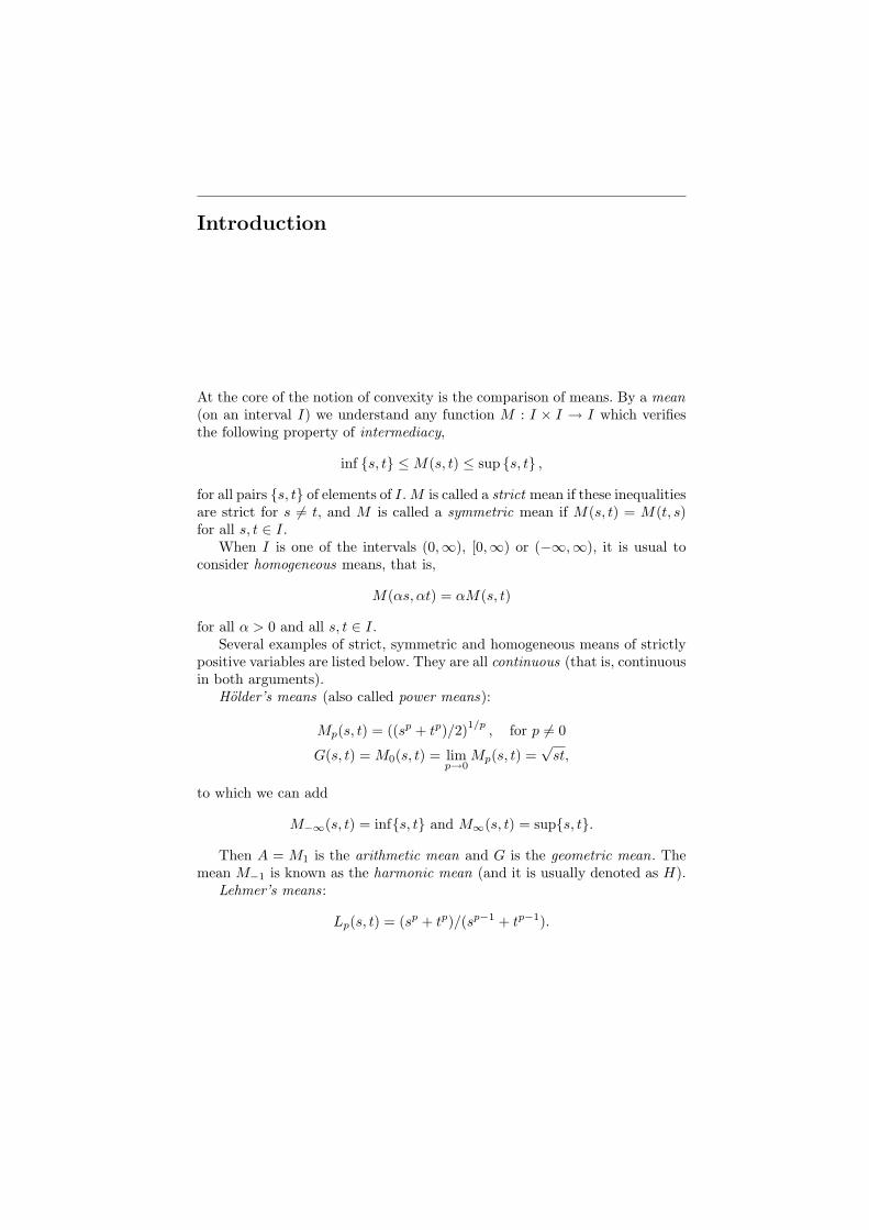
At the core of the notion of convexity is the comparison of means. By a mean(on an interval I) we understand any function M : I × I → I which verifiesthe following property of intermediacy,
inf s, t ≤ M(s, t) ≤ sup s, t ,
for all pairs s, t of elements of I. M is called a strict mean if these inequalitiesare strict for s 6= t, and M is called a symmetric mean if M(s, t) = M(t, s)for all s, t ∈ I.
When I is one of the intervals (0,∞), [0,∞) or (−∞,∞), it is usual toconsider homogeneous means, that is,
M(αs, αt) = αM(s, t)
for all α > 0 and all s, t ∈ I.Several examples of strict, symmetric and homogeneous means of strictly
positive variables are listed below. They are all continuous (that is, continuousin both arguments).
Holder’s means (also called power means):
Mp(s, t) = ((sp + tp)/2)1/p, for p 6= 0
G(s, t) = M0(s, t) = limp→0
Mp(s, t) =√
st,
to which we can add
M−∞(s, t) = infs, t and M∞(s, t) = sups, t.
Then A = M1 is the arithmetic mean and G is the geometric mean. Themean M−1 is known as the harmonic mean (and it is usually denoted as H).
Lehmer’s means:
Lp(s, t) = (sp + tp)/(sp−1 + tp−1).
6 Introduction
Note that L1 = A, L1/2 = G and L0 = H. These are the only means that areboth Lehmer means and Holder means.
Stolarsky’s means:
Sp(s, t) = [(sp − tp)/(ps− pt)]1/(p−1), p 6= 0, 1;
The limiting cases (p = 0 and p = 1) give the logarithmic and identric means,respectively. Thus
S0(s, t) = limp→0
Sp(s, t) =s− t
log s− log t= L(s, t)
S1(s, t) = limp→1
Sp(s, t) =1e
(tt
ss
)1/(t−s)
= I(s, t).
Notice that S2 = A and S−1 = G. The reader may find a comprehensiveaccount on the entire topics of means in [45].
An important mathematical problem is to investigate how functions be-have under the action of means. The most known case is that of midpointconvex (or Jensen convex ) functions, which deal with the arithmetic mean.They are precisely the functions f : I → R such that
f
(x + y
2
)≤ f(x) + f(y)
2(J)
for every x, y ∈ I. In the context of continuity (which appears to be the onlyone of real interest), midpoint convexity means convexity, that is,
f ((1− λ)x + λy) ≤ (1− λ)f(x) + λf(y) (C)
for every x, y ∈ I and every λ ∈ [0, 1]. See Theorem 1.1.4 for details. Bymathematical induction we can extend the inequality (C) to the convex com-binations of finitely many points in I and next to random variables associatedto arbitrary probability spaces. These extensions are known as the discreteJensen inequality and respectively the integral Jensen inequality.
It turns out that similar results work when the arithmetic mean is replacedby any other mean with nice properties. For example, this is the case ofregular means. A mean M : I × I → R is called regular if it is homogeneous,symmetric, continuous and also increasing in each variable (when the otheris fixed). Notice that the Holder means and the Stolarsky means are regular.The Lehmer’s mean L2 is not increasing (and thus it is not regular).
The regular means can be extended from pairs of real numbers to ran-dom variables associated to probability spaces through a process providing anonlinear theory of integration.
Consider first the case of a discrete probability field (X, Σ, µ) , where X =1, 2, Σ = P (1, 2) and µ : P (1, 2) → [0, 1] is the probability measuresuch that µ(i) = λi for i = 1, 2. A random variable associated to this spacewhich takes values in I is any function
Introduction 7
h : 1, 2 → I, h(i) = xi.
The mean M extends to a mean M(h;µ) = M(x1, x2; λ1, λ2), on the setof all such random variables h. In this respect M(x1, x2;λ1, λ2) appears as aweighted mean of x1 and x2 with weights λ1 and λ2 respectively. We startwith the formulas
M(x1, x2; 1, 0) = x1
M(x1, x2; 0, 1) = x2
M(x1, x2; 1/2, 1/2) = M(x1, x2)
and for the other dyadic values of λ1 and λ2 we put
M(x1, x2; 3/4, 1/4) = M(M(x1, x2), x1)M(x1, x2; 1/4, 3/4) = M(M(x1, x2), x2)
and so on. In the general case, every λ1 ∈ [0, 1), has a unique dyadic repre-sentation λ1 =
∑∞k=1 dk/2k (where d1, d2, d3, ... is a sequence consisting of 0
and 1, which is not eventually 1) and we put
M(x1, x2; λ1, λ2) = limn→∞
M
(x1, x2;
n∑
k=1
dk/2k, 1−n∑
k=1
dk/2k
).
Now we can pass to the case of discrete probability spaces built on spaceswith three atoms via the formulas
M(x1, x2, x3;λ1, λ2, λ3) = M
(M
(x1, x2;
λ1
1− λ3,
λ2
1− λ3
), x3; 1− λ3, λ3
).
In the same manner, we can define the means M(x1, . . . , xn; λ1, . . . , λn),associated to random variables on probability spaces having n atoms.
We can bring together all power means Mp, for p ∈ R, by considering theso called quasi-arithmetic means,
M[ϕ] (s, t) = ϕ−1
(12
ϕ(s) +12
ϕ(t))
,
which are associated to strictly monotonic continuous mappings ϕ : I → R;the power mean Mp corresponds to ϕ(x) = xp, if p 6= 0, and to ϕ(x) = log x,if p = 0. For these means,
M[ϕ](x1, ..., xn; λ1, ..., λn) = ϕ−1
(n∑
k=1
λkϕ(xk)
).
Particularly,
A(x1, . . . , xn; λ1, . . . , λn) =n∑
k=1
λkxk,

8 Introduction
in the case of the arithmetic mean, and
G(x1, ..., xn;λ1, ..., λn) =n∏
k=1
xλk
k ,
in the case of the geometric mean.The algorithm described above may lead to very complicated formulas for
the weighted means M(x1, ..., xn; λ1, ..., λn) when M is not a quasi-arithmeticmean. For example, this is the case when M is the logarithmic mean L. How-ever, the weighted means L(x1, ..., xn; λ1, ..., λn) can be introduced by a dif-ferent algorithm proposed by A. O. Pittenger [203]).
We can build a generalized theory of convexity (referred to as the theoryof comparative convexity) simply, by replacing the arithmetic mean by othersmeans. To be more specific, suppose there are given a pair of means M andN on the intervals I and J. A function f : I → J is called (M, N)-midpointaffine, (M, N)-midpoint convex and (M,N)-midpoint concave if, respectively,
f(M(x, y)) = N(f(x), f(y))f(M(x, y)) ≤ N(f(x), f(y))f(M(x, y)) ≥ N(f(x), f(y))
for every x, y ∈ I (see G. Aumann [14]). The condition of midpoint affinity isessentially a functional equation and this explain way the theory of compara-tive convexity has much in common with the subject of functional equations.
While the general theory of comparative convexity is still at infancy, thereare some notable facts to be noted here. For example, an easy inductive ar-gument leads us to the following result:
Theorem A (The discrete form of Jensen’s inequality). If M and N areregular means, and F : I → J is an (M, N)-midpoint convex continuousfunction, then
F (M(x1, ..., xn;λ1, ..., λn)) ≤ N((F (x1), ..., F (xn); λ1, ..., λn))
for every x1, ..., xn ∈ I and every λ1, . . . , λn ∈ [0, 1] with∑n
k=1 λk = 1.
If (X, Σ, µ) is an arbitrary probability field, it is still possible to define themean M(h; µ) for certain real random variables h ∈ L1
R(µ) with values in I.In fact, letting (Σα)α be an upward directed net of finite subfields Σ whoseunion is Σ, the conditional expectation E(F |Σα) of F ∈ L1(µ) with respectto Σα gives rise to a positive contractive projection
Pα : L1(µ) → L1(µ|Σα), Pα(F ) = E(F |Σα),
andE(F |Σα) → F in the norm topology of L1(µ),
by the Lebesgue theorem on dominated convergence. See [104], p. 369.
Introduction 9
A real random variable h ∈ L1R(µ) (with values in I) will be called M -
integrable provided that the limit
M(h; µ) = limα
M(Pα(h); µ|Σα)
exists whenever (Σα)α is an upward directed net of finite subfields of Σ whoseunion generates Σ.
For the quasi-arithmetic mean M[ϕ] (associated to a strictly monotonecontinuous mapping ϕ : I → R) and the probability field associated to therestriction of the Lebesgue measure to an interval [s, t] ⊂ I, the constructionabove yields
M[ϕ]
(id[s,t];
1t− s
dx
)= ϕ−1
(1
t− s
∫ t
s
ϕ(x) dx
),
which coincides with the so called integral ϕ-mean of s and t (also denotedIntϕ (s, t)). Using the fundamental theorem of Calculus, it is easy to see that,on each interval I, the set of all integral means equals the set of all differen-tial means. The differential ψ-mean of s and t (associated to a differentiablemapping ψ : I → R for which ψ′ is one-to-one) is given by the formula
Dψ (s, t) = (ψ′)−1
(ψ(t)− ψ(s)
t− s
).
Passing to the limit in Theorem A we obtain:
Theorem B (The continuous form of Jensen’s inequality). Under the assump-tions of Theorem A, if (X,Σ, µ) is a probability field, then
F (M(h;µ)) ≤ N((F h;µ))
for every h ∈ L1R(µ) such that h is M -integrable and F h is N -integrable.
Theorem C (The Hermite-Hadamard inequality). Suppose that M and Nare regular means and F : I → J is a continuous function. Then F is (M, N)-midpoint convex if and only if for all s < t in I and all probability measuresµ on [s, t] we have the inequality
F (M(s; t)) ≤ N((F |[s,t]; µ)).
Proof. The necessity follows from Theorem B (applied to h = id[s,t]). Thesufficiency represents the particular case where µ = (δs + δt)/2. Here δx
represents the Dirac measure concentrated at x. ¥It is worth to mention the possibility to extend Theorem B beyond the class
of probability measures. That can be done under the additional assumption ofpositive homogeneity (both for the means M and N, and the involved functionF ) following the model of Lebesgue theory, where formulae such as
10 Introduction
∫
Rf(x) dx = lim
n→∞
[2n
(12n
∫ n
−n
f(x) dx
)]
hold. Given a measurable σ-field (X,Σ, µ), a function h : X → R will becalled M -integrable provided the limit
M(h; µ) = limn→∞
[µ(Ωn) ·M
(h|Ωn ;
µ|Σ∩Ωn
µ(Ωn)
)]
exists for every increasing sequence (Ωn)n of elements of Σ with ∪nΩn = X.Then
F (M(h;µ)) ≤ N((F h;µ))
for every h ∈ L1R(µ) such that h is M -integrable and F h is N -integrable (a
fact which extends Theorem C). An illustration of this construction is offeredin Section 3.6.
The theory of comparative convexity encompasses a large variety of classesof convex like functions: the log-convex functions, p-convex functions, quasi-convex functions etc. While it is good to understand what they have in com-mon, it is of equal importance to look inside their own fields.
Chapter 1 is devoted to the case of convex functions on intervals. Wefind there a rich diversity of results with important applications and deepgeneralizations to the context of several variables.
Chapter 2 is aimed to be a specific presentation of other classes of functionsacting on intervals, that verify a condition of (M, N)-convexity. A theory onrelative convexity, built on the concept of convexity of a function with respectto another function, is also included.
The basic theory of convex functions defined on convex sets in a normedlinear space is presented in Chapter 3. The case of functions of several realvariables offers many opportunities to illustrate the depth of the subject ofconvex functions by a number of powerful results: the existence of the or-thogonal projection, the subdifferential calculus,the famous Prekopa-Leindlerinequality (and some of its ramifications), Alexandrov’s beautiful result on thetwice differentiability almost everywhere of a convex function, the solution tothe convex programming problem etc.
Chapter 4 is devoted to Choquet’s theory and its extension to the con-text of Steffensen-Popoviciu measures. This encompasses several remarkableresults such as the Hermite-Hadamard inequality, the Jensen-Steffensen in-equality, Choquet’s integral representation, etc.
As the material on convex functions (and their generalizations) is ex-tremely vast, we had to restrict ourselves to some basic questions, leavinguntouched many subjects which other people will probably consider of ut-most importance. The Comments section at the end of each chapter, and theAppendixes at the end of this book include many results and references tohelp the reader for a better understanding of the field of convex functions.

1
Convex Functions on Intervals
The study of convex functions begins in the context of real-valued functionsof a real variable. Here we find a rich variety of results with significant appli-cations. More important, they will serve as a model for deep generalizationsinto the setting of several variables.
1.1 Convex Functions at a First Glance
Throughout this book I will denote a nondegenerate interval.
1.1.1. Definition. A function f : I → R is called convex if
f((1− λ)x + λy) ≤ (1− λ)f(x) + λf(y) (1.1)
for all points x and y in I and all λ ∈ [0, 1]. It is called strictly convex ifthe inequality (1.1) holds strictly whenever x and y are distinct points andλ ∈ (0, 1). If −f is convex (respectively, strictly convex) then we say that f isconcave (respectively, strictly concave). If f is both convex and concave, thenf is said to be affine.
The affine functions on intervals are precisely the functions of the formmx + n, for suitable constants m and n. One can easily prove that the fol-lowing three functions are convex (though not strictly convex): the positivepart x+, the negative part x−, and the absolute value |x| . Together with theaffine functions they provide the building blocks for the entire class of convexfunctions on intervals. See Theorem 1.5.7.
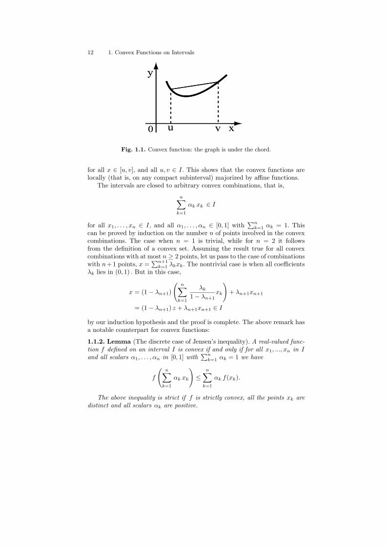
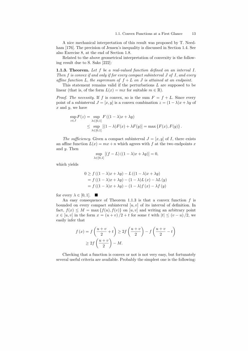
The convexity of a function f : I → R means geometrically that thepoints of the graph of f |[u, v] are under the chord (or on the chord) joiningthe endpoints (u, f(u)) and (v, f(v)), for every u, v ∈ I. See Fig. 1.1. Then
f(x) ≤ f(u) +f(v)− f(u)
v − u(x− u) (1.2)
12 1. Convex Functions on Intervals
Fig. 1.1. Convex function: the graph is under the chord.
for all x ∈ [u, v], and all u, v ∈ I. This shows that the convex functions arelocally (that is, on any compact subinterval) majorized by affine functions.
The intervals are closed to arbitrary convex combinations, that is,
n∑
k=1
αk xk ∈ I
for all x1, . . . , xn ∈ I, and all α1, . . . , αn ∈ [0, 1] with∑n
k=1 αk = 1. Thiscan be proved by induction on the number n of points involved in the convexcombinations. The case when n = 1 is trivial, while for n = 2 it followsfrom the definition of a convex set. Assuming the result true for all convexcombinations with at most n ≥ 2 points, let us pass to the case of combinationswith n+1 points, x =
∑n+1k=1 λkxk. The nontrivial case is when all coefficients
λk lies in (0, 1) . But in this case,
x = (1− λn+1)
(n∑
k=1
λk
1− λn+1xk
)+ λn+1xn+1
= (1− λn+1) z + λn+1xn+1 ∈ I
by our induction hypothesis and the proof is complete. The above remark hasa notable counterpart for convex functions:
1.1.2. Lemma (The discrete case of Jensen’s inequality). A real-valued func-tion f defined on an interval I is convex if and only if for all x1, ..., xn in Iand all scalars α1, . . . , αn in [0, 1] with
∑nk=1 αk = 1 we have
f
(n∑
k=1
αk xk
)≤
n∑
k=1
αk f(xk).
The above inequality is strict if f is strictly convex, all the points xk aredistinct and all scalars αk are positive.
1.1. Convex Functions at a First Glance 13
A nice mechanical interpretation of this result was proposed by T. Need-ham [176]. The precision of Jensen’s inequality is discussed in Section 1.4. Seealso Exercise 8, at the end of Section 1.8.
Related to the above geometrical interpretation of convexity is the follow-ing result due to S. Saks [222]:
1.1.3. Theorem. Let f be a real-valued function defined on an interval I.Then f is convex if and only if for every compact subinterval J of I, and everyaffine function L, the supremum of f + L on J is attained at an endpoint.
This statement remains valid if the perturbations L are supposed to belinear (that is, of the form L(x) = mx for suitable m ∈ R).
Proof. The necessity. If f is convex, so is the sum F = f + L. Since everypoint of a subinterval J = [x, y] is a convex combination z = (1− λ)x + λy ofx and y, we have
supz∈J
F (z) = supλ∈[0,1]
F ((1− λ)x + λy)
≤ supλ∈[0,1]
[(1− λ)F (x) + λF (y)] = max F (x), F (y) .
The sufficiency. Given a compact subinterval J = [x, y] of I, there existsan affine function L(x) = mx + n which agrees with f at the two endpoints xand y. Then
supλ∈[0,1]
[(f − L) ((1− λ)x + λy)] = 0,
which yields
0 ≥ f ((1− λ)x + λy)− L ((1− λ)x + λy)= f ((1− λ)x + λy)− (1− λ)L (x)− λL (y)= f ((1− λ)x + λy)− (1− λ)f (x)− λf (y)
for every λ ∈ [0, 1]. ¥An easy consequence of Theorem 1.1.3 is that a convex function f is
bounded on every compact subinterval [u, v] of its interval of definition. Infact, f(x) ≤ M = max f(u), f(v) on [u, v] and writing an arbitrary pointx ∈ [u, v] in the form x = (u + v) /2 + t for some t with |t| ≤ (v − u) /2, weeasily infer that
f (x) = f
(u + v
2+ t
)≥ 2f
(u + v
2
)− f
(u + v
2− t
)
≥ 2f
(u + v
2
)−M.
Checking that a function is convex or not is not very easy, but fortunatelyseveral useful criteria are available. Probably the simplest one is the following:

14 1. Convex Functions on Intervals
1.1.4. Theorem (J. L. W. V. Jensen [116]). Let f : I → R be a continuousfunction. Then f is convex if and only if f is midpoint convex , that is,
x, y ∈ I implies f
(x + y
2
)≤ f(x) + f(y)
2.
Proof. Clearly, only the sufficiency part needs an argument. By reductio adabsurdum, if f is not convex, then it would exist a subinterval [a, b] such thatthe graph of f |[a, b] is not under the chord joining (a, f(a)) and (b, f(b)), thatis, the function
ϕ(x) = f(x)− f(b)− f(a)b− a
(x− a)− f(a), x ∈ [a, b]
verifies γ = sup ϕ(x) |x ∈ [a, b] > 0. Notice that ϕ is continuous and ϕ(a) =ϕ(b) = 0. Also, a direct computation shows that ϕ is also midpoint convex.Put c = inf x ∈ [a, b] |ϕ(x) = γ ; then necessarily ϕ(c) = γ and c ∈ (a, b).By the definition of c, for every h > 0 for which c± h ∈ (a, b) we have
ϕ(c− h) < ϕ(c) and ϕ(c + h) ≤ ϕ(c)
so that
ϕ(c) >ϕ(c− h) + ϕ(c + h)
2in contradiction with the fact that ϕ is midpoint convex. ¥1.1.5. Corollary. Let f : I → R be a continuous function. Then f is convexif and only if
f(x + h) + f(x− h)− 2f(x) ≥ 0
for all x ∈ I and all h > 0 such that both x + h and x− h are in I.Notice that both Theorem 1.1.4 and its Corollary 1.1.5 above have straight-
forward variants for the case of strictly convex functions.Corollary 1.1.5 allows us to check immediately the strict convexity of some
very common functions such as the exponential function. In fact, due to thefact that
a, b > 0, a 6= b, impliesa + b
2>√
ab
we haveex+h + ex−h − 2 ex > 0
for all x ∈ R and all h > 0.An immediate consequence of the strict convexity of exp is the following
result, which extends the famous arithmetic mean-geometric mean inequality(abbreviated, AM −GM inequality):1.1.6. Theorem (The weighted form of the AM − GM inequality; L. J.Rogers [218]). If x1, ..., xn ∈ (0,∞) and α1, ..., αn ∈ (0, 1),
∑nk=1 αk = 1,
then

1.1. Convex Functions at a First Glance 15
n∑
k=1
αkxk > xα11 · · ·xαn
n
unless x1 = ... = xn.
Replacing xk by 1/xk in the last inequality we get (under the same hy-potheses on xk and αk),
xα11 · · ·xαn
n > 1 /
n∑
k = 1
αk
xk
unless x1 = ... = xn (which represents the weighted form of the geometricmean-harmonic mean inequality).
The particular case of the Theorem 1.1.6 where α1 = ... = αn = 1/nrepresents the usual AM −GM inequality , which can be completed as above,with its relation to the harmonic mean: For every family x1, ..., xn of positivenumbers we have
x1 + · · ·+ xn
n> n√
x1 · · ·xn > n/
(1x1
+ · · ·+ 1xn
)
unless x1 = ... = xn. An estimate of these inequalities makes the object ofSection 2.5 below.
The permanence properties of convexity operations with convex functionsconstitute an important source of examples in this area:1.1.7. Proposition (The operations with convex functions).
i) Adding two convex functions (defined on the same interval) we obtain aconvex function; if one of them is strictly convex then the sum is also strictlyconvex.
ii) Multiplying a (strictly) convex function by a positive scalar we obtainalso a (strictly) convex function.
iii) The restriction of every (strictly) convex function to a subinterval ofits domain is also a (strictly) convex function.
iv) If f : I → R is a convex (respectively a strictly convex ) function andg : R→ R is a nondecreasing (respectively an increasing) convex function,then g f is convex (respectively strictly convex ).
v) Suppose that f is a bijection between two intervals I and J. If f isincreasing, then f is (strictly) convex if and only if f−1 is (strictly) concave.
If f is a decreasing bijection, then f and f−1 are of the same type ofconvexity.
We end this section with a result related to Theorem 1.1.4:
1.1.8. Theorem (Popoviciu’s inequality [209]). Let f : I → R be a continuousfunction. Then f is convex if and only if
f(x) + f(y) + f(z)3
+ f
(x + y + z
3
)≥
16 1. Convex Functions on Intervals
≥ 23
[f
(x + y
2
)+ f
(y + z
2
)+ f
(z + x
2
)]
for all x, y, z ∈ I.In the variant of strictly convex functions the above inequality is strict
except for x = y = z.
Proof. The Necessity (This implication needs not the assumption on con-tinuity). Without loss of generality we may assume that x ≤ y ≤ z. Ify ≤ (x + y + z) /3 , then
(x + y + z) /3 ≤ (x + z) /2 ≤ z and (x + y + z) /3 ≤ (y + z) /2 ≤ z,
which yields two numbers s, t ∈ [0, 1] such that
x + z
2= s · x + y + z
3+ (1− s) · z
y + z
2= t · x + y + z
3+ (1− t) · z.
Summing up, we get (x + y − 2z) (s + t− 3/2) = 0. If x + y − 2z = 0, thennecessarily x = y = z, and Popoviciu’s inequality is clear.
If s + t = 3/2, we have to sum up the following three inequalities
f
(x + z
2
)≤ s · f
(x + y + z
3
)+ (1− s) · f(z)
f
(y + z
2
)≤ t · f
(x + y + z
3
)+ (1− t) · f(z)
f
(x + y
2
)≤ 1
2· f(x) +
12· f(y)
and then to multiply both sides by 2/3.The case where (x + y + z) /3 < y can be treated in a similar way.The Sufficiency. Popoviciu’s inequality (when applied for y = z), yields
the following substitute for the condition of midpoint convexity:
14f(x) +
34f
(x + 2y
3
)≥ f
(x + y
2
)for all x, y ∈ I, (1.3)
Using this remark, the proof follows verbatim the argument of Theorem 1.1.4above. ¥
The above statement of Popoviciu’s inequality is only a simplified ver-sion of a considerably more general result. See the Comments at the end ofthis chapter. However, even this version leads to interesting inequalities. SeeExercise 9. As estimate from below of Popoviciu’s inequality is available in[191].

1.1. Convex Functions at a First Glance 17
Exercises
1. Prove that the following functions are strictly convex:− log x and x log x on (0,∞);xp on [0,∞) if p > 1; xp on (0,∞) if p < 0; −xp on [0,∞) if p ∈ (0, 1);(1 + xp)1/p on [0,∞) if p > 1.
2. Let f : I → R be a convex function and let x1, ..., xn ∈ I (n ≥ 2). Provethat
(n− 1)[f(x1) + · · ·+ f(xn−1)
n− 1− f
(x1 + · · ·+ xn−1
n− 1
)]
cannot exceed
n
[f(x1) + · · ·+ f(xn)
n− f
(x1 + · · ·+ xn
n
)].
3. Let x1, ..., xn > 0 (n ≥ 2) and for each 1 ≤ k ≤ n put
Ak =x1 + · · ·+ xk
kand Gk = (x1 · · ·xk)1/k
.
i) (T. Popoviciu). Prove that
(An
Gn
)n
≥(
An−1
Gn−1
)n−1
≥ · · · ≥(
A1
G1
)1
= 1.
ii) (T. Rado). Prove that
n(An −Gn) ≥ (n− 1)(An−1 −Gn−1) ≥ · · · ≥ 1 · (A1 −G1) = 0.
[Hint : Apply the result of Exercise 2 to f = − log and respectively tof = exp . ]
4. Suppose that f1, ..., fn are nonnegative convex functions with the samedomain of definition. Prove that (f1 · · · fn)1/n is also a convex function.
5. i) Prove that Theorem 1.1.4 remains true if the condition of midpointconvexity is replaced by f ((1− α)x + αy) ≤ (1 − α)f(x) + αf(y), forsome fixed parameter α ∈ (0, 1).ii) Prove that Theorem 1.1.4 remains true if the condition of continuity isreplaced by boundedness from above on every compact subinterval.
6. (New from old). Assume that f(x) is a (strictly) convex function for x > 0.Prove that xf(1/x) is (strictly) convex too.
7. Infer from Theorem 1.1.6 that minx,y>0
(x + y + 1
x2y
)= 4/
√2.
8. (The power means in the discrete case. See Section 1.8, Exercise 1, for theintegral case). Let x = (x1, . . . , xn) and α = (α1, . . . , αn) be two n-tuplesof strictly positive elements, such that
∑nk=1 αk = 1. The (weighted) power
mean of order t is defined as
18 1. Convex Functions on Intervals
Mt(x; α) =
(n∑
k=1
αkxtk
)1/t
for t 6= 0
and
M0(x;α) = limt→ 0+
Mt(x, α) =n∏
k = 1
xαk
k .
Notice that M1 is the arithmetic mean, M0 is the geometric mean andM−1 is the harmonic mean.i) Apply Jensen’s inequality to the function xt/s, to prove that
s ≤ t implies Ms(x; α) ≤ Mt(x;α).
ii) Prove that the function t → t log Mt(x; α) is convex on R.iii) We define M−∞(x;α) = inf xk | k and M∞(x, α) = sup xk | k .Prove that
limt→−∞
Mt(x; α) = M−∞(x; α) and limt→∞
Mt(x;α) = M∞(x; α).
9. (An illustration of Popoviciu’s inequality). Suppose that x1, x2, x3 arepositive numbers, not all equal. Prove that:i) 27
∏i<j (xi + xj)
2> 64x1x2x3 (x1 + x2 + x3)
3 ;ii) x6
1 + x62 + x6
3 + 3x21x
22x
23 > 2(x3
1x32 + x3
2x33 + x3
3x31).
1.2 Young’s Inequality and its Consequences
Young’s inequality asserts that
ab ≤ ap
p+
bq
qfor all a, b ≥ 0,
whenever p, q ∈ (1,∞) and 1/p + 1/q = 1; the equality holds if (and onlyif) ap = bq. This is a consequence of the strict convexity of the exponentialfunction. In fact,
ab = elog ab = e(1/p) log ap+(1/q) log bq
<1p
elog ap
+1q
elog bq
=ap
p+
bq
q
for all a, b > 0 with ap 6= bq. An alternative argument can be obtained bystudying the variation of the function
F (a) =ap
p+
bq
q− ab, a ≥ 0,
where b ≥ 0 is a parameter. F has a strict global minimum at a = bq/p, whichyields F (a) > F (bq/p) = 0 for every a ≥ 0, a 6= bq/p.

1.2. Young’s Inequality and its Consequences 19
W. H. Young [249] proved actually a much more general inequality whichyields the aforementioned one for f(x) = xp−1 :
1.2.1. Theorem (Young’s inequality). Suppose that f : [0,∞) → [0,∞) isan increasing continuous function such that f(0) = 0 and limx→∞ f(x) = ∞.Then
ab ≤∫ a
0
f(x) dx +∫ b
0
f−1(x) dx
for every a, b ≥ 0, and equality occurs if and only if b = f(a).Proof. Using the definition of the derivative we can easily prove that thefunction
F (x) =∫ x
0
f(t) dt +∫ f(x)
0
f−1(t) dt− xf(x)
is differentiable, with F ′ identically 0. This yields
0 ≤ u ≤ a and 0 ≤ v ≤ f(a) ⇒ uv ≤∫ u
0
f(t) dt +∫ v
0
f−1(t) dt
and the conclusion of the theorem is now clear. ¥
Fig. 1.2. The areas of the two curvilinear triangles exceed the area of the rectanglewith sides u and v.
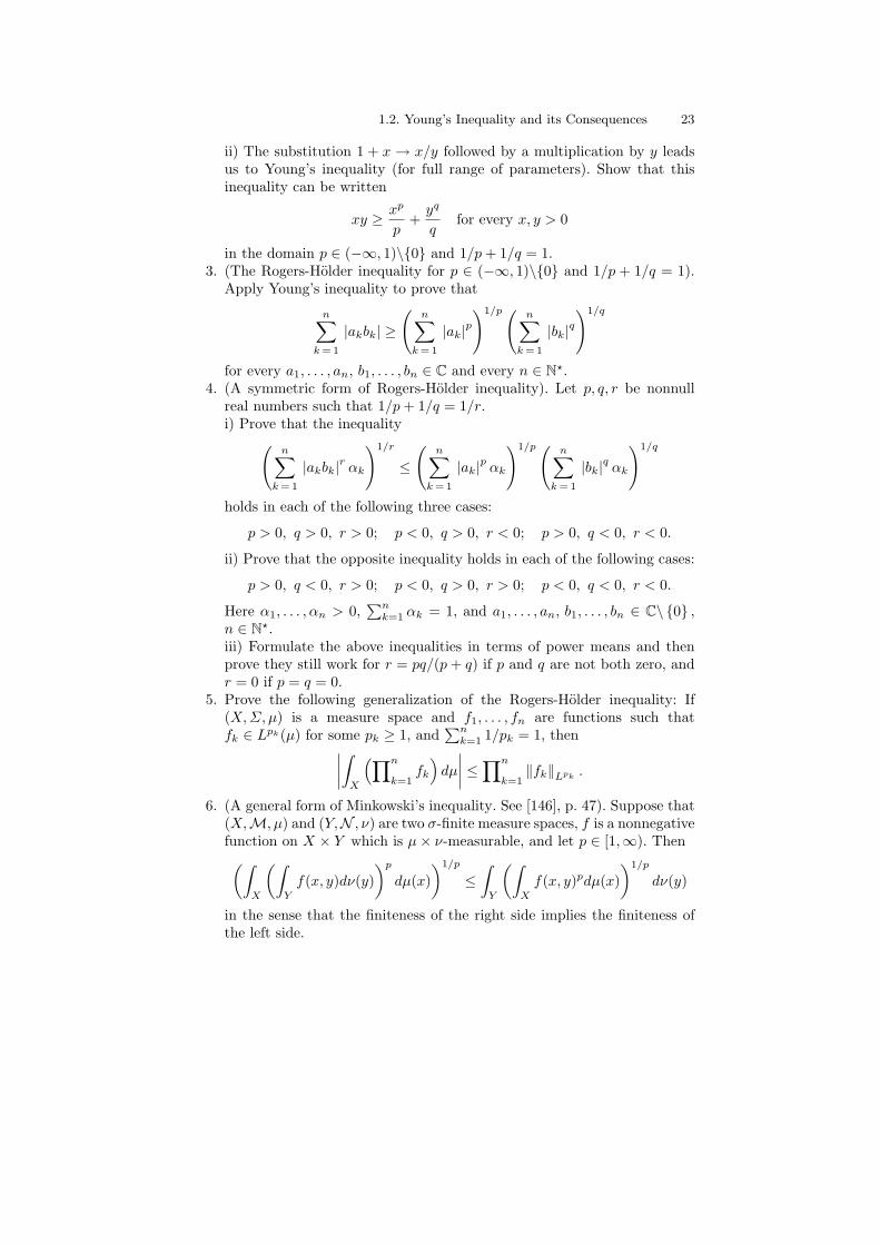
The geometric meaning of Young’s inequality is indicated in Fig. 1.2.Young’s inequality is the source of many basic inequalities. The next two
applications concerns complex functions defined on an arbitrary measure space(X, Σ, µ).1.2.2. Theorem (The Rogers-Holder inequality for p > 1). Let p, q ∈ (1,∞)with 1/p + 1/q = 1, and let f ∈ Lp(µ) and g ∈ Lq(µ). Then fg is in L1(µ)and we have ∣∣∣∣
∫
X
fg dµ
∣∣∣∣ ≤∫
X
|fg| dµ (1.4)
and ∫
X
|fg| dµ ≤ ‖f‖Lp ‖g‖Lq (1.5)

20 1. Convex Functions on Intervals
and thus ∣∣∣∣∫
X
fg dµ
∣∣∣∣ ≤ ‖f‖Lp ‖g‖Lq . (1.6)
The above result extends in a straightforward manner for the pairs p = 1,q = ∞ and p = ∞, q = 1. In the complementary domain, p ∈ (−∞, 1)\0and 1/p + 1/q = 1, the inequality sign in (1.4)-(1.6) should be reversed. SeeExercises 3 and 4.
For p = q = 2, the inequality (1.6) is called the Cauchy-Buniakovski-Schwarz inequality .
Proof. The first inequality is trivial. If f or g is zero µ-almost everywhere,then the second inequality is trivial. Otherwise, using Young’s inequality, wehave
|f(x)|‖f‖Lp
· |g(x)|‖g‖Lq
≤ 1p· |f(x)|p‖f‖p
Lp
+1q· |g(x)|q‖g‖q
Lq
for all x in X, such that fg ∈ L1(µ). Thus
1‖f‖Lp ‖g‖Lq
∫
X
|fg| dµ ≤ 1
and this proves (1.5). The inequality (1.6) is immediate. ¥1.2.3. Remark (Conditions for equality in Theorem 1.2.2). The basic obser-vation is the fact that
f ≥ 0 and∫
X
f dµ = 0 imply f = 0 µ-almost everywhere.
Consequently we have equality in (1.4) if and only if
f(x)g(x) = eiθ |f(x)g(x)|
for some real constant θ and for µ-almost every x.Suppose that p, q ∈ (1,∞). In order to get equality in (1.5) it is necessary
and sufficient to have
|f(x)|‖f‖Lp
· |g(x)|‖g‖Lq
=1p· |f(x)|p‖f‖p
Lp
+1q· |g(x)|q‖g‖q
Lq
almost everywhere. The equality case in Young’s inequality shows that this isequivalent to |f(x)|p / ‖f‖p
Lp = |g(x)|q / ‖g‖qLq almost everywhere, that is,
A |f(x)|p = B |g(x)|q almost everywhere
for some nonnegative numbers A and B.If p = 1 and q = ∞, we have equality in (1.5) if and only if there is a
constant λ ≥ 0 such that |g(x)| ≤ λ almost everywhere, and |g(x)| = λ foralmost every point where f(x) 6= 0.

1.2. Young’s Inequality and its Consequences 21
1.2.4. Theorem (Minkowski’s inequality). For 1 ≤ p < ∞ and f, g ∈ Lp(µ)we have
||f + g||Lp ≤ ||f ||Lp + ||g||Lp . (1.7)
In the discrete case, using the notation of Exercise 8, Section 1.1, thisinequality reads
Mp(x + y, α) ≤ Mp(x, α) + Mp(y, α). (1.8)
In this form, it extends to the complementary range 0 < p < 1, with theinequality sign reversed. The integral analogue for p < 1 is presented in Section3.6.
Proof. For p = 1, the inequality (1.7) follows immediately from |f + g| ≤|f |+ |g|. For p ∈ (1,∞) we have
|f + g|p ≤ (|f |+ |g|)p ≤ (2 sup |f | , |g|)p
≤ 2p (|f |p + |g|p) ,
which shows that f + g ∈ Lp(µ). Moreover, according to Theorem 1.2.2,
||f + g||pLp =∫
X
|f + g|p dµ ≤∫
X
|f + g|p−1 |f | dµ +∫
X
|f + g|p−1 |g| dµ
≤(∫
X
|f |p dµ
)1/p (∫
X
|f + g|(p−1)qdµ
)1/q
+
+(∫
X
|g|p dµ
)1/p (∫
X
|f + g|(p−1)qdµ
)1/q
= (||f ||Lp + ||g||Lp) ||f + g||p/qLp ,
where 1/p + 1/q = 1, and it remains to observe that p− p/q = 1. ¥1.2.5. Remark. If p = 1, we obtain equality in (1.7) if and only if there is apositive measurable function ϕ such that
f(x)ϕ(x) = g(x)
almost everywhere on the set x | f(x)g(x) 6= 0.If p ∈ (1,∞) and f is not 0 almost everywhere, then we have equality in
(1.7) if and only if g = λf almost everywhere, for some λ ≥ 0.
In the particular case when (X, Σ, µ) is the measure space associated withthe counting measure on a finite set,
µ : P(1, ..., n → [0, 1], µ(A) = |A|,
we retrieve the classical discrete forms of the above inequalities. For example,the discrete version of the Rogers-Holder inequality can be read
22 1. Convex Functions on Intervals
∣∣∣∣∣n∑
k = 1
ξkηk
∣∣∣∣∣ ≤(
n∑
k = 1
|ξk|p)1/p (
n∑
k = 1
|ηk|q)1/q
for every ξk, ηk ∈ C, k ∈ 1, ..., n. On the other hand, a moment’s reflectionshows that we can pass immediately from these discrete inequalities to theirintegral analogues, corresponding to finite measure spaces.
1.2.6. Remark. It is important to notice that all numerical inequalities ofthe form
f(x1, ..., xn) ≥ 0 for x1, ..., xn ≥ 0 (1.9)
where f is a continuous and positively homogeneous function of degree 1 (thatis, f(λx1, ..., λxn) = λf(x1, ..., xn) for λ ≥ 0), extend to the context of Banachlattices, via a functional calculus invented by A. J. Yudin and J. L. Krivine.This allows us to replace the real variables of f by positive elements of aBanach lattice. See [149], vol. 2, pp. 40-43. Particularly, this is the case ofAM −GM inequality, Rogers-Holder’s inequality, Minkowski’s inequality etc.
Also, all numerical inequalities of the form (1.9), attached to continuousfunctions, extend (via the functional calculus with self-adjoint elements) to thecontext of C?-algebras. In fact, the n-tuples of real numbers can be replacedby n-tuples of mutually commuting positive elements of a C?-algebra. See[59].
Exercises
1. Recall the identity of Lagrange,(
n∑
k = 1
a2k
)(n∑
k = 1
b2k
)=
∑
1≤j < k≤n
(ajbk − akbj)2 +
(n∑
k = 1
akbk
)2
,
which works for every ak, bk ∈ R, k ∈ 1, ..., n. Infer from it the discreteform of Cauchy-Buniakovski-Schwarz inequality,
∣∣∣∣∣n∑
k = 1
ξkηk
∣∣∣∣∣ ≤(
n∑
k = 1
|ξk|2)1/2 (
n∑
k = 1
|ηk|2)1/2
,
and settle the equality case (in the context of families of complex num-bers).
2. (The Bernoulli inequality). i) Prove that for all x > −1 we have
(1 + x)α ≥ 1 + αx if α ∈ (−∞, 0] ∪ [1,∞)
and(1 + x)α ≤ 1 + αx if α ∈ [0, 1];
if α /∈ 0, 1 , the equality occurs only for x = 0.
1.2. Young’s Inequality and its Consequences 23
ii) The substitution 1 + x → x/y followed by a multiplication by y leadsus to Young’s inequality (for full range of parameters). Show that thisinequality can be written
xy ≥ xp
p+
yq
qfor every x, y > 0
in the domain p ∈ (−∞, 1)\0 and 1/p + 1/q = 1.3. (The Rogers-Holder inequality for p ∈ (−∞, 1)\0 and 1/p + 1/q = 1).
Apply Young’s inequality to prove that
n∑
k = 1
|akbk| ≥(
n∑
k = 1
|ak|p)1/p (
n∑
k = 1
|bk|q)1/q
for every a1, . . . , an, b1, . . . , bn ∈ C and every n ∈ N?.4. (A symmetric form of Rogers-Holder inequality). Let p, q, r be nonnull
real numbers such that 1/p + 1/q = 1/r.i) Prove that the inequality
(n∑
k = 1
|akbk|r αk
)1/r
≤(
n∑
k = 1
|ak|p αk
)1/p (n∑
k = 1
|bk|q αk
)1/q
holds in each of the following three cases:
p > 0, q > 0, r > 0; p < 0, q > 0, r < 0; p > 0, q < 0, r < 0.
ii) Prove that the opposite inequality holds in each of the following cases:
p > 0, q < 0, r > 0; p < 0, q > 0, r > 0; p < 0, q < 0, r < 0.
Here α1, . . . , αn > 0,∑n
k=1 αk = 1, and a1, . . . , an, b1, . . . , bn ∈ C\ 0 ,n ∈ N?.iii) Formulate the above inequalities in terms of power means and thenprove they still work for r = pq/(p + q) if p and q are not both zero, andr = 0 if p = q = 0.
5. Prove the following generalization of the Rogers-Holder inequality: If(X,Σ, µ) is a measure space and f1, . . . , fn are functions such thatfk ∈ Lpk(µ) for some pk ≥ 1, and
∑nk=1 1/pk = 1, then
∣∣∣∣∫
X
(∏n
k=1fk
)dµ
∣∣∣∣ ≤∏n
k=1‖fk‖Lpk .
6. (A general form of Minkowski’s inequality. See [146], p. 47). Suppose that(X,M, µ) and (Y,N , ν) are two σ-finite measure spaces, f is a nonnegativefunction on X × Y which is µ× ν-measurable, and let p ∈ [1,∞). Then(∫
X
(∫
Y
f(x, y)dν(y))p
dµ(x))1/p
≤∫
Y
(∫
X
f(x, y)pdµ(x))1/p
dν(y)
in the sense that the finiteness of the right side implies the finiteness ofthe left side.

24 1. Convex Functions on Intervals
1.3 Smoothness Properties
The entire discussion on the smoothness properties of convex functions onintervals is based on their characterization in terms of slopes of variable secantsthrough arbitrary fixed points of their graphs.
Given a function f : I → R and a point a ∈ I, one can associate to thema new function,
sa : I \ a → R, sa(x) =f(x)− f(a)
x− a,
whose value at x is the slope of the secant joining the points (a, f(a)) and(x, f(x)) of the graph of f.
1.3.1. Theorem (L. Galvani [87]). Let f be a real function defined on aninterval I. Then f is convex (respectively strictly convex ) if and only if theassociated functions sa are nondecreasing (respectively increasing).
In fact,
sa(y)− sa(x)y − x
=
∣∣∣∣∣∣
1 x f(x)1 y f(y)1 a f(a)
∣∣∣∣∣∣
/∣∣∣∣∣∣
1 x x2
1 y y2
1 a a2
∣∣∣∣∣∣for all three distinct points a, x, y of I, and the proof of Theorem 1.3.1 is aconsequence of the following lemma:
1.3.2. Lemma. Let f be a real function defined on an interval I. Then f isconvex if and only if
∣∣∣∣∣∣
1 x f(x)1 y f(y)1 z f(z)
∣∣∣∣∣∣
/∣∣∣∣∣∣
1 x x2
1 y y2
1 z z2
∣∣∣∣∣∣≥ 0
for all three distinct points x, y, z of I; equivalently, if and only if∣∣∣∣∣∣
1 x f(x)1 y f(y)1 z f(z)
∣∣∣∣∣∣≥ 0 (1.10)
for all x < y < z in I.The corresponding variant for strict convexity is valid too, provided that
≥ is replaced by > .
Proof. The condition (1.10) means that
(z − y) f(x)− (z − x) f(y) + (y − x) f(z) ≥ 0
for all x < y < z in I. Since each y between x and z can be written asy = (1− λ)x + λz, the latter condition is equivalent to the assertion that

1.3. Smoothness Properties 25
f ((1− λ)x + λz) ≤ (1− λ) f(x) + λ f(z)
for all x < z in I and all λ ∈ [0, 1]. ¥We are now prepared to state the main result on the smoothness of convex
functions.1.3.3. Theorem (O. Stolz [237]). Let f : I → R be a convex function.Then f is continuous on the interior int I of I and has finite left and rightderivatives at each point of int I. Moreover, x < y in int I implies
f ′−(x) ≤ f ′+(x) ≤ f ′−(y) ≤ f ′+(y)
Particularly, both f ′− and f ′+ are nondecreasing on int I.Proof. In fact, according to Theorem 1.3.1 above, we have
f(x)− f(a)x− a
≤ f(y)− f(a)y − a
≤ f(z)− f(a)z − a
for all x ≤ y < a < z in I. This fact assures us that the left derivative at aexists and
f ′−(a) ≤ f(z)− f(a)z − a
.
A symmetric argument will then yield the existence of f ′+(a) and theavailability of the relation f ′−(a) ≤ f ′+(a). On the other hand, starting withx < u ≤ v < y in int I, the same Theorem 1.3.1 yields
f(u)− f(x)u− x
≤ f(v)− f(x)v − x
≤ f(v)− f(y)v − y
so, letting u → x+ and v → y−, we obtain that f ′+(x) ≤ f ′−(y).Because f admits finite lateral derivatives at each interior point, it will be
continuous at each interior point. ¥By Theorem 1.3.3, every continuous convex function f (defined on a non-
degenerate compact interval [a, b]) admits derivatives f ′+(a) and f ′(b) at theendpoints, but they can be infinite,
−∞ ≤ f ′+(a) < ∞ and −∞ < f ′(b) ≤ ∞.
How nondifferentiable can a convex function be? Due to Theorem 1.3.3above we can immediately prove that every convex function f : I → R isdifferentiable except for an enumerable subset. In fact, by considering the set
Ind = x | f ′−(x) < f ′+(x)
and letting for each x ∈ Ind a rational point rx ∈(f ′−(x), f ′+(x)
)we get an
one-to-one function ϕ : x → rx from Ind into Q. Consequently, Ind is at mostcountable. Notice that this reasoning depends on the Axiom of choice.
26 1. Convex Functions on Intervals
An example of a convex function which is not differentiable on a densecountable set will be exhibited in Remark 1.6.2 below. See also Exercise 1 atthe end of this section.
Simple examples such as f(x) = 0 if x ∈ (0, 1), and f(0) = f(1) = 1, showthat at the endpoints of the interval of definition of a convex function couldappear upward jumps. Fortunately, the possible discontinuities are removable:1.3.4. Proposition. If f : [a, b] → R is a convex function, then f(a+) andf(b−) exist in R and
f(x) =
f(a+) if x = af(x) if x ∈ (a, b)f(b−) if x = b
is convex too.
This result is a consequence of the following:1.3.5. Proposition. If f : I → R is convex, then either f is monotonic onint I, or there exists an ξ ∈ int I such that f is nonincreasing on the interval(−∞, ξ] ∩ I and nondecreasing on the interval [ξ,∞) ∩ I.
Proof. Since any convex function verifies formulas of the type (1.2), it sufficesto consider the case where I is open. If f is not monotonic, then there mustexist points a < b < c in I such that
f(a) > f(b) < f(c);
the other possibility, f(a) < f(b) > f(c), is rejected by the same Theorem1.1.3. Since f is continuous on [a, c], it attains its infimum on this interval ata point ξ ∈ [a, c], that is,
f(ξ) = inf f([a, c]).
Actually f(ξ) = inf f(I). In fact, if x < a, then according to Theorem1.3.1 we have
f(x)− f(ξ)x− ξ
≤ f(a)− f(ξ)a− ξ
,
which yields (ξ − a) f(x) ≥ (x− a)f(ξ) + (ξ − x)f(a) ≥ (ξ − a) f(ξ), that is,f(x) ≥ f(ξ). The other case, when c < x, can be treated in a similar manner.
If u < v < ξ, then
su(ξ) = sξ(u) ≤ sξ(v) =f(v)− f(ξ)
v − ξ≤ 0
and thus su(v) ≤ su(ξ) ≤ 0. This yields that f is nonincreasing on I∩(−∞, ξ].Analogously, if ξ < u < v, then from sv(ξ) ≤ sv(u) we infer that f(v) ≥ f(u),that is, f is nondecreasing on I ∩ [ξ,∞). ¥

1.3. Smoothness Properties 27
1.3.6. Corollary. Every convex function f : I → R which is not monotonicon int I has an interior global minimum.
There is another way to look at the smoothness properties of the convexfunctions, based on the Lipschitz condition. A function f defined on an intervalJ is said to be Lipschitz if there exists a constant L ≥ 0 such that
|f(x)− f(y)| ≤ L |x− y| for all x, y ∈ J.
A famous result due to H. Rademacher asserts that any Lipschitz functionis differentiable almost everywhere. See Section 3.11.1.3.7. Theorem. If f : I → R is a convex function, then f is Lipschitz onany compact interval [a, b] contained in the interior of I.
Proof. Choose ε > 0 such that a− ε and b + ε belong to I, and let m and Mbe the lower and upper bounds of f on [a− ε, b + ε] . If x and y are distinctpoints of [a, b], put z = y + ε (y − x) / |y − x| . Then z ∈ [a− ε, b + ε] and
y = (1− λ)z + λx for λ =ε
ε + |y − x| .
Therefore f(y) ≤ (1− λ)f(z) + λf(x), which yields
f(y)− f(x) ≤ (1− λ)(M −m) ≤ M −m
ε|y − x| .
Since this is true for all x, y ∈ [a, b], we conclude that f(y)−f(x) ≤ L |y − x| ,where L = (M −m) /ε. ¥1.3.8. Corollary. If fn : I → R (n ∈ N) is a pointwise converging sequenceof convex functions, then its limit f is also convex. Moreover, the convergenceis uniform on any compact subinterval included in int I.
Since the first derivative of a convex function may not exist at a densesubset, a characterization of convexity in terms of second order derivatives isnot possible unless we relax the concept of twice differentiability. The upperand the lower second symmetric derivative of f at x, are respectively definedby the formulas
D2f(x) = lim sup
h ↓ 0
f(x + h) + f(x− h)− 2f(x)h2
D2f(x) = lim infh ↓ 0
f(x + h) + f(x− h)− 2f(x)h2
.
It is not difficult to check that if f is twice differentiable at a point x, then
D2f(x) = D2f(x) = f ′′(x);
however D2f(x) and D2f(x) can exist even at points of discontinuity; for
example, consider the case of the signum function and the point x = 0.
28 1. Convex Functions on Intervals
1.3.9. Theorem. Suppose that I is an open interval. A real-valued functionf is convex on I if and only if f is continuous and D2
f ≥ 0.According to this result, if a function f : I → R is convex in the neighbor-
hood of each point of I, then it is convex on the whole interval I.
Proof. If f is convex, then clearly D2f ≥ D2f ≥ 0. The continuity of f follows
from Theorem 1.3.3.Now, suppose that D2
f > 0 on I. If f is not convex, then we can finda point x0 such that D2
f(x0) ≤ 0, which will be a contradiction. In fact, inthis case there exists a subinterval I0 = [a0, b0] such that f((a0 + b0)/2) >(f(a0) + f(b0)) /2. A moment’s reflection shows that one of the intervals[a, (a + b)/2], [(3a + b)/4, (a + 3b)/4], [(a + b)/2, b] can be chosen to re-place I0 by a smaller interval I1 = [a1, b1], with b1 − a1 = (b − a)/2 andf((a1 + b1)/2) > (f(a1) + f(b1)) /2. Proceeding by induction, we arrive at asituation where the principle of included intervals gives us the point x0.
In the general case, consider the sequence of functions
fn(x) = f(x) +1n
x2.
Then D2fn > 0, and the above reasoning shows us that fn is convex. Clearly
fn(x) → f(x) for each x ∈ I, so that the convexity of f will be a consequenceof Corollary 1.3.8 above. ¥1.3.10. Corollary. Suppose that f : I → R is a twice differentiable function.Then:
i) f is convex if and only if f ′′ ≥ 0.ii) f is strictly convex if and only if f ′′ ≥ 0 and the set of points where
f ′′ vanishes does not include intervals of positive length.
An important result due to A. D. Alexandrov asserts that all convex func-tions are almost everywhere twice differentiable. See Section 3.11.1.3.11. Remark (Higher order convexity). The following generalization ofthe notion of a convex function was initiated by T. Popoviciu in 1934. Afunction f : [a, b] → R is said to be n-convex (n ∈ N?) if for all choices ofn + 1 distinct points x0 < · · · < xn in [a, b], the nth order divided differenceof f verifies
f [x0, . . . , xn] ≥ 0.
The divided differences are given inductively by
f [x0, x1] =f(x0)− f(x1)
x0 − x1
f [x0, x1, x2] =f [x0, x1]− f [x1, x2]
x 0 − x2
. . .
f [x0, . . . , xn] =f [x0, . . . , xn−1]− f [x1, . . . , xn]
x 0 − xn.
1.3. Smoothness Properties 29
Thus the 1-convex functions are the nondecreasing functions, while the2-convex functions are precisely the classical convex functions. In fact,
∣∣∣∣∣∣
1 x f(x)1 y f(y)1 z f(z)
∣∣∣∣∣∣/
∣∣∣∣∣∣
1 x x2
1 y y2
1 z z2
∣∣∣∣∣∣=
f [y, z]− f [x, z]y − x
,
and the claim follows from Lemma 1.3.2. As T. Popoviciu noticed in his book[208], if f is n times differentiable, with f (n) ≥ 0, then f is n-convex.
See [198] and [215] for a more detailed account on the theory of n-convexfunctions.
Exercises
1. (An application of the second derivative test of convexity).i) Prove that the functions log ((eax − 1) / (ex − 1)) and log (sinh ax/ sinhx)are convex on R if a ≥ 1.
i) Prove that the function b log cos(x/√
b)−a log cos (x/
√a) is convex on
(0, π/2) if b ≥ a ≥ 1.2. Suppose that 0 < a < b < c (or, 0 < b < c < a or, 0 < c < b < a). Use
Lemma 1.3.2 to infer the following inequalities:i) a
√c + b
√a + c
√b > a
√b + b
√c + c
√a;
ii) abn + bcn + can > acn + ban + cbn (n ≥ 1);iii) abbcca > accbba;iv) a(c−b)
(c+b)(2a+b+c) + b(a−c)(a+c)(a+2b+c) + c(b−a)
(b+a)(a+b+2c) > 0.
3. Show that the function f(x) =∑∞
n = 0 |x − n|/2n, x ∈ R, provides anexample of a convex function which is nondifferentiable on a countablesubset.
4. Let D be a bounded closed convex subset of the real plane. Prove that Dcan be always represented as
D = (x, y) | f(x) ≤ y ≤ g(x), x ∈ [a, b]
for suitable functions f : [a, b] → R convex and g : [a, b] → R concave.Infer that the boundary of D is smooth except for an enumerable subset.
5. Prove that a continuous convex function f : [a, b] → R can be extendedto a convex function on R if and only if f ′+(a) and f ′−(b) are finite.
6. Use Corollary 1.3.10 to prove that the sine function is strictly concave on[0, π]. Infer that
(sin a
a
)x ≤ sin x ≤ sin a
(x
a
)a cot a
for every a ∈ (0, π/2] and every x ∈ [0, a]. For a = π/2 this yields theclassical inequality of Jordan.
30 1. Convex Functions on Intervals
7. Let f : [0, 2π] → R be a convex function. Prove that
an =1π
∫ 2π
0
f(t) cos nt dt ≥ 0 for every n ≥ 1.
8. (J. L. W. V. Jensen [116]). Prove that a function f : [0,M ] → R isnondecreasing if and only if
n∑
k=1
αkf (xk) ≤(
n∑
k=1
αk
)f
(n∑
k=1
xk
)
for all finite families α1, . . . , αn ≥ 0 and x1, . . . , xn ∈ [0,M ], with∑nk=1 xk ≤ M and n ≥ 2. This applies to any continuous convex function
g : [0,M ] → R, noticing that [g(x)− g(0)] /x is nondecreasing.9. (van der Corput’s lemma). Let λ > 0 and let f : R→ R be a function of
class C2 such that f ′′ ≥ λ. Prove that∣∣∣∣∣∫ b
a
ei f(t)dt
∣∣∣∣∣ ≤ 4√
2/λ for all a, b ∈ R.
[Hint : Use integration by parts on intervals around the point where f ′
vanishes. ]
1.4 An Upper Estimate of Jensen’s Inequality
An important topic related to inequalities is their precision. The following re-sult (which exhibits the power of one variable techniques in a several variablescontext) yields an upper estimate of Jensen’s inequality:1.4.1. Theorem. Let f : [a, b] → R be a convex function and let [m1,M1] , . . . ,[mn,Mn] be compact subintervals of [a, b]. Given α1, . . . , αn in [0, 1], with∑n
k=1 αk = 1, the function
E(x1, . . . , xn) =∑n
k=1αkf(xk)− f
(∑n
k=1αkxk
)
attains its maximum on Ω = [m1,M1] × · · · × [mn,Mn] at a vertex, that is,at a point of m1, M1 × · · · × mn, Mn .
The proof depends upon the following refinement of Lagrange’s mean valuetheorem:
1.4.2. Lemma. Let h : [a, b] → R be a continuous function. Then there existsa point c ∈ (a, b) such that
Dh(c) ≤ h(b)− h(a)b− a
≤ Dh(c).

1.4. An Upper Estimate of Jensen’s Inequality 31
Here
Dh(c) = lim infx→ c
h(x)− h(c)x− c
and Dh(c) = lim supx→ c
h(x)− h(c)x− c
.
are respectively the lower and the upper derivative of h at c.
Proof. As in the smooth case, we consider the function
H(x) = h(x)− h(b)− h(a)b− a
(x− a), x ∈ [a, b].
Clearly, H is continuous and H(a) = H(b). If H attains its supremum atc ∈ (a, b), then DH(c) ≤ 0 ≤ DH(c) and the conclusion of Lemma 1.4.2 isimmediate. The same is true when H attains its infimum at an interior pointof [a, b]. If both extrema are attained at the endpoints, then H is constantand the conclusion of Lemma 1.4.2 works for every c in (a, b). ¥Proof of Theorem 1.4.1. Clearly, we may assume that f is also continuous. Weshall show (by reductio ad absurdum) that
E(x1, . . . , xk, . . . , xn) ≤ sup E(x1, . . . , mk, . . . , xn), E(x1, . . . ,Mk, . . . , xn) .
for all (x1, x2, . . . , xn) ∈ Ω. In fact, if
E(x1, x2, . . . , xn) > sup E(m1, x2, . . . , xn), E(M1, x2, . . . , xn)for some (x1, x2, . . . , xn) ∈ Ω, we consider the function
h : [m1,M1] → R, h(x) = E(x, x2, . . . , xn).
According to Lemma 1.4.2, there exists a ξ ∈ (m1, x1) such that
h(x1)− h(m1) ≤ (x1 −m1)Dh(ξ).
Since h(x1) > h(m1), it follows that Dh(ξ) > 0, equivalently,
Df(ξ) > Df (α1ξ + α2x2 + · · ·+ αnxn) .
Or, Df = f ′+ is a nondecreasing function on (a, b), which yields
ξ > α1ξ + α2x2 + · · ·+ αnxn,
and thus ξ > (α2x2 + · · ·+ αnxn) / (α2 + · · ·+ αn) .A new appeal to Lemma 1.4.2 (applied this time to h | [x1,M1]), yields an
η ∈ (x1,M1) such that η < (α2x2 + · · ·+ αnxn) / (α2 + · · ·+ αn) . But thiscontradicts the fact that ξ < η. ¥1.4.3. Corollary. Let f : [a, b] → R be a convex function. Then
f(a) + f(b)2
− f
(a + b
2
)≥ f(c) + f(d)
2− f
(c + d
2
)

32 1. Convex Functions on Intervals
for all a ≤ c ≤ d ≤ b.
An application of Corollary 1.4.3 to series summation may be found in[100], p. 100.
Theorem 1.4.1 allows us to retrieve a remark due to L. G. Khanin [127]:Let p > 1, x1, . . . , xn ∈ [0,M ] and α1, . . . , αn ∈ [0, 1], with
∑nk=1 αk = 1.
Then ∑n
k=1αkxp
k ≤(∑n
k=1αkxk
)p
+ (p− 1) pp/(1−p)Mp.
Particularly,
x21 + · · ·+ x2
n
n≤
(x1 + · · ·+ xn
n
)2
+M2
4,
which represents an additive converse to the Cauchy-Buniakovski-Schwarzinequality. In fact, according to Theorem 1.4.1, the function
E(x1, . . . , xn) =∑n
k=1αkxp
k −(∑n
k=1αkxk
)p
,
attains its supremum on [0,M ]n at a point whose coordinates are either 0 orM . Therefore sup E(x1, . . . , xn) does not exceeds Mp·sup s− sp; s ∈ [0, 1] =(p− 1) pp/(1−p)Mp.
Exercises
1. Let m,M, a1, ..., an be positive numbers, with m < M. Prove that themaximum of
f(x1, ..., xn) =
(n∑
k=1
akxk
)(n∑
k=1
ak/xk
)
for x1, ..., xn ∈ [m,M ] is equal to
(M + m)2
4Mm
(n∑
k=1
ak
)2
− (M −m)2
4Mmmin
X⊂1,...,n
∑
k∈X
ak −∑
k∈X
ak
2
.
Remark. This improves on an inequality due to L. Kantorovich, that is,f ≤ (M+m)2
4Mm (∑n
k=1 ak)2. Also, the following particular case,(
1n
n∑
k=1
xk
)(1n
n∑
k=1
1xk
)≤ (M + m)2
4Mm− (1 + (−1)n+1)(M −m)2
8Mmn2
represents an improvement on Schweitzer’s inequality for odd n.

1.5. The Subdifferential 33
2. Let ak, bk, ck,mk,Mk,m′k, M ′
k be positive numbers with mk < Mk andm′
k < M ′k for k ∈ 1, ..., n and let p > 1. Prove that maximum of
(n∑
k=1
akxpk
)(n∑
k=1
bkypk
)/
(n∑
k=1
ckxkyk
)p
for xk ∈ [mk,Mk] and yk ∈ [m′k,M ′
k] (k ∈ 1, ..., n) is attained at an2n-tuple whose components are endpoints.
3. Assume that f : I → R is strictly convex and continuous and g : I → Ris continuous. For a1, ..., an > 0 and mk,Mk ∈ I, with mk < Mk fork ∈ 1, ..., n, consider the function
h(x1, ..., xn) =n∑
k=1
akf(xk) + g
(n∑
k=1
akxk/
n∑
k=1
ak
)
defined on∏n
k=1[mk,Mk]. Prove that a necessary condition for a point(y1, ..., yn) to be a point of maximum is that at most one component yk
is inside the corresponding interval [mk,Mk].
1.5 The Subdifferential
In the case of nonsmooth convex functions, the lack of tangent lines can besupplied by support lines. See Fig. 1.3. Given a function f : I → R we saythat f admits a support line at x ∈ I if there exists a λ ∈ R such that
f(y) ≥ f(x) + λ(y − x), for all y ∈ I.
We call the set ∂f(x) of all such λ the subdifferential of f at x. Geomet-rically, the subdifferential gives us the slopes of the supporting lines for thegraph of f . The subdifferential is always a convex set, possibly empty.
Fig. 1.3. Convexity: the existence of support lines at interior points.

34 1. Convex Functions on Intervals
The convex functions have the remarkable property that ∂f(x) 6= ∅ at allinterior points. However, even in their case, the subdifferential could be emptyat the endpoints. An example is given by the continuous convex functionf(x) = 1−√1− x2 , x ∈ [−1, 1], which fails to have a support line at x = ±1.
We may think of ∂f(x) as the value at x of a set-valued function ∂f (thesubdifferential of f), whose domain dom ∂f consists of all points x in I wheref has a support line. The following result shows that the convex functionsf : I → R are the only functions such that int I ⊂ dom ∂f.
1.5.1. Lemma. Let f be a convex function on an interval I. Then ∂f(x) 6= ∅at all interior points of I. Moreover, every function ϕ : I → R for whichϕ(x) ∈ ∂f(x) whenever x ∈ int I, verifies the double inequality
f ′−(x) ≤ ϕ(x) ≤ f ′+(x)
and thus it is nondecreasing on int I.The conclusion above includes the endpoints of I provided that f is dif-
ferentiable there. As a consequence, the differentiability of a convex functionf at a point means that f admits a unique support line at that point.
Proof. First, we shall prove that f ′+(a) ∈ ∂f(a) for each a ∈ int I (and alsoat the leftmost point of I, provided that f is differentiable there). In fact, ifx ∈ I, with x ≥ a, then
f ((1− t)a + tx)− f(a)t
≤ f(x)− f(a)
for all t ∈ (0, 1], which yields
f(x) ≥ f(a) + f ′+(a) · (x− a).
If x ≤ a, then a similar argument leads us to f(x) ≥ f(a)+f ′−(a)·(x−a); or,f ′−(a) · (x− a) ≥ f ′+(a) · (x− a), because x− a ≤ 0.
Analogously, we can argue that f ′−(a) ∈ ∂f(a) for all a ∈ int I (and also ifa is the rightmost point of I and f is differentiable at a).
The fact that ϕ is nondecreasing follows now from Theorem 1.3.3. ¥Every continuous convex function is the upper envelope of its support
lines. More precisely,
1.5.2. Theorem. Let f be a continuous convex function on an interval I andlet ϕ : I → R be a function such that ϕ(x) belongs to ∂f(x) for all x ∈ int I.Then
f(z) = sup f(x) + (z − x)ϕ(x) |x ∈ int I for all z ∈ I.
Proof. The case of interior points is clear. If z is an endpoint, say the left one,then we have already noticed that
f(z + t)− f(z) ≤ tϕ(z + t) ≤ f(z + 2t)− f(z + t)

1.5. The Subdifferential 35
for t > 0 small enough, which yields limt→0+ tϕ(z + t) = 0. Given ε > 0, thereis δ > 0 such that |f(z)− f(z + t)| < ε/2 and |tϕ(z + t)| < ε/2 for 0 < t < δ.This shows that f(z + t)− tϕ(z + t) < f(z) + ε for 0 < t < δ. ¥
The following result shows that only the convex functions satisfy the con-dition ∂f(x) 6= ∅ at all interior points of I :
1.5.3. Theorem. Let f : I → R be a function such that ∂f(x) 6= ∅ at allinterior points x of I. Then f is convex.
Proof. Let u, v ∈ I, u 6= v, and let t ∈ (0, 1). Then (1− t)u+ tv ∈ int I, so thatfor all λ ∈ ∂f((1− t)u + tv) we get
f(u) ≥ f ((1− t)u + tv) + t(u− v) · λf(v) ≥ f ((1− t)u + tv)− (1− t)(u− v) · λ.
By multiplying the first inequality by 1− t, the second one by t and thenadding them side by side, we get (1− t)f(u) + tf(v) ≥ f ((1− t)u + tv) . ¥
We shall illustrate the importance of the subdifferential by proving twoclassical results. The first one is the basis of the theory of majorization, whichwill be later described in Section 1.10.
1.5.4. Theorem (The Hardy-Littlewood-Polya inequality). Suppose that fis a convex function on an interval I and consider two families x1, . . . , xn
and y1, . . . , yn of points in I such that
m∑
k=1
xk ≤m∑
k=1
yk for m ∈ 1, . . . , n
andn∑
k=1
xk =n∑
k=1
yk.
If x1 ≥ · · · ≥ xn, then
n∑
k=1
f(xk) ≤n∑
k=1
f(yk),
while if y1 ≤ · · · ≤ yn this inequality works in the reverse direction.
Proof. We shall concentrate here on the first conclusion (concerning the de-creasing families), which will be settled by mathematical induction. The sec-ond conclusion follows from the first one by replacing f by f : I → R, whereI = −x |x ∈ I and f(x) = f(−x) for x ∈ I .
The case n = 1 is clear. Assuming the conclusion valid for all families oflength n−1, we pass to the case of families of length n. Under the hypothesesof Theorem 1.5.4, we have x1, x2, . . . , xn ∈ [mink yk, maxk yk], so that we mayrestrict to the case where
36 1. Convex Functions on Intervals
mink
yk < x1, . . . , xn < maxk
yk.
Then x1, . . . , xn are interior points of I. According to Lemma 1.5.1 we maychoose a nondecreasing function ϕ : int I → R such that ϕ(x) ∈ ∂f(x) for allx ∈ int I. By Theorem 1.5.2 and Abel’s summation formula we get
n∑
k=1
f(yk)−n∑
k=1
f(xk) ≥n∑
k=1
ϕ(xk)(yk − xk)
= ϕ (x1) (y1 − x1) +
+n∑
m=2
ϕ (xm)
[m∑
k=1
(yk − xk)−m−1∑
k=1
(yk − xk)
]
= ϕ (xn)n∑
k=1
(yk − xk)+
+n−1∑m=1
[(ϕ (xm)− ϕ (xm+1))
m∑
k=1
(yk − xk)
]
=n−1∑m=1
[(ϕ (xm)− ϕ (xm+1))
m∑
k=1
(yk − xk)
]. ¥
A more general result (which includes also Corollary 1.4.3) will make theobject of Theorem 2.7.8.
1.5.5. Remark. The Hardy-Littlewood-Polya inequality implies many otherinequalities on convex functions. We shall detail here the case of Popoviciu’sinequality, which made the object of Theorem 1.1.8.
Without loss of generality we may assume the ordering x ≥ y ≥ z. Then
(x + y)/2 ≥ (z + x)/2 ≥ (y + z)/2 and x ≥ (x + y + z)/3 ≥ z.
If x ≥ (x+y + z)/3 ≥ y ≥ z, then the conclusion of Theorem 1.1.8 followsfrom Theorem 1.5.4, applied to the families
x1 = x, x2 = x3 = x4 = (x + y + z)/3, x5 = y, x6 = z
y1 = y2 = (x + y)/2, y3 = y4 = (x + z)/2, y5 = y6 = (y + z)/2,
while in the case x ≥ y ≥ (x + y + z)/3 ≥ z, we have to consider the families
x1 = x, x2 = y, x3 = x4 = x5 = (x + y + z)/3, x6 = z
y1 = y2 = (x + y)/2, y3 = y4 = (x + z)/2, y5 = y6 = (y + z)/2 .
Our second application concerns a classical generalization of Jensen’s in-equality, which deals with linear (not necessarily convex) combinations:

1.5. The Subdifferential 37
1.5.6. Theorem (The Jensen-Steffensen inequality). Let xn ≤ xn−1 ≤ · · · ≤x1 be points in [a, b] and let p1, ..., pn be real numbers such that the partialsums Sk =
∑ki=1 pi verify the relations
0 ≤ Sk ≤ Sn and Sn > 0.
Then every convex function f defined on [a, b] verifies the inequality
f
(1Sn
n∑
k = 1
pk xk
)≤ 1
Sn
n∑
k = 1
pk f(xk).
Proof. Put x = (∑n
k = 1 pk xk) /Sn and let Sk = Sn − Sk−1 =∑n
i=k pi. Then
Sn(x1 − x) =n∑
i=1
pi(x1 − xi) =n∑
j=2
(xj−1 − xj)Sj ≥ 0
and
Sn(x− xn) =n−1∑
i=1
pi(xi − xn) =n−1∑
j=1
(xj − xj+1)Sj ≥ 0,
which shows that xn ≤ x ≤ x1. At this point we may restrict ourselvesto the case where f is continuous and the points x1, ..., xn belong to (a, b).See Proposition 1.3.4. According to Lemma 1.5.1, we may choose a functionϕ : I → R such that ϕ(x) ∈ ∂f(x) for all x ∈ int I. Then
f(z)− f(y) ≥ ϕ(c) (z − y) if z ≥ y ≥ c
andf(z)− f(y) ≤ ϕ(c) (z − y) if c ≥ z ≥ y
Choose also an index m such that x ∈ [xm+1, xm]. Then
f
(1Sn
n∑
k = 1
pk xk
)− 1
Sn
n∑
k = 1
pk f(xk)
is majorized by
m−1∑
i=1
[ϕ(x)(xi − xi+1)− f(xi) + f(xi+1)]Si
Sn+
+ [ϕ(x)(xm − x)− f(xm) + f(x)]Sm
Sn
+ [f(x)− f(xm+1)− ϕ(x)(x− xm+1)]Sm+1
Sn
+n−1∑
i=m+1
[f(xi)− f(xi+1)− ϕ(x)(xi − xi+1)]Si+1
Sn,

38 1. Convex Functions on Intervals
which is a sum of nonpositive numbers. ¥A powerful device to prove inequalities for convex functions is to take
advantage of some structure results. Very important appears to be the classof piecewise linear convex functions. Here a function f : [a, b] → R is said tobe piecewise linear if there exists a division a = x0 < ... < xn = b such thatthe restriction of f to each partial interval [xk, xk+1] is an affine function.1.5.7. Theorem (T. Popoviciu [206]). Let f : [a, b] → R be a piecewise linearconvex function. Then f is the sum of an affine function and a linear combi-nation, with positive coefficients, of translates of the absolute value function.
In other words, f is of the form
f(x) = αx + β +N∑
k=1
ck |x− xk| (1.11)
for suitable α, β ∈ R and suitable nonnegative coefficients c1, ..., cN .
Proof. Let a = x0 < ... < xn = b be a division of [a, b] such that the restrictionof f to each partial interval [xk, xk+1] is affine. If αx+β is the affine functionwhose restriction to [x0, x1] coincides with f |[x0, x1], then it will be a supportline for f and f(x)− (αx + β) will be a nondecreasing convex function whichvanishes on [x0, x1]. A moment’s reflection shows the existence of a constantc1 ≥ 0 such that f(x) − (αx + β) = c1(x − x1)+ on [x0, x2]. Repeating theargument we arrive at the representation
f(x) = αx + β +n−1∑
k=1
ck (x− xk)+ (1.12)
where all coefficients ck are nonnegative. The proof ends by replacing thetranslates of the positive part function by translates of the absolute valuefunction. This is possible via the formula y+ = (|y|+ y)/2. ¥
Suppose that we want to prove the validity of the discrete form of Jensen’sinequality for all continuous convex functions f : [a, b] → R. Since every suchfunction can be uniformly approximated by piecewise linear convex functionswe may restrict ourselves to this particular class of functions. Also, if Jensen’sinequality works for two functions f1 and f2 it also works for every combi-nation c1f1 + c2f2 with nonnegative coefficients. According to Theorem 1.5.7this shows that the proof of Jensen’s inequality (within the class of contin-uous convex functions f : [a, b] → R) reduces to its verification for affinefunctions and translates x → |x− y| . Or both cases are immediate! In thesame manner (but using the representation formula (1.12)), one can provethe Hardy-Littlewood-Polya inequality. Also, Popoviciu’s inequality was orig-inally proved via Theorem 1.5.7. For it, the case of the absolute value functionreduces to Hlawka’s inequality on the real line, that is,
|x|+ |y|+ |z|+ |x + y + z| ≥ |x + y|+ |y + z|+ |z + x|

1.6. Integral Representation of Convex Functions 39
for all x, y, z ∈ R. A simple proof may be found in the Comments section atthe end of Chapter 2.
The representation formula (1.11) admits a generalization for all continu-ous convex functions on intervals. See Theorem 1.6.3.
Exercises
1. Let f : I → R be a convex function. Show that:i) Any local minimum of f is a global one;ii) f attains a global minimum at a if and only if 0 ∈ ∂f(a).iii) If f has a global maximum at an interior point of I, then f is constant.
2. Suppose that f : R→ R is a convex function which is bounded from above.Prove that f is constant.
3. (Convex mean value theorem). Consider a continuous convex functionf : [a, b] → R. Prove that (f(b)− f(a)) /(b − a) ∈ ∂f(c) for some pointc ∈ (a, b).
4. (A geometric application of the Hardy-Littlewood-Polya inequality. SeeM. S. Klamkin [129]). Let P, A and P ′, A′ denote the perimeter and area,respectively of two convex polygons P and P ′ inscribed in the same circle(the center of the circle lies in the interior of both polygons). If the greatestside of P ′ is less than or equal with the smallest side of P, prove that
P ′ ≥ P and A′ ≥ A
with equality if and only if the polygons are congruent and regular.[Hint : Express the perimeter and area of a polygon via the central anglessubtended by the sides. Then use Theorem 1.5.4. ]
5. (A. F. Berezin). Let P be an orthogonal projection in Rn and let A be aself-adjoint linear operator in Rn. Infer from Theorem 1.5.7 that
Trace (Pf(PAP )P ) ≤ Trace (Pf(A)P )
for every convex function f : R→ R.
1.6 Integral Representation of Convex Functions
It is well known that the differentiation and the integration are operationsinverse to each other. A consequence of this fact is the existence of a certainduality between the class of convex functions on an open interval and the classof nondecreasing functions on that interval.
Given a nondecreasing function ϕ : I → R and a point c ∈ I we can attachto them a new function f, given by
f(x) =∫ x
c
ϕ(t) dt.

40 1. Convex Functions on Intervals
As ϕ is bounded on bounded intervals, it follows that f is locally Lipschitz (andthus continuous). It is also a convex function. In fact, according to Theorem1.1.4, it suffices to show that f is midpoint convex. Or, for x ≤ y in I we have
f(x) + f(y)2
− f
(x + y
2
)=
12
(∫ y
(x+y)/2
ϕ(t) dt−∫ (x+y)/2
x
ϕ(t) dt
)≥ 0
since ϕ is nondecreasing.It is elementary that f is differentiable at each point of continuity of ϕ
and f ′ = ϕ at such points.On the other hand, the subdifferential allows us to state the following
generalization of the fundamental formula of integral calculus:
1.6.1. Proposition. Let f : I → R be a continuous convex function and letϕ : I → R be a function such that ϕ(x) ∈ ∂f(x) for every x ∈ int I. Then forevery a < b in I we have
f(b)− f(a) =∫ b
a
ϕ(t) dt.
Proof. Clearly, we may restrict ourselves to the case where [a, b] ⊂ int I. Ifa = t0 < t1 < · · · < tn = b is a partition of [a, b], then
f ′−(tk−1) ≤ f ′+(tk−1) ≤ f(tk)− f(tk−1)tk − tk−1
≤ f ′−(tk) ≤ f ′+(tk)
for every k. As
f(b)− f(a) =n∑
k = 1
[f(tk)− f(tk−1)] ,
a moment’s reflection shows that
f(b)− f(a) =∫ b
a
f ′−(t) dt =∫ b
a
f ′+(t) dt.
As f ′− ≤ ϕ ≤ f ′+, this forces the equality in the statement of Proposition1.6.1. ¥1.6.2. Remark. There exist convex functions whose first derivative fails toexist on a dense set. For this, let r1, r2, r3, ... be an enumeration of the rationalnumbers in [0, 1] and put
ϕ(t) =∑
k | rk≤t12k
.
Thenf(x) =
∫ x
0
ϕ(t)dt
1.6. Integral Representation of Convex Functions 41
is a continuous convex function whose first derivative does not exist at thepoints rk. F. Riesz has exhibited an example of increasing function ϕ withϕ′ = 0 almost everywhere. See [104], pp. 278-282. The corresponding functionf in his example is strictly convex though f ′′ = 0 almost everywhere. As weshall see in the Comments at the end of this chapter, Riesz’ example is typicalfrom the generic point of view.
We shall derive from Proposition 1.6.1 an important integral representa-tion of all continuous convex functions f : [a, b] → R. For this we need thefollowing Green function associated to the bounded open interval (a, b) :
G(x, y) =
(x− a)(y − b)/(b− a), if a ≤ x ≤ y ≤ b(x− b)(y − a)/(b− a), if a ≤ y ≤ x ≤ b.
Notice that G is continuous, symmetric and G ≤ 0 on [a, b]× [a, b]. It is aconvex function in each variable (when the other is fixed) and vanishes at theboundary. Moreover,
∂G
∂x(x + 0, x)− ∂G
∂x(x− 0, x) = 1.
1.6.3. Theorem. For every continuous convex functions f : [a, b] → R thereexists a uniquely determined positive Borel measure µ on I = (a, b) such that
f(x) =∫
I
G(x, y) dµ(y)+b− x
b− af(a)+
x− a
b− af(b) for every x ∈ [a, b] (1.13)
and ∫
I
(x− a)(b− x) dµ(x) < ∞. (1.14)
Proof. Consider first the case when f extends to convex function in a neighbor-hood of [a, b] (equivalently, when f ′+(a) and f ′−(b) exist and are finite). In thiscase we may choose as µ the Stieltjes measure associated to the nondecreasingfunction f ′+. In fact, by integrating by parts we get
∫
I
G(x, y) dµ(y) =∫
I
G(x, y) df ′+(y)
= G(x, y)f ′+(y)∣∣y=b
y=a−
∫
I
∂G(x, y)∂y
f ′+(y) dy
= −x− b
b− a
∫ x
a
f ′+(y) dy − x− a
b− a
∫ b
x
f ′+(y) dy
= −x− b
b− a(f(x)− f(a))− x− a
b− a(f(b)− f(x)) ,
according to Proposition 1.6.1. This proves (1.13). Letting x = (a + b)/2 in(1.13) we get

42 1. Convex Functions on Intervals
∫ x
a
(y − a) dµ(y) +∫ b
x
(b− y) dµ(y) = f(a) + f(b)− 2f
(a + b
2
),
which yields
0 ≤ 1b− a
∫
I
(x− a)(b− x) dµ(x) ≤ f(a) + f(b)− 2f
(a + b
2
). (1.15)
In the general case we apply the above reasoning to the restriction of f tothe interval [a + ε, b− ε] and then pass to the limit as ε → 0.
The uniqueness of µ is a consequence of the fact that f ′′ = µ in the senseof distribution theory. This can be easily checked by noticing that
ϕ(x) =∫
I
G(x, y)ϕ′′(y)dy
for all ϕ ∈ C2c (I), which yields
∫
I
f(x)ϕ′′(x)dx =∫∫
I
G(x, y)ϕ′′(x)dxdµ(y) =∫
I
ϕ(y)dµ(y),
due to the symmetry of G and the Fubini-Tonelli theorem. The application ofthis theorem was made possible by (1.14). ¥
Theorem 1.6.3 shows that every continuous convex function on a compactinterval is a superposition of an affine function and functions of the formx → G(x, y), equivalently, a superposition of an affine function and functionsof the form x → (x− y)+ (or x → |x− y|) for y ∈ R. The essence of this factwas already noticed at the end of Section 1.5.
Exercises
1. (The discrete analogue of Theorem 1.6.3). A sequence of real numbersa0, a1, ..., an (with n ≥ 2) is said to be convex provided that
∆2ak = ak − 2ak+1 + ak+2 ≥ 0
for all k = 0, ..., n − 2; it is said to be concave provided ∆2ak ≤ 0 for allk.i) Solve the system
∆2ak = bk for k = 0, . . . , n− 2
(in the unknowns ak) to prove that the general form of a convex sequencea = (a0, a1, . . . , an) with a0 = an = 0 is given by the formula
a =n−1∑
j=1
cjwj ,

1.7. Conjugate Convex Functions 43
where cj = 2aj − aj−1 − aj+1 and wj has the components
wjk =
k (n− j) /n, for k = 0, . . . , jj(n− k)/n, for k = j, . . . , n.
ii) Prove that the general form of a convex sequence a = (a0, a1, . . . , an) isa =
∑nj=0 cjwj , where cj and wj are as in the case i) for j = 1, . . . , n−1.
The other coefficients and components are:
c0 = a0, cn = an, w0k = (n− k) /n and wn
k = k/n (for k = 0, . . . , n).
Remark . The theory of convex sequences can be subordinated to thatof convex functions. If f : [0, n] → R is a convex function, then (f(k))k
is a convex sequence; conversely, if (ak)k is a convex sequence, then thepiecewise linear function f : [0, n] → R obtained by joining the points(k, ak) is convex too.
2. Prove the discrete Berwald inequality :
1n + 1
n∑
k = 0
ak ≥(
3 (n− 1)4 (n + 1)
)1/2(
1n + 1
n∑
k = 0
a2k
)1/2
for all concave sequence a0, a1, . . . , an of nonnegative numbers.[Hint : By Minkowski’s inequality (Theorem 1.2.4 above), if the Berwaldinequality works for two concave sequences, then it also works for all linearcombinations of them, with positive coefficients. Then apply the assertionii) of the preceding exercise. ]
1.7 Conjugate Convex Functions
The aim of this section is to develop a concept of duality between convexfunctions which makes possible an easy handling of some problems. The basicidea can be traced back to Young’s inequality.
If ϕ : [0,∞) → [0,∞) is an increasing and continuous function with ϕ(0) =0 and ϕ(x) → ∞ as x → ∞, then ϕ−1 exists and has the same properties asϕ. Moreover, if we let
f(x) =∫ x
0
ϕ(t) dt and f∗(y) =∫ y
0
ϕ−1(t) dt,
then f and f∗ are both convex functions on [0,∞). By Young’s inequality,
xy ≤ f(x) + f∗(y) for all x ≥ 0, y ≥ 0
(with equality if and only if y = f ′(x)) and
f∗(y) = sup xy − f(x) |x ≥ 0 for all y ≥ 0.
44 1. Convex Functions on Intervals
Clearly, the same is true if we extend f∗ to R by letting f∗(y) = 0 for y < 0.We shall say that f and f∗ are conjugate functions.
If ϕ(x) = xp−1, x ∈ [0,∞) (for p > 1), then ϕ−1(y) = yq−1, where1/p + 1/q = 1. In this case f(x) = xp/p and f∗(y) = (y+)q
/q for all x ≥ 0,y ∈ R.
The study of conjugate functions is important in several connections, forexample, in the theory of Orlicz spaces. See Exercise 5.
In what follows we want to extend the notion of conjugacy to all convexfunctions, preserving its main features.
This is done by associating to each convex function f : I → R defined onan interval I a new function,
f∗ : I∗ → R, f∗(y) = sup xy − f(x) |x ∈ I ,
with domain I∗ = y ∈ R | f∗(y) < ∞, called the conjugate function (or theLegendre transform) of f.
1.7.1. Lemma. I∗ is a nonempty interval and f∗ is a convex function whosesublevel sets Lλ = y | f∗(y) ≤ λ are closed subsets of R for each λ ∈ R.
Proof. We first note that I∗ 6= ∅. This is obvious if I is a singleton. If I isa nondegenerate interval, then for each a ∈ int I there is an y ∈ R such thatf(x) ≥ f(a) + y(x− a), which yields
xy − f(x) ≤ ay − f(a),
so, y ∈ I∗. Our next remark is that I∗ is actually an interval and f∗ is aconvex function. In fact, if λ ∈ (0, 1) and y, z ∈ I∗ then
f∗((1− λ)y + λz) = sup x [(1− λ)y + λz]− f(x) |x ∈ I≤ (1− λ) sup xy − f(x) |x ∈ I++ λ sup xz − f(x) |x ∈ I= (1− λ)f∗(y) + λf∗(z).
It remains to prove that the sublevel sets Lλ = y | f∗(y) ≤ λ are closed.For this, consider a sequence (yn)n of points of Lλ, which is converging, sayto y. Then xyn − f(x) ≤ f∗(yn) ≤ λ for each n and each x, so letting n →∞we get xy − f(x) ≤ λ for each x, that is, y ∈ I∗ and f∗(y) ≤ λ. ¥
The real functions whose sublevel sets are closed are precisely the lowersemicontinuous functions, that is, the functions f : I → R such that
lim infy→x
f(y) = f(x)
at any point x ∈ I.A moment’s reflection shows that a convex function f : I → R is lower
semicontinuous if and only if it is continuous at each endpoint of I whichbelongs to I and f(x) →∞ as x approaches any finite endpoint not in I.

1.7. Conjugate Convex Functions 45
The following representation is a consequence of Proposition 1.6.1:
1.7.2. Lemma. Let f : I → R be a lower semicontinuous convex functionand let ϕ be a real-valued function such that ϕ(x) ∈ ∂f(x) for all x ∈ I. Thenfor all a < b in I we have
f(b)− f(a) =∫ b
a
ϕ(t) dt.
We can now state the main result on the operation of conjugacy:
1.7.3. Theorem. Let f : I → R be a lower semicontinuous convex function.Then its conjugate f∗ : I∗ → R is also convex and lower semicontinuous.Moreover :
i) xy ≤ f(x) + f∗(y) for all x ∈ I, y ∈ I∗, with equality if and only ify ∈ ∂f(x);
ii) ∂f∗ = (∂f)−1 as graphs of set-valued functions;iii) f∗∗ = f.Recall that the inverse of a graph G is the set G−1 = (y, x) | (x, y) ∈ G .
Proof. The first assertion follows from Lemma 1.7.1.i) The inequality is immediate. To settle the equality case, we need the
fact that a convex function h attains a minimum at x if and only if ∂f(x)contains 0 (see Exercise 1 ii), Section 1.5). Since the function h(x) = f(x)−xyis convex and
−f∗(y) = − sup xy − f(x) |x ∈ I = inf f(x)− xy |x ∈ I ,
the equality −f∗(y) = f(x) − xy holds true if and only if 0 ∈ ∂h(x), that is,if y ∈ ∂f(x).
ii) Letting x ∈ I, we have f∗(y) − xy ≥ −f(x) for all y ∈ I∗. Thusf∗(y) − xy = −f(x) occurs at a point of minimum, which by the abovediscussion means y ∈ ∂f(x). In other words, y ∈ ∂f(x) implies that thefunction h(z) = f∗(z) − xz has a (global) minimum at z = y. Since h isconvex, this could happen only if 0 ∈ ∂h(y), that is, when x ∈ ∂(f∗)(y).Taking inverses, we are led to
x ∈ (∂f)−1(y) implies x ∈ ∂(f∗)(y),
which shows that ∂(f∗) ⊃ (∂f)−1. The equality needs to remark that thegraph G of the subdifferential of any lower semicontinuous convex function f,is maximal monotone in the sense that
(x1, y1) and (x2, y2) in G imply (x2 − x1)(y2 − y1) ≥ 0 (1.16)
and G is not a proper subset of any other subset of R× R with the property(1.16). Then the graph of (∂f)−1 is maximal monotone (being the inverse ofa maximal monotone set) and thus (∂f)−1 = ∂(f∗), which is iii).

46 1. Convex Functions on Intervals
The implication (1.16) follows easily from the monotonicity of the subdif-ferential, while maximality can be established by reductio ad absurdum.
iii) According to ii), ∂(f∗∗) = (∂(f∗))−1 =(∂(f)−1
)−1 = ∂f, which yieldsthat I = I∗∗, and so by Lemma 1.7.2,
f(x)− f(c) =∫ x
c
ϕ(t) dt = f∗∗(x)− f∗∗(c)
for every x, c ∈ I. It remains to find a c ∈ I for which f(c) = f∗∗(c). Choosez ∈ I and y ∈ I∗ such that y ∈ ∂f(z). By iii), this means z ∈ (∂f)−1 (y) =∂f∗(y). According to i), applied for f and f∗, we have
zy = f(z) + f∗(y) = f∗(y) + f∗∗(z),
that is, f(z) = f∗∗(z). ¥By Theorem 1.7.3, if f is differentiable, then its conjugate can be deter-
mined by eliminating x from the equations
f(x) + f∗(y) = xy, f ′(x) = y.
Exercises
1. Let f be a lower semicontinuous convex function defined on a boundedinterval I. Prove that I∗ = R.
2. Compute ∂f, ∂f∗ and f∗ for f(x) = |x| , x ∈ R.3. Prove that:
i) the conjugate of f(x) = |x|p /p, x ∈ R, is
f∗(y) = |y|q /q, y ∈ R (p > 1, 1/p + 1/q = 1).
ii) the conjugate of f(x) = (1 + x2)1/2, x ∈ R, is the function
f∗(y) = −(1− y2)1/2, y ∈ [−1, 1].
iii) the conjugate of f(x) = ex, x ∈ R, is the function f∗(y) = y log y − yfor y > 0 and f∗(0) = 0.iv) the conjugate of f(x) = − log x, x > 0, is the function
f∗(y) = −1− log(−y), y < 0.
4. (A minimization problem). Let f : R→ R be a convex function such thatlim|x|→∞ f(x) = ∞. Consider the function
F (x) = inf
n∑
k=1
ckf(xk) |x1, . . . , xn ∈ R,
n∑
k=1
ckakxk = x
where c1, ..., cn are given positive constants and a1, ..., an are given nonnullconstants. Prove that F is convex and that its conjugate is the function
F ∗(y) =n∑
k=1
ckf∗(aky).
1.8. The Integral Form of Jensen’s Inequality 47
5. An Orlicz function is any convex function Φ : [0,∞) → R such that:Φ1) Φ(0) = 0, Φ(x) > 0 for x > 0;Φ2) Φ(x)/x → 0 as x → 0 and Φ(x)/x →∞ as x →∞;Φ3) there exists a positive constant K such that Φ(2x) ≤ KΦ(x) for x ≥ 0.Let (X, Σ, µ) be a complete σ-finite measure space and let S(µ) be thevector space of all equivalence classes of µ-measurable real-valued func-tions defined on X. The Orlicz space LΦ(X) is the subspace of all f ∈ S(µ)such that
IΦ(f/λ) =∫
X
Φ(|f(x)| /λ) dµ < ∞, for some λ > 0.
i) Prove that LΦ(X) is a linear space such that
|f | ≤ |g| and g ∈ LΦ(X) implies f ∈ LΦ(X).
ii) Prove that LΦ(X) a Banach space when endowed with the norm
‖f‖Φ = inf λ > 0 | IΦ(f/λ) ≤ 1 .
iii) Prove that the dual of LΦ(X) is LΨ (X), where Ψ is the conjugate ofthe function Φ.Remark. The Orlicz spaces extend the Lp(µ) spaces. Their theory is ex-posed in books like [134] and [212]. The Orlicz space L log+ L (correspond-ing to the Lebesgue measure on [0,∞) and the function Φ(t) = t (log t)+)plays a role in Fourier Analysis. See [255]. Applications to the interpola-tion theory are given in [21].
1.8 The Integral Form of Jensen’s Inequality
The analogue of the arithmetic mean in the context of finite measure spaces(X, Σ, µ) is the integral arithmetic mean (or, simply, the arithmetic mean),which, for a µ-integrable function f : X → R, is the number
M1(f ; µ) =1
µ(X)
∫
X
f dµ.
For convenience, we shall denote M1(f ; µ) also M1(f).In probability theory, M1(f) represents the conditional expectation of the
random variable f (in which case it is denoted E(f)).There are many results on the integral arithmetic mean. A basic one is the
integral form of Jensen’s inequality:1.8.1. Theorem (Jensen’s inequality). Let (X, Σ, µ) be a finite measure spaceand let g : X → R be a µ-integrable function. If f is a convex function givenon an interval I that includes the image of g, then M1(g) ∈ I and
48 1. Convex Functions on Intervals
f (M1(g)) ≤ M1 (f g)
provided that f g is µ-integrable.If f is strictly convex, then the above inequality becomes an equality if
and only if g is constant µ-almost everywhere.
Proof. M1(g) belongs to I since otherwise h = M1(g) − g (or −h) will be astrictly positive function whose integral is 0.
Then, choose a function ϕ : I → R such that ϕ(x) ∈ ∂f(x) for everyx ∈ int I. If M1(g) ∈ int I, then
f(g(x)) ≥ f(M1(g)) + (g(x)−M1(g)) · ϕ(M1(g)) for all x ∈ X
and Jensen’s inequality follows by integrating both sides over X. The casewhere M1(g) is an endpoint of I is straightforward because in that case g =M1(g) µ-almost everywhere. ¥1.8.2. Remark (The integral form of the arithmetic-geometric-harmonicmean inequality). Consider a finite measure space (X, Σ, µ) and a functionf ∈ L1(µ) such that f ≥ 0. Define log 0 = −∞ and e−∞ = 0. According toJensen’s inequality,
1µ(X)
∫
X
log f(x) dµ ≤ log(
1µ(X)
∫
X
f(x) dµ
),
the inequality being strict except for the case when f is a constant functionµ-almost everywhere. The above inequality can be restated as
exp(
1µ(X)
∫
X
log f(x) dµ
)≤ 1
µ(X)
∫
X
f(x) dµ,
where M0(f ;µ) = exp(
1µ(X)
∫X
log f(x) dµ)
represents the geometric meanof f. If we agree to regard 0 and ∞ as reciprocals of one another, we mayintroduce also the harmonic mean of f,
M−1(f ; µ) =(
1µ(X)
∫
X
1f(x)
dµ
)−1
.
It is clear that M0(f ; µ) = (M0(1/f ; µ))−1 and M−1(f ; µ) = (M1(1/f ;µ))−1,
so thatM−1(f ; µ) ≤ M0(f ;µ) ≤ M1(f ; µ).
In Chapter 3 we shall prove that Jensen’s inequality still works (underadditional hypotheses) outside the framework of finite measure spaces.
Jensen’s inequality can be related to another famous inequality:
1.8.3. Theorem (Chebyshev’s inequality). If g, h : [a, b] → R are Riemannintegrable and synchronous (in the sense that (g(x)− g(y)) (h(x)− h(y)) ≥ 0for all x and y), then M1(g) M1(h) ≤ M1(gh).

1.8. The Integral Form of Jensen’s Inequality 49
The next result complements Jensen’s inequality by Chebyshev’s inequal-ity:
1.8.4. Theorem (The complete form of Jensen’s inequality). Let (X, Σ, µ)be a finite measure space and let g : X → R be a µ-integrable function. If fis a convex function given on an interval I that includes the image of g andϕ : I → R is a function such that
i) ϕ(x) ∈ ∂f(x) for every x ∈ I, andii) ϕ g and g · (ϕ g) are µ-integrable functions,
then the following inequalities hold:
0 ≤ M1 (f g)− f (M1(g)) ≤ M1 (g · (ϕ g))−M1 (g)M1 (ϕ g) .
If f is concave, then the inequalities in Theorems 1.8.1 and 1.8.4 hold inthe reversed direction.
Proof. The left hand side inequality is that of Jensen. The right hand sideinequality can be obtained from
f(M1(g)) ≥ f(g(x)) + (M1(g)− g(x)) · ϕ(g(x)) for all x ∈ X
by integrating both sides over X. ¥The following result represents the discrete version of Theorem 1.8.4:
1.8.5. Corollary. Let f be a convex function defined on an open interval Iand let ϕ : I → R be a function such that ϕ(x) ∈ ∂f(x) for every x ∈ I. Then
0 ≤n∑
k = 1
αkf(xk)− f
(n∑
k = 1
αkxk
)≤
≤n∑
k=1
αkxkϕ(xk)−(
n∑
k=1
αkxk
)(n∑
k=1
αkϕ(xk)
)
for every x1, ..., xn ∈ I and every α1, ..., αn ∈ [0, 1], with∑n
k=1 αk = 1.
Applications of Corollary 1.8.5 are indicated in Exercises 6 and 7 (involvingconcave functions).
In a symmetric way, we may complement Chebyshev’s inequality byJensen’s inequality:
1.8.6. Theorem (The complete form of Chebyshev’s inequality). Let (X,Σ, µ)be a finite measure space, let g : X → R be a µ-integrable function and let ϕbe a nondecreasing function given on an interval that includes the image ofg and such that ϕ g and g · (ϕ g) are integrable functions. Then for everyprimitive Φ of ϕ for which Φ g is integrable, the following inequalities holdtrue:
50 1. Convex Functions on Intervals
0 ≤ M1 (Φ g)− Φ (M1(g)) ≤ M1 (g · (ϕ g))−M1 (g)M1 (ϕ g) .
In order to show how Theorem 1.8.6 yields Chebyshev’s inequality we haveto consider two cases. The first one concerns the situation when g : [a, b] → R isincreasing and h : [a, b] → R is nondecreasing. In that case we apply Theorem1.8.6 to g and ϕ = h g−1. When both g and h are nondecreasing, we shallconsider increasing perturbations of g, for example, g + εx for ε > 0. By theprevious case,
M1 ((g + εx)h) ≤ M1(g + εx)M1(h)
for each ε > 0, and it remains to take the limit as ε → 0 + .In connection with Jensen’s inequality, it is important to notice here an-
other classical inequality:
1.8.7. Theorem (Hardy’s inequality). Suppose that f ∈ Lp(0,∞), f ≥ 0,where p ∈ (1,∞). Put
F (x) =1x
∫ x
0
f(t) dt, x > 0.
Then‖F‖Lp ≤ p
p− 1‖f‖Lp
with equality if and only if f = 0 almost everywhere.
Hardy’s inequality yields the norm of the averaging operator H : f → F,from Lp(0,∞) into Lp(0,∞). In fact, the constant p/(p − 1) is best possible(though untainted). The optimality can be easily checked by considering thesequence of functions fε(t) =
(t−1/p + ε
)χ(0,1](t), and letting ε → 0 + .
Hardy’s inequality can be deduced from the following lemma:
1.8.8. Lemma. Let 0 < b < ∞ and −∞ ≤ a < c ≤ ∞. If u is a positiveconvex function on (a, c), then
∫ b
0
u
(1x
∫ x
0
h(t) dt
)dx
x≤
∫ b
0
u(h(x))(1− x
b
) dx
x
for all integrable functions h : (0, b) → (a, c).
Proof. In fact, by Jensen’s inequality,∫ b
0
u
(1x
∫ x
0
h(t)dt
)dx
x≤
∫ b
0
(1x
∫ x
0
u(h(t)) dt
)dx
x
=∫ b
0
1x2
(∫ b
0
u(h(t))χ[0,x](t) dt
)dx
=∫ b
0
u(h(t))
(∫ b
t
1x2
dx
)dt
=∫ b
0
u(h(t))(
1− t
b
)dt
t. ¥
1.8. The Integral Form of Jensen’s Inequality 51
For u(x) = |x|p , the result of Lemma 1.8.8 can be put in the followingform
∫ α
0
∣∣∣∣1x
∫ x
0
f(t) dt
∣∣∣∣p
dx ≤(
p
p− 1
)p ∫ α
0
|f(x)|p(
1−(x
α
)(p−1)/p)
dx,
(1.17)where α = bp/(p−1) and f(x) = h(x1−1/p)x−1/p. This yields an analogue ofHardy’s inequality for functions f ∈ Lp(0, α) (where 0 < α < ∞), from whichHardy’s inequality follows by letting α →∞.
The equality case in Theorem 1.8.7 implies that F and f are proportional,which makes f of the form Cxr. Since f ∈ Lp(0,∞), this is possible only forC = 0.
As shows the above argument, Hardy’s inequality also holds for p < 0.An alternative proof of Theorem 1.8.7 can be built on the well known fact
that Cc(0,∞) (the space of all continuous functions f : (0,∞) → C withcompact support) is dense in Lp(0,∞). This allows us to restrict ourselves tothe case where f ∈ Cc(0,∞). Then (xF (x))′ = f(x), which yields
∫ ∞
0
F p(t) dt = −p
∫ ∞
0
F p−1(t) tF ′(t) dt
= −p
∫ ∞
0
F p−1(t) (f(t)− F (t)) dt,
that is,∫∞0
F p(t) dt = pp−1
∫∞0
F p−1(t) f(t) dt. The proof ends by taking intoaccount the integral form of the Rogers-Holder inequality.
Exercises
1. (The power means. See Section 1.1, Exercise 8, for the discrete case).Consider a finite measure space (X, Σ, µ). The power mean of order t 6= 0is defined for all nonnegative measurable functions f : X → R, f t ∈ L1(µ),by the formula
Mt(f ; µ) =(
1µ(X)
∫
X
f t dµ
)1/t
.
We also define
M0(f ;µ) = exp(
1µ(X)
∫
X
log f(x) dµ
)
for f ∈ ⋃t>0 Lt(µ), f ≥ 0, and
M−∞(f ; µ) = sup α ≥ 0 |µ (x ∈ X | f(x) < α) = 0M∞(f ; µ) = inf α ≥ 0 |µ (x ∈ X | f(x) > α) = 0
for f ∈ L∞(µ), f ≥ 0.

52 1. Convex Functions on Intervals
i) (Jensen’s inequality for means). Suppose that −∞ ≤ s ≤ t ≤ ∞ andMt(f ; µ) < ∞. Prove that
Ms(f ; µ) ≤ Mt(f ; µ).
ii) Suppose that f ∈ L∞(µ), f ≥ 0. Prove that
limt→−∞
Mt(f ;µ) = M−∞(f ;µ) and limt→∞
Mt(f ; µ) = M∞(f ;µ).
iii) Suppose that f ∈ L∞(µ), f ≥ 0. Prove the convexity of the functiont → t log Mt(f ; µ) on R.iv) Notice that (tr − 1) /r decreases to log t as r ↓ 0 and apply the domi-nated convergence theorem of Lebesgue to conclude that
limr→0+
Mr(f ;µ) = M0(f ; µ)
for every f ∈ L1(µ), f ≥ 0.2. Infer from the integral form of the arithmetic-geometric-harmonic mean
inequality that L(a, b) < I(a, b) < A(a, b) for all a, b > 0, a 6= b. HereL(a, b), I(a, b), A(a, b) are the logarithmic, the identric and respectivelythe arithmetic mean of a and b.
3. Infer from Theorem 1.8.7 the discrete form of Hardy’s inequality:
( ∞∑n=1
(1n
n∑
k = 1
ak
)p)1/p
<p
p− 1
( ∞∑
k = 1
apk
)1/p
,
for every sequence (an)n of nonnegative numbers (not all zero) and everyp ∈ (1,∞).
4. (The Polya-Knopp inequality; see [100], [132]). Prove the following limit-ing case of Hardy’s inequality: for every f ∈ L1(0,∞), f ≥ 0 and f notidentically zero,
∫ ∞
0
exp(
1x
∫ x
0
log f(t) dt
)dx < e
∫ ∞
0
f(x) dx.
The discrete form of this inequality was previously noticed by T. Carleman[49]:
∞∑n=1
(a1a2 · · · an)1/n < e
∞∑n=1
an
for a1, a2, a3, ... ≥ 0, not all zero.[Hint : Apply Lemma 1.8.8 for h(x) = log (xf(x)). ]
5. Formulate and prove the analogue of the Polya-Knopp inequality for func-tions defined on bounded intervals of the form (0, α).
1.9. The Hermite-Hadamard Inequality 53
6. Assume that A,B, C are the angles of a triangle (expressed in radians).Prove that
0 ≤ 3√
3/2−∑
sin A ≤∑(π
3−A
)cosA.
7. (Another estimate of Jensen’s inequality). Let (X, Σ, µ) be a finite mea-sure space and let g : X → R be a µ-integrable function. If f is a twicedifferentiable function given on an interval I that includes the image of gand α ≤ f ′′/2 ≤ β, then
α var (g) ≤ M1 (f g)− f (M1(g)) ≤ β var (g).
Here var (g) = M1
((g −M1(g))2
)denotes the variance of g.
[Hint: Apply Taylor’s formula to infer that
α (g(x)−M1(g))2 ≤ f(g(x))− f(M1(g))− f ′(M1(g))(g(x)−M1(g))
≤ β (g(x)−M1(g))2. ]
1.9 The Hermite-Hadamard Inequality
As noticed in Proposition 1.3.4 above, every convex function f on an interval[a, b] can be modified at the endpoints to become convex and continuous. Animmediate consequence of this fact is the (Riemann) integrability of f. Theintegral of f can be estimated by the Hermite-Hadamard inequality,
f
(a + b
2
)≤ 1
b− a
∫ b
a
f(x) dx ≤ f(a) + f(b)2
. (1.18)
The right hand side (denoted (RHH)) follows by integrating the inequality(1.2) in Section 1.1 (which says that the graph is under the chord joining theendpoints). Assuming that f is also continuous, we actually get
1b− a
∫ b
a
f(x) dx <f(a) + f(b)
2
except when f is affine, that is, when f(x) = f(a) + f(b)−f(a)b−a (x− a).
The left hand side of (1.18) (denoted (LHH)) is also easy to prove:
1b− a
∫ b
a
f(x) dx =1
b− a
(∫ (a+b)/2
a
f(x) dx +∫ b
(a+b)/2
f(x) dx
)
=12
∫ 1
0
[f
(a + b− t(b− a)
2
)+ f
(a + b + t(b− a)
2
)]dt
≥ f
(a + b
2
). (1.19)

54 1. Convex Functions on Intervals
Quite interesting, each of the two sides of (1.18) in fact characterizes convexfunctions. More precisely, if I is an interval and f : I → R is a continuousfunction whose restriction to every compact subinterval [a, b] verifies (LHH),then f is convex. The same works when (LHH) is replaced by (RHH). SeeExercises 1 and 2.
We shall illustrate the power of the Hermite-Hadamard inequality withseveral examples from Calculus.
1.9.1. Examples. i) For f(x) = 1/(1 + x), x ≥ 0, Ch. Hermite [103] noticedthat x− x2/ (2 + x) < log(1 + x) < x− x2/ (2 + 2x) . Particularly,
1n + 1/2
< log(n + 1)− log n <12
(1n
+1
n + 1
)(1.20)
for every n ∈ N?, and this fact is instrumental in deriving Stirling’s formula,
n! ∼√
2π · nn+1/2 e−n.
See Theorem 2.2.11.ii) For f = exp, the inequality (1.18) yields
e(a+b)/2 <eb − ea
b− a<
ea + eb
2for a 6= b in R,
that is,√
xy <x− y
log x− log y<
x + y
2for x 6= y in (0,∞), (1.21)
which represents the geometric-logarithmic-arithmetic mean inequality. Forf = log, we obtain a similar inequality, where the role of the logarithmicmean is taken by the identric mean.
iii) For f(x) = sin x, x ∈ [0, π], we obtain
sin a + sin b
2<
cos a− cos b
b− a< sin
(a + b
2
)
and this implies the well known inequality tanx > x > sin x (for x ∈ [0, π/2]).
The following result yields an estimate of the precision in the Hermite-Hadamard inequality:
1.9.2. Lemma. Let f : [a, b] → R be a twice differentiable function for whichthere exist real constants m and M such that
m ≤ f ′′ ≤ M.
Then
m · (b− a)2
24≤ 1
b− a
∫ b
a
f(x) dx− f
(a + b
2
)≤ M · (b− a)2
24,

1.9. The Hermite-Hadamard Inequality 55
and
m · (b− a)2
12≤ f(a) + f(b)
2− 1
b− a
∫ b
a
f(x) dx ≤ M · (b− a)2
12.
Proof. In fact, the functions f −mx2/2 and Mx2/2− f are convex and thuswe can apply to them the Hermite-Hadamard inequality. ¥
For other estimates see the Comments at the end of this chapter.
1.9.3. Remark (An improvement on the Hermite-Hadamard inequality).Suppose that f : [a, b] → R is a convex function. By applying the Hermite-Hadamard inequality on each of the intervals [a, (a + b)/2] and [(a + b)/2, b]we get
f
(3a + b
4
)≤ 2
b− a
∫ (a+b)/2
a
f(x) dx ≤ 12
(f(a) + f
(a + b
2
))
and
f
(a + 3b
4
)≤ 2
b− a
∫ b
(a+b)/2
f(x) dx ≤ 12
(f
(a + b
2
)+ f(b)
),
so, summing up (side by side), we obtain the following refinement of (1.18):
f
(a + b
2
)≤ 1
2
(f
(3a + b
4
)+ f
(a + 3b
4
))
≤ 1b− a
∫ b
a
f(x) dx ≤ 12
[f
(a + b
2
)+
f(a) + f(b)2
]
≤ 12
(f(a) + f(b)) .
By continuing the division process, the integral arithmetic mean of f canbe approximated as well as we want by convex combinations of values of f atsuitable dyadic points of [a, b].
The Hermite-Hadamard inequality is the starting point to Choquet’s the-ory, which makes the object of Chapter 4.
Exercises
1. Infer from Theorem 1.1.3 that a (necessary and) sufficient condition for acontinuous function f should be convex on an open interval I is that
f(x) ≤ 12h
∫ x+h
x−h
f(t) dt
for every x and h with [x− h, x + h] ⊂ I.
56 1. Convex Functions on Intervals
2. Let f be a real-valued continuous function defined on an open interval I.Prove that f is convex if it verifies the right hand side inequality in (1.18).
3. (An improvement of the left hand side of (1.18). Let f : [a, b] → R be aconvex function. Use the existence of support lines to show that
12
(f
(a + b
2− c
)+ f
(a + b
2+ c
))≤ 1
b− a
∫ b
a
f(x) dx
for all c ∈ [0, (b − a)/4], and that c = (b − a)/4 is maximal with thisproperty.
4. Notice the following quadrature formula,
1b− a
∫ b
a
f(x) dx =12
[f(a) + f(b)]− 1b− a
∫ b
a
f ′′ (x)(b− x)(x− a)
2dx,
valid for f ∈ C2([a, b],R), and infer from it the right hand side of theinequality (1.18).
5. (Polya’s inequality). Prove that
x− y
log x− log y<
13
(2√
xy +x + y
2
)for all x 6= y in (0,∞).
1.10 Convexity and Majorization
In a celebrated paper published in 1929, G. H. Hardy, J. E. Littlewood and G.Polya [99] proved an interesting characterization of convex functions in termsof an order relation defined on Rn, called by them majorization. Their basicobservation made the object of Theorem 1.5.4 above.
For any vector x = (x1, ..., xn) ∈ Rn, let
x↓1 ≥ · · · ≥ x↓n
denote the components of x in decreasing order. For x, y ∈ Rn we put x ≺ y(and say that x is majorized by y, or that y majorizes x) if
k∑
i = 1
x↓i ≤k∑
i = 1
y↓i for k = 1, ..., n− 1
n∑
i = 1
x↓i =n∑
i = 1
y↓i .
The geometric insight into majorization was later noticed by R. Rado [211]:x ≺ y means that the components of x spread out less than those of y in thesense that x lies in the convex hull of the n! permutations of y (the orbit of yunder the group of permutation matrices). See Section 3.3, Exercise 6.

1.10. Convexity and Majorization 57
This fact comes from another characterization of the majorization rela-tion via doubly stochastic matrices. Recall that a matrix P ∈Mn(R) is doublystochastic means that P has nonnegative entries and each row and each col-umn sums to unity. A special class of doubly stochastic matrices is that ofT -transformations. They have the form
T = λI + (1− λ)Q
where 0 ≤ λ ≤ 1 and Q is a permutation mapping which interchanges twocoordinates that is,
Tx = (x1, ..., xj−1, λxj +(1−λ)xk, xj+1, ...xk−1, λxk +(1−λ)xj , xk+1, ..., xn)
1.10.1. Theorem. Let x, y ∈ Rn. Then the following assertions are equiva-lent :
i) x ≺ y;ii)
∑k f(xk) ≤ ∑
k f(yk) for every continuous convex function f whosedomain of definition contains the components of x and y;
iii)∑
π αx1π(1) · · ·αxn
π(n) ≤∑
π αy1π(1) · · ·αyn
π(n) for every α1, . . . , αn > 0, thesum being taken over all permutations π of the set 1, . . . , n;
iv) x = Py for a suitable doubly stochastic matrix P ∈Mn(R);v) x can be obtained from y by successive applications of finitely many
T -transformations.The equivalence i)⇔ ii) is due to G. H. Hardy, J. E. Littlewood and G.
Polya [99]. The implication iv)⇒ i) is due to I. Schur [227]. The equivalencei)⇔ iii) is due to R. F. Muirhead [174], for x and y having nonnegative integercomponents. The implication i)⇒ v) was first noticed by R. F. Muirhead inthe case of points with integer components and later extended by G. H. Hardy,J. E. Littlewood and G. Polya to the general case.
Proof. i)⇒ ii) See Theorem 1.5.4 above.ii)⇒ i) Since the identity and its opposite are convex functions, we get∑n
i = 1 x↓i =∑n
i = 1 y↓i . Also, using the convexity of f = (x− y↓k)+ we get
x↓1 + · · ·+ x↓k − ky↓k ≤k∑
j = 1
f( x↓j ) ≤k∑
j = 1
f(y↓j ) ≤ y↓1 + · · ·+ y↓k − ky↓k
that is, x↓1 + · · ·+ x↓k ≤ y↓1 + · · ·+ y↓k.i)⇒ iii) It suffices to consider the case where x and y differ in only two
components, say xk = yk for k ≥ 3. Possibly relabel so that x1 > x2 andy1 > y2. Then there exists δ, with 0 < δ < y1 − y2, such that x1 = y1 + δ andx2 = y1 − δ. Then
58 1. Convex Functions on Intervals
∑π
αy1π(1) · · ·αyn
π(n) −∑
π
αx1π(1) · · ·αxn
π(n)
=12
∑π
[αy1
π(1)αy2π(2) − αy1−δ
π(1) αy2+δπ(2) + αy1
π(2)αy2π(1) − αy1−δ
π(2) αy2+δπ(1)
] n∏
k = 3
αyk
π(k)
=12
∑π
(απ(1)απ(2)
)y2(αy1−y2−δ
π(1) − αy2−y2−δπ(2)
)(αδ
π(1) − αδπ(2)
) n∏
k = 3
αyk
π(k)
≥ 0.
iii)⇒ i) The case where α1 = ... = αn > 0 gives us
α∑n
k=1 xk
1 ≤ α∑n
k=1 yk
1
so that∑n
k=1 xk =∑n
k=1 yk since α1 > 0 is arbitrary. Then, denote by Sthe set of all subsets of 1, ..., n of size k and take α1 = ... = αk > 1,αk+1 = ... = αn = 1. By our hypotheses,
∑
S∈Sα
∑k∈S xk
1 ≤∑
S∈Sα
∑k∈S yk
1 ;
if∑k
j=1 x↓j >∑k
j=1 y↓j , this leads to a contradiction for α1 large enough. Thusx ≺ y.
iv)⇒ i) Assume that P = (pjk)nj,k=1. Since xk =
∑j yjpjk, where∑
j pjk = 1, it follows from the definition of convexity that f(xk) ≤∑j pjkf(yj). Using the relation
∑k pjk = 1, we infer that
n∑
k = 1
f(xk) ≤n∑
k = 1
n∑
j = 1
pjkf(yj) =n∑
j = 1
n∑
k = 1
pjkf(yj) =n∑
j = 1
f(yj).
v)⇒ iv) Since T -transformations are doubly stochastic, the product of T -transformations is a doubly stochastic transformation.
i)⇒ v) Let x and y be two distinct points of Rn such that x ≺ y. Aspermutations are T -transformations, we may assume that their componentsverify the conditions
x1 ≥ x2 ≥ · · · ≥ xn and y1 ≥ y2 ≥ · · · ≥ yn.
Let j be the largest index such that xj < yj and let k be the smallestindex such that k > j and xk > yk. The existence of such a pair of indices ismotivated by the fact that the largest index i with xi 6= yi verifies xi > yi.Then
yj > xj ≥ xk > yk.
Put ε = minxj − xj , xk − yk, λ = 1− ε/(yi − yk) and
y∗ = (y1, . . . , yj−1, yj − ε, yj+1, . . . , yk−1, yk + ε, yk+1, . . . , yn).

1.10. Convexity and Majorization 59
Clearly, λ ∈ (0, 1). Letting Q be the permutation matrix which interchangethe components of order j and k, we see that y∗ = Ty for the representation
T = λI + (1− λ)Q.
From v)⇒ iv) ⇒ i) it follows that y∗≺ y. On the other hand, x ≺ y∗. Infact,
s∑r=1
y∗r =s∑
r=1
yr ≥s∑
r=1
xr for s = 1, . . . , j − 1
y∗j ≥ xj , and y∗r = yr for r = j + 1, . . . , k − 1s∑
r=1
y∗r =s∑
r=1
yr ≥s∑
r=1
xr for s = k + 1, . . . , n
n∑r=1
y∗r =n∑
r=1
yr =n∑
r=1
xr.
Letting d(u, v) be the number of indices r such that ur 6= vr, it is clearthat d(x, y∗) ≤ d(x, y) − 1, so, repeating (at most) n − 1 times the abovealgorithm, we arrive at x. ¥
The Theory of Majorization has important applications to Statistics, Com-binatorics, Metric Geometry, Eigenvalue Distribution of Compact Operatorsetc. Part of them are summarized in the classical book of A. W. Marshalland I. Olkin [157]. In the Comments section of Chapter 4 we shall present animportant component of this theory, Schur convexity, at which I. Schur wasled by the following result:
1.10.2. Theorem (I. Schur [227]). Let A be an n×n-dimensional Hermitianmatrix with diagonal elements a11, . . . , ann and eigenvalues λ1, . . . , λn. Then
(a11, . . . , ann) ≺ (λ1, . . . , λn).
Proof. By the spectral decomposition theorem, A = UDU?, where U =(ukl)k,l is unitary and D is diagonal, with entries λ1, ..., λn. Then the diagonalelements of A are
akk =n∑
l = 1
ukl ukl λl =n∑
l = 1
pkl λl,
where pkl = ukl ukl. Since U is unitary, the matrix P = ( pkl)k,l is doublystochastic and Theorem 1.10.1 applies. ¥1.10.3. Corollary (Hadamard’s inequality). If A is an n × n-dimensionalpositive matrix with diagonal elements a11, . . . , ann and eigenvalues λ1, . . . , λn,then
n∏
k = 1
akk ≥n∏
k = 1
λk.
60 1. Convex Functions on Intervals
An alternative form of this corollary is as follows: If A = (ajk)j,k is anm× n-dimensional complex matrix, then
detAA? ≤m∏
j = 1
n∑
k = 1
|ajk|2.
A. Horn [110] (see also [157]) proved a converse to Theorem 1.10.2. Namely,if x and y are two vectors in Rn such that x ≺ y, then there exists a symmetricmatrix A such that the entries of x are the diagonal elements of A and theentries of y are the eigenvalues of A. We are thus led to the following exampleof a moment map. Let α be an n-tuple of real numbers and let Oα be theset of all symmetric matrices in Mn(R) with eigenvalues α. Consider the mapΦ : Oα → Rn that takes a matrix to its diagonal. Then the image of Φ is aconvex polyhedron, whose vertices are the n! permutations of α. See M. Atiyah[13] for a large generalization and a surprising link between mechanics, Liegroup theory and spectra of matrices.
We end this section with a result concerning a weaker relation of majoriza-tion (see Section 2.7, Exercise 5, for a generalization):
1.10.4. Theorem (M. Tomic [240] and H. Weyl [247]). Let f : I → R bea nondecreasing convex function. If (ak)n
k=1 and (bk)nk=1 are two families of
numbers in I with a1 ≥ · · · ≥ an andm∑
k = 1
ak ≤m∑
k = 1
bk for m = 1, . . . , n
thenn∑
k = 1
f( ak) ≤n∑
k = 1
f(bk).
Proof. By mathematical induction. The case where n = 1 is clear. Assume theconclusion works for all families of length n− 1. By our hypotheses, a1 ≤ b1.If a1 = b1 or an ≤ bn, then the conclusion will follow from the inductionhypothesis and the monotonicity of f. If a1 < b1 and an > bn, then the pointsa1, . . . , an are interior to I and Lemma 1.5.1 yields a nondecreasing functionϕ : int I → R such that ϕ(x) ∈ ∂f(x) for all x. Moreover, ϕ ≥ 0 since f isnondecreasing. See Proposition 1.6.1. As in the proof of Theorem 1.5.4 wemay conclude that
n∑
k = 1
(f(bk)− f( ak)) ≥n∑
k = 1
ϕ(ak) (bk − ak)
= ϕ(an)
[n∑
k = 1
bk −n∑
k = 1
ak
]+
+n−1∑m= 1
[(ϕ(am)− ϕ(am+1))
m∑
k = 1
(bk − ak)
]≥ 0. ¥
1.10. Convexity and Majorization 61
Exercises
1. Notice that (1/n, 1/n, ..., 1/n) ≺ (1, 0, ..., 0) and infer from Muirhead’sinequality (the equivalence i)⇔ iii) in Theorem 1.10.1) the AM − GMinequality.
2. (I. Schur [225]). Consider the matrix A = (ajk)nj,k=1, whose eigenvalues
are λ1, . . . , λn. Prove that
n∑
j, k = 1
|ajk|2 ≥n∑
k = 1
|λk|2.
3. Apply the result of the precedent exercise to derive the AM − GM in-equality.[Hint : Write down a matrix whose nonnull entries are x1, . . . , xn > 0 andwhose characteristic polynomial is xn −∏n
k=1 xk. ]4. (The rearrangement inequalities of Hardy-Littlewood-Polya [100]). Let x1,
. . . , xn, y1, . . . , yn be real numbers. Prove that
n∑
k=1
x↓ky↓n−k+1 ≤n∑
k=1
xkyk ≤n∑
k=1
x↓ky↓k.
If the numbers x1, . . . , xn, y1, . . . , yn are nonnegative, prove that
n∏
k=1
(x↓k + y↓k
)≤
n∏
k=1
(xk + yk) ≤n∏
k=1
(x↓k + y↓n−k+1
).
5. (An overview on symmetric-decreasing rearrangements; See [146] for a fullaccount). Let (X, Σ, µ) be a measure space. The distribution function ofa µ-measurable function f : X → C is defined by
λf (α) = µ (x | |f(x)| > α) for α > 0.
i) Infer from Fubini’s theorem that∫
X
|f(x)|p dµ = p
∫ ∞
0
αp−1λf (α) dα
for every p > 0 and every f ∈ Lp(µ). The particular case where f ≥ 0,µ = δx and p = 1 is known as the layer cake representation of f.ii) The symmetric-decreasing rearrangement of f is the function
f↓(α) = inf t |λf (t) ≤ α .
Consider a discrete measure space and conclude that the symmetric-de-creasing rearrangement of a finite sequence x1, x2, ..., xn of nonnegativenumbers is x↓1 ≥ x↓2 ≥ · · · ≥ x↓n.
62 1. Convex Functions on Intervals
iii) (Equimeasurability of f and f↓). Suppose that f ∈ Lp(µ) (1 ≤ p < ∞).Prove that
χ↓x | |f(x)|>t = χx | f↓(x)>t for all t > 0,
and conclude that ‖f‖Lp =∥∥f↓
∥∥Lp .
6. (An integral version of the Hardy-Littlewood-Polya inequality). Let f andg be two integrable functions on [0, 1], taking values in an interval I. Provethat ∫ 1
0
ϕ(f(x)) dx ≤∫ 1
0
ϕ(g(x)) dx
for every continuous convex function ϕ : I → R (for which both functionsϕ f and ϕ g are integrable) if and only if f ≺ g, that is,
∫ x
0
f↓(t) dt ≤∫ x
0
g↓(t) dt for 0 ≤ x < 1
and ∫ 1
0
f↓(t) dt =∫ 1
0
g↓(t) dt.
1.11 Comments
The recognition of convex functions as a class of functions to be studied inits own generally can be traced back to J. L. W. V. Jensen [116]. However,he was not the first one to deal with convex functions. The discrete form ofJensen’s inequality was first proved by O. Holder [107] in 1889, under thestronger hypothesis that the second derivative is nonnegative. Moreover, O.Stolz [237] proved in 1893 that every midpoint convex continuous functionf : [a, b] → R has left and right derivatives at each point of (a, b).
While the usual convex functions are continuous at all interior points (afact due to J. L. W. V. Jensen [116]), the midpoint convex functions maybe discontinuous everywhere. In fact, regard R as a vector space over Q andchoose (via the Axiom of choice) a basis (bi)i∈I of R over Q, that is, a maximallinearly independent set. Then every element x of R has a unique represen-tation x =
∑i∈I ci(x)bi with coefficients ci(x) in Q and ci(x) = 0 except for
finitely many indices i. The uniqueness of this representation gives rise, foreach i ∈ I, of a coordinate projection pri : x → ci(x), from R onto Q. As G.Hamel [96] noticed in 1905, the functions pri are discontinuous everywhereand
pri(αx + βy) = α pri(x) + β pri(y), for every x, y ∈ R and every α, β ∈ Q.
H. Blumberg [32] and W. Sierpinski [229] have noted independently thatif f : (a, b) → R is measurable and midpoint convex, then f is also continuous(and thus convex). See [215], pp. 220-221, for related results. The complete

1.11. Comments 63
understanding of midpoint convex functions is due to G. Rode [217], whoproved that a real-valued function is midpoint convex if and only if it is thepointwise supremum of a family of functions of the form a + c, where a isadditive and c is a real constant.
Popoviciu’s inequality [209], as stated in Theorem 1.1.8, was known tohim in a more general form, which applies to all continuous convex functionsf : I → R and all finite families x1, . . . , xn of n ≥ 2 points with equal weights.Later on, this fact was extended by P. M. Vasic and Lj. R. Stankovic to thecase of arbitrary weights λ1, . . . , λn > 0 :
∑
1≤i1<···<ik≤n
(λi1 + · · ·+ λik) f
(λi1xi1 + · · ·+ λik
xik
λi1 + · · ·+ λik
)
≤(
n− 2k − 2
) [n− k
k − 1
n∑
i=1
λi f(xi) +
(n∑
i=1
λi
)f
(λ1x1 + · · ·+ λnxn
λ1 + · · ·+ λn
)].
See [198], Section 6.1.The Rogers-Holder inequality (known to most mathematicians as the
Holder inequality) was proved in 1888 by L. J. Rogers [218] in a slightlydifferent, but equivalent form. The basic ingredient was his weighted form ofthe AM − GM inequality (as stated in Theorem 1.1.6). One year later, O.Holder [107] has clearly written that he, after Rogers, proved the inequality
(n∑
k = 1
akbk
)t
≤(
n∑
k = 1
ak
)t−1 (n∑
k = 1
akbtk
),
valid for all t > 1, and all ak > 0, bk > 0, k = 1, . . . , n, n ∈ N?. His idea was toapply Jensen’s inequality to the function f(x) = xt, x > 0. However, F. Rieszwas the first who stated and used the Rogers-Holder inequality as we did inSection 1.2. See the paper of L. Maligranda [154] for the complete history.
The inequality of Jakob Bernoulli, (1+ a)n ≥ 1+na, for all a ≥ −1 and nin N, appeared in [23]. The generalized form (see Exercise 2, Section 1.1) is dueto O. Stolz and J. A. Gmeiner. See [154]. The classical AM −GM inequalitycan be traced back to C. Maclaurin [151]. See [100], p. 52. L. Maligranda[154] noticed that the classical Bernoulli inequality, the classical AM − GMinequality and the generalized AM − GM inequality of L. J. Rogers are allequivalent (that is, each one can be used to prove the other ones).
The upper estimate for Jensen’s inequality given in Theorem 1.4.1 is dueto C. P. Niculescu [182].
A refinement of Jensen’s inequality for “more convex” functions wasproved by S. Abramovich, G. Jameson and G. Sinnamon [1]. Call a func-tion ϕ : [0,∞) → R superquadratic provided that for each x ≥ 0 there exists aconstant Cx ∈ R such that ϕ(y)−ϕ(x)−ϕ (|y − x|) ≥ Cx(y−x) for all y ≥ 0.For example, if ϕ : [0,∞) → R is continuously differentiable, ϕ(0) ≤ 0 and ei-ther −ϕ′ is subadditive or ϕ′(x)/x is nondecreasing, then ϕ is superquadratic.

64 1. Convex Functions on Intervals
Particularly, this is the case of x2 log x. Moreover every superquadratic non-negative function is convex. Their main result asserts that the inequality
ϕ
(∫
X
f (y)dµ(y))≤
∫
X
[ϕ (f(x))− ϕ
(∣∣∣∣f(x)−∫
X
f(y) dµ(y)∣∣∣∣)]
dµ(x)
holds for all probability fields (X,Σ, µ) and all nonnegative µ-measurablefunctions f if and only if ϕ is superquadratic.
The proof of Theorem 1.5.6 (the Jensen-Steffensen inequality) is due to J.Pecaric [197].
The history of Hardy’s inequality is told in Section 9.8 of [100]. Its manyramifications and beautiful applications make the object of two monographs,[137] and [194].
We can arrive at Hardy’s inequality via mixed means. For a positive n-tuple a = (a1, ..., an), the mixed arithmetic-geometric inequality asserts thatthe arithmetic mean of the numbers
a1,√
a1a2 , . . . , n√
a1a2 · · · an
does not exceed the geometric mean of the numbers
a1,a1 + a2
2, . . . ,
a1 + a2 + · · ·+ an
n.
See K. Kedlaya [125]. As noticed by B. Mond and J. Pecaric [172], the arith-metic and the geometric mean can be replaced (in this order) by any pair(Mr, Ms) of power means with r > s. For r = p > 1 and s = 1 this gives us
[1n
n∑
k=1
(a1 + a2 + · · ·+ ak
k
)p]1/p
≤ 1n
n∑
k=1
1
k
k∑
j=1
apj
1/p
and then∑n
k=1 ((a1 + a2 + · · ·+ ak) /k)p is less than or equal to
n1−p
n∑
j=1
apj
[n∑
k=1
(1k
)1/p]p
≤(
p
p− 1
)p
n∑
j=1
apj
,
as∫ n
0x−1/pdx = p
p−1n1−1/p. The integral case of this approach is discussedby A. Cizmesija and J. Pecaric [55].
Carleman’s inequality (and its ramifications) also received a great deal ofattention in the recent years. The reader may consult the papers by J. Pecaricand K. Stolarsky [200], J. Duncan and C. M. McGregor [69], M. Johansson,L.-E. Persson and A. Wedestig [117], S. Kaijser, L.-E. Persson and A. Oberg[120], A. Cizmesija and J. Pecaric and L.-E. Persson [56].
The complete forms of Jensen’s and Chebyshev’s inequalities (Theorems1.8.4 and 1.8.6 above) are due to C. P. Niculescu [182]. The smooth variant
1.11. Comments 65
of Corollary 1.8.5 was first noticed by S. S. Dragomir and N. M. Ionescu [68].An account on the history, variations and generalizations of the Chebyshevinequality can be found in the paper by D. S. Mitrinovic and P. M. Vasic [171].Other complements to Jensen’s and Chebyshev’s inequalities can be found inthe papers by H. Heinig and L. Maligranda [101] and S. M. Malamud [152].
The dramatic story of the Hermite-Hadamard inequality is told in a shortnote by D. S. Mitrinovic and I. B. Lackovic [169]: In a letter sent on November22, 1881, to Mathesis (and published there in 1883), Ch. Hermite [103] noticedthat every convex function f : [a, b] → R verifies the inequalities
f
(a + b
2
)≤ 1
b− a
∫ b
a
f(x) dx ≤ f(a) + f(b)2
and illustrated this with Example 1.9.1 i) in our text. Ten years later, theleft hand side inequality was rediscovered by J. Hadamard [95]. However thepriority of Hermite was not recorded and his note was not even mentioned inHermite’s Collected papers (published par E. Picard).
The precision in the Hermite-Hadamard inequality can be estimated viatwo classical inequalities that work in the Lipschitz function framework. Sup-pose that f : [a, b] → R is a Lipschitz function, with the Lipschitz constant
Lip (f) = sup∣∣∣∣
f(x)− f(y)x− y
∣∣∣∣ ; x 6= y
.
Then the left Hermite-Hadamard inequality can be estimated by the inequalityof Ostrowski,
∣∣∣∣∣f(x)− 1b− a
∫ b
a
f(t) dt
∣∣∣∣∣ ≤ M
1
4+
(x− a+b
2
b− a
)2 (b− a),
while the right Hermite-Hadamard inequality can be estimated by the inequal-ity of Iyengar,∣∣∣∣∣f(a) + f(b)
2− 1
b− a
∫ b
a
f(t) dt
∣∣∣∣∣ ≤M(b− a)
4− 1
4M(b− a)(f(b)− f(a))2 ,
where M =Lip (f) . The first inequality is a direct consequence of the triangleinequality. The second one will be proved in Section 4.3.
A dual Hermite-Hadamard inequality is discussed by C. P. Niculescu [183].A complete extension of the Hermite-Hadamard inequality to the class of n-convex functions was recently obtained by M. Bessenyei and Z. Pales [26]. Forother results on the Hermite-Hadamard inequality see the monograph [198].
The theory of majorization (and its applications) is presented in greatdetails in the book by A. W. Marshall and I. Olkin [157]. The integral versionof majorization is based on the concept of rearrangement. A modern exposition

66 1. Convex Functions on Intervals
of the theory can be found in E. H. Lieb and M. Loss [146] (but [100] is stilla big source of concrete examples).
As noticed by L. Maligranda [153], if f is a nonnegative convex (concave)function on an interval I = [0, a], then its distribution function λf is convexon [ess infI f,∞) (concave on [0, ess supI f)) and f↓ is convex on [0,∞). Asan application he derived the following two inequalities:
Favard’s inequality [77]. Let f be a nonnegative continuous concave func-tion on I = [0, a], not identically zero, and let ϕ be a convex function on[0, 2M1(f)]. Then
1a
∫ a
0
ϕ(f(x)) dx ≤ 12M1(f)
∫ 2M1(f)
0
ϕ(t) dt.
Berwald’s inequality [25]. Let f be a nonnegative continuous concave func-tion on I = [0, a] and 0 < r ≤ p. Then
(1a
∫ a
0
fp(x)) dx
)1/p
≤ (1 + r)1/r
(1 + p)1/p
(1a
∫ a
0
fr(x)) dx
)1/r
.
We end this chapter with a brief discussion on the differentiability prop-erties of convex functions from a generic point of view.
Let P be a property which refers to the elements of a complete metricspace X. We say that P is generic (or that most elements of X enjoy P), ifthose elements not enjoying the property P form a set of first Baire category,that is, a countable union of nowhere dense sets. The space C [0, 1] of all realcontinuous functions on [0, 1], as well as its subspace K, of convex functions,with the usual sup-norm, are complete. A well-known elegant proof of S.Banach shows that most functions in C [0, 1] are nowhere differentiable. Thesituation in K is different. In fact, as noticed V. Klee [130], most convexfunctions in K are differentiable. This result generalizes to any dimension(even infinite).
The generic aspects of the second differentiability of convex functions aredescribed by T. Zamfirescu [251]: For most convex functions f : [0, 1] → R,
D f ′ = 0 or D f ′ = ∞ everywhere.
Moreover, for most convex functions f , the second derivative f ′′ vanisheswherever it exists, that is, almost everywhere. Thus, the behavior of the inte-gral of Riesz’ increasing function ϕ mentioned in Remark 1.6.2 is rather therule, not the exception!
Most convex functions have, however, many points where f ′′ does notexist. More precisely, for most convex functions f , at most points of [0, 1],D f ′ = 0 and Df ′ = ∞. See T. Zamfirescu [252]. This is complemented byanother result (also by T. Zamfirescu [253]), showing that for most convexfunctions f , at densely, uncountable many points in [0, 1], f ′′ = ∞.

2
Comparative Convexity on Intervals
This chapter is devoted to a succinct presentation of several classes of contin-uous functions (acting on intervals) which satisfy inequalities of the form
f(M(x, y)) ≤ N (f(x), f(y)) ,
for a suitable pair of means M and N . Leaving out the case of usual con-vex functions (when M and N coincide with the arithmetic mean), the mostimportant classes that arise in applications are:
the class of log-convex functions (M is the arithmetic mean and N isthe geometric mean)the class of multiplicatively convex functions (M and N are bothgeometric means)the class of Mp-convex functions (M is the arithmetic mean and N isthe power mean of order p).
They all provide important applications to many areas of mathematics.
2.1 Algebraic Versions of Convexity
The usual definition of a convex function (of one real variable) depends onthe structure of R as an ordered vector space. As R is actually an orderedfield, it is natural to investigate what happens when addition is replaced bymultiplication and the arithmetic mean is replaced by the geometric mean.
The characteristic property of the subintervals I of R is
x, y ∈ I, λ ∈ [0, 1] ⇒ (1− λ)x + λy ∈ I
so, in order to draw a parallel in the multiplicative case, we have to restrictto the subintervals J of (0,∞) and to use instead the following fact:
x, y ∈ J, λ ∈ [0, 1] ⇒ x1−λyλ ∈ J.

68 2. Comparative Convexity on Intervals
Depending on which type of mean, arithmetic (A), or geometric (G), weconsider on the domain and the codomain of definition, we shall encounterone of the following four classes of functions:
(A,A) -convex functions, the usual convex functions(A,G) -convex functions(G,A) -convex functions(G,G) -convex functions.
More precisely, the (A, G)-convex functions (usually known as log-convexfunctions) are those functions f : I → (0,∞) for which
x, y ∈ I and λ ∈ [0, 1] ⇒ f((1− λ)x + λy) ≤ f(x)1−λf(y)λ, (AG)
that is, for which log f is convex. If a function f : I → R is log-convex, thenit is also convex. In fact, according to the AM -GM inequality,
f((1− λ)x + λy) ≤ f(x)1−λf(y)λ ≤ (1− λ) f(x) + λ f(y).
The converse does not work. For example, the function ex − 1 is convexand log-concave.
The cosine function is log-convex on (−π/2, π/2), a fact which yields awell known inequality in a triangle:
cosA cos B cos C ≤ 1/8.
One of the most notable examples of a log-convex function is Euler’sgamma function,
Γ(x) =∫ ∞
0
tx−1 e−t dt, x > 0.
The place of Γ in the landscape of log-convex functions makes the objectof the next section. Some general properties of log-convex functions are men-tioned in the exercises at the end of this section. See also Exercise 8, Section2.2.
The class of all (G,A)-convex functions is constituted by all real-valuedfunctions f (defined on subintervals I of (0,∞)) for which
x, y ∈ I and λ ∈ [0, 1] ⇒ f(x1−λyλ) ≤ (1− λ) f(x) + λf(y). (GA)
In the context of twice differentiable functions f : I → R, (G,A)-convexitymeans x2f ′′ + xf ′ ≥ 0.
The (G,G)-convex functions (called in what follows multiplicatively convexfunctions) are those functions f : I → J (acting on subintervals of (0,∞))such that
x, y ∈ I and λ ∈ [0, 1] ⇒ f(x1−λyλ) ≤ f(x)1−λf(y)λ. (GG)

2.1. Algebraic Versions of Convexity 69
Equivalently, f is multiplicatively convex if and only if log f(x) is a convexfunction of log x. This fact will be shown in Lemma 2.3.1 below. Due to thearithmetic-geometric mean inequality, all multiplicatively convex functions(and also all nondecreasing convex functions) are (G,A)-convex functions.
The theory of multiplicatively convex functions is parallel to that of clas-sical convex functions. In fact, they differ from each other only by a changeof variable and a change of function:
2.1.1. Lemma. Suppose that I is a subinterval of (0,∞) and f : I → (0,∞)is a multiplicatively convex function on I. Then
F = log f exp : log (I) → R
is a convex function. Conversely, if J is an interval and F : J → R is aconvex function, then
f = exp F log : exp (J) → (0,∞)
is a multiplicatively convex function.
The proof is straightforward. Lemma 2.1.1 can be easily adapted to othersituations and allows us to deduce new inequalities from old ones. This ideais central in Section 2.3 below.
Exercises
1. (Some geometrical consequences of log-convexity). i) A convex quadrilat-eral ABCD is inscribed in the unit circle. Its sides satisfy the inequalityAB ·BC · CD ·DA ≥ 4. Prove that ABCD is a square.ii) Suppose that A, B, C are the angles of a triangle, expressed in radians.Prove that
sin A sin B sin C <
(3√
32π
)3
ABC,
unless A = B = C.[Hint : Notice that the sine function is log-concave, while x / sin x is log-convex (on (0, π)). ]
2. Let (X, Σ, µ) be a measure space and let f : X → C be a measur-able function, which is in Lt(µ) for t in a subinterval I of (0,∞). In-fer from the Cauchy-Buniakovski-Schwarz inequality that the functiont → log
∫X|f |t dµ is midpoint convex on I (and thus convex).
Remark. The result of this exercise is equivalent to Lyapunov’s inequality[150]: If a ≥ b ≥ c, then
(∫
X
|f |b dµ
)a−c
≤(∫
X
|f |c dµ
)a−b (∫
X
|f |a dµ
)b−c

70 2. Comparative Convexity on Intervals
(provided the integrability aspects are fixed). Equality holds if and onlyif one of the following conditions hold:i) either f is constant on some subset of Ω and 0 elsewhere;ii) a = b;iii) b = c;iv) c(2a− b) = ab.
3. (P. Montel [173]). Let I be an interval. Prove that the following assertionsare equivalent for every function f : I → (0,∞):i) f is log-convex;ii) The function x → eαxf(x) is convex on I for all α ∈ R;iii) The function x → [f(x)]α is convex on I for all α > 0.[Hint : For iii)⇒ i), notice that ([f(x)]α − 1) /α is convex for all α > 0 andlog f(x) = limα→ 0+ ([f(x)]α − 1) /α . Then apply Corollary 1.3.8. ]
4. Prove that the sum of two log-convex functions is also log-convex.[Hint : Notice that this assertion is equivalent to the following inequalityfor positive numbers:
aαbβ + cαdβ ≤ (a + c)α(b + d)β . ]
5. (S. Simic [230]). Let (an)n be a sequence of positive numbers. Prove thatthe following assertions are equivalent:i) (an)n is log-convex (that is, an−1an+1 ≥ a2
n for all n ≥ 1);ii) For each x ≥ 0, the sequence
Pn(x) =n∑
k=0
ak
(n
k
)xn−k (n ∈ N)
is log-convex.6. A function f : (0,∞) → R is called completely monotonic if f has deriva-
tives of all orders and satisfies (−1)nf (n)(x) ≥ 0 for all x > 0 and n ∈ N.
In particular, completely monotonic functions are decreasing and convex.i) Prove that
(−1)nk(f (k)(x
))n ≤ (−1)nk
(f (n)(x)
)k
(f(x))n−k
for all x > 0 and all integers n, k with n ≥ k ≥ 0. Infer that any completelymonotonic function is actually log-convex.ii) Prove that the function
Vq(x) =exp(x2)Γ(q + 1)
∫ ∞
x
e−t2(t2 − x2)qdt
is completely monotonic on (0,∞) if q ∈ (−1, 0].
2.2. The Gamma and Beta Functions 71
2.2 The Gamma and Beta Functions
The gamma function Γ : (0,∞) → R is defined by the relation
Γ(x) =∫ ∞
0
tx−1 e−t dt for x > 0.
2.2.1. Theorem. The gamma function has the following properties:i) Γ(x + 1) = xΓ(x) for all x > 0;ii) Γ(1) = 1;iii) Γ is log-convex.
Proof. i) Using the integration by parts we get
Γ(x + 1) =∫ ∞
0
tx e−t dt =[− tx e−t
] |∞0 + x
∫ ∞
0
tx−1 e−t dt = xΓ(x)
for all x > 0. The property ii) is obvious.iii) Let x, y > 0 and let λ, µ ≥ 0 with λ+µ = 1. Then, by the Rogers-Holder
inequality, we have
Γ(λx + µy) =∫ ∞
0
tλx+µy−1e−t dt =∫ ∞
0
(tx−1e−t
)λ (ty−1e−t
)µdt
≤(∫ ∞
0
tx−1e−t dt
)λ (∫ ∞
0
ty−1e−t dt
)µ
= Γλ(x) Γµ(y). ¥
2.2.2. Corollary. Γ(n + 1) = n! for all n ∈ N.
2.2.3. Corollary. The gamma function is convex and xΓ(x) approaches 1 asx → 0 + .
Γ attains its minimum at x = 1.461632145...; this was first noticed by C.F. Gauss.
The gamma function is the unique log-convex extension of the factorialfunction:
2.2.4. Theorem. (H. Bohr and J. Mollerup [33], [11]). Suppose the functionf : (0,∞) → R satisfies the following three conditions:
i) f(x + 1) = xf(x) for all x > 0;ii) f(1) = 1;iii) f is log-convex.Then f = Γ.
Proof. By induction, from i) and ii) we infer that f(n + 1) = n! for all n ∈ N.Now, let x ∈ (0, 1] and n ∈ N?. Then by iii) and i),
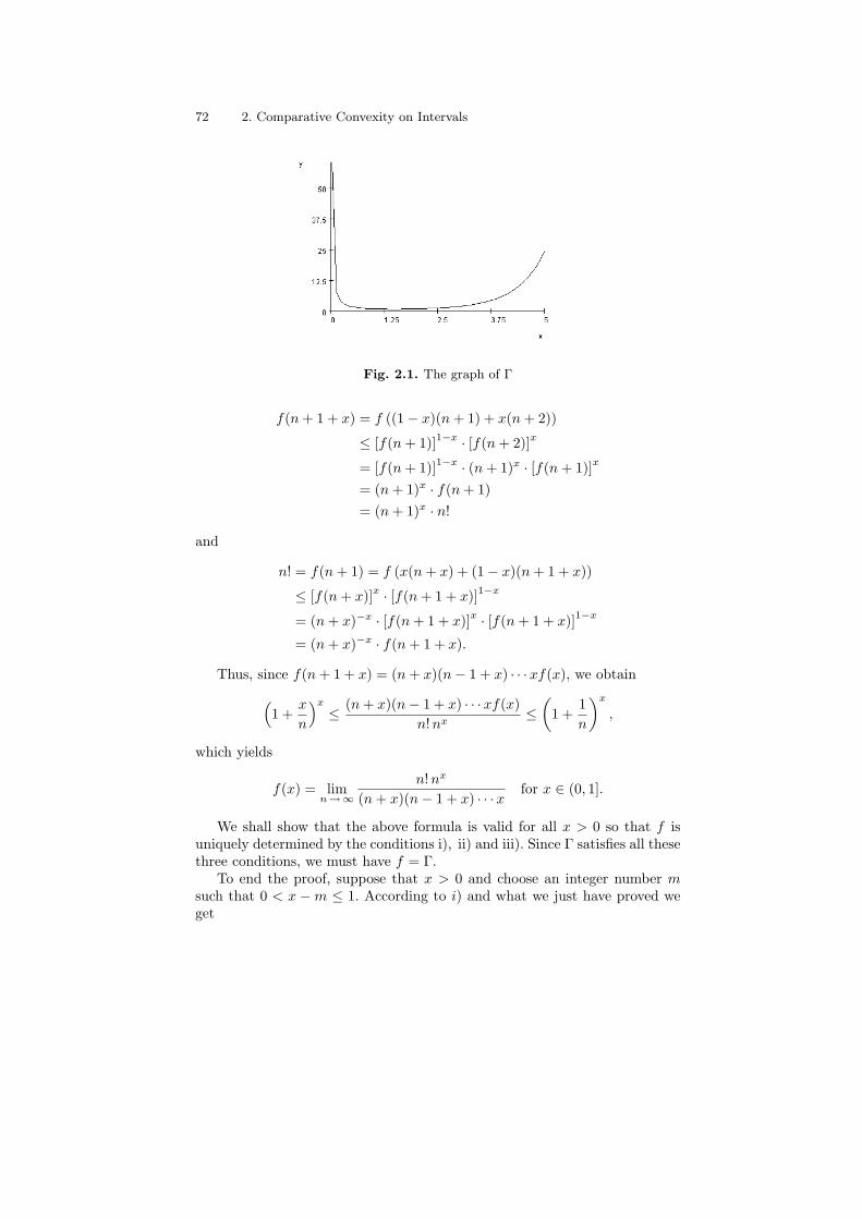
72 2. Comparative Convexity on Intervals
Fig. 2.1. The graph of Γ
f(n + 1 + x) = f ((1− x)(n + 1) + x(n + 2))
≤ [f(n + 1)]1−x · [f(n + 2)]x
= [f(n + 1)]1−x · (n + 1)x · [f(n + 1)]x
= (n + 1)x · f(n + 1)= (n + 1)x · n!
and
n! = f(n + 1) = f (x(n + x) + (1− x)(n + 1 + x))
≤ [f(n + x)]x · [f(n + 1 + x)]1−x
= (n + x)−x · [f(n + 1 + x)]x · [f(n + 1 + x)]1−x
= (n + x)−x · f(n + 1 + x).
Thus, since f(n + 1 + x) = (n + x)(n− 1 + x) · · ·xf(x), we obtain
(1 +
x
n
)x
≤ (n + x)(n− 1 + x) · · ·xf(x)n!nx
≤(
1 +1n
)x
,
which yields
f(x) = limn→∞
n!nx
(n + x)(n− 1 + x) · · ·x for x ∈ (0, 1].
We shall show that the above formula is valid for all x > 0 so that f isuniquely determined by the conditions i), ii) and iii). Since Γ satisfies all thesethree conditions, we must have f = Γ.
To end the proof, suppose that x > 0 and choose an integer number msuch that 0 < x −m ≤ 1. According to i) and what we just have proved weget

2.2. The Gamma and Beta Functions 73
f(x) = (x− 1) · · · (x−m) f(x−m)
= (x− 1) · · · (x−m) · limn→∞
n! nx−m
(n + x−m)(n− 1 + x−m) · · · (x−m)
= limn→∞
(n! nx
(n + x)(n− 1 + x) · · ·x ·
· (n + x)(n + x− 1) · · · (n + x− (m− 1))nm
)
= limn→∞
n!nx
(n + x)(n− 1 + x) · · ·x ·
· limn→∞
((1 +
x
n)(1 +
x− 1n
) · · · (1 +x−m + 1
n))
= limn→∞
n!nx
(n + x)(n− 1 + x) · · ·x . ¥
2.2.5. Corollary. Γ(x) = limn→∞
n!nx
(n + x)(n− 1 + x) · · ·x for all x > 0.
Before establishing a fundamental identity linking the gamma and sinefunctions, we need to express sin x as an infinite product:
2.2.6. Theorem (L. Euler). For all real numbers x,
sin x = x
∞∏
k = 1
(1− x2
k2π2
).
Proof. De Moivre’s formula shows that sin(2n + 1)θ is a polynomial of degree2n + 1 in sin θ (for each n ∈ N, arbitrarily fixed). This polynomial has roots± sin (kπ/(2n + 1)) for k = 0, ..., n. It follows that
sin(2n + 1)θ = (2n + 1) sin θ
n∏
k = 1
(1− sin2 θ
sin2 kπ2n+1
).
Suppose that x > 0 and fix arbitrarily two integers m and n such thatx < m < n. The last identity shows that
sin x
(2n + 1) sin x2n+1
=n∏
k = 1
(1− sin2 x
2n+1
sin2 kπ2n+1
).
Denote by ak the kth factor in this last product. Since 2θ/π < sin θ < θwhen 0 < θ < π/2, we find that
0 < 1− x2
4k2< ak < 1 for m < k ≤ n,
which yields

74 2. Comparative Convexity on Intervals
1 > am+1 · · · an >
n∏
k = 1
(1− x2
4k2
)> 1− x2
4
n∑
k = m+1
1k2
> 1− x2
4m.
Hencesin x
(2n + 1) sin x2n+1
lies between(
1− x2
4m
) n∏
k = 1
(1− sin2 x
2n+1
sin2 kπ2n+1
)and
n∏
k = 1
(1− sin2 x
2n+1
sin2 kπ2n+1
)
and so, letting n →∞, we deduce that sin x/x lies between
(1− x2
4m
) ∞∏
k = 1
(1− x2
k2π2
)and
∞∏
k = 1
(1− x2
k2π2
).
The proof ends by letting m →∞. ¥2.2.7. Theorem. For all real x with 0 < x < 1,
Γ(x) Γ(1− x) =π
sin πx.
Proof. In fact, by Corollary 2.2.5 and Theorem 2.2.6 above we infer that
Γ(x) Γ(1− x) = limn→∞
n! nx n!n1−x
(n + x) · · ·x (n + 1− x) · · · (1− x)
=1
x∞∏
k = 1
(1− x2/k2)=
π
sin πx. ¥
2.2.8. Corollary. Γ(1/2) =√
π.
A variant of the last corollary is the formula
1√2π
∫
Re−t2/2 dt = 1
which appears in many places in mathematics, statistics and natural sciences.Another beautiful consequence of Theorem 2.2.4 is the following:
2.2.9. Theorem (The Gauss-Legendre duplication formula).
Γ(x
2
)Γ
(x + 1
2
)=
√π
2x−1Γ(x) for all x > 0.
Proof. Notice that the function

2.2. The Gamma and Beta Functions 75
f(x) =2x−1
√π
Γ(x
2
)Γ
(x + 1
2
)x > 0,
verifies the conditions i)-iii) in Theorem 2.2.4 and thus equals Γ. ¥We will prove Stirling’s formula, which is an important tool in analytic
number theory. We shall need the following lemma:
2.2.10. Lemma. The sequence (an)n whose nth term is
an = log n!−(
n +12
)log n + n
converges.
Proof. We shall show that the sequence is decreasing and bounded below. Infact,
an − an+1 =(
n +12
)log
(1 +
1n
)− 1 ≥ 0
since by the Hermite-Hadamard inequality applied to the convex function 1/xon [n, n + 1] we have
log(
1 +1n
)=
∫ n+1
n
dx
x≥ 1
n + 1/2.
A similar argument (applied to the concave function log x on [u, v]) yields∫ v
u
log x dx ≤ (v − u) logu + v
2,
so that (taking into account the monotonicity of the log function) we get
∫ n
1
log x dx =∫ 1+1/2
1
log x dx +∫ 2+1/2
1+1/2
log x dx + · · ·+∫ n
n−1/2
log x dx
≤ 12
log32
+ log 2 + · · ·+ log(n− 1) +12
log n
<12
+ log n!− 12
log n.
Since ∫ n
1
log x dx = n log n− n + 1,
we conclude that
an = log n!−(
n +12
)log n + n >
12
. ¥
2.2.11. Theorem (Stirling’s formula). n! ∼ √2πnn+1/2 e−n.
76 2. Comparative Convexity on Intervals
Proof. Under the notation of the previous lemma, put
bn = ean =n!
nn+1/2 e−nfor n = 1, 2, ...
Then the sequence (bn)n converges to some b > 0. Thus
b2n
b2n=
22n+1/2 (n!)2
n1/2 (2n)!→ b2
b= b as n →∞.
For n = 1, 2, ... let cn =n!n1/2
(n + 12 ) · · · 3
2 · 12
. Then by Corollary 2.2.5, (cn)n
converges to Γ(1/2) =√
π as n →∞. Hence
b2n
b2n= cn(1 +
12n
)√
2 →√
2π as n →∞
which yields b =√
2π. Consequently,
bn =n!
nn+1/2 e−n→√
2π as n →∞. ¥
Closely related to the gamma function is the beta function B, which is thereal function of two variables defined by the formula
B(x, y) =∫ 1
0
tx−1(1− t)y−1 dt for x, y > 0.
2.2.12. Theorem. The beta function has the following properties:i) B(x, y) = B(y, x) and B(x + 1, y) =
x
x + yB(x, y);
ii) B(x, y) is a log-convex function of x for each fixed y;
iii) B(x, y) =Γ(x) Γ(y)Γ(x + y)
.
Proof. i) The first formula is clear. For the second,
B(x + 1, y) =∫ 1
0
tx(1− t)y−1 dt
=∫ 1
0
(1− t)x+y−1 (t/(1− t))xdt
=[−(1− t)x+y
x + y
(t
1− t
)x]t=1
t=0
+∫ 1
0
x
x + ytx−1(1− t)y−1 dt
=x
x + yB(x, y).
ii) Let a, b, y > 0 and let λ, µ ≥ 0 with λ + µ = 1. By the Rogers-Holderinequality,
2.2. The Gamma and Beta Functions 77
B(λa + µb, y) =∫ 1
0
(ta−1(1− t)y−1
)λ (tb−1(1− t)y−1
)µdt
≤(∫ 1
0
ta−1(1− t)y−1 dt
)λ (∫ 1
0
tb−1(1− t)y−1dt
)µ
= Bλ(a, y) ·Bµ(a, y).
iii) Let y > 0 be arbitrarily fixed and consider the function
ϕy(x) =Γ(x + y)B(x, y)
Γ(y), x > 0.
Then ϕy is a product of log-convex functions and so it is itself log-convex.Also,
ϕy(x + 1) =Γ(x + y + 1) B(x + 1, y)
Γ(y)
=[(x + y) Γ(x + y)] [x/(x + y)] B(x, y)
Γ(y)= xϕy(x)
for all x > 0 and
ϕy(1) =Γ(1 + y)B(1, y)
Γ(y)= y
∫ 1
0
(1− t)y−1 dt = 1.
Thus ϕy = Γ by Theorem 2.2.4, and the assertion iii) is now clear. ¥
Exercises
1. Prove that Γ(n + 12 ) = (2n)!
√π
n! 4n for n ∈ N.2. The integrals
In =∫ π/2
0
sinn t dt (for n ∈ N)
can be computed easily via the recurrence formula nIn = (n− 1) In−2
(where n ≥ 2). Integrate the inequalities sin2n+1 x ≤ sin2n x ≤ sin2n−1 xover [0, π/2] to infer Wallis’ formula,
π
2= lim
n→∞
[2 · 21 · 3 ·
4 · 43 · 5 · · ·
2n · 2n
(2n− 1) · (2n + 1)
].
Remark. An alternative proof of this formula follows from Corollary 2.2.5,by noticing that π/2 = (Γ(1/2))2 /2.
3. Establish the formula
B(x, y) = 2∫ π/2
0
sin2x−1 t · cos2y−1 t dt for x, y > 0,
and infer from it that∫ π/2
0
sin2n t dt =(2n)! π
22n+1(n!)2for n ∈ N.
78 2. Comparative Convexity on Intervals
4. Use Corollary 2.2.5 to prove Weierstrass’ formula,
Γ(x) =e−γx
x
∞∏n= 1
(1 +
x
n
)−1
ex/n,
where γ = limn→∞
(1 + 12 + · · · 1
n − log n) = 0. 57722... is Euler’s constant.
5. (The Raabe integral). Prove that
Γ(
1p
)Γ
(2p
)· · ·Γ
(p− 1
p
)=
(2π)p−1/2
p1/2for all p ∈ N?.
Then infer the integral formula∫ x+1
x
log Γ(t) dt = x (log x− 1) +12
log 2π for all x ≥ 0.
[Hint : Notice that∫ x+1
xlog Γ(t) dt − x (log x− 1) is constant. The case
when x = 0 can be settled by using Riemann sums. ]6. (L. Euler). Prove the formula
∫ ∞
0
tx−1
1 + tdt =
π
sin πxfor 0 < x < 1.
[Hint : Put t = u/(1− u) and apply Theorem 2.2.12 iii). ]7. (An alternative proof of the log-convexity of Γ). Prove the formula
d2
dx2log Γ(x) =
∞∑n = 0
1(x + n)2
for x > 0.
8. (E. Artin [11]). Let U be an open convex subset of Rn and let the functionϕ : U × (a, b) → [0,∞) satisfy:i) ϕ(x, t) is Borel measurable in t for each fixed x;ii) ϕ(x, t) is log-convex in x for each fixed t.Consider also a measure µ on the Borel subsets of (a, b) such that ϕ(x, ·)is µ-integrable for each x ∈ U. Prove that
Φ(x) =∫ b
a
ϕ(x, t) dµ(t)
is log-convex on U.[Hint : Apply the Rogers-Holder inequality, noticing that
ϕ((1− λ)x + λy, t) ≤ (ϕ(x, t))1−λ (ϕ(y, t))λ. ]
9. (An alternative approach of the Bohr-Mollerup theorem [109]). Let g be areal-valued concave function on (0,∞) such that g(x)/x → 0 as x →∞.

2.3. Generalities on Multiplicatively Convex Functions 79
i) Prove that the difference equation
f(x + 1)− f(x) = g(x)
has one and only one convex solution f : (0,∞) → R with f(1) = 0, andthis solution is given by the formula
f(x) = −g(x) + x · limn→∞
(g(n)−
n−1∑
k=1
g(x + k)− g(k)x
).
ii) (A Stirling type formula). Prove the existence of the limit
c = limx→∞
(f(x) + g(x)−
∫ x+1/2
1/2
g(t) dt
).
Remark. The Bohr-Mollerup theorem concerns the case where g = logand f = log Γ.
2.3 Generalities on Multiplicatively Convex Functions
The class of multiplicatively convex functions can be easily described as beingconstituted by those functions f (acting on subintervals of (0,∞)) such thatlog f(x) is a convex function of log x :
2.3.1. Lemma. Suppose that f : I → (0,∞) is a function defined on asubinterval of (0,∞). Then f is multiplicatively convex if and only if
∣∣∣∣∣∣
1 log x1 log f(x1)1 log x2 log f(x2)1 log x3 log f(x3)
∣∣∣∣∣∣≥ 0
for all x1 ≤ x2 ≤ x3 in I; equivalently, if and only if,
f(x1)log x3f(x2)log x1f(x3)log x2 ≥ f(x1)log x2f(x2)log x3f(x3)log x1
for all x1 ≤ x2 ≤ x3 in I.
This is nothing but the translation (via Lemma 2.1.1) of the result ofLemma 1.3.2.
In the same spirit, we can show that every multiplicatively convex functionf : I → (0,∞) has finite lateral derivatives at each interior point of I (and theset of all points where f is not differentiable is at most countable). As a conse-quence, every multiplicatively convex function is continuous in the interior ofits domain of definition. Under the presence of continuity, the multiplicativeconvexity can be restated in terms of geometric mean:
80 2. Comparative Convexity on Intervals
2.3.2. Theorem. Suppose that I is a subinterval of (0,∞). A continuousfunction f : I → [0,∞) is multiplicatively convex if and only if
x, y ∈ I implies f(√
xy) ≤√
f(x)f(y).
Proof. The necessity is clear. The sufficiency part follows from the connectionbetween the multiplicative convexity and the usual convexity (as noticed inLemma 2.1.1) and the fact that midpoint convexity is equivalent to convexityunder the presence of continuity. See Theorem 1.1.3. ¥
Theorem 2.3.2 reveals the essence of multiplicative convexity as being theconvexity according to the geometric mean; in fact, under the presence ofcontinuity, the multiplicatively convex functions are precisely those functionsf : I → [0,∞) for which
x1, ..., xn ∈ I implies f( n√
x1 · · ·xn) ≤ n√
f(x1) · · · f(xn).
In this respect, it is natural to call a function f : I → (0,∞) multiplicativelyconcave if 1/f is multiplicatively convex and multiplicatively affine if f is ofthe form Cxα for some C > 0 and some α ∈ R.
A refinement of the notion of multiplicative convexity is that of strictmultiplicative convexity, which in the context of continuity will mean
f( n√
x1 · · ·xn) < n√
f(x1) · · · f(xn)
unless x1 = ... = xn. Clearly, our remark concerning the connection betweenthe multiplicatively convex functions and the usual convex functions has a”strict” counterpart.
A large class of strictly multiplicatively convex functions is indicated bythe following result:
2.3.3. Proposition (G. H. Hardy, J. E. Littlewood and G. Polya [100], The-orem 177, page 125). Every polynomial P (x) with nonnegative coefficients is amultiplicatively convex function on [0,∞). More generally, every real analyticfunction f(x) =
∑∞n = 0 cnxn with nonnegative coefficients is a multiplicatively
convex function on [0, R), where R denotes the radius of convergence.Moreover, except for the case of functions Cxn (with C > 0 and n ∈ N),
the above examples exhibit strictly multiplicatively convex functions (whichare also increasing and strictly convex).
Examples of such real analytic functions are:
exp, sinh and cosh on (0,∞);
tan, sec, csc and1x− cot x on (0, π/2);
arcsin on (0, 1];
− log(1− x) and1 + x
1− xon (0, 1).

2.3. Generalities on Multiplicatively Convex Functions 81
See the table of series of I. S. Gradshteyn and I. M. Ryzhik [90].
Proof. By continuity, it suffices to prove only the first assertion. Suppose thatP (x) =
∑Nn = 0 cnxn. According to Theorem 2.3.2, we have to prove that
x, y > 0 implies (P (√
xy))2 ≤ P (x)P (y),
or, equivalently,
x, y > 0 implies (P (xy))2 ≤ P (x2)P (y2).
The later implication is an easy consequence of Cauchy-Buniakovski-Schwarz inequality. ¥
The following result collects a series of useful remarks for proving themultiplicative convexity of concrete functions:
2.3.4. Lemma. i) If a function is log-convex and increasing, then it is strictlymultiplicatively convex.
ii) If a function f is multiplicatively convex, then the function 1/f isstrictly concave (and vice versa).
iii) If a function f is multiplicatively convex, increasing and one-to-one,then its inverse is multiplicatively concave (and vice versa).
iv) If a function f is multiplicatively convex, so is xα [f(x)]β (for all α ∈ Rand all β > 0).
v) If f is continuous, and one of the functions f(x)x and f(e1/ log x) ismultiplicatively convex, then so is the other.
In many cases the inequalities based on multiplicative convexity are betterthan the direct application of the usual inequalities of convexity (or yieldcomplementary information). This includes the multiplicative analogue of theHardy-Littlewood-Polya inequality of majorization:
2.3.5. Proposition. Suppose that x1 ≥ x2 ≥ · · · ≥ xn and y1 ≥ y2 ≥ · · · ≥ yn
are two families of numbers in a subinterval I of (0,∞) such that
x1 ≥ y1
x1x2 ≥ y1y2
...
x1x2 · · ·xn−1 ≥ y1y2 · · · yn−1
x1x2 · · ·xn = y1y2 · · · yn.
Thenf(x1)f(x2) · · · f(xn) ≥ f(y1)f(y2) · · · f(yn)
for every multiplicatively convex function f : I → (0,∞).
A result due to H. Weyl [247] (see also [157]) gives us the basic example ofa pair of sequences satisfying the hypothesis of Proposition 2.3.5: Consider a
82 2. Comparative Convexity on Intervals
matrix A ∈Mn(C) having the eigenvalues λ1, ..., λn and the singular numberss1, ..., sn, and assume that they are rearranged such that |λ1| ≥ · · · ≥ |λn|,and s1 ≥ · · · ≥ sn. Then:
∣∣∣∣∣m∏
k = 1
λk
∣∣∣∣∣ ≤m∏
k = 1
sk for m = 1, ..., n− 1 and
∣∣∣∣∣n∏
k = 1
λk
∣∣∣∣∣ =n∏
k = 1
sk .
Recall that the singular numbers of a matrix A are precisely the eigenvaluesof its modulus, |A| = (A?A)1/2; the spectral mapping theorem assures thatsk = |λk| when A is Hermitian. The fact that all examples come this way wasnoticed by A. Horn; see [157] for details.
According to the discussion above the following result holds:
2.3.6. Proposition. Let A ∈Mn(C) be any matrix having the eigenvaluesλ1, ..., λn and the singular numbers s1, ..., sn, listed such that |λ1| ≥ · · · ≥ |λn|and s1 ≥ · · · ≥ sn. Then
n∏
k = 1
f(sk) ≥n∏
k = 1
f(|λk|)
for every multiplicatively convex function f which is continuous on [0,∞).
In general it is not true that |λk| ≤ sk for all k. A counter example is givenby the matrix (
0 14 0
)
whose eigenvalues are λ1 = 2 > λ2 = −2 and the singular numbers ares1 = 4 > s2 = 1.
Exercises
1. Suppose that P is a polynomial with nonnegative coefficients. Prove that
P (x1) · · ·P (xn) ≥ (P ( n√
x1 · · ·xn))n for every x1, ..., xn ≥ 0.
The particular case where P (x) = 1+x is known as Huygens’ inequality.Remark. The above inequality is complemented by a remark made by C.H. Kimberling [128] to Chebyshev’s inequality, namely,
(P (1))n−1P (x1 · · ·xn) ≥ P (x1) · · ·P (xn)
if all xk are either in [0, 1] or in [1,∞).2. (The multiplicative analogue of Popoviciu’s inequality). Suppose there
is given a multiplicatively convex function f : I → (0,∞). Infer fromTheorem 2.3.5 that
f(x) f(y) f(z) f3 ( 3√
xyz) ≥ f2 (√
xy) f2 (√
yz) f2(√
zx)
for all x, y, z ∈ I. Moreover, for the strictly multiplicatively convex func-tions the equality occurs only when x = y = z.

2.3. Generalities on Multiplicatively Convex Functions 83
3. Notice that the inverse sine function is strictly multiplicatively convex on(0, 1] and infer the following two inequalities in a triangle ∆ABC :
sinA
2sin
B
2sin
C
2<
(sin
(12
3√
ABC
) )3
<18
sin A sin B sinC <(sin 3
√ABC
)3
<3√
38
unless A = B = C.4. (P. Montel [173]). Let I ⊂ (0,∞) be an interval and suppose that f is
a continuous and positive function on I. Prove that f is multiplicativelyconvex if and only if
2f(x) ≤ kα f(kx) + k−α f(x/k)
for all α ∈ R, x ∈ I, and k > 0, such that kx and x/k both belong to I.5. (The multiplicative mean). According to Lemma 2.1.1, the multiplicative
analog of the arithmetic mean is
M∗(f) = exp
(1
log b− log a
∫ log b
log a
log f(et) dt
)
= exp
(1
log b− log a
∫ b
a
log f(t)dt
t
),
that is, the geometric mean of f with respect to the measure dt/t. Noticethat
M∗(1) = 1inf f ≤ f ≤ sup f ⇒ inf f ≤ M∗(f) ≤ sup f
M∗(fg) = M∗(f) M∗(g).
i) Let f : [a, b] → (0,∞) be a continuous function defined on a subintervalof (0,∞) and let ϕ : J → (0,∞) be a multiplicatively convex continuousfunction defined on an interval J which includes the image of f. Provethat
ϕ (M∗(f)) ≤ M∗(ϕ f),
which is the multiplicative analogue of Jensen’s inequality.ii) Suppose that 0 < a < b and let f : [a, b] → (0,∞) be a multi-plicatively convex continuous function. Prove the following analogue ofHermite-Hadamard inequality,
f(√
ab) ≤ M∗(f) ≤√
f(a)f(b);
the left hand side inequality is strict unless f is multiplicatively affine,while the right hand side inequality is strict unless f is multiplicatively

84 2. Comparative Convexity on Intervals
affine on each of the subintervals [a,√
ab] and [√
ab, b]. These inequalitiescan be improved following an idea similar to that of Remark 1.9.3:
f(a1/2b1/2) ≤(f(a3/4b1/4)f(a1/4b3/4)
)1/2
≤ M∗(f)
≤(f(a1/2b1/2)
)1/2
f(a)1/4f(b)1/4
≤ (f(a)f(b))1/2.
iii) Notice that M∗(f) = exp(
b−alog b−log a
)for f = exp | [a, b] (0 < a < b).
Then, infer from ii) the inequalities:
a3/4b1/4 + a1/4b3/4
2<
b− a
log b− log a<
12
(a + b
2+√
ab
)
exp(
b− a
log b− log a
)<
eb − ea
b− a.
6. Let f : I → (0,∞) be a function which is multiplicatively convex ormultiplicatively concave and let a > 0.i) Prove that
(n∏
k=1
f(ak/n)
)1/n
>
(n+1∏
k=1
f(ak/(n+1))
)1/(n+1)
> M∗(f)
for all n = 1, 2, 3, ... in each of the following two cases:I = [1, a] (with a > 1) and f is strictly increasing;I = [a, 1] (with 0 < a < 1) and f a strictly decreasing.
ii) Prove that the above inequalities will be reversed in each of the follow-ing two cases:
I = [1, a] (with a > 1) and f is strictly decreasing;I = [a, 1] (with 0 < a < 1) and f is strictly increasing.
iii) Illustrate the assertions i) and ii) in the case of the functions 1 + log xand exp x, for x ≥ 1, and sin (πx/2) and cos (πx/2) , for x ∈ (0, 1].
2.4 Multiplicative Convexity of Special Functions
We start this section by noticing that the indefinite integral of a multiplica-tively convex function has the same nature:
2.4.1. Proposition (P. Montel [173]). Let f : [0, a) → [0,∞) be a continuousfunction which is multiplicatively convex on (0, a). Then
F (x) =∫ x
0
f(t) dt
2.4. Multiplicative Convexity of Special Functions 85
is also continuous on [0, a) and multiplicatively convex on (0, a).
Proof. Due to the continuity of F it suffices to show that
(F (√
xy))2 ≤ F (x) F (y) for all x, y ∈ [0, a),
which is a consequence of the corresponding inequality at the level of integralsums,
[√xy
n
n−1∑
k = 0
f
(k
√xy
n
)]2
≤[
x
n
n−1∑
k = 0
f(k
x
n
)][y
n
n−1∑
k = 0
f(k
y
n
)],
that is, of the inequality[
n−1∑
k = 0
f
(k
√xy
n
)]2
≤[
n−1∑
k = 0
f(k
x
n
)] [n−1∑
k = 0
f(k
y
n
)].
To see that the later inequality holds, first notice that[
f
(k
√xy
n
)]2
≤[
f(k
x
n
)] [f
(k
y
n
)]
and then apply the Cauchy-Buniakovski-Schwarz inequality. ¥According to Proposition 2.4.1, the logarithmic integral ,
Li(x) =∫ x
2
dt
log t, x ≥ 2,
is multiplicatively convex. This function is important in number theory. Forexample, if π(x) counts the number of primes p such that 2 ≤ p ≤ x, thenan equivalent formulation of the Riemann hypothesis is the existence of afunction C : (0,∞) → (0,∞) such that
|π(x)− Li(x)| ≤ C(ε)x1/2+ε for all x ≥ 2 and all ε > 0.
Since the function tan is continuous on [0, π/2) and strictly multiplicativelyconvex on (0, π/2), a repeated application of Proposition 2.4.1 shows that theLobacevski’s function,
L(x) = −∫ x
0
log cos t dt
is strictly multiplicatively convex on (0, π/2).Starting with t/ (sin t) (which is strictly multiplicatively convex on (0, π/2])
and then switching to (sin t) /t, a similar argument leads us to the fact thatthe integral sine function,
Si (x) =∫ x
0
sin t
tdt ,
86 2. Comparative Convexity on Intervals
is strictly multiplicatively concave on (0, π/2].Another striking fact is the following:
2.4.2. Proposition. Γ is a strictly multiplicatively convex function on [1,∞).
Proof. In fact, log Γ(1 + x) is strictly convex and increasing on (1,∞). More-over, an increasing strictly convex function of a strictly convex function isstrictly convex. Hence, F (x) = log Γ(1+ ex) is strictly convex on (0,∞) andthus
Γ(1 + x) = eF (log x)
is strictly multiplicatively convex on [1,∞). As Γ(1+x) = xΓ(x), we concludethat Γ itself is strictly multiplicatively convex on [1,∞). ¥
According to Proposition 2.4.2,
Γ3( 3√
xyz) < Γ(x) Γ(y) Γ(z) for all x, y, z ≥ 1
except the case where x = y = z.On the other hand, by the multiplicative version of Popoviciu’s inequality
(Exercise 2 in Section 2.3), we infer that
Γ(x) Γ(y) Γ(z) Γ3 ( 3√
xyz) ≥ Γ2 (√
xy) Γ2 (√
yz) Γ2(√
zx)
for all x, y, z ≥ 1; the equality occurs only for x = y = z.Another application of Proposition 2.4.2 is the fact that the function
Γ(2x + 1)/Γ(x + 1) is strictly multiplicatively convex on [1,∞). This canbe seen by using the Gauss-Legendre duplication formula given by Theorem2.2.9.
Exercises
1. (D. Gronau and J. Matkowski [91]). Prove the following converse to Propo-sition 2.4.2: If f : (0,∞) → (0,∞) verifies the functional equation
f(x + 1) = xf(x),
the normalization condition f(1) = 1, and f is multiplicatively convex onan interval (a,∞), for some a > 0, then f = Γ.
2. Let f : I → (0,∞) be a differentiable function defined on a subinterval Iof (0,∞) . Prove that the following assertions are equivalent:i) f is multiplicatively convex;ii) The function xf ′(x)/f(x) is nondecreasing;iii) f verifies the inequality
f(x)f(y)
≥(
x
y
)y·f ′(y) / f(y)
for all x, y ∈ I.
A similar statement works for the multiplicatively concave functions. Il-lustrate this fact by considering the restriction of sin(cos x) to (0, π/2).

2.5. An Estimate of the AM-GM Inequality 87
3. The psi function (also known as the digamma function) is defined by
Psi (x) =d
dxlog Γ(x) =
Γ′(x)Γ(x)
, x > 0
and it can be represented as
Psi (x) = −γ −∫ 1
0
tx−1 − 11− t
dt,
where γ is Euler’s constant. See [10], [90].i) Prove that the function Psi satisfies the functional equation
ψ(x + 1) = ψ(x) +1x
.
ii) Infer from Proposition 2.4.2 and the preceding exercise the inequality
Γ(x)Γ(y)
≥(
x
y
)y·Psi (y)
for every x, y ≥ 1.
4. Let f : I → (0,∞) be a twice differentiable function defined on a subin-terval I of (0,∞) . Prove that f is multiplicatively convex if and onlyif
x[f(x)f ′′(x)− f ′ 2(x)] + f(x)f ′(x) ≥ 0 for all x > 0.
Infer that the integral sine function is multiplicatively concave.
2.5 An Estimate of the AM-GM Inequality
Suppose that I is a subinterval of (0,∞) and that f : I → (0,∞) is a twicedifferentiable function. According to Lemma 2.1.1, the values of the parameterα ∈ R for which the function
ϕ(x) = f(x) · x(−α/2) log x
is multiplicatively convex on I are precisely those for which the function
Φ(x) = log ϕ(ex) = log f(ex)− α x2
2,
is convex on log(I). Since the convexity of Φ is equivalent to Φ′′ ≥ 0, we inferthat ϕ is multiplicatively convex if and only if α ≤ α(f), where
α(f) = infx∈ log(I)
d2
dx2log f(ex)
= infx∈ I
x2(f(x)f ′′(x)− (f ′(x))2) + xf(x) f ′(x)f(x)2
.

88 2. Comparative Convexity on Intervals
By considering also the upper bound
β(f) = supx∈ log(I)
d2
dx2log f(ex),
we arrive at the following result:
2.5.1. Lemma. Under the above hypotheses, we have
exp
α(f)
2n2
∑
1≤j < k≤n
(log xj − log xk)2
≤(
n∏
k = 1
f(xk)
)1/n
/ f
(n∏
k = 1
xk
)1/n
≤ exp
β(f)
2n2
∑
1≤j < k≤n
(log xj − log xk)2
for all x1, ..., xn ∈ I.
Particularly, for f(x) = ex, x ∈ [A,B] (where 0 < A ≤ B), we have α(f) =A and β(f) = B and we are led to the following improvement upon the AM -GM inequality:
2.5.2. Lemma. Suppose that 0 < A ≤ B and n ∈ N?. Then
A
2n2
∑
1≤j < k≤n
(log xj − log xk)2 ≤ 1n
n∑
k=1
xk −(
n∏
k = 1
xk
)1/n
≤ B
2n2
∑
1≤j < k≤n
(log xj − log xk)2
for all x1, . . . , xn ∈ [A,B].
Since1
2n2
∑
1≤j < k≤n
(log xj − log xk)2
represents the variance of the random variable whose distribution is(
log x1 log x2 ... log xn
1/n 1/n ... 1/n
),
Lemma 2.5.2 reveals the probabilistic character of the AM -GM inequality.Using the usual device to approximate the integrable functions by step func-tions, we can derive from Lemma 2.5.2 the following more general result:

2.6. (M, N)-Convex Functions 89
2.5.3. Theorem. Let (Ω, Σ, P ) be a probability field and let X be a randomvariable on this space, taking values in the interval [A,B], where 0 < A ≤ B.Then
A ≤ E(X)− eE(log X)
var (log X)≤ B.
Here E(Z) =∫
XZ(ω)dP (ω) represents the conditional expectation of the
random variable Z, and var (Z) = E ((Z − E(Z))2
)the variance of Z.
Exercises
1. (H. Kober; see [168], p. 81). Suppose that x1, . . . , xn are positive numbers,not all equal, and λ1, . . . , λn are positive numbers such that λ1+· · ·+λn =1. Prove that
A (x1, . . . , xn; λ1, . . . , λn)−G (x1, . . . , xn;λ1, . . . , λn)∑
i<j
(√xi −√xj
)2
lies between infi λi/ (n− 1) and supi λi.2. (P. H. Diananda; see [168], p. 83). Under the same hypothesis as in the
precedent exercise, prove that
A (x1, . . . , xn; λ1, . . . , λn)−G (x1, . . . , xn;λ1, . . . , λn)∑
i<j λiλj
(√xi −√xj
)2
lies between 1/ (1− infi λi) and 1/ infi λi.3. Suppose that x1, . . . , xn and λ1, . . . , λn are positive numbers such that
λ1 + · · · + λn = 1. Put An = A (x1, . . . , xn;λ1, . . . , λn) and Gn =G (x1, . . . , xn; λ1, . . . , λn) .i) Compute the integral
J(x, y) =∫ ∞
0
tdt
(1 + t)(x + yt)2.
ii) Infer that An/Gn = exp(∑n
k=1 λk(xk −An)2J(xk, An)).
2.6 (M, N)-Convex Functions
The four algebraic variants of convexity we considered in the preceding sec-tions can be embedded into a more general framework, by taking two regularmeans M and N (on the intervals I and J respectively) and calling a functionf : I → J to be (M, N)-midpoint convex if it satisfies
f(M(x, y)) ≤ N(f(x), f(y))

90 2. Comparative Convexity on Intervals
for every x, y ∈ I. As noticed in Introduction, if f is continuous, this yieldsthe (M, N)-convexity of f, that is,
f(M(x, y; 1− λ, λ)) ≤ N(f(x), f(y); 1− λ, λ)
for every x, y ∈ I and every λ ∈ [0, 1]. The sundry notions such as (M,N)-strict convexity, (M, N)-concavity etc. can be introduced in a natural way.
Many important results like the left hand side of Hermite-Hadamard in-equality and the Jensen inequality extend to this framework. See TheoremsA, B and C in the Introduction.
Other results, like Lemma 2.1.1, can be extended only in the context ofquasi-arithmetic means:
2.6.1. Lemma (J. Aczel [2]). If ϕ and ψ are two continuous and strictlymonotonic functions (on intervals I and J respectively) and ψ is increasing,then a function f : I → J is (M[ϕ], M[ψ])-convex if and only if ψ f ϕ−1 isconvex on ϕ(I) in the usual sense.
Proof. In fact, f is (M[ϕ],M[ψ])-convex if and only if
ψ(f(ϕ−1((1− λ)u + λv))
) ≤ (1− λ)ψ(f(ϕ−1(u)
)+ λψ
(f(ϕ−1(v)
)
for all u, v ∈ ϕ(I) and λ ∈ [0, 1]. ¥A nice illustration of Lemma 2.6.1 was recently given by D. Borwein, J.
Borwein, G. Fee and R. Girgensohn [36], who proved that the volume Vn(p)of the ellipsoid x ∈ Rn | ‖x‖Lp ≤ 1 is (H, G)-strictly concave as a functionof p :
2.6.2. Theorem. Given α > 1, the function Vα(p) = 2α Γ(1+1/p)α
Γ(1+α/p) verifies theinequality
V 1−λα (p)V λ
α (q) < Vα
(1
1−λp + λ
q
),
for all p, q > 0, p 6= q and all λ ∈ (0, 1).
Proof. According to Lemma 2.6.1 it suffices to prove that the function
Uα(x) = − log (Vα(1/x)/2α) = log Γ(1 + αx)− α log Γ(1 + x)
is strictly convex on (0,∞) for every α > 1. Using the psi function,
Psi (x) =d
dx(log Γ(x)) ,
we haveU′′α (x) = α2 d
dxPsi (1 + αx)− α
d
dxPsi (1 + x).
Then U′′α (x) > 0 on (0,∞) means (x/α)U
′′α (x) > 0 on (0,∞), and the latter
holds if the function x → x ddxPsi (1 + x) is strictly increasing. Or, according
to [10], [90],
2.6. (M, N)-Convex Functions 91
d
dxPsi (1 + x) =
∫ ∞
0
u eux
eu − 1du,
and an easy computation shows that
d
dx
(x
d
dxPsi (1 + x)
)=
∫ ∞
0
u [(u− 1) eu + 1] eux
(eu − 1)2du > 0. ¥
As noticed in [36], p. 634, the volume function Vn(p) is neither convex norconcave for n ≥ 3.
In the next chapter we shall encounter the class of Mp-convex functions(−∞ ≤ p ≤ ∞). A function f : I → R is said to be Mp-convex if
f((1− λ)x + λy) ≤ Mp(f(x), f(y); 1− λ, λ)
for all x, y ∈ I and all λ ∈ [0, 1] (that is, f is (A,Mp)-convex). In order toavoid trivial situations, the theory of Mp-convex functions is usually restrictedto nonnegative functions when p ∈ R, p 6= 1.
The case p = 1 corresponds to the usual convex functions, while for p =0 we retrieve the log-convex functions. The case where p = ∞ is that ofquasiconvex functions that is, of functions f : I → R such that
f((1− λ)x + λy) ≤ sup (f(x), f(y)for all x, y ∈ I and all λ ∈ [0, 1]. Clearly, a function f : I → R is quasiconvexif and only if its sublevel sets x | f(x) ≤ α are convex for all α ∈ R.
If p > 0 (or p < 0), a function f is Mp-convex if and only if fp is convex(or concave, respectively). According to Exercise 8 in Section 1.1,
Mp(x, y; 1− λ, λ) ≤ Mq(x, y; 1− λ, λ) for −∞ ≤ p ≤ q ≤ ∞,
which shows that every Mp-convex function is also Mq-convex for all q ≥ p.
Exercises
1. Suppose that I and J are nondegenerate intervals and p, q, r ∈ R, p < q.Prove that for every function f : I → J the following two implicationshold true:
If f is (Mq,Mr)-convex and increasing, then it is also (Mp,Mr)-convex;If f is (Mp,Mr)-convex and decreasing, then it is also (Mq,Mr)-convex.
Conclude that the function Vα(p) of Theorem 2.6.2 is also (A,G)-concaveand (H, A)-concave.
2. Suppose that M and N are two regular means (respectively on the inter-vals I and J) and the function N (·, 1) is concave. Prove that:i) for every two (M, N)-convex functions f, g : I → J, the function f + gis (M,N)-convex;ii) for every (M, N)-convex function f : I → J and α > 0, the functionαf is (M, N)-convex.
92 2. Comparative Convexity on Intervals
3. Suppose that f : I → R is a continuous function which is differentiableon int I. Prove that f is quasiconvex if and only if for each x, y ∈ int I,
f(y) ≤ f(x) implies f ′(x)(y − x) ≤ 0.
4. (K. Knopp and B. Jessen; see [100], p. 66). Suppose that ϕ and ψ aretwo continuous functions defined in an interval I such that ϕ is strictlymonotonic and ψ is increasing.i) Prove that
M[ϕ](x1, ..., xn;λ1, ..., λn) = M[ψ](x1, ..., xn; λ1, ..., λn)
for every finite family x1, ..., xn of elements of I and every finite familyλ1, ..., λn of nonnegative numbers with
∑nk=1 λk = 1 (n ∈ N?), if and only
if ψ ϕ−1 is affine, that is, ψ = αϕ+β for some constants α and β, α 6= 0.ii) Infer that any power mean Mp is a mean M[ϕ], where ϕ(x) =(xp − 1) /p, if p 6= 0, and ϕ(x) = log x, if p = 0.
5. (M. Nagumo, B. de Finetti and B. Jessen; see [100], p. 68). Let ϕ be acontinuous increasing function on (0,∞) such that the quasi-arithmeticmean M[ϕ] is positively homogeneous. Prove that M[ϕ] is one of the powermeans.[Hint. By Exercise 4 i), we can replace ϕ by ϕ− ϕ(1), so we may assumethat ϕ(1) = 0. The same argument yields two functions α and β such thatϕ(cx) = α(c)ϕ(x) + β(c) for all x > 0, c > 0. The condition ϕ(1) = 0shows that β = ϕ, so for reasons of symmetry,
ϕ(cx) = α(c)ϕ(x) + ϕ(c) = α(x)ϕ(c) + ϕ(x).
Letting fixed c 6= 1, we obtain that α is of the form α(x) = 1 + kϕ(x) forsome constant k. Then ϕ verifies the functional equation
ϕ(xy) = kϕ(x)ϕ(y) + ϕ(x) + ϕ(y)
for all x > 0, y > 0. When k = 0 we find that ϕ(x) = C log x for someconstant C, so M[ϕ] = M0. When k 6= 0 we notice that χ = kϕ+1 verifiesχ(xy) = χ(x)χ(y) for all x > 0, y > 0. This leads to ϕ(x) = (xp − 1) /k,for some p 6= 0, so M[ϕ] = Mp. ]
6. (Convexity with respect to Stolarsky’s means). One can prove that theexponential function is (L,L)-convex. See Exercise 5 iii), at the end ofSection 2.3. Prove that this function is also (I, I)-convex. What can besaid about the logarithmic function? Here L and I are respectively thelogarithmic mean and the identric mean.
7. (Few affine functions with respect to the logarithmic mean; see [159]).Prove that the only (L,L)-affine functions f : (0,∞) → (0,∞) are theconstant functions and the linear functions f(x) = cx, for c > 0. Inferthat the logarithmic mean is not a power mean.
2.7. Relative Convexity 93
2.7 Relative Convexity
The comparison of quasi-arithmetic means is related to convexity via thefollowing result:
2.7.1. Lemma. Suppose that ϕ,ψ : I → R are two strictly monotonic contin-uous functions. If ϕ is increasing, then
M[ψ] ≤ M[ϕ]
if and only if ϕ ψ−1 is convex.
Lemma 2.7.1 has important consequences. For example, it yields Clark-son’s inequalities (which in turn extend the parallelogram law). The followingapproach (in the spirit of Orlicz spaces) is due to J. Lamperti [138]:
2.7.2. Theorem. Suppose that Φ : [0,∞) → R, is an increasing and contin-uous function with Φ(0) = 0 and Φ(
√x) convex. Consider a σ-finite measure
space (X,Σ, µ) and denote by LΦ(X) the set of all equivalence classes of allµ-measurable real-valued functions f such that
IΦ(f) =∫
X
Φ(|f(x)|) dµ < ∞.
i) If f + g and f − g belong to LΦ(X), then
IΦ(f + g) + IΦ(f − g) ≥ 2IΦ(f) + 2IΦ(g). (2.1)
If Φ(√
x) is concave and f and g belong to LΦ(X), then the reverse inequalityis true. If the convexity or concavity of Φ(
√x) is strict, equality holds in (2.1)
if and only if fg = 0 almost everywhere.
2.7.3. Corollary (Clarkson’s inequalities [58]). If 2 ≤ p < ∞, and f and gbelong to Lp(µ), then
‖f + g‖pLp + ‖f − g‖p
Lp ≥ 2 ‖f‖pLp + 2 ‖g‖p
Lp .
If 0 < p ≤ 2, then the reverse inequality holds. In either case, if p 6= 2,equality occurs if and only if fg = 0 almost everywhere.
Clarkson’s inequalities imply easily the uniform convexity of the spacesLp(µ) for 1 < p < ∞. See Exercise 2. J. Lamperti applied Corollary 2.7.3 togive the general form of the linear isometries T : Lp(µ) → Lp(µ), for p > 0,p 6= 2.
Clarkson’s inequalities are improved on by Hanner’s inequalities. See Ex-ercise 7 in Section 3.6.
Proof of Theorem 2.7.2. It suffices to prove the following result: Suppose thatΦ : [0,∞) → R is a continuous increasing function with Φ(0) = 0 and Φ(
√t)
convex. Then
94 2. Comparative Convexity on Intervals
Φ (|z + w|) + Φ (|z − w|) ≥ 2Φ (|z|) + 2Φ (|w|) , (2.2)
for all z, w ∈ C, while if Φ(√
t) is concave the reverse inequality is true.Provided the convexity or concavity is strict, equality holds if and only if
zw = 0.In fact, since Φ(
√t) is convex, we infer from Lemma 2.7.1 and the paral-
lelogram law the inequality
Φ−1
Φ (|z + w|) + Φ (|z − w|)
2
≥
|z + w|2 + |z − w|2
2
1/2
(2.3)
=(|z|2 + |w|2
)1/2
.
On the other hand, the convexity of Φ(√
t) and the fact that Φ(0) = 0 yieldthat Φ(
√t)/t is nondecreasing, that is, t2/Φ(t) is nonincreasing (respectively
decreasing if the convexity is strict). See Theorem 1.3.1. Taking into accountthe result of Exercise 1, we infer
Φ−1 Φ (|z|) + Φ (|w|) ≤(|z|2 + |w|2
)1/2
(2.4)
and thus (2.2) follows from (2.3), (2.4) and the fact that Φ is increasing. WhenΦ(√
t) is strictly convex, we also obtain from Exercise 1 the fact that (2.4)(and thus (2.2)) is strict, unless z or w is zero. ¥
Lemma 2.7.1 leads us naturally to consider the following concept of relativeconvexity:
2.7.4. Definition. Suppose that f and g are two real-valued functions definedon the same set X and g is not a constant function. Then f is said to be convexrelative to g (abbreviated, g C f) if
∣∣∣∣∣∣
1 g(x) f(x)1 g(y) f(y)1 g(z) f(z)
∣∣∣∣∣∣≥ 0,
whenever x, y, z ∈ X with g(x) ≤ g(y) ≤ g(z).
When X is an interval and g is continuous and increasing, a small com-putation shows that the condition g C f is equivalent with the convexity off g−1 (on the interval J = g(I)).
2.7.5. Examples. Under appropriate assumptions on the domain and therange of the function f, the following statements hold true:
i) f is convex if and only if id C f ;ii) f is log-convex if and only if id C log f ;iii) f is (G,G)-convex if and only if log C log f ;iv) f is (G,A)-convex if and only if log Cf.
2.7. Relative Convexity 95
A more exotic illustration of the concept of relative convexity is the fol-lowing fact:
f C fα for all f : X → R+ and all α ≥ 1.
For example, sinC sin2 on [0, π], and |x|C x2 on R.
In the context of C1-differentiable functions, f is convex with respectto an increasing function g if f ′/g′ is nondecreasing; in the context ofC2-differentiable functions, f is convex with respect to g if (and only if)f ′′/f ′ ≥ g′′/g′ (provided these ratios exist).
It is important to notice that relative convexity is part of comparativeconvexity. For, we need the integral analogue of quasi-arithmetic mean,
M[ϕ]
(id[s,t];
1t− s
dx
)= ϕ−1
(1
t− s
∫ t
s
ϕ(x) dx
).
In fact, if g C f, then
f
(M[g]
(id[a,b];
1b− a
dx
))= f
(g−1
(1
b− a
∫ b
a
g(x) dx
))
≤ 1b− a
∫ b
a
f(x) dx = M1(f |[a, b])
for all a < b in the domain of f and g.From the above discussion we can infer the following remark due to
H. Alzer [8]: Suppose that f is a strictly increasing continuous function(acting on subintervals of (0,∞)) and 1/f−1 is convex. Then 1/x C f. AsM[1/x](id[a,b]; 1
b−a dx) coincides with the logarithmic mean L(a, b), it followsthat
f(L(a, b)) ≤ 1b− a
∫ b
a
f(x) dx = M1(f |[a, b]).
We end this section by extending the Hardy-Littlewood-Polya inequalityto the context of relative convexity. Our approach is based on two technicallemmas.
2.7.6. Lemma. If f, g : X → R are two functions such that g C f, then
g(x) = g(y) implies f(x) = f(y).
Proof. Since g is not constant, then there must be a z ∈ X such that g(x) =g(y) 6= g(z). We may occur one of the following two cases:
Case 1: g(x) = g(y) < g(z). This yields
0 ≤∣∣∣∣∣∣
1 g(x) f(x)1 g(x) f(y)1 g(z) f(z)
∣∣∣∣∣∣= (g(z)− g(x)) (f(x)− f(y))
96 2. Comparative Convexity on Intervals
and thus f(x) ≥ f(y). A similar argument gives us the reverse inequality,f(x) ≤ f(y).
Case 2: g(z) < g(x) = g(y). This case can be treated in a similar way. ¥2.7.7. Lemma (The generalization of Galvani’s Lemma). If g Cf and x, u, vare points of X such that g(x) /∈ g(u), g(v) and g(u) ≤ g(v), then
f(v)− f(x)g(v)− g(x)
≥ f(u)− f(x)g(u)− g(x)
.
Proof. In fact, the following three cases may occur:Case 1: g(x) < g(u) ≤ g(v). Then
0 ≤∣∣∣∣∣∣
1 g(x) f(x)1 g(u) f(u)1 g(v) f(v)
∣∣∣∣∣∣= (g(u)− g(x)) (f(v)− f(x))− (g(v)− g(x)) (f(u)− f(x))
and the conclusion of Lemma 2.7.7 is clear.Case 2: g(u) ≤ g(v) < g(x). This case can be treated in the same way.Case 3: g(u) < g(x) < g(v). According to the discussion above we have
f(u)− f(x)g(u)− g(x)
=f(x)− f(u)g(x)− g(u)
≤ f(v)− f(u)g(v)− g(u)
=f(u)− f(v)g(u)− g(v)
≤ f(x)− f(v)g(x)− g(v)
=f(v)− f(x)g(v)− g(x)
and the proof is now complete. ¥2.7.8. Theorem (The generalization of the Hardy-Littlewood-Polya inequal-ity). Let f, g : X → R be two functions such that g C f and consider pointsx1, . . . , xn, y1, . . . , yn ∈ X and weights p1, . . . , pn ∈ R such that :
i) g(x1) ≥ . . . ≥ g(xn) and g(y1) ≥ . . . ≥ g(yn);
ii)r∑
k = 1
pk g(xk) ≤r∑
k = 1
pk g(yk) for every r = 1, . . . , n;
iii)n∑
k = 1
pk g(xk) =n∑
k = 1
pkg(yk).
Thenn∑
k = 1
pk f(xk) ≤n∑
k = 1
pk f(yk).
Proof. By mathematical induction. The case when n = 1 is clear. Assumingthe conclusion of Theorem 2.7.8 valid for all families of length n − 1, let uspass to the families of length n. The case when g(xk) = g(yk) for some indexk can be settled easily by our hypothesis and Lemma 2.7.6. Therefore we mayrestrict ourselves to the case when g(xk) 6= g(yk) for all indices k. By Abel’ssummation formula,

2.7. Relative Convexity 97
n∑
k = 1
pk f(yk)−n∑
k = 1
pk f(xk) (2.5)
equals
f(yn)− f(xn)g(yn)− g(xn)
(n∑
i = 1
pi g(yi)−n∑
i = 1
pi g(xi)
)+
+n−1∑
k = 1
(f(yk)− f(xk)g(yk)− g(xk)
− f(yk+1)− f(xk+1)g(yk+1)− g(xk+1)
) (k∑
i = 1
pi g(yi)−k∑
i = 1
pi g(xi)
)
which, by iii), reduces to
n−1∑
k = 1
(f(yk)− f(xk)g(yk)− g(xk)
− f(yk+1)− f(xk+1)g(yk+1)− g(xk+1)
) (k∑
i = 1
pi g(yi)−k∑
i = 1
pi g(xi)
).
According to ii), the proof will be complete if we shall show that
f(yk+1)− f(xk+1)g(yk+1)− g(xk+1)
≤ f(yk)− f(xk)g(yk)− g(xk)
for all indices k.In fact, if g(xk) = g(xk+1) or g(yk) = g(yk+1) for some index k, this follows
from i) and Lemmas 2.7.6 and 2.7.7.When g(xk) > g(xk+1) and g(yk) > g(yk+1) the following two cases may
occur:Case 1: g(xk) 6= g(yk+1). By a repeated application of Lemma 2.7.7 we get
f(yk+1)− f(xk+1)g(yk+1)− g(xk+1)
=f(xk+1)− f(yk+1)g(xk+1)− g(yk+1)
≤ f(xk)− f(yk+1)g(xk)− g(yk+1)
=f(yk+1)− f(xk)g(yk+1)− g(xk)
≤ f(yk)− f(xk)g(yk)− g(xk)
.
Case 2: g(xk) = g(yk+1). In this case, g(xk+1) < g(xk) = g(yk+1) < g(yk),and Lemmas 2.7.6 and 2.7.7 leads us to
f(yk+1)− f(xk+1)g(yk+1)− g(xk+1)
=f(xk)− f(xk+1)g(xk)− g(xk+1)
=f(xk+1)− f(xk)g(xk+1)− g(xk)
≤ f(yk)− f(xk)g(yk)− g(xk)
.
Consequently, (2.5) is a sum of nonnegative terms, and the proof is com-plete. ¥
The classical Hardy-Littlewood-Polya inequality corresponds to the casewhere X is an interval, g is the identity, and pk = 1 for all k. In this case, thehypothesis i) can be replaced by the following one:

98 2. Comparative Convexity on Intervals
i′) g(x1) ≥ . . . ≥ g(xn).
See Theorem 1.5.4. When X is an interval, g is the identity, and p1, . . . , pn
are arbitrary weights, then the result of Theorem 2.7.8 is known as Fuchs’inequality [84]. Clearly, Fuchs’ inequality implies Corollary 1.4.3 above.
In a similar way, we can extend another important result in majorizationtheory, the Tomic-Weyl theorem. See Exercise 5.
Exercises
1. (R. Cooper; see [100], p. 84). Suppose that ϕ,ψ : I → (0,∞) are twostrictly monotonic continuous functions which are onto. If ϕ and ψ varyin the same direction and ϕ/ψ is nonincreasing, then
ψ−1
(n∑
k=1
ψ(xk)
)≤ ϕ−1
(n∑
k=1
ϕ(xk)
)
for every finite family x1, ..., xn of elements of I.[Hint : If h(x)/x is nonincreasing for x > 0, then h(
∑nk=1 xk) ≤∑n
k=1 h(xk) for every finite family x1, ..., xn of points of (0,∞). See Exer-cise 8, Section 1.3. ]
2. Infer from Clarkson’s inequalities the uniform convexity of the spacesLp(µ), for 1 < p < ∞, that is, if x and y are in the unit ball of Lp(µ),then
inf
1−∥∥∥∥
x + y
2
∥∥∥∥ | ‖x− y‖ ≥ ε
> 0 when ε ∈ (0, 2].
3. Suppose that F, g : I → J are two continuous functions and g is strictlymonotonic. Prove that g C F if and only if for every α ≥ 0 and every[a, b] ⊂ I the function F − αg attains its maximum either at a or at b.Remark. This result can be used to prove sharpened versions of the max-imum principle for elliptic partial differential operators. See [244].
4. Suppose that f : [0, π/2] → R is a function such that
(f (y)− f (z)) cos x + (f (z)− f (x)) cos y + (f (x)− f (y)) cos z ≥ 0
for all x ≥ y ≥ z in [0, π/2]. Prove that
f(π
7
)− f
(2π
7
)+ f
(3π
7
)≤ f (0)− f
(π
3
)+ f
(π
2
).
5. (The extension of Tomic-Weyl theorem). Suppose that f, g : X → R aretwo synchronous functions with gCf . Consider points x1, . . . , xn, y1, . . . , yn
in X and real weights p1, . . . , pn such that:i) g(x1) ≥ . . . ≥ g(xn) and g(y1) ≥ . . . ≥ g(yn);ii)
∑mk = 1 pk g(xk) ≤ ∑m
k = 1 pk g(yk) for all m = 1, . . . , n.Prove that
n∑
k = 1
pk f(xk) ≤n∑
k = 1
pk f(yk).

2.8. Comments 99
2.8 Comments
The idea to transform by a change of variable a nonconvex function into aconvex one has a long history. As far as we know, the class of all multiplica-tively convex functions was first considered by P. Montel [173] in a beautifulpaper discussing the possible analogues of convex functions in n variables. Hementions in this respect the following two results:Hadamard’s Three Circles Theorem. Let f be an analytical function inthe annulus a < |z| < b. Then log M(r) is a convex function of log r, where
M(r) = sup|z|= r
|f(z)|,
G. H. Hardy’s Mean Value Theorem. Let f be an analytical functionin the annulus a < |z| < b and let p ∈ [1,∞). Then log Mp(r) is a convexfunction of log r, where
Mp(r) =(
12π
∫ 2π
0
|f(reiθ)|p dθ
)1/p
.
As limp→∞
Mp(r) = M(r), Hardy’s aforementioned result implies Hadamard’s.
It is well known that Hadamard’s result is instrumental in deriving the Riesz-Thorin interpolation theorem (see [100]).
The presentation of the class of multiplicatively convex functions (as wasdone in Sections 2.3 and 2.4) follows C. P. Niculescu [179]. The multiplicativemean (see [181] and Exercises 5 and 6 at the end of Section 2.3) providesthe right analogue of the arithmetic mean in a fully multiplicative theory ofconvexity.
The theory of Euler’s functions gamma and beta follows the same steps asin E. Artin [11] and R. Webster [245].
The quantum analogue of the gamma function, the q-gamma function Γq
of F. H. Jackson, is defined by
Γq(x) =(q; q)∞(qx; q)∞
(1− q)1−x for x > 0 (0 < q < 1)
where (a; q)∞ =∏∞
k=0
(1− aqk
). For it, the Bohr-Mollerup theorem has the
following form: Γq is the only solution of the functional equation
Γq(x + 1) =1− qx
1− qΓq(x),
which is log-convex and satisfies Γq(1) = 1. See [10]. D. Gronau and J.Matkowski [92] give an argument that Γq is multiplicatively convex at leaston (2,∞).
The well known inequalities in a triangle ∆ABC, such as
100 2. Comparative Convexity on Intervals
sin A + sin B + sin C ≤ 3√
3/2 and sinA sin B sin C ≤ 3√
3/8,
can be traced back to an old paper by G. Berkhan [22], from 1907.R. A. Satnoianu [224] noticed that the functions which are convex, multi-
plicatively convex and increasing are the source of Erdos-Mordell type inequal-ities in a triangle. Examples of such functions are numerous. See Proposition2.3.3.
The estimate given in Theorem 2.5.3 for the AM − GM inequality wasnoticed in [179].
The general notion of mean was clarified by B. de Finetti [81].The idea to consider the general notion of (M, N)-convex function (associ-
ated to a pair of means) can be traced to G. Aumann [14]. Later on, J. Aczel[2] considered the case of pairs of quasi-arithmetic means. The (M, N)-convexfunctions for M = N have been considered, for example, by J. Aczel [3], J.Matkowski [159], J. Matkowski and J. Ratz [160], [161]. The canonical exten-sion of a mean as well as Theorems A, B and C in the Introduction are dueto C. P. Niculescu [186].
The result of Exercise 5, Section 2.6, concerning the characterization ofthe power means among the quasi-arithmetic means, was recently extendedby J. Matkowski [159] to the context of strict and homogeneous means whichverify some nondegeneracy conditions.
The comparability Lemma 2.7.1 is due to B. Jessen. See [100], p. 75. Theconcept of relative convexity can be also traced to B. Jessen. See [100], The-orem 92, p. 75. Later, it was developed by G. T. Cargo [48], N. Elezovic andJ. Pecaric [72] and many others. The generalization of the classical inequal-ities of Hardy-Littlewood-Polya, Fuchs and Tomic-Weyl to the framework ofrelative convexity follows closely the paper [192] by C. P. Niculescu and F.Popovici.
Recently, M. Bessenyei and Z. Pales [27] have considered a more generalconcept of relative convexity, which goes back to a result of G. Polya; see[100], Theorem 123, p. 98. Given a pair (ω1, ω2) of continuous functions onan interval I, such that
∣∣∣∣ω1(x) ω1(y)ω2(x) ω2(y)
∣∣∣∣ 6= 0 for x < y, (2.6)
a function f : I → R is said to be (ω1, ω2)-convex if∣∣∣∣∣∣
f(x) f(y) f(z)ω1(x) ω1(y) ω1(z)ω2(x) ω2(y) ω2(z)
∣∣∣∣∣∣≥ 0
for all x < y < z in I. It is proved that the (ω1, ω2)-convexity implies thecontinuity of f at the interior points of I, as well as the integrability oncompact subintervals of I.
If I is an open interval, ω1 > 0 and the determinant in formula (2.6) is
positive, then f is (ω1, ω2)-convex if and only if the function fω1
(ω2ω1
)−1
2.8. Comments 101
is convex in the usual sense. Under these restrictions, M. Bessenyei and Z.Pales proved a Hermite-Hadamard type inequality. Notice that this case of(ω1, ω2)-convexity falls under the incidence of relative convexity.
Concerning the Clarkson type inequalities, there exists nowadays a lot ofinformation and several applications are pointed out. Here we just mentionthat even the general Edmunds-Triebel logarithmic spaces satisfy Clarkson’sinequalities See [193], where also some applications and relations to severalprevious results and references are presented.
A classical result due to P. Jordan and J. von Neumann asserts that theparallelogram law characterizes Hilbert spaces among Banach spaces. See M.M. Day [65], pp. 151-153. There are two important generalizations of theparallelogram law (both simple consequences of the inner-product structure).
The Leibniz-Lagrange identity. Suppose there is given a system of weightedpoints (x1,m1), ..., (xr, mr) in a inner-product space H, whose barycenter po-sition is
xG =r∑
k=1
mkxk/
r∑
k=1
mk.
Then for all points x ∈ H we have the equalities
r∑
k=1
mk ‖x− xk‖2 =
(r∑
k=1
mk
)‖x− xG‖2 +
r∑
k=1
mk ‖xG − xk‖2
=
(r∑
k=1
mk
)‖x− xG‖2 +
1∑rk=1 mk
·∑
i<j
mimj ‖xi − xj‖2 .
This identity is at the origin of many famous formulas concerning thedistances between some special points in a triangle. For example, in the casewhere x1, x2, x3 are the vertices of a triangle and m1,m2,m3 are proportionalto the length sides a, b, c, then xG is precisely the center I of the inscribedcircle. The above identity gives us (for x the center of the circumscribed circle)the celebrated formula of Euler ,
OI2 = R(R− 2r).
More information is vailable at www.neiu.edu/˜mathclub/˜Seminar notes.
E. Hlawka’s identity. We have
‖x‖2 + ‖y‖2 + ‖z‖2 + ‖x + y + z‖2 = ‖x + y‖2 + ‖y + z‖2 + ‖z + x‖2 ,
for all x, y, z in an inner-product space H.
This yields Hlawka’s inequality : In any inner-product space H, for allx, y, z ∈ H we have
‖x + y + z‖+ ‖x‖+ ‖y‖+ ‖z‖ − ‖x + y‖ − ‖y + z‖ − ‖z + x‖ ≥ 0.

102 2. Comparative Convexity on Intervals
In fact, based on Hlawka’s identity, the left hand side equals
(‖x‖+ ‖y‖ − ‖x + y‖)(
1− ‖x‖+ ‖y‖+ ‖x + y‖‖x‖+ ‖y‖+ ‖z‖+ ‖x + y + z‖
)
+(‖y‖+ ‖z‖ − ‖y + z‖)(
1− ‖y‖+ ‖z‖+ ‖y + z‖‖x‖+ ‖y‖+ ‖z‖+ ‖x + y + z‖
)
+(‖z‖+ ‖x‖ − ‖z + x‖)(
1− ‖z‖+ ‖x‖+ ‖z + x‖‖x‖+ ‖y‖+ ‖z‖+ ‖x + y + z‖
)
which is a combination of nonnegative terms.Hlawka’s inequality is not characteristic to Euclidean spaces! In fact, it was
extended by J. Lindenstrauss and A. PeÃlczynski [148] to all Banach spaces Ewhose finite dimensional subspaces can be embedded (linearly and isomet-rically) in suitable spaces Lp([0, 1]), with 1 ≤ p ≤ 2. On the other hand,Hlawka’s inequality doesn’t work for all Banach spaces. A counterexample isprovided by C2, endowed with the sup norm, and the vectors x = (1,−1),y = (i, i), z = (−i, 1).
A large generalization of Hlawka’s inequality, based on ergodic theory, wasgiven by M. Radulescu and S. Radulescu [213].
3
Convex Functions on a Normed Linear Space
Convex functions (and their relatives) provide basic techniques in a series ofdomains like optimization theory, partial differential equations and geometricinequalities related to isoperimetric problems. They are presented here in thecontext of real normed linear spaces (most of the time the Euclidean spaceRn).
3.1 Convex Sets
The natural domain for a convex function is a convex set. That’s why weshall start by recalling some basic facts on convex sets, which provide usefulfor understanding the general concept of convexity. All ambient linear spaceswill be supposed to be real.
A subset C of a linear space E is said to be convex if it contains the linesegment
[x, y] = (1− λ)x + λy |λ ∈ [0, 1]connecting any of its points x and y.
Fig. 3.1 below shows examples of convex and nonconvex sets. Besides these,convex sets in R2 include line segments, half-spaces, open or closed triangles,open discs (plus any part of the boundary) etc.
Many other examples can be obtained by considering the operation withsets:
λA + µB = λx + µy |x ∈ A, y ∈ B ,
for A,B ⊂ E and λ, µ ∈ R. See Fig. 3.2. One can prove easily that λA + µBis convex provided that A and B are convex and λ, µ ≥ 0.
A subset M of E is said to be affine if it contains the whole line throughany two of its points. Algebraically, this means
x, y ∈ M and λ ∈ R implies (1− λ)x + λy ∈ M.

104 3. Convex Functions on a Normed Linear Space
Fig. 3.1. Convex and nonconvex planar sets.
Fig. 3.2. Algebraic sum of sets.
Clearly, any affine subset is also convex (but the converse is not true). It isimportant to notice that any affine subset A is just the translate of a (unique)linear subspace L (and all translates of a linear space represent affine sets).In fact, for every a ∈ A, the translate
L = A− a
is a linear space and it is clear that A = L+a. For the uniqueness part, noticethat if L and M are linear subspaces of E and a, b ∈ E such that
L + a = M + b,
then necessarily L = M and a−b ∈ L. This remark allows us to introduce theconcept of dimension for an affine set (as the dimension of the linear subspaceof which it is a translate).
Given a finite family x1, . . . , xn of points in E, an affine combination ofthem is any point of the form
x =n∑
k=1
λkxk
for some λ1, . . . , λn ∈ R, with∑n
k=1 λk = 1. If, in addition, λ1, . . . , λn ≥ 0, xis called a convex combination (of x1, . . . , xn).

3.1. Convex Sets 105
3.1.1. Lemma. A subset C of E is convex (respectively affine) if and only ifit contains every convex (respectively affine) combination of points of C.
Proof. The sufficiency part is clear, while the necessity part can be proved bymathematical induction. See the remark before Lemma 1.1.2. ¥
Given a subset A of E, the intersection co (A) of all convex subsets con-taining A is convex and thus it is the smallest set of this nature containing A.We call it the convex hull of A. By using Lemma 3.1.1, one can verify easilythat co (A) consists of all convex combination of elements of A. The affinevariant of this construction yields the affine hull of A, denoted aff (A). As aconsequence we can introduce the concept of dimension for convex sets to bethe dimension of their affine hulls.
3.1.2. Theorem (Caratheodory’s theorem). Suppose that A is a subset of alinear space E and its convex hull co (A) has dimension m. Then each pointx of co (A) is the convex combination of at most m + 1 points of A.
Proof. Suppose that x =∑n
k=0 λkxk, where xk ∈ A, λk > 0 and∑n
k=0 λk = 1.If n > m, then the set B = x0, . . . , xn verifies
dim (aff (B)) ≤ dim (aff (A)) = m ≤ n− 1
and thus x1 − x0, . . . , xn − x0 is a linearly dependent set. This gives us aset of real numbers µ1, . . . , µn, not all 0, such that
∑nk=0 µk (xk − x0) = 0 and∑n
k=0 µk = 0. Choose a t > 0 for which υk = λk − tµk ≥ 0 for k = 0, . . . , nand υk = 0 for some index k. This allows us to reduce the number of termsin the representation of x :
x =n∑
k=0
λkxk =n∑
k=0
(υk + tµk) xk =∑
k 6=j
υkxk,
while∑
k 6=j υk =∑n
k=1 υk =∑n
k=1 (λk − tµk) =∑n
k=0 λk = 1. ¥The sets of the form C =co (x0, . . . , xn) are usually called polytopes. If
x1 − x0, . . . , xn − x0 are linearly independent, then C is called an n-simplex(with vertices x0, . . . , xn); in this case, dimC = n. Any point x in an n-simplexC has a unique representation x =
∑nk=0 λkxk, as a convex combination. In
this case, the numbers λ0, . . . , λn are called the barycentric coordinates of x.An important class of convex sets are the convex cones. A convex cone in
E is a subset C with the following two properties:
C + C ⊂ C
λC ⊂ C for all λ ≥ 0.
Interesting examples are:
Rn+ = (x1, . . . , xn) ∈ Rn |x1, . . . , xn ≥ 0 , the nonnegative orthant;Rn
++ = (x1, . . . , xn) ∈ Rn |x1, . . . , xn > 0 ;
106 3. Convex Functions on a Normed Linear Space
Rn≥ = (x1, . . . , xn) ∈ Rn |x1 ≥ · · · ≥ xn ;
Sym +(n,R), the set of positive matrices A of Mn(R), that is, of those Asuch that
〈Ax, x〉 ≥ 0 for all x ∈ Rn;
Sym ++(n,R), the set of strictly positive matrices of Mn(R), that is, of allA ∈Mn(R) such that
〈Ax, x〉 > 0 for all x ∈ Rn, x 6= 0.
They are important because of the orderings they induce:
x ≤ y if and only if y − x ∈ C.
So far we have not used any topology, only the linear properties of thespace E have played a role.
Suppose now that E is a linear normed space. The following two resultsrelate convexity and topology:
3.1.3. Lemma. If U is a convex set in a linear normed space, then its interiorintU and its closure U are convex too.
Proof. For example, if x, y ∈ intU, and λ ∈ (0, 1), then
λx + (1− λ)y + u = λ (x + u) + (1− λ) (y + u) ∈ intU
for all u in a suitable ball Bε(0). This shows that intU is a convex set. Nowlet x, y ∈ U. Then there exist sequences (xk)k and (yk)k in U, converging to xand y respectively. This yields λx+(1−λ)y = limk→∞ [λxk + (1− λ)yk] ∈ Ufor all λ ∈ [0, 1], that is, U is convex too. ¥
Notice that affine sets in Rn are closed because finite dimensional subspacesare always closed.
3.1.4. Lemma. If U is an open set in a linear normed space E, then itsconvex hull is open. If E is finite dimensional and K is a compact set, thenits convex hull is compact.
Proof. For the first assertion, let x =∑m
k=0 λkxk be a convex combination ofelements of the open set U. Then x+u =
∑mk=0 λk (xk + u) for all u ∈ E, and
since U is open it follows that xk +u ∈ U for all k, provided that ‖u‖ is smallenough. Consequently, x + u ∈ co (U) for u in a ball Bε(0).
We pass now to the second assertion. Clearly, we may assume that E = Rn.Then consider the map defined by
f(λ0, . . . , λn, x0, . . . , xn) =n∑
k=0
λkxk,
where λ0, . . . , λn ∈ [0, 1],∑n
k=0 λk = 1, and x0, . . . , xn ∈ K. Since f is con-tinuous and its domain of definition is a compact space, so is the range of f.

3.1. Convex Sets 107
According to Caratheodory’s theorem, the range of f is precisely co (K), andthis ends the proof. ¥
While working with a convex subset A of Rn, the natural space containingit is often aff (A) , not Rn, which may be far too large. For example, if dim A =k < n, then A has empty interior. We can talk more meaningfully about thetopological notions of interior and boundary by using the notions of relativeinterior and relative boundary. If A is a convex subset of Rn, the relativeinterior of A, denoted ri (A) , is the interior of A relative to aff (A) . That is,a ∈ ri (A) if and only if there is an ε > 0 such that Bε(a)∩ aff (A) ⊂ A. Wedefine the relative boundary of A, denoted rbd (A) , as rbd (A) = A \ ri (A) .These notions are important in optimization theory. See J. M. Borwein andA. S. Lewis [39].
Exercises
1. Let S = x0, . . . , xm be a finite subset of Rn. Prove that
ri (co S) =
m∑
k=0
λkxk |λk ∈ (0, 1) ,
m∑
k=0
λk = 1
.
2. Suppose that A and B are convex subsets of Rn, with A ⊂ B and aff (A) =aff (B) . Prove that ri (A) ⊂ ri (B) .
3. Prove that the relative interior of any nonempty convex subset A of Rn
is dense in A (and thus it is nonempty).4. (Accessibility lemma). Suppose that A is a convex subset of Rn, a ∈ ri (A)
and b ∈ A. Prove that
[a, b) = (1− λ)a + λb |λ ∈ [0, 1) ⊂ ri (A) .
Infer that ri (A) and int (A) are also convex.5. It is well known that all norms on Rn give rise to the same topology. Prove
that all (nonempty) open convex subsets of Rn are homeomorphic.[Hint : If B is the open unit ball of the Euclidean space Rn, then themapping x → x/(1 − ‖x‖2) provides a homeomorphism between B andRn. ]
6. A subset S = x0, . . . , xm of Rn is said to be affinely independent if thefamily x1 − x0, . . . , xm − x0 is linearly independent.Prove that this means
m∑
k=0
λkxk = 0 andm∑
k=0
λk = 0 imply λk = 0 for all k ∈ 0, . . . ,m .
Infer that an affinely independent set in Rn can have at most n+1 points.

108 3. Convex Functions on a Normed Linear Space
7. (Helly’s theorem; see [216] for applications). Let (Ci)i∈I be a finite col-lection of convex sets in Rn, where |I| ≥ n + 1. If every subcollection ofat most n + 1 sets has a nonempty intersection, then the entire collectionhas a nonempty intersection.[Hint : The statement is clear for |I| = n+1. Then assume that |I| > n+1and that the statement has already been proved for collections of |I| − 1sets. Choose for each i an element xi ∈ ∩j 6=iCj . Since |I| > n + 1 thesepoints are affinely dependent, which yields real scalars λi (i ∈ I), not allnull, such that ∑
i∈I
λixi = 0 and∑
i∈I
λi = 0.
Put λ =∑
i∈I λ+i =
∑i∈I λ−i . Then λ > 0 and
x =∑
i∈I
(λ+
i /λ)xi =
∑
i∈I
(λ−i /λ
)xi
belongs to ∩i∈ICi. Consider the two cases, λj ≥ 0 and λj < 0. ]Remark. Helly’s theorem is equivalent with Caratheodory’s theorem.
3.2 The Orthogonal Projection
In any normed linear space E we can speak on the distance of a point u ∈ Eto a subset A ⊂ E. This is done by the formula
d(u,A) = inf ‖u− a‖ | a ∈ Aand represents a numerical indicator of how well can u be approximated by theelements of A. When E = R3 and A is the x0y plane, the Pythagorean theoremshows that d(u,A) is precisely the distance between u and its orthogonalprojection on that plane.
This remark has a notable generalization which will be presented in whatfollows.
3.2.1. Theorem. Let C be a nonempty closed convex subset of a Hilbert spaceH (particularly, of the Euclidean space Rn). Then for each x ∈ H there is andis unique a point PC (x) of C such that
‖x− PC (x)‖ = d(x,C),
that is, there exists a unique nearest point of C to x.We call PC (x) the orthogonal projection of x onto C.
Proof. The existence of PC (x) follows from the definition of the distance ofa point to a set and the special geometry of the ambient space. In fact, anysequence (yn)n in C such that ‖x− yn‖ → α = d(x,C) is a Cauchy sequence.This is a consequence of the following identity,

3.2. The Orthogonal Projection 109
‖ym − yn‖2 + 4∥∥∥∥x− ym + yn
2
∥∥∥∥2
= 2(‖x− ym‖2 + ‖x− yn‖2
),
(motivated by the parallelogram law) and the definition of α as an infimum.They yield
∥∥x− ym+yn
2
∥∥ ≥ α, so that lim supm,n→∞ ‖ym − yn‖2 = 0.As H is complete, there must exist a point y ∈ C at which (yn)n converges.
Then necessarily d(x, y) = d(x,C). The uniqueness of y with this propertyfollows again from the parallelogram law. If y′ is another point of C such thatd(x, y′) = d(x,C) then
‖y − y′‖2 + 4∥∥∥∥x− y + y′
2
∥∥∥∥2
= 2(‖x− y‖2 + ‖x− y′‖2
)
which gives us ‖y − y′‖2 ≤ 0, a contradiction since it was assumed that thepoints y and y′ are distinct. ¥
The map PC : x→PC (x) , from H into itself, is called the orthogonalprojection associated to C. Clearly,
PC (x) ∈ C for every x ∈ Rn
andPC (x) = x if and only if x ∈ C.
Particularly,P 2
C = PC .
PC is also monotone, that is,
〈PC (x)− PC(y), x− y〉 ≥ 0 for every x, y ∈ H. (3.1)
This follows by adding the inequalities ‖x− PC (x)‖2 ≤ ‖x− PC(y)‖2 and‖y − PC (y)‖2 ≤ ‖y − PC(x)‖2 , after replacing the norm by the inner product.
If C is a closed subspace of the Hilbert space H, then PC is a linear self-adjoint projection and x − PC(x) is orthogonal on each element of C. Thisfact is basic for the entire theory of orthogonal decompositions.
Extensions of Theorem 3.2.1 are indicated in Exercise 4 and Theorem C.1.1(Appendix C).
It is important to reformulate Theorem 3.2.1 in the framework of approx-imation theory. Suppose that C is a nonempty closed subset in a real linearnormed space E. We define the set of best approximation from x ∈ E to C asthe set PC(x) of all points in C closest to x, that is,
PC(x) = z ∈ C | d(x,C) = ‖x− z‖ 6= ∅.
We say that C is a Chebyshev set if PC(x) is a singleton for all x ∈ E, and aproximinal set if all the sets PC(x) are nonempty. Theorem 3.2.1 asserts thatall nonempty closed convex sets in a Hilbert space are Chebyshev sets. There

110 3. Convex Functions on a Normed Linear Space
is an analogue of this theorem valid for all spaces Lp(µ) (1 < p < ∞, p 6= 2),saying that all such sets are proximinal. See Exercise 8, Section 3.6.
Clearly, the Chebyshev sets are closed. The following result is a partialconverse to Theorem 3.2.1:
3.2.2. Theorem (L. N. H. Bunt). Every Chebyshev subset of Rn is convex.
See R. Webster [245], pp. 362-365, for a proof based on Brouwer’s fixedpoint theorem. Proofs based on the differentiability properties of the functiondC : x → d(x, C), are available in the paper of J.-B. Hiriart-Urruty [106],and in the monograph of L. Hormander [109], pp. 62-63. They are sketchedin Exercise 3, Section 3.8, and Exercise 3, Section 3.11.
V. Klee raised the question whether Theorem 3.2.2 is valid for all realHilbert spaces. The answer is known to be positive for all Chebyshev sets Csuch that the map d2
C is differentiable. See [106] for details (and an accounton Klee’s problem).
Exercises
1. Find an explicit formula for the orthogonal projection PC when C is aclosed ball Br(a) in Rn.
2. Let `∞(n,R) be the space Rn endowed with the sup norm, ||(x1, x2)|| =sup |x1| , |x2| , and let C be the set of all vectors (x1, x2) such thatx2 ≥ x1 ≥ 0. Prove that C is a nonconvex Chebyshev set.
3. Consider in Rn the nonconvex set C =(x1, x2) |x2
1 + x22 ≥ 1
. Prove
that all points of Rn except the origin admit a unique closest point in C.4. (Lions-Stampacchia theorem on a-projections). Let H be a real Hilbert
space and let a : H × H → R be a coercive continuous bilinear form.Coercivity is meant here as the existence of a positive constant c suchthat a(x, x) ≥ c ‖x‖2 for all x ∈ H. Prove that for each x ∈ H and eachnonempty closed convex subset C of H there exists a unique point v in C(called the a-projection of x onto C) such that
a(x− v, y − v) ≤ 0 for all y ∈ C.
Remark. This theorem has important applications in partial differentialequations and optimization theory. See, for example, [15], [70], [71].
3.3 Hyperplanes and Separation Theorems
The notion of a hyperplane represents a natural generalization of the notionof a line in R2 or a plane in R3. Hyperplanes prove useful to split the wholespace into two pieces (called half-spaces).
A hyperplane in a real linear space E is any set of constancy of a nonzerolinear functional. In other words, a hyperplane is a set of the form
3.3. Hyperplanes and Separation Theorems 111
H = x ∈ E |h(x) = α , (3.2)
where h : E → R is a suitable nonzero linear functional and α is a suitablescalar. In this case the sets
x ∈ E |h(x) ≤ α and x ∈ E |h(x) ≥ α
are called the half-spaces determined by H. We say that H separates twosets U and V if they lie in opposite half-spaces (and separates strictlyU and V if one set is contained in x ∈ E |h(x) < α and the other inx ∈ E |h(x) ≥ α).
When the functional h which appears in the representation formula (3.2)is continuous (that is, when h belongs to the dual space E′) we say thatthe corresponding hyperplane H is closed. In the context of Rn, all linearfunctionals are continuous and thus all hyperplanes are closed. In fact, anylinear functional h : Rn → R has the form h(x) = 〈x, z〉, for some z ∈ Rn
(uniquely determined by h). This follows directly from the linearity of h andthe representation of Rn with respect to the canonical basis:
h(x) = h
(n∑
k=1
xkek
)=
n∑
k=1
xkh(ek)
= 〈x, z〉,
where z =∑n
k=1 h(ek)ek is the gradient of h.Some authors define the hyperplane as the maximal proper affine subsets
H of E. Proper means here different from E. One can prove that the hyper-planes are precisely the translates of codimension-1 linear subspaces, and thisexplains the agreement of the two definitions.
The following results on the separation of convex sets by closed hyper-planes are part of a much more general theory that will be presented in Ap-pendix A:
3.3.1. Theorem (Separation theorem). Let U and V be two convex sets in anormed linear space E, with intU 6= ∅ and V ∩ intU = ∅. Then there exists aclosed hyperplane that separates U and V.
3.3.2. Theorem (Strong separation theorem). Let K and C be two disjointnonempty convex sets in a normed linear space E with K compact and Cclosed. Then there exists a closed hyperplane that separates strictly K and C.
The special case of this result when K is a singleton is known as the basicseparation theorem.
A proof of Theorems 3.3.1 and 3.3.2 in the finite dimensional case issketched in Exercises 1 and 2.
Next we introduce the notion of a supporting hyperplane to a convex setA (in a normed linear space E).

112 3. Convex Functions on a Normed Linear Space
3.3.3. Definition. We say that the hyperplane H supports A at a point a inA if a ∈ H and A is contained in one of the half-spaces determined by H.
Theorem 3.3.1 assures the existence of a supporting hyperplane to anyconvex set A at a boundary point, provided that A has nonempty interior.
When E = Rn, the existence of a supporting hyperplane of U at a bound-ary point a will mean the existence of a vector z ∈ Rn and of a real numberα such that
〈a, z〉 = α and 〈x, z〉 ≤ α for all x ∈ U.
A direct argument for the existence of a supporting hyperplane in the finitedimensional case is given in Exercise 3.
We end this section with a discussion on the geometry of convex sets infinite dimensional spaces.
3.3.4. Definition. Let U be a convex subset of a linear space E. A point z ofU is an extreme point of U if it is not an interior point of any linear segment inU, that is, if there do not exist distinct points x, y ∈ U and numbers λ ∈ (0, 1)such that
z = (1− λ)x + λy.
The extreme points of a triangle are its vertices. More generally, everypolytope A =co a0, . . . , am has finitely many extreme points, and they areamong the points a0, . . . , am.
All boundary points of a disc DR0) =(x, y) |x2 + y2 ≤ R2
are extreme
points; this is an expression of the rotundity of discs. The closed upper half-plane y ≥ 0 in R2 has no extreme point.
The extreme points are the landmarks of compact convex sets in Rn :
3.3.5. Theorem (H. Minkowski). Every convex and compact subset K of Rn
is the convex hull of its extreme points.
Proof. We use induction on the dimension m of K. If m = 0 or m = 1, thatis, when K is a point or a closed segment, the above statement is obvious.Assume the theorem is true for all compact convex sets of dimension at mostm ≤ n− 1. Consider now a compact convex set K whose dimension is m + 1and embed it into a linear subspace E of dimension m + 1.
If z is a boundary point of K, then we can choose a supporting hyperplaneH ⊂ E for K through z. The set K ∩ H is compact and convex and itsdimension is ≤ m. By the induction hypothesis, z is a convex combination ofextreme points of K∩H. Or, any extreme point e of K∩H is also an extremepoint of K. In fact, letting H = t ∈ E |ϕ(t) = α, we may assume that Kis included in the half-space ϕ(t) ≤ α. If e = (1 − λ)x + λy with x 6= y in Kand λ ∈ (0, 1), then necessarily ϕ(x) = ϕ(y) = α, that is, x and y should bein K ∩H, in contradiction with the choice of e.
If z is an interior point of K, then each line through z intersects K in asegment whose endpoints belong to the boundary of K. Consequently, z is a
3.3. Hyperplanes and Separation Theorems 113
convex combination of boundary points that in turn are convex combinationsof extreme points. This ends the proof. ¥
The result of Theorem 3.3.5 can be made more precise as follows: everypoint in a compact convex subset K of Rn is the convex combination of atmost n + 1 extreme points. See Theorem 3.1.2.
Exercises
1. Complete the following sketch of proof of Theorem 3.3.2 in the case whenE = Rn : First prove that the distance
d = inf‖x− y‖ |x ∈ K, y ∈ C
is attained for a pair x0 ∈ K, y0 ∈ C. Then notice that the hyperplanethrough x0, orthogonal to the linear segment [x0, y0], determined by x0
and y0, has the equation 〈y0 − x0, z − x0〉 = 0. Fix arbitrarily a pointx ∈ K. Then 〈y0−x0, z−x0〉 ≤ 0 for every point z ∈ [x0, x] (and thus forevery z ∈ K). Conclude that every hyperplane through any point insidethe segment [x0, y0], orthogonal to this segment, separates strictly K andC.
2. Infer the finite dimensional case of Theorem 3.3.1 from Theorem 3.3.2.[Hint : It suffices to assume that both sets U and V are closed. Thenchoose a point x0 ∈ intU and apply the preceding exercise to V and tothe compact set
Kn = x0 + (1− 1/n)(x− x0) |x ∈ U ∩Bn(0)
for n ∈ N?. This gives us a sequence of unit vectors un and numbersαn such that 〈un, x〉 ≤ αn for x ∈ Kn and 〈un, y〉 ≥ αn for y ∈ V . As(un)n and (αn)n are bounded, they admit converging subsequences, sayto u and respectively α. Conclude that H = z | 〈u, z〉 = α is the desiredseparation hyperplane. ]
3. (The support theorem). Assume that E = Rn and a is a point in therelative boundary of the convex subset A of E. Prove that there exists asupporting hyperplane H to A at a which differs from aff (A) .[Hint : We may assume that A is closed, by replacing A with A. Choose apoint x0 ∈ S1 (a) = x | ‖x− a‖ = 1 such that
d(x0, A) = sup d(x,A) |x ∈ S1 (a) ,
that is, x0 is the farthest point from A. Prove that a is the point of Aclosest to x0 and conclude that the hyperplane H = z | 〈x0−a, z−a〉 = 0supports U at a.
4. Prove that a closed convex set in Rn is the intersection of closed half-spaces which contain it.

114 3. Convex Functions on a Normed Linear Space
5. A set in Rn is a polyhedron if it is a finite intersection of closed half-spaces.Prove that:i) Every compact polyhedron is a polytope (the converse is also true);ii) Every polytope has finitely many extreme points;iii) Sym +(2,R) is a closed convex cone (with interior Sym ++(2,R)) butnot a polyhedron.
6. A theorem due to G. Birkhoff (see [245], pp. 246-247) asserts that everydoubly stochastic matrix is a convex combination of permutation matri-ces. As the set Ωn ⊂Mn(R) of all doubly stochastic matrices is compactand convex, and the extreme points of Ωn are the permutation matrices,Birkhoff’s result follows from Theorem 3.3.5.i) Verify this fact for n = 2.ii) Infer from it Rado’s characterization of majorization: x ≺ y in Rn ifand only if x belongs to the convex hull of the n! permutations of y.
7. Let C be a nonempty subset of Rn. The polar set of C, is the set
C = x ∈ Rn | 〈u, x〉 ≤ 1 for every u ∈ C .
i) Prove that C is a closed convex set containing 0 and C ⊂ D impliesD ⊂ C.ii) (The bipolar theorem). Infer from the basic separation theorem thatC = co (C ∪ 0).
3.4 Convex Functions in Higher Dimensions
The notion of a convex function can be extended in a straightforward mannerto the case of functions defined on an arbitrary convex set. In what follows Uwill be a convex set in a real linear space E.
3.4.1. Definition. A function f : U → R is said to be convex if
f((1− λ)x + λy) ≤ (1− λ)f(x) + λf(y) (3.3)
for all x, y ∈ U and all λ ∈ [0, 1].The other related notions such as concave function, affine function, strictly
convex function etc., can be introduced as in Section 1.1.
By mathematical induction we can extend the basic inequality (3.3) to thecase of arbitrary convex combinations. We shall refer to this as the discretecase of Jensen’s inequality.
Convexity in several variables case is equivalent with convexity on eachline segment included in the domain of definition:3.4.2. Proposition. A function f : U → R is convex if and only if for everytwo points x and y in U the function
ϕ : [0, 1] → R, ϕ(t) = f ((1− t)x + ty)
3.4. Convex Functions in Higher Dimensions 115
is convex.Notice that convexity of functions in the several variables case means more
than convexity in each variable separately; think at the case of the functionf(x, y) = xy, (x, y) ∈ R2, which is not convex, though convex in each variable.
Some simple examples of strictly convex functions on Rn are as follows:
f(x1, . . . , xn) =∑n
k=1 ϕ(xk), where ϕ is a strictly convex function on R.
f(x1, . . . , xn) =∑
i<j cij (xi − xj)2, where the coefficients cij are positive.
The distance function dU : Rn → R, dU (x) = d(x,U), associated to anonempty convex set U in Rn.
We shall next discuss several connections between convex functions andconvex sets.
By definition, the epigraph of a function f : U → R is the set
epi (f) = (x, y) |x ∈ U, y ∈ R and f(x) ≤ y .
It is easy to verify that f : U → R is convex if and only if epi (f) is convex inE ×R. This shows that the theory of convex functions can be subordinated tothe theory of convex sets.
A practical implication is the existence of supporting hyperplanes for con-vex functions. To make this more precise, we shall pass to the topological con-text where U is an open convex set in a linear normed space E and f : U → Ris a continuous convex function. In this case, epi (f) has nonempty interior inE ×R and every point (a, f(a)) is a boundary point for epi (f). According toTheorem 3.3.1, there is a closed hyperplane H in E×R that contains (a, f(a))and epi (f) is contained in one of the half-spaces determined by H. We callthis a supporting hyperplane to f at a.
The closed hyperplanes H are associated to nonzero continuous linearfunctionals on E × R and the dual space of E × R is constituted of all pairs(h, λ), where h is any continuous linear functional on E and λ is any realnumber. Consequently a supporting hyperplane to f at a is determined by apair (h, λ) and a real number α such that
h(a) + λf(a) = α
andh(x) + λy ≥ α for all y ≥ f(x) and all x ∈ U.
Notice that λ 6= 0, since otherwise h(x) ≥ h(a) for x in a ball Br(a), whichforces h = 0. A moment’s reflection shows that actually λ > 0 and thus weare led to the existence of a continuous linear functional h such that
f(x) ≥ f(a) + h(x− a) for every x ∈ U.
We call h a support of f at a.

116 3. Convex Functions on a Normed Linear Space
From this point we can continue as in the case of functions of one variable,by developing the concept of subdifferential. We shall come back to this matterin Section 3.7.
We pass now to another connection between convex functions and convexsets.
Given a function f : U → R and a scalar α, the sublevel set Lα of f atheight α is the set
Lα = x ∈ U | f(x) ≤ α .
3.4.3. Lemma. Each sublevel set of a convex function is a convex set.
The property of Lemma 3.4.3 characterizes the quasiconvex functions. SeeExercise 8.
Convex functions exhibit a series of nice properties related to maxima andminima, which made them important in theoretical and applied mathematics.
3.4.4. Theorem. Assume that U is a convex subset of a normed linear spaceE. Then any local minimum of a convex function f : U → R is also a globalminimum. Moreover, the set of global minimizers of f is convex.
If f is strictly convex in a neighborhood of a minimum point, then theminimum point is unique.
Proof. If a is a local minimum, then for each x ∈ U there is an ε > 0 suchthat
f(a) ≤ f (a + ε(x− a)) = f ((1− ε)a + εx) (3.4)≤ (1− ε)f(a) + εf(x).
This yields f(a) ≤ f(x), so a is a global minimum. If f is strictly convexin a neighborhood of a, then the last inequality in (3.4) is strict and theconclusion becomes f(x) > f(a) for all x ∈ U, x 6= a. The second assertion isa consequence of Lemma 3.4.3. ¥
The following result gives us a useful condition for the existence of a globalminimum:
3.4.5. Theorem (K. Weierstrass). Assume that U is an unbounded closedconvex set in Rn and f : U → R is a continuous convex function whosesublevel sets are bounded. Then f has a global minimum.
Proof. Notice that all sublevel sets Lα of f are bounded and closed (andthus compact in Rn). Then every sequence of elements in a sublevel set hasa converging subsequence and this yields immediately the existence of globalminimizers. ¥
The condition on boundedness of sublevel sets is equivalent with the fol-lowing growth condition:
lim inf‖x‖→∞
f(x)‖x‖ > 0. (3.5)
3.4. Convex Functions in Higher Dimensions 117
The sufficiency part is clear. For the necessity part, reason by reductio adabsurdum.
The functions which verify the condition (3.5) are said to be coercive.Clearly, coercivity implies
lim‖x‖→∞
f(x) = ∞.
Convex functions attain their maxima at the boundary:
3.4.6. Theorem (The maximum principle). If f is a convex function on aconvex subset U of a normed linear space E and attains a global maximum atan interior point of U, then f is constant.
Proof. Assume that f is not constant and attains a global maximum ata ∈ intU . Choose x ∈ U such that f(x) < f(a) and ε ∈ (0, 1) such thaty = a + ε(a− x) ∈ U. Then a = 1
1+εy + ε1+εx, which yields to a contradiction
since
f(a) ≤ 11 + ε
f(y) +ε
1 + εf(x)
<1
1 + εf(a) +
ε
1 + εf(a) = f(a). ¥
A generalization of the maximum principle is given in Corollary A.4.3 (Ap-pendix A). We end this section with an important consequence of Theorems3.3.5 and 3.4.7:
3.4.7. Theorem. If f is a continuous convex function on a compact convexsubset K of Rn, then f attains a global maximum at an extreme point.
Proof. Assume that f attains its global maximum at a ∈ K. By Theorem 3.3.5,a can be represented as a convex combination of extreme points, say a =∑n
k=1 λkek. Then f(a) ≤ ∑nk=1 λkf(ek) ≤ supk f(ek), which forces f(a) =
f(ek) for some k. ¥For functions defined on n-dimensional intervals [a1, b1] × . . . × [an, bn]
in Rn, Theorem 3.4.7 extends to the case of continuous functions which areconvex in each variable (when the others are kept fixed). This fact can beproved by one-variable means (taking into account Theorem 1.1.3). A sampleis offered by Exercise 3.
In the infinite dimensional setting, it is difficult to state fairly general re-sults on maximum-attaining. Besides, the deep results of Banach space theoryappears to be crucial in answering questions which at first glance may looksimple. Here is an example. By the Eberlein-Smulian theorem (see AppendixA, Theorem A.1.8) it follows that each continuous linear functional on a re-flexive Banach space E achieves its norm on the unit ball. Surprisingly, theseare the only Banach spaces for which the norm-attaining phenomenon occurs.This was proved by R. C. James. See [65], p. 63.

118 3. Convex Functions on a Normed Linear Space
Exercises
1. Prove that the general form of an affine function f : Rn→ R is f(x) =〈x, u〉+ a, where u ∈ Rn and a ∈ R.
2. (A. Engel [73], p. 177). A finite set P of n points (n ≥ 2) is given in theplane. For any line L, denote by d(L) the sum of distances from the pointsof P to the line L. Consider the set L of the lines L such that d(L) has thelowest possible value. Prove that there exists a line of L passing throughtwo points of P.
3. Find the maximum of the function
f(a, b, c) =[3(a5 + b7 sin
πa
2+ c)− 2(bc + ca + ab)
]
for a, b, c ∈ [0, 1].[Hint : Notice that f(a, b, c) ≤ sup [3(a + b + c)− 2(bc + ca + ab)] = 4. ]
4. i) Prove that the set Sym ++(n,R), of all matrices A ∈Mn(R) which arestrictly positive, is open and convex.ii) Prove that the function
f : Sym ++(n,R) → R, f(A) = log (det A)
is concave.[Hint : ii) First, notice that
∫Rn e−〈Ax,x〉 dx = πn/2/
√detA for every A in
Sym ++(n,R); there is no loss of generality assuming that A is diagonal.Then, for every A,B ∈Sym ++(n,R) and every α ∈ (0, 1), we have
∫
Rn
e−〈[αA+(1−α)B]x,x〉dx ≤(∫
Rn
e−〈Ax,x〉dx
)α (∫
Rn
e−〈Bx,x〉dx
)1−α
,
by the Rogers-Holder inequality. This yields the log-concavity of the func-tion det :
det (αA + (1− α)B) ≥ (det A)α (det B)1−α. ]
Extend this formula in the setting of positive matrices (e.g., using pertur-bations of the form A + εI and B + εI).
5. (The John-Loewner ellipsoid). The aim of this exercise is to sketch aproof of the following result: Given a compact set A in Rn with nonemptyinterior, there exists one and only one ellipsoid E of minimal volume,containing A; the ellipsoids are supposed to be centered at the origin.Recall that an ellipsoid is a set of the form C(A) = x ∈ Rn | 〈Ax, x〉 ≤ 1 ,associated to a matrix A ∈ Sym ++(n,R).i) Notice that given two ellipsoids which contain A, there is a third smallerellipsoid which contains A. Infer from this remark the uniqueness of E.ii) Use a compactness argument to derive the existence of an ellipsoid ofminimal volume containing A.iii) Verify that the volume of C = C(A) is
3.4. Convex Functions in Higher Dimensions 119
Voln (C(A)) =πn/2
Γ (n/2 + 1)(det A)−1/2
.
iv) Infer from the preceding exercise that the function A →Voln (C(A))is strictly convex (and thus it admits at most one minimum).Remark. The above result has a series of strong consequences. See thepaper by M. Berger [24]. We recall here a famous renorming result dueto F. John: For every n-dimensional real Banach space there is a linearisomorphism T : E → Rn such that ‖T‖ · ∥∥T−1
∥∥ ≤ √n.
6. Suppose that ϕ1, . . . , ϕn are convex functions defined on the same convexset D in Rn and f : Rn→ R is a nondecreasing convex function. Provethat F (x) = f(ϕ1(x), . . . , ϕn(x)) is convex on D. Here ”nondecreasing”means nondecreasing in each variable (when the others are kept fixed).
7. i) Prove that the limit of any pointwise converging sequence of convexfunctions is a convex function.ii) Let (fα)α be a family of convex functions defined on the same convexset U, such that f(x) = supα fα(x) < ∞ for every x ∈ U. Prove that f isconvex.
8. A function f : U → R defined on a nonempty convex set U in Rn is saidto be quasiconvex if
f((1− λ)x + λy) ≤ sup f(x), f(y)
for every x, y ∈ U and every λ ∈ [0, 1].i) Prove that f is quasiconvex if and only if its sublevel sets Lα are convexfor every real number α.ii) Extend Theorem 3.4.7 to the context of quasiconvex functions.
9. Brouwer’s fixed point theorem asserts that any continuous self map of anonempty compact convex subset of Rn has a fixed point. See [39], pp.179-182, for details. The aim of this exercise is to outline a string of resultswhich relates this theorem with the topics of convexity.i) Infer from Brouwer’s fixed point theorem the following result due toKnaster-Kuratowski-Mazurkiewicz (also known as the KKM theorem):Suppose that X is a nonempty subset of Rn and M is a function whichassociates to each x ∈ X a closed nonempty subset M(x) of X. If
co (F ) ⊂⋃
x∈F
M(x)
for all finite subsets F ⊂ X, then⋂
x∈F M(x) 6= ∅ for every finite subsetF ⊂ X. Moreover,
⋂x∈X M(x) 6= ∅ if X is compact.
[Hint : If⋂
x∈F M(x) is empty for some finite subset F, then the map
y ∈ co (F ) →[∑
x∈F
dM(x)(y) x
]/
[∑
x∈F
dM(x)(y)
]

120 3. Convex Functions on a Normed Linear Space
admits a fixed point z. Letting G = x ∈ F | z /∈ M(x) , then z should bein co (G) , and this leads to a contradiction.ii) Prove that the KKM theorem yields the Ky Fan minimax inequality:Suppose that C is a nonempty, compact, and convex subset of Rn. Iff : C×C → R, f = f(x, y), is quasiconcave in the first variable and lowersemicontinuous in the second variable, then
infy
supx
f(x, y) ≤ supx
f(x, x).
iii) (Nash equilibrium). Consider the set C = C1 × . . .× Cm, where eachset Ck is a nonempty, compact and convex subset of Rn. Consider alsocontinuous functions f1, . . . , fm : C → R such that for each k, the function
xk ∈ Ck → f(y1, . . . , xk, . . . , ym)
is convex on Ck for all elements yi ∈ Ci, i 6= k. Then there exists anelement c = (c1, . . . , cm) ∈ C such that
fk(c) ≤ fk (c1, . . . , xk, . . . , cm) for all xk ∈ Ck, k ∈ 1, . . . , m .
[Hint : Apply the Ky Fan minimax inequality to the function
f(x, y) =m∑
k=1
[fk(y)− fk (y1, . . . , xk, . . . , ym)] . ]
10. (Multiplicatively convex functions of several variables). Let
f(x1, . . . , xn) =m∑
k=1
akxr1k1 . . . xrnk
n , (x1, . . . , xn) ∈ Rn++
where ak > 0 and rij ∈ R. Prove that g(y1, . . . , yn) = log f(ey1 , . . . ,eyn) isconvex on Rn.
3.5 Continuity of Convex Functions
In section 1.3 we proved that a convex function defined on an open interval iscontinuous. Here we establish the corresponding results for real-valued func-tions defined on an open convex set in Rn. The basic remark refers to a localproperty of convex functions.
3.5.1. Lemma. Every convex function f defined on an open convex set U inRn is locally bounded (that is, each a ∈ U has a neighborhood on which f isbounded).
Proof. For a ∈ U arbitrarily fixed, choose a cube K in U, centered at a, withvertices v1, . . . , v2n . Clearly, K is a neighborhood of a. Every x ∈ K is aconvex combination of vertices and thus
3.5. Continuity of Convex Functions 121
f(x) = f(∑
kλkvk
)≤ M = sup
kf(vk),
so f is bounded above on K. By the symmetry of K, for every x ∈ K there isa y ∈ K such that a = (x + y)/2. Then f(a) ≤ (f(x) + f(y))/2, which yields
f(x) ≥ 2f(a)− f(y) ≥ 2f(a)−M. ¥
3.5.2. Proposition. Let f be a convex function on an open convex set U inRn. Then f is locally Lipschitz. In particular, f is continuous on U.
According to a theorem due to Rademacher (see Theorem 3.11.1), we caninfer from Proposition 3.5.2 that every convex function on an open convex setU in Rn is almost everywhere differentiable. A direct proof will be given inSection 3.8 (see Theorem 3.8.3).
Proof. According to the preceding lemma, given a ∈ U, we may find a ballB2r(a) ⊂ U on which f is bounded above, say by M. For x 6= y in Br(a), putz = y + (r/α) (y − x), where α = ‖y − x‖ . Clearly, z ∈ B2r(a). As
y =r
r + αx +
α
r + αz,
from the convexity of f we infer that
f(y) ≤ r
r + αf(x) +
α
r + αf(z).
Then
f(y)− f(x) ≤ α
r + α[f(z)− f(x)]
≤ α
r[f(z)− f(x)] ≤ 2M
r‖y − x‖
and the proof ends by interchanging the roles of x and y. ¥3.5.3. Corollary. Let f be a convex function defined on a convex set A ⊂ Rn.Then f is Lipschitz on each compact convex subset of ri (A) (and thus f iscontinuous on ri (A)).
Proof. Clearly, we may assume that aff (A) = Rn. In this case, ri (A) = int (A)and Proposition 3.5.2 applies. ¥
The infinite dimensional analogue of Proposition 3.5.2 is as follows:
3.5.4. Proposition. Let f be a convex function on an open convex set U ina normed linear space. If f is bounded above in a neighborhood of one point ofU , then f is locally Lipschitz on U . In particular, f is a continuous function.
The proof is similar with that of Proposition 3.5.2, with the difference thatthe role of Lemma 3.5.1 is taken by the following lemma:
122 3. Convex Functions on a Normed Linear Space
3.5.5. Lemma. Let f be a convex function on an open convex set U in anormed linear space. If f is bounded above in a neighborhood of one point ofU , then f is locally bounded on U.
Proof. Suppose that f is bounded above by M on a ball Br(a). Let x ∈ U andchoose ρ > 1 such that z = a + ρ (x− a) ∈ U. If λ = 1/ρ, then V = v | v =(1−λ)y +λz, y ∈ Br(a) is a neighborhood of x = (1−λ)a+λz, with radius(1− λ)r. Moreover, for v ∈ V we have
f(v) ≤ (1− λ)f(y) + λf(z) ≤ (1− λ)M + λf(z).
To show that f is bounded below in the same neighborhood, choose arbitrarilyv ∈ V and notice that 2x−v ∈ V. Consequently, f(x) ≤ f(v)/2+f (2x− v) /2,which yields
f(v) ≥ 2f(x)− f (2x− v) ≥ 2f(x)−M. ¥
A convex function on an infinite dimensional Banach space E is not neces-sarily continuous. Actually, one can prove that the only Banach spaces E suchthat every convex function f : E → R is continuous are the finite dimensionalones. This is a consequence of the well known fact that the norm and the weaktopology agree only in the finite dimensional case. See [65], Lemma 1, p. 45.
In applications it is often useful to consider extended real-valued functions,defined on a real linear space E.
3.5.6. Definition. A function f : E → R is said to be convex if its epigraph,
epi (f) = (x, y) |x ∈ E, y ∈ R and f(x) ≤ yis a convex subset of E × R.
The effective domain of a convex function f : E → R is the set
dom f = x | f(x) < ∞Clearly, this is a convex set. Most of the time we shall deal with proper convexfunctions, that is, with convex functions f : E → R ∪ ∞ which are notidentically ∞. In their case, the property of convexity can be reformulated inmore familiar terms,
f ((1− λ)x + λy) ≤ (1− λ)f(x) + λf(y)
for all x, y ∈ E and all λ ∈ [0, 1] for which the right hand side is finite.If U is a convex subset of E, then every convex function f : U → R extends
to a proper convex function f on E, letting f(x) = ∞ for x ∈ E\U. Anotherbasic example is related to the indicator function. The indicator function ofa nonempty subset A is defined by the formula
δA(x) =
0 if x ∈ A∞ if x ∈ E\A.
3.5. Continuity of Convex Functions 123
Clearly, A is convex if and only if δA is a proper convex function.The sublevel sets of a proper convex function f : E → R∪∞ are convex
sets. A discussion of the topological nature of the sublevel sets needs theframework of lower semicontinuity.
3.5.7. Definition. An extended real-valued function f defined on a Hausdorfftopological space X is called lower semicontinuous if
f(a) = lim infx→a
f(x) for all a ∈ X.
In the same framework, a function g is called upper semicontinuous if −g islower semicontinuous.
The lower semicontinuous functions are precisely the functions for whichall sublevel sets are closed. See Exercise 3.
If the effective domain of a proper convex function is closed and f iscontinuous relative to dom f , then f is lower semicontinuous. However, fcan be lower semicontinuous without its effective domain being closed. Thefollowing function,
ϕ(x, y) =
y2/2x if x > 0α if x = y = 0∞ otherwise,
is illustrative on what can happen at the boundary points of the effectivedomain. In fact, f is a proper convex function for each α ∈ [0,∞]. All pointsof its effective domain are points of continuity except the origin, where thelimit does not exist. The function ϕ is lower semicontinuous for α = 0.
The possibility to modify the values of a proper convex function on theboundary of its effective domain to became lower semicontinuous is discussedin Exercises 2 and 3.
Exercises
1. Exhibit an example of a discontinuous linear functional defined on aninfinite dimensional Banach space.
2. (W. Fenchel [80]). This exercise is devoted to an analogue of Proposition1.3.4. Let f be a convex function on a convex subset U of Rn. Prove that:i) If a is a boundary point of U, then lim infx→a f(x) > −∞;ii) lim infx→a f(x) ≤ f(a) if a is a boundary point of U that belongs toU ;iii) Assume that U is open and consider the set V obtained from U byadding all the boundary points a for which lim infx→a f(x) < ∞. Provethat V is convex and the function g : V → R∪ ∞ given by the formula
g(x) =
f(x) if x ∈ Ulim inf
x→af(x) if x ∈ V ∩ ∂U
124 3. Convex Functions on a Normed Linear Space
is convex too.Remark. The last condition shows that every convex function can be mod-ified at boundary points so that it becomes lower semicontinuous andconvex.
3. Let f be an extended real-valued function defined on Rn. Prove that thefollowing conditions are equivalent:i) f is lower semicontinuous;ii) All sublevel sets x| f(x) ≤ α are closed;iii) The epigraph epi (f) is a closed subset of Rn+1;iv) If xm → x in Rn, then f(x) ≤ lim inf
m→∞f(xm).
4. The closure of a proper convex function f is the function cl f whose epi-graph is epi (cl f) = epi (f). This function is lower semicontinuous andconvex. Prove that cl f is the largest lower semicontinuous function mi-norizing f.
5. Let K be a polytope in Rn. Prove that every bounded convex function onthe relative interior of K has a unique extension to a continuous convexfunction on K.Remark. D. Gale, V. Klee and R. T. Rockafellar [86] noticed that thisproperty characterizes the polytopes among the convex sets in Rn.
3.6 Positively Homogeneous Functions
Many of the functions which arise naturally in convex analysis are real-valuedfunctions f defined on a convex cone C in Rn (often Rn itself) that satisfythe relation
f(λx) = λ f(x) for all x ∈ C and all λ ≥ 0.
Such functions are called positively homogeneous. The most importantexample of such a function is the norm mapping ‖·‖ , which is defined on thewhole space Rn.
3.6.1. Lemma. Let f be a positively homogeneous function defined on a con-vex cone C in Rn. Then f is convex if and only if f is subadditive.
Proof. Suppose that f is convex. Then
12
f(x + y) = f
(x + y
2
)≤ 1
2(f(x) + f(y))
and so f(x + y) ≤ f(x) + f(y).Conversely, suppose that f(x + y) ≤ f(x) + f(y) for every x, y ∈ C. Then
for all x, y ∈ C and for all λ ∈ [0, 1],
f((1− λ)x + λy) ≤ f((1− λ)x) + f(λy) = (1− λ) f(x) + λ f(y)

3.6. Positively Homogeneous Functions 125
which shows that f is convex. ¥3.6.2. Lemma. Let f be a nonnegative positively homogeneous function de-fined on a convex cone C in Rn such that the sublevel set x ∈ C | f(x) ≤ 1is convex. Then f is a convex function.
Proof. According to Lemma 3.6.1, it suffices to show that f is subadditive.For that, let x, y ∈ C and choose scalars α and β such that α > f(x), β >f(y). Since f is nonnegative and positively homogeneous, f(x/α) ≤ 1 andf(y/β) ≤ 1. Thus x/α and y/β both lie in the sublevel set of f at height 1.The assumed convexity of this sublevel set shows that
1α + β
f(x + y) = f
(x + y
α + β
)= f
(α
α + β· x
α+
β
α + β· y
β
)≤ 1
that is, f(x + y) ≤ α + β whenever α > f(x), β > f(y). Hence f(x + y) ≤f(x) + f(y), which shows that f is convex. ¥
A sample of how the last lemma yields the convexity of some functions isas follows. Let p ≥ 1 and consider the function f given on the nonnegativeorthant Rn
+ by the formula
f(x1, . . . , xn) = (xp1 + · · ·+ xp
n)1/p.
Clearly, f is nonnegative and positively homogeneous. fp is convex as asum of convex functions. Hence the sublevel set
x ∈ X | f(x) ≤ 1 = x ∈ X | fp(x) ≤ 1is convex. Consequently f is a convex function. Then by Lemma 3.6.1 f issubadditive, a fact which is equivalent to the Minkowski inequality.
In Section 1.8, we established Jensen’s inequality in the context of finitemeasure spaces. Recently, P. Roselli and M. Willem [219] proved an extensionof this inequality for all measure spaces, under the assumption that the convexfunction under attention is positively homogeneous and continuous. The basicingredient in their proof is the following result, which is mostly a consequenceof Theorem 1.5.2.
3.6.3. Lemma. Suppose that J : R2+ → R is a positively homogeneous con-
tinuous function. Then the following assertions are equivalent:i) J is convex ;ii) ϕ = J(1, t) is convex ;iii) There exists a subset G ⊂ R2 such that
J(u, v) = sup au + bv | (a, b) ∈ G .
Proof. Clearly, i)⇒ ii) and iii)⇒ i). For ii)⇒ iii) notice that J(u, v) = uJ(1, v/u)if u > 0 and J(u, v) = vJ(0, 1) if u = 0. Or, according to Theorem 1.5.2,
ϕ(t) = sup a + bt | (a, b) ∈ G
126 3. Convex Functions on a Normed Linear Space
where G = (ϕ(s)− sb, b) | b ∈ ∂ϕ(s), s ∈ R . ¥3.6.4. Theorem (Roselli-Willem theorem). Let J : R2
+ → R be a posi-tively homogeneous continuous convex function. Then for every measure space(X, Σ, µ) and every µ-integrable function f : X → R2
+ for which J f is alsoµ-integrable, we have the inequality
J
(∫
X
fdµ
)≤
∫
X
J fdµ. (3.6)
See Exercise 3 for a converse. Also, the role of R2+ can be taken by every
cone in Rn+.
Proof. Put f = (f1, f2). According to Lemma 3.6.3, and Lebesgue’s dominatedconvergence theorem,
∫
X
(J f) (x)dµ =∫
X
sup(a,b)∈G
(af1 + bf2) dµ
≥ sup(a,b)∈G
(a
∫
X
f1dµ + b
∫
X
f2dµ
)= J
(∫
X
fdµ
). ¥
The particular case where f(x) = (|u(x)|p , |v(x)|p) and
J(u, v) = (u1/p + v1/p)p (p ∈ R, p 6= 0)
gives us a very general version of Minkowski’s inequality:
3.6.5. Theorem. For p ∈ (−∞, 0) ∪ [1,∞) and f, g ∈ Lp(µ) we have
||f + g||Lp ≤ ||f ||Lp + ||g||Lp , (3.7)
while for 0 < p < 1 the inequality works in the reverse sense,
||f + g||Lp ≥ ||f ||Lp + ||g||Lp . (3.8)
If f is not 0 almost everywhere, then we have equality if and only if g = λfalmost everywhere, for some λ ≥ 0.
Proof. In fact J(1, t) = (1 + t1/p)p is strictly convex for 0 < p < 1 and strictlyconcave for p ∈ (−∞, 0) ∪ (1,∞). Then apply Theorem 3.6.4. above. ¥
There is a Minkowski type inequality even in the case p = 0. In fact, lettingp → 0+ in (3.8), and taking into account Exercise 1 iv) in Section 1.8, weobtain the following:
3.6.6. Corollary (Minkowski’s inequality for p = 0). Assume that (X, Σ, µ)is a finite measure space. For every f, g ∈ L1(µ), f, g ≥ 0 we have,
exp(
1µ(X)
∫
X
log (f(x) + g(x)) dµ
)≥ exp
(1
µ(X)
∫
X
log f(x) dµ
)
+ exp(
1µ(X)
∫
X
log g(x) dµ
).
3.6. Positively Homogeneous Functions 127
For a direct proof of the discrete case see Exercise 4.Another application of Theorem 3.6.4 is given by Hanner’s inequalities.
They improve Clarkson’s inequalities and make the object of Exercise 7.
Exercises
1. (Support function). The support function of a nonempty compact convexset C in Rn is defined by
h(u) = supx∈C
〈x, u〉.
If ‖u‖ = 1, the set Hα = x ∈ Rn |〈x, u〉 = α describes a family of parallelhyperplanes, each having u as a normal vector; α = h(u) represents thevalue for which each Hα supports C and C is contained in the half-spaceH−
α .i) Prove that the support function is positively homogeneous and convex.ii) Prove that C = x ∈ Rn |〈x, u〉 ≤ h(u) for every u ∈ Rn, which showsthat C is the intersection of all half-spaces that contain it.iii) Conversely, let h : Rn → R be a positively homogeneous convex func-tion. Prove that
C = x ∈ Rn | 〈x, u〉 ≤ h(u) for every u ∈ Rnis nonempty, compact, convex and its support function is h.Remark. The notion of a support function can be attached to anynonempty convex set C in Rn. See Exercise 11, Section 3.7.
2. The Minkowski functional (also called the gauge function) associated toa nonempty subset C of Rn is the function
pC : Rn → R∪∞ , pC(x) = inf λ > 0 |x ∈ λC .
Suppose that C is a closed convex set which contains the origin. Provethat:i) pC is a positively homogeneous convex function.ii) The Minkowski functional of C is the support function of the polar setC, and the Minkowski functional of C is the support function of C.iii) C is bounded if and only if 0 ∈ intC (so by the bipolar theorem C isbounded if and only if 0 ∈ intC). Infer that the Minkowski functional ofC is real-valued if 0 ∈ intC.
3. Find the support and the Minkowski functional of the following sets:i) x ∈ Rn | sup |x1| , . . . , |xn| ≤ 1 ;ii) x ∈ Rn | |x1|+ · · ·+ |xn| ≤ 1 ;iii)
x ∈ Rn | x2
1 + · · ·+ x2n ≤ 1
.
4. Prove the following converse of Theorem 3.6.4: If J is continuous and theinequality (3.6) holds for every µ-integrable function f : X → R2
+ forwhich J f is also µ-integrable, then J is positively homogeneous andconvex.

128 3. Convex Functions on a Normed Linear Space
5. (More on the Rogers-Holder inequality). Extend the result of Exercise 4,Section 1.2, to the general context of measure spaces.
6. (Minkowski’s inequality for p = 0; the discrete case). Prove that
(n∏
k=1
(xk + yk)
)1/n
≥(
n∏
k=1
xk
)1/n
+
(n∏
k=1
yk
)1/n
for every x1, . . . , xn, y1, . . . , yn ≥ 0. When does equality occur?[Hint : Use the following consequence of the AM −GM inequality:
(n∏
k=1
xk
)1/n
= inf
α1x1 + · · ·+ αnxn
n|α1, . . . , αn ≥ 0,
n∏
k=1
αk = 1
. ]
7. (The inequalities of Hanner) If f, g ∈ Lp(µ) and 2 ≤ p < ∞, then
‖f + g‖pLp + ‖f − g‖p
Lp ≤ (‖f‖Lp + ‖g‖Lp)p + |‖f‖Lp − ‖g‖Lp |p ,
equivalently (by making the replacements f → f + g) and g → f − g),
(‖f + g‖Lp + ‖f − g‖Lp)p+|‖f + g‖Lp − ‖f − g‖Lp |p ≥ 2p (‖f‖pLp + ‖g‖p
Lp) .
If 1 < p ≤ 2, the above inequalities are reversed.[Hint : Apply Theorem 3.6.4 for f(x) = (|u(x)|p , |v(x)|p) and J(u, v) =(u1/p + v1/p)p +
∣∣u1/p − v1/p∣∣p . ]
8. Prove that all nonempty closed convex subsets in a space Lp(µ) (1 < p <∞) are proximinal.[Hint : Adapt the argument of Theorem 3.2.1, by using the inequalities ofHanner as a substitute for parallelogram’s law. ]
3.7 The Subdifferential
As already noticed in Section 3.4, if f is a convex function (on an open convexsubset U of a normed linear space E), then f has a supporting hyperplane ateach point a ∈ U. This means the existence of a continuous linear functionalh on E (the support of f at a) such that
f(x) ≥ f(a) + h(x− a) for all x ∈ U. (3.9)
The set ∂f(a) of all such functionals h constitutes the subdifferential of fat the point a.
By adapting the argument of Theorem 1.5.3 we can easily infer the follow-ing general result:
3.7.1. Theorem. Suppose that U is an open convex set in a normed linearspace E. Then a function f : U → R is convex if and only if ∂f(a) 6= ∅ at alla ∈ U.

3.7. The Subdifferential 129
When E is a Rn (or, more generally, a Hilbert space), all such h can beuniquely represented as
h(x) = 〈x, z〉 for x ∈ E.
In this case the inequality (3.9) becomes
f(x) ≥ f(a) + 〈x− a, z〉 for all x ∈ U (3.10)
and the subdifferential ∂f(a) will be meant as the set of all such vectors z(usually called subgradients).
The analogue of Lemma 1.5.1 needs the notion of a directional derivative.Let f be a real-valued function defined on an open subset U of a Banachspace E. The one-sided directional derivatives of f at a ∈ U relative to v aredefined to be the limits
f ′+(a; v) = limt→0+
f(a + tv)− f(a)t
f ′−(a; v) = limt→0−
f(a + tv)− f(a)t
.
If both directional derivatives f ′+(a; v) and f ′−(a; v) exist and they areequal, we shall call their common value the directional derivative of f ata, relative to v (also denoted f ′(a; v)). Notice that the one-sided directionalderivatives are positively homogeneous and subadditive (as a function of v).See Exercise 1. Taking into account the formula, f ′+(a; v) = −f ′−(a;−v), weinfer that the directional derivatives (when exist) are linear.
The directional derivatives relative to the vectors of the canonical basis ofRn are nothing but the partial derivatives.
If f is convex, then for each pair (a, v) ∈ U × E there exists an interval(−ε, ε) on which the function t → f(a+ tv) is well defined and convex. Takinginto account Theorem 1.3.3, it follows that every convex function admits one-sided directional derivatives at any point and
f ′+(a; v) ≥ f ′−(a; v).
As f ′−(a; v) = −f ′+(a;−v), the above discussion yields the following ana-logue of Lemma 1.5.1:
3.7.2. Lemma. Suppose that f is a convex function defined on an open convexsubset U of Rn. Then z ∈ ∂f(a) if and only if f ′+(a; v) ≥ 〈z, v〉 for all v ∈ Rn.
In the finite dimensional case, ∂f(a) is a singleton precisely when f has adirectional derivative f ′(a; v) relative to any v. In that case, ∂f(a) consists ofthe mapping v → f ′(a; v). See Theorem 3.8.2.
If f : Rn → R ∪ ∞ is a lower semicontinuous proper convex function,we say that z ∈ Rn is a subgradient of f at a ∈dom f if
f(x) ≥ f(a) + 〈x− a, z〉 for all x ∈ Rn. (3.11)
130 3. Convex Functions on a Normed Linear Space
We call the set ∂f(a), of all subgradients of f at a, the subdifferential off (at the point a).
A derivative is a local property, while the subgradient definition (3.10)describes a global property. An illustration of this idea is the following remark:for any lower semicontinuous proper function f : Rn → R ∪ ∞, the point ais a global minimizer of f if and only if
0 ∈ ∂f(a).
The subdifferential calculus is described in Exercises 3-5.The subdifferential of f is defined as the set-valued map ∂f which asso-
ciates to each x ∈ Rn the subset ∂f(x) ⊂ Rn. Equivalently, ∂f my be seen asa graph in Rn × Rn. Given two set-valued maps u, v : Rn → P(Rn), we set
domain of u, domu = x |u(x) 6= ∅graph of u, graph u = (x, y) | y ∈ u(x)inverse of u, u−1 (y) = x | y ∈ u(x)u ⊂ v if the graph of u is contained in the graph of v.
3.7.3. Definition. A set-valued map u : Rn → P(Rn) is said to be monotoneif it verifies
〈x1 − x2, y1 − y2〉 ≥ 0
for all x1, x2 ∈ Rn and all y1 ∈ u(x1), y2 ∈ u(x2). A monotone function u iscalled maximal monotone when it is maximal with respect to inclusion in theclass of monotone functions, that is, if the following implication holds:
v ⊃ u, v monotone implies v = u.
According to Zorn’s lemma, for each monotone function u there exists amaximal monotone function u which includes u.
The graph of any maximal monotone map u : Rn → P(Rn) is closed andthus it verifies the following conditions of upper semicontinuity:
xk → x, yk → y and yk ∈ u(xk) for all k ∈ N⇒ y ∈ u(x).
We shall prove the existence of an one to one correspondence betweengraphs of maximal monotone maps and graphs of nonexpansive functions.Recall that a function h : Rn → Rn is called nonexpansive if its Lipschitzconstant verifies
Lip (h) = supx 6=y
‖h(x)− h(y)‖‖x− y‖ ≤ 1.
We shall need the following result concerning the extension of Lipschitzfunctions:
3.7.4. Theorem (M. D. Kirszbraun). Suppose that A ⊂ Rn and f : A → Rm
is a Lipschitz function. Then there exists a Lipschitz function f : Rn → Rm
such that f = f on A and Lip (f) = Lip (f).

3.7. The Subdifferential 131
Moreover, we may choose f convex, when A and f are also convex.
Proof. When m = 1, we may choose
f(x) = infy∈A
f(y) + Lip (f) · ‖x− y‖ .
In the general case, a direct application of this remark at the level ofcomponents of f leads to an extension f with Lip (f) ≤ √
mLip (f). Theexistence of an extension with the same Lipschitz constant is described in[78], Section 2.10.43, p. 201. ¥
The aforementioned correspondence between graphs is realized by the Cay-ley transform, that is, by the linear isometry
Φ : Rn × Rn → Rn × Rn, φ(x, y) =1√2(x + y,−x + y).
When n = 1, the Cayley transform represents a clockwise rotation of π/4.The precise statement of this correspondence is as follows:
3.7.5. Theorem (G. Minty [167]). Let u : Rn → P(Rn) be a maximal mono-tone map. Then J = (I + u)−1 is defined on the whole Rn and Φ (graphu) isthe graph of a nonexpansive function v : Rn → Rn, given by
v(x) = x−√
2(I + u)−1(√
2x). (3.12)
Conversely, for any nonexpansive function v : Rn → Rn, the set Φ−1 (graph v)is the graph of a maximal monotone function on Rn.
Here I denotes the identity map of Rn.
Proof. Let u be a monotone map and let v be the set-valued function whosegraph is Φ (graphu) . We shall show that v is nonexpansive in its domain (andthus single-valued). In fact, given x ∈ Rn, we have
y ∈ v(x) if and only ifx + y√
2∈ u
(x− y√
2
)(3.13)
and this yields y ∈ x−√2(I + u)−1(√
2x) for all y ∈ v(x).Now, if xk ∈ Rn and yk ∈ v(xk) for k = 1, 2, we infer from (3.13) that
〈(x1 − y1)− (x2 − y2) , (x1 + y1)− (x2 + y2)〉 ≥ 0,
hence ‖y1 − y2‖2 ≤ ‖x1 − x2‖2 . This shows that v is indeed nonexpansive.The same argument shows that Φ−1 maps graphs of nonexpansive func-
tions into graphs of monotone functions.Assuming that u is maximal monotone, we shall show that the domain
of v is Rn. In fact, if the contrary were true, we could apply Theorem 3.7.4to extend v to a nonexpansive function v defined on the whole Rn, and then
132 3. Convex Functions on a Normed Linear Space
Φ−1 (graph v) provides a monotone extension of u, which contradicts the max-imality of u. ¥3.7.6. Corollary. Let u : Rn → P(Rn) be a maximal monotone map. ThenJ = (I + u)−1 is a nonexpansive map of Rn into itself.
Proof. It is easy to see that I + u (and thus (I + u)−1) is monotone. ByTheorem 3.7.5, the maximality of u yields the surjectivity of I + u, hencedom (I + u)−1 = Rn. In order to prove that (I + u)−1 is also a nonexpansivefunction, let us consider points xk ∈ Rn and yk ∈ u(xk) (for k = 1, 2). Then
‖x1 − x2‖2 ≤ 〈x1 − x2, x1 − x2 + y1 − y2〉 (3.14)≤ ‖x1 − x2‖ · ‖x1 + y1 − (x2 + y2)‖ ,
which yields ‖x1 − x2‖ ≤ ‖(x1 + y1)− (x2 + y2)‖ . Particularly, x1 + y1 =x2 + y2 implies x1 = x2, and this shows that (I + u)−1 is single-valued.Consequently, (I + u)−1(xk + yk) = xk for k = 1, 2 and (3.14) yields thenonexpansivity of (I + u)−1. ¥
An important class of maximal monotone maps is provided by the sub-differentials of convex functions.
3.7.7. Theorem. If f : Rn → R ∪ ∞ is a lower semicontinuous properconvex function, then ∂f is a maximal monotone function such that
int dom f ⊂ dom ∂f ⊂ dom f.
Proof. The fact that ∂f is monotone follows from (3.11). According to Theo-rem 3.7.5, the maximality of ∂f is equivalent to the surjectivity of ∂f + I. Toprove that ∂f + I is onto, let us fix arbitrarily y ∈ Rn, and choose x ∈ Rn asthe unique minimizer of the coercive lower semicontinuous function
g : x → f(x) +12‖x‖2 − 〈x, y〉.
Then 0 ∈ ∂g(x), which yields y ∈ ∂(f(x) + ‖x‖2 /2
)= (∂f + I) (x). ¥
According to W. Fenchel [79], the conjugate (or the Legendre transform)of a function f : Rn → R ∪ ∞ is the function f∗ : Rn → R defined by
f∗(y) = supx
[〈x, y〉 − f(x)] .
The function f∗ is always lower semicontinuous and convex, and, if the ef-fective domain of f is nonempty, then f∗ never takes the value −∞. Clearly,f ≤ g yields f∗ ≥ g∗ (and thus f∗∗ ≤ g∗∗). In what follows we shall concen-trate on the case of lower semicontinuous proper convex functions.
All material in Section 1.7 on conjugate functions can be adapted mutatismutandis to the context of several variables. See [216] for details. We can

3.7. The Subdifferential 133
prove that conjugacy induces a bijection between lower semicontinuous properconvex functions.
3.7.8. Theorem. Suppose that f : Rn → R∪∞ is a proper convex function.Then the following assertions are equivalent:
i) f is lower semicontinuous;ii) f = f∗∗;iii) f is the pointwise supremum of the family of all affine functions h such
that h ≤ f.
Proof. Clearly, ii)⇒ i). Also, any affine minorant h of f verifies h = h∗∗ ≤f∗∗ ≤ f, and thus iii)⇒ ii). It remains to prove the implication i)⇒ iii). Thiscan be done easily, by using the basic separation theorem. See [39], pp. 76-77.In a more general context this is detailed in Lemma 4.2.2. ¥3.7.9. Remark. Conjugacy offers a convenient way to recognize propertieslike coercivity and convexity. Here are the precise statements.
i) (J.-J. Moreau and R. T. Rockafellar. See [39], p. 78). A lower semi-continuous proper convex function has bounded level subsets if and only if itsconjugate is continuous at the origin.
ii) (J.-B. Hiriart-Urruty [106]). Suppose that f : Rn → R∪∞ is lowersemicontinuous, not identically ∞ and limx→∞ f (x) / ‖x‖ = ∞. If the conju-gate of f is differentiable, then f is necessarily convex.
Exercises
1. (Subadditivity of the directional derivatives). Suppose that f is a convexfunction (on an open convex set U in a normed linear space E). For a ∈ U,u, v ∈ E and t > 0 small enough, show that
f(a + t(u + v))− f(a)t
≤ f(a + 2tu)− f(a)2t
+f(a + 2tv)− f(a)
2t
and conclude that f ′+(a;u + v) ≤ f ′+(a; u) + f ′+(a; v).2. Compute ∂f(0) when f(x) = ‖x‖ is the Euclidean norm on Rn.3. Suppose that f, f1, f2 are convex functions on Rn and a ∈ Rn.
i) Infer from Lemma 3.7.2 that
f ′+(a; v) = sup 〈z, v〉 | z ∈ ∂f(a) for all v ∈ Rn.
ii) Let λ1 and λ2 be two positive numbers. Prove that
∂ (λ1f1 + λ2f2) (a) = λ1∂f1 (a) + λ2∂f2 (a) .
Remark. In the general setting of proper convex functions, only the in-clusion ⊃ works. The equality needs additional assumptions, for exam-ple, the existence of a common point in the convex sets ri (dom fk) fork = 1, . . . , m. See [216], p. 223.

134 3. Convex Functions on a Normed Linear Space
4. Let f be a proper convex function on Rn and let A be a linear transfor-mation from Rm to Rn. Prove the formula
∂ (f A) (x) ⊃ A∗∂f(Ax).
Remark. The equality needs additional assumptions. For example, it workswhen the range of A contains a point of ri (dom fk). See [216], p. 225.
5. (Subdifferential of max-function). Suppose that f1, . . . , fm are convexfunctions on Rn and set f = max f1, . . . , fm . For a ∈ Rn set J(a) =j | fj(a) = f(a) . Prove that ∂f(a) = co ∂fj(a) | j ∈ J(a) .
6. Show, by examples, that the two inclusions in Theorem 3.7.7 may be strict,and dom ∂f may not be convex.
7. (R. T. Rockafellar [216], p. 238-239). A cyclically monotone map is anyset-valued function u : Rn → P(Rn) such that
〈x2 − x1, y1〉+ 〈x3 − x2, y2〉+ · · ·+ 〈x1 − xm, ym〉 ≤ 0
for all finite families of points (xk, yk) ∈ Rn × Rn with yk ∈ u(xk),k ∈ 1, . . . ,m. By the inequality (3.11), the subdifferential of any lowersemicontinuous proper convex function on Rn is cyclically monotone.Prove the following integrability result: for any cyclically monotone mapthere exists a lower semicontinuous proper convex function f such thatu ⊂ ∂f.[Hint: Consider the function
f(x) = sup 〈x− xm, ym〉+ 〈x− xm−1, ym−1〉+ · · ·+ 〈x− x0, y0〉 ,
where the supremum is taken over all finite sets of pairs (xk, yk) ∈ Rn×Rn
such that yk ∈ u(xk) for all k. ]8. (The Fenchel-Young inequality). Suppose that f is a closed convex func-
tion on an open set in Rn. Prove that
f(x) + f∗(y) ≥ 〈x, y〉
for every x ∈ U and every y ∈ U∗. Equality holds if and only if y ∈ ∂f(x).9. Suppose that f is a convex function on Rn. Prove that f = f∗ if and only
if f(x) = ‖x‖2 /2.10. Compute the conjugate of the log barrier function lb (x) = −∑n
k=1 log xk,x = (x1 . . . , xn) ∈ Rn
++.11. (Support function). The notion of a support function can be attached
to any nonempty convex set C in Rn, by defining it as the conjugateof the indicator function of C. Prove that the support function of C =(x, y) ∈ R2 |x + y2/2 ≤ 0
is δ∗C(x, y) = y2/2x if x > 0, δ∗C(0, 0) = 0 and
δ∗C(x, y) = ∞ otherwise. Infer that δ∗C is a lower semicontinuous properconvex function.
3.8. Differentiability of Convex Functions 135
3.8 Differentiability of Convex Functions
The problem of differentiability of a convex function defined on an open subsetU of a Banach space E can be treated in the setting of Frechet differentiabilityor in the more general setting of Gateaux differentiability.
The Frechet differentiability (or, simply, the differentiability) of f at apoint a means the existence of a continuous linear functional df(a) : E → Rsuch that
limx→a
|f(x)− f(a)− df(a)(x− a)|‖x− a‖ = 0.
Equivalently,
f(x) = f(a) + df(a)(x− a) + ω(x) ‖x− a‖ for x ∈ U,
where ω : U → R is a function such that ω(a) = limx→a ω(x) = 0. WhenE = Rn, the functional df(a) can be computed via the formula
df(a)(v) = 〈∇f(a), v〉,where
∇f(a) =n∑
k=1
∂f
∂xk(a) ek
represents the gradient of f at a.A function f : U → R is said to be Gateaux differentiable at a point
a ∈ U if the directional derivative f ′(a; v) exists for every v ∈ E and definesa continuous linear functional f ′(a) : v → f ′(a; v) on E. It is straightforwardthat differentiability implies Gateaux differentiability and also the formula
f ′(a)(v) = f ′(a; v) = df(a) (v) .
For convex functions on open subsets of Rn, Gateaux and Frechet differ-entiability agree:
3.8.1. Theorem. Suppose that a convex function f defined on an open convexset U in Rn possesses all its partial derivatives ∂f
∂x1, . . . , ∂f
∂xnat some point
a ∈ U. Then f is differentiable at a.
Proof. As U is open, there is a r > 0 such that Br(a) ⊂ U. Then for eachu = (u1, . . . , un) with ‖u‖ < r we put
g(u) = f(a + u)− f(a)−n∑
k=1
∂f
∂xk(a)uk
and the proof ends by showing that lim‖u‖→0 g(u)/ ‖u‖ = 0.Clearly, the function g is convex. Then
0 = g(0) = g
(u + (−u)
2
)≤ 1
2(g(u) + g(−u)) ,
136 3. Convex Functions on a Normed Linear Space
which yields g(u) ≥ −g(−u). On the other hand, for each u with n ‖u‖ < rwe have
g(u) = g
(1n
n∑
k=1
nukek
)≤ 1
n
n∑
k=1
g (nukek)
=∑
k |uk 6=0uk
g (nukek)nuk
≤ ‖u‖∑
k |uk 6=0
∣∣∣∣g (nukek)
nuk
∣∣∣∣ .
Similarly,
g(−u) ≤ ‖u‖∑
k |uk 6=0
∣∣∣∣g (−nukek)
nuk
∣∣∣∣ .
Then
−‖u‖∑
k |uk 6=0
∣∣∣∣g (−nukek)
nuk
∣∣∣∣ ≤ −g(−u) ≤ g(u) ≤ ‖u‖∑
k |uk 6=0
∣∣∣∣g (nukek)
nuk
∣∣∣∣
and it remains to remark that
limuk→0
g (nukek)nuk
= 0,
according to the definition of partial derivatives. ¥The condition of differentiability is equivalent to the uniqueness of the
support function:
3.8.2. Theorem. Let f be a convex function defined on an open convex setU in Rn. Then f is differentiable at a if and only if f has a unique supportat a.
Proof. Suppose that f ′(a; v) exists for every v. If h : E → R is a support of fat a, then
f(a + εv)− f(a) ≥ εh(v)
for sufficiently small ε > 0, which yields f ′(a; v) ≥ h(v). Replacing v by −v,and taking into account that the directional derivative is linear in v, we obtain
−f ′(a; v) = f ′(a;−v) ≥ −h(v)
from which we conclude that h(v) = f ′(a; v).Suppose now that f has a unique support h at a and choose a number λ
such that−f ′+(a,−e1) ≤ λ ≤ f ′+(a; e1).
Then the line L in Rn+1 given by t → (a+te1, f(a)+λt) meets the epigraphof f at (a, f(a)). Since f(a+ te1) ≥ f(a)+λt as long as a+ te1 ∈ U, the line Ldoes not meet the interior of the epigraph of f. By the Hahn-Banach theorem(see Appendix A) we infer the existence of a supporting hyperplane to the

3.8. Differentiability of Convex Functions 137
epigraph of f at (a, f(a)) which contains L. The uniqueness of the support off at a shows that this hyperplane must be the graph of h. Then
h(a + te1) = f(a) + λt = h(a) + λt
for all t ∈ R, so that by the choice of λ we get −f ′+(a,−e1) = f ′+(a; e1). Inother words we established the existence of ∂f/∂x1 at a. Similarly, one canprove the existence of all partial derivatives at a, so by Theorem 3.8.1, f isdifferentiable at a. ¥
In the context of several variables, the set of points where a convex functionis not differentiable can be uncountable, though still negligible:
3.8.3. Theorem. Suppose that f is a convex function on an open subset Uof Rn. Then f is differentiable almost everywhere in U.
Proof. Consider first the case when U is also bounded. According to Theorem3.8.1 we have to show that the sets
Ek =
x ∈ U | ∂f
∂xk(x) does not exist
are Lebesgue negligible for each k = 1, . . . , n. The measurability of this set isa consequence of the fact that the limit of a pointwise converging sequence ofmeasurable functions is measurable too. In fact, the formula
f ′+(x, ek) = limj→∞
f(x + ek/j)− f(x)1/j
motivates the measurability of one-sided directional derivatives f ′+(x, ek) anda similar argument applies for f ′−(x, ek). Consequently the sets
Ek = x ∈ U | f ′+(x, ek)− f ′−(x, ek) > 0are measurable. Being bounded, they are also integrable. By Fubini’s theorem,
m(Ek) =∫
Rn
χEkdx
=∫
R· · ·
(∫
RχEk
dxi
)dx1 · · · dxi−1dxi+1 · · · dxn
and the interior integral is zero since f is convex as a function of xi (and thusdifferentiable except at an enumerable set of points).
If U is not bounded, we shall replace U by U ∩ Bn(0), which gives usthat the sets Ek ∩ Bn(0) are negligible. Or, Ek = ∪∞n=1 (Ek ∩Bn(0)) and acountable union of negligible sets is negligible too. ¥
The function f(x, y) = supx, 0 is convex on R2 and nondifferentiable atthe points of y-axis (which constitutes an uncountable set).
The coincidence of Gateaux and Frechet differentiability is no longer truein the context of infinite dimensional spaces.

138 3. Convex Functions on a Normed Linear Space
3.8.4. Theorem. Let E be a Banach space such that for each continuousconvex function f : E → R, every point of Gateaux differentiability is also apoint of Frechet differentiability. Then E is finite dimensional.
The proof we present here is due to J. M. Borwein and A. S. Lewis [39],and depends on a deep result in Banach space theory:
3.8.5. Theorem (The Josephson-Nissenzweig theorem [119]). Any Banachspace E for which the following implication
x′n → 0 in the weak-star topology of E′ ⇒ ‖x′n‖ → 0
holds true is finite dimensional.Recall that the weak-star topology of E′ is the topology of pointwise con-
vergence.
Proof of Theorem 3.8.4. In fact, consider a sequence (x′n)n of norm-1 func-tionals in E′ and a sequence (αn)n of real numbers such that αn ↓ 0. Thenthe function
f(x) = supn
[〈x, x′n〉 − αn]
is convex and continuous and satisfies
f is Gateaux differentiable at 0 ⇔ x′n(x) → 0 for every x ∈ E
f is Frechet differentiable at 0 ⇔ ‖x′n‖ → 0.
The proof ends by applying the Josephson-Nissenzweig theorem. ¥Convolution by smooth functions provides us with a powerful technique
for approximating locally integrable functions by C∞ functions. Particularly,this applies to the convex functions.
Let ϕ be a mollifier , that is, a nonnegative function in C∞c (Rn) such that∫
Rn
ϕdx = 1 and supp ϕ ⊂ B1(0).
The standard example of such a function is given by
ϕ(x) =
C exp
(−1/(1− ‖x‖2)
)if ‖x‖ < 1
0 if ‖x‖ ≥ 1
where C is chosen such that∫Rn ϕdx = 1. Each mollifier ϕ gives rise to an
one-parameter family of non-negative functions
ϕε(x) =1εn
ϕ(x
ε
), ε > 0
with similar properties:
ϕε ∈ C∞c (Rn), suppϕε ⊂ Bε(0) and∫
Rn
ϕε dx = 1.

3.8. Differentiability of Convex Functions 139
The following lemma is standard and available in many places. For exam-ple, see [75], pp. 122-125, or [254], pp. 22-23.
3.8.6. Lemma. Suppose that f ∈ L1loc(Rn) and (ϕε)ε>0 is the one-parameter
family of functions associated to a mollifier ϕ. Then:i) The functions
fε = ϕε ∗ f
belong to C∞(Rn) andDαfε = Dαϕε ∗ f
for every multi-index α;ii) fε(x) → f(x) whenever x is a point of continuity of f. If f is continuous
on an open subset U , then fε converges uniformly to f on each compact subsetof U ;
iii) If f ∈ Lp(Rn) (for some p ∈ [1,∞)), then fε ∈ Lp(Rn), ‖fε‖Lp ≤‖f‖Lp and limε→0 ‖fε − f‖Lp = 0.
iv) If f is a convex function on an open convex subset U of Rn, then fε
is convex too.
An application of Lemma 3.8.6 is given in Exercise 4.A nonlinear analogue of mollification is offered by the infimal convolution,
which for two proper convex functions f, g : E → R ∪ ∞ is defined by theformula
(f ¯ g) (x) = inf f(x− y) + g(y) | y ∈ E ;
the value −∞ is allowed. If (f ¯ g) (x) > −∞ for all x, then f ¯ g is aproper convex function. For example, this happens when both functions fand g are nonnegative (or, more generally, when there exists an affine functionh : E → R such that f ≥ h and g ≥ h).
By computing the infimal convolution of the norm function and the indi-cator function of a convex set C, we get
(‖·‖ ¯ δC) (x) = infy∈C
‖x− y‖ = dC(x),
a fact which shows the convexity of the distance function.A standard way to approximate from below a lower semicontinuous proper
convex function f : Rn → R ∪ ∞ is the Moreau-Yosida approximation:
fε(x) =(
f ¯ 12ε‖·‖2
)(x)
= infy∈Rn
f(y) +
12ε‖x− y‖2
for x ∈ Rn and ε > 0. The functions fε are well-defined and finite for allx because the function y → f(y) + 1
2ε ‖x− y‖2 is lower semicontinuous andcoercive (in the later case use the existence of a support for f).

140 3. Convex Functions on a Normed Linear Space
3.8.7. Lemma. The Moreau-Yosida approximates fε are differentiable convexfunctions on Rn and fε → f as ε → 0. Moreover, ∂fε = (εI + (∂f)−1)−1 asset-valued maps.
The first statement is straightforward. The proof of the second one maybe found in [4], [15] and [44].
As noticed J. M. Lasry and P.-L. Lions [141], the infimal convolution pro-vides an efficient regularization procedure for (even degenerate) elliptic equa-tions. This explains the Lax formula,
u(x, t) = supy∈Rn
v(y)− 1
2t‖x− y‖2
,
for the solution of
∂u
∂t− 1
2‖∇u‖2 = 0 for x ∈ Rn, t > 0
u|t=0 = v on Rn.
Exercises
1. Prove that the norm function on C([0, 1]),
‖f‖ = sup |x(t)| | t ∈ [0, 1] ,
is not differentiable at any point, but it is Gateaux differentiable at thosex of the unit sphere for which |x(t0)| = 1 is attained for only one value t0.
2. Prove that the norm function of a Hilbert space is differentiable at anypoint x 6= 0.
3. Let C be a nonempty closed subset of Rn and let
dC : Rn → R, dC(x) = inf ‖x− y‖ | y ∈ C
be the distance function.i) Prove that ϕ = d2
C verifies the relation
ϕ(x + y) = ϕ(x) + ϕ′(x; y) + ε(y) ‖y‖ ,
where ϕ′(x; y) = min 〈2y, x− z〉 | z ∈ PC(x) and limy→0 ε(y) = ε(0) = 0(and thus it is Gateaux differentiable everywhere).ii) Suppose that C is also convex. Infer the formula
∇d2C
2(x) = x− PC(x) for all x ∈ Rn.
iii) Prove that dC is differentiable at a point x ∈ Ω = Rn\C if and only ifPC(x) is a singleton.

3.9. Recognizing the Convex Functions 141
iv) Consider the function fC(x) = 1/2 ‖x‖2 if x ∈ C, and fC(x) = ∞if x ∈ Rn\C, (where C is a nonempty closed subset of Rn). Notice thatf∗C(y) =
[‖y‖2 − d2
C(y)]/2 and infer from Remark 3.7.9 ii) the conclusion
of Bunt’s theorem (Theorem 3.2.2 above).4. Infer from the Josephson-Nissenzweig theorem that any Banach space E
for which all continuous convex functions on E are bounded on boundedsubsets is finite dimensional.[Hint : Consider a sequence (x′n)n of norm-1functionals in E′ and the con-vex function f(x) =
∑n n (|x′n (x)− 1/2|)+ , which is continuous if and
only if (x′n)n is weak star converging to 0. ]5. The following result yields a new way to prove that the convex functions
defined on open convex sets in Rn are locally Lipschitz. Suppose that f isa convex function defined on an open ball Br(a) in Rn. Prove that thereexists a constant C > 0, depending only on n, such that
supBr/2(a)
|f | ≤ C
m(Br(a))
∫
Br(a)
|f(y)| dy
andess supBr/2(a)
|Df | ≤ C
r ·m(Br(a))
∫
Br(a)
|f(y)| dy.
6. (Two basic properties of infimal convolutions). Prove that:i) (f ¯ g)∗ = f∗ + g∗;ii) (f + g)∗ = f∗ ¯ g∗ if the effective domain of f contains a point ofcontinuity of g.
3.9 Recognizing the Convex Functions
We start with the following variant of Theorem 3.7.1:
3.9.1. Theorem. Suppose that f is defined on an open convex set U in aBanach space. If f is convex on U and Gateaux differentiable at a ∈ U , then
f(x) ≥ f(a) + f ′(a;x− a) for every x ∈ U. (3.15)
If f is Gateaux differentiable throughout U , then f is convex if and onlyif (3.15) holds for all a ∈ U. Moreover, f is strictly convex if and only if theinequality is strict for x 6= a.
On intervals, a differentiable function is convex if and only if its derivativeis nondecreasing. The higher dimensional analogue of this fact is as follows:
3.9.2. Theorem. Suppose that f is Gateaux differentiable on the open convexset U in a Banach space. Then f is convex if and only if
f ′(x; x− y) ≥ f ′(y;x− y) (3.16)

142 3. Convex Functions on a Normed Linear Space
for all x, y ∈ U .The variant of this result for strictly convex functions asks the above in-
equality to be strict for x 6= y in U.
Proof. If f is convex, then for x and y in U and 0 < t < 1 we have
f (y + t(x− y))− f(y)t
≤ f(x)− f(y)
so by letting t → 0+ we obtain f ′(y; x − y) ≤ f(x) − f(y). Interchanging xand y, we also have f ′(x; y − x) ≤ f(y)− f(x). Adding, we arrive at (3.16).
Suppose now that (3.16) holds. Let x, y ∈ U and consider the functiong(λ) = f((1− λ)x + λy), λ ∈ [0, 1]. One can verify easily that
λ1 ≤ λ2 implies g′(λ1) ≤ g′(λ2)
which shows that g is convex. Then
f((1− λ)x + λy) = g(λ) = g(λ · 1 + (1− λ) · 0))≤ λg(1) + (1− λ)g(0) = (1− λ)f(x) + λf(y). ¥
When the ambient space is Rn, then the inequality (3.16) becomes
〈∇f(x)−∇f(y), x− y〉 ≥ 0. (3.17)
In this context, a function F : U → Rn is said to be nondecreasing (respec-tively increasing) if it is the gradient of a convex (strictly convex) function.
Higher differentiability leads to other important criteria of convexity.Suppose that f : U → R is Gateaux differentiable. We say that f is twice
Gateaux differentiable at a ∈ U if the limit
f ′′(a; v, w) = limλ→0
f ′(a + λw, v)− f ′(a; v)λ
exists for every v, w in the ambient Banach space E. This gives rise to a mapf ′′(a) : (v, w) → f ′′(a; v, w), from E × E into R, called the second Gateauxdifferential of f at a. One can prove easily that this function is homogeneousin v and w, that is,
f ′′(a; λv, µw) = λµf ′′(a; v, w)
for all λ, µ ∈ R. Another immediate fact is as follows:
3.9.3. Lemma. If f : U → R is twice differentiable, then it is also twiceGateaux differentiable and
d2f(a)(v, w) = f ′′(a; v, w) (3.18)
for every a ∈ U and every v, w ∈ E.
3.9. Recognizing the Convex Functions 143
Our next goal is to establish the analogue of Taylor’s formula in the contextof Gateaux differentiability and to infer from it an important characterizationof convexity under the presence of Gateaux differentiability.
3.9.4. Theorem (Taylor’s formula). If f is twice Gateaux differentiable atall points of the segment [a, a + v] relative to the pair (v, v), then there existsa θ ∈ (0, 1) such that
f(a + v) = f(a) + f ′(a; v) +12f ′′(a + θv; v, v). (3.19)
Proof. Consider the function g(t) = f(a + tv), for t ∈ [0, 1]. Its derivative is
g′(t) = limε→0
g(t + ε)− g(t)ε
= limε→0
f(a + tv + εv)− f(a + tv)ε
= f ′(a + tv; v)
and similarly, g′′(t) = f ′′(a + tv; v, v). Then by the usual Taylor’s formula weget a θ ∈ (0, 1) such that
g(1) = g(0) + g′(0) +12
g′′(θ),
which in turn yields the formula (3.19). ¥3.9.5. Corollary. Suppose that f is twice Gateaux differentiable on the openconvex set U in a Banach space E and
f ′′(a; v, v) ≥ 0 for all a ∈ U, v ∈ E. (3.20)
Then f is convex on U. If the above inequality is strict for v 6= 0, then fis strictly convex.
Proof. In fact, by Taylor’s formula we have
f(x) = f(a) + f ′(a; x− a) +12f ′′(a + θ(x− a); x− a, x− a)
for some θ ∈ (0, 1), so by our hypothesis,
f(x) ≥ f(a) + f ′(a;x− a)
and the conclusion follows from Theorem 3.9.1. ¥When E = Rn and f ′′(a; v, w) is bilinear, it is easy to check the equality
f ′′(a; v, w) = 〈(Hessaf) v, w〉,where
Hessaf =(
∂2f
∂xi∂xj(a)
)n
i,j=1

144 3. Convex Functions on a Normed Linear Space
is the Hessian matrix of f at a.Corollary 3.9.5 shows that the positivity (strict positivity) of the Hessian
matrix at all points of U guaranties the convexity (strict convexity) of f.If A ∈Mn(R) is a strictly positive matrix and u ∈ Rn, then the function
f(x) =12〈Ax, x〉 − 〈x, u〉,
satisfies
f ′(x; v) = 〈v,Ax〉 − 〈v, u〉,f ′′(x; v, w) = 〈Av,w〉 = 〈v, Aw〉,
so by Corollary 3.9.5 it follows that f is strictly convex. By Theorem 3.4.5, fadmits a global minimum a. According to Fermat’s theorem (applied to thefunction t → f(a+ tv)) we infer that f ′(a; v) = 0 for every v. This shows thata is the solution of the equation
Ax = u.
The idea above to solve equations by finding the minimum of suitablefunctionals is very useful in partial differential equations. See Appendix C.
Exercises
1. Consider the open set A =(x, y, z) ∈ R3 | x, y > 0, xy > z2
. Prove
that A is convex and the function
f : A → R, f(x, y, z) =1
xy − z2
is strictly convex. Then, infer the inequality
8(x1 + x2)(y1 + y2)− (z1 + z2)2
<1
x1y1 − z21
+1
x2y2 − z22
,
which works for every pair of distinct points (x1, y1, z1) and (x2, y2, z2) ofthe set A.[Hint : Compute the Hessian of f. ]
2. (Minkowski’s inequality for p = 0). Use Calculus to prove that the function
f : [0,∞)n → R, f(x1, . . . , xn) = n√
x1 · · ·xn
is concave and infer the inequality
n√
(x1 + y1) · · · (xn + yn) ≥ n√
x1 · · ·xn + n√
y1 · · · yn,
which works for every x1, . . . , xn, y1, . . . , yn ≥ 0.
[Hint : Notice that∑n
i,j=1∂2F
∂xi∂xj(x1, . . . , xn)hihj ≥ 0 for every h1, . . . , hn
in R. ]

3.10. The Convex Programming Problem 145
3. Prove that the function f(x, y) = y2/(1− |x|2
)is convex and bounded
on the open unit disc D1(0) =x, y) ∈ R2 |x2 + y2 < 1
.
[Hint : The function f can be represented as the maximum of two convexfunctions, y2/(1− x) and y2/(1 + x). ]
4. Suppose that f is a convex function on an open convex set in Rn. If f istwice continuously differentiable, prove that its Hessian matrix is positiveat each point of U .[Hint: See the formula
〈∇f(x)−∇f(y), x− y〉 =∫ 1
0
〈Hf ((1− t)x + ty)(x− y), x− y〉dt. ]
3.10 The Convex Programming Problem
The aim of this section is to discuss the problem of minimizing a convexfunction over a convex set defined by a system of convex inequalities. The mainresult is the equivalence of this problem to the so-called saddle-point problem.Assuming the differentiability of the functions concerned, the solution of thesaddle-point problem is characterized by the Karush-Kuhn-Tucker conditions,that will be made explicit in Theorem 3.10.2 below.
In what follows f, g1, . . . , gm will denote convex functions on Rn. The con-vex programming problem for these data is to minimize f(x) over the convexset
X = x ∈ Rn |x ≥ 0, g1(x) ≤ 0, . . . , gm(x) ≤ 0 .
In optimization theory f represents a cost, which is minimized over thefeasible set X.
A particular case of this problem is the (standard) linear programmingproblem. In this problem we seek to maximize a linear function
L(x) = −〈x, c〉 = −n∑
k=1
ckxk
subject to the constraints
x ≥ 0 and Ax ≤ b.
Here A ∈Mn(R) and b, c ∈ Rn. Notice that this problem can be easily con-verted into a minimization problem, by replacing L by −L. According toTheorem 3.4.7, L attains its global maximum at an extreme point of the con-vex set x |x ≥ 0, Ax ≤ b. This point can be found by the simplex algorithmof G. B. Dantzig. See [215] for details.
Linear programming has many applications in industry and banking. Thatexplains the great interest for faster algorithms. Let us mention here that L.
146 3. Convex Functions on a Normed Linear Space
V. Khachian invented in 1979 an algorithm having a polynomial computingtime of order ≤ Kn6, where K is a constant.
Linear programming is also able to solve theoretical problems. The follow-ing example is due to E. Stiefel: Consider a matrix A = (aij)i,j ∈Mm×n(R)and a vector b ∈ Rm such that the system Ax = b has no solution. Typicallythis occurs when we have more equations than unknowns. The error in theequation of rank i is a function of the form
ei(x) =n∑
j=1
aijxj − bi.
The problem of Chebyshev approximation is to minimize the maximum ab-solute error
X = max |ei(x)| | i = 1, . . . , m .
Letting X be a new unknown, this problem can be read as
minimize X
subject to the inequalities
−X ≤n∑
j=1
aijxj − bi ≤ X (i = 1, . . . , m) ,
which can be easily converted into a standard linear programming problem.We pass now to the convex programming problem. As in the case of any
constrained extremal problem, one can apply the method of Lagrange mul-tipliers in order to eliminate the constraints (at the cost of increasing thenumber of variables). The Lagrangian function associated with the convexprogramming problem is the function
F (x, y) = f(x) + y1g1(x) + · · ·+ ymgm(x)
of n + m real variables x1, . . . , xn, y1, . . . , ym (the components of x and re-spectively of y). A saddle point of F is any point (x0, y0) of Rn × Rm suchthat
x0 ≥ 0, y0 ≥ 0
andF (x0, y) ≤ F (x0, y0) ≤ F (x, y0)
for all x ≥ 0, y ≥ 0. The saddle points of F will provide solutions to theconvex programming problem that generates F :
3.10.1. Theorem. Let (x0, y0) be a saddle point of the Lagrangian functionF . Then x0 is a solution to the convex programming problem and
f(x0) = F (x0, y0).

3.10. The Convex Programming Problem 147
Proof. The condition F (x0, y) ≤ F (x0, y0) yields
y1g1(x0) + · · ·+ ymgm(x0) ≤ y01g1(x0) + · · ·+ y0
mgm(x0).
By keeping y2, . . . , ym fixed and taking the limit for y1 → ∞ we infer thatg1(x0) ≤ 0. Similarly, g2(x0) ≤ 0, . . . , gm(x0) ≤ 0. Thus x0 belongs to thefeasible set X.
From F (x0, 0) ≤ F (x0, y0) and the definition of X we infer
0 ≤ y01g1(x0) + · · ·+ y0
mgm(x0) ≤ 0,
that is, y01g1(x0) + · · · + y0
mgm(x0) = 0. Then f(x0) = F (x0, y0). SinceF (x0, y0) ≤ F (x, y0) for all x ≥ 0, we have
f(x0) ≤ f(x) + y01g1(x) + · · ·+ y0
mgm(x) ≤ f(x)
for all x ≥ 0, which shows that x0 is a solution to the convex programmingproblem. ¥3.10.2. Theorem (The Karush-Kuhn-Tucker conditions). Suppose that theconvex functions f, g1, . . . , gm are differentiable on Rn. Then (x0, y0) is asaddle point of the Lagrangian function F if and only if
x0 ≥ 0 (3.21)∂F
∂xk(x0, y0) ≥ 0, for k = 1, . . . , n (3.22)
∂F
∂xk(x0, y0) = 0 whenever x0
k > 0 (3.23)
and
y0 ≥ 0 (3.24)∂F
∂yj(x0, y0) = gj(x0) ≤ 0, for j = 1, . . . , m (3.25)
∂F
∂yj(x0, y0) = 0 whenever y0
j > 0. (3.26)
Proof. If (x0, y0) is a saddle point of F, then (3.21) and (3.24) are clearlyfulfilled. Also,
F (x0 + tek, y0) ≥ F (x0, y0) for all t ≥ −x0k.
If x0k = 0, then
∂F
∂xk(x0, y0) = lim
t→0+
F (x0 + tek, y0)− F (x0, y0)t
≥ 0.
If x0k > 0, then ∂F
∂xk(x0, y0) = 0 by Fermat’s theorem. In a similar way one
can prove (3.25) and (3.26).
148 3. Convex Functions on a Normed Linear Space
Suppose now that the conditions (3.21)-(3.26) are satisfied. As F (x, y0) isa convex differentiable function of x (being a linear combination, with positivecoefficients, of such functions), it verifies the assumptions of Theorem 3.8.1.Taking into account the conditions (3.21)-(3.23), we are led to
F (x, y0) ≥ F (x0, y0) + 〈x− x0,∇xF (x0, y0)〉
= F (x0, y0) +n∑
k=1
(xk − x0
k
) ∂F
∂xk(x0, y0)
= F (x0, y0) +n∑
k=1
xk∂F
∂xk(x0, y0) ≥ F (x0, y0)
for every x ≥ 0. On the other hand, by (3.25)-(3.26), for y ≥ 0, we have
F (x0, y) = F (x0, y0) +m∑
j=1
(yj − y0
j
)gj(x0)
= F (x0, y0) +m∑
j=1
yjgj(x0)
≤ F (x0, y0).
Consequently, (x0, y0) is a saddle point of F . ¥We shall illustrate Theorem 3.10.2 by the following example:
minimize (x1 − 2)2 + (x2 + 1)2
subject to 0 ≤ x1 ≤ 1 and 0 ≤ x2 ≤ 2.
Here f(x1, x2) = (x1−2)2 +(x2 +1)2, g1(x1, x2) = x1−1 and g2(x1, x2) =x2 − 2. The Lagrangian function attached to this problem is
F (x1, x2, y1, y2) = (x1 − 2)2 + (x2 + 1)2 + y1 (x1 − 1) + y2(x2 − 2)
and the Kuhn-Tucker conditions give us the equations
x1(2x1 − 4 + y1) = 0x2(2x2 + 2 + y2) = 0
y1 (x1 − 1) = 0y2(x2 − 2) = 0
(3.27)
and the inequalities
2x1 − 4 + y1 ≥ 02x2 + 2 + y2 ≥ 0
0 ≤ x1 ≤ 1 and 0 ≤ x2 ≤ 2y1, y2 ≥ 0.
(3.28)
3.10. The Convex Programming Problem 149
The system of equations (3.27) admits 9 solutions, (1, 0, 2, 0), (1, 2, 2,−6),(1,−1, 2, 0), (0, 0, 0, 0), (2, 0, 0, 0), (0,−1, 0, 0), (2,−1, 0, 0), (0, 0, 0,−1) and(2, 0, 0,−1), of which only (1, 0, 2, 0) verifies also the inequalities (3.28). Con-sequently,
infX
f = f(1, 0) = 2.
We next indicate a fairly general situation when the convex programmingproblem is equivalent to the saddle-point problem. For this we shall need thefollowing technical result, known as Farkas’ lemma:
3.10.3. Lemma. Let f1, . . . , fm be convex functions defined on a nonemptyconvex set Y in Rn. Then either there exists a y in Y such that f1(y) <0, . . . , fm(y) < 0, or there exist nonnegative numbers a1, . . . , am, not all zero,such that
a1f1(y) + · · ·+ amfm(y) ≥ 0 for all y ∈ Y.
Proof. Assume that the first alternative doesn’t work and consider the set
C = (t1, . . . , tm) ∈ Rm | there is y ∈ Y with fk(y) < tk for all k = 1, . . . , m .
Then C is a convex set that does not contain the origin of Rm. Accordingto Theorem 3.3.2, C and the origin can be separated by a hyperplane, thatis, there exist scalars a1, . . . , am not all zero, such that for all y ∈ Y and allε1, . . . , εm > 0,
a1(f1(y) + ε1) + · · ·+ am(fm(y) + εm) ≥ 0. (3.29)
Keeping ε2, . . . , εm fixed and letting ε1 → ∞, we infer that a1 ≥ 0. Simi-larly, a2 ≥ 0, . . . , am ≥ 0. Letting ε1 → 0, . . . , εm → 0 in (3.29) we concludethat a1f1(y) + · · ·+ amfm(y) ≥ 0 for all y in Y . ¥3.10.4. Theorem (Slater’s condition). Suppose that x0 is a solution of theconvex programming problem. If there exists x∗ ≥ 0 such that g1(x∗) <0, . . . , gm(x∗) < 0, then one can find a y0 in Rm for which (x0, y0) is asaddle point of the associated Lagrangian function F.
Proof. By Lemma 3.10.3, applied to the functions g1, . . . , gm, f − f(x0) andthe set Y = Rn
+, we can find a1, . . . , am, a0 ≥ 0, not all zero, such that
a1g1(x) + · · ·+ amgm(x) + a0(f(x)− f(x0)) ≥ 0 (3.30)
for all x ≥ 0. A moment’s reflection shows that a0 > 0. Put y0j = aj/a0 and
y0 = (y01 , . . . , y0
m). By (3.30) we infer that f(x0) ≤ f(x) +∑m
j=1 y0j gj(x) =
F (x, y0) for every x ≥ 0. Particularly, for x = x0, this yields
f(x0) ≤ f(x0) +m∑
j=1
y0j gj(x0) ≤ f(x0)
150 3. Convex Functions on a Normed Linear Space
that is,∑m
j=1 y0j gj(x0) = 0, which in turn leads to F (x0, y0) = f(x0) ≤
F (x, y0) for every x ≥ 0. On the other hand, for y ≥ 0 we have
F (x0, y0) = f(x0) ≥ f(x0) +m∑
j=1
yjgj(x0) = F (x0, y),
so that (x0, y0) is a saddle point. ¥We end this section with a nice geometric application of convex program-
ming (more precisely, of quadratic programming), which was noticed by J.Franklin, in his beautiful introduction to Mathematical Methods of Economics[83]. It is about a problem of J. Sylvester, requiring the least circle which con-tains a given set of points in the plane.
Suppose the given points are a1, . . . , am. They lie inside the circle of centerx and radius r if
‖ak − x‖2 ≤ r2 for k = 1, . . . , m. (3.31)
We want to find x and r so as to minimize r. Letting
x0 =12
(r2 − ‖x‖2
),
we can replace the quadratic constraints (3.31) by linear ones,
x0 + 〈ak, x〉 ≥ bk for k = 1, . . . , m.
Here bk = ‖ak‖2 /2. In this way, Sylvester’s problem becomes a problem ofquadratic programming,
minimize 2x0 + x21 + x2
2,
subject to the m linear inequalities
x0 + ak1x1 + ak2x2 ≥ bk (k = 1, . . . ,m).
A numerical algorithm to solve problems of this kind is described in [52].
Exercises
1. Minimize x2 + y2 − 6x− 4y, subject to x ≥ 0, y ≥ 0 and x2 + y2 ≤ 1.2. Infer from Farkas’ lemma the fundamental theorem of Markov processes:
Suppose that (pij)i,j ∈Mn(R) is a matrix with nonnegative coefficientsand
n∑
i=1
pij = 1 for all j = 1, . . . , n.
Then there exists a vector x ∈ Rn+ such that
n∑
j=1
xj = 1 andn∑
j=1
pijxj = xi for all i = 1, . . . , n.

3.11. Fine Properties of Differentiability 151
3. (A variant of Farkas’ lemma). The following result is an analogue of theFredholm alternative for linear inequalities. Let A be an m×n real matrix,and let b be a vector of Rm. Prove that one, and only one, of the followingtwo alternatives is true:i) the system Ax = b has a solution x ∈ Rn
+ ;ii) there exists a vector y ∈ Rn such that A?y ∈ Rm
+ and 〈y, b〉 < 0.4. Suppose that C is a convex subset of Rn and a ∈ C. The tangent cone to
C at a is the closed cone TC(a) = R+ (C − a), and the normal cone to Cat a is the closed cone NC(a) = v ∈ Rn | 〈v, x− a〉 ≤ 0 for all x ∈ C .i) Compute TC(a) and NC(a) when C is the unit disc.ii) Prove that the polar set of TC(a) is NC(a) (and viceversa).
5. Let f : Rn → R be a convex function and C = x | f(x) ≤ 0 . Assumethere exists a point x such that f(x) < 0. Prove that
TC(a) = v | f ′(a; v) ≤ 0 and NC(a) = R+∂f(a)
for all a ∈ Rn such that f(a) = 0.6. (Self-dual cones). Suppose that C is one of the following cones: Rn
+,Sym +(n,R) and
x ∈ Rn
+ |x21 ≥ x2
2 + . . . + x2n
.
Prove that NC(0) = −C.7. Suppose that C is a convex subset of Rn and that f : Rn → R is a convex
function. Prove that the following assertions are equivalent for a ∈ C :i) a is a minimizer for f |C ;ii) f ′(x; v) ≥ 0 for all v ∈ TC(a);iii) 0 ∈ ∂f(a) + NC(a).
8. (The Karush-Kuhn-Tucker conditions). Suppose that the convex functionsf, g1, . . . , gm are differentiable on Rn and that there is a point x ∈ Rn
such that gi(x) < 0 for i = 1, . . . , m. Then a ∈ Rn is a solution of theconvex programming problem for these data if and only if there is a vectorw = (w1, . . . , wn) ∈ Rn
+ such that
0 ∈ ∂f (a) + w1∂g1 (a) + . . . + wm∂gm (a)gi(a) ≤ 0, wigi(a) = 0 for i = 1, , . . . , m.
3.11 Fine Properties of Differentiability
The aim of this section is to prove two remarkable results which play a consid-erable role in convex analysis: Rademacher’s theorem (asserting the differen-tiability of Lipschitz functions almost everywhere) and Alexandrov’s theorem(asserting the twice differentiability of convex functions almost everywhere).
3.11.1. Theorem (Rademacher’s theorem). Every locally Lipschitz functionf : Rn → Rm is almost everywhere differentiable.
Proof. Since a vector-valued function f is differentiable at a point if and only ifall its components are differentiable at that point, we may restrict ourselves to
152 3. Convex Functions on a Normed Linear Space
the case of real-valued functions. Also, since differentiability is a local propertywe may as well assume that f is Lipschitz. See Kirszbraun’s theorem 3.7.4.
The remainder of the proof will be done in three steps.
Step 1. Fix arbitrarily a vector v ∈ Rn, ‖v‖ = 1. We shall show that thedirectional derivative f ′(x; v) exists for almost every x ∈ Rn. In fact, for eachx ∈ Rn consider the limits
Df(x; v) = lim inft→0
f(x + tv)− f(x)t
and
Df(x; v) = lim supt→0
f(x + tv)− f(x)t
,
which exist in R. The set
Ev =x ∈ Rn |Df(x; v) < Df(x; v)
equals the set where the directional derivative f ′(x; v) does not exist. As inthe proof of Theorem 3.8.3 we may conclude that Ev is Lebesgue measurable.We shall show that Ev is actually Lebesgue negligible. In fact, by Lebesgue’stheory on the differentiability of absolutely continuous functions (see [75], or[104]) we infer that the functions
g(t) = f(x + tv), t ∈ R
are differentiable almost everywhere. This implies that the Lebesgue measureof the intersection of Ev with any line L is Lebesgue negligible. Then, byFubini’s theorem, we conclude that Ev is itself Lebesgue negligible.
Step 2. According to the discussion above we infer that
∇f(x) =(
∂f
∂x1(x), . . . ,
∂f
∂xn(x)
)
exists almost everywhere. We next show that
f ′(x; v) = 〈v,∇f(x)〉
for almost every x ∈ Rn. In fact, for an arbitrary fixed ϕ ∈ C∞c (Rn) we have∫
Rn
[f(x + tv)− f(x)
t
]ϕ (x) dx = −
∫
Rn
f (x)[ϕ(x)− ϕ(x− tv)
t
]dx.
Since ∣∣∣∣f(x + tv)− f(x)
t
∣∣∣∣ ≤ Lip (f) ,
we can apply the dominated convergence theorem to get

3.11. Fine Properties of Differentiability 153
∫
Rn
f ′(x; v)ϕ (x) dx = −∫
Rn
f (x)ϕ′(x; v) dx.
By taking into account Fubini’s theorem and the absolute continuity of f onlines we can continue as follows
−∫
Rn
f (x) ϕ′(x; v) dx = −n∑
k=1
vk
∫
Rn
f (x)∂ϕ
∂xk(x) dx
=n∑
k=1
vk
∫
Rn
∂f
∂xk(x)ϕ (x) dx
=∫
Rn
〈v,∇f(x)〉ϕ (x) dx
and this leads us to the formula f ′(x; v) = 〈v,∇f(x)〉, as ϕ was arbitrarilyfixed.
Step 3. Consider now a countable family (vk)k of unit vectors, which isdense in the unit sphere of Rn. By the above reasoning we infer that thecomplementary of each of the sets
Ak = x ∈ Rn |Df(x; vk) and ∇f(x) exists and f ′(x; vk) = 〈vk,∇f(x)〉
is Lebesgue negligible, and thus the same is true for
A =⋂∞
k=1Ak.
We shall show that f is differentiable at all points of A. This will be doneby considering the function
R(x, v, t) =f(x + tv)− f(x)
t− 〈v,∇f(x)〉,
for x ∈ A, v ∈ Rn, ‖v‖ = 1, and t ∈ R \ 0. Since
|R(x, v, t)−R(x, v′, t)| ≤ Lip(f) · ‖v − v′‖+ ‖∇f(x)‖ · ‖v − v′‖≤ (√
n + 1)Lip(f) · ‖v − v′‖ ,
the function R(x, v, t) is Lipschitz in v.Suppose there are given a point a ∈ A and a number ε > 0. Since the unit
sphere of Rn is compact and the family (vk)k is a dense subset, we can choosea natural number K such that
infk∈0,...,K
‖v − vk‖ <ε
2 (√
n + 1) Lip(f).
By the definition of A, there exists a δ > 0 such that
|R(a, vk, t)| < ε
2

154 3. Convex Functions on a Normed Linear Space
for all k ∈ 0, . . . ,K and all |t| < δ. Then
|R(a, v, t)| ≤ |R(a, vk, t)|+ |R(a, vk, t)−R(a, v, t)|≤ ε
2+
(√n + 1
)Lip(f) · ε
2 (√
n + 1) Lip(f)= ε
for all v in the unit sphere of Rn and all t with |t| < δ. This assures thedifferentiability of f at a. ¥
Rademacher’s theorem allows us to extend a number of important resultssuch as the area formula, the change of variable formula, the invariance ofSobolev spaces under Lipschitz isomorphisms etc., from the context of smoothfunctions to that of Lipschitz functions. See L. C. Evans and R. F. Gariepy[75] and W. P. Ziemer [254].
We pass now to the problem of almost everywhere second differentiabilityof convex functions. In order to simplify exposition we shall make constantuse of Landau’s symbol o, where
f = o(g) for x → 0 means f = hg with limx→0
h(x) = 0.
3.11.2. Theorem (A. D. Alexandrov [5]). Every convex function f : Rn → Ris twice differentiable almost everywhere in the following sense: f is twicedifferentiable at a, with Alexandrov Hessian ∇2f(a) in Sym+(n,R), if ∇f(a)exists, and if for every ε > 0 there exists δ > 0 such that
‖x− a‖ < δ implies supy∈∂f(x)
∥∥y −∇f(a)−∇2f(a)(x− a)∥∥ < ε ‖x− a‖ .
Proof. By Theorem 3.7.1, the domain of the subdifferential ∂f is the wholespace Rn, while Theorem 3.8.3 shows that ∂f(x) = df(x) for all x in
X1 = x ∈ Rn | f is differentiable at x ,
which is a set whose complementary is a null set.We shall show that for almost all x in Rn there exists a matrix A in
Sym+(n,R) such that
df(y) = df(x) + A(y − x) + o (‖y − x‖) for all y ∈ X1. (3.32)
We need the fact that J = (I + ∂f)−1 is a nonexpansive map of Rn intoitself. See Corollary 3.7.6. This yields a new set,
X2 = J (x) | J is differentiable at x and dJ(x) is nonsingular ,
whose complementary is also a null set. In fact, by Rademacher’s theorem,J is differentiable almost everywhere. Since J is Lipschitz, we may apply thearea formula (see L. C. Evans and R. F. Gariepy [75], Theorem 3.3.2, p. 96)to get
3.11. Fine Properties of Differentiability 155
∫
B
|det (dJ(x))| dx =∫
Rn
#(B ∩ J−1 (y)
)dy for all Borel sets B in Rn,
where # is the counting measure. By this formula we infer that the comple-mentary set of
x | J is differentiable at x and dJ(x) is nonsingular
is a null set. On the other hand any Lipschitz function maps null sets into nullsets. See [221], Lemma 7.25. Hence X2 is indeed a set whose complementaryset is negligible.
We shall show that the formula (3.32) works for all x in X3 = X1 ∩ X2
(which is a set with negligible complementary set). Our argument is based onthe following fact concerning the solvability of nonlinear equations in Rn : IfF : B1(0) → Rn is continuous, 0 < ε < 1 and ‖F (x)− x‖ < ε for all x ∈ Rn
with ‖x‖ = 1, then F (B1(0)) ⊃ B1−ε (0) . See W. Rudin [221], Lemma 7.23.By the definition of J,
df (J(x)) = x− J (x)
for all x with J(x) ∈ X3(⊂ X1). Suppose that J(x) + δy ∈ X1, where δy issmall. Since J is Lipschitz and dJ(x) is nonsingular, for δy sufficiently small,there exists a δx such that J(x + δx) = J(x) + δy. Moreover, we may chooseδx to verify ‖δx‖ ≤ C ‖δy‖ for some constant C > 0. Since J is nonexpansive,we also have ‖δy‖ ≤ ‖δx‖ , so that ‖δx‖ and ‖δy‖ are comparable. Then
df (J(x) + δy) = df (J(x + δx)) = x + δx− J (x + δx)= df(J(x)) + (I − dJ(x))δx + o(‖δx‖).
Due to the relation J(x) + dJ(x)δx + o(‖δx‖) = J(x) + δy, and the com-parability of ‖δx‖ and ‖δy‖ we get
δx = (dJ(x))−1δy + o(‖δy‖).
Hence d (df) (J(x)) exists and is (dJ(x))−1 − I.It remains to prove that
f (J(x) + δy) = f (J(x))+df (J(x)) δy+12〈((dJ(x))−1 − I
)δy, δy〉+o
(‖δy‖2
)
for J(x) ∈ X3. Letting
R(δy) = f (J(x) + δy)− f (J(x))− df (J(x)) δy − 12〈((dJ(x))−1 − I
)δy, δy〉,
we get a locally Lipschitz function such that R(0) = 0, and for almost allsmall δy,
dR(δy) = o (‖δy‖) .

156 3. Convex Functions on a Normed Linear Space
By the mean value theorem we conclude that R(δy) = o(‖δy‖2) and theproof is complete. ¥
The result of Theorem 3.11.2 can be easily extended to conclude thatevery proper convex function f : Rn → R∪∞ is twice differentiable almosteverywhere on its effective domain.
Alexandrov’s theorem has important applications to partial differentialequations and the mass transport theory. See the Comments at the end ofthis chapter.
Both Theorems 3.11.2 and 3.11.2 remain valid in the more general frame-work of semiconvex functions. A function f defined on a convex set in Rn issaid to be semiconvex if f + λ ‖·‖2 is a convex function for some λ > 0. Animportant example of a semiconvex function which is not necessarily convexis the Asplund function. See Exercise 3.
Exercises
1. Let f : Rn → R be a convex function and let a be a point where f is twicedifferentiable in the sense of Theorem 3.11.2. Prove that
limh→0
f(a + h)− f(a)− 〈∇f(a), h〉 − 12 〈∇2f(a)h, h〉
h2= 0.
2. (The existence of distributional derivatives). Suppose that f : Rn → Ris a convex function. Prove that there exist signed Radon measures µij
(with µij = µji) such that
∫
Rn
f∂2ϕ
∂xi∂xjdx =
∫
Rn
ϕdµij for all ϕ ∈ C2c (Rn) .
Moreover, the measures µii are nonnegative.[Hint: Suppose first that f is smooth. For an arbitrarily fixed ξ =(ξ1, . . . , ξn) ∈ Rn, ‖ξ‖ = 1, consider the linear functional
L (ϕ) =n∑
ii,j=1
∫
Rn
f∂2ϕ
∂xi∂xjξiξj dx, ϕ ∈ C∞c (Rn) .
Then L (ϕ) ≥ 0 if ϕ ≥ 0; this is clear if f is smooth, and in the generalcase we may use mollification. This gives us a positive Radon measure µξ
such that L (ϕ) =∫Rn ϕdµξ for all ϕ ∈ C∞c (Rn) . Letting e1, . . . , en be
the canonical basis of Rn, we may choose µii = µei and
µij = µ(ei+ej)/2 − 1/2 · µei − 1/2 · µej for i 6= j. ]
3. (The Asplund function). Given a closed nonempty subset S of Rn we canassociate to it the function

3.12. Prekopa-Leindler Type Inequalities 157
ϕS(x) =12
[‖x‖2 − d2
S(x)],
where dS(x) = inf ‖x− s‖ | s ∈ S represents the distance of x to S.
i) Notice that ϕS(x) = sup〈x, s〉 − 1
2 ‖s‖2 | s ∈ S
and infer that ϕS isa convex function.ii) Prove that ϕS is the conjugate of the function fS(x) = ‖x‖2 /2 if x ∈ Sand fS(x) = ∞ otherwise.iii) Use Remark 3.7.9 ii) to infer Bunt’s theorem (that is, Theorem 3.2.2).
4. Let f : Rn → Rm be a locally Lipschitz function and set Z = x | f(x) = 0 .Prove that df(x) = 0 for almost every x ∈ Z.
5. Let f, g : Rn → Rm be locally Lipschitz functions and set
Y = x | g(f(x)) = x .
Prove thatdg(f(x))df(x) = I for almost every x ∈ Y.
6. (D. Cordero-Erausquin [61]). Suppose that f is a proper convex functionwith Ω = int (dom (f)) . We denote by ∆Af the trace of the AlexandrovHessian and by ∆f the Laplacian of f in the sense of distributions. Provethat ∫
Ω
ϕ∆Af dx ≤ −∫
Ω
∇ϕ · ∇f dx
for all functions ϕ ∈ C∞c (Ω) , f ≥ 0.
3.12 Prekopa-Leindler Type Inequalities
The aim of this section is to present several inequalities that play an importantrole in the geometric theory of convexity.
The first one is related to the isoperimetric problem and represents areverse form of the Rogers-Holder inequality.
3.12.1. Theorem (The Prekopa-Leindler inequality). Let 0 < λ < 1 and letf, g, and h be nonnegative integrable functions on Rn satisfying
h ((1− λ)x + λy) ≥ f(x)1−λg(y)λ
for all x, y ∈ Rn. Then
∫
Rn
h(x) dx ≥(∫
Rn
f(x) dx
)1−λ (∫
Rn
g(x) dx
)λ
.
The connection with the Rogers-Holder inequality will become clear re-stating the above result under the form

158 3. Convex Functions on a Normed Linear Space
∫
Rn
sup(1−λ)x+λy=z
f(x)1−λg(y)λ dz ≥(∫
Rn
f(x) dx
)1−λ (∫
Rn
g(x) dx
)λ
,
as h can be replaced by the supremum inside the left integral, and then passingto the more familiar form
∫
Rn
sup(1−λ)x+λy=z
f(x)g(y) dz ≥(∫
Rn
fp(x) dx
)1/p (∫
Rn
gq(x) dx
)1/q
,
after replacing 1−λ by 1/p, λ by 1/q, f by fp and g by gq. The upper integralis used in the left side because the integrand is possibly nonintegrable.
As we shall show later, the Prekopa-Leindler inequality is just the partic-ular case of a very general result, the Borell-Brascamp-Lieb inequality.
An important consequence of Theorem 3.12.1 is as follows:
3.12.2. Theorem (Lusternik’s general Brunn-Minkowski inequality). Lets, t > 0 and let X and Y be nonempty bounded measurable sets in Rn suchthat sX + tY is also measurable. Then
Voln (sX + tY )1/n ≥ sVoln(X)1/n + tVoln(Y )1/n.
Here Voln denotes the n-dimensional Lebesgue measure.
Proof. Since the Lebesgue measure Voln is positively homogeneous of degreen (Voln(αA) = αnVoln(A) for α ≥ 0), we may restrict to the case wheres + t = 1, that is, s = 1− λ and t = λ for some λ ∈ (0, 1). Then we apply thePrekopa-Leindler inequality for f = χX , g = χY and h = χ(1−λ)X+λY , whichyields
Voln ((1− λ)X + λY ) =∫
Rn
χ(1−λ)X+λY (x) dx (3.33)
≥(∫
Rn
χX(x) dx
)1−λ (∫
Rn
χY (x) dx
)λ
= Voln(X)1−λVoln(Y )λ. (3.34)
Applying this inequality for X replaced by Voln(X)−1/nX, Y replaced byVoln(Y )−1/nY, and λ replaced by
λVoln(Y )1/n
(1− λ)Voln(X)1/n + λVoln(Y )1/n
we obtain
Voln ((1− λ)X + λY )1/n ≥ (1− λ)Voln(X)1/n + λVoln(Y )1/n,
which ends the proof. ¥

3.12. Prekopa-Leindler Type Inequalities 159
The hypothesis on the measurability of sX + tY cannot be deduced fromthe measurability of X and Y. A counterexample can be found in a paper byW. Sierpinski [228].
The Brunn-Minkowski inequality represents the particular case of Theorem3.12.2 above for convex bodies. A convex body is understood as a compactconvex set in Rn, with nonempty interior. In this case the measurability ofthe sets sX + tY is automatic.
3.12.3. Theorem (The Brunn-Minkowski inequality). Let λ ∈ (0, 1) and letK and L be two convex bodies. Then
Voln ((1− λ)K + λL)1/n ≥ (1− λ)Voln(K)1/n + λVoln(L)1/n.
Equality holds precisely when K and L are equal up to translation and dilation.
Theorem 3.12.3 says that the function t →Voln ((1− t)K + tL)1/n is con-cave on [0, 1]. It is also log-concave as follows from the AM −GM inequality.
The volume V of a ball BR(0) in R3 and the area S of its surface areconnected by the relation
S =dV
dR.
This fact led H. Minkowski to define the surface area of a convex body K inRn by the formula
Sn−1(K) = limε→0+
Voln(K + εB)−Voln(K)ε
,
where B denotes the closed unit ball of Rn. The agreement of this definitionwith the usual definition of the surface of a smooth surface is discussed inbooks like those by H. Federer [78] and Y. D. Burago and V. A. Zalgaller [46].
3.12.4. Theorem (The isoperimetric inequality for convex bodies in Rn). LetK be a convex body in Rn and let B denote the closed unit ball of this space.Then (
Voln(K)Voln(B)
)1/n
≤(
Sn−1(K)Sn−1(B)
)1/(n−1)
with equality if and only if K is a ball.
Proof. In fact, by the Brunn-Minkowski inequality,
Sn−1(K) = limε→0+
Voln(K + εB)−Voln(K)ε
≥ limε→0+
(Voln(K)1/n + εVoln(B)1/n
)n −Voln(K)ε
= nVoln(K)(n−1)/nVoln(B)1/n,
and it remains to notice that Sn−1(B) = nVoln(B). ¥

160 3. Convex Functions on a Normed Linear Space
The Prekopa-Leindler inequality represents the case where p = 0 of thefollowing general result:
3.12.5. Theorem (The Borell-Brascamp-Lieb inequality). Let 0 < λ < 1,−1/n ≤ p ≤ ∞, and f, g, and let h nonnegative be integrable functions onRn satisfying
h ((1− λ)x + λy) ≥ Mp (f(x), g(y); 1− λ, λ) ,
for all x, y ∈ Rn. Then∫
Rn
h(x) dx ≥ Mp/(np+1)
(∫
Rn
f(x) dx,
∫
Rn
g(x) dx; 1− λ, λ
).
Here p/(np + 1) means −∞, if p = −1/n, and 1/n, if p = ∞.
Proof. We start with the case n = 1. Without loss of generality we may assumethat ∫
Rf(x)dx = A > 0 and
∫
Rg(x)dx = B > 0.
We define u, v : [0, 1] → R such that u(t) and v(t) are the smallest numberssatisfying
1A
∫ u(t)
−∞f(x)dx =
1B
∫ v(t)
−∞g(x)dx = t.
Clearly, the two functions are increasing and thus they are differentiablealmost everywhere. This yields
f(u(t))u′(t)A
=g(v(t))v′(t)
B= 1 almost everywhere,
so that w(t) = (1− λ)u(t) + λv(t) verifies
w′(t) = (1− λ)u′(t) + λv′(t)
= (1− λ)A
f(u(t))+ λ
B
g(v(t))
at every t with f(u(t)) > 0 and g(v(t)) > 0. Or,∫
Rh(x)dx ≥
∫ 1
0
h(w(t))w′(t)dt
and the last integral can be continued as∫ 1
0
Mp (f(u(t)), g((v(t)); 1− λ, λ)M1
(A
f(u(t)),
B
g(v(t)); 1− λ, λ
)dt
≥∫ 1
0
Mp/(p+1) (A,B; 1− λ, λ) dt
= Mp/(p+1) (A,B; 1− λ, λ) ,

3.12. Prekopa-Leindler Type Inequalities 161
by a generalization of the discrete Rogers-Holder inequality (provided by Ex-ercise 4 i), Section 1.2, for n = 2, q = 1, and p + q ≥ 0).
The general case follows by induction. Suppose that it is true for all naturalnumbers less than n.
For each s ∈ R, attach to f, g, and h section functions fs, gs, and hs,following the model
fs : Rn−1 → R, fs(z) = f(z, s).
Let x, y ∈ Rn−1, let a, b ∈ R and put c = (1− λ)a + λb. Then
hc ((1− λ)x + λy) = h ((1− λ)x + λy, (1− λ)a + λb)= h ((1− λ)(x, a) + λ(y, b))≥ Mp (f(x, a), g(y, b); 1− λ, λ)= Mp (fa(x), gb(y); 1− λ, λ)
and thus, by our hypothesis,∫
Rn−1hc(x) dx ≥ Mp/((n−1)p+1)
(∫
Rn−1fa(x) dx,
∫
Rn−1gb(x) dx; 1− λ, λ
).
Letting
H(c) =∫
Rn−1hc(x) dx, F (a) =
∫
Rn−1fa(x) dx, G(b) =
∫
Rn−1gb(x) dx,
we have
H(c) = H ((1− λ)a + λb) ≥ Mr (F (a), G(b); 1− λ, λ) ,
where r = p/((n−1)p+1), so by Fubini’s theorem and our inductive hypothesiswe conclude that
∫
Rn
h(x) dx ≥∫
R
∫
Rn−1hc(z) dzdc =
∫
RH(c)dc
≥ Mr/(r+1)
(∫
RF (a) da,
∫
RG(b) db; 1− λ, λ
)
= Mp/(np+1)
(∫
Rn
f(x) dx,
∫
Rn
g(x) dx; 1− λ, λ
). ¥
The above argument of Theorem 3.12.5 goes back to R. Henstock and A.M. Macbeath [102] (when n = 1) and illustrates a powerful tool of convexanalysis: the Brenier map. See the Comments at the end of this chapter.Basically the same argument (plus some computation) led F. Barthe [16], [17]to a simplified approach of the best constants in some famous inequalities likeYoung’s inequality and the reverse Young inequality.

162 3. Convex Functions on a Normed Linear Space
Exercises
1. Verify Minkowski’s formula for the surface area of a convex body K inthe following particular cases: i) K is a disc; ii) K is a rectangle; iii) K isa regular tetrahedron.
2. Infer from the isoperimetric inequality for convex bodies in Rn the follow-ing classical result: If A is the area of a domain in plane, bounded by acurve of length L, then
L2 ≥ 4πA
and the equality holds only for discs.3. Settle the equality case in the Brunn-Minkowski inequality (as stated in
Theorem 3.12.3).Remark. The equality case in the Prekopa-Leindler inequality is open!
4. Let f = f(x, y) be an integrable log-concave function defined on an openconvex set Ω of Rm+n and for each x in the orthogonal projection pr1Ω,of Ω onto Rm, define
F (x) =∫
Ω(x)
f(x, y) dy,
where Ω(x) = y ∈ Rn| (x, y) ∈ Ω . Infer from the Prekopa-Leindler in-equality that the function F (x) is log-concave on pr1Ω.[Hint : Suppose that xk ∈pr1Ω and yk ∈ Ω(xk) for k = 1, 2 and λ ∈ (0, 1).Then Ω((1− λ)x1 + λx2) ⊃ (1− λ)Ω(x1) + λΩ(x2) and
f((1− λ)x1 + λx2, (1− λ)y1 + λy2) ≥ f(x1, y1)1−λf(x2, y2)λ. ]
5. Consider open convex sets Ωk in Rn and log-concave functions fk, fromΩk into R+, where k = 1, 2.i) Prove that the function f(x, y) = f1(x)f2(y) is log-concave on Ω1×Ω2.ii) Infer from i) and Exercise 6 that the convolution f1 ∗ f2 is log-concaveon Ω1 + Ω2.
6. Consider a convex body K in R3. Infer from Exercise 4 that the squareroot of the area of the cross section of K by parallel hyperplanes is aconcave function. See Fig. 3.3.More precisely, if v ∈ R3 and ‖v‖ 6= 0, then the function
A(t) =√
Sn−1(K ∩ x | 〈x, v〉 = t)
is concave on the interval consisting of all t for which
K ∩ x | 〈x, v〉 = t 6= ∅.
7. (The essential form of the Prekopa-Leindler inequality; see H. J. Brascampand E. H. Lieb [40]). Let f, g ∈ L1(Rn) be two nonnegative functions andlet λ ∈ (0, 1). The function

3.12. Prekopa-Leindler Type Inequalities 163
Fig. 3.3. Unimodal cross sections.
S(x) = ess supy
f
(x− y
1− λ
)1−λ
g( y
λ
)λ
is measurable since S(x) = supn
∫Rn f
(x−y1−λ
)1−λ
g(
yλ
)λϕn(y)dy for every
countable dense set ϕn |n in L1(Rn). Prove that
‖S‖L1 ≥ ‖f‖1−λL1 ‖g‖λ
L1 (3.35)
and derive from this result the usual Prekopa-Leindler inequality.Remark. As noticed in [40], the essential form of the Prekopa-Leindlerinequality represents the limiting case r → 0+, of the following reverseYoung inequality with sharp constants: Let 0 < p, q, r ≤ 1 with 1/p+1/q =1 + 1/r, and let f ∈ Lp(Rn) and g ∈ Lq(Rn) be nonnegative functions.Then
‖f ∗ g‖Lr ≥ C(p, q, r, n) ‖f‖Lp ‖g‖Lq .
8. A nonnegative regular measure µ defined on the (Lebesgue) measurablesubsets of Rn is called Mp-concave (for some p ∈ R) if
µ ((1− λ)X + λY ) ≥ Mp (µ(X), µ(Y ); 1− λ, λ)
for all measurable sets X and Y in Rn and all λ ∈ (0, 1) such that theset (1− λ)X + λY is measurable. When p = 0, a Mp-concave measure isalso called log-concave. By the Prekopa-Leindler inequality, the Lebesguemeasure is M1/n-concave. Suppose that −1/n ≤ p ≤ ∞, and let f be anonnegative integrable function which is Mp-concave on an open convexset C in Rn. Prove that the measure µ(X) =
∫C∩X
f(x) dx is Mp/(np+1)-concave. Infer that the standard Gauss measure in Rn,
dγn = (2π)−n/2 e−‖x‖2/2dx,
is log-concave.9. (S. Dancs and B. Uhrin [63]). Extend Theorem 3.12.5 by replacing the
Lebesgue measure by a Mq-concave measure, for some −∞ ≤ q ≤ 1/n.
164 3. Convex Functions on a Normed Linear Space
3.13 Mazur-Ulam Spaces and Convexity
Let E be a real normed linear space. The classical Mazur-Ulam theorem as-serts that every bijective isometry T : E → E, is an affine map, that is,
T (λx + (1− λ)y) = λT (x) + (1− λ)T (y) (3.36)
for all x, y ∈ E and all λ ∈ R. The essence of this result is the property of Tto preserve midpoints of line segments, that is,
T
(x + y
2
)=
T (x) + T (y)2
(3.37)
for all x, y ∈ E. In fact, the condition (3.37) implies (3.36) for dyadic affinecombinations, and thus for all convex combinations (since every isometry isa continuous map). Finally, it is routine to pass from convex combinations togeneral affine combinations in (3.36).
Surprisingly, the linear structure of E is needed only to support the notionof midpoint. In fact, a property like (3.37), of midpoint preservation, works inthe framework of metric spaces as long as a well behaved concept of midpointis available. This is made clear by the following definition:
3.13.1. Definition. A Mazur-Ulam space is any metric space M = (M, d)on which there is given a pairing ] : M × M → M with the following fourproperties:
(The idempotent property) x]x = x for all x ∈ M ;(The commutative property) x]y = y]x for all x, y ∈ M ;(The midpoint property) d(x, y) = 2d(x, x]y) = 2d(y, x]y) for all x, y ∈ M ;(The transformation property) T (x]y) = T (x) ]T (y) , for all x, y ∈ M
and all bijective isometries T : M → M.
A Mazur-Ulam space should be viewed as a triplet (M, d, ]). In this context,the point x]y is called a midpoint between x and y.
In a real normed space, the midpoint has the classical definition,
x]y =x + y
2,
and the Mazur-Ulam theorem is equivalent to the assertion that every realnormed space is a Mazur-Ulam space. It is exactly in this way we want toextend the Mazur-Ulam theorem, by investigating other classes of Mazur-Ulam spaces. And they are plenty.
In the above example, ] coincides with the arithmetic mean, A. The sim-plest example of a Mazur-Ulam space where the midpoint is associated to thegeometric mean is R?
+ = (0,∞), endowed with the metric
δ(x, y) =∣∣∣∣log
x
y
∣∣∣∣ ,

3.13. Mazur-Ulam Spaces and Convexity 165
Fig. 3.4. The geometrical framework of Theorem 3.13.2.
and the midpoint pairing x]y = G(x, y) =√
xy.The Mazur-Ulam theorem can be easily proved by noticing the presence
of sufficiently many reflections on any normed vector space. This idea can beconsiderably extended.
3.13.2. Theorem. Suppose that M = (M, d) is a metric space such that forevery pair (a, b) of points of M there exists a bijective isometry G(a,b), fromM onto itself, having the following two properties:
(MU1) G(a,b)a = b and G(a,b)b = a;(MU2) G(a,b) has a unique fixed point z (denoted a]b) and
d(G(a,b)x, x) = 2d(x, z) for all x ∈ E.
Then M is a Mazur-Ulam space.The geometrical framework of Theorem 3.13.2 is illustrated in Figure 3.4,
while its proof will constitute the objective of Lemma 3.13.4 below.Every normed vector space verifies the hypotheses of Theorem 3.13.2. In
fact, in that case the maps G(a,b) are precisely the reflections
G(a,b)x = a + b− x.
The unique fixed point of G(a,b) is the midpoint of the line segment [a, b], thatis, a]b = (a + b)/2.
In the case of M = (R?+, δ, G), the hypotheses of Theorem 3.13.2 are
fulfilled by the family of isometries
G(a,b)x =ab
x;
the fixed point of G(a,b) is precisely the geometric mean√
ab, of a and b. Ahigher dimensional generalization of this example is provided by the spaceSym ++(n,R), of all n×n positive definite matrices, with real coefficients. Weconsider on Sym ++(n,R), the trace metric,
dtrace(A, B) =
(n∑
k=1
log2 λk
)1/2
, (3.38)

166 3. Convex Functions on a Normed Linear Space
where λ1, . . . , λn are the eigenvalues of AB−1. Since similarities preserve eigen-values, this metric is invariant under similarities, that is,
dtrace(A,B) = dtrace(C−1AC, C−1BC) for every C ∈ GL(n,R).
Notice that AB−1 is similar with
A−1/2(AB−1
)A1/2 = A1/2B−1/2
(A1/2B−1/2
)?
> 0
and this fact assures the positivity of the eigenvalues of AB−1.The proof that Sym ++(n,R) admits a midpoint pairing follows from The-
orem 3.13.2. We shall need the following technical result:
3.13.3. Lemma. Given two matrices A and B in Sym ++(n,R), their geo-metric mean
A]B = A1/2(A−1/2BA−1/2)1/2A1/2
is the unique matrix C in Sym ++(n,R) such that
dtrace(A, C) = dtrace(B, C) =12
dtrace(A,B).
The geometric mean A]B of two positive definite matrices A and B wasintroduced by Pusz and Woronowicz [210]. It is the unique solution of theequation
XA−1X = B
and this fact has a number of useful consequences such as:
A]B = (AB)1/2 if A and B commuteA]B = B]A
(C?AC) ] (C?BC) = C? (A]B) C for all C ∈ GL(n,R)
as well as the fact that the maps
G(A,B)X = (A]B)X−1 (A]B)
verify the condition (MU1) in Theorem 3.13.2 above. As concerns the con-dition (MU2), let us check first the fixed points of G(A,B). Clearly, A]B is afixed point. It is the only fixed point because any solution X ∈Sym ++(n,R)of the equation
CX−1C = X,
with C ∈Sym ++(n,R), verifies the relation(X−1/2CX−1/2
)(X−1/2CX−1/2
)= I.
Since the square root is unique, we get X−1/2CX−1/2 = I, that is, X = C.The second part of the condition (MU2) asks for

3.13. Mazur-Ulam Spaces and Convexity 167
dtrace
(G(A,B)X, X
)= 2d (X, A]B) ,
that is,dtrace
((A]B)X−1 (A]B) , X
)= 2dtrace (X, A]B) ,
for every X ∈Sym ++(n,R). This follows directly from the definition (3.38)of the trace metric. Notice that σ(C2) =
λ2 |λ ∈ σ(C)
for all C in
Sym ++(n,R).
3.13.4. Lemma. Suppose that M1 = (M1, d1) and M2 = (M2, d2) are twometric spaces which verify the conditions (MU1) and (MU2) of Theorem3.13.2. Then
T(x]1/2y
)= Tx]1/2Ty
for all bijective isometries T : M1 → M2.
Proof. For x, y ∈ M1 arbitrarily fixed, consider the set G(x,y) of all bijectiveisometries G : M1 → M1 such that Gx = x and Gy = y. Notice that theidentity of M1 belongs to G(x,y). Put
α = supG∈G(x,y)
d(Gz, z),
where z = x]y. Since d(Gz, z) ≤ d(Gz, x) + d(x, z) = d(Gz, Gx) + d(x, z) =2d(x, z), we infer that α < ∞. If G ∈ G(x,y), so is G′ = Gx,yG−1Gx,yG, whichyields
d(G(x,y)G−1G(x,y)Gz, z) ≤ α.
Then
d(G′z, z) = d(G(x,y)G−1G(x,y)Gz, z) = d(G(x,y)G
−1G(x,y)Gz, Gx,yz)
= d(G−1G(x,y)Gz, z)= d(G(x,y)Gz, Gz)= 2d(Gz, z)
and thus d(Gz, z) ≤ α/2 for all G. Consequently α = 0 and this yields
G (z) = z
for all G ∈ G(x,y).Now, for T : M1 → M2 an arbitrary bijective isometry, we want to show
that Tz = z′, where z′ = Tx]Ty. In fact, G(x,y)T−1G(Tx,Ty)T is a bijective
isometry in G(x,y), so
G(x,y)T−1G(Tx,Ty)Tz = z.
This impliesG(Tx,Ty)Tz = Tz.

168 3. Convex Functions on a Normed Linear Space
Since z′ is the only fixed point of G(Tx,Ty), we conclude that Tz = z′. ¥As noticed by A. Vogt [243], the Mazur-Ulam theorem can be extended
to all surjective maps T : E → F (acting on real normed spaces of dimension≥ 2) which preserve equality of distances,
‖x− y‖ = ‖u− v‖ implies ‖Tx− Ty‖ = ‖Tu− Tv‖ .
It is open whether this result remains valid in the more general frameworkof Theorem 3.13.2.
The Mazur-Ulam spaces constitute a natural framework for a generalizedtheory of convexity, where the role of the arithmetic mean is played by amidpoint pairing.
Suppose that M ′ = (M ′, d′, ]′) and M ′′ = (M ′′, d′′, ]′′) are two Mazur-Ulam spaces, with M ′′ a subinterval of R. A continuous function f : M ′ → M ′′
is called convex (more precisely, (]′, ]′′)-convex ) if
f (x]′y) ≤ f(x)]′′f(y) for all x, y ∈ M ′ (3.39)
and concave if the opposite inequality holds. If
f (x]′y) = f(x)]′′f(y) for all x, y ∈ M ′ (3.40)
then the function f is called affine.Every subinterval of R (endowed with the pairing associated to the arith-
metic mean) is a Mazur-Ulam space and thus the above framework providesa generalization of the usual notion of convex function.
When M ′ = M ′′ = (R?+, δ, G), the convex functions f : R?
+ → R?+ in
the sense of (3.39) are precisely the multiplicatively convex functions. WhenM ′ = R and M ′′ = (R?
+, δ, G), we recover the class of log-convex functions.Things become considerably more technical when R?
+ is replaced by thecone Sym ++(n,R). Here a number of basic questions are still open. For ex-ample, the generality of the Jensen inequality. The analogue of (1− λ)x + λyin the context of Sym ++(n,R) is
A]λB = A1/2(A−1/2BA−1/2)λA1/2,
and this formula was investigated by F. Kubo and T. Ando [136] from thepoint of view of noncommutative means. What is the analogue of a convexcombination for three (or finitely many) positive matrices? An interestingapproach was recently proposed by T. Ando, C.-K. Li and R. Mathias [9], butthe corresponding theory of convexity is still at infancy.
Exercises
1. (The noncommutative analogue of two basic inequalities). The functionalcalculus with positive elements in A =Mn(R) yields immediately the fol-lowing generalization of Bernoulli’s inequality:

3.14. Comments 169
Aα ≥ I + α(A− I), if α ∈ (−∞, 0] ∪ [1,∞)Aα ≤ I + α(A− I), if α ∈ [0, 1].
for all elements A ∈ A, A > 0. Actually, A can be any C∗-algebra. See[59] for details. Infer that
A]αB ≥ (1− a)A + αB, if α ∈ (−∞, 0] ∪ [1,∞)A]αB ≤ (1− a)A + αB, if α ∈ [0, 1].
for all elements A,B > 0. (which is a generalization of Young’s inequality).2. (A generalization of the Rogers-Holder inequality). Let A be as in the
precedent exercise and let ϕ : A → C be a linear functional such thatϕ(A) ≥ 0 if A ≥ 0.i) Prove that
ϕ(A#αB) ≤ ϕ(A)1−αϕ(B)α
for all A,B ∈ A, with A,B > 0 and all α ∈ [0, 1]. This inequality worksin the range (−∞, 0] ∪ [1,∞) with opposite inequality sign.ii) Letting ϕ(A) = 〈Ax, x〉 for some unit vector x, infer that
〈Aαx, x〉1/α ≤ 〈Ax, x〉 for all A ∈ A, A ≥ 0 and all α ∈ [0, 1].
3.14 Comments
The first modern exposition on convexity in Rn has been written by W.Fenchel [80]. His notion of a closed convex function provides a valuable exten-sion of the theory of continuous convex functions.
L. N. H. Bunt proved Theorem 3.2.2 in his Ph.D. thesis (1934). His priority,as well as the present status of Klee’s problem, are told in a paper by J.-B.Hiriart-Urruty [106].
All the results in Section 3.3 on hyperplanes and separation theorems inRn are due to H. Minkowski [166]. Their extension to the general context oflinear topological spaces is presented in Appendix A.
Support functions, originally defined by H. Minkowski in the case ofbounded convex sets, have been studied for general convex sets in Rn by W.Fenchel [79], [80], and in infinite-dimensional spaces by L. Hormander [108].
The critical role played by finite dimensionality in a number of importantresults on convex functions is discussed by J. M. Borwein and A. S. Lewis in[39], Chapter 9.
A Banach space E is called smooth if at each point of its unit sphere thereis a unique hyperplane of support for the closed unit ball of E. One can proveeasily that E is smooth if and only if the norm function is Gateaux differen-tiable at every x 6= 0. The book by M. M. Day [65] contains a good accounton the problem of renorming Banach spaces to improve the smoothness prop-erties. For example, `1 can be renormed to become a smooth space, though

170 3. Convex Functions on a Normed Linear Space
the norm function on `1, f(x) =∑∞
n=1 |xn|, is Gateaux differentiable only atpoints x with nonzero coordinates and f(x) = 1.
A Banach space E is said to be a weak (strong) differentiability space if foreach convex open set U in E and each continuous convex function f : U → Rthe set of points of Gateaux (Frechet) differentiability of f contains a denseGδ subset of E. E. Asplund [12], indicated rather general conditions underwhich a Banach space has a renorming with this property. See R. R. Phelps[201] for a survey on differentiability of convex functions on Banach spaces.
The convex functions can be characterized in terms of distributionalderivatives: If Ω is an open convex set of Rn, and f : Ω → R is a con-vex function, then Df is monotone, and D2f is a positive and symmetric(matrix valued and locally bounded) measure. Conversely, if f is locally inte-grable and D2f is a positive (matrix-valued) distribution on Ω, then f agreesalmost everywhere on Ω with a convex function g such that Ω ⊂ dom g. See[4], Proposition 7.11.
Proofs of Alexandrov’s theorem (Theorem 3.11.2) may be found in G.Alberti and L. Ambrosio [4], G. Bianchi, A. Colesanti and C. Pucci [29] (whichincludes also some historical comments), M. G. Crandall, H. Ishii and P.-L.Lions [62], L. C. Evans and R. Gariepy [75], and F. Mignot [165]. The proof inour text follows [62]. In F. Mignot’s approach, Alexandrov’s theorem appearsas a consequence of the following differentiability property of monotone maps:
Differentiability of monotone maps. Let u be a maximal monotone mapon Rn and let D be the set of points x such that u(x) is a singleton. Then uis differentiable at almost every a ∈ D, that is, there exists an n × n matrix∇u(a) such that
limx→a
y∈u(x)
y − u(a)−∇u(a)(x− a)|x− a| = 0.
In fact, if we apply this result to the subdifferential of a convex functionf : Rn → R, we obtain that for almost every a ∈ Rn where ∂f is a singleton(that is, where f is differentiable), there exists a matrix ∇2u(a) such that
limx→a
y∈∂f(x)
y −∇f(a)−∇2f(a)(x− a)|x− a| = 0. (3.41)
If (3.41) holds, then A = ∇2f(a) proves to be the Alexandrov Hessian off at a. To show this, it suffices to restrict ourselves to the case where a = 0,f(a) = 0 and ∇f(a) = 0. We shall prove that ϕ(h) = f(h)− 1
2 〈Ah, h〉 verifieslimh→0 ϕ(h)/ ‖h‖2 = 0. In fact, letting fixed an h 6= 0, by the nonsmoothversion of the mean value theorem (see [57], Theorem 2.3.7) we get a point yin the segment joining 0 to h, and a p ∈ ∂ϕ(y) such that ϕ(h)−ϕ(0) = 〈h, p〉.Then
ϕ(h) = 〈q −Ay, h〉

3.14. Comments 171
for some vector q ∈ ∂f(y). According to (3.41), limh→0 ‖q −A(y)‖ / ‖h‖ = 0,
which yields limh→0 ϕ(h)/ ‖h‖2 = 0.Applications of infimal convolution and Alexandrov’s theorem to the the-
ory of viscosity solutions may be found in the remarkable user’s guide writtenby M. G. Crandall, H. Ishii and P.-L. Lions [62].
A survey of the convexity properties of solutions of partial differentialequations may be found in the notes of B. Kawohl [124]. We shall mentionhere one application of the Prekopa-Leindler inequality which refers to thediffusion equation
∂u
∂t=
12∆u− V (x)u for (x, t) ∈ Ω × (0,∞)
with zero Dirichlet boundary conditions (that is, limx→∂Ω u(x, t) = 0 for eacht). Here Ω is an open convex set in Rn and V is a nonnegative continuousfunction defined on Ω. When Ω = Rn and V = 0, the fundamental solutionis given by formula f(x, y, t) = (2πt)−n/2e−‖x−y‖2/2t, which is log-concaveon Rn × Rn. H. J. Brascamp and E. H. Lieb [41] have proved (based onthe Prekopa-Leindler inequality) that in general the fundamental solutionf(x, y, t) of the above Dirichlet problem is log-concave on Ω×Ω, whenever Vis a convex function. The idea is to show that f(x, y, t) is a pointwise limit ofconvolutions of log-concave functions (in which case Exercise 5, Section 3.12,applies). Later on, Ch. Borell [35] has considered potentials V = V (x, σ) thatdepend on a parameter, and this fact led him to more general results and aBrownian motion treatment of the Brunn-Minkowski inequality.
The Borell-Brascamp-Lieb inequality was first stated and proved in fullgenerality by Ch. Borell [34] and H. J. Brascamp and E. H. Lieb [41]. Ourpresentation in Section 3.12 left untouched many important applications andramifications. Fortunately, they are covered by a remarkable paper of R. J.Gardner [89] (nicely complemented by its electronic version [88]).
The Prekopa-Leindler inequality is related to optimal mass transport(which in turn provides a powerful technique to derive a number of inter-esting inequalities). Let µ and ν be two Borel probability measures on Rn. Amap T : Rn → Rn (defined µ-almost everywhere) is said to push µ forwardto ν (or to transport µ onto ν) if ν(B) = µ(T−1(B)) for every Borel set Bin Rn. Y. Brenier [42] found a very special map pushing forward one proba-bility to another. His result was reconsidered by R. J. McCann [163], [164],who noticed that the absolutely continuous Borel probability measures canbe transported by maps of the form T = ∇ϕ, where ϕ is convex. These mapsare usually referred to as Brenier maps. The differentiability properties of T(motivated by the existence of the Alexandrov Hessian of ϕ) makes possiblean easy handling of T . When
µ(B) =∫
B
f(x)dx and ν(B) =∫
B
g(x)dx

172 3. Convex Functions on a Normed Linear Space
for Borel sets in Rn, and T = ∇ϕ is the Brenier map (pushing µ forward toν), then ∫
Rn
h(y)g(y)dy =∫
Rn
h(∇ϕ(x))f(x)dx
for all bounded Borel functions h : R→ R+. Assuming the change of variabley = ∇ϕ(x) is working, the last formula leads to the so called Monge-Ampereequation,
f(x) = det (Hessxϕ) · g (∇ϕ(x)) . (3.42)
As noticed by R. J. McCann [164], this equation is valid in general, providedthat Hessxϕ is replaced by the Alexandrov Hessian.
When n = 1, then we can find a T that transports µ to ν by defining T (t)to be the smallest number such that
∫ t
−∞f(x)dx =
∫ T (t)
−∞g(x)dx.
This is the key parametrization in proving the Prekopa-Leindler inequality(first noticed in this form by R. Henstock and A. M. Macbeath [102]).
Important applications of the mass transport theory may be found in thesurvey of R. J. Gardner [89] (see also [88]). A sample is the following classicalresult (due to L. Gross in the case where µ is the standard Gauss measuredγn =
(1/√
2π)n
e−‖x‖2/2dx), for which D. Cordero-Erausquin [61] has found
a simple argument based on the Brenier maps:
The logarithmic Sobolev inequality. Let µ be a probability measure onRn of the form dµ = e−V (x)dx, where V is a twice differentiable functionsatisfying Hessx V ≥ cI for some c > 0. Then, for every smooth nonnegativefunction f on Rn,
Entµ (f) ≤ 12c
Iµ (f) .
Here
Entµ (f) =∫
Rn
f log f dµ−(∫
Rn
f dµ
)log
(∫
Rn
f dµ
)
represents the entropy of f and
Iµ (f) =∫
Rn
‖∇f‖2f
dµ
represents the Fischer-information of f.D. Cordero-Erausquin’s idea in the case of standard Gauss measures is
both simple and instructive. Without loss of generality we may assume that∫Rn fdγn = 1. Denote by ∇ϕ the Brenier maps that transports fdγn into dγn
and put θ(x) = ϕ(x)− ‖x‖2 /2. Then

3.14. Comments 173
∇ϕ(x) = x +∇θ(x) and I + Hessxθ ≥ 0.
The corresponding Monge-Ampere equation reads as
f(x) e−‖x‖2/2 = det (I + Hessxθ) e−‖x+∇θ(x)‖2/2,
which yields (taking into account that log (1 + t) ≤ t for t > −1),
log f(x) = −‖x +∇θ(x)‖2 /2 + ‖x‖2 /2 + log det (I + Hessxθ)
= −x · ∇θ(x)− ‖∇θ(x)‖2 /2 + log det (I + Hessxθ)
≤ −x · ∇θ(x)− ‖∇θ(x)‖2 /2 + ∆θ(x).
By integrating both sides with respect to fdγn we get∫
Rn
f log f dγn ≤∫
Rn
f [∆θ − x · ∇θ] dγn −12
∫
Rn
‖∇θ(x)‖2 dγn.
Now Exercise 6 at the end of Section 3.11 enters the play, by saying that∫
Rn
f∆θ dγn ≤ −∫
Rn
∇f · ∇θ dγn.
This allows us to complete the proof as follows:∫
Rn
f log f dγn ≤ −∫
Rn
∇f(x) · ∇θ(x) dγn −12
∫
Rn
‖∇θ(x)‖2 dγn
= −12
∫
Rn
∥∥∥∥f1/2∇θ(x) +∇f(x)f1/2
∥∥∥∥2
dγn +12
∫
Rn
‖∇f(x)‖2f
dγn
≤ 12
∫
Rn
‖∇f(x)‖2f
dγn =12
Iγn(f),
where the first equality is motivated by using integration by parts. ¥D. Cordero-Erausquin, R. J. McCann and M. Schmuckenschlager [60] have
extended the Borell-Brascamp-Lieb inequality to the Riemannian setting. LetM be a complete, connected, n-dimensional manifold equipped with a Rie-mannian metric tensor given by C2-smooth functions gij in coordinates. Therole of (1− t)x + ty is played by
Zt (x, y) = z ∈ M | d(x, z) = td (x, y) and d(z, y) = (1− t)d(x, y).
Put Zt (x, Y ) =⋃
y∈Y Zt(x, y) and
vt (x, y) = limr→0
Voln [Zt (x,Br (y))]Voln [Btr (y)]
.
This ratio measures the volume distortion due to the curvature. In Euclideanspace, vt (x, y) = 1.

174 3. Convex Functions on a Normed Linear Space
The Riemannian Borell-Brascamp-Lieb inequality. Let f, g, h nonneg-ative functions on M and let A, B be Borel subsets of M for which
∫
A
f dV =∫
B
g dV = 1.
Assume that for every (x, y) ∈ A×B and every z ∈ Zt (x, y) we have
1/h(z)1/n ≤ (1− t)[v1−t(y, x)
f(x)
]1/n
+ t
[vt(x, y)
g(y)
]1/n.
.
Then∫Rn h dV ≥ 1.
The Mazur-Ulam theorem appeared in [162]. The concept of a Mazur-Ulamspace was introduced by C. P. Niculescu [187], inspired by a recent argumentgiven by J. Vaisala [242] to the Mazur-Ulam theorem, and the paper of J.D. Lawson and Y. Lim [142] on the geometric mean in the noncommutativesetting. The presence of Sym ++(n,R) among the Mazur-Ulam spaces is justthe peak of the iceberg. In fact, many other symmetric cones (related to thetheory of Bruhat-Tits spaces in differential geometry) have the same property.See [187] and references therein.
The theory of convex functions of one real variable can be generalized toseveral variables in many different ways. A long time ago, P. Montel [173]pointed out the alternative of subharmonic functions. They are motivated bythe fact that the higher analogue of the second derivative is the Laplacian.In a more recent paper, B. Kawohl [123] discussed the question when thesuperharmonic functions are concave. Nowadays, many other alternatives areknown. An authoritative monograph on this subject has been published by L.Hormander [109].
The linear programming is the mathematics of linear inequalities and thusit represents a natural generalization of linear algebra (which deals with linearequations). The theoretical basis of linear and nonlinear programming waspublished in 1902 by Julius Farkas, who gave a long proof of his result (Lemma3.10.3 in our text). The interest for nonlinear programming is very high dueto its numerous applications in business and industry.

4
Choquet’s Theory and Beyond It
The classical Hermite-Hadamard inequality, already presented in Section 1.9,gives us an estimate, from below and from above, of the arithmetic mean ofa continuous convex function f : [a, b] → R:
f
(a + b
2
)≤ 1
b− a
∫ b
a
f(x) dx ≤ f(a) + f(b)2
.
Thinking of [a, b] as a loaded bar with a uniform mass distribution, itsbarycenter is precisely the middle point (a + b) /2 . In this setting the functionf can be interpreted as a force density. When f is convex, the inequality abovesays that the arithmetic mean of f on [a, b] lies between the value of f at thebarycenter and the arithmetic mean of f at the endpoints. It is remarkablethat this fact extends to all continuous convex functions defined on arbitrarycompact convex sets. The details are covered by Choquet’s theory, whichmakes the core of this chapter. This theory is quite demanding, and the readeris supposed to have some knowledge on the Krein-Milman theorem and theRiesz-Kakutani representation theory (along with the functional analysis andmeasure theory implicit in an understanding of these theorems). Both topicsare presented in great details in books like Analysis II by S. Lang [140]. Forthe convenience of the reader we have included in Appendix A the basic factson the separation of convex sets in locally convex Hausdorff spaces, and also aproof of the Krein-Milman theorem. The background on measure theory canbe covered from many sources. Besides [140], we mention here the books of L.C. Evans and R. F. Gariepy [75], E. Hewitt and K. Stromberg [104] and W.Rudin [221].
4.1 Steffensen-Popoviciu Measures
Throughout this chapter K will denote a (nonempty) compact convex subsetof a real locally convex Hausdorff space E, and C(K) will denote the space of
176 4. Choquet’s Theory and Beyond It
all real-valued continuous functions on K. We want to relate the geometry ofK with the cone C, of all real-valued continuous convex functions on K.
According to the Stone-Weierstrass theorem, C − C is dense in C(K), Infact, C − C is a subalgebra which contains the unit and separates the pointsof K (since C contains all restrictions to K of the functionals x′ ∈ E′).
We shall need also the space A(K) = C∩−C, of all real-valued continuousaffine functions on K. This is a rich space, as shows the following result:
4.1.1. Lemma. A(K) contains
E′|K + R · 1 = x′|K + α | x′ ∈ E′ and α ∈ Ras a dense subspace.
Proof. Let f ∈ A(K) and ε > 0. The following two subsets of E × R,
J1 = (x, f(x)) | x ∈ Kand
J2 = (x, f(x) + ε) | x ∈ Kare nonempty, compact, convex and disjoint. By a geometric version of theHahn-Banach theorem (see Theorem A.3.4), there exists a continuous linearfunctional L on E × R and a number λ ∈ R such that sup L(J1) < λ <inf L(J2). Hence the equation L(x, g(x)) = λ defines an element g ∈ E′|K+R·1such that
f(x) < g(x) < f(x) + ε for all x ∈ K,
which solve the approximation (within ε) of f by elements of E′|K +R · 1. Infact, λ = L(x, 0) + g(x)L(0, 1) and thus g(x) = (λ− L(x, 0)) /L(0, 1). ¥
The following example shows that the inclusion E′|K +R · 1 ⊂ A(K) maybe strict. For, consider the set,
S = (an)n | |an| ≤ 1/n2 for every n,viewed as a subset of `2 endowed with the weak topology. Then S is compactand convex and the function f ((an)n) =
∑n an defines an element of A(S).
Moreover, f(0) = 0. However, there is no y in `2 such that f(x) = 〈x, y〉 forall x ∈ S.
The connection between the points of a compact convex set K and thepositive functionals on C(K) is made visible through the concept of barycen-ter. In physics, this concept is associated to material bodies. They can bethought of compact sets S in R3 on which there is given a mass distribution,that is, a positive Borel measure µ with µ(S) > 0. The barycenter is given bythe formula
xG =1
µ(S)
∫
S
x dµ(x), (4.1)
and it is usual to say that xG is the barycenter of µ rather then S. This leadsto the notation xµ for the barycenter.

4.1. Steffensen-Popoviciu Measures 177
In what follows we shall show that a concept of barycenter can be attachedeven to some signed Borel measures of positive total mass, defined on compactconvex sets K (in a real locally convex Hausdorff space E).
4.1.2. Definition. A Steffensen-Popoviciu measure is any real Borel measureµ on K such that
µ(K) > 0 and∫
K
f+(x) dµ(x) ≥ 0 for all f ∈ C. (4.2)
Clearly any positive Borel measure (of positive total mass) is also aSteffensen-Popoviciu measure. The following result provides a full characteri-zation of these measures in the case of intervals.
4.1.3. Lemma (T. Popoviciu [207]). Let µ be a real Borel measure on [a, b]with µ([a, b]) > 0. Then µ is a Steffensen-Popoviciu measure if and only if itverifies the following condition of end positivity,
∫ t
a
(t− x) dµ(x) ≥ 0 and∫ b
t
(x− t) dµ(x) ≥ 0, (4.3)
for all t ∈ [a, b].
Proof. Clearly, (4.2) yields∫ b
a
(x′(x) + t)+ dµ(x) ≥ 0 for all x′ ∈ E′ and all t ∈ R (4.4)
and this is equivalent to (4.3) since the dual of R consists of the homotetiesx′ : x → sx. The other implication, (4.3) ⇒ (4.2), is based on Theorem 1.5.7.If f ≥ 0 is a piecewise linear continuous and convex function, then f can berepresented as a finite combination with nonnegative coefficients of functionsof the form 1, (x− t)+ and (t− x)+, so that
∫ b
a
f(x) dµ(x) ≥ 0.
The general case follows from this one, by approximating f+ by piecewiselinear, continuous and convex functions. ¥
An alternative argument for (4.3) ⇒ (4.2), based on the integral represen-tation of convex functions on intervals, was found by A. M. Fink [82].
4.1.4. Example (The discrete case). Suppose that x1 ≤ · · · ≤ xn are realpoints and p1, . . . , pn are real weights. According to the discussion above, thediscrete measure µ =
∑nk = 1 pk δxk
is a Steffensen-Popoviciu measure if andonly if
n∑
k = 1
pk > 0,
m∑
k = 1
pk(xm − xk) ≥ 0 andn∑
k = m
pk(xk − xm) ≥ 0 (4.5)
178 4. Choquet’s Theory and Beyond It
for all m ∈ 1, . . . , n. A special case when (4.5) holds is the following, used bySteffensen in his famous extension of Jensen’s inequality (see Theorem 1.5.6):
n∑
k = 1
pk > 0, and 0 ≤m∑
k = 1
pk ≤n∑
k = 1
pk, for every m ∈ 1, . . . , n. (4.6)
4.1.5. Example (The continuous case). In the case of absolutely continuousmeasures dµ = p(x) dx, the condition (4.3) can be read as
∫ b
a
p(x) dx > 0,
∫ t
a
(t−x)p(x) dx ≥ 0 and∫ b
t
(x−t)p(x) dx ≥ 0, (4.7)
for every t ∈ [a, b]. As a particular case, we obtain that (x2 + a) dx is aSteffensen-Popoviciu measure on [−1, 1] for all a > −1/3. Notice that this isa signed measure if a ∈ (−1/3, 0).
A stronger (but more suitable) condition than (4.7) is the following:
∫ b
a
p(x) dx > 0 and 0 ≤∫ t
a
p(x) dx ≤∫ b
a
p(x) dx for all t ∈ [a, b]. (4.8)
Integrating inequalities is not generally possible in the framework of signedmeasures. However, for the Steffensen-Popoviciu measures this is possible un-der certain restrictions, as (4.2) yields easily the following result:
4.1.6. Lemma. Suppose that µ is a Steffensen-Popoviciu measure on K. Ifh ∈ A(K), f ∈ C, and h ≤ f, then
∫
K
h(x) dµ(x) ≤∫
K
f(x) dµ(x).
An immediate consequence is as follows:
4.1.7. Corollary. Suppose that µ is a Steffensen-Popoviciu measure on Kand f is an affine function on K such that α ≤ f ≤ β for some real numbersα, β. Then
α ≤ 1µ(K)
∫
K
f(x) dµ(x) ≤ β.
According to the Riesz-Kakutani representation theorem (see the refer-ences at the beginning of this chapter), any continuous linear functional F onC(K) can be uniquely represented by a signed Borel measure µ on K, via theformula
F (f) =∫
K
f(x) dµ(x), f ∈ C(K).
Moreover, F is positive if and only if µ is positive. As a consequence, we canidentify the linear functionals on a space C(K) with their representation Borelmeasures.

4.1. Steffensen-Popoviciu Measures 179
By Corollary 4.1.7, if µ is a Steffensen-Popoviciu measure on K, then∥∥µ|A(K)
∥∥ = µ(K).
However, the norm of µ/µ(K) as a functional on C(K) can be arbitrarilylarge. In fact, in the case where K = [−1, 1] and µ = (x2 + a)dx, we have
∫ 1
−1
(x2 + a)dx =23
+ 2a,
and thus (23
+ 2a
)−1 ∫ 1
−1
∣∣x2 + a∣∣ dx =
11 + 3a
for a > −1/3. This marks a serious difference from the case of positive Borelmeasures, where the norm of µ/µ(K) is always 1!
4.1.8. Lemma. Every Steffensen-Popoviciu measure µ on K admits a barycen-ter, that is, a point xµ in K such that
f(xµ) =1
µ(K)
∫
K
f(x) dµ(x) (4.9)
for all continuous linear functional f on E.The barycenter xµ is unique with this property. This is a consequence of
the separability of the topology of E. See Corollary A.1.5.Due to Lemma 4.1.1, the equality (4.9) works for all f ∈ A(K).
Proof. We have to prove that ⋂
f∈E′Hf
∩K 6= ∅,
where Hf denotes the closed hyperplane x; f(x) = µ(f)/µ(K) associatedto f ∈ E′. As K is compact, it suffices to prove that
(n⋂
k=1
Hfk
)∩K 6= ∅
for every finite family f1, . . . , fn of functionals in E′. Equivalently, attachingto such a family of functionals the operator
T : K → Rn, T (x) = (f1(x), . . . , fn(x)) ,
we have to prove that T (K) contains the point p = 1µ(K) (µ(f1), . . . , µ(fn)) . In
fact, if p /∈ T (K), then a separation argument yields an a = (a1, . . . , an) ∈ Rn
such that

180 4. Choquet’s Theory and Beyond It
〈p, a〉 > supx∈K
〈T (x), a〉
that is,1
µ(K)
n∑
k=1
akµ(fk) > supx∈K
n∑
k=1
akfk(x).
Then g =∑n
k=1 akfk will provide an example of a continuous affine func-tion on K for which µ(g) > supx∈K g(x), a fact which contradicts Lemma4.1.6. ¥
When E = Rn, the norm and the weak convergence are the same, so thatthe barycenter verifies also the formula (4.1).
Two Steffensen-Popoviciu measures µ and ν on K, are said to be equivalent(abbreviated, µ ∼ ν) provided that
∫
K
f(x) dµ(x) =∫
K
f(x) dν(x) for every f ∈ A(K).
Using the density of E′|K + R · 1 into A(K), we can rewrite the fact thatx is the barycenter of µ as
µ ∼ δx.
We end this section with a monotonicity property.
4.1.9. Proposition. Suppose that K is as above, µ is a Borel probabilitymeasure on K and f : K → R is a continuous convex function. Then thefunction
M(t) =∫
K
f(tx + (1− t)xµ) dµ(x)
is convex and nondecreasing on [0, 1].When E = Rn and µ is the Lebesgue measure, the value of M at t equals
the arithmetic mean of f |Kt , where Kt denotes the image of K through themapping x → tx + (1− t)xµ, that is,
M(t) =1
µ(Kt)
∫
Kt
f(x) dµ(x).
Proposition 4.1.9 tells us that the arithmetic mean of f |Kt decreases to f(xµ)when Kt shrinks to xµ. The proof is based on the following approximationargument:4.1.10. Lemma. Every Borel probability measure µ on K is the pointwiselimit of a net of discrete Borel probability measures µα, each having the samebarycenter as µ.
Proof. We have to prove that for every ε > 0 and every finite family f1, . . . , fn
of continuous real functions on K there exists a discrete Borel probabilitymeasure ν such that

4.1. Steffensen-Popoviciu Measures 181
xν = xµ and sup1≤k≤n
|ν(fk)− µ(fk)| < ε.
As K is compact and convex and the functions fk are continuous, thereexists a finite covering (Dα)α of K by open convex sets such that the oscillationof each of the functions fk on each set Dα is < ε. Let (ϕα)α be a partition ofthe unity, subordinated to the covering (Dα)α and put
ν =∑
αµ(ϕα) δx(α),
where x(α) is the barycenter of the measure f → µ(ϕα f)/µ(ϕα). As Dα isconvex and the support of ϕα is included in Dα, we have x(α) ∈ Dα. On theother hand,
µ(h) =∑
αµ(hϕα) =
∑α
µ(hϕα)µ(ϕα)
· µ(ϕα) =∑
αh(x(α)) · µ(ϕα) = ν(h)
for every continuous affine function h : K → R. Consequently, µ and ν havethe same barycenter. Finally, for each k,
|ν(fk)− µ(fk)| =∣∣∣∑
αµ(ϕα) fk(x(α))−
∑α
µ(ϕα fk)∣∣∣
=∣∣∣∣∑
αµ(ϕα)
[fk(x(α))− µ(ϕα fk)
µ(ϕα)
]∣∣∣∣≤ ε ·
∑α
µ(ϕα) = ε. ¥
Proof of Proposition 4.1.9. A straightforward computation shows that M(t)is convex and M(t) ≤ M(1). Then, assuming the inequality M(0) ≤ M(t),from the convexity of M(t) we infer
M(t)−M(s)t− s
≥ M(s)−M(0)s
≥ 0
for 0 ≤ s < t ≤ 1 that is, M(t) is nondecreasing. To end the proof, it remainsto show that M(t) ≥ M(0) = f(xµ). For, choose a net (µα)α of discrete Borelprobability measures on K, as in Lemma 4.1.10 above. Clearly,
f(xµ) ≤∫
K
f(tx + (1− t)xµ) dµα(x) for all α
and thus the desired conclusion follows by passing to the limit over α. ¥
Exercises
1. Prove that(∏n
k=1(x2k + ak)
)dx1 · · · dxn is a Steffensen-Popoviciu measure
on [−1, 1]n, for all a1, . . . , an > −1/3.

182 4. Choquet’s Theory and Beyond It
2. Prove that any closed ball in Rn admits a Steffensen-Popoviciu measurethat is not positive.
3. (The failure of Theorem 1.5.7 in higher dimensions). Consider the piece-wise linear convex function
f(x, y) = sup |x| , |y| , 2 |x + y| − 3, 2 |x− y| − 3 ,
defined on the square |x| ≤ 2, |y| ≤ 2. Prove that f cannot be representedas a sum (with nonnegative coefficients) of a linear function and functionsof the form |g − α| , with g linear and α ∈ R.
4.2 An Extension of the Jensen-Steffensen Inequality
As in the preceding section, K will denote a compact convex subset of a locallyconvex Hausdorff space E. The following result extends the left hand side partof the Hermite-Hadamard inequality:
4.2.1. Theorem (The generalized Jensen-Steffensen inequality). Suppose thatµ is a real Borel measure on K with µ(K) > 0. Then the following assertionsare equivalent :
i) µ is a Steffensen-Popoviciu measure;ii) For every continuous convex function f on K,
f(xµ) ≤ 1µ(K)
∫
K
f(x) dµ(x).
In order to prove this result we shall need a preparation showing that everycontinuous convex function on K is an upper envelope of affine functions.
Given a function f in C(K), we can attach to it a lower envelope,
f(x) = sup h(x) | h ∈ A(K) and f ≥ h
and an upper envelope,
f(x) = inf h(x) |; h ∈ A(K) and h ≥ f .
They are related by formulae of the form
f = −(−f),
so it suffices to investigate the properties of one type of envelope, say theupper one:
4.2.2. Lemma. The upper envelope f is concave, bounded and upper semi-continuous. Moreover :
i) f ≤ f and f = f if f is concave;
4.2. An Extension of the Jensen-Steffensen Inequality 183
ii) If f, g ∈ C(K), then f + g ≤ f + g with equality if g ∈ A(K); also,αf = αf if α > 0;
iii) The map f → f is nonexpansive, that is,∣∣f − g
∣∣ ≤ ‖f − g‖ .
Proof. Most of this lemma follows directly from the definitions. We shall con-centrate on the less obvious assertion, namely the second part of i). It maybe proved by reductio ad absurdum. Assume that f(x0) < f(x0) for somex0 ∈ K. By Theorem A.3.4, there exists a closed hyperplane which strictlyseparates the convex sets K1 =
(x0, f(x0)
)and K2 = (x, r) | f(x) ≥ r .
This means the existence of a continuous linear functional L on E×R and ofa scalar λ such that
sup(x,r)∈K2
L(x, r) < λ < L(x0, f(x0)
). (4.10)
Then L(x0, f(x0)
)> L(x0, f(x0)), which yields L(0, 1) > 0. The function
h =λ− L(x, 0)
L(0, 1)
belongs to A(K) and L(x, h(x)) = λ for all x. By (4.10), we infer that h > fand h(x0) < f(x0), a contradiction. ¥Proof of Theorem 4.2.1. The implication i)⇒ ii) follows from Lemmas 4.1.6and 4.2.2. In fact,
f(xµ) = sup h(xµ) | h ∈ A(K), h ≤ f
= sup
1µ(K)
∫
K
h dµ; h ∈ A(K), h ≤ f
≤ 1µ(K)
∫
K
f dµ.
The implication ii)⇒ i) is clear. ¥The classical Jensen-Steffensen inequality (see Theorem 1.5.6) represents
the case where
µ =n∑
k=1
pkδxk
is a discrete measure associated to a family of points x1 ≤ · · · ≤ xn in an inter-val [a, b], and to a family of real weights p1, . . . , pn which verify the condition(4.6) above. Clearly, µ =
∑nk = 1 pk δxk
is a Steffensen-Popoviciu measure withbarycenter xµ = (
∑nk = 1 pk xk) /Sn.
The continuous case can be obtained in a similar way. It is worth notic-ing that the Jensen-Steffensen inequality also holds under the more generalcondition (4.5).
The discussion above left open the case of real Borel measures µ on Kwith µ(K) = 0. The analogue of Theorem 4.2.1 is the following result:

184 4. Choquet’s Theory and Beyond It
4.2.3. Proposition. Let µ be a real Borel measure on K such that µ(K) = 0and ∫
K
f+ dµ(x) ≥ 0
for all continuous convex functions f on K. Then∫
K
f(x) dµ(x) ≥ 0
for all continuous convex functions f on K.
Proof. In fact, by replacing µ by µε = µ + εδz (where z is any point of Kand ε > 0) we obtain a Steffensen-Popoviciu measure, which makes possibleto apply Theorem 4.2.1. Then
f(xµ) · (µ(K) + ε) ≤∫
K
f(x) dµ(x) + εf(z)
for all continuous convex functions f on K, and the conclusion follows byletting ε → 0. ¥
On intervals one can prove a better result:
4.2.4. Theorem. Let µ be a real Borel measure on [a, b] such that µ([a, b]) = 0and ∫ t
a
(t− x) dµ(x) ≥ 0 and∫ b
t
(x− t) dµ(x) ≥ 0
for all t ∈ R. Then ∫ b
a
f(x) dµ(x) ≥ 0
for all continuous convex functions f on [a, b].
A variant of this result in the case of absolutely continuous measures is asfollows:
4.2.6. Proposition. Let p(x) be a continuous or a monotonic density on aninterval [a, b], such that
∫ b
a
p(x) dx = 0 and∫ t
a
p(x) dx ≥ 0,
∫ b
t
p(x) dx ≥ 0
for every t ∈ [a, b]. Then∫ b
a
f(x)p(x) dx ≥ 0
for all convex function f on [a, b].
More general results of this type can be proved by using the concept ofmajorization for measures. See Section 4.4.
4.3. Steffensen’s Inequalities 185
Exercises
1. (G. Szego) If a1 ≥ a2 ≥ · · · ≥ a2m−1 > 0 and f is a convex function in[0, a1], prove that
2m−1∑
k = 1
(−1)k−1f(ak) ≥ f
(2m−1∑
k = 1
(−1)k−1ak
).
[Hint : Consider the measure µ =∑2m−1
k = 1 (−1)k−1δak, whose barycenter is
xµ =∑2m−1
k = 1 (−1)k−1ak. ]2. (R. Bellman). Let a1 ≥ a2 ≥ · · · ≥ an ≥ 0 and let f be a convex function
on [0, a1] with f(0) ≤ 0. Prove thatn∑
k = 1
(−1)k−1f(ak) ≥ f
(n∑
k = 1
(−1)k−1ak
).
3. Suppose that g : [−a, a] → R is an even function, nondecreasing on [0, a]and f : [−a, a] → R is a convex function. Prove that
12a
∫ a
−a
f(x)g(x) dx ≥(
12a
∫ a
−a
f(x)dx
)(12a
∫ a
−a
g(x) dx
).
4.3 Steffensen’s Inequalities
The aim of this section is to prove some inequalities associated to a class ofSteffensen-Popoviciu measures which satisfy the condition (4.8) above. SeeExample 4.1.5.
4.3.1. Theorem (Steffensen’s inequalities). Let g : [a, b] → R be an integrablefunction such that λ =
∫ b
ag(t) dt ∈ (0, b−a]. Then the following two conditions
are equivalent :i) 0 ≤ ∫ x
ag(t) dt ≤ x− a and 0 ≤ ∫ b
xg(t) dt ≤ b− x, for every x ∈ [a, b];
ii)∫ a+λ
af(t) dt ≤ ∫ b
af(t)g(t) dt ≤ ∫ b
b−λf(t) dt, for every nondecreasing
function f : [a, b] → R.
Proof. i)⇒ ii) In fact,∫ b
a
f(t)g(t) dt−∫ a+λ
a
f(t) dt =∫ a+λ
a
f(t) (g(t)− 1) dt +∫ b
a+λ
f(t)g(t) dt
and the right hand side equals∫ a+λ
a
f(t) d
(∫ t
a
g(s) ds− t + a
)−
∫ b
a+λ
f(t) d
(∫ b
t
g(s) ds
)
= −∫ a+λ
a
(∫ t
a
g(s) ds− t + a
)df(t) +
∫ b
a+λ
(∫ b
t
g(s) ds
)df(t),
186 4. Choquet’s Theory and Beyond It
which gives us the left handside inequality of ii). The other inequality can beobtained in a similar manner.
ii)⇒ i) Consider the case of nondecreasing functions −χ[a,x] and χ[x,b]. ¥As was noticed in Section 1.5, if F : [a, b] → R is a convex function (which
admits finite derivatives at the endpoints), then
λF ′(a) ≤ F (a + λ)− F (a) and F (b)− F (b− λ) ≤ λF ′(b)
for every λ ∈ [0, b−a]. Steffensen’s inequalities complement these inequalitiesas follows: F (a + λ)− F (a) is less than or equal to
inf
∫ b
a
F ′(t)g(t) dt; g ∈ L1[a, b], 0 ≤ g ≤ 1,
∫ b
a
g(t) dt = λ
and F (b)− F (b− λ) is greater than or equal to
sup
∫ b
a
F ′(t)g(t) dt; g ∈ L1[a, b], 0 ≤ g ≤ 1,
∫ b
a
g(t) dt = λ
.
From Steffensen’s inequalities we can derive a stronger version of Iyengar’sinequality:
4.3.2. Theorem (Iyengar’s inequality). Consider a Riemann integrable func-tion f : [a, b] → R such that the slopes of the lines AC and CB, joiningthe endpoints A (a, f(a)) and B (b, f(b)) of the graph of f to the other pointsC(x, f(x)) of the graph, vary between −M and M . Then:
∣∣∣∣∣1
b− a
∫ b
a
f(x) dx− f(a) + f(b)2
∣∣∣∣∣ ≤M
4(b− a)− (f(b)− f(a))2
4M(b− a).
Proof. According to the trapezoidal approximation, it suffices to consider thecase where f is piecewise linear. In that case f is absolutely continuous andit satisfies the inequalities
0 ≤∫ x
a
f ′(t) + M
2Mdt =
f(x)− f(a) + M(x− a)2M
≤ x− a
and
0 ≤∫ b
x
f ′(t) + M
2Mdt =
f(b)− f(x) + M(b− x)2M
≤ b− x
for every x ∈ [a, b]. The proof ends by applying Theorem 4.3.1 to the function(f ′ + M)/(2M). ¥

4.5. Choquet’s Theorem for Steffensen-Popoviciu Measures 187
Exercises
1. (R. Apery). Let f be a decreasing function on (0,∞) and g be a real-valued measurable function on [0,∞) such that 0 ≤ g ≤ A for a suitablepositive constant A. Prove that
∫ ∞
0
f(x)g(x) dx ≤ A
∫ λ
0
f(x) dx,
where λ =(∫∞
0gdx
)/A.
2. (An extension of Steffensen’s inequalities due to J. Pecaric). Let G bean increasing and differentiable function on [a, b] and let f : I → R bea decreasing function, where I is an interval that contains the pointsa, b, G(a) and G(b). If G(x) ≥ x, prove that
∫ b
a
f(x)G′(x) dx ≥∫ G(b)
G(a)
f(x) dx.
If G(x) ≤ x, then the reverse inequality holds. Infer from this resultSteffensen’s inequalities.
3. Infer from the preceding exercise the following inequality due to C. F.Gauss: Let f be a nonincreasing function on (0,∞). Then for every λ > 0,
λ2
∫ ∞
λ
f(x) dx ≤ 49
∫ ∞
0
x2f(x) dx.
[Hint : Take G(x) = 4x3/27λ3 + λ, for λ > 0. ]
4.4 Choquet’s Theorem for Steffensen-PopoviciuMeasures
The extension of the right hand side inequality in (1.18) is a bit more subtleand makes the object of Choquet’s theory, which will presented here in aslightly generalized form.
We start with the concept of majorization for measures.
4.4.1. Definition. Given two Steffensen-Popoviciu measures µ and λ on K,we say that µ is majorized by λ (abbreviated, µ ≺ λ or λ Â µ) if
1µ(K)
∫
K
f(x) dµ(x) ≤ 1λ(K)
∫
K
f(x) dλ(x)
for all continuous convex functions f : K → R.
The following result, due to V. I. Levin and S. B. Steckin [143], leads to acharacterization of majorization for measures defined on intervals:

188 4. Choquet’s Theory and Beyond It
4.4.2. Lemma Let F : [0, 1] → R be a function with bounded variation suchthat F (0) = 0. Then
∫ 1
0
f(x) dF (x) ≥ 0 for all continuous convex functions f : [0, 1] → R
if and only if the following three conditions are fulfilled:
F (1) = 0,
∫ 1
0
F (x) dx = 0 and∫ x
0
F (t) dt ≥ 0 for all t ∈ (0, 1).
Proof. Via an approximation argument we may restrict to the case where f isalso piecewise linear. Then, by using twice the integration by parts, we get
∫ 1
0
f(x) dF (x) = −∫ 1
0
F (x)f ′(x) dx =∫ 1
0
(∫ x
0
F (t) dt
)f ′′(x) dx,
whence the sufficiency part. For the necessity, notice that∫ x
0F (t) dt < 0 for
some x ∈ (0, 1) yields an interval I around x on which the integral is stillnegative. Choosing f such that f ′′ = 0 outside I, the above equalities leads toa contradiction. The necessity of the other two conditions follows by checkingour statement for f = 1, −1, x, −x (in this order). ¥4.4.3. Corollary. Let F,G : [0, 1] → R be two functions with bounded varia-tion which verify F (0) = G(0). Then in order that
∫ 1
0
f(x) dF (x) ≤∫ 1
0
f(x) dG(x)
for all continuous convex functions f : [0, 1] → R it is necessary and sufficientthat F and G verify the following three conditions:
F (1) = G(1)∫ x
0
dF (t) ≤∫ x
0
dG(x) for all x ∈ (0, 1)∫ 1
0
dF (x) =∫ 1
0
dG(x).
Notice that the relation of majorization ≺ is a partial ordering on the setof Steffensen-Popoviciu measures on K; use the denseness of C −C in C(K).Also, according to Theorem 4.2.1, µ ∼ δx implies δx ≺ µ.
The following result was proved by G. Choquet [54] in the case of Borelprobability measures and later extended by C. P. Niculescu [184] to the generalcase:
4.4.4. Theorem (Choquet’s theorem for Steffensen-Popoviciu measures). Letµ be a Steffensen-Popoviciu measure on a metrizable compact convex subset

4.5. Choquet’s Theorem for Steffensen-Popoviciu Measures 189
K of a locally convex Hausdorff space E. Then there exists a probability Borelmeasure λ on K such that the following two conditions are verified :
i) λ Â µ and λ and µ have the same barycenter ;ii) The set Ext K, of all extreme points of K, is a Borel set and λ is
concentrated on Ext K (that is, λ(K \ExtK ) = 0).
Under the hypotheses of Theorem 4.4.4 we get
f(xµ) ≤ 1µ(K)
∫
K
f(x) dµ(x) ≤∫
Ext K
f(x) dλ(x) (4.11)
for every continuous convex function f : K → R, a fact which represents a fullextension of (1.18) to the case of metrizable compact convex sets. Notice thatthe right part of (4.11) reflects the maximum principle for convex functions.
In general, the measure λ is not unique, except for the case of simplices;see [202], Section 10.
Proof of Theorem 4.4.4. This will be done in five steps.Step 1. We start by proving that Ext K is a countable intersection of
open sets (and thus it is a Borel set). Here the assumption on metrizability isessential.
Suppose that the topology of K is given by the metric d and for eachinteger n ≥ 1 consider the set
Kn =
x | x =y + z
2, with y, z ∈ K and d(y, z) ≥ 1/2n
.
Clearly, ExtK = K \ ⋃n Kn and an easy compactness argument shows
that each Kn is closed. Consequently, Ext K =⋂
n Kn is a countable inter-section of open sets.
Step 2. We pass now to the existence of a λ having the property i). Forthis, consider the functional
p : C(K) → R, p(f) = µ(f)/µ(K),
where f denotes the upper envelope of f. By Lemma 4.2.2, p is sublinear.According to the generalized Jensen-Steffensen inequality, p dominates thelinear functional
L : A(K) → R, L(h) = h(xµ).
By the Hahn-Banach extension theorem, there exists a linear functionalν : C(K) → R which extends L and
ν(f) ≤ p(f) for every f ∈ C(K).
If f ∈ C(K), with f ≤ 0, then f ≤ 0 and µ(f) ≤ 0 (as µ is a Steffensen-Popoviciu measure). This fact shows that ν(f) ≤ 0, that is, ν is a positive

190 4. Choquet’s Theory and Beyond It
Borel measure. Since ν(1) = L(1) = 1, ν is actually a Borel probabilitymeasure.
On the other hand, if f ∈ C(K), then ν(−f) ≤ µ(−f)/µ(K) = µ(−f)/µ(K)by Lemma 4.2.2 i), from which we get µ ≺ ν. Moreover, µ and ν have thesame barycenter (as they agree on A(K)).
Step 3. We may choose a maximal Borel probability measure λ Â ν. Toshow that Zorn’s lemma may be applied, consider a chain C = (λα)α in
P = λ |λ Â ν, λ Borel probability measure on K .
As (λα)α is contained in the weak star compact set
λ |λ ∈ C(K), λ ≥ 0, λ(1) = 1 ,
by a compactness argument we may find a subnet (λβ)β which converges toa measure λ in the weak star topology. A moment’s reflection shows that λ isan upper bound for C. Consequently, we may apply Zorn’s lemma to choosea maximal Borel probability measure λ Â ν. It remains to prove that λ doesthe job.
Step 4. Since K is metrizable, it follows that C(K) (and thus A(K)) isseparable. This is a consequence of Urysohn’s lemma in general topology. Seee.g. [126]. Every sequence (hn)n of affine functions with ‖hn‖ = 1, which isdense in the unit sphere of A(K), separates the points of K in the sense thatfor x 6= y there is a hn such that hn(x) = hn(y). Consequently, the function
ϕ =∞∑
n=1
2−nhn
is continuous and strictly convex, from which it follows that
E = x |ϕ(x) = ϕ(x) ⊂ Ext K.
In fact, if x = y/2 + z/2, where y and z are distinct points of K, then thestrict convexity of ϕ implies that
ϕ(x) < ϕ(y)/2 + ϕ(z)/2 ≤ ϕ(y)/2 + ϕ(z)/2 ≤ ϕ(x).
Step 5. As a consequence of the maximality of λ, we shall show that
λ (ϕ) = λ(ϕ). (4.12)
Then ϕ− ϕ ≥ 0 and λ(ϕ− ϕ) = 0, so that λ is indeed supported by E .The proof of (4.12) is similar to Step 2. Consider the sublinear functional
q : C(K) → R, given by q(f) = λ(f), and the linear functional L defined onR · ϕ by L(αϕ) = αλ(ϕ). If α ≥ 0, then L(αϕ) = q(αϕ), while if α < 0, then
0 = αϕ− αϕ ≤ αϕ + (−αϕ) = αϕ− αϕ
4.5. Choquet’s Theorem for Steffensen-Popoviciu Measures 191
which shows that L(αϕ) = λ(αϕ) ≤ λ(αϕ) = q (αϕ) . By the Hahn-Banachextension theorem, there exists a linear extension L of L to C(X,R) such thatL ≤ q. If f ≤ 0, then f ≤ 0, so L(f) ≤ q(f) = λ(f) ≤ 0. Therefore L ≥ 0and the Riesz-Kakutani representation theorem shows that L is the integralassociated to a nonnegative measure ω on K. If f is in C(K), then −f isconcave and Lemma 4.2.2 yields
ω(−f) ≤ q(−f) = λ(−f) = λ(−f)
that is, λ ≺ ω. Or, λ is maximal, so that ω = λ. Consequently,
λ(ϕ) = ω(ϕ) = L(ϕ) = λ(ϕ),
which ends the proof. ¥As noticed E. Bishop and K. de Leeuw [31], if K is non-metrizable, then
Ext K needs not to be a Borel set. However, they were able to prove a Choquettype theorem. By combining their argument (as presented in [202], Section 4)with Theorem 4.4.4 above one can prove the following more general result:
4.4.5. Theorem (The generalization of the Choquet-Bishop-de Leeuw the-orem). Let µ be a Steffensen-Popoviciu measure on a compact convex subsetK of a locally convex Hausdorff space E. Then there exists a Borel probabilityλ on K such that the following two conditions are fulfilled :
i) λ Â µ and λ and µ have the same barycenter ;ii) λ vanishes on every Baire subset of K which is disjoint from the set of
extreme points of K.
Choquet’s theory has deep applications to many areas of mathematics suchas function algebras, invariant measures and potential theory. The book of R.R. Phelps [202] contains a good account on this matter. We shall add herea few words concerning the connection of Theorem 4.4.4 with some old andnew inequalities.
When K is the interval [a, b] endowed with the normalized Lebesgue mea-sure dx/(b−a), then xµ is exactly the midpoint (a+ b)/2 and Ext K = a, b.Any probability measure λ concentrated by Ext K is necessarily a convexcombination of Dirac measures,
λ = αδa + (1− α)δb
for some α ∈ [0, 1]. Checking the right side inequality in (4.11) for f = x− aand f = b− x we get
1− α ≥ 1/2 and α ≥ 1/2
that is, α = 1/2. Consequently, in this case (4.11) coincides with (1.18) andwe conclude that Theorem 4.4.4 provides a full generalization of the Hermite-Hadamard inequality.
In the same way we can infer from Theorem 4.4.4 the following result:

192 4. Choquet’s Theory and Beyond It
4.4.6. Theorem. Let f be a continuous convex function defined on an n-dimensional simplex K = [A0, A1, . . . , An] in Rn and let µ be a Steffensen-Popoviciu measure on K. Then
f(Xµ) ≤ 1µ(K)
∫
K
f(x) dµ
≤ 1Voln(K)
n∑
k=0
Voln ([A0, A1, . . . , Ak, . . . , An] · f(Ak).
Here Xµ denotes the barycenter of µ, and [A0, A1, .., .Ak, . . . , An] denotes thesubsimplex obtained by replacing Ak by Xµ; this is the subsimplex opposite toAk, when adding Xµ as a new vertex. Voln represents the Lebesgue measurein Rn.
4.4.7. Corollary (Fink’s Hermite-Hadamard type inequality [82]). For everycontinuous convex functions f : [a, b] → R and every Steffensen-Popoviciumeasure µ on [a, b], we have
f(xµ) ≤ 1µ([a, b])
∫ b
a
f(x) dµ(x) ≤ b− xµ
b− a· f(a) +
xµ − a
b− a· f(b), (4.13)
where
xµ =1
µ([a, b])
∫ b
a
x dµ(x)
denotes the barycenter of µ.
In the case of closed balls K = BR(a) in Rn, Ext K coincides with thesphere SR(a). According to Theorem 4.4.4, if f : BR(a) → R is a continuousconvex function and µ is the normalized Lebesgue measure on BR(a), then
f(a) ≤ 1Vol BR(a)
∫∫∫
BR(a)
f(x) dV ≤ 1AreaSR(a)
∫∫
SR(a)
f(x) dS.
(4.14)A similar result has been established in the case of subharmonic functions.
See the Comments at the end of this chapter. As noticed P. Montel [173], in thecontext of C2-functions on open convex sets in Rn, the class of subharmonicfunctions is strictly larger than the class of convex function. For example, thefunction 2x2 − y2 is subharmonic but not convex on R2.
Many interesting inequalities relating weighted means represent averagesover the (n− 1)-dimensional simplex:
∆n = u = (u1, . . . , un); u1, . . . , un ≥ 0, u1 + · · ·+ un = 1 .
Clearly, ∆n is compact and convex and its extreme points are the ”corners”(1, 0, . . . , 0), . . . , (0, 0, . . . , 1).
An easy consequence of Theorem 4.4.3 is the following refinement of theJensen-Steffensen inequality for functions on intervals:
4.5. Choquet’s Theorem for Steffensen-Popoviciu Measures 193
4.4.8. Theorem. Suppose that f : [a, b] → R is a continuous convex func-tion. Then for every n-tuple x = (x1, . . . , xn) of elements of [a, b] and everySteffensen-Popoviciu probability measure µ on ∆n we have
f
(n∑
k=1
wkxk
)≤ 1
µ(∆n)
∫
∆n
f(x · u)dµ ≤n∑
k=1
wkf(xk) (4.15)
Here (w1, . . . , wn) denotes the barycenter of ∆n with respect to µ. Theabove inequalities should be reversed if f is concave on [a, b].
The weighted identric mean I(x, µ) is defined by the formula
I(x, µ) = exp∫
∆n
ln(x · u) dµ(u)
and the weighted logarithmic mean L(x, µ) is defined by the formula
L(x, µ) =(∫
∆n
1x · u dµ(u)
)−1
.
By (4.15), we infer easily that L(x, µ) ≤ I(x, µ) and that both lie be-tween the weighted arithmetic mean A(x, µ) =
∑nk=1 wkxk and the weighted
geometric mean G(x, µ) =∏n
k=1 xwk
k , that is,
G(x, µ) ≤ L(x, µ) ≤ I(x, µ) ≤ A(x, µ), (4.16)
a fact which constitutes the weighted geometric-logarithmic-identric-arithmeticmean inequality..
Our final remark concerns the necessity of hypotheses in the right hand sideof (4.11). Precisely, it works beyond the framework of Steffensen-Popoviciumeasures, an example being (x2−x) dx on [−1, 1]. This was noticed by A. M.Fink [82]. See Exercise 1.
Exercises
1. (A. M. Fink [82]). Let f be a convex function in C2 ([a, b]) and let p(x)be a real-valued continuous function on [a, b] such that the solution of theboundary value problem y′′ = p, y(a) = y(b) = 0, is nonnegative on [a, b].i) Prove that
1µ([a, b])
∫ b
a
f(x) dµ(x) ≤ b− xµ
b− a· f(a) +
xµ − a
b− a· f(b),
where dµ(x) = p(x)dx and xµ =∫ b
ax dµ(x)/µ([a, b]).
ii) In the particular case where [a, b] = [−1, 1] and p(x) = x2−x, we havey = (x2 − 1)(x− 1)2/12 ≤ 0 and xµ = −1, thus

194 4. Choquet’s Theory and Beyond It
∫ 1
−1
f(x)(x2 − x) dx ≤ 23
f(−1)
for every convex function f in C2 ([−1, 1]). Prove that (x2 − x) dx is nota Steffensen-Popoviciu measure on [−1, 1].
2. (R. R. Phelps [202]). Let E be a normed linear space. Then xn → xweakly in E if and only if the sequence (xn)n is norm bounded andlimn→∞ f(xn) = f(x) for each extreme point f of the closed unit ballof E′.[Hint : Let K be the closed unit ball in E′. Then K is weak star compactand convex (see Theorem A.1.6). Each point x ∈ E gives rise to an affinemapping Ax : K → R, Ax(x′) = x′(x). Then apply Theorem 4.4.5. ]
3. Let K be a nonempty compact convex set in a locally convex Hausdorffspace E. Given f ∈ C(K), prove that:i) f(x) = inf g(x) | g ∈ −C and g ≥ f ;ii) For each pair of functions g1, g2 ∈ −C with g1, g2 ≥ f there is a functiong ∈ −C for which g1, g2 ≥ g ≥ f ;iii) µ
(f)
= inf µ(g) | g ∈ −C and g ≥ f .4. (G. Mokobodzki). Infer from the preceding exercise that a Borel probabil-
ity measure µ on K is maximal if and only if µ(f) = µ(f)
for all contin-uous convex functions f on K (equivalently, for all functions f ∈ C(K)).
4.5 Comments
The highlights of classical Choquet’s theory have been presented by R. R.Phelps [202]. However, the connection between the Hermite-Hadamard in-equality and Choquet’s theory remained unnoticed until very recently. In aconference presented to Inequalities 2001, Timisoara, July 9-14, 2001, C. P.Niculescu called the attention on this matter and sketched the extension ofChoquet’s theory to the context of Steffensen-Popoviciu measures. Detailsappeared in [184] and [185].
Proposition 4.1.9 was first proved by S. S. Dragomir in a special case. Theproof of Lemma 4.1.10 was shown to us by Prof. Gheorghe Bucur.
The Steffensen inequalities appeared in his paper [232]. Using the rightinequality in Theorem 4.3.1 ii), he derived in [233] what is now known asthe Jensen-Steffensen inequality. The proof of Steffensen inequalities whichappears in this book is due to P. M. Vasic and J. Pecaric. See [198], Section6.2.
K. S. K. Iyengar published his inequality in [114]. Its generalization, asis presented in Theorem 4.3.2, follows the paper by C. P. Niculescu and F.Popovici [190].
As noticed in Theorem 1.10.1, the relation of majorization x ≺ y canbe characterized by the existence of a doubly stochastic matrix P such thatx = Py. Thinking of x and y as discrete probability measures, this fact can

4.6. Comments 195
be rephrased as saying that y is a dilation of x. The book by R. R. Phelps[202] indicates the details of an extension (due to P. Cartier, J. M. G. Felland P. A. Meyer) of this characterization to the general framework of Borelprobability measures on compact convex sets (in a locally convex Hausdorffspace).
Related to the relation of majorization is the notion of Schur convexity.Let D be an open convex subset of Rn which is symmetric, that is, invariantunder each permutation of the coordinates. A function f : D → R is said tobe Schur convex (or Schur increasing) if it is nondecreasing relative to ≺ .Similarly for Schur concave functions, also called Schur decreasing. A Schurconvex function is always symmetric. An obvious example is
F (x1, . . . , xn) =n∑
k=1
f(xk)
for f : R→ R a convex function. More generally, every symmetric and convex(concave) function on D is Schur convex (concave).
A symmetric C1-function f on D is Schur convex if and only if ∂f∂xi
− ∂f∂xj
is always of the same sign as xi − xj .The area of a triangle is a Schur concave function of its sides. The radius
of the circumscribed circle of a triangle is Schur convex of its sides.The books by A. W. Marshall and I. Olkin [157] and Y. L. Tong [241]
contain significant applications of Schur convexity.Following our paper [189], we shall show that the Hermite-Hadamard in-
equality works in the context of subharmonic functions. The key remark is thepossibility to extend the result of Exercise 5 in Section 1.9 to several variables.
Let Ω be a bounded open subset of Rn with smooth boundary. Then theDirichlet problem
∆ϕ = 1 on Ωϕ = 0 on ∂Ω
(4.17)
has a unique solution, which is negative on Ω, according to the maximumprinciple of elliptic problems See [214]. By Green’s formula, for every u inC2(Ω) ∩ C1(Ω) we have
∫
Ω
∣∣∣∣u ϕ
∆u ∆ϕ
∣∣∣∣ dV =∫
∂Ω
∣∣∣∣u ϕ∇u ∇ϕ
∣∣∣∣ · n dS,
that is, in view of (4.17),∫
Ω
u dV =∫
Ω
u∆ϕdV
=∫
Ω
ϕ∆udV +∫
∂Ω
u (∇ϕ · n) dS −∫
∂Ω
ϕ (∇u · n) dS
=∫
Ω
ϕ∆udV +∫
∂Ω
u (∇ϕ · n) dS
196 4. Choquet’s Theory and Beyond It
for every u ∈ C2(Ω) ∩ C1(Ω). We are then led to the following result:
Theorem. If u ∈ C2(Ω) ∩ C1(Ω) is subharmonic (that is, ∆u ≥ 0 on Ω)and ϕ satisfies (4.17), then
∫
Ω
u dV <
∫
∂Ω
u (∇ϕ · n) dS
except for harmonic functions (when equality occurs) .
The equality case needs the remark that∫
Ωϕ∆u dV = 0 yields ϕ∆u = 0
on Ω, and thus ∆u = 0 on Ω; notice that ϕ∆u is continuous and nonpositivesince ϕ < 0 on Ω.
In the case of balls Ω = BR(a) in R3, the solution of the problem (4.17)is ϕ(x) =
(‖x‖2 −R2
)/6 and
∇ϕ · n = x/3 · x/ ‖x‖ = R/3,
so that by combining the maximum principle for elliptic problems with theconclusion of Theorem 4.6.1 we obtain the following Hermite-Hadamard typeinequality for subharmonic functions:
u(a) ≤ 1VolBR(a)
∫∫∫
BR(a)
u(x) dV <1
AreaSR(a)
∫∫
SR(a)
u(x) dS
for every u ∈ C2(BR(a)) ∩ C1(BR(a)) with ∆u ≥ 0, which is not harmonic.

A
Background on Convex Sets
The Hahn-Banach theorem is a deep result in functional analysis which pro-vides important consequences to convex function theory. Its proof and someof its applications are presented here for the convenience of the reader.
A.1 The Hahn-Banach Extension Theorem
Throughout, E will denote a real linear space.A functional p : E → R is subadditive if p(x + y) ≤ p(x) + p(y) for all
x, y ∈ E; p is positively homogeneous if p(λx) = λp(x) for each λ ≥ 0 and eachx in E; p is sublinear if it has both the above properties. A sublinear functionalp is a seminorm if p(λx) = |λ| p(x) for all scalars. Finally, a seminorm p is anorm if
p(x) = 0 ⇔ x = 0.
If p is a sublinear functional, then p(0) = 0 and −p(−x) ≤ p(x). If p is aseminorm, then p(x) ≥ 0 for all x in E and x | p(x) = 0 is a linear subspaceof E.
A.1.1. Theorem (The Hahn-Banach theorem). Let p be a sublinear func-tional on E, let E0 be a linear subspace of E, and let f0 : E0 → R be a linearfunctional dominated by p, that is, f0(x) ≤ p(x) for all x ∈ E0. Then f0 hasa linear extension f to E which is also dominated by p.
Proof. We consider the set P of all pairs (h,H), where H is a linear subspaceof E that contains E0 and h : H → R is a linear functional dominated by pthat extends f0. P is nonempty (as (f0, E0) ∈ P). One can easily prove thatP is inductively ordered with respect to the order relation
(h,H) ≺ (h′, H ′) ⇔ H ⊂ H ′ and h′|H = h,
so that by Zorn’s lemma we infer that P contains a maximal element (g,G) .It remains to prove that G = E.
198 Appendix A. Background on Convex Spaces
If G 6= E, then we can choose an element z ∈ E\G and denote by G′ theset of all elements of the form x + λz, with x ∈ G and λ ∈ R. Clearly, G′ is alinear space that contains G strictly and the formula
g′(x + λz) = g(x) + αλ
defines (for every α ∈ R) a linear functional on G′ that extends g. We shallshow that α can be chosen so that g′ is dominated by p (a fact that contradictsthe maximality of (g, G)).
In fact, g′ is dominated by p if
g(x) + αλ ≤ p(x + λz)
for every x ∈ G and every λ ∈ R. If λ ≥ 0, this means:
g(x) + α ≤ p(x + z) for every x ∈ G.
If λ < 0, we get (after simplification by −λ),
g(x)− α ≤ p(x− z) for every x ∈ G.
Therefore, we have to choose α such that
g(u)− p(u− z) ≤ α ≤ p(v + z)− g(v)
for every u, v ∈ G. This choice is possible because
g(u) + g(v) = g(u + v) ≤ p(u + v) ≤ p(u− z) + p(v + z)
for all u, v ∈ G, which yields
supu∈G
(g(u)− p(u− z)) ≤ infv∈G
(p(v + z)− g(v)) . ¥
A.1.2. Corollary. If p is a sublinear functional on a real linear space E,then for every element x0 ∈ E there exists a linear functional f : E → R suchthat f(x0) = p(x0) and f(x) ≤ p(x) for all x in E.
Proof. Take E0 = λx0 |λ ∈ R and f0(λx0) = λp(x0) in Theorem A.1.1. ¥The continuity of a linear functional on a topological linear space means
that it is bounded in a neighborhood of the origin.In the case of normed linear spaces E, this makes it possible to define the
norm of a continuous linear functional f : E → R by the formula
‖f‖ = sup‖x‖≤ 1
|f(x)| .
We shall denote by E′ the dual space of E that is, the space of all contin-uous linear functionals on E, endowed with the norm above. The dual spaceis always complete (every Cauchy sequence in E′ is also converging). It is

A.1. The Hahn-Banach Extension Theorem 199
worth to notice the following variant of Theorem A.1.1 in the context of realnormed linear spaces:
A.1.3. Theorem (The Hahn-Banach theorem). Let E0 be a linear subspaceof the normed linear space E, and let f0 : E0 → R be a continuous linearfunctional. Then f0 has a continuous linear extension f to E, with ‖f‖ =‖f0‖ .
A.1.4. Corollary. If E is a normed linear space, then for each x0 ∈ Ewith x0 6= 0 there exists a continuous linear functional f : E → R such thatf(x0) = ‖x0‖ and ‖f‖ = 1.
A.1.5. Corollary. If E is a normed linear space and x is an element of Esuch that f(x) = 0 for all f in the dual space of E, then x = 0.
The weak topology on E is the locally convex topology associated to thefamily of seminorms
pF (x) = sup |f(x)| | f ∈ F ,
where F runs over all nonempty finite subsets of E′. A sequence (xn)n con-verges to x in the weak topology (abbreviated, xn
w→ x) if and only iff(xn) → f(x) for every f ∈ E′. When E = Rn this is the coordinate-wise con-vergence and agrees with the norm convergence. In general, the norm functionis only weakly lower semicontinuous, that is,
xnw→ x ⇒ ‖x‖ ≤ lim inf
n→∞‖xn‖ .
By Corollary A.1.5 it follows that E′ separates E in the sense that
x, y ∈ E and f(x) = f(y) for all f ∈ E′ ⇒ x = y.
As a consequence we infer that the weak topology is separated (equiva-lently, Hausdorff).
For E′ we can speak of the normed topology, of the weak topology (asso-ciated to E′′ = (E′)′) and also of the weak star topology , which is associatedto the family of seminorms pF defined as above, with the difference that Fruns over all nonempty finite subsets of E. The weak star topology on E′ isseparated.
A net (fi)i∈I (over some directed set I) converges to f in the weak star
topology (abbreviated, fαw?
→ f) if and only if fα(x) → f(x) for all x ∈ E.
A.1.6. Theorem (The Banach-Alaoglu theorem). If E is a normed linearspace, then the closed unit ball of its dual space is compact in the weak startopology. Consequently, each net of points of K has a converging subnet.
See [65], p. 47, for details.When E is a separable normed linear space, the closed unit ball of E′ is
also a metrizable space in the weak star topology (and in this case dealing
200 Appendix A. Background on Convex Spaces
with sequences suffices as well). We come to the separability situation veryoften, by replacing E with a subspace generated by a suitable sequence ofelements.
A.1.7. Remark. According to the Banach-Alaoglu theorem, if E is a normedlinear space, then each weak star closed subset of the closed unit ball of thedual of E is weak star compact. This is a big source of compact convex setsin mathematics. For example, so is the set Prob (X) of all Borel probabilitymeasures on a Hausdorff compact space X. These are the regular σ-additivemeasures µ on the Borel subsets of X with µ (X) = 1. The Riesz-Kakutanirepresentation theorem (see [104], p. 177) allows us to identify Prob (X) witha weak star closed subset of norm-1 functionals of C(X)′ :
K = L |L ∈ C(X)′, L(1) = 1 = ‖L‖ .
Notice that K consists of positive functionals that is,
f ∈ C(X), f ≥ 0 implies L(f) ≥ 0.
In fact, if the range of f is included in [0, 2r], then ‖f − r‖ ≤ r, so thatr ≥ |L (f − r)| = |L(f)− r| , that is, L (f) ∈ [0, 2r].
Corollary A.1.4 yields an important canonical embedding of each normedlinear space E into its second dual E′′ :
JE : E → E′′, JE(x)(x′) = x′(x).
One can show easily that JE is a linear isometry.A Banach space E is said to be reflexive if JE is onto (that is, if E is
isometric with its second dual through JE). Besides the finite dimensionalBanach spaces, other examples of reflexive Banach spaces are Hilbert spacesand the spaces Lp(µ) for 1 < p < ∞. One can prove easily the followingpermanence properties:
R1) every closed subspace of a reflexive space is reflexive;R2) the dual of a reflexive space is also a reflexive space;R3) reflexivity preserves under renorming by an equivalent norm.
Property R3) follows from the following characterization of reflexivity:
A.1.8. Theorem (The Eberlein-Smulyan theorem). A Banach space E isreflexive if and only if every bounded sequence of elements of E admits aweak converging subsequence.
The Necessity part is a consequence of the Banach-Alaoglu theorem (The-orem A.1.6). In fact, we may restrict ourselves to the case where E is alsoseparable. The Sufficiency part follows from the remark that JE maps theclosed unit ball of E into a w′-dense (and also w′-closed) subset of the closedunit ball of E′′. Full details are available in books like H. W. Alt [7], J. B.Conway [59] or M. M. Day [65].
A.3. Separation of Convex Sets 201
A.2 Hyperplanes and Functionals
The notion of hyperplane in a real linear space E was introduced in Section3.3 as the translate of the kernel of a nonzero linear functional. It can beequally defined as a maximal proper affine subset. In fact, if h : E → R is anonzero linear functional, we may choose a v ∈ E with h(v) = 1. Then allx ∈ E can be represented as
x = (x− h(x)v) + h(x)v
where x−h(x)v ∈ kerh. This shows that ker h is a linear space of codimension1, and thus all its translates are maximal proper affine subsets.
Conversely, if H is maximal proper affine set in E and x0 ∈ H, then−x0 + H is a linear subspace (necessarily of codimension 1). Hence thereexists a vector v 6= 0 such that E is the direct sum of −x0 + H and Rv, thatis, all x ∈ E can be uniquely represented as
x = (−x0 + y) + λv
for suitable y ∈ H and λ ∈ R. The formula h(x) = λ defines a linear functionalh such that h(v) = 1 and moreover h(x) = 0 if and only if x ∈ −x0 + H.Consequently,
H = x |h(x) = h(x0) .
Suppose now that E is a Hausdorff linear topological space. Then thediscussion above shows that the closed hyperplanes H in E coincide with theconstancy sets of nonzero continuous and linear functionals. In fact, it sufficesto consider the case where H is a closed subspace of codimension 1. In that caseE/H is 1-dimensional and thus it is algebraically and topologically isomorphicto R. By composing such an isomorphism with the canonical projection fromE onto E/H we obtain a continuous linear functional h for which H = Kerh.
To each hyperplane x |h(x) = λ we can attach two half-spaces,
x |h(x) ≤ λ and x |h(x) ≥ λ .
We say that two sets A and B are separated by the hyperplane H if theyare contained in different half-spaces. The separation is strict if at least oneof the two sets does not intersect H.
A.3 Separation of Convex Sets
We start with the following result:
A.3.1. Theorem (Mazur’s theorem). Let K be a convex set with nonemptyinterior in a real linear topological Hausdorff space E and let A be an affinesubset which contains no interior point of K. Then there exists a closed hy-perplane H such that H ⊃ A and H ∩K = ∅.

202 Appendix A. Background on Convex Spaces
In other words, there exists a continuous linear functional h : E → R anda number α ∈ R such that h(x) = α if x ∈ A and h(x) < α if x ∈ K.
Proof. We may assume that K is a convex neighborhood of the origin sinceotherwise we choose an interior point x0 in K and replace K and A by K−x0
and A − x0 respectively. Notice that translations are isomorphisms, so theypreserve the nature of K and A. Denote by E0 the linear span of A. Then Ais a hyperplane in E0, which yields a linear functional f0 : E0 → R such that
A = x ∈ E0 | f0(x) = 1.
Let pK be the Minkowski functional of K, that is, pK(x) = inf λ |x ∈ λK .Then pK is sublinear and x | pK(x) < 1 coincides with the interior of K. Infact, if x is an interior point of K, then x+V ⊂ K for a convex neighborhoodV of the origin. Due to the continuity of the map λ → λx, there must exista λ ∈ (0, 1) with λx ∈ V. Then x + λx ∈ x + V ⊂ K, so that pK(x) < 1.Conversely, if pK(x) < 1, then x ∈ λK for some λ ∈ (0, 1), which yieldsthat x ∈ x + (1 − λ)K ⊂ λK + (1 − λ)K = K. Notice that (1 − λ)K is aneighborhood of the origin.
As A contains no interior point of K it follows that f0(x) = 1 ≤ pK(x) forevery x ∈ A. If λ > 0, then
f0(λx) ≤ pK(λx) for every x ∈ A
while for λ ≤ 0 we have
f0(λx) ≤ 0 ≤ pK(λx) for every x ∈ A.
Consequently f0(x) ≤ pK(x) for every x ∈ E0. By Theorem A.1.1, f0
has a linear extension f to E such that f(x) ≤ pK(x) for every x ∈ E. PutH = x | f(x) = 1 . Then H is a hyperplane. As |f(x)| ≤ pK(x) < 1 for x inK, it follows that f is bounded on a neighborhood of 0 and thus continuous.Therefore H is a closed hyperplane and it is clear that H ⊃ A and H∩K = ∅.¥A.3.2. Corollary. If U is a nonempty convex open set and F is a linearsubspace such that F ∩U = ∅, then there exists a continuous linear functionalf such that f(x) = 0 if x ∈ F and f(x) > 0 if x ∈ U.
In order to prove a strict separation result we need the following lemmaof independent interest:
A.3.3. Lemma. Suppose that K1 and K2 are two nonempty convex sets ina real linear topological space E with K1 ∩ K2 = ∅. If one of them is open,then there exists a closed hyperplane separating K1 from K2.
Proof. If K1 is open, then the set U = K1−K2 is open. Since K1 and K2 areconvex, U is convex too. Moreover, 0 /∈ U since K1 ∩K2 = ∅. By Corollary
A.3. Separation of Convex Sets 203
A.3.2 there exists a continuous linear functional f such that f(x) > 0 on U.Therefore f(x) > f(y) for all x ∈ K1 and all y ∈ K2. Letting
α = inf f(x) |x ∈ K1 ,
one can show immediately that K1 and K2 are separated by the closed hy-perplane H = x | f(x) = α . ¥A.3.4. Theorem (Strong separation theorem). Let K1 and K2 be twononempty convex sets in a real locally convex Hausdorff space E such thatK1 ∩K2 = ∅. If K1 is compact and K2 is closed, then there exists a closedhyperplane strictly separating K1 from K2.
Particularly, if K is a closed convex set in a locally convex space E andx ∈ E is not in K, then there exists a functional f ∈ E′ such that
f(x) > sup f(y) | y ∈ K .
Proof. By our hypothesis, there exists an open convex neighborhood W of theorigin such that
(K1 + W ) ∩ (K2 + W ) = ∅.This follows directly by using reductio ad absurdum. Since the sets K1 + Wand K2 + W are convex and open, from Lemma A.3.3 we infer the existenceof a separating hyperplane H. A moment’s reflection shows that H separatesstrictly K1 from K2. ¥
The closed convex hull of a subset A of a locally convex space E is thesmallest closed convex set co (A) containing A (that is, the intersection ofall closed convex sets containing A). From Theorem A.3.4 we can infer thefollowing result on the support of closed convex sets:
A.3.5. Corollary. If A is a nonempty subset of a real locally convex Hausdorffspace E, then the closed convex hull co (A) is the intersection of all the closedhalf-spaces containing A. Equivalently,
co (A) =⋂
f∈E′
x | f(x) ≤ sup
y∈Af(y)
.
This corollary implies:
A.3.6. Corollary. In a real locally convex Hausdorff space E, the closedconvex sets and the weakly closed convex sets are the same.
Finally it is worth to mention a non-topological version of the separationresults above, which is important in optimization theory.
Given a set A in a linear space E, a point a of A is said to be a core pointif for every v ∈ E, v 6= a, there exists an ε > 0 such that a + δv ∈ A for everyδ with |δ| < ε.
204 Appendix A. Background on Convex Spaces
A.3.7. Theorem. Let K and M be two nonempty convex sets in a real linearspace E. If K contains core points and M contains no core point of K, thenK and M can be separated by a hyperplane.
The details can be easily filled out by adapting the argument given in thetopological case.
A.4 The Krein-Milman Theorem
In Section 3.3 we proved that every compact convex set in Rn is the convexhull of its extreme points. This result can be extended in a very general setting.
A.4.1. Theorem. Let E be a locally convex Hausdorff space and K be anonempty compact convex subset of E. If U is an open convex subset of Ksuch that Ext K ⊂ U, then U = K.
Proof. Suppose that U 6= K and consider the family U of all open convex setsin K which are not equal to K. By Zorn’s lemma, each set U ∈ U is containedin a maximal element V of U . For each x ∈ K and t ∈ [0, 1], let ϕx,t : K → Kbe the continuous map defined by ϕx,t(y) = ty + (1− t)x.
Suppose now that x ∈ V and t ∈ [0, 1). We shall show ϕ−1x,t (V ) is an open
convex set which contains V properly, hence ϕ−1x,t (V ) = K. In fact, this is
clear when t = 0. If t ∈ (0, 1) , then ϕx,t is a homeomorphism and ϕ−1x,t (V ) is
an open convex set in K. Moreover,
ϕx,t
(V
) ⊂ V,
which yields V ⊂ ϕ−1x,t (V ) , hence ϕ−1
x,t (V ) = K by the maximality of V.Therefore ϕx,t (K) ⊂ V. For any open convex set W in K the intersectionV ∩W is also open and convex, and the maximality of V yields that eitherV ∪W = V or V ∪W = K. In conclusion K\V is precisely a singleton e . Butsuch a point is necessarily an extreme point of K, which is a contradiction.¥A.4.2. Corollary (Krein-Milman theorem). Let K be a nonempty compactconvex subset of a locally convex Hausdorff space E. Then K is the closedconvex hull of Ext K.
Proof. By Theorem A.3.4, the set L = co (ExtK) is the intersection of allopen convex sets containing L. If U is an open subset of K and U ⊃ L, thenU ⊃Ext K. Hence U = K and a fortiori L = K. ¥
The above proof of the Krein-Milman theorem yields the existence of ex-treme points as a consequence of the formula K = co (Ext K). However thiscan checked directly. Call a subset A of K extremal if it is closed, nonemptyand verifies the following property:
x, y ∈ K and (1− λ)x + λy ∈ A for some λ ∈ (0, 1) ⇒ x, y ∈ A.
A.4. The Krein-Milman Theorem 205
By Zorn’s lemma we can choose a minimal extremal subset, say S. Weshow that S is a singleton (which yields an extreme point of K). In fact,if S contains more than one point, the separation theorem A.3.4 proves theexistence of a functional f ∈ E′ which is not constant on S. But in this casethe set
S0 =
x ∈ S | f(x) = supy∈S
f(y)
will contradict the minimality of S. Now the formula K = co (Ext K) canproved easily by noticing that the inclusion co (Ext K) ⊂ K cannot be strict.
Another application of Theorem A.4.1 is the following generalization ofTheorem 3.4.6:
A.4.3. Corollary (Bauer maximum principle). Suppose that K is a nonemptycompact convex set as in Theorem A.4.1. Then every upper semicontinuousconvex function f : K → [−∞,∞) attains its supremum at an extreme point.
Proof. Since f is upper semicontinuous, the family of sets
Un = x ∈ K | f(x) < n (n ∈ N),
provides an open covering of K, so K = Un for some n, which shows thatf is bounded above. Put M = sup f(x) |x ∈ K . If f does not attain itssupremum at a point of Ext K, then U = x ∈ K | f(x) < M is an openconvex set containing ExtK. Hence U = K, by Theorem A.4.1, which is acontradiction. ¥
It is interesting to note the following converse to Theorem A.4.1:
A.4.4. Theorem (D. P. Milman). Suppose that K is a compact convex set(in a locally convex Hausdorff space E), that C ⊂ K and that K is the closedconvex hull of C. Then the extreme points of K are contained in the closureof the set C.
Coming back to Minkowski’s Theorem 3.3.5, the fact that every point xof a compact convex set K in Rn is a convex combination of extreme pointsof K,
x =m∑
k=1
λkxk,
can be reformulated as an integral representation,
f(x) =m∑
k=1
λkf(xk) =∫
K
f dµ,
=∫
Ext K
f dµ (A.1)
for all f ∈ (Rn)′. Here µ =∑m
k=1 λkδxkis a convex combination of Dirac
measures δxkand thus µ itself is a Borel probability measure on Ext K.

206 Appendix A. Background on Convex Spaces
The above integral representation (A.1) can be extended to all Borel prob-ability measures µ on a compact convex set K (in a locally convex Hausdorffspace E). We shall need some definitions.
Given a Borel subset S of K, we say that µ is supported by S if µ (K\S) =0. For example, a Dirac measure δx is supported by any Borel set S whichcontains x.
A point x ∈ K is said to be the barycenter of µ provided that
f(x) =∫
K
f dµ for all f ∈ E′.
Since the functionals separate the points of E, the point x is uniquely de-termined by µ. With this preparation, we can reformulate the Krein-Milmantheorem as follows:
A.4.5. Theorem. Every point of a compact convex subset K of a locallyconvex Hausdorff space E, is the barycenter of a Borel probability measure onK, which is supported by the closure of the extreme points of K.
Proof. According to the Krein-Milman theorem, every point x ∈ K is the limitof a net (xi)i∈I of points of the form
xi =n(i)∑
k=1
λi,kei,k
where ei,k ∈ExtK, λi,k > 0 and∑n(i)
k=1 λi,k = 1, for all k = 1, . . . , n(i), andall i ∈ I. Hence
µi =n(i)∑
k=1
λi,kδei,k
constitutes a net of Borel probability measures on S = Ext K. By RemarkA.1.7 and the Banach-Alaoglu theorem, the net (µi)i∈I has a subnet (µj)j∈J
converging in the weak star topology to a Borel probability measure µ. Sinceeach functional f ∈ E′ is in C(S) (when restricted to S), we have
f(x) = limj
f(xj) = limj
∫
S
f dµj
=∫
S
f dµ,
a fact which shows that x is the barycenter of µ. ¥As noticed by H. Bauer, the extremal points of K are precisely the points
x ∈ K for which the only Borel probability measure µ which admits x as abarycenter is δx. See [202], p. 6. This fact together with Theorem A.4.5 yieldsD. P. Milman’s aforementioned converse of the Krein-Milman theorem. Foran alternative argument see [65], pp. 103-104.
Theorem A.4.5 led G. Choquet to his theory on integral representation forelements of a closed convex cone.

B
Elementary Symmetric Functions
The elementary symmetric functions of n variables are defined by
e0(x1, x2, ..., xn) = 1e1(x1, x2, ..., xn) = x1 + x2 + · · ·+ xn
e2(x1, x2, ..., xn) =∑
i < j
xixj
...
en(x1, x2, ..., xn) = x1x2 · · ·xn.
The different ek being of different degrees, they are not comparable. How-ever, they are connected by nonlinear inequalities. To state them, it is moreconvenient to consider their averages,
Ek(x1, x2, ..., xn) = ek(x1, x2, ..., xn)/(
n
k
)
and to write Ek for Ek(x1, x2, ..., xn) in order to avoid excessively long for-mulae.
B.1 Newton’s Inequalities
The simplest set of inequalities relating the elementary symmetric functionswas discovered by I. Newton [178] and C. Maclaurin [151]:
B.1.1. Theorem. Let F be an n-tuple of nonnegative numbers. Then:(N) E2
k(F) > Ek−1(F) · Ek+1(F), 1 ≤ k ≤ n− 1unless all entries of F coincide;(M) E1(F) > E
1/22 (F) > · · · > E
1/nn (F)
unless all entries of F coincide.

208 Appendix B. Elementary Symmetric Functions
Actually the Newton’s inequalities (N) work for n-tuples of real, not nec-essarily positive elements. An analytic proof along Maclaurin’s ideas will bepresented below. In Section B2 we shall indicate an alternative argument,based on mathematical induction, which yields more Newton type inequali-ties, in an interpolative scheme.
The inequalities (M) can be deduced from (N) since
(E0E2) (E1E3)2 (E2E4)
3 · · · (Ek−1Ek+1)k
< E21E4
2E63 · · ·E2k
k
gives Ekk+1 < Ek+1
k or, equivalently,
E1/kk > E
1/(k+1)k+1 .
Among the inequalities noticed above, the most notable is of course theAM −GM inequality:
(x1 + x2 + · · ·+ xn
n
)n
≥ x1x2 · · ·xn
for every x1, x2, ..., xn ≥ 0. A hundred years after C. Maclaurin, A.-L. Cauchy[51] gave his beautiful inductive argument. Notice that the AM − GM in-equality was known to Euclid [74] in the special case where n = 2.
B.1.2. Remark. Newton’s inequalities were intended to solve the problem ofcounting the number of imaginary roots of an algebraic equation. In Chapter 2of part 2 of Arithmetica Universalis, entitled De Forma Æquationis, Newtonmade (without any proof) the following statement: Given an equation withreal coefficients,
a0xn + a1x
n−1 + · · ·+ an = 0 (a0 6= 0),
the number of its imaginary roots cannot be less than the number of changesof sign that occur in the sequence
a20,
(a1(n1
))2
− a2(n2
) · a0(n0
) , . . . ,
(an−1(
nn−1
))2
− an(nn
) · an−2(n
n−2
) , a2n .
Accordingly, if all the roots are real, then all the entries in the abovesequence must be nonnegative (a fact which yields Newton’s inequalities).
Trying to understand which was Newton’s argument, C. Maclaurin [151]gave a direct proof of the inequalities (N) and (M), but the Newton countingproblem remained open until 1865, when J. Sylvester [238], [239] succeededin proving a remarkable general result.
Quite unexpectedly, it is the real algebraic geometry (not analysis) whichgives us the best understanding of Newton’s inequalities. The basic fact (dis-covered by J. Sylvester) concerns the semi-algebraic character of the set of allreal polynomials with all roots real:
B.1. Newton’s Inequalities 209
B.1.3. Theorem (J. Sylvester). For each natural number n ≥ 2 there existsa set of at most n− 1 polynomials with integer coefficients,
Rn,1(x1, ..., xn), ... , Rn,k(n)(x1, ..., xn), (Rn)
such that the monic real polynomials of order n,
P (x) = xn + a1xn−1 + · · ·+ an,
which have only real roots are precisely those for which
Rn,1(a1, ..., an) ≥ 0, ... , Rn,k(n)(a1, ..., an) ≥ 0 .
The above result can be seen as a generalization of the well known factthat the roots of a quadratic polynomial x2 + a1x + a2 are real if and only ifits discriminant
D2(1, a1, a2) = a21 − 4a2, (D2)
is nonnegative.Theorem B.1.3 is built on the Sturm method of counting real roots, taking
into account that only the leading coefficients enter the play. It turns out thatthey are nothing but the principal subresultant coefficients (with convenientsigns added), which are determinants extracted from the Sylvester matrix.
A set (Rn,k)k(n)k as in Theorem B.1.3 will be called a Sylvester family (of
order n).In Sylvester’s approach, Rn,1(a1, ..., an) equals the discriminant Dn of the
polynomial P (x) = xn + a1xn−1 + · · ·+ an, that is,
Dn = Dn(1, a1, ..., an) =∏
1≤i<j≤n
(xi − xj)2,
where x1, ..., xn are the roots of P (x); Dn is a symmetric and homogeneous(of degree n2 − n) polynomial in Z[x1, ..., xn]. See, for details, [20]. Unfortu-nately, at present no compact formula for Dn is known. According to [223], thenumber of nonzero coefficients in the expression for the discriminant increasesrapidly with the degree; e.g., D9 has 26095 terms!
For n ∈ 2, 3 one can indicate Sylvester families consisting of just a singlepolynomial, the corresponding discriminant. An inspection of the argumentgiven by L. Euler to solve in radicals the quartic equations allows us to writedown a Sylvester family for n = 4. See the paper by C. P. Niculescu [180].
B.1.4. Remark. Given a Sylvester family for n = N , we can easily indicatesuch a family for each k ∈ 1, ..., N ; the trick is to replace a P (x) of degreek by xN−kP (x), which is of degree N .
Also, any Sylvester family (Rn,k)k(n)k=1 (for some n ≥ 2), allows us to decide
which monic real polynomial P (x) = xn + a1xn−1 + · · · + an has only non-
negative roots. A set of (necessary and) sufficient conditions consists of thefollowing inequalities:
210 Appendix B. Elementary Symmetric Functions
−a1 ≥ 0, ... , (−1)nan ≥ 0
andRn,1(a1, ..., an) ≥ 0, ... , Rn,k(n)(a1, ..., an) ≥ 0.
In fact, under the above circumstances, x < 0 yields P (x) 6= 0.
The Newton inequalities (N) were proved in [100] following Maclaurin’sargument. The basic ingredient is the following lemma, a consequence of re-peated application of Rolle’s theorem, which we give here under the formula-tion of J. Sylvester [239]:
B.1.5. Lemma. If
F (x, y) = c0xn + c1x
n−1y + · · ·+ cnyn
is a homogeneous function of the nth degree in x and y which has all its rootsx/y real, then the same is true for all non-identical 0 equations
∂i + jF
∂xi∂yj= 0,
obtained from it by partial differentiation with respect to x and y. Further,if E is one of these equations, and it has a multiple root α, then α is alsoa root, of multiplicity one higher, of the equation from which E is derived bydifferentiation.
Any polynomial of the nth degree, with real roots, can be represented as
E0xn −
(n
1
)E1x
n−1 +(
n
2
)E1x
n−2 − · · ·+ (−1)nEn
and we shall apply Lemma B.1.5 to the associated homogeneous polynomial
F (x, y) = E0xn −
(n
1
)E1x
n−1y +(
n
2
)E1x
n−2y2 − · · ·+ (−1)nEnyn.
Considering the case of the derivatives
∂n−2F
∂xk∂yn−2−k(for k = 0, ..., n− 2)
we arrive to the fact that all the quadratic polynomials
Ek−1x2 − 2Ekxy + Ek+1y
2
for k = 0, ..., n−2 also have real roots. Consequently, the Newton inequalitiesexpress precisely this fact in the language of discriminants. That’s why weshall refer to (N) as the quadratic Newton inequalities.
Stopping a step ahead, we get what S. Rosset [220] called the cubic Newtoninequalities:

B.2. More Newton Inequalities 211
6EkEk+1Ek+2Ek+3 + 3E2k+1E
2k+2 ≥ 4EkE3
k+2 + E2kE2
k+3 + 4E3k+1Ek+3 (N3)
for k = 0, ..., n − 3. They are motivated by the well known fact that a cubicreal polynomial
x3 + a1x2 + a2x + a3
has only real roots if and only if its discriminant
D3 = D3(1, a1, a2, a3)
= 18a1a2a3 + a21a
22 − 27a2
3 − 4a32 − 4a3
1a3
is nonnegative. Consequently, the equation
Ekx3 − 3Ek+1x2y + 3Ek+2xy2 −Ek+3y
3 = 0
has all its roots x/y real if and only if (N3) holds.S. Rosset [220] derived the inequalities (N3) by an inductive argument and
noticed that they are strictly stronger than (N). In fact, (N3) can be rewrittenas
4(Ek+1Ek+3 − E2k+2)(EkEk+2 − E2
k+1) ≥ (Ek+1Ek+2 − EkEk+3)2
which yields (N).As concerns the Newton inequalities (Nn) of order n ≥ 2 (when applied
to strings of m ≥ n elements), they consist of at most n− 1 sets of relations,the first one being
Dn
(1, (−1)1
(n
1
)Ek+1
Ek, (−1)2
(n
2
)Ek+2
Ek, ..., (−1)n
(n
n
)Ek+n
Ek
)≥ 0
for k ∈ 0, ..., m− n.Notice that each of these inequalities is homogeneous (for example, the
last one consists of terms of weight n2 − n) and the sum of all coefficients (inthe left hand side) is 0.
B.2 More Newton Inequalities
Our argument will yield a bit more, precisely the log concavity of the functionsEk : k → Ek(F) :
B.2.1. Theorem. Suppose that α, β ∈ R+ and j, k ∈ N are numbers suchthat
α + β = 1 and jα + kβ ∈ 0, ..., n.Then
Ejα+kβ(F) ≥ Eαj (F) · Eβ
k (F),

212 Appendix B. Elementary Symmetric Functions
for every n-tuple F of nonnegative real numbers. Moreover, equality occurs ifand only if all entries of F are equal.
The proof will be done by induction on the length of F .According to Rolle’s theorem, if all roots of a polynomial P ∈ R[X] are
real (respectively, real and distinct), then the same is true for its derivativeP ′. Given an n-tuple F = (x1, ..., xn), we shall attach to it the polynomial
PF (x) = (x− x1) · · · (x− xn) =n∑
k = 0
(−1)k
(n
k
)Ek(x1, ..., xn)xn−k.
The (n− 1)-tuple F ′ = y1, ..., yn−1, consisting of all roots of the deriva-tive of PF (x) will be called the derived n-tuple of F . Because
(x− y1) · · · (x− yn−1) =n− 1∑
k = 0
(−1)k
(n− 1
k
)Ek(y1, ..., yn−1) xn−k
and
(x− y1) · · · (x− yn−1) =1n· dPF
dx(x)
=n∑
k = 0
(−1)k n− k
n
(n
k
)Ek(x1, ..., xn) xn−k−1
=n− 1∑
k = 0
(−1)k
(n− 1
k
)Ek(x1, ..., xn)xn−1−k
we are led to the following result, which enables us to reduce the number ofvariables when dealing with symmetric functions:
B.2.2. Lemma. Ej(F) = Ej(F ′) for every j ∈ 0, ..., |F| − 1.Another simple but useful fact is the following:
B.2.3. Lemma. Suppose that F is an n-tuple of real numbers and 0 /∈ F .Put F−1 = 1/a | a ∈ F. Then
Ej(F−1) = En−j(F) /En(F)
for every j ∈ 0, ..., n.Proof of Theorem B.2.1. For |F| = 2 we have to prove just one inequality,namely, x1x2 ≤ (x1 + x2)
2/4, which is clearly valid for every x1, x2 ∈ R; the
equality occurs if and only if x1 = x2.Suppose now that the assertion of Theorem B.2.1 holds for all k−tuples
with k ≤ n − 1. Let F be a n-tuple of nonnegative numbers (n ≥ 3), letj, k ∈ N, and α, β ∈ R+ \ 0 be numbers such that
α + β = 1 and jα + kβ ∈ 0, ..., n.

B.3. A Result of H. F. Bohnenblust 213
According to Lemma B.2.2 (and to our induction hypothesis), we have
Ejα+kβ(F) ≥ Eαj (F) · Eβ
k (F),
except for the case where j < k = n or k < j = n. Suppose, for example, thatj < k = n; then necessarily jα + nβ < n. We have to show that
Ejα+nβ(F) ≥ Eαj (F) · Eβ
n(F).
If 0 ∈ F , then En(F) = 0, and the inequality is clear; the equality occurs ifand only if Ejα+nβ(F ′) = Ejα+nβ(F) = 0, that is (according to our inductionhypothesis), when all entries of F coincide.
If 0 /∈ F , then by Lemma B.2.3 we have to prove that
En−jα−nβ(F−1) ≥ Eαn−j(F−1),
or equivalently (see Lemma B.2.2), En−jα−nβ
((F−1)′
) ≥ Eαn−j
((F−1)′
),
which is true by virtue of our induction hypothesis. ¥Notice that the argument above covers Newton’s inequalities even for n-
tuples of real (not necessarily positive) elements.The general problem of comparing monomials in E1, ..., En was completely
solved by G. H. Hardy, J. E. Littlewood and G. Polya in [100], Theorem 77,page 64:
B.2.4. Theorem. Let α1, ..., αn, β1, ..., βn be nonnegative numbers. Then
Eα11 (F) · · ·Eαn
n (F) ≤ Eβ11 (F) · · ·Eβn
n (F)
for every n-tuple F of positive numbers if and only if
αm + 2αm+1 + · · ·+ (n−m + 1)αn ≥ βm + 2βm+1 + · · ·+ (n−m + 1)βn
for 1 ≤ m ≤ n, with equality when m = 1.
An alternative proof, also based on Newton’s inequalities (N) is given in[157], p. 93. There the final conclusion is derived by a technique in majoriza-tion theory.
B.3 A Result of H. F. Bohnenblust
The elementary symmetric functions er are positively homogeneous of degreer and verify a property of concavity which was already noticed in the case ofen = x1 · · ·xn (see Section 3.9, Exercise 2):
B.3.1. Theorem (Bohnenblust’s inequality). The sum of two n-tuples ofnonnegative numbers F = x1, ..., xn and G = y1, ..., yn is defined by theformula F + G = x1 + y1, ..., xn + yn. Then

214 Appendix B. Elementary Symmetric Functions
er (F + G)1/r ≥ er (F)1/r + er (G)1/r
for every r = 1, ..., n. Moreover, the equality occurs only when the entries ofF and G are proportional.
In other words, the functions er (F)1/r are strictly concave (as functionsof x1, ..., xn).
The argument given here is due to M. Marcus and J. Lopes [156]. It com-bines a special case of Minkowski’s inequality with the following lemma:
B.3.2. Lemma (Marcus-Lopes inequality). Under the hypotheses of TheoremB.3.1, for r = 1, ..., n and n-tuples of nonnegative numbers not all zero, wehave
er (F + G)er−1 (F + G)
≥ er (F)er−1 (F)
+er (G)
er−1 (G).
The inequality is strict unless r = 1 or there exists a λ > 0 such thatF = λG.
Proof. For r = 1 the inequality is actually an equality. For r = 2, we have tolook at the following identity:
e2 (F + G)e1 (F + G)
− e2 (F)e1 (F)
− e2 (G)e1 (G)
=
∑nk=1
(xk
∑nj=1 yj − yk
∑nj=1 xj
)2
2e1 (F + G) · e1 (F) e1 (G).
Assume now that r > 2. For an n-tuple H = z1, ..., zn we shall denoteHk = z1, ..., zk, ..., zn, where the cap indicates omission. Then:
n∑
k=1
xker−1
(Fk
)= rer (F) (B.1)
xker−1
(Fk
)+ er
(Fk
)= er (F) . (B.2)
Summing up on k in (B.2) we obtain
ner (F) =n∑
k=1
xker−1
(Fk
)+
n∑
k=1
er
(Fk
),
and thus from (B.1) we infer that∑n
k=1 er
(Fk
)= (n− r)er (F). As
er (F)− er
(Fk
)= xker−1
(Fk
)
= xker−1 (F)− x2ker−2
(Fk
)
we obtain
rer (F) =n∑
k=1
xker−1 (F)−n∑
k=1
x2ker−2
(Fk
)
and thus

B.3. A Result of H. F. Bohnenblust 215
er (F)er−1 (F)
=1r
[n∑
k=1
xk −n∑
k=1
x2ker−2
(Fk
)
er−1 (F)
]
=1r
[n∑
k=1
xk −n∑
k=1
x2k
xk + er−1
(Fk
)/er−2
(Fk
)]
.
Therefore
∆ =er (F + G)
er−1 (F + G)− er (F)
er−1 (F)− er (G)
er−1 (G)
=1r
n∑
k=1
[x2
k
xk + fr−1
(Fk
) +y2
k
yk + fr−1
(Gk
)
− (xk + yk)2
xk + yk + fr−1
((F + G)k
)]
where fr(F) = er(F)/er−1(F).The proofs ends by induction. Assume that the statement of the theorem
is true for r − 1, that is,
fr−1((F + G)k) > fr−1(Fk) + fr−1(Gk)
unless Fk and Gk are proportional (when equality holds). Then, provided thatk is such an index, we have
∆ >1r
n∑
k=1
[x2
k
xk + fr−1
(Fk
) +y2
k
yk + fr−1
(Gk
)
− (xk + yk)2
xk + yk + fr−1
(Fk
)+ fr−1
(Gk
)]
=1r
n∑
k=1
[xkfr−1
(Gk
)− ykfr−1
(Fk
)]2[xk + fr−1
(Fk
)] [yk + fr−1
(Gk
)] [xk + yk + fr−1
(Fk
)+ fr−1
(Gk
)]
and the proof is complete. ¥Proof of Theorem B.3.1. In fact, by Minkowski’s inequality for p = 0 andLemma B.3.2, we have
er (F + G)1/r =[
er (F + G)er−1 (F + G)
er−1 (F + G)er−2 (F + G)
· · · e1 (F + G)e0 (F + G)
]1/r
≥[
er (F)er−1 (F)
+er (G)
er−1 (G)
]· · ·
[e1 (F)e0 (F)
+e1 (G)e0 (G)
]1/r
≥(
r∏
k=1
ek (F)ek−1 (F)
)1/r
+
(r∏
k=1
ek (G)ek−1 (G)
)1/r
= er (F)1/r + er (G)1/r.
216 Appendix B. Elementary Symmetric Functions
The problem of equality is left to the reader. ¥The Bohnenblust’s inequality has important consequences to positive ma-
trices A ∈Mn(C), A = (aij)ni,j=1. In this case all eigenvalues λ1(A), ..., λn(A)
are nonnegative and the symmetric elementary functions of them can be easilycomputed via the Cauchy-Binet formulae:
n∑
k=1
λk(A) =n∑
k=1
akk
∑
i<j
λi(A)λj(A) = det(
a11 a12
a21 a22
)+ · · ·+ det
(an−1 n−1 an−1 n
an n−1 an n
)
. . .n∏
k=1
λk(A) = det(aij)ni,j=1.
As a consequence, Theorem B.3.1 implies the result of Exercise 4 in Section3.4: If A,B are positive matrices, and α ∈ (0, 1), then
(det ((1− α)A + αB))1/n ≥ (1− α) (detA)1/n + α (det B)1/n
≥ (det A)(1−α)/n (det B)α/n.
Newton’s inequalities (as well as all Newton inequalities of higher order)have equivalent formulations in terms of positive matrices (and their principalminors). We shall recall here the analogue of the AM − GM inequality: IfA ∈ Mn(R) is a positive matrix, then
(Trace A
n
)n
> detA,
unless A is a multiple of the identity I.In Differential Geometry, the higher-order mean curvatures are defined as
the elementary symmetric functions of the principal curvatures. In fact, if Sis a hypersurface in Rn and p is a point of S, one considers the Gauss map,g : p → N(p), whose differential at p is diagonalized by the principal curvaturedirections at p,
dgp(ej) = −kjej for j = 1, ..., n.
Then the jth-order mean curvatures Hj are given by
n−1∏
k=1
(1 + tkj) =n−1∑
j=0
(n− 1
j
)Hjt
j .
See R. Osserman [195] for details. It would be interesting to explore the ap-plications of various inequalities of convexity to this area.

C
The Variational Approach of PDE
The aim of this appendix is to illustrate a number of problems in partial differ-ential equations (abbreviated, PDE) which can be solved by seeking a globalminimum of suitable convex functionals. This idea goes back to advancedcalculus. See the comments at the end of Section 3.8.
C.1 The Minimum of Convex Functionals
The main criterion for the existence and uniqueness of global minimum ofconvex functions is actually a far reaching generalization of the orthogonalprojection:
C.1.1. Theorem. Let C be a closed convex set in a reflexive Banach spaceV and let J : C → R be a convex function such that:
i) J is weakly lower semicontinuous, that is,
un → u weakly in V implies J(u) ≤ lim infn→∞
J(un);
ii) Either C is bounded, or lim‖u‖→∞ J(u) = ∞.Then J admits at least one global minimum and the points of global min-
imum constitutes a convex set.If, moreover, J is strictly convex, then there is a unique global minimum.
Proof. Putm = inf
u∈CJ(u).
Clearly, m < ∞, and there exists a sequence (un)n of elements in C suchthat J(un) → m. By our hypotheses, the sequence (un)n is bounded, so byTheorem A.1.6, we may assume (replacing (un)n by a subsequence) that it isalso weakly converging to an element u in C. Here we used the fact that C isweakly closed (which is a consequence of Corollary A.3.6). Then

218 Appendix C. The Variational Approach of PDE
m ≤ J(u) ≤ lim infn→∞
J(un) = m,
and thus u is a global minimum. The remainder of the proof is left to thereader as an exercise. ¥
In the differentiable case we state the following useful version of TheoremC.1.1:
C.1.2. Theorem. Let V be a reflexive Banach space V and let J : V → Rbe a Gateaux differentiable convex functional with the following properties:
i) For each u ∈ V, the map J ′(u) : v → J ′(u; v) is an element of V ′;ii) lim‖u‖→∞ J(u) = ∞.Then J admits at least one global minimum and the points of global min-
imum are precisely the points u such that
J ′(u; v) = 0 for all v ∈ V.
If, moreover, J is strictly convex, then there is a unique global minimum.Proof. First notice that J is weakly lower semicontinuous. In fact, by Theorem3.9.1,
J(un) ≥ J(u) + J ′(u;un − u)
for all n, while J ′(u;un − u) = J ′(u)(un − u) → 0 by our hypotheses. Hence,according to Theorem C.1.1, J admits global minima.
If u is a global minimum, then for each v ∈ V there is a δ > 0 such that
J(u + εv)− J(u)ε
≥ 0 whenever |ε| < δ.
This yields J ′(u; v) ≥ 0. Replacing v by −v, we obtain
−J ′(u; v) = J ′(u;−v) ≥ 0,
and thus J ′(u; v) = 0. Conversely, if J ′(u; v) = 0 for all v ∈ V , then byTheorem 3.9.1 we get
J(v) ≥ J(u) + J ′(u, v − u) = J(u),
that is, u is a global minimum. ¥Typically, Theorem C.1.1 applies to functionals of the form
J(u) =12‖u− w‖2 + ϕ(u), u ∈ V,
where V is an Lp-space with p ∈ (1,∞), w is an arbitrarily fixed element ofV and ϕ : V → R is a weakly lower semicontinuous convex function. TheoremC.1.2 covers a large range of well behaved convex functionals, with importantconsequences to the problem of existence of solutions of partial differentialequations:

C.1. The Minimum of Convex Functionals 219
C.1.3. Corollary. Let Ω be an open set in Rn and let p > 1. Consider afunction g ∈ C1(R) which verifies the following properties:
i) g(0) = 0 and g(t) ≥ α |t|p for a suitable constant α > 0;ii) The derivative g′ is increasing and |g′(t)| ≤ β |t|p−1 for a suitable
constant β > 0.Then the linear space V = Lp(Ω) ∩L2(Ω) is reflexive when endowed with
the norm‖u‖V = ‖u‖Lp + ‖u‖L2 ,
and for all f ∈ L2(Ω) the functional
J(u) =∫
Ω
g(u(x)) dx +12
∫
Ω
|u(x)|2 dx +∫
Ω
f(x)u(x) dx, u ∈ V
is convex and Gateaux differentiable with
J ′(u, v) =∫
Ω
g′(u(x))v(x) dx +∫
Ω
u(x)v(x) dx +∫
Ω
f(x)v(x) dx.
Moreover, J admits a unique global minimum u, which is the solution ofthe equation
J ′(u; v) = 0 for all v ∈ V.
Proof. V is a closed subspace of L2(Ω) and thus it is a reflexive space. Thennotice that
|g(t)| = |g(t)− g(0)|
=∣∣∣∣∫ t
0
g′(s) ds
∣∣∣∣ ≤β
p|t|p ,
from which it follows easily that J is well defined. Letting J1(u) =∫
Ωg(u(x)) dx,
by Lagrange’s mean value theorem,
J1(u + tv) =∫
Ω
g (u(x) + tv(x)) dx
=∫
Ω
g (u(x)) dx + t
∫
Ω
g′ (u(x) + τ(x)v(x)) v(x) dx,
where 0 < τ(x) < t for all x, provided that t > 0. Then
J1(u + tv)− J1(u)t
=∫
Ω
g′ (u(x) + τ(x)v(x)) v(x) dx,
and letting t → 0+ we get the desired formula for J ′(u, v).Again by Lagrange’s mean value theorem, and the fact that g′ is increasing,
we have

220 Appendix C. The Variational Approach of PDE
J1(v) = J1(u) +∫
Ω
g′ (u(x) + τ(x)(v(x)− u(x)) · (v(x)− u(x)) dx
≥ J1(u) +∫
Ω
g′ (u(x)) · (v(x)− u(x)) dx
= J1(u) + J ′1(u, v − u),
which shows that J1 is convex. Then the functional J is the sum of a convexfunction with a strictly convex function.
Finally,
J(u) ≥ α
∫
Ω
|u(x)|p dx +12
∫
Ω
|u(x)|2 dx−∣∣∣∣∫
Ω
f(x)u(x) dx
∣∣∣∣
≥ α ‖u‖pLp +
12‖u‖2L2 − ‖f‖L2 ‖u‖L2
from which it follows that
lim‖u‖V →∞
J(u) = ∞
and the conclusion follows from Theorem C.1.2. ¥The result of Corollary C.1.3 extends (with obvious changes) to the case
where V is defined as the space of all u ∈ L2(Ω) such that Au ∈ Lp(Ω)for a given linear differential operator A. Also, we can consider finitely manyfunctions gk (verifying the conditions i) and ii) for different exponents pk > 1)and finitely many linear differential operators Ak. In that case we shall dealwith the functional
J(u) =m∑
k=1
∫
Ω
gk(Aku) dx +12
∫
Ω
|u|2 dx +∫
Ω
fu dx,
defined on V =⋂m
k=1 Lpk(Ω) ∩ L2(Ω); V is reflexive when endowed with thenorm
‖u‖V =m∑
k=1
‖Aku‖Lpk + ‖u‖L2 .
C.2 Preliminaries on Sobolev Spaces
Some basic results on Sobolev spaces are recalled here for the convenienceof the reader. The details are available from many sources including [7] and[214].
Let Ω be a bounded open set in Rn with Lipschitz boundary ∂Ω, and letm be a positive integer.
The Sobolev space Hm(Ω) consists of all functions u ∈ L2(Ω) which admitweak derivatives Dαu in L2(Ω), for all multi-indices α with |α| ≤ m. Thismeans the existence of functions vα ∈ L2(Ω) such that
C.3. Applications to Elliptic Boundary-Value Problems 221
∫
Ω
vα · ϕ dx = (−1)|α|∫
Ω
u ·Dαϕ dx (C.1)
for all ϕ in the space C∞c (Ω) and all α with |α| ≤ m. Due to the densenessof C∞c (Ω) in L2(Ω), the functions vα are uniquely defined by (C.1) and theyare usually denoted as Dαu.
One can prove easily that Hm(Ω) is a Hilbert space when endowed withthe norm ‖·‖Hm associated to the inner product
〈u, v〉Hm =∑
|α|≤m
∫
Ω
Dαu ·Dαv dx.
Notice that Cm(Ω) is a dense subspace of Hm(Ω).
C.2.1. Theorem (The trace theorem). There is a linear continuous operator
γ = (γ0, . . . , γm−1) : Hm(Ω) → L2(∂Ω)m−1
such that
γ0u = u|∂Ω , γ1u =∂u
∂n, . . . , γm−1u =
∂m−1u
∂nm−1
for all u in Cm(Ω).
The closure of C∞c (Ω) in Hm(Ω) is the Sobolev space Hm0 (Ω). This space
coincides with the kernel of the trace operator γ indicated in Theorem C.2.1.
C.3 Applications to Elliptic Boundary-Value Problems
C.3.1. Dirichlet Problems. Let Ω be a bounded open set in Rn and letf ∈ C(Ω). A function u ∈ C2(Ω) ∩ C(Ω) is said to be a classical solution ofthe Dirichlet problem
−∆u + u = f in Ωu = 0 on ∂Ω,
(C.2)
provided that it verifies the equation and the boundary condition pointwise.If u is a classical solution to this problem then the equation −∆u + u = f
is equivalent to∫
Ω
(−∆u + u) · v dx =∫
Ω
f · v dx for all v ∈ H10 (Ω)
By Green’s formula,
∫
Ω
(−∆u + u) · v dx = −∫
∂Ω
∂u
∂n· v dx +
∫
Ω
u · v dx +n∑
k=1
∫
Ω
∂u
∂xk· ∂v
∂xkdx,

222 Appendix C. The Variational Approach of PDE
so that we arrive at the following restatement of (C.2):
n∑
k=1
∫
Ω
∂u
∂xk· ∂v
∂xkdx +
∫
Ω
u · v dx =∫
Ω
f · v dx (C.3)
for all v ∈ C∞c (Ω). It turns out that (C.3) makes sense for u ∈ H10 (Ω) and
f ∈ L2(Ω). We shall say that a function u ∈ H10 (Ω) is a weak solution for the
Dirichlet problem (C.2) with f ∈ L2(Ω) if it verifies (C.3) for all v ∈ H10 (Ω).
The existence and uniqueness of the weak solution for the Dirichlet prob-lem (C.2) follows from Theorem C.1.2, applied to the functional
J(u) =12‖u‖2H1
0− 〈f, u〉L2 , u ∈ H1
0 (Ω).
In fact, this functional is strictly convex and twice Gateaux differentiable,with
J ′(u; v) = 〈u, v〉H10− 〈f, v〉L2
J ′′(u; v, w) = 〈w, v〉H10.
According to Theorem C.1.2, the unique point of global minimum of J isthe unique solution of the equation
J ′(u, v) = 0 for all v ∈ H10 (Ω),
and clearly, the later is equivalent with (C.3).
C.3.2. Neumann Problems. Let Ω be a bounded open set in Rn (withLipschitz boundary) and let f ∈ C(Ω). A function u ∈ C2(Ω)∩C1(Ω) is saidto be a classical solution of the Neumann problem
−∆u + u = f in Ω∂u
∂n= 0 on ∂Ω,
(C.4)
provided that it verifies the equation and the boundary condition pointwise.If u is a classical solution to this problem, then the equation −∆u+u = f
is equivalent to∫
Ω
(−∆u + u) · v dx =∫
Ω
f · v dx for all v ∈ H1(Ω),
and thus withn∑
k=1
∫
Ω
∂u
∂xk· ∂v
∂xkdx +
∫
Ω
u · v dx =∫
Ω
f · v dx for all v ∈ H1(Ω), (C.5)

C.3. Applications to Elliptic Boundary-Value Problems 223
taking into account Green’s formula and the boundary condition ∂u∂n = 0 on
∂Ω. As in the case of Dirichlet problem, we can introduce a concept of weaksolution for the Neumann problem (C.4) with f ∈ L2(Ω). We shall say thata function u ∈ H1(Ω) is a weak solution for the problem (C.4) if it verifies(C.5) for all v ∈ H1(Ω).
The existence and uniqueness of the weak solution for the Neumann prob-lem follows from Theorem C.1.2, applied to the functional
J(u) =12‖u‖2H1 − 〈f, u〉L2 , u ∈ H1(Ω).
The details are similar to the above case of Dirichlet problem.Corollary C.1.3 (and its generalization to finite families of functions g)
allow us to prove the existence and uniqueness of considerably more subtleNeumann problems such as
−∆u + u + u3 = f in Ω∂u
∂n= 0 on ∂Ω,
(C.6)
where f ∈ L2(Ω). This corresponds to the case where
g1(t) = ... = gn(t) = t2/2, gn+1(t) = t4/4Aku = ∂u/∂xk for k = 1, ..., n and An+1u = u
p1 = ... = pn = 2 and pn+1 = 4
and
J(u) =12‖u‖2H1 +
14‖u‖4L4 − 〈f, u〉L2 , u ∈ V = H1 (Ω) ∩ L4(Ω).
According to Corollary C.1.3, there is a unique global minimum of J andthis is done by the equation
J ′(u; v) = 0 for all v ∈ V,
that is, by
n∑
k=1
∫
Ω
∂u
∂xk· ∂v
∂xkdx +
∫
Ω
u · v dx +∫
Ω
u3 · v dx =∫
Ω
f · v dx
for all v ∈ V. Notice that the later equation represents the weak form of (C.6).The conditions under which weak solutions provide classical solutions are
discussed in textbooks like that by M. Renardy and R. C. Rogers [214].
224 Appendix C. The Variational Approach of PDE
C.4 The Galerkin Method
It is important to give here an idea how the global minimum of convex func-tionals can be determined via numerical algorithms. For this, consider a re-flexive real Banach space V, with Schauder basis (ek)k. This means that everyu ∈ V admits a unique representation u =
∑∞k=1 ckek with ck ∈ R, the con-
vergence being in the norm topology. As a consequence, for each n ∈ N thereis a linear projection
Pn : V → V, Pnu =n∑
k=1
ckek.
Since Pnu → u for every u, the Banach-Steinhaus theorem in FunctionalAnalysis assures that sup ‖Pn‖ < ∞.
Consider a functional J : V → R which is twice Gateaux differentiableand for each u ∈ V there exist ∇J(u) ∈ V ′ and H(u) ∈ L(V, V ′) such that
J ′(u; v) = 〈∇J(u), v〉J ′′(u; v, w) = 〈H(u)v, w〉
for all u, v, w ∈ V. In addition, we assume that H(u) verifies estimates of theform: |〈H(u)v, w〉| ≤ M ‖v‖ ‖w‖
〈H(u)v, v〉 ≥ α ‖v‖2 (C.7)
for all u, v, w ∈ V . Here M and α are positive constants.By Taylor’s formula, J is strictly convex and lim‖u‖→∞ J(u) = ∞. Then,
by Theorem C.1.2, J is lower semicontinuous and admits a unique globalminimum.
In the Galerkin method , the global minimum u of J is found by a finitedimensional approximation process. More precisely, one considers the restric-tion of J to Vn =Span e1, ..., en and one computes the global minimum un
of this restriction by solving the equation
〈∇J(un), v〉 = 0 for all v ∈ Vn.
The existence of un follows again from Theorem C.1.2. Remarkably, theseminimum points approximate the global minimum u in the following strongway:
C.4.1. Theorem. We have
limn→∞
‖un − u‖ = 0.
Proof. Letting vn = Pnu, we know that vn → u. By Taylor’s formula, for eachn there is a λn ∈ (0, 1) such that
C.4. The Galerkin Method 225
J(vn) = J(u) + 〈∇J(u), vn − u〉+12〈H(u + λn(vn − u))(vn − u), vn − u〉.
Combining this with the first estimate in (C.7), we get J(vn) → J(u). Bythe choice of un, it yields that
J(u) ≤ J(un) ≤ J(vn),
so that J(un) → J(u), too. Also, sup J(un) < ∞. Since lim‖u‖→∞ J(u) = ∞,we deduce that the sequence (un)n is norm bounded. According to TheoremA.1.6, it follows that (un)n has a weak converging subsequence, say un′
w→ u′.Since J is lower semicontinuous, we have J(u′) ≤ lim infn→∞ J(un′) ≤ J(u),from which it follows that u′ = u and un
w→ u. Again by Taylor’s formula, foreach n there is a µn ∈ (0, 1) such that
J(un) = J(u) + 〈∇J(u), un − u〉+12〈H(u + µn(un − u))(un − u), un − u〉.
This relation, when combined with the second estimate in (C.7) leads to
2α‖un − u‖2 ≤ |J(un)− J(u)|+ |〈∇J(u), un − u〉|
and the conclusion of the theorem is now obvious. ¥

D
Horn’s Conjecture
In this Appendix we shall deal with a problem posed by H. Weyl [246] in1912: Let A,B and C be Hermitian n× n matrices and denote the string ofeigenvalues of A by α, where
α : α1 ≥ · · · ≥ αn,
and similarly write β and γ for the spectra of B and C. What α, β and γ canbe the eigenvalues of the Hermitian matrices A,B and C when C = A + B?
There is one obvious condition, namely that the trace of C is the sum ofthe traces of A and B:
n∑
k = 1
γk =n∑
k = 1
αk +n∑
k = 1
βk. (D.1)
H. Weyl was able to indicate supplementary additional conditions in termsof linear inequalities on the possible eigenvalues. They will be presented inSection E.1.
The problem of Weyl was studied extensively by A. Horn [112] who solvedit for small n and proposed a complete set of necessary inequalities to accom-pany (D.1) for n ≥ 5. Horn’s inequalities have the form
∑
k∈K
γk ≤∑
i∈I
αi +∑
j∈J
βj , (D.2)
whereI = i1, ..., ir, J = j1, ..., jr, K = k1, ..., kr
are subsets of 1, ..., n with the same cardinality r ∈ 1, ..., n−1 in a certainfinite set Tn
r . Let us call such triplets (I, J,K) admissible. When r = 1, thecondition of admissibility is
i1 + j1 = k1 + 1.
228 Appendix D. Horn’s Conjecture
If r > 1, this condition is:
∑
i∈I
i +∑
j∈J
j =∑
k∈K
k +(
r + 12
)
and, for all 1 ≤ p ≤ r − 1 and all (U, V, W ) ∈ T rp ,
∑
u∈U
iu +∑
v∈V
jv =∑
w∈W
kw +(
p + 12
).
Notice that Horn’s inequalities are defined by an inductive procedure.
Horn’s Conjecture: A triplet (α, β, γ) of elements of Rn≥ occurs as eigen-
values of Hermitian matrices A,B, C ∈ Mn(C), with C = A + B, if and onlyif the equality (D.1) and Horn’s inequalities (D.2) hold for every (I, J,K) inTn
r , and every r < n.
Nowadays this conjecture is a theorem due to recent work by A. A. Kly-achko [131] and A. Knutson and T. Tao [133]. It appeals to advanced factsfrom algebraic geometry and representation theory (beyond the goal of ourbook).
The interested reader may consult the papers by R. Bhatia [28] and W.Fulton [85] for a thorough introduction in the mathematical world of Horn’sconjecture.
We shall restrict here to some superficial aspects, based on the extremalproperty of eigenvalues.
D.1 Weyl’s Inequalities
The spectrum of every Hermitian matrix A ∈ Mn(C) consists of n real eigen-values λ1(A), ..., λn(A), (each counted with its multiplicity). As we shall provelater, the eigenvalues λk(A) depend continuously on A. See Theorem D.1.4.The downwards/upwards rearrangements of these eigenvalues will be denotedby λ↓k(A) and λ↑k(A). Most of the time, the string of eigenvalues of A will bedenoted α1 ≥ · · · ≥ αn.
The spectral representation theorem, asserts that every Hermitian matrixA ∈Mn(C) diagonalizes in a suitable orthonormal basis of Cn. In fact,
A =n∑
k = 1
αk〈·, uk〉uk. (D.3)
for an orthonormal basis (uk)k, constituted by eigenvectors of A.As an easy consequence we infer the equalities
D.1. Weyl’s Inequalities 229
α1 = max||x||=1
〈Ax, x〉 (D.4)
αn = min||x||=1
〈Ax, x〉, (D.5)
which in turn yield
〈Ax, x〉 |x ∈ Cn, ‖x‖ = 1 = [αn, α1]. (D.6)
Notice that the function x → 〈Ax, x〉 is continuous and the unit sphere iscompact and connected.
The relations (D.4) and (D.5) provide the following two inequalities inHorn’s list of necessary conditions:
γ1 ≤ α1 + β1 (D.7)γn ≥ αn + βn. (D.8)
The first inequality shows that λ↓1(A) is a convex function of A, while thesecond shows that λ↓n(A) is concave. The two conclusions are equivalent, since
λ↓k(−A) = −λ↓n−k+1(A) = −λ↑k(A). (D.9)
A refinement of (D.4) and (D.5) is as follows:
D.1.1. Theorem (Fischer’s minimax principle). If A ∈ Mn(C) is a Her-mitian matrix, then its eigenvalues α1 ≥ · · · ≥ αn can be computed by theformulae
αk = maxV⊂Cn
dim V =k
minx∈V||x||=1
〈Ax, x〉 = minV⊂Cn
dim V =n−k+1
maxx∈V||x||=1
〈Ax, x〉.
Proof. Let u1, ..., un be the orthonormal basis which appears in the spectralrepresentation (D.3) of A. The vector space W = Span uk, uk+1, ..., un is(n− k + 1)-dimensional and thus every k-dimensional vector subspace V ⊂Cn will contain a point z ∈ W ∩ V with ||z|| = 1. According to (D.6),
〈Az, z〉 ∈ [αn, αk]
from which it follows that
minx∈V||x||=1
〈Ax, x〉 ≤ αk.
Finally we should notice that equality occurs for V =Span u1, ..., uk.¥
Theorem D.1.1 yields Weyl’s monotonicity principle:
A ≤ B implies λ↓k(A) ≤ λ↓k(B).

230 Appendix D. Horn’s Conjecture
D.1.2. Theorem (Weyl’s inequalities). We have
γi+j−1 ≤ αi + βj if i + j − 1 ≤ n (D.10)
γi+j−n ≥ αi + βj if i + j − n ≥ 1.
Proof. Suppose that A, B, C have the spectral representations:
A =n∑
k = 1
αk〈·, uk〉uk; B =n∑
k = 1
βk〈·, vk〉vk;
C =n∑
k = 1
γk〈·, wk〉wk.
Since
dim Span ui, ..., un+ dim Spanvj , ..., vn+ dim Span w1, ..., wi+j−1
is (n− i + 1)+(n− j + 1)+(i + j − 1) = 2n+1, the above three spaces musthave in common a vector x with ‖x‖ = 1. Then, according to (D.4) and (D.5),
〈Ax, x〉 ≤ αi, 〈Bx, x〉 ≤ βj
〈(A + B)x, x〉 ≥ γi+j−1
and the proof is complete. ¥D.1.3. Corollary. The following inequalities hold:
αi + βn ≤ γi ≤ αi + β1.
D.1.4. Theorem (Weyl’s perturbation theorem). For every pair of Hermitianmatrices A,B in Mn(R), we have
max1≤k≤n
|λk(A)− λk(B)| ≤ ‖A−B‖ .
Particularly, the eigenvalues λk(A) are continuous functions of A.
Proof. In fact, for every Hermitian matrix A we have
||A|| = sup||x||=1
|〈Ax, x〉| = max∣∣∣λ↓1(A)
∣∣∣ ,∣∣∣λ↓n(A)
∣∣∣
.
Consequently, by applying Corollary D.1.3 to A, B −A and C = B, we get
λk(A)− ||B −A|| ≤ λk(B) ≤ λk(A) + ||B −A|| . ¥

D.2. The case n = 2 231
D.2 The Case n = 2
In this section we indicate a proof to Horn’s conjecture in the case of 2 × 2Hermitian matrices. In this case the set of Horn’s inequalities reduces to Weyl’sinequalities (D.10). We shall prove that for all families of real numbers α1 ≥α2, β1 ≥ β2, γ1 ≥ γ2, which verify Weyl’s inequalities,
γ1 ≤ α1 + β1
γ2 ≤ α2 + β1
γ2 ≤ α1 + β2,
and the trace formula (D.1),
γ1 + γ2 = α1 + α2 + β1 + β2,
there exist symmetric matrices A,B,C ∈ M2(R) with C = A + B, σ(A) =(α1, α2) , σ(B) = (β1, β2) and σ(C) = (γ1, γ2) .
Assume, for the sake of simplicity, that the spectra of A and B are respec-tively α = (4, 2) and β = (2,−2). Then the conditions above may be readas
γ1 + γ2 = 6, γ1 ≥ γ2 (D.11)γ1 ≤ 6, γ2 ≤ 2. (D.12)
This shows that γ has the form γ = (6−a, a), with 0 ≤ a ≤ 2; clearly, γ1 ≥ γ2.We shall prove that every pair (6− a, a) with 0 ≤ a ≤ 2 can be the spectrumof a sum A + B.
In fact, the relations (D.11) and (D.12) lead us to consider (in the plane0γ1γ2) the line segment XY, where X = (6, 0) and Y = (4, 2). Starting withthe matrices
A =(
4 00 2
)
and
R?θ
(2 00 −2
)Rθ,
where
Rθ =(
cos θ sin θ− sin θ cos θ
),
we should remark that the spectrum(λ↓1(Cθ), λ
↓2(Cθ)
)of the matrix
Cθ =(
4 00 2
)+ R?
θ
(2 00 −2
)Rθ
lies on the line segment XY for all θ ∈ [0, π/2]. In fact, since the eigenvaluesof a matrix are continuous functions on the entries of that matrix, the map
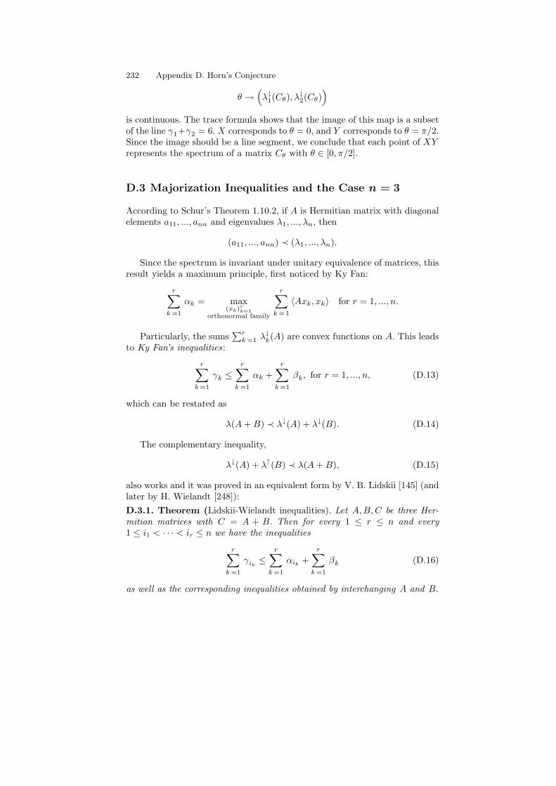
232 Appendix D. Horn’s Conjecture
θ →(λ↓1(Cθ), λ
↓2(Cθ)
)
is continuous. The trace formula shows that the image of this map is a subsetof the line γ1+γ2 = 6. X corresponds to θ = 0, and Y corresponds to θ = π/2.Since the image should be a line segment, we conclude that each point of XYrepresents the spectrum of a matrix Cθ with θ ∈ [0, π/2].
D.3 Majorization Inequalities and the Case n = 3
According to Schur’s Theorem 1.10.2, if A is Hermitian matrix with diagonalelements a11, ..., ann and eigenvalues λ1, ..., λn, then
(a11, ..., ann) ≺ (λ1, ..., λn).
Since the spectrum is invariant under unitary equivalence of matrices, thisresult yields a maximum principle, first noticed by Ky Fan:
r∑
k =1
αk = max(xk)r
k=1orthonormal family
r∑
k = 1
〈Axk, xk〉 for r = 1, ..., n.
Particularly, the sums∑r
k =1 λ↓k(A) are convex functions on A. This leadsto Ky Fan’s inequalities:
r∑
k =1
γk ≤r∑
k =1
αk +r∑
k =1
βk, for r = 1, ..., n, (D.13)
which can be restated as
λ(A + B) ≺ λ↓(A) + λ↓(B). (D.14)
The complementary inequality,
λ↓(A) + λ↑(B) ≺ λ(A + B), (D.15)
also works and it was proved in an equivalent form by V. B. Lidskii [145] (andlater by H. Wielandt [248]):D.3.1. Theorem (Lidskii-Wielandt inequalities). Let A,B,C be three Her-mitian matrices with C = A + B. Then for every 1 ≤ r ≤ n and every1 ≤ i1 < · · · < ir ≤ n we have the inequalities
r∑
k =1
γik≤
r∑
k =1
αik+
r∑
k =1
βk (D.16)
as well as the corresponding inequalities obtained by interchanging A and B.
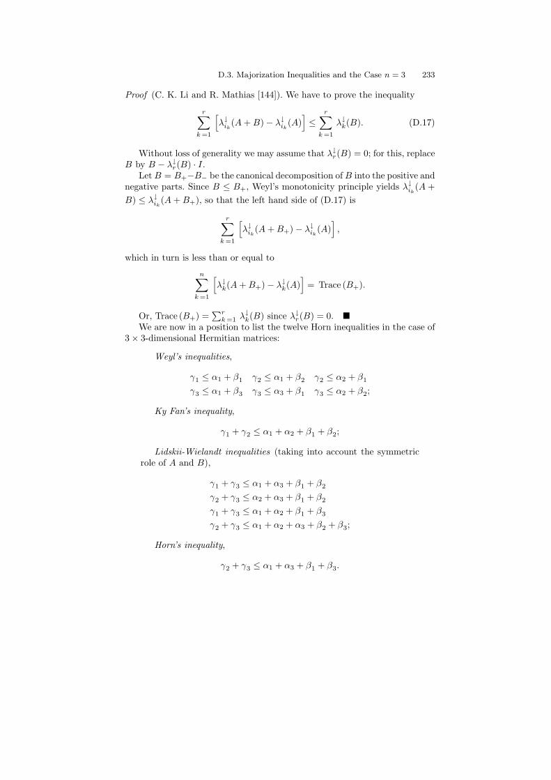
D.3. Majorization Inequalities and the Case n = 3 233
Proof (C. K. Li and R. Mathias [144]). We have to prove the inequality
r∑
k =1
[λ↓ik
(A + B)− λ↓ik(A)
]≤
r∑
k =1
λ↓k(B). (D.17)
Without loss of generality we may assume that λ↓r(B) = 0; for this, replaceB by B − λ↓r(B) · I.
Let B = B+−B− be the canonical decomposition of B into the positive andnegative parts. Since B ≤ B+, Weyl’s monotonicity principle yields λ↓ik
(A +B) ≤ λ↓ik
(A + B+), so that the left hand side of (D.17) is
r∑
k =1
[λ↓ik
(A + B+)− λ↓ik(A)
],
which in turn is less than or equal to
n∑
k =1
[λ↓k(A + B+)− λ↓k(A)
]= Trace (B+).
Or, Trace (B+) =∑r
k =1 λ↓k(B) since λ↓r(B) = 0. ¥We are now in a position to list the twelve Horn inequalities in the case of
3× 3-dimensional Hermitian matrices:
Weyl’s inequalities,
γ1 ≤ α1 + β1 γ2 ≤ α1 + β2 γ2 ≤ α2 + β1
γ3 ≤ α1 + β3 γ3 ≤ α3 + β1 γ3 ≤ α2 + β2;
Ky Fan’s inequality,
γ1 + γ2 ≤ α1 + α2 + β1 + β2;
Lidskii-Wielandt inequalities (taking into account the symmetricrole of A and B),
γ1 + γ3 ≤ α1 + α3 + β1 + β2
γ2 + γ3 ≤ α2 + α3 + β1 + β2
γ1 + γ3 ≤ α1 + α2 + β1 + β3
γ2 + γ3 ≤ α1 + α2 + α3 + β2 + β3;
Horn’s inequality,
γ2 + γ3 ≤ α1 + α3 + β1 + β3.
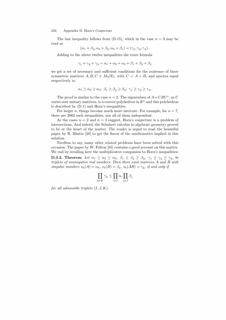
234 Appendix D. Horn’s Conjecture
The last inequality follows from (D.15), which in the case n = 3 may beread as
(α1 + β3, α2 + β2, α3 + β1) ≺ (γ1, γ2, γ3) .
Adding to the above twelve inequalities the trace formula
γ1 + γ2 + γ3 = α1 + α2 + α3 + β1 + β2 + β3
we get a set of necessary and sufficient conditions for the existence of threesymmetric matrices A, B,C ∈ M3(R), with C = A + B, and spectra equalrespectively to
α1 ≥ α2 ≥ α3; β1 ≥ β2 ≥ β3; γ1 ≥ γ2 ≥ γ3.
The proof is similar to the case n = 2. The eigenvalues of A+UBU?, as Uvaries over unitary matrices, is a convex polyhedron in Rn and this polyhedronis described by (D.1) and Horn’s inequalities.
For larger n, things become much more intricate. For example, for n = 7,there are 2062 such inequalities, not all of them independent.
As the cases n = 2 and n = 3 suggest, Horn’s conjecture is a problem ofintersections. And indeed, the Schubert calculus in algebraic geometry provedto be at the heart of the matter. The reader is urged to read the beautifulpaper by R. Bhatia [28] to get the flavor of the mathematics implied in thissolution.
Needless to say, many other related problems have been solved with thisoccasion. The paper by W. Fulton [85] contains a good account on this matter.We end by recalling here the multiplicative companion to Horn’s inequalities:D.3.2. Theorem. Let α1 ≥ α2 ≥ α3, β1 ≥ β2 ≥ β3, γ1 ≥ γ2 ≥ γ3, betriplets of nonnegative real numbers. Then there exist matrices A and B withsingular numbers sk(A) = αk, sk(B) = βk, sk(AB) = γk, if and only if
∏
k∈K
γk ≤∏
i∈I
αi
∏
j∈J
βj
for all admissible triplets (I, J,K).
References
1. S. Abramovich, G. Jameson and G. Sinnamon, Refining Jensen’sInequality. Bull. Math. Soc. Sc. Math. Roumanie. To appear.
2. J. Aczel, The notion of mean values, Norske Vid. Selsk. Forhdl.,Trondhjem, 19 (1947), 83-86.
3. J. Aczel, A Generalization of the Notion of Convex Functions,Norske Vid. Selsk. Forhdl., Trondhjem, 19 (1947), 87-90.
4. G. Alberti and L. Ambrosio, A geometrical approach to monotonefunctions in Rn, Math. Z., 230 (1999), 259-316.
5. A. D. Alexandrov, Almost everywhere existence of the second differ-ential of a convex function and some properties of convex surfacesconnected to it, Leningrad State Univ. Ann., Math. Ser. 6 (1939),3-35. (Russian)
6. E. M. Alfsen, Compact convex sets and boundary integrals, Springer-Verlag, Berlin, 1971.
7. H. W. Alt, Lineare Funktionalanalysis. Eine anwendungsorientierteEinfuhrung, 2 Auflage, Springer-Verlag, 1992.
8. H. Alzer, On an integral inequality, Math. Rev. Anal. Numer. Th.Approx., 18 (1989), 101-103.
9. T. Ando, C.-K. Li and R. Mathias, Geometric Means. Linear AlgebraAppl., 385 (2004), 305-334.
10. G. Andrews, R. Askey and R. Roy, Special Functions, CambridgeUniversity Press, 1999.
11. E. Artin, The Gamma Function, Holt, Rinehart and Winston, NewYork, 1964. English translation of German original, Einfuhrung indie Theorie der Gammafunktion, Teubner, 1931.
12. E. Asplund, Frechet differentiability of convex functions, Acta Math.,121 (1968), 31-47.
13. M. Atiyah, Angular momentum, convex polyhedra and algebraic ge-ometry, Proc. Edinburgh Math. Soc., 26 (1983), 121-138.
14. G. Aumann, Konvexe Funktionen und die Induktion bei Ungleichun-gen swischen Mittelwerten, S.-B. math.-naturw. Abt. Bayer. Akad.Wiss. Munchen (1933), 403-415.
15. V. Barbu and Th. Precupanu, Convexity and Optimization in Ba-nach Spaces, Ed. Academiei, Bucharest, and D. Reidel Publ. Co.,Dordrecht, 1986.

236 References
16. F. Barthe, Inegalites de Brascamp-Lieb et convexite, C. R. Acad. Sci.Paris, Serie I, t. 324 (1997), 885-887.
17. F. Barthe, Optimal Young’s Inequality and Its Converse: A SimpleProof, Geom. Funct. Anal., 8 (1998), 234-242.
18. S. Barza and C. P. Niculescu, Integral Inequalities for Concave Func-tions. Preprint, 2004.
19. E. F. Beckenbach and R. Bellman, Inequalities, Springer-Verlag,Berlin, 2nd Ed., 1983.
20. R. Benedetti and J.-J. Risler, Real algebraic and semi-algebraic sets,Hermann, Editeurs des Sciences et des Arts, Paris, 1990.
21. C. Bennett and R. Sharpley, Interpolation of Operators, AcademicPress, 1988.
22. G. Berkhan, Zur projektivischen Behandlung der Dreiecksgeometrie,Arch. Math. Phys., (3) 11 (1907), 1-31.
23. J. Bernoulli, Positiones Arithmeticae de seriebus infinitas, earumquesumma finita, Basileae, 1689, Opera 1, p. 375-402.
24. M. Berger, Convexity, Amer. Math. Monthly, 97 (1990), 650-678.25. L. Berwald, Verallgemeinerung eines Mittelwertsatzes von J.
Favard, fur positive konkave Funktionen, Acta Math., 79 (1947),17-37.
26. M. Bessenyei and Z. Pales, Higher order generalizations ofHadamard’s inequality, Publ. Math. Debrecen, 61 (2002), 623-643.
27. M. Bessenyei and Z. Pales, Hadamard-type inequalities for general-ized convex functions, Math. Inequal. Appl., 6 (2003), 379-392.
28. R. Bhatia, Linear Algebra to Quantum Cohomology: The Story ofAlfred Horn’s Inequalities, Amer. Math. Monthly, 108 (2001), 289-318.
29. G. Bianchi, A. Colesanti and C. Pucci, On the Second Differentia-bility of Convex Surfaces, Geometriae Dedicata, 60 (1996), 39-48.
30. Z. W. Birnbaum and W. Orlicz, Uber die Verallgemeinerung desBegriffes der zueinander konjugierten Potenzen, Studia Math., 3(1931), 1-67.
31. E. Bishop and K. de Leeuw, The representation of linear functionalsby measures on sets of extreme points, Ann. Inst. Fourier (Grenoble),9 (1959), 305-331.
32. H. Blumberg, On convex functions, Trans. Amer. Math. Soc., 20(1919), 40-44.
33. H. Bohr and J. Mollerup, Laerebog i Mathematisk Analyse III,Kopenhagen, 1922.
34. Ch. Borell, Convex set functions in d-space, Period. Math. Hungar.,6 (1975), 111-136.
35. Ch. Borell, Diffusion Equations and Geometric Inequalities, Poten-tial Analysis, 12 (2000), 49-71.
36. D. Borwein, J. Borwein, G. Fee and R. Girgensohn, Refined convexityand special cases of the Blaschke-Santalo inequality, Math. Inequal.Appl., 4 (2001), 631-638.
37. J. Borwein, Continuity and differentiability properties of convex op-erators, Proc. London Math. Soc., 44 (1982), 420-444.
38. J. M. Borwein and P. B. Borwein, The Way of All Means, Amer.Math. Monthly, 94 (1987), 519-522.
References 237
39. J. M. Borwein and A. S. Lewis, Convex Analysis and Nonlinear Op-timization. Theory and Examples., Springer-Verlag, Berlin, 2000.
40. H. J. Brascamp and E. H. Lieb, Best constants in Young’s inequal-ity, its converse and its generalization to more than three functions,Advances in Math., 20 (1976), 151-173.
41. H. J. Brascamp and E. H. Lieb, On Extensions of the Brunn-Minkowski and Prekopa-Leindler Theorems, Including Inequalitiesfor Log Concave Functions, and with an Application to the DiffusionEquation, Functional Analysis, 22 (1976), 366-389.
42. Y. Brenier, Polar Factorization and Monotone Rearrangemenent ofVector-Valued Functions, Commun. on Pure and Appl. Math. XLIV(1991), 375-417.
43. J. L. Brenner and B. C. Carlson, Homogeneous mean values: weightsand asymptotics, J. Math. Anal. Appl., 123 (1987), 265-280.
44. H. Brezis, Operateurs Maximaux Monotones et semigroups de con-tractions dans les espaces de Hilbert, North Holland, Amsterdam,1973.
45. P. S. Bullen, D. S. Mitrinovic and P. M. Vasic, Means and TheirInequalities, D. Reidel Publishing Company, Dordrecht, 1988.
46. Y. D. Burago and V. A. Zalgaller, Geometric Inequalities, Springer-Verlag, New York, 1988
47. F. Burk, The Geometric, Logarithmic and Arithmetic Mean Inequal-ity, Amer. Math. Monthly, 94 (1987), 527-528.
48. G. T. Cargo, Comparable means and generalized convexity, J. Math.Anal. Appl., 12 (1965), 387-392.
49. T. Carleman, Sur les fonctions quasi-analitiques. In Comptes Ren-dus du V-e Congres des Mathematiciens Scandinaves, Helsingfors,Finland, 1922, 181-196.
50. B. C. Carlson, Algorithms involving arithmetic and geometric means,Amer. Math. Monthly, 78 (1971), 496–505.
51. A.-L. Cauchy, Cours d’analyse de l’Ecole Royale Polytechnique, 1erepartie, Analyse algebrique, Paris, 1821. See also, Œuvres completes,IIe serie, VII.
52. J. Cea, Optimisation. Theorie et Algorithmes, Dunod, Paris, 1971.53. S. H. Chang, On the distribution of the characteristic values and
singular values of linear integral equations, Trans. Amer. Math. Soc.,67 (1949), 351-67.
54. G. Choquet, Les cones convexes faiblement complets dans l’Analyse,Proc. Intern. Congr. Mathematicians, Stockholm (1962), 317-330.
55. A. Cizmesija and J. E. Pecaric, Mixed means and Hardy’s inequality,Math. Inequal. Appl., 1 (1998), 491-506.
56. A. Cizmesija and J. E. Pecaric and L.-E. Persson, On strength-ened Hardy and Polya-Knopp’s inequalities, J. Approx. Theory, 125(2003), 74-84.
57. F. H. Clarke, Optimization and Nonsmooth Analysis, 2nd Edition,Classics in Applied Mathematics, vol. 5, Society for Industrial andApplied Mathematics (SIAM), Philadelphia, PA, 1990.
58. J. A. Clarkson, Uniformly convex spaces, Trans. Amer. Math. Soc.,40 (1936), 396-414.
238 References
59. J. B. Conway, A Course in Functional Analysis, 2nd Ed., Springer-Verlag, Berlin, 1997.
60. D. Cordero-Erausquin, R. J. McCann and M. Schmuckenschlager, ARiemannian interpolation inequality a la Borell, Brascamp and Lieb,Invent. Math., 146 (2001), 219-257.
61. D. Cordero-Erausquin, Some Applications of Mass Transport toGaussian-Type Inequalities, Arch. Rational Mech. Anal., 161 (2002),257-269.
62. M. G. Crandall, H. Ishii and P.-L. Lions, User’s guide to viscositysolutions of second order partial differential equations, Bull. Amer.Math. Soc., 27 (1992), 1-67.
63. S. Dancs and B. Uhrin, On a class of integral inequalities and theirmeasure-theoretic consequences, J. Math. Anal. Appl.,74 (1980),388-400.
64. K. R. Davidson and A. P. Donsig, Real Analysis with Real Applica-tions, Prentice Hall, Upper Saddle River, N.J., 2002.
65. M. M. Day, Normed linear spaces, 3rd Edition, Springer-Verlag,Berlin, 1973.
66. J. B. Diaz and F. T. Metcalf, Stronger forms of a class of inequalitiesof G. Polya-G. Szego, and L. V. Kantorovich, Bull. Amer. Math.Soc., 69 (1963), 415-418.
67. J. Dieudonne, Foundations of Modern Analysis, Academic Press,1960.
68. S. S. Dragomir and N. M. Ionescu, Some converse of Jensen’s in-equality and applications, Rev. Anal. Numer. Theor. Approx. 23(1994), 71-78.
69. J. Duncan and C. M. McGregor, Carleman’s inequality, Amer. Math.Monthly, 110 (2003), 424-431.
70. G. Duvaut and J. L. Lions, Inequalities in Mechanics and Physics,Springer-Verlag, Berlin, 1976.
71. I. Ekeland and R. Temam, Convex Analysis and Variational Prob-lems, North-Holland Publishing Company, Amsterdam, 1976.
72. N. Elezovic and J. Pecaric, Differential and integral F -means andapplications to digamma function, Math. Inequal. Appl., 3 (2000),189-196.
73. A. Engel, Problem Solving Strategies, Springer-Verlag, Berlin, 1998.74. Euclid, The thirteen books of Euclid’s Elements (translated by Sir
Thomas Heath, Cambridge, 1908).75. L. C. Evans and R. F. Gariepy, Measure Theory and Fine Proper-
ties of Functions, CRC Press, Boca Raton·New York·London·Tokyo,1992.
76. K. Fan, On a theorem of Weyl concerning eigenvalues of linear trans-formations II, Proc. Nat. Acad. Sci. U.S.A., 36 (1950), 31-35.
77. J. Favard, Sur les valeurs moyennes, Bull. Sci. Math., 57 (1933),54-64.
78. H. Federer, Geometric Measure Theory, Springer-Verlag, New York,1969.
79. W. Fenchel, On conjugate convex functions, Canad. J. Math., 1(1949), 73-77.

References 239
80. W. Fenchel, Convex Cones, Sets and Functions (mimeographed lec-ture notes). Princeton Univ. Press, Princeton, 1951.
81. B. de Finetti, Sul concetto di media, Giornale dell’ Instituto Italianodegli Attuari, 2 (1931), 369-396.
82. A. M. Fink, A best possible Hadamard inequality, Math. Inequal.Appl., 1 (1998), 223-230.
83. J. Franklin, Mathematical Methods of Economics, Amer. Math.Monthly, 90 (1983), 229-244.
84. L. Fuchs, A new proof of an inequality of Hardy, Littlewood andPolya, Mat. Tidsskr. B., 1947, 53-54.
85. W. Fulton, Eigenvalues, invariant factors, highest weights and Schu-bert calculus. Bull. Amer. Math. Soc., 37 (2000), 209-249.
86. D. Gale, V. Klee and R. T. Rockafellar, Convex functions on convexpolytopes, Proc. Amer. Math. Soc., 19 (1968), 867-873.
87. L. Galvani, Sulle funzioni converse di una o due variabili definite inaggregate qualunque, Rend. Circ. Mat. Palermo, 41 (1916), 103-134.
88. R. J. Gardner, The Brunn-Minkowski inequality : A survey withproofs. Preprint, 2001. Available at http://www.ac.wwu.edu/
89. R. J. Gardner, The Brunn-Minkowski inequality, Bull. Amer. Math.Soc., 39 (2002), 355-405.
90. I. S. Gradshteyn and I. M. Ryzhik, Table of Integrals, Series andProducts, Academic Press, 1996. (CD-ROM version)
91. D. Gronau and J. Matkowski, Geometrical convexity and generaliza-tions of the Bohr-Mollerup theorem on the Gamma function, Math-ematica Panonica, 4 (1993), 153-160.
92. D. Gronau and J. Matkowski, Geometrically convex solutions of cer-tain difference equations and generalized Bohr-Mollerup type theo-rems, Results in Mathematics, 26 (1994), 290-297.
93. P. M. Gruber, Aspects of convexity and its applications, Expo. Math.,2 (1984), 47-83.
94. P. M. Gruber and J. M. Willis (eds), Handbook of convex geometry,North-Holland, Amsterdam, 1993.
95. J. Hadamard, Etude sur les proprietes des fonctions entieres et enparticulier d’une fonction consideree par Riemann, J. Math. Pureset Appl., 58 (1893), 171-215.
96. G. Hamel, Eine Basis aller Zahlen und die unstetigen Losungen derFunktionalgleichung f(x+y) = f(x)+ f(y), Math. Ann., 60 (1905),459-462.
97. O. Hanner, On the uniform convexity of Lp and lp, Ark. Mat., 3(1955), 239-244.
98. G. H. Hardy, A note on two inequalities, J. London Math. Soc., 11(1936), 167-170.
99. G. H. Hardy, J. E. Littlewood and G. Polya, Some simple inequalitiessatisfied by convex functions, Messenger Math., 58 (1929), 145-152.
100. G. H. Hardy, J. E. Littlewood and G. Polya, Inequalities, CambridgeMathematical Library, 2nd Edition, 1952, Reprinted 1988.
101. H. Heinig and L. Maligranda, Weighted inequalities for monotoneand concave functions, Studia Math., 116 (1995), 133-165.
240 References
102. R. Henstock and A. M. Macbeath, On the measure of sum sets I. Thetheorems of Brunn, Minkowski and Lusternik, Proc. London Math.Soc., 3 (1953), 182-194.
103. Ch. Hermite, Sur deux limites d’une integrale definie, Mathesis, 3(1883), p. 82.
104. E. Hewitt and K. Stromberg, Real and Abstract Analysis, Springer-Verlag, Berlin, 1965.
105. J.-B. Hiriart-Urruty and C. Lemarechal, Convex Analysis and Min-imization Algorithms, Springer-Verlag, Berlin, 1993.
106. J.-B. Hiriart-Urruty, Ensembles de Tchebychev vs ensembles con-vexes: l’etat de la situation vu via l’analyse non lisse, Ann. Sci. Math.Quebec, 22 (1998), 47-62.
107. O. Holder, Uber einen Mittelwertsatz, Nachr. Ges. Wiss. Goettingen,1889, 38-47.
108. L. Hormander, Sur la fonction d’appui des ensembles convexes dansune espace localement convexe, Ark. Mat., 3 (1954), 181-186.
109. L. Hormander, Notions of Convexity, Birkhauser, Boston, 1994.110. A. Horn, Doubly stochastic matrices and the diagonal of a rotation
matrix, Amer. J. Math., 76 (1954), 620-630.111. A. Horn, On the eigenvalues of a matrix with prescribed singular
values, Proc. Amer. Math. Soc., 5 (1954), 4-7.112. A. Horn, Eigenvalues of Sums of Hermitian matrices, Pacific J.
Math., 12 (1962), 225-241.113. H. Hornich, Eine Ungleichung fur Vektorlangen, Math. Z., 48 (1942),
268-273.114. K. S. K. Iyengar, Note on an inequality, Math. Student, 6 (1938),
75-76.115. J. L. W. V. Jensen, Om konvexe Funktioner og Uligheder mellem
Middelvaerdier, Nyt. Tidsskr. Math., 16B (1905), 49-69.116. J. L. W. V. Jensen, Sur les fonctions convexes et les inegalites entre
les valeurs moyennes, Acta Math., 30 (1906), 175-193.117. M. Johansson, L.-E. Persson and A. Wedestig, Carleman’s inequality-
history, proofs and some new generalizations, J. Inequal. Pure Appl.Math. (JIPAM) 4 (2003), no. 3, article 53.
118. K. Jorgens, Linear Integral Operators, Pitman Advanced PublishingProgram, Boston, 1982.
119. B. Josefson, Weak sequential convergence in the dual of a Banachspace does not imply norm convergence, Ark. Mat., 13 (1975), 79-89.
120. S. Kaijser, L.-E. Persson and A. Oberg, On Carleman and Knopp’sinequalities, J. Approx. Theory, 117 (2002), 140-151.
121. J. Karamata, Sur une inegalite relative aux fonctions convexes, Publ.Math. Univ. Belgrade, 1 (1932), 145-148.
122. N. D. Kazarinoff, Analytic Inequalities, Holt, Rinehart and Winston,New York, 1961.
123. B. Kawohl, When are superharmonic functions concave? Applica-tions to the St. Venant torsion problem and to the fundamental modeof the clamped membrane, Z. Angew. Math. Mech. 64 (1984), 364-366.

References 241
124. B. Kawohl, Rearrangements and Convexity of Level Sets in PDE,Lecture Notes in Mathematics, No. 1150, Springer-Verlag, 1985.
125. K. Kedlaya, Proof of a Mixed Arithmetic-Mean, Geometric-MeanInequality, Amer. Math. Monthly, 101 (1994), 355-357.
126. J. L. Kelley, General Topology, D. van Nostrand Company, Prince-ton, 1957.
127. L. G. Khanin, Problem M 1083, Kvant, 18 (1988), No. 1, p. 35 andKvant, 18 (1988), No. 5, p. 35.
128. C. H. Kimberling, Some Corollaries to an Integral Inequality, Amer.Math. Monthly, 81 (1974), 269-270.
129. M. S. Klamkin, Inequalities for inscribed and circumscribed polygons,Amer. Math. Monthly, 87 (1980), 469-473.
130. V. Klee, Some new results on smoothness and rotundity in normedlinear spaces, Math. Ann., 139 (1959), 51-63.
131. A. A. Klyachko, Stable bundles, representation theory and Hermitianoperators, Selecta Math., 4 (1998), 419-445.
132. K. Knopp, Uber Reihen mit positiven Gliedern, J. London Math.Soc., 3 (1928), 205-211.
133. A. Knutson and T. Tao, The honeycomb model of GLn(C) tensorproducts I: Proof of the saturation conjecture, J. Amer. Math. Soc.,12 (1999), 1055-1090.
134. M. A. Krasnosel’skii and Ya. B. Rutickii, Convex Functions and Or-licz Spaces, P. Nordhoff, Groningen, 1961.
135. J. L. Krivine, Theoremes de factorisation dans les espaces reticules,Seminaire Maurey-Schwartz, 1973-74, Exposes 22-23, Ecole Poly-technique, Paris.
136. F. Kubo and T. Ando, Means of Positive Linear Operators, Math.Ann., 246, 205-224 (1980).
137. A. Kufner and L.-E. Persson, Weighted Inequalities of Hardy Type,World Scientific, New Jersey/London/Singapore/Hong Kong, 2003.
138. J. Lamperti, On the isometries of certain function-spaces, Pacific J.Math., 8 (1958), 459-466.
139. S. Lang, Analysis I, Addison-Wesley Publ. Co., Reading, Mas-sachusetts, 1968.
140. S. Lang, Analysis II, Addison-Wesley Publ. Co., Reading, Mas-sachusetts, 1969.
141. J. M. Lasry and P.-L. Lions, A remark on regularization in Hilbertspaces, Israel. J. Math., 55 (1986), 257-266.
142. J. D. Lawson and Y. Lim, The Geometric Mean, Matrices, Metricsand More, Amer. Math. Monthly, 108, 797-812 (2001).
143. V. I. Levin and S. B. Steckin, Inequalities, Amer. Math. Soc. Transl.,14 (1960), 1-22.
144. C.-K. Li and R. Mathias, The Lidskii-Mirsky-Wielandt theorem -additive and multiplicative versions, Numer. Math., 81 (1999), 377-413.
145. V. B. Lidskii, The proper values of the sum and product of symmetricmatrices, Dokl. Akad. Nauk S.S.S.R., 74 (1950), 769-772.
146. E. H. Lieb and M. Loss, Analysis, 2nd Edition, Amer. Math. Soc.,Providence, R. I., 2001.

242 References
147. T.-P. Lin, The power mean and the logarithmic mean, Amer. Math.Monthly, 81 (1974), 879-883.
148. J. Lindenstrauss and A. PeÃlczynski, Absolutely summing operatorsin Lp-spaces and their applications, Studia Math. XXIX (1968),275-326.
149. J. Lindenstrauss and L. Tzafriri, Classical Banach spaces, Vol. 1(1977), Vol. 2 (1979), Springer-Verlag, Berlin.
150. A. Lyapunov, Nouvelle forme du theoreme sur la limite de proba-bilite, Memoires de l’Acad. de St.-Petersburg, (VIII) 12 (1901), no.5, 1-24.
151. C. Maclaurin, A second letter to Martin Folkes, Esq.; concerning theroots of equations, with the demonstration of other rules in algebra,Phil. Transactions, 36 (1729), 59-96.
152. S. M. Malamud, Some complements to the Jensen and Chebyshevinequality and a problem of W. Walter, Proc. Amer. Math. Soc.,129 (2001), 2671-2678.
153. L. Maligranda, Concavity and convexity of rearrangements, Com-ment. Math. Prace, 32 (1992), 85-90.
154. L. Maligranda, Why Holder’s inequality should be called Rogers’ in-equality?, Math. Inequal. Appl., 1 (1998), 69-83.
155. L. Maligranda, J. E. Pecaric and L.-E. Persson, On Some Inequalitiesof the Gruss-Barnes and Borell Type, J. Math. Anal. and Appl., 187(1994), 306-323.
156. M. Marcus and J. Lopes, Inequalities for symmetric functions andHermitian matrices, Canad. J. Math., 8 (1956), 524-531.
157. A. W. Marshall and I. Olkin, Inequalities: Theory of Majorizationand its Applications, Academic Press, 1979.
158. M. Matic and J. E. Pecaric, Some companion inequalities to Jensen’sinequality, Math. Inequal. Appl., 3 (2000), 355-368.
159. J. Matkowski, Convex and affine functions with respect to a meanand a characterization of the weighted quasi-arithmetic means, RealAnalysis Exchange, to appear.
160. J. Matkowski and J. Ratz, Convexity of power functions with re-spect to symmetric homogeneous means, Int. Ser. Numer. Math., 123(1997), 231-247.
161. J. Matkowski and J. Ratz, Convex functions with respect to an arbi-trary mean, Int. Ser. Numer. Math., 123 (1997), 249-258.
162. S. Mazur and S. Ulam, Sur les transformations isometriquesd’espaces vectoriels normes, C. R. Acad. Sci. Paris, 194, 946-948(1932).
163. R. J. McCann, Existence and uniqueness of monotone measure-preserving maps, Duke Math. J., 80 (1995), 309-323.
164. R. J. McCann, A convexity principle for interacting gases, Adv.Math., 128 (1997), 153-179.
165. F. Mignot, Controle dans les Inequations Variationelles Elliptiques,J. Funct. Anal., 22 (1976), 130-185.
166. H. Minkowski, Theorie der Konvexen Korper, InsbesondereBegrundung ihres Oberflachenbegriffs, Gesammelte AbhandlungenII, Leipzig, 1911.

References 243
167. G. Minty, Monotone nonlinear operators on a Hilbert space, DukeMath. J., 29 (1962), 341-346.
168. D. S. Mitrinovic, Analytic Inequalities, Springer-Verlag, Berlin andNew York, 1970.
169. D. S. Mitrinovic and I. B. Lackovic, Hermite and convexity, Aequa-tiones Math., 28 (1985), 229-232.
170. D. S. Mitrinovic, J. E. Pecaric and A. M. Fink, Inequalities InvolvingFunctions and Their Integrals and Derivatives, Kluwer AcademicPubl., Dordrecht, 1991.
171. D. S. Mitrinovic and P. M. Vasic, History, variations and generaliza-tions of the Cebysev inequality and the question of some priorities,Univ. Beograd. Publ. Elektrotehn. Fak. Ser. Mat. Fiz. No. 461, 1974,1-30.
172. B. Mond and J. E. Pecaric, A Mixed Means Inequality, Austral.Math. Soc. Gazette, 23 (1996), 67-70.
173. P. Montel, Sur les functions convexes et les fonctions soushar-moniques, Journal de Math., (9), 7 (1928), 29-60.
174. R. F. Muirhead, Some methods applicable to identities and inequal-ities of symmetric algebraic functions of n letters, Proc. EdinburghMath. Soc., 21 (1903), 144-157.
175. J. Nash, Non-cooperative games, Ann. of Math. 54 (1951), 286-295.176. T. Needham, A visual explanation of Jensen’s Inequality, Amer.
Math. Monthly, 100 (1993), 768-771.177. E. Neuman and J. Sandor, On the Ky Fan inequality and related
inequalities I, Math. Inequal. Appl., 5 (2002), 49-56.178. I. Newton, Arithmetica universalis : sive de compositione et resolu-
tione arithmetica liber, 1707.179. C. P. Niculescu, Convexity according to the geometric mean, Math.
Inequal. Appl., 3 (2000), 155-167.180. C. P. Niculescu, A new look at Newton’s Inequalities, J. Inequal. Pure
Appl. Math. (JIPAM), 1 (2000), no. 2, article 17.181. C. P. Niculescu, A multiplicative mean value and its applications. In:
Inequality Theory and Applications, Vol. 1, 243-255, Nova SciencePublishers, Huntington, New York, 2001 (Y. J. Cho, S. S. Dragomirand J. Kim, Editors).
182. C. P. Niculescu, An extension of Chebyshev’s inequality and its con-nection with Jensen’s inequality, J. Inequal. Appl., 6 (2001), no. 4,451-462.
183. C. P. Niculescu, A note on the Hermite-Hadamard Inequality, TheMathematical Gazette, July 2001, 48-50.
184. C. P. Niculescu, Choquet theory for signed measures, Math. Inequal.Appl., 5 (2002), 479-489.
185. C. P. Niculescu, The Hermite-Hadamard inequality for functions ofseveral variables, Math. Inequal. Appl., 5 (2002), 619-623.
186. C. P. Niculescu, Convexity according to means, Math. Inequal. Appl.,6 (2003), 571-579.
187. C. P. Niculescu, An extension of the Mazur-Ulam Theorem, Proc.Intern. Workshop on Global Analysis, Ankara, April 15-17, 2004.
188. C. P. Niculescu, Interpolating Newton’s Inequalities, Bull. Math. Soc.Sc. Math. Roumanie, 47 (95), No. 1-2, 2004.

244 References
189. C. P. Niculescu and L.-E. Persson, Old and New on the Hermite-Hadamard Inequality, Real Anal. Exchange, to appear.
190. C. P. Niculescu and F. Popovici, A Note on the Denjoy-BourbakiTheorem, Real Anal. Exchange, to appear.
191. C. P. Niculescu and F. Popovici, A Refinement of Popoviciu’s In-equality, Math. Inequal. Appl., to appear.
192. C. P. Niculescu and F. Popovici, The Extension of MajorizationInequalities within the Framework of Relative Convexity. Preprint,2004.
193. L. Nikolova, L.-E. Persson and T. Zachariades, On Clarkson’s In-equality, Type and Cotype of Edmunds-Triebel Logarithmic Spaces,Arch. Math. 80 (2003), 165-176.
194. B. Opic and A. Kufner, Hardy Type Inequalities, Longman, Harlow,1990.
195. R. Osserman, Curvature in the Eighties, Amer. Math. Monthly, 97(1990), 731-756.
196. A. M. Ostrowski, Sur quelques applications des fonctions convexes etconcaves au sens de I. Schur, J. Math. Pures Appl., (9) 31 (1952),253-292.
197. J. E. Pecaric, A simple proof of the Jensen-Steffensen inequality,Amer. Math. Monthly, 91 (1984), 195-196.
198. J. E. Pecaric, F. Proschan and Y. C. Tong, Convex functions, PartialOrderings and Statistical Applications, Academic Press, New York,1992.
199. J. E. Pecaric and V. Simic, Stolarski-Tobey mean in n variables,Math. Inequal. Appl., 2 (1999), 325-341.
200. J. E. Pecaric and K. B. Stolarsky, Carleman’s inequality: history andnew generalizations, Aequationes Math., 61 (2001), 49-62.
201. R. R. Phelps, Convex functions, Monotone Operators, and Differen-tiability, 2nd Edition, Lecture Notes in Math. No. 1364, Springer-Verlag, Berlin, 1993.
202. R. R. Phelps, Lectures on Choquet’s Theorem, 2nd Edition, LectureNotes in Math. No. 1757, Springer-Verlag, Berlin, 2001.
203. A. O. Pittenger, The logarithmic mean in n variables, Amer. Math.Monthly, 92 (1985), 99-104.
204. G. Polya, Mathematics and Plausible Reasoning, Vols. I & II, Prince-ton Univ. Press., Princeton, New Jersey, 1954.
205. G. Polya and G. Szego, Aufgaben und Lehrsatze aus Analysis, Vols. I& II, Springer-Verlag, 1925. English edition, Springer-Verlag, 1972.
206. T. Popoviciu, Sur quelques proprietes des fonctions d’une ou de deuxvariables reelles, Mathematica (Cluj), 8 (1934), 1-85.
207. T. Popoviciu, Notes sur les fonctions convexes d’ordre superieur(IX), Bull. Math. Soc. Roum. Sci., 43 (1941), 85-141.
208. T. Popoviciu, Les Fonctions Convexes, Hermann, Paris, 1944.209. T. Popoviciu, Sur certaines inegalites qui caracterisent les fonctions
convexes, Analele Stiintifice Univ. ”Al. I. Cuza”, Iasi, Sectia Mat.,11 (1965), 155-164.
210. W. Pusz and S. L. Woronowicz, Functional calculus for sesquilinearforms and the purification map, Rep. Math. Phys., 8, 159-170 (1975).
References 245
211. R. Rado, An inequality, J. London Math. Soc., 27 (1952), 1-6.212. M. M. Rao and Z. D. Ren, Theory of Orlicz Spaces, Marcel Dekker,
1991.213. M. Radulescu and S. Radulescu, Generalization of Dobrusin’s In-
equalities and Applications, J. Math. Anal. Appl. 204 (1996), 631-645.
214. M. Renardy and R. C. Rogers, An Introduction to Partial DifferentialEquations, Springer-Verlag, Berlin, 1993.
215. A. W. Roberts and D. E. Varberg, Convex Functions, AcademicPress, New York and London, 1973.
216. R. T. Rockafellar, Convex Analysis, Princeton Math. Ser. No. 28,Princeton Univ. Press, Princeton, New Jersey, 1970.
217. G. Rode, Eine abstrakte Version des Satzes von Hahn-Banach, Arch.Math. (Basel) 31 (1978), 474-481.
218. L. J. Rogers, An extension of a certain theorem in inequalities, Mes-senger of Math., 17 (1888), 145-150.
219. P. Roselli and M. Willem, A convexity inequality, Amer. Math.Monthly, 109 (2002), 64-70.
220. S. Rosset, Normalized symmetric functions, Newton’s inequalitiesand a new set of stronger inequalities, Amer. Math. Monthly, 96(1989), 815-819.
221. W. Rudin, Real and Complex Analysis, 3rd Ed., Mc Graw-Hill, NewYork, 1987.
222. S. Saks, Sur un theoreme de M. Montel, C. R. Acad. Sci. Paris, 187(1928), 276-277.
223. T. Sasaki, Y. Kanada and S. Watanabe, Calculation of discriminantsof higher degree equations, Tokyo J. Math., 4 (1981), 493-503.
224. R. A. Satnoianu, Erdos-Mordell-Type Inequalities in a Triangle,Amer. Math. Monthly, 110 (2003), 727-729.
225. I. Schur, Uber die charakteristischen Wurzeln einer linearen Substi-tution mit einer Anwendung auf die Theorie der Integralgleichungen,Math. Ann., 66 (1909), 488-510.
226. I. Schur, Bemerkungen zur Theorie der beschranken Bilinearformenmit unendlich vielen Veranderlichen, J. Reine Angew. Math., 140(1911), 1-28.
227. I. Schur, Uber eine Klasse von Mittelbildungen mit AnwendungdieDeterminanten, Theorie Sitzungsber. Berlin. Math. Gesellschaft, 22(1923), 9-20.
228. W. Sierpinski, Sur la question de la mesurabilite de la base de M.Hamel, Fund. Math., 1 (1920), 105-111.
229. W. Sierpinski, Sur les fonctions convexes mesurables, Fund. Math.,1 (1920), 125-129.
230. S. Simic, Proposed Problem 10945, Amer. Math. Monthly, 109(2002), p. 475.
231. A. J. Stam, Some inequalities satisfied by the quantities of infor-mation of Fisher and Shannon, Information and Control, 2 (1959),101-112.
232. J. F. Steffensen, On certain inequalities between mean values, andtheir application to actuarial problems, Skand. Aktuarietidskr., 1918,82-97.
246 References
233. J. F. Steffensen, On certain inequalities and methods of approxima-tion, J. Inst. Actuaries, 51 (1919), 274-297.
234. J. F. Steffensen, On a generalization of certain inequalities byTchebycheff and Jensen, Skand. Aktuarietidskr., 1925, 137-147.
235. J. Stoer and C. Witzgall, Convexity and Optimization in Finite Di-mensions, Vol. I, Springer-Verlag, Berlin, 1970.
236. K. B. Stolarsky, Generalizations of the logarithmic mean, Math.Mag., 48 (1975), 87-92.
237. O. Stolz, Grunzuge der Differential und Integralrechnung, Vol. 1,Teubner, Leipzig, 1893.
238. J. Sylvester, On Newton’s Rule for the discovery of imaginary roots ofequations. See: The Collected Mathematical Papers of James JosephSylvester, Vol. II (1854-1873), 493-494, Cambridge Univ. Press, 1908.
239. J. Sylvester, On an elementary proof and generalization of Sir IsaacNewton’s hitherto undemonstrated rule for discovery of imaginaryroots. See: The Collected Mathematical Papers of James JosephSylvester, Vol. II (1854-1873), 498-513, Cambridge Univ. Press, 1908.
240. M. Tomic, Theoreme de Gauss relatif au centre de gravite et sonapplication, Bull. Soc. Math. Phys. Serbie, 1 (1949), 31-40.
241. Y. L. Tong, Probability inequalities in multivariate distributions,Academic Press, New York, 1980.
242. J. Vaisala, A Proof of the Mazur-Ulam Theorem, Amer. Math.Monthly, 110, 633-635 (2003).
243. A. Vogt, Maps which preserve equality of distance, Studia Math.,XLV, 43-48 (1973).
244. V. Vyborny, The Hadamard three-circles theorems for partial differ-ential equations, Bull. Amer. Math. Soc., 80 (1974), 81-84.
245. R. Webster, Convexity, Oxford Univ. Press, Oxford, New York,Tokyo, 1994.
246. H. Weyl, Das asymtotische Verteilungsgesetz der Eigenwerte linearepartieller Differentialgleichungen, Math. Ann., 71 (1912), 441-479.
247. H. Weyl, Inequalities between two kinds of eigenvalues of a lineartransformation, Proc. Nat. Acad. Sci. U.S.A., 35 (1949), 408-411.
248. H. Wielandt, An extremum property of sums of eigenvalues. Proc.Amer. Math. Soc., 6 (1955), 106-110.
249. W. H. Young, On classes of summable functions and their Fourierseries, Proc. Roy. Soc. London, Ser. A, 87 (1912), 225-229.
250. A. J. Yudine, Solution of two problems on the theory of partiallyordered spaces, Dokl. Akad. Nauk SSR, 23 (1939), 418-422.
251. T. Zamfirescu, The curvature of most convex surfaces vanishes al-most everywhere, Math. Z., 174 (1980), 135-139.
252. T. Zamfirescu, Nonexistence of curvature in most points of most con-vex surfaces, Math. Ann., 252 (1980), 217-219.
253. T. Zamfirescu, Curvature properties of typical convex surfaces, Pa-cific J. Math., 131 (1988), 191-207.
254. W. P. Ziemer, Weakly Differentiable Functions, Sobolev Spaces andFunctions of Bounded Variation, Graduate Texts in Math., Springer-Verlag, Berlin, 1989.
255. A. Zygmund, Trigonometric Series, Vols. 1 and 2, Cambridge Uni-versity Press, 2nd Edition, 1959.
Index
Alexandrov Hessian, 154
barycenter, 176, 179, 206barycentric coordinates, 105Brenier map, 171
Cayley transform, 131combination
affine, 104convex, 104
comparative convexity, 8concave sequence, 42conditional expectation, 47convex body, 159convex cone, 105convex sequence, 42core point, 203
derivativedirectional, 129lower/upper, 31lower/upper second symmetric, 27weak, 220
doubly stochastic matrix, 57dual space, 198
effective domain, 122entropy, 172epigraph, 115extreme point, 112
Fischer’s minimax principle, 229Fischer-information, 172formula
De Moivre’s, 73
Euler’s, 73, 78, 101
Gauss-Legendre duplication, 74
Stirling’s, 54, 75
Taylor’s, 143
Wallis’, 77
Weierstrass’, 78
function
(ω1, ω2)-convex, 100
(Frechet) differentiable, 135
(M, N)-convex, 90
(M, N)-midpoint convex, 89
affine, 11, 114, 164
Asplund, 156
beta, 76
closure, 124
coercive, 117
completely monotonic, 70
concave, 11, 114
conjugate, 44, 132
convex, 11, 114, 122
digamma (Psi), 87
distance, 115
distribution, 61
(G, A)-convex, 68
gamma, 71
Gateaux differentiable, 135
gauge, 127
increasing, 142
indicator, 122
integral sine, 85
Lagrangian, 146
Lipschitz, 27

248 Index
Lobacevski’s, 85log barrier, 134log-convex, 68logarithmic integral, 85lower semicontinuous, 44, 123Mp-convex, 91midpoint convex, 14monotone, 142multiplicatively convex, 68, 120n-convex, 28nonexpansive, 130Orlicz, 47piecewise linear, 38positively homogeneous, 124proper convex, 122q-gamma, 99quasiconvex, 91, 119Schur convex, 195semiconvex, 156strictly concave, 11strictly convex, 11subharmonic, 196superquadratic, 63support, 127, 134symmetric-decreasing rearrangement,
61synchronous, 48twice Gateaux differentiable, 142upper semicontinuous, 123
functionalMinkowski’s, 127positively homogeneous, 197subadditive, 197sublinear, 197
Galerkin method, 224generic property, 66gradient, 135
half-space, 111Hessian matrix, 144hull
affine, 105convex, 105
hyperplane, 110
identityHlawka’s, 101Leibniz-Lagrange, 101
inequalityAM −GM , 15, 48weighted AM −GM , 14Apery’s, 187Bellman’s, 185Berezin’s, 39Bernoulli’s, 22, 168Berwald’s, 43, 66Bohnenblust’s, 213Borell-Brascamp-Lieb, 160, 174Brunn-Minkowski, 158, 159Carleman’s, 52Cauchy-Buniakovski-Schwarz, 20, 32Chebyshev’s, 48, 49Clarkson’s, 93Favard’s, 66Fenchel-Young, 134Fuchs’, 98Gauss’, 187generalized Jensen-Steffensen, 182geometric-logarithmic-arithmetic
mean, 54Hadamard’s, 59Hanner’s , 128Hardy’s, 50, 52Hardy-Littlewood-Polya, 35, 62, 81,
96Hermite-Hadamard, 9, 53, 83, 196Hlawka’s, 101Huygens’, 82Iyengar’s, 65, 186Jensen’s, 8, 9, 12, 47, 49, 52, 83Jensen-Steffensen, 37Jordan’s, 29Kantorovich’s, 32Kimberling’s, 82Ky Fan minimax, 120Ky Fan’s, 232Lamperti’s, 93Lidskii-Wielandt, 232logarithmic Sobolev, 172Lyapunov’s, 69Maclaurin’s, 207Marcus-Lopes, 214Minkowski’s, 21, 23, 126, 128mixed arithmetic-geometric, 64Newton’s, 208Ostrowski’s, 65Polya-Knopp , 52
Index 249
Pecaric’s, 187Polya’s, 56Popoviciu’s, 15, 36, 63, 82Prekopa-Leindler, 157, 162rearrangement, 61Rogers-Holder, 19, 21, 23Rogers-Holder inequality, 169Rogers-Holder, 128Schur’s, 59Schweitzer’s, 32Steffensen’s, 185Szego’s, 185Weyl’s, 81, 230Young’s, 18, 19, 169
infimal convolution, 139
John-Loewner ellipsoid, 118
Karush-Kuhn-Tucker conditions, 147,151
Legendre transform, 44, 132lemma
Farkas’, 149, 151van der Corput’s, 30
Lipschitz constant, 65
majorization, 56maximum principle, 117, 205Mazur-Ulam space, 164mean, 5
arithmetic, 5, 47continuous, 5differential ψ-mean, 9geometric, 5, 48harmonic, 5, 48identric, 6integral ϕ-mean, 9Lehmer’s, 5logarithmic, 6multiplicative, 83power (Holder’s), 5, 17, 51quasi-arithmetic, 7regular, 6Stolarsky’s, 6strict, 5symmetric, 5weighted arithmetic, 193weighted geometric, 193
weighted identric, 193weighted logarithmic, 193
measureBorel probability, 200Gauss, 163log-concave, 163Mp-concave, 163Steffensen-Popoviciu, 177
midpoint, 164mollifier, 138moment map, 60Monge-Ampere equation, 172Moreau-Yosida approximation, 139
Nash equilibrium, 120
orthogonal projection, 108
polyhedron, 114polytope, 105programming problem
convex, 145linear, 145
Raabe integral, 78reflexive space, 200relative boundary, 107relative convexity, 94relative interior, 107
saddle point, 146separation
of points, 199of sets, 111
setaffine, 103Chebyshev, 109convex, 103extremal, 204of best approximation, 109polar, 114proximinal, 109sublevel, 116
set-valued mapcyclically monotone, 134maximal monotone, 130monotone, 130
simplex, 105singular number, 82Slater’s condition, 149

250 Index
solutionclassical, 221, 222weak, 222, 223
subdifferential, 33, 34, 128, 130subgradient, 129support, 115support line, 33supporting hyperplane, 112, 115
T -transformation, 57theorem
Aczel’s, 90Alexandrov’s, 154Artin’s, 78Banach-Alaoglu, 199basic separation, 111bipolar, 114Birkhoff’s, 114Bohr-Mollerup, 71, 99Brouwer’s, 119Bunt’s, 110Caratheodory’s, 105Choquet’s, 188Choquet-Bishop-de Leeuw, 191convex mean value, 39Eberlein-Smulyan, 200Galvani’s, 24, 96Hadamard’s three circles, 99Hahn-Banach, 197, 199Hardy’s mean value, 99Helly’s, 108Hiriart-Urruty’s, 133
John’s, 119Josephson-Nissenzweig, 138Kirzsbraun’s, 130KKM, 119Krein-Milman, 204Lions-Stampacchia, 110Markov’s, 150Mazur’s, 201Mazur-Ulam, 164Minkowski’s, 112Montel’s, 84Moreau-Rockafellar, 133Popoviciu’s, 38Rademacher’s, 151Riesz-Kakutani, 178, 200Roselli-Willem, 126separation, 111Stolz, 25strong separation, 111, 203support, 113Tomic-Weyl, 60, 98trace, 221Weierstrass’, 116Weyl’s perturbation, 230
uniformly convex space, 98
variance, 53
weak star topology, 199weak topology, 199Weyl’s monotonicity principle, 229