convex analysis approach to d. c. …journals.math.ac.vn/acta/pdf/9701289.pdf · acta mathematica...
TRANSCRIPT
ACTA MATHEMATICA VIETNAMICAVolume 22, Number 1, 1997, pp. 289–355
289
CONVEX ANALYSIS APPROACHTO D. C. PROGRAMMING:
THEORY, ALGORITHMS AND APPLICATIONS
PHAM DINH TAO AND LE THI HOAI AN
Dedicated to Hoang Tuy on the occasion of his seventieth birthday
Abstract. This paper is devoted to a thorough study on convex analysisapproach to d.c. (difference of convex functions) programming and givesthe State of the Art. Main results about d.c. duality, local and global opti-malities in d.c. programming are presented. These materials constitute thebasis of the DCA (d.c. algorithms). Its convergence properties have beentackled in detail, especially in d.c. polyhedral programming where it hasfinite convergence. Exact penalty, Lagrangian duality without gap, andregularization techniques have beeen studied to find appropriate d.c. de-compositions and to improve consequently the DCA. Finally we presentthe application of the DCA to solving a lot of important real-life d.c. pro-grams.
1. Introduction
In recent years there has been a very active research in the followingclasses of nonconvex and nondifferentiable optimization problems
(1) supf(x) : x ∈ C, : where f and C are convex,
(2) infg(x)− h(x) : x ∈ IRn, : where g, h are convex,
(3) infg(x) − h(x) : x ∈ C, f1(x) − f2(x) ≤ 0, : where g, h, f1, f2
and C are convex.The main incentive comes from linear algebra, numerical analysis and
operations research. Problem (1) is a special case of Problem (2) with g =χC , the indicator function of C and h = f , while the latter (resp. Problem(3)) can be equivalently transformed into the form of (1) (resp. (2)) by
Received January 22, 1997; in revised form May 7, 1997Key words. d.c. programming, local and global optimalities, DCA, polyhedral d.c. pro-gramming, exact penalty, Lagrangian duality without gap, regularization techniques,escaping procedure, trust region subproblem, nonconvex quadratic programming, mul-tidimensional scaling problem, optimization over the efficient set problem, linear andnonlinear complementarity problems.

290 PHAM DINH TAO AND LE THI HOAI AN
introducing an additional scalar variable (resp. via exact penalty relativeto the d.c. constraint f1(x) − f2(x) ≤ 0, see [6], [7]). Though the com-plexity increases from (1) to (3), the solution of one of them implies thesolution of the two others. Problem (2) is called a d.c. program whoseparticular structure has been permitting a good deal of development bothin qualitative and quantitative studies (see, e.g., [1]-[8], [41], [44], [70]-[85],[104], [105], [111]-[113]).
There are two different but complementary approaches, we can evensay two schools, in d.c. programming.
(i) Combinatorial approach to global continuous optimization: it is olderand inspired by tools and methods developed in the combinatorial opti-mization. Nevertheless, new concepts and new methods have been in-troduced as one works in a continuous approach (see [44] and referencestherein). People recognizes that it was Hoang Tuy who has incidentallyput forward by his pioneering paper in 1964 ([110]) the new global opti-mization concerning convex maximization over a polyhedral convex set.During the last decade tremendous progress has been made especially inthe computational aspect. One can now globally solve larger d.c. pro-grams, especially large-scale low rank nonconvex problems ([47]). How-ever, most robust and efficient global algorithms for solving d.c. programsactually do not meet the expected desire: solving real life d.c. programsin their true dimension.
(ii) Convex analysis approach to nonconvex programming: this ap-proach has been less worked out than the preceding one. The explanationcan be found in the fact: there is a mine of real world d.c. programs to besolved in the combinatorial optimization. In fact, most real life problemsare of nonconvex nature. This approach seemed to take rise in the worksof the first author on the computation of bound-norms of matrices (i.e.,maximizing a semi-norm on the unit ball of a norm) in 1975 ([70]-[73]).There the convexity of the two d.c. components g and h of the objectivefunction has been used to develop appropriate tools. The main idea inthis approach is the use of the d.c. duality, which has been first studiedby Toland in 1979 ([108]) who generalized, in a very elegant and natu-ral way, the just mentioned works on convex maximization programming.In contrast with the first approach where many global algorithms havebeen studied, there have been a very few algorithms for solving d.c. pro-grams in the convex analysis approach. Let us name some people whomade contributions to this approach: Pham Dinh Tao, J.F. Toland, J.B.Hiriart-Urruty, Phan Thien Thach, Le Thi Hoai An. Among them J.F.Toland and J.B. Hiriart-Urruty are interested in the theoretical frameworkonly. Here we are interested in local and global optimalities, relationshipsbetween local and global solutions to primal and dual d.c. programs andsolution algorithms. D.c. algorithms (DCA) based on the duality andlocal optimality conditions in d.c. optimization has been introduced byPham Dinh Tao in [76]. Important developments and improvements forDCA from both theoretical and numerical aspects have been completed
D. C. PROGRAMMING 291
after the works by the authors of this paper [1], [2], [6], [78]-[83] appeared.These algorithms allow to handle certain classes of large-scale d.c. pro-grams ([1]-[6], [79], [83], [84]). Due to their local character they cannotguarantee the globality of computed solutions for general d.c. programs.In general, DCA converge to a local solution, however we observed fromour numerous experiments that DCA converge quite often to a global one([1]-[6], [79], [83], [84]).
The d.c. objective function (of a d.c. program) has infinitely many d.c.decompositions which may have an important influence on the qualities(robustness, stability, rate of convergence and globability of sought solu-tions) of DCA. So, it is of particular interest to obtain various equivalentd.c. forms for the primal and dual problems. The Lagrangian dualitywithout gap, exact penalty in d.c. optimization ([1], [7], [78], [82]) andregularization techniques partly answer this concern. In application, reg-ularization techniques using the kernel λ
2 ‖ · ‖2 and inf-convolution mayprovide interesting d.c. decompositions of objective functions for DCA([1], [80], [81]). Furthermore, it is worth noting that by using conjointlysuitable d.c. decompositions of convex functions and proximal regulariza-tion techniques ([1], [80], [81]) we can obtain the proximal point algo-rithm ([58], [94]) and the Goldstein-Levitin-Polyak subgradient projectionmethod ([89]) as particular cases of DCA. It would be interesting to findconditions on the choice of the d.c. decomposition and the initial pointto ensure the convergence of DCA to a global solution. Polyhedral d.c.optimization occurs when either g or h is polyhedral convex. This class ofpolyhedral d.c. programs, which plays a key role in nonconvex optimiza-tion, possesses worthy properties from both theoretical and computationalviewpoints, as necessary and sufficient local optimality conditions, and fi-nite convergence for DCA... In practice, DCA have been successfullyapplied to many large-scale d.c. optimization problems and proved to bemore robust and efficient than related standard methods ([1]-[6], [79], [83],[84]).
The paper is organized as follows. In the next section we study the d.c.optimization framework: duality, local and global optimality. The keypoint which makes a unified and deep d.c. optimization theory possiblerelies on the particular structure of the objective function to be minimizedon IRn:
f(x) = g(x)− h(x)
with g and h being convex on IRn. One works then actually with thepowerful convex analysis tools applied to the d.c. components g and hof the d.c. function f . The d.c. duality associates a primal d.c. programwith a dual d.c. one (with the help of the functional conjugate notion)and states relationships between them. More precisely, the d.c. duality isbuilt on the fundamental feature of proper lower semi-continuous convexfunctions: such functions θ(x) are the supremum w.r.t. y ∈ IRn of theaffine functions
〈x, y〉 − θ∗(y).

292 PHAM DINH TAO AND LE THI HOAI AN
Thanks to a symmetry in the d.c. duality (the bidual d.c. program isexactly the primal one) and the d.c. duality transportation of global mini-mizers, solving a d.c. program implies solving the dual one and vice-versa.Furthermore, it may be very useful when one is easier to solve than theother. The equality of the optimal value in the primal and dual d.c. pro-grams can be easily translated (with the help of ε-subdifferentials of thed.c. components) in global optimality conditions. These conditions markthe passage from convex optimization to nonconvex optimization, and havebeen early stated by J.B. Hiriart-Urruty [37] in a more complicated way.They are nice but impractical to use for devising solutions methods to d.c.programs. Local d.c. optimality conditions constitute the basis of DCA.In general, it is not easy to state them as in the global d.c. optimality andat the moment there have been found very few properties which are usefulin practice.
We shall present therefore in Section 2 the most significative results;most of them are new. In particular, we give there the new elegant pro-perty (ii) of Theorem 2 concerning sufficient local d.c. optimality condi-tions and their consequences, e.g., the d.c. duality transportation of localminimizers. The latter is very helpful to establish relationships betweenlocal minimizers of primal and dual d.c. programs. All these results areindispensable to understanding DCA for locally solving primal and duald.c. programs. The description of DCA and its convergence are presentedin Section 3. Section 4 is devoted to polyhedral d.c. programs. Regu-larization techniques in d.c. programming are studied in Section 5 whichemphasizes the role of the proximal regularization in d.c. programming.Some discussions about functions being more convex or less convex andtheir role in d.c. programming are given in Section 6. Except for thecase h = λ
2 ‖ · ‖2 ∈ Γo(X), one does not know if g∗ is less convex thanh∗ whenever g is more convex than h. A response (positive or negative)to this question or/and, more thoroughtly, a characterization of functionsg, h ∈ Γo(X) satisfying such a property are particularly important ford.c. programming. They enable us to formulate “false” d.c. programs (i.e.,convex programs in reality) whose dual d.c. programs are truly nonconvex.It is surprising enough that the above question remains completely open.We present in Section 7 the relation between DCA and the proximal pointalgorithm (PPA) (resp. the Goldstein-Levitin-Polyak gradient projectionalgorithm) in convex programming. Section 8 is related to exact penalty,Lagrangian duality without gap and dimensional reduction in d.c. pro-gramming. Last but not least, Section 9 is devoted to the applicationsof DCA to solving a lot of important real-life d.c. programs, for each ofthem an appropriate d.c. decomposition and the corresponding DCA arepresented. Numerical experiments proved that the DCA applied to theseproblems converges to a local solution which is quite often a global one.They showed at the same time the robustness and the efficiency of theDCA with respect to related standard methods.
(i) The trust region subproblem ([79], [83]).

D. C. PROGRAMMING 293
The DCA for the trust region subproblem is quite different from relatedstandard algorithms ([19], [63], [77], [91], [96], [100]). It indifferently treatsboth the normal and hard cases and requires matrix-vectors products only.A very simple numerical procedure has been introduced in [83] to find anew point with smaller value of the quadratic objective function in case ofnon globality. According to Theorem 4 of [83], the DCA with at most 2m+2 restartings (m being the number of distinct negative eigenvalue of thematrix being considered) converges to a global solution of the trust regionsubproblem. In practice the DCA rarely has recourse to the restartingprocedure. From the computational viewpoint, a lot of our numericalexperiments proved the robustness and efficiency of the DCA with respectto other known algorithms, especially in the large-scale setting ([83]).
(ii) The multidimensional scaling problem (MDS) ([84]).Recently MDS earned particular attention of researchers by its role
in semidefinite programming ([61]), the molecule problem ([34]), the pro-tein structure determination problem ([116], [117]) and the protein foldingproblem ([30]).
As in the trust region subproblem, the Lagrangian duality relative toMDS has zero gap. That leads to quite appropriate d.c. decompositionsand simple DCA (requiring matrix-vector products only). In particular,the reference de Leeuw algorithm has been pointed out as DCA corre-sponding to some d.c. decomposition.
Except for the case where the dissimilarity matrix represents reallythe Euclidean distances between n objects (for which the optimal valueis zero), the graph of the dual objective function ([84]) can be used tochecking the globality of solutions computed by DCA. It is worth notingthat MDS can be formulated as a parametrized trust region subproblemand a parametrized DCA applied to this problem is exactly a form of theDCA applied directly to MDS.
(iii) Linearly constrained indefinite quadratic programs ([2]).Linearly constrained indefinite quadratic problems play an important
role in global optimization. We study d.c. theory and its local approach tosuch problems. The DCA efficiently produces local optima and sometimesproduces global optima. We also propose a decomposition branch-and-bound method for globally solving these problems.
(iv) A branch-and-bound method via DCA and ellipsoidal techniquefor box constrained quadratic programs ([3]).
We propose a new branch-and-bound algorithm using a rectangularpartition and ellipsoidal technique for minimizing a nonconvex quadraticfunction with box constraints. The bounding procedures are investigatedby the DCA. This is based upon the fact that the application of the DCAto the problems of minimizing a quadratic form over an ellipsoid and/orover a box is efficient. Some details of the computational aspect of thealgorithm are reported.

294 PHAM DINH TAO AND LE THI HOAI AN
(v) The DCA with an escaping procedure for globally solving nonconvexquadratic programs ([4]).
(vi) D.c. approach for linearly constrained quadratic zero-one program-ming problems ([5]).
(vii) Optimization over the efficient set problem ([6]).
We use the DCA for (locally) maximizing a concave, a convex or aquadratic function f over the efficient set of a multiple objective convexprogram. We also propose a decomposition method for globally solvingthis problem with f concave. Numerical experiences are discussed.
(viii) Linear and nonlinear complementarity problems.
Difference of subdifferentials (of convex functions) complementarityproblem ([85]).
2. Duality and optimality for d.c. program
Let the space X = IRn be equipped with the canonical inner product〈·, ·〉. Thus, the dual space Y of X can be identified with X itself. Denoteby Γo(X) the set of all proper lower semi-continuous convex functions onX. The conjugate function g∗ of g ∈ Γo(X) is a function belonging toΓo(Y ) and defined by
g∗(y) = sup〈x, y〉 − g(x) : x ∈ X.
The Euclidean norm of X is denoted by ‖x‖ = 〈x, x〉1/2. For a convexset C in X the indicator function of C is denoted by χC(x) which is equalto 0 if x ∈ C and +∞ otherwise. We shall use the following usual notationsof [93]
dom g = x ∈ X : g(x) < +∞.
For ε > 0 and xo ∈ dom g, the symbol ∂εg(xo) denotes ε-subdifferentialof g at xo, i.e.,
∂εg(xo) = y ∈ Y : g(x) ≥ g(xo) + 〈x− xo, y〉 − ε ∀x ∈ X,
while ∂g(xo) stands for the usual (or exact) subdifferential of g at xo. Also,dom ∂g = x ∈ X : ∂g(x) 6= ∅ and range ∂g = ∪∂g(x) : x ∈ dom ∂g.We adopt in the sequel the convention +∞−(+∞) = +∞. A d.c. programis that of the form
(P) α = inff(x) := g(x)− h(x) : x ∈ X,
where g and h belong to Γo(X).
D. C. PROGRAMMING 295
Such a function f is called d.c. function on X and g, h are called its d.c.components. If g and h are in addition finite on all of X then one saysthat f = g−h is finite d.c. function on X. The set of d.c. functions (resp.finite d.c. functions) on X is denoted by DC(X) (resp. DCf (X)).Using the definition of conjugate functions, we have
α = infg(x)− h(x) : x ∈ X= infg(x)− sup〈x, y〉 − h∗(y) : y ∈ Y : x ∈ X= infβ(y) : y ∈ Y
with(Py) β(y) = infg(x)− (〈x, y〉 − h∗(y)) : x ∈ X.
It is clear that β(y) = h∗(y)−g∗(y) if y ∈ dom h∗, +∞ otherwise. Finally,we state the dual problem
α = infh∗(y)− g∗(y) : y ∈ domh∗,
that is written, according to the above convention, as
(D) α = infh∗(y)− g∗(y) : y ∈ Y .
We observe the perfect symmetry between primal and dual programs(P) and (D): the dual program to (D) is exactly (P).
Note that the finiteness of α merely implies that
(1) dom g ⊂ dom h and dom h∗ ⊂ dom g∗.
Such inclusions will be assumed throughout the paper.This d.c. duality was first studied by J.F. Toland ([108]) in a more
general framework. It can be considered as a logical generalization ofour earlier works concerning convex maximization (see [71] and referencestherein).
It is worth noting the richness of the sets DC(X) and DCf (X) ([1], [36],[44], [80]):
(i) DCf (X) is a subspace containing the class of lower-C2 functions(f is said to be lower-C2 if f is locally a supremum of a family of C2
functions). In particular, DC(X) contains the space C1,1(X) of functionswhose gradient is locally Lipschitzian on X.
(ii) Under some caution we can say that DC(X) is the subspace gener-ated by the convex cone Γo(X) : DC(X) = Γo(X)−Γo(X). This relation

296 PHAM DINH TAO AND LE THI HOAI AN
marks the passage from convex optimization to nonconvex optimizationand also indicates that DC(X) constitutes a minimal realistic extension ofΓo(X).
(iii) DCf (X) is closed under all the operations usually considered inoptimization. In particular, a linear combination of fi ∈ DC(X) belongsto DCf (X), a finite supremum of d.c. functions is d.c..
Let us give below some useful formulations relative to these results. Iffi ∈ DC(X), fi = gi − hi for i = 1, . . . ,m, then
mini
fi =m∑
i=1
gi −maxi
[hi +
m∑
j=1,j 6=i
gj
].
If f = g − h, then
f+ = max(g, h)− h, f− = max(g, h)− g, |f | = 2 max(g, h)− (g + h).
Proposition 1 ([36], [80]). Every nonnegative d.c. function f = g − h(g, h ∈ Γo(X)) admits a nonnegative d.c. decomposition, i.e., f = g1−h1
with g1, h1 being in Γo(X) and nonnegative.
Proof. The functions g1 and h1 are defined in [36] by
g1 = g − (〈b, ·〉 − h∗(b)), h1 = h− (〈b, ·〉 − h∗(b))
with b ∈ dom h∗.The following nonnegative decomposition of f , with λ being a positive
number given in [80], is intimately related to the proximal regularizationtechnique (Section 5)
g1 = g +λ
2‖ · ‖2 + (h +
λ
2‖ · ‖2)∗(0),
h1 = h +λ
2‖ · ‖2 + (h +
λ
2‖ · ‖2)∗(0).
Remark that Proposition 1 remains true in DC(X).
More generally, every f ∈ DC(X) admits (by using f+ and f−) anonnegative d.c. decomposition. It follows that if f1, f2 ∈ DC(X), thenby taking their nonnegative d.c. decomposition fi = gi − hi, i = 1, 2, theproduct f1 · f2 is a d.c. function ([36])
f1.f2 =12
[(g1 + g2)
2 + (h1 + h2)2]− 1
2
[(g1 + h1)
2 + (g2 + h2)2].
D. C. PROGRAMMING 297
These result have been extended to d.c. functions [80] as follows: Letfi ∈ DC(X), fi = gi − hi be such that
dom gi = C ⊂ domhi for i = 1, . . . , m
then the effective domain of f = min fi is C and f = g−h with g =n∑
i=1
gi
and h = maxi
(hi +n∑
j=1,j 6=i
gj).
If f = g−h with dom g = dom h = C, then • C is the effective domainof the next d.c. functions
f+ = max(g, h)− h, f− = max(g, h)− g,
|f | = 2 max(g, h)− (g + h).
• f admits a nonnegative d.c. decomposition f = g1−h1 with dom g1 =domh1 = C.
If fi = gi − hi with dom gi = dom hi = C for i = 1, 2, then
they admit a nonnegative d.c. decomposition fi = gi − hi withdom gi = dom hi = C for i = 1, 2; the product f1 · f2 is a d.c. function
f1 · f2 =12
[(g1 + g2)
2 + (h1 + h2)2]− 1
2
[(g1 + h1)2 + (g2 + h2)2
]
with dom f1 · f2 = C.A point x∗ is said to be a local minimizer of g − h if g(x∗) − h(x∗) is
finite (i.e., x∗ ∈ dom g ∩ domh) and there exists a neighbourhood U of x∗such that
(2) g(x∗)− h(x∗) ≤ g(x)− h(x), ∀x ∈ U.
Under the convention +∞− (+∞) = +∞, the property (2) is equivalentto g(x∗)− h(x∗) ≤ g(x)− h(x), ∀x ∈ U ∩ dom g.
x∗ is said to be a critical point of g − h if ∂g(x∗) ∩ ∂h(x∗) 6= ∅.intS denotes the interior of the set S in X. Moreover, if S is convex,
then riS stands for the relative interior of S.A convex function f on X is said to be essentially differentiable if it
satisfies the following three conditions ([93]) :
(i) C = int (dom f) 6= ∅,
298 PHAM DINH TAO AND LE THI HOAI AN
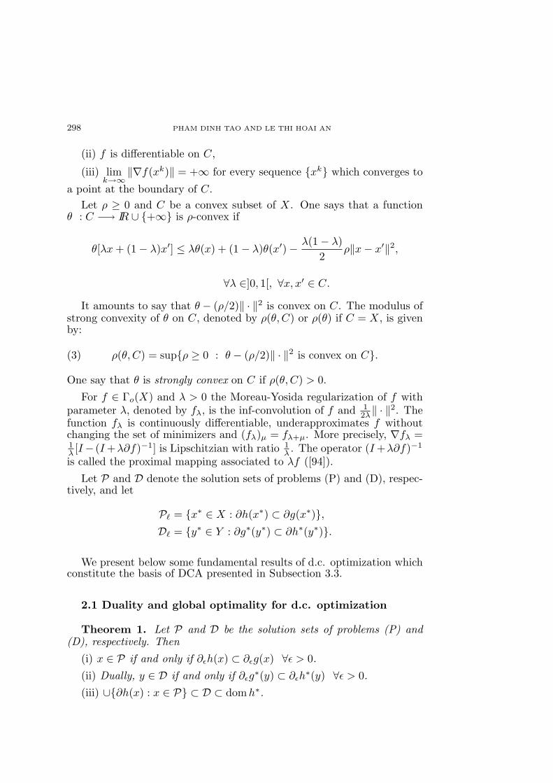
(ii) f is differentiable on C,
(iii) limk→∞
‖∇f(xk)‖ = +∞ for every sequence xk which converges to
a point at the boundary of C.Let ρ ≥ 0 and C be a convex subset of X. One says that a function
θ : C −→ IR ∪ +∞ is ρ-convex if
θ[λx + (1− λ)x′] ≤ λθ(x) + (1− λ)θ(x′)− λ(1− λ)2
ρ‖x− x′‖2,
∀λ ∈]0, 1[, ∀x, x′ ∈ C.
It amounts to say that θ − (ρ/2)‖ · ‖2 is convex on C. The modulus ofstrong convexity of θ on C, denoted by ρ(θ, C) or ρ(θ) if C = X, is givenby:
(3) ρ(θ, C) = supρ ≥ 0 : θ − (ρ/2)‖ · ‖2 is convex on C.
One say that θ is strongly convex on C if ρ(θ, C) > 0.
For f ∈ Γo(X) and λ > 0 the Moreau-Yosida regularization of f withparameter λ, denoted by fλ, is the inf-convolution of f and 1
2λ‖ · ‖2. Thefunction fλ is continuously differentiable, underapproximates f withoutchanging the set of minimizers and (fλ)µ = fλ+µ. More precisely, ∇fλ =1λ [I− (I +λ∂f)−1] is Lipschitzian with ratio 1
λ . The operator (I +λ∂f)−1
is called the proximal mapping associated to λf ([94]).
Let P and D denote the solution sets of problems (P) and (D), respec-tively, and let
P` = x∗ ∈ X : ∂h(x∗) ⊂ ∂g(x∗),D` = y∗ ∈ Y : ∂g∗(y∗) ⊂ ∂h∗(y∗).
We present below some fundamental results of d.c. optimization whichconstitute the basis of DCA presented in Subsection 3.3.
2.1 Duality and global optimality for d.c. optimization
Theorem 1. Let P and D be the solution sets of problems (P) and(D), respectively. Then
(i) x ∈ P if and only if ∂εh(x) ⊂ ∂εg(x) ∀ε > 0.
(ii) Dually, y ∈ D if and only if ∂εg∗(y) ⊂ ∂εh
∗(y) ∀ε > 0.
(iii) ∪∂h(x) : x ∈ P ⊂ D ⊂ domh∗.

D. C. PROGRAMMING 299
The first inclusion becomes equality if g∗ is subdifferentiable in D (inparticular if D ⊂ ri (dom g∗) or if g∗ is subdifferentiable in domh∗).
In this case D ⊂ (dom ∂g∗ ∩ dom ∂h∗).
(iv) ∪∂g∗(y) : y ∈ D ⊂ P ⊂ dom g.
The first inclusion becomes equality if h is subdifferentiable in P (inparticular if P ⊂ ri (dom h) or if h is subdifferentiable in dom g). In thiscase P ⊂ (dom ∂g ∩ dom ∂h).
The relationship between primal and dual solutions: ∪∂h(x) : x ∈P ⊂ D and ∪∂g∗(y) : y ∈ D ⊂ P is due to J.F. Toland ([108])
in the general context of duality principle dealing with linear vectorspaces in separating duality. A direct proof of the results (except forProperties (i) and (ii)) of Theorem 1, based on the theory of subdifferentialfor convex functions is given in [1], [76], [80]. The properties (i) and(ii) have been first established by J.B. Hiriart-Urruty ([37]). His proof(based on his earlier work concerning the behaviour of the ε-directionalderivative of a convex function as a function of the parameters ε) is rathercomplicated. The following proof of these properties is very simple andwell suited to our d.c. duality framework ([1], [76], [80]). In fact, they arenothing but a geometrical translation of the equality of the optimal valuein the primal and dual d.c. programs (P) and (D).Indeed, in virtue of the d.c. duality, x∗ ∈ P if and only if x∗ ∈ dom g and
(4) g(x∗)− h(x∗) ≤ h∗(y)− g∗(y), ∀y ∈ domh∗,
i.e.,
(5) g(x∗) + g∗(y) ≤ h(x∗) + h∗(y), ∀y ∈ domh∗.
On the other hand, for x∗ ∈ dom h, the property ∂εh(x∗) ⊂ ∂εg(x∗) ∀ε > 0is, by definition, equivalent to
(6) ∀ε > 0, 〈x∗, y〉+ ε ≥ h(x∗) + h∗(y) ⇒ 〈x∗, y〉+ ε ≥ g(x∗) + g∗(y).
It is easy to see the equivalence between (5) and (6), and property (i) thusis proved.
The global optimality condition in (i) is difficult to use for derivingsolution methods to problem (P). The algorithms DCA which will bedescribed in Subsection 3.1. are based on local optimality conditions.The relations (ii) and (iv) indicate that solving the primal d.c. program(P) implies solving the dual d.c. program (D) and vice-versa. It may beuseful if one of them is easier to solve than the other.
300 PHAM DINH TAO AND LE THI HOAI AN
2.2. Duality and local optimality conditions for d.c. optimization
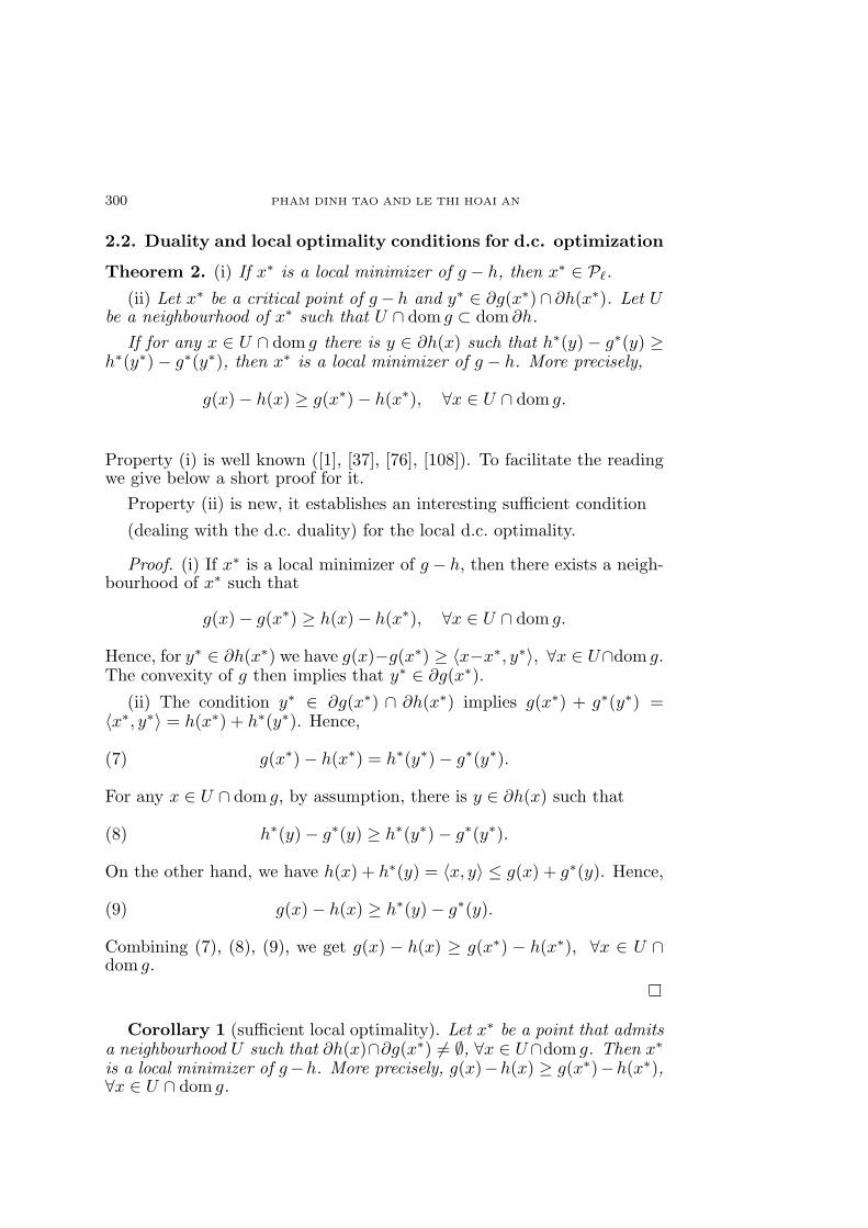
Theorem 2. (i) If x∗ is a local minimizer of g − h, then x∗ ∈ P`.
(ii) Let x∗ be a critical point of g− h and y∗ ∈ ∂g(x∗)∩ ∂h(x∗). Let Ube a neighbourhood of x∗ such that U ∩ dom g ⊂ dom ∂h.
If for any x ∈ U ∩ dom g there is y ∈ ∂h(x) such that h∗(y)− g∗(y) ≥h∗(y∗)− g∗(y∗), then x∗ is a local minimizer of g − h. More precisely,
g(x)− h(x) ≥ g(x∗)− h(x∗), ∀x ∈ U ∩ dom g.
Property (i) is well known ([1], [37], [76], [108]). To facilitate the readingwe give below a short proof for it.
Property (ii) is new, it establishes an interesting sufficient condition
(dealing with the d.c. duality) for the local d.c. optimality.
Proof. (i) If x∗ is a local minimizer of g − h, then there exists a neigh-bourhood of x∗ such that
g(x)− g(x∗) ≥ h(x)− h(x∗), ∀x ∈ U ∩ dom g.
Hence, for y∗ ∈ ∂h(x∗) we have g(x)−g(x∗) ≥ 〈x−x∗, y∗〉, ∀x ∈ U∩dom g.The convexity of g then implies that y∗ ∈ ∂g(x∗).
(ii) The condition y∗ ∈ ∂g(x∗) ∩ ∂h(x∗) implies g(x∗) + g∗(y∗) =〈x∗, y∗〉 = h(x∗) + h∗(y∗). Hence,
(7) g(x∗)− h(x∗) = h∗(y∗)− g∗(y∗).
For any x ∈ U ∩ dom g, by assumption, there is y ∈ ∂h(x) such that
(8) h∗(y)− g∗(y) ≥ h∗(y∗)− g∗(y∗).
On the other hand, we have h(x) + h∗(y) = 〈x, y〉 ≤ g(x) + g∗(y). Hence,
(9) g(x)− h(x) ≥ h∗(y)− g∗(y).
Combining (7), (8), (9), we get g(x) − h(x) ≥ g(x∗) − h(x∗), ∀x ∈ U ∩dom g.
Corollary 1 (sufficient local optimality). Let x∗ be a point that admitsa neighbourhood U such that ∂h(x)∩∂g(x∗) 6= ∅, ∀x ∈ U∩dom g. Then x∗is a local minimizer of g−h. More precisely, g(x)−h(x) ≥ g(x∗)−h(x∗),∀x ∈ U ∩ dom g.
D. C. PROGRAMMING 301
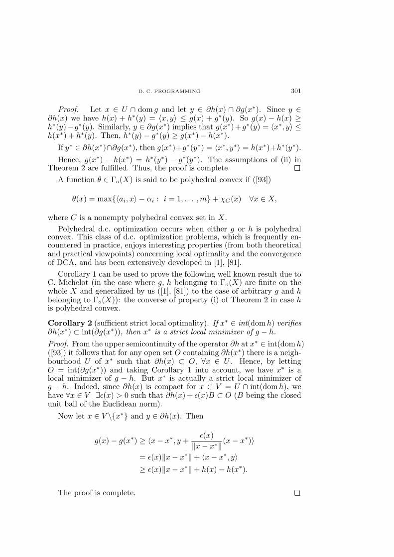
Proof. Let x ∈ U ∩ dom g and let y ∈ ∂h(x) ∩ ∂g(x∗). Since y ∈∂h(x) we have h(x) + h∗(y) = 〈x, y〉 ≤ g(x) + g∗(y). So g(x) − h(x) ≥h∗(y)−g∗(y). Similarly, y ∈ ∂g(x∗) implies that g(x∗)+g∗(y) = 〈x∗, y〉 ≤h(x∗) + h∗(y). Then, h∗(y)− g∗(y) ≥ g(x∗)− h(x∗).
If y∗ ∈ ∂h(x∗)∩∂g(x∗), then g(x∗)+g∗(y∗) = 〈x∗, y∗〉 = h(x∗)+h∗(y∗).
Hence, g(x∗) − h(x∗) = h∗(y∗) − g∗(y∗). The assumptions of (ii) inTheorem 2 are fulfilled. Thus, the proof is complete.
A function θ ∈ Γo(X) is said to be polyhedral convex if ([93])
θ(x) = max〈ai, x〉 − αi : i = 1, . . . , m+ χC(x) ∀x ∈ X,
where C is a nonempty polyhedral convex set in X.Polyhedral d.c. optimization occurs when either g or h is polyhedral
convex. This class of d.c. optimization problems, which is frequently en-countered in practice, enjoys interesting properties (from both theoreticaland practical viewpoints) concerning local optimality and the convergenceof DCA, and has been extensively developed in [1], [81].
Corollary 1 can be used to prove the following well known result due toC. Michelot (in the case where g, h belonging to Γo(X) are finite on thewhole X and generalized by us ([1], [81]) to the case of arbitrary g and hbelonging to Γo(X)): the converse of property (i) of Theorem 2 in case his polyhedral convex.
Corollary 2 (sufficient strict local optimality). If x∗ ∈ int(dom h) verifies∂h(x∗) ⊂ int(∂g(x∗)), then x∗ is a strict local minimizer of g − h.
Proof. From the upper semicontinuity of the operator ∂h at x∗ ∈ int(domh)([93]) it follows that for any open set O containing ∂h(x∗) there is a neigh-bourhood U of x∗ such that ∂h(x) ⊂ O, ∀x ∈ U . Hence, by lettingO = int(∂g(x∗)) and taking Corollary 1 into account, we have x∗ is alocal minimizer of g − h. But x∗ is actually a strict local minimizer ofg − h. Indeed, since ∂h(x) is compact for x ∈ V = U ∩ int(domh), wehave ∀x ∈ V ∃ε(x) > 0 such that ∂h(x) + ε(x)B ⊂ O (B being the closedunit ball of the Euclidean norm).
Now let x ∈ V \x∗ and y ∈ ∂h(x). Then
g(x)− g(x∗) ≥ 〈x− x∗, y +ε(x)
‖x− x∗‖ (x− x∗)〉= ε(x)‖x− x∗‖+ 〈x− x∗, y〉≥ ε(x)‖x− x∗‖+ h(x)− h(x∗).
The proof is complete.
302 PHAM DINH TAO AND LE THI HOAI AN
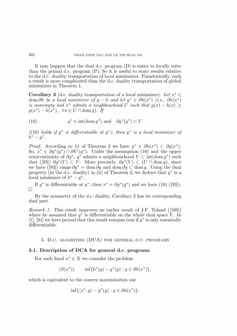
It may happen that the dual d.c. program (D) is easier to locally solvethan the primal d.c. program (P). So it is useful to state results relativeto the d.c. duality transportation of local minimizers. Paradoxically, sucha result is more complicated than the d.c. duality transportation of globalminimizers in Theorem 1.
Corollary 3 (d.c. duality transportation of a local minimizer). Let x∗ ∈dom ∂h be a local minimizer of g − h and let y∗ ∈ ∂h(x∗) (i.e., ∂h(x∗)is nonempty and x∗ admits a neighbourhood U such that g(x) − h(x) ≥g(x∗)− h(x∗), ∀x ∈ U ∩ dom g). If
(10) y∗ ∈ int(dom g∗) and ∂g∗(y∗) ⊂ U
((10) holds if g∗ is differentiable at y∗), then y∗ is a local minimizer ofh∗ − g∗.
Proof. According to (i) of Theorem 2 we have y∗ ∈ ∂h(x∗) ⊂ ∂g(x∗).So, x∗ ∈ ∂g∗(y∗) ∩ ∂h∗(y∗). Under the assumption (10) and the uppersemicontinuity of ∂g∗, y∗ admits a neighbourhood V ⊂ int(dom g∗) suchthat ([93]) ∂g∗(V ) ⊂ U . More precisely, ∂g∗(V ) ⊂ (U ∩ dom g), sincewe have ([93]) range ∂g∗ = dom ∂g and dom ∂g ⊂ dom g. Using the dualproperty (in the d.c. duality) in (ii) of Theorem 2, we deduce that y∗ is alocal minimizer of h∗ − g∗.
If g∗ is differentiable at y∗, then x∗ = ∂g∗(y∗) and we have (10) ([93]).
By the symmetry of the d.c. duality, Corollary 3 has its correspondingdual part.
Remark 1. This result improves an earlier result of J.F. Toland ([108])where he assumed that g∗ is differentiable on the whole dual space Y . In[1], [81] we have proved that this result remains true if g∗ is only essentiallydifferentiable.
3. D.c. algorithm (DCA) for general d.c. programs
3.1. Description of DCA for general d.c. programs
For each fixed x∗ ∈ X we consider the problem
(S(x∗)) infh∗(y)− g∗(y) : y ∈ ∂h(x∗),
which is equivalent to the convex maximization one
inf〈x∗, y〉 − g∗(y) : y ∈ ∂h(x∗).
D. C. PROGRAMMING 303
Similarly, for each fixed y∗ ∈ Y , for duality, we define the problem
(T (y∗)) infg(x)− h(x) : x ∈ ∂g∗(y∗).This problem is equivalent to
inf〈x, y∗〉 − h(x) : x ∈ ∂g∗(y∗).Let S(x∗), T (y∗) denote the solution sets of Problems (S(x∗)) and (T (y∗)),respectively.
The complete form of DCA is based upon duality of d.c. optimizationdefined by (P) and (D). It allows approximating a point (x∗, y∗) ∈ P`×D`.From a point xo ∈ dom g given in advance, the algorithm consists ofconstructing two sequences xk and yk defined by
(11) yk ∈ S(xk); xk+1 ∈ T (yk).
The complete DCA can be viewed as a sort of decomposition approachof the primal and dual problems (P), (D). From a practical point of view,although the problems (S(xk)) and (T (xk)) are simpler than (P), (D)(we work in ∂h(xk) and ∂g∗(yk) with convex maximization problems),they remain nonconvex programs and thus are still of a difficult task (seeSubsection 3.3). In practice the following simplified form of DCA is used:
• Simplified form of DCA:
The idea of the simplified DCA is to construct two sequences xk andyk (candidates to primal and dual solutions) which are easy to calculateand satisfy the following conditions:
(i) The sequences (g − h)(xk) and (h∗ − g∗)(yk) are decreasing.
(ii) Every limit point x∗ (resp. y∗) of the sequence xk (resp. yk)is a critical point of g − h (resp. h∗ − g∗).
These conditions suggest constructing two sequences xk and yk,starting from a given point xo ∈ dom g by setting
yk ∈ ∂h(xk); xk+1 ∈ ∂g∗(yk).
Interpretation of the simplified DCA:

304 PHAM DINH TAO AND LE THI HOAI AN
At each iteration k we do the following:
xk ∈ ∂g∗(yk−1) → yk ∈ ∂h(xk)
= argminh∗(y)− [g∗(yk−1) + 〈xk, y − yk−1〉] : y ∈ Y , (Dk)
yk ∈ ∂h(xk) → xk+1 ∈ ∂g∗(yk)
= argming(x)− [h(xk) + 〈x− xk, yk〉] : x ∈ X. (Pk)
Problem (Pk) is a convex program obtained from (P) by replacing h withits affine minorization defined by yk ∈ ∂h(xk). Similarly, the convexproblem (Dk) is obtained from (D) by using the affine minorization ofg∗ defined by xk ∈ ∂g∗(yk−1). Here we can see the complete symmetrybetween problems (Pk) and (Dk), and between the sequences xk andyk relative to the duality of d.c. optimization. The two forms of DCAare identical if g∗ and h are essentially differentiable.
• Well definiteness of DCA:
DCA is well defined if one can construct two sequences xk and ykas above from an arbitrary initial point xo ∈ dom g. We have xk+1 ∈∂g∗(yk) and yk ∈ ∂h(xk), ∀k ≥ 0. So xk ⊂ range ∂g∗ = dom ∂g andyk ⊂ range ∂h = dom ∂h∗. Then it is clear that
Lemma 1. Sequences xk, yk in DCA are well defined if and only if
dom ∂g ⊂ dom ∂h and dom ∂h∗ ⊂ dom ∂g∗.
Since for ϕ ∈ Γo(X) we have ri(dom ϕ) ⊂ dom ∂ϕ ⊂ domϕ ([93])(ri (dom ϕ) stands for the relative interior of domϕ) we can say, underthe essential assumption (1), that DCA is in general well defined.
Remark 2. A d.c. function f has infinitely many d.c. decompositions. Forexample if f = g−h, then f = (g+θ)−(h+θ) for every θ ∈ Γo(X) finite onthe whole X. It is clear that the primal d.c. programs (P) corresponding tothe two d.c. decompositions of the objective function f are identical. Buttheir dual programs are quite different and so is DCA relative to these d.c.decompositions. In other words, there are as many DCA as there are d.c.decompositions of the objective function f . It is so useful to find a suitabled.c. decomposition of f since it may have an important influence on theefficiency of DCA for its solution. This question is intimately related tothe regularization techniques in d.c. programming ([1], [76], [80]).

D. C. PROGRAMMING 305
3.2. Convergence of DCA for general d.c. programs
Let ρi and ρ∗i , (i = 1, 2) be real nonnegative numbers such that 0 ≤ρi < ρ(fi) (resp. 0 ≤ ρ∗i < ρ(f∗i )) where ρi = 0 (resp. ρ∗i = 0) if ρ(fi) = 0(resp. ρ(f∗i ) = 0) and ρi (resp. ρ∗i ) may take the value ρ(fi) (resp. ρ(f∗i ))if it is attained. We next set f1 = g and f2 = h. Also let dxk := xk+1−xk
and dyk := yk+1 − yk.
The basic convergence theorem of DCA for general d.c. programmingwill be stated below.
Theorem 3. Suppose that the sequences xk and yk are defined bythe simplified DCA. Then we have
(i) (g − h)(xk+1) ≤ (h∗ − g∗)(yk)−maxρ2
2‖dxk‖2, ρ∗2
2‖dyk‖2
≤ (g − h)(xk)−maxρ1 + ρ2
2‖dxk‖2, ρ∗1
2‖dyk−1‖2
+ρ2
2‖dxk‖2, ρ∗1
2‖dyk−1‖2 +
ρ∗22‖dyk‖2
.
The equality (g − h)(xk+1) = (g − h)(xk) holds if and only if xk ∈∂g∗(yk), yk ∈ ∂h(xk+1) and (ρ1 + ρ2)dxk = ρ∗1dyk−1 = ρ∗2dyk = 0. In thiscase
• (g − h)(xk+1) = (h∗ − g∗)(yk) and xk, xk+1 are the critical points ofg−h satisfying yk ∈ (∂g(xk)∩∂h(xk)) and yk ∈ (∂g(xk+1)∩∂h(xk+1)),
• yk is a critical point of h∗ − g∗ satisfying [xk, xk+1] ⊂ ((∂g∗(yk) ∩∂h∗(yk)),
• xk+1 = xk if ρ(g) + ρ(h) > 0, yk = yk−1 if ρ(g∗) > 0 and yk = yk+1 ifρ(h∗) > 0.
(ii) Similarly, for the dual problem we have
(h∗ − g∗)(yk+1) ≤ (g − h)(xk+1)−maxρ1
2‖dxk+1‖2, ρ∗1
2‖dyk‖2
≤ (h∗ − g∗)(yk)−maxρ1
2‖dxk+1‖2 +
ρ2
2‖dxk‖2,
ρ∗12‖dyk‖2 +
ρ2
2‖dxk‖2, ρ∗1 + ρ∗2
2‖dyk‖2
.
The equality (h∗−g∗)(yk+1) = (h∗−g∗)(yk) holds if and only if xk+1 ∈∂g∗(yk+1), yk ∈ ∂h(xk+1) and (ρ∗1 + ρ∗2)dyk = ρ2dxk = ρ1dxk+1 = 0. Inthis case
306 PHAM DINH TAO AND LE THI HOAI AN
• (h∗ − g∗)(yk+1) = (g − h)(xk+1) and yk, yk+1 are the critical points ofh∗− g∗ satisfying xk+1 ∈ (∂g∗(yk)∩∂h∗(yk)) and xk+1 ∈ (∂g∗(yk+1)∩∂h∗(yk+1)),
• xk+1 is a critical point of g − h satisfying [yk, yk+1] ⊂ ((∂g(xk+1) ∩∂h(xk+1)),
• yk+1 = yk if ρ(g∗)+ρ(h∗) > 0, xk+1 = xk if ρ(h) > 0 and xk+1 = xk+2
if ρ(g) > 0.
(iii) If α is finite then the decreasing sequences (g−h)(xk) and (h∗−g∗)(yk) converge to the same limit β ≥ α, i.e., lim
k→+∞(g − h)(xk) =
limk→+∞
(h∗ − g∗)(yk) = β. If ρ(g) + ρ(h) > 0 (resp. ρ(g∗) + ρ(h∗) > 0),
then limk→+∞
xk+1 − xk = 0 (resp. limk→+∞
yk+1 − yk = 0).
Moreover, limk→+∞
g(xk) + g∗(yk) − 〈xk, yk〉 = 0 = limk→+∞
h(xk+1) +
h∗(yk)− 〈xk+1, yk〉.(iv) If α is finite and the sequences xk and yk are bounded, then
for every limit x∗ of xk (resp. y∗ of yk) there exists a cluster pointy∗ of yk (resp. x∗ of xk) such that
• (x∗, y∗) ∈ [∂g∗(y∗) ∩ ∂h∗(y∗)] × [∂g(x∗) ∩ ∂h(x∗)] and (g − h)(x∗) =(h∗ − g∗)(y∗) = β,
• limk→+∞
g(xk) + g∗(yk) = limk→+∞
〈xk, yk〉.
Proof. First, we need the following results
Proposition 2. Suppose that the sequences xk and yk are generatedby the simplified DCA. Then we have
(i) (g−h)(xk+1) ≤ (h∗−g∗)(yk)−ρ22 ‖dxk‖2 ≤ (g−h)(xk)−ρ1+ρ2
2 ‖dxk‖2.The equality (g − h)(xk+1) = (g − h)(xk) holds if and only if
xk ∈ ∂g∗(yk), yk ∈ ∂h(xk+1) and (ρ1 + ρ2)‖dxk‖ = 0.
(ii) Similarly, by duality, we have
(h∗ − g∗)(yk+1) ≤ (g − h)(xk+1)− ρ∗12‖dyk‖2
≤ (h∗ − g∗)(yk)− ρ∗1 + ρ∗22
‖dyk‖2.

D. C. PROGRAMMING 307
The equality (h∗ − g∗)(yk+1) = (h∗ − g∗)(yk) holds if and only if
xk+1 ∈ ∂g∗(yk+1), yk ∈ ∂h(xk+1) and (ρ∗1 + ρ∗2)‖dyk‖ = 0.
Proof of Proposition 2. (i) The inclusion yk ∈ ∂h(xk) follows that
h(xk+1) ≥ h(xk) + 〈xk+1 − xk, yk〉+ρ2
2‖dxk‖2. Hence,
(12) (g − h)(xk+1) ≤ g(xk+1)− 〈xk+1 − xk, yk〉 − h(xk)− ρ2
2‖dxk‖2.
Likewise, xk+1 ∈ ∂g∗(yk) implies
g(xk) ≥ g(xk+1) + 〈xk − xk+1, yk〉+ρ1
2‖dxk‖2.
So,
(13) g(xk+1)− 〈xk+1 − xk, yk〉 − h(xk) ≤ (g − h)(xk)− ρ1
2‖dxk‖2.
On the other hand,
xk+1 ∈ ∂g∗(yk) ⇔ 〈xk+1, yk〉 = g(xk+1) + g∗(yk),(14)
yk ∈ ∂h(xk) ⇔ 〈xk, yk〉 = h(xk) + h∗(yk).(15)
Thus,
(16) g(xk+1)− 〈xk+1 − xk, yk〉 − h(xk) = h∗(yk)− g∗(yk).
Finally, combining (12), (13) and (16), we get(17)
(g−h)(xk+1) ≤ (h∗− g∗)(yk)− ρ2
2‖dxk‖2 ≤ (g−h)(xk)− ρ1 + ρ2
2‖dxk‖2.
If ρ1 +ρ2 > 0, the last statement of (i) is an immediate consequence of theequality dxk = 0 and the construction of the sequences xk and yk.
It is clear that there exist ρ1 and ρ2 such that ρ1 +ρ2 > 0 if and only ifρ(h) + ρ(g) > 0. In the case ρ(h) = ρ(g) = 0, (15) implies the equivalencebetween (g − h)(xk+1) = (g − h)(xk) and the combination (18) and (19):
(g − h)(xk+1) = (h∗ − g∗)(yk),(18)
(h∗ − g∗)(yk) = (g − h)(xk).(19)

308 PHAM DINH TAO AND LE THI HOAI AN
We then deduce from (14) and (18) that h(xk+1) + h∗(yk) = 〈xk+1, yk〉,i.e., yk ∈ ∂h(xk+1).
Similarly, (15) and (19) give g(xk) + g∗(yk) = 〈xk, yk〉, i.e., xk ∈∂g∗(yk).
Property (ii) is analogously proved.
The following result is an important consequence of Proposition 2
Corollary 4.
(i) (g − h)(xk+1) ≤ (h∗ − g∗)(yk)− ρ2
2‖dxk‖2
≤ (g − h)(xk)−[ρ∗1
2‖dyk−1‖2 +
ρ2
2‖dxk‖2
].
(ii) (g − h)(xk+1) ≤ (h∗ − g∗)(yk)− ρ∗22‖dyk‖2
≤ (g − h)(xk)−[ρ∗1
2‖dyk−1‖2 +
ρ∗22‖dyk‖2
].
The equality (g − h)(xk+1) = (g − h)(xk) holds if and only if
xk ∈ ∂g∗(yk), yk ∈ ∂h(xk+1) and (ρ1 + ρ2)dxk = ρ∗1dyk−1 = ρ∗2dyk = 0.
Similarly, by duality, we have
iii) (h∗ − g∗)(yk+1) ≤ (g − h)(xk+1)ρ∗12‖dyk‖2
≤ (h∗ − g∗)(yk)−[ρ∗1
2‖dyk‖2 +
ρ2
2‖dxk‖2
].
(iv) (h∗ − g∗)(yk+1) ≤ (g − h)(xk+1)− ρ1
2‖dxk+1‖2
≤ (h∗ − g∗)(yk)−[ρ1
2‖dxk+1‖2 +
ρ2
2‖dxk‖2
].
The equality (h∗ − g∗)(yk+1) = (h∗ − g∗)(yk) holds if and only if
xk+1 ∈ ∂g∗(yk+1), yk ∈ ∂h(xk+1) and
(ρ∗1 + ρ∗2)dyk = ρ2dxk = ρ1dxk+1 = 0.
Proof. The inequalities in (i) and (ii) are easily deduced from Properties(i) and (ii) of Proposition 2. The inequalities in (iii) and (iv) can be shown
D. C. PROGRAMMING 309
by the same arguments as in the proof of Proposition 2.
We are now in a position to demonstrate Theorem 3.
Proof of Theorem 3. Properties (i) and (ii) are proved analogously, there-fore we give here the proof for (i) only.
The first inequality of (i) is an immediate consequence of (i) and (ii) ofCorollary 4.
• If ρ2‖dxk‖2 ≤ ρ∗2‖dyk‖2, then (ii) of Corollary 4 follows that
(h∗ − g∗)(yk)−maxρ2
2‖dxk‖2, ρ∗2
2‖dyk‖2
= (h∗ − g∗)(yk)− ρ∗2
2‖dyk‖2
≤ (g − h)(xk)−ρ∗1
2‖dyk−1‖2 +
ρ∗22‖dyk‖2
.
Parallelly, Property (i) of Corollary 4 implies
(h∗ − g∗)(yk)− ρ∗22‖dyk‖2 ≤ (h∗ − g∗)(yk)− ρ2
2‖dxk‖2
≤ (g − h)(xk)−[ρ∗1
2‖dyk−1‖2 +
ρ2
2‖dxk‖2
].
On the other hand, by (i) of Proposition 2
(h∗ − g∗)(yk)− ρ∗22‖dyk‖2 ≤ (h∗ − g∗)(yk)− ρ2
2‖dxk‖2
≤ (g − h)(xk)− ρ1 + ρ2
2‖dxk‖2.
Combining these inequalities, we get the second inequality of (i).
• If ρ∗2‖dyk‖2 ≤ ρ2‖dxk‖2, then by using the same arguments we caneasily show the second inequality of (i). The first property of (iii) isevident. We will prove the last one. Taking (16) and (i) into account,we have
limk→+∞
(g − h)(xk+1) = limk→+∞
g(xk+1)− 〈xk+1 − xk, yk〉 − h(xk)
= limk→+∞
(g − h)(xk).
The second equality implies limk→+∞
g(xk+1)−〈xk+1−xk, yk〉−g(xk) =
0, i.e., limk→+∞
g(xk) + g∗(yk)− 〈xk, yk〉 = 0, since xk+1 ∈ ∂g∗(yk).

310 PHAM DINH TAO AND LE THI HOAI AN
Likewise, it results from the first equality that limk→+∞
h(xk+1)− 〈xk+1 −xk, yk〉 − h(xk) = 0, i.e., lim
k→+∞h(xk+1) + h∗(yk)− 〈xk+1, yk〉 = 0 since
yk ∈ ∂h(yk).
(iv) We assume α is finite and the sequences xk and yk are boun-ded. Let x∗ be a limit point of xk. For the sake of simplicity wewrite lim
k→+∞xk = x∗. We can suppose (by extracting a subsequence if
necessary) that the sequence yk converges to y∗ ∈ ∂h(x∗). Property(iii) then implies
limk→+∞
g(xk) + g∗(yk) = limk→+∞
〈xk, yk〉 = 〈x∗, y∗〉.
Let θ(x, y) = g(x) + g∗(y) for (x, y) ∈ X × Y . It is clear that θ ∈Γo(X × Y ). Then the lower semicontinuity of θ implies
θ(x∗, y∗) ≤ limk→+∞
inf θ(xk, yk) = limk→+∞
θ〈xk, yk〉 = 〈x∗, y∗〉,
i.e., θ(x∗, y∗) = g(x∗) + g∗(y∗) = 〈x∗, y∗〉. In other words, y∗ ∈ ∂g(x∗).According to Lemma 2 stated below we have
limk→+∞
h(xk) = h(x∗) and limk→+∞
h∗(yk) = h∗(y∗),
since yk ∈ ∂h(xk), xk → x∗ and yk → y∗.
Hence, in virtue of (iii),
limk→+∞
(g − h)(xk) = limk→+∞
g(xk)− limk→+∞
h(xk)
= limk→+∞
g(xk)− h(x∗) = β,
limk→+∞
(h∗ − g∗)(yk) = limk→+∞
h∗(yk)− limk→+∞
g∗(yk)
= h∗(y∗)− limk→+∞
g∗(yk) = β.
It then suffices to show that
limk→+∞
g(xk) = g(x∗); limk→+∞
g∗(yk) = g∗(y∗).
D. C. PROGRAMMING 311
Since limk→+∞
g(xk) and limk→+∞
g∗(yk) exist, (iii) implies
g(x∗) + g∗(y∗) = limk→+∞
g(xk) + g∗(yk) = limk→+∞
g(xk) + limk→+∞
g∗(yk).
Further, because of the lower semicontinuity of g and g∗,
limk→+∞
g(xk) = limk→+∞
inf g(xk) ≥ g(x∗),
limk→+∞
g∗(yk) = limk→+∞
inf g∗(yk) ≥ g∗(y∗).
The former equalities imply that these last inequalities are in fact equali-ties. The proof of Theorem 3 is complete.
Lemma 2. Let h ∈ Γo(X) and xk be a sequence of elements in X suchthat
(i) xk → x∗,
(ii) There exists a bounded sequence yk with yk ∈ ∂h(xk),
(iii) ∂h(x∗) is nonempty.
Then limk→+∞
h(xk) = h(x∗).
Proof. Indeed, let y∗ ∈ ∂h(x∗). Then h(xk) ≥ h(x∗) + 〈xk − x∗, y∗〉, ∀k.Since yk ∈ ∂h(xk), we have h(x∗) ≥ h(xk) + 〈x∗ − xk, yk〉, ∀k. Hence,h(xk) ≤ h(x∗) + 〈xk − x∗, yk〉, ∀k. As xk → x∗, we have lim
k→+∞〈xk −
x∗, y∗〉 = 0. Moreover, limk→+∞
〈xk − x∗, yk〉 = 0, since the sequence yk is
bounded. Consequently, limk→+∞
h(xk) = h(x∗).
Comments on Theorem 3.
(i) Properties (i) and (ii) prove that DCA is a descent method for bothprimal and dual programs. DCA provides critical points for (P) and (D)after finitely many operations if there is no strict decrease of the primal(or dual) objective function.
(ii) If C and D are convex sets such that xk ⊂ C and yk ⊂ D,then Theorem 3 remains valid if we replace ρ(fi) by ρ(fi, C) and ρ(f∗i )by ρ(f∗i , D) for i = 1, 2. By this way we may improve the results in thetheorem.
(iii) In (ii) of Theorem 3, the convergence of the whole sequence xk(resp. yk) can be ensured under the following conditions ([65], [71]):

312 PHAM DINH TAO AND LE THI HOAI AN
• xk is bounded;
• The set of limit points of xk is finite;
• limk→+∞
‖xk+1 − xk‖ = 0.
(iv) In general, the qualities (robustness, stability, rate of convergenceand globality of sought solutions) of DCA, in both complete and simpli-fied forms, depend upon the d.c. decomposition of the function f . Theo-rem 3 shows how strong convexity of d.c. components in primal and dualproblems can influence on DCA. To make the d.c. components (of theprimal objective function f = g−h) strongly convex we usually apply thefollowing process
f = g − h =(g +
λ
2‖ · ‖2
)−
(h +
λ
2‖ · ‖2
).
In this case the d.c. components in the dual problem will be continuouslydifferentiable. Parallelly inf-convolution of g and h with λ
2 ‖ · ‖2 will makethe d.c. components (in dual problem) strongly convex and the d.c. com-ponents of the primal objective function continuously differentiable. For adetailed study of regularization techniques in d.c. optimization, see Section5 and [1], [76], [80].
3.3. How to restart simplified DCA for obtaining x∗ such that∂h(x∗) ⊂ ∂g(x∗)
As mentioned above, the complete DCA theoretically provides a x∗
such that ∂h(x∗) ⊂ ∂g(x∗). In practice, except for the cases where theconvex maximization problems (S(xk) and (T (yk)) are easy to solve, onegenerally uses the simplified DCA. It is worth noting that if the simplifiedDCA terminates at some point x∗ for which ∂h(x∗) is not contained in∂g(x∗), then one can reduce the objective function value by restarting itfrom a new initial point xo = x∗ with yo ∈ ∂h(xo) such that yo 6∈ ∂g(xo).In fact, since
g(x1) + g∗(yo) = 〈x1, yo〉 ≤ h(x1)− h(xo) + 〈xo, yo〉,and 〈xo, yo〉 < g(xo) + g∗(yo) because yo 6∈ ∂g(xo), we have
g(x1) + g∗(yo) < h(x1)− h(xo) + g(xo) + g∗(yo).
Hence,g(x1)− h(x1) < g(xo)− h(xo).

D. C. PROGRAMMING 313
4. Polyhedral d.c. optimization problems and finite
convergence of DCA with fixed choices of subgradients
4.1. Polyhedral d.c. program
We suppose that in Problem (P) either g or h is polyhedral convex.We may assume that h is a polyhedral convex function given by h(x) =max〈ai, x〉 − αi : i = 1, . . . , m + χC(x), where χC is the indicatorfunction of a nonempty polyhedral convex set C in X. (If in (P ) g ispolyhedral and h is not so, then we consider the dual problem (D), sinceg∗ is polyhedral). Throughout this subsection we assume that the optimalvalue α of problem (P) is finite which implies that dom g ⊂ domh = C.Thus, (P) is equivalent to the problem
(P ) α = infg(x)− h(x) : x ∈ X,
where h(x) = max〈ai, x〉 − αi : i ∈ I with I = 1, . . . , m. By this waywe can avoid +∞−(+∞) in (P). Clearly, α = inf
i∈Iinf
x∈Xg(x)−(〈ai, x〉−αi).
For each i ∈ I, let
(Pi) βi = infg(x)− (〈ai, x〉 − αi) : x ∈ X
whose solution set is ∂g∗(ai).
The dual problem (D) of (P ) is:
(D) α = infh∗(y)− g∗(y) : y ∈ co ai : i ∈ I,
where α verifies α = infh∗(y)− g∗(y) : y ∈ ai : i ∈ I.Also, let J(α) = i ∈ I : βi = α and I(x) = i ∈ I : 〈ai, x〉 − αi =
h(x). We have the following result ([1], [2], [81]).
Theorem 4. (i) x∗ ∈ P if and only if I(x∗) ⊂ J(α) and x∗ ∈ ∩∂g∗(ai) :i ∈ I(x∗).
(ii) P = ∪∂g∗(ai) : i ∈ J(α). If ai : i ∈ I ⊂ dom ∂g∗, then P 6= ∅.(iii) h(x) = max〈x, y〉 − h∗(y) : y ∈ coai : i ∈ I = max〈ai, x〉 −
h∗(ai) : i ∈ I.(iv) J(α) = i ∈ I : ai ∈ D and h∗(ai) = αi; D ⊃ ai : i ∈ J(α).The proof of this theorem is very technical, the interested reader is
therefore referred to [1], [2], [81] for a detailed analysis.

314 PHAM DINH TAO AND LE THI HOAI AN
4.2. Finite convergence of DCA
From 4.1 we see that (globally) solving the polyhedral d.c. optimizationproblem (P ) amounts to solving m convex programs (Pi) (i ∈ I). Forgenerating P one can first determine J(α) and then apply Theorem 4.In practice this can be effectively done if m is relatively small. In casewhen m is large we use the simplified DCA for solving (locally) Problem(P ). Recall that (Lemma 1) the simplified DCA is well defined if andonly if co ai : i ∈ I ⊂ dom ∂g∗. Because of the finiteness of α, dom g ⊂domh = C and co ai : i ∈ I ⊂ dom g∗. The simplified DCA in this caseis described as follows: Let xo be chosen in advance. Set yk ∈ ∂h(xk) =co ai : i ∈ I(xk); xk+1 ∈ ∂g∗(yk) By setting yk = ai, i ∈ I(xk) thecalculation of xk+1 is reduced to solve the convex program
(Pi) ming(x)− 〈yk, x〉 : x ∈ X.
Note that if yk = ai with i ∈ J(α), then, by Theorem 4, xk+1 ∈ P.
Now let H and G∗ be two mappings defined respectively in dom ∂h = Xand in dom ∂g∗ such that H(x) ∈ ∂h(x), ∀x ∈ X and G∗(y) ∈ ∂g∗(y)∀y ∈ dom ∂g∗. The simplified DCA with a fixed choice of subgradients isdefined as:
yk = H(xk) ; xk+1 = G∗(yk).
It is clear that for a polyhedral d.c. optimization problem range H is finiteif h is polyhedral convex, and range G∗ is finite if g is polyhedral convex.In each of these cases the sequences xk and yk are discrete (i.e., theyhave only finitely many different elements).
Theorem 5 ([1], [2], [81]). (i) The discrete sequences (g − h)(xk) and(h∗ − g∗)(yk) are decreasing and convergent.
(ii) The discrete sequences xk and yk have the same property: ei-ther they are convergent or cyclic with the same period p. In the lattercase the sequences xk and yk contain exactly p limit points that are allcritical points of g−h. Moreover, if ρ(g)+ρ(g∗) > 0, then these sequencesare convergent.
The proof of this theorem follows immediately from Theorem 3 and thediscrete character of the sequences xk and yk.4.3. Natural choice of subgradients in DCA
Let f ∈ Γo(X) and T be a selection of ∂f , i.e., Tx ∈ ∂f(x), ∀x ∈dom ∂f . T is said to be a natural choice of subgradients of f if the con-
D. C. PROGRAMMING 315
ditions Tx ∈ ri ∂f(x) and ∂f(x) = ∂f(x′) imply that Tx = Tx′. Thefollowing results are useful to the proof of the finite convergence of DCA(applied to the polyhedral d.c. optimization) with the fixed choices ofsubgradients for h and g∗, and the natural choice for at least one poly-hedral function among them. The natural choice has been successfullyused in the subgradient-methods for computing bound norms of matrices([70]-[73]) and the study of the iterative behaviour of cellular automatas([75]).
Since h(x) = max〈ai, x〉 − αi : i ∈ I, one can take H by settingH(x) =
∑i∈I(x) λiai, where λi, i ∈ I(x), satisfy:
(i) λi > 0, ∀i ∈ I(x) and∑
i∈I(x) λi = 1;
(ii) λi depends only on I(x).
Lemma 3 ([75], [81]). (i) ∂h(x) = ∂h(x′) ⇔ I(x) = I(x′).
(ii) H is a natural choice of subgradients of h if and only if it is definedas above.
Consider now DCA with a fixed choice of subgradient applied to thepolyhedral d.c. optimization problem (P ). If H is a natural choice of h,then the following result strengthens that of Theorem 5.
Theorem 6 ([1], [2], [81]). The simplified DCA with a fixed choice ofsubgradients is finite.
5. Regularization techniques in d.c. programming
We consider the d.c. problem (P) and its dual problem (D) where α isfinite. In this case, dom g ⊂ domh and dom h∗ ⊂ dom g∗. As mentionedabove, it is important to obtain various equivalent d.c. forms for the primaland dual problems. The Lagrangian duality in d.c. optimization ([1], [78],[82]) and regularization techniques partly answer this question.
Regularization techniques in d.c. optimization have been early intro-duced in [76] and extensively developed in our recent works [1], [80]. Be-sides three forms of regularization techniques, we present here some resultscorresponding to the computation of modulus of strong convexity. Theseresults are essential to regularization techniques applied to DCA.
First, we introduce some related results of convex analysis:
Let ϕ,ψ ∈ Γo(X), the inf-convolution of ϕ and ψ, denoted by ϕ∇ψ, isdefined by ([51], [93])
316 PHAM DINH TAO AND LE THI HOAI AN
ϕ∇ψ(x) = infϕ(x1) + ψ(x2) : x1 + x2 = x.One says that ϕ∇ψ is exact at x = x1 + x2 if ϕ∇ψ(x) = ϕ(x1) + ψ(x2).
Likewise, ϕ∇ψ is said to be exact if it is exact at every x ∈ X. Thefollowing result is useful to regularization techniques ([51], [93]):
Theorem 7. (i) ϕ∇ψ is convex and dom ϕ∇ψ = dom ϕ + dom ψ.
(ii) (ϕ∇ψ)∗ = ϕ∗ + ψ∗.
(iii) If ri (dom ϕ) ∩ ri(dom ψ) 6= ∅, then (ϕ + ψ)∗ = ϕ∗∇ψ∗ and theinf-convolution ϕ∗∇ψ∗ is exact.
(iv) ∂ϕ(x1) ∩ ∂ψ(x2) ⊂ ∂(ϕ∇ψ)(x1 + x2).
Moreover, if ∂ϕ(x1) ∩ ∂ψ(x2) 6= ∅, then the inf-convolution ϕ∇ψ isexact at x = x1 + x2. Conversely, if ϕ∇ψ is exact at x = x1 + x2, then∂(ϕ∇ψ)(x1 + x2) = ∂ϕ(x1) ∩ ∂ψ(x2).
Let ϕ ∈ Γo(X). The function ϕ is said to be strictly convex on a convexsubset C of dom f if
ϕ(λx + (1− λ)x′) < λϕ(x) + (1−λ)ϕ(x′), ∀λ ∈]0, 1[, ∀x, x′ ∈ C, x 6= x′.
Likewise, ϕ is said to be essentially strictly convex if it is strictly convexon any convex subset of dom ∂ϕ.
Theorem 8 ([93]). Let ϕ ∈ Γo(X). Then the following conditions areequivalent
(i) ∀x ∈ domϕ, ∂ϕ(x) contains at most one element.
(ii) ϕ is essentially differentiable.
In this case ∂ϕ(x) = ∇ϕ(x) if x ∈ int(domϕ) and ∂ϕ(x) is emptyotherwise.
(iii) ϕ ∈ Γo(X) is essentially differentiable if and only if ϕ∗ is essen-tially strictly convex.
(iv) Let ϕ, ψ ∈ Γo(X) be such that ϕ is essentially differentiable andri(domϕ∗) ∩ ri(domψ∗) 6= ∅. Then ϕ∇ψ is essentially differentiable.
We present now several types of regularization techniques.
5.1. Regularizing d.c. components of the dual d.c. program
Let θ ∈ Γo(X) such that

D. C. PROGRAMMING 317
(i) dom θ ⊃ dom g;
(ii) ri(dom θ) ∩ ri(dom g) 6= ∅ and ri(dom θ) ∩ ri(domh) 6= ∅.Clearly, g + θ and h + θ are also d.c. components of f . The following
problem, by (i), is equivalent to (P ):
(P+) λα = inf(λg + θ)(x)− (λh + θ)(x) : x ∈ X,
where λ is a positive number. From (ii) the dual of (P+) is formulated by(Theorem 7)
(D+) λα = inf(λg + θ)∗(y)− (λh + θ)∗(y) : y ∈ Y = inf(λh)∗∇θ∗(y)− (λg)∗∇θ∗(y) : y ∈ Y ,
which is not equivalent to (D). This regularization, with suitable choicesof θ, makes
• d.c. components in (P+) are strongly convex: if θ is strongly convex,then so are λg + θ and λh + θ, since
ρ(λg + θ) = λρ(g) + ρ(θ); ρ(λh + θ) = λρ(h) + ρ(θ),
• d.c. components in (D+) are continuously differentiable.Indeed, for example if the sets ri(dom g) ∩ ri(dom θ) and ri(domh) ∩ri(dom θ) are nonempty and if θ∗ is essentially differentiable, then ac-cording to Theorem 8, (λg)∗∇θ∗ and (λh)∗∇θ∗ are essentially differen-tiable. In particular, if θ is finite, strictly convex on the whole X,and coercive (i.e., lim
‖x‖→+∞θ(x) = +∞), then (λg)∗∇θ∗ and (λh)∗∇θ∗ are
differentiable on E (i.e., continuously differentiable on X), since thecoerciveness of θ implies that dom θ∗ = Y (the dual space of X) andits strict convexity implies the essential differentiability of θ∗ in virtueof Theorem 8.
5.2. Regularizing d.c. components in the primal d.c. program
This regularization is introduced by considering the following d.c. pro-gram
(P∇) λα = inf(λg)∇θ(x)− (λh)∇θ(x) : x ∈ X,
where λ is a positive number and θ ∈ Γo(X) for which the followingconditions hold:
318 PHAM DINH TAO AND LE THI HOAI AN
(i) ri(λdom g∗) ∩ ri(dom θ∗) 6= ∅, ri(λdomh∗) ∩ ri(dom θ∗) 6= ∅,(ii) dom θ∗ ⊃ dom (λh)∗ = λdom h∗.
In virtue of Theorem 7, one has (λg)∗(y) = λg∗(λ−1y). Thus, dom ((λg)∗)= λ(dom g∗). The condition (i) ensures that both λg∇θ and λh∇θ are inΓo(X) (Theorem 7). The dual problem of (P+) is then given as
(D∇) λα = inf(λh∇θ)∗(y)− (λg∇θ)∗(y) : y ∈ Y = inf((λh)∗ + θ∗)(y)− ((λg)∗ + θ∗)(y) : y ∈ Y
which, by (ii), is equivalent to (D). As before, suitable choices of θ allowto obtain the continuously differentiable d.c. components in (P∇) andstrongly convex d.c. components in (D∇).
5.3. Double primal-dual regularization of d.c. components
Let λ be a positive number and ϕ, θ ∈ Γo(X) such that
(i) dom g ⊂ domϕ;
(ii) ri(dom ϕ) ∩ ri(dom g) 6= ∅, ri(dom ϕ) ∩ ri(dom h) 6= ∅;(iii) λdom g∗ + dom ϕ∗ ⊂ dom θ∗.
We consider the primal problem (P+)
(P+) λα = inf(λg + ϕ)(x)− (λh + ϕ)(x) : x ∈ X,
which is equivalent to (P). We shall regularize (P+) by applying inf-convolution with θ to d.c. components:
(P+∇) inf(λg + ϕ)∇θ(x)− (λh + ϕ)∇θ(x) : x ∈ X.
Under assumptions (ii), the dual problem of (P+∇) takes the form (The-orem 7):
(D+∇) λα = inf((λh + ϕ)∗ + θ∗)(y)− ((λg + ϕ)∗ + θ∗)(y) : y ∈ Y = inf((λh)∗∇ϕ∗ + θ∗)(y)− ((λg)∗∇ϕ∗ + θ∗)(y) : y ∈ Y .
By assumption (iii) this is equivalent to the dual problem (D+) of (P+).This double regularization, with suitable choices of ϕ and θ, allows to ob-tain both strongly convex and continuously differentiable d.c. componentsin the primal and the dual problems (P+∇) and (D+∇).
D. C. PROGRAMMING 319
In practice, we usually take θ(x) = µ2 ‖x‖2, µ > 0 which is both strongly
convex and coercive. Such a regularization is called the proximal regula-rization.
Finally, the following result ([1], [80]), whose proof is omitted here,allows to compute the strong convexity modulus of regularized d.c. com-ponents which intervenes in the convergence theorem for DCA (Theorem3).
Proposition 3. If ϕ ∈ Γo(X) and λ, µ be positive numbers, then
(i) ρ ((λϕ)∗) = λ−1ρ(ϕ∗),
(ii) ∇ [(λϕ)∗]µ (x) =(I + µ−1λ∂ϕ
)−1 (µ−1x), ∀x ∈ X,
(iii) ρ(ϕ)ρ(ϕ∗) ≤ 1,
(iv)ρ(ϕ)
1 + λρ(ϕ)≤ ρ (ϕλ) ≤ 1
λ·
6. Functions which are more convex, less convex
Let f, g ∈ Γo(X). The function f is said to be more convex than g(or g is said to be less convex than f), and we write f  g (or g ≺ f) iff = g+h with h ∈ Γo(X). The binary relation f  g has been introducedby Moreau [62]. It is almost a partial ordering on Γo(X) except for thecase that f  g and g  f only imply f = g + h with h being affine on X.
Moreau proved the following interesting result
f  12‖ · ‖2 ⇔ f∗ ≺ 1
2‖ · ‖2.
In a work related to Moreau decomposition theorem, Hiriart-Urruty andPlazanet ([62]) have obtained a characterization of convex functions g, hsuch that g + h = 1
2‖ · ‖2 ([35])
g + h =12‖ · ‖2 ⇔ ∃F ∈ Γo(X) such that
g = F∇12‖ · ‖2 and h = F ∗∇
12‖ · ‖2.
An explicit formulation is given in [35] with the help of an operation on aconvex function, which bears the name of deconvolution of a function byanother one. Given ϕ and ψ in Γo(X), the deconvolution of ϕ by ψ is the
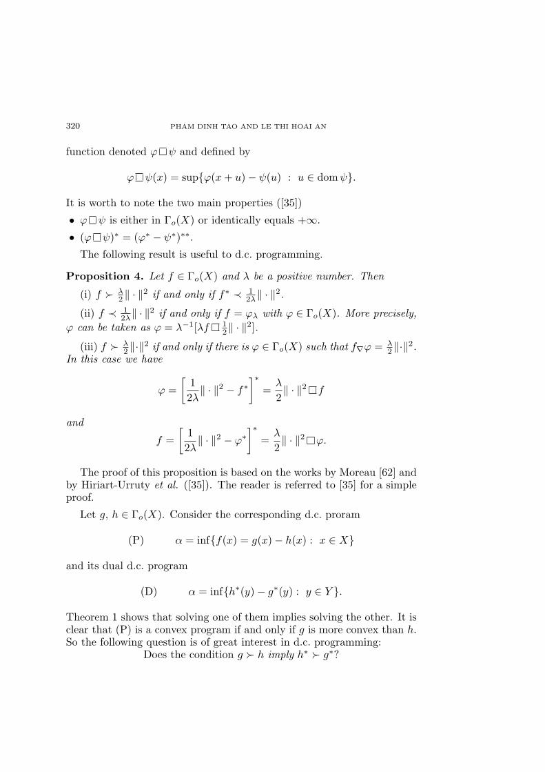
320 PHAM DINH TAO AND LE THI HOAI AN
function denoted ϕ ψ and defined by
ϕ ψ(x) = supϕ(x + u)− ψ(u) : u ∈ domψ.
It is worth to note the two main properties ([35])
• ϕ ψ is either in Γo(X) or identically equals +∞.
• (ϕ ψ)∗ = (ϕ∗ − ψ∗)∗∗.
The following result is useful to d.c. programming.
Proposition 4. Let f ∈ Γo(X) and λ be a positive number. Then
(i) f  λ2 ‖ · ‖2 if and only if f∗ ≺ 1
2λ‖ · ‖2.(ii) f ≺ 1
2λ‖ · ‖2 if and only if f = ϕλ with ϕ ∈ Γo(X). More precisely,ϕ can be taken as ϕ = λ−1[λf 1
2‖ · ‖2].(iii) f  λ
2 ‖·‖2 if and only if there is ϕ ∈ Γo(X) such that f∇ϕ = λ2 ‖·‖2.
In this case we have
ϕ =[
12λ‖ · ‖2 − f∗
]∗=
λ
2‖ · ‖2 f
and
f =[
12λ‖ · ‖2 − ϕ∗
]∗=
λ
2‖ · ‖2 ϕ.
The proof of this proposition is based on the works by Moreau [62] andby Hiriart-Urruty et al. ([35]). The reader is referred to [35] for a simpleproof.
Let g, h ∈ Γo(X). Consider the corresponding d.c. proram
(P) α = inff(x) = g(x)− h(x) : x ∈ X
and its dual d.c. program
(D) α = infh∗(y)− g∗(y) : y ∈ Y .
Theorem 1 shows that solving one of them implies solving the other. It isclear that (P) is a convex program if and only if g is more convex than h.So the following question is of great interest in d.c. programming:
Does the condition g  h imply h∗  g∗?
D. C. PROGRAMMING 321
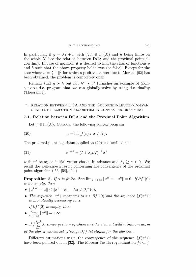
In particular, if g = λf + h with f, h ∈ Γo(X) and h being finite onthe whole X (see the relation between DCA and the proximal point al-gorithm). In case of negation it is desired to find the class of functions gand h such that the above property holds true (or false). Except for thecase where h = λ
2 ‖ · ‖2 for which a positive answer due to Moreau [62] hasbeen obtained, the problem is completely open.
Remark that g  h but not h∗  g∗ furnishes an example of (non-convex) d.c. program that we can globally solve by using d.c. duality(Theorem1).
7. Relation between DCA and the Goldstein-Levitin-Polyakgradient projection algorithm in convex programming
7.1. Relation between DCA and the Proximal Point Algorithm
Let f ∈ Γo(X). Consider the following convex program
(20) α = inff(x) : x ∈ X.
The proximal point algorithm applied to (20) is described as:
(21) xk+1 = (I + λk∂f)−1xk
with xo being an initial vector chosen in advance and λk ≥ c > 0. Werecall the well-known result concerning the convergence of the proximalpoint algorithm ([56]-[58], [94])
Proposition 5. If α is finite, then limk→+∞ ‖xk+1 − xk‖ = 0. If ∂f∗(0)is nonempty, then
• ‖xk+1 − x‖ ≤ ‖xk − x‖, ∀x ∈ ∂f∗(0),
• The sequence xk converges to x ∈ ∂f∗(0) and the sequence f(xk)is monotically decreasing to α.
If ∂f∗(0) is empty, then
• limk→+∞
‖xk‖ = +∞,
• xk/k−1∑i=1
λi converges to −v, where v is the element with minimum norm
of the closed convex set cl(range ∂f) (cl stands for the closure).
Different estimations w.r.t. the convergence of the sequence f(xk)have been pointed out in [32]. The Moreau-Yosida regularization fλ of f

322 PHAM DINH TAO AND LE THI HOAI AN
introduces the regularized convex program
(22) αλ = inffλ(x) : x ∈ X.
It is not too difficult to prove the following classical result ([32], [56]-[58],[94])
Proposition 6. (i) αλ = α, ∀λ > 0; fλ(x) ≤ f(x), ∀x ∈ X.
Moreover, fλ(x) = f(x) if and only if 0 ∈ ∂f(x).
(ii) (∂fλ)−1(0) = (∂f)−1(0), ∀λ > 0.
The proximal point algorithm applied to (20) can be regarded as follows:
xk+1 = argmin
f(x) +1
2λk‖x− xk‖2 : x ∈ X
.
Since ∇fλ = (1/λ)[I − (I + λ∂f)−1
](Theorem 7), we have
xk+1 = xk − λk∇fλk(xk) = (I + λk∂f)−1(xk),
i.e., the passage of xk to xk+1 is exactly performing a step equal to λk inthe gradient method applied to the convex program inf fλk
(x) : x ∈ X.In particular, if λk = c for every k, then the proximal point algorithm(PPA) is nothing but the gradient method with fixed step c applying toinf fc(x) : x ∈ X.
Let us study now the relation between PPA and DCA. Consider theproblem (20) in the following equivalent d.c. program
(23) λα = infg(x)− h(x) : x ∈ X,
where λ > 0, g = λf + h and h ∈ Γo(X) is finite on the whole X. Itis clear that (23) is a “false” d.c. program whose solution can be es-timated by either a convex optimization algorithm applied to (21) orDCA applied to (23). The latter actually yields global solutions since∂h(x) ⊂ ∂g(x) = λ∂f(x) + ∂h(x) implies 0 ∈ λ∂f(x). This implicationcan be shown by using the support functions of ∂h(x) and λ∂f(x)+∂h(x)and the compactness of ∂h(x). It is then important to know whether thedual d.c. program of (23)
(24) λα = infh∗(y)− (λf)∗∇g∗(y) : y ∈ Y

D. C. PROGRAMMING 323
is always a convex program for every h ∈ Γo(X) being finite on the wholeX. This question has already been studied in Section 6. According toProposition 4, if h = (µ/2)‖ · ‖2, then h∗ − (λf)∗∇h∗ ∈ Γo(X), i.e., (24) isa convex program.
Let us describe now DCA applied to (23)
xk → yk ∈ ∂h(xk) = µxk; xk+1 ∈ ∂g∗(yk) = ∇[(λf)∗]µ(yk).
So, according to Proposition 3
xk+1 = (I + µ−1λ∂f)−1(µ−1yk) = (I + µ−1λ∂f)−1xk,
which is exactly PPA (with constant parameter λk = µ−1λ) applied to(20).
7.2. Relation between DCA and the Goldstein-Levitin-Polyakgradient projection in convex programming
Consider now the constrained convex program
(Q) α = inff(x) : x ∈ C
with f ∈ Γo(X) and C being a nonempty closed convex set in X. Clearly,for every λ > 0, Problem (Q) is equivalent to the following problem whichfor simplicity we also denote by (Q)
(Q) λα = infλf(x) : x ∈ C.
Assume that
• dom f contains two nonempty open convex sets Ω1 and Ω2 such that
C ⊂ Ω1, clΩ1 ⊂ Ω2 ⊂ dom f
(clΩ1 stands for the closure of Ω1).
• λf admits a “false” d.c. decomposition on Ω2:
λf(x) = ϕ(x)− (ϕ− λf)(x), ∀x ∈ Ω2,
where ϕ is finite convex on Ω2 such that ψ = ϕ − λf is convex on Ω2
(see Section 6).

324 PHAM DINH TAO AND LE THI HOAI AN
Consider the usual extensions to the whole X of the two functions ϕand ψ:
ϕ(x) = ϕ(x) if x ∈ clΩ1, +∞ otherwise,
ψ(x) = ψ(x) if x ∈ clΩ1, +∞ otherwise.
Since ϕ and ψ are finite convex and continuous relative to clΩ1, the func-tions ϕ and ψ belong to Γo(X) according to [93]. Problem (Q) then takesthe standard form of a d.c. program
(25) λα = infg(x)− h(x) : x ∈ X
with g = ϕ + χC ∈ Γo(X) and h = ψ = ϕ− λf . Such a problem is calleda false d.c. program. Let x∗ ∈ C be satisfied the necessary conditionfor local optimality (Theorem 2) ∂h(x∗) ⊂ ∂g(x∗). That is equivalent to∂h(x∗) ⊂ ∂h(x∗)+∂(λf)(x∗)+∂χC(x∗), i.e., 0 ∈ ∂f(x∗)+∂χC(x∗), since∂h(x∗) is nonempty and bounded. Consequently, DCA and algorithms forconvex programming can be used for solving Problem (25). Remark thatϕ = h + λf and g = h + λf + χC . So, λf and h are less convex than g.Nevertheless, as indicated in Section 6 it is important to know if g∗ is lessconvex than h∗, i.e., if the dual d.c. program of (25) is a convex one.
Let us illustrate all reasonings above by an example. Let C be anonempty bounded closed convex set in X and let f ∈ Γo(X) be in C2(Ω)where Ω is a bounded open convex set containing C. Since C is nonemptyand compact, there is an ε such that
C ⊂ Ω1 = x ∈ X : d(x, C) < ε ⊂ clΩ1
= x ∈ X : d(x, C) ≤ ε ⊂ Ω2 = Ω.
Thus, the condition (i) is fulfilled. Now let λ > 0 be satisfied the conditionλ supx∈Ω ‖f ′′(x)‖ ≤ 1. Then the condition (ii) is verified with ϕ(x) =12‖x‖2, ∀x ∈ Ω. In this case DCA applied to (25) is given by (xo chosenin advance)
(26) yk = xk − λ∇f(xk); xk+1 = PC(xk − λ∇f(xk)),
where PC denotes the orthogonal projection mapping. One can recognizein (26) the Goldstein-Levitin-Polyak projection method ([89]). The follow-ing result is an immediate consequence of the DCA’s general convergencetheorem (Theorem 3).
D. C. PROGRAMMING 325
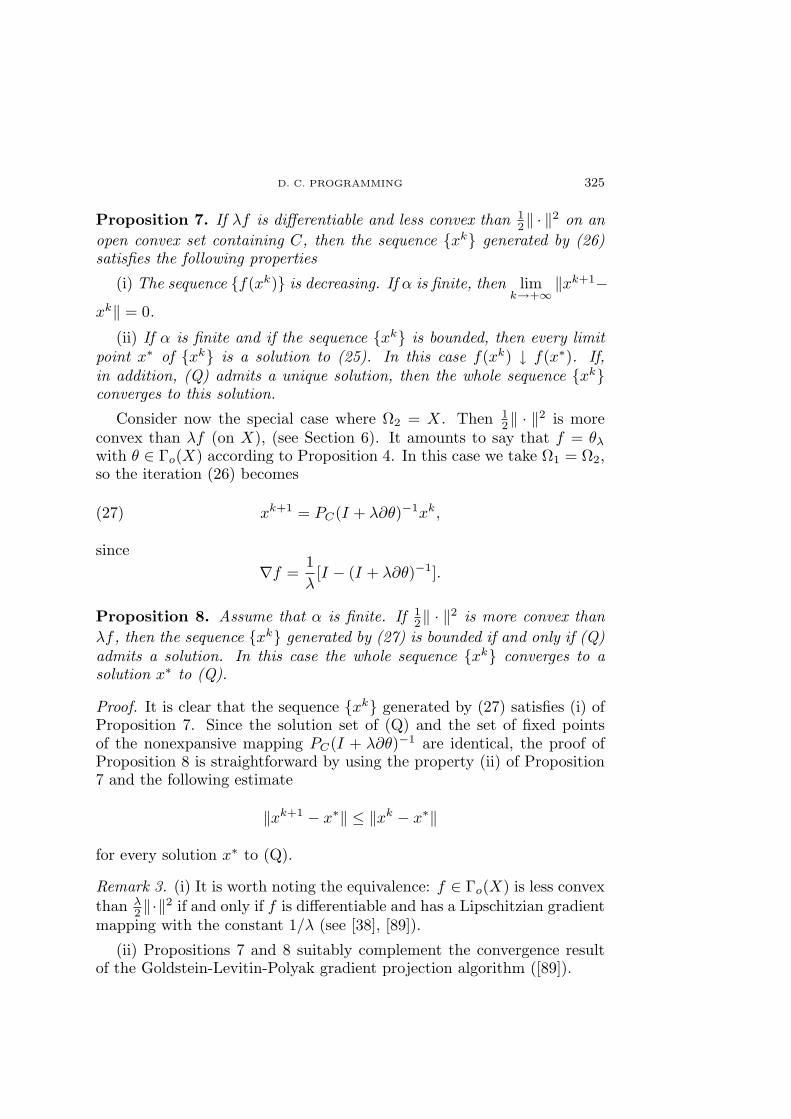
Proposition 7. If λf is differentiable and less convex than 12‖ · ‖2 on an
open convex set containing C, then the sequence xk generated by (26)satisfies the following properties
(i) The sequence f(xk) is decreasing. If α is finite, then limk→+∞
‖xk+1−xk‖ = 0.
(ii) If α is finite and if the sequence xk is bounded, then every limitpoint x∗ of xk is a solution to (25). In this case f(xk) ↓ f(x∗). If,in addition, (Q) admits a unique solution, then the whole sequence xkconverges to this solution.
Consider now the special case where Ω2 = X. Then 12‖ · ‖2 is more
convex than λf (on X), (see Section 6). It amounts to say that f = θλ
with θ ∈ Γo(X) according to Proposition 4. In this case we take Ω1 = Ω2,so the iteration (26) becomes
(27) xk+1 = PC(I + λ∂θ)−1xk,
since∇f =
1λ
[I − (I + λ∂θ)−1].
Proposition 8. Assume that α is finite. If 12‖ · ‖2 is more convex than
λf , then the sequence xk generated by (27) is bounded if and only if (Q)admits a solution. In this case the whole sequence xk converges to asolution x∗ to (Q).
Proof. It is clear that the sequence xk generated by (27) satisfies (i) ofProposition 7. Since the solution set of (Q) and the set of fixed pointsof the nonexpansive mapping PC(I + λ∂θ)−1 are identical, the proof ofProposition 8 is straightforward by using the property (ii) of Proposition7 and the following estimate
‖xk+1 − x∗‖ ≤ ‖xk − x∗‖
for every solution x∗ to (Q).
Remark 3. (i) It is worth noting the equivalence: f ∈ Γo(X) is less convexthan λ
2 ‖·‖2 if and only if f is differentiable and has a Lipschitzian gradientmapping with the constant 1/λ (see [38], [89]).
(ii) Propositions 7 and 8 suitably complement the convergence resultof the Goldstein-Levitin-Polyak gradient projection algorithm ([89]).
326 PHAM DINH TAO AND LE THI HOAI AN
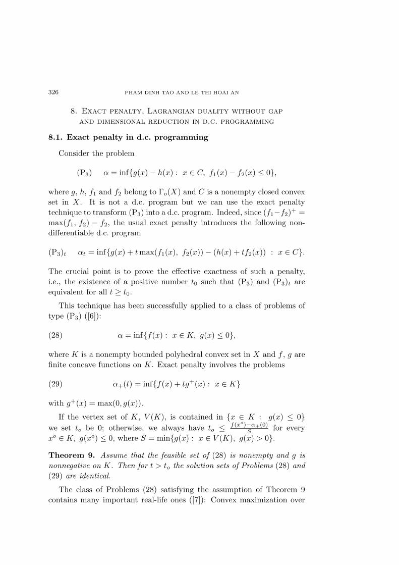
8. Exact penalty, Lagrangian duality without gap
and dimensional reduction in d.c. programming
8.1. Exact penalty in d.c. programming
Consider the problem
(P3) α = infg(x)− h(x) : x ∈ C, f1(x)− f2(x) ≤ 0,
where g, h, f1 and f2 belong to Γo(X) and C is a nonempty closed convexset in X. It is not a d.c. program but we can use the exact penaltytechnique to transform (P3) into a d.c. program. Indeed, since (f1−f2)+ =max(f1, f2) − f2, the usual exact penalty introduces the following non-differentiable d.c. program
(P3)t αt = infg(x) + t max(f1(x), f2(x))− (h(x) + tf2(x)) : x ∈ C.
The crucial point is to prove the effective exactness of such a penalty,i.e., the existence of a positive number t0 such that (P3) and (P3)t areequivalent for all t ≥ t0.
This technique has been successfully applied to a class of problems oftype (P3) ([6]):
(28) α = inff(x) : x ∈ K, g(x) ≤ 0,
where K is a nonempty bounded polyhedral convex set in X and f , g arefinite concave functions on K. Exact penalty involves the problems
(29) α+(t) = inff(x) + tg+(x) : x ∈ K
with g+(x) = max(0, g(x)).
If the vertex set of K, V (K), is contained in x ∈ K : g(x) ≤ 0we set to be 0; otherwise, we always have to ≤ f(xo)−α+(0)
S for everyxo ∈ K, g(xo) ≤ 0, where S = ming(x) : x ∈ V (K), g(x) > 0.
Theorem 9. Assume that the feasible set of (28) is nonempty and g isnonnegative on K. Then for t > to the solution sets of Problems (28) and(29) are identical.
The class of Problems (28) satisfying the assumption of Theorem 9contains many important real-life ones ([7]): Convex maximization over
D. C. PROGRAMMING 327
the Pareto set, bilevel linear programs, linear programs with mixed linearcomplementarity constraints, mixed zero-one concave minimization pro-gramming, etc.
8.2. Lagrangian duality without gap in d.c. programming
Let us present now two important results concerning the Lagrangianduality without gap in d.c. programming. The first deals with the maxi-mization of a gauge on the unit ball of another gauge.
Let ψ 6≡ 0 and φ 6≡ 0 be two finite gauges on X such that V = φ−1(0)is a subspace contained in ψ−1(0). Consider the following problem
(P1max) Sψφ(I) = supψ(x) : φ(x) ≤ 1,
which is equivalent to −Sψφ(I) = inf−ψ(x) : φ(x) ≤ 1.We consider the Lagrangian duality for this problem in the case where thefeasible domain is written as x ∈ X : (1/2)φ2(x) ≤ (1/2). We can write(P 1
max) in the form
(Pmax) α = −Sψφ(I) = inf− ψ(x) :
12φ2(x) ≤ 1
2
.
We will establish, like in a case of convex optimization, the stability in theLagrangian duality, namely, we will prove that there is no gap betweenthe optimal value of the primal and dual problems. These results allowus to obtain equivalent d.c. forms of (Pmax) and an explicit form of thegraph of the objective function for the dual problem. They can also beused for checking the globality of the solution computed by DCA.
Let U(φ) and S(φ) denote the unit ball and its sphere, respectively,i.e.,
U(φ) = x ∈ X : φ(x) ≤ 1; S(φ) = x ∈ X : φ(x) = 1.
First, we observe that the solution set of Problem (Pmax), denoted byPmax, is contained in S(φ), and the finiteness of Sψφ(I) implies φ−1(0) ⊂ψ−1(0).
Lemma 4 ([78], [84]). Pmax 6= ∅ and Problem (Pmax) is equivalent to
(PRmax) supψ(x) : x ∈ V ⊥, φ(x) ≤ 1,with Pmax = V + PRmax, where PRmax is the solution set of (PRmax).

328 PHAM DINH TAO AND LE THI HOAI AN
Proof. Since X = V +V ⊥, for every x ∈ X we have x = u+v, u ∈ V , wherev ∈ V ⊥. Thus, ψ(x) = ψ(u + v) = ψ(v), φ(x) = φ(u + v) = φ(v), whichimplies that Pmax is equivalent to (PRmax). Since x ∈ V ⊥ : φ(x) ≤ 1 iscompact, the solution set of (PRmax) is nonempty. Furthermore, Pmax =V + PRmax.
The Lagrangian L(x, λ) for (Pmax) is given by
L(x, λ) = −ψ(x) + λ
2 (φ2(x)− 1) if λ ≥ 0,
−∞, otherwise.
Clearly, −ψ(x) + χC(x) = supL(x, λ) : λ ≥ 0. Thus, (Pmax) can bewritten as
α = −Sψφ(I) = infsupL(x, λ) : λ ≥ 0 : x ∈ X.
For λ ≥ 0 we have
(Pλ) γ(λ) = inf− ψ(x) +
λ
2(φ2(x)− 1) : x ∈ X
.
As for (Pmax), solving (Pλ) amounts to solving
(PRλ) γ(λ) = inf− ψ(x) +
λ
2(φ2(x)− 1) : x ∈ V ⊥
knowing that Pλ = V + PRλ.
It is clear that γ is a concave function and (Pλ) is a d.c. optimizationproblem.
The dual problem of (Pmax) is
(D) β = supγ(λ) : λ ≥ 0 = supinfL(x, λ) : x ∈ X : λ ≥ 0.
By the definition of Lagrangian we have
α = infsupL(x, λ) : λ ≥ 0 : x ∈ X≥ supinfL(x, λ) : x ∈ X : λ ≥ 0 = β.(30)
A point (x∗, λ∗) ∈ X × IR is said to be a saddle point of L(x, λ) if
L(x∗, λ) ≤ L(x∗, λ∗) ≤ L(x, λ∗), ∀(x, λ) ∈ X × IR.
Let us state now important results concerning characterization of solutionsof the dual problem and the stability of the Lagrangian duality.
D. C. PROGRAMMING 329
Theorem 10 ([78]). (i) Pλ 6= ∅ for every λ > 0 and dom γ =]0,+∞[.
(ii) D 6= ∅ and γ(λ) = −λ2 + K
λ , where K is a negative constant (depen-dent only on ψ and φ).
(iii) D = λ∗ = √−2K, γ(λ∗) = −λ∗.
(iv) α = β and Pmax = Pλ∗ .
(v) (x∗, λ∗) ∈ Pmax × D if and only if (x∗, λ∗) is a saddle point ofL(x, λ).
(vi) Pmax = x∗φ(x∗) : x∗ ∈ P1.
Consider now Problem (Pλ) with λ = 1.
(P1) γ(1) +12
= inf1
2φ2(x)− ψ(x) : x ∈ X
.
The following result allows determining a new d.c. optimization problemwhich is equivalent to (Pmax).
Theorem 11 ([78]).
(31) P1 = ψ(x∗)x∗ : x∗ ∈ Pmax.The second result concerns the minimization of a quadratic form on
Euclidean balls (the so-called trust region subproblem) or spheres
α1 = min
q(x) =12xT Ax + bT x : ‖x‖ ≤ r,(32)
α2 = min
q(x) =12xT Ax + bT x : ‖x‖ = r
,(33)
where A is an n×n real symmetric matrix, b ∈ IRn, r is a positive numberand ‖ · ‖ denotes the Euclidean norm of IRn.
We present first the results concerning the stability of the Lagrangianduality for Problem (32). To this end, we rewrite (32) as
α1 = min
q(x) :12‖x‖2 ≤ r2
2
.
Theorem 12 ([82]). (i) α1 = β1.
(ii) The dual problem has a unique solution λ∗ and the solution set ofthe primal problem (32) is the set
x∗ ∈ Pλ∗ : ‖x∗‖ ≤ r, λ∗(‖x∗‖ − r) = 0.As an immediate consequence we obtain the well-known optimality con-dition for (32) whose proof is not trivial.

330 PHAM DINH TAO AND LE THI HOAI AN
Corollary 5 ([63], [77], [82]). x∗ is a solution to (32) if and only if thereexists λ∗ ≥ 0 such that
(i) (A + λ∗I) is positive semi-definite,
(ii) (A + λ∗I)x∗ = −b,
(iii) λ∗(‖x∗‖ − r) = 0, ‖x∗‖ ≤ r.
Such a λ∗ is the unique solution to the dual problem.
By the same approach we obtain analogous results for Problem (33). Thesole difference between these problems is that λ∗ is not assigned to benonnegative in the latter.
Remark that Problems (32) and (33) are among a few nonconvex op-timization problems which possess a complete characterization of theirsolutions. These problems play an important role in optimization and nu-merical analysis ([1], [19], [31], [63], [77], [82], [83], [86], [98], [99], [100]).
8.3. Dimensional reduction technique in d.c. programming
Let h ∈ Γo(X) and h0+ be its recession function ([93]). The linealityspace of h is denoted by [93]
L(h) = u ∈ X : h0+(u) = −h0+(−u).
It is a subspace of the direction u in which h is affine:
h(x + λu) = h(x) + λν, ∀x ∈ X, ∀λ ∈ IR,
where h0+(u) = −h0+(−u) = ν. We have dim L(h) + dim h∗ = n. Moreprecisely, we have the following decomposition ([93])
X = V + V ⊥,
where V is the subspace parallel to the affine hull of dom h∗ (denotedby aff(dom h∗)), and V ⊥ is exactly L(h). The function h can then bedecomposed as
h(a + b) = h(a) + 〈w, b〉,where (a, b) ∈ V × V ⊥ and w is an arbitrary element of aff(dom h∗). Inother words, if P is an n×p matrix and Q is an n×q matrix such that the

D. C. PROGRAMMING 331
columns of P (resp. Q) constitue an orthonormal basis of V (resp. V ⊥),then we have
x = a + b = Pu + Qv, u ∈ IRp, v ∈ IRq;
h(x) = h(Pu + Qv) = h(Pu) + 〈QT w, v〉.
A d.c. program
(P) α = infg(x)− h(x) : x ∈ X
is said to be weakly nonconvex, if p = dim h∗ is small. In this case wehave
f(x) = g(x)− h(x) = g(Pu + Qv)− h(Pu + Qv)
= g(Pu + Qv)− 〈QT w, v〉 − h(Pu).
The nonconvex part of f(Pu + Qv) appears only in h(Pu) which simplyinvolves p dimensions. The dimensional reduction technique can improveDCA’s qualities. It also permits global algorithms to treat large scaleweakly nonconvex d.c. programs.
9. Applications
We present in this section the d.c. approach to some important non-convex problems that DCA have been successfully applied to.
9.1. DCA for globally solving the trust region subproblem (TRSP)
Recall that TRSP is the problem of the form (32)
α1 = min
q(x) =12xT Ax + bT x : ‖x‖ ≤ r
.
J. M. Martinez ([60]) has investigated the nature of local-nonglobal solu-tions of TRSP and shown the following property: TRSP has at most onelocal nonglobal solution. Moreover, being inspired by G.E. Forsythe &G.H. Golub’s work ([28]), S. Lucidi et al. ([55]) have stated a very niceresult: in TRSP the objective function can admit at most 2m+2 different
332 PHAM DINH TAO AND LE THI HOAI AN
values at Kuhn-Tucker points, where m is the number of distinct negativeeigenvalues of A.
Clearly, this problem is a d.c. program with different d.c. decomposi-tions. Let us point out some examples, which are of particular interest.
(i) f(x) = g(x)− h(x) with
g(x) =12〈A1x, x〉+ 〈b, x〉+ χC(x),
andh(x) =
12〈A2x, x〉.
The matrices A1 and A2 are symmetric positive semidefinite related tothe spectral decomposition of A: A = A1 −A2 with
A1 =∑
i∈K
λiuiuTi , A2 = −
∑
i∈L
λiuiuTi .
Here λ1 ≤ . . . ≤ λn are the eigenvalues of A and u1, . . . , un is anorthonormal basis of IRn constituted by corresponding eigenvectors of A,K := i : λi ≥ 0, L := i : λi < 0, C := x ∈ IRn : ‖x‖ ≤ r.
(ii) f(x) = g(x)− h(x) with
g(x) =12〈(A + ρI)x, x〉+ 〈b, x〉+ χC(x),
andh(x) =
12ρ‖x‖2.
The positive number ρ is chosen such that the matrix A + ρI is positivesemidefinite, i.e., ρ ≥ −λ1.
(iii) f(x) = g(x)− h(x) with
g(x) =ρ
2‖x‖2 + 〈b, x〉+ χC(x),
andh(x) =
12〈(ρI −A)x, x〉.
The positive number ρ, in this case, should render the matrix ρI − A
positive semidefinite, i.e., ρ ≥ λn.

D. C. PROGRAMMING 333
We can describe without any difficulty the corresponding DCA. How-ever, for these decompositions, we see that DCA is explicit in the case (iii)only:
yk = (ρI −A)xk → xk+1 = PC(xk − 1ρ(Axk + b)).
Here PC is the orthogonal projection mapping on C.
From the computational viewpoint, a lot of our numerical experimentsproved the robustness and the efficiency of DCA with respect to the otherwell known algorithms, especially in the large scale trust-region subprob-lems ([83], [96], [99]).
9.2. DCA for solving the Multidimensional scaling problem(MDS)
The Multidimensional Scaling Problem (MDS) has a fundamental rolein statistics by various applications in different fields such as social sciences([13]), biochemistry ([21], [22]), psychology ([52]), mathematical psychol-ogy ([11], [97]), etc. The mathematical formulation of this importantproblem, due to Kruskal ([50]), is as follows:
Let φ be a norm on IRp and d be its corresponding metric. For an n×p
matrix X we define
dij(X ) = d(X Ti ,X T
j ) = φ(X Ti −X T
j ),
where Xi is the ith row of X .
Let two matrices ∆ = (δij) and W = (wij) of order n be given suchthat
δij = δji ≥ 0 , wij = wji ≥ 0 , ∀i 6= j; δii = wii = 0 ∀i, j = 1, . . . , n.
The normal case corresponds to wij = 1, ∀i 6= j. We shall refer to ∆as the dissimilarity matrix and W as the weight matrix. A metric MDSproblem consists of finding in IRp n objects X1, . . . , Xn, representing ann× p matrix X , such that the differences | d(Xi,Xj)− δij | for every i andj are smallest.
Let Mn,p(IR) denote the space of all real matrices of order n× p. Themathematical form of metric MDS problem then can be written as
(MDS) σ∗ = min
σ(X ) =
12
∑
i<j
wijθ(δij − dij(X )) : X ∈Mn,p(IR)
,
334 PHAM DINH TAO AND LE THI HOAI AN
where θ(t) = |t| (resp. t2) for t ∈ IR.
Other mathematical models have been discussed in [50], [102]. Theclassical metric MDS problem corresponds to θ(t) = t2 ([50]). The func-tion σ is called the loss function. So, this problem is also sometimesreferred to as the distance geometry problem. Semidefinite programmingproblems have been formulated by multidimensional and clustering tech-niques in [61]. Recently similar models have been used for the moleculeproblem [34], the protein structure determination problem ([116], [117])and the protein folding problem ([30]). Some gradient-type methods weredeveloped by J.B. Kruskal [48], [49], L. Gutman [33], J.C. Lingoes, E.E.Roskam [53] for solving this problem. These gradient-type methods failto use if the loss function σ is nondifferentiable ([24], [25]).
In 1977 J. de Leeuw [24] proved that the classical metric MDS problemis equivalent to the convex maximization problem given as
(Smax) max
ρ(X )η(X )
: η(X ) 6= 0⇔ max ρ(X ) : η(X ) ≤ 1 ,
where
η(X ) =
∑
i<j
wijd2ij(X )
1/2
and ρ(X ) =∑
i<j
wijδijdij(X )
are two seminorms in Mn,p(IR). So, the classical MDS problem is reducedto the problem of maximization of the semi-norm ρ on the unit ball definedby the seminorm η. For solving the metric Euclidean MDS with θ(t) = t2
de Leeuw proposed an algorithm [24] (see also [25]), called the majoriza-tion method, similar to Guttman’s C-matrix method whose convergenceresult has been stated by following the same scheme of the subgradientmethod (for maximizing a semi-norm on the unit ball of another semi-norm) which has been studied extensively in the general framework ofconvex analysis by Pham Dinh Tao ([70]-[74]). De Leeuw merely usedthe subgradient method ([70]-[74]) for solving the classical metric MDSproblem with noneuclidean norm φ ([24]). In the Euclidean case de Leeuwobserved judiciously that his elegant adapted algorithm is unlike the sub-gradient method since lim
k→+∞‖X k+1 − X k‖ is not necessarily zero in the
former. In fact, such a property can be obtained by applying regular-ization techniques to subgradient methods (see Section 5). De Leeuw’salgorithm has been so successful that it has become a reference method
D. C. PROGRAMMING 335
to the classical metric Euclidean MDS problem (θ(t) = t2). Remark thatde Leeuw’s approach fails to use in the case where θ(t) = |t|.
(MDS) with θ(t) = t2 in fact is a d.c. optimization problem of the form
(34) (S1) min
12η2(X )− ρ(X ) : X ∈Mn,p(IR)
,
since
σ(X ) =12
∑
i<j
wijd2ij(X ) +
∑
i<j
wijδ2ij −
∑
i<j
wijδijdij(X )
=12η2(X )− ρ(X ) +
∑
i<j
wijδ2ij .
It has been proved in [84] that the seminorms η and ρ can be expressed as
η(X ) =12〈TX ,X〉, ρ(X ) =
12〈B(X )X ,X〉,
where the matrices T = (tij) and B(X ) = (bij(X )) are defined by
tij =
−wij if i 6= j,n∑
j=1
wij if i = j.bij =
−wijδijsij(X ) if i 6= j,
−n∑
j=1,j 6=i
bij if i = j.
sij(X ) =
1/(‖X Ti −X T
j ‖) ifXi 6= Xj ,
0 otherwise.
The stability of the Lagrangian duality for Problem (Smax) (Subsection8.2) permits finding various d.c. decompositions for this problem, in par-ticular, the equivalence of (Smax) and (S1). Moreover, the expression ofthe dual objective function can be used to check the globality of solutionscomputed by DCA.
Solving Metric MDS Problem by DCA:
Let A denote the set of matrices in Mn,p(IR) whose rows are identical,i.e.,
A := X ∈ Mn,p(IR) : X1 = · · · = Xn.It is a subspace of Mn,p(IR). Its orthogonal subspace is A⊥ = Y ∈Mn,p(IR) :
n∑i=1
Yi = 0.

336 PHAM DINH TAO AND LE THI HOAI AN
We can assume, without loss of generality, the irreducibility of theweight matrix W , otherwise the MDS problem can be decomposed intoa number of smaller problems. We will give below the description DCAapplied to (S1) and (Smax) for solving the metric MDS problem with θ(t) =t2 and the Euclidean norm φ. Problems (S1) and (Smax) then take theform (P1) and (Pmax), where the semi-norms ρ and η replace the gaugesψ and φ, respectively (Subsection 8.2)
From the stability results obtained in the last section (Theorem 11)solving Problem (P1) amounts to solving (Pmax)(35)(Pmax) maxρ(X ) : η(X ) ≤ 1 ⇔ minχC(X )− ρ(X ) : X ∈Mn,p(IR),
where C = X ∈ Mn,p(IR) : (1/2)η2(X ) ≤ 1/2. The last is a d.c.program.
Now we describe DCA (with and without regularization) for solvingProblems (P1) and (Pmax). First, observe that for both (P1) and (Pmax)we can restrict ourselves within to A⊥, where each of these problems hasalways a solution ([1], [84]).
The DCA applied to (P1) and (Pmax) is reduced to calculating sub-differentials of the functions ρ, ((1/2)η2)∗, χ∗C , [(λ/2)η2 + (µ/2)‖.‖2]∗ and[λχC + (µ/2)‖.‖2]∗.
We have first calculated these subdifferentials for the general case andthen particularized the results in the normal case (wij = 1, ∀i 6= j) ([1],[84]).
Let ε > 0, λ > 0, µ > 0 and X o ∈ A⊥ be given.
Let k = 0, 1, . . . until ‖X k+1 −X k‖ ≤ ε.
DCAP1: Take X k+1 = B(Xk)Xk
n
RDCAP1: Take X k+1 = (λB(Xk)+µI)Xk
µ+λn
DCAPmax: Take X k+1 = B(Xk)Xk
η(B(Xk)Xk)
RDCAPmax: Take X k+1 =
(λB(Xk)+µI)Xk
µ , if η((λB(X k)
+µI)X k) ≤ µ,
(λB(Xk)+µI)Xk
η((λB(Xk)+µI)Xk), otherwise.
∣∣∣∣∣∣∣∣∣∣∣∣∣∣∣∣∣∣∣∣∣∣∣∣∣∣∣∣∣∣∣∣∣∣∣∣∣∣∣∣∣∣∣∣∣∣∣∣∣∣∣∣∣∣

D. C. PROGRAMMING 337
Recall that η(Y) =√
n‖Y‖ in DCAPmax and RDCAPmax.
The original d.c. decomposition for the objective function of (P1) in(34) seems to be better than the corresponding one relative to (Pmax) in(35). As direct consequences of the above description of DCA, we have:
(i) Without computing the denominator in each step, DCAP1 (resp.RDCAP1) is less expensive than DCAPmax (resp. RDCAPmax), and thedifference of the cost is proportional to the dimension n× p of (MDS).
(ii) On the practical point of view, the first two algorithms are obivouslymore stable than the last ones, especially in large-scale MDS problems.
These observations have been justified by many numerical simulations.Let us point out now the fact that de Leeuw’s algorithm for solving themetric Euclidean MDS problem (in the case where the weight matrix issupposed to be irreducible) is a special case of DCA applied to the d.c.program (P1). Indeed DCAP1 is given by (for a given X o ∈ A⊥)
X k+1 = T+B(X k)X k ∈ A⊥,
where the computation of X = T+Y with Y ∈ A⊥ amounts solving thenonsingular linear system (T + (1/n)eeT )X = Y ([1], [84]) We rediscoverthus de Leeuw’s algorithm [24], [25].
Normal metric Euclidean MDS as parametrized trust region subproblemsand its solution by the parametrized DCA
The particular structure of the seminorms η and ρ have enabled us toformulate the normal metric Euclidean MDS problem (P1) as parametrizedtrust region subproblems and to devise the parametrized DCA for solving(P1). This approach is promising because the DCA is robust and efficientfor globally solving the trust region subproblem ([83]).
It is worth noting that if the rugularization parameter is fixed, thenthe corresponding parametrized DCA is reduced to RDCAPmax.
9.3. DCA for solving a class of linearly constrained indefinitequadratic problems
We consider the indefinite quadratic problem over a bounded poly-hedral convex set which plays an important role in global optimization:
(IQP1) min1
2〈Hx, x〉+ 〈l, x〉 : x ∈ K.
Here H is a symmetric indefinite q × q-matrix, l ∈ IRq, K is a nonemptybounded polyhedral set defined as K = x ∈ IRq : Ax ≤ a, x ≥ 0 with

338 PHAM DINH TAO AND LE THI HOAI AN
A being an m× q-matrix, a ∈ IRm. When
H =(
C 00 D
)
and the polytope is defined as
Ω = (x, y) ∈ IRn×IRs : Ax+By ≤ a, A1x ≤ a1, A2y ≤ a2, x ≥ 0, y ≥ 0
we have the problem
(IQP2) min
F (x, y) =12〈Cx, x〉+〈c, x〉+1
2〈Dy, y〉+〈d, y〉 : (x, y) ∈ Ω
.
Here, C is a symmetric positive semi-definite n × n-matrix, D is a sym-metric negative semi-definite s × s-matrix, c ∈ IRn, d ∈ IRs, and A is anm× n-matrix, B is an m× s-matrix, A1 is an r× n-matrix, A2 is a p× s-matrix, a ∈ IRm, a1 ∈ IRr, a2 ∈ IRp. So the objective function of (IQP2)is decomposed in a sum of a convex part and a concave part. A specialcase of (IQP2) is the problem where D is diagonal (i.e., the concave partis separable):
(IQP3) min
f(x, y) =12〈Cx, x〉+ 〈c, x〉+
s∑
i=1
[diyi − 12λiy
2i ] : (x, y) ∈ Ω
with λi > 0.
Problem (IQP1) is in fact a problem of the form (IQP3). Likewise, Problem(IQP2) can be equivalently transformed into a problem of the form (IQP3)where the concave variable is separable.
When C ≡ 0 in (IQP3) and the polytope is defined as
Ω = (x, y) ∈ IRn × IRs : Ax + By ≤ a, x ≥ 0, y ≥ 0,
we have the linearly constrained concave quadratic problem which havebeen considered by several authors (see e.g. Rosen and Pardalos [92],Kalantari and Rosen [45], Pardalos et al. [66], Phillips and Rosen [88],etc.). In this case the global minimum point is always attained at leastat a vertex of the convex polytope Ω. This property is no longer truewhen C 6≡ 0. Hence, Problem (IQP3) with C 6≡ 0 is likely even moredifficult to be numerically solved than concave programs. Recently, adecomposition branch-and-bound method for dealing with (IQP3) in thecase where C 6≡ 0 was proposed in Phong-An-Tao [103]. This method

D. C. PROGRAMMING 339
based on normal rectangular subdivisions which exploit the separabilityof the concave part in the objective function. In general, the existingalgorithms are efficient if the number of the concave variables is small.
Clearly, Problem (IQP2) can be considered as minimization of a d.c.function over a polytope for which some method developed in global ap-proaches (see e.g., Horst et al. [41], Tuy [112]) can be applied. For solving(IQP2) in the case where the number of variables is large, we should avoidthe inherent difficulties of this global optimization problem by using localapproaches. We proposed a “good” d.c. decomposition for which nume-rical experience indicates that the DCA is efficient for solving (IQP2).In contrast to global algorithms whose complexity increases exponentiallywith the dimension of the concave variable, DCA has the same behaviourwith respect to both dimensions of convex variables and concave variables.Consequently, they solve these problems when the number of concave vari-ables is large. For solving (IQP1) we presented some d.c. decompositionsand their corresponding DCA which seem to be efficient. We proposed alsoa decomposition branch-and-bound method for globally solving (IQP1)and (IQP2). These methods are just a modification of the one in Phong-An-Tao [103] for the general case. We used these algorithms for checkingthe globality of the solution computed by DCA when s ≤ 30. Computa-tional experiments proved that
• The global algorithms only run until s = 30. The DCA is much fasterthan the global algorithm (until 30 times).
• In most problems the DCA gave global solutions.
• The DCA terminated very rapidly; the average number of iterationsis 15.
9.4. A branch-and-bound method via D.C. Optimization Algo-rithms and Ellipsoidal technique for Nonconvex Quadratic Prob-lems
For simplicity we present only the algorithm for solving box constrainednonconvex quadratic problems [3] (see [8]) for the general nonconvex qua-dratic program):
(QB) min
f(x) :=12〈x,Ax〉+ 〈b, x〉 :
−∞ < li ≤ xi ≤ ui < +∞, i = 1, . . . , n
,

340 PHAM DINH TAO AND LE THI HOAI AN
with A being an n× n symmetric matrix, b, x ∈ IRn.
A special case of (QB) is the unconstrained quadratic zero-one problemwhich has many important applications, particularly in combinatorial op-timization, looks as follows
(36) min
f(x) :=12〈x,Ax〉+ 〈b, x〉 : x ∈ 0, 1n
.
Indeed, writing (36) in the form
(37) min
12〈x, Ax〉+ 〈b, x〉+
t
2(〈e, x〉 − 〈x, x〉) : x ∈ 0, 1n
,
we have
(38) (37) ⇔ min
12〈x, (A− tI)x〉+ 〈b +
t
2e, x〉 : x ∈ [0, 1]n
,
where e is the vector of ones and t is a real scalar such that A − tI isnegative semidefinite.
Several algorithms have been proposed for globally solving these prob-lems (see e.g. [10], [42], [43], [67], [68], [90]). The procedures often usedin the existing methods are to relax the constraints and perturb the ob-jective function. The branching is usually based upon rectangular and/orsimplicial partitions.
Ellipsoidal techniques have been used to state estimations for optimalvalues in nonconvex quadratic programming ([114], [115]). In [114] anapproximation algorithm was proposed for finding an ε-approximate solu-tion. It was shown that such an approximation can be found in polynomialtime for fixed ε and t, where t denotes the number of negative eigenvaluesof the quadratic term.
We have proposed a combined branch-and-bound algorithm and DCAfor solving (QB). The aim of DCA is here twofold. The first use dealswith the lower bound computation scheme. We apply DCA to solve theproblem (QE) which is obtained from (QB) by replacing the rectangleconstraint with an ellipsoid containing the selected rectangle. Our mainmotivation for the use of this technique is that DCA is very efficient forglobally minimizing a quadratic form over an euclidean ball ([1], [83]). Thesecond use concerns the upper bound computation process. For finding
D. C. PROGRAMMING 341
a good quality of feasible solutions we apply DCA to solving (QB) fromgood starting points which are obtained during computing lower bounds.
The global algorithm we are going to describe starts with an ellipsoidE0 containing the feasible region K0 of (QB). If a minimizer of f overE0 is feasible then we stop the process. Otherwise, we divide K0 intotwo rectangles (rectangular bisection) and construct two ellipsoids suchthat each of them contains one of the just divided rectangles. To improvethe lower bound we compute minimums of f on each newly generatedellipsoid. The procedure is then repeated by replacing K0 by a rectan-gle corresponding to the smallest lower bound and E0 with an ellipsoidcontaining this rectangle. As this procedure repeats infinitely many timestwo infinite nested sequences of rectangles and ellipsoids are generated andshrink to a singleton. The convergence of the algorithm thus is ensured.
For computing lower bounds, we are concerned with the constructionof a sequence of ellipsoids Ek such that:
(i) Ek contains the current rectangle Kk,
(ii) the volume vol(Ek) decreases to zero as k → +∞,
(iii) the lower bounds (supplied by the solution of (QE) defined below)are sufficiently tight.
The lower bound of f in our algorithm is improved by the solution ofthe problem
(QE) min
12〈x,Ax〉+ 〈b, x〉 : x ∈ X
.
Again by the transformation L one has x ∈ X if and only if y = Lx ∈ S,so the last problem is equivalent to the trust region subproblem
(39) min
12〈y, D−1AD−1y〉+ 〈D−1q −D−1AD−1c, y〉 : ‖y‖2 ≤ n
.
Clearly, D−1AD−1 is an n × n symmetric matrix. The DCA is used forglobally solving (39).
The main contribution of our method is to give a good combinationbetween the local and global approaches: first, we have provided a simpleand efficient algorithm using the information of the bounding procedure forfinding good local minima of box constrained quadratic problem; secondly,we have used the elippsoidal technique for bounding based on an efficient
342 PHAM DINH TAO AND LE THI HOAI AN
algorithm (DCA) for the ball constrained quadratic problem. We havestudied also the new branching procedure in rectangular partition in orderto well adapt to the new ellipsoidal bounding technique.
Preliminary experiments showed the efficiency as well as the limit ofour algorithm. The advantages are that either an ε-optimal solution or agood feasible point is obtained rapidly by the DCA and thereby a consid-erable number of generated ellipsoids are deleted from further considera-tion. Therefore, in general the algorithm is efficient for a proper choiceof tolerance ε (nevertheless this choice does not present always exactlythe quality of the solution obtained, see, e.g., Table 6 in [3]). Moreover,it is very efficient for some classes of problems: it could treat until thedimension 1000 (Tables 1, 2, 3 in [3]). Again, the DCA for subproblemsin bounding procedures are explicit and not expensive. The limit is that,as often happened in a branch-and-bound algorithm, the lower bound isimproved slowly. That is why we introduced the second process of lowerbounding in such a case. In the study of the performance of our algorithm,an open question is that which ellipsoid can be chosen to warrant the bestinitial lower bound? Meanwhile our ellipsoid technique seems to be quitesuitable.
9.5. DCA for globally solving nonconvex quadratic programming
We consider the general nonconvex quadratic programming
(QP) inf
f(x) =12〈Ax, x〉+ 〈b, x〉 : Bx ≤ c
,
with A being an n × n symmetric matrix, B being an m × n matrix andb ∈ IRn, c ∈ IRm.
As in the TRSP, Kuhn-Tucker points of nonconvex quadratic program(QP) enjoy the following nice property due to Bomze & Danninger ([15]):the objective function f can be assume at most 2m + 1 different values atKuhn-Tuker points of (QP).
We associate with the DCA (for solving nonconvex quadratic programs)an escaping procedure based on the trust region method ([63], [64], [77],[98]) for globally solving (QP). This is proceeded as follows:
Let x∗ be a Kuhn-Tucker point computed by the DCA and let ε be apositive number. Consider the linear quadratic equations
(40)
f(x) = f(x∗)− ε,
Bx + v2 = c,

D. C. PROGRAMMING 343
where v = (v1, . . . , vm) ∈ IRm and v2 denotes the vector v = (v21 , . . . , v2
m).
If the Kuhn-Tucker point x∗ is not a global solution to (QP), thenfor ε sufficiently small there exists a solution (x, v) to (40) which can becomputed by the trut region methods with the starting point (x∗, v∗),where v∗2 = c − Bx∗. In this case we must restart DCA with the newinitial point x.
Finally, the DCA (with at most 2m+1 restarting procedures) convergesto a global solution of (QP).
9.6. D.c. approach for linearly constrained quadratic zero-oneprogramming problems
We are interested in solving the well-known linearly constrained qua-dratic zero-one programming
(01QP) α = min
f(x) :=12xT Cx + cT x : Ax ≤ b, x ∈ 0, 1n
,
where C is an (n × n) symmetric matrix, c, x ∈ IRn, A is an (m × n)matrix and b ∈ IRm.
This problem, which is a key one in combinatorial optimization, is NP-hard and has been extensively investigated by several authors. A specialcase of this is linear zero-one programming which has many important ap-plications in economics, planning and various kinds of engineering design.We propose a new algorithm in a continuous approach for the followingequivalent concave minimization problem
(CCQP) α = min
12xT (C − λI)x + (c +
λ
2e)T x : Ax ≤ b, x ∈ [0, 1]n
,
where e is the vector of ones and λ ≥ λo > 0 (see Section 8.1 and [7]).
Clearly, (CCQP) is a d.c. program to which some global methods canbe applied (see e.g. [41], [112]), when the dimension is small. For largescale setting it would be interesting to use the DCA for solving (CCQP).
In order to guarantee that solutions computed by the DCA are globalwe introduce a branch-and-bound scheme. With this purpose, first wetransform (CCQP) into the d.c. program with the separable concave part
(DCQP) α = ming(x)− h(x) : x ∈ K.

344 PHAM DINH TAO AND LE THI HOAI AN
Here K = x ∈ IRn : Ax ≤ b, 0 ≤ xi ≤ 1, i = 1, . . . , n,
(41) g(x) :=12xT (C + (ρ− λ)I)x + (c +
λ
2e)T x; h(x) :=
12ρ
n∑
i=1
x2i ,
and ρ is a positive number such that the matrix (ρ − λ)I + C is semipositive definite. The branch-and-bound algorithm is in fact consideredfor the problem (DCQP). It aims to find a good starting point for theDCA and, naturally, to prove the globality of the solutions obtained bythe DCA. This combination of two approaches improves the qualities of theDCA and accelerates the convergence of the branch-and-bound algorithm.
We note that the equivalence between (01QP) and (CCQP) is not un-usual. Neverthelesse the existing algorithms for solving the last problemare not often applied in the solution of the former. The reason is that, inpractice a branch-and-bound scheme (in a continuous approach) is oftenused for finding an ε-solution of the problem being considered, since it isvery difficult to obtain an exact solution. Unfortunetly, such an ε-solutionof (CCQP) may be not integer. However, the DCA applied to (CCQP)with t sufficiently large provides a point in 0, 1n. This advantage ofthe DCA makes our method efficient in finding an integer ε-solution of(DCQP) in large scale setting.
Preliminary computational experiences [5] showed that the DCA is veryefficient: it provides either an optimal solution or a good approximationto it within some first iterations. As for the branch-and-bound algorithm,it works very well in linear zero-one programming. In case of quadraticprogramming, when n > 40, to ensure the globality the algorithm neededmuch more iterations. Another procedure for improving lower bounds inthis case is currently under the research.
9.7. DCA for optimizing over the efficient set
Let C be a p×n real matrix, and K be a nonempty compact convex setof IRn. Let f be a real valued function on IRn. An optimization problemover the efficient set is that of the form
(42) maxf(x) : x ∈ KE.Here KE denotes the Pareto set of the following multiple objective pro-gramming problem:
(MP) maxCx : x ∈ K.

D. C. PROGRAMMING 345
We recall that a point x0 is said to be an efficient point of Problem (MP)when x0 ∈ K, and whenever Cx ≥ Cx0 for some x ∈ K, then Cx = Cx0.
Following [12] for each x we define p(x) as
(Lx) p(x) := maxeT C(y − x) : Cy ≥ Cx, y ∈ K,where e is the row vector in IRp whose all entries are 1. It is clear thatthe effective domain of −p is the projection on IRn of (x, y) ∈ IRn ×K : Cx − Cy ≤ 0 which contains K. This function has the followingproperties:
Lemma 5 ([6], [7]). (i) p is nonnegative on K, and x ∈ KE if and onlyif p(x) = 0, x ∈ K.
(ii) p is upper semicontinuous concave function on the whole space.
(iii) If, in addition, K is polyhedral convex, then p is polyhedral concaveon K.
In virtue of Lemma 5, Problem (P) can be written as
(P’) maxf(x) : p(x) ≤ 0, x ∈ K.Since p(x) ≥ 0 for every x ∈ K, and p(x) = 0, x ∈ K if and only ifx ∈ KE , this function is an exact penalty function (with respect to K).Thus, the corresponding penalized problem is
(43) mintp(x)− f(x) : x ∈ K.According to Theorem 9, if f is convex, then there is a nonnegative numberto such that (42) and (43) are equivalent for t > to.
Remark that (43) is a polyhedral d.c. program if f is concave. More-over, if f is linear and the vertex set of K, V (K), is not contained inKE , then for t > (U0 − f(x0))/M0, with U0 := maxf(x) : x ∈ K andM0 := minp(x) : x ∈ V (K), p(x) > 0 > 0, the sequence xk generatedby DCA are in KE provided the starting point x0 is efficient.
Numerous computational experiments proved that ([6])
1. For DCA:
• DCA terminates very rapidly; average number of iterations is 3.
• DCA works with problems where the number of the criteria may belarge. The running times are relatively insensitive to the increase of thenumber of the criteria.

346 PHAM DINH TAO AND LE THI HOAI AN
• The optimal value computed by DCA depends on the initial point. Ingeneral the optimal value is close to the global optimal value if the initialpoint x0 is chosen as
x0 = γx + (1− γ)xmax, 0.5 < γ < 1,
wherex = argmaxλCx : x ∈ K, with λ ∈ V (S0),
xmax = argmaxf(x) : x ∈ K.Although this initial point in general is not efficient, the computed solu-tions always are efficient.
• The algorithms are unstable if the penalty parameter is large.
2. For global algorithms (a combination of DCA and a based branch-and-bound global algorithm)
• The algorithm is efficient only if the number of the criteria is small,since the running time is very sensitive to the increase of the number ofthe criteria.
• In general, after a reasonable number of iterations a global solutionis reached. To detect its globality, however, we need much more itera-tions. The reason is that the upper bounds are not sufficiently sharp, andsometimes they are improved very slowly.
9.8. Linear and nonlinear complementarity problems. Differenceof subdifferentials complementarity problem
Consider the problem of the form
(NLC)
Find (x, y) ∈ IRn × F (x) such thaty ≥ 0 and 〈x, y〉 = 0,
where F is an operator defined on IRn.
If F (x) = (f1(x), . . . , fn(x))T is a d.c. vector-function (i.e., its compo-nents fi are d.c.), then it is well-known that ([44]) (NLC) is equivalent tothe following nonconvex program type (3) (Introduction)
0 = inf
n∑
i=1
min (xi, fi(x)) : x ≥ 0, fi(x) ≥ 0, i = 1, . . . , n
.

D. C. PROGRAMMING 347
The linear complementarity problem (LCP) corresponds to the casewhere F is affine, (F (x) = Ax + b) ([20]). (LCP) is equivalent to thefollowing d.c. programs which are, nonconvex quadratic programs except(47) with p 6= 1 and (48):
(44) α = inf
12〈x,Ax〉+ 〈b, x〉 : x ≥ 0
,
with A being symmetric,
(45) 0 = inf
12〈x, (A + AT )x〉+ 〈b, x〉 : x ≥ 0, Ax + b ≥ 0
,
(46) 0 = inf‖y − (Ax + b)‖2 + xT y : x ≥ 0, y ≥ 0
,
(47) 0 = inf
n∑
i=1
min(xi, Aix + bi) : x ≥ 0
,
where ρ > 1 and p > 1,
(48) 0 = inf n∑
i=1
min(xi, Aix + bi) : x ≥ 0
.
The relations between solutions to these problems are straightforward.
(i) If A is symmetric then x is a solution to (LCP) if and only if x is aKuhn-Tucker point of (44).
(ii) x is a solution to (LCP) if and only if the optimal value of (45)(resp. (48)) is zero and x is a solution to (45) (resp. (48)).
(iii) x is a solution to (LCP) if and only if the optimal value of (46)(resp. (47)) is zero and (x, y = Ax + b) is a solution to (46) (resp. (47)).
It is worth noting that (48) is polyhedral d.c. program (polyhedralconcave minimization over a polyhedral convex set).
Recently A. Friedlander et al. [29] have studied the solution of thehorizontal linear complementarity problem:
Given two n× n matrices Q, R and b ∈ IRn, find x, y ∈ IRn such that
(49) Qx + Ry = b, xT y = 0, x, y ≥ 0
348 PHAM DINH TAO AND LE THI HOAI AN
by using box constrained minimization algorithms applied to the followingequivalent problem
(50) 0 = inf
ρ‖Qx + Ry − b‖2 +(xT y
)p : x ≥ 0, y ≥ 0
,
with arbitrary constants ρ > 1 and p > 1. It is clear that (LCP) (resp.(50)) is a particular case of (49) (resp. (50)). Observe that when p = 2 weobtain easily an interesting d.c. decomposition of the objective function.
Problem (49) is said to be monotone if Qu + Rv = 0 implies uT v ≥ 0.That is equivalent, in case Q (resp. R) is nonsingular, to Q−1R (resp.R−1Q) negative semidefinite. Likewise (LCP) is monotone if and only ifA is positive semidefinite.
A. Fridlander et al. [29] have stated interesting conditions under whichKuhn-Tucker necessary optimality conditions for (50) are also sufficient.In particular if (50) is monotone, then there is identity between Kuhn-Tucker points and solutions to (50).
In our new non-standard approaches ([85]) we used the DCA for sol-ving these d.c. programs. Furthermore we have studied the difference ofsubdifferentials (of convex functions) complementarity problem
F (x) = ∂g(x)− ∂h(x)
with g and h belonging to Γo(IRn). This problem is equivalent (undertechnical hypothesis) to
(51) 0 ∈ ∂(g + χIRn
+
)(x)− ∂h(x).
It has been proved (Section 3) that the DCA converges to a solution of(51).
Conclusion
We have completed a thorough study on the convex analysis approachto d.c. programming. The DCA, despite its local character, seemed tobe robust and efficient with respect to the other related algorithms andled quite often to global solutions. Escaping procedures have also beenintroduced in nonconvex quadratic programs and the trust region sub-problem. For these problems the DCA (with a finite number of restartingprocedures) converges to a global solution.

D. C. PROGRAMMING 349
Our further developments will be consecrated to globalizing the DCAby either studying new escaping procedures or combining the DCA withglobal algorithms in a deeper way. To our knowledge, these approachesare not much studied in the literature. We are convinced that they willconstitute new trends in nonconvex programming.
References
1. Le Thi Hoai An, Analyse numerique des algorithmes de l’optimisation d.c.. Ap-proches locales et globales. Code et simulations numeriques en grande dimension.Applications, These de Doctorat de l’Universite de Rouen (1994).
2. Le Thi Hoai An and Pham Dinh Tao, Solving a class of linearly constrained in-definite quadratic problems by D.c. algorithms, to appear in Journal of GlobalOptimization.
3. Le Thi Hoai An and Pham Dinh Tao, A Branch-and-Bound method via D.C.optimization algorithm and ellipsoidal technique for box constrained nonconvexquadratic programming problems, to appear in Journal of Global Optimization.
4. Le Thi Hoai An and Pham Dinh Tao, DCA with escaping procedure using a trustregion algorithm for globally solving nonconvex quadratic programs, Technical Re-port, LMI-CNRS URA 1378, INSA-Rouen, 1996.
5. Le Thi Hoai An and Pham Dinh Tao, A continuous approach for large-scale linearlyconstrained quadratic zero-one programming, submitted.
6. Le Thi Hoai An, Pham Dinh Tao and Le Dung Muu, Numerical solution for opti-mization over the efficient set by d.c. optimization algorithm, Operations ResearchLetters 19 (1996), 117-128.
7. Le Thi Hoai An, Pham Dinh Tao and Le Dung Muu, Exact penalty in d.c. pro-gramming, submitted to Journal of Convex Analysis.
8. Le Thi Hoai An, Pham Dinh Tao and Le Dung Muu, A combined d.c. optimization- ellipsoidal branch-and-bound algorithm for solving nonconvex quadratic program-ming problems, to appear in Journal of Combinatorial Optimization.
9. Auslender, Optimisation, Methodes Numeriques, Ed. Masson. Paris, 1976.
10. F. Barahona, M. Junger and R. G. Reinelt, Experiments in quadratic 0-1 program-ming, Mathemetical Programming 44 (1989), 127-137.
11. R. Beals, D. H. Krantz and A. Tversky, Foundation of multidimensional scaling,Psychol. Rev. 75 (1968), 12-142.
12. H. P. Benson, Optimization over the efficient set, J. of Mathematical Analysis andApplications 98 (1984), 562-580.
13. W. Bick, H. Bauer, P. J. Mueller and O. Gieseke, Multidimensional scaling andclustering techniques (theory and applications in the social science), Institut furangewandte Sozialforchung, Universitat zu Koln, 1977.
14. I. M. Bomze and G. Danninger, A global optimization algorithm for concave qua-dratic problems, SIAM J. Optimization 3(4) (1993), 826-842.

350 PHAM DINH TAO AND LE THI HOAI AN
15. I. M. Bomze and G. Danninger, A finite algorithm for solving general quadraticproblems, J. Global Optimization 4 (1994), 1-16.
16. H. Brezis, Operateurs Maximaux Monotones, Mathematics Studies 5, North Hol-land, 1973.
17. A. Bronsted, An Introduction to Convex Polytopes, Springer Verlag New York,1983.
18. F. H. Clarke, Optimization and Nonsmooth Analysis, Classics in Applied Mathe-matics, SIAM, 1990.
19. J. R. Clermont, M. E De la Lande and Pham Dinh Tao Analysis of plane andaxisym- metric flows of incompressible fluids with the stream tube method: Nu-merical simulation by Trust region algorithm, Inter. J. for Numer. Method inFluids 13 (1991), 371-339.
20. R. W. Cottle, J. S. Pang and R. E. Stone, The Linear Complementarity Problem,Academic Press, Boston, 1992.
21. G. M. Crippen, A novel approach to calculation of conformation: distance geom-etry, J. Computational physics 24 (1977), 96-107.
22. G. M. Crippen, Rapid calculation of coordinates from distance measures, J. Com-putational physics 26 (1978), 449-452.
23. G. M. Crippen and T. F. Havel, Distance Geometry and Molecular Conformation,Research Studies Press Ltd., Taunton, Somerset, England, 1988.
24. J. De Leeuw, Applications of convex analysis to multidimensional scaling, Recentdevelopments in statistics, J.R. Barra and al., editors, North-Holland PublishingCompany, pp. 133-145, 1977.
25. J. De Leeuw, Convergence of the majorization methode for multidimansional scal-ing, Journal of classification 5 (1988), 163-180.
26. R. Durier, On locally polyhedral convex functions, in “Trends in MathematicalMathematics, Birkhauser Verlag (1988), pp. 55-66.
27. I. Ekeland and R. Temman, Analyse Convexe et Problemes Variationnels, Dunod,Paris, 1974.
28. G. E. Forsythe and G.H. Golub, On the stationary values of a second-degree poly-nomial on the unit sphere, J. Soc. Indust. Appl. Math. 13 (1965), 1050-1068.
29. A. Friedlander, J. M. Martinez and S. A. Santos, Solution of linear complemen-tarity problems using minimization with simple bounds, J. of Global Optimization6 (1995), 253-267.
30. L. M. Gierasch and J. King, eds., Protein folding: deciphering the second half ofthe genetic code, AAAS, 1989.
31. G. H. Golub and U. Von Matt, Quadratically constrained least squares and qua-dratic problems, Numer. Math. 59 (1991), 561-580.
32. O. Guler, On the convergence of the proximal point algorithm for convex mini-mization, SIAM J. Control and Optimization 29 (1991), 403-419.
33. L. Guttman, A general nonmetric technique for finding the smallest coordinatespace for a configuration of point, Psychometrika 33 (1968), 469-506.
34. B. Hendrickson, The Molecule Problem: Exploiting structure in global optimiza-tion, SIAM

D. C. PROGRAMMING 351
J. Optimization 5 (1995), 835-857.
35. J. B. Hiriart-Urruty and Ph. Plazanet, Moreau’s decomposition theorem revisited,(Dedicated to J. J. Moreau on the occasion of his retirement).
36. J. B. Hiriart-Urruty, Generalized differentiability, duality and optimization forproblems dealing with differences of convex functions, Lecture Note in Econom-ics and Math. Systems 256 (1985), 37-70.
37. J. B. Hiriart-Urruty, From convex optimization to non convex optimization. Part I:Necessary and sufficent conditions for global optimality, Nonsmooth Optimizationand Related Topics, Ettore Majorana International Sciences, Series 43, PlenumPress, 1988.
38. J. B. Hiriart-Urruty and C. Lemarechal, Testing necessary and sufficient conditionsfor global optimality in the problem of maximizing a convex quadratic over a con-vex polyhedron, Seminar of numerical analysis, Universite Paul Sabatier-Toulouse,1990.
39. J. B. Hiriart Urruty and C. Lemarechal. Convex Analysis and Minimization Al-gorithms I, Springer-Verlag Berlin Heidelberg, 1993.
40. R. Horst, N. V. Thoai & H. P. Benson, Concave minimization via conical partitionsand polyhedral outer approximation, Mathematical Programming 50 (1991), 259-274.
41. R. Horst, T. Q. Phong, N. V. Thoai and J. De Vries. On solving a d.c. programmingproblem by a sequence of linear programs, J. of Global Optimization 1 (1991), 183-203.
42. R. Horst and P. T. Thach, A Decomposition method for quadratic minimizationproblems with integer variables, in P. M. Pardalos (ed.) Advances in Optimizationand Parallel Computing, Elsevier Science Publishers, Amsterdam (1992), pp. 143-163.
43. R. Horst and N. V. Thoai, A new algorithm for solving the general quadraticprogramming problem, Computational Optimization and Applications 5 (1996),39-48.
44. R. Horst and H. Tuy, Global Optimization (Deterministic Approaches), secondedition, Springer-Verlag, Berlin New York, 1993.
45. B. Kalantari and J. B. Rosen, Algorithm for global minimization of linearly con-strained concave quadratic functions, Mathematics of Operations Research 12(1987), 544-561.
46. H. Konno, Maximization of a convex quadratic function under linear constraints,Mathematical Programming 11 (1976), 117-127.
47. H. Kono, P. T. Thach and H. Tuy, Optimization on Low Rank Nonconvex Struc-tures, Kluwer, Dordrecht-Boston-London, 1997.
48. J. B. Kruskal, Multidimensional scaling by optimizing goodness-of-fit to a nonmetric hypothesis, Psychometrika 29 (1964), 1-28.
49. J. B. Kruskal, Nonmetric multidimensional scaling: a numerical method, Psy-chometrika 29 (1964), 115-229.
50. J. B. Kruskal and M. Wish, Multidimensional Scaling, Newbury Park, CA. Sage,1978.
51. P. J. Laurent, Approximation et Optimisation, Hermann, Paris, 1972.
52. W. J. M. Levet, J. P. Van De Geer and R. Plomp, Tridiac comparaisons of mulsicalintervals, Bristish. J. Math. Statist. Psychol. 19 (1966), 163-179.
53. J. C. Lingoes and E. E. Roskam, A mathematical and emprical analysis of twomultidimensional scaling algorithms Psychometrika 38 (1973), monograph supple-
352 PHAM DINH TAO AND LE THI HOAI AN
ment.
54. P. L. Lions and B. Mercier, Splitting algorithms for the sum of two nonlinearoperators, SIAM J. Numer. Anal. 16 (1979), 964-979.
55. S. Lucidi, L. Palagi and M. Roma, On some properties of quadratic programs witha convex quadratic constraint, to appear.
56. P. Mahey, Nguyen Van Hien and Pham Dinh Tao, Proximal techniques for convexprogramming, Technical Report, Lab ARTEMIS, IMAG, CNRS-Grenoble, 1992.
57. P. Mahey and Pham Dinh Tao, Partial regularization of the sum of two maximalmonotone operators, Math. Modell. Numer. Anal. (M2AN) 27 (1993), 375-395.
58. P. Mahey and Pham Dinh Tao, Proximal decomposition of the graph of maximalmonotone operator, SIAM J. Optimization 5 (1995), 454-468.
59. B. Martinet, Determination approchee d’un point fixe d’une application pseudo-contractante, CRAS, Serie A 274 (1972), 163-165.
60. J. M. Martinez, Local minimizers of quadratic functions on Euclidean balls andspheres, SIAM J. Optimization 4, No 1 (1994), 159-176.
61. B. Mirkin, Mathematical Classification and Clustering, in Book Series “Noncon-vex Optimization and its Applications”, P.M. Pardalos and R. Horst eds., KluwerAcademic Publishers (to appear).
62. J. J. Moreau, Proximite et dualite dans un espace Hilbertien, Bull. Soc. MathFrance 93 (1965), 273-299.
63. J. J. More and D.C. Sorensen, Computing a trust region step, SIAM J. Sci. Stat.Comput. 4 (1983), 553-572.
64. J. J. More, Generalization of the trust region problem, Technical report MCS P349-0193, Argonne national laboratory, 1993.
65. A. M. Ostrowski, Solutions of Equations and Systems of Equations, AcademicPress, New York, 1966.
66. P. M. Pardalos and J. B. Rosen, Constrained Global Optimization: Algorithms andApplications, Lecture Notes in Computer Science, 268, Springer-Verlag, Berlin,1987.
67. P. M. Pardalos and G. Rodgers, Computational aspects of a branch and boundalgorithm for quadratic zero-one programming, Computing 45 (1990), 131-144.
68. P. M. Pardalos and G. Rodgers, Parallel branch and bound algorithms for uncon-strained quadratic zero-one programming, in: Impacts of Recent Computer Ad-vances on Operations Research (eds R. Sharda et al. (1989), North-Holland, pp.131-143.
69. J. P. Penot, Calcul de sous-differentiel et optimisation, J. of Funct. Analysis 27(1978), 248-276.
70. Pham Dinh Tao, Elements homoduaux d’une matrice A relatif a un couple desnormes (φ, ψ). Applications au calcul de Sφψ(A), Seminaire d’analyse numerique,Grenoble, no236, 1975.
71. Pham Dinh Tao, Contribution a la theorie de normes et ses applications a l’analysenumerique, These de Doctorat d’Etat Es Science, Universite Joseph Fourier- Greno-ble, 1981.
D. C. PROGRAMMING 353
72. Pham Dinh Tao, Convergence of subgradient method for computing the bound normof matrice, Linear Alg. and Its Appl. 62 (1984), 163-182.
73. Pham Dinh Tao, Algorithmes de calcul d’une forme quadratique sur la boule unitede la norme du maximum, Numer. Math. 45 (1985), 377-404.
74. Pham Dinh Tao, Algorithms for solving a class of non convex optimization prob-lems. Methods of subgradients, Fermat days 85. Mathematics for Optimization, J.B. Hiriart Urruty (ed.), Elsevier Science Publishers B. V. North-Holland, 1986.
75. Pham Dinh Tao, Iterative behaviour, fixed point of a class of monotone operators.Application to non symmetric threshold function, Discrete Mathematics 70 (1988),85-105.
76. Pham Dinh Tao, Duality in d.c. (difference of convex functions) optimization.Subgradient methods, Trends in Mathematical Optimization, International Seriesof Numer Math. 84 (1988), Birkhauser, 277-293.
77. Pham Dinh Tao and S. Wang, Training multi-layered neural network with a Trustregion based algorithm, Math. Modell. Numer. Anal. 24 (4) (1990), 523-553.
78. Pham Dinh Tao and Le Thi Hoai An, Stabilite de la dualite lagrangienne en op-timisation d.c. (difference de deux fonctions convexes), C.R. Acad. Paris, 318,Serie I (1994), 379-384.
79. Pham Dinh Tao and Le Thi Hoai An, Difference of convex functions optimiza-tion algorithms (DCA) for globally minimizing nonconvex quadratic forms on Eu-clidean balls and spheres, to appear in Operations Research Letters.
80. Pham Dinh Tao and Le Thi Hoai An, Optimisation d.c. (difference de deux fonc-tions convexes). Dualite et Stabilite. Optimalites locale et globale. Algorithmesde l’optimisation d.c. (DCA), Technical Report, LMI-CNRS URA 1378, INSA-Rouen, 1994.
81. Pham Dinh Tao and Le Thi Hoai An, Polyhedral d.c. optimization. Theory, algo-rithms and applications, Technical Report, LMI-CNRS URA 1378, INSA-Rouen,1994.
82. Pham Dinh Tao and Le Thi Hoai An, Lagrangian stability and global optimalityon nonconvex quadratic minimization over Euclidean balls and spheres, Journalof Convex Analysis 2 (1995), 263-276.
83. Pham Dinh Tao and Le Thi Hoai An, D.c. optimization algorithms for solving thetrust region subproblem, to appear in SIAM J. Optimization.
84. Pham Dinh Tao and Le Thi Hoai An, D.c. Programming approach for solvingthe multidimensional scaling problem, Submitted to Proceedings on “Semidefi-nite Programming and Interior-Point Approaches for Combinatorial OptimizationProblems” of the American Mathematical Society in the Fields Series.
85. Pham Dinh Tao and Le Thi Hoai An, DCA for solving linear and nonlinear com-plementarity problems, Technical Report, LMI-CNRS URA 1378, INSA-Rouen,1996.
86. Pham Dinh Tao, Thai Quynh Phong, R. Horaud and Longquan, Stability of La-grangian duality for nonconvex quadratic programming. Solution methods andapplications in computer vision, Mathematical Modelling and Numerical Analysis(M2AN) 30, n0 6, 1996.
354 PHAM DINH TAO AND LE THI HOAI AN
87. A. T. Phillips and J. B. Rosen, A parallel algorithm for constrained concave qua-dratic global minimization, Mathematical Programming 42 (1988), 412-448.
88. A. T. Phillips and J. B. Rosen, A parallel algorithm for partially separable non-convex global minimization: Linear constraints, Annals of Operations Research 25(1990), 101-118.
89. B. Polyak, Introduction to Optimization. Optimization Software, Inc., PublicationDivision, New York, 1987.
90. S. Poljak, F. Rendl and H. Wolkowicz, A recipe for semidefinite relaxation for(0,1)-quadratic programming, Journal of Global Optimization 7 (1995), 51-73.
91. F. Rendl and H. Wolkowicz, A semidefinite framework to trust region subproblemswith application to large scale minimization, CORR Report 94-32, Department ofCombinatorics and Optimization, University of Waterloo, 1994.
92. J. B. Rosen and P.M. Pardalos, Global minimization of large scale constrainedquadratic problem by separable programming, Mathematical Programming 34 (2)(1986), 163-174.
93. R. T. Rockafellar, Convex Analysis, Princeton University, Princeton, 1970.
94. R. T. Rockafellar, Monotone operators and the proximal point algorithm, SIAM J.Control and Optimization 14, No 5 (1976).
95. R. T. Rockafellar, The theory of Subgradients and its Applications to Problems ofOptimization. Convex and Nonconvex Functions, Heldermann Verlag Berlin 1981.
96. S. A. Santos and D. C. Sorensen, A new matrix-free algorithm for the large-scaletrust-region subproblem, Technical Report 95-20, Department of Computationaland Applied Mathematics, Rice University, 1995.
97. R. N. Shepard, Representation of structure in similarity data; problem and prospects,Psychometrika 39 (1974), 373-421.
98. D. C. Sorensen, Newton’s method with a model trust region modification, SIAM J.Numer. Anal. 19 (2) (1982), 409-426.
99. D. C. Sorensen, Implicit application of polynomial filters in a K-step Arnoldimethod, SIAM Journal on Matrix Analysis and Applications 13 (1992), 357-385.
100. D. C. Sorensen, Minimization of a large scale quadratic function subject to anellipsoidal constraint, to appear in SIAM Journal on Optimization.
101. J. E. Spingarn, Partial inverse of a monotone operator, Appl. Math. Optim. 10(1983), 247-265.
102. Y. Takane, F. W. Young and J. De Leeuw, Nonmetric individual differences mul-tidimensional scaling : an alternating least squares method with optimal scalingfeatures, Psychometrika 42 (1977), 7-67.
103. Thai Quynh Phong, Le Thi Hoai An and Pham Dinh Tao, On the global solution oflinearly constrained indefinite quadratic minimization problems by decompositionbranch-and-bound method, RAIRO, Recherche Operationnelle 30 (1) (1996), 31-49.
104. P. T. Thach, D.c. sets, d.c. functions and nonlinear equations, MathematicalProgramming 58 (1993), 415-428.
105. P. T. Thach, Global optimality criterion and duality with a zero gap in nonconvexoptimization problems, SIAM J. Math. Anal. 24 (1993), 1537-1556.

D. C. PROGRAMMING 355
106. P. T. Thach, A nonconvex duality with zero gap and applications, SIAM J. Opti-mization 4 (1994), 44-64.
107. J. F. Toland, Duality in nonconvex optimization, Journal Mathematical Analysisand Applications 66 (1978), 399-415.
108. J. F. Toland, On subdifferential calculus and duality in nonconvex optimization,Bull. Soc. Math. France, Memoire 60 (1979), 173-180.
109. J. F. Toland, A duality principle for non convex optimization and calculus ofvariations, Arch. rational. Mech. Analisis 71 (1979).
110. H. Tuy, Concave programming under linear constraints, Translated Soviet Math-ematics 5 (1964), 1437-1440.
111. H. Tuy, A general deterministic approach to global optimization via d.c. program-ming, in J. B. Hiriart Urruty ed., Fermat Days 1985: Mathematics for Optimiza-tion, North-Holland, Amsterdam, (1986), pp. 137-162.
112. H. Tuy, Global optimization of a difference of two convex functions, MathematicalProgramming Study 30 (1987), 150-182.
113. H. Tuy, Introduction to Global Optimization, Les Cahiers du Gerad, Groupe d’etudeset de recherche en analyse des decision, Montreal, Quebec, 1994.
114. S. A. Vavasis, Approximation algorithms for indefinite quadratic programming,Mathematical Programming 57 (1992), 279-311.
115. Y. Ye, On affine scaling algorithms for nonconvex quadratic programming, Math-ematical Programming 56 (1992), 285-300.
116. K. Wutrich, The development of nuclear magnetic resonance spectroscopy as atechnique for protein structure determination, Accounts Chemical Res. 22 (1989),36-44.
117. K. Wutrich, Protein structure determination in solution by nuclear magnetic res-onance spectroscopy, Science 243 (1989), 45-50.
Mathematical Modelling and Applied Optimization Group,Laboratory of Mathematics-INSA Rouen - CNRS URA 1378.BP 08, 76131 Mont Saint Aignan, FranceE-mail adress: pham @ insa-rouen.fr
lethi @ insa-rouen.fr